108
User Manual MV1-D2048x1088-3D03-760-G2 3D CMOS camera with GigE interface MAN052 02/2014 V2.3
| Date post: | 22-Mar-2016 |
| Category: |
Documents |
| Upload: | emi-eguchi |
| View: | 238 times |
| Download: | 6 times |

User Manual
MV1-D2048x1088-3D03-760-G2
3D CMOS camera with GigE interface
MAN052 02/2014 V2.3


All information provided in this manual is believed to be accurate and reliable. Noresponsibility is assumed by Photonfocus AG for its use. Photonfocus AG reserves the right tomake changes to this information without notice.
Reproduction of this manual in whole or in part, by any means, is prohibited without priorpermission having been obtained from Photonfocus AG.
1

2

User Manual MV1-D2048x1088-3D03-760-G2 CameraSeries
Photonfocus AG
$Date: 2014-02-12 15:00:09 +0100 (Mi, 12 Feb 2014) $
Revision:$Revision: 4569 $

2

Contents
1 Preface 71.1 About Photonfocus . . . . . . . . . . . . . . . . . . . . . . . . . . . . . . . . . . . . . . 71.2 Contact . . . . . . . . . . . . . . . . . . . . . . . . . . . . . . . . . . . . . . . . . . . . . 71.3 Sales Offices . . . . . . . . . . . . . . . . . . . . . . . . . . . . . . . . . . . . . . . . . . 71.4 Further information . . . . . . . . . . . . . . . . . . . . . . . . . . . . . . . . . . . . . . 71.5 Legend . . . . . . . . . . . . . . . . . . . . . . . . . . . . . . . . . . . . . . . . . . . . . 8
2 How to get started (3D GigE G2) 92.1 Introduction . . . . . . . . . . . . . . . . . . . . . . . . . . . . . . . . . . . . . . . . . . 92.2 Hardware Installation . . . . . . . . . . . . . . . . . . . . . . . . . . . . . . . . . . . . . 92.3 Software Installation . . . . . . . . . . . . . . . . . . . . . . . . . . . . . . . . . . . . . 112.4 Network Adapter Configuration . . . . . . . . . . . . . . . . . . . . . . . . . . . . . . 132.5 Network Adapter Configuration for Pleora eBUS SDK . . . . . . . . . . . . . . . . . . 172.6 Getting started . . . . . . . . . . . . . . . . . . . . . . . . . . . . . . . . . . . . . . . . 17
3 Product Specification 233.1 Introduction . . . . . . . . . . . . . . . . . . . . . . . . . . . . . . . . . . . . . . . . . . 233.2 Feature Overview . . . . . . . . . . . . . . . . . . . . . . . . . . . . . . . . . . . . . . . 253.3 Technical Specification . . . . . . . . . . . . . . . . . . . . . . . . . . . . . . . . . . . . 26
4 Functionality 294.1 Introduction . . . . . . . . . . . . . . . . . . . . . . . . . . . . . . . . . . . . . . . . . . 294.2 3D Features . . . . . . . . . . . . . . . . . . . . . . . . . . . . . . . . . . . . . . . . . . . 29
4.2.1 Overview . . . . . . . . . . . . . . . . . . . . . . . . . . . . . . . . . . . . . . . . 294.2.2 Measuring Principle . . . . . . . . . . . . . . . . . . . . . . . . . . . . . . . . . . 294.2.3 Laser Line Detection . . . . . . . . . . . . . . . . . . . . . . . . . . . . . . . . . 324.2.4 Interpolation Technique . . . . . . . . . . . . . . . . . . . . . . . . . . . . . . . 354.2.5 3D modes . . . . . . . . . . . . . . . . . . . . . . . . . . . . . . . . . . . . . . . . 384.2.6 Peak Mirror . . . . . . . . . . . . . . . . . . . . . . . . . . . . . . . . . . . . . . 384.2.7 Single / Dual Peak . . . . . . . . . . . . . . . . . . . . . . . . . . . . . . . . . . . 384.2.8 2D Line . . . . . . . . . . . . . . . . . . . . . . . . . . . . . . . . . . . . . . . . . 384.2.9 3D data format . . . . . . . . . . . . . . . . . . . . . . . . . . . . . . . . . . . . 394.2.10 Transmitted data in 2D&3D mode . . . . . . . . . . . . . . . . . . . . . . . . . 404.2.11 Transmitted data in 3Donly mode . . . . . . . . . . . . . . . . . . . . . . . . . 414.2.12 Frame Combine . . . . . . . . . . . . . . . . . . . . . . . . . . . . . . . . . . . . 424.2.13 Peak Filter . . . . . . . . . . . . . . . . . . . . . . . . . . . . . . . . . . . . . . . 444.2.14 Absolute Coordinates . . . . . . . . . . . . . . . . . . . . . . . . . . . . . . . . . 46
4.3 Reduction of Image Size . . . . . . . . . . . . . . . . . . . . . . . . . . . . . . . . . . . 464.3.1 Region of Interest (ROI) (2Donly mode) . . . . . . . . . . . . . . . . . . . . . . 464.3.2 Region of Interest (ROI) in 3D modes . . . . . . . . . . . . . . . . . . . . . . . . 47
4.4 Trigger and Strobe . . . . . . . . . . . . . . . . . . . . . . . . . . . . . . . . . . . . . . 494.4.1 Trigger Source . . . . . . . . . . . . . . . . . . . . . . . . . . . . . . . . . . . . . 49
CONTENTS 3
CONTENTS
4.4.2 Trigger and AcquisitionMode . . . . . . . . . . . . . . . . . . . . . . . . . . . . 514.4.3 Exposure Time Control . . . . . . . . . . . . . . . . . . . . . . . . . . . . . . . . 534.4.4 Trigger Delay . . . . . . . . . . . . . . . . . . . . . . . . . . . . . . . . . . . . . . 544.4.5 Trigger Divider . . . . . . . . . . . . . . . . . . . . . . . . . . . . . . . . . . . . . 544.4.6 Burst Trigger . . . . . . . . . . . . . . . . . . . . . . . . . . . . . . . . . . . . . . 544.4.7 Software Trigger . . . . . . . . . . . . . . . . . . . . . . . . . . . . . . . . . . . 574.4.8 A/B Trigger for Incremental Encoder . . . . . . . . . . . . . . . . . . . . . . . . 574.4.9 Counter Reset by an External Signal . . . . . . . . . . . . . . . . . . . . . . . . 604.4.10 Trigger Acquisition . . . . . . . . . . . . . . . . . . . . . . . . . . . . . . . . . . 624.4.11 Strobe Output . . . . . . . . . . . . . . . . . . . . . . . . . . . . . . . . . . . . . 63
4.5 High Dynamic Range (multiple slope) Mode . . . . . . . . . . . . . . . . . . . . . . . . 644.6 Data Path Overview . . . . . . . . . . . . . . . . . . . . . . . . . . . . . . . . . . . . . . 664.7 Column FPN Correction . . . . . . . . . . . . . . . . . . . . . . . . . . . . . . . . . . . . 674.8 Outliers Correction . . . . . . . . . . . . . . . . . . . . . . . . . . . . . . . . . . . . . . 674.9 Gain and Offset . . . . . . . . . . . . . . . . . . . . . . . . . . . . . . . . . . . . . . . . 684.10 Laser test image . . . . . . . . . . . . . . . . . . . . . . . . . . . . . . . . . . . . . . . . 684.11 Image Information and Status Information . . . . . . . . . . . . . . . . . . . . . . . . 68
4.11.1 Counters . . . . . . . . . . . . . . . . . . . . . . . . . . . . . . . . . . . . . . . . 684.11.2 Status Information . . . . . . . . . . . . . . . . . . . . . . . . . . . . . . . . . . 69
4.12 Test Images . . . . . . . . . . . . . . . . . . . . . . . . . . . . . . . . . . . . . . . . . . . 694.12.1 Ramp . . . . . . . . . . . . . . . . . . . . . . . . . . . . . . . . . . . . . . . . . . 714.12.2 LFSR . . . . . . . . . . . . . . . . . . . . . . . . . . . . . . . . . . . . . . . . . . . 714.12.3 Troubleshooting using the LFSR . . . . . . . . . . . . . . . . . . . . . . . . . . . 72
5 Hardware Interface 735.1 GigE Connector . . . . . . . . . . . . . . . . . . . . . . . . . . . . . . . . . . . . . . . . 735.2 Power Supply Connector . . . . . . . . . . . . . . . . . . . . . . . . . . . . . . . . . . . 735.3 Status Indicator (GigE cameras) . . . . . . . . . . . . . . . . . . . . . . . . . . . . . . . 745.4 Power and Ground Connection for GigE G2 Cameras . . . . . . . . . . . . . . . . . . 745.5 Trigger and Strobe Signals for GigE G2 Cameras . . . . . . . . . . . . . . . . . . . . . 76
5.5.1 Overview . . . . . . . . . . . . . . . . . . . . . . . . . . . . . . . . . . . . . . . . 765.5.2 Single-ended Inputs . . . . . . . . . . . . . . . . . . . . . . . . . . . . . . . . . . 785.5.3 Single-ended Outputs . . . . . . . . . . . . . . . . . . . . . . . . . . . . . . . . 795.5.4 Differential RS-422 Inputs . . . . . . . . . . . . . . . . . . . . . . . . . . . . . . 815.5.5 Master / Slave Camera Connection . . . . . . . . . . . . . . . . . . . . . . . . . 81
5.6 PLC connections . . . . . . . . . . . . . . . . . . . . . . . . . . . . . . . . . . . . . . . . 82
6 Software 836.1 Software for MV1-D2048x1088-3D03-G2 . . . . . . . . . . . . . . . . . . . . . . . . . . 836.2 PF_GEVPlayer . . . . . . . . . . . . . . . . . . . . . . . . . . . . . . . . . . . . . . . . . 83
6.2.1 PF_GEVPlayer main window . . . . . . . . . . . . . . . . . . . . . . . . . . . . . 846.2.2 GEV Control Windows . . . . . . . . . . . . . . . . . . . . . . . . . . . . . . . . 846.2.3 Display Area . . . . . . . . . . . . . . . . . . . . . . . . . . . . . . . . . . . . . . 866.2.4 White Balance (Colour cameras only) . . . . . . . . . . . . . . . . . . . . . . . . 866.2.5 Save camera setting to a file . . . . . . . . . . . . . . . . . . . . . . . . . . . . . 866.2.6 Get feature list of camera . . . . . . . . . . . . . . . . . . . . . . . . . . . . . . 87
6.3 Pleora SDK . . . . . . . . . . . . . . . . . . . . . . . . . . . . . . . . . . . . . . . . . . . 876.4 Frequently used properties . . . . . . . . . . . . . . . . . . . . . . . . . . . . . . . . . . 876.5 Height setting . . . . . . . . . . . . . . . . . . . . . . . . . . . . . . . . . . . . . . . . . 876.6 3D (Peak Detector) settings . . . . . . . . . . . . . . . . . . . . . . . . . . . . . . . . . 886.7 Column FPN Correction . . . . . . . . . . . . . . . . . . . . . . . . . . . . . . . . . . . . 88
6.7.1 Enable / Disable the Column FPN Correction . . . . . . . . . . . . . . . . . . . 886.7.2 Calibration of the Column FPN Correction . . . . . . . . . . . . . . . . . . . . . 88
4
1Preface
1.1 About Photonfocus
The Swiss company Photonfocus is one of the leading specialists in the development of CMOSimage sensors and corresponding industrial cameras for machine vision, security & surveillanceand automotive markets.
Photonfocus is dedicated to making the latest generation of CMOS technology commerciallyavailable. Active Pixel Sensor (APS) and global shutter technologies enable high speed andhigh dynamic range (120 dB) applications, while avoiding disadvantages like image lag,blooming and smear.
Photonfocus has proven that the image quality of modern CMOS sensors is now appropriatefor demanding applications. Photonfocus’ product range is complemented by custom designsolutions in the area of camera electronics and CMOS image sensors.
Photonfocus is ISO 9001 certified. All products are produced with the latest techniques in orderto ensure the highest degree of quality.
1.2 Contact
Photonfocus AG, Bahnhofplatz 10, CH-8853 Lachen SZ, Switzerland
Sales Phone: +41 55 451 00 00 Email: [email protected]
Support Phone: +41 55 451 00 00 Email: [email protected]
Table 1.1: Photonfocus Contact
1.3 Sales Offices
Photonfocus products are available through an extensive international distribution networkand through our key account managers. Details of the distributor nearest you and contacts toour key account managers can be found at www.photonfocus.com.
1.4 Further information
Photonfocus reserves the right to make changes to its products and documenta-tion without notice. Photonfocus products are neither intended nor certified foruse in life support systems or in other critical systems. The use of Photonfocusproducts in such applications is prohibited.
Photonfocus is a trademark and LinLog® is a registered trademark of Photonfo-cus AG. CameraLink® and GigE Vision® are a registered mark of the AutomatedImaging Association. Product and company names mentioned herein are trade-marks or trade names of their respective companies.
7

1 Preface
Reproduction of this manual in whole or in part, by any means, is prohibitedwithout prior permission having been obtained from Photonfocus AG.
Photonfocus can not be held responsible for any technical or typographical er-rors.
1.5 Legend
In this documentation the reader’s attention is drawn to the following icons:
Important note
Alerts and additional information
Attention, critical warning
. Notification, user guide
8

2How to get started (3D GigE G2)
2.1 Introduction
This guide shows you:
• How to install the required hardware (see Section 2.2)
• How to install the required software (see Section 2.3) and configure the Network AdapterCard (see Section 2.4 and Section 2.5)
• How to acquire your first images and how to modify camera settings (see Section 2.6)
A GigE Starter Guide [MAN051] can be downloaded from the Photonfocus support page. Itdescribes how to access Photonfocus GigE cameras from various third-party tools.
To start with the laser detection it is recommended to use the PF 3D Suite which can bedownloaded from the software section of the Photonfocus web page. The PF 3D Suite is a freeGUI for an easy system set up and visualisation of 3D scan. To get started, please read themanual [MAN053] which can be downloaded from the Photonfocus web page.
Prior to running the PF 3D Suite, the GigE system should be configured as indi-cated in this chapter.
2.2 Hardware Installation
The hardware installation that is required for this guide is described in this section.
The following hardware is required:
• PC with Microsoft Windows OS (XP, Vista, Windows 7)
• A Gigabit Ethernet network interface card (NIC) must be installed in the PC. The NICshould support jumbo frames of at least 9014 bytes. In this guide the Intel PRO/1000 GTdesktop adapter is used. The descriptions in the following chapters assume that such anetwork interface card (NIC) is installed. The latest drivers for this NIC must be installed.
• Photonfocus GigE camera.
• Suitable power supply for the camera (see in the camera manual for specification) whichcan be ordered from your Photonfocus dealership.
• GigE cable of at least Cat 5E or 6.
Photonfocus GigE cameras can also be used under Linux.
Photonfocus GigE cameras work also with network adapters other than the IntelPRO/1000 GT. The GigE network adapter should support Jumbo frames.
9

2 How to get started (3D GigE G2)
Do not bend GigE cables too much. Excess stress on the cable results in transmis-sion errors. In robots applications, the stress that is applied to the GigE cable isespecially high due to the fast movement of the robot arm. For such applications,special drag chain capable cables are available.
The following list describes the connection of the camera to the PC (see in the camera manualfor more information):
1. Remove the Photonfocus GigE camera from its packaging. Please make sure the followingitems are included with your camera:
• Power supply connector
• Camera body cap
If any items are missing or damaged, please contact your dealership.
2. Connect the camera to the GigE interface of your PC with a GigE cable of at least Cat 5E or6.
E t h e r n e t J a c k ( R J 4 5 )
P o w e r S u p p l ya n d I / O C o n n e c t o r
S t a t u s L E D
Figure 2.1: Rear view of the Photonfocus 2048 GigE camera series with power supply and I/O connector,Ethernet jack (RJ45) and status LED
3. Connect a suitable power supply to the power plug. The pin out of the connector isshown in the camera manual.
Check the correct supply voltage and polarity! Do not exceed the operatingvoltage range of the camera.
10

A suitable power supply can be ordered from your Photonfocus dealership.
4. Connect the power supply to the camera (see Fig. 2.1).
2.3 Software Installation
This section describes the installation of the required software to accomplish the tasksdescribed in this chapter.
1. Install the latest drivers for your GigE network interface card.
2. Download the latest eBUS SDK installation file from the Photonfocus server.
You can find the latest version of the eBUS SDK on the support (Software Down-load) page at www.photonfocus.com.
3. Install the eBUS SDK software by double-clicking on the installation file. Please follow theinstructions of the installation wizard. A window might be displayed warning that thesoftware has not passed Windows Logo testing. You can safely ignore this warning andclick on Continue Anyway. If at the end of the installation you are asked to restart thecomputer, please click on Yes to restart the computer before proceeding.
4. After the computer has been restarted, open the eBUS Driver Installation tool (Start ->All Programs -> eBUS SDK -> Tools -> Driver Installation Tool) (see Fig. 2.2). If there ismore than one Ethernet network card installed then select the network card where yourPhotonfocus GigE camera is connected. In the Action drop-down list select Install eBUSUniversal Pro Driver and start the installation by clicking on the Install button. Close theeBUS Driver Installation Tool after the installation has been completed. Please restart thecomputer if the program asks you to do so.
Figure 2.2: eBUS Driver Installation Tool
5. Download the latest PFInstaller from the Photonfocus server.
6. Install the PFInstaller by double-clicking on the file. In the Select Components (see Fig. 2.3)dialog check PF_GEVPlayer and doc for GigE cameras. For DR1 cameras select additionallyDR1 support and 3rd Party Tools. For 3D cameras additionally select PF3DSuite2 and SDK.
.
2.3 Software Installation 11

2 How to get started (3D GigE G2)
Figure 2.3: PFInstaller components choice
12

2.4 Network Adapter Configuration
This section describes recommended network adapter card (NIC) settings that enhance theperformance for GigEVision. Additional tool-specific settings are described in the tool chapter.
1. Open the Network Connections window (Control Panel -> Network and InternetConnections -> Network Connections), right click on the name of the network adapterwhere the Photonfocus camera is connected and select Properties from the drop downmenu that appears.
Figure 2.4: Local Area Connection Properties
.
2.4 Network Adapter Configuration 13

2 How to get started (3D GigE G2)
2. By default, Photonfocus GigE Vision cameras are configured to obtain an IP addressautomatically. For this quick start guide it is recommended to configure the networkadapter to obtain an IP address automatically. To do this, select Internet Protocol (TCP/IP)(see Fig. 2.4), click the Properties button and select Obtain an IP address automatically(see Fig. 2.5).
Figure 2.5: TCP/IP Properties
.
14

3. Open again the Local Area Connection Properties window (see Fig. 2.4) and click on theConfigure button. In the window that appears click on the Advanced tab and click on JumboFrames in the Settings list (see Fig. 2.6). The highest number gives the best performance.Some tools however don’t support the value 16128. For this guide it is recommended toselect 9014 Bytes in the Value list.
Figure 2.6: Advanced Network Adapter Properties
.
2.4 Network Adapter Configuration 15
2 How to get started (3D GigE G2)
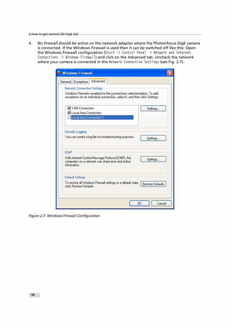
4. No firewall should be active on the network adapter where the Photonfocus GigE camerais connected. If the Windows Firewall is used then it can be switched off like this: Openthe Windows Firewall configuration (Start -> Control Panel -> Network and InternetConnections -> Windows Firewall) and click on the Advanced tab. Uncheck the networkwhere your camera is connected in the Network Connection Settings (see Fig. 2.7).
Figure 2.7: Windows Firewall Configuration
.
16

2.5 Network Adapter Configuration for Pleora eBUS SDK
Open the Network Connections window (Control Panel -> Network and Internet Connections ->Network Connections), right click on the name of the network adapter where the Photonfocuscamera is connected and select Properties from the drop down menu that appears. AProperties window will open. Check the eBUS Universal Pro Driver (see Fig. 2.8) for maximalperformance. Recommended settings for the Network Adapter Card are described in Section2.4.
Figure 2.8: Local Area Connection Properties
2.6 Getting started
This section describes how to acquire images from the camera and how to modify camerasettings.
1. Open the PF_GEVPlayer software (Start -> All Programs -> Photonfocus -> GigE_Tools ->PF_GEVPlayer) which is a GUI to set camera parameters and to see the grabbed images(see Fig. 2.9).
.
2.5 Network Adapter Configuration for Pleora eBUS SDK 17

2 How to get started (3D GigE G2)
Figure 2.9: PF_GEVPlayer start screen
2. Click on the Select / Connect button in the PF_GEVPlayer . A window with all detecteddevices appears (see Fig. 2.10). If your camera is not listed then select the box Showunreachable GigE Vision Devices.
Figure 2.10: GEV Device Selection Procedure displaying the selected camera
3. Select camera model to configure and click on Set IP Address....
.
18

Figure 2.11: GEV Device Selection Procedure displaying GigE Vision Device Information
4. Select a valid IP address for selected camera (see Fig. 2.12). There should be noexclamation mark on the right side of the IP address. Click on Ok in the Set IP Addressdialog. Select the camera in the GEV Device Selection dialog and click on Ok.
Figure 2.12: Setting IP address
5. Finish the configuration process and connect the camera to PF_GEVPlayer .
6. The camera is now connected to the PF_GEVPlayer . Click on the Play button to grabimages.
An additional check box DR1 appears for DR1 cameras. The camera is in dou-ble rate mode if this check box is checked. The demodulation is done in thePF_GEVPlayer software. If the check box is not checked, then the camera out-puts an unmodulated image and the frame rate will be lower than in doublerate mode.
2.6 Getting started 19

2 How to get started (3D GigE G2)
Figure 2.13: PF_GEVPlayer is readily configured
If no images can be grabbed, close the PF_GEVPlayer and adjust the JumboFrame parameter (see Section 2.3) to a lower value and try again.
Figure 2.14: PF_GEVPlayer displaying live image stream
7. Check the status LED on the rear of the camera.
. The status LED light is green when an image is being acquired, and it is red whenserial communication is active.
8. Camera parameters can be modified by clicking on GEV Device control (see Fig. 2.15). Thevisibility option Beginner shows most the basic parameters and hides the more advancedparameters. If you don’t have previous experience with Photonfocus GigE cameras, it isrecommended to use Beginner level.
20

Figure 2.15: Control settings on the camera
9. To modify the exposure time scroll down to the AcquisitionControl control category (boldtitle) and modify the value of the ExposureTime property.
2.6 Getting started 21

2 How to get started (3D GigE G2)
22

3Product Specification
3.1 Introduction
The MV1-D2048x1088-3D03-760-G2-8 is a 2.2 megapixel Gigabit Ethernet CMOS camera fromPhotonfocus optimized for high speed laser triangulation applications with up to 8400profiles/s. The camera includes the detection of up to two laser lines. The laser line detectionalgorithm (Peak Detector) is able to compute the peak position of a laser line with sub-pixelaccuracy. Thus, the height profile of an object gets computed within the camera, makingadditional calculations in the PC needless.
The camera is built around the monochrome CMOS image sensor CMV2000, developed byCMOSIS. The principal advantages are:
• Up to 10200 profiles/s @ 2048 x 23 resolution
• High reliability and accuracy of 3D reconstruction, due to the non-linear interpolationtechnique used in the laser line (peak) detection algorithm
• Laser line (peak) detection with up to 1/64 sub pixel accuracy
• Dual Peak eliminates the need of a second camera for various setups
• 2D single line for 2D surface inspection and image overlay (at full frame rate)
• Gigabit Ethernet interface with GigE Vision and GenICam compliance
• Combined 2D/3D applications can be realized in the 2D/3D mode of the camera (at areduced frame rate)
• Global shutter
• Image sensor with high sensitivity
• Region of interest (ROI) freely selectable in x and y direction
• Column Fixed Pattern Noise Correction for improved image quality.
• Advanced I/O capabilities: 2 isolated trigger inputs, 2 differential isolated RS-422 inputsand 2 isolated outputs
• A/B RS-422 shaft encoder interface
• Programmable Logic Controller (PLC) for powerful operations on input and output signals
• Wide power input range from 12 V (-10 %) to 24 V (+10 %)
• The compact size of only 55 x 55 x 51.5 mm3 makes the MV1-D2048x1088-3D03-760-G2-8camera the perfect solution for applications in which space is at a premium
• Free GUI available (PF 3D Suite) for an easy system set up and visualisation of 3D scans
The basic components for 3D imaging consist of a laser line and a high speed CMOS camera ina triangular arrangement to capture images (profiles) from objects that are moved on aconveyor belt or in a similar setup (see Fig. 3.1 and Section 4.2.2).
You can find more information on the basics of laser triangulation and on theprinciples of 3D image acquisition technique in the user manual "PF 3D Suite"available in the support area at www.photonfocus.com.
23

3 Product Specification
This manual describes version 2.0 of the camera. A list with the functionalitychanges is available in Appendix B.
C o n v e y o r b e l t w i t h o b j e c t s
L a s e r C a m e r a
Figure 3.1: Triangulation principle with objects moved on a conveyor belt
Figure 3.2: Camera MV1-D2048x1088-3D03-760-G2-8
24

3.2 Feature Overview
The general specification and features of the camera are listed in the following sections. Thedetailed description of the camera features is given in Chapter 4.
MV1-D2048x1088-3D03-760-G2
Interface Gigabit Ethernet, GigE Vision, GenICam
Camera Control GigE Vision Suite / PF 3D Suite
Trigger Modes External isolated trigger inputs / Software Trigger / PLC Trigger / AB Trigger
Features Detection of up to 2 laser lines (peak detector)
Linear Mode / multiple slope (High Dynamic Range)
2D single line for 2D surface inspection and image overlay
Grey level resolution 8 bit
Region of Interest (ROI)
Column Fixed Pattern Noise Correction for improved image quality
Isolated inputs (2 single ended, 2 differential) and outputs (2 single ended)
Trigger input / Strobe output with programmable delay
A/B RS-422 shaft encoder interface
Table 3.1: Feature overview (see Chapter 4 for more information)
3.2 Feature Overview 25

3 Product Specification
3.3 Technical Specification
MV1-D2048x1088-3D03-760-G2
Sensor CMOSIS CMV2000
Technology CMOS active pixel
Scanning system progressive scan
Optical format / diagonal 2/3“ (12.76 mm diagonal)
Resolution 2048 x 1088 pixels (2048 x 1024 for one 3D scan area)
Pixel size 5.5 µm x 5.5 µm
Active optical area 11.26 mm x 5.98 mm
Full well capacity ~11 ke−
Spectral range < 350 to 900 nm (to 10 % of peak responsivity)
Conversion gain 0.075 LSB/e−
Sensitivity 5.56 V / lux.s (with micro lenses @ 550 nm)
Optical fill factor 42 % (without micro lenses)
Dark current 125 e−/s @ 25°C
Dynamic range 60 dB
Micro lenses Yes
Colour format monochrome
Characteristic curve Linear, Piecewise linear (multiple slope)
Shutter mode global shutter
Grey scale Resolution 8 bit
Digital Gain 0.1 to 15.99 (Fine Gain)
Exposure Time 12.6 µs ... 0.349 s / 20.8 ns steps
Maximal Frame rate 340 fps (3Donly mode, full resolution)
Table 3.2: General specification of the MV1-D2048x1088-3D03-760-G2
MV1-D2048x1088-3D03-760-G2
Operating temperature 0°C ... 40°C
Camera power supply +12 V DC (- 10 %) ... +24 V DC (+ 10 %)
Trigger signal input range +5 .. +30 V DC
Typical power consumption < 6 W
Lens mount C-Mount
Dimensions 55 x 55 x 51.5 mm3
Mass 260 g
Conformity CE, RoHS, WEEE
Table 3.3: Physical characteristics and operating ranges
26

Fig. 3.3 shows the quantum efficiency curve of the CMV2000 sensor from CMOSIS measured inthe wavelength range from 400 nm to 1000 nm.
0
10
20
30
40
50
60
70
400 500 600 700 800 900 1000
Qu
an
tum
eff
icie
ncy
(%
)
Wavelength (nm)
Spectral response
Figure 3.3: Spectral response of the CMV2000 CMOS image sensor (with micro lenses)
.
3.3 Technical Specification 27

3 Product Specification
28
4Functionality
4.1 Introduction
This chapter serves as an overview of the camera configuration modes and explains camerafeatures. The goal is to describe what can be done with the camera. The setup of theMV1-D2048x1088-3D03-760-G2 camera is explained in later chapters.
4.2 3D Features
4.2.1 Overview
The MV1-D2048x1088-3D03 camera contains a very accurate laser line detector for lasertriangulation (measurement of 3D profiles) that extracts 3D information in real time. For moredetails see Section 4.2.4.
The camera should be placed so that the laser line is located in horizontal direction. Theoutputs of the laser detector (peak detector) are the location coordinate of the laser line, thewidth of the laser line and the grey value of the highest grey value inside the laser line (seeSection 4.2.3).
The camera has a special mode (see 2D&3D mode in Section 4.2.5) for setup and debuggingpurposes that allows to view the image and the detected laser line in the same image.
It is possible to detect one or two laser lines on different parts of the image sensor. This allowsto handle some setups with only one camera where normally two cameras are required (seeTriangulation setups 5 to 7 in Section 4.2.2).
For every laser peak, one complete image row is transmitted in high speed (3Donly) mode. Thisimage row can be used for surface inspection or to produce a 2D overlay image.
4.2.2 Measuring Principle
For a triangulation setup a laser line generator and a camera is used. There are severalconfigurations which are used in the laser triangulation applications. Which setup is used in anapplication is determined by the scattering of the material to be inspected. There are setupsfor highly scattering materials and others for nearly reflecting surfaces.
In addition the penetration depth of light depends on the wavelength of light. The longer thewavelength the deeper is the penetration of the light. Historically red line lasers with awavelength around 630 nm were used. With the modern high power semiconductor line laserin blue (405 nm), green and also in the near infrared there is the possibility to adapt thewavelengths due to the inspection needs.
But not only the penetration depth affects the choice of the wavelength of the line laser. Foran accurate measurement other disturbing effects as radiation or fluorescence of the object orstrong light from neighbourhood processes have to be suppressed by optical filtering and anappropriate selection of the laser wavelength. Hot steel slabs for instance are best inspectedwith blue line laser because of the possibility to separate the laser line with optical filters fromtemperature radiation (Planck radiation) which occurs in red and NIR.
29

4 Functionality
The accuracy of the triangulation system is determinate by the line extracting algorithm, theoptical setup, the quality parameters of the laser line generator and the parameters of the lenswhich makes optical engineering necessary.
Triangulation Setup 1
In this setup the camera looks with the viewing angle α on the laser line projected from thetop. A larger angle leads to a higher resolution. With larger angles the range of height isreduced. Small angles have the benefit of little occlusions.
Camera Line Laser
Figure 4.1: Triangulation setup 1
Triangulation Setup 2
This setup shows an opposite configuration of the laser line and the camera. The resolution atsame triangulation angle is slightly higher but artifacts which occur during the measurement atborders of the object have to be suppressed by software.
Triangulation Setup 3
In this setup the laser line generator and the camera are placed in a more reflectingconfiguration. This gives more signal and could be used for dark or matte surfaces. In case ofreflecting surfaces there is only a little amount of scattering which can be used as signal fortriangulation. Also in this case this triangulation setup helps to get results.
Triangulation Setup 4
In contrast to the setup before this setup is used for high scattering material or for applicationwhere strong reflections of the object have to be suppressed. The resolution is reduced due tothe relations of the angles α and β.
Triangulation Setup 5a
The 3D03 camera has the possibility to detect and determine two laser lines. This gives thepossibility to build up a triangulation setup with two laser lines and one camera to avoid
30

C a m e r aL i n e L a s e r
Figure 4.2: Triangulation setup 2
C a m e r a L i n e L a s e r
Figure 4.3: Triangulation setup 3
occlusions. To reduce the calibration effort a setup with equal angles for the laser lines isbeneficial but not mandatory.
Triangulation Setup 5b
Similar setup to Triangulation Setup 5a, but the angles of the camera and the laser are notequal.
Triangulation Setup 6
The possibility to examine two lines gives the possibility to use the 3D03 camera in setups tomeasure the thickness of glasses or other transparent materials. Additional reflexes whichoccur in such setups could be suppressed by appropriate ROI settings and geometricarrangements.
4.2 3D Features 31

4 Functionality
C a m e r a
L i n e L a s e r
Figure 4.4: Triangulation setup 4
C a m e r aL i n e L a s e r L i n e L a s e r
Figure 4.5: Triangulation setup 5a
Triangulation Setup 7
The two line detection could also be used to eliminate vibrations and elastic deformations ofthe inspected work piece. This is often used in fast profile scanners where the profile guidanceis on the limits. Vibrations and elastic deformations could be detected by interpreting the localheight gradients of the two laser lines during inspection. A change in the 3D profile, forinstance a shape defect, always gives a change in the local gradient, whereas a vibration orelastic deformations does not. This fact can be used in software algorithms to compensatevibration effects and increase the accuracy of the measurements.
4.2.3 Laser Line Detection
The laser line detector takes a threshold value as its input. The threshold has two purposes:
32

C a m e r aL i n e L a s e r L i n e L a s e r
Figure 4.6: Triangulation setup 5b
C a m e r a L i n e L a s e r
G l a s s
Figure 4.7: Triangulation setup 6
• All pixels with grey value below the threshold value will be ignored. This filters out theimage background.
• The value 2*threshold is used in the calculation of the laser line width and height (seebelow).
The output values are calculated column wise (see also Fig. 4.9):
Peak coordinate Vertical coordinate of the laser line peak
Laser line width The laser line width is the number of pixels that have a grey value above2*threshold around the laser peak. If there are no pixels inside the laser line that have agrey level above 2*threshold, then the laser line width is 0. In this case the thresholdvalue should be changed.
Laser line height The laser line height is the highest grey value of the detected laser line. Ifthere are no pixels inside the laser line that have a grey level above 2*threshold, then theheight is set to threshold. In this case the threshold value should be changed.
4.2 3D Features 33

4 Functionality
C a m e r a L i n e L a s e r
Figure 4.8: Triangulation setup 7
The value of the threshold should be set slightly above the grey level of theimage background. However, the value 2*threshold should be smaller than thehighest grey level inside the laser line, otherwise the laser line width and heightare not correctly calculated.
W i d t h
Intensity
y - d i r e c t i o n
G a u s s i a n s h a p e d l a s e r l i n e
T h r e s h o l d
2 * T h r e s h o l d
H e i g h t
P e a k c o o r d i n a t e
Figure 4.9: Schematic of laser line
.
34

4.2.4 Interpolation Technique
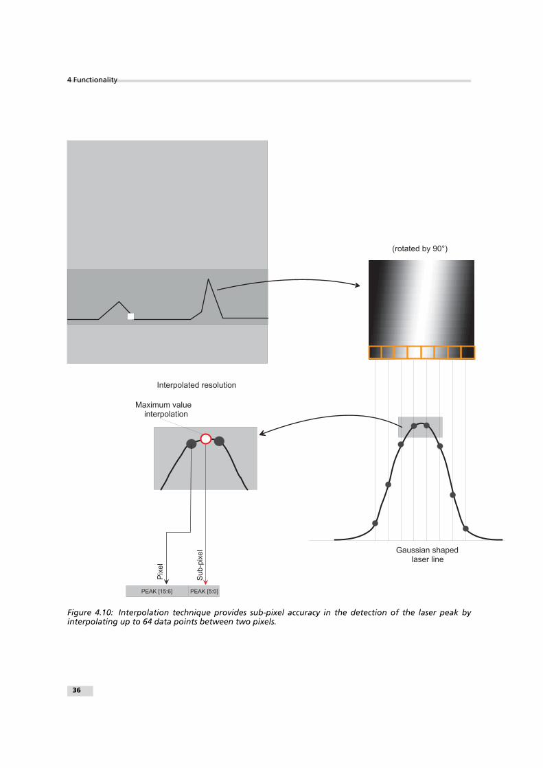
Structured light based systems crucially rely on an accurate determination of the peak positionof the Gaussian shaped laser line. The Peak Detector algorithm in the MV1-D2048x1088-3D03camera applies nonlinear interpolation techniques, where 64 data points are calculatedbetween two pixels within the Gaussian shaped laser line. This technique is superior to othercommonly used detection techniques, such as the detection of peak pixel intensity across thelaser line (resulting in pixel accuracy) or the thresholding of the Gaussian and calculation of theaverage (resulting in sub pixel accuracy).
The nonlinear interpolation technique used in the Peak Detector algorithm results in a betterestimate of the maximum intensity of the laser line. The data mapping for the 3D data block isshown in Section 4.2.9 and the basics of the interpolation principle are illustrated in Fig. 4.10.
The line position (PEAK) is split into a coarse position and a fine position (sub-pixel). The coarseposition is based on the pixel pitch and is transferred in PEAK [15:6]. The sub-pixel positionthat was calculated from the Peak Detector algorithm (6 bit sub-pixel information) is mappedto PEAK [5:0] (see also Section 4.2.9).
Fig. 4.11 shows a comparison of the peak detector algorithm of MV1-D2048x1088-3D03 cameraagainst the Center Of Gravity (COG) algorithm that is used in most triangulation systems. It canclearly be observed that the Peak Detector algorithm gives more accurate results.
.
4.2 3D Features 35
4 Functionality
P E A K [ 1 5 : 6 ] P E A K [ 5 : 0 ]
I n t e r p o l a t e d r e s o l u t i o n
M a x i m u m v a l u e i n t e r p o l a t i o n
Pixel
Sub-pixel
( r o t a t e d b y 9 0 ° )
G a u s s i a n s h a p e d l a s e r l i n e
Figure 4.10: Interpolation technique provides sub-pixel accuracy in the detection of the laser peak byinterpolating up to 64 data points between two pixels.
36
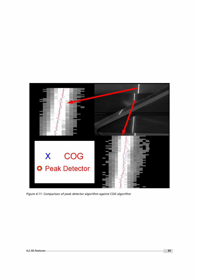
Figure 4.11: Comparison of peak detector algorithm against COG algorithm
4.2 3D Features 37

4 Functionality
4.2.5 3D modes
The camera has three modes that determine which data is transmitted to the user:
2Donly Laser detection is turned off and camera behaves as a normal area scan camera. Thismode serves as a preview mode in the setup and debugging phase.
2D&3D Laser line detection is turned on. The sensor image (2D image) is transmitted togetherwith the 3D data. In the PF 3D Suite, the detected laser line is shown as a coloured line inthe 2D image. This mode serves as a preview mode in the setup and debugging phase ofthe triangulation system.
3Donly Laser line detection is turned on and only 3D data plus an additional image row istransmitted. The scan rate of this mode is considerably faster than the 2D&3D mode.
The 3Donly mode must be used to achieve the highest scan rate.
4.2.6 Peak Mirror
The property Peak[i]_Mirror modifies the output coordinates of peak [i] to Peak[i]_3DH-p[i]-1,where Peak[i]_3DH=height of scan area for peak [i] and p[i] detected laser position for peak [i].PeakMirror can be enabled for each of the 2 peaks individually.
In single peak mode, PeakMirror has roughly the same effect regarding the detected 3Dpositions as rotating the camera by 180°.
In dual peak mode, depending geometrical setup of the camera and the lasers, the orientationof the positions can be different on each peak scan area: e.g. in peak scan area 0, a biggerposition value might indicate a bigger object height, whereas in peak scan area 1, a smallerposition value might indicate a bigger height. The PeakMirror property can be set for one peakto obtain the same orientation for both scan areas.
4.2.7 Single / Dual Peak
It is possible to detect one or two laser lines on different parts of the image sensor (parameterPeakDetector_NrOfPeaks). In dual peak mode (PeakDetector_NrOfPeaks=2) the image sensorcan be divided in two scan areas (see Fig. 4.12). The first laser line (laser line 0) must be locatedin the scan area 0 and the second laser line in the scan area 1. The location and size of the scanareas can be chosen by the user (see also Section 4.3.2).
4.2.8 2D Line
For many tasks it is required or beneficial to have a 2D image of the scanned object. TheMV1-D2048x1088-3D03 camera transmits one image row for every laser peak (see Fig. 4.12). Acomplete 2D image can be obtained by joining the 2D lines. The vertical position of the 2Dlines can be set by the user (property Peak[i]_2DY, replace [i] by 0 or 1).
The illumination outside the laser scan area is normally low. A digital gain (propertyPeak[i]_Gain) and offset (property Peak[i]_DigitalOffset) can be set for the 2D lines to have animage with enough light intensity.
The 2D lines must not be placed inside a laser peak scan area, otherwise the peakdetection will be seriously affected.
38

00
O f f s e t XW
2 0 4 7
1 0 8 7
P e a k 0 _ 2 D Y
P e a k 0 _ 3 D Y
P e a k 0 _ 3 D H
P e a k 1 _ 2 D Y
P e a k 1 _ 3 D Y
P e a k 1 _ 3 D H
S c a n a r e a f o r p e a k 0
S c a n a r e a f o r p e a k 1
2 D l i n e f o r p e a k 1
2 D l i n e f o r p e a k 0
Figure 4.12: ROI definition in 3D modes
4.2.9 3D data format
Cameras with version 2.1 and later have an additional property DataFormat3Dwhich has an effect on the organisation of the 3D data. Camera prior to thisversion have always DataFormat3D=0, although this property is not available.
For every peak there are 4 additional lines that contain the 3D data. Every pixel contains 8 bitsof 3D data which are always placed in the 8 LSB. A table with the bit assignment of the 3D datafor DataFormat3D=0 is shown in Fig. 4.13 and with DataFormat3D=1 in Fig. 4.14. The peak positioncoordinate (PEAK) is relative to the scan area of the peak. To get the absolute position on theimage sensor, the value Peak0_3DY must be added for peak 0 (Peak1_3DY must be added forpeak 1).
LL_HEIGHT and LL_WIDTH values are explained in Fig. 4.13 and in Fig. 4.14.
STAT value: the status (value) of some parameters and internal registers are placed here. Thestatus information is described in Section 4.11.2. In every pixel (column) 4 bits of this statusinformation send, starting with the LSB in the first column.Calculation example (DataFormat3D=0): Suppose that the 3D data of image column n has thefollowing data: 14 / 176 / 10 / 128 (see also Fig. 4.15).
The position of the laser line is in this case 58.75: integer part is calculated from the 8 bits of 3Drow 0 followed by the 2 MSB of 3D row 1: 0b0000111010 = 0x03a = dec 58. The fractional partis calculated from the 6 LSB of 3D row 1: 0b110000 = 0x30. This value must be divided by 64:0x30 / 64 = 0.75.
The laser line width is 10 pixels (6 LSB of 3D row 2).
The LL_HEIGHT value is in this case 8 (=4 MSB of 3D row 3). This means that the 4 MSB of thehighest gray value have the value 8. At 12 bit resolution, the highest gray value lies between0x800 (=2048) and 0x8ff (=2303).
4.2 3D Features 39

4 Functionality
3 D r o w7 6 5 4 3 2 1 0
B i t sD e s c r i p t i o n
0 P E A K [ 1 5 : 8 ] P e a k d e t e c t o r ( l a s e r l i n e ) c o o r d i n a t e
1
2
3
P E A K [ 7 : 0 ]
' 0 ' ' 0 ' L L _ W I D T H [ 5 : 0 ]
P E A K [ 1 5 : 6 ] : i n t e g e r p a r t , P E A K [ 5 : 0 ] : f r a c t i o n a l p a r t
L L _ H E I G H T [ 3 : 0 ] S T A T
L L _ W I D T H : l a s e r l i n e w i d t h
L L _ H E I G H T : h i g h e s t g r e y v a l u e i n s i d e t h e l a s e r l i n e ( 4 M S B ) .S T A T : S t a t u s i n f o r m a t i o n
Figure 4.13: 3D data format, DataFormat3D=0
3 D r o w7 6 5 4 3 2 1 0
B i t sD e s c r i p t i o n
0 P E A K [ 1 5 : 8 ] P e a k d e t e c t o r ( l a s e r l i n e ) c o o r d i n a t e
1
2
3
P E A K [ 7 : 0 ]
L L _ W I D T H [ 3 : 0 ]
P E A K [ 1 5 : 6 ] : i n t e g e r p a r t , P E A K [ 5 : 0 ] : f r a c t i o n a l p a r t
L L _ H E I G H T [ 7 : 0 ]
S T A TL L _ W I D T H : l a s e r l i n e w i d t h ( 4 M S B ) . W i d t h o f l a s e rl i n e i s 4 * L L _ W I D T HS T A T : S t a t u s i n f o r m a t i o n
L L _ H E I G H T : h i g h e s t g r e y v a l u e i n s i d e t h e l a s e r l i n e ( 8 b i t ) .
Figure 4.14: 3D data format. DataFormat3D=1
P o s i t i o n i n t e g r a l p a r t
P o s i t i o n f r a c t i o n a l p a r t
L a s e r l i n e w i d t h
L L _ H E I G H T
3 D r o w7 6 5 4 3 2 1 0
B i t s
0
1
2
3
0 0 0 0 1 1 1 0
1 0 1 1 0 0 0 0
0 0 0 0 1 0 1 0
1 0 0 0 0 0 0 0
Figure 4.15: 3D data calculation example
4.2.10 Transmitted data in 2D&3D mode
The transmitted image in 2D&3D mode is shown in Fig. 4.16. The data is transmitted in thefollowing order:
• Scan area for peak 0
• Scan area for peak 1 (omitted if PeakDetector_NrOfPeaks=1)
• 2D line for peak 0
• 3D data for peak 0
• 2D line for peak 1 (omitted if PeakDetector_NrOfPeaks=1)
• 3D data for peak 1 (omitted if PeakDetector_NrOfPeaks=1)
40

Resulting height in 2D&3D mode is:
Hres = Peak0_3DH + 5 (if PeakDetector_NrOfPeaks=1), or
Hres = Peak0_3DH + Peak1_3DH + 10 (if PeakDetector_NrOfPeaks=2)
0
0W
P e a k 0 _ 3 D H
P e a k 1 _ 3 D H
S c a n a r e a f o r p e a k 0
S c a n a r e a f o r p e a k 1
2 D l i n e f o r p e a k 1
2 D l i n e f o r p e a k 0
3 D d a t a f o r p e a k 0
3 D d a t a f o r p e a k 1
5
5
Figure 4.16: Transmitted image in 2D&3D mode
4.2.11 Transmitted data in 3Donly mode
In 3Donly mode only the 2D lines and the 3D data is transmitted. The FrameCombine feature(see Section 4.2.12) was added to lower the transmitted frame rate. For FrameCombine = f, thedata for f images are combined into one image.
Resulting height in 3Donly mode is therefore:
Hres = f * 5 (if PeakDetector_NrOfPeaks=1), or
Hres = f * 10 (if PeakDetector_NrOfPeaks=2)
W
2 D l i n e f o r p e a k 1 ( i m a g e i )
2 D l i n e f o r p e a k 0 ( i m a g e i )
3 D d a t a f o r p e a k 0 ( i m a g e i )
3 D d a t a f o r p e a k 1 ( i m a g e i )
5
5
2 D l i n e f o r p e a k 1 ( i m a g e i + 1 )
3 D d a t a f o r p e a k 0 ( i m a g e i + 1 )
3 D d a t a f o r p e a k 1 ( i m a g e i + 1 )
5
5
2 D l i n e f o r p e a k 0 ( i m a g e i + 1 )
Figure 4.17: Transmitted image in 3Donly mode with FrameCombine=2
.
4.2 3D Features 41

4 Functionality
4.2.12 Frame Combine
Very high frame rates, that are well over 1000 fps, can be achieved in 3Donly mode. Everyframe (image) activates an interrupt in the GigE software which will issue a high CPU load orthe frame rate can not be handled at all by an overload of interrupts.
To solve this issue, the FrameCombine mode has been implemented in theMV1-D2048x1088-3D03 camera. In this mode, the data of f images are bundled into one frame.In the example shown in Fig. 4.18 4 frames are combined into one frame(FrameCombineNrFrames=4). In this case there are 4 times less software interrupts that indicate anew frame than without FrameCombine and the CPU load is significantly reduced. Instead ofreceiving 4 images with 5 rows, only one image with 20 rows is received which reduces theframe rate that sees the computer. Without FrameCombine, the CPU load on the computermight be too high to receive all images and images might be dropped. The value f(=FrameCombineNrFrames) can be set by the user. This value should be set so that the resultingframe rate is well below 1000 fps (e.g. at 100 fps). E.g. if the camera shows a maximal framerate of 4000 (property AcquisitionFrameRateMax), then FrameCombineNrFrames could be set to 40 tohave a resulting frame rate of 100 fps. Another example of FrameCombineNrFrames=2 isshown in Fig. 4.17. The PF 3D Suite supports this mode.
I n d i v i d u a l i m a g e s
C o m b i n e d i m a g e
F r a m e C o m b i n e
Figure 4.18: Example for FrameCombine with 4 frames
Aborting Frame Combine
There exist possibilities to transmit the combined frame even if there is not enough data to fillit. E.g. It can be desirable to get the 3D data immediately after an item on the conveyor belthas passed.
FrameCombineTimeout A timeout can be specified after which the combined frame will betransmitted, regardless if there was enough data to fill it. The timeout counter is resetafter each frame and counts until a new trigger has been detected or until the timeout isreached.
A FrameCombineTimeout value of 0 disables the FrameCombine timeout fea-ture.
FrameCombineAbort The transmission of the combined frame is forced by writing to theFrameCombineAbort property.
42

When the FrameCombine is aborted, then the remaining data in the combined frame will befilled with filler data: the first two pixels of every filler row have the values 0xBB (decimal 187)and 0x44 (decimal 68). The remaining pixels of the filler rows have the value 0. If looking atthe 3D data, the filler rows seem to have the following values (applying the filler values to the3D data format): the peak positions of the first column is 750.921875, of the second column243.0625 and of the remaining columns 0. The laser line width of the first column is 59, of thesecond column 4 and of the remaining columns 0. LL_HEIGHT is 11 for the first column, 4 forthe second column and 0 for the remaining columns. Status information: the image counter is75 and the remaining status information is 0.
The FrameCombine mode is only available in 3Donly mode.
When acquisition is stopped, then a pending combined frame will be discarded.To get the pending combined frame, a FrameCombineAbort command must besent prior to stopping the acquisition.
4.2 3D Features 43

4 Functionality
4.2.13 Peak Filter
Peaks that are detected by the PeakDetector algorithm can be filtered by applying theparameters described in this section. A filtered peak appears as all 3D data set to 0, which isthe same as if no peak occurred.
Filtering peaks might increase the robustness of the 3D application by filtering peaks that werecaused by unwanted effects, such as reflections of the laser beam. The PeakFilter parameterscan be set for each of the two peaks individually.
PeakFilter parameters (replace [i] by 0 or 1):
Peak[i]_EnPeakFilter Enable peak filtering for peak [i]. If set to False, the PeakFilter settingsare ignored.
Peak[i]_PeakFilterHeightMin Filters all peaks (columns) where 256*LL_HEIGHT <Peak[i]_PeakFilterHeightMin (see Fig. 4.13 and Fig. 4.19).
Peak[i]_PeakFilterHeightMax Filters all peaks (columns) where 256*LL_HEIGHT >Peak[i]_PeakFilterHeightMax (see Fig. 4.13 and Fig. 4.19).
Peak[i]_PeakFilterWidthMin Filters all peaks (columns) where LL_WIDTH <Peak[i]_PeakFilterWidthMin (see Fig. 4.13 and Fig. 4.20).
Peak[i]_PeakFilterWidthMax Filters all peaks (columns) where LL_WIDTH >Peak[i]_PeakFilterWidthMax (see Fig. 4.13 and Fig. 4.20).
An illustration of the PeakFilterHeight parameters is shown in Fig. 4.19. The red line denotes asituation where the laser peak is filtered because the height is too big or too small. Anillustration of the PeakFilterWidth parameters is shown in Fig. 4.20. The red line denotes asituation where the laser peak is filtered because the width is too big or too small.
PeakFilterH
eightM
in
Intensity
y - d i r e c t i o n
T h r e s h o l d
2 * T h r e s h o l d
o k
f i l t e r e d : h e i g h t t o o b i g
f i l t e r e d : h e i g h t t o o s m a l l
PeakFilterH
eightM
ax
Figure 4.19: Illustration of the PeakFilterHeight parameters
.
44

P e a k F i l t e r W i d t h M i n
Intensity
y - d i r e c t i o n
T h r e s h o l d
2 * T h r e s h o l d
P e a k F i l t e r W i d t h M a x
o kf i l t e r e d : w i d t h t o o b i g
f i l t e r e d : w i d t h t o o s m a l l
Figure 4.20: Illustration of the PeakFilterWidth parameters
4.2 3D Features 45

4 Functionality
4.2.14 Absolute Coordinates
The "absolute coordinates" feature is available in camera revision 2.2 and later.
The 3D coordinates are given relative to the start of the 3D ROI as a default.
When the property Peak[i]_EnAbsCoordinate is set to True for peak i then the 3D coordinates aregiven relative to the value of the property Peak[i]_AbsCoordinateBase. This is useful if the3D-ROI is not kept constant.
Example: Peak0_EnAbsCoordinate = True, Peak0_AbsCoordinateBase = 0, Peak0_3DY=200: If the peakis detected in row 50 of the ROI, the value 250 (50+Peak0_3DY) would be given as resulting 3Dcoordinate.
The value of Peak[i]_AbsCoordinateBase must fulfill the following conditions:(Peak[i]_AbsCoordinateBase <= Peak[i]_3DY) and (Peak[i]_AbsCoordinateBase +1024 >= Peak[i]_3DY + Peak[i]_3DH).
MirrorPeak and absolute coordinates
IfPeak[i]_Mirror =True and Peak[i]_EnAbsCoordinate = True then the formula to calculate the 3Dcoordinate is:
c’ = 1024 + Peak[i]_AbsCoordinateBase - Peak[i]_3DY - c - 1,
where c is the original (relative) coordinate without mirroring. This is the same as mirroring ina ROI with Y=Peak[i]_AbsCoordinateBase and H=1024.
4.3 Reduction of Image Size
4.3.1 Region of Interest (ROI) (2Donly mode)
This section describes the ROI features in the 2Donly mode where the camera behaves as astandard area scan camera.
The maximal frame rate of the 2Donly mode is considerably lower than in the3Donly mode.
Some applications do not need full image resolution. By reducing the image size to a certainregion of interest (ROI), the frame rate can be drastically increased. A region of interest can bealmost any rectangular window and is specified by its position within the full frame and itswidth and height. Table 4.1 shows some numerical examples of how the frame rate can beincreased by reducing the ROI.
The ROI is determined by the following properties: OffsetX, Width, OffsetY, Height
Only reductions in height result in a higher frame rate.
46

ROI Dimension MV1-D2048x1088-3D03-760-G2
2048 x 1088 42 fps
1280 x 1024 (SXGA) 45 fps
1280 x 768 (WXGA) 60 fps
800 x 600 (SVGA) 77 fps
640 x 480 (VGA) 96 fps
2048 x 256 179 fps
Table 4.1: Frame rates of different ROI settings in 2Donly mode (exposure time 10 µs; correction on)
4.3.2 Region of Interest (ROI) in 3D modes
The ROI definition in the 3Donly and 2D&3D modes is tailored to laser line detection.
The ROI is determined by the following properties: OffsetX, Width, Peak0_2DY, Peak0_3DY,Peak0_3DH and additionally if PeakDetector_NrOfPeaks=2, Peak1_2DY, Peak1_3DY andPeak1_3DH.
For every peak (laser line) there are two areas (see Fig. 4.12):
One row with 2D data from the image sensor (Peak<n>_2DY) and one area for the detection ofthe laser line <n> (n= 1 or 2) defined by the parameters Peak<n>_3DY, Peak<n>_3DH. Thesevalues can be freely set within the following limits:
1. All regions (2D lines and laser triangulation regions) must not overlap, i.e. no row shouldbe read out more than once.
2. The minimal height of the laser triangulation region (Peak<n>_3DH) is 23 if one peak isused and 29 if two peaks are used.
3. The maximal height of the laser triangulation regions (Peak<n>_3DH) is 1024.
The maximal frame rates for single peak mode are shown in Table 4.2 and in Table 4.3 for dualpeak mode.
Peak0_3DH Width Frame rate 2D&3D mode Frame rate 3Donly mode 1)
23 2048 1440 fps 10126 fps
32 2048 1130 fps 8154 fps
64 2048 635 fps 4793 fps
128 2048 338 fps 2627 fps
256 2048 175 fps 1380 fps
1024 2048 45 fps 358 fps
Table 4.2: Frame rates of different ROI settings in 3D single peak modes (minimal exposure time) (Foot-notes: 1) includes 1 user-selectable image row)
4.3 Reduction of Image Size 47

4 Functionality
Peak0_3DH Peak1_3DH Width Frame rate 2D&3D mode Frame rate 3Donly mode 1)
29 29 2048 634 fps 5123 fps
32 32 2048 586 fps 4732 fps
64 64 2048 324 fps 2608 fps
128 128 2048 171 fps 1374 fps
256 256 2048 88 fps 706 fps
512 512 2048 44 fps 358 fps
1023 1023 2048 22 fps 180 fps
Table 4.3: Frame rates of different ROI settings in 3D dual peak modes (minimal exposure time) (Footnotes:1) includes 1 user-selectable image row for each peak)
48

4.4 Trigger and Strobe
4.4.1 Trigger Source
The trigger signal can be configured to be active high or active low by the TriggerActivation(category AcquisitionControl) property. One of the following trigger sources can be used:
Free running The trigger is generated internally by the camera. Exposure starts immediatelyafter the camera is ready and the maximal possible frame rate is attained, ifAcquisitionFrameRateEnable is disabled. Settings for free running trigger mode:TriggerMode = Off. In Constant Frame Rate mode (AcquisitionFrameRateEnable = True),exposure starts after a user-specified time has elapsed from the previous exposure start sothat the resulting frame rate is equal to the value of AcquisitionFrameRate.
Software Trigger The trigger signal is applied through a software command (TriggerSoftwarein category AcquisitionControl). Settings for Software Trigger mode: TriggerMode = Onand TriggerSource = Software.
Line1 Trigger The trigger signal is applied directly to the camera by the power supplyconnector through pin ISO_IN1 (see also Section A.1). A setup of this mode is shown inFig. 4.21 and Fig. 4.22. The electrical interface of the trigger input and the strobe outputis described in Section 5.5. Settings for Line1 Trigger mode: TriggerMode = On andTriggerSource = Line1.
PLC_Q4 Trigger The trigger signal is applied by the Q4 output of the PLC (see also Section 5.6).Settings for PLC_Q4 Trigger mode: TriggerMode = On and TriggerSource = PLC_Q4.
ABTrigger Trigger from incremental encoder (see Section 4.4.8).
Some trigger signals are inverted. A schematic drawing is shown in Fig. 6.4.
.
4.4 Trigger and Strobe 49

4 Functionality
Figure 4.21: Trigger source
Figure 4.22: Trigger Inputs - Multiple GigE solution
50

4.4.2 Trigger and AcquisitionMode
The relationship between AcquisitionMode and TriggerMode is shown in Table 4.4. WhenTriggerMode=Off, then the frame rate depends on the AcquisitionFrameRateEnable property (seealso under Free running in Section 4.4.1).
The ContinuousRecording and ContinousReadout modes can be used if more thanone camera is connected to the same network and need to shoot images si-multaneously. If all cameras are set to Continuous mode, then all will send thepackets at same time resulting in network congestion. A better way would be toset the cameras in ContinuousRecording mode and save the images in the memoryof the IPEngine. The images can then be claimed with ContinousReadout from onecamera at a time avoid network collisions and congestion.
.
4.4 Trigger and Strobe 51

4 Functionality
AcquisitionMode TriggerMode After the command AcquisitionStart is executed:
Continuous Off Camera is in free-running mode. Acquisition can bestopped by executing AcquisitionStop command.
Continuous On Camera is ready to accept triggers according to theTriggerSource property. Acquisition and triggeracceptance can be stopped by executingAcquisitionStop command.
SingleFrame Off Camera acquires one frame and acquisition stops.
SingleFrame On Camera is ready to accept one trigger according tothe TriggerSource property. Acquisition and triggeracceptance is stopped after one trigger has beenaccepted.
MultiFrame Off Camera acquires n=AcquisitionFrameCount framesand acquisition stops.
MultiFrame On Camera is ready to accept n=AcquisitionFrameCounttriggers according to the TriggerSource property.Acquisition and trigger acceptance is stopped aftern triggers have been accepted.
SingleFrameRecording Off Camera saves one image on the on-board memoryof the IP engine.
SingleFrameRecording On Camera is ready to accept one trigger according tothe TriggerSource property. Trigger acceptance isstopped after one trigger has been accepted andimage is saved on the on-board memory of the IPengine.
SingleFrameReadout don’t care One image is acquired from the IP engine’son-board memory. The image must have beensaved in the SingleFrameRecording mode.
ContinuousRecording Off Camera saves images on the on-board memory ofthe IP engine until the memory is full.
ContinuousRecording On Camera is ready to accept triggers according to theTriggerSource property. Images are saved on theon-board memory of the IP engine until thememory is full. The available memory is 24 MB.
ContinousReadout don’t care All Images that have been previously saved by theContinuousRecording mode are acquired from the IPengine’s on-board memory.
Table 4.4: AcquisitionMode and Trigger
52

4.4.3 Exposure Time Control
The exposure time is defined by the camera. For an active high trigger signal, the camera startsthe exposure with a positive trigger edge and stops it when the programmed exposure timehas elapsed.
External Trigger
In the external trigger mode with camera controlled exposure time the rising edge of thetrigger pulse starts the camera states machine, which controls the sensor and optional anexternal strobe output. Fig. 4.23 shows the detailed timing diagram for the external triggermode with camera controlled exposure time.
e x t e r n a l t r i g g e r p u l s e i n p u t
t r i g g e r a f t e r i s o l a t o r
t r i g g e r p u l s e i n t e r n a l c a m e r a c o n t r o l
d e l a y e d t r i g g e r f o r s h u t t e r c o n t r o l
i n t e r n a l s h u t t e r c o n t r o l
d e l a y e d t r i g g e r f o r s t r o b e c o n t r o l
i n t e r n a l s t r o b e c o n t r o l
e x t e r n a l s t r o b e p u l s e o u t p u t
td - i s o - i n p u t
tj i t t e r
tt r i g g e r - d e l a y
te x p o s u r e
ts t r o b e - d e l a y
td - i s o - o u t p u t
ts t r o b e - d u r a t i o n
tt r i g g e r - o f f s e t
ts t r o b e - o f f s e t
Figure 4.23: Timing diagram for the camera controlled exposure time
The rising edge of the trigger signal is detected in the camera control electronic which isimplemented in an FPGA. Before the trigger signal reaches the FPGA it is isolated from thecamera environment to allow robust integration of the camera into the vision system. In thesignal isolator the trigger signal is delayed by time td−iso−input. This signal is clocked into theFPGA which leads to a jitter of tjitter. The pulse can be delayed by the time ttrigger−delay whichcan be configured by a user defined value via camera software. The trigger offset delayttrigger−offset results then from the synchronous design of the FPGA state machines. Theexposure time texposure is controlled with an internal exposure time controller.
The trigger pulse from the internal camera control starts also the strobe control state machines.The strobe can be delayed by tstrobe−delay with an internal counter which can be controlled bythe customer via software settings. The strobe offset delay tstrobe−delay results then from thesynchronous design of the FPGA state machines. A second counter determines the strobeduration tstrobe−duration(strobe-duration). For a robust system design the strobe output is also
4.4 Trigger and Strobe 53

4 Functionality
isolated from the camera electronic which leads to an additional delay of td−iso−output. Table4.5 gives an overview over the minimum and maximum values of the parameters.
4.4.4 Trigger Delay
The trigger delay is a programmable delay in milliseconds between the incoming trigger edgeand the start of the exposure. This feature may be required to synchronize the external strobewith the exposure of the camera.
4.4.5 Trigger Divider
The Trigger Divider reduces the trigger frequency that is applied to the camera. Every n-thtrigger is processed for a setting of TriggerDivider = n. If n=1, then every trigger is processed(default behaviour). Fig. 6.4 shows the position of the TriggerDivider block.
TriggerDivider is ignored if trigger mode must be set to free-running Trigger(TriggerMode = Off).
4.4.6 Burst Trigger
The camera includes a burst trigger engine. When enabled, it starts a predefined number ofacquisitions after one single trigger pulse. The time between two acquisitions and the numberof acquisitions can be configured by a user defined value via the camera software. The bursttrigger feature works only in the mode "Camera controlled Exposure Time".
The burst trigger signal can be configured to be active high or active low. When the frequencyof the incoming burst triggers is higher than the duration of the programmed burst sequence,then some trigger pulses will be missed. A missed burst trigger counter counts these events.This counter can be read out by the user.
The burst trigger mode is only available when TriggerMode=On. Trigger source is determined bythe TriggerSource property.The timing diagram of the burst trigger mode is shown in Fig. 4.24.
.
54

e x t e r n a l t r i g g e r p u l s e i n p u t
t r i g g e r a f t e r i s o l a t o r
t r i g g e r p u l s e i n t e r n a l c a m e r a c o n t r o l
d e l a y e d t r i g g e r f o r s h u t t e r c o n t r o l
i n t e r n a l s h u t t e r c o n t r o l
d e l a y e d t r i g g e r f o r s t r o b e c o n t r o l
i n t e r n a l s t r o b e c o n t r o l
e x t e r n a l s t r o b e p u l s e o u t p u t
td - i s o - i n p u t
tj i t t e r
tt r i g g e r - d e l a y
te x p o s u r e
ts t r o b e - d e l a y
td - i s o - o u t p u t
ts t r o b e - d u r a t i o n
tt r i g g e r - o f f s e t
ts t r o b e - o f f s e t
d e l a y e d t r i g g e r f o r b u r s t t r i g g e r e n g i n e
tb u r s t - t r i g g e r - d e l a y
tb u r s t - p e r i o d - t i m e
Figure 4.24: Timing diagram for the burst trigger mode
4.4 Trigger and Strobe 55

4 Functionality
MV1-D2048x1088-3D03-760-G2 MV1-D2048x1088-3D03-760-G2
Timing Parameter Minimum Maximum
td−iso−input 1 µs 1.5 µs
td−RS422−input 65 ns 185 ns
tjitter 0 21 ns
ttrigger−delay 0 0.34 s
tburst−trigger−delay 0 0.34 s
tburst−period−time depends on camera settings 0.34 s
ttrigger−offset (non burst mode) 200 ns 167 ns
ttrigger−offset (burst mode) 250 ns 188 ns
texposure 10 µs 0.34 s
tstrobe−delay 600 ns 0.34 s
tstrobe−offset (non burst mode) 200 ns 167 ns
tstrobe−offset (burst mode) 250 ns 188 ns
tstrobe−duration 200 ns 0.34 s
td−iso−output 150 ns 350 ns
ttrigger−pulsewidth 200 ns n/a
Number of bursts n 1 30000
Table 4.5: Summary of timing parameters relevant in the external trigger mode using camera MV1-D2048x1088-3D03-760-G2
56

4.4.7 Software Trigger
The software trigger enables to emulate an external trigger pulse by the camera softwarethrough the serial data interface. It works with both burst mode enabled and disabled. Assoon as it is performed via the camera software, it will start the image acquisition(s),depending on the usage of the burst mode and the burst configuration. The trigger modemust be set to external Trigger (TriggerMode = On).
4.4.8 A/B Trigger for Incremental Encoder
An incremental encoder with differential RS-422 A/B outputs can be used to synchronize thecamera triggers to the speed of a conveyor belt. These A/B outputs can be directly connectedto the camera and appropriate triggers are generated inside the camera.
The A/B Trigger feature is is not available on all camera revisions, see AppendixB for a list of available features.
In this setup, the output A is connected to the camera input ISO_INC0 (see also Section 5.5.4and Section A.1) and the output B to ISO_INC1.
In the camera default settings the PLC is configured to connect the ISO_INC RS-422 inputs tothe A/B camera inputs. This setting is listed in Section 6.11.3.
The following parameters control the A/B Trigger feature:
TriggerSource Set TriggerSource to ABTrigger to enable this feature
ABMode Determines how many triggers should be generated. Available modes: single,double, quad (see description below)
ABTriggerDirection Determines in which direction a trigger should be generated: fwd: onlyforward movement generates a trigger; bkwd: only backward movement generates atrigger; fwdBkwd: forward and backward movement generate a trigger.
ABTriggerDeBounce Suppresses the generation of triggers when the A/B signal bounce.ABTriggerDeBounce is ignored when ABTriggerDirection=fwdbkwd.
ABTriggerDivider Specifies a division factor for the trigger pulses. Value 1 means that allinternal triggers should be applied to the camera, value 2 means that every secondinternal trigger is applied to the camera.
EncoderPosition (read only) Counter (signed integer) that corresponds to the position ofincremental encoder. The counter frequency depends on the ABMode. It counts up/downpulses independent of the ABTriggerDirection. Writing to this property resets the counterto 0.
A/B Mode
The property ABMode takes one of the following three values:
Single A trigger is generated on every A/B sequence (see Fig. 4.25). TriggerFwd is the triggerthat would be applied if ABTriggerDirection=fwd, TriggerBkwd is the trigger that would beapplied if ABTriggerDirection=bkwd, TriggerFwdBkwd is the trigger that would be applied ifABTriggerDirection=fwdBkwd. GrayCounter is the Gray-encoded BA signal that is shown as anaid to show direction of the A/B signals. EncoderCounter is the representation of thecurrent position of the conveyor belt. This value is available as a camera register.
4.4 Trigger and Strobe 57

4 Functionality
Double Two triggers are generated on every A/B sequence (see Fig. 4.26).
Quad Four triggers are generated on every A/B sequence (see Fig. 4.27).
.
A
B
G r a y C o u n t e r
E n c o d e r C o u n t e r
T r i g g e r F w d
T r i g g e r B k w d
0 1 2 3 0 1 2 3 2 1 0 3 2 1 2 3 0
0 1 2 1 0
T r i g g e r F w d B k w d
1
1
Figure 4.25: Single A/B Mode
A
B
G r a y C o u n t e r
E n c o d e r C o u n t e r
T r i g g e r F w d
T r i g g e r B k w d
0 1 2 3 0 1 2 3 2 1 0 3 2 1 2 3 0
0 1 2 3 4 3 2 1 2
T r i g g e r B k w d
1
3
Figure 4.26: Double A/B Mode
A
B
G r a y C o u n t e r
E n c o d e r C o u n t e r
T r i g g e r F w d
T r i g g e r B k w d
0 1 2 3 0 1 2 3 2 1 0 3 2 1 2 3 0
0 1 2 3 4 5 6 7 6 5 4 3 2 1 2 3 4
T r i g g e r F w d B k w d
1
5
Figure 4.27: Quad A/B Mode
.
58

A/B Trigger Debounce
A debouncing logic can be enabled by setting ABTriggerDeBounce=True. It is implemented with awatermark value of the EncoderCounter (see Fig. 4.28). Suppose ABTriggerDirection=fwd, thenthe watermark value is increased with the increments of the EncoderCounter. IfEncoderCounter decreases, e.g. Due to bouncing problems, the watermark value is holdunchanged. Triggers are then only generated when the watermark value increases.
B o u n c i n g
A
B
G r a y C o u n t e r
E n c o d e r C o u n t e r
T r i g g e r F w d
W a t e r m a r k
0 1 3 3 1
0 1 2
22 0
3 3 52 4
0 1 2 543
0 3
4 3
Figure 4.28: A/B Trigger Debouncing, example with ABMode=quad
A/B Trigger Divider
if ABTriggerDivider>1 then not all internally generated triggers are applied to the camera logic.E.g. If ABTriggerDivider=2, then every second trigger is applied to the camera (see Fig. 4.29).
A
B
G r a y C o u n t e r
E n c o d e r C o u n t e r
I n t e r n a l T r i g g e r F w d
0 1 2 3 0 1 2 3 2 1 0 3 2 1 2 3 0
0 1 2 3 4 5 6 7 6 5 4 3 2 1 2 3 4
1
5
A p p l i e d T r i g g e r F w d
Figure 4.29: A/B Trigger Divider, example with ABTriggerDivider=1, ABMode=quad
.
4.4 Trigger and Strobe 59

4 Functionality
A Only Trigger
The camera supports the use of simple incremental decoders that only provide one input, byenabling the property ABTriggerAOnly. The B-signal is ignored in this mode and informationabout direction of the object movement is not available: if ABTriggerAOnly is enabled then theencoder position is always incremented. Detailed diagrams are shown in Fig. 4.30 and Fig.4.31. Note that the quad mode is not available when ABTriggerAOnly=true.
A
E n c o d e r C o u n t e r
T r i g g e r F w d
T r i g g e r B k w d
0 1 2 3 4
T r i g g e r F w d B k w d
5
Figure 4.30: AOnly Trigger in Single A/B Mode
A
E n c o d e r C o u n t e r
T r i g g e r F w d
T r i g g e r B k w d
0 1 2 3 4 5 6 7 9
T r i g g e r F w d B k w d
1 08
Figure 4.31: AOnly Trigger in Double A/B Mode
Encoder Position
The internal ABTrigger signal before the ABTriggerDivider is processed for the EncoderPosition: every TriggerFwd pulse increments the Encoder Position and every TriggerBkwd pulsedecrements its value. For details refer to the diagram of the corresponding mode.
The Encoder Position value can be accessed through the EncoderPosition property or throughthe status info that is inserted into the image (see Section 4.11).
By default the Encoder Position is only generated when TriggerMode=On andTriggerSource=ABTrigger. When the property ABTriggerCountAlways=True, then the EncoderPosition is generated regardless of the trigger mode.
4.4.9 Counter Reset by an External Signal
The image counter and the real time counter (timestamp) (see Section 4.11.1) can be reset byan external signal. Both counters can be embedded into the image by the status line (seeSection 4.11) or their register can be read out. These counters may be used to check that noimages are lost or to ease the synchronisation of multiple cameras.
The external signal to reset the above mentionend counters is selected by the propertyCounter_ResetCounterSource. Available choices are PLC_Q4 to PLC_Q7 (see Section 6.11), Line1(ISO_IN1) and ExposureStart. ExposureStart resets the counters at the start of an exposure.
The property Counter_ResetCounterMode determines how often the selected source should resetthe counters. The setting Once works together with the propertyCounter_ResetCounterOnNextTrigger.
60

If Counter_ResetCounterMode=Once, then the counters are reset on the next active edge of theselected reset source (property Counter_ResetCounterSource) after the device is armed withCounter_ResetCounterOnNextTrigger=True. The register Counter_ResetCounterOnNextTrigger is resetafter the resetting trigger is received.
The setting Counter_ResetCounterMode=Continuous resets the counters on every occurrence of anactive edge of the reset source without the requirement to arm the device first. This setting issuited if the reset source signal is different than the camera trigger.
The active edge of the reset input can be set by the property Counter_ResetCounterSourceInvert.If set to True, then the rising edge is the active edge, else the falling edge.
Counter reset by an external signal is important if you would like to synchronizemultiple cameras. One signal is applied to all cameras which resets the coun-ters simultaneously. The timestamps of all cameras are then theoretically syn-chronous with each other. In practice every camera runs on its own clock sourcewhich has a precision of +/- 30 ppm and therefore the values of the timestamp(real time counter) of the cameras may diverge with time. If this is an issue, thenthe counters could be reset periodically by the external signal.
The counter reset by an external signal feature is not available on all camerarevisions, see Appendix B for a list of available features.
.
4.4 Trigger and Strobe 61

4 Functionality
4.4.10 Trigger Acquisition
The applied trigger can be enabled or disabled by one or two external signals in theTriggerAcquisition mode. This mode works with free-running (internal) trigger and externaltrigger.
The property TriggerAcquisition_Enable enables the TriggerAcquisition mode.
Level Triggered Trigger Acquisition
The Level Triggered mode is enabled by setting TriggerAcquisition_Mode to Level andTriggerAcquisition_Enable=True. A signal acts as a trigger enable (see Fig. 4.32). This signal isselected by TriggerAcquisition_StartSource. A high signal level enables the triggering of thecamera and a low signal level disables all triggers.
To invert the TriggerAcquisition signal use one of the PLC_Q signal and selectthe inverted signal as its source. Table 4.6 shows a setting that uses ISO_IN0 astrigger enable signal: the inverted signal is used as ISO_IN0 is inverted in theinput logic (see Fig. 6.4).
T r i g g e r A c q u i s i t i o n _ S t a r t
T r i g g e r I n
A p p l i e d T r i g g e r
I n t e r n a l T r i g g e r E n a b l e d i s a b l e d e n a b l e d d i s a b l e d
Figure 4.32: Trigger Acquisition Level triggered (TriggerAcquisition_Mode = Level)
Feature Value Category
TriggerAcquisition_Enable True Trigger/TriggerAcquisition
TriggerAcquisition_Mode Level Trigger/TriggerAcquisition
TriggerAcquisition_StartSource PLC_Q5 Trigger/TriggerAcquisition
PLC_I0 Line0 <PLC>/SignalRoutingBlock
PLC_Q5_Variable0 PLC_I0_Not <PLC>/LookupTable/Q5
PLC_Q5_Operator0 Or <PLC>/LookupTable/Q5
PLC_Q5_Variable1 Zero <PLC>/LookupTable/Q5
PLC_Q5_Operator1 Or <PLC>/LookupTable/Q5
PLC_Q5_Variable2 Zero <PLC>/LookupTable/Q5
PLC_Q5_Operator2 Or <PLC>/LookupTable/Q5
PLC_Q5_Variable3 Zero <PLC>/LookupTable/Q5
Table 4.6: Example of using ISO_IN0 as trigger enable in level mode
62

Edge Triggered Trigger Acquisition
The Edge Triggered mode is enabled by setting TriggerAcquisition_Mode to Edge andTriggerAcquisition_Enable=True. Two signals acts as a trigger enable (see Fig. 4.33). A risingedge on the start signal enables triggers. A rising edge on the stop signal disables all triggers.The start/stop signals are selected by TriggerAcquisition_StartSource andTriggerAcquisition_StopSource.
T r i g g e r A c q u i s i t i o n _ S t a r t
T r i g g e r I n
A p p l i e d T r i g g e r
T r i g g e r A c q u i s i t i o n _ S t o p
I n t e r n a l T r i g g e r E n a b l e d i s a b l e d e n a b l e d d i s a b l e d
Figure 4.33: Trigger Acquisition Level triggered (TriggerAcquisition_Mode = Edge)
Trigger Acquisition and Free-Running Trigger
The TriggerAcquisition feature can also be used with free-running trigger (TriggerMode=Off).TriggerAcquisition enables or disables in this case the generation of the free-running trigger.
4.4.11 Strobe Output
he strobe output is an isolated output located on the power supply connector that can be usedto trigger a strobe. The strobe output can be used both in free-running and in trigger mode.There is a programmable delay available to adjust the strobe pulse to your application.
The strobe output needs a separate power supply. Please see Section 5.5, Fig.4.21 and Fig. 4.22 for more information.
4.4 Trigger and Strobe 63

4 Functionality
4.5 High Dynamic Range (multiple slope) Mode
To have an accurate laser line detection it is important that the pixels that represent the laserline, are not saturated. The High Dynamic Range (HDR) mode is a special integration modethat increases the dynamic range of the pixels, and thus avoids the saturation of the pixels inmany cases. The HDR mode is also called multiple slope mode or piecewise linear mode.
The HDR (multi slope) mode clips illuminated pixels which reach a programmable voltage,while leaving the darker pixels untouched (see Fig. 4.34). The clipping level can be adjustedonce (2 slopes) or twice (3 slopes) within the exposure time.
Parameters:
Multislope_Mode There are 3 predefined HDR parameter sets: LowCompression,NormalCompression and HighCompression. If Multislope_Mode is set to UserDefined then theindividual parameters can be set to user defined values.
Multislope_NrSlopes Number of slopes. Multislope_NrSlopes=2: 2 slopes with only knee pointB. Multislope_NrSlopes=3: 3 slopes with knee points A and B.
Multislope_Value1 Corresponds to Vlow1: the higher the value, the higher the compression.
Multislope_Time1 Time corresponding to knee point B. The value is the fraction (per mill) ofthe total exposure time.
Multislope_Value2 Corresponds to Vlow2: the higher the value, the higher the compression.This value is ignored if Multislope_NrSlopes =2.
Multislope_Time2 Time corresponding to knee point A. The value is the fraction (per mill) ofthe total exposure time. This value is ignored if Multislope_NrSlopes =2.
The red line in Fig. 4.34 shows a pixel with high illumination. Without the HDR (3 slopes)mode, the pixel would have reached its saturated value. With HDR mode, the pixel reachesvalue P1 which is below the saturation value. The resulting pixel response in this case is shownin Fig. 4.35. The blue line (P2) shows a pixel with low illumination. Its value never reachesVlow2 or Vlow1 at the knee points and the resulting response is linear.
The parameters Multislope_Value1 and Multislope_Value2 are only applied aftera camera trigger. Note that in free-running mode the camera trigger is appliedinternally by the camera itself.
64

t i m e
V h i g h
V l o w 2 ( M u l t i s l o p e _ V a l u e 2 )
V l o w 1 ( M u l t i s l o p e _ V a l u e 1 )
P 1
P 2
P i x e l r e s e t
K n e e p o i n t A
K n e e p o i n t B
M u l t i s l o p e _ T i m e 2
M u l t i s l o p e _ T i m e 1
E x p o s u r e T i m e
Figure 4.34: Multi Slope (HDR mode)
n u m b e r o f e l e c t r o n s
S a t u r a t i o n l e v e l
O u t p u t s i g n a l
K n e e p o i n t A
K n e e p o i n t B
Figure 4.35: Piecewise linear response
4.5 High Dynamic Range (multiple slope) Mode 65

4 Functionality
4.6 Data Path Overview
The data path is the path of the image from the output of the image sensor to the output ofthe camera. The sequence of blocks is shown in figure Fig. 4.36.
I m a g e S e n s o r
D i g i t a l O f f s e t
D i g i t a l G a i n
P e a k D e t e c t o r
I m a g e o u t p u t
T e s t i m a g e s i n s e r t i o n
( r a m p / L F S R )
L a s e r t e s t i m a g e
i n s e r t i o n
O u t l i e r s C o r r e c t i o n
C o l u m n F P N
C o r r e c t i o n
Figure 4.36: camera data path
.
66

4.7 Column FPN Correction
The camera contains a correction to decrease the Column Fixed Pattern Noise (FPN) of thesensor. By default the Column FPN Correction is enabled.
The Column FPN Correction of the camera is correctly calibrated at the Photonfocus productionfacility. Although a new calibration is normally not required, the user can recalibrate theColumn FPN Correction. No light should be applied to the camera during calibration. Theaverage grey value of every column of the image is calculated. The difference to the averagegrey value of the whole image is then calculated for every column and stored in internalcamera memory. After calibration, this difference is then subtracted column-wise from everyimage to reduce the Column FPN. Detailed instructions on the calibration of the Column FPNCorrection is given in Section 6.7.
4.8 Outliers Correction
Defective pixels of the image sensor might appear as dark or bright pixels. Although this is notcommon, a defective pixel correction (Outliers Correction) is implemented in the camera. Bydefault the outliers corrections for black pixels and for white pixels are enabled.
A pixel is labeled as a black pixel if the grey value is smaller than the parameter BlackLimit andthe grey value differences to its two neighbours on the same row exceed the value of theparameter BlackDiff (see Fig. 4.37). The Black Pixel Outliers correction can be enabled ordisabled by a property (see also Section 6.8). If it is enabled then a black outlier pixel isreplaced by the mean of the grey values of its two neighbours on the same row.
Similarly a pixel is labeled as a white pixel if the grey value is bigger than the parameterWhiteLimit and the grey value differences to its two neighbours on the same row exceed thevalue of the parameter WhiteDiff (see Fig. 4.37). The White Pixel Outliers correction can beenabled or disabled by a property (see also sec_gui_outliers_corr). If it is enabled then a whiteoutlier pixel is replaced by the mean of the grey values of its two neighbours on the same row.
B l a c k P i x e l C o r r e c t i o n
R a w i m a g e
I n t e n s i t y
B l a c k L i m i tD i f f L e f t D i f f R i g h t
D i f f L e f t > B l a c k D i f f A N D D i f f R i g h t > B l a c k D i f f
C o r r e c t e d i m a g e
W h i t e P i x e l C o r r e c t i o n
W h i t e L i m i t
D i f f L e f t D i f f R i g h t
D i f f L e f t > W h i t e D i f f A N D D i f f R i g h t > W h i t e D i f f
Figure 4.37: Outliers correction
.
4.7 Column FPN Correction 67
4 Functionality
4.9 Gain and Offset
There are three different gain settings on the camera:
Analog Gain Analog gain on the image sensor (only available in some models, see AppendixB). Available values: x1, x1.2, x1.4, x1.6. Note that Digital Offset is applied after theAnalog Gain.
Gain (Digital Fine Gain) Digital fine gain accepts fractional values from 0.01 up to 15.99. It isimplemented as a multiplication operation. Colour camera models only: There isadditionally a gain for every RGB colour channel. The RGB channel gain is used tocalibrate the white balance in an image, which has to be set according to the currentlighting condition.
Digital Gain Digital Gain is a coarse gain with the settings x1, x2, x4 and x8. It is implementedas a binary shift of the image data where ’0’ is shifted to the LSB’s of the gray values. E.g.for gain x2, the output value is shifted by 1 and bit 0 is set to ’0’.
The resulting gain is the product of the three gain values, which means that the image data ismultiplied in the camera by this factor.
Digital Fine Gain and Digital Gain may result in missing codes in the output im-age data.
A user-defined value can be subtracted from the gray value in the digital offset block. If digitalgain is applied and if the brightness of the image is too big then the interesting part of theoutput image might be saturated. By subtracting an offset from the input of the gain block itis possible to avoid the saturation.
4.10 Laser test image
A Laser Test Image has been added that resembles a moving laser line (see Fig. 4.38) and it isplaced just before the peak detection. Therefore it can be used to test if the 3D data iscorrectly processed during application development.
4.11 Image Information and Status Information
There are camera properties available that give information about the acquired images, suchas an image counter and the number of missed trigger signals. These properties can be queriedby software.
4.11.1 Counters
Image counter The image counter provides a sequential number of every image that is output.After camera startup, the counter counts up from 0 (counter width 24 bit). The countercan be reset by the camera control software.
Real Time counter (Time stamp) The time counter starts at 0 after camera start, and countsreal-time in units of 1 micro-second. The time counter can be reset by the software in theSDK (Counter width 32 bit).
Missed trigger counter The missed trigger counter counts trigger pulses that were ignored bythe camera because they occurred within the exposure or read-out time of an image. Infree-running mode it counts all incoming external triggers (counter width 8 bit / no wraparound).
68

Figure 4.38: Laser test image
Missed burst trigger counter The missed burst trigger counter counts trigger pulses that wereignored by the camera in the burst trigger mode because they occurred while the camerastill was processing the current burst trigger sequence.
Missed FrameCombine trigger counter Counts missed triggers due to the FrameCombinefeature (see also Section 4.2.12). A missed FrameCombine trigger can occur if a trigger isapplied while filler rows are added to a frame due to a FrameCombine abort.
4.11.2 Status Information
Status information is inserted in the 4 LSB in the last 3D data row (see bits labeled STAT in Fig.4.13). LSB are transmitted first (see Table 4.7). The status information is divided in fields of 32bits each, where every information field corresponds to one information parameter (see Table4.8). Unused bits are set to 0.
Col 0 Col 1 Col 2 Col 3 ... Col n
STAT[3:0] STAT[7:4] STAT[11:8] STAT[15:12] ... STAT[4*n+3:4*n]
Table 4.7: STAT value
4.12 Test Images
Test images are generated in the camera FPGA, independent of the image sensor. They can beused to check the transmission path from the camera to the acquisition software. Independentfrom the configured grey level resolution, every possible grey level appears the same numberof times in a test image. Therefore, the histogram of the received image must be flat.
A test image is a useful tool to find data transmission errors or errors in the accessof the image buffers by the acquisition software.
4.12 Test Images 69

4 Functionality
Status bits Parameter Description
STAT[23:0] IMG_CNT[23:0] Image counter (see also Section 4.11.1)
STAT[63:32] RT_CNT[31:0] Real time counter (time stamp) (see also Section4.11.1)
STAT[87:64] ENC_POS[23:0] Encoder position (see also Section 4.4.8)
STAT[103:96] M_TRIG[7:0] Missed trigger counter (see also Section 4.11.1)
STAT[135:128] M_BURST_TRIG[7:0] Missed burst trigger counter (see also Section 4.11.1)
STAT[167:160] M_FC_TRIG[7:0] Missed FrameCombine trigger counter (see alsoSection 4.11.1)
Table 4.8: Status fields
The analysis of the test images with a histogram tool gives a flat histogram onlyif the image width is a multiple of 256 (in 8 bit mode).
.
70

4.12.1 Ramp
Depending on the configured grey level resolution, the ramp test image outputs a constantpattern with increasing grey level from the left to the right side (see Fig. 4.39).
Figure 4.39: Ramp test images: 8 bit output
4.12.2 LFSR
The LFSR (linear feedback shift register) test image outputs a constant pattern with apseudo-random grey level sequence containing every possible grey level that is repeated forevery row. The LFSR test pattern was chosen because it leads to a very high data toggling rate,which stresses the interface electronic and the cable connection.
Figure 4.40: LFSR (linear feedback shift register) test image
In the histogram you can see that the number of pixels of all grey values are the same.
Please refer to application note [AN026] for the calculation and the values of the LFSR testimage.
4.12 Test Images 71

4 Functionality
4.12.3 Troubleshooting using the LFSR
To control the quality of your complete imaging system enable the LFSR mode, set the camerawindow to 1024 x 1024 pixels (x=0 and y=0) and check the histogram. If your image acquisitionapplication does not provide a real-time histogram, store the image and use a graphic softwaretool (e.g. ImageJ) to display the histogram.
In the LFSR (linear feedback shift register) mode the camera generates a constantpseudo-random test pattern containing all grey levels. If the data transmission is correctlyreceived, the histogram of the image will be flat (Fig. 4.41). On the other hand, a non-flathistogram (Fig. 4.42) indicates problems, that may be caused either by a defective camera, byproblems in the acquisition software or in the transmission path.
Figure 4.41: LFSR test pattern received and typical histogram for error-free data transmission
Figure 4.42: LFSR test pattern received and histogram containing transmission errors
In robots applications, the stress that is applied to the camera cable is especially high due tothe fast movement of the robot arm. For such applications, special drag chain capable cablesare available. Please contact the Photonfocus Support for consulting expertise.
72

5Hardware Interface
5.1 GigE Connector
The GigE cameras are interfaced to external components via
• an Ethernet jack (RJ45) to transmit configuration, image data and trigger.
• a 12 pin subminiature connector for the power supply, Hirose HR10A-10P-12S (female) .
The connectors are located on the back of the camera. Fig. 5.1 shows the plugs and the statusLED which indicates camera operation.
E t h e r n e t J a c k ( R J 4 5 )
P o w e r S u p p l ya n d I / O C o n n e c t o r
S t a t u s L E D
Figure 5.1: Rear view of the GigE camera
5.2 Power Supply Connector
The camera requires a single voltage input (see Table 3.3). The camera meets all performancespecifications using standard switching power supplies, although well-regulated linear powersupplies provide optimum performance.
It is extremely important that you apply the appropriate voltages to your camera.Incorrect voltages will damage the camera.
73

5 Hardware Interface
A suitable power supply can be ordered from your Photonfocus dealership.
For further details including the pinout please refer to Appendix A.
5.3 Status Indicator (GigE cameras)
A dual-color LED on the back of the camera gives information about the current status of theGigE CMOS cameras.
LED Green It blinks slowly when the camera is not grabbing images.When the camera isgrabbing images the LED blinks at a rate equal to the frame rate. At slowframe rates, the LED blinks. At high frame rates the LED changes to anapparently continuous green light, with intensity proportional to the ratio ofreadout time over frame time.
LED Red Red indicates an active serial communication with the camera.
Table 5.1: Meaning of the LED of the GigE CMOS cameras
5.4 Power and Ground Connection for GigE G2 Cameras
The interface electronics is isolated from the camera electronics and the power supplyincluding the line filters and camera case. Fig. 5.2 shows a schematic of the power and groundconnections.
.
74
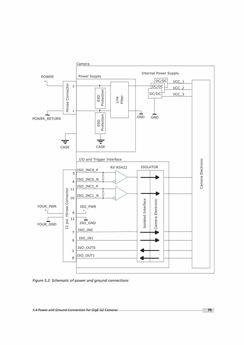
P o w e r S u p p l y
2
P O W E R _ R E T U R N
1
C A S E
G N D
I n t e r n a l P o w e r S u p p l y
D C / D C V C C _ 3
+
P O W E R
R X R S 4 2 2I S O _ I N C 0 _ P
I S O _ I N C 0 _ N
I S O _ I N C 1 _ P
I S O _ I N C 1 _ N
I S O _ I N 0
I S O _ I N 1
I S O _ O U T 0
I S O _ O U T 1
Isolated Interface
Camera Electronic
I S O L A T O R
I S O _ G N D
I S O _ P W R
1 2
12 pol. H
irose C
onnector
6
8
3
9
7
1 0
1 1
4
5
+
I / O a n d T r i g g e r I n t e r f a c e
D C / D C
D C / D C
V C C _ 2
V C C _ 1
ESD
Protection
ESD
Protection
Camera Electronic
Line
Filter
Y O U R _ G N D
Y O U R _ P W R
+
Hirose C
onnector
C A S E
G N D
C a m e r a
Figure 5.2: Schematic of power and ground connections
5.4 Power and Ground Connection for GigE G2 Cameras 75

5 Hardware Interface
5.5 Trigger and Strobe Signals for GigE G2 Cameras
5.5.1 Overview
The 12-pol. Hirose power connector contains two external trigger inputs, two strobe outputsand two differential RS-422 inputs. All inputs and outputs are connected to the ProgrammableLogic Controller (PLC) (see also Section 5.6) that offers powerful operations.
The pinout of the power connector is described in Section A.1.
ISO_INC0 and ISO_INC1 RS-422 inputs have -10 V to +13 V extended commonmode range.
ISO_OUT0 and ISO_OUT1 have different output circuits (see also Section 5.5.2).
A suitable trigger breakout cable for the Hirose 12 pol. connector can be orderedfrom your Photonfocus dealership.
Simulation with LTSpice is possible, a simulation model can be downloaded fromour web site www.photonfocus.com on the software download page (in Supportsection). It is filed under "Third Party Tools".
Fig. 5.3 shows the schematic of the inputs and outputs. All inputs and outputs are isolated.ISO_VCC is an isolated, internally generated voltage.
.
76

I S O _ G N D
R X R S 4 2 2I S O _ I N C 0 _ P
I S O _ I N C 0 _ N
M A X 3 0 9 8
I S O _ I N C 1 _ P
I S O _ I N C 1 _ N
I S O _ G N D
I S O _ V C C
e n h a n c e d
P o w e r F E T4 . 7 V
1 0 kI S O _ I N 0
G N D I S O _ G N D
I S O _ V C C
e n h a n c e d
P o w e r F E T4 . 7 V
1 0 kI S O _ I N 1
I S O _ G N D
I S O _ P W R
P o w e r
M O S F E T
I S O _ O U T 0P T C 4 k 7
M a x . 3 0 V
M a x . 0 . 5 A
M a x . 0 . 5 W
I S O _ G N D
P o w e r
M O S F E T
I S O _ O U T 1P T C
M a x . 3 0 V
M a x . 0 . 5 A
M a x . 0 . 5 W
Isolated Interface
Camera Electronic
- 1 0 V t o + 1 3 V e x t e n d e d
C o m m o n M o d e R a n g e
I S O L A T O R
I S O _ G N D
I S O _ P W R
1 2
12 pol. H
irose C
onnector
6
8
3
9
7
1 0
1 1
4
5
+
+
+
+
C a m e r a
M i n . - 3 0 V
M a x . 3 0 V
M i n . - 3 0 V
M a x . 3 0 V
I S O _ V C C
+
Figure 5.3: Schematic of inputs and output
5.5 Trigger and Strobe Signals for GigE G2 Cameras 77

5 Hardware Interface
5.5.2 Single-ended Inputs
ISO_IN0 and ISO_IN1 are single-ended isolated inputs. The input circuit of both inputs isidentical (see Fig. 5.3).
Fig. 5.4 shows a direct connection to the ISO_IN inputs.
In the camera default settings the PLC is configured to connect the ISO_IN0 tothe PLC_Q4 camera trigger input. This setting is listed in Section 6.11.2.
I S O _ G N D I S O _ G N D
I S O _ V C C
e n h a n c e d
P o w e r F E T4 . 7 V
1 0 kI S O _ I N 0
C a m e r a
7
1 2 p o l . H i r o s e
C o n n e c t o r
I S O _ G N D
1 2
Y O U R _ G N D Y O U R _ G N D
I n p u t V o l t a g e
M a x . + 3 0 V D C
M i n . - 3 0 V D C
+
Figure 5.4: Direct connection to ISO_IN
Fig. 5.5 shows how to connect ISO_IN to TTL logic output device.
I S O _ G N D I S O _ G N D
I S O _ V C C
e n h a n c e d
P o w e r F E T4 . 7 V
1 0 kI S O _ I N 0
C a m e r a
7
1 2 p o l . H i r o s e
C o n n e c t o r
I S O _ G N D
1 2
Y O U R _ G N D Y O U R _ G N D
C o n t r o l L o g i c
&
Y O U R _ V C C +
+
Figure 5.5: Connection to ISO_IN from a TTL logic device
.
78

5.5.3 Single-ended Outputs
ISO_OUT0 and ISO_OUT1 are single-ended isolated outputs.
ISO_OUT0 and ISO_OUT1 have different output circuits: ISO_OUT1 doesn’t havea pullup resistor and can be used as additional Strobe out (by adding Pull up) oras controllable switch. Maximal ratings that must not be exceeded: voltage: 30V, current: 0.5 A, power: 0.5 W.
Fig. 5.6 shows the connection from the ISO_OUT0 output to a TTL logic device. PTC is a currentlimiting device.
I S O _ G N D
I S O _ P W R
P o w e r
M O S F E T
I S O _ O U T 0P T C4 k 7
C a m e r a
3
1 2 p o l . H i r o s e
C o n n e c t o r
I S O _ G N D
1 2
Y O U R _ G N D
I S O _ P W R Y O U R _ P W R
Y O U R _ G N D
C o n t r o l L o g i c
&
Y O U R _ P W R
+ + + +6
M a x . 3 0 V
M a x . 0 . 5 A
M a x . 0 . 5 W
Figure 5.6: Connection example to ISO_OUT0
Fig. 5.7 shows the connection from ISO_OUT1 to a TTL logic device. PTC is a current limitingdevice.
I S O _ G N D
P o w e r
M O S F E T
I S O _ O U T 1P T C
C a m e r a
8
1 2 p o l . H i r o s e
C o n n e c t o r
I S O _ G N D
1 2
Y O U R _ G N D Y O U R _ G N D
C o n t r o l L o g i c
&
Y O U R _ P W R
+
4 k 7
+
Y O U R _ P W R
M a x . 3 0 V
M a x . 0 . 5 A
M a x . 0 . 5 W
Figure 5.7: Connection from the ISO_OUT1 output to a TTL logic device
.
5.5 Trigger and Strobe Signals for GigE G2 Cameras 79

5 Hardware Interface
Fig. 5.8 shows the connection from ISO_OUT1 to a LED.
Y O U R _ P W R
I S O _ G N D
P o w e r
M O S F E T
I S O _ O U T 1P T C R
C a m e r a
8
1 2 p o l . H i r o s e
C o n n e c t o r
I S O _ G N D
1 2
Y O U R _ G N D
+
Figure 5.8: Connection from ISO_OUT1 to a LED
Respect the limits of the POWER MOSFET in the connection to ISEO_OUT1. Max-imal ratings that must not be exceeded: voltage: 30 V, current: 0.5 A, power: 0.5W. (see also Fig. 5.9). The type of the Power MOSFET is: International RectifierIRLML0100TRPbF.
Y O U R _ P W R
I S O _ G N D
P o w e r
M O S F E T
I S O _ O U T 1P T C
L
C a m e r a
8
1 2 p o l . H i r o s e
C o n n e c t o r
I S O _ G N D
1 2
Y O U R _ G N D
Y O U R _ P W R
LDD
D
1
2
M a x . 3 0 V
M a x . 0 . 5 A
M a x . 0 . 5 W
+ +
R e s p e c t t h e l i m i t s o f t h e P O W E R M O S F E T !
Figure 5.9: Limits of ISO_OUT1 output
.
80

5.5.4 Differential RS-422 Inputs
ISO_INC0 and ISO_INC1 are isolated differential RS-422 inputs (see also Fig. 5.3). They areconnected to a Maxim MAX3098 RS-422 receiver device. Please consult the data sheet of theMAX3098 for connection details.
Don’t connect single-ended signals to the differential inputs ISO_INC0 andISO_INC1 (see also Fig. 5.10).
R X R S 4 2 2
I S O _ I N C x _ P
I S O _ I N C x _ N
1 2 p o l . H i r o s e
C o n n e c t o r
Y O U R _ G N D
5 V T T L L o g i c L e v e l
C a m e r a
Figure 5.10: Incorrect connection to ISO_INC inputs
5.5.5 Master / Slave Camera Connection
The trigger input of one Photonfocus G2 camera can easily connected to the strobe output ofanother Photonfocus G2 camera as shown in Fig. 5.11. This results in a master/slave modewhere the slave camera operates synchronously to the master camera.
I S O _ G N D
I S O _ P W R
P o w e r
M O S F E T
I S O _ O U T 0P T C4 k 7
I S O _ G N D I S O _ G N D
I S O _ V C C
e n h a n c e d
P o w e r F E T4 . 7 V
1 0 kI S O _ I N 0
M a s t e r C a m e r a S l a v e C a m e r a
3
7
H i r o s e
C o n n e c t o r s
+ +
I S O _ G N D I S O _ G N D
1 2 1 2
6
I S O _ P W R
Figure 5.11: Master / slave connection of two Photonfocus G2 cameras
.
5.5 Trigger and Strobe Signals for GigE G2 Cameras 81

5 Hardware Interface
5.6 PLC connections
The PLC (Programmable Logic Controller) is a powerful device where some camera inputs andoutputs can be manipulated and software interrupts can be generated. Sample settings and anintroduction to PLC are shown in Section 6.11. PLC is described in detail in the document [PLC].
Name Direction Description
A0 (Line0) Power connector -> PLC ISO_IN0 input signal
A1(Line1) Power connector -> PLC ISO_IN1 input signal
A2 (Line2) Power connector -> PLC ISO_INC0 input signal
A3 (Line3) Power connector -> PLC ISO_INC1 input signal
A4 camera head -> PLC FVAL (Frame Valid) signal
A5 camera head -> PLC LVAL (Line Valid) signal
A6 camera head -> PLC DVAL (Data Valid) signal
A7 camera head -> PLC Reserved (CL_SPARE)
Q0 PLC -> not connected
Q1 PLC -> power connector ISO_OUT1 output signal (signal is inverted)
Q2 PLC -> not connected
Q3 PLC -> not connected
Q4 PLC -> camera head PLC_Q4 camera trigger
Q5 PLC -> camera head Reserved for future use
Q6 PLC -> camera head Incremental encoder A signal
Q7 PLC -> camera head Incremental encoder B signal
Table 5.2: Connections to/from PLC
82

6Software
6.1 Software for MV1-D2048x1088-3D03-G2
Various software packages for Photonfocus MV1-D2048x1088-3D03-G2 camera are available onthe Photonfocus website:
eBUS SDK Contains the Pleora SDK and the Pleora GigE filter drivers. Many examples of theSDK are included.
PFInstaller Contains the PF_GEVPlayer, the PF 3D Suite and SDK, a property list for every GigEcamera and additional documentation and examples.
PF 3D Suite and SDK Visualization tool for Photonfocus 3D cameras. This tool is described in aseparate manual [MAN053] and is included in the PFInstaller.
6.2 PF_GEVPlayer
The camera parameters can be configured by a Graphical User Interface (GUI) tool for GigabitEthernet Vision cameras or they can be programmed with custom software using the SDK.
A GUI tool that can be downloaded from Photonfocus is the PF_GEVPlayer. How to obtain andinstall the software and how to connect the camera is described in Chapter 2.
After connecting to the camera, the camera properties can be accessed by clicking on the GEVDevice control button (see also Section 6.2.2).
The PF_GEVPlayer is described in more detail in the GEVPlayer Quick Start Guide[GEVQS] which is included in the PFInstaller.
There is also a GEVPlayer in the Pleora eBUS package. It is recommended touse the PF_GEVPlayer as it contains some enhancements for Photonfocus GigEcameras such as decoding the image stream in DR1 cameras.
83

6 Software
6.2.1 PF_GEVPlayer main window
After connecting the camera (see Chapter 2), the main window displays the following controls(see Fig. 6.1):
Disconnect Disconnect the camera
Mode Acquisition mode
Play Start acquisition
Stop Stop acquisition
Acquisition Control Mode Continuous, Single Frame or Multi Frame modes. The number offrames that are acquired in Multi Frame mode can be set in the GEV Device Control withAcquisitionFrameCount in the AcquisitionControl category.
Communication control Set communication properties.
GEV Device control Set properties of the camera head, IP properties and properties of the PLC(Programmable Logic Controller, see also Section 5.6 and document [PLC]).
Image stream control Set image stream properties and display image stream statistics.
Figure 6.1: PF_GEVPlayer main window
Below the image display there are two lines with status information
6.2.2 GEV Control Windows
This section describes the basic use of the GEV Control windows, e.g. the GEV Device Controlwindow.
The view of the properties in the control window can be changed as described below. At startthe properties are grouped in categories which are expanded and whose title is displayed inbold letters. An overview of the available view controls of the GEV Control windows is shownin Fig. 6.2.
84

To have a quick overview of the available categories, all categories should be collapsed. Thecategories of interest can then be expanded again. If the name of the property is known, thenthe alphabetical view is convenient. If this is the first time that you use a Photonfocus GigEcamera, then the visibility should be left to Beginner.
The description of the currently selected property is shown at the bottom ot the window.
After selecting a property from a drop-down box it is necessary to press <Enter>or to click with the mouse on the control window to apply the property value tothe camera.
A red cross at the upper right corner of the GEV Control Window indicates aparameter error, i.e. a parameter is not correctly set. In this case you shouldcheck all properties. A red exclamation mark (!) at the right side of a parametervalue indicates that this parameters has to be set correctly.
T o g g l e c a t e g o r y /a l p h a b e t i c a l v i e w
E x p a n d a l lc a t e g o r i e s
C o l l a p s e a l lc a t e g o r i e s
V i s i b i l i t ys e l e c t i o n
E x p a n dc a t e g o r y
C o l l a p s ec a t e g o r y
P r o p e r t yd e s c r i p t i o n
P a r a m e t e re r r o r
i n d i c a t i o n
Figure 6.2: PF_GEVPlayer Control Window
.
6.2 PF_GEVPlayer 85

6 Software
6.2.3 Display Area
The images are displayed in the main window in the display area. A zoom menu is availablewhen right clicking in the display area. Another way to zoom is to press the Ctrl button whileusing the mouse wheel.
6.2.4 White Balance (Colour cameras only)
A white balance utility is available in the PF_GEVPlayer in Tools -> Image Filtering (see Fig.6.3). The gain of the colour channels can be adjusted manually by sliders or an auto whitebalance of the current image can be set by clicking on the White Balance button. To have acorrect white balance setting, the camera should be pointed to a neutral reference (object thatreflects all colours equally), e.g. a special grey reference card while clicking on the WhiteBalance button.
The white balance settings that were made as described in this section, are ap-plied by the PF_GEVPlayer software and are not stored in the camera. To storethe colour gain values in the camera, the Gain settings in the GEV Device Control(in AnalogControl) must be used. If the gain properties in the camera are used,then the PF_GEVPlayer RGB Filtering should be disabled.
Figure 6.3: PF_GEVPlayer image filtering dialog
6.2.5 Save camera setting to a file
The current camera settings can be saved to a file with the PF_GEVPlayer (File -> Save or SaveAs...). This file can later be applied to camera to restore the saved settings (File -> Open), Note,that the Device Control window must not be open to do this.
The MROI and LUT settings are not saved in the file.
86

6.2.6 Get feature list of camera
A list of all features of the Photonfocus G2 cameras in HTML format can be found in theGenICam_Feature_Lists sub-directory (in Start -> All Programs -> Photonfocus -> GigE_Tools).
Alternatively, the feature list of the connected camera can be retrieved with the PF_GEVPlayer(Tools -> Save Camera Features as HTML...).
6.3 Pleora SDK
The eBUS package provides the PureGEV C++ SDK for image acquisition and the setting ofproperties. A help file is installed in the Pleora installation directory, e.g. C:\ProgramFiles\Pleora Technologies Inc\eBUS SDK\Documentation.
Various code samples are installed in the installation directory, e.g. C:\Program Files\PleoraTechnologies Inc\eBUS SDK\Samples. The sample PvPipelineSample is recommended to start with.
Samples that show how to set device properties are included in the PFInstaller that can bedownloaded from the Photonfocus webpage.
6.4 Frequently used properties
The following list shows some frequently used properties that are available in the Beginnermode. The category name is given in parenthesis.
Width (ImageFormatControl) Width of the camera image ROI (region of interest)
Height (ImageFormatControl) Width of the camera image ROI
OffsetX, OffsetY (ImageFormatControl) Start of the camera image ROI
ExposureTime (AcquisitionControl) Exposure time in microseconds
TriggerMode (AcquisitionControl) External triggered mode
TriggerSource (AcquisitionControl) Trigger source if external triggered mode is selected
Header_Serial (Info / CameraInfo) Serial number of the camera
UserSetSave (UserSetControl) Saves the current camera settings to non-volatile flash memory.
6.5 Height setting
The Height property must be set manually to the value of HeightInterface whenever a propertyrelevant to the height setting is modified (an example for this can be found in Section 6.6). Theheight relevant properties are:
• PeakDetector_NrOfPeaks
• PeakDetector_Mode
• Peak0_3DH
• Peak1_3DH
• FrameCombine
The height can be directly written to the Height property in 2Donly mode.
6.3 Pleora SDK 87

6 Software
6.6 3D (Peak Detector) settings
This section describes how to the set the 3D properties. These properties are described inSection 4.2.
1. Set threshold value for peak 0 with property Peak0_Threshold (in categoryPeakDetector/Peak0) (see also note in Section 4.2.3).
2. Set scan area for peak 0 by setting the start row (Peak0_3DY in category PeakDetector/Peak0)the height (Peak0_3DH in category PeakDetector/Peak0) (see also Section 4.3.2).
3. Set image (2D) row for peak 0 by setting Peak0_2DY (in category PeakDetector/Peak0). Notethat this value must be outside the scan areas.
4. If two peaks are required then repeat steps 1 to 3 with peak 1, replacing Peak0 with Peak1in the property names.
5. Set PeakDetector_Mode (in category PeakDetector) to Mode_3Donly or to Mode_2Dand3D. Notethat Mode_3Donly should be selected for maximal frame rate.
6. Set PeakDetector_NrOfPeaks to the required number of peaks (1 or 2).
7. If PeakDetector_Mode is set to Mode_2Dand3D then skip steps 8 to 10 and continue at step 11.
8. The number of frames of the FrameCombine feature (FrameCombine_NrOfFrames) should beset to a value that the resulting frame rate is below 200 for most applications (see alsoSection 4.2.12). The resulting frame rate is the trigger rate divided byFrameCombine_NrOfFrames. In free running mode (TriggerMode = Off) the frame rate can beread from the property AcquisitionFrameRateMax (in category AcquisitionControl). Thelower the resulting frame rate, the fewer interrupts are generated by the GigE driver andthe less load is produced on the computer’s CPU. E.g. if the trigger rate is 4000 fps thenFrameCombine_NrOfFrames should be set to 20 or more.
9. If FrameCombine is used, then the parameter FrameCombine_Timeout (in microseconds)should be set (see also Section 4.2.12. The value should be higher than the longest timebetween triggers, e.g. if the trigger rate is constant, then it could be set to twice the timebetween triggers.
10. If FrameCombine is used then FrameCombine_Enable should be set to True.
11. Read the value of the parameter HeightInterface and set Height to this value.
6.7 Column FPN Correction
6.7.1 Enable / Disable the Column FPN Correction
The Column FPN Correction can be enabled or disabled with the property ColCorrection_Enable(in category Correction/ColCorrection). By default the correction is enabled.
6.7.2 Calibration of the Column FPN Correction
The Column FPN Correction of the camera is correctly calibrated at Photonfocus productionfacility. Although a new calibration is normally not required, you can recalibrate the ColumnFPN Correction with the following instructions:
1. Setup the camera to the mode where it will be usually used. (Exposure time, ...). Thewidth should be set to its maximal value. Due to the internal structure of the camera, bestperformance of calibration will be achieved when calibrating under "real conditions".When the camera will be run in 3Donly mode, which is required for maximal frame rate,then the following settings should be applied: PeakDetector_Mode = Mode_3Donly (category
88

PeakDetector), PeakDetector_NrOfPeaks = 1 (category PeakDetector), Peak0_3DY = 0 (categoryPeakDetector / Peak0 / Peak0_3D,) Peak0_3DH = 1024 (category PeakDetector / Peak0 / Peak0_3D,Peak0_2DY = 1024 (category PeakDetector / Peak0 / Peak0_2D), Width = 2048 (categoryImageFormatControl), Height = 5 (category ImageFormatControl)
. If different exposure times will be used, calibrate the camera under the longestexposure time.
2. Put the camera in free-running mode by setting the property TriggerMode to Off.
3. Start grabbing of the camera by clicking on the Play button.
4. Wait until the camera has achieved working temperature.
5. Close the lens of the camera or put a cap on the lense.
6. Set the visibility of the Device Control window of the PF_GEVPlayer to Expert.
7. Run the command ColCorrection_CalibrateBlack (category Correction / ColCorrection) byclicking on the corresponding button. The camera transmits a test image duringcalibration.
8. Run the command ColCorrection_Update by clicking on the corresponding button. Read theColCorrection_Busy value which should be 0 after the calibration has finished. Repeat thisstep if its value is not 0. If the ColCorrection_Busy value doesn’t show 0 after various tries,check if the camera receive triggers or set the TriggerMode of the camera to Off.
9. Check the values of the properties ColCorrection_Overflow and ColCorrection_Underflow. Bothshould have the value 0 after calibration. If ColCorrection_Overflow is not 0, then decreaseBlackLevel (in category AnalogControl) and re-run the procedure from step 6 on. IfColCorrection_Underflow is not 0, then increase BlackLevel (in category AnalogControl) andre-run the procedure from step 6 on.
10. The Column FPN correction is now calibrated. The calibration values are stored in thecamera’s RAM and these values are lost when the camera power is turned off. To store thecalibration values to permanent memory see Section 6.7.3.
6.7.3 Storing the calibration in permanent memory
After running the calibration procedure (see Section 6.7.2) the calibration values are stored inRAM. When the camera is turned off, their values are lost.
To prevent this, the calibration values must be stored in flash memory. This can be done byclicking on the property ColCorrection_SaveToFlash (in category Calibration). Wait until thecommand has been finished, i.e.the property ColCorrection_Busy (category Correction /ColCorrection) is 0. ColCorrection_Busy can be updated by clicking on the propertyColCorrection_Update (in category Calibration).
6.8 Outliers Correction
The Outliers Correction feature is explained in Section 4.8. This section shows its properties.
6.8.1 Black Pixel Correction
The Black Pixel Outliers Correction can be enabled by the propertyOutliersCorrection_EnBlackPixel (in category Correction / OutliersCorrection / BlackPixel). Ablack pixel must have a grey value smaller than OutliersCorrection_BlackLimit and the minimaldifference to its two neighbours on the same row is OutliersCorrection_BlackDiff. All valuesare specified at 12 bit resolution, i.e. 4095 is the value for a saturated pixel.
6.8 Outliers Correction 89

6 Software
6.8.2 White Pixel Correction
The White Pixel Outliers Correction can be enabled by the propertyOutliersCorrection_EnWhitePixel (in category Correction / OutliersCorrection / WhitePixel). AWhite pixel must have a grey value bigger than OutliersCorrection_WhiteLimit and the minimaldifference to its two neighbours on the same row is OutliersCorrection_WhiteDiff. All valuesare specified at 12 bit resolution, i.e. 4095 is the value for a saturated pixel.
6.9 Permanent Parameter Storage / Factory Reset
The property UserSetSave (in category UserSetControl) stores the current camera settings in thenon-volatile flash memory. At power-up these values are loaded.
The property UserSetSave (in category UserSetControl) overwrites the current camera settingswith the settings that are stored in the flash memory.
The command CameraHeadFactoryReset (in category PhotonfocusMain) restores the settings of thecamera head
The property CameraHeadStoreDefaults (in category PhotonfocusMain) stores onlythe settings of the camera head in the flash memory. It is recommended to useUserSetSave instead, as all properties are stored.
The calibration values of the FPN calibration are not stored with UserSetSave (orCameraHeadStoreDefaults). Use the command Correction_SaveToFlash for this (seeCorrection_SaveToFlash).
6.10 Persistent IP address
It is possible to set a persistent IP address:
1. Set GevPersistentIPAddress (in category TransportLayerControl) to the desired IP address.
2. Set GevPersistentSubnetMask (in category TransportLayerControl) to the sub net mask.
3. Set GevCurrentIPConfigurationPersistent (in category TransportLayerControl) to True.
4. Set GevCurrentIPConfigurationDHCP (in category TransportLayerControl) to False.
5. The selected persistent IP address will be applied after a reboot of the camera.
.
90

6.11 PLC Settings
6.11.1 Introduction
The Programmable Logic Controller (PLC) is a powerful tool to generate triggers and softwareinterrupts. A functional diagram of the PLC tool is shown in Fig. 6.4. The PLC tool is describedin detail with many examples in the [PLC] manual which is included in the PFInstaller.
The AB Trigger feature is not available on all camera revisions, see Appendix Bfor a list of available features.
A 0 ( L i n e 0 )A 1 ( L i n e 1 )
S i g n a lR o u t i n gB l o c k
A 4A 5A 6A 7
P L C7I S O _ I N 09I S O _ I N 1
I S O _ I N C 0 _ P5
4I S O _ I N C 0 _ NI S O _ I N C 1 _ P 1 1
1 0I S O _ I N C 1 _ N
P o w e r C o n n e c t o r
I / O d e c o u p l i n g
F V A LL V A LD V A L
R E S E R V E D
P L C _ c t r l 0P L C _ c t r l 1P L C _ c t r l 2P L C _ c t r l 3
Q 2Q 3Q 6Q 7
p g 0 _ o u tp g 1 _ o u tp g 2 _ o u tp g 3 _ o u t
d e l _ o u t
r s l _ o u tg p _ c n t _ e qg p _ c n t _ g t
t s _ t r i g 0t s _ t r i g 1t s _ t r i g 2t s _ t r i g 3
L o o k u pT a b l e
I 1
I 2
I 3
I 4
I 5
I 6
I 7
I 0
E n h a n c e dF u n c t i o nB l o c k
Q 0Q 1Q 2Q 3
Q 4Q 5Q 6Q 7
Q 8Q 9
Q 1 0Q 1 1
Q 1 5Q 1 6Q 1 7
R e m o t eC o n t r o lB l o c kfr
om
host PC
8I S O _ O U T 1
I m a g eC o n t r o lB l o c k
Q 1 2Q 1 3Q 1 4
T r i g g e r S o f t w a r e
T r i g g e r S o u r c e
F r e e - r u n n i n g t r i g g e rI n t e r n a l c a m e r a t r i g g e r
T r i g g e r M o d e
3I S O _ O U T 0S t r o b e
A 2 ( L i n e 2 )A 3 ( L i n e 3 )
L i n e 1
P L C _ Q 4
S o f t w a r eO f f
O n1C A M E R A _ G N D2C A M E R A _ P W R6I S O _ P W R1 2I S O _ G N D
I / O d e c o u p l i n g , i n v e r t i n g
T r i g g e rD i v i d e r
A BT r i g g e r
A
B
A B T r i g g e r D i v i d e rA B T r i g g e r M o d e
A B T r i g g e r D i r e c t i o nA B T r i g g e r D e b o u n c eA B T r i g g e r A O n l y
A B T r i g g e r
T r i g g e r S o u r c e
Figure 6.4: PLC functional overview and trigger connections
The simpliest application of the PLC is to connect a PLC input to a PLC output. The connectionof the ISO_IN0 input to the PLC_Q4 camera trigger is given as an example. The resultingconfiguration is shown in Section 6.11.2.
6.11 PLC Settings 91

6 Software
1. Identify the PLC notation of the desired input. A table of the PLC mapping is given inSection 5.6. In our example, ISO_IN0 maps to A0 or Line0.
2. Select a Signal Routing Block (SRB) that has a connection to the desired PLC input andconnect it to the PLC input. In our example, SRB PLC_I0 will be used as it has a connectionto Line0. To connect the SRB to input, set PLC_I<x> to the input. In the example, set PLC_I0to Line0.
3. Identify the PLC notation of the desired output. A table of the PLC mapping is given inSection 5.6. In the example Q4 is the desired output.
4. Connect the LUT that corresponds to the desired output to the SRB from step 2. In theexample, PLC_Q4 is connected to PLC_I0. Note that every LUT has the capability to connectup to 4 inputs. In the example only the first input (PLC_Q4_Variable0) is used. The otherinputs are ignored by setting the PLC_Q4_Variable to Zero and the PLC_Q4_Operator toOr for inputs 1 to 3.
5. If a PLC output is used to connect to a camera trigger, then the corresponding TriggerSource must be activated. In the example, TriggerSource is set to PLC_Q4 and TriggerModeis set to On.
6.11.2 PLC Settings for ISO_IN0 to PLC_Q4 Camera Trigger
This setting connects the ISO_IN0 to the internal camera trigger, see Section 6.11.2 (the visibilityin the PF_GEVPlayer must be set to Guru for this purpose).
Feature Value Category
TriggerMode On AcquisitionControl
TriggerSource PLC_Q4 AcquisitionControl
PLC_I0 Line0 <PLC>/SignalRoutingBlock
PLC_Q4_Variable0 PLC_I0_Not <PLC>/LookupTable/Q4
PLC_Q4_Operator0 Or <PLC>/LookupTable/Q4
PLC_Q4_Variable1 Zero <PLC>/LookupTable/Q4
PLC_Q4_Operator1 Or <PLC>/LookupTable/Q4
PLC_Q4_Variable2 Zero <PLC>/LookupTable/Q4
PLC_Q4_Operator2 Or <PLC>/LookupTable/Q4
PLC_Q4_Variable3 Zero <PLC>/LookupTable/Q4
Table 6.1: PLC Settings for ISO_IN0 to PLC_Q4 Camera Trigger (<PLC> = in categoryIPEngine/ProgrammableLogicController)
.
92

6.11.3 PLC Settings for A/B Trigger from differential inputs
This settings connects the ISO_INC RS-422 inputs to the A/B camera inputs. ISO_INC0 is mappedto the A signal and ISO_INC1 to the B signal, see Table 6.2 (the visibility in the PF_GEVPlayermust be set to Guru for this purpose).
The AB Trigger feature is not available on all camera revisions, see Appendix Bfor a list of available features.
Feature Value Category
TriggerMode On AcquisitionControl
TriggerSource ABTrigger AcquisitionControl
PLC_I2 Line2 <PLC>/SignalRoutingBlock
PLC_I3 Line3 <PLC>/SignalRoutingBlock
PLC_Q6_Variable0 PLC_I2 <PLC>/LookupTable/Q6
PLC_Q6_Operator0 Or <PLC>/LookupTable/Q6
PLC_Q6_Variable1 Zero <PLC>/LookupTable/Q6
PLC_Q6_Operator1 Or <PLC>/LookupTable/Q6
PLC_Q6_Variable2 Zero <PLC>/LookupTable/Q6
PLC_Q6_Operator2 Or <PLC>/LookupTable/Q6
PLC_Q6_Variable3 Zero <PLC>/LookupTable/Q6
PLC_Q7_Variable0 PLC_I3 <PLC>/LookupTable/Q7
PLC_Q7_Operator0 Or <PLC>/LookupTable/Q7
PLC_Q7_Variable1 Zero <PLC>/LookupTable/Q7
PLC_Q7_Operator1 Or <PLC>/LookupTable/Q7
PLC_Q7_Variable2 Zero <PLC>/LookupTable/Q7
PLC_Q7_Operator2 Or <PLC>/LookupTable/Q7
PLC_Q7_Variable3 Zero <PLC>/LookupTable/Q7
Table 6.2: PLC Settings for A/B Trigger from differential inputs (<PLC> = in categoryIPEngine/ProgrammableLogicController)
.
6.11 PLC Settings 93

6 Software
6.11.4 PLC Settings for A/B Trigger from single-ended inputs
This configuration maps the single-ended inputs to the A/B camera inputs: ISO_IN0 is mappedto the A signal and ISO_IN1 to the B signal see Table 6.3 (the visibility in the PF_GEVPlayer mustbe set to Guru for this purpose).
The AB Trigger feature is not available on all camera revisions, see Appendix Bfor a list of available features.
Feature Value Category
TriggerMode On AcquisitionControl
TriggerSource ABTrigger AcquisitionControl
PLC_I0 Line0 <PLC>/SignalRoutingBlock
PLC_I1 Line1 <PLC>/SignalRoutingBlock
PLC_Q6_Variable0 PLC_I0 <PLC>/LookupTable/Q6
PLC_Q6_Operator0 Or <PLC>/LookupTable/Q6
PLC_Q6_Variable1 Zero <PLC>/LookupTable/Q6
PLC_Q6_Operator1 Or <PLC>/LookupTable/Q6
PLC_Q6_Variable2 Zero <PLC>/LookupTable/Q6
PLC_Q6_Operator2 Or <PLC>/LookupTable/Q6
PLC_Q6_Variable3 Zero <PLC>/LookupTable/Q6
PLC_Q7_Variable0 PLC_I1 <PLC>/LookupTable/Q7
PLC_Q7_Operator0 Or <PLC>/LookupTable/Q7
PLC_Q7_Variable1 Zero <PLC>/LookupTable/Q7
PLC_Q7_Operator1 Or <PLC>/LookupTable/Q7
PLC_Q7_Variable2 Zero <PLC>/LookupTable/Q7
PLC_Q7_Operator2 Or <PLC>/LookupTable/Q7
PLC_Q7_Variable3 Zero <PLC>/LookupTable/Q7
Table 6.3: PLC Settings for A/B Trigger from single-ended inputs (<PLC> = in categoryIPEngine/ProgrammableLogicController)
94

7Mechanical and Optical Considerations
7.1 Mechanical Interface
During storage and transport, the camera should be protected against vibration, shock,moisture and dust. The original packaging protects the camera adequately from vibration andshock during storage and transport. Please either retain this packaging for possible later use ordispose of it according to local regulations.
7.1.1 Cameras with GigE Interface
Fig. 7.1 shows the mechanical drawing of the camera housing for the Photonfocus 2048 GigEcamera series.
55
55
20
12.8
25.4
36.6
41.3
5 51.5
8x M5
60.8
Figure 7.1: Mechanical dimensions of the Photonfocus 2048 GigE cameras
For long life and high accuracy operation, we highly recommend to mount thecamera thermally coupled, so that the mounting acts as a heat sink. To verifyproper mounting, camera temperature can be monitored using the GeniCamcommand DeviceTemperature under GEVDeviceControl.
95

7 Mechanical and Optical Considerations
7.2 CE compliance
The Photonfocus camera MV1-D2048x1088-3D03-760-G2-8 is in compliance with the belowmentioned standards according to the provisions of European Standards Directives:
• EN 61 000 - 6 - 3 : 2001
• EN 61 000 - 6 - 2 : 2001
• EN 61 000 - 4 - 6 : 1996
• EN 61 000 - 4 - 4 : 1996
• EN 61 000 - 4 - 3 : 1996
• EN 61 000 - 4 - 2 : 1995
• EN 55 022 : 1994
96

8Warranty
The manufacturer alone reserves the right to recognize warranty claims.
8.1 Warranty Terms
The manufacturer warrants to distributor and end customer that for a period of two yearsfrom the date of the shipment from manufacturer or distributor to end customer (the"Warranty Period") that:
• the product will substantially conform to the specifications set forth in the applicabledocumentation published by the manufacturer and accompanying said product, and
• the product shall be free from defects in materials and workmanship under normal use.
The distributor shall not make or pass on to any party any warranty or representation onbehalf of the manufacturer other than or inconsistent with the above limited warranty set.
8.2 Warranty Claim
The above warranty does not apply to any product that has been modified or al-tered by any party other than manufacturer, or for any defects caused by any useof the product in a manner for which it was not designed, or by the negligenceof any party other than manufacturer.
97

8 Warranty
98

9References
All referenced documents can be downloaded from our website at www.photonfocus.com.
AN007 Application Note "Camera Acquisition Modes", Photonfocus, March 2004
GEVQS GEVPlayer Quick Start Guide, Pleora Technologies. Included in eBUS installer.
MAN051 Manual "Photonfocus GigE Quick Start Guide", Photonfocus
MAN053 Manual "PF 3D Suite", Photonfocus
PLC iPORT Programmable Logic Controller Reference Guide, Pleora Technologies. Included inGigE software package.
99

9 References
100

APinouts
A.1 Power Supply Connector
The power supply connectors are available from Hirose connectors atwww.hirose-connectors.com. Fig. A.1 shows the power supply plug from the solder side. Thepin assignment of the power supply plug is given in Table A.2.
It is extremely important that you apply the appropriate voltages to your camera.Incorrect voltages will damage or destroy the camera.
The connection of the input and output signals is described in Section 5.5.
A suitable power supply can be ordered from your Photonfocus dealership.
Connector Type Order Nr.
12-pole Hirose HR10A-10P-12S soldering 110-0402-0
12-pole Hirose HR10A-10P-12SC crimping 110-0604-4
Table A.1: Power supply connectors (Hirose HR10 series, female connector)
91
1 21 1
1 0 8
7
65
4
3
2
Figure A.1: Power supply connector, 12-pole female (rear view of connector, solder side)
101

A Pinouts
Pin I/O Type Name Description
1 PWR CAMERA_GND Camera GND, 0V
2 PWR CAMERA_PWR Camera Power 12V..24V
3 O ISO_OUT0 Default Strobe out, internally Pulled up to ISO_PWRwith 4k7 Resistor
4 I ISO_INC0_N INC0 differential RS-422 input, negative polarity
5 I ISO_INC0_P INC0 differential RS-422 input, positive polarity
6 PWR ISO_PWR Power supply 5V..24V for output signals; Do NOTconnect to camera Power
7 I ISO_IN0 IN0 input signal
8 O ISO_OUT1 (MISC) Q1 output from PLC, no Pull up to ISO_PWR ; can beused as additional output (by adding Pull up) or ascontrollable switch (max. 100mA, no capacitive orinductive load)
9 I ISO_IN1(Trigger IN) Default Trigger IN
10 I ISO_INC1_N INC1 differential RS-422 input, negative polarity
11 I ISO_INC1_P INC1 differential RS-422 input, positive polarity
12 PWR ISO_GND I/O GND, 0V
Table A.2: Power supply connector pin assignment
102

BCamera Change Log
This chapter lists changes of the camera functionality from one camera version to another.
Always the newest camera revision is shipped if not otherwise mentioned by the customer. If aprevious version is required then this must be clearly mentionend on the purchase order. See inthe specific revision section for more information.
The version of your camera is stored in the property uCRevision (in category Info / CameraInfo,set visibility to Expert). It is a number with at least 5 digits. The two rightmost digits are thebuild number, the next two digits (counting from the right side) are the minor revision numberand the remaining digits are the major revision number. uCRevision=10203 would thereforeindicate the version 1.2 (build 3).
B.1 Revision 1.1 / 04.04.2012
First version. uCRevision = 10100.
Not recommended for new designs.
Order information: Order number 605030.101, MV1-D2048x1088-3D03-760-G2-8 R1
B.2 Revision 2.0 / 04.01.2013
uCRevision = 20000.
• 3D frame rate increased.
• Maximal 3D scan area increased to 2048x1024 pixels.
• Added gain and digital offset function to the 2D line.
• PeakFilter can be set individually for each peak.
• Added MirrorPeak function.
• A/B Trigger: added ABTriggerAOnly.
• Encoder position indication: optionally the encoder position is calculated also whentrigger source is not ABTrigger (property ABTriggerCountAlways).
• Column Fixed Pattern Noise (FPN) Correction added.
• Outliers Correction (black and white pixel) added.
• Test images added.
• Green status LED now blinks also when camera is not grabbing images to always see ifcamera is powered.
• Improvement: in FrameCombine mode, image counter is now incremented with everyimage from sensor. Previously the image counter was incremented for every combinedimage, resulting in the same image number for all frames in one combined frame.
• Bug fixed: the applied FrameCombineTimeout value is now as set by the property. Previouslyit was ten times smaller than set.
• Bug fixed: in the previous version, the status info bits disappeared when UserSetSavecommand was issued. This is now solved.
103

B Camera Change Log
• Improvement: the values of the status info bits are captured at exposure start. Previouslyit was sampled at the time when the status info bits are inserted into the image.
B.3 Revision 2.1 / 14.02.2013
uCRevision = 20100.
• New property DataFormat3D introduced which enables the output of 8 bit intensity values(LL_HEIGHT) instead of 4 bit values (DataFormat3D=1). In this mode the laser line width(LL_WIDTH) is reduced to 4 bits instead of 6 bits. The position of these parameters in the 3Ddata is also modified if DataFormat3D=1. DataFormat3D=0 is the default mode which is thesame as in previous revisions.
B.4 Revision 2.2 / 18.11.2013
uCRevision = 20200.
• New feature absolute coordinates added (see Section 4.2.14).
B.5 Revision 2.3 / 14.02.2014
uCRevision = 20300.
• New feature Counter Reset by an External Signal added (see Section 4.4.9).
• New feature Trigger Acquisition added (see Section 4.4.10).
104

CRevision History
Revision Date Changes
1.0 February 2012 First version
1.1 February 2012 Chapter "Product Specification": camera dimensions and lensmount corrected.
Chapter "Mechanical Interface": mechanical drawing corrected.Note about thermal coupling of the camera added.
1.2 February 2012 Chapter "Functionality", section "3D Features" / "Peak Filter":Diagrams added; Property PeakFilter_EnPeakNr removed.
Chapter "Functionality", section "Reduction of Image Size":frame rates corrected
Chapter "Functionality", section "Exposure Time Control":trigger-controlled exposure time removed
Chapter "Functionality", section "A/B Trigger for IncrementalEncoder": ABTriggerResolution renamed to ABTriggerDivider(ABTriggerDivder = ABTriggerResolution+1)
Chapter "Functionality". section "High Dynamic Range(multiple slope) Mode" added.
1.3 April 2012 Chapter "Product Specification": full well capacity corrected to11 ke− (from 13.5 ke−).
1.4 May 2012 Adapted to PFInstaller_2_30 and later
105

C Revision History
Revision Date Changes
2.0 January 2013 Chapter Product Specification, section Technical Specification:minimal exposure time corrected. Value of 1µs was notcorrect. Maximal 3D scan area increased to 2048x1024 pixels.
Chapter Functionality, section 3D Features: 2D line is nowdescribed in its own section. Added section Mirror Peak.
Chapter Functionality, section 3D Features (3D data format):added STAT description and reference to status informationsection.
Chapter Functionality, section 3D Features (Peak Filter):parameters can now be set for every peak.
Chapter Functionality, section 3D Features (Frame Combine /Aborting Frame Combine): More text about value of the fillerrows added.
Chapter Functionality, section Reduction of Image Size (Regionof Interest (ROI) in 3D modes): frame rates are higher incamera version 2.
Chapter Functionality, section Trigger and Strobe: sectionsTrigger Divider, A Only Trigger and Encoder Position (both inA/B Trigger for Incremental Encoder) added.
Chapter Functionality: sections Column FPN Correction, OutliersCorrection and Test Images added.
Chapter Hardware Interface, section Status Indicator (GigEcameras): green LED now blinks also when camera is idle.
Chapter Software, sections Column FPN Correction and OutliersCorrection.
Chapter Software, section PLC Settings: PLC drawing improved.
2.1 February 2013 Chapter Functionality, section 3D data format (3D Features):new property DataFormat3D introduced.
Chapter Functionality, section Region of Interest (ROI) in 3Dmodes (Reduction of Image Size): description improved.
2.2 November 2013 FrameCombine documentation improved.New feature"absolute coordinates" added.
2.3 February 2014 Section Peak Filter: property names corrected.
Section Reduction of Image Size: frame rates corrected
Section Counter Reset by an External Signal added.
Section Trigger Acquisition added.
Camera Revision 2.3 added.
106


