Manager Sentiment and Stock Returns

Fuwei Jiang

Central University of Finance and Economics

Joshua Lee

Florida State University-Tallahassee

Xiumin Martin

Washington University in St. Louis

Guofu Zhou∗

Washington University in St. Louis

First Version: April 2015

Current Version: October 2015

∗Corresponding author. Send correspondence to Guofu Zhou, Olin School of Business, Washington University inSt. Louis, St. Louis, MO 63130; e-mail: zhou@wustl.edu; phone: 314-935-6384. We are grateful to John Doukas,Xingguo Luo, Jianfeng Yu, and seminar participants at Washington University in St. Louis, Zhejiang University,Central University of Finance and Economics for very helpful comments.

Manager Sentiment and Stock Returns

Abstract

In this paper, we construct a manager sentiment index based on the aggregated textual

tone of conference calls and financial statements. We find that manager sentiment is

a strong negative predictor of future aggregate stock market returns, with monthly in-

sample and out-of-sample R2 of 9.75% and 8.38%, respectively, which is far greater

than the predictive power of other previously-studied macroeconomic variables. Its

predictive power is also stronger than and is complimentary to the popular investor

sentiment indexes. Moreover, manager sentiment also negatively predicts future

aggregate earnings and cross-sectional stock returns, particularly for those firms that

are either hard to value or difficult to arbitrage.

JEL classifications: C53, G11, G12, G17

Keywords: Manager Sentiment, Textual Tone, Asset Pricing, Return Predictability

1

1. Introduction

Many studies in behavioral finance examine the role of investor sentiment in asset pricing. Both

theoretical models and empirical results suggest that overly optimistic or pessimistic investor

sentiment can lead prices to diverge from their fundamental values (e.g., De Long, Shleifer,

Summers, and Waldmann 1990; Shefrin, 2008). A measure of investor sentiment developed

by Baker and Wurgler (2006) has been used in hundreds of studies to understand the role of

sentiment in various investor decisions.1 In contrast, scant research examines the role of aggregate

manager sentiment on market outcomes. This is somewhat surprising given managers’ information

advantage about their companies over other interested parties such as outside investors, and also

given managers’ first-hand ability to create value for stocks. At the same time, managers are not

immune from behavioral biases and may deviate from fully rational (e.g., Malmendier and Tate

2005; Baker and Wurgler 2012). Theoretically, manager sentiment can have both a numerator

effect (i.e., investors’ estimates of expected future cash flows) and a denominator effect (i.e.,

discount rate) on stock prices. Empirically, it is an open question whether the effects are significant

for stock returns.

In this paper, we provide an aggregate manager sentiment index constructed based on the

aggregated textual tone in firm conference calls and financial statements that are known to reflect

corporate managers’ common optimism or pessimism.2 While our index construction follows the

dictionary methods of Tetlock (2007), Feldman, Govindaraj, Livnat, and Segal (2010), Loughran

and McDonald (2011), and Price, Doran, Peterson, and Bliss (2012), among others, our study has

two major differences. First, we provide an aggregate index to gauge the overall manager sentiment

in the market and its impact on aggregate and cross-sectional stock returns, while these studies

focus on firm-level measures for predicting firm-level outcome variables. In this aspect, Bochkay

1The latest Google article citations of Baker and Wurgler (2006) exceed 1850.2We use textual disclosures in conference calls and financial statements here because they seem to reflect managers’

subjective opinions, beliefs, and projections and capture majority of information available in the marketplace (Li 2008,2010; Blau, DeLisle, and Price 2015; Brochet, Kolev, and Lerman 2015). Henry (2008) provides an early study ofmanager sentiment using earnings press releases of a sample in the telecommunications and computer industry.

1

and Dimitrov (2015) seem to be the first and the only other study at present that also constructs

an aggregate index, but they do not include firm conference calls when constructing the index

and they focus on studying managers’ qualitative disclosures. Second, we compute a monthly

index from both available voluntary and mandatory firm disclosures filed within each month,

while other studies use quarterly firm disclosures given their analysis of firm-level characteristics.

By constructing our manager sentiment index at the monthly frequency, it is comparable in time

frequency to investor sentiment and to other macroeconomic predictors that are commonly used

for forecasting monthly stock returns.

We assess the ability of the manager sentiment index to predict stock market returns relative

to various other macroeconomic predictors. Specifically, we consider a set of fifteen well-known

macroeconomic variables used by Goyal and Welch (2008), such as the short-term interest rate

(Fama and Schwert 1977; Breen, Glosten, and Jagannathan 1989; Agn and Bekaert 2007), dividend

yield (Fama and French 1988; Campbell and Yogo 2006; Ang and Bekaert 2007), earnings-price

ratio (Campbell and Shiller 1988), term spreads (Campbell 1987; Fama and French 1988), book-

to-market ratio (Kothari and Shanken 1997; Pontiff and Schall 1998), stock volatility (French,

Schwert, and Stambaugh 1987; Guo 2006), inflation (Fama and Schwert 1977; Campbell and

Vuolteenaho 2004), corporate issuing activity (Baker and Wurgler 2000), and consumption-wealth

ratio (Lettau and Ludvigson, 2001).

We also compare the manager sentiment index to five alternative sentiment indexes documented

in the literature: 1) the Baker and Wurgler (2006) investor sentiment index, which is the first

principle component of six stock market-based sentiment proxies; 2) the Huang, Jiang, Tu, and

Zhou (2015) aligned investor sentiment index, which is estimated using the more efficient partial

least square method from Baker and Wurglers sentiment proxies; 3) the University of Michigan

consumer sentiment index based on household surveys; 4) the Conference Board consumer

confidence index also based on household surveys; and 5) the Da, Engelberg, and Gao (2015)

Financial and Economic Attitudes Revealed by Search (FEARS) investor sentiment index based

on daily Internet search volume from Google Trend.

2

We find evidence that manager sentiment strongly and negatively predicts aggregate stock

market returns. Based on available data from January 2003 to December 2004, we employ

the standard predictive regressions by regressing excess market returns on the lagged manager

sentiment index. We find that manager sentiment yields a large in-sample R2 of 9.75% and a one-

standard deviation increase in manager sentiment is associated with a−1.26% decrease in expected

excess market return for the next month. Using out-of-sample tests for data from January 2007 to

December 2014, we continue to find a large positive out-of-sample R2OS of 8.38%. For comparative

purposes, the average in-sample R2 of other macroeconomic variables is only 1.18% over the same

time period (with a max of 5.72% for the SVAR, stock return variance). In untabulated analysis,

we also find that most macroeconomic variables fail to beat the simple historical average forecast

in out-of-sample tests; the average out-of-sample R2OS is −3.14% (with a max of 1.74% for the

NTIS, net equity expansion).

Moreover, the widely used Baker and Wurgler (2006) investor sentiment index has in- and

out-of-sample R2s of 5.11% and 4.53%, respectively, which are lower than those of the manager

sentiment index. In addition, the Huang, Jiang, Tu and Zhou (2015) aligned investor sentiment

index has 8.45% and 3.14% in- and out-of-sample R2s, respectively, which are also lower than

those of the manager sentiment index. Theoretically, a priori, we have no reason to believe that

manager sentiment will perform better or worse than investor sentiment in predicting the market,

nor do we have strong reason to believe the two are highly correlated. Interestingly, however,

we find that the manager sentiment index and the aligned investor sentiment index have a low

positive correlation of 0.13, indicating that they are likely complementary in their information

impact. Indeed, when using both sentiment measures jointly as predictors, the R2 is 16.7%, which

is almost equal to the sum of two individual R2s. Further econometric forecast encompassing tests

confirm these findings.

We further examine the economic value of stock market forecasts based on the manager

sentiment index. Following Kandel and Stambaugh (1996) and Campbell and Thompson (2008),

among others, using the out-of-sample predictive regression forecasts, we compute the certainty

3

equivalent return (CER) gain and Sharpe Ratio for a mean-variance investor who optimally

allocates across equities and the risk-free asset. We find that the manager sentiment index generates

large economic gains for the investor, with an annualized CER gain of 7.92%, indicating that an

investor with a risk aversion of five would be willing to pay an annual portfolio management fee of

up to 7.92% to have access to the predictive regression forecasts based on manager sentiment rather

than using the historical average. The CER gain remains economically large after accounting for

transaction costs, with a net-of-transactions-costs CER gain of 7.86%. The monthly Sharpe ratio

of manager sentiment is about 0.17, which is much higher than the market Sharpe ratio of −0.02

over the same sample period.

We also examine the relationship between manager sentiment and subsequent aggregate

earnings to explore the cash flows channel of return predictability. We find that the manager

sentiment index, similar to the investor sentiment index, negatively and significantly forecasts

future aggregate earnings growth. The finding indicates that the negative return predictability of

manager sentiment is potentially driven by managers overly optimistic (pessimistic) projections of

future cash flows that is not justified by fundamentals, when sentiment is high (low).

Cross-sectionally, we find that manager sentiment also negatively predicts the cross-section of

stock returns, and the predictability is concentrated among stocks with high beta, high idiosyncratic

volatility, young age, small market cap, unprofitable, non-dividend-paying, low fixed asset, high

R&D, distressed (high B/M ratio, high D/P ratio, low investment), and high growth opportunities

(low D/P, high investment). The results indicate that the negative effects of manager sentiment

are particularly stronger for stocks that are speculative, hard to value, or difficult to arbitrage,

consistent with Baker and Wurgler (2006, 2007). Moreover, in unreported analyses, we find that

manager sentiment also generally outperforms investor sentiment in the cross-section and that the

two are complementary, similar to our results for aggregate market returns.

Our paper is related to research on the relation between aggregate financial disclosures and

stock market returns. Penman (1987) finds that variation in aggregate earnings news can explain

4

the variation in aggregate stock market returns. Kothari, Lewellen, and Warner (2005) find that

aggregate earnings growth is negatively related to market returns. Anilowski, Feng and Skinner

(2007) find that managers earnings guidance captures aggregate earnings news and find some

evidence that increases in upward (downward) guidance are positively (negatively) associated

with monthly market returns but no evidence at the quarterly horizon. In contrast, we find that

aggregate manager sentiment negatively predicts market returns from a month up to a one year

horizon. Manager sentiment thus appears to be distinct from management guidance, with the

former arguably reflecting managements overly optimistic projection of future earnings.

Our paper is also related to literature on the relation between financial disclosures and investor

sentiment. Bergman and Roychowdhury (2008) find that managers reduce the frequency of long-

term earnings forecasts over high-sentiment periods. Seybert and Yang (2012) find that managers

of speculative and hard-to-value firms issue guidance more frequently during high-sentiment

periods. Brown, Christensen, Elliott, and Mergenthaler (2012) provide evidence that managers

are more likely to disclose pro forma earnings in periods of high sentiment. Hribar and McInnis

(2012) find that when sentiment is high, analysts’ earning forecasts are relatively more optimistic

for uncertain or difficult-to-value firms. What remains unclear is whether managers are caught

by sentiment or whether they rationally exploit sentiment-driven investors (Lang and Lundholm

2000). For example, Bochkay and Dimitrov (2015) show that managers become more optimistic in

their qualitative disclosures under high investor sentiment. In this paper, we contribute to literature

and find that manager sentiment negatively predicts future aggregate earnings and stock returns,

and the negative predictability is much stronger for hard to value or difficult to arbitrage firms. Our

study provides evidence supporting that managers, similar to investors, as a whole could be driven

by sentiment, consistent with the behavioral view instead of the rational view.

The rest of the paper is organized as follows. Section 2 discusses the data and the construction

of the manager sentiment index. Section 3 investigates the in-sample forecasting power of manager

sentiment for stock returns of the aggregate market portfolio and compares manager sentiment with

macroeconomic variables and alternative sentiment proxies. Section 4 examines the out-of-sample

5

forecasting power of manager sentiment and its economic value for asset allocation. Section 5

investigates the forecasting power of manager sentiment for future aggregate earnings growth.

Section 6 explores the cross-sectional forecasting power of manager sentiment for portfolios sorted

by propensity to speculate and limits to arbitrage. Section 7 concludes.

2. Data and Methodology

2.1 Construction of manager sentiment index, SMS

We form the aggregated manager sentiment index, SMS, as the average of two individual manager

sentiment proxies: the conference call tone (SCC) and the financial statement tone including 10-

K and 10-Q reports (SFS). The manager sentiment indexes are measured monthly from 2003:01

to 2014:12. We first describe each individual tone measure separately and then discuss how to

construct the overall manager sentiment index.

Conference call tone, SCC, is the average difference between the number of positive words in

earnings conference call transcripts and the number of negative words scaled by the total word

count. Negative and positive words are classified based on the financial word dictionaries from

Loughran and McDonald (2011), which develop word lists for business applications that better

reflect tone in financial and accounting text.3 Price, Doran, Peterson, and Bliss (2012), among

others, suggest that the conference call tone can serve as a sentiment index of manager disclosure,

and find that the conference call tone significantly predicts firm-level abnormal returns and post-

earnings announcement drift. We take SCC as the monthly equally-weighted average conference

call tone from 2003:01 to 2014:12 across firms, which covers 144 consecutive months during the

post Regulation FD period. Prior to this period, conference call transcript availability is limited.

Specifically, we identify firms conducting conference calls by first matching all non-financial,

non-utility firms on Compustat with non-missing total assets to their corresponding unique Factiva

3See https://www3.nd.edu/∼mcdonald/Word Lists.html.

6

identifiers using the company name provided by Compustat. For the 11,336 unique Compustat

firms, we find Factiva identifiers for 6,715 firms. Using each firm’s unique identifier, we then search

Factiva’s FD Wire for earnings conference calls made between 2003 and 2014 and find 113,570

total call transcripts for 5,859 unique firms. Conference calls held during the sample period discuss

firm performance starting from the fourth quarter of 2002 to the third quarter of 2014 due to the

lag between the close of each quarter and the dates of the corresponding conference calls. The

distribution of the monthly number of conference calls displays a seasonal pattern due to earnings

seasons over our sample period. To remove seasonality and to iron out idiosyncratic jumps, we

calculate SCC as the four-month moving average.

Financial statement tone, SFS, is the average difference between the number of positive words

in 10-Ks and 10-Qs and the number of negative words scaled by the total word count. Again,

negative and positive words are classified based on the financial word dictionaries from Loughran

and McDonald (2011). Li (2010), Feldman, Govindaraj, Livnat, and Segal (2010), Loughran and

McDonald (2011), among others, suggest that the financial statement tone is a sentiment proxy and

is linked to firm-level returns, trading volume, volatility, fraud, and earnings. We obtain 264,335

10-Ks and 10-Qs for 10,414 unique firms from the EDGAR website (www.sec.gov), and calculate

SFS as the monthly equally-weighted average financial statement tone from 2003:01 to 2014:12

using a four-month moving average. In Table 1, we find that while both SCC and SFS capture

manager sentiment, the correlation between them is fairly low, 0.21, indicating that conference

calls and financial statements likely contain complementary information about manager sentiment.

[Insert Table 1 about here]

We then form a composite manager sentiment index, SMS, as the average of the two individual

tone measures. Since both measures likely contain information about manager sentiment as well

as idiosyncratic non-sentiment noise, the averaged manager sentiment index thus helps to capture

the common manager sentiment component in conference calls and 10-Ks and 10-Qs and diversify

7

away the idiosyncratic noise. The index is in a parsimonious form,

SMS = 0.5 SCC +0.5 SFS, (1)

where, following Baker and Wurgler (2006, 2007), each of the individual aggregate tone measures

has been standardized. The manager sentiment index, SMS, has several appealing properties. First,

each individual measure enters with the correct sign and with equal weight. Second, the index helps

to smooth out extreme values in the individual measures. Third, the weight on each individual tone

measure is equal, which is easy to calculate and is robust to parameter uncertainty and model

instability.4

Following Stambaugh, Yu, and Yuan (2012), we also calculate a manager sentiment dummy,

SD, classifying each month as following high (equal to 1) or low (equal to 0) sentiment periods

based on the managerial sentiment index SMS. A high-sentiment month is one in which the value of

SMS in the previous month is above the median value for the sample period, and the low-sentiment

months are those with below-median values.

As a robustness check, we also estimate a sophisticated regression-combined manager

sentiment index,

SRC = 0.368 SCC +0.632 SFS, (2)

where, following Cochrane and Piazzesi (2005), the combination weights on the individual

measures are optimally estimated by running regressions of excess market returns on individual

tone measures in terms of a single factor,

Rmt+1 = α +β (ϒCCSCC

t +ϒFSSFS

t )+ εt+1. (3)

In the above specification (3), the regression coefficients β , ϒCC, and ϒFS are not separately

4In finance literature, Timmermann (2006) and Rapach, Strauss, and Zhou (2010) find that the simple “1/N”-weighted combination forecast often beats forecasts with sophisticated optimally estimated weights in environmentswith complex and constantly evolving data generating processes.

8

identified since one can double the β and halve each ϒ and get the same regression. We normalize

the weights by imposing that their sum is equal to one, ϒCC +ϒFS = 1, such that the weights are

uniquely determined by the data.

[Insert Figure 1 about here]

Figure 1 shows that the manager sentiment index SMS appears to reflect anecdotal accounts

of time-series variation in sentiment levels. Specifically, the manager sentiment index was low in

the early 2000s after the Internet bubble. Sentiment then subsequently rose to a peak and dropped

sharply to a trough during the 2008 to 2009 subprime crisis. Manager sentiment then rose again

recently in the early 2010s.

2.2 Other data

We conduct most of our empirical tests at the aggregate stock market level or at the single-sorted

characteristic portfolio level using the standard monthly frequency. The excess market return is

equal to the monthly return on the S&P 500 index (including dividends) minus the risk-free rate,

available from Goyal and Welch (2008) and Amit Goyal’s website. We obtain cross-sectional

stock returns on various portfolios single sorted on proxies for subjectivity of valuation or limits to

arbitrage either directly from Ken French’s website or calculated using individual stock prices and

returns from CRSP and Compustat.

For comparison purpose, we also consider five alternative sentiment indexes documented in the

literature,5

• Baker and Wurgler (2006) investor sentiment index, SBW, which is the first principle

component of six stock market-based sentiment proxies, including the closed-end fund

discount, NYSE share turnover, the number and average first-day returns on IPOs, the equity

5The updated investor sentiment indexes SBW and SHJTZ up to 2014 are available from Guofu Zhou’s website,http://apps.olin.wustl.edu/faculty/zhou/. The consumer sentiment indexes SMCS and SCBC are available fromUniversity of Michigan’s Survey Research Center and Conference Board, respectively. The FEARS sentiment indexSFEARS from July 2004 to December 2011 is available from Zhi Da’s website, http://www3.nd.edu/ zda/.

9

share in new issues, and the dividend premium;

• Huang, Jiang, Tu, and Zhou (2015) aligned investor sentiment index, SHJTZ, which exploits

the information in Baker and Wurgler’s six investor sentiment proxies more efficiently using

the partial least square method;

• University of Michigan consumer sentiment index, SMCS, based on telephone surveys on a

nationally representative sample of households;

• Conference Board consumer confidence index, SCBC, based on mail surveys on a random

sample of U.S. households;

• Da, Engelberg, and Gao (2015) Financial and Economic Attitudes Revealed by Search

(FEARS) investor sentiment index, SFEARS, based on the volume of Internet searches related

to household concerns (e.g., “recession”, “unemployment”, and “bankruptcy”).

These alternative sentiment indexes, especially the Baker and Wurgler’s investor sentiment index

SBW, have been widely used in a number of studies such as Baker and Wurgler (2006, 2007,

2011, 2012), Bergman and Roychowdhury (2008), Yu and Yuan (2011), Baker, Wurgler, and Yuan

(2012), Stambaugh, Yu, and Yuan (2012), Brown, Christensen, Elliott, and Mergenthaler (2012),

Hribar and McInnis (2012), Mian and Sankaraguruswamy (2012), and others.

According to Figure 1, we find that the manager sentiment index, SMS, seems to capture similar

sentiment fluctuations with the investor sentiment indexes SBW and SHJTSZ, although they are

constructed very differently with different information sets. Consistent with Figure 1, Table 1

indicates that the manager sentiment index SMS has a relatively high positive correlation of 0.53

with Baker and Wurgler’s investor sentiment index SBW, but low correlations with the other four

alternative sentiment indexes, ranging from −0.24 (SFEARS) to 0.21 (SCBC).

One might argue that the explanatory power of the manager sentiment index for stock returns

may come from its contained information about business cycle condition. For instance, managers

may become optimistic for rational reasons like good expected economic condition. To control for

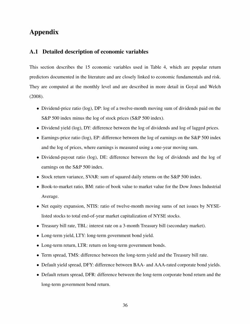
the influence of business cycle, we consider 15 monthly economic variables that are linked directly

10

to economic fundamentals and risk,6 which are the log dividend-price ratio (DP), log dividend yield

(DY), log earnings-price ratio (EP), log dividend payout ratio (DE), stock return variance (SVAR),

book-to-market ratio (BM), net equity expansion (NTIS), Treasury bill rate (TBL), long-term bond

yield (LTY), long-term bond return (LTR), term spread (TMS), default yield spread (DFY), default

return spread (DFR), inflation rate (INFL), and consumption-wealth ratio (CAY). Details on these

economic predictors are provided in the Appendix.

3. Predictive Regression Analysis

3.1 Manager sentiment and aggregate market returns

Consider the standard predictive regression model,

Rmt+1 = α +βSMS

t + εt+1, (4)

where Rmt+1 is the excess aggregate market return, i.e., the monthly return on the S&P 500 index

in excess of the risk-free rate, and SMSt is the manager sentiment index defined as the average of

the standardized aggregate manager tone extracted from conference calls and 10-Ks and 10-Qs. In

addition, for comparison, we also consider SRC, the alternative regression-combined managerial

sentiment index, and four individual tone measures. Each manager sentiment index and individual

tone measure in (4) is standardized to have zero mean and unit variance.

The null hypothesis of interest is that manager sentiment has no predictive ability, β = 0. In

this case, (4) reduces to the constant expected return model, Rmt+1 = α + εt+1. Because finance

theory suggests a negative sign on β , we test H0 : β = 0 against HA : β < 0, which is closer to

theory than the common alternative of β 6= 0. Econometrically, Inoue and Kilian (2004) encourage

6The economic variables are reviewed in Goyal and Welch (2008), and the updated data for the first 14 variables areavailable from Amit Goyal’s website, http://www.hec.unil.ch/agoyal/, and the consumption-wealth ratio is availablefrom Sydney C. Ludvigson’s website, http://www.econ.nyu.edu/user/ludvigsons/.

11

the use of the one-sided alternative hypothesis to increases the power of the test.

Several econometric issues may have an adverse impact on the statistical inferences we draw

from Equation (4). First, if a predictor is highly persistent, the OLS regression may generate

spurious results (Ferson, Sarkissian, and Simin 2003). Second, due to the well-known Stambaugh

(1999) small-sample bias, the coefficient estimate of the predictive regression can be biased in a

finite sample, which may distort the t-statistic when the predictor is highly persistent and correlated

with the excess market return. To alleviate potential concerns with these two issues, we base our

inferences on the empirical p-values that we obtain using a wild bootstrap procedure that accounts

for the persistence in predictors, correlations between the excess market return and predictor

innovations, and general forms of return distribution. 7

[Insert Table 2 about here]

Table 2 reports the in-sample estimation results of the predictive regressions (4). Panel A

provides the results for the manager sentiment index, SMS. The regression slope on SMS, β , is

−1.26, which is economically large and statistically significant at the 1% level based on the wild

bootstrap p-value, with a Newey-West t-statistic of−3.57. Therefore, SMS is a significant negative

market predictor: high manager sentiment is associated with low excess aggregate market return in

the next month. This finding is consistent with our hypothesis that SMS as a sentiment index leads

to market-wide over-valuation (under-valuation) when SMS is high (low), leading to subsequent

low (high) stock returns.

Interestingly, our finding of a negative relation between the manager sentiment index SMS

and aggregate market return is in sharp contrast with the relation at the firm-level. For example,

Loughran and McDonald (2011) find that a higher proportion of negative words from the 10-Ks

and 10-Qs is associated with more negative excess returns in the filing period at the firm level.

7The details of the wild bootstrap procedure is untabulated but available on request. Amihud and Hurvich(2004), Lewellen (2004), Campbell and Yogo (2006), and Amihud, Hurvich, and Wang (2009) develop predictiveregression tests that explicitly account for the Stambaugh small-sample bias. Inferences based on these procedures arequalitatively similar to those based on the bootstrap procedure.

12

Price, Doran, Peterson, and Bliss (2012) also find a positive association between the conference

call tone and abnormal returns at the firm level. Therefore, the firm-level tone effects do not extend

to the market level and our aggregate evidence is more consistent with the managerial sentiment

explanation rather than fundamental information explanation. This finding is consistent with

Hirshleifer, Hou, and Teoh (2009) who also find opposite relationship for the return predictability

of accruals and cash flows at the market level versus the firm level.

Economically, the regression coefficient suggests that a one-standard deviation increase in

SMS is associated with a −1.26% decrease in expected excess market return for the next month.

Recall that the average monthly excess market return during our sample period is 0.76% (α in

(4) and Table 2), thus the slope of −1.26% implies that the expected excess market return based

on SMS varies by about 1.5 times larger than its average level, which signals strong economic

significance (Cochrane 2011). In addition, SMS generates a large R2 of 9.75%. If this level

of predictability can be sustained out-of-sample, it will be of substantial economic significance

(Kandel and Stambaugh 1996). Indeed, Campbell and Thompson (2008) show that, given the

large unpredictable component inherent in the monthly market returns, a monthly out-of-sample

R2 statistic of 0.5% can generate significant economic value. This point will be analyzed further in

Section 4.1.

Panel B provides the estimation results for the regression-combined manager sentiment index,

SRC. The regression slope on SRC is −1.28, with a Newey-West t-statistic of −3.67, which is

slightly larger than that of SMS in Panel A, suggesting that the optimally-weighted SRC can further

improve the return predictability upon SMS, in the in-sample fitting context. The R2 of 10.3% is

also slightly larger than the 9.75% reported in Panel A for SMS. However, Rapach, Strauss, and

Zhou (2009) show that the sophisticated optimally weighted forecast may underperform the naive

equally-weighted forecast in a more realistic out-of-sample setting due to parameter uncertainty

and model instability. We will show later in Sections 4.1 and 4.2 that this is also true in our case

here.

13

For comparison, Panel C of Table 2 reports the predictive abilities of four individual aggregate

tone measures separately. Both SCC, the equally-weighted average conference call tone, and SFS,

the equally-weighted average financial statement tone are significant negative return predictors,

consistent with the theoretical predictions. SFS has relatively larger in-sample predictability, with

an R2 of 8.10% vis-a-vis 4.05% of SCC, consistent with its higher weight in forming the SRC

index. As a robustness check, we also examine the forecasting power of value-weighted average

conference call tone, SCCv, and value-weighted average financial statement tone, SFSv. We detect

significant negative return predictability again, but the forecasting power is weaker than those of the

corresponding equally-weighted tone measures. The finding is consistent with Baker and Wurgler

(2006) that since small firms are hard to value and difficult to arbitrage, they are more sensitive

to sentiment than large firms. Most importantly, we observe that SMS consistently beats all the

individual tone measures, confirming Baker and Wurgler (2006, 2007) that a composite sentiment

index is more desirable than individual proxies.

From an economic point of view, while the overall R2 is interesting, it is also important to

analyze the predictability during business-cycles to better understand the fundamental driving

forces. Following Rapach, Strauss, and Zhou (2010) and Henkel, Martin, and Nardari (2011),

we compute the R2 statistics separately for economic recessions (R2rec) and expansions (R2

exp),

R2c = 1− ∑

Tt=1 Ic

t (εi,t)2

∑Tt=1 Ic

t (Rmt − Rm)2

c = rec, exp (5)

where Irect (Iexp

t ) is an indicator that takes a value of one when month t is in an NBER recession

(expansion) period and zero otherwise; εi,t is the fitted residual based on the in-sample estimates

of the predictive regression model in (4); Rm is the full-sample mean of Rmt ; and T is the number

of observations for the full sample. Note that, unlike the full-sample R2 statistic, the R2rec and R2

exp

statistics can be both positive or negative.

Columns 6 and 7 of Table 2 report the R2rec and R2

exp statistics. Panels A and B show that

the return predictability is concentrated over recessions for the manager sentiment indexes SMS

14

and SRC. For example, over recessions, SMS has a large R2rec of 21.4%. In contrast, over

expansions, SMS has a much smaller R2exp of 0.74%. Panel C shows that, consistent with the

manager sentiment indexes, the individual tone measures also present much stronger predictability

during recessions vis-a-vis expansions. In summary, the return predictability of manager sentiment

is concentrated over recessions, consistent with Huang, Jiang, Tu, and Zhou (2015) for investor

sentiment indexes and Rapach, Strauss, and Zhou (2010) and Henkel, Martin, and Nardari (2011)

for other macroeconomic variables.

In the last two columns of Table 2, we divide the whole sample into high and low sentiment

periods to investigate the possible economic sources of the return predictability of SMS. Following

Stambaugh, Yu, and Yuan (2012), we classify a month as high (low) sentiment if the manager

sentiment level in the previous month is above (below) its median value for the sample period,

and compute the R2high and R2

low statistics for the high and low sentiment periods, respectively, in a

manner similar to (5).

Empirically, we find that the predictive power of SMS in Panel A is fairly large during both high

sentiment and low sentiment periods, although the predictability is stronger during high sentiment

periods. For example, over high sentiment periods, SMS has an R2high of 12.9%. In contrast, over

low sentiment periods, SMS has an smaller R2low of 6.93%. For the individual tone measures,

Panel C reports that the predictability of SFS is stronger during high sentiment periods, but SCC

displays stronger predictability during low sentiment periods. Comparing Panels A and C, the

more balanced forecasting performance of SMS over high and low sentiment periods is potentially

due to the fact that SMS summarizes information in both tone measures SCC and SFS, which have

stronger predictive power in low and high sentiment periods, respectively. In short, consistent with

Shen and Yu (2013) and Huang, Jiang, Tu, and Zhou (2015) for investor sentiment, we also find

that manager sentiment’s predictive power is stronger over high sentiment periods, during which

mispricing is more likely due to short-sale constraints.

15

3.2 Predictability with longer horizons

Although we perform most of our empirical tests on manager sentiment over the usual one month

horizon, in this subsection, we investigate its forecasting power over longer horizons. Manager

sentiment is highly persistent and long-term in nature and hence may have a long run effect

on stock market. In addition, due to limits of arbitrage, mispricings from manager sentiment

may not be eliminated completely by arbitrageurs over a short horizon. Brown and Cliff (2004,

2005) show that survey-based investor sentiment has significant return predictability over long run

horizons exceeding one year. Baker, Wurgler, and Yuan (2012) show that global sentiment in year

t− 1 predicts significantly the following 12 month country-level market returns over 1980–2005.

Huang, Jiang, Tu and Zhou (2015) show that aligned investor sentiment SHJTZ presents significant

forecasting power for up to a one-year forecasting horizon.

[Insert Table 3 about here]

Table 3 reports the in-sample estimation results of the manager sentiment index SMS on the

excess market return over horizons from one month to three years. For comparison, we also

report results for the regression-combined manager sentiment SRC. Panel A shows that SMS

can significantly predict the long run excess market return for up to three years. The in-sample

forecasting power increases as the horizon increases and then declines. Specifically, the in-sample

R2 of SMS peaks at the 9-month forecasting horizon of 27.1%; the absolute value of the regression

coefficient on SMS generally increases as horizon increases and begins to stabilizes at 24 months.

At the annual horizon, a one-standard deviation positive shock to SMS predicts a −8.58% decrease

in the aggregate stock market return over the next one year. In addition, we obtain qualitatively

similar findings for SRC in Panel B.

In sum, the manager sentiment index SMS significantly predicts stock market returns not only

at the usual one month horizon but also over long run horizons up to three years into the future,

with a peak at the 9-month horizon.

16

3.3 Comparison with economic predictors

In this subsection, we compare the forecasting power of the manager sentiment index SMS with

economic predictors and examine whether its forecasting power is driven by omitted economic

variables related to business cycle fundamentals or changes in macroeconomic risks.

First, we consider the predictive regression on a single economic variable,

Rmt+1 = α +ψZk

t + εt+1, k = 1, ...,16, (6)

where Zkt is one of the 15 individual economic variables described in Section 2.2 and in the

Appendix or the ECON factor which is the first principal component (PC) extracted from the

15 individual economic variables.

[Insert Table 4 about here]

Panel A of Table 4 reports the estimation results for (6). Out of the 15 individual economic

predictors, only stock return variance (SVAR), net equity expansion (NTIS), Treasury bill rate

(TBL), and long-term yield (LTY) exhibit significant predictive abilities for the market at the 10%

or better significance levels. Among these four significant economic variables, three of them have

R2s larger than 1.5% (SVAR, NTIS, and LTY), and one has an R2 larger than 5% (SVAR). The

last row of Panel A shows that the ECON factor, the first PC extracted from the 15 economic

variables, is insignificant in forecasting excess market return, with a small R2 of only 0.12%.

Hence, SMS outperforms all 15 individual economic predictors and the PC common factor, ECON,

in forecasting the monthly excess market returns in-sample.

We then investigate whether the forecasting power of SMS remains significant after controlling

for economic predictors. To analyze the incremental forecasting power of SMS, we conduct the

following bivariate predictive regressions based on SMSt and each economic variable, Zk

t ,

Rmt+1 = α +βSMS

t +ψZkt + εt+1, k = 1, ...,16. (7)

17

The coefficient of interest is the regression slope β on SMSt . We test H0 : β = 0 against HA : β < 0

based on the wild bootstrapped p-values.

Panel B of Table 4 shows that the estimates of the slope β in (7) range from −1.10 to

−1.95, all of which are negative and economically large, in line with the results in the earlier

predictive regression (4) reported in Table 2. More importantly, β remains statistically significant

at the 1% or better level when augmented by the economic predictors. The R2s in (7) range

from 9.83% to 15.3%, which are substantially larger than those reported in Panel A based on

the economic predictors alone. These results demonstrate that the return predictability of the

manager sentiment index SMS is not driven by macroeconomic fundamentals and it contains sizable

sentiment forecasting information complementary to what is contained in the economic predictors.

3.4 Comparison with alternative sentiment indexes

In this subsection, we empirically compare the manager sentiment index SMS with five alternative

sentiment indexes documented in the literature, and examine whether the forecasting power of

SMS is a substitute for or is complementary to investor sentiment. Theoretically, a priori, there

are no strong reasons to believe that investor sentiment will perform better or worse than manager

sentiment in predicting the stock market. As insiders, managers are better informed about their

firms than outside investors and have the first-hand ability to create value for firms. At the same

time, recent research shows that managers are also often subject to cognitive biases and may not

be fully rational. Therefore, while the literature generally exclusively focus on investor sentiment

in forecasting stock returns, in practice, investor and manager sentiment likely coexist.

We run the the following predictive regressions of monthly excess market return (Rmt+1) on the

lagged manager sentiment index, SMS, with controls for alternative sentiment indexes, Skt ,

Rmt+1 = α +βSMS

t +δSkt + εt+1, k = BW,HJTZ,MCS,CBC,FEARS, (8)

18

where SBW denotes the Baker and Wurgler (2006) investor sentiment index, SHJTZ denotes the

Huang, Jiang, Tu, and Zhou (2015) aligned investor sentiment index, SMCS denotes the University

of Michigan consumer sentiment index, SCBC denotes the Conference Board consumer confidence

index, and SFEARS denotes the Da, Engelberg, and Gao (2015) FEARS investor sentiment index

(over the sample period 2004:07−2011:12 due to data constraints). Detailed descriptions of these

alternative sentiment indexes are provided in Section 2.2. To test the incremental forecasting

information contained in SMSt , we test H0 : β = 0 against HA : β < 0 based on the wild bootstrapped

p-values.

[Insert Table 5 about here]

As a benchmark, the first column of Table 5 shows that the manager sentiment index SMS is a

significant negative predictor for the market, with a large R2 of 9.75%. In the second column, the

widely used Baker and Wurgler (2006) investor sentiment index SBW has an in-sample R2 of 5.11%,

which is much lower than the predictability of SMS, although SBW is indeed a significant negative

predictor for the excess market return. Interestingly, in the third column, when including both SMS

and SBW jointly as return predictors in a bivariate predictive regression, SMS remains significant

but SBW becomes insignificant, and the R2 of the bivariate regression is equal to 10.3%, which is

similar to that of using SMS alone. These findings are consistent with the high correlation of 0.53

between SMS and SBW in Table 1, indicating that SMS empirically dominates SBW in forecasting

the stock market.

The fourth column of Table 5 shows that the Huang, Jiang, Tu and Zhou (2015)’s aligned

investor sentiment index SHJTZ, which is an alternative investor sentiment index generated by

exploring the the same six stock market-based sentiment proxies of Baker and Wurgler (2006) more

efficiently, generates a larger R2 of 8.45%, with statistical and economic significance. However,

SHJTZ’s predictability, in term of in-sample R2, is still smaller than that of SMS, although the

difference is economically small. More interesting, the fifth column shows that when combining

SMS together with SHJTZ, the bivariate predictive regression generates an in-sample R2 of 16.7%,

19

almost equal to the sum of the individual R2s of the univariate regressions, revealing that the

predictive power of the manager sentiment index SMS and the aligned investor sentiment index

SHJTZ are almost perfectly complimentary to each other, consistent with their low correlation in

Table 1.

The sixth to eleventh columns of Table 5 show that the return predictability of the University

of Michigan consumer sentiment index (SMCS), the Conference Board consumer confidence index

(SCBC), and the Da, Engelberg, and Gao (2015)’s FEARS investor sentiment index (SFEARS) are

smaller than that of SMS, ranging from 0.26% to 2.71%. Most importantly, they each become

statistically insignificant when controlling for SMS in bivariate regressions, while SMS remains

consistently significant and negative. In the last column, we run a kitchen-sink regression that

includes all the sentiment indexes in one long regression. We find that SMS remains statistically

significant and economically large, while the coefficients on the other sentiment indexes become

more volatile due to serious multicollinearity problem.

In short, the manager sentiment index SMS contains additional sentiment information beyond

exiting sentiment indexes in forecasting the stock market. In addition, SMS is almost perfectly

complimentary to the aligned investor sentiment index SHJTZ in forecasting.

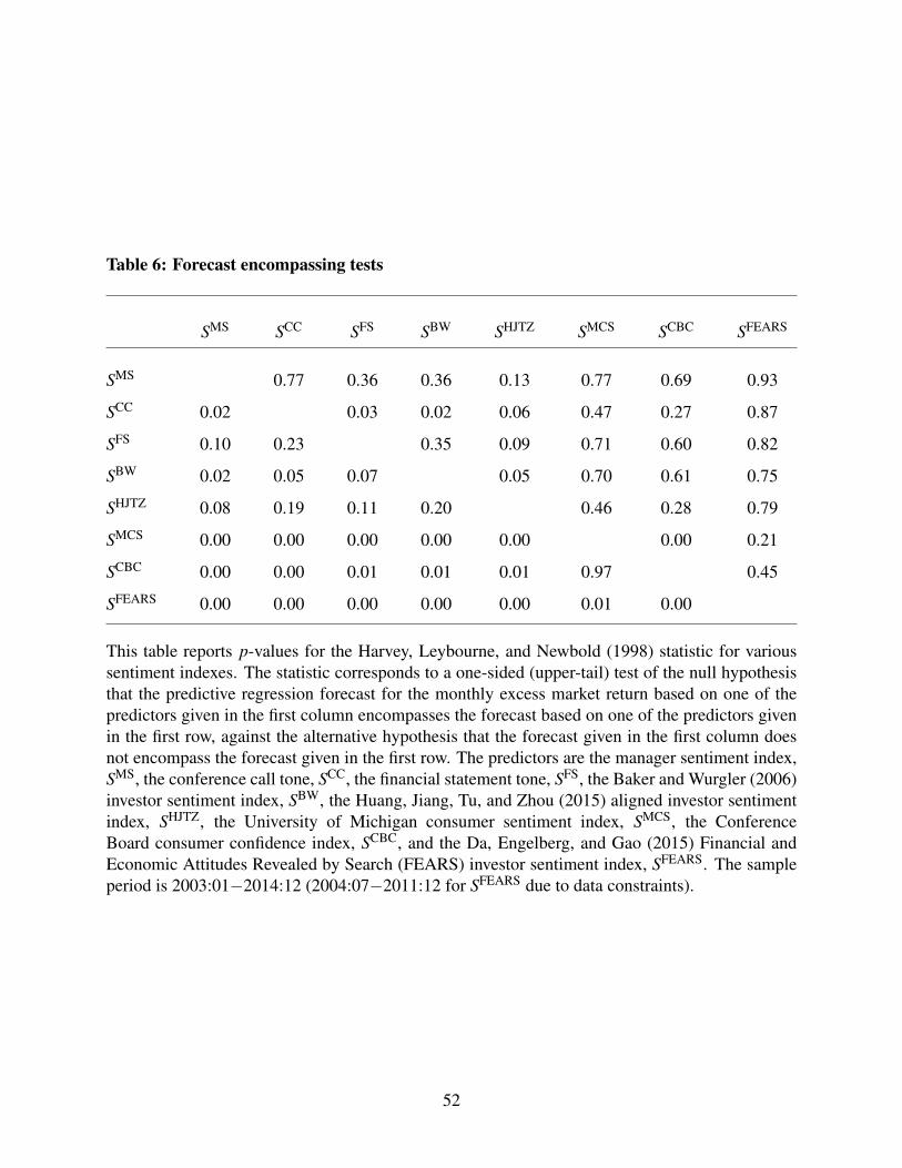
3.5 Forecast encompassing test

To further assess the relative information content between the manager sentiment index SMS and

the other five alternative sentiment indexes, we conduct a forecast encompassing test. Harvey,

Leybourne, and Newbold (1998) develop a statistic for testing the null hypothesis that a given

forecast contains all of the relevant information found in a competing forecast (i.e., the given

forecast encompasses the competitor) against the alternative that the competing forecast contains

relevant information beyond that in the given forecast.

[Insert Table 6 about here]

20

Table 6 reports p-values for the Harvey, Leybourne, and Newbold (1998) forecast encom-

passing test. The first row of Table 6 shows that the manager sentiment index SMS encompasses

the two individual tone measures as well as the five alternative sentiment indexes at conventional

significance levels (but marginally for SHJTZ); however,the individual tone components SCC and SFS

fail to do so. These findings confirm the potential gains in efficiently combining individual tone

measures into a composite manager sentiment index to fully make use of relevant information,

as discussed in Table 2. In addition, the fourth to eighth rows of Table 6 show that none of the

five alternative sentiment indexes can significantly encompass SMS and its components SCC and

SFS, suggesting that the manager sentiment index SMS contains incremental sentiment forecasting

information beyond existing sentiment measures.

4. Economic Value

4.1 Out-of-sample R2OS

In this section, we investigate the out-of-sample forecasting performance of the manager sentiment

index. Goyal and Welch (2008), among others, argue that out-of-sample tests are more relevant for

investors and practitioners for assessing genuine return predictability in real time, although the in-

sample predictive analysis provides more efficient parameter estimates and thus more precise return

forecasts. In addition, out-of-sample tests are much less affected by the econometrics issues such

as the over-fitting concern, small-sample size distortion and the Stambaugh bias than in-sample

regressions (Busetti and Marcucci, 2012). Hence, we investigate the out-of-sample predictive

performance of the manager sentiment index, SMS.

The key requirement for out-of-sample forecasts at time t is that we can only use information

available up to t to forecast stock returns at t + 1. Following Goyal and Welch (2008), and

many others, we run the out-of-sample predictive regressions recursively on each lagged manager

21

sentiment measure,

Rmt+1 = αt + βtSk

1:t;t (9)

where αt and βt are the OLS estimates from regressing {Rms+1}

t−1s=1 on a constant and a recursively

estimated sentiment measure {Sk1:t;s}

t−1s=1. Similar to our in-sample analogues in Table 2, we

investigate the out-of-sample forecasting performance of the recursively estimated manager

sentiment index, SMS, the regression-combined manager sentiment index, SRC, the conference call

tone, SCC, and the financial statement tone, SFS. In addition, we also consider the combination

forecast of manager sentiment proxies, SC, that is widely used in the forecasting literature and

often beats sophisticated optimally estimated forecasting weights (Timmermann, 2006). Rapach,

Strauss, and Zhou (2009) show that a simple equally-weighted average of univariate regression

forecasts can consistently predict the market risk premium. It is hence of interest to see how well it

performs in the context of using the two individual tone measures. For comparison purse, we also

examine the out-of-sample forecasting performance of the five alternative sentiment indexes as in

Table 5.

Let p be a fixed number chosen for the initial sample training, so that the future expected

return can be estimated at time t = p+1, p+2, . . . ,T . Hence, there are q (= T − p) out-of-sample

evaluation periods. That is, we have q out-of-sample forecasts: {Rmt+1}

T−1t=p . Specifically, we use the

data over 2003:01 to 2006:12 as the initial estimation period, so that the forecast evaluation period

spans over 2007:01 to 2014:12. The length of the initial in-sample estimation period balances

having enough observations for precisely estimating the initial parameters with the desire for a

relatively long out-of-sample period for forecast evaluation.8

We evaluate the out-of-sample forecasting performance based on the widely used Campbell

and Thompson (2008) R2OS statistic. The R2

OS statistic measures the proportional reduction in

mean squared forecast error (MSFE) for the predictive regression forecast relative to the historical

8Hansen and Timmermann (2012) and Inoue and Rossi (2012) show that out-of-sample tests of predictive abilityhave better size properties when the forecast evaluation period is a relatively large proportion of the available sample,as in our case.

22

average benchmark,

R2OS = 1−

∑T−1t=p (R

mt+1− Rm

t+1)2

∑T−1t=p (R

mt+1− Rm

t+1)2, (10)

where Rmt+1 denotes the historical average benchmark corresponding to the constant expected return

model (Rmt+1 = α + εt+1),

Rmt+1 =

1t

t

∑s=1

Rms . (11)

Goyal and Welch (2008) show that the historical average is a very stringent out-of-sample

benchmark, and individual economic variables typically fail to outperform the historical average.

The R2OS statistic lies in the range (−∞,1]. If R2

OS > 0, then the forecast Rmt+1 outperforms the

historical average Rmt+1 in terms of MSFE.

We test the statistical significance of R2OS using the MSFE-adjusted statistic of Clark and West

(2007) (MSFE–adj statistic). It tests the null hypothesis that the historical average MSFE is

less than or equal to the predictive regression forecast MSFE against the one-sided (upper-tail)

alternative hypothesis that the historical average MSFE is greater than the predictive regression

forecast MSFE, corresponding to H0: R2OS ≤ 0 against HA : R2

OS > 0. Clark and West (2007) show

that this test has an asymptotically standard normal distribution when comparing forecasts from

the nested models. Intuitively, under the null hypothesis that the constant expected return model

generates the data, the predictive regression model produces a noisier forecast than the historical

average benchmark because it estimates slope parameters with zero population values. We thus

expect the benchmark model’s MSFE to be smaller than the predictive regression model’s MSFE

under the null. The MSFE-adjusted statistic accounts for the negative expected difference between

the historical average MSFE and predictive regression MSFE under the null, so that it can reject

the null even if the R2OS statistic is negative.

[Insert Table 7 about here]

Panel A of Table 7 shows that the manager sentiment index SMS exhibits strong out-of-sample

predictive ability for the aggregate market, with an R2OS of 8.38%. The Clark and West (2007)

23

MSFE–adj statistic of SMS is 2.55, suggesting that the MSFE of SMS is significantly smaller than

that of the historical average at the 1% or better significance level. The R2OS of SMS is economically

large and exceeds substantially all the other R2OSs in Table 7, including all other manager sentiment

measures in Panel A and all five alternative sentiment indexes in Panel B. The two manager tone

components SCC and SFS have significant forecasting power, with R2OSs of 1.77% and 6.85%,

respectively, both of which are smaller than the predictability of SMS, indicating the forecasting

gains that result from combining information from two tone measures into a composite manager

sentiment index. In addition, the fourth and fifth columns of Table 7 show that the predictability

of the manager sentiment index SMS and its individual tone measures SCC and SFS is concentrated

over recessions, confirming our earlier in-sample findings in Table 2.

The recursively estimated regression-combined manager sentiment index, SRC, generates a pos-

itive R2OS of 5.70%, hence, while the sophisticated optimally-estimated SRC slightly outperforms

the equally-weighted index SMS in the in-sample fitting context (see Table 2), it substantially

underperfoms SMS in the more realistic out-of-sample setting. Consistent with Rapach, Strauss,

and Zhou (2010), the combination forecast SC generates a large R2OS of 7.94%, with statistical

significance at the 5% level. These findings are largely consistent with Goyal and Welch (2008)

that while sophisticated estimated models may have good in-sample fitting, their out-of-sample

performance tends to be worse due to large estimation error.

For comparison, Panel B of Table 7 shows the out-of-sample performance of the five alternative

sentiment indexes. Among the five indexes, two investor sentiment indexes SBW and SHJTZ are

positive and significant, with R2OSs of 4.54% and 3.14%, respectively. The R2

OSs of other three

sentiment indexes SMCS, SCBC, and SFEARS are negative, indicating forecasting loss relative to the

historical average benchmark. Nevertheless, all the R2OSs of the alternative sentiment indexes are

substantially lower than the R2OS of manager sentiment index SMS.

In summary, this section shows that the manager sentiment SMS displays strong out-of-sample

forecasting power for the aggregate stock market. In addition, SMS substantially outperforms all

24

the other manager sentiment measures and alternative investor sentiment indexes documented in

the literature in an out-of-sample setting, consistent with the results of our in-sample regression

analysis in Section 2.

4.2 Asset allocation implications

In this section, we further examine the economic value of stock return predictability of the manager

sentiment index SMS from an asset allocation perspective. Following Kandel and Stambaugh

(1996), Campbell and Thompson (2008) and Ferreira and Santa-Clara (2011), among others, we

compute the certainty equivalent return (CER) gain and Sharpe Ratio for a mean-variance investor

who optimally allocates across equities and the risk-free asset using the out-of-sample predictive

regression forecasts.

At the end of period t, the investor optimally allocates

wt =1γ

Rmt+1

σ2t+1

(12)

of the portfolio to equities during period t + 1, where γ is the risk aversion coefficient of five,

Rmt+1 is the out-of-sample forecast of excess market return, and σ2

t+1 is the variance forecast. The

investor then allocates 1−wt of the portfolio to risk-free bills, and the t+1 realized portfolio return

is

Rpt+1 = wtRm

t+1 +R ft+1, (13)

where R ft+1 is the risk-free return. Following Campbell and Thompson (2008), we assume that the

investor uses a five-year moving window of past monthly returns to estimate the variance of the

excess market return and constrains wt to lie between 0 and 1.5 to exclude short sales and to allow

for at most 50% leverage.

The CER of the portfolio is

CERp = µp−0.5γσ2p , (14)

25

where µn and σ2n are the sample mean and variance, respectively, for the investor’s portfolio over

the q forecasting evaluation periods. The CER gain is the difference between the CER for the

investor who uses a predictive regression forecast of market return generated by (9) and the CER

for an investor who uses the historical average forecast (11). We multiply this difference by 12 so

that it can be interpreted as the annual portfolio management fee that an investor would be willing

to pay to have access to the predictive regression forecast instead of the historical average forecast.

In addition, we also calculate the monthly Sharpe ratio of the portfolio, which is the mean

portfolio return in excess of the risk-free rate divided by the standard deviation of the excess

portfolio return. To examine the adverse effect of transaction costs, we also consider the case

of 50bps transaction costs, which is generally considered as a relatively high number.

[Insert Table 8 about here]

Table 8 shows that the manager sentiment index SMS generates large economic gains for the

mean-variance investor, consistent with its large R2OS statistics in Table 7. Specifically, SMS has a

large positive annualized CER gain of 7.92%, indicating that an investor with a risk aversion of

five would be willing to pay an annual portfolio management fee up to 7.92% to have access to

the predictive regression forecasts based on SMS instead of using the historical average forecast.

The CER gain remains economically large after accounting for transaction costs, with a net-of-

transactions-costs CER gain of 7.86%. The monthly Sharpe ratio of SMS is about 0.17, which is

much higher than the market Sharpe ratio,−0.02, over the same sample period with a buy-and-hold

strategy.

The rest of Panel A shows that all the other manager sentiment or tone measures also generate

large economic gains for the investor. The annualized CER gains vary from 6.64% (SRC) to 10.6%

(SFS), and the net-of-transactions-costs CER gains vary from 6.56% (SRC) to 10.5% (SFS). In

addition, all the monthly Sharpe ratios are also economically large, in the range of 0.13 (SRC and

SCC) to 0.22 (SFS).

Panel B of Table 8 shows that, out of the five alternative sentiment indexes, the two investor

26

sentiment indexes SBW and SHJTZ generate large economic gains for the investor, while the gains

from the other three indexes are limited. Specifically, without transaction costs, SBW and SHJTZ

generate both large CER gains (9.06% for SBW and 8.79% for SHJTZ) and large Sharpe ratios (0.19

for SBW and 0.18 for SHJTZ), and the economic gains remain large after accounting for transaction

costs. However, while SMCS and SFEARS can generate fairly large CER gains (4.17% for SMCS and

5.80% for SFEARS), their Sharpe ratios are low, 0.03 and 0.01, respectively. SMCS only generates

small CER gain of 0.62% and a negative Sharpe ratio of −0.03.

Overall, Table 8 demonstrates that the manager sentiment index SMS can generate sizable

economic value for an investor from an asset allocation perspective. The results are robust to

common levels of transaction costs.

5. Manager Sentiment and Aggregate Earnings

In this section, we investigate the forecasting power of the manager sentiment index SMS for

future aggregate earnings growth. Thus far we have focused on forecasting market returns with

manager sentiment; however, stock prices are determined not only by discount rates but also by

expectations about future cash flows. Therefore, the negative return predictability of the manager

sentiment index may come from investors’ biased beliefs about future earnings unjustified by

economic fundamentals in hand (e.g., Bower 1981; Johnson and Tversky 1983; Wright and Bower

1992; Baker and Wurgler 2007). Specifically, when manager sentiment is high (low), the market

may have overly optimistic (pessimistic) expectations for future earnings, leading to overvaluation

(undervaluation) and subsequent low (high) stock returns.

Our empirical analysis focuses on forecasting future aggregate earnings growth, which has

been widely examined and used in similar studies in the literature (e.g., Campbell and Shiller

1988; Fama and French 2000; Menzly, Santos, and Veronesi 2004; Lettau and Ludvigson 2005;

Cochrane 2008, 2011; Binsbergen and Koijen 2010; Huang, Jiang, Tu, and Zhou 2015). We

27

employ the following predictive regressions,

EGt→t+12 = α +βSMSt +ψE/Pt +δEGt +υt→t+12, (15)

where EGt→t+12 is the annual growth rate of twelve-month moving sums of aggregate earnings on

the S&P 500 index, which is available from Robert Shiller’s website and from Goyal and Welch

(2008). Following previous studies, we include controls for the lagged earnings-to-price ratio

(E/Pt) and lagged earnings growth (EGt), and focus on annual horizon data to avoid spurious

earnings growth predictability arising from within-year seasonality.9 We are interested in the

regression slope β , and test H0 : β = 0 against HA : β < 0, to examine whether the manager

sentiment index , SMSt , contains information about future aggregate earnings growth.

[Insert Table 9 about here]

Table 9 reports the estimation results of forecasting annual aggregate earnings growth in

(15). The first two columns show that manager sentiment SMS contains significant negative

forecasting power for future aggregate earnings growth EGt→t+12. According to the first column,

the regression slope estimate on SMS for EGt→t+12 is −0.46, with a Newey-West t-statistic of

−2.26. Hence, a one-standard deviation increase in SMS is associated with a −46% decrease in

EGt→t+12 for the next year, revealing that aggregate earnings growth is highly predictable with

manager sentiment over our sample period. This point is further confirmed by the large R2 of

35.6% for the univariate predictive regression for EGt→t+12 with SMS.

The negative predictability of manager sentiment for next-year aggregate earnings growth is

consistent with our previous finding on negative market return predictability reported in Section 3.1

and Table 2. The finding suggests that aggregate manager sentiment index captures systematically

biased beliefs about future cash flows rather than fundamental information. The aggregate-level

9In unreported tables, we find similar but weaker results for aggregate dividend growth, which is consistent withFama and French (2001) that there is a steep-downward trend in the fraction of U.S. firms paying dividends, and thatthe dividends are subject to smoothing.

28

evidence contrasts with the positive association between firm-level manager sentiment (tone) and

subsequent firm-level earnings documented in Feldman, Govindaraj, Livnat, and Segal (2010), Li

(2010), Loughran and McDonald (2011), and Price, Doran, Peterson, and Bliss (2012). However,

the finding is consistent with Huang, Jiang, Tu, and Zhou (2015) which find negative negative

association between sentiment and aggregate earnings growth for the aligned investor sentiment

index, and Hribar and McInnis (2012) which find negative association between sentiment and

analysts’ earnings forecasts errors for the Baker and Wurgler’s investor sentiment index.

In the second column of Table 9, we further control for lagged earnings-to-price ratio (E/Pt)

and annual earnings growth rate (EGt), and find that the aggregate earnings growth predictability

of SMS remains robust when controlling for these two aggregate earnings related controls. In

addition, both lagged earnings-to-price ratio (E/Pt) and lagged annual earnings growth (EGt)

are insignificant negative predictors for EGt→t+12, indicating weak mean-reversion in aggregate

earnings growth.

For comparison, in the third to last columns, we examine the aggregate earnings growth

predictably of the regression-combined manager sentiment index, SRC, the conference call tone,

SCC, and the financial statement tone, SFS. We find that all of these alternative manager

sentiment measures present significant negative predictive power for EGt→t+12, consistent with

SMS. Specifically, SRC has a regression slope of −0.42 and an R2 of 29.8%, which is statistically

significant but smaller than the predictability of SMS. Both tone measures of SCC and SFS generate

large earnings growth predictability, with R2s of 35.9% and 13.7%, respectively. Thus, SCC

contains relatively greater information content about future aggregate earnings growth than SFS,

which is in sharp contrast with their relative importance in forecasting aggregate market returns,

again confirming their complementary roles.

In short, Table 9 shows that manager sentiment is a negative indicator for future cash flows,

and high manager sentiment is negatively associated with next-year aggregate earnings growth.

Our findings hence suggest that, when manager sentiment is high, the market suffers from

29

overly optimistic belief about future aggregate cash flow (earnings) growth, which causes market

overvaluation. When bad cash flows news are gradually revealed to investors, the overvaluation

diminishes and stock prices fall, leading to low low future returns.

6. Manager Sentiment and Characteristic Portfolio Returns

As highlighted by Shleifer and Vishny (1997), Baker and Wurgler (2006, 2007) and Stambaugh,

Yu, and Yuan (2012), firms that are hard to value tend to be more sensitive to irrational speculation

from sentiment investors. Moreover, the sentiment-driven misvaluation is more likely to sustain in

the presence of limits to arbitrage, when informed arbitrageurs move slowly to exploit the profit

opportunities. Therefore, manager sentiment’s forecasting power may also have cross-sectional

effects, and may be stronger among stocks that are more speculative, difficult to value, or hard to

arbitrage, similar to investor sentiment. In this section, we explore the cross-sectional variation

of manager sentiment’s effects on stock returns. These cross-sectional tests not only help to

strengthen our previous findings for aggregate stock market predictability, but also help to enhance

our understanding for the economic channels through which manager sentiment impacts asset

prices.

Following Baker and Wurgler (2006, 2007), we consider 11 well-documented decile portfolios

formed on single sorting on firm characteristics, including beta, idiosyncratic volatility, firm age,

size, earnings-to-book equity ratio (profit), dividends-to-book equity ratio (dividend), PPE-to-total

asset ratio (fixed asset), R&D-to-total asset ratio (R&D), book-to-market ratio (B/M), dividends-to-

price ratio (D/P), and total asset growth (investment), which are related to subjectivity of valuation

and limits to arbitrage.

• Beta, the Scholes-Williams (1977) beta for daily common stock returns over a year available

from CRSP. Baker, Bradley, and Wurgler (2011) argue that high-beta stocks are more prone

to speculate and are more difficult to arbitrage due to institutional frictions.

30

• Idiosyncratic volatility, the standard deviation of the residuals from regressing daily stock

returns on market returns over a year. Barberis and Xiong (2010) and Baker, Bradley, and

Wurgler (2011) suggest that high-volatility stocks are more speculative, and Wurgler and

Zhuravskaya (2002) and Stambaugh, Yu, and Yuan (2015) use idiosyncratic volatility as a

proxy for limits to arbitrage.

• Age, the number of years listed in Compustat. Baker and Wurgler (2006, 2007) argue that

young firms are more difficult to value and are hard to arbitrage.

• Size, the price per share multiplied by the number of shares outstanding, available from Ken

French’s website. Small firms are difficult to arbitrage.

• Profit, earnings (defined as revenues minus cost of goods sold, interest expense, and selling,

general, and administrative expenses) divided by book equity available from Ken French’s

website. Baker and Wurgler (2006, 2007) argue that the valuation of unprofitable firms is

difficult and they have higher limits to arbitrage.

• Dividend, total dividends divided by book equity. Similar to earnings, non-dividend-paying

stocks are speculative and difficult to arbitrage.

• Fixed asset, property, plant, and equipment (PPE) divided by total assets as a proxy for asset

tangibility. Baker and Wurgler (2006, 2007) argue that firms with high fixed asset are hard

to value and are speculative.

• R&D, research and development expense (R&D) divided by total assets. Similar to fixed

assets, R&D proxies for asset intangibility, and firms with high R&D are hard to value.

• B/M, the book to market equity ratio available from Ken French’s website. Baker and

Wurgler (2006, 2007) argue that low B/M firms have high growth opportunities, high B/M

firms are distressed, and firms in the middle are stable. Both high growth firms (low B/M)

and distressed firms (high B/M) are hard to value and difficult to arbitrage.

• D/P, the total dividends to market equity ratio available from Ken French’s website. Similar

to B/M, low D/P firms have high growth opportunities, while high D/P firms are distressed.

• Investment, the year-to-year change in total assets divided by lagged total assets available

31

from Ken French’s website. High-investment firms are high growth stocks, while low-

investment firms are distressed.

We form value-weighted monthly decile portfolios based on the above firm characteristics.

Decile 1 refers to firms in the lowest decile, decile 5 refers to firms in the middle, and decile

10 refers to firms in the highest decile. We then look for patterns in the cross-section of decile

portfolios conditional on manager sentiment. We expect that, as in Baker and Wurgler (2006,

2007), manager sentiment should present stronger forecasting power for stocks that are speculative

and hard to value (i.e., high beta, high volatility, young, unprofitable, non-dividend-paying, with

high intangible assets, and high growth), and/or difficult to arbitrage (i.e., high beta, high volatility,

young, small, unprofitable, high growth, and distressed).

[Insert Figure 2 about here]

Figure 2 reports the average monthly excess returns for two-way sorts based on the 11 firm

characteristics and manager sentiment over the sample period 2003:01–2014:12. To identify the

cross-sectional effects of manager sentiment on stock returns, we classify monthly returns as

following periods of high or low manager sentiment relative to its median value. We then calculate

average returns separately over high and low manager sentiment period and the return differences

between high and low manager sentiment periods.

The results in Figure 2 strongly support our hypothesis that the effects of manager sentiment on

stock prices are stronger among stocks that are speculative, hard to value, or difficult to arbitrage.

Panel A shows that when sentiment is low, high beta firms earn substantially higher future returns

than those with low beta; however, when sentiment is high, high beta firms earn surprisingly lower

returns. These findings suggest that aggregate manager sentiment more strongly impacts high beta

stocks than those low beta ones, consistent with our hypothesis and Baker and Wurgler (2006).

These findings also indicate that the low beta anomaly only exists during high manager sentiment

periods, when misvaluation is more likely, consistent with Stambaugh, Yu, and Yuan (2012) and

Antoniou, Doukas, and Subrahmanyam (2015). In the rest of Figure 2, we obtain generally similar

32

findings for the other firm characteristics, and find that firms with high idiosyncratic volatility,

young age, small market cap, unprofitable, non-dividend-paying, distressed (high B/M, high D/P,

low investment), and high growth opportunities (low D/P, high investment) tend to react more

strongly to manager sentiment, with higher returns following low manager sentiment and lower

returns following periods of high manager sentiment.10

We then employ predictive regressions to further investigate the cross-sectional effects of

manager sentiment on stock returns. In Figure 2, we compute average returns for each decile

portfolio of each firm characteristic during high and low sentiment periods based on a simple binary

high-low manager sentiment classification. The predictive regression analysis, however, allows us

to incorporate the continuous information of the manager sentiment index and to conduct formal

statistical tests. We run the predictive regressions

R jt+1 = α +βSMS

t + εj

t+1, (16)

where the dependent variable R jt+1 is either the monthly excess returns or long-short return spreads

(based on sensitivity to sentiment) of the 11 decile portfolios based on firm characteristics, and

SMS is the lagged manager sentiment index, with hypothesis testing based on wild bootstrapped

p-values.

[Insert Table 10 about here]

Table 10 reports the estimation results of the predictive regressions of (16). Specifically, the

left panel of Table 10 shows that all of the regression slope estimates for SMS are significant and

negative; thus the negative predictability of manager sentiment for subsequent stock returns is

pervasive in the cross-section. More importantly, we detect large cross-sectional variation in the the

regression slope estimates β . Specifically, firms with high beta, high idiosyncratic volatility, young

10While the direction of return predictability for asset tangibility characteristics such as fixed assets and R&D areconsistent with our hypothesis in Figure 2, Table 10 shows that the patterns are statistically insignificant, similar to theresults reported in Baker and Wurgler (2006).

33

age, small market cap, low profitability, low dividends, low fixed assets, high R&D, high distress

(high B/M, high D/P, low investment), and high growth opportunities (low D/P, high investment)

are generally more predictable by manager sentiment, consistent with our hypothesis and with

the two-way sort results in Figure 2. In addition, the return predictability is economically large.

For example, the regression coefficient in the first row and decile 10 suggests that a one-standard

deviation increase in the manager sentiment index SMS is associated with a −3.55% decrease in

one-month-ahead expected excess return for high beta firms.

The right panel of Table 10 provides additional formal tests that investigate whether manager

sentiment can forecast various long-short spread portfolios formed based on sensitivity to

sentiment (10-1 for volatility, profitability and tangibility related measures; and 10-5 or 5-1 for

distress and growth measures). The results again confirm our hypothesis that speculative, hard to

value, or difficult to arbitrage stocks are more predictable by manager sentiment. For example, a

one-standard deviation increase in the manager sentiment index SMS is associated with a −2.34%

decrease in the return spread between the high beta and low beta stocks (10-1), with statistical

significance at the 1% level. Therefore, manager sentiment has a significantly stronger impact for

high beta stocks than low beta stocks. We obtain similar findings for other characteristics including

idiosyncratic volatility, age, size, profitability, and dividends as reported in the 10-1 column, and

for distress (high B/M, high D/P, low investment) and high growth opportunities (low D/P, high

investment) as reported in the 10-5 and 5-1 columns.

7. Conclusion

In this paper, we propose a manager sentiment index constructed based on average managerial tone

of conference calls and 10-Ks and 10-Qs. We find that manager sentiment significantly predicts

stock returns with higher (lower) future market returns following periods of low (low) manager

sentiment. We find that its predictive power is far greater than commonly used macroeconomic

variables, and it outperforms existing investor sentiment measures. We also find that manager

34

sentiment is complimentary to investor sentiment in forecasting stock returns, implying that

managers and investors have substantially different sentiment impacts to valuations. Moreover,

we find that manager sentiment is a strong negative predictor of future aggregate earnings growth,

implying that managers’ biased belief about future cash flows at least partially plays a role in

explaining the predictability of manager sentiment. Finally, we find that manager sentiment also

strongly forecasts the cross-section of stock returns, particularly for stocks that are hard to value

or difficult to arbitrage.

Overall, our empirical results suggest that manager sentiment has strong negative forecasting

power for stock returns both at the market level and at the cross-sectional level. The predictability

holds for both in-sample and out-of-sample tests, and can generate large economic value for the

investor from an asset allocation perspective. While investor sentiment has been widely used to

examine a variety of financial issues, the manager sentiment index, which contains complementary

information to the existing sentiment measures, may also yield a number of future applications in

accounting and finance.

35

Appendix

A.1 Detailed description of economic variables

This section describes the 15 economic variables used in Table 4, which are popular return

predictors documented in the literature and are closely linked to economic fundamentals and risk.

They are computed at the monthly level and are described in more detail in Goyal and Welch

(2008).

• Dividend-price ratio (log), DP: log of a twelve-month moving sum of dividends paid on the

S&P 500 index minus the log of stock prices (S&P 500 index).

• Dividend yield (log), DY: difference between the log of dividends and log of lagged prices.

• Earnings-price ratio (log), EP: difference between the log of earnings on the S&P 500 index

and the log of prices, where earnings is measured using a one-year moving sum.

• Dividend-payout ratio (log), DE: difference between the log of dividends and the log of

earnings on the S&P 500 index.

• Stock return variance, SVAR: sum of squared daily returns on the S&P 500 index.

• Book-to-market ratio, BM: ratio of book value to market value for the Dow Jones Industrial

Average.

• Net equity expansion, NTIS: ratio of twelve-month moving sums of net issues by NYSE-

listed stocks to total end-of-year market capitalization of NYSE stocks.

• Treasury bill rate, TBL: interest rate on a 3-month Treasury bill (secondary market).

• Long-term yield, LTY: long-term government bond yield.

• Long-term return, LTR: return on long-term government bonds.

• Term spread, TMS: difference between the long-term yield and the Treasury bill rate.

• Default yield spread, DFY: difference between BAA- and AAA-rated corporate bond yields.

• Default return spread, DFR: difference between the long-term corporate bond return and the

long-term government bond return.

36

• Inflation, INFL: calculated from the CPI (all urban consumers); following Goyal and Welch

(2008), inflation is lagged for two months relative to stock market return to account for the

delay in CPI release.

• Consumption-wealth ratio, CAY: residual of regressing consumption on asset wealth and

labor income from Lettau and Ludvigson (2001). The data is from Professor Martin Lettau’s

webpage.

37

References

Amihud, Y., and C. M. Hurvich. 2004. Predictive regressions: A reduced-bias estimation method.Journal of Financial and Quantitative Analysis 39: 813–841.

Amihud, Y., C. M. Hurvich, and Y. Wang. 2009. Multiple-predictor regressions: Hypothesis tests.Review of Financial Studies 22: 413–434.

Anilowski, C., M. Feng, and D. J. Skinner. 2007. Does earnings guidance affect market returns?The nature and information content of aggregate earnings guidance. Journal of Accountingand Economics 44: 36–63.

Ang, A., and G. Bekaert. 2007. Return predictability: Is it there? Review of Financial Studies 20:651–707.

Antoniou, C., J. A. Doukas, and A. Subrahmanyam. 2013. Cognitive dissonance, sentiment, andmomentum. Journal of Financial and Quantitative Analysis 48: 245–275.

Antoniou, C., J. A. Doukas, and A. Subrahmanyam. 2015. Investor sentiment, beta, and the costof equity capital. Management Science, forthcoming.

Antweiler, W., and M. Z. Frank. 2004. Is all that talk just noise? The information content ofinternet stock message boards. Journal of Finance 59: 1259–1294.

Baker, M., B. Bradley, and J. Wurgler. 2011. Benchmarks as limits to arbitrage: Understandingthe low-volatility anomaly. Financial Analysts Journal 67, 40–54.

Baker, M., and J. Wurgler. 2000. The equity share in new issues and aggregate stock returns.Journal of Finance 55: 2219–2257.

Baker, M., and J. Wurgler. 2006. Investor sentiment and the cross-section of stock returns. Journalof Finance 61: 1645–1680.

Baker, M., and J. Wurgler. 2007. Investor sentiment in the stock market. Journal of EconomicPerspectives 21: 129–152.

Baker, M., and J. Wurgler. 2012. Behavioral corporate finance: An updated survey. In G.Constantinides, M. Harris, and R. Stulz (eds.), Handbook of the Economics of Finance, Volume2. Amsterdam: Elsevier.

Baker, M., J. Wurgler, and Y. Yuan. 2012. Global, local, and contagious investor sentiment.Journal of Financial Economics 104: 272–287.

Barberis, N., A. Shleifer, and R. Vishny. 1998. A model of investor sentiment. Journal of FinancialEconomics 49: 307–343.

Barberis, N., and W. Xiong. 2012. Realization utility. Journal of Financial Economics 104, 251–

38

271.

Bergman, N. K., and S. Roychowdhury. 2008. Investor sentiment and corporate disclosure.Journal of Accounting Research 46, 1057–1083.

Binsbergen, J. H. v., and R. S. Koijen. 2010. Predictive regressions: A present-value approach.Journal of Finance 65: 1439–1471.

Blau, B., J. DeLisle, and S. Price. 2015. Do sophisticated investors interpret earnings conferencecall tone differently than investors at large? Evidence from short sales. Journal of CorporateFinance 31, 203–219.

Breen, W., L. R. Glosten, and R. Jagannathan. 1989. Economic significance of predictablevariations in stock index returns. Journal of Finance 64: 1177–1189.

Brochet, F., K. Kolev, and A. Lerman. 2015. Information transfer and conference calls. Workingpaper, Yale University.

Brown, N. C., T. E. Christensen, W. B. Elliott, and R. D. Mergenthaler. 2012. Investor sentimentand pro forma earnings disclosures. Journal of Accounting Research 50, 1–40.

Brown, G. W., and M. T. Cliff. 2004. Investor sentiment and the near-term stock market. Journalof Empirical Finance 11: 1–27.

Brown, G. W., and M. T. Cliff. 2005. Investor sentiment and asset valuation. Journal of Business78: 405–440.

Bochkay, K., and V. Dimitrov. 2015. Qualitative management disclosures and market sentiment.Working Paper, Rutgers University.

Boudoukh, J., R. Michaely, M. Richardson, and M. Roberts. 2007. On the importance ofmeasuring payout yield: Implications for empirical asset pricing. Journal of Finance 62:877–915.

Bower, G. 1981. Mood and memory. American Psychologist 36: 129–148.

Campbell, J. Y. 1987. Stock returns and the term structure. Journal of Financial Economics 18:373–399.

Campbell, J. Y. 1991. A variance decomposition for stock returns. Economic Journal 101: 157–179.

Campbell, J. Y., and R. J. Shiller. 1988. The dividend-price ratio and expectations of futuredividends and discount factors. Review of Financial Studies 1: 195–228.

Campbell, J. Y., and S. B. Thompson. 2008. Predicting the equity premium out of sample: Cananything beat the historical average? Review of Financial Studies 21: 1509–1531.

Campbell, J. Y., T. Vuolteenaho. 2004. Inflation illusion and stock prices. American Economic

39

Review 94: 19–23.

Campbell, J. Y., and M. Yogo. 2006. Efficient tests of stock return predictability. Journal ofFinancial Economics 81: 27–60.

Cavaliere, G., A. Rahbek, and A.M. R. Taylor. 2010. Cointegration rank testing under conditionalheteroskedasticity. Econometric Theory 26: 1719–1760.

Clark, T. E., and K. D. West. 2007. Approximately normal tests for equal predictive accuracy innested models. Journal of Econometrics 138: 291–311.

Cochrane, J. H. 2008. The dog that did not bark: A defense of return predictability. Review ofFinancial Studies 21: 1533–1575.

Cochrane, J. H. 2011. Presidential address: Discount rates. Journal of Finance 66: 1047–1108.

Da, Z., J. Engelberg, and P. Gao. 2015. The Sum of All FEARS Investor Sentiment and AssetPrices. Review of Financial Studies 28, 1–32.

De Long, J. B., A. Shleifer, L. H. Summers, and R. Waldmann. 1990. Noise trader risk in financialmarkets. Journal of Political Economy 98: 703–738.

DeMiguel, V., L. Garlappi, and R. Uppal. 2009. Optimal versus naive diversification: Howinefficient is the 1/N portfolio strategy? Review of Financial Studies 22: 1915–1953.

Diebold, F. X., and R. S. Mariano. 1995. Comparing predictive accuracy. Journal of Business andEconomic Statistics 13: 253–263.

Fama, E. F., and K. R. French. 1988. Dividend yields and expected stock returns. Journal ofFinancial Economics 22: 3–25.

Fama, E. F., and K. R. French. 1989. Business conditions and expected returns on stocks andbonds. Journal of Financial Economics 25: 23–49.

Fama, E. F., and K. R. French. 2000. Forecasting profitability and earnings. Journal of Business73: 161–175.

Fama, E. F., and K. R. French. 2001. Disappearing dividends: Changing firm characteristics orlower propensity to pya?. Journal of Financial Economics 60: 3–44.

Fama, E. F., and G. W. Schwert. 1977. Asset returns and inflation. Journal of Financial Economics5: 115–146.

Feldman, R., S. Govindaraj, J. Livnat, and B. Segal. 2010. Management’s tone change, postearnings announcement drift and accruals. Review of Accounting Studies 15: 915–953.

Ferreira, M. A., and P. Santa-Clara. 2011. Forecasting stock market returns: The sum of the partsis more than the whole. Journal of Financial Economics 100: 514–537.

40

Ferson, W. E., and C. R. Harvey. 1991. The variation of economic risk premiums. Journal ofPolitical Economy 99: 385–415.

Ferson, W. E., S. Sarkissian, and T. T. Simin. 2003. Spurious regressions in financial economics?Journal of Finance 58: 1393–1413.

French, K. R., G. W. Schwert, and R. F. Stambaugh. 1987. Expected stock returns and volatility.Journal of Financial Economics 19: 3–29.

Goetzmann, W. N., and P. Jorion. 1993. Testing the predictive power of dividend yields. Journalof Finance 48: 663–679.

Goyal, A., and I. Welch. 2008. A comprehensive look at the empirical performance of equitypremium prediction. Review of Financial Studies 21: 1455–508.

Guo, H. 2006. On the out-of-sample predictability of stock market returns. Journal of Business79: 645–670.

Green, T. C., B. H. Hwang, and C. Wang. 2015. CEO vs. consumer confidence: Investment,financing, and firm performance. Working paper, Emory University.

Hansen, P. R., and A. Timmermann. 2012. Choice of sample split in out-of-sample forecastevaluation. Working paper, University of California at San Diego.

Harvey, D. I., S. J. Leybourne, and P. Newbold. 1998. Tests for forecast encompassing. Journal ofBusiness and Economic Statistics 16: 254–259.

Henkel, S. J., J. S. Martin, and F. Nadari. 2011. Time-varying short-horizon predictability. Journalof Financial Economics 99, 560–580.

Henry, E. 2008. Are investors influenced by how earnings press releases are written? Journal ofBusiness Communication 45, 363–407.

Hirshleifer, D., K. Hou, and S. H. Teoh. 2009. Accruals, cash flows, and aggregate stock returns.Journal of Financial Economics 91: 389–406.

Hribar, P., and J. McInnis. 2012. Investor sentiment and analysts’ earnings forecast errors.Management Science 58, 293–307.

Huang, D., F. Jiang, J. Tu, and G. Zhou. 2015. Investor sentiment aligned: A powerful predictorof stock returns. Review of Financial Studies 28, 791–837.

Inoue, A., and L. Kilian. 2004. In-sample or out-of-sample tests of predictability: Which oneshould we use? Econometric Reviews 23: 371–402.

Inoue, A., and B. Rossi. 2012. Out-of-sample forecast tests robust to the choice of window size.Journal of Business and Economic Statistics 30: 432–453.

Johnson, E., and A. Tversky. 1983. Affect, generalization, and the perception of risk. Journal of

41

Personality and Social Psychology 45: 20–31.

Kahneman, D., and A. Tversky. 1974. Judgment under uncertainty: Heuristics and biases. Science185: 1124–1131.

Kandel, S., and R. F. Stambaugh. 1996. On the predictability of stock returns: An asset allocationperspective. Journal of Finance 51: 385–424.

Kothari, S. P., J. Lewellen, and J. B. Warner. 2006. Stock returns, aggregate earnings surprises,and behavioral finance. Journal of Financial Economics 79: 537–568.

Kothari, S. P., and J. Shanken. 1997. Book-to-market, dividend yield, and expected market returns:A time-series analysis. Journal of Financial Economics 44: 169–203.

Kothari, S. P., X. Li, and J. E. Short. 2009. The effect of disclosures by management, analysts, andbusiness press on cost of capital, return volatility, and analyst forecasts: A study using contentanalysis. Accounting Review 84: 1639–1670.

Lang, M., and R. Lundholm. 2010. Voluntary disclosure and equity offerings: Reducinginformation asymmetry or hyping the stock? Contemporary Accounting Research 17: 623–662.

Lemmon, M., and E. Portniaquina. 2006. Consumer confidence and asset prices: Some empiricalevidence. Review of Financial Studies 19: 1499–1529.

Lettau, M., and S. Ludvigson. 2001. Consumption, aggregate wealth, and expected stock returns.Journal of Finance 56: 815–849.

Lettau, M., and S. C. Ludvigson. 2005. Expected returns and expected dividend growth. Journalof Financial Economics 76: 583–626.

Lewellen, J. 2004. Predicting returns with financial ratios. Journal of Financial Economics 74:209–235.

Li, F. 2008. Annual report readability, current earnings, and earnings persistence. Journal ofAccounting and Economics 45, 221–247.

Li, F. 2010. The information content of forward-looking statements in corporate filings–A naıveBayesian machine learning approach. Journal of Accounting Research 48: 1049–1102.

Loughran, T., and B. Mcdonald. 2011. When is a liability not a liability? Textual analysis,Dictionaries, and 10-Ks. Journal of Finance 66, 35–65.

Ludvigson, S. C. 2004. Consumer confidence and consumer spending. Journal of EconomicPerspectives 18: 29–50.

Malmendier, U., and G. Tate. 2005. CEO overconfidence and corporate investment. Journal ofFinance 60: 2661-2700.

42

McCracken, M. W. 2007. Asymptotics for out of sample tests of Granger casuality. Journal ofEconometrics 140: 719–752.

Menzly, L., T. Santos, and P. Veronesi. 2004. Understanding predictability. Journal of PoliticalEconomy 112: 1–47.

Merton, R. C. 1980. On estimating the expected return on the market: An exploratory investigation.Journal of Financial Economics 8: 323–361.

Mian, G. M., and S. Sankaraguruswamy. 2012. Investor sentiment and stock market response toearnings news. Accounting Review 87, 1357–1384.

Nicholls, D. F., and A. L. Pope. 1988. Bias in the estimation of multiple autoregressions.Australian Journal of Statistics 30: 296–309.

Penman, S. H. 1987. The distribution of earnings news over time and seasonalities in aggregatestock returns. Journal of Financial Economics 18: 199–228.

Pontiff, J., and L. D. Schall. 1998. Book-to-market ratios as predictors of market returns. Journalof Financial Economics 49: 141–160.

Price, S. M., J. S. Doran, D. R. Peterson, and B. A. Bliss. 2012. Earnings conference calls andstock returns: The incremental informativeness of textual tone. Journal of Banking & Finance36, 992–1011.

Rapach, D. E., J. K. Strauss, and G. Zhou. 2010. Out-of-sample equity premium prediction:Combination forecast and links to the real economy. Review of Financial Studies 23: 821–62.

Shefrin, H. 2008. A Behavioral Approach to Asset Pricing, 2nd Edition. New York, NY: ElsevierAcademic Press.

Shen, J., and J. Yu. 2013. Investor sentiment and economic forces. Working Paper, University ofMinnesota.

Stambaugh, R. F. 1999. Predictive regressions. Journal of Financial Economics 54: 375–421.

Stambaugh, R. F., J. Yu, and Y. Yuan. 2012. The short of it: Investor sentiment and anomalies.Journal of Financial Economics 104: 288–302.

Stambaugh, R. F., J. Yu, and Y. Yuan. 2015. Arbitrage asymmetry and the idiosyncratic volatilitypuzzle. Journal of Finance 70, 1903–1948.

Tetlock, P.C. 2007. Giving content to investor sentiment: The role of media in the stock market.Journal of Finance 62, 1139–1168.

Timmermann, A. 2006. Forecast combinations. In G. Elliott, C. W. J. Granger, and A.Timmermann (eds.), Handbook of Economic Forecasting, Volume 1. Amsterdam: Elsevier.

Vuolteenaho, T. 2002. What drives firm-level stock returns? Journal of Finance 57: 233–264.

43

West, K. D. 1996. Asymptotic inference about predictive ability. Econometrica 64: 1067–1084.

Wright, W. F., and G. H. Bower. 1992. Mood effects on subjective probability assessment.Organizational Behavior and Human Decision Processes 52: 276–291.

Wurgler, J., and E. Zhuravskaya. 2002. Does arbitrage flatten demand curves for stocks? Journalof Business 75, 583–608.

Yu, J. 2013. A sentiment-based explanation of the forward premium puzzle. Journal of MonetaryEconomics 60: 474–491.

Yu, J., and Y. Yuan. 2011. Investor sentiment and the mean-variance relation. Journal of FinancialEconomics 100: 367–381.

44

2003 2005 2007 2009 2011 2013 2015

0

1

2

3

4

5

6x 10

−3 Panel A: Conference call tone, SCC

SCC

2003 2005 2007 2009 2011 2013 2015

−8.5

−8

−7.5

−7

−6.5

−6x 10

−3 Panel B: Financial statement tone, SFS

SFS

2003 2005 2007 2009 2011 2013 2015

−3

−2

−1

0

1

2

3

4Panel C: Manager sentiment index, SMS

SMS

SBW

SHJTZ

Figure 1: The manager sentiment index, 2003:01−2014:12Panel A depicts the monthly time series of the aggregate conference call tone, SCC. Panel Bdepicts the monthly time series of the aggregate financial statement tone using both 10-Ks and10-Qs, SFS. The solid line in Panel C depicts the manager sentiment index, SMS, which is theaverage of SCC and SFS. Each individual tone measure is standardized, equally-weighted, andsmoothed with a four month moving average. The dashed and dotted lines in Panel C depict theBaker and Wurgler (2006) investor sentiment index SBW and the Huang, Jiang, Tu, and Zhou(2015) aligned investor sentiment index SHJTZ, respectively, extracted from six stock market-basedsentiment proxies. All the sentiment indexes in Panel C are standardized to have zero mean andunit variance. The vertical bars correspond to NBER-dated recessions.

45

1 2 3 4 5 6 7 8 9 10

−4−2

024

Panel A: Beta

1 2 3 4 5 6 7 8 9 10

−4−2

024

Panel B: Volatility

1 2 3 4 5 6 7 8 9 10

−4−2

024

Panel C: Age

1 2 3 4 5 6 7 8 9 10−3

−1.50

1.53

Panel D: Size

1 2 3 4 5 6 7 8 9 10−3

−1.50

1.53

Panel E: Profit

1 2 3 4 5 6 7 8 9 10−3

−1.50

1.53

Panel F: Dividend

1 2 3 4 5 6 7 8 9 10−3

−1.50

1.53

Panel G: Fixed asset

1 2 3 4 5 6 7 8 9 10−3

−1.50

1.53

Panel H: R&D

1 2 3 4 5 6 7 8 9 10−3

−1.50

1.53

Panel I: B/M

1 2 3 4 5 6 7 8 9 10−3

−1.50

1.53

Panel J: D/P

1 2 3 4 5 6 7 8 9 10−3

−1.50

1.53

Panel K: Investment

Figure 2: Two-way sorts on firm characteristics and high and low manager sentimentPanels A to K plot the average monthly excess returns (in percentage) of 11 decile portfoliosformed on single sorting based on firm characteristics following periods of high and low managersentiment. Decile 1 refers to firms in the lowest decile, and decile 10 refers to firms in thehighest decile. The firm characteristics include beta, idiosyncratic volatility, firm age, firm size,earnings-to-book equity ratio (profit), dividends-to-book equity ratio (dividend), PPE-to-totalasset ratio (fixed asset), R&D-to-total asset ratio, book-to-market ratio (B/M), dividends-to-priceratio (D/P), and total asset growth (investment), which are related to the propensity to speculateor limits to arbitrage. The solid bars are returns following high sentiment periods, and the clearbars are returns following low sentiment periods, as classified based on the median level of themanager sentiment index, SMS. The solid lines are the return differences across high and lowmanager sentiment periods. The sample period is 2003:01−2014:12.

46

Table 1: Sentiment indexes correlations

SMS SRC SCC SFS SBW SHJTZ SMCS SCBC SFEARS

SMS 1.00

SRC 0.98 1.00

SCC 0.78 0.63 1.00

SFS 0.78 0.89 0.21 1.00

SBW 0.53 0.58 0.20 0.61 1.00

SHJTZ 0.13 0.17 -0.07 0.24 0.32 1.00

SMCS -0.06 -0.05 -0.08 -0.02 0.12 -0.48 1.00

SCBC 0.21 0.22 0.10 0.22 0.43 -0.50 0.87 1.00

SFEARS -0.24 -0.23 -0.17 -0.19 -0.14 -0.28 0.04 0.01 1.00

This table provides the correlations for various measures of sentiment, including the managersentiment index, SMS, the regression-combined manager sentiment index, SRC, the conference calltone, SCC, the financial statement tone, SFS, the Baker and Wurgler (2006) investor sentimentindex, SBW, the Huang, Jiang, Tu, and Zhou (2015) aligned investor sentiment index, SHJTZ,the University of Michigan consumer sentiment index, SMCS, the Conference Board consumerconfidence index, SCBC, and the Da, Engelberg, and Gao (2015) Financial and EconomicAttitudes Revealed by Search (FEARS) investor sentiment index, SFEARS. The sample periodis 2003:01−2014:12 (2004:07−2011:12 for SFEARS due to data constraints).

47

Table 2: Manager sentiment and aggregate market return

α (%) t-stat β (%) t-stat R2 (%) R2rec R2

exp R2high R2

low

Panel A: Manager sentiment index

SMS 0.76 2.39 -1.26 -3.57 9.75 21.4 0.74 12.9 6.93

Panel B: Regression-combined manager sentiment index

SRC 0.76 2.40 -1.28 -3.67 10.3 22.2 0.89 15.1 5.77

Panel C: Individual tone measures

Equally-weighted tone

SCC 0.76 2.32 -0.81 -2.13 4.05 9.43 -0.09 0.87 6.84

SFS 0.76 2.37 -1.15 -3.25 8.10 16.70 1.47 15.10 1.96

Value-weighted tone

SCCv 0.76 2.31 -0.76 -1.89 3.57 8.30 -0.06 0.75 6.04

SFSv 0.76 2.34 -0.95 -3.13 5.52 9.75 2.27 7.33 3.94

This table provides the in-sample estimation results for the predictive regressions of excess marketreturn on lagged manager sentiment,

Rmt+1 = α +βSk

t + εt+1,

where Rmt+1 denotes the monthly excess aggregate stock market return (in percentage) and Sk

tdenotes each lagged manager sentiment predictor. Panel A presents results using the managersentiment index, SMS, which is the equally-weighted average of standardized conference call toneand financial statement tone. Panel B presents results using the regression-combined managersentiment index, SRC, with the weights on the tone measures SCC and SFS optimally estimatedusing a regression approach. Panel C reports the results of four individual tone measures separately,including the equally-weighted conference call tone, SCC, the equally-weighted financial statementtone, SFS, and the corresponding value-weighted conference call tone, SCCv, and the value-weighted financial statement tone, SFSv. All the manager sentiment indexes and individual tonemeasures are standardized to have zero mean and unit variance. The regression coefficients,Newey-West t-statistics, and R2 are reported. R2

rec (R2exp) statistics are calculated over NBER-dated

business-cycle recessions (expansions), and R2high (R2

low) are calculated over high (low) sentimentperiods, respectively. A month is classified as high (low) sentiment if the manager sentiment indexin the previous month is above (below) the median value for the entire time series. The sampleperiod is 2003:01−2014:12.

48

Table 3: Manager sentiment and long-horizon predictability

Forecasting horizon (h-month)

1 3 6 9 12 24 36

Panel A: Manager sentiment index, SMS

β (%) -1.26 -3.85 -6.03 -7.73 -8.58 -11.6 -12.4

t-stat -3.57 -4.11 -3.21 -2.97 -2.54 -2.11 -2.50

R2 (%) 9.75 24.9 25.8 27.1 25.4 20.4 16.2

Panel B: Regression-combined manager sentiment index, SRC

β (%) -1.28 -3.82 -6.01 -7.84 -8.77 -11.7 -12.6

t-stat -3.67 -4.08 -3.18 -2.98 -2.55 -2.08 -2.48

R2 (%) 10.3 24.6 25.8 28.3 27.1 21.4 17.4

This table reports the h-month ahead long-horizon forecasting results for excess market returns onlagged manager sentiment,

Rmt→t+h = α +βSk

t + εt→t+h, k = MS, RC,

where Rmt→t+h is the h-month ahead excess market return from month t to t + h (in percentage),

SMS in Panel A is the manager sentiment index, and SRC in Panel B is the regression-combinedmanager sentiment index. All the manager sentiment indexes are standardized to have zero meanand unit variance. The regression coefficients, Newey-West t-statistics, and R2 are reported. Thesample period is 2003:01−2014:12.

49

Table 4: Comparison with economic variables

Panel A: Univariate regressions Panel B: Bivariate regressionsRm

t+1 = α +ψZkt + εt+1 Rm

t+1 = α +βSMSt +ψZk

t + εt+1

ψ (%) t-stat R2 (%) β (%) t-stat ψ (%) t-stat R2 (%)

DP 0.11 0.20 0.08 -1.26 -3.58 0.11 0.23 9.83DY 0.31 0.63 0.61 -1.24 -3.54 0.25 0.56 10.1EP -0.22 -0.48 0.30 -1.42 -3.39 0.38 0.77 10.5DE 0.21 0.42 0.26 -1.34 -3.37 -0.25 -0.49 10.1SVAR -0.96 -2.05 5.72 -1.18 -3.45 -0.85 -1.89 14.2BM 0.20 0.49 0.25 -1.33 -3.52 0.43 1.04 10.9NTIS 0.84 1.76 4.33 -1.10 -3.16 0.45 0.97 10.9TBL -0.41 -1.63 1.04 -1.22 -3.40 -0.15 -0.59 9.88LTY -0.54 -1.99 1.79 -1.37 -3.85 -0.75 -2.75 13.1LTR 0.31 0.69 0.58 -1.29 -3.60 0.42 0.96 10.8TMS 0.16 0.63 0.16 -1.39 -3.52 -0.36 -1.27 10.4DFY -0.26 -0.46 0.43 -1.31 -3.68 -0.44 -0.86 10.9DFR 0.57 0.91 2.02 -1.19 -3.46 0.36 0.62 10.5INFL 0.45 1.08 1.27 -1.26 -3.66 0.45 1.19 11.0CAY -0.12 -0.16 0.10 -1.95 -3.88 -1.18 -2.48 15.3ECON 0.13 0.31 0.12 -1.30 -3.64 0.30 0.69 10.4

Panel A reports the in-sample estimation results for the univariate predictive regressions of monthlyexcess market return on one of the lagged economic variables, Zk

t ,

Rmt+1 = α +ψZk

t + εt+1, k = 1, ...,16,

where Rmt+1 is the monthly excess aggregate stock market return (in percentage), and Zk

t is one ofthe 15 individual economic variables given in the the first 15 rows of the first column or the ECONfactor which is the first principal component factor extracted from the 15 individual economicvariables. Panel B reports the in-sample estimation results for the bivariate predictive regressionson both the lagged manager sentiment index SMS

t and Zkt ,

Rmt+1 = α +βSMS

t +ψZkt + εt+1, k = 1, ...,16.

We report the regression coefficients, Newey-West t-statistics, and the R2. A detailed descriptionof the economic variables is provided in the Appendix. The sample period is 2003:01−2014:12.

50

Table 5: Comparison with alternative sentiment indexes

(1) (2) (3) (4) (5) (6) (7) (8) (9) (10) (11) (12)

SMS -1.26 -1.08 -1.16 -1.25 -1.27 -1.71 -1.59[-3.57] [-2.79] [-3.48] [-3.53] [-3.44] [-3.29] [-2.64]

SBW -0.91 -0.34 1.72[-2.96] [-1.08] [1.76]

SHJTZ -1.17 -1.06 -2.05[-2.24] [-2.13] [-2.18]

SMCS 0.22 0.15 2.07[0.55] [0.38] [1.82]

SCBC -0.21 0.05 -3.39[-0.51] [0.14] [-2.18]

SFEARS 0.75 0.35 -0.12[1.96] [0.97] [-0.30]

R2 (%) 9.75 5.11 10.3 8.45 16.7 0.31 9.88 0.26 9.76 2.71 15.9 27.6

This table reports the estimation results for the predictive regressions of monthly excess market return (Rmt+1, in percentage) on the lagged

manager sentiment index, SMS, with controls for alternative sentiment indexes in the literature, Skt ,

Rmt+1 = α +βSMS

t +δSkt + εt+1.

In the first 11 columns, we run either univariate or bivariate predictive regressions on SMS and on one of the five alternative sentimentindexes, including the Baker and Wurgler (2006)investor sentiment index based on six sentiment proxies from stock market (SBW), theHuang, Jiang, Tu, and Zhou (2015) aligned investor sentiment index based on six market-based sentiment proxies (SHJTZ), the Universityof Michigan consumer sentiment index based on household surveys (SMCS), the Conference Board consumer confidence index basedon household surveys (SCBC), and the Da, Engelberg, and Gao (2015) Financial and Economic Attitudes Revealed by Search (FEARS)investor sentiment index based on daily Internet search volume from households (SFEARS, over the sample period 2004:07−2011:12). Inthe last column, we run a kitchen-sink regression that includes all sentiment indexes in one long regression. The regression coefficients,Newey-West t-statistics, and R2s are reported. The sample period is 2003:01−2014:12.

51

Table 6: Forecast encompassing tests

SMS SCC SFS SBW SHJTZ SMCS SCBC SFEARS

SMS 0.77 0.36 0.36 0.13 0.77 0.69 0.93

SCC 0.02 0.03 0.02 0.06 0.47 0.27 0.87

SFS 0.10 0.23 0.35 0.09 0.71 0.60 0.82

SBW 0.02 0.05 0.07 0.05 0.70 0.61 0.75

SHJTZ 0.08 0.19 0.11 0.20 0.46 0.28 0.79

SMCS 0.00 0.00 0.00 0.00 0.00 0.00 0.21

SCBC 0.00 0.00 0.01 0.01 0.01 0.97 0.45

SFEARS 0.00 0.00 0.00 0.00 0.00 0.01 0.00

This table reports p-values for the Harvey, Leybourne, and Newbold (1998) statistic for varioussentiment indexes. The statistic corresponds to a one-sided (upper-tail) test of the null hypothesisthat the predictive regression forecast for the monthly excess market return based on one of thepredictors given in the first column encompasses the forecast based on one of the predictors givenin the first row, against the alternative hypothesis that the forecast given in the first column doesnot encompass the forecast given in the first row. The predictors are the manager sentiment index,SMS, the conference call tone, SCC, the financial statement tone, SFS, the Baker and Wurgler (2006)investor sentiment index, SBW, the Huang, Jiang, Tu, and Zhou (2015) aligned investor sentimentindex, SHJTZ, the University of Michigan consumer sentiment index, SMCS, the ConferenceBoard consumer confidence index, SCBC, and the Da, Engelberg, and Gao (2015) Financial andEconomic Attitudes Revealed by Search (FEARS) investor sentiment index, SFEARS. The sampleperiod is 2003:01−2014:12 (2004:07−2011:12 for SFEARS due to data constraints).

52

Table 7: Out-of-sample forecasting results

R2OS (%) MSFE-adj R2

OS,rec (%) R2OS,exp (%)

Panel A: Manager sentiment measures

SMS 8.38∗∗∗ 2.55 18.8 -1.20

SRC 5.70∗∗ 1.68 14.7 -5.97

SC 7.94∗∗ 2.07 12.8 -7.27

SCC 1.77∗ 1.52 19.0 1.83

SFS 6.85∗∗∗ 2.44 15.1 -4.50

Panel B: Alternative sentiment measures

SBW 4.54∗∗∗ 2.56 5.60 3.57

SHJTZ 3.14∗∗ 1.66 9.38 -1.91

SMCS -4.85 -0.09 -2.02 -7.45

SCBC -3.00 -0.71 -5.02 -1.14

SFEARS -0.53 1.82 1.12 -4.35

This table reports the out-of-sample performances of various sentiment measures in predictingthe monthly excess market return. Panel A provides the results using the manager sentimentindex, SMS, the regression-combined manager sentiment index, SRC, the combination forecast ofmanager sentiment proxies, SC, and the two individual manager sentiment proxies of conferencecall tone, SCC, and financial statement tone, SFS. Panel B provides results using the Bakerand Wurgler (2006) investor sentiment index, SBW, the Huang, Jiang, Tu, and Zhou (2015)aligned investor sentiment index, SHJTZ, the University of Michigan consumer sentiment index,SMCS, the Conference Board consumer confidence index, SCBC, and the Da, Engelberg, andGao (2015) FEARS investor sentiment index, SFEARS. All of the out-of-sample forecastsare estimated recursively using data available at the forecast formation time t. R2

OS is theCampbell and Thompson (2008) out-of-sample R2 measuring the reduction in mean squaredforecast error (MSFE) for the competing predictive regression forecast relative to the historicalaverage benchmark forecast. MSFE-adj is the Clark and West (2007) MSFE-adjusted statisticfor testing the null hypothesis that the historical average forecast MSFE is less than or equal tothe competing predictive regression forecast MSFE against the one-sided (upper-tail) alternativehypothesis. *, **, and *** indicate significance at the 10%, 5%, and 1% levels, respectively.R2

OS,rec (R2OS,exp) statistics are calculated over NBER-dated business-cycle recessions (expansions).

The out-of-sample evaluation period is 2007:01–2014:12 (2007:01–2011:12 for SFEARS due to dataconstraint).

53

Table 8: Asset allocation results

No transaction cost 50pbs transaction cost

Predictor CER gain (%) Sharpe ratio CER gain (%) Sharpe ratio

Panel A: Manager sentiment measures

SMS 7.92 0.17 7.86 0.17

SRC 6.64 0.13 6.56 0.13

SC 8.11 0.16 8.06 0.16

SCC 6.73 0.13 6.71 0.13

SFS 10.6 0.22 10.5 0.22

Panel B: Alternative sentiment measures

SBW 9.06 0.19 8.97 0.19

SHJTZ 8.79 0.18 8.73 0.17

SMCS 4.17 0.03 4.15 0.03

SCBC 0.62 -0.03 0.59 -0.03

SFEARS 5.80 0.01 5.61 -0.01

This table reports the portfolio performance measures for a mean-variance investor with a riskaversion coefficient of five who allocates monthly between equities and risk-free bills usingthe out-of-sample predictive regression forecast of the excess market return based on varioussentiment measures. Panel A provides the results using the manager sentiment index, SMS,the regression-combined manager sentiment index, SRC, the combination forecast of managersentiment proxies, SC, and the two individual manager sentiment proxies of conference calltone, SCC, and financial statement tone, SFS. Panel B provides results using the Baker andWurgler (2006) investor sentiment index, SBW, the Huang, Jiang, Tu, and Zhou (2015) alignedinvestor sentiment index, SHJTZ, the University of Michigan consumer sentiment index, SMCS,the Conference Board consumer confidence index, SCBC, and the Da, Engelberg, and Gao (2015)FEARS investor sentiment index, SFEARS. CER gain is the annualized certainty equivalent returngain for the investor. The monthly Sharpe ratio is the mean portfolio return based on the predictiveregression forecast in excess of the risk-free rate divided by the standard deviation of the excessportfolio return. The portfolio weights are estimated recursively using data available at the forecastformation time t. The out-of-sample evaluation period is 2007:01–2014:12 (2007:01–2011:12 forSFEARS due to data constraints).

54

Table 9: Manager sentiment and aggregate earnings

(1) (2) (3) (4) (5) (6) (7) (8)

SMSt -0.46 -0.41

[-2.26] [-1.92]

SRCt -0.42 -0.38

[-2.22] [-1.86]

SCCt -0.46 -0.42

[-2.95] [-1.95]

SFSt -0.28 -0.30

[-2.09] [-1.80]

E/Pt -0.11 -0.16 -0.04 -0.29[-0.60] [-1.03] [-0.19] [-2.20]

EGt -0.12 -0.12 -0.04 -0.09[-0.97] [-0.96] [-0.32] [-0.78]

R2 (%) 35.6 42.6 29.8 40.9 35.9 37.6 13.7 35.2

This table reports the estimation results for the predictive regressions of annual aggregate earnings growth (EGt→t+12) on the laggedmanager sentiment index, SMS, with controls for lagged earnings-to-price ratio (E/Pt) and lagged annual aggregate earnings growth(EGt),

EGt→t+12 = α +βSMSt +ψE/Pt +δEGt +υt→t+12,

where EGt→t+12 is the annual growth rate of twelve-month moving sums of aggregate earnings on the S&P 500 index. For comparison,we also report estimation results for the regression-combined manager sentiment index, SRC, the conference call tone, SCC, andthe financial statement tone, SFS. The regression coefficients, Newey-West t-statistics, and R2 are reported. The sample period is2003:01−2014:12.

55

Table 10: Manager sentiment and characteristic portfolio returns

Deciles Comparisons

1 2 3 4 5 6 7 8 9 10 10−1 10−5 5−1

Beta β (%) -1.21 -1.08 -1.60 -1.65 -1.71 -1.87 -1.88 -2.18 -2.61 -3.55 -2.34 -1.84 -0.51t-stat [-4.67] [-4.00] [-4.19] [-3.78] [-3.28] [-3.36] [-3.17] [-3.16] [-3.23] [-3.60] [-2.84] [-3.15] [-1.21]

Volatility β (%) -1.04 -1.24 -1.40 -1.57 -1.85 -1.96 -2.28 -2.59 -3.07 -3.37 -2.33 -1.52 -0.81t-stat [-2.99] [-2.93] [-2.88] [-2.82] [-3.18] [-3.38] [-3.81] [-4.26] [-5.28] [-4.77] [-5.10] [-5.06] [-2.79]

Age β (%) -2.13 -2.31 -1.68 -1.80 -1.70 -1.81 -1.47 -1.26 -1.51 -1.19 0.94 0.51 0.43t-stat [-3.17] [-3.23] [-3.76] [-3.30] [-3.08] [-3.08] [-3.02] [-2.79] [-3.73] [-2.84] [3.37] [3.00] [2.61]

Size β (%) -2.40 -2.07 -1.76 -1.68 -1.71 -1.46 -1.67 -1.55 -1.43 -1.18 1.22 0.53 0.69t-stat [-4.94] [-4.33] [-3.72] [-3.84] [-3.40] [-3.29] [-3.31] [-3.05] [-2.68] [-2.94] [5.47] [3.00] [4.34]

Profit β (%) -2.18 -1.63 -1.31 -1.40 -1.39 -1.60 -1.54 -0.94 -0.95 -1.26 0.92 0.13 0.79t-stat [-3.48] [-2.97] [-2.74] [-3.10] [-3.59] [-2.81] [-2.81] [-2.80] [-2.90] [-2.68] [3.67] [0.68] [2.83]

Dividend β (%) -2.10 -1.86 -1.51 -1.47 -1.40 -1.48 -1.38 -1.30 -1.37 -1.17 0.92 0.22 0.70t-stat [-3.45] [-3.60] [-2.87] [-3.34] [-2.99] [-2.50] [-2.61] [-3.04] [-3.24] [-2.59] [4.36] [1.77] [4.03]

Fixed asset β (%) -1.97 -1.69 -1.65 -1.55 -1.57 -1.47 -1.31 -1.35 -1.19 -1.37 0.60 0.20 0.40t-stat [-2.76] [-2.88] [-3.63] [-3.39] [-3.16] [-3.47] [-3.14] [-2.81] [-2.66] [-2.60] [1.58] [0.90] [1.18]

R&D β (%) -1.54 -1.48 -1.34 -1.37 -1.62 -1.14 -1.37 -1.61 -2.10 -2.17 -0.63 -0.55 -0.09t-stat [-3.21] [-2.88] [-2.78] [-2.51] [-2.88] [-3.33] [-3.52] [-4.31] [-4.74] [-4.40] [-1.23] [-0.91] [-0.42]

B/M β (%) -1.29 -1.17 -1.10 -1.45 -1.43 -1.52 -1.42 -1.66 -1.37 -2.32 -1.03 -0.88 -0.14t-stat [-2.71] [-3.24] [-3.51] [-2.75] [-3.29] [-2.86] [-3.07] [-2.59] [-2.85] [-2.75] [-2.10] [-1.84] [-0.78]

D/P β (%) -1.53 -1.35 -1.30 -0.99 -1.19 -0.84 -1.25 -1.22 -1.22 -2.03 -0.51 -0.85 0.34t-stat [-2.64] [-2.87] [-2.78] [-2.63] [-2.19] [-3.44] [-2.21] [-3.06] [-3.03] [-2.54] [-1.17] [-2.19] [2.41]

Investment β (%) -1.85 -1.76 -1.25 -1.06 -1.21 -1.27 -1.16 -1.41 -1.39 -1.53 0.32 -0.31 0.64t-stat [-3.47] [-3.35] [-3.83] [-2.51] [-2.56] [-3.19] [-3.23] [-2.79] [-2.72] [-2.86] [2.35] [-1.89] [4.45]

This table reports the regression coefficients (in percentages) and Newey-West t-statistics (in brackets) for the predictive regressions of monthlyexcess returns of 11 characteristics-based decile portfolios on lagged manager sentiment index (SMS) over the sample period 2003:01−2014:12,

R jt+1 = α +βSMS

t + εj

t+1,

where the decile portfolio returns R jt+1 are formed based on firm characteristics such as beta, idiosyncratic volatility, firm age, firm size, earnings-to-

book equity ratio (profit), dividends-to-book equity ratio (dividend), PPE-to-total asset ratio (fixed asset), R&D-to-total asset ratio, book-to-marketratio (B/M), dividends-to-price ratio (D/P), and total asset growth (investment). The long-short portfolio returns 10−1,10−5 and 5−1 are computedas the return differences between deciles 10 and 1, deciles 10 and 5, and deciles 5 and 1, respectively. Decile 1 refers to firms in the lowest decile,decile 5 refers to firms in the middle, and decile 10 refers to firms in the highest decile.

56