Manual: A Basic Introduction to Rheology Issue 2 › ... ›...

A BASIC INTRODUCTION TO RHEOLOGY

All rights reserved. No part of this manual may bereproduced or transmitted in any form or by any means,electronic or mechanical, including photocopying,recording or by any information storage and retrievalsystem, without prior written permission from BohlinInstruments UK Ltd.

(C) Copyright 1994 by Bohlin Instruments Ltd, The Corinium Centre, Cirencester, Glos., Great Britain

Part No MAN0334 Issue 2


1994 Bohlin Instruments Ltd. Page 2

CONTENTS PAGE

Section 1 - Introduction to rheologyThis gives a brief introduction to the basic terms and definitions encountered in rheology.

Section 2 - Selecting measuring geometriesThis covers the selection of measuring geometries.

Section 3 - Flow characterisationCovers viscometry tests, flow curves and rheological models. Time and temperature dependence arelooked at as sources of rheological error.

Section 4 - Creep analysisLooks at the creep test.

Section 5 - Viscoelastic characterisationCovers oscillatory, relaxation and stress growth tests.

Appendix-A - Some practical applications of rheologyContains various practical applications / equations.

Appendix-B - References & bibliographyReferences & Bibliography- A list further reading material.

Appendix-C - Calculation of shear rate and shear stress formfactors.Shear rate and shear stress form factors.

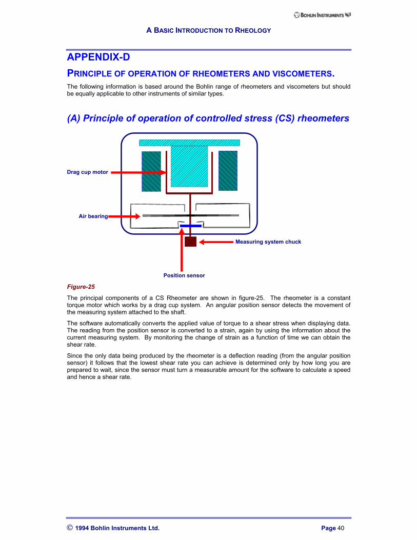
Appendix-D - Principle of operation of rheometers andviscometers.Principle of operation of controlled stress (CS) rheometers.

Principle of operation of controlled shear rate rheometers.

Index



SECTION 1 - INTRODUCTION TO RHEOLOGY

(A) Simple deformation under an applied constant force(Hookean response)To define the term STRAIN we will consider a cube of material with its base fixed to a surface (SeeFigure-1).

Figure-1

If we now apply a constant 'pushing' force, F, to the upper part of the cube, assuming the materialbehaves as an ideal solid, it will obey Hooke's law of elastic deformation and will deform to a newposition (Figure-2)

This type of deformation (lower fixed, upper moving) is defined as a SHEAR DEFORMATION.

Figure-2

The deformation δu and h are used to define the SHEAR STRAIN as :Shear Strain = δu/h

The shear strain is simply a ratio of two lengths and so has no units. It is important since it enables us toquote pre-defined deformations without having to specify sizes of sample, etc.

The SHEAR STRESS is defined as F/A (A is the area of the upper surface of the cube l x w) Since theunits of force are Newtons and the units of area are m2 it follows that the units of Shear Stress are N/m2

This is referred to as the PASCAL (i.e. 1 N/m2 = 1 Pascal) and is denoted by the symbol σ (in oldertextbooks you may see it denoted as τ).

For a purely elastic material Hooke's law states that the stress is proportional to the strain i.e.

Stress = G x Strain where G is defined as the SHEAR MODULUS (a constant)

Thus doubling the stress would double the strain i.e. the material is behaving with a LINEARRESPONSE. If the stress is removed, the strain returns instantaneously (assuming no inertia) to zeroi.e. the material has undergone a fully recoverable deformation and so NO FLOW HAS OCCURRED.



This Hookean behaviour is analogous to a mechanical spring which stretches when a weight issuspended from it (see Figure-3).

Figure-3

(B) Simple flow under an applied constant shear stress(Newtonian response)Let us again consider the case of the cube of material as described above but in this case assume thatthe material behaves as an ideal fluid. When we apply the shear stress (force) the material will deformas before but in this case the deformation will continually increase at a constant rate (Figure-4).

Figure-4

γ = δu x 1

h x S

The rate of change of strain is referred to as the SHEARSTRAIN RATE often abbreviated to SHEAR RATE and

is found by the rate of change of strain as a function of time i.e. the differential δ.SHEAR STRAIN / δ.TIME.

The Shear Rate obtained from an applied Shear Stress will be dependant upon the material’s resistanceto flow i.e. its VISCOSITY.

Since the flow resistance ≡ force / displacement it follows that ;

VISCOSITY = SHEAR STRESS / SHEAR RATE η = σ γ

The units of viscosity are Nm-2S and are known as Pascal Seconds (Pas).

If a material has a viscosity which is independent of shear stress, then it is referred to as an ideal orNEWTONIAN fluid. The mechanical analogue of a Newtonian fluid is a viscous dashpot which moves ata constant rate when a load is applied (see Figure-5).

Figure-5

Although the definitions covered so far are based on applying a shear stress and measuringthe resultant shear rate, the viscosity is simply the ratio of the one to the other, thus it follows that we willobtain the same answer for viscosity no matter which we apply and which we measure.

In theory therefore it does not matter if the instrument you are using (rheometer or viscometer) iscontrolled shear rate or controlled shear stress, you will still be able to measure the same flowcharacteristics. In practice however there are sometimes good reasons for using one type in preferenceto the other and a well equipped rheological laboratory should have access to both types of instrument.

Throughout this guide, I will try out show the good and bad points to both measurement techniques.



SUMMARY OF TERMS

Shear stress = Force / Area (NM-2 or Pascal, Pa) σShear strain = δu / h (Simple ratio and so No units)Shear rate = d.Shear strain / d.Time γViscosity = Shear stress / Shear rate η

(NM-2S or Pascal Second, Pas)

TYPICAL SHEAR RATE'S FOR SOME STANDARD PROCESSES

Process Typical range (S-1)

Spraying 104 - 105Rubbing 104 - 105Curtain coating 102 - 103Mixing 101 - 103Stirring 101 - 103Brushing 101 - 102Chewing 101 - 102Pumping 100 - 103Extruding 100 - 102Levelling 10-1 - 10-2Sagging 10-1 - 10-2Sedimentation 10-1 - 10-3

TYPICAL VISCOSITIES OF SOME COMMON MATERIALS [1]

Material Approximate Viscosity(Pas)

Air 10-5Acetone (C3H6O) 10-4Water (H2O) 10-3Olive Oil 10-1Glycerol (C3H8O3) 10+0Molten Polymers 10+3Bitumen 10+8



SECTION 2 - SELECTING MEASURING GEOMETRIESMeasuring geometries fall into three basic categories. These are:

(1) Cone and Plate(2) Parallel Plates(3) Cup and bob

Each type has its associated advantages and disadvantages which will be described in the followingsections.

(A) Cone and plate

Figure-6

This is in many instances the ideal measuring system. It is very easy to clean, requires relatively smallsample volumes and with a little care can be used on materials having a viscosity down to about tentimes that of water (10 mPas) or even lower.

Cone and plate measuring geometries are referred to by the diameter and the cone angle. For instancea CP4/40 is a 40mm diameter cone having an angle of 4°.

Often cones are truncated. These types of cone are positioned such that the theoretical (missing) tipwould touch the lower plate. By removing the tip of the cone, a more robust measuring geometry isproduced.

Since strain and shear rate are calculated using the angular displacement and the gap it follows that thesmaller the cone angle, the greater the error is likely to be in gap setting and hence your results. Byusing a relatively large angle (4°) it becomes easier to get reproducibility of gap setting. Unfortunately,the larger the cone angle the more the shear rate across the gap starts to vary!

In considering what cone angle to use it is worth looking at variations of shear against the gap comparedto reproducibility of gap setting. The following table of expected errors comes from work by Adams andLodge [2].

CONE ANGLE VARIATION OF SHEAR TYPICAL ERROR IN(O) RATE ACROSS GAP % CALCULATIONS %

1 0.03 0.022 0.21 0.083 0.28 0.184 0.49 0.325 0.77 0.507 1.5 0.9810 3.1 2.0

This shows that for a 4° cone the shear rate will vary by less than 0.5% across the gap giving data witharound 0.3% error. If a smaller cone angle is used, although the shear distribution error is small, theoperator to operator gap settings could easily introduce errors of over 5% even by experiencedoperators and so the larger angle gives a more acceptable error since it is a reproducible error.

When NOT to use a cone and plate.

Cone diameter

Cone angleTruncation



Because of the importance of correct positioning (often referred to as 'gap setting') a cone and plate isnot recommended when performing temperature sweeps unless your rheometer is fitted with anautomatic system for thermal expansion compensation.

If you must use a cone, use the largest cone angle and diameter available to you to minimise the errorsand try to set the gap at approximately the mid-range temperature of your sweep.

You should also avoid using a cone if the sample you are testing contains particulate material. If themean particle diameter is not some five to ten times smaller than the gap, the particles can 'jam' at thecone apex resulting in noisy data.

Materials with a high concentration of solids are also prone to being expelled from the gap under highshear rates, another reason to avoid the use of the cone.

(B) Parallel plate

Figure-7

The parallel plate (or plate-plate) system, like the cone and plate, is easy to clean and requires a smallsample volume. It also has the advantage of being able to take preformed sample discs which can beespecially useful when working with polymers. It is not as sensitive to gap setting, since it is used with aseparation between the plates measured in mm. (See Figure-7) Because of this it is ideally suited fortesting samples through temperature gradients.

The main disadvantage of parallel plates comes from the fact that the shear rate produced varies acrossthe sample. In most cases you will find that your software actually takes an average value for the shearrate.

Note also that the wider the gap, the more chance there is of forming a temperature gradient across thesample and so it is important to surround the measuring system and sample with some form of thermalcover or oven.

Parallel plate geometries are referred to by the diameter of the upper plate. For instance, a PP40 is a40mm diameter plate. The lower plate is either larger than or the same size as the upper plate.

When NOT to use parallel plates.When it is important to test samples at a known shear rate for critical comparisons the use of Parallelplates is not recommended.

Gap set height, h

Plate diameter



(C) Sample loading for cone and plate and parallel plate measuringgeometries.

Over filled

Figure-8

The sample should just fill the gap between the upper and lower elements. If the sample is likely toshrink during the test (due to solvent loss etc.) it is advisable to aim for a slight bulge as shown inFigure-8. If too much or too little sample is used, the torque produced will be incorrect leading to thedata being higher or lower respectively.

When using stiff materials with parallel plates, the best results can often be obtained by pre-forming thesample into a disc of the same diameter of the upper plate. The thickness should be very slightly thickerthan the required value so that the plates may be brought down such that they slightly compress thematerial, thus ensuring a good contact.

Some samples may be prone to skinning or drying. This will happen at the edge of the sample to itsexposure to atmosphere. To overcome this fit a solvent trap to the measuring system. Anothertechnique is to apply a fine layer of low viscosity (approximately 10 times thinner than the sample) siliconoil around the measuring systems. This works well provided that the oil and sample are not miscible andalso that relatively small rotational speeds are being used so as not to mix the oil into the sample.

(D) Cup and bob

Figure-9

Cup an bob type measuring systems come in various forms such as coaxial cylinder, double gap,Mooney cell etc (see Figure-9).

For DIN standard coaxial cylinders they are referred to by the diameter of the inner bob. i.e. a C25 is acoaxial cup and bob having a 25mm diameter bob. The diameter of the cup is in proportion to the bobsize as defined by the DIN Standard.

For double gap measuring systems they are usually referred to by the inner and outer diameters i.e. DG40/50.

Under filled

Correctly filled

DIN Coaxial cylinder

Double gapMooney cell



Cup and bob measuring geometries require relatively large sample volumes and are more difficult toclean. They usually have a large mass and large inertia's and so can produce problems when performinghigh frequency measurements (see ‘Viscoelastic Measurement’ section for more information).

Their advantage comes from being able to work with low viscosity materials and mobile suspensions.Their large surface area gives them a greater sensitivity and so they will produce good data at low shearrates and viscosities.

The double gap measuring system has the largest surface area and is therefore ideal for low viscosity /low shear rate tests. It should be noted that the inertia of some double gap systems may severely limitthe top working frequency in oscillatory testing (See later).

Some test materials may be prone to 'skinning' with time due to sample evaporation etc. To overcomethis fit a solvent trap onto the measuring system. Another technique is to float a very low viscosity (10 to100 times thinner viscosity) silicon oil on the top of the sample in the cup. This works well provided thatthe oil and sample are not miscible and also that relatively small rotational speeds are being used so asnot to mix the oil into the sample.

RULES OF THUMB FOR SHEAR RATE/ SHEAR STRESS; SELECTION.

Decrease cone/plate diameter to increase available shear stress.

Decrease bob surface area to increase shear stress

Decrease cone angle (or gap in a parallel plate) to increase availableshear rateRemember: smaller the angle the more difficult to set gap correctly)

Use large surface areas for low viscosity and small surface areas for highviscosities.

(E) Measurement of large shear rates on CS rheometersTo achieve very high shear rates on controlled stress rheometers can pose a few problems as describedbelow.

High shear rates on low viscosity materials using CS rheometers.The angular position / speed sensing system in controlled stress rheometers will have a maximum'tracking' rate before it is no longer able to measure the angular velocity correctly. If this velocity isexceeded the instrument will normally indicate some sort of over speed error.

If this happens at shear rates lower than you would like to obtain, change the measuring geometry toone with a smaller gap (a decrease in gap will increase the shear rate for the same angular velocity.)The highest shear rates can be obtained with a parallel plate with a very small gap or a tapered plugsystem.

High shear rates on high viscosity materials using CS rheometers.Since the shear rate = shear stress / viscosity it follows that to obtain a high shear rate with a highviscosity material you will need a high shear stress and so you may find that full stress will not producethe shear rate you require. Remember that small changes in the dimensions of the measuring systemswill make large changes to the available shear stress since the equations contain squared (coaxialcylinder) and cubed terms (cones and plates).

Example :

Maximum shear stress with a 1° 40mm cone = 596.8 Pa

Maximum shear stress with a 1° 20mm cone = 4775 Pa

i.e. halving the diameter increase the shear stress by a factor of eight.



(F) Summary of measuring geometry selectionThick materials can be tested with a cone and plate unless they contain particulate matter, in which caseuse a parallel plate. (remember that the shear rate will then only be an averaged value).

If you are performing a temperature sweep, use a parallel plate in preference to a cone and plate due tovariations in the gap with thermal expansion of the measuring system.

For low viscosity materials and mobile suspensions use a cup and bob type system. Maximumsensitivity is obtained with a double concentric cylinder (double gap).

For oscillatory measurements at high frequencies on low viscosity materials, the C25 cup and bob or aparallel plate with a small gap will produce the optimum test conditions.

For testing low viscosity materials when only small sample volumes are available, use a Mooney Cell(such as a 'small sample cell').

For all samples, if drying or skinning of the sample is likely to be a problem, use a solvent trap with themeasuring system or alternatively use a low viscosity silicon oil as a barrier if it is not likely to alter thesamples properties.



SECTION 3 - FLOW CHARACTERISATION

(A) The viscometry testThere are generally two types of simple flow characterisation tests for viscometry . These are Steppedshear stress / shear rate or Ramped shear stress / shear rate.

The types available on your particular instrument will depend upon the configuration of your rheometersoftware.

Stepped shear.Individual shear values are selected. Each shear is applied for a user set time and the shear rate, shearstress and viscosity are recorded for each value.

The individual points are then either joined up 'dot to dot' fashion or using a rheological model toproduce the flow curve and the viscosity curve.

This test method is the generally the preferred way of generating flow and viscosity curves.

Ramped shearThis test applies a continuously increasing or decreasing shear (in a ramp) throughout the complete test.Measurements are taken at user defined intervals along this shear gradient.

The three main uses of this technique are:

1 To perform rapid 'loop' tests of viscosity for use in QC type environments.

2 To simulate processes where the shear changes in a ramped fashion (e.g. start up of a roller,chewing etc..)

3 To determine some point where the material starts to flow (the yield point) although this isnormally only done on controlled stress rheometers.

(B) Flow curvesThe measured viscosity of a fluid can be seen to behave in one of four ways when sheared, namely :

1 Viscosity remains constant no matter what the shear rate (Newtonian behaviour)

2 Viscosity decreases as shear rate is increased (Shear thinning behaviour)

3 Viscosity increases as shear rate is increased (Shear thickening behaviour)

4 Viscosity appears to be infinite until a certain shear stress is achieved (Bingham plastic)

Over a sufficiently wide range of shears it is often found that the material has a more complexcharacteristic made up of several of the above flow patterns.

Since it is the relationship of shear stress to shear rate that are strictly related to flow we can directlyshow the flow characteristics of a material by plotting shear stress v shear rate. A graph of this type iscalled a Flow Curve.

The graphs in Figure-10 show the flow curves and viscosity curves of the four basic flow patterns.



0.2

0.5

1

2

5

0

2

4

6

8

10

12

0 2 4 6 8 10

Shear rate -->

Shear stress mPa

Newtonian

Viscosity

0

50

100

150

200

250

0

10

20

30

40

50

60

0 5 10 15

Shear rate

Shear stress

Shear thinning

Viscosity

0

50

100

150

200

250

0

10

20

30

40

50

60

0 5 10 15

Shear rate

Shear stress

Shear thickening

Viscosity

0

50

100

150

200

250

0

10

20

30

40

50

60

0 5 10 15

Shear rate

Shear stress

Bingham Plastic

Viscosity

Figure-10

The exact behaviour of materials can often be described by some form of rheological model. Some ofthe more commonly used models are described in the following section.

Models for fundamental flow behaviourThese models describe the simple flow behaviour as shown in the previous graphs. Most materials willstart to deviate from these relationships over a sufficiently large shear range. They are well suited tostudying materials over a small shear range or where only a simple relationship is required.

NewtonianThis is the simplest type of flow where the materials viscosity is constant and independent of the shearrate. Newtonian liquids are so called because they follow the law of viscosity as defined by Sir IsaacNewton:

σ = γ * η

Shear Stress = Shear rate * viscosity

Water, Oils and dilute polymer solutions are some examples of Newtonian materials.

Power law - (or Ostwald model)Many non-Newtonian materials undergo a simple increase or decrease in viscosity as the shear rate isincreased. If the viscosity decreases as the shear rate is increased the material is said to be ShearThinning or Pseudo plastic. The opposite effect is known as shear thickening. Often this thickening isassociated with an increase in sample volume; this is called ‘dilatency’.

The power law is good for describing a materials flow under a small range of shear rates. Most materialswill deviate from this simple relationship over a sufficiently wide shear rate range.

σ = η * γn

Shear stress = viscosity * Shear rate n

Where 'n' is often referred to the power law index of the material.



If n is less than one, the material is shear thinning, if n is more than one then material is shearthickening. Polymer solutions, melts and some solvent based coatings show Power law behaviour overlimited shear rates.

BinghamSome materials exhibit an 'infinite' viscosity until a sufficiently high stress is applied to initiate flow.Above this stress the material then shows simple Newtonian flow. The Bingham model covers thesematerials:

Shear Stress = Limiting shear Stress + viscosity*shear rate

The limiting stress value is often referred to as the Bingham Yield Stress or simply the Yield Stress ofthe material. It should be noted that there are many definitions of Yield stress. For further information onthis topic see the section on Yield values later.

Many concentrated suspensions and colloidal systems show Bingham behaviour.

Herschel BulkleyThis model incorporates the elements of the three previous models

Shear stress = limiting stress + viscosity * shear raten

Special Cases of the model:A pure Newtonian material has limiting stress=0 and n=1A power law fluid has limiting stress=0 and n=power law indexA Bingham fluid has limiting stress= 'Yield value' and n=1

This model many 'industrial' fluids and so is often used in specifying conditions in the design of processplants.

VocadloThis is similar to Herschel Bulkley although it will some times prove a better representation of the fluid.



Models for more complex flow behaviourThese relationships have been developed as 'enhancements' to the fundamental models. They tend togive a more realistic prediction of flow over a wider range of conditions.

EllisThis describes materials with power law behaviour at high shear rates but Newtonian behaviour at lowshear rates.

Shear rate = K1* shear stress + K2*shear stress^n

Where K1 and K2 are simple constants and n is material index.

This model is often used to describe polymeric systems as it generally gives a better representation thanthe power law model.

CassonThis model is used for materials that tend to Newtonian flow only at stresses much higher than thematerials Yield stress.

shear stress^0.5 = Yield stress^0.5 + K*shear rate^0.5

This model is often used for suspensions. It is also used by some confectionery manufactures todescribe the properties of molten chocolate.

MooreThis model is capable of predicting flow properties over a wide range of shear rates since it incorporatesterms for both limiting low shear rate and high shear rate viscosities.

CrossThis is an extension of the Moore model but with containing four independent parameters (Moore hasthree) It is often able to accurately describe the shear thinning behaviour of disperse systems.

SiskoThis describes a material with a limiting high shear rate viscosity. Although the limiting low shear rateviscosity is infinite, the model does not in general describe a material with Yield.

Viscosity = high shear viscosity + k*(1/shear rate)^m

Note : if m=1 then this equation is the same as the Bingham.



(C) Yield valuesIf we think back to our basic definitions (section 1) we recall that when the applied shear stress isremoved after a deformation has occurred, the strain should return to zero. If it does not eventuallyreturn to zero, we say that flow has occurred.

The yield stress of a material is usually defined as the maximum stress below which no flow will occur.However the accurate measurement of this point requires the determination of whether the strain hasreached a value of zero. It is generally believed that if you wait long enough and can measure sufficientlysmall strains, you will find that no materials have a true yield stress.

In practical terms however the yield stress (or yield point) is defined in terms of whether the material hasundergone a degree of deformation that is significant to the size and time scales of a particular process.Thus yield becomes dependant upon not only the stress but also the measured strain and the elapsedtime.

There are three commonly used methods for determining yield, each of which has its own advantagesand disadvantages. These are as follows:

Flow curve methodUse the Flow Curve for the material and extrapolate back to where the shear rate = zero to find theshear stress value. The disadvantage of this method is that you are not measuring the value butcalculating it by assuming the material follows simple Newtonian behaviour immediately after it yields i.e.Bingham flow. For controlled shear rate instruments this is the only method that can be used.

Step stress testThis consists of applying a small stress, holding for a pre-defined time and measuring the strainresponse. The stress is gradually stepped up until a measurable 'flow' is obtained. This method isprobably the most accurate way of characterising the yield point of a material but it can be a very timeconsuming process. As this test is essentially a multiple creep test, it will be covered more fully insection-4.

Ramp stress testThis involves applying a gradually increasing stress and monitoring the instantaneous viscosity for aninflexion of the curve i.e. the onset of flow. By altering the ramp rate, time effects can be taken intoconsideration. This method is used by the Bohlin Yield Stress test and will be explained in greater detaillater.



(D) Time and temperature dependenceAs well as looking at the rheological characteristics of a material as a function of shear, two otherfactors, namely time and temperature dependence must be looked at as well.

Temperature dependenceThe viscosity of a material is usually found to decrease with an increase in temperature, assuming nophysical/chemical changes are being induced by the applied heat energy. The temperature dependencecan be determined by running a temperature gradient programme. Samples usually have some degreeof heat capacity, known informally as 'thermal inertia' i.e. if the surrounding temperature is altered thenthey will take time to change their overall temperature. This is an important point to consider whenselecting the rheometer's temperature ramp rate. To find a measure of this lag, manually increase ordecrease the temperature and monitor the time it takes for the sample viscosity to change.

Note that you will also need to be certain that the sample does not exhibit any significant time dependantproperties throughout the time scale of the test.

It is important to establish the temperature dependence of your sample if you wish to state degrees ofaccuracy for your measurements. As an example consider the viscosity of water which alters by some3% per °C. To maintain a ± 1% accuracy in the measurements you must hold the temperature to ±0.3°C.

Arrhenius modelThe viscosity of Newtonian liquids decreases with an increase in temperature approximately in line withthe Arrhenius relationship.

This model describes a materials variation in viscosity with ABSOLUTE temperature.

Viscosity = c * e (k/temperature in Kelvin)

(k is related to the flow activation energy E and Boltzmann's constant R by k=E/R).

Time dependenceSome materials have flow characteristics that are dependant on the 'shear history' of a material. A wellknown example of this is tomato ketchup. When left long enough, the inter-particle interaction causesthe ketchup to 'stiffen' up, seen as an increase in viscosity. To get the sauce to flow out you have toshake the bottle (i.e. shear it) This destroys the samples structure and the viscosity decreases.

A reversible decrease of viscosity with time under steady shear is referred to as thixotropy (if the sheargives a temporary increase in viscosity, it is termed negative thixotropy, sometimes referred to asrheopexy although this is not the preferred term).

If the act of shearing a material produces a non-recoverable change in the viscosity it is referred to asrheodestruction (or rheomalaxis). Again, theoreticians argue that there is no such thing asrheodestruction but that the time required for complete rebuild is just very long and so does not appearto happen.

It should be noted that these changes are purely time related and the materials flow characteristic needto be studied as well. It is possible that a material could be, say, both thixotropic and shear thickening.

When materials have time dependence it is important to take steps to pre-condition them such that flowcurves can be compared with a common shear history. The best method to do this is to put the sampleinto the rheometer and subject it to a high shear rate for a time sufficient to destroy any structure, (this iswhy it is not a good idea to use a syringe to apply the sample if you wish to measure the structure of thematerial since you will produce very high shear rates and could destroy the samples structure) then allowit to rest for a fixed time to recover again before taking any measurements.

You will need to study the time dependence of the material in order to design a conditioning regimesince the changes can happen over time scales of a few seconds to many hours or even days. Inaddition, the rate of change of viscosity may also be affected by the sample temperature!

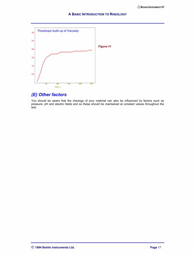
Figure-11 shows the rebuild in viscosity of a material after pre-shear. After approximately 100 secondsmost of the recovery has occurred. Thus you could design a test that pre-sheared the sample, waitedfor two minutes and then performed the rest of the test. This way all materials should be starting fromthe same reference point.



Figure-11

(E) Other factorsYou should be aware that the rheology of your material can also be influenced by factors such aspressure, pH and electric fields and so these should be maintained at constant values throughout thetest.

0.5

1.0

1.5

2.0

2.5

3.0

50 100 150 200 250

Time -->

Thixotropic build up of Viscosity



(F) Equilibrium flow curvesWe stated earlier in this chapter that the viscometry test could produce either a ramp or a stepped flowcurve . It is important to be aware of the differences between these two.

If we look at the case of a controlled stress rheometer, we see that we impose a constant force i.e.stress and measure the resultant deformation as a function of time. If the material is a pure Newtonianliquid we will obtain a linearly changing deformation i.e. simple Newtonian flow. For all other materialsthe effect will not be as simple. If the applied stress is relatively small, it may be fighting against thematerials 'structural' properties i.e. elastic elements, time dependant changes etc.

The response of the material will follow something along the following lines ;

ELASTIC DEFORMATIONVISCOUS FLOW ON TOP OF ELASTIC DEFORMATION

PURE VISCOUS FLOW

If the material is a pure solid, we will either obtain a fixed but fully recoverable deformation (i.e. below thematerials yield point) or a rapid fracture if we are above it. Since in rheology we are only interested inlooking at fluids it follows that there will also be some viscous elements in the material and these willwork to resist the applied stress and hence the 'fracture' of the elastic component will be delayed a smallinstant.

Depending on the strength of the viscous and elastic elements and the value of the applied stress, it ispossible that we may need to wait a considerable length of time until we have deformed the materialsufficiently to remove all elastic deformation and are just measuring the pure viscous flow. Even incontrolled shear rate instrumentation the delay may be of a noticeable interval.

In stress viscometry tests the software monitors how 'compliant' the material is as a function of time. Thecompliance of a material is simply defined as the STRESS APPLIED / STRAIN PRODUCED and as wehave seen should be a linear function as a function of time for pure viscous flow (Figure-12).

When this state is achieved it will be found that the measured shear rate is constant and the slope of thecompliance curve as a function of time is constant ie. the differential gives a value of 1.00. This is thenumber shown by the Bohlin software.

Figure-12

Under these conditions we know that we can measure the viscosity of the material without it containingany effects due to elasticity. This is very important since many processes are shear rate controlled andcan be thought of as being able to apply up to an infinite torque if required to obtain the specified shearrate. In controlled shear rate rheometers the time to reach equilibrium is generally small and so thenormal delay interval is sufficient.

Thus, the stepped shear test allows us to wait for this equilibrium condition at each applied valuewhereas the ramped test does not. There are occasions however where the use of a ramp is preferredto the use of step. This is covered in the next section.

Time --->

Approach to pure viscous flow

Slope = 1 --->

Shear rate Compliance



(G) Ramp viscometry testsIn ramp testing, if the shear range is sufficiently large and the ramp rate fast enough, the materials non-flow structure will be largely destroyed before any measurements are taken and so a simple flow curvecan be produced. This method is fine for quick QC type applications although you should be aware thatit may not give absolute readings of viscosity since no check is made that you are only recording steadyflow conditions. If you change the test conditions (e.g. the ramp rate of the shear range) the dataproduced can not be directly compared to results generated by the previous test conditions.

Many people use this test to measure a materials time dependant properties (i.e. thixotropy) bysweeping up and then down in shear and measuring the area of the looped flow curve (known as thehysteresis loop). Again, although this is fine for a simple QC test, you should be aware that changingany of the test parameters will invalidate comparisons with previously generated data. For measurementof thixotropy / structure rebuild you are best to perform a pre-shear followed by a single frequency ormultiwave oscillation test (please refer to the section on oscillatory testing for more information).

Yield stress measurements on a controlled stress rheometerSuppose we limit the ramp to small stresses and put a longer sweep time (say the minimum stressavailable, up to 1 Pa over 120 seconds) then we will be able to see the effect of the elastic elements asan increase in the 'instantaneous' viscosity since this value is calculated assuming that the relationshipViscosity = Stress / Shear rate holds, which it will not do until we break into pure viscous flow. As thematerial starts to flow, the instantaneous viscosity will be seen to change rapidly from an increasingvalue to a decreasing value and the stress being applied at this instant is recorded as the Yield Stress(see Figure-13).

Figure-13

0

5

10

15

20

25

30

35

0.001 0.01 0.1 1

Shear rate 1/s

Viscous flowElastic deformationon viscous flow

Bohlin Yield Stress Test



DESIGNING YOUR OWN FLOW CHARACTERISATION TESTSThe above section has now hopefully given an insight into the many type of flow characteristic that canbe expected from a material. All of these points must be borne in mind if you are to design tests thatproduce valid and useful data.

Questions to ask when designing a test protocol.The following 4 points should always be considered when designing your tests :

(1) WHY !

Perhaps the most important question to be asked is why do you want to characterise the material. Forexample, is it for use on the factory floor for QC or is it to enable the design of a new formulation?

Once this is established the range of variables and conditions can often be radically reduced. Also theprotocol can be designed to give the required balance between precision, speed and reproducibility.

For instance, if you know what shear rates or shear stresses you require, pick a measuring system andmeasurement head capable of generating and recording the data.

(2) WHAT ARE YOU TRYING TO DETERMINE ?

Do you wish to simply measure a viscosity value at a certain shear rate ? Do you wish to study ageingcharacteristics or dependence upon temperature ? Are you trying to obtain as full a characterisation ofthe material as possible for use on comparative purposes either for QC or in developing newformulations / better products?

(3) DOES MATERIAL HAVE TIME / TEMPERATURE DEPENDENCY?

If this is suspected or not known it should be determined first. There is no point trying to measure amaterial if the time taken for the test allows a significant change in the material to take place. Someform of preconditioning will be required if you are trying to obtain comparative data. This could consist ofchanging the samples temperature for a fixed time or pre-shearing the material.

An important consideration is the temperature of a material before it is placed into the rheometer. If it islikely to vary widely use a long equilibrium time to ensure that the material has sufficient time to reachtest temperature.

(4) WHAT TYPE OF MEASUREMENT SYSTEM IS BEST ?

The selection of measuring geometry is relatively straightforward if you consider the following points:

What shear rates / stresses / viscosities are you working with ? Use the data sheets and the informationcontained previously in the course to obtain the required combination.

What is the material like ? Is it 'pourable' or highly viscous ? Is it a gel or a suspension ? Does itcontain particulate material ? Does it have a solvent base ?

The previous section on measuring system selection covers the selection on the above points.



PITFALLSWhen you produce data on any computer controlled instrument, you should be aware that sometimesthere are errors arising from the conditions you have selected. The software can not always point theseout to you. The following section lists some of the more common rheological problems that may occur.

Turbulent or secondary flowFor rotational rheometers and viscometers it is assumed that at all times the flow of the fluid in themeasuring systems is steady, or laminar and one dimensional. That is, no variation with time exists andthe fluid moves only in the direction of rotation (see Figure-14).

Figure-14

In general, for narrow gaps and modest rotational speeds, this type of flow is attained and satisfactoryviscosity data may be recorded. However, as the rotational speed is increased, a transition from asteady one dimensional flow pattern to a more complex but steady three dimensional flow takes place.This flow pattern takes the form of vortices whose axes lie in the circumferential direction (see Figure-15).

This type of flow was first described by Taylor (1936) and is termed TAYLOR VORTEX FLOW.

Figure-15

In most cases the onset of this SECONDARY flow will be seen as a sharp and distinct increase in thetorque required to obtain a given shear rate. The consequence of this is an apparently rapid increase inthe recorded viscosity.

At even higher speeds the flow becomes turbulent but in viscometry we are primarily interested inensuring we remain below the threshold at which the development of Taylor vortex flow takes place.

When the inner cylinder rotates, the fluid at the inside of the measuring system is moving rapidly andtends to move outwards under centrifugal action. This must be replaced by fluid from elsewhere and soa recirculating vortex flow structure develops. Simplistically, this is the mechanism responsible for theonset of secondary or ‘Taylor Vortex’ flow.

Secondary flow problems are largely restricted to tests using coaxial cylinders since cone and plates aregenerally used with more viscous samples.

As an example we will consider the flow curve for water measured on a controlled stress rheometerusing a large double gap concentric cylinder.

Laminar Flow

Taylor Vortex Flow



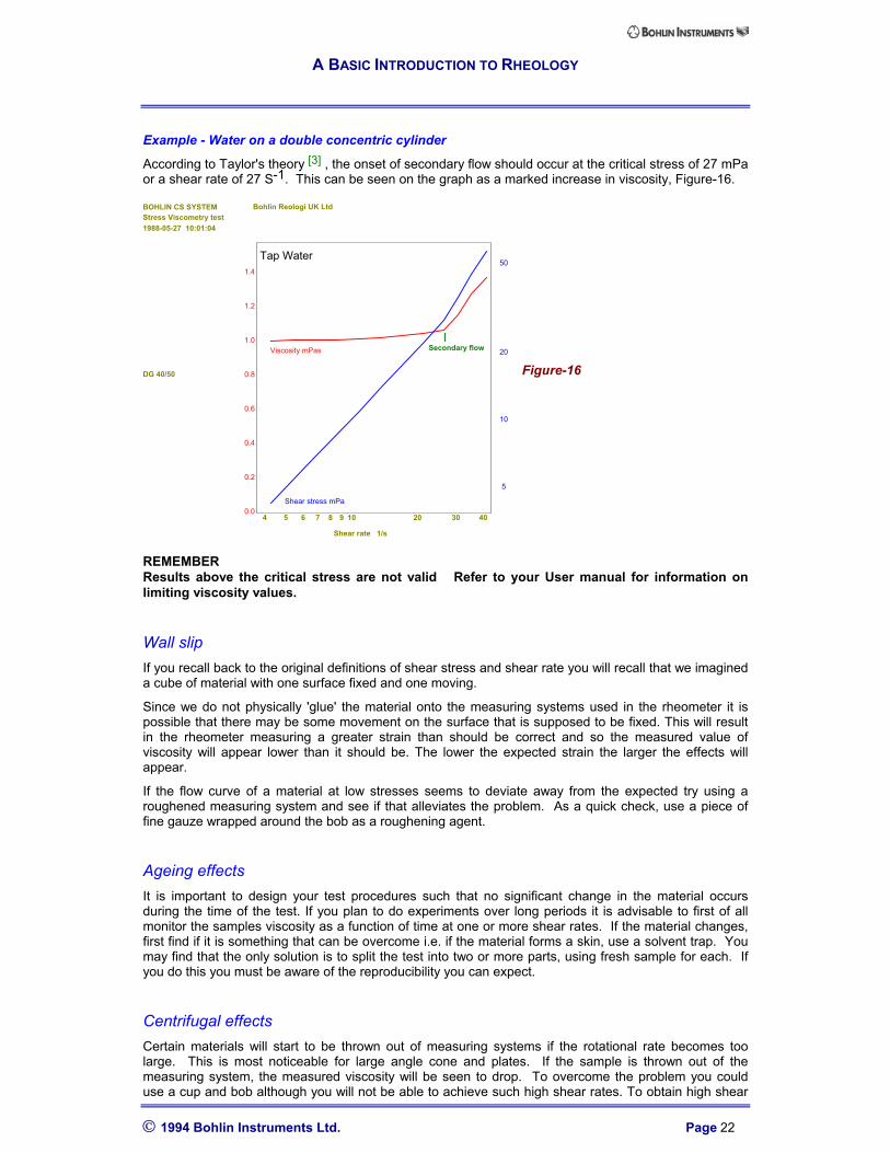
Example - Water on a double concentric cylinder

According to Taylor's theory [3] , the onset of secondary flow should occur at the critical stress of 27 mPaor a shear rate of 27 S-1. This can be seen on the graph as a marked increase in viscosity, Figure-16.

Figure-16

REMEMBERResults above the critical stress are not valid Refer to your User manual for information onlimiting viscosity values.

Wall slipIf you recall back to the original definitions of shear stress and shear rate you will recall that we imagineda cube of material with one surface fixed and one moving.

Since we do not physically 'glue' the material onto the measuring systems used in the rheometer it ispossible that there may be some movement on the surface that is supposed to be fixed. This will resultin the rheometer measuring a greater strain than should be correct and so the measured value ofviscosity will appear lower than it should be. The lower the expected strain the larger the effects willappear.

If the flow curve of a material at low stresses seems to deviate away from the expected try using aroughened measuring system and see if that alleviates the problem. As a quick check, use a piece offine gauze wrapped around the bob as a roughening agent.

Ageing effectsIt is important to design your test procedures such that no significant change in the material occursduring the time of the test. If you plan to do experiments over long periods it is advisable to first of allmonitor the samples viscosity as a function of time at one or more shear rates. If the material changes,first find if it is something that can be overcome i.e. if the material forms a skin, use a solvent trap. Youmay find that the only solution is to split the test into two or more parts, using fresh sample for each. Ifyou do this you must be aware of the reproducibility you can expect.

Centrifugal effectsCertain materials will start to be thrown out of measuring systems if the rotational rate becomes toolarge. This is most noticeable for large angle cone and plates. If the sample is thrown out of themeasuring system, the measured viscosity will be seen to drop. To overcome the problem you coulduse a cup and bob although you will not be able to achieve such high shear rates. To obtain high shear

0.0

0.2

0.4

0.6

0.8

1.0

1.2

1.4

5

10

20

50

4 5 6 7 8 9 10 20 30 40

Shear rate 1/s

Viscosity mPas

Shear stress mPa

BOHLIN CS SYSTEM Bohlin Reologi UK LtdStress Viscometry test1988-05-27 10:01:04

DG 40/50

Tap Water

Secondary flow



rates with least risk of sample expulsion use a small angle cone or a parallel plate with a small gap or atapered plug measuring system.

Remember that you may start to generate noisy data when running particulates with small gaps sincethe particles may jam into each other (a rough rule of thumb often used to ensure good data is to use agap at least 10 times larger than the mean particle size).

Measurement of small shear rates on controlled stress rheometersThe angular position sensor on the Bohlin CS is a digital based system, that is it produces discreet stepsfor angular movement and is thus limited to the smallest angular position it can measure. If you wish tomeasure very small shear rates you must therefore be prepared to wait such that a large enough angulardeflection is obtained to give you good data. Make sure also that you have optimised on the measuringsystem best suited to give you low shear rates.



SECTION 4 CREEP ANALYSISMost materials are formed by a combination of viscous and elastic components. If a sufficiently largestrain is applied it is possible to break the 'structure' of the material i.e. the elastic part, resulting in purelyviscous flow. This is the principle of the viscometry tests that we have looked at so far.

At low strains however, the elastic component will play a major part in contributing to the materialsbehaviour and so it is important to be able to measure and characterise it.

One method available to us on controlled stress rheometers is the creep test. (a similar test, stressgrowth, is available on controlled shear rate instruments. See later for more information on this test.)

Creep is defined as 'the slow deformation of a material, usually measured under a constant stress'. If weapply a small stress to a viscoelastic material and hold it constant for a long period of time whilstmeasuring the resultant strain we will see behaviour initially from elastic components followed shortly byviscoelastic effects. At sufficiently long time scales we will obtain effects only from the viscouscomponents since the resultant strain is large enough to have 'used up' the elastic component (seeFigure-17). If we refer back to the section on equilibrium flow curves you will remember that we onlyrecorded data in this later stage when we knew that what we were measuring was pure viscous flow.The creep test records the information from the moment we apply the stress and hence gives a measureof elastic, viscoelastic and viscous components.

By applying small stresses it is also possible to mimic gravitational effects on a sample to assist inpredicting effects such as sedimentation, sagging and levelling. The shear rates produced under theseconditions will typically be of the order 10-5 - 10-6 S-1.

(A) Principle of operationIn a creep test a user selected shear stress is 'instantaneously' applied to a sample and the resultantstrain monitored as a function of time. After some predetermined time the stress is removed and thestrain is again monitored. The three typical response curves are shown in figure-17

Time --> Time --> Time -->

Stress on Stress off Stress on Stress off Stress on Stress off

γ γ γ

PURE ELASTIC PURE VISCOUS VISCOELASTICFigure-17

The third case shows a typical curve produced by a viscoelastic material. The actual shape will bedetermined by the interaction of the viscous and elastic components.

Since the actual change of strain will be dependant upon the applied stress, it is usual to talk about thecompliance rather than the strain. The compliance is defined simply as the ratio of the strain to theapplied stress and is denoted by the letter J (J=strain/stress). By using this notation, creep curves maybe directly compared even if they were not measured under the same applied stress.

(B) Time scales and the Deborah NumberTo fully recognise the concept of creep, time factors must be understood with respect to mechanicalbehaviour of the samples. Rapid response times (often fractions of a second) are mainly indicative ofelastic phenomenon whereas viscous phenomenon usually take seconds or even minutes to occur. Thecorrect experiment time is important to enable fast and slow phenomenon to be accurately resolved. Toenable us to put numbers to a materials response characteristics we use a function called the Deborahnumber.



The Deborah NumberTo understand whether a material will tend to behave more as a fluid or more as a liquid two factorsmust be looked at. These are the time scale of the process/experiment, T and the characteristicrelaxation time of the system, τ.

The Deborah number is defined as De = τ / T

De < 1 liquid like behaviour De = 1 viscoelastic behaviour De > 1 solid like behaviour

The time τ is infinite for a Hookean elastic solid and zero for a Newtonian viscous liquid and is actuallythe time taken for an applied stress (or strain) to decay to 2/3 its initial value. (The decay is exponential.)The relaxation time can be found by performing a frequency sweep on the sample and taking τ = 1/ωxwhere ωx is the angular velocity (2 *π * frequency) within the linear region at the point where G'=G" orby use of the relaxation test. (see later)

The above can be summarised simplisticaly by saying 'everything flows if you wait long enough' (thename Deborah comes from an Old Testament prophetess who told of "mountains flowing before theLord" !)

It can be seen therefore that a sample may show solid-like behaviour either because it has a relativelylong characteristic relaxation time or it is being subjected to a process of time scales considerablyshorter than the materials characteristic relaxation time. The creep test takes the sample through shorttime scale response to long time scale response. This can be seen in the example creep curve inFigure-18.

Figure-18

Data at the very start of the test relates primarily to a pure elastic deformation and is referred to as the'instantaneous' or 'glassy' compliance. At longer time scales the deformation will be due to both viscousand elastic elements and is referred to as damped or delayed elastic compliance. At sufficiently largeenough time scales the resultant deformation will be purely due to viscous flow. When the material is inpure viscous flow the differential of the slope of the curve will be 1.00. The Bohlin software gives areadout of the slope as the test progresses and can be made to automatically accept the data when this'steady state' is attained. This is presented as dLn.j/dLn.t (i.e. the change in compliance as a function oftime) in the software.

Zero shear viscosityAfter sufficiently long time scales where the steady viscous flow is achieved, the samples viscosity canbe estimated from the slope of the compliance curve.

At sufficiently low shear rates it is found that most materials either have a viscosity that tends to infinity(yield stress) or have a viscosity that becomes independent of shear rate (the low shear Newtonianplateau). To verify the materials behaviour you would run a creep test to obtain the low shear viscosity,then repeat the creep test but with a lower shear stress (hence producing a lower shear rate) If the twotests produce the same reading of viscosity then you have found the materials zero shear viscosity. Ifyou keep decreasing the stress and the viscosity keeps increasing, it is possible that the material has ameasurable yield stress (see next section).

A materials zero shear viscosity is useful in predicting such factors as storage stability, levelling etc.Equations for these are given in Appendix-B.

2

5

10

2

5

10

5 10 15 20 25 30

Time s

J m1/Pa Jr m1/Pa

BOHLIN CS SYSTEM Bohlin Reologi UK Ltd. Applications Lab.Creep & Recovery test

V 2.89E+03Stress 1.00E+02

Joc 5.08E-03Jor 4.91E-03

T 25.0 - 25.0 C

Creep Curve

Recovery curve

Joc

Jor



Measurement of yield stress by 'stepped creep' testsBy repeating creep tests at lower and lower shear stress values you can determine the yield stress of amaterial quite accurately.

In the ramped stress viscometry test mentioned previously, we gradually ramp up the stress anddetermine the point that the structure breaks down or 'ruptures' Since the yield point of a material isdependent not only upon the applied stress but also the time the stress is applied for, a much moreaccurate way of determining yield would be to hold a stress for a pre-set period of time, then step up to aslightly higher stress and hold, continuing this process until the material started flowing. In a creep test,if we apply a stress below the materials yield value, we find that the sample will deform due toviscoelastic properties, but will not start to flow. This will be seen as the compliance curve tending tolevel off to a horizontal curve (slope -> 0) Therefore we can determine if the material is likely to flow byseeing if the slope of the curve (dLn.J/dLn.t) is increasing towards unity (tending to flow) or decreasingtowards zero (no flow).

NOTE: Since this technique can be lengthy you will need to determine that the material does not havesignificant time dependant properties over the observation time of this test.

It is important that we let the sample recover after applying each stress i.e apply stress for 30 seconds,remove stress and rest for 30 seconds, then repeat at a higher stress and so on.

The ramped viscometry test is a good method of determining the yield stress and of course is very rapid.The method of stepped stresses is more accurate and therefore may produce significantly differentanswers from the other test. It is a good idea to try both techniques and see which best suits yourmaterials and requirements.

Measurement of elasticityThe creep test provides a method of determining the amount of elasticity in a sample. This value isdenoted as Jo and is calculated by extrapolating back along the creep curve when in steady viscousflow. The intercept is then a measure of Jo and since it is obtained from the creep test it is recorded asJoc. This method is fine for estimating Jo but it is prone to error since it generally involves extrapolatingback from a large number to obtain a small number. A far better method of obtaining Jo would be tomeasure it directly and this is done by the Creep Recovery test.

When we have obtained a state of steady viscous flow, if we remove the stress and wait for at least aslong as it took us to obtain viscous flow, the material will recoil due only to the elasticity. By measuringthis recoil, or recoverable compliance, we obtain a value for Jo denoted in the software as Jor. Generallyyou will find that Joc and Jor have the same order of magnitude but that Jor is more accurate.

When to do creep recovery tests.If the value of J becomes quite large during the creep test, it is more likely that Joc will not be asaccurate as could be obtained by performing a creep recovery test. The disadvantage of doing the fullcreep followed by creep recovery is that you must run the recovery part for at least as long as the creeppart to guarantee that all of the elasticity has been recovered (since the viscous part produces viscousdamping). This effectively doubles the time required and could cause problems if the material is likely tochange due to drying, skin formation etc. The accuracy of Joc should thus be looked at in relationship tothe reliability of obtaining good Jor data.



SECTION 5 - VISCOELASTIC CHARACTERISATIONFlow characterisation tests do just that, i.e. tell you how a material is likely to flow under an imposedconstant shear rate or shear stress. They tell only about the materials VISCOUS properties (resistanceto flow).

To measure a materials viscoelastic properties we can use creep testing (as described in the previoussection) or alternatively we can use oscillatory techniques. The technique used is to apply a stress orstrain whose value is changing continuously according to a sine wave equation. Thus the inducedresponse (strain or stress) will also follow a sine wave.

Thus it can be seen that we can continuously excite the sample but never exceed a certain strain andhence we do not destroy the sample structure. (providing steps are taken to keep the strain smallenough).

If we 'over strain' the sample, we will start to destroy the elastic structure of the material and so it isimportant to keep the strain low. The technique used by the software in controlled stress instruments isto continuously adjust the applied stress so that the resultant strain is held at a specified value.

If you remember back to section 1 we talked about Hookean deformation (analogous to a spring beingextended) and Newtonian flow (analogous to a viscous dashpot) most materials are made up of acombination of these two properties. Hooke's law is a simple linear relationship, that is if you double theapplied stress you double the measured strain. Provided the strain produced is small enough it is saidthat you are working in the materials REGION OF LINEAR STRAIN RESPONSE or more simplyLINEAR REGION.

The calculations used in the software are only valid in this linear response region.

Thus, before performing oscillation tests on a material you must verify that the test conditions fall intothis regime. This is easily tested by oscillating at a fixed frequency and slowly increasing the appliedamplitude (strain or stress). The measured values for the viscoelasticity will remain constant. When theapplied stress becomes too great, the induced strain will start to cause the material to 'rupture' i.e. youwill obtain some flow on top of the deformation. This will be seen as the measured value of elasticityfalling whilst the measured viscous component will start to increase. Provided you work at strains belowthis point you will be working in the materials linear region. If it is difficult to find the linear region,increase the cone angle or the parallel plate gap to produce lower strains in oscillation.

(A) Definition of elastic and viscous componentsAs stated earlier, if we apply a sinusoidally varying stress to a sample, we will induce a sinusoidallyvarying strain (and vice versa for applied strain) response. If we think back to how the stress effects thesample for a pure solid and a pure liquid you will remember the following :

For a Hookean Solid :Shear Stress = Shear Strain x G (a constant)

For a Newtonian liquid :Shear Stress = Shear Strain rate x Viscosity (a constant)

So for a pure solid the strain is controlled by the absolute value of shear stress, whereas for a liquid it isthe rate of change of strain that is controlled by the stress

If we consider one complete cycle of the sine wave as 360° then we can talk about differences of phasebetween the two waves as PHASE ANGLES.

In the case of a pure solid, since the strain is directly related to the stress, it will be at a maximum whenthe stress is a maximum and zero when the stress is zero. The strain response is said to be totally INPHASE with the applied stress i.e. the PHASE ANGLE = 0° (see Figure-19).

If the material is a pure viscous liquid we find that it will be the strain rate that is exactly following thestress. If you look at the graph of strain rate as a function of time you can see that the strain alternatesbetween a positive and negative extreme accelerating and decelerating between these two values.

Therefore, when the strain rate is at a maximum the rate of change of strain will be zero, likewise whenthe strain is zero, the rate of change will be a maximum. The resultant strain will therefore be totally (90°)out of phase to the applied stress (see Figure-20).



Figure-19

Figure-20

In practice, most materials are a combination of viscous and elastic components and so the measuredphase angle will be somewhere between 0° and 90°. The closer to 90° the more fluid like the behaviourof the material under test.

Modulus ValuesWe stated earlier that Hooke's law relates the strain to the stress via a material constant known as theMODULUS, G. (G = stress / strain)

In the oscillation test the stress and strain are constantly changing but we can consider any number of'instantaneous' values to obtain a value of 'viscoelastic G'. This is referred to as the materialsCOMPLEX MODULUS, G* and is obtained from the ratio of the stress amplitude to the strain amplitude.This modulus is the 'sum' of the elastic component (referred to as G' often called the STORAGEMODULUS to signify elastic storage of energy since the strain is recoverable in an elastic solid), and theviscous component (referred to as G'' often called the LOSS MODULUS to describe viscous dissipation[loss] of energy through permanent deformation in flow).

We define the complex modulus as:

G* = G' + i x G''

By measuring the ratio of the stress to the strain (G*) as well as the phase difference between the two(delta, δ) we can define G' and G'' in terms of sine and cosine functions as follows:

G' = G* Cos δG'' = G* Sin δ

Since G* is essentially Stress/strain, G' and G'' have units of Pascal (N/m2).



(B) FrequencyThe combination of viscous and elastic components in a material will respond in different waysdepending on the 'speed' at which you try to move it.

By oscillating over a wide range of frequencies you will obtain the characteristics over a range of timescales as high frequencies relate to short times whereas low frequencies relate to long time scales.(remember back to the Deborah number as discussed in the section on creep).

Inertia effectsControlled stress rheometers use a drag cup motor. This literally operates by 'dragging' the spindle byuse of a rotating electromagnetic field. The transient movement of the spindle will contain a delayintroduced from the inertia of the drag cup motor and measuring geometry. In viscometry testing this isnot a problem since you are taking long time / equilibrium data (although you should be aware of it if youuse the Yield Stress test as a 'loop' test and set a very rapid ramp rate) In oscillation however inertiabecomes relevant since it will introduce a phase difference between the sine wave you apply in torqueand the actual sine wave that the sample sees. Obviously it is important to know the value of this phaselag so that you can remove it from the phase angle produced by the sample. The software automaticallycalculates this value using the built in inertia constant for the drag cup motor and the C4 inertia constantfor the measuring geometry in use. It should be noted that the inertia term is proportional to thefrequency squared and hence grows rapidly as the frequency increases. Under certain combinations ofmeasuring systems and materials the inertia term may become large which will make the raw datadifficult to analyse.

Controlled strain oscillation is not so prone to inertia effects but can suffer from other problems such asresonant frequency error.

Resonant frequency of torsion barsThe measuring head on a controlled shear rate (strain) rheometer consists of a torsion bar suspendedvia a virtually frictionless bearing. This is mechanically equivalent to a freely suspended spring. Themeasuring system attached to the air bearing acts as a damping weight and therefore each combinationof torsion bar and measuring system will have some natural resonant frequency. When makingoscillatory measurements it is therefore important to work at frequencies away from this naturalresonance.

Gap LoadingMany rheometers work on the principle of shearing a fluid between two surfaces separated by a narrowgap. The reason for this narrow gap is to obtain a shear rate distribution across the gap which iseffectively constant. The ‘gap loading limit’ is the maximum gap that a sample can fill whilst still giving auniform velocity distribution across the gap.

In oscillatory tests, inside this limit, sample inertia effects are negligible and the shear wave propagationproperties of the sample give a shear rate distribution which is uniform and in phase with the drivingsurface. The velocity distribution throughout the gap is thus independent of material properties anddepends only upon the motion of the driving surface.

However, even for small gaps, at a sufficiently high frequency the gap loading condition is not satisfiedand a complex standing shear wave results within the gap. This effect is accentuated for high densityand low viscosity fluids and gives meaningless experimental results. It is therefore important toappreciate the upper limit of the practical operating frequency appropriate to a particular set of testconditions.

This limit has been determined by Schrag[4] (1977) and an outline is given in the Bohlin CS Referenceguide. A nomograph is included in the Bohlin CS User manual to show the practical limits of the variousmeasuring systems. The VOR is not so prone to gap loading since the strain is applied on one surfaceand measured on the other.



Gap loading effects manifest themselves as elastic response being seen where viscous should be andvice-versa.

Controlling the strain on controlled stress rheometersConsider the fact that a controlled stress rheometer controls the stress and measures the strain. If wehold one stress and step down in frequency we will find that the measured strain will increase since weare holding the stress for longer and longer time scales and hence the displacement increases. As thelinear response region is strain dependent and not stress dependant it becomes apparent that werequire a method of adjusting the stress at each frequency to produce a strain in the linear region. TheAuto Stress function in the Bohlin software does this job. If we were to start at a low frequency and stepup the first stress that is used by the programme may produce a very large strain and so it is usual tosweep down in frequency (highest first, lowest last) so that the software can adjust the stress andmaintain a fixed strain without deviating too far.

It should be noted that occasionally a material will be tested where the value of modulus (G*) increasesfor a decrease in frequency (eg. thixotropic materials). In this case the frequency sweep should go fromlow to high.

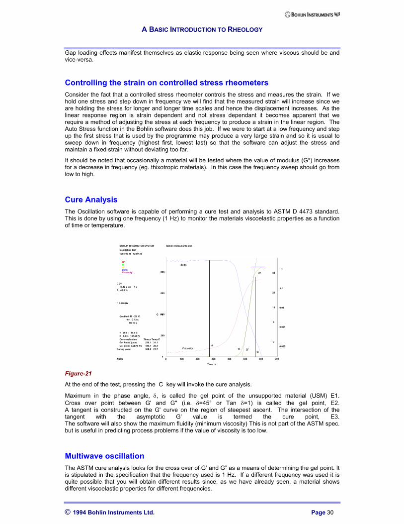
Cure AnalysisThe Oscillation software is capable of performing a cure test and analysis to ASTM D 4473 standard.This is done by using one frequency (1 Hz) to monitor the materials viscoelastic properties as a functionof time or temperature.

0

200

400

600

800

2

5

10

20

50

0.0001

0.001

0.01

0.1

1

0 100 200 300 400 500 600 700

Time s

G Pa

G*G'G"deltaViscosity*

t1t2

t3

BOHLIN RHEOMETER SYSTEMOscillation test1988-02-18 13:09:38

Bohlin Instruments Ltd.

C 2516.42 g cm 1 x

A 40.0 %

f 0.500 Hz

Gradient 40 - 20 C-0.1 C / 3 s

Mi 10 s

T 20.0 - 40.0 CR 0.03 - 121.99 %Cure evaluation Time,s Temp.CGel Point, (usm) 270.1 31.1Gel point 3.9E+0 Pa 440.1 25.4

Curing point 558.6 21.7

ASTM

delta

Viscosity G"

G'

Figure-21

At the end of the test, pressing the C key will invoke the cure analysis.

Maximum in the phase angle, δ, is called the gel point of the unsupported material (USM) E1.Cross over point between G' and G'' (i.e. δ=45° or Tan δ=1) is called the gel point, E2.A tangent is constructed on the G' curve on the region of steepest ascent. The intersection of thetangent with the asymptotic G' value is termed the cure point, E3.The software will also show the maximum fluidity (minimum viscosity) This is not part of the ASTM spec.but is useful in predicting process problems if the value of viscosity is too low.

Multiwave oscillationThe ASTM cure analysis looks for the cross over of G’ and G” as a means of determining the gel point. Itis stipulated in the specification that the frequency used is 1 Hz. If a different frequency was used it isquite possible that you will obtain different results since, as we have already seen, a material showsdifferent viscoelastic properties for different frequencies.



If we wish to study the viscoelastic properties as a function of frequency on a material that is changingwith time (or temperature) we must use some technique other than the discrete frequency methods wehave looked at so far. In a multiwave test, we generate a compound wave consisting of severalfrequencies summed together. This signal can then be used for discrete point measurements with thedata being displayed as frequency dependence as a function of time or temperature.

Rapid Frequency sweepsUsing multiwave, a frequency sweep only takes as long as the time to take a measurement at the lowestfrequency. Thus you can perform a 'frequency sweep' with many points at the low frequency end in afraction of the time it would take with a conventional frequency sweep.

The relative amplitude of each discrete frequency can be set, enabling you to ensure that the signalmeasured is within an acceptable range at each individual frequency. To assist in setting the relativeamplitudes, three functions are available which are used as follows:

Amplitude Use

Constant Solids1/f Viscoelastic materials1/SQRT(f) Liquids

The overall amplitude can either be set or the AutoStrain function used. Set this amplitude as you woulda normal single frequency ( i.e. to be in linear region ).



(C) RelaxationStress relaxation is a rather neglected technique that can give very useful information about viscoelasticmaterials. The test sample is subjected to a rapidly applied strain which is then held for the remainder ofthe test. The relaxation behaviour is then studied by monitoring the steadily decreasing value of shearstress. For a pure Newtonian material, the stress will decay instantaneously whereas for a pureHookean material there will be no decay. The simplest type of viscoelastic response is an exponentialdecay.

For long time scale tests the stress relaxation method is substantially faster than standard oscillationtesting to obtain the viscoelastic response as a function of time.

The stress relaxation test is also useful in quality control to obtain a ‘finger print’ which may indicateseveral rheological properties - viscosity, initial modulus and decay time.

(D) Stress GrowthThe stress growth test is the controlled shear rate rheometer’s counterpart to the creep test. Thesample is subjected to a linearly increasing strain normally over a long period of time. When the shearstress becomes constant as a function of time, the material is in steady state flow and the zero shearviscosity can be obtained. (Remember, in a creep test we have a fixed value of shear stress and wait forthe shear rate to become constant. The stress growth test applies a constant shear rate and waits forthe shear stress to become steady - thus the two tests are mathematically interchangeable)

The limitation of the stress growth test comes from the fact that the rheometer may not be able to applya sufficiently large enough strain to overcome the elastic component in the sample. Controlled stressrheometers can apply an infinite strain and so do not suffer from this problem.



APPENDIX-ASOME PRACTICAL APPLICATIONS OF RHEOLOGY

(A) Coatings

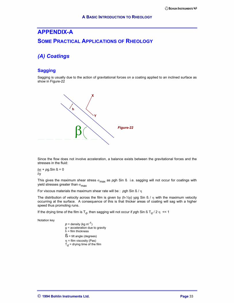
SaggingSagging is usually due to the action of gravitational forces on a coating applied to an inclined surface asshow in Figure-22

Figure-22

Since the flow does not involve acceleration, a balance exists between the gravitational forces and thestresses in the fluid:

δσ + pg.Sin ß = 0δy

This gives the maximum shear stress σmax as pgh Sin ß i.e. sagging will not occur for coatings withyield stresses greater than σmax

For viscous materials the maximum shear rate will be : pgh Sin ß / η

The distribution of velocity across the film is given by (h-½y) ypg Sin ß / η with the maximum velocityoccurring at the surface. A consequence of this is that thicker areas of coating will sag with a higherspeed thus promoting runs.

If the drying time of the film is Td, then sagging will not occur if pgh Sin ß Td / 2 η << 1

Notation keyp = density (kg m-1)g = acceleration due to gravityh = film thicknessß = tilt angle (degrees)η = film viscosity (Pas)Td = drying time of the film

β

X

Y

h



LevellingUnder certain conditions levelling depends upon the balance between the surface tension and viscousforces which oppose levelling. A sinusoidal film is produced as shown in figure-23

Figure-23

Analysing the equations of motion it can be shown that the film levelling occurs exponentially with timeaccording to :

h(t) = ho + a e-t/τ Sin (2π x / L)

The time constant τ is given by :

τ = 3 η L4 / ((2 π)4 σ ho3)

An approximate shear rate is :

Shear rateapprox. = 2a / Ln 2 τ L

This gives :

τmax = 8 π3 σ a h / L3

Notation keyh = ho + a Sin (2 π x / L)σ = surface tensionL = wave lengthτ = time constant

L

a

ho



SedimentationThe sedimentation velocity in a suspension is given by Stokes Law:

Vs = 2 r2 g (d-p) 9 η0

From this we find that the maximum shear rate obtained by the particles in the suspension is :

Shear ratemax = 3 Vs η0 2r

The limiting stress is thus given by :

σlimit = rg (d-p) 3

Thus, if the material has a yield stress greater than σlimit you will not have a problem with sedimentationotherwise the sedimentation rate can be determined from the maximum shear rate.

Notation keyr = particle radiusg = acceleration due to gravityp = density of suspending fluidd = particle densityη0 = Zero shear viscosity



Flow rates to shear rate conversionWhen pumping a material it is often useful to be able to predict the rate at which it will flow from anorifice. For a power law fluid (determine this by the Power law model in Data Processing) we can obtainvalues for the material constants k and n and use them as follows.

The shear rate will vary across the output nozzle and is zero at the centre of the jet. At the edge of thejet it is given by :

shear rateedge = 4Q

(πr3) (3/4 + 1/ 4n)

This equation can be used to check that k and n are being determined in the right range of shear rates.(As a first approximation you could set n=1 i.e. assume Newtonian behaviour, to get a rough idea ofshear rate range involved).

The flow rate from the tube orifice is determined by the pressure drop and the rheological properties kand n by means of the following equation :

Q = πr3 / (1/n + 3) x (Pr / 2k)1/n

Notation keyQ = flow rate (M3 S-1)r = radius of the tubeP = pressure gradient along nozzlek = from power law fitn = power law index (from power law fit)



(B) Polymers

Generation of heat in rapid oscillating deformation [5]

Materials undergoing rapid oscillating deformations will generate heat energy. An example of this is avehicle tyre travelling along an uneven surface. The following is an equation to predict the energydissipated per second from the material :

Σ° = w G" yo2 / 2 = wj"σo

2 / 2

Further information can be found in Ferry's book [5]

Notation keyyo = peak shear strainσo = peak shear stressw = angular velocity (2πf)

MWD and MW determinationFor many commercial polymer melts, it is generally accepted that the elasticity measured from a creeptest, Jo, is related to molecular weight distribution, independent of molecular weight. In contrast, it isalso generally accepted that the zero shear viscosity, ηo, is only a function of weight-average molecularweight (the higher the MW, the higher ηo)

It has been found that ηo is proportional to M3.4 over a considerable range of molecular weights formany polymers[6]

Consequently, creep (and creep recovery to give a more accurate Jo, see section 4) provide aconvenient way to separate the effects of molecular weight and distribution.

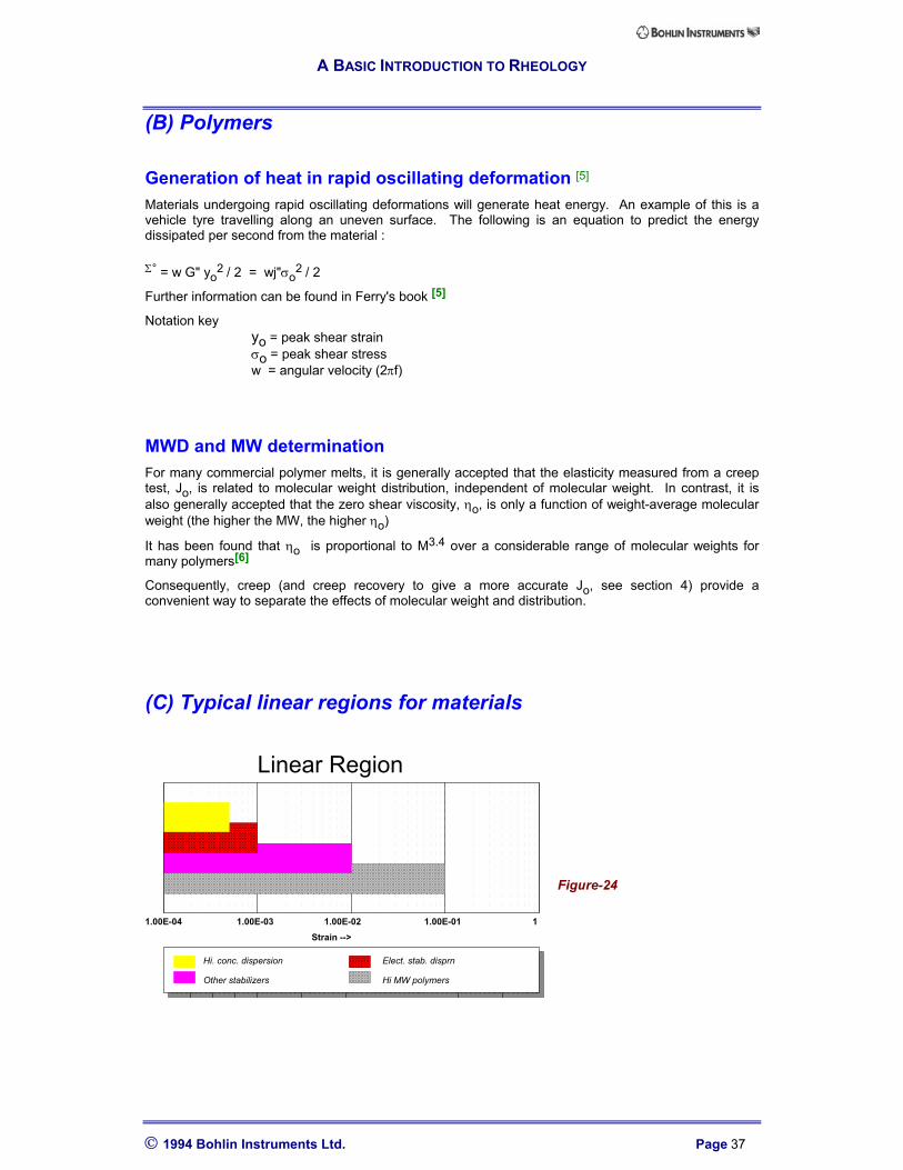
(C) Typical linear regions for materials

Figure-24

Linear Region

Strain -->1.00E-04 1.00E-03 1.00E-02 1.00E-01 1

Other stabilizers

Hi. conc. dispersion Elect. stab. disprn

Hi MW polymers



APPENDIX-BREFERENCES & BIBLIOGRAPHY

(A) References1 - Science Data Book, edited by R. M. Tennent, Oliver & Boyd ISBN 0 05 002487 6

2 - Adams, N and Lodge, A. S. (1964) Phil. Trans. Roy. Soc. Lond. A, 256, 149

3 - Taylor, G.I Proc. Roy. Soc. A157 546-578 [1936]

4 - Schrag J L Trans.Soc.Rheol. 21.3 (1977) 399-413

5 - Ferry, Viscoelastic properties of polymers (P.575)

6 - Ferry, Viscoelastic properties of polymers (P.379)

(B) BibliographyRheological Techniques - R. W. Whorlow (second edition, 1992)

Published by Ellis Horwood Limited, ISBN 0-13-775370-5

Viscoelastic Properties of Polymers - John D. Ferry

Published by John Wiley & Sons Inc. ISBN 0-471-04894-1

An Introduction to Rheology - H. A. Barnes, J. F. Hutton and K. Walters

Published by Elsevier Science Publishers B.V. ISBN 0-444-87469-0 (Paperback)



APPENDIX-CCALCULATION OF SHEAR RATE AND SHEAR STRESS FORMFACTORS.Rheometers and viscometers work with torque and angular velocity. Since we normally work with shearstress and shear rates a method is needed to convert from 'instrument numbers' to 'rheology numbers'.

Each measuring system used in an instrument will have its associated 'form factors' to convert torque toshear stress and to convert angular velocity to shear rate.

We will call the shear stress form factor C1 and the shear rate factor C2

Shear Stress = C1 x TorqueShear Rate = C2 x angular velocity *Viscosity = Shear Stress / Shear Rate

• For some measuring systems such as parallel plates, the gap between the measuring systems canbe set by the user. In this case the equation used is :

Shear Rate = C2 x angular velocity / gap.

The following section shows how the form factors are calculated for each measuring system.

(A) Cone and plateC1 = 3 C2 = 1 / θ

2 π r3

Where r = radius of cone θ = cone angle in radians

(B) Parallel platesC1 = 3 C2 = 3r / 4

2 π r3

Where r = radius of cone

NOTE: The shear stress varies across the radius for a parallel plate. The above formula refers to the 3/4radius position if the test sample is Newtonian.

(C) Coaxial cylindersC1 = 1 C2 = 2 ri2 ro2

2 π ra2 H ra2 (ro2 - ri2)Where ra = (ri + ro) / 2

ri = inner radiusro = outer radius H = height of cylinder

NOTE: C1 takes the shear stress as that occurring at an average radius position ra



APPENDIX-DPRINCIPLE OF OPERATION OF RHEOMETERS AND VISCOMETERS.The following information is based around the Bohlin range of rheometers and viscometers but shouldbe equally applicable to other instruments of similar types.

(A) Principle of operation of controlled stress (CS) rheometers

Figure-25

The principal components of a CS Rheometer are shown in figure-25. The rheometer is a constanttorque motor which works by a drag cup system. An angular position sensor detects the movement ofthe measuring system attached to the shaft.

The software automatically converts the applied value of torque to a shear stress when displaying data.The reading from the position sensor is converted to a strain, again by using the information about thecurrent measuring system. By monitoring the change of strain as a function of time we can obtain theshear rate.

Since the only data being produced by the rheometer is a deflection reading (from the angular positionsensor) it follows that the lowest shear rate you can achieve is determined only by how long you areprepared to wait, since the sensor must turn a measurable amount for the software to calculate a speedand hence a shear rate.

Position sensor

Measuring system chuck

Air bearing

Drag cup motor



(B) Principle of operation of controlled shear rate rheometers

Air bearing

Torsion bar

Position detector (LVDT)

Fluid jacket

Sample

Drive system

Figure-26

The principal components of a controlled rate rheometer are shown in figure-26. The rheometer is aconstant speed motor with a torque detection system.

The torsion bar is suspended on an air bearing to give a virtually friction less bearing. When the drivesystem turns, the sample resistance (viscosity) tries to twist the torsion bar. By measuring the resultanttwist and knowing the stiffness of the bar, the torque is measured.

The software automatically converts the measured torque to a shear stress when displaying data.



A

acetone............................................................ 5ageing ..................................................... 20, 22air.................................................................... 5ASTM D 4473.............................................. 30

B

Bingham ........................................... 13, 14, 15bitumen........................................................... 5brushing.......................................................... 5

C

Casson .......................................................... 14chewing .......................................................... 5coatings................................................... 12, 32coaxial cylinder .......................................... 8, 9compliance.................................. 18, 24, 25, 26computer....................................................... 21cone ................................... 6-10, 21, 23, 27, 38constant rate.................................................... 4creep ............................... 15, 24, 25, 26, 29, 36Cross....................................................... 14, 30cure ............................................................... 30curtain coating ................................................ 5

D

dashpot ..................................................... 4, 27Deborah number ............................... 24, 25, 29deformation ...... 3, 4, 15, 18, 24, 25, 27, 28, 36double gap ............................................ 8, 9, 10drag cup motor.............................................. 29drying ........................................... 8, 10, 26, 32

E

elasticity...................................... 18, 26, 27, 36Ellis......................................................... 14, 37equilibrium ................................. 18, 20, 24, 29extruding......................................................... 5

F

flow .............. 3-4, 11-16, 18- 22, 24-28, 32, 35fluid .......... 4, 11, 13, 21, 25, 28, 29, 32, 34, 35force.................................................. 3, 4, 5, 18

G

G' ............................................................ 28, 30gap Loading.................................................. 29glycerol........................................................... 5

H

Herschel Bulkley .......................................... 13Hookean ............................................. 3, 25, 27

I

inertia.............................................. 3, 9, 16, 29

K

Kelvin............................................................ 16

L

levelling ........................................ 5, 24, 25, 33linear region ............................................ 27, 30linear response .................................... 3, 27, 30loss modulus ................................................. 28

M

mixing ............................................................. 5models ............................................... 12, 13, 14Moore............................................................ 14

N

Newton.......................................................... 12Newtonian .............4, 11-16, 18, 25, 27, 35, 38

O

olive Oil .......................................................... 5oscillation.................................... 27, 28, 29, 30Ostwald model .............................................. 12

P

Pascal ................................................ 3, 4, 5, 28phase angle.................................. 27, 28, 29, 30plate............................. 6, 7, 8, 9, 10, 23, 27, 38polymers.......................................... 5, 7, 36, 37position sensor ........................................ 23, 39power Law .................................. 12, 13, 14, 35pumping .................................................... 5, 35

R

rheodestruction.............................................. 16rubbing............................................................ 5

S

sagging ................................................ 5, 24, 32sample Loading............................................... 8Schrag ..................................................... 29, 37sedimentation ...................................... 5, 24, 34shear rate ..... 2, 4-7, 9-16, 18-22, 25, 27, 29, 39shear strain .................................. 3, 4, 5, 27, 36shear stress ..... 2-5, 9, 11-15, 22, 24-27, 32, 36Sisko ............................................................. 14skinning................................................. 8, 9, 10spraying........................................................... 5spring ........................................................ 3, 27stirring............................................................. 5storage modulus ............................................ 28strain...... 3, 4, 15, 18, 22, 24, 25, 27, 28, 30, 39stress............. 3, 9, 13-15, 18, 19, 22, 24-30, 34

T

temperature ............................. 7, 10, 16, 20, 30thixotopy ....................................................... 16



torque.......................... 8, 18, 21, 29, 38, 39, 40

V

viscometry .................................. 11, 18, 21, 29viscosity.... 4, 5, 8-16, 18-23, 25, 27, 29-36, 38Vocadlo ........................................................ 13

W

water.......................................... 5, 6, 12, 16, 22

Y

yield .. 11, 13, 14, 15, 18, 19, 25, 26, 29, 32, 34



Date post:	24-Jun-2020
Category:	Documents
Upload:	others
View:	7 times
Download:	1 times

Manual: A Basic Introduction to Rheology Issue 2 › ... ›...

Documents