MARGINAL TAX RATES AND INCOME:NEW TIME SERIES EVIDENCE
Karel MertensJosé L. Montiel Olea
Working Paper 19171http://www.nber.org/papers/w19171
NATIONAL BUREAU OF ECONOMIC RESEARCH1050 Massachusetts Avenue
Cambridge, MA 02138June 2013, Revised September 2017
We thank the editor, Robert Barro, and the referees for their suggestions and comments, Daniel Feenberg for assistance with the US Individual Income Tax Public Use Sample, Glenn Follette for providing data, and Andrew Fieldhouse, Bryce Little, Qifan Han and Jianing Zhai for superb research assistance. We also thank Levon Barseghyan, Gregory Besharov, Lorenz Kueng, Kristoffer Nimark, Morten Ravn, Barbara Rossi and participants at various seminars and conferences for useful comments. Financial support from the Cornell Institute for the Social Sciences is acknowledged. The views in this paper are those of the authors and do not necessarily reflect the views of the Federal Reserve Bank of Dallas, the Federal Reserve System, or the National Bureau of Economic Research.
NBER working papers are circulated for discussion and comment purposes. They have not been peer-reviewed or been subject to the review by the NBER Board of Directors that accompanies official NBER publications.
Marginal Tax Rates and Income: New Time Series Evidence Karel Mertens and José L. Montiel OleaNBER Working Paper No. 19171June 2013, Revised September 2017JEL No. E6,E62,H2,H24
ABSTRACT
Using new narrative measures of exogenous variation in marginal tax rates associated with postwar tax reforms in the US, this study estimates short run tax elasticities of reported income of around 1.2 based on time series from 1946 to 2012. Elasticities are larger in the top 1% of the income distribution but are also positive and statistically significant for other income groups. Previous time series studies of tax returns data have found little evidence for income responses to taxes outside the top of the income distribution. The different results in this study arise because of additional efforts to account for dynamics, expectations and especially the endogeneity of tax policy decisions. Marginal rate cuts lead to increases in real GDP and declines in unemployment. This study also presents evidence that the responses are to marginal tax rates rather than average tax rates. Counterfactual tax cuts targeting the top 1% alone have short-run positive effects on economic activity and incomes outside of the top 1%, but increase inequality in pre-tax incomes. Cuts for taxpayers outside of the top 1% also lead to increases in incomes and economic activity, but with a longer delay.
Karel MertensDepartment of EconomicsCornell University404 Uris HallIthaca, NY 14853and [email protected]
José L. Montiel OleaColumbia UniversityDepartment of EconomicsOffice 10201022 International Affairs BuildingNew York, NY [email protected]
A data appendix is available at http://www.nber.org/data-appendix/w19171
1 Introduction
To what extent do marginal tax rates matter for individual decisions to work and invest? The answer is essential for
public policy and its role in shaping economic growth. The empirical literature studying US tax returns, surveyed in
Saez, Slemrod and Giertz (2012), concludes that reported pre-tax incomes react only modestly to marginal tax rates
and attributes evidence of larger responses for top incomes to tax avoidance rather than real economic effects. In
contrast, many macro studies find that indicators of real activity such as GDP, investment and employment respond
significantly to changes in taxes, e.g. Romer and Romer (2010), Barro and Redlick (2011) or Mertens and Ravn
(2013). This is puzzling, since the macro evidence for real economic effects of taxes should be apparent in market
incomes reported on tax returns.
This study reconciles the time series evidence on the aggregate responses to marginal tax rates by combining existing
macro methodologies with the reported income measures of Piketty and Saez (2003), as well as newly constructed
series on average marginal tax rates for the 1946-2012 period. Existing time series estimates of the elasticity of
reported income with respect to net-of-tax rates (one minus the marginal tax rate) are close to zero in the aggregate.
As a contribution to the public finance literature, we show that adopting specifications that address central concerns
related to timing, expectations, and in particular the endogeneity of tax policy, leads to statistically significant short
run elasticities centered around a value of 1.2 for all taxpayers.
At the core of the identification strategy are new measures of the impact of a number of federal tax reforms on
average marginal tax rates. The selection of tax reforms is based on the Romer and Romer (2009, 2010) narrative
account of postwar US tax policy, focusing on individual income and payroll tax changes implemented within a year
of their legislation to avoid anticipation effects. The tax elasticity estimates are obtained by using these measures
as ‘proxies’ for exogenous tax rate innovations in structural vector autoregressions as in Mertens and Ravn (2013),
or alternatively as instruments for tax rates in local projections similar to Barro and Redlick (2011). This paper
also contributes to the macro literature by developing the narrative identification approach for marginal rather than
average tax rate shocks, and by analyzing responses along the income distribution.
The regression results indicate that incomes in the top 1% of the income distribution display the strongest short
1
run response to tax rates, which is consistent with the notion that high income tax payers display more avoidance
behavior. However, contrary to prior time series studies of tax return data, we also find statistically significant elas-
ticities for lower income groups and narrower wage income measures. Moreover, marginal rate cuts lead to increases
in real GDP and declines in the unemployment rate that are broadly consistent with existing macro results. Simple
calculations suggest aggregate hours elasticities of 0.37 on the intensive margin and 0.41 on the extensive margin,
which is within the range of the quasi-experimental labor supply evidence surveyed in Chetty, Guren, Manoli and
Weber (2013).
In addition, we present new evidence to determine whether real economic activity responds primarily to marginal
tax rates, or to average tax rates. Combining measures of the impacts of the Romer and Romer (2009, 2010) reforms
on both, we estimate the consequences of counterfactual tax experiments that lead to an innovation in marginal tax
rates but not in average tax rates, and vice versa. We find that marginal rate changes lead to very similar income
responses regardless of the change in the average tax rate. There is, on the other hand, no evidence for any effect on
incomes when average tax rates decline but marginal rates do not. This implies that the reforms with a direct impact
on marginal tax rates are the key events generating the real economic effects estimated by the narrative macroe-
conometric studies. Our findings indicate that substitution effects, rather than income effects or aggregate demand
stimulus, are central to the transmission of federal tax policy changes observed in the postwar period.
Finally, we analyze the impact of counterfactual tax reforms cutting marginal tax rates only for the top 1% or the bot-
tom 99% in the income distribution. The associated short run reported income elasticity for the top 1% is estimated
to be around 1.5. In the short run, a top marginal rate cut in raises real GDP, lowers aggregate unemployment and
also has a measurable positive effect on incomes outside of the top 1%. Nevertheless, marginal rate cuts targeting
top incomes lead to greater income inequality. These results have implications for the interpretation of the observed
correlation between top marginal tax rates and top income shares, see Piketty, Saez and Stantcheva (2014). Causal
explanations based on avoidance or rent-seeking alone cannot explain the finding that top marginal rate cuts have
real economic effects and spill over to lower income groups. Targeted cuts for the bottom 99% also generate positive
effects on reported incomes and aggregate economic activity, but with a delay of several years. This delay may help
explain why broader responses to tax rates have been harder to detect empirically.
2
2 Income and Average Marginal Tax Rates
2.1 Existing Evidence on Income Responses to Taxes
The responsiveness of incomes reported to tax authorities, typically measured by the elasticity of taxable income, or
ETI for short, has received much attention as an indicator for the distortionary effects of taxes, see Saez, Slemrod
and Giertz (2012). The interpretation of an ETI measure depends on the definition of ‘taxable income’. As much of
the recent literature, we focus on broad measures of gross market income, i.e. before government transfer payments
and before the various adjustments and deductions allowed by the tax code. These broad ETI measures are generally
informative about the efficiency and revenue implications of tax policy changes, and can in some cases be used as a
sufficient statistic for optimal tax analyis.1
A large public finance literature has obtained quasi-experimental ETI estimates using US tax return data in a variety
of ways. The analysis of the 1981 reform by Lindsey (1987) used cross-sectional data and counterfactual income
simulations to document very large elasticities centered around 1.6. To better control for confounding factors, panel
data studies of the 1986 reform starting with Feldstein (1995) exploited heterogeneity in marginal tax rate changes to
establish treatment and control groups and make difference-in-difference comparisons. The combined evidence from
the 1980s reforms in Lindsey (1987), Feldstein (1995), Auten and Carroll (1995, 1999) and others pointed to large
short run ETIs in a range of 0.7 to over 3.0, although broadening the sample of taxpayers, the definition of income
or the set of controls yields estimates towards the lower end of that range. Subsequent event studies of reforms in
the 1990s, such as Sammartino and Weiner (1997), Carroll (1998) or Giertz (2010), instead obtained lower values
of close to 0 up to 0.5. This confirmed growing suspicions that the estimates for the 1980s were largely artifacts of
insufficient controlling and/or of certain attributes of these reforms leading to highly transitory effects, see Slemrod
(1995, 1996).
Diff-in-diff case studies, however, offer no definitive answer because there are many other determinants of rela-
tive income changes that are hard to control for and because it must be assumed either that there is no tax change for
the control group or otherwise that the ETIs are identical for both groups.2 To overcome some of these difficulties,
1See for instance Feldstein (1999), Saez (2001), Chetty (2009), Diamond and Saez (2011) or Badel and Huggett (2015).2Blundell et al. (1998), Slemrod (1998), Triest (1998), Goolsbee (1999) and Saez et al. (2012) discuss the empirical issues.
3
one strategy is to assume ETIs are roughly time-invariant and cumulate evidence from a number of tax reforms.3 Em-
pirical models that under reasonable assumptions restrict unobservable confounding influences on income growth to
have zero mean allow for averaging out those influences over time. For instance, Gruber and Saez (2002) use a long
panel dataset from 1979 to 1990 to exploit richer variation in tax rates during that period and find an elasticity of in-
come (before deductions and exemptions) of close to zero in the sample of all tax returns. Starting with Feenberg and
Poterba (1993), most studies adopting a broader time perspective, however, use more aggregated data that is available
for different and/or longer sample periods. By gathering evidence from multiple reforms, such studies have further
confirmed the view that the reported income responses observed for the 1980s reforms were anomalies. In time series
regressions of top income shares on net-of-tax rates over the 1950-1990 period, Slemrod (1996) for instance finds
that the elasticity drops considerably when the last five years containing the 1986 reform are excluded. Goolsbee
(1999) uses aggregate data to obtain separate short run diff-in-diff elasticities for seven reforms between 1920 and
1975 and finds that the largest estimate is far below those for the 1980s reforms. In aggregate time series regressions,
Saez (2004) and Piketty, Saez and Stantcheva (2014) find small and statistically insignificant elasticities for all tax
units and moderate but significant elasticities for top incomes. Collecting diff-in-diff evidence from reforms during
the interwar period, Romer and Romer (2014) find elasticities for top incomes around 0.20. In their survey of the
available evidence, Saez, Slemrod and Giertz (2012) acknowledge there are no truly convincing estimates of long run
ETIs but conclude that the best available estimates are in a range of 0.12 to 0.40. There is much evidence for larger
short run ETIs for high income tax payers which they attribute mostly to better access to avoidance opportunities.
Beyond that, Saez et al. (2012) argue, there is no compelling evidence for any real economic responses to marginal
tax rates.
The conclusions from the ETI literature are at odds with the recent macro empirical literature that exploits pol-
icy reforms as quasi-experiments to identify the effects of taxes on aggregate real economic variables such as GDP,
unemployment or investment. Starting with Romer and Romer (2010), ‘narrative approach’ studies have consistently
estimated substantial short and medium run effects of taxes on economic activity. For instance, Romer and Romer
(2010) find that a policy-induced increase in federal tax liabilities of 1% of GDP lowers GDP by 3% and investment
3Another strategy is to look for features in the tax code that generate differential tax rates for narrower but more similar groups oftaxpayers. Unfortunately the results may not be more broadly representative and, while the case for identification may become moreconvincing, the identifying variation in tax rates is typically smaller. Taxpayers may not be aware of the minute details of the tax codeand/or have insufficient incentive to respond to small changes, see Chetty (2012). The findings may therefore be less relevant for largerchanges in marginal tax rates.
4
by 9% after two years. Mertens and Ravn (2013) find that a one percentage point decrease in the personal average
tax rate raises GDP by 1.5% and lowers the unemployment rate by 0.5 percentage points within a year. Also using
tax reforms for identification, Cloyne (2013) and Hayo and Uhl (2014) find remarkably similar results for the UK
and Germany, while Leigh, Pescatori and Guajardo (2014) find large contractionary effects of tax based fiscal con-
solidations in OECD countries. The lack of evidence for real substitution effects in the ETI literature is also puzzling
in light of a closely related labor supply literature that uses tax experiments and hours or employment as outcome
variables. Based on their reading of the recent evidence, Chetty, Guren, Manoli and Weber (2013) view elasticities
of aggregate hours of 0.5 for a permanent tax change and 0.75 for a transitory tax change as realistic. As broader
measures of the behavioral response, ETIs should be at least as large as these labor supply elasticities.
The conflicting evidence on the real effects of taxes between the ETI and macro literatures cannot be easily re-
solved by any of the explanations for the gap between micro and macro labor supply elasticities, since the public
finance evidence includes analyses of aggregate time series.4 One potential explanation is that most of the macro
studies focus on average rather than marginal tax rates. Many reforms impact differently on both and any aggregate
demand effects due to changes in disposable income may feature more prominently in the macro estimates. Using
the Romer and Romer (2009, 2010) tax policy measure as an instrument, Barro and Redlick (2011) however find that
a one percentage point cut in the AMTR raises per capita GDP by around 0.5% in the following year. This estimate
is statistically significant and amounts to a short run GDP elasticity to the net-of-tax rate of 0.36, which should be a
lower bound for the elasticity of personal income. By comparing results from specifications with average tax rates,
Barro and Redlick (2011) also tentatively conclude that the response is mainly to marginal rather than average tax
rates.
The main objective of this paper is to investigate the main claims of both the ETI and macro literatures on the
real effects of tax changes and expose the sources of the disagreement. To include more historical variation in tax
rates, we employ newly extended time series on postwar AMTRs that are discussed next.
4See Keane and Rogerson (2012) and Chetty et al. (2013) for the debate on micro and macro labor supply elasticities.
5
2.2 Average Marginal Tax Rates 1946-2012: Description and Stylized Facts
Figure 1 depicts estimates of annual US average marginal tax rates from 1946 to 2012 for the aggregate economy
and within different income brackets. The series combine federal individual income tax rates and contribution rates
under the Old-Age, Survivors and Disability Insurance and Medicare Hospital Insurance programs. The tax rates and
income rankings reflect the population of potential tax units, defined as all married men and singles aged 20 or more.
The upper panel of Figure 1 shows two AMTR measures for all tax units that differ primarily in the income concept
used for weighting. The first measure is based on a broad concept of labor income used by Barro and Redlick (2011)
that includes wages, self-employment, partnership, and S-corporation income. The other aggregate series, as well as
the series for top and bottom tax units in the lower panel of Figure 1, use an income concept from Piketty and Saez
(2003) that includes non-labor income but excludes capital gains and government transfers. The percentiles are for
the distribution of the Piketty and Saez (2003) definition of income across potential tax units.5
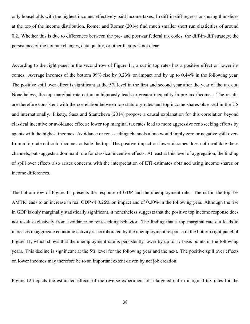
Figure 2 shows the income tax component. The first series for all tax units updates the measure of Barro and
Redlick (2011) to include observations post 2006. The series based on the Piketty and Saez (2003) income concept
extend those of Saez (2004) by almost 30 years using data from the IRS Statistics of Income. The social security tax
rates in Figure 3 are constructed from data published by the SSA, as well as individual IRS tax returns. The series
for all tax units are updates of Barro and Sahasakul (1986). The series for top and bottom tax units are entirely new.
Appendix A provides full details on the construction of the tax rates. One limitation of the series is that social secu-
rity benefits depend partially on earnings. In principle, marginal changes in benefits should be netted out to obtain
the tax component. In practice the inclusion of social security has no major implications for the results in this paper.
Another limitation is that the series do not include state-level taxes. The amount of short run variation in aggregated
state-level marginal tax rates is very small, see Barro and Redlick (2011), such that this omission is unlikely to be
important.
The tax rates for all tax units in Figure 1 display an upward trend starting at around 20% right after WWII and
rising to over 35% at the beginning of the 1980s. The main source of this trend is the gradual expansion of social
5Piketty and Saez (2003, 2007) provide a detailed description of the income data, which for most years is based on public use filescontaining around 100,000 returns. In the postwar period, the top 1% income share was about 11% after the war, declined to 8% in the1960s and 1970s and has gradually risen since to about 19% in 2012. The top 10% share was about 1/3 after the war and has risen since thelate 1970s to about 48% in 2012.
6
security contributions from less than 1% in 1946 to around 9% since the early 1990s, see Figure 3. The upward
trajectory accelerates in the 1970s because of rapid increases in income tax rates primarily due to high inflation and
bracket creep. In the 1980s, the continuing rise in social security rates is largely offset by decreases in income tax
rates. The income tax component appears stationary over the postwar period and is typically in the 20%-25% range.
The tax rates by income in the lower panel of Figure 1 show a substantial decline in progressivity after 1980. This
decline is mostly the result of reforms in the 1980s but also partly due to the growing importance of the regressive
social security tax, which taxes individual earnings above a statutory ceiling at a zero marginal rate before 1994 and
only at the lower hospital insurance rate afterwards.
In the short run, the tax rate series in Figure 1 display substantial variation that is predominantly driven by in-
come taxes. The larger annual fluctuations in income tax rates reflect well known legislative changes.6 Because
brackets and ceilings are imperfectly indexed, AMTRs also vary automatically with nominal income levels even in
the absence of legislative changes.7 Changes in the social security rates are less important for the year-to-year vari-
ability in overall rates.8 To provide more insight into the sources of annual variation in tax rates, Figure 4 depicts
estimates of the impact of policy driven statutory changes in overall tax rates (upper panel), as well as in the income
tax and social security rates individually (lower left and right panels). The estimated statutory component in year
t is calculated as the difference between a counterfactual average marginal tax rate, calculated using the year t− 1
income distribution and year t rates and brackets deflated by any automatic adjustments between t−1 and t, and the
actual year t−1 average marginal tax rate. The difference between actual and policy induced annual changes in tax
rates thus captures the effect on AMTRs of the change in the income distribution relative to the previous year. This
is of course only an ‘effect’ in a purely accounting sense and should not be given a causal interpretation.
6The most significant adjustments include the rate reductions in 1948 following the end of WWII, the tax increases in the 1950s duringthe Korean War; the 1964 Kennedy tax cuts; the 1968-1970 surcharge during the Vietnam War; the 1980s Reagan tax cuts and in particularthe 1986 Tax Reform Act; the early 1990s Bush and Clinton tax increases; and the W. Bush tax cuts in the early 2000s.
7Annual inflation adjustments to income tax brackets began only in 1985 and to date there is no real income indexation. De facto inflationadjustments started in 1985 although automatic indexing to the CPI did not begin until 1987. Some components of the tax code, such as thealternative minimum tax, have not been automatically indexed to inflation even after 1987. The American Taxpayer Relief Act of 2012 startsautomatic indexation of the alternative minimum tax in 2013. All indexation occurs with significant delay and is applied roughly uniformlyacross the income distribution.
8Social security contributions depend on taxable maxima that have been automatically indexed to national average wage growth startingin 1975. The many statutory changes to social security contribution rates and/or taxable earnings prior to the early 1990s are all permanentand gradual increases that are comparatively smaller in size. The most noticeable changes result from the Great Society initiatives underJohnson including the introduction of Medicare in 1966, the 1972, 1977 and 1983 amendments of Social Security and the expansion of theMedicare tax in the early 1990s. The only reduction is the temporary cut in contribution rates under Obama in 2011 and 2012.
7
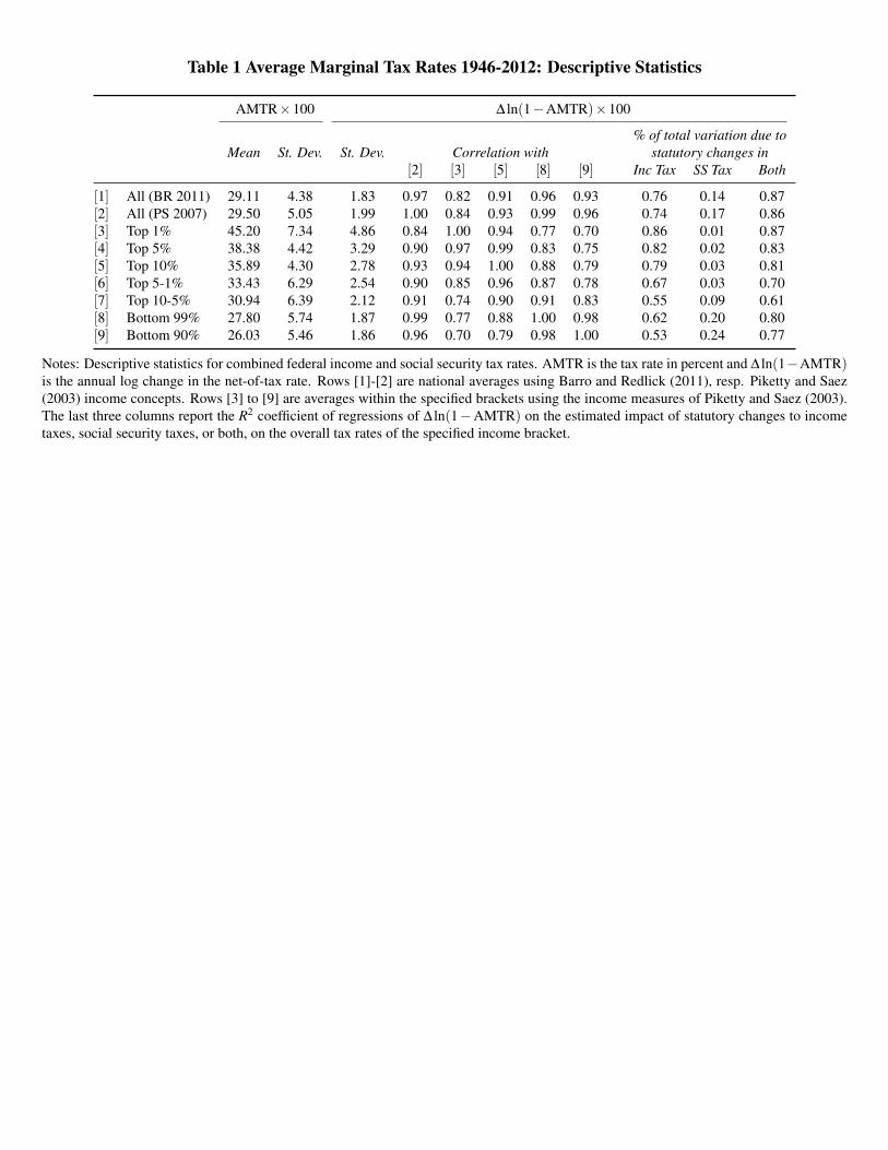
Table 1 quantifies some key characteristics of the combined AMTR series in Figure 1 and the sources of varia-
tion. The first eight columns provide first and second order properties of the tax rate levels and of changes in the
net-of-tax rates by income group. The last three columns in Table 1 contain the contribution of statutory changes to
the overall variation in annual net-of-tax rate changes. These are measured by the R2 coefficient of regressions of
net-of-tax rate changes on the statutory changes estimated for each income group separately as described above, i.e.
by constructing a counterfactual tax rate that keeps the income distribution fixed and adjusts for automatic indexation.
Table 1 reveals a number of important features of the tax rate series. First, there is substantial variation in post-
war AMTRs, most of which is driven by policy changes. The raw standard deviation of annual changes in net-of-tax
rates for all tax units is 1.8% to 2.0% . More than 85% of the variation is explained by statutory changes. Second, the
federal income tax is the dominant source of fluctuations in income-weighted tax rates. Three quarters of the varia-
tion in net-of-tax rates for all tax units is explained by legislative changes to income taxes, whereas statutory changes
in social security taxes account for 14% to 17%. Third, there is considerable heterogeneity in tax rate variability
across income groups. Annual percentage changes in net-of-tax rates are considerably more volatile for top incomes
than for lower incomes, explaining 80% or more of the total variation. Not surprisingly, statutory changes in social
security taxes contribute very little to the variation in top tax rates. For the bottom 90% and 99% groups, statutory
social security changes on the other hand explain up to one fifth, respectively a quarter of the variation whereas
statutory income tax changes account for up to 62%, respectively 53%. Fourth, the AMTRs remain very highly
correlated across large sections of the income distribution. The lowest correlation, between the top 1% and bottom
90%, is 0.70. The income specific AMTRs are all highly correlated with either of the series for all tax units: even the
top 1% AMTR has a correlation of over 0.80 with the aggregate for all tax units. Finally, the two AMTR measures
for all tax units are very highly correlated and none of the results below are very sensitive to which measure is chosen.
The initial analysis of the tax rates highlights some of the advantages and challenges of using aggregate time series
to identify tax elasticities. The full postwar history of federal tax legislation clearly offers a rich amount of potential
identifying variation and includes many large increases and decreases in tax rates. Policy-induced fluctuations in
tax rates are especially large at the top of the income distribution. A longer time series perspective can therefore be
particulary revealing about the behavioral responses of high income taxpayers in a way that is not too dependent on
8
any particular reform. At the same time, the dominant role of the income tax in the variability of income-weighted
tax rates means that any results are likely to be representative only for the middle and higher income classes. Many
low income households have no federal income tax liabilities and variation in social security contributions is more
limited. The large cross-correlations of tax rates among income groups also point to a potentially important role for
general equilibrium effects in shaping the income response to tax rates. The vast majority of federal tax reforms are
aggregate events that may influence the wage distribution, monetary policy and interest rates, or other fiscal policy
instruments such as government spending and corporate and other taxes. In reality, the tax transmission mechanism
is complex and ETI estimates based on aggregate series do not lead directly to any strong conclusions about micro-
level elasticities. On the other hand, macro elasticities that incorporate all these effects provide a more complete
measure of the ultimate distortionary effects of marginal tax rates that is useful for evaluating tax policies in practice.
3 Preliminary Elasticity Estimates from Basic Time Series Regressions
Before proceeding to the main analysis, it is useful to first consider some preliminary regressions that establish that
the broader coverage of the income weighted tax rate series alone does not change the key conclusions of existing
studies that use similar aggregate data. Saez (2004), Saez et al. (2012) and Piketty et al. (2014) estimate aggregate
elasticities in time series regressions of income (before deductions and exemptions) in levels or top income shares on
net-of-tax rates and polynomials of time. Using AMTR series covering 1960-2000 and including linear and quadratic
trends, Saez (2004) finds an elasticity for all tax units of 0.20 that is not statistically significant. Separate regressions
by income group result in a highly significant value of 0.50 for the top 1% and zero for the bottom 99%. Using the
top 1% income share instead of the level and adding a cubic time trend, Saez et al. (2012) obtain a highly significant
top 1% elasticity of 0.58 in the 1960-2006 sample. Piketty et al. (2014) use series for top statutory rates from 1913 to
2008 and obtain highly significant top 1% ETIs of 0.27 and 0.30 in the level and share regressions with a linear trend.
Using our extended 1946-2012 AMTR series and the same regression specifications, we obtain a tightly estimated
top 1% elasticity close to 0.60 in the level and share regressions and lower insignificant values in the others.9 As in
Saez (2004), we also find that instrumenting with statutory changes to avoid endogeneity related to tax progressivity
has little effect on these results. Static regressions with basic time controls therefore continue to produce results in
9In the 1946-2012 sample, the Saez (2004) level regressions yield values of 0.30 for all tax units, 0.61 for the top 1% and 0.37 forthe bottom 99%. Only the top 1% estimate is statistically significant. The top 1% share regression of Saez et al. (2012) yields a highlysignificant value of 0.59 in the full sample. As in the original papers, we used AMTRs for the federal income tax only.
9
line with a zero or small overall response and a moderately large response at the top. The latter, remains outside of
the range obtained in the short run for the 1980s reforms.
Unfortunately, there are two broad reasons why these regressions do not yield reliable estimates of the aggregate
causal effect of tax rates on reported income. The first reason is the failure to account for the dynamics of tax rates
and the timing of the behavioral response. The second reason is the endogeneity of tax policy decisions.
If tax rate changes are permanent, the elasticity in level regressions measures the eventual long run response and
should be insensitive to timing. If tax rates changes are instead transitory, than the timing of the income response
becomes very important. In reality, many tax reforms affect tax rates only temporarily by including sunset provisions
or because of subsequent reforms in the opposite direction. In the extreme case where tax rates are uncorrelated over
time, the regressions will detect no effects if, for instance, the income response occurs entirely in years before or after
the tax change. Any measurable response is likely to be partially delayed in practice, which can lead to a downward
bias in the elasticity estimate. One reason is that statutory tax changes occur throughout the year before filing, such
that the full income response may not be observed until the first year following the change. In addition, tax rates
may also impact on investment and other dynamic decisions with lagged effects on reported incomes. There are also
good reasons to believe that income responses partially lead tax rate changes. Many statutory tax rate changes are
phased in gradually over multiple years or are implemented with long delays.10 In response to future changes in
marginal tax rates, forward looking agents have incentives to allocate income generating activities optimally across
time. There is indeed substantial empirical evidence for such anticipatory effects to taxes.11 The sign of the bias due
to tax foresight is ex ante ambiguous and depends on the relative strength of intertemporal substitution versus income
effects, among other things. Regardless, the complicated intertemporal linkages between tax rates and incomes cast
doubts on the results from the static regressions.
The other major concern is that OLS or IV regressions with statutory tax rate changes as instrumental variables
10This is the case for instance for the marginal rate changes under the Revenue Act of 1964, the Economic Recovery Tax Act of 1981, the1986 Tax Reform Act or the Economic Growth and Tax Relief Reconciliation Act of 2001. Most adjustments to social security contributionrates have been implemented with multi-year lags.
11Kueng (2014) finds evidence in municipal bond yields that financial markets forecast federal tax rates remarkably well. The publicfinance literature documents anticipatory effects for a number of reforms, see Saez, Slemrod and Giertz (2012). For theory and evidence ofreal anticipatory effects, see Yang (2005), House and Shapiro (2006), McGrattan (2012), Mertens and Ravn (2012) and Leeper, Walker andYang (2013).
10
do not address the endogeneity of tax policy itself. Legislative reforms have a variety of motivations that are hardly
independent of other influences on incomes or income shares. Tax policy has been actively used for macroeconomic
stabilization and has systematically responded to temporary changes in military spending or other budgetary needs.12
Given a relatively broad consensus for expansionary effects of government spending, see Ramey (2011b), both chan-
nels make tax rates procyclical and induce a downward bias in the elasticity estimates.13 Bracket creep also remains
an important source of reverse causality. Three of the largest rounds of statutory income tax rate cuts (part of reforms
in 1964, 1981 and 2001) each followed periods of substantial bracket creep and effectively restored tax rates to his-
torical averages.14 Sectoral shifts, demographic trends, trade policies or changing political preferences are among
the many other possible factors that simultaneously shape the income distribution and tax policy decisions. Static
regressions with time polynomials are unlikely to control for even the most important of all of these confounding
factors.
To address some of these issues, we follow Slemrod (1996) and adopt specifications that include dynamic terms,
as well as a number of control variables. The reported income measures are in constant 2010 dollars per tax unit
and are the same as in Piketty and Saez (2003, 2007). These measures include all sources of market income before
deductions and exemptions but exclude realized capital gains and government transfers. The tax rates are those in
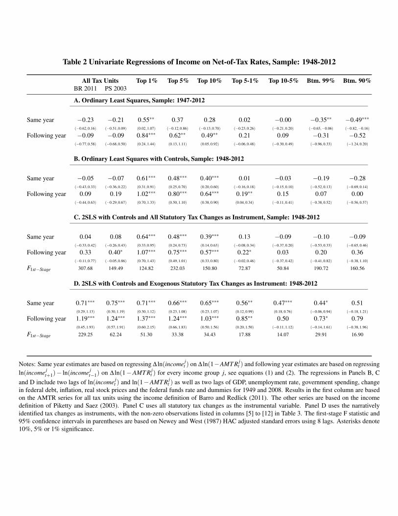
Figure 1 and include federal payroll taxes. Table 2 shows results for regressions of changes in log income on changes
in the log net-of-tax rate of income group j:
∆ ln(income jt ) = β∆ ln(1−AMT R j
t )+ [controls]+ut , and (1)
ln(income jt+1)− ln(income j
t−1) = γ∆ ln(1−AMT R jt )+ [controls]+ vt . (2)
12The Revenue Acts of 1950 and 1951 increased taxes to finance the war efforts in Korea. The Revenue and Expenditure Control Act of1968 imposed a temporary 10 percent surcharge to prevent the economy from overheating and finance the escalation of the Vietnam war.The Tax Relief Reconciliation Act of 2001 introduced a new 10% low income tax bracket to cushion the economic slowdown. The vastmajority of increases in social security rates fund benefit expansions. The temporary cut in contribution rates under Obama in 2011 and 2012was motivated by the continued weakness in the US economy. See Pechman (1987) or Romer and Romer (2009) for historical backgroundand more examples.
13Parker and Vissing-Jørgensen (2010) document the procyclicality of top income shares. Ceteris paribus, procyclical tax rates then leadto downward bias for higher incomes also in income share regressions.
14Figures 2 and 4 (lower left panels) show that, while there were no major statutory income tax increases in the 1970s, high inflation andbracket creep caused AMTRs to rise by 6 to 8 percentage points. The 1955-1963 period and the mid to late 1990s also saw no significantlegislative changes but rising tax rates due to (mostly real) increases in incomes.
11
where ∆ denotes the annual difference. By using differences instead of levels, these regressions now explicitly aim
for short rather than longer run elasticities. The first equation includes annual reported income and tax rate changes,
whereas the second equation uses two year income growth as the regressand. To the extent a tax change persists into
the subsequent year, the second regression potentially produces a more meaningful short run estimate by measuring
the income response after the first full year following a tax change, see also Barro and Redlick (2011). We focus on
income levels rather than income shares primarily because of the high correlations of tax rates among the income
groups and all of the prior evidence that elasticities vary with income. Another reason not to use income share re-
gressions is the potential for spill-over effects of tax rate changes for one group on incomes in others.
Panel A first presents results for the regressions in (1) and (2) without including any additional controls. This
yields short run elasticities that range from 0.55 for the top 1% to −0.49 for the bottom 90% in the same year of the
tax change, and elasticities of 0.84 for the top 1% to−0.52 for the bottom 90% in the following year. As before, only
for top incomes is there evidence for positive elasticities that are statistically significant at conventional confidence
levels. The ETIs outside the top 1% and for all tax units are generally not significantly different from zero at either
horizon. For the bottom 90% and 99% the same year estimates are significantly negative, suggesting that tax rate
increases lead to higher income growth in those groups. To mitigate concerns about timing and endogeneity, Panel B
includes two lags of income and net-of-tax rates of group j, as well as a large number of other lagged macroeconomic
variables as controls.15 The predetermined variables are assumed to jointly contain information about the relevant
history of events before time t that determine income and tax rates from time t onwards. These past events include
tax rate changes, announcements of future tax rate changes, cyclical and other fiscal shocks or any other relevant
causal factors that continue to influence current and future income and tax rates. Panel C instruments with the statu-
tory changes in Figure 4 to further correct for any contemporaneous influence on income that also has an effect on
tax rates because of progressivity. The results in Table 2 show that adding controls and instrumenting with statutory
changes each raises the point estimates relative to the simple OLS estimates. The subsequent year top 1% elasticity
increases to just above one in both panels B and C and instrumentation results in some evidence for a significant
effect also in the top 5 to 1%. The point estimates for the bottom 99% and 90% become positive or only mildly
negative but remain insignificant. The first stage F-statistics are large in all cases, which is not surprising given that
15To make a clear comparison, the control set is identical as in the vector autoregressions and local projections of Section 4 and includestwo annual lags of real GDP, the unemployment rate, inflation, the federal funds rate, government spending, the change in government debtheld by the public and the real stock market price, as well as dummies for 1949 and 2008.
12
changes in AMTRs are predominantly due to statutory changes.
One conclusion from panels A, B and C in Table 2 is that switching to a short run specification and including
richer controls raises the top 1% ETI from 0.6 to around 1. Despite being based on the entire postwar sample, this
value is now more firmly in the range of short run responses associated with the 1980s reforms, which contradicts
the view that these reforms were large anomalies. At the same time, the main conclusions of Saez (2004), Saez et al.
(2012) and Piketty et al. (2014) remain intact. Moving outside of the top 1% or 5%, the elasticities drop off sharply
and are generally insignificant. Based on the results in Table 2, the evidence for a sizeable response outside the top
1% or in the aggregate appears weak or nonexistent. The relatively large short run elasticities for the top 1% also
do not contradict more modest long run responses. As Slemrod (1995, 1996) has documented for the 1986 reform,
much of the short run response at the top may be due to transitory timing and avoidance effects rather than changes
in real economic activity.
The main problem is that none of the reported income regressions discussed above resolves the endogeneity of
tax policy. If any of the contemporaneous influences on income, such as cyclical or budgetary shocks, also system-
atically influences tax policy, then reverse causality remains a concern. The next section shows how the narrative
approach of Romer and Romer (2010) can be used to address the endogeneity of tax policy, and that reverse causality
concerns have important implications for ETI estimates based on aggregate time series.
4 Dynamic Estimates of the Income Response to Marginal Tax Rates
This section presents ETI dynamic estimates from structural vector autoregressive models (SVARs) and local pro-
jections (LP). In both cases, we identify the dynamic causal effects of exogenous tax policy interventions using
narrative measures of exogenous variation in MTRs as a proxy variable/external instrument for policy shocks. Fol-
lowing Stock and Watson (2017), we refer to the joint use of SVAR or LP estimators and instrumental variables
techniques as SVAR-IV and LP-IV, respectively.
The SVAR-IV/LP-IV analyses differ from univariate regressions in several ways. First, both approaches empha-
size the need for including a sufficiently rich set of lagged macroeconomic controls to isolate unanticipated variation
13
in both tax rates and reported income. Second, neither of the two methodologies assumes that all statutory changes
in tax rates are exogenous; instead, they rely on a selection of policy reforms that are not driven by other contem-
poraneous events, such as recessions or wars, and that are not fully anticipated. Third, both approaches include a
variety of other variables in a dynamic system, which enables the estimation of the full dynamic income effects and
allows for general feedback mechanisms. In fact, both models allow us to identify the expected future trajectory of
tax rates, which is important for interpreting ETI estimates. Finally, by including GDP and the unemployment rate
as endogenous variables, SVAR-IV and LP-IV estimates reveal whether reported income effects are also associated
with important changes in real economic activity.
4.1 SVAR-IV Methodology
Introduced by Sims (1980), SVARs are flexible time-series models that have been influential for evaluating the effects
of monetary and fiscal policy interventions.16 Consider the following VAR representation for aggregate income and
the marginal tax rate:
− ln(1−AMT Rt)
ln(incomet)
Xt
= d +A(L)
− ln(1−AMT Rt−1)
ln(incomet−1)
Xt−1
+
uAMT Rt
uincomet
uxt
, (3)
where Xt is a vector of control variables of dimension dx, A(L) is a p−1 lag polynomial and p is the lag length.
The key assumption of an SVAR model is that the forecast-errors of (3) are a linear combination of a vector of
structural exogenous shocks vt ; that is: uAMT R
t
uincomet
uxt
= Bvt , (4)
with E[vt ] = 0 and E[vtv′t ] a diagonal matrix. We partition the vector of structural shocks as:
vt ≡ [vτt , (v
ot )′ ]′, (5)
16See Ramey (2016) for a recent survey.
14
where vτt is a scalar shock that represents exogenous innovations in tax rates and vo
t is a vector containing all other
structural shocks that affect the economy. A standard assumption is that there are (at least) as many shocks as en-
dogenous variables: dim(vot )≥ dim(Xt)+1. The validity of (4) is in practice determined by the selection of variables
included in Xt and the lag length p. An appropriate choice of Xt and p ensures that the VAR residuals correspond to
unpredictable variation in the variables and therefore that all anticipated changes in marginal tax rates are controlled
for.
In the SVAR model, the contemporaneous responses of average marginal tax rates, aggregate income, and con-
trol variables to exogenous changes in vτt are captured by the first column of the matrix B, denoted B1. We normalize
B1,1 = −1, so that the baseline shock of interest is one that decreases − ln(1−AMTRt) in one unit upon impact,
corresponding to a cut in tax rates. The k-th period ahead dynamic response of variable i can be traced out using (3),
following the formulae in Lutkepohl (1990), p. 116, equation (3).
The VAR residuals uAMT Rt , uincome
t and uxt can be estimated by least-squares, but more assumptions are needed to
identify the responses to exogenous innovations to tax rates vτt . The identification strategy follows exactly Mertens
and Ravn (2013, 2014) and Stock and Watson (2008, 2012) and relies on the availability of an proxy variable/external
instrument zt for the latent structural tax shock vτt that satisfies the identifying assumptions:
E[ztvot ] = 0 (SVAR-IV exogeneity), (6)
E[ztvτt ] = α 6= 0 (SVAR-IV relevance). (7)
The first condition states that zt is contemporaneously correlated with the shock to marginal tax rates vτt . The second
condition requires zt to be contemporaneously uncorrelated with all other structural shocks contained in vot . When
these conditions hold, the dynamic responses to exogenous tax rates innovations are identified up to scale by the
covariance between zt and the VAR residuals:
E[ztut ] = αB1, (8)
15
with ut = [uAMT Rt
′,uincome
t′,ux
t′]′. Thus, the variable zt can be used to obtain a consistent estimator of B1 by regressing
each of the entries of ut on −uAMT Rt using zt as an instrument.17 Section 4.3 describes the variable zt used to identify
the dynamic responses of income and other macroeconomic variables to changes in marginal tax rates.
4.2 LP-IV Methodology
The LP-IV approach combines the method of local projections to estimate impulse response functions, as proposed
by Jorda (2005), with the use of instrumental variables for identification.18 In contrast to the SVAR model, the local
projections do not impose vector autoregressive dynamics for marginal tax rates or income.
Let Yt+k denote the (t + k)-th value of some macroeconomic variable of interest and let Wt be a vector of control
variables available at time t. The baseline LP-IV specification estimates the dynamic response of Yt+k to changes in
the marginal tax rates at time t is based on the model:
Yt+k = a+b′Wt + IRFk log(1−AMT Rt)+ et . (9)
By construction, the error term in (9) contains all contemporaneous, past, and future shocks that affect the best linear
prediction of Yt+k beyond the marginal tax rate and the vector of control variables (both at time t). This interpreta-
tion compromises the typical exogeneity assumption made in linear regression models: since the AMTR is a policy
variable it can respond to the present, past, and future state of the economy. Thus, the log net-of-tax rate can be
correlated with the error term.
To estimate the parameter IRFk in (9), the key assumption made in the LP-IV framework is that the random variable
zt is an exogenous and relevant instrument for the average marginal tax rate in the conventional sense; that is:
t .18See Ramey (2016), Ramey and Zubairy (2017), or Stock and Watson (2017) for discussions and recent applications of this approach.
16
where a⊥t denotes the residual of the population’s best linear prediction of at on a constant and the controls Wt .
Conceptually, it is possible to think of the exogeneity assumption for zt as imposing three different conditions. First,
zt has to be contemporaneously exogenous. This condition requires us to focus on a subset of tax reforms that are not
systematically related to other concurrent macroeconomic events. Second, zt has to be lag exogenous. This condition
requires zt to be uncorrelated with all past information contained in et . For this condition to hold, the selection of
control variables is crucial. For example, if zt includes tax reforms that respond to inherited deficit concerns (as it is
in our case), Wt has to be such that the past shocks that remain in et are uncorrelated with zt . Finally, zt has to be lead
exogenous. This condition requires zt to be uncorrelated with future shocks to the economy. Lead exogeneity is less
of a concern, as even if zt includes tax reforms that attempt to increase long-run growth, the structural shocks to the
economy between time t and time t + k are, by definition, uncorrelated with any information available at time t. In
addition to condition (10), LP-IV implicitly assumes that the controls Wt are also exogenous in the standard sense;
i.e., E[Wtet ] = 0. Such an assumption will hold, for example, whenever the data follows a vector autoregression and
the vector Wt coincides with the set of VAR right-hand-side variables.
The robustness of LP-IV models for the estimation of dynamic responses comes, however, at a price. As pointed out
by Stock and Watson (2017), exogeneity of the instrument entails the potentially strong lag exogeneity assumption
that is not required by SVARs: zt must be uncorrelated with past structural shocks that are not captured by the control
variables. Assuming lag exogeneity can be avoided by assuming (4) and including all of the SVAR regressors in (3)
in the LP-IV controls in Wt . However, if all predictable changes in marginal tax rates can indeed be controlled for
by a vector autoregression in observables, then LP-IV estimates are not as efficient (asymptotically) as their SVAR
counterparts.
4.3 Construction of zt and Model Specifications
4.3.1 Construction of zt
The key step in both the SVAR-IV and LP-IV approaches is the construction of the zt variable used for identification.
Most importantly, zt must satisfy the exogeneity conditions in (6) and (10), respectively, to eliminate bias due to
the endogeneity of tax policy. In practice, we will proceed by assuming that all predictable changes in marginal
17
tax rates are controlled for by including all of the SVAR regressors as controls in the LP-IV regressions. In that
case, the SVAR requirement that zt is uncorrelated with all other contemporaneous macroeconomic influences is also
sufficient in the LP-IV approach. To be a good proxy variable in the SVAR-IV model, zt must have a high correlation
with the exogenous innovations in tax rates. As an instrumental variable in the LP-IV regressions, on the other hand,
zt must correlate sufficiently strongly with the AMTR series to avoid weak instrument problems. To obtain a variable
that optimally meets all of these requirements, we use new measures of the AMTR impact of a selection of historical
changes to income tax rates and/or social security contributions.
The first important step in constructing zt is to collect instances of variation in tax rates that can reasonably be
considered to be contemporaneously exogenous. Using a variety of historical sources, Romer and Romer (2009)
conduct an extensive narrative analysis of all major postwar federal tax reforms. They propose a classification ac-
cording to the primary motivation for the reforms into four main categories: responding to a current or planned
change in government spending, offsetting other cyclical influences, addressing an inherited budget deficit, and at-
tempting to increase long-run growth. The last two categories aim specifically at isolating tax policy changes that are
not systematically related to other concurrent macroeconomic events.19 We adopt the same classification and focus
on tax changes induced by all reforms affecting personal taxes that Romer and Romer (2009) classify as motivated
by long-run considerations or as arising from inherited deficit concerns. All policy interventions classified by Romer
and Romer (2009) as spending driven or business cycle related are omitted. In practice, this means that for instance
the temporary wartime income tax hikes, the 2001 income tax cut, and the increases in social security rates funding
benefit expansions are excluded.20
The second step in the construction of zt is to obtain measures that are highly correlated with the true surprise
innovations to personal tax rates. Many of the reforms are implemented with a delay or have gradual multi-year
phase-ins. To avoid policy variation with no or little element of surprise, we exclude all tax changes induced by
reforms that were legislated at least one year before becoming effective. This means for instance that most rate cuts
under the 1981 Economic Recovery Tax Act, which despite its name Romer and Romer (2009) view as mostly ide-
19Romer and Romer (2010) use the liability impact of tax reforms falling in these categories to identify tax multipliers. Barro and Redlick(2011) and Mertens and Ravn (2013, 2014) exploit the same classification for identifying the effects of tax policy.
20The temporary Obama payroll tax cuts postdate the Romer and Romer (2009, 2010) analysis but are excluded for being primarilymotivated by the continuing weakness in the US economy following the 2007-2009 recession.
18
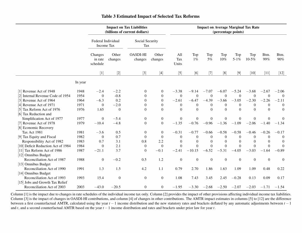
ologically motivated, are not included in zt . After the elimination of tax changes with delayed implementation, the
selection procedure yields a total of 15 tax reforms between 1946 and 2012 with significant and immediate impact on
personal tax liabilities. These reforms are listed in Table 3. The first four columns in Table 3 list the projected impact
on tax liabilities according to contemporaneous official sources. Columns [1] and [3] report the liability impact due
to changes in the rates and brackets of the federal individual income tax, and respectively, social security tax sched-
ules. Columns [2] and [4] report the liability impact of other provisions without direct impact on average marginal
tax rates, such as changes in deductions or coverage. Appendix A provides a description of the main provisions in
each of these reforms, as well as the sources of the liability impact estimates.
The precise impact of the selected tax reforms in zt is measured by scoring the AMTR impact of the legislative
change relative to pre-existing law. The scoring proceeds in a similar way as the calculation of the statutory compo-
nent of annual changes in AMTRs shown in Figure 4. However, instead of comparing to the previous year AMTR,
now the change is measured relative to the tax code that would have prevailed under prior law, i.e. in the absence of
the legislative change. More precisely, the estimated impact in year t of a given selected tax reform is the difference
between a first counterfactual tax rate, calculated using the year t− 1 income distribution and the current law rates
and brackets deflated by any automatic adjustments between t−1 and t, and a second counterfactual tax rate based
on the year t−1 income distribution and the prior law rates and brackets. The latter are obtained from official gov-
ernment publications sourced in appendix A. After scoring the tax reforms in this manner, eight out of the selected
15 tax reforms lead to a measurable change in AMTRs. These scores are shown in columns [5] to [12] in Table 3 and
reflect key provisions of many of the more important reforms, such as the tax cuts of 1948 and 1964, the Tax Reform
Act of 1986, the Bush-Clinton tax increases, as well as the acceleration in 2003 of earlier tax cuts. The time series
zt for exogenous unanticipated changes in the aggregate AMTR are the scores in the years of the tax reforms shown
in column [5] of Table 3, and zeros in all other years. Similarly, the time series for AMTR changes for the income
subgroups consists of the scores in the corresponding columns of Table 3 in reform years, and zero in all other years.
Several features of the time series zt for unanticipated AMTR changes merit further discussion. First, the num-
ber of observations is small. Of the fifteen reforms listed in Table 3, eight include direct changes to the basic income
tax rate schedules. The other seven selected reforms contain only provisions altering tax credits, deductions or cov-
19
erage, which affect tax liabilities but do not have any direct AMTR impact, or at least not one that is easily picked
up by the static scoring method. Appendix B.2 performs an analysis with an alternative instrument based on the tax
liability impact of all 15 reforms, and also verifies the sensitivity to the inclusion of particular reforms such as those
in the 1980s.
What is important is that the eight benchmark reforms still capture a large amount of variation in marginal tax
rates. Virtually all of this variation stems from federal income tax changes. Most changes to social security rates are
excluded because they fund benefit expansions and/or have long implementation lags. With only one minor excep-
tion, the reforms change AMTRs in the same direction for all income groups, but there is also some heterogeneity
across reforms in the relationship between income and the size of the change. In particular, the tax changes are
usually much larger for higher income taxpayers. There are six cuts in tax rates, three under Democratic and three
under Republican presidents.21 There are two tax increases, one under a Democratic and the other under a Republi-
can presidency. There is therefore no obvious relation with presidential party affiliation. Reforms lowering income
tax rates are generally more frequent, which is not surprising given the lack of indexation in the tax code. Finally,
the often lengthy political and legislative processes preceding tax reforms mean that the eventual marginal tax rate
changes were certainly to some extent anticipated prior to their enactment. This fact does not violate the identifying
assumptions since only contemporaneous exogeneity, but not lag exogeneity, with respect to other macroeconomic
shocks is required. As long as there is sufficient randomness in the timing and/or size of the changes, zt remains a
useful measure that is correlated with the underlying surprise changes.
4.3.2 Model Specifications
In addition to the time series for log net-of-tax rates and log income levels described earlier, the baseline SVAR-IV
model includes the following set of control variables in Xt : Log real GDP per tax unit, the unemployment rate, the
log real stock market index, inflation and the federal funds rate. These variables generally capture business cycle
conditions, interactions with monetary policy, as well as the effects of bracket creep. The controls Xt further in-
cludes log real government spending per tax unit (purchases and net transfers) and the change in log real federal
government debt per tax unit. These variables are included to capture interactions with other current and past fiscal
21Although the 1948 reform was passed after a Truman veto.
20
policies, in particular since tax changes are often motivated by concerns about government deficits.22 Our baseline
SVAR-IV specification is a VAR(2) for the nine endogenous variables estimated using yearly data from 1946-2012.
We also include dummy variables for 1949 and 2008 as additional regressors. As mentioned earlier, the baseline
LP-IV specification uses exactly the same right-hand-side variables as the SVAR-IV specification, i.e. Wt includes
two lags of income, net-of tax rates, the variables in Xt , and the dummy variables. We do not interact the dummy
variables with the remaining controls, which implicitly assumes that the slope coefficients of the both the SVAR-IV
and the LP-IV model are stable across the sample.
Our choice of macroeconomic controls is motivated by pre-test results indicating that the (recent) history of these
variables, income and tax rates contain the most relevant information to isolate the unanticipated short run innova-
tions in tax rates and income. Based on these variables, the VAR model is for instance quite successful in capturing
many of the known pre-announced tax rate changes.23 Appendix B.2 verifies robustness to a variety of changes in
the baseline specification. First, we discuss the lag structure. Standard lag selection criteria recommend one to three
lags. However, inspection of the residuals indicates a minimum of two lags is required to eliminate evidence of
residual autocorrelation. We use two lags in our baseline specifications, but we note that the point estimator for the
short run ETI obtained under either the SVAR-IV or the LP-IV model with three lags is very similar (in both cases
the confidence interval is wider, but the ETI remains significant at the 5% level).
Second, we discuss our selection of dummy variables. The inclusion of the 1949 and 2008 dummies, both re-
cession years, is not innocuous for the SVAR-IV results, but has virtually no impact on the LP-IV results (see the
first panel of Figure B.3). The first and last few years in the sample are periods of relative macroeconomic turbu-
lence and unusual policy variation associated with the end of WWII and the 2007-2009 financial crisis. Rather than
dropping these periods from the sample, as is common practice, the dummy approach yields results that are more
stable across subsamples while preserving the major 1948 tax reform as a source of identifying variation.24 We note
22Appendix A provides precise variable definitions and sources.23Results are available on request.24Romer and Romer (2010) and Barro and Redlick (2011) report the sensitivity to inclusion of the 1948 tax reform and use samples
starting in 1950 for their main analysis. We found the results to be much more sensitive to a dummy for the 1949 recession than includingthe 1948 reform. See Appendix B.2 for more discussion. Mertens and Ravn (2013) also focus on the 1950-2006 sample. Saez (2004) andSaez et al. (2012) use data for 1960-2000 and 1960-2006 respectively. Our choice of including dummy variables only allows for ‘breaks’in the model intercept. A more general specification would allow also for breaks in the slope parameters by interacting the dummy variablewith each of the controls. This is, however, not feasible given the size of our sample.
21
that with or without dummies, both the SVAR-IV and LP-IV estimators remain statistically significant at the 5% level.
Finally, Appendix B.2 also discusses sensitivity to the sample choice and to alternative versions of zt . We note
that the estimated responses of log-income based on an SVAR-IV model for the 1950-2006 sample are almost iden-
tical to the results obtained in our benchmark specification. The LP-IV estimated over the same period generates
different estimates, but these are larger than the benchmark at every horizon beyond impact.
4.4 The Response of Aggregate Income to Marginal Tax Rates
4.4.1 Weak Instrument Concerns and Inference
Unfortunately, the requirement of contemporaneous exogeneity of the series for zt is not testable since there are no
overidentifying restrictions. The relevance of zt as proxies or instruments, on the other hand, is testable. Before
turning to the main estimation results, we present formal statistical tests of the conditions in (7) and (11). Verifying
these relevance assumptions is important to assess whether weak instrument problems may bias our conclusions.
In the LP-IV framework, the relevance condition in (11) is the standard one for linear IV models. In our base-
line LP-IV specification with aggregate income and net-of-tax rates, the value for the first-stage F (using a Newey
and West (1987) HAC-robust residual covariance matrix with 8 lags) is 229.25 for the Barro and Redlick (2011) net-
of-tax rate, and 62.24 for the Piketty and Saez (2003) net-of-tax rate. Both these values are well above the threshold
value of 10 proposed by Stock and Yogo (2005), as well as the more stringent cutoff suggested by Montiel-Olea
and Pflueger (2013), indicating that zt is a highly relevant instrument for marginal tax rates. Based on these results,
we follow the standard 2SLS inference procedures in the LP-IV model, with Newey and West (1987) HAC-robust
standard errors.
The SVAR-IV relevance condition in equation (7) is subtly different from the one in a traditional linear IV model,
and we follow the inference procedures proposed in Montiel-Olea, Stock and Watson (2017). The relevant F-statistic
in the SVAR-IV model, which is provided in Appendix B.1, is 11.09 for the Barro and Redlick (2011) net-of-tax rate,
and 8.90 for the Piketty and Saez (2003) net-of-tax rate. The former value exceeds the Stock and Yogo (2005) thresh-
22
old, while the latter is just below.25 Both values exceed the 5%-level critical value of 3.84 for the null hypothesis of
zero covariance between zt and innovations to the AMTR series. Based on these first-stage test results, we conduct
inference in the SVAR-IV model using standard Delta-method confidence intervals as suggested by Montiel-Olea et
al. (2017), with a Newey and West (1987) HAC-robust residual covariance matrix.
Appendix B.1 discusses a number of alternative inference procedures for both the SVAR-IV and LP-IV models,
including weak-IV robust and bootstrap methods. The results show that virtually all alternative intervals for the
SVAR-IV/LP-IV estimates are close to the standard confidence intervals reported in the next section, and none lead
to any substantively different conclusions.
4.4.2 Estimation Results
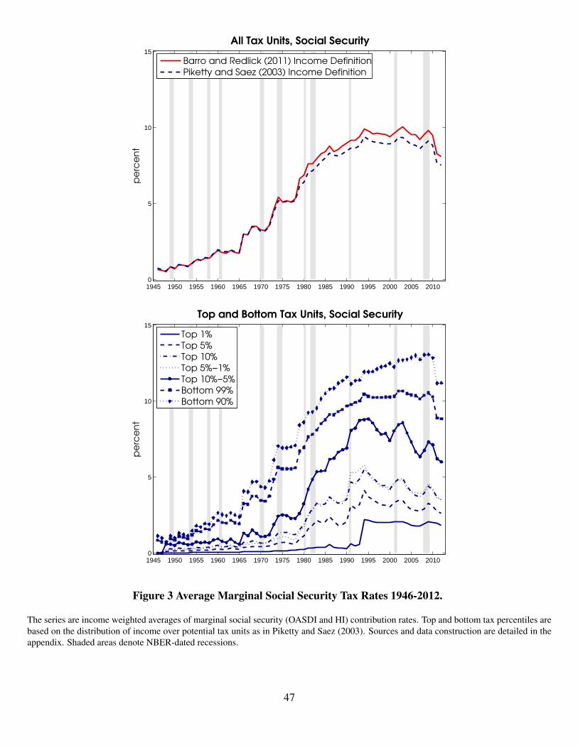
The first set of results is based on models that include aggregate reported income and the Barro and Redlick (2011)
aggregate net-of-tax rate. Figure 5 depicts the SVAR-IV impulse responses to a one percent increase in the aggregate
net-of-tax rate identified by imposing the conditions in (6) and (7) with non-zero observations in zt taking on the
values in column [5] of Table 3. Figure 6 shows the LP-IV impulse responses obtained using the same series as an
instrumental variable. All figures also display 68% and 95% confidence intervals. The income responses are on a
scale that is directly comparable to those of the time series regressions reported earlier in Table 2.
The SVAR-IV estimates in Figure 5 (top left panel) show that an unanticipated decrease in taxes has transitory
effects on the average marginal tax rate. The initial decrease in the tax rate persists almost perfectly in the following
year. From then onwards, the tax rate gradually reverts to the level expected prior to the shock. Although statutory
changes in federal tax rates are usually legislated as permanent, the estimates imply that in expectation policy shocks
are fully reversed by sunsets, subsequent reforms or bracket creep after five to six years. The estimated dynamic
adjustment of tax rates has two important implications for the interpretation of the results. First, since the tax rate
decrease persists almost perfectly in the following year, the one-period-after-the-shock income response provides a
plausible estimate of the short run ETI associated with a full year of lower tax rates. Second, the transitory nature of
changes in tax rates implies a potentially important role for timing and intertemporal substitution effects.
25We note that both values are substantially lower than those from the conventional first-stage F-test for linear IV models. This can arisebecause the validity of SVAR-IV and LP-IV inference relies on different high-level assumptions, see Appendix B.1 for more explanation.
23
Reported income per tax unit (bottom left panel) reacts positively to the unanticipated decrease in the AMTR. Income
rises on average by 0.71% in the year of the tax cut and by 1.37% in the following year. Both estimates are highly
statistically significant, and contrast sharply with the low and insignificant estimates for the aggregate elasticities in
the univariate regressions in the first column of panels A-C in Table 2. The income response remains significant at the
5% level for a full three years after the year of impact and peaks at almost 1.50% in the second. From then onwards,
incomes gradually decrease to levels expected prior to the shock, although the effects appear more persistent than the
decline in the AMTR. A cut in the marginal tax rate also leads to a significant increase in real GDP per capita (top
right panel) and a persistent and significant decline in the unemployment rate (bottom right panel). Real GDP rises
by 0.44% in the year of the cut, and by up to 0.78% two years after. The unemployment rate initially falls by 0.23
percentage points, and is 0.39 percentage points lower in the next year. Similar to the response of income reported
on tax returns, the output and unemployment responses are hump-shaped and more persistent than the change in tax
rates. Measured by the impulse response coefficient for the following year, the SVAR model yields a short run ETI
estimate for all tax units of 1.37, with a 95% confidence range of 0.80 to 1.94. Importantly, the responses of GDP
and unemployment indicate that the positive response of income reported to tax authorities coincides with important
real effects on economic activity.
Figure 6 shows the responses from the LP-IV regressions. For comparison, the figure also depicts the SVAR point
estimates as thinner lines. Because the LP-IV controls in Wt coincide exactly with the VAR right-hand-side vari-
ables, the impact responses in the SVAR-IV and LP-IV models are numerically identical for all outcome variables.
For horizons beyond zero, the estimates are different. However, the main conclusion from Figure 6 is that the LP-IV
responses nevertheless remain very close to those from the SVAR-IV. The income response is hump-shaped with a
similar peak of 1.54% at the same horizon, and is again highly statistically significant for three full years after the
year of impact. The LP-IV estimates also confirm the finding of important real effects on economic activity. Both the
GDP and unemployment responses are very similar in size and shape as those obtained in the SVAR-IV framework,
and they are statistically significant for the same horizon. Again, the tax rate decrease persists almost perfectly the
following year and then gradually reverts to the levels expected before the cut. The AMTR decrease is somewhat
more persistent when using local projections. Measured by the impulse response coefficient in the following year,
24
the LP-IV approach yields a short run ETI for all tax units of 1.19, with a 95% confidence range of 0.45 to 1.93.
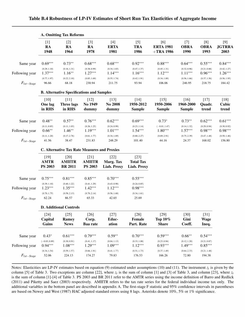
Appendix B.2 conducts a large number of checks to assess the robustness to various specification and sample
choices, and shows that the ETI estimates are not very sensitive to the inclusion of any particular tax act in the
proxy/instrument, including the larger 1948, 1964 or 1980s reforms. The inclusion of the dummies is more conse-
quential for the SVAR-IV estimates: the point estimate declines from 1.37 to 1.15 when the 2008 dummy is omitted
and to 0.96 when the 1949 dummy is dropped, although the estimates remain highly significant. The dummies are
less influential for the LP-IV estimates: the point estimate declines to 1.01 when the 2008 dummy is omitted, but
remains 1.19 when the 1949 dummy is dropped. Restricting the sample to 1950-2012, 1950-2006 or 1960-2000
raises the SVAR-based ETIs to 1.41, 1.50 and 1.40 respectively, and the LP-IV estimates to 1.54, 1.80 and 1.57,
respectively. In all these cases, the estimates remain highly significant. Using the AMTR series based on the Piketty
and Saez (2003) income concept, or the series that only captures the federal income taxes, also yields somewhat
larger ETI estimates. Appendix B.2 also documents similar results for two alternative series for zt based on official
estimates of the tax liability impact of the full set of 15 tax reforms. One source of concern is that the selected
tax reforms are systematically correlated with other policy changes. There is little historical or empirical evidence
of correlation with spending changes, see Romer and Romer (2010) or Mertens and Ravn (2013), but changes in
personal tax rates occasionally coincide with changes to corporate taxes in the same direction. An extended SVAR
model that controls for simultaneous changes in corporate taxes using the methodology of Mertens and Ravn (2013)
results in a similar ETI estimate of 1.35. Various additions to the set of control variables also have no major impact
and all SVAR/LP-IV point estimates remain similar in size and highly statistically significant.
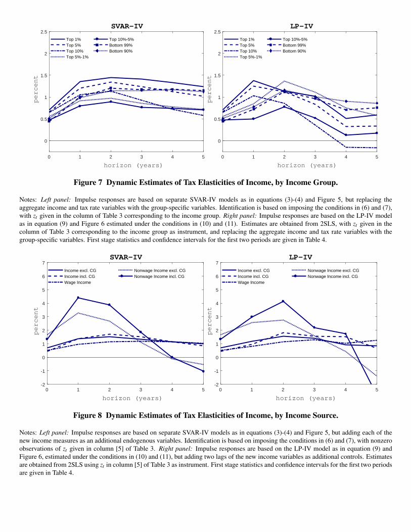
4.5 The Response to Marginal Tax Rates: Different Income Groups and Income Sources
According to the evidence in the previous sections, aggregate reported income and real GDP rise significantly follow-
ing persistent but transitory cuts in marginal tax rates, and unemployment falls. We now provide additional evidence
on the sensitivity of income to marginal tax rates by income groups and income source.
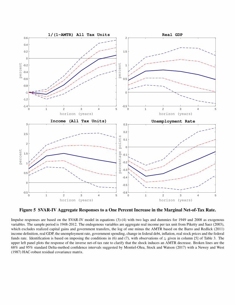
One way of assessing how ETIs differ across income groups is by estimating separate SVAR/LP-IV models for
each income group. The results are shown in Figure 7. The methodology for estimating the SVAR-IV responses
25
in the left panel of Figure 7 is the same as for the aggregate SVAR in the previous section, but the net-of-tax rate
and income series for all tax units are replaced with the corresponding series for each income group. The impulse
responses are identified by imposing the conditions in (6) and (7) using the corresponding income specific series
for zt based on the values in columns [6] to [12] in Table 3. The LP-IV estimates in the right panel are obtained
analogously using conditions (10) and (11). Both approaches identify ETIs associated with unanticipated changes
in group specific tax rates. Given the high correlation between tax rate changes implemented by the reforms, it is
important to keep in mind that the resulting estimates will also reflect effects from correlated tax rate changes for
other income groups. It is possible to identify the effects of income group specific tax shocks in isolation, and we
will pursue this avenue in Section 5.2 below.26
As can be seen in Figure 7, the estimated ETIs for the individual subgroups are positive at all horizons consid-
ered. The income responses are very similarly hump-shaped across income groups, peaking at values ranging from
around 0.8 for the top 10-5% bracket up to 1.5 for the top 1% bracket. The top 1% elasticities are consistently
the highest, but the elasticities are also large for all other income groups. Panel A in Table 4 reports the first two
SVAR-IV impulse responses coefficients for each income group, corresponding to the same and following year tax
elasticities, together with the confidence intervals. The top 1% elasticities are highly statistically significant, with a
following year estimate of 1.35. In sharp contrast to the results of the initial regressions in panels A-C of Table 2,
the SVAR-IV identified elasticities are also large and statistically significant at income levels outside of the top 1%.
The following year elasticities for the top 5-1% and top 10-5% are 0.91 and 0.79, while the bottom 99% and 90%
elasticities are 1.01 and 0.98, respectively.27 Panel A in Table 5 reports the LP-IV estimates. Just as for the aggregate
results, the ETIs for the bottom 90%-99% are slightly below those obtained from the SVAR-IV model, while those
for the top 1, 5 and 10% are about the same. The confidence intervals are wider, and the evidence for statistical
significance in the bottom groups is weaker. If the VAR model is indeed correctly specified, this is not surprising as
the LP-IV estimators are in that case less efficient. Both Tables 4 and 5 also report the F-statistics associated with
tests for the relevance assumptions, see Section 4.4.1. Because in a few cases the test results indicate possible weak
26Another strategy would be to study income shares or income differences between groups. Such a strategy, however, does not producemeaningful results if indeed the ETIs vary with income or if there are spill over effects, evidence for which we find in Section 5.2.
27Note that in Table 4 the ETIs by income group are all below and therefore seemingly inconsistent with the estimates for all tax units inthe first two columns. This, however, is because the distribution of the cuts across income groups, as well as the associated change in theAMTR for all tax units, will differ for every estimate. The implied decline in aggregate net-of-tax-rate is not equal to a one-percent decreasein the aggregate net-of-tax rate as in the first two columns of Table 4.
26
IV problems, Appendix B.1 provides alternative weak-instrument robust confidence intervals, without substantive
changes in the conclusions.
Taken together, the income-specific SVAR/LP-IV estimates contradict the conclusions in Saez (2004) or Saez et
al. (2012), and provide clear evidence for responses to tax rates that extend well beyond the highest incomes alone.
Consistent with the existing evidence, however, the estimated ETIs do remain larger for top incomes. Besides possi-
ble heterogeneity in real substitution behavior, one possibility is that the smaller tax rate changes for lower incomes
do not always incur sufficient utility losses to induce changes in behavior, see Chetty (2012). Another explanation
is that taxpayers with higher incomes have greater access to avoidance opportunities. If this is the case, than the
finding of more broad-based income responses is a further indication of real economic effects of tax changes. We
verified that our conclusions regarding the income group-specific ETI estimates are not sensitive to the inclusion of
any specific tax reforms in the zt variables.28
To gain further insight into the nature of the income response and the role of avoidance, Figure 8 shows the re-
sponses of different sources of income based on the data provided by Piketty and Saez (2003). The income measure
studied so far is real market income per tax unit excluding realized capital gains. Figure 8 shows the SVAR/LP-IV
responses of the wage and non-wage subcomponents of this measure. Non-wage income includes entrepreneurial
income (S-corporation, partnership and sole proprietorship profits), rents, dividends and interest, and accounts for
about 15% of reported income on average. The figure additionally shows the responses of broader measures of total
market and non-wage income that also include the realized capital gains reported on tax returns. Capital gains in the
US, on average around 5% of income, are taxed at a different rate, and the response of incomes that include capital
gains provides insight into the potential shifting of income between capital gains and other income as an avoidance
strategy. The SVAR-IV responses of the new income measures are obtained from separate SVAR models that are
the same as before, but add the new income variable of interest as an additional endogenous variable. The LP-IV
responses are obtained analogously, adding two lags of the additional income variable to the controls.
Figure 8 shows that both wage and non-wage sources of income react positively to the transitory but persistent
28One exception is the 1964 reform. When omitted, the bottom 99% and 90% ETIs are reduced to 0.71 and 0.51, respectively. The ETIestimates for all tax units and for top tax units, on the other hand, remain very similar. Results are available on request.
27
decrease in marginal tax rates. There are, however, some notable differences in the size and shape of the income
responses. Wage income, which reacts in a hump-shaped fashion with peaks of 1.19% (SVAR-IV) and 1.29% (LP-
IV) in the third full year after the year of impact, is less elastic than non-wage income (excluding capital gains),
which shows a peak increase of 3.29% in the following year using SVAR-IV, and of 2.76% one year later using
LP-IV. The rise in reported non-wage sources of income is more transitory than the reaction of wage income, which
is more delayed and persistent. Once marginal tax rates have returned to previous levels in the fifth year after the tax
cut (see Figure 5), the increase in non-wage income has dissipated entirely. The first column in Panels B and C of
Tables 4 and 5 reports the first two impulse responses coefficients for wage and non-wage income for all tax units.
The short-run aggregate wage and non-wage income responses are each highly statistically significant. Based on the
following year impact, the short run SVAR-IV elasticity of wage income is 0.94, which is significant at the 1% level.
The second-year SVAR-IV elasticity of non-wage income for all tax units is 3.29 and is also significant at the 1%
level. The corresponding LP-IV estimates are 0.81 and 2.93, respectively. The former is significant at the 10% level,
the latter at the 1% level.
The results in Figure 8 clearly show that reported aggregate non-wage income is especially responsive to taxes.
This may be due to real substitution effects, but potentially also to the fact that non-wage sources of income are
generally easier to time or conceal. To the extent it is less prone to avoidance effects, the significant rise in wage
income provides a stronger indication for a real economic response to tax rates. Nevertheless, certain taxpayers with
high incomes may still have considerable scope to shift labor income without any associated real change in income
generating activities, see e.g. Slemrod (1995, 1996). The remaining columns in Panels B and C of Tables 4 and 5
report the elasticities of wage and non-wage income for different income groups.29 As before, these are obtained
from separate SVAR/LP-IVs in which the series for all tax units are replaced with the corresponding series for each
income group. Interestingly, the elasticities of wage income are the largest for the top 1% and bottom 90% brack-
ets, and equal 0.96 and 0.90 in the SVAR-IV model, respectively. The sensitivity of bottom 90% wage income is
probably the least likely to be due to avoidance effects. Moreover, the statistically significant response of bottom
90% wage income is also consistent with the impact on unemployment in Figures 5 and 6. The following-year wage
29The wage share is decreasing in income, and is on average 44% for the Top 1%, 73% for the Top 5-1%, 86% for the Top 10-5%, and0.87% for the Bottom 90% (as a fraction of total market income including capital gains). The realized capital gains share is increasing inincome, and is on average 13% for the Top 1%, 5% for the Top 5-1%, 2% for the Top 10-5%, and 3% for the Bottom 90% (as a fraction oftotal market income including capital gains).
28
income SVAR-IV elasticities are considerably smaller for the brackets in between, with values for the top 5-1% and
top 10-5% of 0.14 and 0.63, respectively. Moreover, only the latter is statistically significant. For every income
group except the bottom 90%, the elasticity of non-wage income is much larger than the elasticity of wage income.
Interestingly, whereas wage income in the top 5-1% is essentially unresponsive, non-wage income in this group is
the most sensitive to taxes of all income groups. The short-run SVAR-IV elasticities of non-wage income are statis-
tically significant for all income groups within the top 5%, but insignificant outside of the top 5%. Once again, the
corresponding LP-IV estimates in Table 5 display very similar patterns. The confidence bands are generally wider,
and sometimes considerably so. In sum, there appears to be considerable heterogeneity in the type of income that
is sensitive to tax rates: exclusively wage income for the bottom 90%, and exclusively non-wage income for the top
5-1%. For the other income groups, it is a combination of both.
Finally, we discuss the role of income shifting between capital gains and other income. Figure 8 shows that to-
tal income and non-wage income both increase regardless of whether realized capital gains are included. The impact
responses become somewhat smaller, which provides some evidence for income shifting in the initial year of the tax
cut. However, in subsequent years the income responses become larger. Overall, including realized capital gains has
no major implications for the aggregate ETI estimates, which remain similar in size and highly statistically signif-
icant. Looking at individual income groups, however, there are more substantial differences that are suggestive of
income shifting by high income tax payers. Panels D and E of Tables 4 and 5 report the elasticities of total income
and non-wage income after including realized capital gains. For the top income groups, the inclusion of capital gains
reduces the ETI estimates, while the opposite is the case for the bottom 90% group. For the non-wage income elas-
ticities, similar results hold. Drawing firm conclusions is complicated by the fact that including the highly volatile
capital gains data often widens the confidence intervals considerably. Whereas the implications for aggregates appear
to be minor, including capital gains does flatten the ETI-income profile to the point where the ETIs become more
similar in size across income groups.
4.6 Discussion and Comparison with Earlier Evidence
The evidence for large ETIs and real economic responses to taxes is not an artifact of the use of VAR or LP techniques
widely used in macroeconomics. Instead, the main reason for the discrepancy with the time series evidence from
29
public finance is the IV step based on the selection of tax reforms by Romer and Romer (2009, 2010) to address the
endogeneity of tax policy. To make this unambiguous, panel D in Table 2 reports additional 2SLS estimates for the
original regressions of income growth on net-of-tax rate changes, but using only the Romer and Romer (2009, 2010)
selection of exogenous reforms as a instrument. The regressions, which are conceptually similar to those in Barro
and Redlick (2011), include exactly the same controls as in panels B and C of the same table, and also as in panel A
of Tables 4 and 5. The only difference with the previous regressions with controls in Table 2 is the instrument used
for changes in tax rates, which are now the same zt variables as in the SVAR/LP-IV models.
The 2SLS estimates in panel D of Table 2 confirm the large ETIs and establish the importance of accounting for
the endogeneity of tax policy. The estimates are, in fact, numerically identical to those from the LP-IV regressions
that use the levels of income and net-of-tax rates (panel Table A of Table 5). This equivalence is due to the fact that
the controls in the difference regressions are the same and include the levels of these variables. Comparing the vari-
ous panels in Tables 2, it is clear that each of the steps undertaken to control for confounding factors has the largest
effects for the lower income groups. For the bottom 90%, adding the predetermined variables raises the elasticity
from -0.52 to zero. Instrumenting with all statutory changes increases the ETI to 0.36, while instrumenting with the
exogenous tax rate changes brings the estimate up to 0.79. The same steps raise the top 1% elasticity by a smaller
amount, from 0.84 into the 1.30-1.40 range. The likely explanation is simply that the fraction of endogenous varia-
tion in tax rates is decreasing in income. Federal income tax policy interventions, in practice the dominant source of
useful identifying variation, explain a larger fraction of the tax rate variation at the top, see Table 1, and the same is
true for the exogenous measures in Table 3. Measured by the R2 coefficient, the zt series in columns [5] to [12] in
Table 3 explain 48% of the variation in all statutory changes for the top 1% but this decreases with income to 25% for
the bottom 90%. This indicates that cyclical and spending motivated policy changes are relatively more important
for lower incomes. Another contributing factor is that top marginal rates are much more insulated from bracket creep.
The size of the real economic responses estimated in the SVAR/LP-IV models is in a range consistent with many
previous findings in the macro and labor supply literatures. The GDP impact is roughly consistent with those in
Romer and Romer (2010) and Mertens and Ravn (2013) after rescaling from net-of-marginal rates to the average rate
measures used in these papers. The GDP response is about twice as large as the one found by Barro and Redlick
30
(2011), but this may be due to any of several differences in specification or because their estimate omits the same
year growth impact. Following Barro and Redlick (2011) and assuming a labor elasticity of output of one, the second
year GDP response suggests a value for the elasticity of aggregate hours of 0.78. Evaluated at the mean unemploy-
ment rate in the sample, the unemployment response suggest an extensive labor supply elasticity of 0.41. Taking
the difference yields an intensive labor supply elasticity of 0.37. Based on the summary of the quasi-experimental
evidence on the labor supply response to taxes, Chetty, Guren, Manoli and Weber (2013) consider values of 0.3 to
0.5 for the intensive margin and a value of 0.25 for the extensive margin as plausible. Our estimates are therefore
consistent with the labor supply evidence on the intensive margin elasticity, while the extensive elasticity is perhaps
moderately higher.
Taking a simple average of the SVAR/LP-IV estimates of the (following year) ETIs and each of the aggregate
AMTR measures yields a value of approximately 1.2 for all tax units. Since the estimates from numerous varia-
tions in specification reported in Appendix B.2 also average to a similar value, we take 1.2 as our baseline estimate
of the aggregate ETI. This number should be interpreted as the short-run macro elasticity associated with a per-
sistent but transitory change in average marginal tax rates that incorporates general equilibrium effects, as well as
intertemporal substitution effects. There obviously remains considerable uncertainty associated with the estimate, as
the confidence intervals still cover a relatively wide range of values. This is unavoidable given the sample size and
the extent of the postwar variation in marginal tax rates that can plausibly be classified as exogenous.
5 Additional Evidence for Real Responses to Marginal Tax Rates
The evidence for real economic effects of taxes remains open to several interpretations. Innovations in marginal tax
rates simultaneously induce changes in after tax incomes. The stimulative effects on income and employment may
therefore operate primarily through demand-side multiplier effects rather than direct effects on individual incentives.
The disaggregated ETI estimates show significant responses across income groups, but these incorporate the effects
of correlated tax rate changes among a large fraction of tax payers. It is therefore for instance not clear whether a tax
reform targeting top incomes alone would also have important real economic effects. This section presents additional
evidence for more specific counterfactual tax experiments to answer these questions.
31
5.1 Average versus Marginal Tax Rates
The Romer and Romer (2009, 2010) classification of postwar tax changes yields, after eliminating those with delayed
implementation, a total of fifteen plausible instances of tax policy ‘shocks’, see Table 3. The results so far are based
on a subset of eight of those instances corresponding to tax reforms with a direct impact on AMTRs through changes
in statutory rate schedules. The other seven tax policy changes had nontrivial effects on average tax rates but did not
alter the basic marginal rate schedules relative to prior law. Through modifications to tax credits, exemptions, deduc-
tions or coverage, the impact on average marginal tax rates of these policy changes is either zero or smaller and more
indirect. This section extends the SVAR-IV model to make use of these additional policy shocks for identification.
In addition to the series zt for shocks to the AMTR for all tax units used in Section 4.4, the identification strategy
relies on an additional time series for shocks to average tax rates. The approach exploits the historical variation in
the impact on average and marginal rates across tax reforms to isolate the effects of average and marginal tax rate
changes. The results provide insights into the importance of traditional multiplier effects for explaining the income
response to tax rate changes.
The SVAR specification is identical to Section 4.4, but now also includes the (log) average tax rate, or ATR, as
an additional endogenous variable, defined as total revenue and contributions as a ratio of the Piketty and Saez
(2003) measure of aggregate market income.30 Consider a vector containing the exogenous structural innovations
to the AMTR and the ATR, vτt = [vAMT R
t ,vAT Rt ]′ with E[vτ
t ] = 0. Let vot be the vector containing all other structural
shocks that affect the economy, which we now assume has a dimension equal to the number of variables less the two
tax policy shocks. Denoting the vector of marginal and average tax rate proxies by zt , the identifying assumptions
are:
E[ztvo′t ] = 0 . (12)
E[zt vτ′t ] = Φ , (13)
where Φ is an unknown nonsingular 2×2 matrix. As before, the first condition imposes contemporaneous exogene-
ity of the tax policy changes and is motivated by Romer and Romer (2009)’s narrative analysis. The second condition
30See appendix A for the precise definition.
32
states that the two measures of shocks to average and marginal rates (collected in zt) are contemporaneously corre-
lated with the true exogenous surprise innovations. Conditions (12) and (13) do not suffice to identify the dynamic
responses to AMTR and ATR exogenous shocks separately. However, as shown in Mertens and Ravn (2014), it is
possible to introduce an additional restriction on the responses of AMTR or ATR to identify the causal effects of
meaningful counterfactual tax experiments.
Using equations (3) and (4) and adding the ATR as an additional endogenous variable, we can express the tax
rates residuals uAMT Rt and uAT R
t in the VAR(2) of Section 4 as the bivariate system of simultaneous equations:
C
uAMT Rt
uAT Rt
= D
uincomet
uxt
+vAMT R
t
vAT Rt
, (14)
where C is a 2× 2 nonsingular matrix and D is 2× (dx + 1) matrix. The conditions (12) and (13) identify C′C and
C−1D, which is one condition too few to pin down C and D. However, there are two additional restrictions on the
AMTR and ATR responses that can be imposed consecutively and that are particularly meaningful.
Consider first the zero restriction C2,1 = 0. This upper triangular restriction on C yields the response to an unan-
ticipated counterfactual tax reform that, after controlling for current and lagged values of incomet , Xt , as well as for
lags of the tax rate variables, affects marginal rates but has no impact on statutory average tax rates. The associated
income response is therefore due to a change in marginal rates, since any direct effect of marginal tax rates on aver-
age tax rates in equation (14) is restricted to be zero on impact. The Tax Reform Act of 1986, with large marginal
rate reductions accompanied by various revenue enhancing provisions, is probably the closest historical equivalent
of this type of tax experiment. The upper triangular restriction C2,1 = 0 also identifies that response to an unexpected
change in the average tax rate, but allowing for impact on the statutory marginal rates.
Consider next the zero restriction C1,2 = 0. This lower triangular restriction on C corresponds to a counterfac-
tual tax reform that changes average tax rates but leaves statutory marginal rates unchanged. The associated income
response is likely to be predominantly generated by changes in disposable income and multiplier effects rather than
direct incentive effects, since at least on impact the statutory effect on marginal tax rates is imposed to be zero. Many
33
of the postwar tax policy interventions are of this type. The lower triangular restriction C1,2 = 0 also identifies that
response to an unexpected change in the marginal tax rate, but allowing for impact on the statutory average rate.
The additional proxy for average tax rates used for identification is the sum of columns [1] to [4] in Table 3 as a
ratio of total reported market income in the previous year, which yields an annual version of the quarterly narrative
measures of legislative changes in federal individual income and payroll taxes described in Mertens and Ravn (2013).
Similar to Romer and Romer (2010), innovations to average tax rates are measured by dividing the ex ante estimated
impact of the selected tax reforms on tax liabilities by (previous year) total income. The tax liability impact esti-
mates are obtained from official contemporaneous government sources such as the Joint Committee on Taxation or
the Congressional Budget Office. Appendix A provides the numbers and source documents, and Figure 9 presents
a scatter plot of the ATR and AMTR proxies. Unsurprisingly, the correlation between the average and marginal
tax rate impact of the tax reforms is high, and equals 0.90. In fact, the ATR changes from the 15 reforms can be
successfully used as an alternative relevant instrument for identifying impulse responses as in the previous Section.31
It is important to emphasize that the identification approach in this Section does not require both proxies to be uncor-
related, i.e. we do not impose that the matrix Φ in the condition (12) is diagonal. The identification scheme instead
exploits the variation in the ATR/AMTR impacts across the reforms, as well as the presence of reforms without direct
adjustments to the rate schedule (labeled as ‘without AMTR impact’). The regression line in Figure 9 is steeper than
the 45 degree line, which means that tax reforms making adjustments to the rate schedule (labeled as ‘with AMTR
impact’) typically induce larger changes in AMTRs than in ATRs. As mentioned before, the Tax Reform Act of 1986
is the most notable case of a reform with a large AMTR impact relative to the ATR impact.
Figure 10 depicts the dynamic responses to the counterfactual tax experiments, together with 68% and 95% Delta-
method confidence bands. For a clear comparison, Panel A first reports the case of a marginal tax rate shock that
does allow for impact on the statutory average tax rate (C1,2 = 0). Panel A establishes that including the average
tax rate in the VAR system, and using all fifteen exogenous reforms listed in Table 3, does not substantively alter
the earlier results. The income response to an increase in the net-of-tax rate of one percent is very similar in size to
Figure 5 and remains significant. Including the exogenous reforms without direct marginal rate provisions does not
lead to tighter estimates and, partly because of the larger system, the confidence bands are slightly wider than in the
31Columns [23] in Tables B.3 and B.4 of the Appendix show this yields very similar ETI estimates.
34
benchmark model. Not surprisingly, the average tax rate declines following a marginal rate cut.
Panel B in Figure 10 depicts the response to a marginal tax rate cut of the same size but now without any statu-
tory change in the average tax rate (C2,1 = 0). The associated response of income is very similar to Panel A and
the benchmark estimates, and is highly significant. The average tax rate still declines as a result of the estimated
net feedback from incomes and the variables in Xt , but the decline is much smaller and, in contrast to Panel A, not
statistically significant.
Finally, Panel C shows the response to a one percent average tax rate cut imposing no statutory impact on the AMTR
(C1,2 = 0). Even after allowing for indirect endogenous feedback, the response of the AMTR remains close to zero
throughout. The main finding is that, in sharp contrast to the results for marginal tax rate changes after controlling
for average tax rates, there is no evidence that income responds strongly to average tax rate changes once marginal
rate changes are controlled for. The point estimates are in fact slightly negative, although they are not statistically
significant at any horizon.
The findings in panel B and C of Figure 10 indicate that the large tax elasticities of income are not explained by
strong multiplier effects due to changes in after tax incomes. The results are instead much more consistent with
theoretical models that include direct incentive effects and forward looking substitution behavior. Based on a com-
parison of the regression coefficients on AMTR changes and the Romer and Romer (2009, 2010) series, Barro and
Redlick (2011) arrive at the same conclusion. The methodology above, which is the same as used by Mertens and
Ravn (2013) to separate the impacts of personal and corporate taxes, is in principle better suited for isolating the
causal effects of average and marginal tax rates. The results in Figure 10 also reveal that it is the subset of Romer
and Romer (2009) reforms with direct AMTR impact that is responsible for the finding of real economic effects of
tax policy shocks in the macro studies. Another implication is that measures of marginal tax rates are more relevant
and informative indicators of tax policy than the average tax rate measures that are more frequently used in macroe-
conometric studies. In terms of policy implications, an important qualification is, however, in order. Because many
lower income households face no federal income tax liabilities, the results may not be that informative about policies
that more strongly affect disposable incomes of those lower in the income distribution. Nonetheless, the results in
35
Figure 10 clearly emphasize the importance of marginal tax rates in explaining the evidence for the real economic
effects of tax reforms.
5.2 The Effects of Cutting Top or Bottom Marginal Tax Rates
Many of the postwar tax reforms have made particularly large changes in top marginal tax rates, and these changes
also account for an important fraction of the AMTR changes for all tax units. This section exploits the idiosyncratic
variation in tax rates for different income groups to estimate the effects of hypothetical tax reforms that only alters
marginal tax rates for a subgroup of taxpayers. The associated responses thus differ from those reported in Section
4.5, which did not control for simultaneous tax changes outside of the own income group. Isolating the causal effects
of more targeted marginal rate changes is potentially informative about general equilibrium and spill-over effects. It
is for instance less likely that top marginal rate changes directly generate a large demand stimulus. Focusing on top
rate changes in isolation also fits into recent policy discussions on optimal tax rates at the top, see e.g. Diamond and
Saez (2011), and provides insight into possible explanations for the correlation between top marginal tax rates and
top 1% income shares documented by Piketty et al. (2014) for the US and other OECD countries.
The key empirical challenge is to control for simultaneous exogenous changes in tax rates across income groups,
while at the same time preserving all endogenous feedback that arises because of changes in relative incomes, bracket
creep, etc. We address this challenge in exactly the same fashion as in the previous section isolating the separate
effects of average and marginal tax rates. The results are derived from an SVAR-IV model identical to Section 4.4 but
with two modifications. First, the aggregate AMTR and income series are replaced with the corresponding separate
series for the top 1% and bottom 99%. Second, following Saez (2004) and Saez et al. (2012), we include linear and
quadratic time trends to capture longer run trends in income inequality.32 The identification strategy relies on the
joint use of the proxies for shocks to the top 1% and bottom 99% AMTRs given in columns [6] and [11] of Table 3.
32Appendix B.2 shows that including the same time trends in the SVAR/LP-IV model for aggregate income of Section 4.4 does not haveany important effects.
36
The conditions in (12) and (13) and an additional zero restriction identify the coefficients in
C
utop 1% AMT Rt
ubtm 99% AMT Rt
= D
utop 1% income
t
ubtm 99% incomet
uxt
+ vtop 1%
t
vbtm 99%t
(15)
where the ut’s denotes the tax rate and income residuals. Imposing the upper triangular restriction C2,1 = 0 identifies
the response to an unanticipated counterfactual tax reform for the top 1% without any statutory change in rates for
the bottom 99%. Imposing C1,2 = 0 identifies the response to a shock to bottom 99% rates without any statutory
change for the top 1%.
Figure 10 displays the dynamic response to a targeted one percent rise in the net-of-tax rate of the top 1%, as
well as the associated 68% and 95% confidence bands. The upper left panel shows that the top marginal rate shock
causes a persistent but transitory decrease in the top 1% tax rate. The increase is more persistent than in the case
of an aggregate tax shock, which not only appears consistent with postwar policy decisions regarding top rates but
may also partly reflects that bracket creep is less relevant at the top of the income distribution. The upper right panel
shows that, after allowing for endogenous feedback, the response of the bottom 99% AMTR remains close to zero at
all horizons. This justifies interpreting the results beyond the impact period as also originating exclusively with top
marginal rate changes.
The panels in the second row of Figure 11 provide the responses of average incomes of both groups. The left
panel in the first row shows that the targeted tax cut leads to a significant increase in top 1% incomes, which rises
by 1.51% on impact and by 1.57% in the following year, after which there is a gradual decline. The response is
significant at the 5% level on impact, as well as for the two subsequent years. The following-year response is similar
and even slightly larger than those estimated earlier in Section 4.5. The rise in top 1% incomes is, however, more
transitory than in Section 4.5, and also more transitory than the aggregate income response in Section 4.4. Short run
ETIs for top incomes as large as 1.5 are similar to those initially found by Lindsey (1987) and Feldstein (1995) for the
1980s reforms, which made the largest changes to top statutory rates. Romer and Romer (2014) also focus on top rate
changes and control for tax rate changes for lower income groups by focusing on the interwar period, during which
37
only households with the highest incomes effectively paid income taxes. In diff-in-diff regressions using thin slices
at the top of the income distribution, Romer and Romer (2014) find much smaller short run elasticities of around
0.2. Whether this is due to differences between the pre- and postwar federal tax codes, the diff-in-diff strategy, the
persistence of the tax rate changes, data quality, or other factors is not clear.
According to the right panel in the second row of Figure 11, a cut in top rates has a positive effect on lower in-
comes. Average incomes of the bottom 99% rise by 0.23% on impact and by up to 0.44% in the following year.
The positive spill over effect is significant at the 5% level in the first and second year after the year of the tax cut.
Nonetheless, the top marginal rate cut unambiguously leads to greater inequality in pre-tax incomes. The results
are therefore consistent with the correlation between top statutory rates and top income shares observed in the US
and internationally. Piketty, Saez and Stantcheva (2014) propose a causal explanation for this correlation beyond
classical incentive or avoidance effects: lower top marginal tax rates lead to more aggressive rent-seeking efforts by
agents with the highest incomes. Avoidance or rent-seeking channels alone would imply zero or negative spill overs
from a top rate cut onto incomes outside the top. The positive impact on lower incomes does not invalidate these
channels, but suggests a dominant role for classical incentive effects. At least at this level of aggregation, the finding
of spill over effects also raises concerns with the interpretation of ETI estimates obtained using income shares or
income differences.
The bottom row of Figure 11 presents the response of GDP and the unemployment rate. The cut in the top 1%
AMTR leads to an increase in real GDP of 0.26% on impact and of 0.30% in the following year. Although the rise
in GDP is only marginally statistically significant, it nonetheless suggests that the positive top income response does
not result exclusively from avoidance or rent-seeking behavior. The finding that a top marginal rate cut leads to
increases in aggregate economic activity is corroborated by the unemployment response in the bottom right panel of
Figure 11, which shows that the unemployment rate is persistently lower by up to 17 basis points in the following
years. This decline is significant at the 5% level for the following year and the next. The positive spill over effects
on lower incomes may therefore be to an important extent driven by net job creation.
Figure 12 depicts the estimated effects of the reverse experiment of a targeted cut in marginal tax rates for the
38
bottom 99%. The right panel in the first row shows that the tax cut leads to a persistent but transitory decrease in the
bottom 99% AMTR. The top 1% AMTR is higher on impact and from the third period onwards, but its response is
very imprecisely estimated. The right panel in the second row of Figure 12 shows that bottom 99% incomes respond
positively to the targeted tax cut, rising by up to 2.1% in the third and fourth year after impact. There is, however,
a sharp difference in timing compared to the top 1% income response to its own AMTR in Figure 11. Bottom 99%
incomes show approximately no response in the short run, but increase only from the second year after the tax cut
onwards. In contrast, the top 1% income response in Figure 11 is immediate and more transitory. The effect of a
bottom 99% tax cut on top 1% incomes is ambiguous, negative in the first two years and positive afterwards, and has
very wide confidence bands. The eventual increase in income is highly statistically significant for the bottom 99%,
but insignificant for the top 1%. The impact decrease in top 1% incomes is marginally significant at the 5% level.
Finally, the bottom row of Figure 12 shows the response of GDP and the unemployment rate after a targeted tax
cut for taxpayers outside of the top 1%. The cut in bottom 99% tax rates leads to an increase in real GDP of up to
1.63% in the third year after impact, while the unemployment rate declines by up to 0.53 percentage points in the
same period. The timing of these responses is similar to the reaction of bottom 99% incomes, and shows a substantial
delay relative to the more immediate real effects estimated for a top 1% tax cut in Figure 12. Unsurprisingly, the
aggregate GDP and unemployment responses to a one percent cut in the net-of-tax rate for the bottom 99% are much
larger than to a narrower cut for only the top 1%. They are also considerably larger than to a one percent cut in the
net-of-tax rate for all tax units, see Figure 5, which reflects the larger and more idiosyncratic variability in top tax
rates in the postwar period. The difference in timing suggest that are important differences in the transmission mech-
anisms of cuts in top or bottom tax rates. As documented above, the typical unanticipated US tax reform changes
the entire rate schedule in the same direction. The real economic effects appear to be mostly driven by responses to
changes in top rates in the short run, while the effects of broader changes occur with a delay of several years. The
delayed response may also help explain why reactions to tax rates of incomes outside of the top have been harder to
detect empirically.
39
6 Concluding Remarks
Using a narrative identification strategy to obtain measures of exogenous variation in marginal tax rates, this study
finds significant and broad based effects on reported income. This is consistent with recent macro studies detecting
substantial effects of tax changes on real economic variables in the US and other countries using similar identifica-
tion approaches. However, it conflicts with existing evidence in the public finance literature that uses aggregate time
series constructed from tax returns data. We show that the difference can be explained by the efforts to resolve the en-
dogeneity of marginal tax rates due to tax policy being responsive to spending and the business cycle, bracket creep,
anticipation effects, etc. One may always question whether these efforts truly circumvent all endogeneity problems.
However, this paper demonstrates the important consequences of taking elementary steps to mitigate the influence of
confounding factors. As in any time series study, it is necessary to assume that the economic environment at some
level is stable across the sample. It is therefore always risky to draw strong conclusions about the impact of particular
historical or contemplated future tax reforms. With these caveats in mind, our findings are relevant for assessing the
role of income taxation for macroeconomic stabilization and the impact of austerity programs, for understanding the
empirical relationship between income taxes and inequality, and for optimal tax policy. The results also add more
indirectly to the growing evidence that hours and employment decisions are influenced by taxes, see e.g. Blundell,
Duncan and Meghir (1998), Keane (2011), Chetty (2012) and Chetty et al. (2013).
There are several ways for future research to verify and extend the analysis. The identification of exogenous variation
in marginal tax rates ultimately relies on a limited number of postwar tax reforms in the US. Tax returns data and
narrative datasets become increasingly available for other countries, e.g. Piketty et al. (2014), Cloyne (2013), Hayo
and Uhl (2014) and Leigh et al. (2014), which allows for replication of the results. Second, measuring the long run
effects of marginal tax rate changes in US data alone is extremely challenging. However, separating the effects of
temporary and permanent tax changes at least for top incomes may be feasible by incorporating prewar data. Third,
the empirical models in this paper are linear. There may be important nonlinearities in the relationship between
marginal tax rates and economic activity, both in the short and long run, see Auerbach and Gorodnichenko (2012)
or Jaimovich and Rebelo (2014). Finally, the results in this paper are based on reduced form models and should be
combined with realistic structural models to gain greater insight into the tax transmission mechanism. We leave these
and other extensions for future work.
40
References
Anderson, T. W., and H. Rubin, 1949, “Estimation of the Parameters of a Single Equation in a Complete Systemof Stochastic Equations”, Annals of Mathematical Statistics 20, pp. 46-63.
Auerbach, Alan J. and Yuriy Gorodnichenko, 2012, “Measuring the Output Responses to Fiscal Policy”, AmericanEconomic Journal: Economic Policy Vol. 4(2), pp. 1–27.
Auten, Gerald and Robert Carroll, 1995, “Behavior of the Affluent and the 1986 Tax Reform Act”, Proceedingsof the Annual Conference on Taxation Held under the Auspices of the National Tax Association-Tax Institute ofAmerica Vol. 87, pp. 70–76.
Auten, Gerald and Robert Carroll, 1999, “The Effect Of Income Taxes On Household Income”, Review of Eco-nomics and Statistics Vol. 81(4), pp. 681–693.
Badel, Alejandro and Mark Huggett, 2015, “The Sufficient Statistic Approach: Predicting the Top of the LafferCurve”, manuscript, Georgetown University.
Barro, Robert J. and Charles J. Redlick, 2011, “The Macroeconomic Effects of Government Purchases andTaxes”, Quarterly Journal of Economics Vol. 126(1), pp. 51–102.
Barro, Robert J., and Chaipat Sahasakul, 1983, “Measuring the Average Marginal Tax Rate from the IndividualIncome Tax”, Journal of Business Vol. 56(4), pp. 419–452.
Barro, Robert J., and Chaipat Sahasakul, 1986, “Average Marginal Tax Rates from Social Security and the Indi-vidual Income Tax”, Journal of Business Vol. 59(4), pp. 555–566.
Blundell, Richard, Alan Duncan and Costas Meghir, 1998, “Estimating Labor Supply Responses Using TaxReforms”, Econometrica, Vol. 66 (4), pp. 827–861.
Blundell, Richard, Monica Costa Dias, Costas Meghir and Jonathan M. Shaw, 2013, “Female Labor Supply,Human Capital and Welfare Reform”, NBER Working Paper No. 19007.
Caplan, Benjamin, 1956, “A Case Study: The 1948-1949 Recession”, in: “Policies to Combat Depression”, Na-tional Bureau of Economic Research, pp. 27–58.
Carroll, Robert, 1998, “Do Taxpayers Really Respond to Changes in Tax Rates: Evidence from the 1993 Tax Act”,U.S. Department of the Treasury Working Paper 79.
Chetty, Raj, 2009, “Is the Taxable Income Elasticity Sufficient to Calculate Deadweight Loss? The Implications ofEvasion and Avoidance”, American Economic Journal: Economic Policy Vol. 1(2), pp. 31–52.
Chetty, Raj, 2012, “Bounds on Elasticities with Optimization Frictions Avoidance: A Synthesis of Micro and MacroEvidence on Labor Supply”, Econometrica Vol. 80(3), pp. 969-1018.
Chetty, Raj, Adam Guren, Day Manoli and Andrea Weber, 2013, “Does Indivisible Labor Explain the Differencebetween Micro and Macro Elasticities? A Meta-Analysis of Extensive Margin Elasticities”, NBER Macroeco-nomics Annual, University of Chicago Press Vol. 27(1), pp. 1– 56.
Cloyne, James, 2013, “What Are the Effects of Tax Changes in the United Kingdom? New Evidence from aNarrative Evaluation”, American Economic Review Vol. 103(4), pp. 1507–1528.
Diamond, Peter and Emmanuel Saez, “The Case for a Progressive Tax: From Basic Research to Policy Recom-mendations”, Journal of Economic Perspectives Vol. 25(4), pp. 165–190.
Feenberg, Daniel R. and James M. Poterba, 1993, “Income Inequality and the Incomes of Very High-Income Taxpayers: Evidence from Tax Returns”, Tax Policy and the Economy 7, pp. 145–177.
Feldstein, Martin, 1969, “The Effects of Taxation on Risk Taking”, Journal of Political Economy Vol. 77(5), pp.755–764.
Feldstein, Martin, 1995, “The Effect of Marginal Tax Rates on Taxable Income: A Panel Study of the 1986 TaxReform Act”, Journal of Political Economy Vol. 103(3), pp. 551–572.
Feldstein, Martin, 1999, “Tax Avoidance and the Deadweight Loss of the Income Tax”, The Review of Economics
41
and Statistics Vol. 81(4), pp. 674–680.Giertz, Seth H., 2010, “The Elasticity of Taxable Income during the 1990s: New Estimates and Sensitivity Analy-
ses”, Southern Economic Journal Vol. 77(2), pp. 406–433.Goncalves, Silvia and Lutz Kilian, 2004, “Bootstrapping Autoregressions with Conditional Heteroskedasticity of
Unknown Form”, Journal of Econometrics Vol. 123(1), pp. 89–120.Goolsbee, Austen, 1999, “Evidence on the High-Income Laffer Curve from Six Decades of Tax Reform”, Brookings
Papers on Economic Activity No. 2Gruber, Jon and Emmanuel Saez, 2002, “The Elasticity of Taxable Income: Evidence and Implications”, Journal
of Public Economics Vol. 84, pp. 1-32.Hayo, Bernd and Matthias Uhl, 2014, “The Macroeconomic Effects of Legislated Tax Changes in Germany”,
Oxford Economic Papers Vol. 66(2), pp. 397–418.House,Christopher L. and Matthew D. Shapiro, 2006, “Phased-In Tax Cuts and Economic Activity”, American
Economic Review Vol. 96(5), pp. 1835–1849.Jaimovich, Nir and Sergio Rebelo, 2014, “Non-linear Effects of Taxation on Growth”, manuscript, USC Marshall
School of Business.Jentsch, Carsen and Kurt G. Lunsford, 2016, “Proxy SVARs: Asymptotic Theory, Bootstrap Inference, and the
Effects of Income Tax Changes in the United States”, Federal Reserve Bank of Cleveland Working Paper No.1619.
Jorda, Oscar, 2005, “Estimation and Inference of Impulse Responses by Local Projections”, American EconomicReview Vol. 95(1), pp. 161–182.
Jorda, Oscar, Schularick, Moritz, and Alan M Taylor, 2015, “Betting the house, Journal of International Eco-nomics Vol. 96, pp. S2–S18.
Lindsey, Lawrence B., 1987, “Individual Tax Payer Response to Tax Cuts 1982-1984: With Implications for theRevenue Maximizing Tax Rates”, Journal of Public Economic Vol. 33(2), pp. 173–206.
Keane, Michael P., 2011, “Labor Supply and Taxes: A Survey”, Journal of Economic Literature Vol. 49(4), pp.961-1075.
Keane, Michael P. and Richard Rogerson, 2012, “Micro and Macro Labor Supply Elasticities: A Reassessment ofConventional Wisdom”, Journal of Economic Literature Vol. 50(2), pp. 464-476.
Kueng, Lorenz, 2014, “Identifying the Household Consumption Response to Tax Expectations using Bond Prices”,NBER Working Paper No. 20437.
Leeper, Eric M., Todd B. Walker and Shu-Chun Susan Yang, 2013, “Foresight and Information Flows”, Econo-metrica Vol. 81(3), pp. 1115-1145.
Leigh, Daniel, Andrea Pescatori and Jaime Guajardo, 2014, “Expansionary Austerity New International Evi-dence”, Journal of the European Economic Association Vol. 12(4), pp. 949–968.
Lutkepohl, Helmut, 1990, “Asymptotic Distributions of Impulse Response Functions and Forecast Error VarianceDecompositions of Vector Autoregressive Models”, The Review of Economics and Statistics, pp. 116–125.
McGrattan, Ellen R., “The Macroeconomic Effects of Distortionary Taxation”, Quarterly Journal of EconomicsVol. 127(3), pp. 1515–1550.
Mertens, Karel and Morten Ravn, 2012, “Empirical Evidence on the Aggregate Effects of Anticipated and Unan-ticipated US Tax Policy Shocks”, American Economic Journal: Economic Policy Vol. 4(2), pp. 145–181.
Mertens, Karel and Morten Ravn, 2013, “The Dynamic Effects of Personal and Corporate Income Tax Changesin the United States”, American Economic Review Vol. 103(4), pp. 1212–1247.
Mertens, Karel and Morten Ravn, 2014, “A Reconciliation of SVAR and Narrative Estimates of Tax Multipliers”,Journal of Monetary Economics Vol. 68 supplement, pp. S1–S19.
Montiel Olea, Jose L., and Carolin Pflueger, 2013, “A robust test for weak instruments”, Journal of Business &Economic Statistics Vol. 31(3), pp. 358–369.
Montiel Olea, Jose L., James H. Stock and Mark W. Watson, 2017, “Inference in SVARs Identified with External
42
Instruments.”, Working Paper Columbia University.Newey, Whitney K. and Kenneth D. West, 1987, “A Simple, Positive Semi-definite, Heteroskedasticity and Auto-
correlation Consistent Covariance Matrix”, Econometrica 55(3), pp. 703-708.Parker, Jonathan A. and Annette Vissing-Jørgensen, “The Increase in Income Cyclicality of High-Income House-
holds and Its Relation to the Rise in Top Income Shares,” Brookings Papers on Economic Activity Vol. 41(2), pp.1-70.
Pechman, Joseph A., 1987, “Federal Tax Policy, Fifth Edition”, Brookings Institution, Washington DC.Piketty, Thomas and Emmanuel Saez, 2003, “Income Inequality in the United States, 1913-1998”, Quarterly
Journal of Economics Vol. 118(1), pp. 1–39.Piketty, Thomas and Emmanuel Saez, 2007, “Income Inequality in the United States, 1913-2002”, in Top Incomes
Over the Twentieth Century, A.B. Atkinson and T. Piketty eds., Oxford University Press, 2007.Piketty, Thomas, Emmanuel Saez and Stefanie Stantcheva, 2014, “Optimal taxation of Top Incomes: A Tale of
Three Elasticities”, American Economic Journal: Economic Policy Vol. 6(1), pp. 230–271.Ramey, Valerie A., 2011a, “Identifying Government Spending Shocks: It’s All in the Timing”, Quarterly Journal of
Economics Vol. 126(1), pp. 10–50.Ramey, Valerie A., 2011b, “Can Government Purchases Stimulate the Economy?”, Journal of Economic Literature
Vol. 49(3), pp. 673–85.Ramey, Valerie A., 2016, “Macroeconomic Shocks and Their Propagation”, Handbook of Macroeconomics, forth-
coming.Ramey, Valerie A. and Sarah Zubairy, 2017, Government Spending Multipliers in Good Times and in Bad: Evi-
dence from U.S. Historical Data, Journal of Political Economy, forthcoming.Romer, Christina D., and David H. Romer, 2009, “A Narrative Analysis of Postwar Tax Changes”, University of
California, Berkeley, manuscript.Romer, Christina D., and David H. Romer, 2010, “The Macroeconomic Effects of Tax Changes: Estimates Based
on a New Measure of Fiscal Shocks”, American Economic Review Vol. 100(3), pp. 763–801.Romer, Christina D., and David H. Romer, 2014, “The Incentive Effects of Marginal Tax Rates: Evidence from
the Interwar Era”, American Economic Journal: Economic Policy Vol. 6(3), pp. 242-281.Saez, Emmanuel, 2001, “Using Elasticities to Derive Optimal Income Tax Rates”, Review of Economic Studies
Vol. 68, pp. 205–229.Saez, Emmanuel, 2003, “The Effect of Marginal Tax Rates on Income: a Panel Study of Bracket Creep”, Journal of
Public Economics Vol. 87, pp. 1231–1258.Saez, Emmanuel, 2004, “Reported Incomes and Marginal Tax Rates, 1960-2000: Evidence and Policy Implica-
tions”, in: Tax Policy and the Economy Vol. 18, Editor J. Poterba, pp. 117–172.Saez, Emmanuel, Joel Slemrod and Seth. H. Giertz, 2012, “The Elasticity of Taxable Income with Respect to
Marginal Tax Rates: A Critical Review”, Journal of Economic Literature Vol. 50(1), pp. 3–50.Sammartino, Frank and David Weiner, 1997, “Recent Evidence on Taxpayers’ Response to the Rate Increases in
the 1990s”, National Tax Journal Vol. 50(3), pp. 683–705.Sims, Christopher, 1980, “Macroeconomics and Reality”, Econometrica Vol. 48(1), pp. 1–48.Shiller, Robert J., 2000, “Irrational Exuberance”, Princeton University Press.Slemrod, Joel, 1995, “Income Creation or Income Shifting? Behavioral Responses to the Tax Reform Act of 1986”,
American Economic Review Vol. 85(2), pp. 175–180.Slemrod, Joel, 1996, “High-Income Families and the Tax Changes of the 1980s: The Anatomy of Behavioral Re-
sponse” in: Empirical Foundations of Household Taxation, edited by Martin Feldstein and James M. Poterba,Chicago and London: University of Chicago Press, pp. 169–189.
Slemrod, Joel, 1998, “Methodological Issues in Measuring And Interpreting Taxable Income Elasticities”, NationalTax Journal 51(4), pp. 773–788.
Stock, James H. and Motohiro Yogo, 2005, “IV Regression, Identification and Inference for Econometric Models:
43
Essays in Honor of Thomas Rothenberg”, edited by D.W. Andrews and J.H. Stock, pp. 80–108.Stock, James H. and Mark W. Watson, 2008, “What’s New in Econometrics - Time Series”, NBER Summer
Institute, Lecture 7.Stock, James H. and Mark W. Watson, 2012, “Disentangling the Channels of the 2007-2009 Recession”, Brook-
ings Papers on Economic Activity Spring 2012, pp. 81–135.Stock, James H. and Mark W. Watson, 2017, “Identification and Estimation of Dynamic Causal Effects in Macroe-
conomics”, Working Paper Harvard University.Triest, Robert K., 1998, “Econometric Issues in Estimating the Behavioral Response to Taxation: A Nontechnical
Introduction”, National Tax Journal Vol. 51(4) pp. 761–772.Yang, Shu-Chun Susan, 2005, “Quantifying Tax Effects under Policy Foresight”, Journal of Monetary Economics
Figure 1 Average Marginal Tax Rates 1946-2012: Individual Income and Social Security.
The series are income weighted averages of marginal federal individual income tax rates and social security (OASDI and HI) contributionrates. Top and bottom tax percentiles are based on the distribution of income over potential tax units as in Piketty and Saez (2003). Sourcesand data construction are detailed in the appendix. Shaded areas denote NBER-dated recessions.
Figure 2 Average Marginal Individual Income Tax Rates 1946-2012.
The series are income weighted averages of marginal federal individual income tax rates. Top and bottom tax percentiles are based on thedistribution of income over potential tax units as in Piketty and Saez (2003). Sources and data construction are detailed in the appendix.Shaded areas denote NBER-dated recessions.
Figure 3 Average Marginal Social Security Tax Rates 1946-2012.
The series are income weighted averages of marginal social security (OASDI and HI) contribution rates. Top and bottom tax percentiles arebased on the distribution of income over potential tax units as in Piketty and Saez (2003). Sources and data construction are detailed in theappendix. Shaded areas denote NBER-dated recessions.
Figure 4 Estimates of the Impact of Statutory Changes on Average Marginal Tax Rates.
Observed annual change in the Barro and Redlick (2011) income concept AMTR for all tax units. The impact of statutory changes in year tis the difference between a counterfactual AMTR constructed using the year t−1 income distribution and year t rates and brackets deflatedby any automatic adjustments between t−1 and t, and the observed year t−1 average marginal tax rate.
0 1 2 3 4 5
horizon (years)
-1.4
-1.2
-1
-0.8
-0.6
-0.4
-0.2
0
0.2
0.4
0.6
percent
1/(1-AMTR) All Tax Units
0 1 2 3 4 5
horizon (years)
-0.5
0
0.5
1
1.5
2
percent
Real GDP
0 1 2 3 4 5
horizon (years)
-0.5
0
0.5
1
1.5
2
2.5
3
percent
Income (All Tax Units)
0 1 2 3 4 5
horizon (years)
-0.6
-0.5
-0.4
-0.3
-0.2
-0.1
0
0.1
0.2
0.3
percentage points
Unemployment Rate
Figure 5 SVAR-IV Aggregate Responses to a One Percent Increase in the Marginal Net-of-Tax Rate.
Impulse responses are based on the SVAR-IV model in equations (3)-(4) with two lags and dummies for 1949 and 2008 as exogenousvariables. The sample period is 1948-2012. The endogenous variables are aggregate real income per tax unit from Piketty and Saez (2003),which excludes realized capital gains and government transfers, the log of one minus the AMTR based on the Barro and Redlick (2011)income definition, real GDP, the unemployment rate, government spending, change in federal debt, inflation, real stock prices and the federalfunds rate. Identification is based on imposing the conditions in (6) and (7), with observations of zt given in column [5] of Table 3. Theupper left panel plots the response of the inverse net-of-tax rate to clarify that the shock induces an AMTR decrease. Broken lines are the68% and 95% standard Delta-method confidence intervals suggested by Montiel-Olea, Stock and Watson (2017) with a Newey and West(1987) HAC-robust residual covariance matrix.
0 1 2 3 4 5
horizon (years)
-1.4
-1.2
-1
-0.8
-0.6
-0.4
-0.2
0
0.2
0.4
percent
1/(1-AMTR) All Tax Units
LPIV
SVAR
0 1 2 3 4 5
horizon (years)
-0.5
0
0.5
1
1.5
2
percent
Real GDP
LPIV
SVAR
0 1 2 3 4 5
horizon (years)
-0.5
0
0.5
1
1.5
2
2.5
percent
Income (All Tax Units)
LPIV
SVAR
0 1 2 3 4 5
horizon (years)
-0.6
-0.5
-0.4
-0.3
-0.2
-0.1
0
0.1
0.2
0.3
percentage points
Unemployment Rate
LPIV
SVAR
Figure 6 LP-IV Aggregate Responses to a One Percent Increase in the Marginal Net-of-Tax Rate.
Impulse responses are based on the LP-IV regression in equation (9) estimated under assumptions (10)-(11). The control variables are twolags of each of the following variables: aggregate real income per tax unit from Piketty and Saez (2003), which excludes realized capitalgains and government transfers; the log of one minus the AMTR based on the Barro and Redlick (2011) income definition; real GDP; theunemployment rate; government spending; change in federal debt; inflation; real stock prices; and the federal funds rate. The regressionalso include dummies for 1949 and 2008. Estimates are obtained from 2SLS using zt in column [5] of Table 3 as instrument. The upper leftpanel plots the response of the inverse net-of-tax rate to clarify that the shock induces an AMTR decrease. Broken lines are 68% and 95%confidence bands based on Newey and West (1987) HAC-robust standard errors. The fine black line repeats the SVAR-IV estimates fromFigure 5 for comparison.
0 1 2 3 4 5
horizon (years)
0
0.5
1
1.5
2
2.5percent
SVAR-IV
Top 1%Top 5%Top 10%Top 5%-1%
Top 10%-5%Bottom 99%Bottom 90%
0 1 2 3 4 5
horizon (years)
0
0.5
1
1.5
2
2.5
percent
LP-IV
Top 1%Top 5%Top 10%Top 5%-1%
Top 10%-5%Bottom 99%Bottom 90%
Figure 7 Dynamic Estimates of Tax Elasticities of Income, by Income Group.
Notes: Left panel: Impulse responses are based on separate SVAR-IV models as in equations (3)-(4) and Figure 5, but replacing theaggregate income and tax rate variables with the group-specific variables. Identification is based on imposing the conditions in (6) and (7),with zt given in the column of Table 3 corresponding to the income group. Right panel: Impulse responses are based on the LP-IV modelas in equation (9) and Figure 6 estimated under the conditions in (10) and (11). Estimates are obtained from 2SLS, with zt given in thecolumn of Table 3 corresponding to the income group as instrument, and replacing the aggregate income and tax rate variables with thegroup-specific variables. First stage statistics and confidence intervals for the first two periods are given in Table 4.
0 1 2 3 4 5
horizon (years)
-2
-1
0
1
2
3
4
5
6
7
percent
SVAR-IV
Income excl. CGIncome incl. CGWage Income
Nonwage Income excl. CGNonwage Income incl. CG
0 1 2 3 4 5
horizon (years)
-2
-1
0
1
2
3
4
5
6
7
percent
LP-IV
Income excl. CGIncome incl. CGWage Income
Nonwage Income excl. CGNonwage Income incl. CG
Figure 8 Dynamic Estimates of Tax Elasticities of Income, by Income Source.
Notes: Left panel: Impulse responses are based on separate SVAR-IV models as in equations (3)-(4) and Figure 5, but adding each of thenew income measures as an additional endogenous variables. Identification is based on imposing the conditions in (6) and (7), with nonzeroobservations of zt given in column [5] of Table 3. Right panel: Impulse responses are based on the LP-IV model as in equation (9) andFigure 6, estimated under the conditions in (10) and (11), but adding two lags of the new income variables as additional controls. Estimatesare obtained from 2SLS using zt in column [5] of Table 3 as instrument. First stage statistics and confidence intervals for the first two periodsare given in Table 4.
-3.5 -3 -2.5 -2 -1.5 -1 -0.5 0 0.5 1 1.5
ATR proxy
-5
-4
-3
-2
-1
0
1
2
AMTR proxy
RA 1948
RA 1964
RA 1978
ERTA 1981
TRA 1986
OBRA 1990OBRA 1993
JGTRRA 2003
Correlation: 0.90
Reforms with AMTR impact
Reforms without AMTR impact
OLS regression line
45 degree line
Figure 9 Scatter Plot of the AMTR and ATR Proxies
Notes: The AMTR proxy is given in column [5] of Table 3, and the ATR proxy is the sum of columns [1] to [4] in Table 3, divided by totalreported market income from Piketty and Saez (2003) in the previous year.
A. Cut in Marginal Tax Rate Allowing Impact on Statutory Average Tax Rate
0 1 2 3 4 5
horizon (years)
-1
0
1
perc
ent
1/(1-AMTR) All Tax Units
0 1 2 3 4 5
horizon (years)
-2
0
2
perc
ent
Average Tax Rate
0 1 2 3 4 5
horizon (years)
-1
0
1
2
3
4
percent
Income (All Tax Units)
B. Cut in Marginal Tax Rate Without Impact on Statutory Average Tax Rate
0 1 2 3 4 5
horizon (years)
-1
0
1
perc
ent
1/(1-AMTR) All Tax Units
0 1 2 3 4 5
horizon (years)
-2
0
2
perc
ent
Average Tax Rate
0 1 2 3 4 5
horizon (years)
-1
0
1
2
3
4
percent
Income (All Tax Units)
C. Cut in Average Tax Rate Without Impact on Statutory Marginal Tax Rate
0 1 2 3 4 5
horizon (years)
-1
0
1
perc
ent
1/(1-AMTR) All Tax Units
0 1 2 3 4 5
horizon (years)
-1
0
1
perc
ent
Average Tax Rate
0 1 2 3 4 5
horizon (years)
-1.5
-1
-0.5
0
0.5
1
percent
Income (All Tax Units)
Figure 10 SVAR-IV Dynamic Responses to Shocks to Average and Marginal Rates.
Panels A and B show dynamic responses to a one percent increase in the marginal net-of-tax rate. Panel C shows the response to a onepercent decline in the average tax rate. Estimates are from SVAR-IV model as in Figure 5 but with the log average tax rate as an additionalendogenous variable. Identification is based on imposing the conditions in (12) and (13). Panels A and C use the restriction C1,2 = 0, andPanel B uses the restriction C2,1 = 0. The proxy for marginal tax rates is given in column [5] of Table 3, the proxy for average tax rates is thesum of columns [1] to [4] in Table 3 , divided by total reported market income from Piketty and Saez (2003) in the previous year. Brokenlines are 68% and 95% confidence bands based on the Delta method suggested by Montiel-Olea, Stock and Watson (2017), with a Neweyand West (1987) HAC-robust residual covariance matrix.
0 1 2 3 4 5
horizon (years)
-2
-1.5
-1
-0.5
0
0.5
1
percent
1/(1-AMTR) Top 1% Tax Units
0 1 2 3 4 5
horizon (years)
-0.4
-0.3
-0.2
-0.1
0
0.1
0.2
0.3
percent
1/(1-AMTR) Btm 99% Tax Units
0 1 2 3 4 5
horizon (years)
-1
-0.5
0
0.5
1
1.5
2
2.5
percent
Income Top 1% Tax Units
0 1 2 3 4 5
horizon (years)
-0.8
-0.6
-0.4
-0.2
0
0.2
0.4
0.6
0.8
percent
Income Btm 99% Tax Units
0 1 2 3 4 5
horizon (years)
-0.6
-0.4
-0.2
0
0.2
0.4
0.6
percent
Real GDP
0 1 2 3 4 5
horizon (years)
-0.3
-0.25
-0.2
-0.15
-0.1
-0.05
0
0.05
0.1
0.15
0.2
percentage points
Unemployment Rate
Figure 11 SVAR-IV Responses to a One Percent Increase in the Top 1% Marginal Net-of-Tax Rate.
Estimates are from a single SVAR-IV model as in Figure 5, but replacing aggregate net-of-tax rates and income with the series for the top 1%and bottom 99%, and adding a quadratic time trend. Identification is based on imposing the conditions in (12) and (13) and the restrictionC2,1 = 0. The proxies for marginal tax rates are given in columns [6] and [11] of Table 3. Broken lines are 68% and 95% confidence bandsbased on the Delta method suggested by Montiel-Olea, Stock and Watson (2017), with a Newey and West (1987) HAC-robust residualcovariance matrix.
0 1 2 3 4 5
horizon (years)
-3
-2
-1
0
1
2
3
4
5
percent
1/(1-AMTR) Top 1% Tax Units
0 1 2 3 4 5
horizon (years)
-2
-1.5
-1
-0.5
0
0.5
1
percent
1/(1-AMTR) Btm 99% Tax Units
0 1 2 3 4 5
horizon (years)
-10
-5
0
5
percent
Income Top 1% Tax Units
0 1 2 3 4 5
horizon (years)
-1.5
-1
-0.5
0
0.5
1
1.5
2
2.5
3
3.5
percent
Income Btm 99% Tax Units
0 1 2 3 4 5
horizon (years)
-1
-0.5
0
0.5
1
1.5
2
2.5
percent
Real GDP
0 1 2 3 4 5
horizon (years)
-0.8
-0.6
-0.4
-0.2
0
0.2
0.4
0.6
percentage points
Unemployment Rate
Figure 12 SVAR-IV Responses to a One Percent Increase in the Bottom 99% Marginal Net-of-Tax Rate.
Estimates are from a single SVAR-IV model as in Figure 5, but replacing aggregate net-of-tax rates and income with the series for the top 1%and bottom 99%, and adding a quadratic time trend. Identification is based on imposing the conditions in (12) and (13) and the restrictionC1,2 = 0. The proxies for marginal tax rates are given in columns [6] and [11] of Table 3. Broken lines are 68% and 95% confidence bandsbased on the Delta method suggested by Montiel-Olea, Stock and Watson (2017), with a Newey and West (1987) HAC-robust residualcovariance matrix.
Table 1 Average Marginal Tax Rates 1946-2012: Descriptive Statistics
AMTR×100 ∆ ln(1−AMTR)×100
% of total variation due toMean St. Dev. St. Dev. Correlation with statutory changes in
Notes: Descriptive statistics for combined federal income and social security tax rates. AMTR is the tax rate in percent and ∆ ln(1−AMTR)is the annual log change in the net-of-tax rate. Rows [1]-[2] are national averages using Barro and Redlick (2011), resp. Piketty and Saez(2003) income concepts. Rows [3] to [9] are averages within the specified brackets using the income measures of Piketty and Saez (2003).The last three columns report the R2 coefficient of regressions of ∆ ln(1−AMTR) on the estimated impact of statutory changes to incometaxes, social security taxes, or both, on the overall tax rates of the specified income bracket.
Table 2 Univariate Regressions of Income on Net-of-Tax Rates, Sample: 1948-2012
All Tax Units Top 1% Top 5% Top 10% Top 5-1% Top 10-5% Btm. 99% Btm. 90%BR 2011 PS 2003
A. Ordinary Least Squares, Sample: 1947-2012
Same year −0.23 −0.21 0.55∗∗ 0.37 0.28 0.02 −0.00 −0.35∗∗ −0.49∗∗∗
Notes: Same year estimates are based on regressing ∆ ln(income jt ) on ∆ ln(1−AMT R j
t ) and following year estimates are based on regressingln(income j
t+1)− ln(income jt−1) on ∆ ln(1−AMT R j
t ) for every income group j, see equations (1) and (2). The regressions in Panels B, Cand D include two lags of ln(income j
t ) and ln(1−AMT R jt ) as well as two lags of GDP, unemployment rate, government spending, change
in federal debt, inflation, real stock prices and the federal funds rate and dummies for 1949 and 2008. Results in the first column are basedon the AMTR series for all tax units using the income definition of Barro and Redlick (2011). The other series are based on the incomedefinition of Piketty and Saez (2003). Panel C uses all statutory tax changes as the instrumental variable. Panel D uses the narrativelyidentified tax changes as instruments, with the non-zero observations listed in columns [5] to [12] in Table 3. The first-stage F statistic and95% confidence intervals in parentheses are based on Newey and West (1987) HAC adjusted standard errors using 8 lags. Asterisks denote10%, 5% or 1% significance.
Table 3 Estimated Impact of Selected Tax Reforms
Impact on Tax Liabilities Impact on Average Marginal Tax Rate(billions of current dollars) (percentage points)
Federal Individual Social SecurityIncome Tax Tax
Changes Other OASDI-HI Other All Top Top Top Top Top Btm. Btm.in rate changes changes changes Tax 1% 5% 10% 5-1% 10-5% 99% 90%
Column [1] is the impact due to changes in rate schedules of the individual income tax only. Column [2] provides the impact of other provisions affecting individual income tax liabilities.Column [3] is the impact of changes in OASDI-HI contributions, and column [4] of changes in other contributions. The AMTR impact estimates in columns [5] to [12] are the differencebetween a first counterfactual AMTR, calculated using the year t−1 income distribution and the new statutory rates and brackets deflated by any automatic adjustments between t−1and t, and a second counterfactual AMTR based on the year t−1 income distribution and rates and brackets under prior law for year t.
Table 4 SVAR-IV Estimates of Short Run Tax Elasticities, Sample: 1948-2012
All Tax Units Top 1% Top 5% Top 10% Top 5-1% Top 10-5% Btm. 99% Btm. 90%BR 2011 PS 2003
A.Total Market Income (excluding Capital Gains)
Same year 0.71∗∗∗ 0.75∗∗∗ 0.71∗∗∗ 0.66∗∗∗ 0.65∗∗∗ 0.56∗∗∗ 0.47∗∗∗ 0.44∗∗ 0.51∗
Notes: Elasticities are SVAR-IV estimates based on equations (3)-(4). Identification is based imposing the conditions in (6) and (7), withnonzero observations of zt given in the column of Table 3 corresponding to the income group. The income measures are from Piketty andSaez (2003) and exclude government transfers. PS 2003 and BR 2011 refer to the AMTR series using the income definition of Barro andRedlick (2011) and Piketty and Saez (2003). In parentheses are the 95% standard confidence intervals based on Delta Method suggested byMontiel-Olea, Stock and Watson (2017) with a Newey and West (1987) HAC-robust residual covariance matrix estimator for the SVAR-IVreduced-form parameters. The FSVAR−IV statistic is defined in equation (B.1). Asterisks denote 10%, 5% or 1% significance.
Table 5 LP-IV Estimates of Short Run Tax Elasticities, Sample: 1948-2012
All Tax Units Top 1% Top 5% Top 10% Top 5-1% Top 10-5% Btm. 99% Btm. 90%BR 2011 PS 2003
A.Total Market Income (excluding Capital Gains)
Same year 0.71∗∗∗ 0.75∗∗∗ 0.71∗∗∗ 0.66∗∗∗ 0.65∗∗∗ 0.56∗∗ 0.47∗∗∗ 0.44∗ 0.51(0.29,1.13) (0.30,1.19) (0.30,1.12) (0.23,1.08) (0.23,1.07) (0.12,0.99) (0.18,0.76) (−0.06,0.94) (−0.18,1.21)
Following year 1.19∗∗∗ 1.24∗∗∗ 1.37∗∗∗ 1.24∗∗∗ 1.03∗∗∗ 0.85∗∗ 0.50 0.73∗ 0.79(0.45,1.93) (0.57,1.91) (0.60,2.15) (0.66,1.83) (0.50,1.56) (0.20,1.50) (−0.11,1.12) (−0.14,1.61) (−0.38,1.96)
Notes: Elasticities are LP-IV estimates based on equation (9) estimated under assumptions (10) and (11). The instrument zt is given by thecolumn of Table 3 corresponding to the income group. The income measures are from Piketty and Saez (2003) and exclude governmenttransfers. PS 2003 and BR 2011 refer to the AMTR series using the income definition of Barro and Redlick (2011) and Piketty and Saez(2003). The first-stage F statistic and 95% confidence intervals in parentheses are based on Newey and West (1987) HAC adjusted standarderrors using 8 lags. Asterisks denote 10%, 5% or 1% significance.
A Data Appendix
A.1 Average Marginal Tax Rates
This section details the construction of the average marginal tax rates (AMTR) measures for 1946-2012. The seriesare the sum of the Average Marginal Individual Income Tax Rate (AMIITR) and Average Marginal Payroll Tax Rate(AMPTR):
AMTR = AMIITR+AMPTR
Average Marginal Individual Income Tax Rate (AMIITR)
The analysis is based on two AMIITR series that differ in income concepts. The first aggregate series simply ex-tends the measure of Barro and Redlick (2011) from 2006 to 2012. The other series (aggregate as well as fordifferent income groups) extend the measures provided by Saez (2004) to include the following years: 1946-1959,1961/1963/1965 and 2001-2012. From 1966 onwards, the AMIITR series are based on a large sample of tax returnsand the NBER’s TAXSIM program to calculate the marginal tax rate for each return. In case of Barro and Redlick(2011), the income weights are based on a concept of labor income that includes wages as well as self-employment,partnership and S-corporation income. Saez (2004) uses a broader income concept based on adjusted gross income(AGI) before adjustments but excluding government transfers and capital gains. His series reflects different assump-tions on the income of non-filers and also includes TAXSIM-based observations for 1960, 1962 and 1964. Unfortu-nately, TAXSIM is not consistently available prior to 1966. The series are therefore extended based on data in theannual Statistics of Income (SOI) from the IRS, available at http://www.irs.gov/uac/SOI-Tax-Stats-Archive,using a methodology analogous to Barro and Sahasakul (1983) and using adjusted gross income for weighting.
The SOI contain tables with information on the number of returns, total AGI, and taxable income for differentranges of AGI per return. In most years, these data are available separately for each filing status (married filingjointly/separately, single person, head of household or surviving spouse). For each year and filing status, I fit aprobability distribution function D(y) for adjusted gross income per return y,
D(y) =n
∑i=1
w(i)∫ min{y,b(i+1)}
b(i)fi(x)dx ,
fi(x) =
Beta(a(i),1) if m(i)≥ (b(i)+b(i+1))/2 and i < nBeta(1,a(i)) if (b(i)+b(i+1))/(2+ c)≤ m(i)< (b(i)+b(i+1))/2 and i < nBoundPar(a(i)) if m(i)< (b(i)+b(i+1))/(2+ c) or i = n
where n is the total number of brackets, b(i) is the bracket floor and b(n+1) = ∞, w(i) is the fraction of returns inbracket i and m(i) is the mean AGI within bracket i. D(y) approximates the AGI distributions by piecewise combi-nations of Beta (power function) distributions switching to (Bounded) Pareto distributions in the right tail. For eachbracket the parameter a(i) is set to match m(i). Many brackets have a(i) ≈ 1 such that the distribution is locallyapproximately uniform. The scalar c determines the location of the switch from a positively-skewed Beta to a Paretodistribution and is set to 0.25. Computing floors on various percentiles for all returns with positive AGI yields num-bers that with few exceptions are well within 1% of those reported for 1986-2009 by the IRS. The percentiles usedfor the calculations of tax rates are for all potential tax units as defined by Piketty and Saez (2003, 2007), see SectionA.2. Nonfilers’ AGI is assumed to equal 20% of average reported AGI per return.
Method 1 for computing AMIITRs is based on SOI tables that for each filing status report the total AGI and numberof returns for which a given statutory rate is the highest marginal rate. The distributions D(y) are used to interpolatefor each filing status the total AGI taxed at each statutory rate applicable to returns exceeding the percentile floor.
This method only considers returns with a regular tax rate as the highest marginal rate, which comprise the vastmajority of returns, and does not reflect that certain types of income have a lower marginal rate.33 Nonfilers anduntaxed returns carry a zero marginal rate. Method 2 for computing AMIITRs uses the data on taxable income incombination with the statutory tax rates and brackets, including surcharges and reductions, to calculate the marginalrate for each AGI level and filing status. The AMIITRs are subsequently computed using numerical integration basedon the distributions D(y). This method is again an approximation because all taxable income is assumed to be taxedat the regular rates.
The SOI statistics are not reported consistently over time and missing observations reflect absent or inadequatedata. For instance, the tables listing statutory rates and AGI taxed which are required for Method 1 are only availablefor since 1961-1973 with 1974 and 1978 missing. AGI distributions disaggregated by filing status are to varyingdegrees incomplete for 1979-2002. In the overlapping years, both methods yield AMIITRs that are very highlycorrelated with the original series of Saez (2004) and Barro and Redlick (2011). The missing values in their seriesare interpolated by OLS regressions on the Method 1 series when available, and else on the Method 2 series. Thismethod was used to obtain the overall AMIITR and the AMIITRs for the top 1%, 5% and 10%. The remainingAMIITRs are calculated residually using the income shares in Piketty and Saez (2007).
Average Marginal Payroll Tax Rate (AMPTR)
The marginal payroll tax series capture the taxation of labor and self employment earnings under the federal Old-Age, Survivors and Disability Insurance (OASDI) and Hospital Insurance (HI) programs of Social Security. The taxrates are calculated as
AMPT R = w1s f + sw
1+ s f+w2se
where s f , sw and se are the contribution rates paid by firms, workers and the self employed respectively, and w1 andw2 are the total taxable earnings of those with earnings below the annual maximum taxable as a ratio of total income.The contribution rates and taxable ceilings are available from the Social Security Annual Statistical Supplement(http://www.ssa.gov/policy/docs/statcomps/supplement/). The calculation of the aggregate series followsBarro and Sahasakul (1986) and employs data reported by the SSA on the number of workers and self employedwith maximum earnings as well as total taxable earnings to calculate total taxable earnings of covered workers withearnings below the maximum. For OASDI, this information is available from the SS Annual Statistical Supplementfor the entire sample. For HI, the information is from the Supplement since 1997, whereas earlier data is based onvarious issues of the Annual Report of the Board of Trustees of the Federal Hospital Insurance Trust Fund. The seriesis similar but different from the aggregate payroll tax series calculated by Barro and Redlick (2011) who use insteadearnings data from IRS tax returns to estimate the weights. For the aggregate series, I prefer the SSA measures oftaxable earnings because they take into account changes in coverage of both programs over time and do not requireany imputations on the division of earnings between joint filers. The series is constructed for both the Barro andRedlick (2011) and Piketty and Saez (2003) income concepts.
The AMPTR series for the different income groups must be calculated using weights obtained from earnings re-ported on IRS tax returns within the income group. For the available years (1962, 1964 and 1966-2008), followingBarro and Redlick (2011) I use the US Individual Income Tax Public Use Sample available at the NBER. For mostyears (1974 and 1979-2008), these files include an earnings split between spouses filing jointly which with a fewexceptions is based on imputations rather than direct data. For the other years (1962, 1964, 1966-1973 and 1975-
33Method 1 omits returns for which the capital gains rate is the highest marginal rate and returns with alternative tax computations.
1978) the earnings split on joint returns is imputed by interpolating between two counterfactual tax rates that assumeearnings splits that maximize, resp. minimize the payroll tax rate. The interpolation assumes that the true tax rate is aweighted average of these lower and upper bounds with weights that are the same is in the closest subsequent year forwhich the earnings split is available. For years where the micro data is not available, I use more aggregated data fromthe IRS SOI on the number of returns with earnings and the total amount of earnings within the top 1%, 5% and 10%income percentiles. Given the longer run trends in female labor force participation and the number of two-earnerjoint filers, I pursue different strategies for imputing the earnings split before 1966 and after 2008. For 1946-1961,1963 and 1965, I make the following assumptions about joint filers in the top 1%, 5% and 10% percentiles that reportearnings: (a) the proportion of dual earners is the same as in the aggregate (b) primary earnings on returns in thetop 10% are above the maximum taxable amount (c) secondary earnings are log normally distributed with meansof resp. 230%, 140% and 115% of average wages and a standard deviation of 25% and (d) there are no self em-ployment earnings below the maximum amount. These assumptions seem roughly plausible when compared to datafor adjacent years. Moreover, given the relatively low ceilings and contribution rates prior to 1966, even relativelylarge perturbations of these assumptions have little impact on the resulting tax rates for the top income tax units forthat period. The assumptions are applied to 1946-1976 and the resulting series are merged with the series based onmicro data using OLS regressions for the overlapping years. For 2009-2012, the tax rate series for top income unitsare based on weights estimated by the predicted values from regressions on wage and self employment income andthe maximum ceiling amounts for 1993-2008. These regressions have a very good fit over that period. The abovemethodology was used to obtain the AMPTRs for the top 1%, 5% and 10%. The remaining AMPTRs are calculatedresidually using the income shares in Piketty and Saez (2007).
A.2 Other Time Series
The income series and its subcomponents are from updates of the data provided in Piketty and Saez (2003, 2007).Potential Tax Units is all married men and singles aged 20 or over, obtained from Piketty and Saez (2003); RealGDP per tax unit is NIPA 1.1.3 line 1 divided by potential tax units; Inflation is the log change in the Bureau ofLabor Statistics’ CPI Research Series Using Current Methods (CPI-U-RS), obtained from Piketty and Saez (2003).The Federal Funds Rate after 1953 is the annual average effective federal funds rate from the Board of Governors.I use the secondary 3 month Tbill rate for 1946-1949 and observations from Romer and Romer (2010) for 1950-1953. Government Debt per Tax Unit is federal debt held by the public, measured by Table L.106 line 19 (federalgovernment, liabilities, credit market instruments) in the US Financial Accounts (release Z.1 of the Federal ReserveBoard), divided by the CPI-U-RS and potential tax units. Government Spending per Tax Unit is the sum of federalgovernment purchases, net interest rate expenditures and net transfers (NIPA 3.2 line 46 less lines 3,4,7,10 and 11plus NIPA 3.12U line 25), divided by the CPI-U-RS and potential tax units. The Real Stock Price is the S&Pcomposite index from updates of Shiller (2000), divided by the CPI-U-RS. The Unemployment Rate and FemaleParticipation Rate are for the civilian noninstitutional population aged 16 or more are from the Bureau of LaborStatistics. The Average Tax Rate is the sum of federal personal current taxes and contributions for social insurance(NIPA 3.2 line 3 plus NIPA 3.7 lines 3 and 21) divided by total market income from Piketty and Saez (2003). TheAverage Capital Gains per Tax Unit is from Piketty and Saez (2003). Ramey News is the measure of news aboutdefense spending (annual totals) constructed by Ramey (2011a). The Moody’s Corporate BAA Rate is from theH.15 release of the Federal Reserve Board. Education is the percent of people 25 years or over which completed 4years of college or more from the Current Population Survey (Table A.2 historical tables on educational attainment).Missing values prior to 1964 are linearly interpolated. The Top 10% Income Share is in logs and based on data fromPiketty and Saez (2003).Wage inequality is the log difference between average wage income of the top 10% andbottom 90%. The Gini Coefficient for families is from the Current Population Survey (series F4 of historical tableson income inequality). The average Corporate Tax Rate is federal taxes on corporate income excluding FederalReserve banks (NIPA Table 3.2 line 9) divided by corporate profits (NIPA Table 1.12 line 13 less Federal Reserve
Bank Profits in NIPA Tables 6.16 B-C-D). The narrative Corporate Tax Changes series is from Mertens and Ravn(2013).
A.3 Narrative Measures of the Tax Liability Impact of Tax Reforms
Columns [1] to [4] in Table 3 provide the data on the tax liability impact of the selected tax reforms. The series forthe total tax liability impact that is used as the additional proxy in Section 5.1 is the sum of the first four columnsin the table as a percentage of total market income in the previous year. In the robustness section, column [22] ofTable B.3 uses the same series, whereas column [21] of Table B.3 is the sum of columns [1] and [3] in Table 3 as apercentage of total income in the previous year. In each case the series have zero values an all other years.
Background and sources:
1. Revenue Act of 1948 Signed: 4/2/48; The 1948 act reduced marginal tax rates on individual income for alltaxpayers, with the percentage reduction in rates being largest for low-income taxpayers. It also increased thepersonal exemption and the standard deduction amounts and permitted income splitting by married couples. ASenate report (No. 1013 March 1948, Table XIV) contains the Joint Committee of Internal Revenue Taxationestimate of the impact on calendar 1949 income tax liabilities of $4.6 billion, of which $1.8 billion is directlyattributed to the rate reductions. I add the effects of income splitting ($0.6 billion) to obtain the total effect ofdirect marginal rate provisions. The same Senate report also contains the prior law rate schedule.
2. Internal Revenue Code of 1954 Signed: 8/16/54; This law was a comprehensive reform of the individual in-come tax system: it combined the 3 percent normal tax and the reduced surtax into a single comprehensive rateschedule, permitted three new tax credits (retirement income, dividends and tax exempt interest), introducednew concepts of taxable income and adjusted gross income, altered or introduced tax deductions (medical ex-penses, dependent care) and changed filing requirements. (SOI 1954, page 8 -9). In 1954 marginal tax ratedecreased as legislated under the Revenue Act of 1951. These changes are treated as fully anticipated (seeexisting law schedules in Joint Committee on the Economic Report, 1952, Federal Tax Changes and EstimatedRevenue Loss under Present Law). The 1954 Treasury Annual Report (p. 44) provides an estimate of thestructural changes of the income tax and states the bill reduced taxes on individuals by $0.8 billion in fiscalyear 1955. I use the full amount for calendar 1954 classified as non marginal tax rate provisions.
3. Revenue Act of 1964 Signed: 2/26/64; The Revenue act of 1964 substantially reduced statutory marginal taxrates across the board. It also changed the adjustments made to gross income (excluding sick pay, allowinghigher dividend exclusion), created a new deduction (employee moving expenses), introduced income aver-aging and the minimum standard deduction and made various other changes (SOI 1964). Taxes on individualwere reduced in two stages (1964 and 1965). The 1965 Economic Report (p.65) reports the effect on individualincome tax liabilities of the first round of cuts, made retroactive to January 1964, as $6.7 billion in calendar1964. I use similar numbers from the Joint Committee on Internal Revenue Taxation in its report on the 1964Revenue Bill (February 1964, p.2-3). This report estimates a total individual income tax revenue impact forcalendar 1964 of -$6.1 billion with an impact of the basic rate changes of -$6.3 billion. A 1982 Report to theSubcommittee on Monetary and Fiscal Policy (’The Mellon and Kennedy Tax Cuts: A Review and Analysis’),reports the existing law schedule prior to the 1964 Act which is used to calculate the impact on the averagemarginal tax rates.
4. Revenue Act of 1971 Signed 12/10/71; The Revenue Act of 1971 provided tax relief primarily for lower in-come individuals by increasing the personal exemption as well as the minimum standard deduction. The actalso instated the Job Development Credit and made changes to depreciation guidelines, which also had im-plications for individual income tax liabilities. These provisions were made in part retroactive to 1971. The
1973 Budget, the Congressional Records and the Report of the Joint Committee on Taxation (JCT) all provideestimates of the impact on individual tax liabilities that are roughly consistent. The JCT report contains anestimate of the calendar 1971 impact of $2 billion for the provisions affecting individuals (December 1972).
5. Tax Reform Act of 1976 Signed 10/4/76; The law contained various changes to the individual income taxcode, including an increase in the ‘additional tax for tax preferences’ (minimum tax), a new child care credit,an increase in the general tax credit and various measures to close loopholes (see SOI 1976, p iv.). The 1977Economic Report contains at an annualized $2.4 billion total increase in revenues for 1976. The 1978 Budget(p. 60) and the JCT report (October 1976 Appendix A) provide numbers for the separate individual incometax effects of the bill for fiscal 1977 that are very much consistent with the aggregate numbers for 1977 inthe Economic Report. The 1978 Budget breaks down the revenue effects of the reform for fiscal 1977. Taxshelter provisions and tax simplification measures canceling each other out with an impact of $0.4 billionand -$0.4 billion for fiscal 1977, respectively (1978 Budget p. 60). The net effect is zero, therefore only thefigures provided for the increase in the minimum tax rate for individuals ($1.1 billion in fiscal 1977), out oftotal increase in liabilities of $1.6 billion, is included. The same proportions are used to deduce the effect forcalendar 1976, i.e. (1.1/1.6)×2.4 or $1.65 billion increase in individual tax liabilities due to the expansion ofthe minimum tax.
6. Tax Reduction and Simplification Act of 1977 Signed 5/23/77; The Tax Reduction and Simplification Actof 1977 established the “zero bracket amount” which was included in the definition of taxable income, asimplified single deduction amount based-on marital status and a new jobs credit. The Act also extendedseveral temporary provisions of the Tax Reform Act of 1976 (see SOI 1977 p. vi.). The 1978 EconomicReport (p.52) provides estimates for individual tax liabilities effects in calendar 1977 of -$3.3 billion forcalendar 1977. I subtract another $2.1 billion in individual income tax revenues to account for the withholdingeffect on individual taxpayers (see 1979 Budget (p. 50) and Romer and Romer (2009)). The Act changed thetax tables to reflect the change in the definition of taxable income, but this did not affect the rate structure. Theentire amount is therefore classified as being due to ‘other changes’.
7. Revenue Act of 1978 Signed 11/6/78; The Revenue Act of 1978 lowered individual tax rates. It widened andreduced the number of brackets, increased the personal exemption and the zero bracket amount, expanded theearned income tax credit and made several other changes (see SOI 1979 p. viii, CBO 1998 Projecting FederalTax Revenues and the Effect of Changes in the Law, p.11). The 1979 Economic Report (p.93) describes theeffect of the bill as a $14.1 billion cut in personal taxes and a $0.7 increase in outlays for the earned income taxcredit in calendar 1979. The 1980 Budget (p. 60-62) reports a similar total impact of $ 14.5 billion in calendar1979 and $0.7 billion increase in outlays for the EITC, of which $ 10.4 billion is due to the rate and bracketchanges. I adopt these latter numbers. The JCT report on the 1978 Act contains very similar estimates and alsoprovides the marginal rate schedule under prior law (March 1979, p.42).
8. Economic Recovery Tax Act of 1981 Signed 8/13/81; The Economic Recovery Tax Act of 1981 consistedfor the main part of permanent, across-the-board reductions in marginal tax rates in several stages and alsoinstituted the indexing of the bracket structure. Effective in 1981 were changes to the minimum tax, thealternative tax and several other changes to the tax code (see SOI 1981 p 6, CBO 1998 Projecting FederalTax Revenues and the Effect of Changes in the Law, p.14). The 1983 Budget (p.4-9 and 4.10) providesthe decomposition of the decline in tax liabilities for 1981 and puts the reduction in individual income taxliabilities at a total of $4.0 billion for calendar 1981. The ERTA report of the JCT (December 1981, Table V-4in Appendix) estimates an impact on personal tax liabilities in calendar 1981 of $ 4.1 billion of which $3.6billion is due the rate cuts effective in 1981 and also describes the rate schedule under prior law. The Act hadlittle or no direct implications for employment taxes.
9. Tax Equity and Fiscal Responsibility Act of 1982 Signed 9/3/82; The act repealed the add-on minimum tax,added several new tax preferences to the minimum tax, restructured the treatment of itemized deductions inthe minimum tax, established a flat rate of 20 percent for the minimum tax, and increased the minimum taxexemption, and made several other changes. The CBO provides an estimated impact on individual income taxliabilities of $5 billion for fiscal 1983 (CBO 1998 Projecting Federal Tax Revenues and the Effect of Changesin Tax Law p.18-19). The JCT Report (December 1982) indicate a total effect of 3.1 billion for calendar 1983,and another 0.7 billion in each of calendar 1982 and 1983 due the expansion of the taxation of unemploymentbenefits, The report assigns $0.7 billion as due to the expansion of the alternative minimum tax for calendar1983. The prior law rate schedule for 1983 is the one legislated under ERTA 1981. The Act also increased theFUTA wage base and rate and expanded the Medicare tax to federal government employees. According to theJCT report these measures raised employment tax liabilities by $3.0 billion in calendar 1983, of which $0.8billion is due the increased Medicare coverage.
10. Deficit Reduction Act of 1984 Signed 7/18/84; The Deficit Reduction Act of 1984 postponed or repealedseveral revenue reducing provisions scheduled to take effect after 1984 (e.g. the net interest exclusion, madechanges to thresholds for income averaging and a large number of minor provisions that raised revenues fromcorporate and individual taxpayers (SOI 1984 p. 3 and CBO 1998 Projecting Federal Tax Revenues and theEffect of Changes in Tax Law p. 16). Calendar year numbers are not available. The 1986 and 1987 Budgetscontain fiscal year revenue impact projections of DEFRA on individual taxes, which where $0.7 billion for1984 and $5.6 billion for 1985. I estimate a calendar 1984 year impact of $0.7+ $5.6× 0.25 = $2.1 billionand classify the entire amount as due to non MTR provisions. The prior law rate schedule for 1984 is the onelegislated under ERTA 1981. The Act had little or no direct implications for employment taxes and the highersocial security rates that became effective in 1984 were part of legislation in previous years.
11. Tax Reform Act of 1986 Signed 10/22/86 ; The Tax Reform Act of 1986 significantly reduced individualincome tax liabilities, broadened the individual tax base (eliminating the itemized deductions for state salestaxes paid and expanding the alternative minimum tax) and was the first complete revision of the InternalRevenue Code since 1954 (CBO, Projecting Federal Tax Revenues and the Effect of Changes in Tax Lawp. 21). The revenue effects of the tax change in 1987 are generally hard to discern, see Romer and Romer(2009). The CBO (Projecting Federal Tax Revenues and the Effect of Changes in Tax Law p. 25) estimates atotal projected reduction of $15 billion in individual income tax revenues for fiscal 1987, which is similar toa reduction of $14.0 billion for fiscal 1987 after adding the provision affecting individuals in the JCT report(May 1987 Appendix Tables) on TRA 1986. The JCT estimates the revenue impact of the rate reductionsalone to be $16.9 billion for fiscal 1987. The Act provided for rate reductions in two stages, with 1987 as atransitional tax year. I estimate the calendar 1987 revenue impact of the rate reductions as −$16.9× 1.25 =-$21.1 billion and the combined effect of the other provisions as (−14.0+ 16.9)× 1.25 = $3.7 billion. Theprior law schedule for 1987 is described in the JCT report on TRA 1986 and corresponds to the tax schedulefor 1986 under the inflation adjustment to the tax brackets using the IRS method. The implications of TRA1986 for payroll tax liabilities are very small (−$0.1 billion).
12. Omnibus Budget Reconciliation Act of 1987 Signed 12/22/87; The act made some minor changes to taxcredits and deductions. The Conference Report (100th Congress, 1st Session, House of Representatives ReportNo. 100-495, 12/21/87) gives a detailed breakdown of the revenue effects for fiscal years 1988 and 1989.Summing the 1988 FY impact and one quarter of the 1989 FY impact yields an estimated change of −$0.2billion in income tax liabilities for calendar 1988. The act also increased employment taxes by expandingthe social security wage base and increasing the FUTA rate. Based on numbers in the Conference Reportthese measures increased payroll tax liabilities by $1.7 billion in calendar 1988 of which $0.5 billion is due toexpansions of the FICA wage base.
13. Omnibus Budget Reconciliation Act of 1990 Signed 11/5/90; The Omnibus Budget Reconciliation Act of1990 increased personal income taxes for upper-income taxpayers by three provisions: a higher top tax rate, arevised phaseout of personal exemptions, and a limit on itemized deductions. It also imposed a new statutoryrate of 31 percent on certain income of high-income taxpayers and replaced a set of provisions enacted inTRA-86 that had created an implicit 33 percent statutory tax rate over a limited range but that had resulted in atop marginal rate of 28 percent for the highest-income taxpayers. (CBO, Projecting Federal Tax Revenues andthe Effect of Changes in Tax Law p. 27,31). The JCT Report (October 1990) provides detailed estimates of thefiscal year impacts of all provisions. The total impact of $2.9 billion for calendar 1991 is obtained by summingthe FY 1991 amounts and one quarter of the FY 1992 amounts for provisions affecting individual incometaxes. Based on the JCT report, the basic, minimum and maximum rate changes account for $1.3 billion. Theprior law tax schedule is the 1990 schedule adjusted for inflation using the IRS method. The Act also affectedemployment taxes by instituting a large increase in the Medicare tax earnings cap, expanding the coverage ofsocial security to State and Local employees not participating in a public employee retirement system and byextending the higher FUTA rate. Based on the JCT report, these measures increased payroll tax liabilities by$5.3 billion, of which $4.2 billion is due to higher FICA taxes.
14. Omnibus Budget Reconciliation Act of 1993 Signed 8/10/93; The Omnibus Reconciliation Act of 1993 in-creased income tax rates, mostly for higher earners. The JCT report on OBRA 1993 (August 1993) providesa by-component breakdown of the revenue implications for fiscal 1994 onward, including details on compo-nents retroactive to 1/1/93. The revenue effects for the 1993 part of the tax reform are mostly entirely dueto the increase in individual tax rates. I adopt the JCT estimate of $15.4 billion for the full fiscal 1994 asthe estimated impact of the rate changes for calendar 1993. The prior law tax schedule is the 1992 scheduleadjusted for inflation using the IRS method. The act also eliminated the earnings cap for the Medicare tax(Hospital Insurance). The removal of the cap ($2.8 billion in 2004) was only effective in 1994 and is thereforenot included.
15. Jobs and Growth Tax Relief Reconciliation Act of 2003 Signed 8/10/03; The Jobs and Growth Tax ReliefReconciliation Act of 2003 included an expansion of the 10 percent tax bracket, an increase in exemptions forthe minimum tax, a reduction in rates on married couples, an increase in the child credit, as well as lower areduction in taxes on dividends and capital gains. The JCT report (May 2003) provides detailed estimated ofthe fiscal year impacts of all provisions. The total impact of -$63.5 billion for calendar 2003 is obtained bysumming the FY 1993 amounts and one quarter of the FY 1994 amounts for provisions affecting individualincome taxes. Based on the JCT report, the rate reductions account for a decrease of $43.0 billion in liabili-ties. The prior law tax schedule is the one legislated for 2003 by the 2001 Economic Growth and Tax ReliefReconciliation Act of 2001 after inflation adjustments using the IRS method.
B Additional Analysis
B.1 First-stage Statistics and Weak Instrument Concerns
In addition to the SVAR-IV/LP-IV exogeneity conditions, the main requirement on the random variable zt is itsrelevance. While the former condition is not testable in our framework, the latter is. This section discusses theSVAR-IV/LP-IV ‘first-stage’ statistics along with potential weak-instrument concerns. Our results show that theweak-instrument robust confidence intervals for SVAR-IV/LP-IV are both very close to the standard confidence in-tervals reported in the previous sections.
SVAR-IV RELEVANCE: In the SVAR-IV framework, the relevance condition states that the covariance betweenzt and the scalar shock representing the exogenous innovations in tax rates, vτ
t , has to be different from zero(E[ztvτ
t ] = α 6= 0). As discussed before, the motivation to exclude tax reforms that were legislated at least oneyear before becoming effective was to generate a value of α far away from zero.
The relevance and exogeneity assumption, plus the normalization B1,1 = −1, imply that E[ztuAMT Rt ] = −α. Since
the reduced-form residual uAMT Rt can be estimated by least-squares, we can test the null hypothesis α = 0 by looking
at the standardized sample mean of the random variable zt uAMT Rt . Under standard regularity conditions, the null
hypothesis of α = 0 can be rejected at the γ% (asymptotic) level whenever:
FSVAR−IV ≡
((1/√
T )T
∑t=1
zt uAMT Rt
)2/AsyVar
((1/√
T )T
∑t=1
zt uAMT Rt
)(B.1)
is larger than the (1− γ) quantile of a chi-squared random variable with one-degree of freedom.
There are two interesting features about the statistic in equation (B.1). First, the results in Montiel-Olea, Stockand Watson (2017) imply that the ‘center’ of the FSVAR−IV statistic is analogous to the so-called concentration pa-rameter in the linear IV model. Second, whenever the data is such that the null hypothesis α = 0 is rejected at theγ% level using (B.1), the (1− γ)% weak-instrument robust confidence set recommended by Montiel-Olea, Stock andWatson (2017) is guaranteed to be a finite-length interval.
In our baseline SVAR-IV specification, the FSVAR−IV statistic equals 11.09 when using the aggregate AMTR se-ries based on the Barro and Redlick (2011) income concept (Table 4, Panel A, Column [1]). The correspondingvalue when we use the aggregate AMTR series based on the Piketty and Saez (2003) income concept is 8.90 (Table4, Panel A, Column [2]). Both these values are larger than 3.84 (the 95% quantile of a chi-squared with one degree offreedom). The former just exceeds the value of 10 suggested by Stock and Yogo (2005), while the latter is just below.
The top panel of Figure B.1 compares 68% and 95% weak-instrument robust confidence intervals for the dynamicresponses of income vis-a-vis standard confidence intervals for the Barro and Redlick (2011) AMTR series. Thefigure shows that the 68% weak-instrument robust confidence intervals are almost identical to the standard ones. The95% confidence intervals exhibit some differences, but most of them concern the upper bound of the weak-instrumentrobust confidence set. For instance, as reported in column [1] in Panel A of Table 4, the standard confidence intervalfor the short run ETI measured one period after the shock is [.80,1.94], while the weak instrument robust confidenceinterval is [0.77,2.20]. The bottom panel of Figure B.1 shows that the Delta-method intervals are also similar to thosefrom the bootstrap procedures proposed in Mertens and Ravn (2013), Montiel-Olea, Stock and Watson (2017) andJentsch and Lunsford (2016). The only exceptions are the 95% intervals for the moving block bootstrap proposed byJentsch and Lunsford (2016), which are considerably wider than all of the others.
LP-IV RELEVANCE: Consider the usual first-stage regression:
log(1−AMT Rt) = c+d′Wt +πzt +νt (B.2)
In the LP-IV framework, the relevance condition is tantamount to the standard relevance assumption for linear IVmodels: π 6= 0. Thus, the typical test for the null hypothesis of instrument irrelevance is the F test for π = 0 (takinginto account the potential heteroskedasticity and/or autocorrelation in the residual νt).
In our baseline LP-IV specification the first-stage F (using a Newey-West HAC-robust residual covariance matrixwith 8 lags) is 229.25 when using the aggregate AMTR series based on the Barro and Redlick (2011) income con-cept (Table 5, Panel A, Column [1]). The corresponding value when we use the aggregate AMTR series based onthe Piketty and Saez (2003) income concept is 62.24 (Table 5, Panel A, Column [2]). These values for the first-stage F-statistics are above the Stock and Yogo (2005) threshold and above the more stringent cutoff suggested byMontiel-Olea and Pflueger (2013). Figure B.2 shows that both the 68% and 95% (HAC) Anderson and Rubin (1949)confidence intervals are, for all practical purposes, indistinguishable from the standard IV confidence regions.
We note that the validity of SVAR-IV and LP-IV inference relies on different high-level assumptions. On the onehand, SVAR-IV inference assumes that the reduced-form VAR parameters (slope coefficients of the vector autore-gression and the covariance between zt and ut) are approximately distributed as a multivariate normal. On the otherhand, LP-IV inference assumes that the reduced-form IV parameters (the regression coefficients corresponding to thereduced form versions of the equations (9) and (B.2)) are approximately distributed as multivariate normal. Since thereduced-form VAR parameters and the reduced-form IV parameters are different objects, SVAR-IV/LP-IV imposeregularity assumptions on different statistics.
As a final exercise, and in order to have a more direct comparison between the SVAR-IV/LP-IV results, we re-port confidence intervals for LP-IV under the VAR high-level assumptions. To do this, we assume that the true datagenerating process is a vector autoregression. The results for the short run ETI are reported in B.2. The 68% con-fidence level the confidence intervals for the dynamic responses of income—whether based on SVAR-IV or LP-IVassumptions—lie close to each other for the first three horizons. Starting at horizon four (three years after the shock),the VAR based LP-IV confidence intervals become wider and the response of income becomes insignificant for thelast two periods. At the 95% level, the discrepancy between the two types of confidence intervals arises as early ashorizon two. For instance, the LP-IV VAR based confidence interval for the short run ETI is [1.34,1.81], whereasthe standard LP-IV confidence interval is [.45,1.93].
To address possible weak instrument concerns for the elasticity estimates by income group and income source,Tables B.1 and B.2 repeats the estimation results of Tables 4 and 5, but report the weak-instrument robust confidenceintervals suggested by Montiel-Olea, Stock and Watson (2017) for the SVAR-IV estimates, and those from invertingthe Anderson and Rubin (1949) test for the LP-IV estimates.
0 1 2 3 4 5
horizon (years)
-0.5
0
0.5
1
1.5
2
2.5
3
3.5percent
68% Confidence Level
Delta Method
MSW 2017 Weak IV-robust
0 1 2 3 4 5
horizon (years)
-0.5
0
0.5
1
1.5
2
2.5
3
3.5
percent
95% Confidence Level
0 1 2 3 4 5
horizon (years)
-0.5
0
0.5
1
1.5
2
2.5
3
3.5
4
4.5
5
percent
68% Confidence Level
Delta Method
MR 2013 Wild Bootstrap
MSW 2017 Bootstrap
JL 2016 Bootstrap
0 1 2 3 4 5
horizon (years)
-0.5
0
0.5
1
1.5
2
2.5
3
3.5
4
4.5
5
percent
95% Confidence Level
Figure B.1 Confidence Intervals for SVAR-IV Estimates of Aggregate Tax Elasticities of Income
Point estimates are obtained using the SVAR-IV model as in Figure 5. Top Panel: Broken lines compare the weak-iv robust confidenceinterval suggested in Montiel-Olea, Stock and Watson (2017) with the standard confidence interval based on the Delta Method. In bothcases, the Newey and West (1987) HAC-robust residual covariance matrix with 8 lags is used to estimate asymptotic covariances. BottomPanel: Broken lines compare the bootstrap intervals suggested in Mertens and Ravn (2013), Montiel-Olea, Stock and Watson (2017) andJentsch and Lunsford (2016), respectively, with the standard confidence interval based on the Delta Method.
0 1 2 3 4 5
horizon (years)
-1.5
-1
-0.5
0
0.5
1
1.5
2
2.5
3
3.5
percent
68% Confidence Level
StandardAnderson-RubinMertens Montiel-Olea
0 1 2 3 4 5
horizon (years)
-1.5
-1
-0.5
0
0.5
1
1.5
2
2.5
3
3.5
percent
95% Confidence Level
Figure B.2 Confidence Intervals for LP-IV Estimates of Aggregate Tax Elasticities of Income
Point estimates are obtained using the SVAR-IV model as in Figure 6. Broken lines compare Anderson and Rubin (1949) confidenceintervals and the LP-IV intervals under the VAR high-level assumption, with the standard confidence intervals. All confidence bands arebased on Newey and West (1987) HAC-robust standard errors.
Table B.1 SVAR-IV Estimates with Weak-IV Robust Intervals, Sample: 1948-2012
All Tax Units Top 1% Top 5% Top 10% Top 5-1% Top 10-5% Btm. 99% Btm. 90%BR 2011 PS 2003
A.Total Market Income (excluding Capital Gains)
Same year 0.71∗∗∗ 0.75∗∗∗ 0.71∗∗∗ 0.66∗∗∗ 0.65∗∗∗ 0.56∗∗ 0.47∗∗ 0.44∗ 0.51(0.40,1.25) (0.45,1.49) (0.42,1.37) (0.39,1.41) (0.37,1.42) (0.12,1.01) (0.20,0.84) (−0.06,0.96) (−0.39,1.17)
Following year 1.37∗∗∗ 1.45∗∗∗ 1.35∗∗ 1.21∗∗∗ 1.06∗∗∗ 0.91∗∗ 0.79∗∗∗ 1.01∗∗∗ 0.98∗
Notes: Estimates are as in Table 4, but the 95% confidence intervals are based on the weak-instrument robust intervals suggested byMontiel-Olea, Stock and Watson (2017) Asterisks denote 10%, 5% or 1% significance.
Table B.2 LP-IV Estimates with Weak-IV Robust Intervals, Sample: 1948-2012
All Tax Units Top 1% Top 5% Top 10% Top 5-1% Top 10-5% Btm. 99% Btm. 90%BR 2011 PS 2003
A.Total Market Income (excluding Capital Gains)
Same year 0.71∗∗∗ 0.75∗∗∗ 0.71∗∗∗ 0.66∗∗∗ 0.65∗∗∗ 0.56∗∗ 0.47∗∗∗ 0.44∗ 0.51(0.29,1.13) (0.30,1.19) (0.30,1.12) (0.23,1.08) (0.23,1.07) (0.12,0.99) (0.18,0.76) (−0.06,0.94) (−0.18,1.21)
Following year 1.19∗∗∗ 1.24∗∗∗ 1.37∗∗∗ 1.24∗∗∗ 1.03∗∗∗ 0.85∗∗ 0.50 0.73∗ 0.79(0.45,1.93) (0.57,1.91) (0.60,2.15) (0.66,1.83) (0.50,1.56) (0.20,1.50) (−0.11,1.12) (−0.14,1.61) (−0.38,1.96)
Notes: Estimates are as in Table 5 but with 95% Anderson and Rubin (1949) confidence intervals. Asterisks denote 10%, 5% or 1%significance.
B.2 Robustness Analysis
B.2.1 Robustness of Aggregate ETI estimates
Table B.3 summarizes results for a number of robustness checks for the SVAR-IV-based same- and following yearETI estimates. Table B.4 reports the corresponding results for the LP-IV approach. Each column present the firsttwo impulse response coefficients of average market income associated with a one percent increase to the aggregatenet-of-tax rate. These are derived from SVAR/LP-IV models identical to those discussed in in Sections 4.4 but withthe specified modification.
Sensitivity to Selection of Tax Reforms. Previous studies have found significant variation in the income responsesacross tax reforms. This variation could driven by insufficient controlling for coincident but unrelated changes in thedeterminants of income or by the specific attributes of each reform. By substantially increasing corporate relative toindividual tax rates, the 1986 Tax Reform Act provided for instance particularly large incentives for income shifting,see Slemrod (1995, 1996). Given the relatively low number of tax changes used for identification, the results aretherefore potentially sensitive to the inclusion of particular reforms. Columns [1] to [9] in Tables B.3 and B.4present the results using alternative proxies/instruments that each omit the specified tax reforms by replacing thecorresponding observations in Table 3 by zero. This generally has the expected effect of widening the confidencebands somewhat, in particular when the large 1964 Kennedy tax reform is dropped. However, all of the pointestimates remain highly statistically significant and close in size to the benchmark model. Omitting the 1986 reformor both of the 1980 reforms leads to moderately larger ETI estimates.
Sensitivity to Specification and Sample Choice. SVAR results are sometimes sensitive to lag length, the inclusionof time trends or sample modifications. Without further steps to reduce the dimension of the estimation problem,preserving a reasonably rich set of endogenous controls in the VAR system dictates a choice of lag length of eitherone, two or three. For the 9 variables benchmark system, the Schwarz, Hannan-Quinn and Akaike criteria disagreeand recommend respectively one, two and three lags. Residual tests reveal clear evidence for residual autocorrelationwhen only one lag is used, in particular for the AMTR equation. Such evidence disappears with two or three lags.Columns [10] and [11] in Table B.3 report results when instead of the benchmark choice of two lags, one or threelags are included. Including just one lag leads to considerably lower estimates but is almost surely inadequate forobtaining plausible tax rate innovations. Including three lags of all the endogenous variables leads to point estimatesthat are very similar to the benchmark but with wider confidence intervals. The wider confidence intervals are partlydue to the larger number of parameters, but also because the use of three lags excludes 1948 from the sample, whichis one of the tax reform years used for identification. As long as the lag exogeneity of zt continues to hold, estimatesfrom the LP-IV model should be less sensitive to the number of lags in the controls. The estimates in columns [10]and [11] of Table B.4 show that including only a single lag reduces also the LP-IV estimate substantially, althoughless than in the SVAR-IV model. Including three lags, on the other hand, raises the LP-IV ETI estimate.
Columns [12] and [13] assess the consequences of dropping the dummies for 1949 and 2008. As discussed in themain text, in the SVAR-IV model this lowers the point estimates for the following year ETIs from 1.37 to 0.96 and1.15 respectively, although these estimates remain significant at the 5% level. The large tax cuts under the 1948 TaxReform Act and the brief deflationary 1949 recession were both somewhat unusual. Major elements in the recessionwere the backlogs built up during the war and monetary tightening, see Caplan (1956). The 1948 tax reform was alsoatypical because it introduced the split-income method for joint returns, which lowered tax rates for primary earnersbut raised them for secondary earners. The SVAR-IV results are much more sensitive to the 1949 dummy than toincluding the 1948 reform among the identifying variation. Restricting the sample to exclude the 1940s (column[15]) raises the SVAR-IV estimate to 1.41. In the 1950-2006 sample, which is the one used in the main analysis of
Barro and Redlick (2011) and in Romer and Romer (2010) and Mertens and Ravn (2013), the estimated ETI in theSVAR-IV model rises to 1.50 (column [16]). In the 1960-2000 sample studied by Saez (2004) and Saez et al. (2012),the estimate equals 1.40 which is very close to the benchmark (column [16]). The confidence bands are considerablywider in this case because of the smaller sample and the omission of the 1948 and 2003 reforms in the identifica-tion. The corresponding LP-IV results in Table B.4 show that the dummy variables are, in contrast to the SVAR-IVestimates, not very influential for the point estimates. Shortening the sample also leads to considerably higher ETIestimates in the LP-IV model. To gain further insight into the role of the dummy variables and sample period, FigureB.3 provides full impulse responses estimates for various cases. The first row shows results for the full 1948-2012sample, but without including the 1949 or 2008 dummies. The SVAR-IV estimates are substantially smaller for allhorizons in the SVAR-IV model, but remain nearly identical in the LP-IV model. The second row still uses the fullsample, but excludes only the 1949 dummy. The SVAR-IV estimates are again smaller for all horizons, while theLP-IV are barely different. Finally, the third row shows results for the shorter 1950-2006 sample and without anyyear dummies. This yields very similar SVAR-IV impulse responses as in the larger sample with the 1949 and 2008dummies, and substantially larger LP-IV impulse responses. We note that despite the variations in size, the followingyear elasticities remain statistically significant in all cases.
As in Saez (2004) and Saez et al. (2012), column [16] adds a linear and quadratic time trend and in column [18]the model includes an additional cubic term. This leads to moderately lower but nevertheless highly significant ETIestimates of 1.19 and 1.17 in the SVAR-IV model, and to highly significant LP-IV estimates of 0.98 in both cases.
Sensitivity to Alternative Tax Rate Measures and Proxies. Column [19] in Panel C of Tables 4 and B.4 showsthat the alternative AMTR measure based on the Piketty and Saez (2003) income concept leads to slightly larger ETIestimates at both horizons. Columns [20] and [21] replace the AMTR series with the series capturing only the federalindividual income tax component, as shown in the upper panel of Figure 2. For both income concepts, omitting thesocial security component leads to higher point estimates in both the SVAR-IV and LP-IV models. Note that theimplied level decrease in the marginal tax rate is slightly larger in this case. The higher estimates could thereforemean that the tax semi-elasticity of income is more stable than the elasticity. Overall, the inclusion of payroll taxeshas no major impact on the findings of this paper. As discussed in the main text, almost all of the identifying variationin postwar US tax rates originates with the federal income tax.
Columns [22] and [23] of Tables 4 and B.4 show results based on alternative proxies for exogenous variation inmarginal tax rates based on official estimates of the tax liability impact of the broader selection of 15 tax reforms.In column [22] the proxy is based on tax liability impact estimates associated with specific provisions of the reformsthat made direct changes to the basic rate schedules. These numbers are obtained from a number of official govern-ment sources and are described in detail in appendix A. The proxy in this case is based on the sum of columns [1]and [3] in Table 3. The resulting elasticities are very similar to the benchmark. Column [23] uses estimates of the taxliability impact of all the provisions of the 15 tax reforms, including those with no or only indirect implications formarginal rates. This series is very similar to the narrative variables used by Romer and Romer (2010) and Mertensand Ravn (2013) as measures for shocks to average rates. The proxy is the sum of columns [1] through [4] in Table 3.As a measure of shocks to marginal rates it is less accurate, especially in case of reforms without provisions directlyaffecting marginal rates. This measure yields an SVAR-IV ETI estimate of 1.25 that is significant at the 5% level,which is similar in size to the benchmark, but is also less precise. The LP-IV estimate of 0.98 is also similar to thebenchmark estimate.
Sensitivity to the Inclusion of Additional Control Variables. The estimates in Panel D of Table B.3 are all derivedfrom SVARs that add an additional endogenous variable relative to the benchmark nine variable system. Column
[24] adds the average realized capital gains reported on income tax returns, which are very responsive to the timingof tax changes and may therefore have additional predictive power for marginal tax rates. Column [25] adds Ramey’s(2011b) measure of news about future changes in defense spending. Because marginal tax rates have been system-atically adjusted in reaction to changes in defense spending, this variable may also contain useful information forpredicting future marginal tax rates. Following Slemrod (1996) and Barro and Redlick (2011), column [25] includescorporate bond rates as a measure of credit conditions and as a determinant of taxable interest. Columns [27] and [28]add educational attainment, measured by the fraction of college-educated adults, and the female labor participationrate to capture longer run trends relevant for income and tax rate dynamics. Similarly, columns [29] to [31] includemeasures of income inequality and earnings dispersion to help explain lower frequency movements in income andtax rates. While these additional control variables inevitably lead to variation in the elasticity estimates, none of themhas any major impact. In all cases, the point estimates exceed unity and are significant at the 5% level. Panel D ofTable B.4 reports the corresponding LP-IV estimates, obtained after adding two lags of the new variables as addi-tional controls. None of the additions has a major impact on the LP-IV point estimates or their statistical significance.
The last column in Table B.3 presents results derived from an SVAR-IV model that controls for the fact that cor-porate tax shocks may be correlated with AMTR innovations. The methodology is identical to Mertens and Ravn(2013) and relies on an annual version of the quarterly narrative series for corporate tax changes described in thatpaper. The VAR specification also includes the average corporate income tax rate as an additional endogenous vari-able. The estimates in column [32] measure the income response to a one percent increase in the net-of-tax rate whilerestricting the innovation to the corporate tax rate to zero. This yields very similar results as the benchmark model.
Table B.3 Robustness of SVAR-IV Estimates of Short Run Tax Elasticities of Aggregate Income
A. Omitting Tax Reforms
[1] [2] [3] [4] [5] [6] [7] [8] [9]RA RA RA ERTA TRA ERTA 1981 OBRA OBRA JGTRRA
1948 1964 1978 1981 1986 +TRA 1986 1990 1993 2003
Same year 0.69∗∗∗ 0.73∗∗ 0.68∗∗∗ 0.68∗∗∗ 0.92∗∗∗ 0.88∗∗∗ 0.64∗∗∗ 0.55∗∗∗ 0.84∗∗∗
[10] [11] [12] [13] [14] [15] [16] [17] [18]One lag Three lags No 1949 No 2008 1950-2012 1950-2006 1960-2000 Quadr. Cubicin VAR in VAR dummy dummy Sample Sample Sample trend trend
Same year 0.48∗∗ 0.57∗∗ 0.76∗∗∗ 0.62∗∗∗ 0.69∗∗∗ 0.73∗ 0.73∗∗ 0.62∗∗∗ 0.61∗∗∗
Notes: Elasticities are SVAR-IV estimates based on equation (4) estimated under assumptions (6) and (7). The instrument zt is given by thecolumn of Table 3. Two exceptions are column [22], where zt is the sum of column [1] and [3] of Table 3, and column [23], where zt is thesum of column [1]-[4] of Table 3. PS 2003 and BR 2011 refer to the AMTR series using the income definition of Barro and Redlick (2011)and Piketty and Saez (2003) respectively. AMIITR refers to the tax rate series for the federal individual income tax only. The additionalvariables in the bottom panel are described in appendix A. In parentheses are the 95% standard confidence intervals based on Delta Methodsuggested by Montiel-Olea, Stock and Watson (2017) with a Newey and West (1987) HAC-robust residual covariance matrix estimator forthe SVAR-IV reduced-form parameters. The FSVAR−IV statistic is defined in equation (B.1). Asterisks denote 10%, 5% or 1% significance.
Table B.4 Robustness of LP-IV Estimates of Short Run Tax Elasticities of Aggregate Income
A. Omitting Tax Reforms
[1] [2] [3] [4] [5] [6] [7] [8] [9]RA RA RA ERTA TRA ERTA 1981 OBRA OBRA JGTRRA
1948 1964 1978 1981 1986 +TRA 1986 1990 1993 2003
Same year 0.69∗∗∗ 0.73∗∗ 0.68∗∗∗ 0.68∗∗∗ 0.92∗∗∗ 0.88∗∗∗ 0.64∗∗∗ 0.55∗∗∗ 0.84∗∗∗
Notes: Elasticities are LP-IV estimates based on equation (9) estimated under assumptions (10) and (11). The instrument zt is given by thecolumn [5] of Table 3. Two exceptions are column [22], where zt is the sum of column [1] and [3] of Table 3, and column [23], where ztis the sum of column [1]-[4] of Table 3. PS 2003 and BR 2011 refer to the AMTR series using the income definition of Barro and Redlick(2011) and Piketty and Saez (2003) respectively. AMIITR refers to the tax rate series for the federal individual income tax only. Theadditional variables in the bottom panel are described in appendix A. The first-stage F statistic and 95% confidence intervals in parenthesesare based on Newey and West (1987) HAC adjusted standard errors using 8 lags. Asterisks denote 10%, 5% or 1% significance.
0 1 2 3 4 5
horizon (years)
-1
-0.5
0
0.5
1
1.5
2
2.5
3
3.5
4
percent
Structural VAR
No dummies
Benchmark
0 1 2 3 4 5
horizon (years)
-1
-0.5
0
0.5
1
1.5
2
2.5
3
3.5
4
percent
Local Projections-IV
No dummies
Benchmark
0 1 2 3 4 5
horizon (years)
-1
-0.5
0
0.5
1
1.5
2
2.5
3
3.5
4
percent
Structural VAR
No 1949 dummy
Benchmark
0 1 2 3 4 5
horizon (years)
-1
-0.5
0
0.5
1
1.5
2
2.5
3
3.5
4
percent
Local Projections-IV
No 1949 dummy
Benchmark
0 1 2 3 4 5
horizon (years)
-1
-0.5
0
0.5
1
1.5
2
2.5
3
3.5
4
percent
Structural VAR
1950-2006 sample
Benchmark
0 1 2 3 4 5
horizon (years)
-1
-0.5
0
0.5
1
1.5
2
2.5
3
3.5
4
percent
Local Projections-IV
1950-2006 sample
Benchmark
Figure B.3 Estimates of Tax Elasticities of Income-Different Sample Periods
Notes: Estimates in the left column are obtained using SVAR-IV as in Figure 5, and in the right column using LP-IV as in Figure 6, butwith the following modifications: First row: the effective sample is 1948-2012, the dummies for 1949 and 2008 are excluded. Second row:the effective sample is 1948-2012, the 2008 dummy is included, but the 1949 dummy. Third row: the effective sample is 1950-2006, and noyear dummies are included.