Marketing Engineering Model

Marketing ActionsInputs

Competitive ActionsObserved Market

Outputs

MarketResponse

Model

Environmental Conditions

Objectives e.g., Profits

Product design Price

AdvertisingSelling effort

etc.

Awareness levelPreference level

Sales Level

Evaluation

(5)

Control / Adaptation

(6)

(1) (4)

(2)

(3)

Steps in Creating a Marketing Response Model

1. Develop a relationship between sales and marketing variables

• Sales = f(marketing variables)

2. Calibrate the model• Statistically or judgmentally

3. Create a profit model• Profits = unit volume x contribution margin – fixed costs

4. Optimize• What if or optimum

Linear Response Model:

• Y = a + b1X1 + b2 X2

• Examples:– Medical advertising– Conjoint analysis– Bookbinders Book Club– Price, cart, and coupon exercise

• Easy to estimate, robust, good within certain ranges• Optimum is either zero or infinity• Judgmental – sales at current level of effort and

change in sales for a one unit change in effort.

Weight Loss Response and Profit Model

• Response Model

• Profit Model

AdsAdsbaC 1.366.12ˆˆˆ

AdsAds

AdsAdCostMarC

1300$59$1.366.12

/ˆ

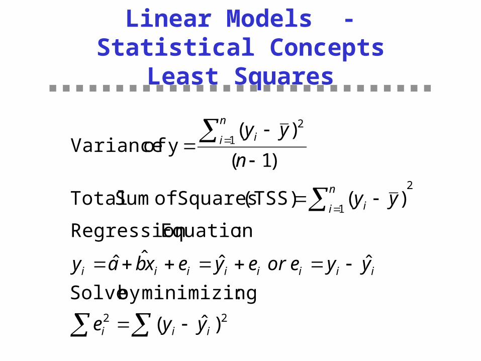
Linear Models - Statistical ConceptsLeast Squares

22

2

1

1

2

)ˆ(

:minimizingbySolve

ˆˆˆˆ

:EquationRegression

)((TSS)SquaresofSumTotal

)1(

)(yofVariance

iii

iiiiiiii

n

i i

n

i i

yye

yyeoreyexbay

yy

n

yy

Linear Models - Statistical ConceptsR2

2

2

2

22

222

)(1

)(

)ˆ(

)ˆ()(

yy

e

TSS

RSSTSS

TSS

ESS

yy

yyR

ESSRSSTSS

yyeyy

i

i

i

i

iii

Nonlinear Response Models: ADBUDG

b – minimum Y

a – maximum Y

c – shape, 0 < c < 1 concave; c > 1 s-shaped

d – works with c to determine specific shape

0)(

XdX

XbabY

c

c

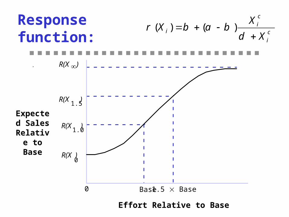
Response function:

Expected Sales

Relative to

Base

Base

R(X )

R(X ) 1.5

R(X ) 1.0

R(X ) 0

0 1.5 Base

Effort Relative to Base

ci

ci

iXd

XbabXr

)()(

ADBUDG Model

• Examples:– Response Modeler: units of marketing effort and sales

– Conglomerate: four cities responding to sales promotion

– Spreadsheet Exercise: (Blue Mountain Coffee) sales response to advertising

– Syntex: 7 products or 9 specialties responding to number of sales calls

– John French: 4 accounts responding to call frequency

Using Solver to Estimate Response Functions

• Locate parameters and choose starting values

• Create columns for independent and dependent variables. Calculate mean of dependent variable.

• Create column of predicted dependent variables based on parameters and independent variables.

• Create column of squared errors between actual and predicted dependent variable. Sum this column.

• Use solver to search over parameters to minimize sum squared errors.

Judgmental Calibration of ADBUDG

• Data: R(Xminimum), R(Xsaturation), R(X1.0), and R(X1.5)

• Parameters:

• a = R(Xsaturation)

• b = R(Xminimum)

• d = (a-R(X1.0))/(R(X1.0)-b)

• c = ln((d*(R(X1.5)-b)/(a-R(X1.5))/ln(1.5)

Judgmental Calibration of ADBUDG

• Data: R(Xminimum), R(Xsaturation), R(X0.5), R(X1.0), and R(X1.5)

• Parameters: • a = R(Xsaturation), b = R(Xminimum)• d = (a-R(X1.0))/(R(X1.0)-b)• Solve for c using least squares over R(X0.5) and R(X1.5)

))(()()(ˆ)(

))(()()(ˆ)(

ˆ5.1

ˆ5.1

5.15.15.15.1

ˆ5.

ˆ5.

5.5.5.5.

dX

XbabXRXRXRe

dX

XbabXRXRXRe

c

c

c

c

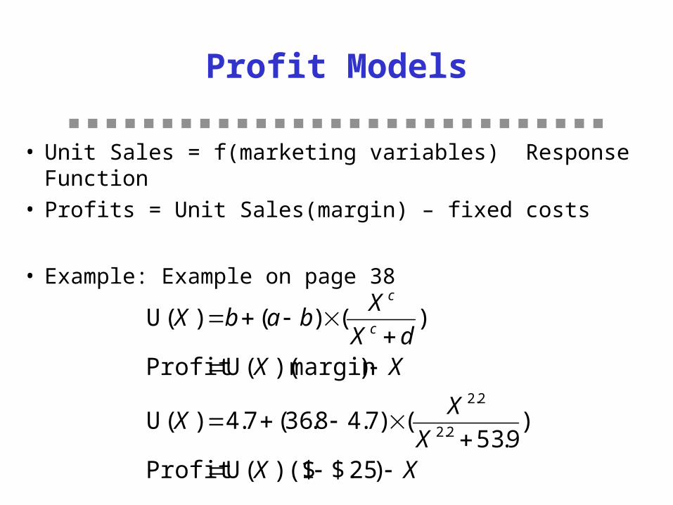
Profit Models

• Unit Sales = f(marketing variables) Response Function• Profits = Unit Sales(margin) – fixed costs

• Example: Example on page 38

XXX

XX

XXdX

XbabX

c

c

)25$.1)($(UProfit

)9.53

()7.48.36(7.4)(U

)margin)((UProfit

)()()(U

2.2

2.2

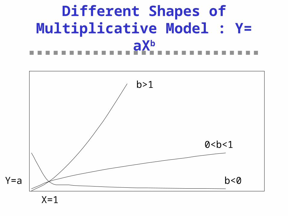
Different Shapes of Multiplicative Model : Y= aXb

0<b<1

b<0

b>1

X=1

Y=a

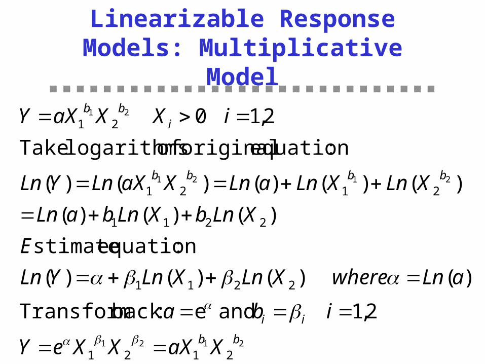
Linearizable Response Models: Multiplicative Model

2121

2121

21

2121

2211

2211

2121

21

2,1 and e :backTransform

)()()()(

:equationstimate

)()()(

)()()()()(

:equationoriginal of logarithms Take

2,10

bb

ii

bbbb

ibb

XaXXXeY

iba

aLnwhereXLnXLnYLn

E

XLnbXLnbaLn

XLnXLnaLnXaXLnYLn

iXXaXY

Multiplicative Models Cont’d

• Estimate judgmentally– Sales at current level of marketing variable(s)

– Percent change in sales for a percent change in marketing variable i = exponent bi

– Yc=a Xcb

– Solve for a

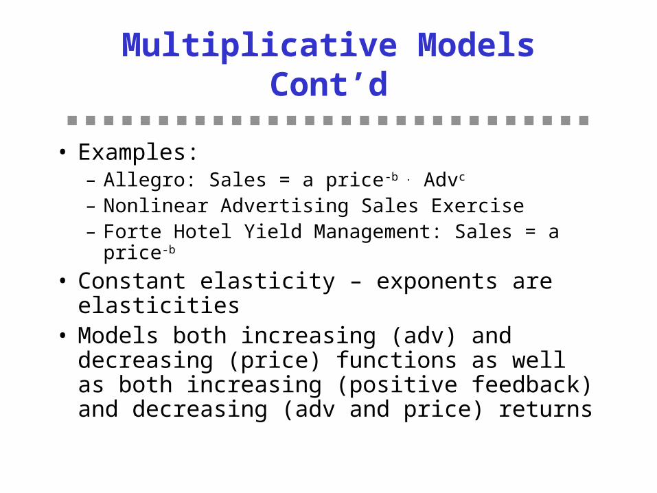
Multiplicative Models Cont’d

• Examples:– Allegro: Sales = a price-b . Advc

– Nonlinear Advertising Sales Exercise– Forte Hotel Yield Management: Sales = a price-b

• Constant elasticity – exponents are elasticities• Models both increasing (adv) and decreasing

(price) functions as well as both increasing (positive feedback) and decreasing (adv and price) returns

Other Linearizable Models

• Exponential Model: Y = aebx; x > 0– Ln Y = Ln a + bX– Models increasing (b>1) or decreasing (b<1) returns .

• Semi-Log Model: Y = a + b Ln X • Reciprocal Model: Y = a + b/X = a + b (1/X)

– Models saturation

• Quadratic Model: Y = a + bX + c X2

– Supersaturation– Ideal points in MDS– Bass Model

Choose model based on:

• Theory• Fit• Pattern of error terms• Signs and T-statistics of coefficients

Response Function

CurrentSales

Response Function

Min

Max

Current Effort

Sales Response

Effort Level

Elasticity - Percent change in the dependent variable divided by the percent change in the independent variable

= (Y/Y)/(X/X) = (Y/X) (X/Y) = (dy/dx)(X/Y)

• If Y = bX then = 1 For example, if we double X (from x to 2x), Y also doubles (from bx to 2bx), so the percent change in X is always the same as the percent change in Y.

• If Y = a + bX, then Y/X = b(x)/ x = b and X/Y = X / (a + bX) and = (Y/X) (X/Y) = bX/(a+bX) <1 if a>0

Elasticities with a Multiplicative Model

Y = aXb

= (dy/dx)(X/Y)

• dy/dx = a bXb-1

= (a bXb-1) (X/aXb) = (a bXb-1 X)/aXb = b

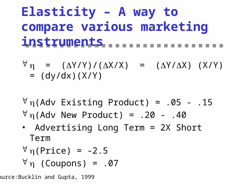
Elasticity – A way to compare various marketing instruments

= (Y/Y)/(X/X) = (Y/X) (X/Y) = (dy/dx)(X/Y)

(Adv Existing Product) = .05 - .15 (Adv New Product) = .20 - .40• Advertising Long Term = 2X Short Term (Price) = -2.5 (Coupons) = .07

Source:Bucklin and Gupta, 1999

Elasticity in Product Classes where P&G Competes

(Adv) = .039 (Price) = -.541 (Deals) = .092 (Coupons) = .125

Source: Ailawadi, Lehmann, and Neslin 2001

Effect of Increasing Advertising

• Assume 100 units sold at $1.00/unit, 50% contribution margin, advertising elasticity of .22, and 10% A/S ratio

• No change in advertising:– Profit = (100 * $.50) - $10 = $40

• A 50% increase in advertising – sales increase by 11%– New Profit = (111 * $.50) - $15 = $40.50

Conglomerate Market Share Calculations – New York

Promotion Level

E4

Response Multiplier

P56

Non-Deal Prone Share

Deal Prone Share

Total Share

E10

0 .4 69% x .05 = 3.45

31% x .05x .4 = .62

4.07

100% 1 3.45 31% x.05 x 1 = 1.55

5.0

150% 1.64 3.45 31% x .05 x 1.7 = 2.635

6.0

Saturation 2.7 3.45 31% x .05 x 2.7 =4.185

7.635

Aggregate Response Models:Dynamics

• Dynamic response model

• Yt = a0 + a1 Xt + Yt–1

Easy to estimate.

Difficult to interpret correctly

currenteffect

carry-overeffect