Markov models of aging: Theory and practice

David Steinsaltz1,∗, Gurjinder Mohan1, Martin Kolb2

Abstract

We review and structure some of the mathematical and statistical models thathave been developed over the past half century to grapple with theoretical andexperimental questions about the stochastic development of aging over the lifecourse. We suggest that the mathematical models are in large part addressingthe problem of partitioning the randomness in aging: How does aging varybetween individuals, and within an individual over the lifecourse? How much ofthe variation is inherently related to some qualities of the individual, and howmuch is entirely random? How much of the randomness is cumulative, and howmuch is merely short-term flutter?

We propose that recent lines of statistical inquiry in survival analysis couldusefully grapple with these questions, all the more so if they were more ex-plicitly linked to the relevant mathematical and biological models of aging. Tothis end, we describe points of contact among the various lines of mathematicaland statistical research. We suggest some directions for future work, includingthe exploration of information-theoretic measures for evaluating components ofstochastic models as the basis for analyzing experiments and anchoring theoret-ical discussions of aging.

1. Introduction: Stochasticity and aging

A famous definition Arking (2006) identifies aging with CUPID develop-ments in an organism — changes that are cumulative, universal, progressive,inherent, and deleterious. And yet, one of the key markers of aging, advanc-ing mortality, is essentially random: for most species we may speak only of auniversally increasing risk of death — force of mortality to the demographers,mortality rate to the biologists, hazard rate to the statisticians. This createspeculiar challenges for mathematical and statistical modeling, since this risk isnot observable or measurable in any single individual. It is an artifact of theensemble.

∗Corresponding authorEmail addresses: steinsal@stats.ox.ac.uk (David Steinsaltz), mohan@stats.ox.ac.uk

(Gurjinder Mohan), kolb@math.lmu.de (Martin Kolb)1Dept. of Statistics, University of Oxford, Oxford OX1 3TG, United Kingdom2Dept. of Statistics, University of Warwick, Coventry, United Kingdom

Preprint submitted to Elsevier June 11, 2012

An important topic of investigation in recent decades has been the scope ofrandomness in aging. There are three fundamentally distinct entry points inthe life course for stochasticity: The beginning, the middle, and the end. At thebeginning of life it appears as inherent variability in the quality of organisms.(This is the main topic of Finch and Kirkwood’s provocative Finch and Kirk-wood (2002).) At the end of life it is the annihilating coup de grace, whether anillness or a predator, that may certainly be facilitated by progressive weakness,but which might have come earlier or later, and not infrequently carry off anorganism in its prime. And in between there are the “thousand natural shocksthat flesh is heir to.”

Suppose we maintain the operationally useful identification of aging withincreasing risk of death. The stochasticity at the end, of the timing of mortality,is not in doubt. Stochasticity at the beginning and during the life course aredifficult to identify. For a given species we face the questions: To what extentwould it be possible, in principle, to sharpen our estimate of an individual’sultimate fate, based on measurements and observations of characteristics presentin the newborn? To what extent are the shocks of life both cumulative and rare,in the sense that they come in large increments that are few enough to yieldidentifiably random trajectories?

In this paper we

1. Describe and structure some of the disparate approaches which have beenpresented, in mathematics and statistics, for examining the stochasticityof the life course, particularly as regards aging and mortality; and

2. Propose how future research could meld these approaches to give clearanswers to the substantive questions of how to account for stochasticityin aging.

1.1. The task of mathematical models

An important distinction between the literature we summarize and the di-rections we outline in section 1.2 and section 4 for current and future researchin aging is in the role assigned to the longitudinal stochastic model. Most ofthe progress in this area in recent years has come from the domain of survivalanalysis, where the goal is fundamentally to measure the effect of covariate mea-sures on hazard rates. When a stochastic model is included, it is commonly akind of large nuisance parameter, whose properties are only abstractly defined,primarily to buttress the parameters estimation against the bias that ariseswhen covariate measurements vary over time. A different perspective, and newtools, are needed to apply survival analysis to examine the nature of unobservedsenescence processes.

Mathematical models have played an important part in our understandingof biological aging for at least the past 50 years: at least since Strehler andMildvan (1960). This celebrated but flawed work is an early version of whatmight be called a mechanistic deterministic model. Mechanistic because themain object of investigation is the internal mechanism of aging, as opposed tothe process by which such mechanisms arise or are maintained. Deterministic

2

because the mechanism explicitly portrays senescence as a loss of function thatprogresses at the same rate in all individuals, as measured by calendar age.

In this paper we will be focused on mechanistic stochastic models of aging:Models which place the variability of aging (and not merely of the consequencesof aging, mortality in particular) at their core.

Why do we need such models? Mathematical models serve, first of all, tosharpen our formulation of theoretical descriptions of the aging process. Theircharacteristics may either be compared to qualitative observations, or insertedas a module into an evolutionary or other teleological model. For such applica-tions the premium is on analytical tractability rather than precise matching toobservable or measurable features of the organism.

Second, mathematical models are an important component of statisticalmodeling. When analyzing aging experiments we rely, whether explicitly orimplicitly, on underlying mathematical models that fit the measurements andother data into a comprehensible and testable framework. For this purposemathematical elegance is less important than an appropriate choice of variables,sufficiently linked to measurable quantities and consequential for the hypothe-ses under consideration. Mathematical tractability or even comprehensibilityrecedes in significance in modern computational methods in statistics, but itremains crucial when we aim to interpret the results, to compare and link themto results of other experiments, and to integrate them with broader theoreticalunderstanding.

1.2. Classifying modelsIn Figure 1 we propose a structure for some of the features typically rep-

resented in statistical models of aging. The ovals represent observable factors,while the rectangles denote characteristics of a hidden layer: Factors which arenot directly observable, but which have most of the causal power in the model.These may be of theoretical interest, or may simplify the description of the ob-served factors. All real models limit themselves to representing explicitly onlysome subset of these factors.

Arrows in the graph represent causal connections. Green ovals representmeasurable features of the organism, while blue rectangles are properties thatare posited either because they are theoretically posited to exist and be signif-icant, or because they are practically useful components of a statistical model.While we have assigned suggestive names to these factors, the distinctions aremeant to be structural. The observable features are:

1. Mortality: The time (and perhaps cause) of death. Observable exceptwhen censored.

2. Age: Time since birth (or whatever counts as birth in the given organism).Not causally affected by anything else.

3. Signs of aging: The visible effect of age. By definition, while this issubject to individual variation, these variations are not directly linked tothe health effects of aging, nor do they affect the progress of senescence.They may be influenced by senescence. The classic examples are gray hairand wrinkles in humans.

3

4. Physiological measures: A catch-all for all visible effects of aging whichdo give evidence of health status. However, as measures they are onlyindicators of the progress of senescence and health, but are not directcauses of mortality or deterioration. Examples are grip strength and verbalfluency. Behavioral changes, such as slower walking or change in clothingpreference, may be included in this category, but to the extent that thesechanges do not influence the future course of senescence.

The unobserved features may be modeled in many different ways; here wecategorize them by the distinction between features that fixed, fluctuating, andcumulatively random. Their fundamental role is represented by their causalconnections to observable features. Of course, in some cases the correlationbetween an unobserved causal feature and an observed measurement or behaviorwill be so tight that the distinction is merely formal.

1. Fixed frailty: These are genetic, epigenetic, and perhaps other inherentcharacteristics of an individual that affect their mortality risk throughouttheir lives.

2. Individual characteristics: These include fixed characteristics of anindividual that influence the expression of senescence, but do not nec-essarily determine mortality: Individual optimum blood pressure, familypredisposition to gray hair, exposure to testosterone in utero, and so on.

3. Health and Senescence: The distinction here is somewhat arbitrary.Health is defined as that which, if it does not kill us, leaves us no weakerthan before. Acute pneumonia, for instance, or an automobile accident.Of course, many illnesses have both an acute phase and chronic damage.It is simply a matter of definition that we designate those cumulativehealth consequences as “Senescence”. It is for this formal reason that acausal arrow points from senescence to health — aging makes itself felt inincreased risks for all manner of nonfatal illnesses — and from health tomortality, but not from health back to senescence.

We note that this graph is restricted to the individual level. A more completemodel of senescence would include social and environmental influences, whichin some species are likely to be of paramount significance.

The general approach we describe here is generically described as “jointmodeling”: In each model there is a mathematical description of some subsetof the unobserved (blue square) aging, and some portion of the observed (greenoval) aging, and a link between them. A complete version would be impossiblycomplex, so every model that has been substantively analyzed simplifies thecausal graph somewhat.

The theoretical demography and biology of aging literature has described asubstantial number of mathematical models that represent formalized versionsof different biological conceptions of the aging process. Each of these couldserve as the infrastructure for a joint model, when linked to a process for gen-erating measurable quantities. The task is to link these in such a way that thehidden model effectively represents and organizes information about observable

4

Senescence

Health(short-term)Fixed Frailty

Individual Characteristics

Age

Mortality

Physiological measures

Signs of aging

Figure 1: Causal graph for a statistical model of aging. Green ovals represent measurablefeatures of the organism, while blue rectangles represent unobserved components of the agingprocess which are presumed by the model. solid arrows show causal effects that are essentialto the nature of the phenomena being described; if these features are present in a model thenit is almost unavoidable that there should be a direct causal link between them. Dashedarrows are more optional causal links.

phenomena, particularly trends in mortality. As we will discuss in section 4.1,according to one way of measuring the statistical utility of a joint model, thepotential value of the senescence factor in some classic models is surprisinglysmall.

2. Markov models: Mathematical theory

Underlying the joint modeling of observed and unobserved aging must be amathematical model of the aging process. While some of the most celebratedaging models, such as Strehler and Mildvan (1960), represent aging itself asdeterministic (Strehler and Mildvan limited stochasticity to the “challenges”that convert the deterministic decline in “vitality” into increased probabilityof death), we focus here on stochastic models, which largely means Markovprocess models. In such a model there is an internal state — often termed a“senescence” or “vitality” state — that evolves randomly, but with no internalstructure or memory of the past trajectory.

We describe here briefly some of the prominent types of mathematical mod-els. A good review article that goes into more depth on a variety of models isYashin et al. (2000).

5

2.1. Crude vitality models

There is a significant body of work proposing simple structures for vitality orsenescence, without any detailed underlying story. Fixed frailty and individualcharacteristics typically play no role in these models, no do the sporadic randomeffects that we have denoted as “health”. An influential example of this styleis the famous “cascading failures” model of Le Bras (1976): Here senescence isa positive integer state (1, 2, 3, . . . ), and an individual in state k moves up tostate k + 1 at a rate proportional to k, and also has mortality rate increasingproportionately to k. We discuss this example at greater length in section 4.1.

Typically attempts to link these kinds of models to data have focused onmortality rates. Le Bras’s original paper purported to show that Gompertz-like mortality would arise, but Gavrilov and Gavrilova (1991) later pointed outthat this model ultimately yields mortality plateaus rather than exponentiallyincreasing mortality. Mortality plateaus were also the object of comparison inWeitz and Fraser (2001), and were comprehensively analyzed in Steinsaltz andEvans (2004). Aalen and Gjessing (2001, 2003) have provided perhaps the mostgeneral applications of this type of model to generating mortality distributions,primarily for biomedical applications. The consequences of vitality as a purelyunobserved process driving mortality have been perhaps most thoroughly de-veloped by T. Li and J. Anderson Li and Anderson (2009).

Yashin et al. (1994) first made explicit the inescapable weakness of attemptsto infer from mortality data back to the process of aging: Models with funda-mentally different longitudinal structures produce the same mortality rates. Ifwe observe only the binary variable dead or alive, it is a challenge even to inferthe mortality rates. Interpreting the underlying process driving the mortalityrates is impossible. Yashin and Manton (1997) brought the study of joint mod-els of covariates with mortality into the ambit of aging studies. More recentdevelopments, particularly of Yashin and his collaborators, will be discussed insection 3.1. In recent years the linking of vitality models to individual longitu-dinal data has become a major focus of statistical work in clinical trials and ingerontology.

2.2. Reliability-type models

The link between the wearing out of mechanical devices and the senescentdecline of organisms has been treated as the intuitively obvious foil to more so-phisticated theories at least since Weismann (1892) in the 19th century. In the1970s and 1980s a number of theorists proposed specific mathematical modelsintended to formalize this intuition. Early pioneers of reliability models in East-ern Europe were Gavrilov and Gavrilova (1991, 2001), Koltover (1982, 1997),and Doubal (1982); their counterparts in the west include Rosen (1978) and Wit-ten (1985). All presented elementary stochastic models that aimed to produceage-specific increasing mortality from non-aging components. To the extentthat these models have been linked to data, this was done in a rudimentaryway, typically by comparing broad features of predicted and observed mortalitycurves. More recently some researchers, in particular Pletcher and Neuhauser

6

(2000) and Laird and Sherratt (2009) have embedded reliability models of agingwithin the framework of mathematical models of evolution.

More recently, statistically sophisticated versions of engineering reliabilitymodels have started to be applied to problems close to the concerns of agingresearch, under the name “degradation models”. These are described in section3.3.2.

2.3. Damage-accumulation models

One of the most influential modern theories of aging, “disposable soma”Kirkwood (1977), takes a slightly different approach to the accumulation ofdamage by blending the long tradition of metabolic theories of aging (goingback to Pearl (1928)) with Orgel’s error catastrophe Orgel (1963). It is anoptimization theory, of the sort that suggests that the apparent inefficiency ofsenescence is an illusion of not appropriately weighing the alternatives, or notconsidering the tradeoffs that would be required to incorporate perfect repair.

This theory has directly or indirectly inspired a long line of what might becalled “metabolic budget” models. Instead of trying to model the componentsand structures whose performance degrades over time — something that Kirk-wood himself essayed in two impressive papers Kowald and Kirkwood (1994,1996) — damage as such is quantified as it accumulates in cells and organ-isms, is repaired or not, and is removed or diluted through reproduction. Inbroadest terms these models link together an organism’s growth, reproduction,damage accumulation and damage repair by some kind of budgeting constraint,and then maximizes fitness by dynamical programming or some other method.This is a large literature, but a few of the signal contributions are Abrams andLudwig (1995); Cichon (1997); Mangel (2001); Chu and Lee (2006); Drenos andKirkwood (2005). The strength of this work lies in the ability to illustrate thedifferent paths that a fitness-maximizer could take in subverting survival to se-lectively relevant goals. The weakness is that the tradeoffs which are at thecore of the theory are represented purely abstractly, by functional relations thathave little justification other than mathematical or computational convenience.

One novel line of research restores the inherent stochasticity of damage ac-cumulation. The mathematical work here, particularly Johnson and Mangel(2006); Evans and Steinsaltz (2007); Watve et al. (2006), has been inspired, atleast in part, by a new generation of aging experiments — Webb and Blaser(2002); Stewart and Taddei (2005); Lindner et al. (2008) — in protozoans, aswell as by the theoretical and science-historical ideas of Bell (1988). In somesense these models reverse the burden of proof — rather than “explaining”senescence they seek to explain reproduction as a tool for disposing of damagethat has accumulated over a lifetime. The link between reproduction and senes-cence is productively problematized when modeling the senescence of organismsthat have no clear individual beginning, hence only at best a partial cleansingof accumulated damage through reproduction.

We will not describe in detail the statistical side of these models, but a mod-est body of statistical theory and methodology has been built up in very recenttime — cf. Bansaye et al. (2011); Delmas and Marsalle (2010); de Saporta et al.

7

(2011) — inspired by the requirements of the experiments. These permit statis-tical tests of the hypothesis that organisms are dividing their damage unequally,as well as hypotheses that damage allocation is linked to future measured vital-ity.

2.4. Fixed-frailty models

There is a class of models that simply attempts to capture the variabilityin individual trajectories through a fixed variability in a basic individual char-acteristic, such as individual hazard rate. This idea was notably applied tothe analysis of mortality plateaus in Vaupel et al. (1979) and Vaupel and Carey(1993). In Yashin et al. (1994) it was pointed out how it is essentially impossibleto distinguish fixed-frailty from Markov models simply by observing mortalityrates. This observation is an important motivation for joint modeling in agingstudies.

Many of the models and techniques used in this work come originally fromreliability theory in engineering. A review of mathematical and statistical the-ory of mixture models, including some applications to survival models, may befound in McLachlan and Peel (2000). The asymptotic behavior of fixed-frailtymodels, particularly as regards their long-term hazard rates, has been describedin Finkelstein and Esaulova (2006) and Steinsaltz and Wachter (2006).

3. Markov models: Statistical applications

Consider a survival experiment. The data from such an experiment mayinclude survival times (possibly censored), some measurements of permanentcharacteristics for each individual (including birthdate), and some longitudinalmeasurements of time-varying characteristics of each individual.

Such data provide a natural testbed for stochastic theories of aging. Differenttheories make different predictions about the relative strength of fixed and time-varying deterministic factors, and fixed and time-varying stochastic factors, indetermining the future life course. Much of the published literature is centeredon the remaining lifetime as the principle observable, reflecting in part theconstraints of earlier experiments and studies. We will retain this perspectivein much of the discussion to follow, but the reader should keep in mind thatthere is no reason, in principle, why survival needs to be at the center of agingstudies, once longitudinal data are being collected.

3.1. Joint longitudinal survival

With the increasing number of long-term studies in recent decades has comea flowering of research on the statistical problem that arise when combininglongitudinal measures with survival data. We give only a brief summary here,directed at the particular concerns of this paper. For further statistical back-ground we recommend consulting some of the many excellent reviews of thejoint longitudinal survival modeling literature to date, including Troxel (2002);

8

Tsiatis and Davidian (2004); Yu et al. (2004); Ibrahim et al. (2005); Verbekeet al. (2010); Sousa (2011).

Methods for analyzing survival data jointly with longitudinal observationsmay be sorted into three categories:

1. The simplest approach separates the longitudinal and survival analysesinto a 2-stage analysis where in the 1st stage, a longitudinal model, suchas a linear mixed effects model, is estimated for the covariates ignoringsurvival information; at the 2nd stage the fitted values from this model,are plugged into a standard survival model, such as Cox proportionalhazards model, as time-dependent covariates Tsiatis et al. (1995); Bycottand Taylor (1998); Dafni and Tsiatis (1998).

2. A more demanding approach bases estimation and inference on a jointlikelihood for the longitudinal covariates and survival analysis, within theframework of classical statistical models. Typical joint likelihood construc-tions are based on a linear mixed effects model for the subject-specific co-variate trajectories and a Cox proportional hazards model. In the languageof section 1.2, these tend to be based on age, individual characteristics,fixed frailty, and health. That is, time-varying components are determin-istic, while random effects are either fixed for all time (sometimes in theform of an individual rate of change) or short-term.

3. A number of recent studies have attempted to model more directly the cu-mulative random component of senescence, allowing an unobserved senes-cence process to drive mortality, but also some physiological measures andsigns of aging. As we have discussed, there is a wealth of existing stochas-tic senescence models — generally Markov models — that could be usedas the hidden component of such a joint model, but efforts to exploit thisstockpile, and explore the statistical utility of these theoretical modelshave so far been sporadic.

The first approach ignores survival information when modeling the longitu-dinal process, and consequently underestimates the uncertainty in the estimatedvalues of survival parameters. Numerous authors highlight the resulting ineffi-ciency, and endorse the second approach, including Faucett and Thomas (1996);Wulfsohn and Tsiatis (1997); Yu et al. (2004); Sweeting and Thompson (2011).

The second and third approaches are versions of joint modeling. We de-scribe here some of the essential features of current joint modeling methods.A joint likelihood approach is expected to provide more precise estimates ofthe relationship between the longitudinal process and time to event, as well asbeing more efficient in its use of the data, cf. Wulfsohn and Tsiatis (1997); Yuet al. (2004). The third approach is distinguished by its reliance on a stochas-tic process model, which could allow it to better capture (and measure) thestochasticity in the longitudinal component. The main drawback is that thisexpands the scope for arbitrary choice to the component of the model that isinherently least subject to verification by direct observation, thus complicatingresponsible efforts at model selection and verification.

9

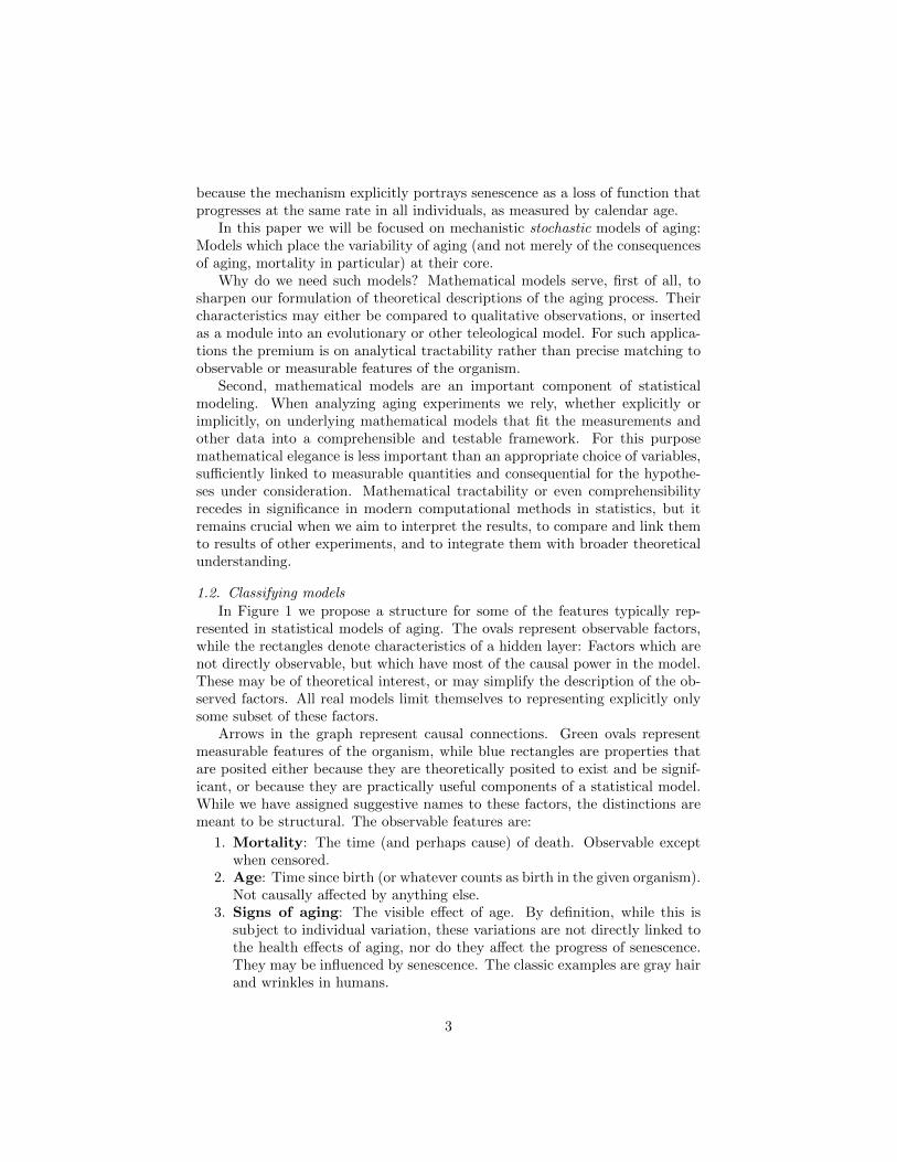
Let Zi(t) denote the latent true covariate value for a process at time t forthe ith subject and Xi(t) denote the corresponding longitudinal measurementavailable for the process; let Zi(t) = {Zi(u), u ≤ t} denote the ‘true’ historyof the process up till time t and Xi(t) the corresponding observed longitudinalmeasurements up till time t; let Ti denote the observed survival time for the ithsubject and Yi any other time-independent covariates for the ith subject.

Tsiatis et al. (1995) propose a joint model based on a linear mixed effectsmodel:

Xi(t) = Zi(t) + ε(t), (1)

Zi(t) = θ0i + θ1it, (2)

where ε(t) denotes the measurement error with E(ε(t)) = 0, Var(ε(t)) = σ2 andCov(ε(t1), ε(t2)) = 0 for t1 6= t2. The random effects θi = (θ0i, θ1i) given Yi arebivariate normal with fixed parameters.

The random intercepts and slopes for each subject can then be combinedwith the hazard of failure within a larger ‘metamodel’, using the Cox propor-tional hazards framework, as in Wulfsohn and Tsiatis (1997) and Yu et al.(2004):

hazard rate = λ(t | θi, Zi(t), Yi) = λ0(t)exp[γ(θ0i + θ1it) + βZi], (3)

where γ and β are regression coefficients for the time-dependent and time-independent covariates.

Several authors, particularly Wang and Taylor (2001), but also Taylor et al.(1994) and LaValley and DeGruttola (1996), expand (2) by including an in-tegrated Ornstein-Uhlenbeck (IOU) stochastic process. This is a continuousversion of an autoregressive process, so the effect is to expand the range ofstochasticity to include a process of medium-term memory:

Xi(tij) = Zi(tij) + εij , εij ≈ N(0, σ2e), (4)

Zi(t) = ai + bt+ βXi(t) +Wi(t), (5)

where tij refer to the time points j at which values were measured for subject i;ai ≈ N(µa, σ

2a) and Wi(t) denotes the IOU process. Henderson et al. (2000) and

Xu and Zeger (2001) consider Wi(t) to be a stationary gaussian process, whichenables the trend to vary with time and allows a within-subject autocorrelationstructure which can be thought of as biological fluctuations about a smoothtrend, as formalized by Tsiatis and Davidian (2004).

The accelerated failure-time (AFT) model — cf. Cox and Oakes (1984) —offers a viable alternative to the Cox proportional hazards model when the pro-portionality assumption breaks down. Wei (1992) and Cox (1997) in particularhighlight how modelling covariates directly on the survival time can provide amore intuitive understanding of the relationship between a longitudinal processand the survival time. An AFT model formalizes the notion of each individualhaving his or her own senescence clock, with mortality, physiologic changes, and

10

signs of aging all being driven by this hidden internal clock, hence only indi-rectly by calendar time. In Hsieh et al. (2005) a joint longitudinal-AFT model isproposed, which models the longitudinal process by a linear mixed effects mea-surement error model, as in the examples described above. Swindell (2009) hasalso recommended the AFT as a useful statistical framework for aging research.The statistical techniques for accelerated failure are not yet as well developedor as easy to use as for proportional hazards.

3.2. Physiological measures with error

In many of the earliest versions of joint modeling of survival with longitudinalcovariates the cumulative factor that drives mortality rates — is not an abstract“senescence” quality, but a concrete physiological feature. It is not observablebecause of the limitations of measurement. An important early example is CD4count in HIV studies Wulfsohn and Tsiatis (1997), where the crucial factor issubject to measurement error and short-term fluctuations (“short-term health”in the language of section 1.2).

Longitudinal data such as the physiological measurements can be fitted in aCox proportional hazards model as time-dependent covariates Cox and Oakes(1984) but as Sweeting and Thompson (2011) note, this is not recommended.Typically, the longitudinal measurements are incomplete and prone to measure-ment error and simply using the raw measurements as recorded, can lead tobiased estimation of model parameters, as discussed by Prentice (1982); Hughes(1993); Raboud et al. (1993); Hu et al. (1998).

Lange et al. (1992) and Hoover et al. (1992) draw further attention to thehigh variability within subjects when making biological and physiological mea-surements. In response, longitudinal models are typically used when fittingcovariates measured over time, with error. Carroll (2006) provides a compre-hensive review of the models currently available.

3.3. Applications to aging

In recent times, joint longitudinal survival models have been extended toinclude and build upon on the earlier aging models, some of which we haveoutlined in section 2. In principle, almost any mathematical model may serveas the engine of a joint model. It is important to be aware of the theoreticalimplications and constraints imposed by the choice of longitudinal model, andto consider these as seriously as questions of statistical tractability.

3.3.1. Modeling signs of aging

A number of existing statistical methodologies have been applied recently tothe problem of inferring underlying senescence from longitudinal observationsof signs of aging — that is, in the terminology of section 1.2, measurements ofproperties that do not themselves participate in the causal processes of senes-cence, but are presumed to be influenced by senescence.

Pavlov (2010) builds upon the joint modeling ideas of Wang and Taylor(2001),Taylor et al. (1994), and LaValley and DeGruttola (1996) by applying a

11

Kalman filtering approach of the sort that was introduced by Fahrmeir (1994)for discrete-time survival data. Using the hidden Markov model setting of astate space model he explores the dynamics of an unobserved aging processbased on damage accumulation and other stochastic aging theories. An at-tempt to capture heterogeneity is made through the introduction of a frailtycomponent within the joint longitudinal survival likelihood. Using fruit-fly life-time behavioral data (from the studies described in Zou et al. (2011)), Pavlov(2010) postulates the hidden aging process to follow Brownian motion, an IOU,or other basic stochastic processes. This allows him to extract an aging signal ofsorts from observed fly eating habits over age. Pavlov’s approach highlights theflexibility of a state-space model — based on an unobserved process driving thesystem — to explore and model the aging process. The unobserved process canbe considered as the latent aging process and models can be tailored to extractaging information from a wide variety of data. The direct conclusions of thiswork were limited by the very small number of individual flies included in thestudy.

Yashin et al. (2007), on the other hand, propose stochastic differential equa-tions for capturing physiological changes in a joint longitudinal survival setting.They in particular advocate the use of stochastic differential equations for cap-turing allostasis and the decline in adaptive capacity associated with aging.But as Yashin et al. (2011) later remark, this fails to describe changes in ‘healthstatus accompanying physiological aging’, unlike Pavlov (2010). Yashin et al.(2011) uses the notion of a health history — modeled using a finite state jump-ing stochastic process — and attempts to jointly analyze this with physiologicalmeasurements and survival, as in Yashin et al. (2007).

A different approach was introduced by Muller and Zhang (2005). Usingfunctional principal component analysis (Rice and Silverman, 1991) and theconcept of functional regression (Cardot et al., 2003) from functional data anal-ysis (cf. Ramsay and Silverman (2005)) they construct a time-varying functionalregression framework that predicts the remaining lifetime and lifetime distribu-tions from longitudinal trajectories for individual subjects. They remark, as wehave emphasized here, that in studies on aging the predicted remaining lifetimecan provide a useful measure for senescence.

3.3.2. Degradation models

Aging is often defined as the accumulation of damage or wear and tear overtime leading to death. Degradation models thus provide a useful alternativeframework for analysing survival data by linking failure times with stochastictime-varying covariates. Singpurwalla (1995) provides key early expository workoutlining useful stochastic processes for modeling degradation and stochastic‘wear and tear’, which can be related to the biological ‘damage accumulation’aging theory.

From the perspective of aging research, it is notable that Whitmore et al.(1998) introduced a failure time model based on a bivariate Wiener process,whereby one process represents an observed marker process, and the secondrepresents a latent process. The failure time is defined by the latent process

12

crossing a threshold. Lee et al. (2000) extended this to model a joint markerprocess and latent health status; as with the hidden diffusion “senescence state”analyzed by Pavlov (see above), the notion of a latent health status is appealing,since it represents the ‘unobservable’ aging process.

Degradation models are a distinct scientific lineage from joint survival mod-els, and there is limited cross-citation between them, but they are formallyalmost identical. The two approaches have tended to emphasize different con-cerns, reflecting their divergent origins: Degradation models grew out of reli-ability modeling in engineering, while joint survival modeling are one of themany adaptations of classical survival analysis in medicine to the problems oflongitudinally measured covariates.

Building on the work of Whitmore et al. (1998) and Lee et al. (2000), Lee andWhitmore (2006) introduced ‘threshold regression’ for survival data by postulat-ing the deterioration of a subject’s health as following a stochastic process andthereby utilising first-hitting time model ideas as previously — see Aalen andGjessing (2001) for a comprehensive review of first-hitting time models. Follow-ing the notation in Lee and Whitmore (2006), let {X(t), t ≥ 0} denote a Wienerprocess with mean µ and variance σ2, with initial value X(0) = x0 > 0. Withµ < 0 the process will tend to drift towards 0 and hence the first-hitting timefor the zero level follows an inverse Gaussian distribution. Lee et al. (2010)extended these ideas to introduce a threshold survival regression model withtime-varying covariates in a health status setting, and further advances by Liand Lee (2011) allow for more flexible representation of the varying coefficients.

Some more recent work on degradation models such as Bagdonavicius andNikulin (2000) and Bagdonavicius and Nikulin (2004) incorporate longitudinalmeasures, producing a framework that differs only in nomenclature from thesurvival models. However, instead of the Gaussian-process models that domi-nate the joint-modeling literature, this work reflects its engineering influencesby building upon a gamma process, which has substantially different properties.Most importantly, it only increases, so it represents a model of aging with “wearand tear” but no repair.

3.3.3. Discrete state-spaces and deficit models

Discrete-state models like the Le Bras mortality model offer some importantsimplifications relative to continuous-state models. They are particularly ap-pealing for settings where the observations fall naturally into discrete orderedclasses. For example, Mesbah et al. (2004) use a simple four-state model (good,neutral, bad, dead) to analyze joint observations of longitudinal quality of lifereports and survival. This work is very much in the spirit that we are advo-cating here, since the goal is not merely to use the longitudinal observations topredict mortality, but also to understand the quality-of-life process itself.

A substantial body of work by A. Mitnitski and K. Rockwood, together withvarious collaborators — in particular Mitnitski et al. (2002) and Rockwood andMitnitski (2007) — has promoted the use of simple counts of discretely observ-able physical deficits as a proxy for ageing. This stands currently as one of themost thorough attempts to date to measure the individual pace of biological

13

aging in humans, and to validate the measurement procedures through a rangeof statistical, epidemiological, and mathematical modeling methods. Interest-ingly, their preferred mathematical model (Mitnitski et al. (2006)) representsthe frailty index itself as Markov, with no hidden layer. It is not clear from thepublished record what efforts were made to validate this feature of the model,or if any alternatives were considered.

4. Future work: Integrating the mathematical and statistical per-spectives

We have described developments in theoretically modeling aging systems interms of the progressive changes in measurable senescence states, and in linkingmeasured longitudinal changes statistically to survival. There are still impor-tant gaps in our understanding, which need to be addressed before this work caneffectively shape our view of biological aging. We discuss here two of these gaps,which fall in the space linking mathematical and statistical approaches: Eval-uating the effectiveness of a senescence model, and parcelling out stochasticityautomatically among different timescales.

4.1. Evaluating the potential significance of Markov models

Suppose we are faced with a choice between various models of senescence,one of which instantiates an individual inherent robustness, another which addsa random slope of vitality loss, a third with “health” variation, representedas stochastic short-term fluctuations in vitality. Considered as a statisticalproblem, given a collection of covariate measures (linked to the vitality) andoutcomes we have a variety of tools for deciding which model best connects thecovariates to the outcomes.

In the biostatistical practice of survival analysis it is common to focus onpredictive accuracy: We score a model based on the average difference betweenthe best prediction we can make of the lifetime from the model and the truelifetime. If the average is judged in the mean-square sense, we obtain the Brierscore or conditional mean square error of prediction in Lawless and Yuan (2010).In the simplest setting, where we know the true model (so we are not using theobservations to estimate the model) the Brier score is essentially the expectedresidual variance when the survival is conditioned on the covariates.

For purposes of selecting relevant factors for a theoretical model of agingit is reasonable to foreground not the potential prediction accuracy, but ratherthe opposite: How much does the distribution shift when we incorporate a newmeasurement into the model. For the remainder of this section we will continueto assume that the model is known.

4.1.1. Stable covariates

Suppose for the moment we are considering inherent individual properties,measuring stable covariates which are fixed throughout life, represented by anunderlying characteristic Z or a measurement X. If π is the distribution of

14

T , and πz is the conditional distribution, given that the covariates Z havevalue z, then the value of the information Z = z is just δ(π, πz) — the changein our evaluation of the distribution of T that comes from incorporating theinformation {Z = z} — and the average value of Z is

EZ [δ(π, πZ)] , (6)

where the expectation EZ gives us the mean distance between the unconditionaldistribution and the conditional distribution. For instance, if π and π′ havemeans µπ and µπ′ , and the quadratic distance δ(π, π′) = (µπ − µπ′)2, then thedistance in (6) turns out to be precisely the difference between the variance ofπ and the average residual variance conditioned on Z.

The same arguments apply with comparable force to other measures of effi-cacy of a covariate model. One appealing possibility for the distance is Kullback-Leibler divergence (not, formally speaking, a true distance). In this case, thevalue of Z for predicting T becomes the same simply the mutual informationbetween T and Z:

I(T ;Z) = E[∫ ∞

0

f(t) logf(t)

fZ(t)dt

].

To take a simple example, suppose Z is the sex of an individual, with afraction p of the population being male and 1− p female, and that the survivaltimes for male and female have different distributions with densities fF andfM , with means µM and µF respectively. The overall mean lifespan is thenµ = pµM + (1− p)µF . Using the quadratic distance defined above, the “value”of knowing that an individual is female for predicting lifespan is (pµM − pµF )2,and the value of knowing that an individual is male is ((1−p)µM − (1−p)µF )2.The average value of knowing an individual’s sex weights these two values by theappropriate proportion in the population, yielding p(1−p)(µM−µF )2. This hasa natural interpretation: Sex is informative for lifespan when there is a largedifference between male and female life expectancy, but also when there areequal numbers of male and female. In the extreme case, where the populationis nearly all of one sex, observing an individual’s sex tells us on average verylittle about survival time.

If we do not observe the individual’s sex directly, but only a covariate Xthat is correlated with sex (and otherwise independent of survival time — forexample, the individual’s name or hair length) then the factor p(1−p) is replacedby a smaller factor p(1− p)− E[p(X)(1− p(X))], where p(x) is the proportionof males among those with {X = x}.

If we measure value by mutual information, we see that

I(T ;Z) =

∫ ∞0

f(t) log f(t)dt−p∫ ∞0

f(t) log fM (t)dt−(1−p)∫ ∞0

f(t) log fF (t)dt.

(The first term on the right-hand side is the entropy of the survival time.) Thismay be understood as the reduction in the quantity of information (measuredin bits, if the logarithm is base 2) required to specify the survival time, when

15

the sex is known as well. As before, if X is a covariate that is correlated withsex, but otherwise independent of survival time, we have I(T ;X) ≤ I(T ;Z),and

I(T ;Z)− I(T ;X) = I(X,T ;Z)− I(X;Z).

That is, the extra information that knowing Z provides about T over and abovewhat X provides is the same as the increased certainty about the sex acquiredby knowing T and X, compared with just knowing X.

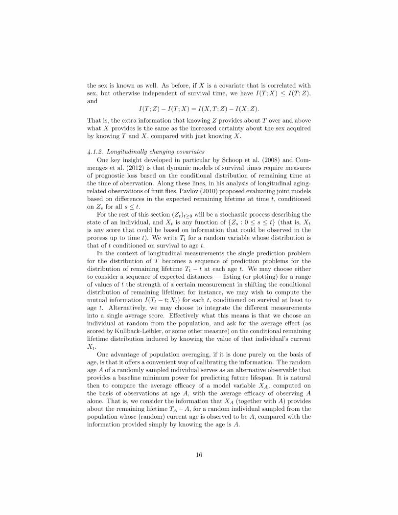
4.1.2. Longitudinally changing covariates

One key insight developed in particular by Schoop et al. (2008) and Com-menges et al. (2012) is that dynamic models of survival times require measuresof prognostic loss based on the conditional distribution of remaining time atthe time of observation. Along these lines, in his analysis of longitudinal aging-related observations of fruit flies, Pavlov (2010) proposed evaluating joint modelsbased on differences in the expected remaining lifetime at time t, conditionedon Zs for all s ≤ t.

For the rest of this section (Zt)t≥0 will be a stochastic process describing thestate of an individual, and Xt is any function of {Zs : 0 ≤ s ≤ t} (that is, Xt

is any score that could be based on information that could be observed in theprocess up to time t). We write Tt for a random variable whose distribution isthat of t conditioned on survival to age t.

In the context of longitudinal measurements the single prediction problemfor the distribution of T becomes a sequence of prediction problems for thedistribution of remaining lifetime Tt − t at each age t. We may choose eitherto consider a sequence of expected distances — listing (or plotting) for a rangeof values of t the strength of a certain measurement in shifting the conditionaldistribution of remaining lifetime; for instance, we may wish to compute themutual information I(Tt − t;Xt) for each t, conditioned on survival at least toage t. Alternatively, we may choose to integrate the different measurementsinto a single average score. Effectively what this means is that we choose anindividual at random from the population, and ask for the average effect (asscored by Kullback-Leibler, or some other measure) on the conditional remaininglifetime distribution induced by knowing the value of that individual’s currentXt.

One advantage of population averaging, if it is done purely on the basis ofage, is that it offers a convenient way of calibrating the information. The randomage A of a randomly sampled individual serves as an alternative observable thatprovides a baseline minimum power for predicting future lifespan. It is naturalthen to compare the average efficacy of a model variable XA, computed onthe basis of observations at age A, with the average efficacy of observing Aalone. That is, we consider the information that XA (together with A) providesabout the remaining lifetime TA−A, for a random individual sampled from thepopulation whose (random) current age is observed to be A, compared with theinformation provided simply by knowing the age is A.

16

We are free to choose any sampling distribution we like for this averaging.One appealing choice is the stationary age distribution of the population underconditions of zero growth. This is the distribution whose density at age t is pro-portional to the probability of survival to age t. This is equivalent to looking ata single birth cohort and taking a uniform random sample of all the moments oflife lived by that cohort, and then predicting each individual’s remaining lifespanat that moment. We illustrate the calculation of mutual information averagedover the stationary age distribution in section 4.1.4 and in the appendix.

Commenges et al. (2012) offer a framework for applying information-theoreticmeasures of prognostic loss in survival models with longitudinal covariates. Inthe context of longitudinal covariates, the mutual information has some usefulproperties. For example, if the process Z· driving senescence is a Markov pro-cess, then by the Data Processing Inequality (Cover and Thomas, 2006, section2.8)

I(Tt − t;Xt) ≤ I(Tt − t;Zt).

That is, the most information about T − t that could possibly be available bytime t would be if it allowed a perfect determination of Zt. To put it somewhatdifferently, to adopt a Markov model is to make a claim that there is a theoreticalupper limit to the predictability of future survival, or indeed of any of thefuture trajectory of an individual. In particular, if the Markov chain is time-homogeneous — that is, if time and/or age have no influence on the processindependent of the internal state — then knowing the age and current state ofan individual provides no further information about the future beyond simplyknowing the current state.

Other measures of the prognostic efficacy of hidden stochastic processes andlongitudinal observations have their own strengths and weaknesses. Several ofthese have been developed and usefully compared in Schoop et al. (2011), boththeoretically and by simulations. These include loss-function approaches likeexpected Brier score and conditional mean absolute deviation, and graphicalapproaches like time-dependent ROC curves and predictiveness curves. Theirframework is more general than ours here, as it includes errors from parametermisestimation and model misspecification.

4.1.3. Graphical tools

A common tool used by epidemiologists in evaluating screening tests is theROC curve, a graphical representation of the tradeoff between true positiveand false positive results — see Fawcett (2006) for background. Suppose we aredesigning a test for predicting whether an individual will have a certain property— for instance, dead within 5 years. We have some candidate measure of riskX, and we want to predict “yes” for anyone whose X score is above a thresholds to be determined. As we move the screening threshold gradually down thenumber of positive results increases, catching an increasing fraction of the truepositive cases, but also of the false positives simultaneously. The ROC curveplots the fraction of true positives captured at threshold s against the fraction offalse positives. It starts at (0, 0) (when s is so high that no one passes the test)

17

and moves up to (1, 1). A completely useless measurement will randomly sampletrue and false positives equally, and so will produce the upward sloping 45◦ line.A perfect predictor will go straight up from (0, 0) to (0, 1) (catching 100% of thetrue positives with no false positives mixed in), and then horizontally to (1, 1).In general we expect to find ROC curves somewhere in between, with superiorpredictors yielding greater separation from the diagonal.

If we think of an observable or non-observable feature of the model as pre-dicting an individual’s death within some fixed T units of time from the present,we have a family of ROC curves, depending on T and on the distribution usedto sample the individuals from the population. Let T become very small wehave what might be called the ROC curve for predicting imminent death, giv-ing a snapshot of risk in the population as stratified by the predictor X. Thisis equivalent to plotting the distribution of hazard rate within the population.In other words, suppose we take a sample from the population — for example,all individuals of a given age, or (as we will do in our example in section 4.1.4)sampled from the stationary age distribution. Let Hx be the total current haz-ard rate of all individuals in the sample with X ≥ x, and let Fx be the fractionof the sample with X ≥ x. The ROC for imminent mortality plots the pairs(Fx,Hx) for all x; when X takes on only discrete values, the points are joinedup linearly.

A slightly different formulation is the Lorenz curve, more commonly used ineconomics, which plots the fraction of true positives against the fraction of thetotal population. Of course, if the true positives are only a small fraction of thewhole population, Lorenz curves and ROC curves are essentially the same. Inthe case of predicting imminent mortality the proportion of true positives in thepopulation goes to 0, so the ROC curve described above is actually identical tothe Lorenz curve.

4.1.4. Example: The Le Bras cascading failures model

Predictive measures have been developed and extensively applied in survivalanalysis, although the dynamic versions that are useful for longitudinal covari-ates are fairly new. What we are advocating here is applying these tools forinterpreting the kinds of stochastic models that underly joint models of survivaland longitudinal measures, and that also play a role in theoretical discussionsof the biology and evolution of aging. When we propose a stochastic model ofaging, in which mortality rates are driven by individual random accumulationof senescence (or random loss of vitality), it seems reasonable that we ought toask how much this model actually differs from the naıve deterministic model, inwhich mortality is determined solely by age. How significant is the variability inremaining lifespan coded in the population’s hidden stratification by senescencestate?

For purposes of illustration we show how these calculations come out for theLe Bras cascading failures model, already mentioned in section 2.1. (For details,see the appendix.) In Figure 2 we show the mutual information of Xs andTs−s for different fixed values of s, for three different choices of the parameters(λ, µ): (0.05, 0.1), (0.1, 0.1), (0.1, 0.05). For example, consider the model with

18

parameters λ = µ = 0.1, and suppose we look at a random individual at age 4,with an eye toward predicting their lifespan. Being told the individual’s value ofX4 reduces our uncertainty about the remaining lifespan by 0.06. On this scalethe full uncertainty of T4 — the entropy — is about 3.1. The entropy changesvery little over age, and is very similar for for the other parameter choices underconsideration here. Thus, knowing X4 removes only a small fraction of the totaluncertainty about remaining lifespan at age 4.

The amount of information obtained by observing the state increases asage advances and the states become more variable. The maximum amountof information is larger when λ is bigger, relative to µ. This makes sense,because larger λ implies a larger dispersion of states for a given age, meaningthat knowing the state is relatively more informative. Nonetheless, the mutualinformation is never more than about 6% of the total entropy.

0 10 20 30 40

0.00

0.05

0.10

0.15

Age

I(X;T)

λ=.1, µ=.05λ=.1, µ=.1λ=.05, µ=.1

Figure 2: Information value of observing the underlying senescence state for predicting re-maining lifespan, as a function of current age.

We note that the information I(Xs;T −s) approaches its maximum value atages s when nearly the entire population has already died. If we consider insteadthe mutual information between state and remaining lifespan for a randomlychosen individual in a random time of life, and compare this to the mutualinformation between age and remaining lifespan, we get the results in Table 1.We see that a very large ratio of λ/µ is needed — meaning a large change insenescence states over an ordinary lifespan — to give the unobserved state asignificant information advantage over simple age. (Calculations may be found

19

in the appendix.)

Table 1: Mutual information of remaining lifespan with age (third column) and current senes-cence state (fourth column) for an individual chosen at random from the stable population inthe Le Bras model of senescence, for several different choices of the parameters.

λ µ I(A;TA −A) I(XA;TA −A)

.01 .1 0.193 0.199

.05 .1 0.194 0.226.1 .1 0.196 0.256.1 .05 0.199 0.309.1 .01 0.224 0.546

The basic lesson is that if a model like this did reflect the underlying truthof senescence, no possible biomarker could yield more information about futurelifespan than observation of the hidden state Xt. Despite the fact that allsurvival is driven by Xt, for significant ranges of parameters observing Xt is (onaverage) of little use in predicting future survival.

As described in section 4.1.3, this principle may be illustrated graphically byplotting ROC curves for the population hazard rate, shown in Figure 3. Herewe plot the fraction of total population hazard that can be accumulated for agiven fraction of the population, using individual age (solid curves) or senescencestate (dashed curves) as the basis of the stratification. We see that for the caseλ = µ = 0.1 current age is not very useful as a predictor of mortality risk; theprediction is improved somewhat, but not enormously, by observing the truesenescence state. Age is a somewhat better predictor when λ is reduced to 0.05,and the information value of senescence state is also significantly increased.

4.2. Stochasticity on different timescales

We suggested in section 1.2 that stochastic models could best be under-stood as partitioning the randomness in aging and mortality across differenttimescales: short-term health events, long-term senescence, inherent robust-ness. As we have already discussed, each mathematical model implies a choiceof one or more unobservable and observable properties, allowing us to explorethe interaction and effects. What is missing is a set of tools that would enableus to assimilate diverse data into a generic model that apportions randomnessacross different timescales and measures their influence on survival.

In principle we could hope to encompass the diverse components in Fig-ure 1 within a hidden diffusion model, taking a proportional hazards or otherlink between the hidden state and the hazard rates. The Wang-Taylor modeldescribed at the end of section 3.1 provides a useful starting point. This decom-poses the vitality status of an individual into a common deterministic trend andindividual intercept, plus a white-noise process (short-term random “health”

20

0.0 0.2 0.4 0.6 0.8 1.0

0.0

0.2

0.4

0.6

0.8

1.0

Population fraction

Haza

rd fr

actio

n

Figure 3: Receiver operator curves for current hazard rate in the Le Bras model for parametervalues (λ, µ) = (0.1, 0.1) (black curves, lower down) or (0.1, 0.05) (red curves,higher up). Thesolid curve represents prediction on the basis of observing the senescence state; the dashedcurve represents prediction based on age. The 45◦ upward-sloping line, corresponds to acompletely informationless predictor.

events, in the nomenclature of section 1.2), plus an integrated stochastic pro-cess (“senescence”). Alternatively, if we choose to model cumulative senescenceas strictly increasing we could use the gamma process favored by Bagdonaviciusand Nikulin (2000), and further developed in their more recent work on degrada-tion models (cf. section 3.3.2). As far as we are aware it is an open question towhat extent the distinction between a hidden process that is strictly increasingand one that rises and falls is an identifiable property, and to the extent that itis, how it might best be inferred from data.

There is no reason, in principle, why the model cannot be extended to in-clude, in addition to the zero-memory and infinite-memory components, stochas-tic processes that revert to the mean on intermediate timescales. Significantprogress has been made in recent years in the estimation of diffusions fromlow-frequency observations — see in particular the early review of estimatingfunction techniques Sørensen (1997) and the introduction of spectral techniquesGobet et al. (2004). More recent work has been undertaken largely with aview to finance and econometric applications, and leave untouched many ofthe natural questions for applications to biological aging (although the workon modeling default risk in finance, such as Nakagawa (2001) and Duffie et al.(2009), is formally very close to the context of aging models).

An important goal would be to analyze separate time-scale components alongthe lines described in section 4.1, to evaluate the leverage that these components

21

of randomness can have over the observable components, above all the survival.

5. Conclusion

There has been a profusion of mathematical and statistical models in recentyears that are intended to describe the senescence process and link it to measur-able features of organisms. What we have described here is only a corner of thisburgeoning literature. We have suggested that more attention will be requiredto linking the biological, mathematical, and statistical approaches to aging, be-fore experiments will be able to provide clear answers to biological questionsabout aging. A more systematic exploitation of theoretical models of aging forapplication to longitudinal individual observations has become imperative.

We have proposed adapting some of the standard information theoretic andgraphical tools used in model selection may be useful for defining the effective-ness and potential applicability of certain mathematical models of aging, and forputting bounds on their potential contribution to the analysis of experimentaldata.

References

Aalen, O. O., Gjessing, H. K., 2001. Understanding the shape of the hazardrate: A process point of view. Statistical Science 16 (1), 1–22.

Aalen, O. O., Gjessing, H. K., 2003. A look behind survival data: Underly-ing processes and quasi-stationarity. In: Lindqvist, B. H., Doksum, K. A.(Eds.), Mathematical and Statistical Methods in Reliability. World ScientificPublishing, Singapore, pp. 221–34.

Abrams, P. A., Ludwig, D., December 1995. Optimality theory, Gompertz’ law,and the disposable soma theory of senescence. Evolution 49 (6), 1055–66.

Arking, R., 2006. The Biology of Aging: Observations and Principles, 3rd Edi-tion. Oxford University Press.

Bagdonavicius, V., Nikulin, M. S., 2000. Estimation in degradation models withexplanatory variables. Lifetime Data Analysis 7, 85–103.

Bagdonavicius, V., Nikulin, M. S., 2004. Semiparametric analysis of degradationand failure time data with covariates. In: Parametric and Semipara- metricModels with Applications to Reliability, Survival Analysis, and Quality ofLife. Birkhauser, Ch. 1, pp. 1–22.

Bansaye, V., Delmas, J.-F., Marsalle, L., Tran, V. C., 2011. Limit theorems formarkov processes indexed by continuous time Galton-Watson trees. Annalsof Applied Probability, 2263–2314.

Bell, G., 1988. Sex and death in protozoa : The history of an obsession. Cam-bridge University Press, Cambridge.

22

Bycott, P., Taylor, J., 1998. A comparison of smoothing techniques for CD4 datameasured with error in a time-dependent Cox proportional hazards model.Statistics in medicine 17 (18), 2061–2077.

Cardot, H., Ferraty, F., Mas, A., Sarda, P., 2003. Testing hypotheses in thefunctional linear model. Scandinavian Journal of Statistics 30 (1), 241–255.

Carroll, R., 2006. Measurement error in nonlinear models: a modern perspective.Vol. 105. London: CRC Press.

Chu, C. Y., Lee, R. D., March 2006. The co-evolution of intergenerational trans-fers and longevity: an optimal life history approach. Theoretical PopulationBiology 69 (2), 193–2001.

Cichon, M., 1997. Evolution of longevity through optimal resource allocation.Proceedings of the Royal Society of London, Series B: Biological Sciences 264,1383–8.

Commenges, D., Liquet, B., Proust-Lima, C., 2012. Choice of prognostic es-timators in joint models by estimating differences of expected conditionalKullback–Leibler risks. Biometrics, no–no.URL http://dx.doi.org/10.1111/j.1541-0420.2012.01753.x

Cover, T. M., Thomas, J. A., 2006. Elements of Information Theory. John Wiley& Sons.

Cox, D. R., 1997. Some remarks on the analysis of survival data. Lecture Notesin Statistics, 1–10.

Cox, D. R., Oakes, D., 1984. Analysis of survival data. London: Chapman &Hall.

Dafni, U., Tsiatis, A., 1998. Evaluating surrogate markers of clinical outcomewhen measured with error. Biometrics, 1445–1462.

de Saporta, B., Gegout-Petit, A., Marsalle, L., December 16 2011. Asymme-try tests for bifurcating auto-regressive processes with missing data, preprintavailable arxiv.org/abs/1112.3745.

Delmas, J.-F., Marsalle, L., 2010. Detection of cellular aging in a Galton-Watsonprocess. Stochastic Processes and their Applications 120 (12), 2495–2519.

Doubal, S., 1982. Theory of reliability, biological systems and aging. Mechanismsof Ageing and Development 18, 339–53.

Drenos, F., Kirkwood, T. B. L., 2005. Modelling the disposable soma theory ofageing. Mechanisms of Ageing and Development 126, 99–103.

Duffie, D., Eckner, A., Horel, G., Saita, L., October 2009. Frailty correlateddefault. Journal of Finance 64 (5), 2089–2123.

23

Evans, S. N., Steinsaltz, D., 2007. Damage segregation at fissioning may increasegrowth rates: A superprocess model. Theoretical Population Biology 71 (4),473–90.

Fahrmeir, L., 1994. Dynamic modelling and penalized likelihood estimation fordiscrete time survival data. Biometrika 81 (2), 317–330.

Faucett, C. L., Thomas, D. C., 1996. Simultaneously modelling censored sur-vival data and repeatedly measured covariates: a Gibbs sampling approach.Statistics in Medicine 15 (15), 1663–1685.

Fawcett, T., 2006. An introduction to ROC analysis. Pattern Recognition Let-ters 27, 861–74.

Finch, C. E., Kirkwood, T. B. L., 2002. Chance, Development, and Aging.Oxford University Press.

Finkelstein, M., Esaulova, V., 2006. Asymptotic behavior of a general class ofmixture failure rates. Advances in Applied Probability 38 (1), 244–62.

Gavrilov, L. A., Gavrilova, N. S., 1991. The Biology of Lifespan: A QuantitativeApproach. Harwood Academic Publishers, Chur, Switzerland.

Gavrilov, L. A., Gavrilova, N. S., 2001. The reliability theory of aging andlongevity. Journal of Theoretical Biology 213, 527–45.

Gobet, E., Hoffmann, M., Reiß, M., 2004. Nonparametric estimation of scalardiffusions based on low frequency data. Annals of Statistics 32 (5), 2223–53.

Henderson, R., Diggle, P., Dobson, A., 2000. Joint modelling of longitudinalmeasurements and event time data. Biostatistics 1 (4), 465.

Hoover, D., Graham, N., Chen, B., Taylor, J., Phair, J., Zhou, S., Munoz, A.,et al., 1992. Effect of CD4+ cell count measurement variability on stagingHIV-1 infection. Journal of acquired immune deficiency syndromes 5 (8), 794.

Hsieh, F., Tseng, Y.-K., Wang, J.-L., 2005. Joint modelling of accelerated failuretime and longitudinal data. Biometrika 92 (3), 587–603.

Hu, P., Tsiatis, A. A., Davidian, M., 1998. Estimating the parameters in the coxmodel when covariate variables are measured with error. Biometrics, 1407–1419.

Hughes, M. D., 1993. Regression dilution in the proportional hazards model.Biometrics, 1056–1066.

Ibrahim, J., Chen, M., Sinha, D., 2005. Bayesian survival analysis. New York:Springer.

Johnson, L. R., Mangel, M., 2006. Life histories and the evolution of aging inbacteria and other single-celled organisms. Mechanisms of Ageing and Devel-opment 127 (10), 786–93.

24

Kirkwood, T., November 24 1977. Evolution of ageing. Nature 270, 301–304.

Koltover, V. K., 1982. Reliability of enzyme systems and molecular mechanismsof ageing. Biophysics 27, 635–9.

Koltover, V. K., 1997. Reliability concept as a trend in biophysics of aging. J.Theor. Bio. 184, 157–63.

Kowald, A., Kirkwood, T. B., 1994. Towards a network theory of aging: Amodel combining the free radical theory and the protein error theory. Journalof Theoretical Biology.

Kowald, A., Kirkwood, T. B., 1996. A network theory of aging: The interactionsof defective mitochondria, aberrant proteins, free radicals and scavengers inthe ageing process. Mutation research.

Laird, R. A., Sherratt, T. N., May 2009. The evolution of senescence throughdecelerating selection for system reliability. Journal of Evolutionary Biology22 (5), 974–82.

Lange, N., Carlin, B. P., Gelfand, A. E., 1992. Hierarchical bayes models for theprogression of HIV infection using longitudinal CD4 T-cell numbers. Journalof the American Statistical Association, 615–626.

LaValley, M., DeGruttola, V., 1996. Models for empirical bayes estimators oflongitudinal cd4 counts. Statistics in Medicine 15 (21), 2289–2305.

Lawless, J. F., Yuan, Y., 2010. Estimation of prediction error for survival mod-els. Statistics in Medicine 29, 262–74.

Le Bras, H., May-June 1976. Lois de mortalite et age limite. Population 33 (3),655–91.

Lee, M. L. T., DeGruttola, V., Schoenfeld, D., 2000. A model for markersand latent health status. Journal of the Royal Statistical Society. Series B,Statistical Methodology, 747–762.

Lee, M. L. T., Whitmore, G. A., 2006. Threshold regression for survival analysis:Modeling event times by a stochastic process reaching a boundary. StatisticalScience, 501–513.

Lee, M. L. T., Whitmore, G. A., Rosner, B., 2010. Threshold regression forsurvival data with time-varying covariates. Statistics in medicine 29 (7-8),896–905.

Li, J., Lee, M., 2011. Analysis of failure time using threshold regression withsemi-parametric varying coefficients. Statistica Neerlandica.

Li, T., Anderson, J. J., 2009. The vitality model: A way to understand popula-tion survival and demographic heterogeneity. Theoretical Population Biology76 (2), 118–31.

25

Lindner, A. B., Madden, R., Demarez, A., Stewart, E. J., Taddei, F., Febru-ary 26 2008. Asymmetric segregation of protein aggregates is associated withcellular aging and rejuvenation. PNAS 105 (8), 3076–81.

Mangel, M., 2001. Complex adaptive systems, aging and longevity. J. Theor.Bio. 213, 559–71.

McLachlan, G., Peel, D., 2000. Finite Mixture Models. John Wiley & Sons Inc.

Mesbah, M., Dupuy, J.-F., Heutte, N., Awad, L., 2004. Joint analysis of longi-tudinal quality of life and survival processes. In: Balakrishnan, N., Rao, C. R.(Eds.), Advances in Survival Analysis. Vol. 23 of Handbook of Statistics. El-sevier, Ch. 38, pp. 689–728.

Mitnitski, A. B., Bao, L., Rockwood, K., 2006. Going from bad to worse: Astochastic model of transitions in deficit accumulation, in relation to mortality.Mechanisms of Ageing and Development 127 (5), 490–3.

Mitnitski, A. B., Graham, J. E., Mogilner, A. J., Rockwood, K., 2002. Frailty,fitness and late-life mortality in relation to chronological and biological age.BMC Geriatrics 2 (1).

Muller, H., Zhang, Y., 2005. Time-varying functional regression for predict-ing remaining lifetime distributions from longitudinal trajectories. Biometrics61 (4), 1064–1075.

Nakagawa, H., 2001. A filtering model on default risk. Journal of MathematicalSciences, The University of Tokyo 8, 107–42.

Orgel, L. E., 1963. The maintenance of the accuracy of protein synthesis andits relevance to aging. PNAS 49, 517–21.

Pavlov, A., 2010. A new approach in survival analysis with longitudinal covari-ates. Ph.D. thesis, Queen’s University (Canada).URL http://qspace.library.queensu.ca/jspui/bitstream/1974/5585/

1/Pavlov_Andrey_201004_PhD.pdf

Pearl, R., 1928. The Rate of Living, Being an Account of Some ExperimentalStudies on the Biology of Life Duration. Alfred A. Knopf, New York.

Pletcher, S. D., Neuhauser, C., 2000. Biological aging — criteria for modelingand a new mechanistic model. International Journal of Modern Physics C11 (3), 525–46.

Prentice, R. L., 1982. Covariate measurement errors and parameter estimationin a failure time regression model. Biometrika 69 (2), 331–342.

Raboud, J., Reid, N., Coates, R., Farewell, V., 1993. Estimating risks of pro-gressing to aids when covariates are measured with error. Journal of the RoyalStatistical Society. Series A (Statistics in Society), 393–406.

26

Ramsay, J., Silverman, B., 2005. Functional Data Analysis. SV, New York.

Rice, J., Silverman, B., 1991. Estimating the mean and covariance structurenonparametrically when the data are curves. Journal of the Royal StatisticalSociety. Series B (Methodological), 233–243.

Rockwood, K., Mitnitski, A. B., 2007. Frailty in relation to the accumulation ofdeficits. Journal of Gerontology: Medical Sciences 62A (7), 722–7.

Rosen, R., 1978. Feedforwards and global system failure: A general mechanismfor senescence. Journal of Theoretical Biology 74, 579–90.

Schoop, R., Graf, E., Schumacher, M., 2008. Quantifying the predictive perfor-mance of prognostic models for censored survival data with time-dependentcovariates. Biometrics 64, 603–10.

Schoop, R., Schumacher, M., Graf, E., 2011. Measures of prediction error forsurvival data with longitudinal covariates. Biometrical Journal 53 (2), 275–93.

Singpurwalla, N., 1995. Survival in dynamic environments. Statistical Science10 (1), 86–103.

Sørensen, M., 1997. Estimating functions for discretely observed diffusions: Areview. Lecture Notes — Monograph Series. Institute of Mathematical Statis-tics.

Sousa, I., 2011. A review on joint modelling of longitudinal measurements andtime-to-event. REVSTAT–Statistical Journal 9 (1), 57–81.

Steinsaltz, D., Evans, S. N., June 2004. Markov mortality models: Implicationsof quasistationarity and varying initial conditions. Theoretical Population Bi-ology 65 (4), 319–37.

Steinsaltz, D., Wachter, K. W., 2006. Understanding mortality rate decelerationand heterogeneity. Mathematical Population Studies 13 (1), 19–37, acceptedfor Mathematical Population Studies, Sept. 2005.

Stewart, E., Taddei, F., 2005. Aging in Esherichia coli: signals in the noise.BioEssays 27 (9), 983.

Strehler, B., Mildvan, A., 1960. General theory of mortality and aging. Science132 (3418), 14–21.

Sweeting, M., Thompson, S., 2011. Joint modelling of longitudinal and time-to-event data with application to predicting abdominal aortic aneurysm growthand rupture. Biometrical Journal.

Swindell, W. R., 2009. Accelerated failure time models provide a useful statisti-cal framework for aging research. Experimental gerontology 44 (3), 190–200.

27

Taylor, J. M. G., Cumberland, W. G., Sy, J. P., 1994. A stochastic modelfor analysis of longitudinal AIDS data. Journal of the American StatisticalAssociation, 727–736.

Troxel, A. B., 2002. Techniques for incorporating longitudinal measurementsinto analyses of survival data from clinical trials. Statistical methods in med-ical research 11 (3), 237–245.

Tsiatis, A., Davidian, M., 2004. Joint modeling of longitudinal and time-to-eventdata: an overview. Statistica Sinica 14 (3), 809–834.

Tsiatis, A. A., DeGruttola, V., Wulfsohn, M. S., March 1995. Modeling therelationship of survival to longitudinal data measured with error. applicationsto survival and CD4 counts in patients with AIDS. Journal of the AmericanStatistical Association 90 (429), 27–37.

Vaupel, J. W., Carey, J. R., June 11 1993. Compositional interpretations ofmedfly mortality. Science 260 (5114), 1666–7.

Vaupel, J. W., Manton, K. G., Stallard, E., 1979. The impact of heterogeneity inindividual frailty on the dynamics of mortality. Demography 16 (3), 439–54.

Verbeke, G., Molenberghs, G., Rizopoulos, D., 2010. Random effects modelsfor longitudinal data. In: van Montfort, K., Oud, J. H., Satorra, A. (Eds.),Longitudinal Research with Latent Variables. Berlin: Springer-Verlag, pp.37–96.

Wang, Y., Taylor, J., 2001. Jointly modeling longitudinal and event time datawith application to acquired immunodeficiency syndrome. Journal of theAmerican Statistical Association 96 (455), 895–905.

Watve, M., Parab, S., Jogdand, P., Keni, S., October 3 2006. Aging may bea conditional strategic choice and not an inevitable outcome for bacteria.Proceedings of the National Academy of Sciences 103 (40), 14831–5.

Webb, G. F., Blaser, M. J., February 26 2002. Dynamics of bacterial phenotypeselection in a colonized host. Proceedings of the National Academy of Sciences99 (5), 3135–40.

Wei, L., 1992. The accelerated failure time model: a useful alternative to thecox regression model in survival analysis. Statistics in Medicine 11 (14-15),1871–1879.

Weismann, A., 1892. Ueber die Dauer des Lebens. In: Aufsatze uber Vererbungund verwandte biologische Fragen. Verlag von Gustav Fischer, Jena, Ch. 1,pp. 1–72.URL http://www.zum.de/stueber/weismann/

Weitz, J., Fraser, H., December 18 2001. Explaining mortality rate plateaus.Proceedings of the National Academy of Sciences, USA 98 (26), 15383–6.

28

Whitmore, G., Crowder, M., Lawless, J., 1998. Failure inference from a markerprocess based on a bivariate wiener model. Lifetime Data Analysis 4 (3),229–251.

Witten, M., 1985. A return to time, cells, systems, and aging: III. Gompertzianmodels of biological aging and some possible roles for critical elements. Mech-anisms of Ageing and Development 32, 141–77.

Wulfsohn, M. S., Tsiatis, A. A., 1997. A joint model for survival and longitudinaldata measured with error. Biometrics, 330–339.

Xu, J., Zeger, S., 2001. Joint analysis of longitudinal data comprising repeatedmeasures and times to events. Journal of the Royal Statistical Society: SeriesC (Applied Statistics) 50 (3), 375–387.

Yashin, A., Arbeev, K., Akushevich, I., Kulminski, A., Akushevich, L., Ukraint-seva, S., 2007. Stochastic model for analysis of longitudinal data on aging andmortality. Mathematical biosciences 208 (2), 538–551.

Yashin, A. I., Akushevich, I. V., Konstantin, G. A., Kulminski, A., Ukraintseva,S. V., 2011. Joint analysis of health histories, physiological state, and survival.Mathematical Population Studies 18 (4), 207–233.

Yashin, A. I., Iachine, I. A., Begun, A. S., 2000. Mortality modeling: A review.Mathematical Population Studies 8 (4), 305–32.

Yashin, A. I., Manton, K. G., 1997. Effects of unobserved and partially observedcovariate processes on system failure: a review of models and estimationstrategies. Statistical Science 12 (1), 20–34.

Yashin, A. I., Vaupel, J. W., Iachine, I. A., 1994. A duality in aging: the equiv-alence of mortality models based on radically different concepts. Mechanismsof Ageing and Development.

Yu, M., Law, N. J., Taylor, J. M. G., Sandler, H. M., 2004. Joint longitudinal-survival-cure models and their application to prostate cancer. Statistica Sinica14 (3), 835–862.

Zou, S., Liedo, P., Altamirano-Robles, L., Cruz-Enriquez, J., Morice, A., In-gram, D. K., Kaub, K., Papadopoulos, N., Carey, J. R., 04 2011. Recordinglifetime behavior and movement in an invertebrate model. PLoS ONE 6 (4),e18151.URL http://dx.doi.org/10.1371%2Fjournal.pone.0018151

Appendix A. Calculations for the Le Bras model

We show here (briefly) the calculations for the mutual information in theLe Bras model. We recall that the model is a continuous-time birth process(Xt)t≥0 on states {1, 2, 3, . . . } ∪ {∂}, where X0 = 1 and ∂ is an absorbing state

29

(representing death). The transition rates from state x to x+1 are qx,x+1 = λx,and qx,∂ = µx.

Let L be the last senescence state before death, and T the time of death.Then L is distributed geometrically with parameter µ/(µ + λ), and settingpt := e−(µ+λ)t we have

P{L = i} =µλi−1

(µ+ λ)i, (A.1)

P{T ≤ t | L = i} =(1− pt

)iif X0 = 1, so (A.2)

P{T > t} =µ+ λ

µ/pt + λ, (A.3)

E[T ] =

∫ ∞0

P{T > t}dt = λ−1 log

(1 +

λ

µ

), (A.4)

P{Xt = x | T > t} =

(λ

λ+ µ

)x (µλ

+ pt

)(1− pt)x−1 . (A.5)

The stationary population distribution — equivalent to sampling a randomindividual at a random point of the lifespan — is

f(t) =P{T > t}

E[T ]=

(µ+ λ)λ

log(1 + λ/µ)

(µe(µ+λ)t + λ

)−1. (A.6)

Let (τ,Xτ , S) be the current age, current senescence state, and remaininglifespan (S = T − τ) of an individual selected from the stationary distribu-tion. In other words, we pick a random individual (according to the stationarydistribution), and find that that individual has simultaneously a random age τ ,and a random current senescence state Xτ whose distribution may be computedconditional on the value of τ .

Given that the age is τ = t, we find Xt as a sample from the distributionconditioned on survival to age t given in (A.5). In particular,

P{Xτ = x} =: π(x) =1

log(1 + λ/µ)

1

x

(λ

λ+ µ

)x. (A.7)

Somewhat more complicated is the remaining lifespan of an individual knownto be in state x. There are no simple formulas like (A.2) and (A.3). We maywrite the probability as a sum

P{T > t+ s | Xs = x} =

∞∑i=1

µλi−1

(µ+ λ)i

i−1∑j=0

(x+ i− 1

j

)px+i−1−jt (1−pt)j . (A.8)

Differentiating yields a conditional density gx(t), which may be computed andintegrated numerically. The mutual information I(T − t;Xt) that we plot inFigure 2 may then be computed (numerically) as

∞∑x=1

P{Xt = x | T > t}∫ ∞0

g1(s) logg1(s)

gx(s)ds.

30

To compute the mutual information for a random individual we compute thesurvival distribution weighted by the stationary age distribution, which is

sa(t) = P{T > t+ a | T > a} =µ

λlog

(1 +

λ

µpt

)µpt + λpa+tµ+ λpa+t

. (A.9)

Integrating this with respect to the density f yields the survival function of anindividual whose age is sampled from the stationary age distribution:

G(t) =log(1 + λpt/µ)

log(1 + λ/µ)

(µ+ λ)(µpt + λpa+t)

1 + λpa+t/µ. (A.10)

Then

I(A;TA −A) =

∫ ∞0

f(a)

∫ ∞0

−G′(t) logG′(t)

sa(t)dtda;

I(XA;TA −A) =

∞∑x=1

π(x)

∫ ∞0

−G′(t) logG′(t)

px(t)dt.

We turn now to the ROC curves for imminent mortality (equivalent to Lorenzcurves for hazard rate, as described in section 4.1.3). An individual sampledfrom the stationary distribution has states distributed according to (A.7), sothe fraction in state ≥ x is Px :=

∑y≥x π(y). Since the hazard rate in state x is

µx, the total hazard corresponding to individuals in states ≥ x is∑y≥x µyπ(y),

and the proportion of total hazard is Hx = (1 + µ/λ)−(x−1). The solid curvesin Figure 3 are computed by plotting pairs (Px,Hx) for x = 1, 2, 3, . . . (andinterpolating linearly). For stratification by age, we note that the deaths at ages in the stationary population — equivalent to the deaths at age s within acohort — are proportional to the product of the density of individuals at ages, which is f(s), and the hazard rate at age s, which is G′(s)/G(s). Thus theproportion of total hazard in the stationary population distribution belongingto individuals above age t computed as

H∗t =

(∫ ∞t

−G′(s)G(s)

f(s)ds

)(∫ ∞0

−G′(s)G(s)

f(s)ds

)−1.

The dashed curves in Figure 3 come from plotting H∗t against P∗t =∫∞tf(a)da,

the survival probability to age t of the stationary distribution, equivalent to thefraction of total cohort lifespan spent above age t.

31