163
123 SPRINGER BRIEFS IN APPLIED SCIENCES AND TECHNOLOGY Martin Renilson Submarine Hydrodynamics

123
S P R I N G E R B R I E F S I N A P P L I E D S C I E N C E S A N D T E C H N O LO G Y
Martin Renilson
Submarine Hydrodynamics

SpringerBriefs in Applied Sciences and Technology

More information about this series at http://www.springer.com/series/8884

Martin Renilson
1 3
Submarine Hydrodynamics

Martin RenilsonLauncestonTASAustralia
ISSN 2191-530X ISSN 2191-5318 (electronic)SpringerBriefs in Applied Sciences and TechnologyISBN 978-3-319-16183-9 ISBN 978-3-319-16184-6 (eBook)DOI 10.1007/978-3-319-16184-6
Library of Congress Control Number: 2015933372
Springer Cham Heidelberg New York Dordrecht London© The Author(s) 2015This work is subject to copyright. All rights are reserved by the Publisher, whether the whole or part of the material is concerned, specifically the rights of translation, reprinting, reuse of illustrations, recitation, broadcasting, reproduction on microfilms or in any other physical way, and transmission or information storage and retrieval, electronic adaptation, computer software, or by similar or dissimilar methodology now known or hereafter developed.The use of general descriptive names, registered names, trademarks, service marks, etc. in this publication does not imply, even in the absence of a specific statement, that such names are exempt from the relevant protective laws and regulations and therefore free for general use.The publisher, the authors and the editors are safe to assume that the advice and information in this book are believed to be true and accurate at the date of publication. Neither the publisher nor the authors or the editors give a warranty, express or implied, with respect to the material contained herein or for any errors or omissions that may have been made.
Printed on acid-free paper
Springer International Publishing AG Switzerland is part of Springer Science+Business Media (www.springer.com)

This book is dedicated to my wonderful wife, Susan, who has looked after me when I have been ill. She has also been a great support and has assisted with the arrangement of the manuscript. I would not have managed to have completed this without her.

vii
Acknowledgments
A number of people have assisted me greatly with the preparation of this book, and it is not possible to mention all of them by name. However, I am particularly indebted to: Brendon Anderson, Paul Crossland, Zhi Leong, Chris Polis, Dev Ranmuthugala, Amit Ray, Chris Richardsen, Greg Seil and George Watt for providing information that I have made use of.
I am also very grateful to my wife, Susan Renilson, for all the effort that she put in correcting my English, pointing out where my explanations make no sense, and checking for consistency throughout the whole book.
Martin Renilson
ix
Contents
1 Introduction . . . . . . . . . . . . . . . . . . . . . . . . . . . . . . . . . . . . . . . . . . . . . . . . 11.1 General . . . . . . . . . . . . . . . . . . . . . . . . . . . . . . . . . . . . . . . . . . . . . . . 11.2 Geometry . . . . . . . . . . . . . . . . . . . . . . . . . . . . . . . . . . . . . . . . . . . . . 1Reference . . . . . . . . . . . . . . . . . . . . . . . . . . . . . . . . . . . . . . . . . . . . . . . . . . . 3
2 Hydrostatics and Control . . . . . . . . . . . . . . . . . . . . . . . . . . . . . . . . . . . . . 52.1 Hydrostatics and Displacement . . . . . . . . . . . . . . . . . . . . . . . . . . . . 52.2 Static Control . . . . . . . . . . . . . . . . . . . . . . . . . . . . . . . . . . . . . . . . . . 7
2.2.1 Control in the Vertical Plane . . . . . . . . . . . . . . . . . . . . . . . . 72.2.2 Transverse Stability . . . . . . . . . . . . . . . . . . . . . . . . . . . . . . 82.2.3 Longitudinal Stability . . . . . . . . . . . . . . . . . . . . . . . . . . . . . 10
2.3 Ballast Tanks . . . . . . . . . . . . . . . . . . . . . . . . . . . . . . . . . . . . . . . . . . . 112.3.1 Categories of Ballast Tanks . . . . . . . . . . . . . . . . . . . . . . . . 112.3.2 Main Ballast Tanks . . . . . . . . . . . . . . . . . . . . . . . . . . . . . . . 112.3.3 Trim and Compensation Ballast Tanks . . . . . . . . . . . . . . . . 12
2.4 Trim Polygon . . . . . . . . . . . . . . . . . . . . . . . . . . . . . . . . . . . . . . . . . . 122.5 Stability When Surfacing/Diving . . . . . . . . . . . . . . . . . . . . . . . . . . . 142.6 Stability When Bottoming . . . . . . . . . . . . . . . . . . . . . . . . . . . . . . . . 162.7 Stability When Surfacing Through Ice . . . . . . . . . . . . . . . . . . . . . . . 17Reference . . . . . . . . . . . . . . . . . . . . . . . . . . . . . . . . . . . . . . . . . . . . . . . . . . . 17
3 Manoeuvring and Control . . . . . . . . . . . . . . . . . . . . . . . . . . . . . . . . . . . . 193.1 Introduction . . . . . . . . . . . . . . . . . . . . . . . . . . . . . . . . . . . . . . . . . . . 193.2 Equations of Motion . . . . . . . . . . . . . . . . . . . . . . . . . . . . . . . . . . . . . 213.3 Hydrodynamic Forces—Steady State Assumption. . . . . . . . . . . . . . 233.4 Determination of Coefficients . . . . . . . . . . . . . . . . . . . . . . . . . . . . . 26
3.4.1 Model Tests . . . . . . . . . . . . . . . . . . . . . . . . . . . . . . . . . . . . . 263.4.2 Computational Fluid Dynamics . . . . . . . . . . . . . . . . . . . . . 353.4.3 Approximation Techniques . . . . . . . . . . . . . . . . . . . . . . . . . 38
3.5 Alternative Approach to Simulation of Manoeuvring . . . . . . . . . . . 49

Contentsx
3.6 Manoeuvring in the Horizontal Plane . . . . . . . . . . . . . . . . . . . . . . . . 503.6.1 Turning . . . . . . . . . . . . . . . . . . . . . . . . . . . . . . . . . . . . . . . . 503.6.2 Second Phase of a Turn . . . . . . . . . . . . . . . . . . . . . . . . . . . 513.6.3 Stability in the Horizontal Plane . . . . . . . . . . . . . . . . . . . . . 533.6.4 Pivot Point . . . . . . . . . . . . . . . . . . . . . . . . . . . . . . . . . . . . . 533.6.5 Effective Rudder Angle . . . . . . . . . . . . . . . . . . . . . . . . . . . 543.6.6 Heel in a Turn . . . . . . . . . . . . . . . . . . . . . . . . . . . . . . . . . . . 553.6.7 Effect of Sail in a Turn . . . . . . . . . . . . . . . . . . . . . . . . . . . . 563.6.8 Centre of Lateral Resistance . . . . . . . . . . . . . . . . . . . . . . . . 59
3.7 Manoeuvring in the Vertical Plane . . . . . . . . . . . . . . . . . . . . . . . . . . 593.7.1 Stability in the Vertical Plane . . . . . . . . . . . . . . . . . . . . . . . 593.7.2 Effective Hydroplane Angles . . . . . . . . . . . . . . . . . . . . . . . 603.7.3 Neutral Point . . . . . . . . . . . . . . . . . . . . . . . . . . . . . . . . . . . . 613.7.4 Critical Point . . . . . . . . . . . . . . . . . . . . . . . . . . . . . . . . . . . . 623.7.5 Influence of Neutral Point and Critical Point
on Manoeuvring in the Vertical Plane . . . . . . . . . . . . . . . . 633.8 Manoeuvring Close to the Surface . . . . . . . . . . . . . . . . . . . . . . . . . . 66
3.8.1 Surface Suction . . . . . . . . . . . . . . . . . . . . . . . . . . . . . . . . . . 663.8.2 Manoeuvring in the Vertical Plane . . . . . . . . . . . . . . . . . . . 723.8.3 Manoeuvring in the Horizontal Plane . . . . . . . . . . . . . . . . . 74
3.9 Manoeuvring Criteria . . . . . . . . . . . . . . . . . . . . . . . . . . . . . . . . . . . . 753.10 Manoeuvring Limitation Diagrams . . . . . . . . . . . . . . . . . . . . . . . . . 75
3.10.1 Introduction . . . . . . . . . . . . . . . . . . . . . . . . . . . . . . . . . . . . 753.10.2 Aft Hydroplane Jam . . . . . . . . . . . . . . . . . . . . . . . . . . . . . . 763.10.3 Flooding . . . . . . . . . . . . . . . . . . . . . . . . . . . . . . . . . . . . . . . 773.10.4 Operating Constraints . . . . . . . . . . . . . . . . . . . . . . . . . . . . . 78
3.11 Free Running Model Experiments . . . . . . . . . . . . . . . . . . . . . . . . . . 783.12 Submarine Manoeuvring Trials . . . . . . . . . . . . . . . . . . . . . . . . . . . . 81
3.12.1 Introduction . . . . . . . . . . . . . . . . . . . . . . . . . . . . . . . . . . . . 813.12.2 Definitive Manoeuvres . . . . . . . . . . . . . . . . . . . . . . . . . . . . 823.12.3 Preparation for the Trials . . . . . . . . . . . . . . . . . . . . . . . . . . 853.12.4 Conduct of the Trials . . . . . . . . . . . . . . . . . . . . . . . . . . . . . 873.12.5 Analysis of the Trial Results . . . . . . . . . . . . . . . . . . . . . . . . 88
References . . . . . . . . . . . . . . . . . . . . . . . . . . . . . . . . . . . . . . . . . . . . . . . . . . 89
4 Resistance and Flow . . . . . . . . . . . . . . . . . . . . . . . . . . . . . . . . . . . . . . . . . 934.1 Introduction . . . . . . . . . . . . . . . . . . . . . . . . . . . . . . . . . . . . . . . . . . . 934.2 Components of Resistance . . . . . . . . . . . . . . . . . . . . . . . . . . . . . . . . 944.3 Effect of Hull Form . . . . . . . . . . . . . . . . . . . . . . . . . . . . . . . . . . . . . 964.4 Fore Body Shape . . . . . . . . . . . . . . . . . . . . . . . . . . . . . . . . . . . . . . . 984.5 Parallel Middle Body . . . . . . . . . . . . . . . . . . . . . . . . . . . . . . . . . . . . 994.6 Aft Body Shape . . . . . . . . . . . . . . . . . . . . . . . . . . . . . . . . . . . . . . . . 1004.7 Operating Close to the Surface . . . . . . . . . . . . . . . . . . . . . . . . . . . . . 101
Contents xi
4.8 Prediction of Submarine Resistance . . . . . . . . . . . . . . . . . . . . . . . . . 1024.8.1 Model Testing . . . . . . . . . . . . . . . . . . . . . . . . . . . . . . . . . . . 1034.8.2 Computational Fluid Dynamics . . . . . . . . . . . . . . . . . . . . . 1064.8.3 Approximation Techniques . . . . . . . . . . . . . . . . . . . . . . . . . 107
References . . . . . . . . . . . . . . . . . . . . . . . . . . . . . . . . . . . . . . . . . . . . . . . . . . 109
5 Propulsion . . . . . . . . . . . . . . . . . . . . . . . . . . . . . . . . . . . . . . . . . . . . . . . . . 1115.1 Propulsor/Hull Interaction . . . . . . . . . . . . . . . . . . . . . . . . . . . . . . . . 111
5.1.1 Flow into the Propulsor . . . . . . . . . . . . . . . . . . . . . . . . . . . 1115.1.2 Wake . . . . . . . . . . . . . . . . . . . . . . . . . . . . . . . . . . . . . . . . . . 1145.1.3 Thrust Deduction . . . . . . . . . . . . . . . . . . . . . . . . . . . . . . . . 1145.1.4 Hull Efficiency . . . . . . . . . . . . . . . . . . . . . . . . . . . . . . . . . . 1155.1.5 Relative Rotative Efficiency . . . . . . . . . . . . . . . . . . . . . . . . 1165.1.6 Quasi Propulsive Coefficient . . . . . . . . . . . . . . . . . . . . . . . 117
5.2 Axisymmetric Hull with Single Propeller . . . . . . . . . . . . . . . . . . . . 1175.3 Axisymmetric Hull with Single Pumpjet . . . . . . . . . . . . . . . . . . . . . 1205.4 Other Configurations . . . . . . . . . . . . . . . . . . . . . . . . . . . . . . . . . . . . 123
5.4.1 Contra-rotating Propulsion . . . . . . . . . . . . . . . . . . . . . . . . . 1235.4.2 Twin Propellers . . . . . . . . . . . . . . . . . . . . . . . . . . . . . . . . . . 1245.4.3 Podded Propulsion . . . . . . . . . . . . . . . . . . . . . . . . . . . . . . . 1255.4.4 Rim Driven Propulsion . . . . . . . . . . . . . . . . . . . . . . . . . . . . 125
5.5 Prediction of Propulsor Performance . . . . . . . . . . . . . . . . . . . . . . . . 1275.5.1 Physical Model Tests . . . . . . . . . . . . . . . . . . . . . . . . . . . . . 1275.5.2 Computational Fluid Dynamics . . . . . . . . . . . . . . . . . . . . . 128
References . . . . . . . . . . . . . . . . . . . . . . . . . . . . . . . . . . . . . . . . . . . . . . . . . . 129
6 Appendage Design . . . . . . . . . . . . . . . . . . . . . . . . . . . . . . . . . . . . . . . . . . . 1316.1 General . . . . . . . . . . . . . . . . . . . . . . . . . . . . . . . . . . . . . . . . . . . . . . . 1316.2 Sail . . . . . . . . . . . . . . . . . . . . . . . . . . . . . . . . . . . . . . . . . . . . . . . . . . 1326.3 Forward Control Surfaces . . . . . . . . . . . . . . . . . . . . . . . . . . . . . . . . . 134
6.3.1 General . . . . . . . . . . . . . . . . . . . . . . . . . . . . . . . . . . . . . . . . 1346.3.2 Midline Planes . . . . . . . . . . . . . . . . . . . . . . . . . . . . . . . . . . 1346.3.3 Eyebrow Planes . . . . . . . . . . . . . . . . . . . . . . . . . . . . . . . . . 1356.3.4 Sail Planes . . . . . . . . . . . . . . . . . . . . . . . . . . . . . . . . . . . . . 136
6.4 Aft Control Surfaces . . . . . . . . . . . . . . . . . . . . . . . . . . . . . . . . . . . . . 1376.4.1 General . . . . . . . . . . . . . . . . . . . . . . . . . . . . . . . . . . . . . . . . 1376.4.2 Cruciform Configuration . . . . . . . . . . . . . . . . . . . . . . . . . . 1396.4.3 X-Form Configuration . . . . . . . . . . . . . . . . . . . . . . . . . . . . 1406.4.4 Alternative Configurations . . . . . . . . . . . . . . . . . . . . . . . . . 143
References . . . . . . . . . . . . . . . . . . . . . . . . . . . . . . . . . . . . . . . . . . . . . . . . . . 145
7 Hydro-Acoustic Performance . . . . . . . . . . . . . . . . . . . . . . . . . . . . . . . . . . 1477.1 General . . . . . . . . . . . . . . . . . . . . . . . . . . . . . . . . . . . . . . . . . . . . . . . 147References . . . . . . . . . . . . . . . . . . . . . . . . . . . . . . . . . . . . . . . . . . . . . . . . . . 150
xiii
Nomenclature and Abbreviations
Notes
1. Where possible the notation used for manoeuvring is the same as that given by Gertler and Hagen (1967), however, much of that is repeated here for completeness.
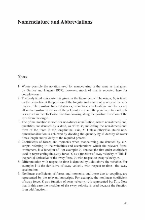
2. The body fixed axis system is given in the figure below. The origin, O, is taken on the centreline at the position of the longitudinal centre of gravity of the sub-marine. The positive linear distances, velocities, accelerations and forces are all in the positive direction of the relevant axes, and the positive rotational val-ues are all in the clockwise direction looking along the positive direction of the axes from the origin.
3. The prime notation is used for non-dimensionalisation, where non-dimensional quantities are denoted by a dash, as with: X′, indicating the non-dimensional form of the force in the longitudinal axis, X. Unless otherwise stated non-dimensionalisation is achieved by dividing the quantity by ½ density of water times length and velocity to the required powers.
4. Coefficients of forces and moments when manoeuvring are denoted by sub-scripts referring to the velocities and accelerations which the relevant force, or moment, is a function of. For example: Yv denotes the first order coefficient used in representing the sway force, Y, as a function of sway velocity, v. This is the partial derivative of the sway force, Y, with respect to sway velocity, v.
5. Differentiation with respect to time is denoted by a dot above the variable. For example: v is the derivative of sway velocity with respect to time—the sway acceleration.
6. Nonlinear coefficients of forces and moments, and those due to coupling, are represented by the relevant subscripts. For example, the nonlinear coefficient of sway force, Y, as a function of sway velocity, v, is represented by: Yv|v|. Note that in this case the modulus of the sway velocity is used because the function is an odd function.

Nomenclature and Abbreviationsxiv
7. Where possible the notation used is that commonly used for the topic being discussed. Thus in some cases the same quantity is defined by different symbols in different chapters.
8. For brevity, where symbols are only used in one location in the text, and are clearly defined there, then these are not always defined in the notation.
Axis system
x
z
x
y
O
O
Symbols
Afrontal Frontal area of sailAm Submarine midships cross-sectional areaAplan Plan area of appendagea Chord of flat plateai, bi, ci, Coefficients used to represent the resistance
of the submarine in the x-axisB Upward force due to the buoyancy (=∇ρg)B Position of centre of buoyancyBF Position of centre of buoyancy of form displacementBG Distance between the centre of buoyancy
and the centre of gravityBGF Distance between the centre of buoyancy
and the centre of gravity corrected for free surfaceBH Position of centre of buoyancy of hydrostatic displacementBM Distance between the centre of buoyancy
and the metacentreBp Propulsor loading coefficientb Span of flat platebg Vertical upward force through the centre of buoyancyCD Non-dimensional drag coefficient at zero angle of attackCDα Non-dimensional slope of drag as a function of angle
of attack
Nomenclature and Abbreviations xv
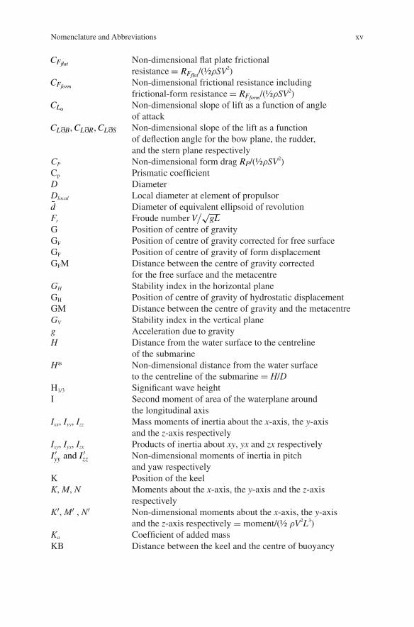
CFflat Non-dimensional flat plate frictional resistance = RFflat/(½ρSV2)
CFform Non-dimensional frictional resistance including frictional-form resistance = RFform/(½ρSV2)
CLα Non-dimensional slope of lift as a function of angle of attack
CLðB,CLðR,CLðS Non-dimensional slope of the lift as a function of deflection angle for the bow plane, the rudder, and the stern plane respectively
CP Non-dimensional form drag RP/(½ρSV2)Cp Prismatic coefficientD DiameterDlocal Local diameter at element of propulsord Diameter of equivalent ellipsoid of revolutionFr Froude number V
/√gL
G Position of centre of gravityGF Position of centre of gravity corrected for free surfaceGF Position of centre of gravity of form displacementGFM Distance between the centre of gravity corrected
for the free surface and the metacentreGH Stability index in the horizontal planeGH Position of centre of gravity of hydrostatic displacementGM Distance between the centre of gravity and the metacentreGV Stability index in the vertical planeg Acceleration due to gravityH Distance from the water surface to the centreline
of the submarineH* Non-dimensional distance from the water surface
to the centreline of the submarine = H/DH1/3 Significant wave heightI Second moment of area of the waterplane around
the longitudinal axisIxx, Iyy, Izz Mass moments of inertia about the x-axis, the y-axis
and the z-axis respectivelyIxy, Iyx, Izx Products of inertia about xy, yx and zx respectivelyI ′yy and I ′zz Non-dimensional moments of inertia in pitch
and yaw respectivelyK Position of the keelK, M, N Moments about the x-axis, the y-axis and the z-axis
respectivelyK′, M′ , N′ Non-dimensional moments about the x-axis, the y-axis
and the z-axis respectively = moment/(½ ρV2L3)Ka Coefficient of added massKB Distance between the keel and the centre of buoyancy

Nomenclature and Abbreviationsxvi
KBF Distance between the keel and the centre of buoyancy of the form displacement
KGF Distance between the keel and the centre of gravity of the form displacement
KGF Distance between the keel and the centre of gravity corrected for free surface
KM Distance between the keel and the metacentreKP Ratio of pressure resistance to friction resistanceK ′δXi
, M ′δXi
, N ′δXi
Non-dimensional coefficient of moment due to the angle of appendage Xi about the x-axis, y-axis and z-axis respectively
K ′∗, M
′∗, N
′∗, Y
′∗, Z
′∗ Non-dimensional roll moment, pitch moment, yaw moment,
sway force, and heave force respectively when the submarine is travelling at steady state with p = q = r = v = w = 0 and no appendage deflection angles
kx, ky, kz Added mass coefficients for motion in the x, y, and z directions respectively
L LengthLA Length of aft bodyLbp Length between perpendicularsLF Length of fore bodyLoa Length overallLPMB Length of parallel middle bodylapp Horizontal coordinate of the centre of pressure,
or centre of added mass, of an appendageM Position of the metacentreMin, Mout In phase and out of phase components respectively
of the measured pitch moment during a PMM testMMEAN Mean pitch moment in wavesM ′
MEAN Non-dimensional mean pitch moment in waves = MMEAN/ρgLDζ
2w
Mm(t), Zm(t) Measured pitch moment and heave force as a function of time
MRAO First order pitch moment response amplitude operatorM ′
RAO Non-dimensional first order pitch moment response amplitude operator = MRAO/ρgL
2DζwMwapp , Mqapp Rate of change of moment about the y-axis on an appendage
as a function of heave velocity and pitch velocity respectively
m Mass of the submarinemadded Added massm′ Non-dimensional mass = m/(½ρL3)mg Vertical downward force through the centre of gravityN Propulsor rate of rotation (revolutions per minute)

Nomenclature and Abbreviations xvii
Nin, Nout In phase and out of phase components respectively of the measured yaw moment during a PMM test
Nvapp , Nrapp Rate of change of moment about the z-axis on an appendage as a function of sway velocity and yaw velocity respectively
n Propulsor rate of rotation (revolutions per second)nf Coefficient defining the fullness of the fore bodyO Position of the originP External vertical force due to grounding or contact with icePE Effective powerPS Shaft powerPT Thrust powerp, q, r Angular velocities about the x-axis, the y-axis and the z-axis
respectivelyp, q, r Angular accelerations about the x-axis, the y-axis and the
z-axis respectivelyp′, q′, r′ Non-dimensional angular velocities about the x-axis, the
y-axis and the z-axis respectively = angular velocity × L/VR Radius of turning circleRcontrol surface Drag of control surfaceRe Reynolds number = VL/νRFflat Friction resistance of a flat plateRFform Frictional resistance including frictional-form resistanceRP Form dragRsailform Form drag of sailRT Total resistancerxf Radius of the section of the fore body at a distance xf
from the rearmost part of the fore bodyS Wetted surface areaSa Plan form area of lifting surfaceShull Wetted surface of submarine hullT Thrust of propulsorT0 Wave modal periodt Thrust deduction fractiont Timeu, v, w Velocities in the x, y and z directions respectivelyu, v, w Accelerations in the x, y and z directions respectivelyu′, v′,w′ Non-dimensional velocities in the x, y and z directions
respectively = velocity/VuaB, uaR, uaS Axial velocity at the bow plane, the rudder, and the stern
plane respectivelyuc Steady state velocity in the x-axis at the set propeller rpm
when the submarine has only velocity in the x-axis and has no control surfaces deflected
V VelocityVa Velocity of advance of the propulsor

Nomenclature and Abbreviationsxviii
VB,VR,VS Velocity at the bow plane, the rudder, and the stern plane respectively
VBeff ,VReff ,VSeff Effective velocity at the bow plane, the rudder, and the stern plane respectively
V* Local axial velocity into the propulsorvR Sway velocity at the rudder (uncorrected for the presence
of the hull)W Downward force due to the mass = Δgw Taylor wake fractionwB, ws Heave velocity at the bow plane and stern plane respectively
(uncorrected for the presence of the hull)X, Y, Z Forces in the x-axis, y-axis and z-axis respectivelyX ′, Y ′, Z ′ Non-dimensional forces in the x-axis, y-axis and z-axis
respectively = force/(½ρV2L2)X ′δXδXi
, Y ′δXi
, Z ′δXi
Non-dimensional coefficient of force due to the angle of appendage Xi in the x-axis, y-axis and z-axis respectively
x, y, z Coordinates in the x-axis, y-axis and z-axis respectivelyxB, yB, zB Coordinates of the centre of buoyancy in the x-axis, y-axis
and z-axis respectivelyxbow, xrudder, xstern x coordinate of the bow plane, the rudder, and the stern
plane respectivelyxCLR x coordinate of the position of the Centre of Lateral
ResistancexCP x coordinate of the position of the Critical Pointxf Distance in the x-direction forward of the rearmost part
of the fore bodyxG, yG, zG Coordinates of the centre of gravity in the x-axis, y-axis
and z-axis respectivelyx′G Non-dimensional x-coordinate of the position of the centre
of gravity = xG/LxNP x coordinate of the position of the Neutral PointYin, Yout In phase and out of phase components respectively
of the measured sway force during a PMM testYr, Yv, Zq, Zw First order coefficients of force as functions of velocities
(q, r, v, and w)Yvapp , Yrapp Rate of change of force in the y-axis on an appendage as a
function of sway velocity, and yaw velocity respectivelyY ′vapp
Contribution of an appendage to the non-dimensional sway added mass coefficient
y0, z0 Amplitude of oscillation in the y-axis and z-axis respectively during PMM tests
Zin, Zout In phase and out of phase components respectively of the measured heave force during a PMM test
Nomenclature and Abbreviations xix
ZMEAN Mean heave force in wavesZ ′MEAN Non-dimensional mean heave force in waves = ZMEAN
/
ρgLζ 2wZRAO First order heave force response amplitude operatorZ ′RAO Non-dimensional first order heave force response amplitude
operator = ZRAO/
ρgL2ζwZwapp , Zqapp Rate of change of force in the z-axis on an appendage
as a function of heave velocity, and pitch velocity respectively
Z ′wapp
Contribution of an appendage to the non-dimensional heave added mass coefficient
α Angle of attackγB, γR, γS Flow straightening effect of the presence of the submarine
hull for the bow plane, the rudder and the stern plane respectively
δ Appendage deflection angleδB, δR, δS Deflection angle of the bow plane, the rudder, and the stern
plane respectivelyδBeff , δReff , δSeff Effective bow plane angle, rudder angle, and stern plane
angle respectivelyδ0 Amplitude of rudder angle oscillation in zig-zag manoeuvreΔ DisplacementΔF Form displacementΔH Hydrostatic displacementζw Wave heightη Ratio of self-propulsion velocity for set value of rpm
to actual velocityηH Hull efficiency: ratio of effective power to thrust powerηO Open water propeller efficiencyηR Relative rotative efficiencyθ Pitch angleθ0, ψ0 Amplitude of oscillation about the y-axis and z-axis
respectively during PMM testsν Kinematic viscosityξhull Hull form factorρ Density of waterτ Trim angleφ Roll angleψ Yaw angle, heading angleψ0 Amplitude of heading angle used for zig-zag manoeuvreω Frequency of oscillation∇ Volume

Nomenclature and Abbreviationsxx
Abbreviations
AMC Australian Maritime College, an Institute of The University of Tasmania
ATT Aft Trim TankCFD Computational Fluid DynamicsCIS Cavitation Inception SpeedCLR Centre of Lateral ResistanceCOTS Commercial Off The ShelfDDD Deep Dive DepthDERA Defence, Evaluation and Research Agency, UKDGA Direction Générale de l’Armement, the French Government
Defence Procurement AgencyDSTO Defence Science and Technology Organisation, AustraliaFSC Free Surface CorrectionFTT Forward Trim TankGRP Glass Reinforced PlasticHPMM Horizontal Planar Motion MechanismITTC International Towing Tank ConferenceLCB Position of the Longitudinal Centre of BuoyancyLCG Position of the Longitudinal Centre of GravityMBT Main Ballast TankMDTF Marine Dynamics Test FacilityMED Maximum Excursion DepthMLD Manoeuvring Limitation DiagramPMB Parallel Middle BodyPMM Planar Motion MechanismQPC Quasi Propulsive CoefficientRANS Reynolds Averaged Navier-Stokesrpm Revolutions Per MinuteSOP Standard Operating ProcedureSSBN Nuclear Powered Ballistic SubmarineSSK Conventionally Powered SubmarineSSN Nuclear Powered Attack SubmarineSSPA Swedish Maritime Consulting OrganisationVPMM Vertical Planar Motion Mechanism

xxi
Author Biography
Prof. Martin Renilson has been working in the field of Ship Hydrodynamics for over 35 years. He established the Ship Hydrodynamics Centre at the Australian Maritime College (AMC) in 1983, and was Director of the Australian Maritime Engineering Cooperative Research Centre in 1992. He started the Department of Naval Architecture & Ocean Engineering at AMC in 1996, which he ran until 2001 when he was appointed Technical Manager, Maritime Platforms & Equipment for DERA/QinetiQ in the UK. In 2007 Professor Renilson returned to Australia and set up his own company, conducting maritime related consulting. He also held a part time chair in hydrodynamics at AMC, now an institute of the University of Tasmania. In 2012 he was appointed inaugural Dean of Maritime Programs at the Higher Colleges of Technology, United Arab Emirates, to start maritime education for the country. He is also an Adjunct Professor in Hydrodynamics at the University of Tasmania, Australia.e-mail: [email protected]

1
Abstract Submarines are very specialised vehicles, and their design is extremely complex. This book deals with only the hydrodynamics aspects of submarines, and a basic knowledge of ship hydrodynamics is assumed. The principles of submarine geometry are outlined in this chapter, covering those terms which are not common to naval architecture, such as: axisymmetric hull; sail; aft body; fore body; control surfaces; casing; and propulsor.
Keywords Axisymmetric body · Submarine geometry · Sail · Propulsor
1.1 General
Submarines are very specialised vehicles, and their design is extremely complex. This book deals only with the hydrodynamics aspects of submarines, and a basic knowledge of ship hydrodynamics is assumed. Readers are referred to texts such as Rawson and Tupper (2001) for information about surface ship concepts.
Although nuclear powered submarines can be much larger than many surface ships, it is traditional to refer to all submarines as “boats” regardless of their size. This convention is retained in this book.
1.2 Geometry
Submarine geometry is fairly straightforward; however there are various terms used which are not common to naval architecture in general. Firstly the hull is usually based on an axisymmetric body: one which is perfectly symmetrical around its longitudinal axis, as shown in Fig. 1.1. Also indicated in Fig. 1.1 are the length, and the diameter of the axisymmetric body.
Chapter 1Introduction
© The Author(s) 2015 M. Renilson, Submarine Hydrodynamics, SpringerBriefs in Applied Sciences and Technology, DOI 10.1007/978-3-319-16184-6_1

2 1 Introduction
For operational purposes it is necessary to add a sail, or bridge fin, to house items such as periscopes, the snorkel and other masts, as shown in Fig. 1.2. This can also be used as a platform to control the boat from when it is on the water sur-face. For consistency, this will be referred to as the sail, throughout this book. The sail generally has a detrimental effect on the hydrodynamic performance of the submarine.
In addition, forward and aft control surfaces are required to control the boat, as discussed in Chap. 3. Details of the hydrodynamic aspects of the design of these control surfaces are given in Chap. 6. For a boat with a conventional cruciform stern the aft control surfaces will include both an upper and a lower rudder, as shown in Fig. 1.2.
Many modern submarines are propelled by a single propulsor located on the longitudinal axis. This is normally located aft of the aft control surfaces, as shown in Fig. 1.3.
Fig. 1.1 Axisymmetric body
Diameter
Length
Fig. 1.2 Submarine geometry
Sail
Diameter
Parallel Middle BodyAft Body ForeBody
Upper rudder
Lower rudder
Fig. 1.3 Common stern configuration
Propulsor
Aft control surfaces
Fig. 1.4 Cross section showing casing
Casing

3
Note that the term “propulsor” is often used as this can refer to either a conventional propeller, or a pumpjet, as discussed in Chap. 5.
Although an axisymmetric shape is good for underwater performance it is difficult to operate on the curved upper part of this when the boat is on the surface, and for this reason many submarines are fitted with an external casing, as shown in Fig. 1.4.
In addition to providing a convenient platform to operate from when on the surface, the casing also provides storage space outside the pressure hull which can be useful for operational purposes.
Reference
Rawson KJ, Tupper EC (2001) Basic ship theory, 5th edn. Butterworth-Heinemann, Boston
1.2 Geometry
5
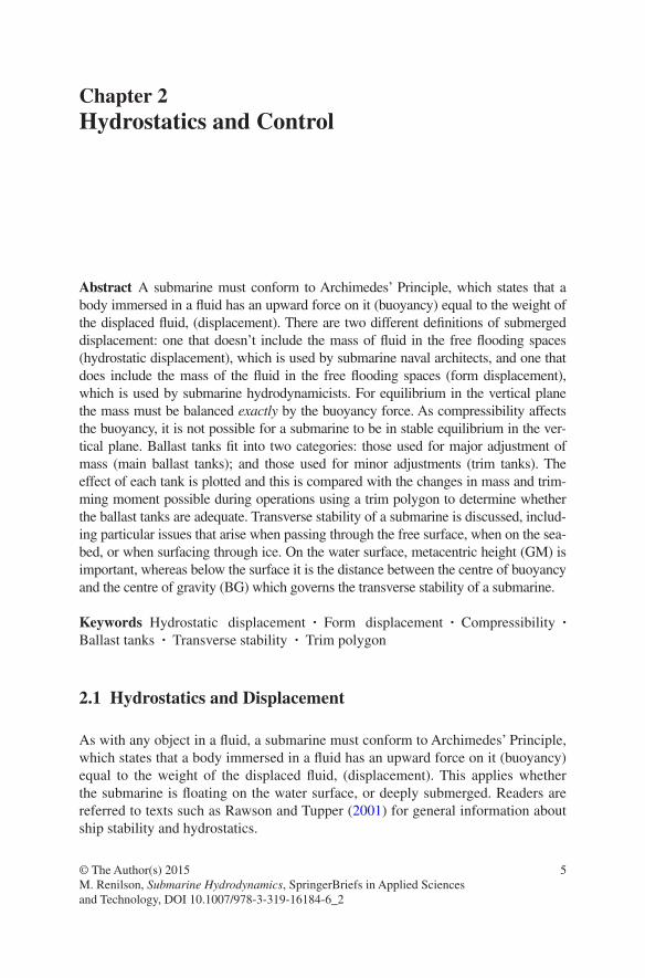
Abstract A submarine must conform to Archimedes’ Principle, which states that a body immersed in a fluid has an upward force on it (buoyancy) equal to the weight of the displaced fluid, (displacement). There are two different definitions of submerged displacement: one that doesn’t include the mass of fluid in the free flooding spaces (hydrostatic displacement), which is used by submarine naval architects, and one that does include the mass of the fluid in the free flooding spaces (form displacement), which is used by submarine hydrodynamicists. For equilibrium in the vertical plane the mass must be balanced exactly by the buoyancy force. As compressibility affects the buoyancy, it is not possible for a submarine to be in stable equilibrium in the ver-tical plane. Ballast tanks fit into two categories: those used for major adjustment of mass (main ballast tanks); and those used for minor adjustments (trim tanks). The effect of each tank is plotted and this is compared with the changes in mass and trim-ming moment possible during operations using a trim polygon to determine whether the ballast tanks are adequate. Transverse stability of a submarine is discussed, includ-ing particular issues that arise when passing through the free surface, when on the sea-bed, or when surfacing through ice. On the water surface, metacentric height (GM) is important, whereas below the surface it is the distance between the centre of buoyancy and the centre of gravity (BG) which governs the transverse stability of a submarine.
Keywords Hydrostatic displacement · Form displacement · Compressibility · Ballast tanks · Transverse stability · Trim polygon
2.1 Hydrostatics and Displacement
As with any object in a fluid, a submarine must conform to Archimedes’ Principle, which states that a body immersed in a fluid has an upward force on it (buoyancy) equal to the weight of the displaced fluid, (displacement). This applies whether the submarine is floating on the water surface, or deeply submerged. Readers are referred to texts such as Rawson and Tupper (2001) for general information about ship stability and hydrostatics.
Chapter 2Hydrostatics and Control
© The Author(s) 2015 M. Renilson, Submarine Hydrodynamics, SpringerBriefs in Applied Sciences and Technology, DOI 10.1007/978-3-319-16184-6_2
6 2 Hydrostatics and Control
When it is floating on the water surface, less of the boat is under the water, and hence the buoyancy and the displacement will be less than when it is submerged.
A key feature of a submarine is its ability to vary its mass, and hence to change from floating on the water surface, to being fully submerged, and vice versa. Therefore, a submarine will have a submerged displacement, for when it is operating under the surface, and a surface displacement for operations on the water surface. It is quite normal to have more than one surfaced displacement, depending on the level of reserve buoyancy required for any given operation. This principle is exactly the same as that for a conventional vessel, which may operate at more than one draught.
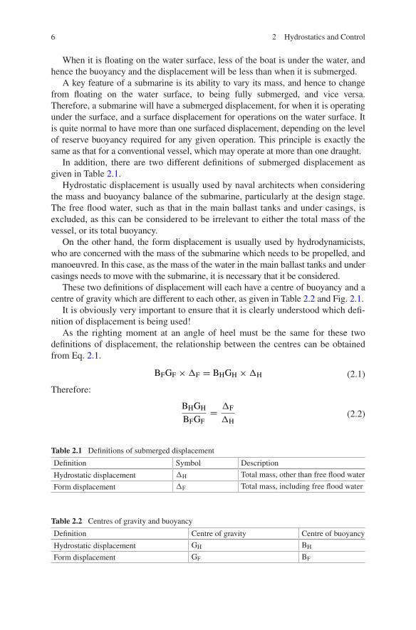
In addition, there are two different definitions of submerged displacement as given in Table 2.1.
Hydrostatic displacement is usually used by naval architects when considering the mass and buoyancy balance of the submarine, particularly at the design stage. The free flood water, such as that in the main ballast tanks and under casings, is excluded, as this can be considered to be irrelevant to either the total mass of the vessel, or its total buoyancy.
On the other hand, the form displacement is usually used by hydrodynamicists, who are concerned with the mass of the submarine which needs to be propelled, and manoeuvred. In this case, as the mass of the water in the main ballast tanks and under casings needs to move with the submarine, it is necessary that it be considered.
These two definitions of displacement will each have a centre of buoyancy and a centre of gravity which are different to each other, as given in Table 2.2 and Fig. 2.1.
It is obviously very important to ensure that it is clearly understood which defi-nition of displacement is being used!
As the righting moment at an angle of heel must be the same for these two definitions of displacement, the relationship between the centres can be obtained from Eq. 2.1.
Therefore:
(2.1)BFGF �F = BHGH �H
(2.2)BHGH
BFGF
=�F
�H
Table 2.1 Definitions of submerged displacement
Definition Symbol Description
Hydrostatic displacement ΔH Total mass, other than free flood water
Form displacement ΔF Total mass, including free flood water
Table 2.2 Centres of gravity and buoyancy
Definition Centre of gravity Centre of buoyancy
Hydrostatic displacement GH BH
Form displacement GF BF

7
2.2 Static Control
2.2.1 Control in the Vertical Plane
The downward force due to the mass multiplied by gravity must be balanced by the upward buoyancy force given by the immersed volume multiplied by the water density and gravity.
Unlike for a surface ship, in the case of a deeply submerged submarine the immersed volume cannot be increased by increasing the vessel’s draught. Thus, for equilibrium in the vertical plane the mass must be balanced exactly by the buoyancy force. Clearly this is difficult, if not impossible to achieve.
To further complicate the issue, the deeper the submarine is operating at, the greater the water pressure acting on it will be, resulting in the hull being com-pressed. This will reduce the immersed volume, and hence the upward buoyancy force. Conversely, if the submarine moves closer to the surface the water pressure acting on it will be less, and hence the immersed volume and the upward buoy-ancy force will be greater. This is illustrated in Fig. 2.2.
The magnitude of this compressibility effect will depend on the submarine structure, however it is important to recognise that many modern submarines are fitted with acoustic tiles, which themselves are compressible, increasing the mag-nitude of this problem.
Thus, the best that can be achieved is for a submarine to be in unstable equilib-rium at a given depth of submergence. A slight upward or downward movement from this position will result in the boat moving away from this initial position.
Further, small changes in sea water density occur in the vertical and horizontal planes, particularly close to coasts. These will also have a significant influence on the ability to control the submarine in the vertical plane.
Fig. 2.1 Centres of gravity and buoyancy
BF
GF
BH
GH
2.2 Static Control

8 2 Hydrostatics and Control
In addition, the mass on board will change during a voyage due to use of consumables and discharge of weapons.
Hence, it is necessary to have the ability to make small changes in mass of the boat very quickly, which is done by a series of ballast tanks, as discussed in Sect. 2.3. Even then, it is very difficult to control a submarine in the vertical plane at zero forward speed, and so it is necessary to make use of hydrodynamic forces, as discussed in Chap. 3.
2.2.2 Transverse Stability
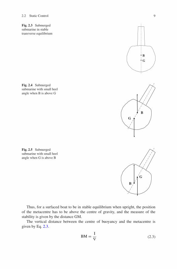
For a submerged submarine to be stable in roll, known as transverse stability, the centre of buoyancy must be above the centre of gravity, as shown in Fig. 2.3. In this case, if the boat is heeled to a small angle, as shown in Fig. 2.4, the hydro-static moment on it will cause it to return to the upright. On the other hand, if the centre of gravity is above the centre of buoyancy, and an external moment causes it to be heeled to a small angle, then the hydrostatic moment will cause it to con-tinue to heel, as shown in Fig. 2.5.
The measure of transverse stability is then given by the distance BG. As noted in Sect. 2.1, for a given submarine this distance will be different depending on whether it is the hydrostatic or form displacement which is being considered. A positive BG value is necessary for a submerged submarine, and is usually easy to achieve, since in many ways the more critical element of transverse stability occurs when surfacing or submerging, as discussed in Sect. 2.5.
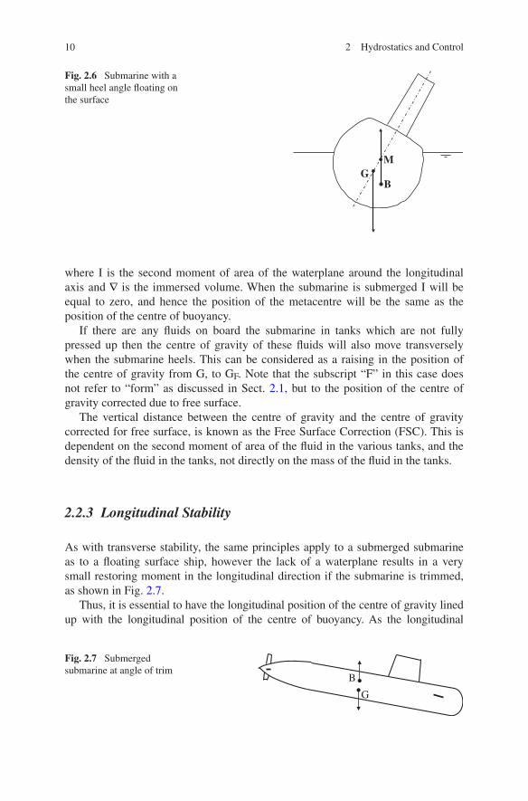
When the submarine is floating on the surface the situation is different. In this case, the centre of buoyancy moves transversely when the boat heels. For small angles the upward force through the centre of buoyancy always acts through the metacentre, designated as “M” in Fig. 2.6.
Fig. 2.2 Effect of compressibility on buoyancy force
Boat in balance
Upward force greater than downward force
Upward force smaller than downward force
9
Thus, for a surfaced boat to be in stable equilibrium when upright, the position of the metacentre has to be above the centre of gravity, and the measure of the stability is given by the distance GM.
The vertical distance between the centre of buoyancy and the metacentre is given by Eq. 2.3.
(2.3)BM =I
∇
Fig. 2.3 Submerged submarine in stable transverse equilibrium
B
G
Fig. 2.4 Submerged submarine with small heel angle when B is above G
B
G
Fig. 2.5 Submerged submarine with small heel angle when G is above B
B
G
2.2 Static Control
10 2 Hydrostatics and Control
where I is the second moment of area of the waterplane around the longitudinal axis and ∇ is the immersed volume. When the submarine is submerged I will be equal to zero, and hence the position of the metacentre will be the same as the position of the centre of buoyancy.
If there are any fluids on board the submarine in tanks which are not fully pressed up then the centre of gravity of these fluids will also move transversely when the submarine heels. This can be considered as a raising in the position of the centre of gravity from G, to GF. Note that the subscript “F” in this case does not refer to “form” as discussed in Sect. 2.1, but to the position of the centre of gravity corrected due to free surface.
The vertical distance between the centre of gravity and the centre of gravity corrected for free surface, is known as the Free Surface Correction (FSC). This is dependent on the second moment of area of the fluid in the various tanks, and the density of the fluid in the tanks, not directly on the mass of the fluid in the tanks.
2.2.3 Longitudinal Stability
As with transverse stability, the same principles apply to a submerged submarine as to a floating surface ship, however the lack of a waterplane results in a very small restoring moment in the longitudinal direction if the submarine is trimmed, as shown in Fig. 2.7.
Thus, it is essential to have the longitudinal position of the centre of gravity lined up with the longitudinal position of the centre of buoyancy. As the longitudinal
Fig. 2.6 Submarine with a small heel angle floating on the surface
BG
M
Fig. 2.7 Submerged submarine at angle of trim
B
G
11
position of the centre of gravity moves during a voyage due to use of consumables, firing of weapons, etc., it is necessary to be able to adjust this by use of ballast tanks, as discussed in Sect. 2.3.
2.3 Ballast Tanks
2.3.1 Categories of Ballast Tanks
Ballast tanks fit into two different categories:
(a) those used for major adjustment of submarine mass to allow it to operate submerged as well as on the surface (main ballast tanks); and
(b) those used for minor adjustments to keep the submarine balanced when submerged (trim and compensation system).
2.3.2 Main Ballast Tanks
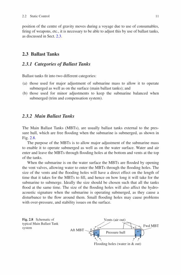
The Main Ballast Tanks (MBTs), are usually ballast tanks external to the pres-sure hull, which are free flooding when the submarine is submerged, as shown in Fig. 2.8.
The purpose of the MBTs is to allow major adjustment of the submarine mass to enable it to operate submerged as well as on the water surface. Water and air enter and leave the MBTs through flooding holes at the bottom and vents at the top of the tanks.
When the submarine is on the water surface the MBTs are flooded by opening the vent valves, allowing water to enter the MBTs through the flooding holes. The size of the vents and the flooding holes will have a direct effect on the length of time that it takes for the MBTs to fill, and hence on how long it will take for the submarine to submerge. Ideally the size should be chosen such that all the tanks flood at the same time. The size of the flooding holes will also affect the hydro-acoustic signature when the submarine is operating submerged, as they cause a disturbance to the flow around them. Small flooding holes may cause problems with over-pressure, and stability issues on the surface.
Fig. 2.8 Schematic of typical Main Ballast Tank system
Pressure hullAft MBT
Fwd MBT
Vents (air out)
Flooding holes (water in & out)
2.2 Static Control
12 2 Hydrostatics and Control
2.3.3 Trim and Compensation Ballast Tanks
During operations the mass and longitudinal centre of gravity of a submarine will change due to use of consumables including fuel, and weapons discharge. In addi-tion, changes in seawater density, hull compressibility and surface suction when operating close to the surface will all result in the need to be able to make small changes to the submarine mass and longitudinal centre of gravity.
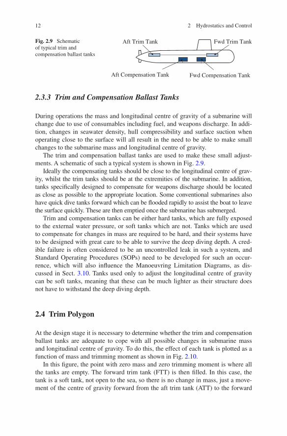
The trim and compensation ballast tanks are used to make these small adjust-ments. A schematic of such a typical system is shown in Fig. 2.9.
Ideally the compensating tanks should be close to the longitudinal centre of grav-ity, whilst the trim tanks should be at the extremities of the submarine. In addition, tanks specifically designed to compensate for weapons discharge should be located as close as possible to the appropriate location. Some conventional submarines also have quick dive tanks forward which can be flooded rapidly to assist the boat to leave the surface quickly. These are then emptied once the submarine has submerged.
Trim and compensation tanks can be either hard tanks, which are fully exposed to the external water pressure, or soft tanks which are not. Tanks which are used to compensate for changes in mass are required to be hard, and their systems have to be designed with great care to be able to survive the deep diving depth. A cred-ible failure is often considered to be an uncontrolled leak in such a system, and Standard Operating Procedures (SOPs) need to be developed for such an occur-rence, which will also influence the Manoeuvring Limitation Diagrams, as dis-cussed in Sect. 3.10. Tanks used only to adjust the longitudinal centre of gravity can be soft tanks, meaning that these can be much lighter as their structure does not have to withstand the deep diving depth.
2.4 Trim Polygon
At the design stage it is necessary to determine whether the trim and compensation ballast tanks are adequate to cope with all possible changes in submarine mass and longitudinal centre of gravity. To do this, the effect of each tank is plotted as a function of mass and trimming moment as shown in Fig. 2.10.
In this figure, the point with zero mass and zero trimming moment is where all the tanks are empty. The forward trim tank (FTT) is then filled. In this case, the tank is a soft tank, not open to the sea, so there is no change in mass, just a move-ment of the centre of gravity forward from the aft trim tank (ATT) to the forward
Fig. 2.9 Schematic of typical trim and compensation ballast tanks
Aft Trim Tank Fwd Trim Tank
Aft Compensation Tank Fwd Compensation Tank

13
trim tank. Thus, the effect is a forward trimming moment with no change in mass. This is shown by a horizontal line.
Next, the forward compensation tank is filled. As this is open to the sea, and filled from sea water, the effect of this will be an increase in mass. As this is slightly forward of the longitudinal centre of gravity there will also be a small for-ward trimming moment as shown.
This is continued until all the trim and compensation ballast tanks are full, as seen at the top of the graph.
Then, the FTT is emptied, and the effect of this can be seen as an aft trim-ming moment. Note that this line will be exactly the same as the line representing the filling of the FTT. The remaining tanks are then emptied in sequence, and the results plotted, until all the tanks are emptied and the line has returned to the point with zero mass and zero trimming moment.
This then results in a polygon, which indicates the maximum effect that can be achieved by the trim and compensation ballast tank system.
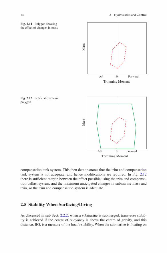
A similar polygon is then prepared to represent all the possible changes in mass and trimming moment due to use of consumables, including fuel, and weapons discharge. The effects of compressibility and surface suction can also be incorpo-rated into this polygon, as can the anticipated in-service growth. A very simplified version of the polygon is shown in Fig. 2.11.
To ensure that the maximum change in mass and trimming moment that can be caused by factors such as changes in consumables etc. can be adequately compen-sated for by the trim and compensation tank system, these two polygons are plot-ted together, as shown in Fig. 2.12.
If any part of the dashed line falls outside the solid line then it is possible that changes to the submarine mass cannot be compensated for by the trim and
Fig. 2.10 Polygon showing the effect of trim and compensation ballast tanks
Trimming Moment
Mas
s
0 ForwardAft
FTT full
Fwd comptank full
Aft comptank full
ATT fullFTT empty
Fwd comptank empty
Aft comptank empty
2.4 Trim Polygon
14 2 Hydrostatics and Control
compensation tank system. This then demonstrates that the trim and compensation tank system is not adequate, and hence modifications are required. In Fig. 2.12 there is sufficient margin between the effect possible using the trim and compensa-tion ballast system, and the maximum anticipated changes in submarine mass and trim, so the trim and compensation system is adequate.
2.5 Stability When Surfacing/Diving
As discussed in sub Sect. 2.2.2, when a submarine is submerged, transverse stabil-ity is achieved if the centre of buoyancy is above the centre of gravity, and this distance, BG, is a measure of the boat’s stability. When the submarine is floating on
Fig. 2.11 Polygon showing the effect of changes in mass
Trimming MomentM
ass
0 ForwardAft
Fig. 2.12 Schematic of trim polygon
Mas
s
Trimming Moment
Aft 0 Forward
15
the water surface the centre of buoyancy moves transversely as a function of heel angle. For small angles this acts through the metacentre, M. Thus, the measure of stability is then the distance that the metacentre is above the centre of gravity, GM.
As a submarine transitions from floating on the water surface to fully sub-merged its vertical centres of both buoyancy and gravity will vary, due to a change in immersion of the hull, and the change in mass in the ballast tanks. In addition, the second moment of the waterplane, I, will vary during this process. This will also significantly affect the position of the metacentre, M, Eq. 2.3.
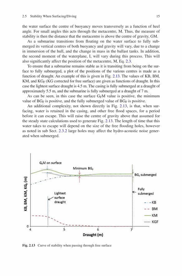
To ensure that a submarine remains stable as it is transiting from being on the sur-face to fully submerged, a plot of the positions of the various centres is made as a function of draught. An example of this is given in Fig. 2.13. The values of KB, BM, KM, and KGF (KG corrected for free surface) are given as functions of draught. In this case the lightest surface draught is 4.5 m. The casing is fully submerged at a draught of approximately 5.5 m, and the submarine is fully submerged at a draught of 7 m.
As can be seen, in this case the surface GFM value is positive, the minimum value of BGF is positive, and the fully submerged value of BGF is positive.
An additional complexity, not shown directly in Fig. 2.13, is that, when sur-facing, water is retained in the casing, and other free flood spaces, for a period before it can escape. This will raise the centre of gravity above that assumed for the steady state calculations used to generate Fig. 2.13. The length of time that this water takes to escape will depend on the size of the free flooding holes, however as noted in sub Sect. 2.3.2 large holes may affect the hydro-acoustic noise gener-ated when submerged.
Fig. 2.13 Curve of stability when passing through free surface
2.5 Stability When Surfacing/Diving
16 2 Hydrostatics and Control
2.6 Stability When Bottoming
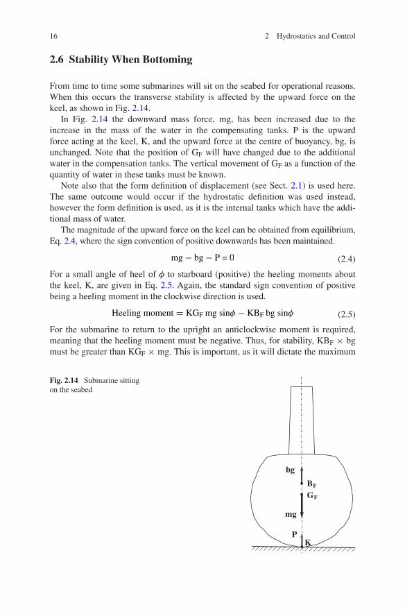
From time to time some submarines will sit on the seabed for operational reasons. When this occurs the transverse stability is affected by the upward force on the keel, as shown in Fig. 2.14.
In Fig. 2.14 the downward mass force, mg, has been increased due to the increase in the mass of the water in the compensating tanks. P is the upward force acting at the keel, K, and the upward force at the centre of buoyancy, bg, is unchanged. Note that the position of GF will have changed due to the additional water in the compensation tanks. The vertical movement of GF as a function of the quantity of water in these tanks must be known.
Note also that the form definition of displacement (see Sect. 2.1) is used here. The same outcome would occur if the hydrostatic definition was used instead, however the form definition is used, as it is the internal tanks which have the addi-tional mass of water.
The magnitude of the upward force on the keel can be obtained from equilibrium, Eq. 2.4, where the sign convention of positive downwards has been maintained.
For a small angle of heel of φ to starboard (positive) the heeling moments about the keel, K, are given in Eq. 2.5. Again, the standard sign convention of positive being a heeling moment in the clockwise direction is used.
For the submarine to return to the upright an anticlockwise moment is required, meaning that the heeling moment must be negative. Thus, for stability, KBF × bg must be greater than KGF × mg. This is important, as it will dictate the maximum
(2.4)mg− bg− P = 0
(2.5)Heeling moment = KGF mg sinφ − KBF bg sinφ
Fig. 2.14 Submarine sitting on the seabed
BF
GF
KP
mg
bg
17
amount of water that can be added to the compensating tanks whilst remaining stable. If these are located low in the boat, then there may not be a limit to the amount of water without affecting stability, however if these are high, then it may be necessary to set a limit of the amount of water in the compensating tanks in this condition, to maintain transverse stability.
2.7 Stability When Surfacing Through Ice
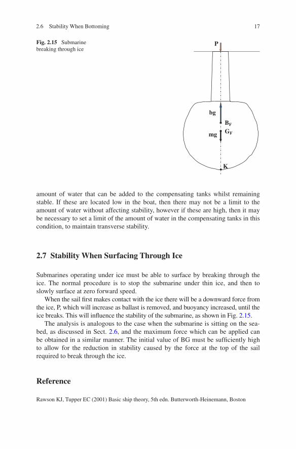
Submarines operating under ice must be able to surface by breaking through the ice. The normal procedure is to stop the submarine under thin ice, and then to slowly surface at zero forward speed.
When the sail first makes contact with the ice there will be a downward force from the ice, P, which will increase as ballast is removed, and buoyancy increased, until the ice breaks. This will influence the stability of the submarine, as shown in Fig. 2.15.
The analysis is analogous to the case when the submarine is sitting on the sea-bed, as discussed in Sect. 2.6, and the maximum force which can be applied can be obtained in a similar manner. The initial value of BG must be sufficiently high to allow for the reduction in stability caused by the force at the top of the sail required to break through the ice.
Reference
Rawson KJ, Tupper EC (2001) Basic ship theory, 5th edn. Butterworth-Heinemann, Boston
Fig. 2.15 Submarine breaking through ice
BF
GF
K
mg
bg
P
2.6 Stability When Bottoming
19
Abstract The equations of motion for submarine manoeuvring are presented and discussed together with a non-linear coefficient based approach for determining the forces and moments on the submarine. Means of determining the coefficients using model tests, including a rotating arm and a planar motion mechanism, are detailed. In addition, the use of Computational Fluid Dynamics; and empirical techniques for determining the manoeuvring coefficients are discussed. Empirical equations for determining the manoeuvring coefficients are presented, and the results compared to published results from experiments. Issues associated with manoeuvring in the horizontal and vertical planes are explained, including: sta-bility in the horizontal plane; the Pivot Point; heel during a turn, including snap roll; the effect of the sail, including the stern dipping effect; the Centre of Lateral Resistance; stability in the vertical plane; the Neutral Point; and the Critical Point, including the effect of speed, and issues at very low speed. Manoeuvring close to the surface, including surface suction, is discussed. Suggested criteria for stability in the horizontal and vertical planes, along with rudder and hydroplane effective-ness are given. The concept of Manoeuvring Limitation Diagrams and associated Standard Operating Procedures in event of a credible failure is presented. Free running model experiments and manoeuvring trials, including submarine definitive manoeuvres and submarine trials procedures are discussed.
Keywords Manoeuvring coefficients · Neutral Point · Critical Point · Surface suction · Criteria for stability · Manoeuvring Limitation Diagrams
3.1 Introduction
The basic concepts behind the manoeuvring of a submarine are very similar to that of a surface ship. The main differences between a study of submarine manoeu-vring and that of surface ship manoeuvring are that a submarine can manoeuvre in all six degrees of freedom, but is very unlikely to be required to manoeuvre whilst going astern.
Chapter 3Manoeuvring and Control
© The Author(s) 2015 M. Renilson, Submarine Hydrodynamics, SpringerBriefs in Applied Sciences and Technology, DOI 10.1007/978-3-319-16184-6_3
20 3 Manoeuvring and Control
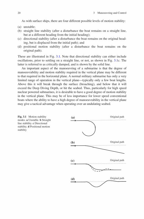
As with surface ships, there are four different possible levels of motion stability:
(a) unstable;(b) straight line stability (after a disturbance the boat remains on a straight line,
but at a different heading from the initial heading);(c) directional stability (after a disturbance the boat remains on the original head-
ing, but is displaced from the initial path); and(d) positional motion stability (after a disturbance the boat remains on the
original path).
These are illustrated in Fig. 3.1. Note that directional stability can either include oscillations, prior to settling on a straight line, or not, as shown in Fig. 3.1c. The latter is referred to as critically damped, and is shown by the solid line.
An important aspect of the manoeuvring of a submarine is that the degree of manoeuvrability and motion stability required in the vertical plane may be different to that required in the horizontal plane. A normal military submarine has only a very limited range of operation in the vertical plane—typically only a few boat lengths. Above this it will break through the surface (broaching), and below that it will exceed the Deep Diving Depth, or hit the seabed. Thus, particularly for high speed nuclear powered submarines, it is desirable to have a good degree of motion stability in the vertical plane. This may be of less importance for lower speed conventional boats where the ability to have a high degree of manoeuvrability in the vertical plane may give a tactical advantage when operating over an undulating seabed.
Fig. 3.1 Motion stability modes. a Unstable. b Straight line stability. c Directional stability. d Positional motion stability
Original path
Original path
Original path
Original path
(a)
(b)
(c)
(d)

21
Hence, an important aspect for the submarine designer at an early stage in the design is to determine the level of manoeuvrability and motion stability required in each plane. Recommended values are given in Sect. 3.9.
Another important point is that with the controls fixed the degree of motion stability possible in the vertical plane is different to that in the horizontal plane. In the horizontal plane, the greatest possible level of motion stability with the controls fixed is straight line stability. With this level of stability, after being disturbed by a small deflection a submarine will return to a straight line motion, but not in the same direction as prior to the disturbance, as shown in Fig. 3.1b. To achieve the same direction it is necessary to have operating controls.
On the other hand, it is possible for a submarine to have directional stability in the vertical plane. With this level of stability, after being disturbed by a small deflection a submarine will return to the same direction. This is shown in Fig. 3.1c. This is possible because of the influence of the hydrostatic force, discussed in Chap. 2, which provides a pitch restoring moment.
3.2 Equations of Motion
The equations of motion for a submarine are similar to those for a surface ship, however they include all six degrees of freedom. For a submarine it is normal to take the origin as the longitudinal centre of gravity (LCG), rather than mid-ships, as this simplifies the equations, and for a submarine this position is fixed (unlike for a surface ship). The axis system used is shown in the notation. Note that the origin is on the centreline, which is where the transverse centre of grav-ity is assumed to be. Positive directions are along the positive axes, and positive rotations are clockwise as seen from the origin looking along the positive direction of the axes.
The notation is given in Table 3.1, and in the notation section.
Table 3.1 Notation Position Velocity Force/moment
Surge x u X
Sway y v Y
Heave z w Z
Roll φ p K
Pitch θ q M
Yaw ψ r N
Appendage δ
Propulsor n
3.1 Introduction
22 3 Manoeuvring and Control
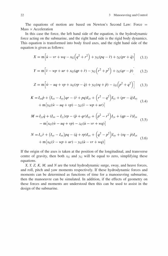
The equations of motion are based on Newton’s Second Law: Force = Mass × Acceleration
In this case the force, the left hand side of the equation, is the hydrodynamic force acting on the submarine, and the right hand side is the rigid body dynamics. This equation is transformed into body fixed axes, and the right hand side of the equation is given as follows:
If the origin of the axes is taken at the position of the longitudinal, and transverse centre of gravity, then both xG and yG will be equal to zero, simplifying these equations.
X, Y, Z, K, M, and N are the total hydrodynamic surge, sway, and heave forces, and roll, pitch and yaw moments respectively. If these hydrodynamic forces and moments can be determined as functions of time for a manoeuvring submarine, then the manoeuvre can be simulated. In addition, if the effects of geometry on these forces and moments are understood then this can be used to assist in the design of the submarine.
(3.1)X = m[
u− vr + wq − xG
(
q2 + r2)
+ yG(pq − r)+ zG(pr + q)
]
(3.2)Y = m[
v− wp+ ur + xG(qp+ r)− yG
(
r2 + p2)
+ zG(qr − p)
]
(3.3)Z = m[
w− uq + vp+ xG(rp− q)+ yG(rq + p)− zG
(
p2 + q2)]
(3.4)K = Ixxp+
(
Ixx − Iyy)
qr − (r + pq)Izx +(
r2 − q2)
Iyz + (pr − q)Ixy
+m[
yG(w− uq + vp)− zG(v− wp+ ur)]
(3.5)M = Iyyq + (Ixx − Izz)rp− (p+ qr)Ixy +
(
p2 − r2)
Izx + (qp− r)Iyx
−m[
xG(w− uq + vp)− zG(u− vr + wq)]
(3.6)N = Izzr +
(
Iyy − Ixx)
pq − (q + rp)Iyx +(
q2 − p2)
Ixy + (rq − p)Izx
+m[
xG(v− wp+ ur)− yG(u− vr + wq)]
23
3.3 Hydrodynamic Forces—Steady State Assumption
One approach to determining the hydrodynamic forces and moments on a manoeuvring submarine is to assume that at any point in time these forces and moments are functions of the motions (velocities and accelerations), propeller rpm, and appendage angles, at that point in time. This is a similar approach to that used for surface ships.
As with surface ships, the relationship between each motion variable and the resultant force or moment can be represented by a mathematical model compris-ing a series of coefficients. The resulting forces and moments due to each of these are then added to give the total force or moment on the submarine at that point in time. The choice of which coefficients, and hence which mathematical model, to use will depend on experience. It is normal for a single mathematical model to be used by a given organisation to represent different submarines. Once the math-ematical model representing the forces and moments has been selected, different submarines, or changes to the shape of a given submarine, can be represented by changing the values of the individual coefficients.
It is important to recognise that as different organisations may use different mathematical models it is not necessarily possible to compare the values of coef-ficients between different organisations. Also, as improvements in understand-ing are achieved, and the mathematical model updated, care needs to be taken to ensure that legacy coefficient sets are retained for past submarines.
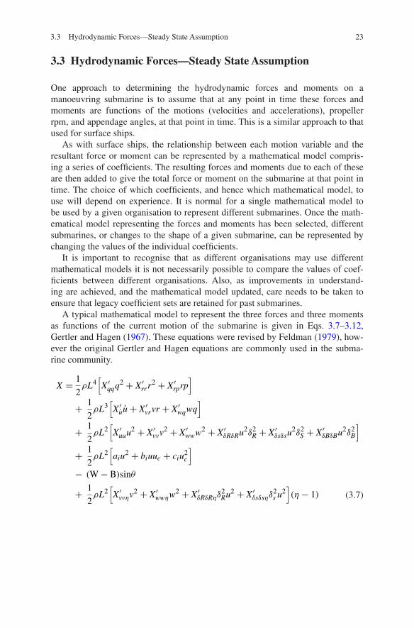
A typical mathematical model to represent the three forces and three moments as functions of the current motion of the submarine is given in Eqs. 3.7–3.12, Gertler and Hagen (1967). These equations were revised by Feldman (1979), how-ever the original Gertler and Hagen equations are commonly used in the subma-rine community.
(3.7)
X =1
2ρL4
[
X ′qqq
2 + X ′rrr
2 + X ′rprp
]
+1
2ρL3
[
X ′uu+ X ′
vrvr + X ′wqwq
]
+1
2ρL2
[
X ′uuu
2 + X ′vvv
2 + X ′www
2 + X ′δRδRu
2δ2R + X ′δsδsu
2δ2S + X ′δBδBu
2δ2B
]
+1
2ρL2
[
aiu2 + biuuc + ciu
2c
]
− (W− B)sinθ
+1
2ρL2
[
X ′vvηv
2 + X ′wwηw
2 + X ′δRδRηδ
2Ru
2 + X ′δsδsηδ
2s u
2]
(η − 1)
3.3 Hydrodynamic Forces—Steady State Assumption

24 3 Manoeuvring and Control
(3.8)
Y =1
2ρL4
[
Y ′r r + Y ′
pp+ Y ′p|p|p|p| + Y ′
pqpq + Y ′qrqr
]
+1
2ρL3
[
Y ′v v+ Y ′
vqvq + Y ′wpwp+ Y ′
wrwr]
+1
2ρL3
[
Y ′rur + Y ′
pup+ Y ′|r|δRu|r|δR + Y ′
v|r|v
|v|
∣
∣
∣
∣
(
v2 + w2)
12
∣
∣
∣
∣
|r|]
+1
2ρL2
[
Y ′∗u
2 + Y ′vuv+ Y ′
v|v|v
∣
∣
∣
∣
(
v2 + w2)
12
∣
∣
∣
∣
+ Y ′vwvw+ Y ′
δRu2δR
]
+ (W− B)cosθ sinφ
+1
2ρL3Y ′
rηur(η − 1)
+1
2ρL2
[
Y ′vηuv+ Y ′
v|v|ηv
∣
∣
∣
∣
(
v2 + w2)
12
∣
∣
∣
∣
+ Y ′δRηu
2δR
]
(η − 1)
(3.9)
Z =1
2ρL4
[
Z ′qq + Z ′
ppp2 + Z ′
rrr2 + Z ′
rprp]
+1
2ρL3
[
Z ′ww+ Z ′
vrvr + Z ′vpvp + Z ′
quq + Z ′|q|δsu|q|δs
]
+1
2ρL3
[
Z ′w|q|
w
|w|
∣
∣
∣
∣
(
v2 + w2)
12
∣
∣
∣
∣
|q|]
+1
2ρL2
[
Z ′∗u
2 + Z ′vuv + Z ′
wuw+ Z ′w|w|w
∣
∣
∣
∣
(
v2 + w2)
12
∣
∣
∣
∣
]
+1
2ρL2
[
Z ′|w|u|w| + Z ′
ww
∣
∣
∣
∣
w(
v2 + w2)
12
∣
∣
∣
∣
]
+1
2ρL2
[
Z ′vvv
2 + Z ′δsu
2δs + Z ′δBu
2δB
]
+ (W− B)cosθ cosφ
+1
2ρL3Z ′
qηuq(η − 1)
+1
2ρL2
[
Z ′wηuw+ Z ′
w|w|ηw
∣
∣
∣
∣
(
v2 + w2)
12
∣
∣
∣
∣
+ Z ′δsηδsu
2
]
(η − 1)
(3.10)
K =1
2ρL5
[
K ′pp+ K ′
r r + K ′qrqr + K ′
pqpq + K ′p|p|p|p|
]
+1
2ρL4
[
K ′pup+ K ′
rur + K ′v v + K ′
vqvq + K ′wpwp+ K ′
wrwr]
+1
2ρL3
[
K ′∗u
2 + K ′vuv + K ′
v|v|v
∣
∣
∣
∣
(
v2 + w2)
12
∣
∣
∣
∣
+ K ′vwvw+ K ′
δRu2δR
]
+ (yGW− yBB)cosθ cosφ − (zGW− zBB)cosθ sinφ
+1
2ρL3K ′
∗ηu2(η − 1)
25
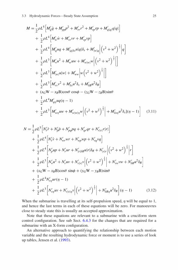
When the submarine is travelling at its self-propulsion speed, η will be equal to 1, and hence the last terms in each of these equations will be zero. For manoeuvres close to steady state this is usually an accepted approximation.
Note that these equations are relevant to a submarine with a cruciform stern control configuration. See sub Sect. 6.4.3 for the changes that are required for a submarine with an X-form configuration.
An alternative approach to quantifying the relationship between each motion variable and the resulting hydrodynamic force or moment is to use a series of look up tables, Jensen et al. (1993).
(3.11)
M =1
2ρL5
[
M ′qq +M ′
ppp2 +M ′
rrr2 +M ′
rprp+M ′q|q|q|q|
]
+1
2ρL4
[
M ′ww+M ′
vrvr +M ′vpvp
]
+1
2ρL4
[
M ′quq +M ′
|q|δsu|q|δs +M ′|w|q
∣
∣
∣
∣
(
v2 + w2)
12
∣
∣
∣
∣
q
]
+1
2ρL3
[
M ′∗u
2 +M ′wuw+M ′
w|w|w
∣
∣
∣
∣
(
v2 + w2)
12
∣
∣
∣
∣
]
+1
2ρL3
[
M ′|w|u|w| +M ′
ww
∣
∣
∣
∣
w(
v2 + w2)
12
∣
∣
∣
∣
]
+1
2ρL3
[
M ′vvv
2 +M ′δsu
2δs +M ′δBu
2δB
]
+ (xGW− xBB)cosθ cosφ − (zGW− zBB)sinθ
+1
2ρL4M ′
qηuq(η − 1)
+1
2ρL3
[
M ′wηuw+M ′
w|w|ηw
∣
∣
∣
∣
(
v2 + w2)
12
∣
∣
∣
∣
+M ′δsηu
2δs](η − 1)
]
(3.12)
N =1
2ρL5
[
N ′r r + N ′
pp+ N ′pqpq + N ′
qrqr + N ′r|r|r|r|
]
+1
2ρL4
[
N ′v v+ N ′
wrwr + N ′wpwp+ N ′
vqvq]
+1
2ρL4
[
N ′pup+ N ′
rur + N ′|r|δRu|r|δR + N ′
|v|r
∣
∣
∣
∣
(
v2 + w2)
12
∣
∣
∣
∣
r
]
+1
2ρL3
[
N ′∗u
2 + N ′vuv + N ′
v|v|v
∣
∣
∣
∣
(
v2 + w2)
12
∣
∣
∣
∣
+ N ′vwvw+ N ′
δRu2δR
]
+ (xGW− xBB)cosθ sinφ + (yGW− yBB)sinθ
+1
2ρL4N ′
rηur(η − 1)
+1
2ρL3
[
N ′vηuv+ N ′
v|v|ηv
∣
∣
∣
∣
(
v2 + w2)
12
∣
∣
∣
∣
+ N ′δRηu
2δR
]
(η − 1)
3.3 Hydrodynamic Forces—Steady State Assumption
26 3 Manoeuvring and Control
In principle this makes it easier to ‘fit’ measured data as there is complete free-dom as to the form of the function, and it is not necessary to force the data to fit a particular representation using a predetermined expression. This approach can be particularly useful for some relationships, where the function of the force or moment, in terms of the motion parameter, is not a clearly determined smooth curve.
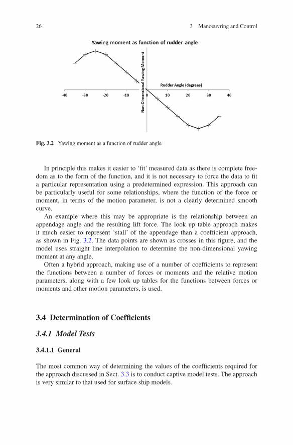
An example where this may be appropriate is the relationship between an appendage angle and the resulting lift force. The look up table approach makes it much easier to represent ‘stall’ of the appendage than a coefficient approach, as shown in Fig. 3.2. The data points are shown as crosses in this figure, and the model uses straight line interpolation to determine the non-dimensional yawing moment at any angle.
Often a hybrid approach, making use of a number of coefficients to represent the functions between a number of forces or moments and the relative motion parameters, along with a few look up tables for the functions between forces or moments and other motion parameters, is used.
3.4 Determination of Coefficients
3.4.1 Model Tests
3.4.1.1 General
The most common way of determining the values of the coefficients required for the approach discussed in Sect. 3.3 is to conduct captive model tests. The approach is very similar to that used for surface ship models.
Fig. 3.2 Yawing moment as a function of rudder angle

27
Normally fairly large models are used (5–6 m long) as even at such a large scale the appendages are actually quite small, with low local Reynolds num-bers. In addition, as scale effects on the shedding of vortices are not fully under-stood, the generally accepted procedure is to use as large a model as possible and to neglect scale effects. Turbulence stimulation is normally fitted to the hull and appendages.
As a deeply submerged submarine does not interact with the surface it is not necessary to conduct captive model experiments at the correct Froude number. Thus, it is only Reynolds number that is of importance.
In principle, tests can be conducted in either water, or air, in a towing tank or a water/wind tunnel. A common procedure is to test in a large towing tank, with the model supported from the carriage using struts as shown in Fig. 3.3.
When testing in a towing tank it is important to recognise the presence of the water free surface. This means that the speed needs to be limited to prevent waves occurring, with the resulting Froude number effects. Most facilities have a com-mon speed that they always test their submarine models at, to give consistency. For example, in the QinetiQ facility at Haslar, UK, the normal test speed is 10 ft per second, which has been used for historical reasons. This, together with a standard turbulence stimulation method, and a similar sized model, means that any scale effects etc. will be consistent for all tests—an important aspect of tank testing.
The effect of the support struts needs to be considered. Although the hydrody-namic forces are measured inside the model, and hence the forces on the struts are not included in the measurements, the presence of the struts can influence the flow around the model. For this reason the model is tested either inverted, or on its side, depending on which coefficients are being investigated.
It is possible to use a sting type mount, as shown in Fig. 3.4, however this gen-erally means that the propulsor cannot be included. As the propulsor has a signifi-cant influence on the flow over the stern of the submarine (see Chap. 4) care needs to be taken with this approach.
The approach used for captive model testing is to confine the model to a given motion, and then to measure the resulting forces.
Fig. 3.3 Typical set up for captive model tests in a towing tank
3.4 Determination of Coefficients

28 3 Manoeuvring and Control
3.4.1.2 Tests in Translation (Sway/Heave)
To obtain the values of the coefficients which represent the forces and moments as functions of sway velocity, such as Yv, Nv, etc., the model is tested on its side with the sway velocity being generated by adjusting the angle of the model in the verti-cal plane. This avoids the need for the struts to be at an angle to the flow, as would be required if the model were rotated in the horizontal plane. This minimises the hydrodynamic disturbance that they create. However, as most towing tanks are wider than they are deep this does have the disadvantage of increasing the effec-tive blockage, compared to adjusting the angle in the horizontal plane. Note that this technique will not work if the effect of the presence of the free surface on manoeuvring in the horizontal plane is being investigated—see Sect. 3.8. For this case it is necessary to use a sting type mount (Fig. 3.4) and adjust the angle of the model in the horizontal plane.
To obtain the values of the coefficients which represent the forces and moments as functions of heave velocity, such as Zw, Mw, etc., the model is tested inverted with the heave velocity being generated by adjusting the angle of the model in the vertical plane. Again, this avoids the need for the struts to be at an angle to the flow.
A schematic of the typical results from such an experiment, where the non-dimensional side force (Y′) is plotted as a function of the non-dimensional sway velocity (v′) is given in Fig. 3.5.
In this case, with the propeller revolutions set to the self-propulsion speed, the hydrodynamic side force is represented by Eq. 3.13, which is simplified from Eq. 3.8.
In Eq. 3.13 there are three unknown terms which can be obtained from this experi-ment: Y ′
∗, Y′v, and Y ′
v|v|. Y′∗ is due to an asymmetry—the results not passing through
Y′ = 0 at v′ = 0. The remaining two coefficients are obtained from a “fit” to the data, with Y ′
v representing the linear characteristic of the data (dominant at low val-ues of v′) and Y ′
v|v| representing the non-linear characteristic. Note that the results
(3.13)Y =1
2ρL2
[
Y ′∗u
2 + Y ′vuv+ Y ′
v|v|v|v|]
Fig. 3.4 Set up for captive model tests using a sting support (taken from Renilson et al. 2011)

29
in Fig. 3.5 are skew symmetric, hence the need for an “odd” term, such as the v|v| term, rather than v2. An alternative would be to use v3, which also provides skew symmetry. However, as hydrodynamic forces tend to be proportional to veloc-ity squared, the v|v| term is often preferred, as in the original work of Gertler and Hagen (1967).
The values of the coefficients which represent the forces and moments as func-tions of appendage angles can be obtained by setting the relevant appendages to the required angles. However, Reynolds number effects can influence the lift and drag on the appendages, as the model scale Reynolds number will be much lower than the full scale value. Hence care has to be taken when interpreting the results. In addition, the appendages operate in the model hull’s boundary layer, which is much larger at model scale than full scale, due to Reynolds number effects, and hence this may also influence the results.
The cross coupling effects between yaw or heave velocity and appendage angles can also be obtained, as can the effect of propulsor rpm on the forces and moments due to the appendage angles. Again, care needs to be taken with scale effects due to testing at the wrong Reynolds number.
3.4.1.3 Rotating Arm
As with surface ship models, to obtain the values of the coefficients which repre-sent the forces and moments as functions of yaw velocity, it is necessary to test the models in rotation, using a rotating arm. This is done in the horizontal plane, and the model is tested inverted, as shown in Fig. 3.6.
The rotating arm can also be used to obtain the values of the coefficients which represent the forces and moments as functions of pitch velocity, and this is done in the horizontal plane, with the model tested on its side.
The arm is fitted with a sub-carriage, as shown in Fig. 3.6, which makes it pos-sible to test a different radii, and hence different values of q (model on side) or r (model inverted).
Fig. 3.5 Schematic of results from a translation test
3.4 Determination of Coefficients

30 3 Manoeuvring and Control
Of course, as with surface ship captive model tests, the rotating arm can be used to obtain the values of the coefficients which represent the forces and moments as functions of yaw and pitch velocity by carrying out cross plots. It can also be used to obtain the values of cross coefficients. A sketch of the results from a rotating arm is given in Fig. 3.7. In this case the model is inverted, and being tested at a range of values of r′. The non-dimensional moment N′ has been plotted as a function of r′ for a range of values of v′.
However, a major difficulty with the rotating arm is that it is not possible to test at small values of q′, or r′, which would require very large radii (q′, r′ = 0 is a straight line). This is shown in Fig. 3.7. In the figure the experimentally obtained points are joined by a dotted line across r′ = 0 where experiments are not possible. The linear coefficient is the gradient of the line at r′ = 0 and the difficulty in obtaining this can be seen.
In this case, when v = 0 the hydrodynamic yaw moment is represented by Eq. 3.14 which is simplified from Eq. 3.12.
Fig. 3.7 Schematic of results from rotating arm
Central pivot
Rotating arm
Sub-carriage Towing strut
Support strut
Submarine model
Counterbalance mass
Fig. 3.6 Typical set up for captive model tests using a rotating arm
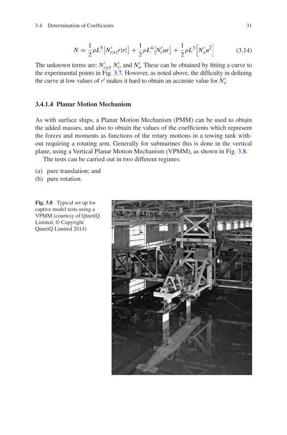
31
The unknown terms are: N ′r|r|, N
′r, and N ′
∗. These can be obtained by fitting a curve to the experimental points in Fig. 3.7. However, as noted above, the difficulty in defining the curve at low values of r′ makes it hard to obtain an accurate value for N ′
r.
3.4.1.4 Planar Motion Mechanism
As with surface ships, a Planar Motion Mechanism (PMM) can be used to obtain the added masses, and also to obtain the values of the coefficients which represent the forces and moments as functions of the rotary motions in a towing tank with-out requiring a rotating arm. Generally for submarines this is done in the vertical plane, using a Vertical Planar Motion Mechanism (VPMM), as shown in Fig. 3.8.
The tests can be carried out in two different regimes:
(a) pure translation; and(b) pure rotation.
(3.14)N =1
2ρL5
[
N ′r|r|r|r|
]
+1
2ρL4
[
N ′rur
]
+1
2ρL3
[
N ′∗u
2]
Fig. 3.8 Typical set up for captive model tests using a VPMM (courtesy of QinetiQ Limited, © Copyright QinetiQ Limited 2014)
3.4 Determination of Coefficients
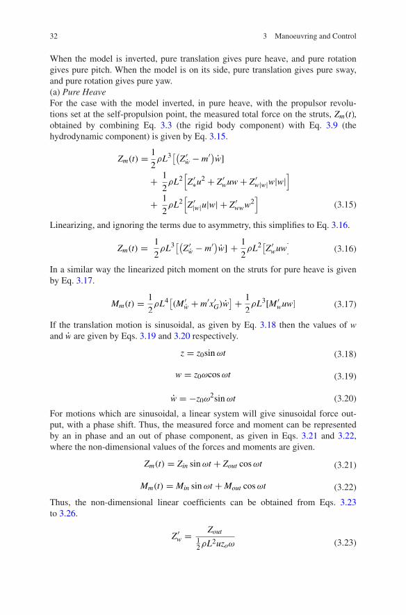
32 3 Manoeuvring and Control
When the model is inverted, pure translation gives pure heave, and pure rotation gives pure pitch. When the model is on its side, pure translation gives pure sway, and pure rotation gives pure yaw.(a) Pure HeaveFor the case with the model inverted, in pure heave, with the propulsor revolu-tions set at the self-propulsion point, the measured total force on the struts, Zm(t), obtained by combining Eq. 3.3 (the rigid body component) with Eq. 3.9 (the hydrodynamic component) is given by Eq. 3.15.
Linearizing, and ignoring the terms due to asymmetry, this simplifies to Eq. 3.16.
In a similar way the linearized pitch moment on the struts for pure heave is given by Eq. 3.17.
If the translation motion is sinusoidal, as given by Eq. 3.18 then the values of w and w are given by Eqs. 3.19 and 3.20 respectively.
For motions which are sinusoidal, a linear system will give sinusoidal force out-put, with a phase shift. Thus, the measured force and moment can be represented by an in phase and an out of phase component, as given in Eqs. 3.21 and 3.22, where the non-dimensional values of the forces and moments are given.
Thus, the non-dimensional linear coefficients can be obtained from Eqs. 3.23 to 3.26.
(3.15)
Zm(t) =1
2ρL3
[(
Z ′w − m′)w]
+1
2ρL2
[
Z ′∗u
2 + Z ′wuw+ Z ′
w|w|w|w|]
+1
2ρL2
[
Z ′|w|u|w| + Z ′
www2]
(3.16)Zm(t) =1
2ρL3
[(
Z ′w − m′)w] +
1
2ρL2
[
Z ′wuw
]
(3.17)Mm(t) =1
2ρL4
[
(M ′w + m′x′G)w
]
+1
2ρL3[M ′
wuw]
(3.18)z = z0sinωt
(3.19)w = z0ωcosωt
(3.20)w = −z0ω2sinωt
(3.21)Zm(t) = Zin sinωt + Zout cosωt
(3.22)Mm(t) = Min sinωt +Mout cosωt
(3.23)Z ′w =
Zout12ρL2uzoω

33
The coefficients determined in this way are frequency dependent, and so it may be necessary to extrapolate to zero frequency to obtain the steady state values which are used in Eqs. 3.7–3.12. For deeply submerged submarine models this is often not required, but should be considered if appropriate.(b) Pure PitchFor pure pitch, with the model inverted, the motion is given by Eqs. 3.27–3.29.
The coefficients can be obtained from Eqs. 3.30 to 3.33.
(c) Pure SwayFor pure sway, with the model on its side, the coefficients can be obtained from Eqs. 3.34 to 3.37.
(3.24)(Z ′w − m′) = −
Zin12ρL3zoω2
(3.25)M ′w =
Mout
12ρL3uz0ω
(3.26)(M ′w − m′x′G) = −
Min
12ρL4zoω2
(3.27)θ = θ0sinωt
(3.28)q = θ0ωcos ωt
(3.29)q = −θ0ω2sin ωt
(3.30)(Z ′q + m′) =
Zout12ρL3uθ0ω
(3.31)(Z ′q + m′x′G) = −
Zin12ρL4θ0ω2
(3.32)(M ′q − m′x′G) =
Mout
12ρL4uθ0ω
(3.33)(M ′q − I ′yy) = −
Min
12ρL5θ0ω2
(3.34)Y ′v =
Yout12ρL2uy0ω
3.4 Determination of Coefficients

34 3 Manoeuvring and Control
(d) Pure YawFor pure yaw, with the model on its side, the coefficients can be obtained from Eqs. 3.38 to 3.41.
In the submarine design process the VPMM is usually used initially to determine the linear coefficients, which are those that affect the straight line stability of the submarine (in both the horizontal and vertical planes). This is used to make any refinements to the shape (if possible) and to determine the required size of the appendages. Once the design has moved to the next stage further tests are con-ducted in both the towing tank and the rotating arm facility.
A detailed description specifically for submarines using a VPMM is given in Booth and Bishop (1973).
3.4.1.5 Marine Dynamics Test Facility
An alternative approach to the PMM is to use a single mechanism to provide motion in all six degrees of freedom. Such a device was developed by the National Research Council, Canada, known as a Marine Dynamics Test Facility (MDTF)
(3.35)(Y ′v − m′) = −
Yin12ρL3y0ω2
(3.36)N ′v =
Nout
12ρL3uy0ω
(3.37)(N ′v − m′x′G) = −
Nin
12ρL4y0ω2
(3.38)(Y ′r − m′) =
Yout12ρL3uψ0ω
(3.39)(Y ′r − m′x′G) = −
Yin12ρL4ψ0ω2
(3.40)(N ′r − m′x′G) =
Nout
12ρL4uψ0ω
(3.41)(N ′r − I ′zz) = −
Nin
12ρL5ψ0ω2
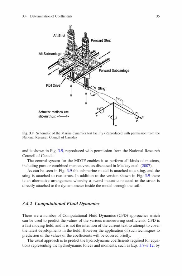
35
and is shown in Fig. 3.9, reproduced with permission from the National Research Council of Canada.
The control system for the MDTF enables it to perform all kinds of motions, including pure or combined manoeuvres, as discussed in Mackay et al. (2007).
As can be seen in Fig. 3.9 the submarine model is attached to a sting, and the sting is attached to two struts. In addition to the version shown in Fig. 3.9 there is an alternative arrangement whereby a sword mount connected to the struts is directly attached to the dynamometer inside the model through the sail.
3.4.2 Computational Fluid Dynamics
There are a number of Computational Fluid Dynamics (CFD) approaches which can be used to predict the values of the various manoeuvring coefficients. CFD is a fast moving field, and it is not the intention of the current text to attempt to cover the latest developments in the field. However the application of such techniques to prediction of the values of the coefficients will be covered briefly.
The usual approach is to predict the hydrodynamic coefficients required for equa-tions representing the hydrodynamic forces and moments, such as Eqs. 3.7–3.12, by
Fig. 3.9 Schematic of the Marine dynamics test facility (Reproduced with permission from the National Research Council of Canada)
3.4 Determination of Coefficients
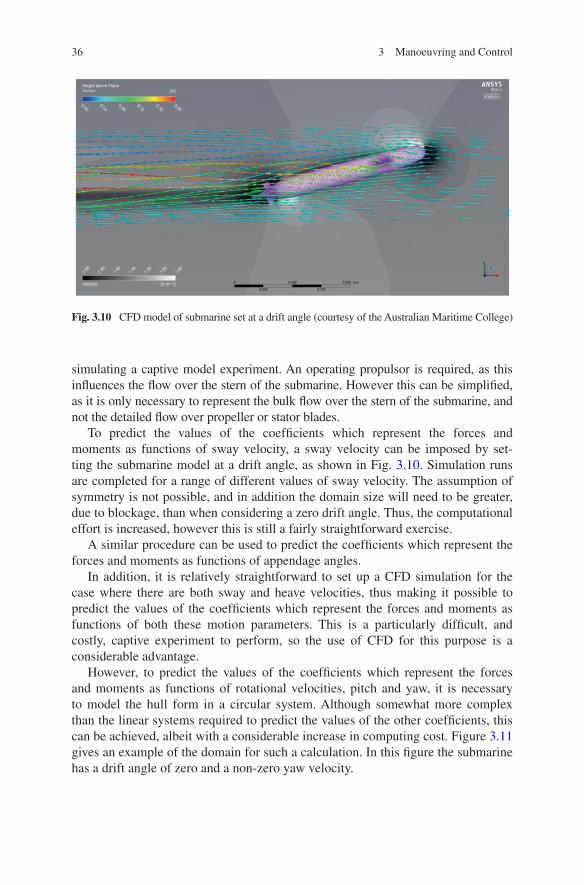
36 3 Manoeuvring and Control
simulating a captive model experiment. An operating propulsor is required, as this influences the flow over the stern of the submarine. However this can be simplified, as it is only necessary to represent the bulk flow over the stern of the submarine, and not the detailed flow over propeller or stator blades.
To predict the values of the coefficients which represent the forces and moments as functions of sway velocity, a sway velocity can be imposed by set-ting the submarine model at a drift angle, as shown in Fig. 3.10. Simulation runs are completed for a range of different values of sway velocity. The assumption of symmetry is not possible, and in addition the domain size will need to be greater, due to blockage, than when considering a zero drift angle. Thus, the computational effort is increased, however this is still a fairly straightforward exercise.
A similar procedure can be used to predict the coefficients which represent the forces and moments as functions of appendage angles.
In addition, it is relatively straightforward to set up a CFD simulation for the case where there are both sway and heave velocities, thus making it possible to predict the values of the coefficients which represent the forces and moments as functions of both these motion parameters. This is a particularly difficult, and costly, captive experiment to perform, so the use of CFD for this purpose is a considerable advantage.
However, to predict the values of the coefficients which represent the forces and moments as functions of rotational velocities, pitch and yaw, it is necessary to model the hull form in a circular system. Although somewhat more complex than the linear systems required to predict the values of the other coefficients, this can be achieved, albeit with a considerable increase in computing cost. Figure 3.11 gives an example of the domain for such a calculation. In this figure the submarine has a drift angle of zero and a non-zero yaw velocity.
Fig. 3.10 CFD model of submarine set at a drift angle (courtesy of the Australian Maritime College)
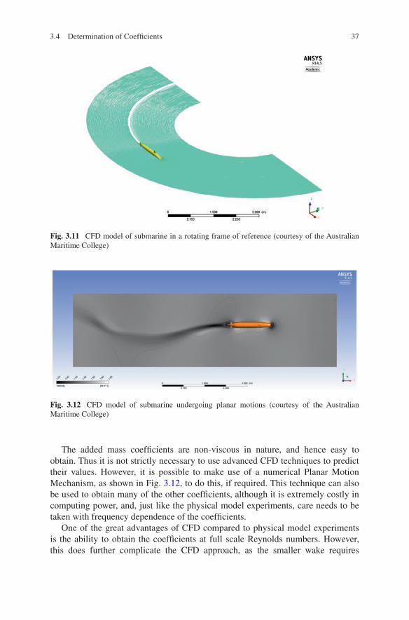
37
The added mass coefficients are non-viscous in nature, and hence easy to obtain. Thus it is not strictly necessary to use advanced CFD techniques to predict their values. However, it is possible to make use of a numerical Planar Motion Mechanism, as shown in Fig. 3.12, to do this, if required. This technique can also be used to obtain many of the other coefficients, although it is extremely costly in computing power, and, just like the physical model experiments, care needs to be taken with frequency dependence of the coefficients.
One of the great advantages of CFD compared to physical model experiments is the ability to obtain the coefficients at full scale Reynolds numbers. However, this does further complicate the CFD approach, as the smaller wake requires
Fig. 3.11 CFD model of submarine in a rotating frame of reference (courtesy of the Australian Maritime College)
Fig. 3.12 CFD model of submarine undergoing planar motions (courtesy of the Australian Maritime College)
3.4 Determination of Coefficients

38 3 Manoeuvring and Control
a greater grid size. In addition, it is not possible to compare the results from the CFD predictions with those from captive model experiments.
Another advantage of the CFD compared to physical model experiments is the ability to carry out the predictions without the presence of the support struts which are necessary for the captive physical model tests. It is also possible to make use of CFD to predict the effects of the support struts on the physical model, and hence to correct the results of physical model tests for them.
CFD can be used to determine the forces and moments on individual com-ponents of the submarine, such as the sail, and also to easily conduct flow visu-alisation. Both can be very valuable, particularly if the results show unusual or unexpected trends.
One of the big difficulties with using CFD techniques to predict the perfor-mance of a submarine is that such techniques are advancing at a very high rate. This means that the results from a prediction made today, using current tech-niques, will differ from those for the same hull form made only a few years ago. This is quite different to most physical model tests, which have been refined over a period of years and now remain essentially constant, at least for routine tests used to predict full scale performance. This means that it is difficult to develop empiri-cal correlation factors, which will always be necessary to bridge the gap between even the best prediction techniques, and full scale performance.
Thus, it is important for any hydrodynamics organisation to carefully record the numerical techniques used, and preferably not to continuously change these, but only to do so in a well-documented step form.
3.4.3 Approximation Techniques
3.4.3.1 General
In the early design stage it is desirable to be able to estimate the manoeuvring characteristics of a submarine. This will be necessary long before either advanced CFD modelling or physical model experiments are commissioned. This is needed to determine the size of the appendages, for example, to give the desirable level of straight line stability. When this is required simple approximation methods for predicting the values of the linear coefficients are needed.
It is known that these approximation methods are not necessary very accurate, as discussed in Jones et al. (2002). This means that the results from these initial predictions should be treated with care, and confirmed by either CFD or physical model experiments. It is unrealistic to expect these approximation methods to be able to accurately predict the non-linear coefficients.
Unlike the situation for surface ships, there is not a large library of publically available experimental data to draw upon.
One approach is to first determine the coefficients for the unappended hull, and then add the influence of the appendages, including the sail. Interaction between

39
the hull and the appendages may need to be considered, although for a preliminary estimation this may not be required.
Note that, in general, the contribution to many of the manoeuvring coefficients from the hull is quite low, with that from the sail and hydroplanes being much larger.
3.4.3.2 Hull
For a purely axisymmetric body, the side force/yawing moment due to sway motion/sway acceleration will be identical to the vertical force/pitching moment due to heave motion/heave acceleration, and the side force/yawing moment due to yaw motion/acceleration will be identical to the heave force/pitching moment due to pitch motion/acceleration. This leads to Eqs. 3.42–3.49. Note that due to the sign convention, the coefficients: N ′
v and M ′w; and N ′
v and M ′w will have opposite signs.
For an axisymmetric body all the coupling between roll moment and motions in the horizontal and vertical planes will be zero. In addition, a number of the linear terms will be zero, due to symmetry, as given in Eq. 3.50.
In ideal flow the pressure distribution along the length of a symmetrical hull in pure sway or pure heave is illustrated schematically in Fig. 3.13. As can be seen, there will be no net side force as the pressure over the forward half of the body will be identical to the pressure over the aft half of the body. However there will
(3.42)Y ′v = Z ′
w
(3.43)Y ′v = Z ′
w
(3.44)N ′v = −M ′
w
(3.45)N ′v = −M ′
w
(3.46)Y ′r = Z ′
q
(3.47)Y ′r = Z ′
q
(3.48)N ′r = M ′
q
(3.49)N ′r = M ′
q
(3.50)Y ′p = Y ′
p = Y ′∗ = Z ′
∗ = Z ′v = M ′
∗ = N ′r = N ′
p = N ′p = N ′
∗ = 0
3.4 Determination of Coefficients
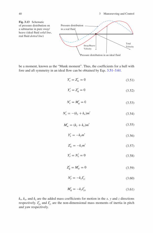
40 3 Manoeuvring and Control
be a moment, known as the “Munk moment”. Thus, the coefficients for a hull with fore and aft symmetry in an ideal flow can be obtained by Eqs. 3.51–3.61.
kx, ky, and kz are the added mass coefficients for motion in the x, y and z directions respectively. I ′yy and I ′zz are the non-dimensional mass moments of inertia in pitch and yaw respectively.
(3.51)Y ′v = Z ′
w = 0
(3.52)Y ′r = Z ′
q = 0
(3.53)N ′r = M ′
q = 0
(3.54)N ′v = −(ky + kx)m
′
(3.55)M ′w = (kz + kx)m
′
(3.56)Y ′v = −kym
′
(3.57)Z ′w = −kzm
′
(3.58)Y ′r = N ′
v = 0
(3.59)Z ′q = M ′
w = 0
(3.60)N ′r = −kzI
′zz
(3.61)M ′q = −kyI
′yy
Fig. 3.13 Schematic of pressure distribution on a submarine in pure sway/heave (ideal fluid solid line, real fluid dotted line)
Pressure distribution in an ideal fluid
Sway/Heave Velocity
Total Velocity
Pressure distribution in a real fluid
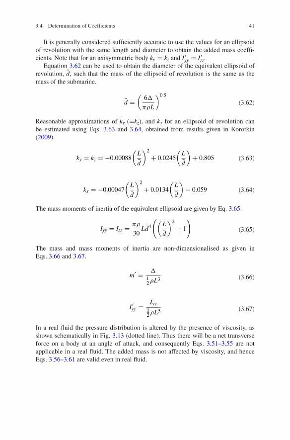
41
It is generally considered sufficiently accurate to use the values for an ellipsoid of revolution with the same length and diameter to obtain the added mass coeffi-cients. Note that for an axisymmetric body ky = kz and I ′yy = I ′zz.
Equation 3.62 can be used to obtain the diameter of the equivalent ellipsoid of revolution, d, such that the mass of the ellipsoid of revolution is the same as the mass of the submarine.
Reasonable approximations of ky (=kz), and kx for an ellipsoid of revolution can be estimated using Eqs. 3.63 and 3.64, obtained from results given in Korotkin (2009).
The mass moments of inertia of the equivalent ellipsoid are given by Eq. 3.65.
The mass and mass moments of inertia are non-dimensionalised as given in Eqs. 3.66 and 3.67.
In a real fluid the pressure distribution is altered by the presence of viscosity, as shown schematically in Fig. 3.13 (dotted line). Thus there will be a net transverse force on a body at an angle of attack, and consequently Eqs. 3.51–3.55 are not applicable in a real fluid. The added mass is not affected by viscosity, and hence Eqs. 3.56–3.61 are valid even in real fluid.
(3.62)d =(
6�
πρL
)0.5
(3.63)ky = kz = −0.00088
(
L
d
)2
+ 0.0245
(
L
d
)
+ 0.805
(3.64)kx = −0.00047
(
L
d
)2
+ 0.0134
(
L
d
)
− 0.059
(3.65)Iyy = Izz =πρ
30Ld4
(
(
L
d
)2
+ 1
)
(3.66)m′ =�
12ρL3
(3.67)I ′yy =Iyy
12ρL5
3.4 Determination of Coefficients
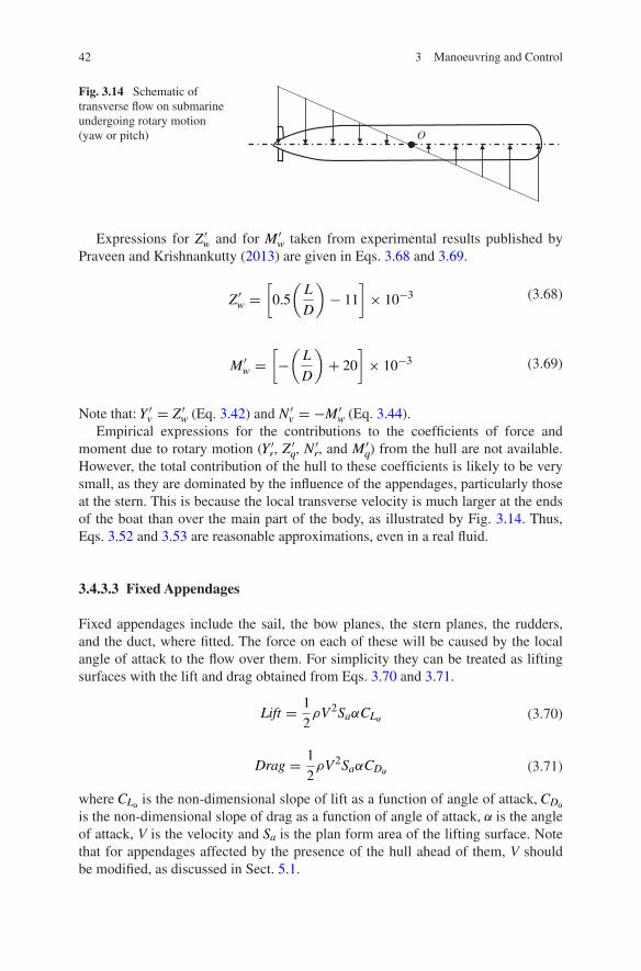
42 3 Manoeuvring and Control
Expressions for Z ′w and for M ′
w taken from experimental results published by Praveen and Krishnankutty (2013) are given in Eqs. 3.68 and 3.69.
Note that: Y ′v = Z ′
w (Eq. 3.42) and N ′v = −M ′
w (Eq. 3.44).Empirical expressions for the contributions to the coefficients of force and
moment due to rotary motion (Y ′r, Z
′q, N
′r, and M ′
q) from the hull are not available. However, the total contribution of the hull to these coefficients is likely to be very small, as they are dominated by the influence of the appendages, particularly those at the stern. This is because the local transverse velocity is much larger at the ends of the boat than over the main part of the body, as illustrated by Fig. 3.14. Thus, Eqs. 3.52 and 3.53 are reasonable approximations, even in a real fluid.
3.4.3.3 Fixed Appendages
Fixed appendages include the sail, the bow planes, the stern planes, the rudders, and the duct, where fitted. The force on each of these will be caused by the local angle of attack to the flow over them. For simplicity they can be treated as lifting surfaces with the lift and drag obtained from Eqs. 3.70 and 3.71.
where CLα is the non-dimensional slope of lift as a function of angle of attack, CDα is the non-dimensional slope of drag as a function of angle of attack, α is the angle of attack, V is the velocity and Sa is the plan form area of the lifting surface. Note that for appendages affected by the presence of the hull ahead of them, V should be modified, as discussed in Sect. 5.1.
(3.68)Z ′w =
[
0.5
(
L
D
)
− 11
]
× 10−3
(3.69)M ′w =
[
−(
L
D
)
+ 20
]
× 10−3
(3.70)Lift =1
2ρV2SaαCLα
(3.71)Drag =1
2ρV2SaαCDα
Fig. 3.14 Schematic of transverse flow on submarine undergoing rotary motion (yaw or pitch) O
43
The transverse force on the body is given by Eq. 3.72.
For horizontal motions this translates into the rate of change of side force as a function of sway velocity, Yvapp, and for vertical motions into the rate of change of vertical force as a function of heave velocity, Zwapp
, in Eqs. 3.73 and 3.74.
CD is the non-dimensional drag at zero angle of attack. Note that Eqs. 3.73 and 3.74 are dimensional. These can be non-dimensionalised in the usual way, based on the length squared of the submarine, as described in the notation.
In each case it is assumed that the lift slope is that generating lift in the desired direction. In other words, for Eq. 3.73 the appendages of interest are the sail and the rudder (fixed), and the relevant lift slopes are used, and for Eq. 3.74 the appendages of interest are the bow and stern hydroplanes (fixed). If a stern config-uration other than a cruciform one is used, then the components of the lift slopes in the relative directions are required. Note also that if a duct is fitted then the forces due to this in the relevant plane should be included.
Thus, to obtain the contribution of the appendages to the manoeuvring coef-ficients, Yv and Zw, it is necessary to know the lift slopes and the drag at zero lift of these appendages. Various empirical methods exist for predicting these in the absence of experimental or numerical data, including those given by references such as: Abbott and von Doenhoff (1960), Molland and Turnock (2007).
It is not intended to repeat all these various empirical methods here, however it should be noted that as the appendages (particularly those at the stern) contribute significantly to the manoeuvring coefficients it is important to be able to predict the lift slopes on these as accurately as possible. Organisations with experience with particular designs of appendages should take advantage of data for these append-ages, which may be proprietary, and it is recommended that such information be validated wherever possible using either model experiments or advanced CFD.
Note also that care needs to be taken when estimating the lift slope for stern appendages, as these are influenced by the presence of the hull ahead of them, and they may operate in decelerating flow due to the half tail cone angle. This is dis-cussed more fully in Mackay (2001, 2003).
The contribution of each appendage to the moment coefficients is given in Eqs. 3.75 and 3.76 by making use of the lever from the origin to the centre of pres-sure of the appendage.
(3.72)Transverse force = Lift cosα + Drag sinα
(3.73)Yvapp = −1
2ρVSa
(
CLα + CD
)
(3.74)Zwapp = −1
2ρVSa
(
CLα + CD
)
(3.75)Nvapp = lapp × Yvapp
(3.76)Mwapp = −lapp × Zwapp
3.4 Determination of Coefficients
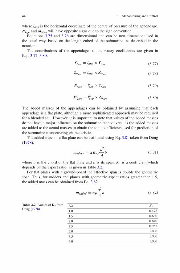
44 3 Manoeuvring and Control
where lapp is the horizontal coordinate of the centre of pressure of the appendage. Nvapp and Mwapp
will have opposite signs due to the sign convention.Equations 3.75 and 3.76 are dimensional and can be non-dimensionalised in
the usual way, based on the length cubed of the submarine, as described in the notation.
The contributions of the appendages to the rotary coefficients are given in Eqs. 3.77–3.80.
The added masses of the appendages can be obtained by assuming that each appendage is a flat plate, although a more sophisticated approach may be required for a blended sail. However, it is important to note that values of the added masses do not have a major influence on the submarine manoeuvres, as the added masses are added to the actual masses to obtain the total coefficients used for prediction of the submarine manoeuvring characteristics.
The added mass of a flat plate can be estimated using Eq. 3.81 taken from Dong (1978).
where a is the chord of the flat plate and b is its span. Ka is a coefficient which depends on the aspect ratio, as given in Table 3.2.
For flat plates with a ground-board the effective span is double the geometric span. Thus, for rudders and planes with geometric aspect ratios greater than 1.5, the added mass can be obtained from Eq. 3.82.
(3.77)Yrapp = lapp × Yvapp
(3.78)Zqapp = lapp × Zwapp
(3.79)Nrapp = l2app × Yvapp
(3.80)Mqapp = l2app × Zwapp
(3.81)madded = πKaρa2
4b
(3.82)madded = πρa2
4b
Table 3.2 Values of Ka from Dong (1978)
b/a Ka
1.0 0.478
1.5 0.680
2.0 0.840
2.5 0.953
3.0 1.000
3.5 1.000
4.0 1.000

45
If alternative methods are available for predicting the added mass they can be used to obtain madded for the appendages.
The contributions of the appendage to the values of the linear sway and heave added mass coefficients are given by Eqs. 3.83 and 3.84.
Where the values of madded used are for the appropriate direction–the sail and rudders contribute to the value for Y ′
vapp and the hydroplanes to the values for Z ′
wapp.
The contributions of the appendages to the other coefficients are given in Eqs. 3.85–3.90 where lapp is the horizontal coordinate of the centre of added mass of the appendage.
3.4.3.4 Propeller
An open propeller will generate a side force when it is at an angle to the flow. This side force will contribute to the manoeuvring coefficients in the same way as a fixed fin located at the longitudinal position of the propeller.
Thus, in order to calculate the contribution of the propeller to the manoeuvring coefficients, it is necessary to know the rate of change of side force as a function of inflow angle (analogous to the lift slope for a fixed fin).
Although some data exists for aircraft propellers (see for example: Ribner 1943) it is not clear how applicable this is to modern submarine propellers. Thus, unless more accurate data is known it may not be possible to predict the effect of an open propeller on the manoeuvring coefficients.
(3.83)Y ′vapp
= −madded
12ρL3
(3.84)Z ′wapp
= −madded
12ρL3
(3.85)N ′vapp
=lapp × Y ′
vapp
L
(3.86)M ′wapp
= −lapp × Z ′
wapp
L
(3.87)Y ′rapp
=lapp × Y ′
vapp
L
(3.88)Z ′qapp
=lapp × Z ′
wapp
L
(3.89)N ′rapp
=l2app × Y ′
vapp
L2
(3.90)M ′qapp
=l2app × Z ′
wapp
L2
3.4 Determination of Coefficients

46 3 Manoeuvring and Control
3.4.3.5 Control Surfaces
The effect of control surfaces on the forces and moments on the submarine can be modelled using linear coefficients, as given in Eqs. 3.8–3.12. The values of these coefficients can be estimated using Eqs. 3.91–3.96 if the lift slope of the active part of the control surface, CLδ, is known. The subscripts “B”, “R” and “S” refer to the bow planes, the rudder and the stern planes respectively. Note that if a stern form other than a cruciform one is used then these coefficients will differ, as discussed in Sect. 6.4.
where VR, VB, and VS are the local velocities at the rudder, the bow planes and the stern planes respectively. Although the local velocity at the bow planes is likely to be very close to the velocity of the submarine, the local velocity at the rudder and stern planes will be influenced by the presence of the hull and the propulsor (see Sect. 5.1).
3.4.3.6 Predictions for Suboff
The above method was applied to the DARPA standard submarine hull form, Suboff. Details of this hull form are given by Groves et al. (1989) and Roddy (1990). The principal particulars of this model are given in Table 3.3. Note that
(3.91)YδR =1
2ρVRCLδR
(3.92)NδR =1
2ρVRxrudderCLδR
(3.93)ZδB = −1
2ρVBCLδB
(3.94)MδB = −1
2ρVBxbowCLδB
(3.95)ZδS = −1
2ρVSCLδS
(3.96)MδS = −1
2ρVSxsternCLδS
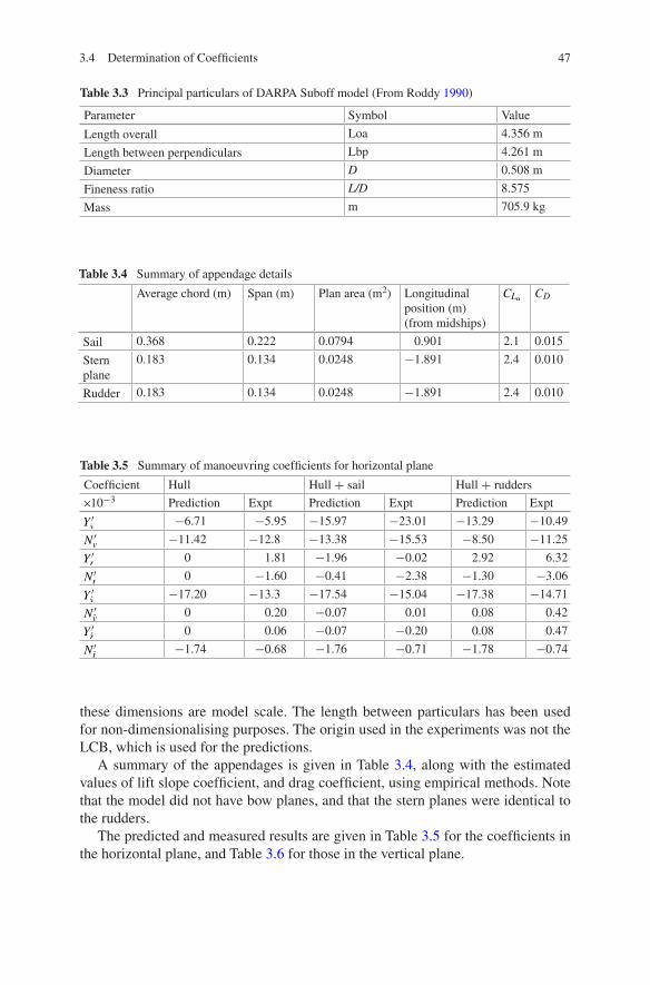
47
these dimensions are model scale. The length between particulars has been used for non-dimensionalising purposes. The origin used in the experiments was not the LCB, which is used for the predictions.
A summary of the appendages is given in Table 3.4, along with the estimated values of lift slope coefficient, and drag coefficient, using empirical methods. Note that the model did not have bow planes, and that the stern planes were identical to the rudders.
The predicted and measured results are given in Table 3.5 for the coefficients in the horizontal plane, and Table 3.6 for those in the vertical plane.
Table 3.3 Principal particulars of DARPA Suboff model (From Roddy 1990)
Parameter Symbol Value
Length overall Loa 4.356 m
Length between perpendiculars Lbp 4.261 m
Diameter D 0.508 m
Fineness ratio L/D 8.575
Mass m 705.9 kg
Table 3.4 Summary of appendage details
Average chord (m) Span (m) Plan area (m2) Longitudinal position (m) (from midships)
CLα CD
Sail 0.368 0.222 0.0794 0.901 2.1 0.015
Stern plane
0.183 0.134 0.0248 −1.891 2.4 0.010
Rudder 0.183 0.134 0.0248 −1.891 2.4 0.010
Table 3.5 Summary of manoeuvring coefficients for horizontal plane
Coefficient Hull Hull + sail Hull + rudders
×10−3 Prediction Expt Prediction Expt Prediction Expt
Y ′v
−6.71 −5.95 −15.97 −23.01 −13.29 −10.49
N ′v
−11.42 −12.8 −13.38 −15.53 −8.50 −11.25
Y ′r
0 1.81 −1.96 −0.02 2.92 6.32
N ′r
0 −1.60 −0.41 −2.38 −1.30 −3.06
Y ′v
−17.20 −13.3 −17.54 −15.04 −17.38 −14.71
N ′v
0 0.20 −0.07 0.01 0.08 0.42
Y ′r
0 0.06 −0.07 −0.20 0.08 0.47
N ′r
−1.74 −0.68 −1.76 −0.71 −1.78 −0.74
3.4 Determination of Coefficients

48 3 Manoeuvring and Control
As suboff is an axisymmetric body, the equivalent results for the bare hull are the same for the vertical and horizontal plane manoeuvres, with the exception of: N ′v and M ′
w; and N ′v and M ′
w which have opposite signs due to the sign convention. Equally, as the rudders are identical to the stern planes, the same applies to the coefficients for the cases with the rudders and the stern planes. However, the sail only affects the coefficients in the horizontal plane.
Although the empirical method gives reasonable results for some of the coef-ficients, for others the agreement is not good at all. This was noted by Jones et al. (2002), where a comparison was made with a range of different empirical methods.
3.4.3.7 Discussion
As noted above, existing empirical methods are not particularly good techniques for predicting the manoeuvring coefficients of a submarine.
However, such techniques can be used to modify the coefficients for a sub-marine hull form which is close to the new design. The effect of changes in the design can be taken into account, where such information is available. For exam-ple, if the sail is the same relative size, but located in a different longitudinal posi-tion, then the value of the coefficient Yv will be unchanged, but the value of Nv will be changed. Its change will depend on the new location of the sail compared to the old one.
Also, if either experimental or CFD data is available for an existing subma-rine with a similar appendage configuration, then the lift slope and drag of that appendage configuration can be deduced from these results, and used to predict the manoeuvring coefficients for the new boat.
Either way, the limitations of such empirical techniques must be kept in mind, and either experiments or CFD conducted on any proposed hull form as early in the design stage as possible.
Table 3.6 Summary of manoeuvring coefficients for vertical plane
Coefficient Hull Hull + stern planes
×10−3 Prediction Expt Prediction Expt
Z ′w
−6.71 −5.95 −13.29 −10.49
M ′w
11.42 12.8 8.50 11.25
Z ′q
0 1.81 2.92 6.32
M ′q
0 −1.60 −1.30 −3.06
Z ′w
−17.2 −13.3 −17.38 −14.71
M ′w
0 −0.20 −0.08 −0.42
Z ′q
0 0.06 0.08 0.47
M ′q
−1.74 −0.68 −1.78 −0.74

49
3.5 Alternative Approach to Simulation of Manoeuvring
The basic assumption made for the approach discussed in Sect. 3.3 is that the total hydrodynamic force and moment on a manoeuvring submarine can be obtained by knowing the motion parameters, appendage angles, and propulsor rpm, at that point in time. Any effects due to earlier motions are not included.
However, it is known that when a submarine is manoeuvring vortices are shed from its hull and sail as shown in Fig. 3.15. These will affect the pressure around the downstream parts of the hull, dependent on the relative position of the vortex and the hull. If a submarine is manoeuvring, both the position of the vortex and its strength will depend on previous motion, and not only on the current motion, as assumed in the approach discussed in Sect. 3.3.
Thus an approach which takes into account past motions, originally pioneered by Lloyd (1983), is to calculate the hydrodynamic forces and moments on a submarine at any instant in time, based on the flow field around the submarine. The flow field, and resulting forces and moments, are updated at successive intervals of time and used in a simulation process based on Eqs. 3.1–3.6.
To make use of this concept it is necessary to be able to determine where vortices originate from, and the strength of these vortices as functions of the motion. Then, the relative location of the vortices, along with the strength of each, can be deter-mined at each stage in the manoeuvre. Consequently, the resulting effect on the sub-marine can be calculated and hence the hydrodynamic force and motion determined.
To do this, Lloyd used a flow model which employed a mixture of empirical methods and classical hydrodynamic techniques, based on an extensive range of
Fig. 3.15 Vortices shed from a manoeuvring submarine (courtesy of the Australian Maritime College)
3.5 Alternative Approach to Simulation of Manoeuvring
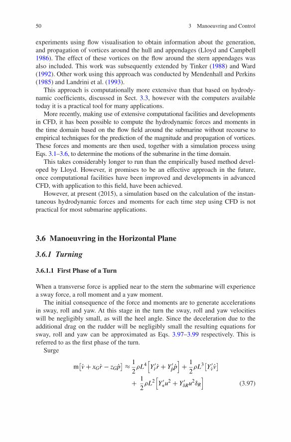
50 3 Manoeuvring and Control
experiments using flow visualisation to obtain information about the generation, and propagation of vortices around the hull and appendages (Lloyd and Campbell 1986). The effect of these vortices on the flow around the stern appendages was also included. This work was subsequently extended by Tinker (1988) and Ward (1992). Other work using this approach was conducted by Mendenhall and Perkins (1985) and Landrini et al. (1993).
This approach is computationally more extensive than that based on hydrody-namic coefficients, discussed in Sect. 3.3, however with the computers available today it is a practical tool for many applications.
More recently, making use of extensive computational facilities and developments in CFD, it has been possible to compute the hydrodynamic forces and moments in the time domain based on the flow field around the submarine without recourse to empirical techniques for the prediction of the magnitude and propagation of vortices. These forces and moments are then used, together with a simulation process using Eqs. 3.1–3.6, to determine the motions of the submarine in the time domain.
This takes considerably longer to run than the empirically based method devel-oped by Lloyd. However, it promises to be an effective approach in the future, once computational facilities have been improved and developments in advanced CFD, with application to this field, have been achieved.
However, at present (2015), a simulation based on the calculation of the instan-taneous hydrodynamic forces and moments for each time step using CFD is not practical for most submarine applications.
3.6 Manoeuvring in the Horizontal Plane
3.6.1 Turning
3.6.1.1 First Phase of a Turn
When a transverse force is applied near to the stern the submarine will experience a sway force, a roll moment and a yaw moment.
The initial consequence of the force and moments are to generate accelerations in sway, roll and yaw. At this stage in the turn the sway, roll and yaw velocities will be negligibly small, as will the heel angle. Since the deceleration due to the additional drag on the rudder will be negligibly small the resulting equations for sway, roll and yaw can be approximated as Eqs. 3.97–3.99 respectively. This is referred to as the first phase of the turn.
Surge
(3.97)
m[
v+ xGr − zGp]
≈1
2ρL4
[
Y ′r r + Y ′
pp]
+1
2ρL3
[
Y ′v v]
+1
2ρL2
[
Y ′∗u
2 + Y ′δRu
2δR
]
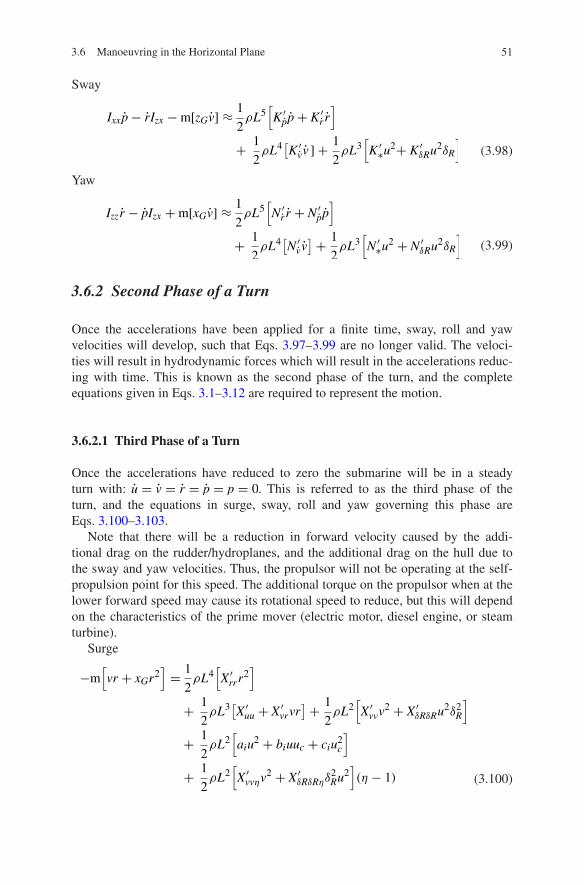
51
Sway
Yaw
3.6.2 Second Phase of a Turn
Once the accelerations have been applied for a finite time, sway, roll and yaw velocities will develop, such that Eqs. 3.97–3.99 are no longer valid. The veloci-ties will result in hydrodynamic forces which will result in the accelerations reduc-ing with time. This is known as the second phase of the turn, and the complete equations given in Eqs. 3.1–3.12 are required to represent the motion.
3.6.2.1 Third Phase of a Turn
Once the accelerations have reduced to zero the submarine will be in a steady turn with: u = v = r = p = p = 0. This is referred to as the third phase of the turn, and the equations in surge, sway, roll and yaw governing this phase are Eqs. 3.100–3.103.
Note that there will be a reduction in forward velocity caused by the addi-tional drag on the rudder/hydroplanes, and the additional drag on the hull due to the sway and yaw velocities. Thus, the propulsor will not be operating at the self-propulsion point for this speed. The additional torque on the propulsor when at the lower forward speed may cause its rotational speed to reduce, but this will depend on the characteristics of the prime mover (electric motor, diesel engine, or steam turbine).
Surge
(3.98)
Ixxp− rIzx −m[zGv] ≈1
2ρL5
[
K ′pp+ K ′
r r]
+1
2ρL4
[
K ′v v ] +
1
2ρL3
[
K ′∗u
2+ K ′δRu
2δR
]
(3.99)
Izzr − pIzx +m[xGv] ≈1
2ρL5
[
N ′r r + N ′
pp]
+1
2ρL4
[
N ′v v]
+1
2ρL3
[
N ′∗u
2 + N ′δRu
2δR
]
(3.100)
−m[
vr + xGr2]
=1
2ρL4
[
X ′rrr
2]
+1
2ρL3
[
X ′uu + X ′
vrvr]
+1
2ρL2
[
X ′vvv
2 + X ′δRδRu
2δ2R
]
+1
2ρL2
[
aiu2 + biuuc + ciu
2c
]
+1
2ρL2
[
X ′vvηv
2 + X ′δRδRηδ
2Ru
2]
(η − 1)
3.6 Manoeuvring in the Horizontal Plane
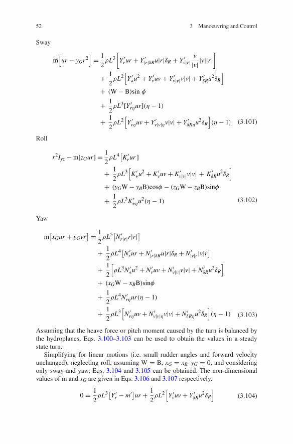
52 3 Manoeuvring and Control
Sway
Roll
Yaw
Assuming that the heave force or pitch moment caused by the turn is balanced by the hydroplanes, Eqs. 3.100–3.103 can be used to obtain the values in a steady state turn.
Simplifying for linear motions (i.e. small rudder angles and forward velocity unchanged), neglecting roll, assuming W = B, xG = xB, yG = 0, and considering only sway and yaw, Eqs. 3.104 and 3.105 can be obtained. The non-dimensional values of m and xG are given in Eqs. 3.106 and 3.107 respectively.
(3.101)
m[
ur − yGr2]
=1
2ρL3
[
Y ′rur + Y ′
|r|δRu|r|δR + Y ′v|r|
v
|v||v||r|
]
+1
2ρL2
[
Y ′∗u
2 + Y ′vuv+ Y ′
v|v|v|v| + Y ′δRu
2δR
]
+ (W− B)sin φ
+1
2ρL3[Y ′
rηur](η − 1)
+1
2ρL2
[
Y ′vηuv + Y ′
v|v|ηv|v| + Y ′δRηu
2δR
]
(η − 1)
(3.102)
r2Iyz −m[zGur] =1
2ρL4
[
K ′rur ]
+1
2ρL3
[
K ′∗u
2 + K ′vuv + K ′
v|v|v|v| + K ′δRu
2δR
]
+ (yGW− yBB)cosφ − (zGW− zBB)sinφ
+1
2ρL3K ′
∗ηu2(η − 1)
(3.103)
m[
xGur + yGvr]
=1
2ρL5
[
N ′r|r|r|r|
]
+1
2ρL4
[
N ′rur + N ′
|r|δRu|r|δR + N ′|v|r |v|r
]
+1
2
[
ρL3N ′∗u
2 + N ′vuv + N ′
v|v|v|v| + N ′δRu
2δR
]
+ (xGW− xBB)sinφ
+1
2ρL4N ′
rηur(η − 1)
+1
2ρL3
[
N ′vηuv+ N ′
v|v|ηv|v| + N ′δRηu
2δR
]
(η − 1)
(3.104)0 =1
2ρL3
[
Y ′r − m′]ur +
1
2ρL2
[
Y ′vuv + Y ′
δRu2δR
]

53
Solving the simultaneous Eqs. 3.104 and 3.105 gives Eq. 3.108 which is an expression for the turning radius, R, where R = V/r.
Equation 3.108 only applies to turns with small rudder angles, and where the cou-pling between the horizontal motions (sway and yaw) and the vertical motions (heave and pitch) can be neglected.
3.6.3 Stability in the Horizontal Plane
The stability index in the horizontal plane, GH, is given by Eq. 3.109 (Spencer 1968).
As a high degree of manoeuvrability in the horizontal plane is desirable, GH is usually a small positive value. See Sect. 3.9 for recommended values of GH.
3.6.4 Pivot Point
When turning in the horizontal plane a submarine will experience both sway and yaw. The resultant local transverse flow vectors when in a steady state turn are shown schematically in Fig. 3.16, which shows a submarine turning to port. As can be seen from this figure, the local sway velocity when turning to port is from the port side near the bow, and from the starboard side at the stern. There is one position along the length of the submarine where the local sway velocity is zero. This is referred to as the Pivot Point.
The magnitude of the local sway velocity at the stern is large. This will influ-ence the performance of the stern appendages and the propulsor when the subma-rine is undergoing a turn.
(3.105)0 =1
2ρL4
[
N ′r − m′x′G
]
ur +1
2ρL3
[
N ′vuv + N ′
δRu2δR
]
(3.106)m′ =m
12ρL3
(3.107)x′G =xG
L
(3.108)R
L=
1
δR
[
N ′v
(
Y ′r − m′)− (N ′
r − m′x′G)Y′v
N ′δY
′v − N ′
vY′δ
]
(3.109)GH = 1+N ′v(m
′ − Y ′r)
N ′rY
′v
3.6 Manoeuvring in the Horizontal Plane
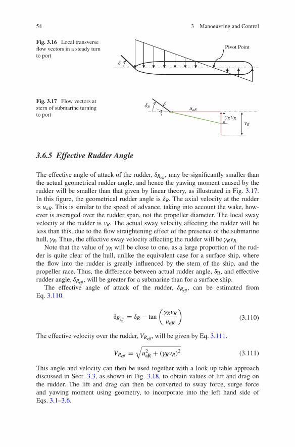
54 3 Manoeuvring and Control
3.6.5 Effective Rudder Angle
The effective angle of attack of the rudder, δReff , may be significantly smaller than the actual geometrical rudder angle, and hence the yawing moment caused by the rudder will be smaller than that given by linear theory, as illustrated in Fig. 3.17. In this figure, the geometrical rudder angle is δR. The axial velocity at the rudder is uaR. This is similar to the speed of advance, taking into account the wake, how-ever is averaged over the rudder span, not the propeller diameter. The local sway velocity at the rudder is vR. The actual sway velocity affecting the rudder will be less than this, due to the flow straightening effect of the presence of the submarine hull, γR. Thus, the effective sway velocity affecting the rudder will be γRvR.
Note that the value of γR will be close to one, as a large proportion of the rud-der is quite clear of the hull, unlike the equivalent case for a surface ship, where the flow into the rudder is greatly influenced by the stern of the ship, and the propeller race. Thus, the difference between actual rudder angle, δR, and effective rudder angle, δReff , will be greater for a submarine than for a surface ship.
The effective angle of attack of the rudder, δReff , can be estimated from Eq. 3.110.
The effective velocity over the rudder, VReff , will be given by Eq. 3.111.
This angle and velocity can then be used together with a look up table approach discussed in Sect. 3.3, as shown in Fig. 3.18, to obtain values of lift and drag on the rudder. The lift and drag can then be converted to sway force, surge force and yawing moment using geometry, to incorporate into the left hand side of Eqs. 3.1–3.6.
(3.110)δReff = δR − tan
(
γRvR
uaR
)
(3.111)VReff =√
u2aR + (γRvR)2
Fig. 3.17 Flow vectors at stern of submarine turning to port
R uaR
vR
R vR
Fig. 3.16 Local transverse flow vectors in a steady turn to port
Pivot Point

55
Note that the same principle can also apply to an X form stern. In addition, a similar approach can be used to obtain the hydrodynamic forces and moments due to the forward and aft hydroplanes when the submarine is manoeuvring in the ver-tical plane.
3.6.6 Heel in a Turn
When turning, a submarine will experience side forces on the hull and sail due to the local sway velocity. Initially this will be into the turn along the whole length of the submarine, as illustrated in Fig. 3.19.
This will result in a rolling moment, as illustrated in Fig. 3.20.As can be seen from Fig. 3.20 the force on the sail acts much higher up than the
forces on the rudder and the hull, resulting in a rolling moment into the turn. This is referred to as a ‘snap roll’ and can be a significant roll angle.
Once the submarine is in a turn the side forces on the hull and sail will depend on the local sway velocity. As the magnitude of the local sway velocity varies along the length of the submarine (Fig. 3.16) the magnitude of the sway force on the sail will depend very much on the sail’s location. If the sail is located close to the Pivot Point then the force on it will be relatively small, whereas if it is located well aft of the Pivot Point then the force may be quite large.
The other factor which will influence the magnitude of the heel in the turn is the side force generated by the sail when at an angle of attack. A large foil type sail (see Sect. 6.2) will produce a greater side force than a smaller, blended sail.
Fig. 3.18 Lift and drag on rudder as functions of δReff
3.6 Manoeuvring in the Horizontal Plane
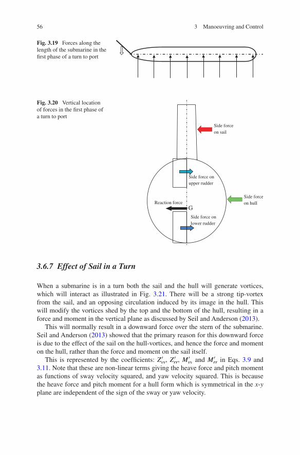
56 3 Manoeuvring and Control
3.6.7 Effect of Sail in a Turn
When a submarine is in a turn both the sail and the hull will generate vortices, which will interact as illustrated in Fig. 3.21. There will be a strong tip-vortex from the sail, and an opposing circulation induced by its image in the hull. This will modify the vortices shed by the top and the bottom of the hull, resulting in a force and moment in the vertical plane as discussed by Seil and Anderson (2013).
This will normally result in a downward force over the stern of the submarine. Seil and Anderson (2013) showed that the primary reason for this downward force is due to the effect of the sail on the hull-vortices, and hence the force and moment on the hull, rather than the force and moment on the sail itself.
This is represented by the coefficients: Z ′vv, Z
′rr, M
′vv and M ′
rr in Eqs. 3.9 and 3.11. Note that these are non-linear terms giving the heave force and pitch moment as functions of sway velocity squared, and yaw velocity squared. This is because the heave force and pitch moment for a hull form which is symmetrical in the x-y plane are independent of the sign of the sway or yaw velocity.
Fig. 3.19 Forces along the length of the submarine in the first phase of a turn to port
Fig. 3.20 Vertical location of forces in the first phase of a turn to port
G
Side forceon hull
Side force on upper rudder
Side force on lower rudder
Side force on sail
Reaction force

57
The effect of the presence of the sail on the pressure over a manoeuvring submarine hull can be seen in Fig. 3.22 from CFD data provided by the AMC. Figure 3.22a, and b show the pressure at the top and bottom of the submarine when it has zero drift angle, without and with a sail, respectively. As can be seen, when there is no sail the pressure on the top and the bottom of the hull are equal. This will result in no net force in the vertical plane, and hence the values of the coefficients: Z ′
∗ and M ′∗ will both be equal to zero.
The presence of the sail (Fig. 3.22b) results in a change in pressure at the loca-tion of the sail, however over the majority of the hull the pressures are similar. The difference due to the sail will result in a steady state heave force and pitch moment when the boat is travelling at v = r = 0. This is reflected in the values of the coef-ficients: Z ′
∗ and M ′∗ which will be non-zero for a submarine with a sail.
Figure 3.22c, and d show the pressure at the top and bottom of the submarine when it has a drift angle of 16°, without and with a sail, respectively. As expected, the pressure is reduced when the boat is at an angle to the flow. This is due to the increased velocity over the top and the bottom of the boat caused by the transverse component of the flow around the hull when it is at a drift angle.
For the case of the hull without the sail the difference in pressure between that over the top and that over the bottom is still zero, indicating that the sway veloc-ity will not cause either a heave force or a pitch moment. Hence, the values of the coefficients: Z ′
vv, Z′rr, M
′vv and M ′
rr will all be zero.However, for the case of the hull with the sail (Fig. 3.22d), the difference in
pressure over the top and bottom of the hull aft of the sail is quite marked. This will result in a non-zero values of the coefficients: Z ′
vv, Z′rr, M
′vv and M ′
rr. As the negative pressure over the top of the hull aft of the sail is less than the negative pressure over the bottom of the hull this will result in a downward force and a trimming moment bow up, thus in this case each of these coefficients will be positive.
Fig. 3.21 Vortices shed from a manoeuvring submarine (courtesy of the Australian Maritime College)
3.6 Manoeuvring in the Horizontal Plane

58 3 Manoeuvring and Control
Fig. 3.22 Pressure over the length of a manoeuvring submarine (courtesy of the Australian Maritime College). bow is at x = 0, stern is at x = 1. a Pressure at zero angle of incidence (no sail). b Pressure at zero angle of incidence (with sail). c Pressure at 16 degrees angle of incidence (no sail). d Pressure at 16 degrees angle of incidence (with sail)
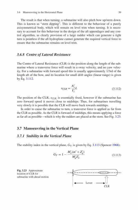
59
The result is that when turning, a submarine will also pitch bow up/stern down. This is known as “stern dipping”. This is different to the behaviour of a purely axisymmetrical body, which will remain on level trim when turning. It is neces-sary to account for this behaviour in the design of the aft appendages and any con-trol algorithm, as clearly provision of a large rudder which can generate a tight turn is pointless if the aft hydroplane cannot generate the required vertical force to ensure that the submarine remains on level trim.
3.6.8 Centre of Lateral Resistance
The Centre of Lateral Resistance (CLR) is the position along the length of the sub-marine where a transverse force will result in a sway velocity, and no yaw veloc-ity. For a submarine with forward speed this is usually approximately 1/3rd of the length aft of the bow, and its location for small drift angles (linear range) is given by Eq. 3.112.
The position of the CLR, xCLR, is essentially fixed, however if the submarine has zero forward speed it moves close to midships. Thus, for submarines travelling very slowly it is possible that the CLR will move back towards midships.
In order to cause the submarine to turn, a transverse force is applied as far from the CLR as possible. As the CLR is forward of midships, this means applying a force as far aft as possible—which is why the rudders are placed at the stern. See Fig. 3.23.
3.7 Manoeuvring in the Vertical Plane
3.7.1 Stability in the Vertical Plane
The stability index in the vertical plane, GV, is given by Eq. 3.113 (Spencer 1968).
(3.112)xCLR =N ′v
Y ′v
L
(3.113)GV = 1−M ′
w(m′ + Z ′
q)
M ′qZ
′w
Fig. 3.23 Approximate location of CLR for submarine with ahead motion
LeverCLR
3.6 Manoeuvring in the Horizontal Plane
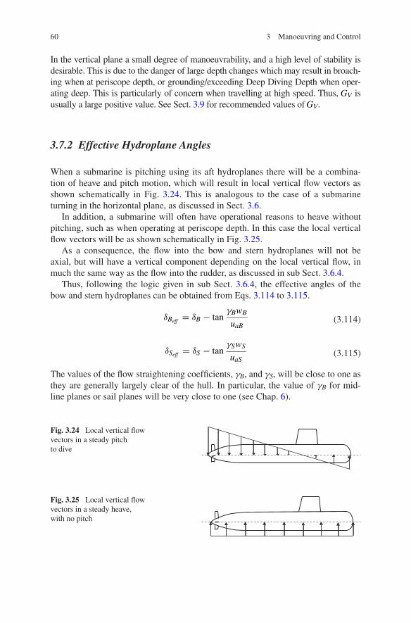
60 3 Manoeuvring and Control
In the vertical plane a small degree of manoeuvrability, and a high level of stability is desirable. This is due to the danger of large depth changes which may result in broach-ing when at periscope depth, or grounding/exceeding Deep Diving Depth when oper-ating deep. This is particularly of concern when travelling at high speed. Thus, GV is usually a large positive value. See Sect. 3.9 for recommended values of GV.
3.7.2 Effective Hydroplane Angles
When a submarine is pitching using its aft hydroplanes there will be a combina-tion of heave and pitch motion, which will result in local vertical flow vectors as shown schematically in Fig. 3.24. This is analogous to the case of a submarine turning in the horizontal plane, as discussed in Sect. 3.6.
In addition, a submarine will often have operational reasons to heave without pitching, such as when operating at periscope depth. In this case the local vertical flow vectors will be as shown schematically in Fig. 3.25.
As a consequence, the flow into the bow and stern hydroplanes will not be axial, but will have a vertical component depending on the local vertical flow, in much the same way as the flow into the rudder, as discussed in sub Sect. 3.6.4.
Thus, following the logic given in sub Sect. 3.6.4, the effective angles of the bow and stern hydroplanes can be obtained from Eqs. 3.114 to 3.115.
The values of the flow straightening coefficients, γB, and γS, will be close to one as they are generally largely clear of the hull. In particular, the value of γB for mid-line planes or sail planes will be very close to one (see Chap. 6).
(3.114)δBeff = δB − tanγBwB
uaB
(3.115)δSeff = δS − tanγSwS
uaS
Fig. 3.24 Local vertical flow vectors in a steady pitch to dive
Fig. 3.25 Local vertical flow vectors in a steady heave, with no pitch

61
The effective velocities at the bow and stern hydroplanes, VBeff , and VSeff , respectively can be obtained from Eqs. 3.116 to 3.117.
The angles and velocities can then be used together with a look up table approach discussed in Sect. 3.3, to obtain values of lift and drag on the hydroplanes, which can then be converted to heave force, surge force and pitch moment using geom-etry, to incorporate into the left hand side of Eqs. 3.1–3.6.
3.7.3 Neutral Point
The Neutral Point is the position along the length of the submarine where a verti-cal force applied will cause a change in depth, but no change in pitch angle. For submarines with high forward velocity the Neutral Point is usually approximately 1/3rd of the length aft of the bow, as shown in Fig. 3.26, and its location for small pitch angles (linear range) is given by Eq. 3.118.
When Eq. 3.112 for the location of the Centre of Lateral Resistance (CLR) is com-pared with Eq. 3.118 for the Neutral Point, it can be seen that the latter has a nega-tive sign. However, this is due to the definition of the axis system, such that for an axisymmetrical body Y ′
v = Z ′w, but N ′
v = −M ′w. Thus, for an axisymmetric body
the longitudinal position of the Centre of Lateral Resistance is the same as the longitudinal position of the Neutral Point, as expected.
When a submarine has low forward velocity, and the heave velocity is not small compared to the surge velocity, there will be a large pitch angle, (angle of attack)
(3.116)VBeff =√
u2aB + (γBwB)2
(3.117)VSeff =√
u2aS + (γSwS)2
(3.118)xNP = −M ′
w
Z ′w
L
Fig. 3.26 Approximate position of Neutral Point for submarine with high forward velocity
Neutral Point
3.7 Manoeuvring in the Vertical Plane
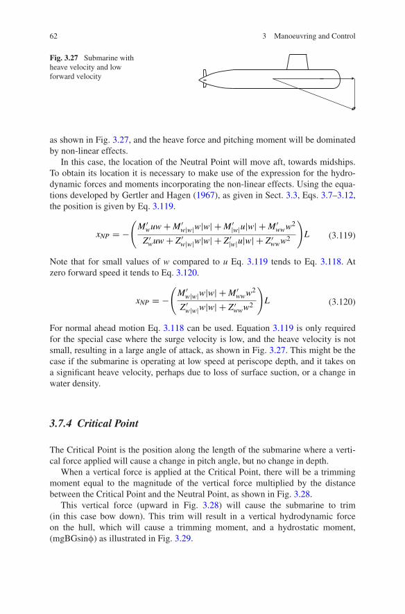
62 3 Manoeuvring and Control
as shown in Fig. 3.27, and the heave force and pitching moment will be dominated by non-linear effects.
In this case, the location of the Neutral Point will move aft, towards midships. To obtain its location it is necessary to make use of the expression for the hydro-dynamic forces and moments incorporating the non-linear effects. Using the equa-tions developed by Gertler and Hagen (1967), as given in Sect. 3.3, Eqs. 3.7–3.12, the position is given by Eq. 3.119.
Note that for small values of w compared to u Eq. 3.119 tends to Eq. 3.118. At zero forward speed it tends to Eq. 3.120.
For normal ahead motion Eq. 3.118 can be used. Equation 3.119 is only required for the special case where the surge velocity is low, and the heave velocity is not small, resulting in a large angle of attack, as shown in Fig. 3.27. This might be the case if the submarine is operating at low speed at periscope depth, and it takes on a significant heave velocity, perhaps due to loss of surface suction, or a change in water density.
3.7.4 Critical Point
The Critical Point is the position along the length of the submarine where a verti-cal force applied will cause a change in pitch angle, but no change in depth.
When a vertical force is applied at the Critical Point, there will be a trimming moment equal to the magnitude of the vertical force multiplied by the distance between the Critical Point and the Neutral Point, as shown in Fig. 3.28.
This vertical force (upward in Fig. 3.28) will cause the submarine to trim (in this case bow down). This trim will result in a vertical hydrodynamic force on the hull, which will cause a trimming moment, and a hydrostatic moment, (mgBGsinφ) as illustrated in Fig. 3.29.
(3.119)xNP = −(
M ′wuw+M ′
w|w|w|w| +M ′|w|u|w| +M ′
www2
Z ′wuw+ Z ′
w|w|w|w| + Z ′|w|u|w| + Z ′
www2
)
L
(3.120)xNP = −(
M ′w|w|w|w| +M ′
www2
Z ′w|w|w|w| + Z ′
www2
)
L
Fig. 3.27 Submarine with heave velocity and low forward velocity

63
By definition, if the vertical force is applied at the Critical Point, then it will be exactly balanced by the vertical hydrodynamic force, and the boat will not change its depth.
The hydrodynamic trimming moment will be proportional to velocity squared, whereas the hydrostatic trimming moment (mgBGsinφ) will be independent of speed.
The position of the Critical Point, xCP, is given by Eq. 3.121.
As can be seen from Eq. 3.121 the location of the Critical Point is dependent on speed. For low speeds the Critical Point can become quite far aft—even astern of the stern hydroplanes.
3.7.5 Influence of Neutral Point and Critical Point on Manoeuvring in the Vertical Plane
The influence of the Neutral Point and the Critical Point on manoeuvring in the vertical plane will depend on the speed that the submarine is travelling.(a) Submarine Travelling at Moderate Forward SpeedWhen the submarine is travelling at a moderate forward speed the position of the Neutral Point will be approximately 1/3rd of the length of the submarine aft of the bow, as discussed in sub Sect. 3.7.3. The position of the Critical Point will be slightly aft of this, as given by Eq. 3.121. This is illustrated in Fig. 3.30.
(3.121)xCP =2mgBG
ρL2Z ′wu
2− L
M ′w
Z ′w
Fig. 3.28 Upward force at Critical Point
Neutral Point
Lever
Upward force at Critical Point
Fig. 3.29 Forces on a submarine due to upward force at Critical Point
Hydrodynamic
External
BG
3.7 Manoeuvring in the Vertical Plane

64 3 Manoeuvring and Control
In this situation when an upward force is applied at the stern hydroplane the submarine will trim bow down, due to the lever between the position of applica-tion of the upward force and the location of the Neutral Point. As the upward force is applied aft of the Critical Point, the trim angle will result in a downward hydro-dynamic vertical force on the hull which is greater than the upward force at the Neutral Point, and the submarine will go downwards, as shown in Fig. 3.31.
This is the normal method of changing depth when operating at a moderate speed. The bow hydroplanes are not necessary.(b) Submarine Travelling at Low Forward SpeedAs discussed in sub Sect. 3.7.4, when the submarine is travelling at low forward speed the location of the Critical Point is much further aft, as given by Eq. 3.121. When the Critical Point coincides with the stern hydroplanes, as shown in Fig. 3.32, an upward force applied at the stern hydroplane will cause the subma-rine to trim bow down, due to the lever between the position of application of the upward force and the location of the Neutral Point, as for the moderate speed case. However, as the upward force is now applied at the Critical Point, the downward hydrodynamic vertical force on the hull, due to the trim angle, will be equal to the upward force applied by the stern hydroplanes.
This will result in the boat trimming bow down, but remaining at the same depth, since the upward force on the stern hydroplane exactly compensates for the downward hydrodynamic force on the hull, due to the trim, as shown in Fig. 3.33.
Thus, if a depth change is required when operating at low forward speeds the bow hydroplanes are required to do this. Note that if the bow hydroplanes are at the Neutral Point, then they cannot change the trim angle. They can only apply a vertical downward force to cause a decent. On the other hand, if the bow hydro-planes are forward of the Neutral Point then they can also be used to increase the
Fig. 3.31 Submarine diving when upward force at stern hydroplane is aft of Critical Point
Critical Point Neutral
Point
Upward force at stern hydroplane
Downward hydrodynamic force
on hull
Fig. 3.30 Positions of neutral point and critical point for a submarine at moderate speed
Neutral Point
Critical Point
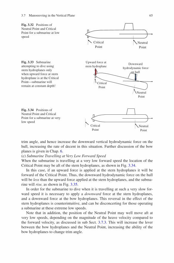
65
trim angle, and hence increase the downward vertical hydrodynamic force on the hull, increasing the rate of decent in this situation. Further discussion of the bow planes is given in Chap. 6.(c) Submarine Travelling at Very Low Forward SpeedWhen the submarine is travelling at a very low forward speed the location of the Critical Point may be aft of the stern hydroplanes, as shown in Fig. 3.34.
In this case, if an upward force is applied at the stern hydroplanes it will be forward of the Critical Point. Thus, the downward hydrodynamic force on the hull will be less than the upward force applied at the stern hydroplanes, and the subma-rine will rise, as shown in Fig. 3.35.
In order for the submarine to dive when it is travelling at such a very slow for-ward speed it is necessary to apply a downward force at the stern hydroplanes, and a downward force at the bow hydroplanes. This reversal in the effect of the stern hydroplanes is counterintuitive, and can be disconcerting for those operating a submarine at these extreme low speeds.
Note that in addition, the position of the Neutral Point may well move aft at very low speeds, depending on the magnitude of the heave velocity compared to the forward velocity, as discussed in sub Sect. 3.7.3. This will increase the lever between the bow hydroplanes and the Neutral Point, increasing the ability of the bow hydroplanes to change trim angle.
Fig. 3.32 Positions of Neutral Point and Critical Point for a submarine at low speed
Neutral Point
Critical Point
Fig. 3.33 Submarine attempting to dive using stern hydroplanes only when upward force at stern hydroplane is at the Critical Point—submarine will remain at constant depth!
Upward force at stern hydroplane
Downward hydrodynamic force
on hull
Critical Point
Neutral Point
Fig. 3.34 Positions of Neutral Point and Critical Point for a submarine at very low speed
Neutral Point
Critical Point
3.7 Manoeuvring in the Vertical Plane
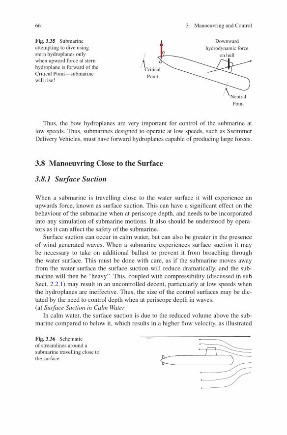
66 3 Manoeuvring and Control
Thus, the bow hydroplanes are very important for control of the submarine at low speeds. Thus, submarines designed to operate at low speeds, such as Swimmer Delivery Vehicles, must have forward hydroplanes capable of producing large forces.
3.8 Manoeuvring Close to the Surface
3.8.1 Surface Suction
When a submarine is travelling close to the water surface it will experience an upwards force, known as surface suction. This can have a significant effect on the behaviour of the submarine when at periscope depth, and needs to be incorporated into any simulation of submarine motions. It also should be understood by opera-tors as it can affect the safety of the submarine.
Surface suction can occur in calm water, but can also be greater in the presence of wind generated waves. When a submarine experiences surface suction it may be necessary to take on additional ballast to prevent it from broaching through the water surface. This must be done with care, as if the submarine moves away from the water surface the surface suction will reduce dramatically, and the sub-marine will then be “heavy”. This, coupled with compressibility (discussed in sub Sect. 2.2.1) may result in an uncontrolled decent, particularly at low speeds when the hydroplanes are ineffective. Thus, the size of the control surfaces may be dic-tated by the need to control depth when at periscope depth in waves.(a) Surface Suction in Calm Water
In calm water, the surface suction is due to the reduced volume above the sub-marine compared to below it, which results in a higher flow velocity, as illustrated
Fig. 3.36 Schematic of streamlines around a submarine travelling close to the surface
Fig. 3.35 Submarine attempting to dive using stern hydroplanes only when upward force at stern hydroplane is forward of the Critical Point—submarine will rise!
Critical Point
Neutral Point
Downward hydrodynamic force
on hull

67
in Fig. 3.36 (streamlines closer together) and hence a lower pressure. This is simi-lar to the case of a surface ship in the horizontal plane when it is travelling close to a bank, or close to the seabed, where the phenomenon is known as squat.
Surface suction can be represented in the equations of the forces and moments acting on the submarine, such as those given in Eqs. 3.9–3.12 by making Z ′
∗ a function of H∗, the non-dimensional distance from the water surface, defined in Eq. 3.122.
H is the distance from the surface to the centreline, and D is the diameter of the submarine, as shown in Fig. 3.37.
The additional complication compared to a surface ship travelling close to a boundary is that the free surface boundary is not flat. When the submarine is travelling close to the water surface, surface waves are generated, as shown in Fig. 3.38. This is discussed further in Chap. 4 in the context of the additional drag generated by a submarine close to the surface.
The wave pattern generated by the submarine complicates the surface suction effect. As these surface waves are a function of Froude number, Fr, the surface suction can be represented as given in Eq. 3.123.
(3.122)H∗ =H
D
(3.123)Surface suction = Z ′∗(H
∗,Fr)
Fig. 3.37 Definition of H and D
H
D
Fig. 3.38 Photograph of surface waves generated by a submarine model close to the surface model is towed using a sting, as shown in Fig. 3.4. H* = 1.1; Fr = 0.133. (courtesy of the Australian Maritime College)
3.8 Manoeuvring Close to the Surface
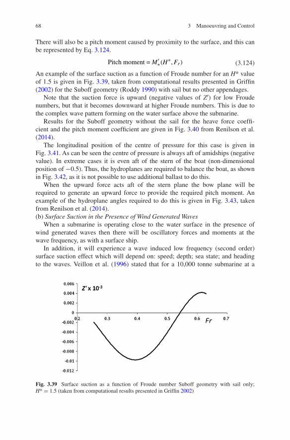
68 3 Manoeuvring and Control
There will also be a pitch moment caused by proximity to the surface, and this can be represented by Eq. 3.124.
An example of the surface suction as a function of Froude number for an H* value of 1.5 is given in Fig. 3.39, taken from computational results presented in Griffin (2002) for the Suboff geometry (Roddy 1990) with sail but no other appendages.
Note that the suction force is upward (negative values of Z′) for low Froude numbers, but that it becomes downward at higher Froude numbers. This is due to the complex wave pattern forming on the water surface above the submarine.
Results for the Suboff geometry without the sail for the heave force coeffi-cient and the pitch moment coefficient are given in Fig. 3.40 from Renilson et al. (2014).
The longitudinal position of the centre of pressure for this case is given in Fig. 3.41. As can be seen the centre of pressure is always aft of amidships (negative value). In extreme cases it is even aft of the stern of the boat (non-dimensional position of −0.5). Thus, the hydroplanes are required to balance the boat, as shown in Fig. 3.42, as it is not possible to use additional ballast to do this.
When the upward force acts aft of the stern plane the bow plane will be required to generate an upward force to provide the required pitch moment. An example of the hydroplane angles required to do this is given in Fig. 3.43, taken from Renilson et al. (2014).(b) Surface Suction in the Presence of Wind Generated Waves
When a submarine is operating close to the water surface in the presence of wind generated waves then there will be oscillatory forces and moments at the wave frequency, as with a surface ship.
In addition, it will experience a wave induced low frequency (second order) surface suction effect which will depend on: speed; depth; sea state; and heading to the waves. Veillon et al. (1996) stated that for a 10,000 tonne submarine at a
(3.124)Pitch moment = M ′∗(H
∗,Fr)
Fig. 3.39 Surface suction as a function of Froude number Suboff geometry with sail only; H* = 1.5 (taken from computational results presented in Griffin 2002)
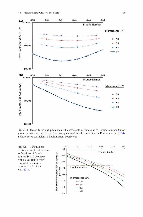
69
Fig. 3.40 Heave force and pitch moment coefficients as functions of Froude number Suboff geometry with no sail (taken from computational results presented in Renilson et al. 2014). a Heave force coefficient. b Pitch moment coefficient
Fig. 3.41 Longitudinal position of centre of pressure as functions of Froude number Suboff geometry with no sail (taken from computational results presented in Renilson et al. 2014)
3.8 Manoeuvring Close to the Surface

70 3 Manoeuvring and Control
depth of 50 m the surface suction due to waves will require around 20–30 tonnes of compensation to stop the submarine from surfacing.
Calculation of both the first order and the second order wave forces and moments can be carried out using potential flow, as discussed by Musker (1984).
The first order force and moment, at the same frequency as the waves, are functions of wave height, but the second order force and moment, are func-tions of wave height squared. Thus, they can be non-dimensionalised as given in Eqs. 3.125–3.128 (Crossland 2013).
(3.125)Z ′RAO =
ZRAO
ρgL2ζw
Fig. 3.42 Schematic of the additional forces acting on the submarine when close to the free surface
Upward suction force
Force on stern plane Force on bow plane
Fig. 3.43 Variation in plane angles required as functions of Froude number Suboff geometry with no sail (taken from computational results presented in Renilson et al. 2014). a Stern plane. b Bow plane
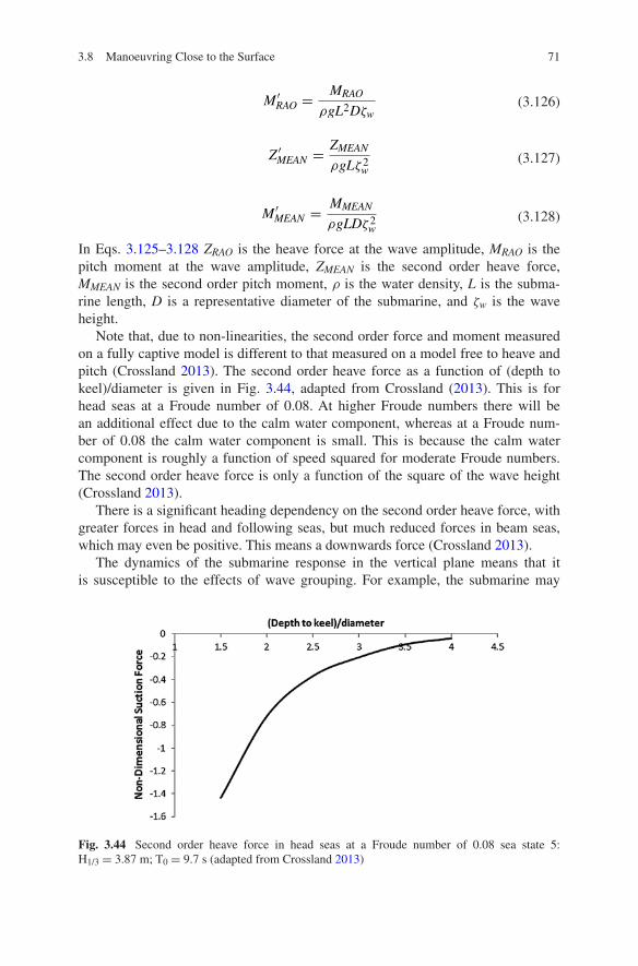
71
In Eqs. 3.125–3.128 ZRAO is the heave force at the wave amplitude, MRAO is the pitch moment at the wave amplitude, ZMEAN is the second order heave force, MMEAN is the second order pitch moment, ρ is the water density, L is the subma-rine length, D is a representative diameter of the submarine, and ζw is the wave height.
Note that, due to non-linearities, the second order force and moment measured on a fully captive model is different to that measured on a model free to heave and pitch (Crossland 2013). The second order heave force as a function of (depth to keel)/diameter is given in Fig. 3.44, adapted from Crossland (2013). This is for head seas at a Froude number of 0.08. At higher Froude numbers there will be an additional effect due to the calm water component, whereas at a Froude num-ber of 0.08 the calm water component is small. This is because the calm water component is roughly a function of speed squared for moderate Froude numbers. The second order heave force is only a function of the square of the wave height (Crossland 2013).
There is a significant heading dependency on the second order heave force, with greater forces in head and following seas, but much reduced forces in beam seas, which may even be positive. This means a downwards force (Crossland 2013).
The dynamics of the submarine response in the vertical plane means that it is susceptible to the effects of wave grouping. For example, the submarine may
(3.126)M ′RAO =
MRAO
ρgL2Dζw
(3.127)Z ′MEAN =
ZMEAN
ρgLζ 2w
(3.128)M ′MEAN =
MMEAN
ρgLDζ 2w
Fig. 3.44 Second order heave force in head seas at a Froude number of 0.08 sea state 5: H1/3 = 3.87 m; T0 = 9.7 s (adapted from Crossland 2013)
3.8 Manoeuvring Close to the Surface

72 3 Manoeuvring and Control
encounter groups of large waves for a period of time, resulting in an increase in surface suction. This must be opposed by a combination of the control surfaces and the ballast system to avoid the submarine broaching through the water surface. This means that the size of the control surfaces and the design of the ballast sys-tem need to be considered together, and the design may be determined by the need to control depth when at periscope depth in waves.
3.8.2 Manoeuvring in the Vertical Plane
When a submarine is deeply submerged the forces and moments on it are dependent only on the motions (velocities and accelerations), propeller rpm, and appendage angles as discussed in Sect. 3.3. This was used to develop Eqs. 3.7–3.13. Thus, the hydrodynamic forces and moments are independent of the depth of the submarine, and the trim angle.
However, when a submarine is operating close to the surface the hydrodynamic forces and moments on it will be functions of the depth of the submarine, H, and the trim angle, τ, as defined in Fig. 3.45.
Note that the trim angle is not the same as the pitch angle, θ, since it is meas-ured relative to the water surface, not the direction that the submarine is travelling. However, in the special case where the submarine is moving parallel to the water surface, these are the same.
Thus, additional terms are required in Eqs. 3.9 and 3.11 to represent the effect of the presence of the water surface on the hydrodynamic forces and moments, as given in Table 3.7.
In addition, in principle when a submarine is operating close to the surface all the hydrodynamic coefficients in Eqs. 3.9 and 3.11, (which are for the vertical force, Z, and the pitch moment, M, respectively) should be functions of H*, τ, and Fr. In practice it is not necessary to consider all of them as functions of H*, τ, and Fr, as the effect of the relatively minor changes in some of these coefficients as the vessel is closer to the surface are negligible (Broglia et al. 2007; Polis et al. 2013).
Conducting captive experiments to investigate the hydrodynamic forces and moments when operating in the vertical plane close to the surface has to be done with great care. Unlike the deep water situation, where the model can be tested
Fig. 3.45 Definition of trim angle, τ
τ
H
O
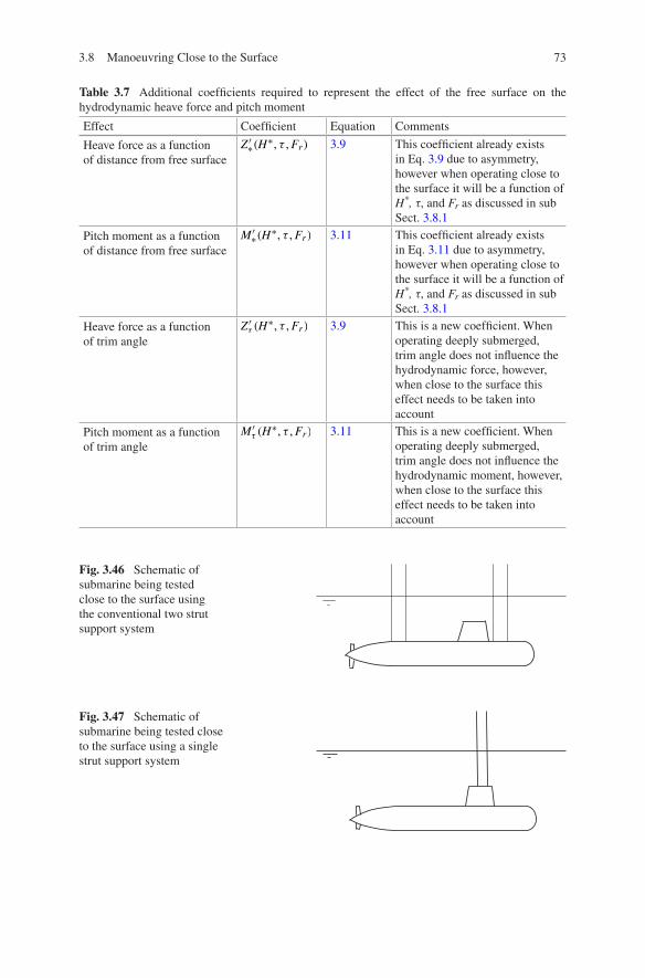
73
Table 3.7 Additional coefficients required to represent the effect of the free surface on the hydrodynamic heave force and pitch moment
Effect Coefficient Equation Comments
Heave force as a function of distance from free surface
Z ′∗(H
∗, τ ,Fr) 3.9 This coefficient already exists in Eq. 3.9 due to asymmetry, however when operating close to the surface it will be a function of H*, τ, and Fr as discussed in sub Sect. 3.8.1
Pitch moment as a function of distance from free surface
M ′∗(H
∗, τ ,Fr) 3.11 This coefficient already exists in Eq. 3.11 due to asymmetry, however when operating close to the surface it will be a function of H*, τ, and Fr as discussed in sub Sect. 3.8.1
Heave force as a function of trim angle
Z ′τ (H
∗, τ ,Fr) 3.9 This is a new coefficient. When operating deeply submerged, trim angle does not influence the hydrodynamic force, however, when close to the surface this effect needs to be taken into account
Pitch moment as a function of trim angle
M ′τ (H
∗, τ ,Fr) 3.11 This is a new coefficient. When operating deeply submerged, trim angle does not influence the hydrodynamic moment, however, when close to the surface this effect needs to be taken into account
Fig. 3.46 Schematic of submarine being tested close to the surface using the conventional two strut support system
Fig. 3.47 Schematic of submarine being tested close to the surface using a single strut support system
3.8 Manoeuvring Close to the Surface
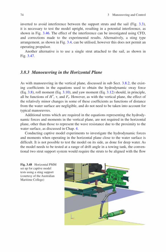
74 3 Manoeuvring and Control
inverted to avoid interference between the support struts and the sail (Fig. 3.3), it is necessary to test the model upright, resulting in a potential interference, as shown in Fig. 3.46. The effect of the interference can be investigated using CFD, and corrections made to the experimental results. Alternatively, a sting type arrangement, as shown in Fig. 3.4, can be utilised, however this does not permit an operating propulsor.
Another alternative is to use a single strut attached to the sail, as shown in Fig. 3.47.
3.8.3 Manoeuvring in the Horizontal Plane
As with manoeuvring in the vertical plane, discussed in sub Sect. 3.8.2, the exist-ing coefficients in the equations used to obtain the hydrodynamic sway force (Eq. 3.8), roll moment (Eq. 3.10), and yaw moment (Eq. 3.12) should, in principle, all be functions of H*, τ, and Fr. However, as with the vertical plane, the effect of the relatively minor changes in some of these coefficients as functions of distance from the water surface are negligible, and do not need to be taken into account for typical manoeuvres.
Additional terms which are required in the equations representing the hydrody-namic forces and moments in the vertical plane, are not required in the horizontal plane, other than those to represent the wave resistance due to the proximity to the water surface, as discussed in Chap. 4.
Conducting captive model experiments to investigate the hydrodynamic forces and moments when operating in the horizontal plane close to the water surface is difficult. It is not possible to test the model on its side, as done for deep water. As the model needs to be tested at a range of drift angle in a towing tank, the conven-tional two strut support system would require the struts to be aligned with the flow
Fig. 3.48 Horizontal PMM set up for captive model tests using a sting support (courtesy of the Australian Maritime College)

75
for each drift angle. Equally, care needs to be taken when testing close to the sur-face using a rotating arm to avoid interaction with the support struts.
An alternative is to use a Horizontal PMM (HPMM) with the model attached using a sting, as shown in Fig. 3.48. Here, the model origin is located directly below the PMM support strut, and the sting curved to attach to the model at its stern. With this mechanism it is not possible to have a rotating propulsor, however it may be adequate to investigate the influence of the water surface on the coeffi-cients representing the hydrodynamic force and moments on the submarine in the horizontal plane.
3.9 Manoeuvring Criteria
A recommended range for the various manoeuvring criteria is given in Table 3.8, taken from Ray et al. (2008). This is adequate at the initial design stage to determine the required size of both fixed and control appendages.
3.10 Manoeuvring Limitation Diagrams
3.10.1 Introduction
Manoeuvring limitations are placed on a submarine to ensure that it is operated in such a way that it can survive a “credible failure”. These limitations are depicted using Manoeuvring Limitation Diagrams (MLDs) which are then used by the crew to ensure that the submarine does not get into a situation from which it cannot recover. In the past MLDs have been displayed graphically on paper, however it is also possible for them to be displayed using the on-board electronic display consoles.
Table 3.8 Recommended range of stability and control indices (taken from Ray et al. 2008)
Parameter Expression Acceptable range
Vertical stability index GV 0.5–0.8
Horizontal stability index GH 0.2–0.4
Stern planes heave effectiveness Z ′δS/
[
(0.001L)(
Z ′w − m′)] 2.5–4.5
Stern planes pitch effectiveness M ′δS/
[
(
0.001L2)
(
M ′q − I ′yy
)]
0.2–0.4
Bow planes heave effectiveness Z ′δB/
[
(0.001L)(
Z ′w − m′)] 0.7–1.7
Bow planes pitch effectiveness M ′δB/
[
(
0.001L2)
(
M ′q − I ′yy
)]
−0.8 to −0.2
Rudder sway effectiveness Y ′δR/
[
(0.001L)(
m′ − Y ′v
)]
3.0–5.0
Rudder yaw effectiveness N ′δR/
[(
0.001L2)(
N ′r − I ′zz
)]
0.2–0.6
3.8 Manoeuvring Close to the Surface

76 3 Manoeuvring and Control
Typical “credible failures” include the following:
(a) permanent plane jams, usually at the last ordered angle;(b) temporary plane jams at the maximum angle;(c) runaway plane, where the plane moves to the hard over position due to a
failure of the control system;(d) securable and unsecurable floods; and(e) failure of power.
As part of the submarine safety assessment, these, and any other “credible failures”, must be determined, and the probability of occurrence obtained.
To generate a MLD it is necessary to have a manoeuvring simulation model of the submarine. As this is a “safety critical” element, such software must be cor-rectly verified and validated. It is also necessary to know the Standard Operating Procedures (SOPs) which the crew will conduct in the event of each failure, including an estimate of the crew reaction time.
MLDs are then generated by running the simulations for a wide range of condi-tions, including at least two initial conditions, and assessing the trajectory of the submarine to determine whether or not it will survive. For this reason a validated simulation model is required which can be run reasonably quickly, as there are numerous conditions to assess.
A factor of safety must be applied to the results to account for unknown factors, such as: inaccuracy of the manoeuvring simulation model; crew reaction time; and initial conditions.
A typical MLD for a submarine with a cruciform stern is shown schematically in Fig. 3.49.
3.10.2 Aft Hydroplane Jam
A typical SOP for an aft hydroplane jam on a submarine with a cruciform stern is as follows:
Fig. 3.49 Typical MLD for a submarine with a cruciform stern
Speed
Risk of broaching
No Restriction on Restrictionhydroplane angles on hydroplane
anglesFlood avoid zone
Depth
DDDRisk of depth excursion
MED

77
(a) order full astern rpm;(b) operate bow hydroplanes if they are available; and(c) hold the rudder amidships.
Thus, to be able to simulate the resulting motions of the submarine after a stern hydroplane jam it is necessary to understand the behaviour of the prime mover (how long it will take to generate power astern, and the relationship between power and rpm), and the hydrodynamic forces on the propulsor when going astern.
Failure after a stern plane jam will occur if the submarine:
(a) exceeds Maximum Excursion Depth (MED);(b) hits the seabed;(c) reaches the surface proximity limit; or(d) develops an excessive trim angle.
Success after a plane jam incident is defined as:
(a) MED/seabed or proximity to the water surface not exceeded;(b) maximum permissible trim angle is not exceeded;(c) a trajectory in the opposite direction to the jam is achieved; and(d) Post recovery speed is maintained.
3.10.3 Flooding
Flooding can occur through systems connected to the sea which are normally kept closed.
A typical SOP for a flooding incident is as follows:
(a) secure the submarine, if possible;(b) apply full forward rpm, if available;(c) blow all main ballast tanks; and(d) drive the submarine to the surface.
For diesel electric submarines flooding may result in the loss of power if the flood occurs in a compartment containing propulsion equipment, including batteries. This needs to be taken into account in the simulation.
Success after a flooding incident is defined as:
(a) MED or seabed not exceeded;(b) maximum permissible trim angle is not exceeded; and(c) submarine must reach the surface with an acceptable level of reserve
buoyancy.
High rates of rise, and unpowered ascents where the submarine may ascend stern first, are difficult to model, and great care needs to be taken when a simulation
3.10 Manoeuvring Limitation Diagrams
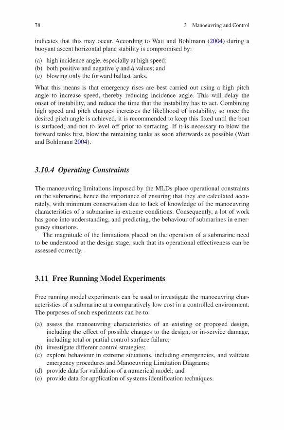
78 3 Manoeuvring and Control
indicates that this may occur. According to Watt and Bohlmann (2004) during a buoyant ascent horizontal plane stability is compromised by:
(a) high incidence angle, especially at high speed;(b) both positive and negative q and q values; and(c) blowing only the forward ballast tanks.
What this means is that emergency rises are best carried out using a high pitch angle to increase speed, thereby reducing incidence angle. This will delay the onset of instability, and reduce the time that the instability has to act. Combining high speed and pitch changes increases the likelihood of instability, so once the desired pitch angle is achieved, it is recommended to keep this fixed until the boat is surfaced, and not to level off prior to surfacing. If it is necessary to blow the forward tanks first, blow the remaining tanks as soon afterwards as possible (Watt and Bohlmann 2004).
3.10.4 Operating Constraints
The manoeuvring limitations imposed by the MLDs place operational constraints on the submarine, hence the importance of ensuring that they are calculated accu-rately, with minimum conservatism due to lack of knowledge of the manoeuvring characteristics of a submarine in extreme conditions. Consequently, a lot of work has gone into understanding, and predicting, the behaviour of submarines in emer-gency situations.
The magnitude of the limitations placed on the operation of a submarine need to be understood at the design stage, such that its operational effectiveness can be assessed correctly.
3.11 Free Running Model Experiments
Free running model experiments can be used to investigate the manoeuvring char-acteristics of a submarine at a comparatively low cost in a controlled environment. The purposes of such experiments can be to:
(a) assess the manoeuvring characteristics of an existing or proposed design, including the effect of possible changes to the design, or in-service damage, including total or partial control surface failure;
(b) investigate different control strategies;(c) explore behaviour in extreme situations, including emergencies, and validate
emergency procedures and Manoeuvring Limitation Diagrams;(d) provide data for validation of a numerical model; and(e) provide data for application of systems identification techniques.
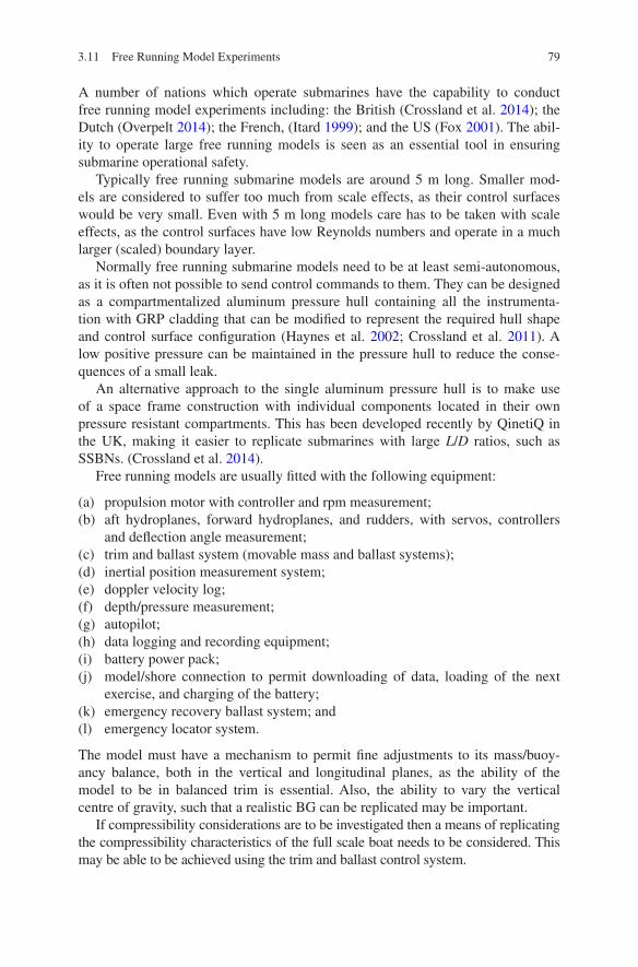
79
A number of nations which operate submarines have the capability to conduct free running model experiments including: the British (Crossland et al. 2014); the Dutch (Overpelt 2014); the French, (Itard 1999); and the US (Fox 2001). The abil-ity to operate large free running models is seen as an essential tool in ensuring submarine operational safety.
Typically free running submarine models are around 5 m long. Smaller mod-els are considered to suffer too much from scale effects, as their control surfaces would be very small. Even with 5 m long models care has to be taken with scale effects, as the control surfaces have low Reynolds numbers and operate in a much larger (scaled) boundary layer.
Normally free running submarine models need to be at least semi-autonomous, as it is often not possible to send control commands to them. They can be designed as a compartmentalized aluminum pressure hull containing all the instrumenta-tion with GRP cladding that can be modified to represent the required hull shape and control surface configuration (Haynes et al. 2002; Crossland et al. 2011). A low positive pressure can be maintained in the pressure hull to reduce the conse-quences of a small leak.
An alternative approach to the single aluminum pressure hull is to make use of a space frame construction with individual components located in their own pressure resistant compartments. This has been developed recently by QinetiQ in the UK, making it easier to replicate submarines with large L/D ratios, such as SSBNs. (Crossland et al. 2014).
Free running models are usually fitted with the following equipment:
(a) propulsion motor with controller and rpm measurement;(b) aft hydroplanes, forward hydroplanes, and rudders, with servos, controllers
and deflection angle measurement;(c) trim and ballast system (movable mass and ballast systems);(d) inertial position measurement system;(e) doppler velocity log;(f) depth/pressure measurement;(g) autopilot;(h) data logging and recording equipment;(i) battery power pack;(j) model/shore connection to permit downloading of data, loading of the next
exercise, and charging of the battery;(k) emergency recovery ballast system; and(l) emergency locator system.
The model must have a mechanism to permit fine adjustments to its mass/buoy-ancy balance, both in the vertical and longitudinal planes, as the ability of the model to be in balanced trim is essential. Also, the ability to vary the vertical centre of gravity, such that a realistic BG can be replicated may be important.
If compressibility considerations are to be investigated then a means of replicating the compressibility characteristics of the full scale boat needs to be considered. This may be able to be achieved using the trim and ballast control system.
3.11 Free Running Model Experiments
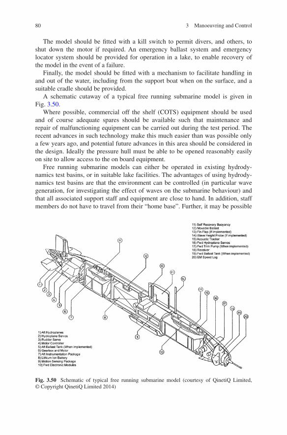
80 3 Manoeuvring and Control
The model should be fitted with a kill switch to permit divers, and others, to shut down the motor if required. An emergency ballast system and emergency locator system should be provided for operation in a lake, to enable recovery of the model in the event of a failure.
Finally, the model should be fitted with a mechanism to facilitate handling in and out of the water, including from the support boat when on the surface, and a suitable cradle should be provided.
A schematic cutaway of a typical free running submarine model is given in Fig. 3.50.
Where possible, commercial off the shelf (COTS) equipment should be used and of course adequate spares should be available such that maintenance and repair of malfunctioning equipment can be carried out during the test period. The recent advances in such technology make this much easier than was possible only a few years ago, and potential future advances in this area should be considered in the design. Ideally the pressure hull must be able to be opened reasonably easily on site to allow access to the on board equipment.
Free running submarine models can either be operated in existing hydrody-namics test basins, or in suitable lake facilities. The advantages of using hydrody-namics test basins are that the environment can be controlled (in particular wave generation, for investigating the effect of waves on the submarine behaviour) and that all associated support staff and equipment are close to hand. In addition, staff members do not have to travel from their “home base”. Further, it may be possible
Fig. 3.50 Schematic of typical free running submarine model (courtesy of QinetiQ Limited, © Copyright QinetiQ Limited 2014)

81
to set up an ability to communicate with the model, and it is generally visible dur-ing the tests.
On the other hand, few hydrodynamics test basins are deep enough to permit depth changing manoeuvres, and hence any serious free running model capability must have access to a suitable lake test facility.
The requirements of a lake test facility include the following:
(a) sufficient area to permit a range of manoeuvres without encroaching on the shallow areas at the edges: for a 5 m model an area of at least 200 m × 200 m of deep water is required, but greater area is desirable, in which case multiple manoeuvres can be carried out in each run;
(b) suitable depth to permit depth changing manoeuvres, but not too deep to result in the loss of the model in the event of a failure: for a 5 m model a depth of 20–30 m is ideal;
(c) ability to easily launch and recover the submarine model and the support boat;(d) suitable office and workshop accommodation, with power, for the trials crew,
and secure storage for the model and equipment;(e) facilities for calibrating measuring equipment, if necessary;(f) facilities for diver operations, if required;(g) adequate shelter, in particular from wind and wind generated waves;(h) lack of water currents;(i) temperature and density consistency; and(j) sufficient privacy, preferably with no other users, when the free running trials
are being conducted.
In addition the lake must be either sufficiently close to the “home base” to enable staff to return home each evening, or be located close to amenities such as hotel accommodation and restaurants/shops, including hardware outlets. It should also be sufficiently accessible to clients and other personnel who require brief visits during the test periods.
3.12 Submarine Manoeuvring Trials
3.12.1 Introduction
Full scale manoeuvring trials are conducted on submarines for the following different purposes:
(a) to confirm whether design specifications have been met (either on the initial design, or after modifications); and
(b) to generate data to improve future predictions of submarine manoeuvring.
The generation of data is particularly important, especially to help to understand the correlation between model and full scale manoeuvring performance.
3.11 Free Running Model Experiments
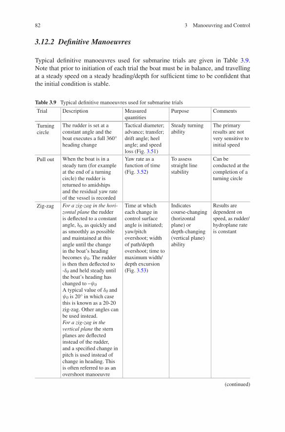
82 3 Manoeuvring and Control
3.12.2 Definitive Manoeuvres
Typical definitive manoeuvres used for submarine trials are given in Table 3.9. Note that prior to initiation of each trial the boat must be in balance, and travelling at a steady speed on a steady heading/depth for sufficient time to be confident that the initial condition is stable.
Table 3.9 Typical definitive manoeuvres used for submarine trials
Trial Description Measured quantities
Purpose Comments
Turning circle
The rudder is set at a constant angle and the boat executes a full 360° heading change
Tactical diameter; advance; transfer; drift angle; heel angle; and speed loss (Fig. 3.51)
Steady turning ability
The primary results are not very sensitive to initial speed
Pull out When the boat is in a steady turn (for example at the end of a turning circle) the rudder is returned to amidships and the residual yaw rate of the vessel is recorded
Yaw rate as a function of time (Fig. 3.52)
To assess straight line stability
Can be conducted at the completion of a turning circle
Zig-zag For a zig-zag in the hori-zontal plane the rudder is deflected to a constant angle, δ0, as quickly and as smoothly as possible and maintained at this angle until the change in the boat’s heading becomes ψ0. The rudder is then then deflected to -δ0 and held steady until the boat’s heading has changed to –ψ0A typical value of δ0 and ψ0 is 20° in which case this is known as a 20-20 zig-zag. Other angles can be used instead.For a zig-zag in the vertical plane the stern planes are deflected instead of the rudder, and a specified change in pitch is used instead of change in heading. This is often referred to as an overshoot manoeuvre
Time at which each change in control surface angle is initiated; yaw/pitch overshoot; width of path/depth overshoot; time to maximum width/depth excursion (Fig. 3.53)
Indicates course-changing (horizontal plane) or depth-changing (vertical plane) ability
Results are dependent on speed, as rudder/hydroplane rate is constant
(continued)

83
Trial Description Measured quantities
Purpose Comments
Meander This is similar to the zig-zag manoeuvre in the vertical plane, with the difference that once the execute pitch angle is reached, the control surfaces are brought to zero (and not reversed as in the zig-zag or overshoot test)
Path of vessel Indicates motion stability and depth keeping ability
Spiral The rudder is deflected to a given maximum angle, such as 25°, and held until a steady yaw rate is obtained (A in Fig. 3.54). It is then reduced by a fixed increment (such as 5°) and held until a steady yaw rate is obtained. This is repeated until the opposite value of the initial maximum angle is reached (F in Fig. 3.54) with the steady yaw rate recorded at each increment. The process is then repeated in the opposite direction until the initial maximum rudder angle is achieved (A in Fig. 3.54)
Steady yaw rate for each rudder angle (Fig. 3.54)
Control authority and straight line stability.The size of the hysteresis loop, BDEH shown in Fig. 3.54b is a measure of instability
Care needs to be taken to ensure that the yaw rate is steady at each increment.The results are not very sensitive to initial speed.This test can be very time consuming, and does not give information within the hysteresis loop for unstable boats
Reverse spiral
The rudder angle required to achieve a given yaw rate is determined. This is then repeated for a range of different yaw angles
Steady yaw rate for each rudder angle
Control author-ity and straight line stability
The results are not very sensitive to initial speed. For an unstable boat this gives infor-mation within the hysteresis loop
Table 3.9 (continued)
Typical results from these definitive manoeuvres are given in Figs. 3.51, 3.52, 3.53 and 3.54
Also, for tests in the horizontal plane it may be necessary to operate the for-ward and aft hydroplanes to ensure that the boat remains at constant trim and depth, as the asymmetry due to the casing and the sail will result in a vertical force and pitching moment when turning, as discussed in sub Sect. 3.6.6.
3.12 Submarine Manoeuvring Trials
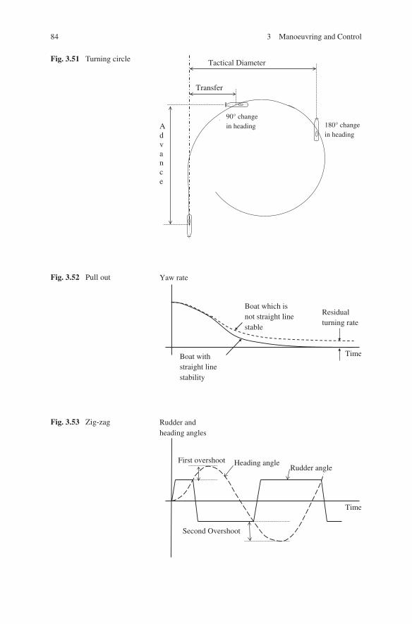
84 3 Manoeuvring and Control
Fig. 3.51 Turning circle
Advance
Tactical Diameter
Transfer
180° change in heading
90° change in heading
Fig. 3.52 Pull out
Residual turning rate
Boat which is not straight line stable
TimeBoat with straight line stability
Yaw rate
Fig. 3.53 Zig-zag
Rudder angleHeading angle
Time
Second Overshoot
First overshoot
Rudder and heading angles

85
3.12.3 Preparation for the Trials
Prior to conducting the trial it is very important to determine exactly the purpose of the trial. For example, is it purely to determine whether a new boat meets the design specification, or is it to generate new data to validate a manoeuvring code? If the former, it is clear which boat the trials need to be conducted on, whereas if the latter then the submarine selected will depend on considerations such as availability.
Once the purpose of the trial has been agreed, then trials orders need to be drawn up. These will include the following (Bayliss et al. 2005):
(a) scope and high level requirement;(b) equipment fit required;(c) trial programme;
Fig. 3.54 Spiral test. a Straight line stable. b Straight line unstable
Rudder angle
Rate of turn
A
B
H C
G D
E
F
Rudder angle
Rate of turnA
B
C
D
E
F
G
H
(a)
(b)
3.12 Submarine Manoeuvring Trials

86 3 Manoeuvring and Control
(d) trials team and civilian personnel;(e) detailed list of runs, including all requirements for each run; and(f) risk assessment/safety case.
Determination and proper specification of the trials equipment is essential, includ-ing the required accuracy of any measuring instrumentation. It may be possible to make use of the existing submarine platform management system to measure, and record, some of the required data (Tickle et al. 2014). Whether this is possible, or not, and the effect that it could have on operations, needs to be understood at an early stage.
Also, any devices which affect the movement of the control surfaces need to be agreed upon well in advance, and taken into account in the risk assessment/safety case for the trial.
When planning the trials, and even when selecting which boat to use, consider-ation needs to be given to the boat’s operational program in the months prior to the trial. Specialist equipment may be required, and this will require the submarine to be available for such equipment to be fitted. It may also need to be removed imme-diately following the trial. The time and cost of doing this needs to be included in the plans.
It may also be necessary to conduct a number of “dummy runs” with the equip-ment on land prior to being fitted to the submarine. Sufficient spares should be carried on board, and at least one member of the trials team should be able to carry out diagnostic tasks and repairs of the equipment when on board the submarine, as otherwise a small malfunction can void the whole trial.
Careful thought needs to be given to how the results of the trial will be ana-lysed, and hence the required accuracy of the measuring equipment, and the fre-quency of the analogue to digital conversion, if appropriate. In addition, a scheme for conducting a preliminary “running analysis” of the data on board the subma-rine should be developed. Such a running analysis is essential to ensure that all the channels are working correctly, and that the results are valid.
It may be advantageous to demonstrate the trials in a manoeuvring simula-tor to the submarine’s senior officers to ensure that they fully understand what is required, and to get advice at the planning stage as to what will and will not be permitted. Such a demonstration will also assist with those planning the trials to understand what can realistically be achieved in the available timescale.
A comprehensive risk assessment/safety case is required, and should be included as part of the initial development of the runs to be included since it may affect what can be achieved. This should include the following:
(a) the installation, diagnostic operations, and removal of the trials equipment (for example any confined space issues);
(b) the impact of the trials equipment on the safety of the boat (for example any influence of restraints to the movements of the controls);

87
(c) the safety of each of the runs, particularly where the boat is being taken close to the boundaries of any MLDs;
(d) the expected results from each run, and the need to abort a run, and the method of doing this, if the manoeuvre exceeds expected parameters; and
(e) the danger posed to civilian trials team members caused by submarine opera-tions (for example it may be necessary for all trials team members to undergo training on submarine escape and rescue).
3.12.4 Conduct of the Trials
The harmonious interaction between the trials team and the submarine crew is vital to the successful completion of the trials. The members of the trials team are responsible for observing, and overseeing the trials, rather than to be carry-ing them out themselves. This is necessary, as the safety of the submarine is in the hands of the crew. In addition to the interaction during the planning phase the trials team will be living with the submarine crew in a confined space on board the submarine, so the development of a good working relationship between the trials team and the crew is essential.
Generally the trials will be conducted in stages at suitable opportunities along-side the operational tasks being undertaken by the boat. It is vital that each run is not rushed, and that proper initial conditions are established (and recorded) prior to the commencement of the run. The balance of the boat prior to each run must be known accurately, and unless specifically required, the boat should be as close to balance as possible. Also, it is essential that adequate time is taken prior to the execute command to ensure that the initial condition is steady. If this is rushed it is likely to completely invalidate the result from that run. The parameters prior to the execute command should be recorded, such that confidence in the initial condi-tions can be achieved when conducting the full analysis at a later date.
Where possible a preliminary “running analysis” should be undertaken on the results of each trial. Although this may only be fairly rudimentary it will ensure that all the data recording is functioning correctly and that the results are valid. It is very risky to proceed to the subsequent run before the data from the previous one has been subjected to this running analysis, as if one or more channel is not working then the complete run will be wasted. If time pressures are such that it is essential to do this then a quick check of the data must be made to ensure that all the channels are working, and the running analysis should be conducted as soon as practical after a group of runs. Backups need to be taken at suitable periods during the trials.
Table 3.10 gives an indication of the length of time likely to be required for various definitive trials manoeuvres.
3.12 Submarine Manoeuvring Trials

88 3 Manoeuvring and Control
3.12.5 Analysis of the Trial Results
For the definitive manoeuvres given in Table 3.9 the analysis is fairly straightfor-ward and the principal features can be obtained as required. Plots such as those shown in Figs. 3.51, 3.52, 3.53 and 3.54 can be generated.
However, for other trials where the objective is to generate data to correlate with free running model tests, or to validate numerical predictions, the task is more complex.
Firstly, it will be necessary to conduct any simulations with, as close as possi-ble, the actual initial conditions as obtained during the full scale trials. In addition, any discrepancies in the ordered control surface angles, or the rpm which occurred in the full scale trials can be replicated in the simulation.
Table 3.10 Typical definitive manoeuvres used for submarine trials (adapted from Ray 2007)
Trial Number of variants (for each speed)
Number of speeds Approx total time
Overshoot (zig-zag) in vertical plane (dived)
One to five sets of plane angles for each speed, repeated using bow/stern planes alone and in combination and for both rise/dive
5 8½ h dived
Meander test in vertical plane (dived)
One; repeated using bow/stern planes alone and in combination and for both rise/dive
2
Overshoot (zig-zag) in horizontal plane (dived)
Four sets of rudder angles for each speed; repeated for port as well as starboard deflection
5 8½ h dived
Turning circle (dived) One to two rudder angles for each speed; repeated for port as well as starboard deflection
4
Spiral manoeuvre in horizontal plane (dived)
One 3
Overshoot (zig-zag) manoeuvre in horizontal plane (surfaced)
Two to three sets of rudder angles for each speed; repeated for port as well as starboard deflection
3 3 h on surface
Turning circle (surfaced) One rudder angle for each speed; repeated for port as well as starboard deflection
2
Spiral manoeuvre in horizontal plane (surfaced)
One 3
Grand total 20 h
89
However, comparing real time data is fraught with difficulties, as if the meas-ured and simulated paths deviate then it is difficult to determine why this is occur-ring, and to assess the relative accuracy of the simulations. For example, if after 1 min the predicted depth is within the experimental error, but the pitch angle, and distance travelled is not, does this mean that the predictions are acceptable, or not?
In addition, if the control surface deflections were governed by an autopilot, then if the path and/or pitch/heading angle is different between the full scale trials and the simulation then the path deviation may be exaggerated (or otherwise)—again making it very difficult to assess the “accuracy” of the predictions from the simulation.
An alternative approach is to fix the simulation to follow the same path, speed, and pitch/heading angle as measured in the full scale trials, with the control sur-face deflections occurring at the same locations. Then, the additional external forces and moments required in the simulations to achieve this can be obtained. This will give a better measure of the accuracy of the simulation procedure. This also makes it easier to determine which aspects of the simulations need to be mod-ified to result in an improved prediction.
References
Abbott IH, Von Doenhoff AE, (1960) Theory of wing sections. Dover Publications, Inc. ISBN 10: 0486605868
Bayliss JA, Kimber NI, Marchant P (2005) Submarine trials and experimentation—dealing with real life data. In: Proceedings of warship 2005: naval submarines 2005, Royal Institution of Naval Architects
Booth TB, Bishop RED (1973) The planar motion mechanism. Admiralty Experiment Works Publication, Gosport
Broglia R, Di Mascio A, Muscari R (2007) Numerical study of confined water effects on self-propelled submarine in steady manoeuvres. Int J Offshore Polar Eng 17(2):89–96
Crossland P (2013) Profiles of excess mass for a generic submarine operating under waves. In: Pacific 2013: international maritime conference, Sydney, Oct 2013
Crossland P, Marchant P, Thompson N, (2011) Evaluating the manoeuvring performance of an X-Plane submarine. In: Proceedings of warship 2011: naval submarines and UUVs, Royal Institution of Naval Architects, Bath, 29–30 June 2011
Crossland P, Nokes RC, Dunningham S, Marchant P, Kimber N (2014) SRMII—A reconfigur-able free running model capability for submarines with large L/D ratios. In: Proceedings of warship 2014: naval submarines and UUVs, Royal Institution of Naval Architects, Bath, 18–19 June 2014
Dong PG (1978) Effective mass and damping of submerged structures. University of California, Lawrence Livermore Laboratory, Report No. UCRL-52342, California, April 1978
Feldman J (1979) DTNSRDC revised standard submarine equations of motion. David W Taylor Naval Ship Research and Development Center, Ship Performance Department, DTNSRDC/SPD-0393-09, June 1979
Fox DM (2001) Small subs provide big payoffs for submarine stealth, Spring 2001, vol 3, issue 3. Undersea Warfare, The Official Magazine of the US Submarine Force
Gertler M, Hagen GR (1967) standard equations of motion for submarine simulation. Naval Ship Research and Development Center, Report No 2510, Washington, June 1967
Groves NC, Huang TT, Chang MS (1989) Geometric characteristics of DARPA Suboff models. David Taylor Research Center, Maryland, SHD 1298-01, March 1989
3.12 Submarine Manoeuvring Trials

90 3 Manoeuvring and Control
Griffin MJ (2002) Numerical predictions of manoeuvring characteristics of submarines operating near the free surface. Ph.D. Thesis in Ocean Engineering at the Massachusetts Institute of Technology
Hayes D, Bayliss J, Hardon P (2002) Use of the submarine research model to explore the manoeuvring envelope. In: Proceedings of warship 2002, Royal Institution of Naval Architects, June 2002
Itard X (1999) Recovery procedure in case of flooding. In: Proceedings of warship ’99: naval submarines, Royal Institution of Naval Architects, London, June 1999
Jensen PS, Chislett MS, Romeling JU (1993) Den-Mark 1, an innovative and flexible mathemati-cal model for simulation of ship manoeuvring. In: Proceedings of MARSIM’93, international conference on marine simulation and ship manoeuvrability, St John’s
Jones DA, Clarke DB, Brayshaw IB, Barillon JL, Anderson B (2002) The calculation of hydro-dynamic coefficients for underwater vehicles, Report Number: DSTO-TR-1329, DSTO Platforms Sciences Laboratory, Fisherman’s Bend, Victoria
Korotkin AI (2009) Added mass of ship structure. Fluid mechanics and its applications, vol 88. Springer, Berlin. ISBN 978-1-4020-9431-6
Landrini M, Casciola CM, Coppola C (1993) A nonlinear hydrodynamic model for ship manoeu-vrability. In: Proceedings of MARSIM’93, international conference on marine simulation and ship manoeuvrability, St John’s
Lloyd ARJM (1983) Progress towards a rational method of predicting submarine manoeuvers. In: Royal institution of naval architects symposium on naval submarines, London
Lloyd ARJM, Campbell IMC (1986) Experiments to investigate the vortex shed from a body of revolution. In: 59th Meeting of the AGARD fluid dynamics panel symposium, Monterey, Oct 1986
Mackay M (2001) Some effects of tailplane efficiency on submarine stability and maneouvring. Defence R&D Canada—Atlantic, technical memorandum, 2001-031, Canada, Aug 2001
Mackay M (2003) Wind tunnel experiments with a submarine afterbody model. Defence R&D Canada—Atlantic, technical memorandum, 2002-194, Canada, March 2003
Mackay M, Williams CD, Derradji-Aouat A (2007) Recent model submarine experiments with the MDTF. In: Proceedings of the 8th Canadian marine hydromechanics and structures con-ference, St John’s, 16–17 Oct 2007
Mendenhall MR, Perkins SC (1985) Prediction of the unsteady hydrodynamic characteristics of submersible vehicle. In: Proceedings of the 4th international conference on numerical ship hydrodynamics, Washington, 408–428
Molland AF, Turnock SR (2007) Marine rudders and control surfaces, principles, data, design and applications. Butterworth-Heinemann, London. ISBN: 978-0-75-066944-3
Musker AJ (1984) Prediction of wave forces and moments on a near-surface submarine. In: Shipbuilding: marine technology monthly, vol 31
Overpelt B (2014) Innovation in the hydrodynamic support for design of submarines. In: Proceedings of the 12th international naval engineering conference and exhibition 2014, Institution of Marine Engineers, Scientists and Technologists, Amsterdam, 20–22 May 2014
Polis CD, Ranmuthugala D, Duffy J, Renilson MR, Anderson B (2013) Prediction of the safe operating envelope of a submarine when close to the free surface. In: Proceedings of the Pacific 2013 international maritime conference, Sydney, Oct 2013
Praveen PC, Krishnankutty P (2013) Study on the effect of body length on the hydrody-namic performance of an axi-symmetric underwater vehicle. Indian J Geo-Mar Sci 42(8):1013–1022
Ray AV (2007) Manoeuvring trials of underwater vehicles: approaches and applications. In: J Ship Technol 3(2)
Ray AV, Singh SN, Sen D (2008) Manoeuvring studies of underwater vehicles—a review. In: Transactions of royal institution of naval architects, vol 150
Renilson MR, Polis C, Ranmuthugala D, Duffy J (2014) Prediction of the hydroplane angles required due to high speed submarine operation near the surface. In: Proceedings of warship 2014: naval submarines and UUVs, Royal institution of naval architects, Bath, 18–19 June 2014
91
Renilson MR, Ranmuthugala D, Dawson E, Anderson B, van Steel S, Wilson-Haffenden S (2011) Hydrodynamic design implications for a submarine operating near the surface. In: Proceedings of warship 2011: naval submarines and UUVs, Royal Institution of Naval Architects, 29–30 June 2011
Ribner HS (1943) Formulas for propellers in yaw, and charts of the side force derivative. Report E319, Langley Memorial Aeronautical Laboratory, National Advisory Committee for Aeronautics, USA
Roddy RF (1990) Investigation of the stability and control characteristics of several configura-tions of the DARPA SUBOFF model (DTRC Model 5470) from captive-model experiments. SHD 1298-08, David Taylor Research Center, Maryland, Sept 1990
Seil G, Anderson B (2013) The influence of submarine fin design on heave force and pitching moment in steady drift. In: Pacific 2013: International maritime conference, Sydney, Oct 2013
Spencer JB (1968) Stability and control of submarines—Parts I–IV. J Roy Navy Sci Serv 23(3):187–205
Tickle L, Bamford J, Hooper D, Philip N, Pinder G (2014) Sea trials and data analysis of the astute class submarine. In: Proceedings of warship 2014: naval submarines and UUVs, royal institution of naval architects, Bath, 18–19 June 2014
Tinker SJ (1988) A discrete vortex model of separated flows over manoeuvring submersibles. In: International conference on technology common to aero and marine engineering, Society for Underwater Technology, Jan 1988
Veillon A, Aillard JM, Brunet P (1996) Submarine depth control under waves: an experimental approach. Royal Institution of Naval Architects Warship ’96: Naval Submarines 5—the total weapon system, London
Ward B (1992) Experiments to improve predictions of submarine manoeuvres. In: Proceedings of MCMC’92, southampton, pp 248–260
Watt GD, Bohlmann H-J (2004) Submarine rising stability: quasi-steady theory and unsteady effects. In: Proceedings of the 25th symposium on naval hydrodynamics, St John’s, Aug 2004
References
93
Abstract The flow over a submarine will influence its top speed, its acoustic signature, and the effectiveness of its own sensors. In particular, flow separation should be avoided. The various components of resistance include: surface friction; form drag; induced drag; and wave making resistance. The latter only becomes important when the submarine is operating on, or close to, the water surface. The effect of the hull form on the various components of resistance is discussed, and it is shown that a teardrop hull may not always be the best solution. A submarine hull is usually considered in three parts: fore body; parallel middle body; and aft body. The main driver for the hydrodynamic design of the fore body is to control the flow such that there is laminar flow over the sonar array. A fuller fore body may be beneficial for this. The length of the parallel middle body influences the length to diameter ratio, and it is shown that there is an optimum value of the L/D to minimise resistance, depending on the hull form. The aft body shape can be characterised by the half tail cone angle, which defines its fullness. The primary aim of the design of the aft body is to avoid flow separation, and ensure good flow into the propulsor. Model testing and Computational Fluid Dynamics techniques are discussed. In addition, an empirical method of predicting the resistance of a submarine, suitable for use in the early stage of the design, is presented.
Keywords Submarine resistance · Slenderness ratio · Teardrop hull · Fore body · Aft body
4.1 Introduction
The resistance of a submarine will have a major influence on its top speed, and endurance. In addition, high resistance will affect the acoustic signature due to:
(a) increased flow noise; and(b) the requirement for increased propulsion power to achieve a given speed.
Chapter 4Resistance and Flow
© The Author(s) 2015 M. Renilson, Submarine Hydrodynamics, SpringerBriefs in Applied Sciences and Technology, DOI 10.1007/978-3-319-16184-6_4
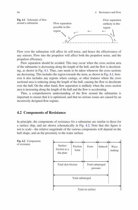
94 4 Resistance and Flow
Flow over the submarine will affect its self-noise, and hence the effectiveness of any sensors. Flow into the propulsor will affect both the propulsor noise, and the propulsor efficiency.
Flow separation should be avoided. This may occur when the cross section area of the submarine is decreasing along the length of the hull, and the flow is decelerat-ing, as shown in Fig. 4.1. Thus, care needs to be taken whenever the cross sections are decreasing. This includes the region towards the stern, as shown in Fig. 4.1, how-ever it also includes any regions where casings, or other features where the cross sectional area is reducing along the length of the hull, causing the flow to decelerate over the hull. On the other hand, flow separation is unlikely when the cross section area is increasing along the length of the hull and the flow is accelerating.
Thus, a comprehensive understanding of the flow around the submarine is important to ensure that it is optimised, and that no serious issues are caused by an incorrectly designed flow regime.
4.2 Components of Resistance
In principle, the components of resistance for a submarine are similar to those for a surface ship, and are shown schematically in Fig. 4.2. Note that this figure is not to scale—the relative magnitude of the various components will depend on the hull shape, and on the proximity to the water surface.
Fig. 4.1 Schematic of flow around a submarine Flow separation
possible in this region
Flow separationunlikely in this region
Fig. 4.2 Components of resistance Surface
friction as a flat plate
Friction form
Form Induced Wave making
Total skin friction Total submerged pressure
Total submerged
Total on surface
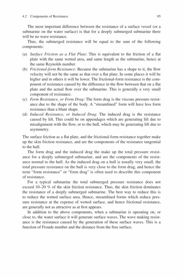
95
The most important difference between the resistance of a surface vessel (or a submarine on the water surface) is that for a deeply submerged submarine there will be no wave resistance.
Thus, the submerged resistance will be equal to the sum of the following components:
(a) Surface Friction as a Flat Plate: This is equivalent to the friction of a flat plate with the same wetted area, and same length as the submarine, hence at the same Reynolds number.
(b) Frictional-form Resistance: Because the submarine has a shape to it, the flow velocity will not be the same as that over a flat plate. In some places it will be higher and in others it will be lower. The frictional-form resistance is the com-ponent of resistance caused by the difference in the flow between that on a flat plate and the actual flow over the submarine. This is generally a very small component of resistance.
(c) Form Resistance, or Form Drag: The form drag is the viscous pressure resist-ance due to the shape of the body. A “streamlined” form will have less form resistance than a blunt shape.
(d) Induced Resistance, or Induced Drag: The induced drag is the resistance caused by lift. This could be on appendages which are generating lift due to misalignment with the flow, or to the hull, which may be generating lift due to asymmetry.
The surface friction as a flat plate, and the frictional-form resistance together make up the skin friction resistance, and are the components of the resistance tangential to the hull.
The form drag and the induced drag the make up the total pressure resist-ance for a deeply submerged submarine, and are the components of the resist-ance normal to the hull. As the induced drag on a hull is usually very small, the total pressure resistance on the hull is very close to the form drag, and hence the term “form resistance” or “form drag” is often used to describe this component of resistance.
For a typical submarine the total submerged pressure resistance does not exceed 10–20 % of the skin friction resistance. Thus, the skin friction dominates the resistance of a deeply submerged submarine. The best way to reduce this is to reduce the wetted surface area. Hence, streamlined forms which reduce pres-sure resistance at the expense of wetted surface, and hence frictional resistance, are generally not as attractive as at first appears.
In addition to the above components, when a submarine is operating on, or close to, the water surface it will generate surface waves. The wave making resist-ance is the resistance caused by the generation of these surface waves. This is a function of Froude number and the distance from the free surface.
4.2 Components of Resistance

96 4 Resistance and Flow
4.3 Effect of Hull Form
The optimal bare hull form is an axisymmetric body with a longitudinal section similar to a teardrop, as shown in Fig. 4.3. The fullest section is approximately 30–40 % aft of the bow, however this is not critical. This is known as a teardrop hull form.
For a given volume, increasing elongation decreases form resistance but increases frictional resistance. A circular cross section gives the lowest wetted area, and hence the lowest frictional resistance. Casings and other features which increase the wetted area will increase the frictional resistance.
The following two parameters are important when considering the overall shape of the hull form:
(a) slenderness ratio = L/D, where L is the submarine length, and D is its diam-eter; and
(b) prismatic coefficient, Cp = ∇AmL
, where ∇ is the volume of the submarine and Am is its midships cross sectional area.
The drag coefficient is plotted as a function of L/D for an axisymmetric teardrop hull in Fig. 4.4, developed using CFD. The relative size of the skin friction resist-ance and the form drag can be seen from this figure.
As can be seen from this figure, for larger values of L/D, although the form drag is smaller, the skin friction resistance is greater.
Fig. 4.3 Schematic of axisymmetric teardrop hull form
Fig. 4.4 Resistance components for an axisymmetric teardrop hull form
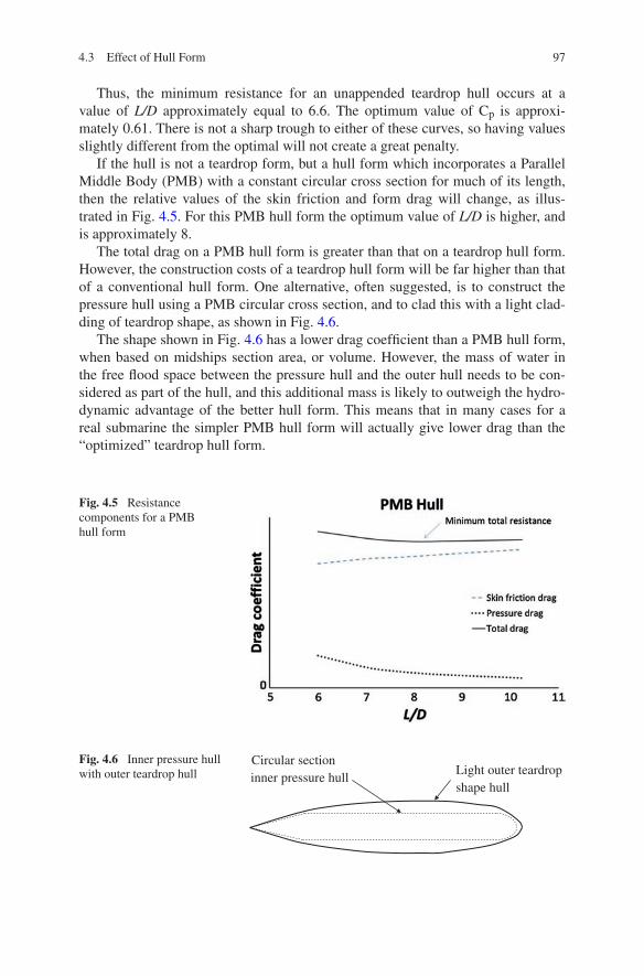
97
Thus, the minimum resistance for an unappended teardrop hull occurs at a value of L/D approximately equal to 6.6. The optimum value of Cp is approxi-mately 0.61. There is not a sharp trough to either of these curves, so having values slightly different from the optimal will not create a great penalty.
If the hull is not a teardrop form, but a hull form which incorporates a Parallel Middle Body (PMB) with a constant circular cross section for much of its length, then the relative values of the skin friction and form drag will change, as illus-trated in Fig. 4.5. For this PMB hull form the optimum value of L/D is higher, and is approximately 8.
The total drag on a PMB hull form is greater than that on a teardrop hull form. However, the construction costs of a teardrop hull form will be far higher than that of a conventional hull form. One alternative, often suggested, is to construct the pressure hull using a PMB circular cross section, and to clad this with a light clad-ding of teardrop shape, as shown in Fig. 4.6.
The shape shown in Fig. 4.6 has a lower drag coefficient than a PMB hull form, when based on midships section area, or volume. However, the mass of water in the free flood space between the pressure hull and the outer hull needs to be con-sidered as part of the hull, and this additional mass is likely to outweigh the hydro-dynamic advantage of the better hull form. This means that in many cases for a real submarine the simpler PMB hull form will actually give lower drag than the “optimized” teardrop hull form.
Fig. 4.5 Resistance components for a PMB hull form
Fig. 4.6 Inner pressure hull with outer teardrop hull
Circular section inner pressure hull
Light outer teardrop shape hull
4.3 Effect of Hull Form
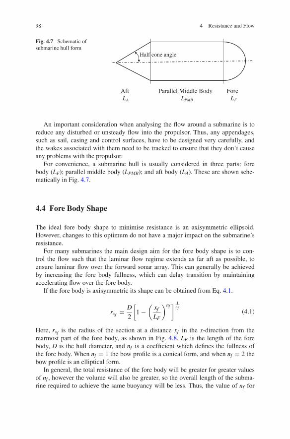
98 4 Resistance and Flow
An important consideration when analysing the flow around a submarine is to reduce any disturbed or unsteady flow into the propulsor. Thus, any appendages, such as sail, casing and control surfaces, have to be designed very carefully, and the wakes associated with them need to be tracked to ensure that they don’t cause any problems with the propulsor.
For convenience, a submarine hull is usually considered in three parts: fore body (LF); parallel middle body (LPMB); and aft body (LA). These are shown sche-matically in Fig. 4.7.
4.4 Fore Body Shape
The ideal fore body shape to minimise resistance is an axisymmetric ellipsoid. However, changes to this optimum do not have a major impact on the submarine’s resistance.
For many submarines the main design aim for the fore body shape is to con-trol the flow such that the laminar flow regime extends as far aft as possible, to ensure laminar flow over the forward sonar array. This can generally be achieved by increasing the fore body fullness, which can delay transition by maintaining accelerating flow over the fore body.
If the fore body is axisymmetric its shape can be obtained from Eq. 4.1.
Here, rxf is the radius of the section at a distance xf in the x-direction from the rearmost part of the fore body, as shown in Fig. 4.8. LF is the length of the fore body, D is the hull diameter, and nf is a coefficient which defines the fullness of the fore body. When nf = 1 the bow profile is a conical form, and when nf = 2 the bow profile is an elliptical form.
In general, the total resistance of the fore body will be greater for greater values of nf , however the volume will also be greater, so the overall length of the subma-rine required to achieve the same buoyancy will be less. Thus, the value of nf for
(4.1)rxf =D
2
[
1−(
xf
LF
)nf]
1nf
Fig. 4.7 Schematic of submarine hull form
Aft Parallel Middle Body ForeLA LPMB LF
Half cone angle
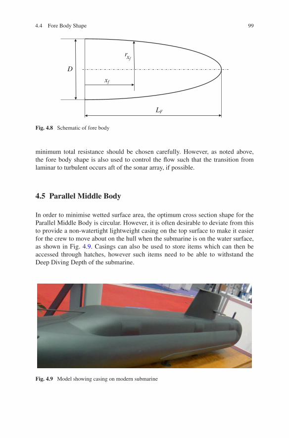
99
minimum total resistance should be chosen carefully. However, as noted above, the fore body shape is also used to control the flow such that the transition from laminar to turbulent occurs aft of the sonar array, if possible.
4.5 Parallel Middle Body
In order to minimise wetted surface area, the optimum cross section shape for the Parallel Middle Body is circular. However, it is often desirable to deviate from this to provide a non-watertight lightweight casing on the top surface to make it easier for the crew to move about on the hull when the submarine is on the water surface, as shown in Fig. 4.9. Casings can also be used to store items which can then be accessed through hatches, however such items need to be able to withstand the Deep Diving Depth of the submarine.
D
rxf
xf
LF
Fig. 4.8 Schematic of fore body
Fig. 4.9 Model showing casing on modern submarine
4.4 Fore Body Shape

100 4 Resistance and Flow
As shown in Fig. 4.5 the optimum L/D for a submarine with a PMB hull form is approximately 8. However, an increased L/D will result in a smaller diameter for a given volume, which can be cheaper to construct.
It is also worth bearing in mind that if the L/D value is too small then larger appendages may be required to maintain control. As appendages contribute sub-stantially to the resistance (Chap. 6), then this may suggest that a larger value of L/D should be chosen.
4.6 Aft Body Shape
The principal feature of the aft body is the half tail cone angle, as defined in Fig. 4.7. Too long an aft body, with a low half cone angle, will result in increased wetted surface (hence greater skin friction resistance), increased weight and greater cost. On the other hand, if the aft body is too short, with a large half cone angle then it may cause the flow to separate which, in addition to increasing the self-noise and drag on the hull, will cause disturbed flow to enter the propulsor, and result in a considerable increase in propulsor noise.
The aft body needs to be considered in conjunction with the propulsor, as discussed in Sect. 5.1. For a single propulsor on the hull’s axis the presence of the propulsor will result in an accelerating flow, as illustrated schematically in Fig. 4.10. As noted above, separation is less likely when the flow is accelerating. This means that the ideal form of the aft body without such a propulsor will be dif-ferent to that with one. The presence of the propulsor will permit a higher half tail cone angle and a fuller aft body, as discussed by Warren and Thomas (2000).
The normal arrangement for a single propulsor on a modern submarine is with the control appendages ahead of the propulsor, as shown in Fig. 4.11. The axisym-metric arrangement also allows a large diameter low speed propulsor which means that the propulsor efficiency can be very high—see Chap. 5.
In addition to the effect of the propulsor on the flow around the hull, the hull will affect the flow into the propulsor. This is due to:
(a) wake caused by the body ahead of the propulsor; and(b) thrust deduction due to the low pressure ahead of the propulsor.
Fig. 4.10 Schematic illustrating flow being accelerated into propulsor
Flow accelerating into propulsor

101
The hull efficiency, ηH, is the ratio of effective power to thrust power as discussed in sub Sect. 5.1.4. This is defined by Eq. 4.2.
where t is the thrust deduction fraction, and w is the Taylor wake fraction (Sect. 5.2). The full aft body will generate a high wake, which can result in hull efficiency values above 1.
The longitudinal position of the propulsor is not very critical to its perfor-mance, however it is desirable to have a reasonable separation between the pro-pulsor and the appendages, as the disturbed flow from the appendages will create uneven flow into the propulsor, and generate propulsor noise.
In addition to accelerating the flow in the axial direction, a propulsor will also accelerate it in a rotational direction, which is lost energy, thus reducing its efficiency (sub Sect. 5.1.5). Surface ships often have the propeller immediately behind the rud-der, thus reducing the lost energy due to rotational flow, but this is not the case for most submarines. Reducing rotational losses is one reason for adopting the pump-jet propulsor system, as discussed in Chap. 5. It is possible to reduce the rotational losses caused by the propeller by fitting stators ahead of the propeller. See Chap. 5.
4.7 Operating Close to the Surface
When operating close to the water surface a submarine will generate surface waves, and hence wave resistance. This will depend on the Froude number (Fr) and the submergence of the submarine, (H*). As the sail will be close to the sur-face, and potentially generating the most significant wave pattern, the Froude number based on the chord of the sail should be considered, in addition to the Froude number based on the length of the hull.
(4.2)ηH =(1− t)
(1− w)
Fig. 4.11 Typical aft arrangement of propulsor and control appendages
4.6 Aft Body Shape
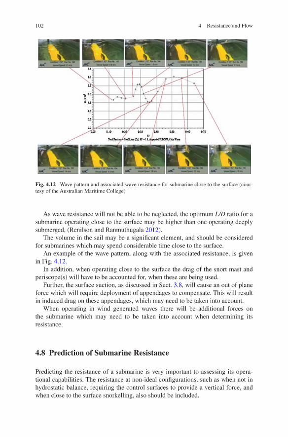
102 4 Resistance and Flow
As wave resistance will not be able to be neglected, the optimum L/D ratio for a submarine operating close to the surface may be higher than one operating deeply submerged, (Renilson and Ranmuthugala 2012).
The volume in the sail may be a significant element, and should be considered for submarines which may spend considerable time close to the surface.
An example of the wave pattern, along with the associated resistance, is given in Fig. 4.12.
In addition, when operating close to the surface the drag of the snort mast and periscope(s) will have to be accounted for, when these are being used.
Further, the surface suction, as discussed in Sect. 3.8, will cause an out of plane force which will require deployment of appendages to compensate. This will result in induced drag on these appendages, which may need to be taken into account.
When operating in wind generated waves there will be additional forces on the submarine which may need to be taken into account when determining its resistance.
4.8 Prediction of Submarine Resistance
Predicting the resistance of a submarine is very important to assessing its opera-tional capabilities. The resistance at non-ideal configurations, such as when not in hydrostatic balance, requiring the control surfaces to provide a vertical force, and when close to the surface snorkelling, also should be included.
Fig. 4.12 Wave pattern and associated wave resistance for submarine close to the surface (cour-tesy of the Australian Maritime College)

103
It is also necessary to be able to predict accurately the resistance of a submarine to design the propulsor.
The resistance of a submarine can be determined either by model testing, or by Computational Fluid Dynamics (CFD). For a deeply submerged submarine there will be no wave resistance, so the total resistance is made up of pressure resistance (primarily form drag) and frictional resistance. As noted in Figs. 4.4 and 4.5 the form drag is only a small component of the total. To estimate resistance it is neces-sary to consider full scale Reynolds number, if possible.
4.8.1 Model Testing
4.8.1.1 Resistance When Deeply Submerged
The normal method for predicting the resistance of a deeply submerged subma-rine is to test it in a towing tank as illustrated in Fig. 4.13. The model is supported by struts and tested inverted to reduce the interference caused by the struts. It is generally tested as deep as possible to avoid free surface effects, however it is also necessary to avoid any influence from the bottom of the tank. This approach allows for an operating propulsor if required for self-propulsion tests.
As it is not possible to achieve the full scale Reynolds number, and Froude number is not relevant to the resistance of a deeply submerged submarine, the procedure is generally to test at as high a speed as convenient, without generat-ing significant surface waves. Most hydrodynamics facilities will have a standard speed at which they test.
As is the case when testing models of surface ships the Reynolds number at model scale will be much lower than that at full scale so the flow over the model will be partly laminar. As with surface ship models, turbulent flow is achieved using turbulence stimulation close to the bow, and each hydrodynamic facility will have its own procedure for this. However, ensuring turbulent flow over the append-ages, particularly the hydroplanes and rudders, is difficult since the Reynolds numbers over these can be quite small. Overly large turbulence stimulators will affect the flow and can result in excessive stimulator drag. This is one reason why
Fig. 4.13 Typical arrangement for testing the resistance of a submarine in a towing tank
4.8 Prediction of Submarine Resistance

104 4 Resistance and Flow
large models are preferred, as even with 5 m long models the size of the hydro-planes and rudders are small enough to result in very low Reynolds numbers at speeds normally possible in a towing tank.
One of the main problems with this approach is in determining the correlation between the results from the model test and the resistance of the full scale sub-marine. A similar problem exists for surface ships, however in that case there are a large number of well documented full scale trials results, which can be used to develop a reliable correlation between the model test and the full scale. Of course this correlation only applies to that particular model test facility, using its standard test procedure.
The problem with trying to predict the resistance of a submarine is the lack of a large range of full scale trials data on different hull shapes. Thus, determining the empirical correlation allowance for submarines is difficult, and care needs to be taken with the results from the model experiment. Such issues include:
(a) strut interference on the model test;(b) blockage and wave resistance in towing tank;(c) level of turbulent flow on the model, particularly the appendages; and(d) additional drag on the full scale due to holes/vents for the ballast tanks and
other imperfections on the hull.
Another approach for determining the resistance of a deeply submerged submarine is to make use of physical model tests in a wind tunnel. Depending on the size, and top speed available, it may be possible to obtain a higher Reynolds number in a wind tunnel than a towing tank. In addition, there are no complications with the
Fig. 4.14 Submarine model being tested for resistance in a wind tunnel (courtesy of DSTO)

105
generation of surface waves, and it is easier to make modifications to the model during the testing program. Flow visualisation is also easier to achieve. A photo-graph of a model being tested in a wind tunnel is given in Fig. 4.14.
4.8.1.2 Resistance Close to the Water Surface
In order to obtain the resistance of a submarine when operating close to the water surface it is necessary to conduct model tests in a towing tank with the model upright. Testing inverted is no longer applicable as interaction between the sail and the water surface is one of the aspects being investigated.
This can cause additional problems. As can be seen in Fig. 4.15, using the two strut approach when close to the surface could result in considerable interference with the sail.
Alternatives are to use the aft sting support, as shown in Fig. 4.16, or a single strut through the sail, as shown in Fig. 4.17. Note that in both cases great care needs to be taken to ensure that the test rig is sufficiently stiff. This is particu-larly the case with the aft sting support. With the aft sting support it is not possible to test with an operating propulsor. As noted in Sect. 4.6 a propulsor can signifi-cantly affect the flow over the aft body, meaning that the optimum shape without a propulsor is different to that with a propulsor. However, this technique may be
Fig. 4.15 Schematic of submarine being tested close to the surface using the two strut system
Fig. 4.16 Schematic of submarine being tested close to the surface using an aft sting support
4.8 Prediction of Submarine Resistance
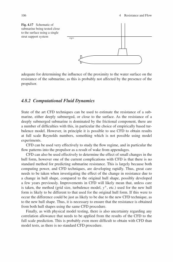
106 4 Resistance and Flow
adequate for determining the influence of the proximity to the water surface on the resistance of the submarine, as this is probably not affected by the presence of the propulsor.
4.8.2 Computational Fluid Dynamics
State of the art CFD techniques can be used to estimate the resistance of a sub-marine, either deeply submerged, or close to the surface. As the resistance of a deeply submerged submarine is dominated by the frictional component, there are a number of difficulties with this, in particular the choice of empirically based tur-bulence model. However, in principle it is possible to use CFD to obtain results at full scale Reynolds numbers, something which is not possible using model experiments.
CFD can be used very effectively to study the flow regime, and in particular the flow patterns into the propulsor as a result of wake from appendages.
CFD can also be used effectively to determine the effect of small changes in the hull form, however one of the current complications with CFD is that there is no standard method for predicting submarine resistance. This is largely because both computing power, and CFD techniques, are developing rapidly. Thus, great care needs to be taken when investigating the effect of the change in resistance due to a change in hull shape, compared to the original hull shape, possibly developed a few years previously. Improvements in CFD will likely mean that, unless care is taken, the method (grid size, turbulence model, y+, etc.) used for the new hull form is likely to be different to that used for the original hull form. If this were to occur the difference could be just as likely to be due to the new CFD technique, as to the new hull shape. Thus, it is necessary to ensure that the resistance is obtained from both hull shapes using the same CFD procedure.
Finally, as with physical model testing, there is also uncertainty regarding any correlation allowance that needs to be applied from the results of the CFD to the full scale prediction. This is probably even more difficult to obtain with CFD than model tests, as there is no standard CFD procedure.
Fig. 4.17 Schematic of submarine being tested close to the surface using a single strut support system
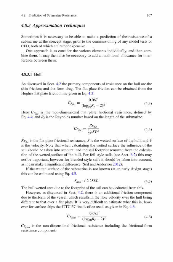
107
4.8.3 Approximation Techniques
Sometimes it is necessary to be able to make a prediction of the resistance of a submarine at the concept stage, prior to the commissioning of any model tests or CFD, both of which are rather expensive.
One approach is to consider the various elements individually, and then com-bine them. It may then also be necessary to add an additional allowance for inter-ference between them.
4.8.3.1 Hull
As discussed in Sect. 4.2 the primary components of resistance on the hull are the skin friction; and the form drag. The flat plate friction can be obtained from the Hughes flat plate friction line given in Eq. 4.3.
Here CFflat is the non-dimensional flat plate frictional resistance, defined by Eq. 4.4, and Re is the Reynolds number based on the length of the submarine.
RFflat is the flat plate frictional resistance, S is the wetted surface of the hull, and V is the velocity. Note that when calculating the wetted surface the influence of the sail should be taken into account, and the sail footprint removed from the calcula-tion of the wetted surface of the hull. For foil style sails (see Sect. 6.2) this may not be important, however for blended style sails it should be taken into account, as it can make a significant difference (Seil and Anderson 2012).
If the wetted surface of the submarine is not known (at an early design stage) this can be estimated using Eq. 4.5.
The hull wetted area due to the footprint of the sail can be deducted from this.However, as discussed in Sect. 4.2, there is an additional friction component
due to the form of the vessel, which results in the flow velocity over the hull being different to that over a flat plate. It is very difficult to estimate what this is, how-ever for surface ships the ITTC’57 line is often used, as given in Eq. 4.6.
CFform is the non-dimensional frictional resistance including the frictional-form resistance component.
(4.3)CFflat =0.067
(log10Re − 2)2
(4.4)CFflat =RFflat
12ρSV2
(4.5)Shull ≈ 2.25LD
(4.6)CFform =0.075
(log10Re − 2)2
4.8 Prediction of Submarine Resistance
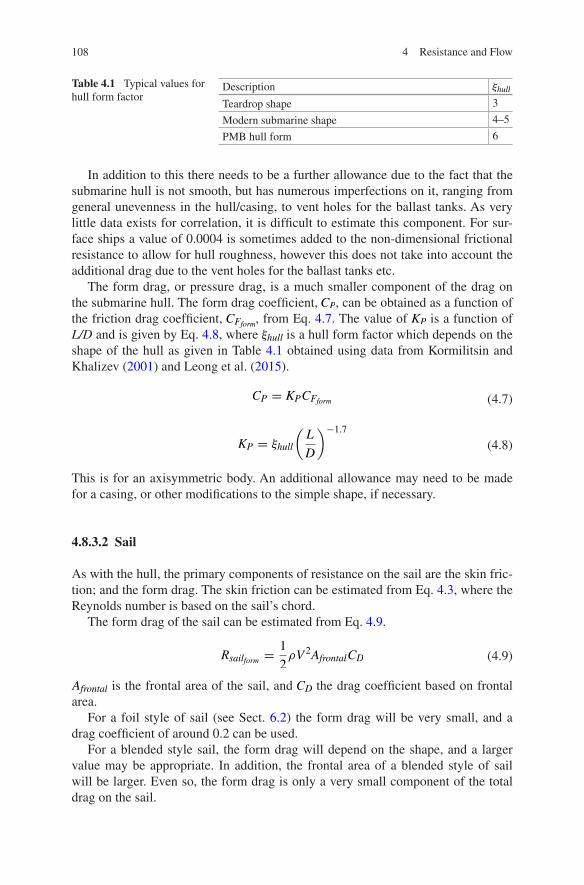
108 4 Resistance and Flow
In addition to this there needs to be a further allowance due to the fact that the submarine hull is not smooth, but has numerous imperfections on it, ranging from general unevenness in the hull/casing, to vent holes for the ballast tanks. As very little data exists for correlation, it is difficult to estimate this component. For sur-face ships a value of 0.0004 is sometimes added to the non-dimensional frictional resistance to allow for hull roughness, however this does not take into account the additional drag due to the vent holes for the ballast tanks etc.
The form drag, or pressure drag, is a much smaller component of the drag on the submarine hull. The form drag coefficient, CP, can be obtained as a function of the friction drag coefficient, CFform, from Eq. 4.7. The value of KP is a function of L/D and is given by Eq. 4.8, where ξhull is a hull form factor which depends on the shape of the hull as given in Table 4.1 obtained using data from Kormilitsin and Khalizev (2001) and Leong et al. (2015).
This is for an axisymmetric body. An additional allowance may need to be made for a casing, or other modifications to the simple shape, if necessary.
4.8.3.2 Sail
As with the hull, the primary components of resistance on the sail are the skin fric-tion; and the form drag. The skin friction can be estimated from Eq. 4.3, where the Reynolds number is based on the sail’s chord.
The form drag of the sail can be estimated from Eq. 4.9.
Afrontal is the frontal area of the sail, and CD the drag coefficient based on frontal area.
For a foil style of sail (see Sect. 6.2) the form drag will be very small, and a drag coefficient of around 0.2 can be used.
For a blended style sail, the form drag will depend on the shape, and a larger value may be appropriate. In addition, the frontal area of a blended style of sail will be larger. Even so, the form drag is only a very small component of the total drag on the sail.
(4.7)CP = KPCFform
(4.8)KP = ξhull
(
L
D
)−1.7
(4.9)Rsailform =1
2ρV2AfrontalCD
Table 4.1 Typical values for hull form factor
Description ξhull
Teardrop shape 3
Modern submarine shape 4–5
PMB hull form 6

109
4.8.3.3 Control Surfaces
As a first approximation Eq. 4.10 can be used to estimate the drag on the control surfaces.
The value of CD will depend on the design, as well as the aspect ratio, of the con-trol surfaces. A value of 0.01–0.02 can be used as a first estimate assuming that the control surfaces are aligned with the flow. If they are operating at an angle to the flow (as may be required due to the three dimensional nature of the flow around the submarine—Sect. 6.3) then an additional allowance for induced drag due to the lift generated will be required.
4.8.3.4 Interaction Effects
The total drag on the submarine can be obtained by adding the various compo-nents discussed above, however an allowance may need to be made for the addi-tional drag due to the interference between the various elements.
References
Kormilitsin YN, Khalizev OA (2001) Theory of submarine design. Saint Petersburg State Maritime Technical University, Russia
Leong ZQ, Ranmuthugala D, Renilson MR (2015) Resistance as a function of L/D ratio char-acteristics for various axisymmetrical hull forms. Australian Maritime College, Tasmania, Australia
Renilson MR, Ranmuthugala D (2012) The effect of proximity to free surface on the optimum length/diameter ratio for a submarine. In: First international conference on submarine technol-ogy and marine robotics (STaMR 2012), Chennai, 13–14 Jan 2012
Seil GJ, Anderson B (2012) A comparison of submarine fin geometry on the performance of a generic submarine. In: Proceedings of Pacific 2012 international maritime conference, Sydney, 2012
Warren CL, Thomas MW (2000) Submarine hull form optimisation case study. Naval Eng J 112(6):27–39
(4.10)Rcontrol surface =1
2ρV2AplanCD
4.8 Prediction of Submarine Resistance
111
Abstract The efficiency and acoustic performance of any propulsor will be affected by the flow into it. This is determined by: the hull shape, particularly the aft body and the tail cone angle; the casing; the sail; and the aft appendages. There will be an uneven wake field into the propulsor which will depend on the sail design and aft control surface configuration. This will result in fluctuating forces, causing vibra-tion and noise. Results are presented to estimate the Taylor wake fraction, and the thrust deduction fraction as functions of the tail cone angle and the ratio of propeller diameter to hull diameter. The hull efficiency, which is the ratio of effective power to thrust power, can be estimated. The relative rotative efficiency is the ratio of the open water propulsive efficiency to the efficiency of the propulsor when operating in the wake. The Quasi Propulsive Coefficient (QPC) is the ratio of useful power to the power delivered to the propeller. Submarines are often propelled by a large opti-mum diameter single propeller. It is important to avoid cavitation, and the Cavitation Inception Speed depends on depth of submergence. Blade number is important, and this is discussed. Many submarines use pumpjets, which comprise two or more blade rows within a duct. The principles of pumpjets are discussed, along with some design guidance. The diameter of a pumpjet is usually smaller than that of a propel-ler, resulting in a lower rotor tip speed. Contra-rotating propulsion; twin propellers; podded propulsion; and rim driven propulsion are also discussed.
Keywords Propeller · Pumpjet · Wake · Thrust deduction · Cavitation inception speed · Quasi propulsive coefficient
5.1 Propulsor/Hull Interaction
5.1.1 Flow into the Propulsor
The efficiency and acoustic performance of any propulsor will be significantly affected by the inflow to it. This is determined by: the shape of the hull, particularly
Chapter 5Propulsion
© The Author(s) 2015 M. Renilson, Submarine Hydrodynamics, SpringerBriefs in Applied Sciences and Technology, DOI 10.1007/978-3-319-16184-6_5

112 5 Propulsion
the aft body and the tail cone angle; the presence and size of any casing; the shape and size of the sail; and the size and configuration of the aft appendages.
The propulsor will experience different flow conditions when operating behind the submarine as compared to when it is in open water without the presence of the submarine ahead of it. This is caused by the wake of the submarine which has a major effect on the propulsor. In principle the wake is very similar to that for sur-face ships.
The effect of the wake into the propulsor is illustrated schematically in Fig. 5.1. In this figure a contour of constant velocity is shown. The velocity inboard of the contour line is lower than that on the contour line, and the velocity outboard of it is higher.
The left hand side of the figure shows an X-form shape, with the contour of constant velocity shown as a dashed line. As can be seen, there is a slightly lower velocity at the top, caused by the wake from the sail. There is also a lower velocity in line with the two hydroplanes.
The right hand side of the figure shows a cruciform shape, with the contour of constant velocity shown as a full line. As can be seen, there is a considerably lower velocity at the top, caused by the sail and the upper rudder. There is also a lower velocity at the side in the wake of the horizontal stabilizer, and at the bottom, in line with the lower rudder.
Fig. 5.1 Schematic of wake at the propulsor plane (left hand side illustrates X-form and right hand side illustrates cruciform)
Constant velocity contour
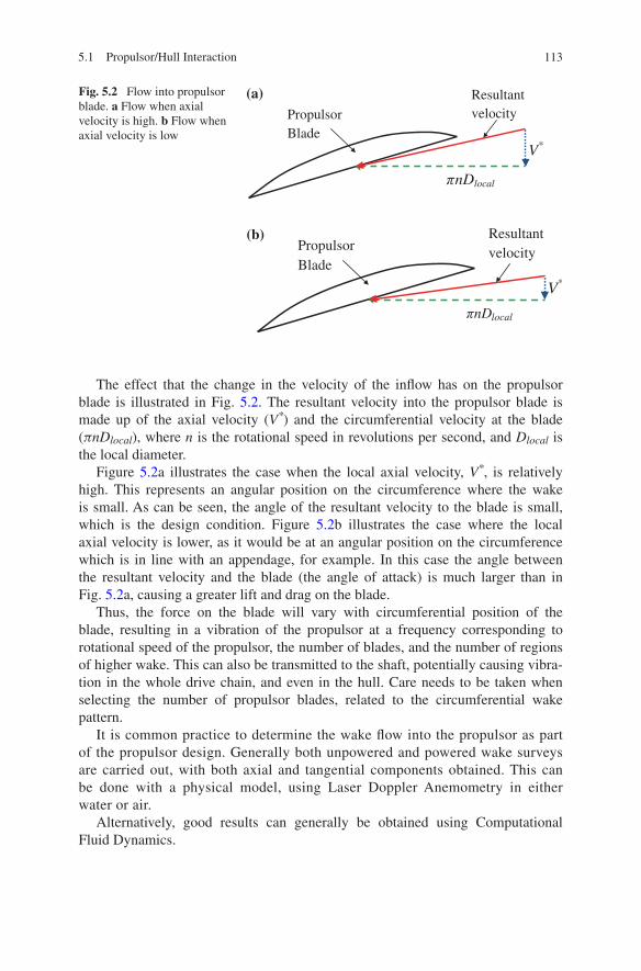
113
The effect that the change in the velocity of the inflow has on the propulsor blade is illustrated in Fig. 5.2. The resultant velocity into the propulsor blade is made up of the axial velocity (V*) and the circumferential velocity at the blade (πnDlocal), where n is the rotational speed in revolutions per second, and Dlocal is the local diameter.
Figure 5.2a illustrates the case when the local axial velocity, V*, is relatively high. This represents an angular position on the circumference where the wake is small. As can be seen, the angle of the resultant velocity to the blade is small, which is the design condition. Figure 5.2b illustrates the case where the local axial velocity is lower, as it would be at an angular position on the circumference which is in line with an appendage, for example. In this case the angle between the resultant velocity and the blade (the angle of attack) is much larger than in Fig. 5.2a, causing a greater lift and drag on the blade.
Thus, the force on the blade will vary with circumferential position of the blade, resulting in a vibration of the propulsor at a frequency corresponding to rotational speed of the propulsor, the number of blades, and the number of regions of higher wake. This can also be transmitted to the shaft, potentially causing vibra-tion in the whole drive chain, and even in the hull. Care needs to be taken when selecting the number of propulsor blades, related to the circumferential wake pattern.
It is common practice to determine the wake flow into the propulsor as part of the propulsor design. Generally both unpowered and powered wake surveys are carried out, with both axial and tangential components obtained. This can be done with a physical model, using Laser Doppler Anemometry in either water or air.
Alternatively, good results can generally be obtained using Computational Fluid Dynamics.
Fig. 5.2 Flow into propulsor blade. a Flow when axial velocity is high. b Flow when axial velocity is low
nDlocal
V*
Resultant velocityPropulsor
Blade
nDlocal
V*
Resultant velocityPropulsor
Blade
(a)
(b)
5.1 Propulsor/Hull Interaction

114 5 Propulsion
5.1.2 Wake
The wake fraction, w, is defined by Eq. 5.1.
In this equation, w, is known as the Taylor wake fraction, V, is the vessel velocity, and Va is the velocity of advance of the propulsor.
The Taylor wake fraction will depend on the tail cone angle, and the ratio of propeller diameter to hull diameter, as shown in Fig. 5.3 adapted from Burcher and Rydill (1998). Note that the total tail cone angle (twice the half tail cone angle) is used in this figure.
5.1.3 Thrust Deduction
The other major effect that the propulsor will have is to generate a “pull” on the aft end of the submarine, due to the low pressures ahead of it. This is accounted for by assuming a deduction in thrust. The thrust deduction fraction, t, is given by Eq. 5.2.
(5.1)w =V − Va
V
(5.2)t =T − RT
T
Fig. 5.3 Taylor wake fraction (adapted from Burcher and Rydill 1998)

115
In this equation, t, is the thrust deduction fraction, T, is the propulsor thrust, and RT is the total hull resistance.
The thrust deduction fraction will depend on the tail cone angle, and the ratio of propeller diameter to hull diameter, as shown in Fig. 5.4, adapted from Burcher and Rydill (1998) and Kormilitsin and Khalizev (2001). Note that the total tail cone angle (twice the half tail cone angle) is used in this figure.
5.1.4 Hull Efficiency
The hull efficiency, ηH, is the ratio of the effective power to the thrust power. It is important to note that the hull efficiency is not efficiency as such, but the ratio of efficiencies. Thus, it is possible for the hull efficiency to be greater than one. Hull efficiency is defined in Eq. 5.3.
PE is the effective power; PT is the thrust power; t is the thrust deduction; and w is the Taylor wake fraction.
Using the data in Figs. 5.3 and 5.4 the hull efficiency obtained is given in Fig. 5.5. Note that the total tail cone angle (twice the half tail cone angle) is used in this figure. As can be seen, the hull efficiency is always greater than one. This is due to the high wake, compared to the thrust deduction fraction. At an early stage
(5.3)ηH =PE
PT
=(1− t)
(1− w)
Fig. 5.4 Thrust deduction (adapted from Burcher and Rydill 1998, and Kormilitsin and Khalizev 2001)
5.1 Propulsor/Hull Interaction

116 5 Propulsion
of the design this figure can be used to estimate the hull efficiency, however self-propelled model experiments would usually be used to refine this at a later stage in the design.
5.1.5 Relative Rotative Efficiency
The relative rotative efficiency, ηR, is the ratio of the open water propulsive effi-ciency, ηO, to the efficiency of the propulsor when operating in the wake behind the submarine. For a submarine with a single propulsor on the axis the value of ηR will depend on the shape of the aft body (characterized by the tail cone angle) and its appendages. It is also dependent on the ratio of the propeller diameter to hull diameter.
For values of the ratio of propeller diameter to hull diameter in the range of 0.4–0.7, and full tail cone angles of 20°–50°, ηR will be approximately 1.05, indi-cating that the propeller is more efficient when operating behind the submarine, than in open water. Part of the reason for this is the flow straightening effects of the appendages, which will reduce the losses due to swirl. It is possible to fit sta-tors ahead of the propeller to further reduce the rotational losses.
For small propeller diameters, and large tail cone angles, the value of ηR can reduce to below unity.
In the extreme case where the propeller diameter is much greater than the hull diameter, and the tail cone angle is small, then the value of ηR must tend to unity, as the propeller will be operating close to its open water condition.
Fig. 5.5 Hull efficiency (using data from Burcher and Rydill 1998)
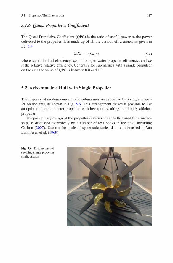
117
5.1.6 Quasi Propulsive Coefficient
The Quasi Propulsive Coefficient (QPC) is the ratio of useful power to the power delivered to the propeller. It is made up of all the various efficiencies, as given in Eq. 5.4.
where ηH is the hull efficiency; ηO is the open water propeller efficiency; and ηR is the relative rotative efficiency. Generally for submarines with a single propulsor on the axis the value of QPC is between 0.8 and 1.0.
5.2 Axisymmetric Hull with Single Propeller
The majority of modern conventional submarines are propelled by a single propel-ler on the axis, as shown in Fig. 5.6. This arrangement makes it possible to use an optimum large diameter propeller, with low rpm, resulting in a highly efficient propeller.
The preliminary design of the propeller is very similar to that used for a surface ship, as discussed extensively by a number of text books in the field, including Carlton (2007). Use can be made of systematic series data, as discussed in Van Lammeren et al. (1969).
(5.4)QPC = ηHηOηR
Fig. 5.6 Display model showing single propeller configuration
5.1 Propulsor/Hull Interaction
118 5 Propulsion
The principal dimensions of a propeller are:
(a) number of blades;(b) diameter;(c) pitch;(d) rotational speed; and(e) blade area.
The first requirement for a submarine propeller design is the selection of the blade number. This is based on the need to minimise the acoustic noise signature gen-erated by fluctuating forces on the propeller caused by it operating in the wake behind the submarine, as discussed in sub Sect. 5.1.1. As can be seen in Fig. 5.1, for a cruciform stern there are typically four areas of reduced flow around the cir-cumference, due to the presence of the hydroplanes and the sail/casing. Hence, a four bladed propeller would experience each blade suffering from the reduced inflow at the same time, causing considerable vibration and resulting hydro-acous-tic noise. Thus, four blades, or a blade number which is a multiple of four, should be avoided. With the X-form stern there are five such areas of reduced flow due to the wake, and hence five blades, or a multiple of them, should be avoided.
Ideally, as high a blade number as possible should be selected, which should be a prime number, to avoid possible harmonics. However, there are practical con-cerns with very high blade numbers, and so consequently it is common practice to use a seven bladed propeller.
Next the diameter, pitch and rotational speed are selected.For a submarine with a single propeller on its axis the propeller design is not
constrained by its diameter, making it possible to select the optimum diameter for the required thrust at a given rotational speed from an existing propeller series. The pitch can then be determined from such series data. This process is the same as for surface ships, and is discussed in a number of text books on the subject, including Carlton (2007).
Although the hub size is generally a lot larger for a submarine than for a surface ship, a propeller series developed for surface ships will generally give a satisfactory preliminary propeller design, and a good estimate of its efficiency, adequate for con-cept design studies etc. This is because the velocity over the propeller at the hub is much lower than that over the rest of the blade, so its contribution to the overall thrust and torque is generally small. However, if series data for a submarine propeller is available it would clearly be preferable to make use of that.
The required blade area is then selected to avoid cavitation. Too small a blade area will result in too great a load on the blade, and hence a poor cavitation performance.
When a submarine is running deep cavitation should not be a problem, as the substantial head will increase the pressure, and hence cavitation is very unlikely. However, when running close to the surface cavitation could be a problem for a propeller with insufficient blade area, particularly when operating in off design conditions, such as accelerating, turning, or braking. Generally, avoiding cavita-tion in operating conditions for an undamaged submarine propeller is not difficult.

119
Even when a large blade number is selected, each blade will be operating in the wake, and can suffer a change in loading due to the circumferential change in wake. This can cause vibration and hydro-acoustic noise. Thus, to attempt to smooth this out over each blade, a large amount of skew is generally adopted, as shown in the display model in Fig. 5.6. This means that only a section of the blade will be experiencing the low axial inflow at any one time, and hence the overall effect on the blade will be reduced. However, care needs to be taken with exces-sive skew to avoid unwanted flexure in the blades, and also large stresses in the blades when applying astern thrust.
Once the principal dimensions of the propeller have been selected it is possible to consider the design features which will further reduce acoustic noise signature. For example, suction and pressure-side cavitation can normally be avoided by a thicker section profile than used for a comparable propeller for a surface ship. In order to avoid tip-vortex and hub-vortex cavitation submarine propellers usually have a reduc-tion in loading at their tips and hubs. In addition, the trailing edge region needs careful design to reduce trailing edge noise. It is not sufficient simply to reduce singing, but the whole noise spectrum needs to be considered. Hence submarine propellers are not normally provided with anti-singing trailing edges. (Anderson et al. 2009).
To reduce rotational losses, pre-swirl stators can be fitted ahead of an open propeller. The design of these stators needs to be conducted in conjunction with the propeller design, and in particular the selection of the number of stators, and the interaction between the appendages, the stators, and the propeller needs to be considered carefully. However, the incorporation of well-designed stators with an open propeller has the potential to provide many of the advantages of a pumpjet at lower cost and weight. See Sect. 5.3.
An example of a submarine propeller, from HMS Trafalgar, is shown in Fig. 5.7.
This is a specialist field, which is generally very highly classified.
Fig. 5.7 Propeller from HMS Trafalgar
5.2 Axisymmetric Hull with Single Propeller

120 5 Propulsion
5.3 Axisymmetric Hull with Single Pumpjet
Pumpjets comprise two or more blade rows within a duct, which can either be rotating (rotor) or static (stator) blades. One of the design objectives is to use the stators to remove the rotational flow imparted by the rotors. This rotational flow, which is always present behind single propellers, represents hydrodynamic loss, as energy has been utilised to rotate the flow, which is not used to propel the vessel and this reduces the efficiency. A photograph of a pumpjet in the cavitation tunnel at SSPA is given in Fig. 5.8, taken from SSPA (1993), with permission.
The primary motivation for the design of pumpjets for application to subma-rines is to reduce the hydro-acoustic signature, however it is also claimed that it can have a higher efficiency (Vinton et al. 2005).
The pumpjet provides a means of controlling the flow velocities over the blades and enables a direct trade-off of cavitation performance with efficiency to be achieved. In addition, the duct acts as an end wall for the blades, therefore ena-bling them to be loaded out to their tips, resulting in a significant reduction in the propulsor diameter compared to an open propeller. This will result in a lower tip speed. However, the gap between the tip of the rotor blade and the duct becomes very important, as this is where cavitation could occur. Ideally the gap should be as small as possible.
A pumpjet can be designed with the stator row aft of the rotor row (post-swirl) or with the stator row ahead of the rotor row (pre-swirl) as shown in Fig. 5.9. A post-swirl pumpjet requires additional struts forward of the rotor to support the duct, as can be seen in Fig. 5.9a.
The stators in post-swirl pumpjets can contribute of the order of 25 % of the total propulsor thrust, reducing the required loading on the rotors, and hence their tendency to cavitate (Clarke 1988). In addition, the duct can be designed to decelerate the flow, hence increasing the pressure. Both these measures will help
Fig. 5.8 Pumpjet on submarine model in the cavitation tunnel at SSPA (photo by Sven Wessling, courtesy of SSPA, taken from: SSPA 1993)
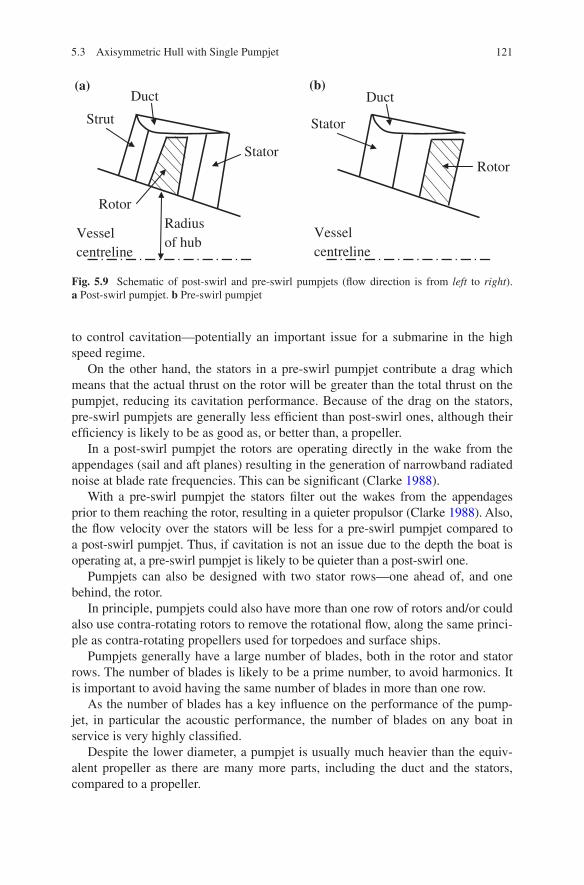
121
to control cavitation—potentially an important issue for a submarine in the high speed regime.
On the other hand, the stators in a pre-swirl pumpjet contribute a drag which means that the actual thrust on the rotor will be greater than the total thrust on the pumpjet, reducing its cavitation performance. Because of the drag on the stators, pre-swirl pumpjets are generally less efficient than post-swirl ones, although their efficiency is likely to be as good as, or better than, a propeller.
In a post-swirl pumpjet the rotors are operating directly in the wake from the appendages (sail and aft planes) resulting in the generation of narrowband radiated noise at blade rate frequencies. This can be significant (Clarke 1988).
With a pre-swirl pumpjet the stators filter out the wakes from the appendages prior to them reaching the rotor, resulting in a quieter propulsor (Clarke 1988). Also, the flow velocity over the stators will be less for a pre-swirl pumpjet compared to a post-swirl pumpjet. Thus, if cavitation is not an issue due to the depth the boat is operating at, a pre-swirl pumpjet is likely to be quieter than a post-swirl one.
Pumpjets can also be designed with two stator rows—one ahead of, and one behind, the rotor.
In principle, pumpjets could also have more than one row of rotors and/or could also use contra-rotating rotors to remove the rotational flow, along the same princi-ple as contra-rotating propellers used for torpedoes and surface ships.
Pumpjets generally have a large number of blades, both in the rotor and stator rows. The number of blades is likely to be a prime number, to avoid harmonics. It is important to avoid having the same number of blades in more than one row.
As the number of blades has a key influence on the performance of the pump-jet, in particular the acoustic performance, the number of blades on any boat in service is very highly classified.
Despite the lower diameter, a pumpjet is usually much heavier than the equiv-alent propeller as there are many more parts, including the duct and the stators, compared to a propeller.
Strut
Rotor
RotorStator
Duct
Stator
Duct
Radius of hub
Vessel centreline
Vessel centreline
(a) (b)
Fig. 5.9 Schematic of post-swirl and pre-swirl pumpjets (flow direction is from left to right). a Post-swirl pumpjet. b Pre-swirl pumpjet
5.3 Axisymmetric Hull with Single Pumpjet

122 5 Propulsion
The blades on the pumpjet are normally individually manufactured and attached to the hub. This results in a more complex hub than would be required for a fixed pitch propeller, meaning that the hub is likely to require a larger diameter. Hence, a pumpjet is likely to be mounted further forward on the submarine, where the hull diameter is greater. In addition, the larger mass of the pumpjet can cause a problem if placed too far aft, which is another reason for moving it forward com-pared to the location of a conventional propeller.
The primary parameter influencing cavitation performance is the blade area. Too small a blade area will result in too great a load on the blade, and hence a poor cavitation performance. If the diameter is small it will be difficult to provide sufficient blade area, and so the required blade area has a major influence on the pumpjet diameter necessary for cavitation performance.
A further important parameter is the rotor tip speed. Higher tip speeds will result in a higher possibility of tip-vortex cavitation, which is usually the type of cavitation which affects Cavitation Inception Speed (CIS). For a given propulsor rotational speed a larger diameter will result in a higher rotor tip speed.
The required diameter for a pumpjet will be smaller than that for an equivalent pro-peller, as the rotor tips can have higher loading due to the end wall provided by the duct.
Low propulsor rotational speed will improve both the cavitation and the acous-tic performance, however, lower rotational speed leads to the requirement for a larger diameter. Thus, the choice of rotational speed and diameter is a trade-off between cavitation and acoustic performance.
Depending on the design of the duct it can either accelerate or decelerate the flow through it. Schematic diagrams of the two extreme duct shapes are given in Fig. 5.10. For the accelerating duct the area at the inlet is greater than at the outlet, whereas for the decelerating duct the area at the inlet is smaller than at the outlet.
For designs with accelerating ducts, the duct can actually contribute to a positive thrust, increasing the efficiency of the rotor/duct combination. This concept is often
(a) (b)
Fig. 5.10 Schematic of accelerating and decelerating ducts (flow direction is from left to right). a Accelerating duct. b Decelerating duct

123
used for surface ships requiring high thrust at low speed, such as those engaged in towing operations. On the other hand, vessels with lower thrust and higher speed—hence lower propeller loading—do not normally benefit from an accelerating duct.
The higher water velocity over the blades when fitted with an accelerating duct will result in a lower pressure, and hence reduced cavitation performance.
Decelerating ducts reduce the water velocity over the blades, increasing the pressure, and hence can result in better cavitation performance. Against this, these ducts increase drag, resulting in the need for greater thrust from the blades, and decreasing efficiency.
The optimum duct shape for a submarine will depend on the propulsor loading, Bp, which is defined in Eq. 5.5.
where N is the revolutions per minute, PS is the power delivered to the shaft in horsepower, and Va is the velocity of advance of the propulsor in knots. As a rule of thumb for surface ships, a duct can be beneficial for Bp values greater than around 40 (Carlton 2007). Submarines generally have Bp values far smaller than this, implying that the duct itself would not be an advantage from a hydrodynamic point of view.
Both stator blades and rotor blades have aspect ratios much smaller than con-ventional open propellers. They do not have anything like the same level of skew that conventional submarine propellers have.
A well designed pumpjet will result in no rotational flow aft of the unit. As the rotational flow represents lost energy, there is the opportunity for pumpjets to have a higher efficiency than open propellers. On the other hand, the duct and the sta-tors (pre-swirl) can contribute to additional drag for typical values of propulsor loading associated with submarine operations, reducing efficiency. A value for efficiency of 0.833 is quoted for the design (post-swirl) in open water discussed by McCormick and Eisenhuth (1963). A pumpjet operating in the wake behind an axisymmetric body is likely to have a higher efficiency.
The astern performance of a pumpjet is much worse than a conventional open propeller. Part of the reason for the poor astern performance with a pump-jet is the duct design, and in particular the sharp trailing edge. Ducts for surface ships which are required to have good astern thrust performance, such as tugs, are designed with more rounded trailing edges, which reduce the efficiency in the ahead condition (Carlton 2007).
5.4 Other Configurations
5.4.1 Contra-rotating Propulsion
Contra-rotating propulsion consists of two propellers rotating in opposite direc-tions on the same shaft. The aft propeller recovers some of the rotational energy imparted by the forward propeller. Thus, in principle, the propulsive efficiency can be much greater than for a single propeller.
(5.5)Bp =NP0.5
S
V2.5a
5.3 Axisymmetric Hull with Single Pumpjet

124 5 Propulsion
Contra-rotating propulsion was used successfully on the USS Jack from 1967 to 1989, demonstrating a 10 % increase in propulsive efficiency (Dutton 1994).
As contra-rotating propulsion spreads the load over two propellers the blade loading is decreased, and hence cavitation is reduced. In addition, the propulsor rotational speed and/or the diameter can be reduced, again improving cavitation performance. However, not so much is known about the non-cavitating acous-tic performance of contra-rotating propulsion, and it is not commonly used for submarines.
On the other hand, contra-rotating propulsion has been common in the past for torpedo propulsion, as shown in Fig. 5.11. This is partly due to the reduction in the rolling moment that would be caused by a single propeller. However, modern tor-pedoes tend to use pumpjet propulsion, discussed in Sect. 5.3.
5.4.2 Twin Propellers
In some cases it is desirable to use twin propellers, which also improves the redun-dancy of the propulsion system. Examples of submarines which use twin screw propellers are the Russian Delta and Typhoon classes.
Changing from a single shaft to a twin shaft power plant of the same total out-put will result in an increase in nominal displacement of 10–20 % (Kormilitsin and Khalizev 2001).
As with all propulsion types, the inflow to the propellers is vital to their acous-tic performance. Thus, when twin propellers are being used on an axisymmetric submarine the inflow can be improved by flattening the after body, to result in a shape somewhat like that shown schematically in Fig. 5.12.
Fig. 5.11 Contra-rotating propellers on a MK 44 Torpedo
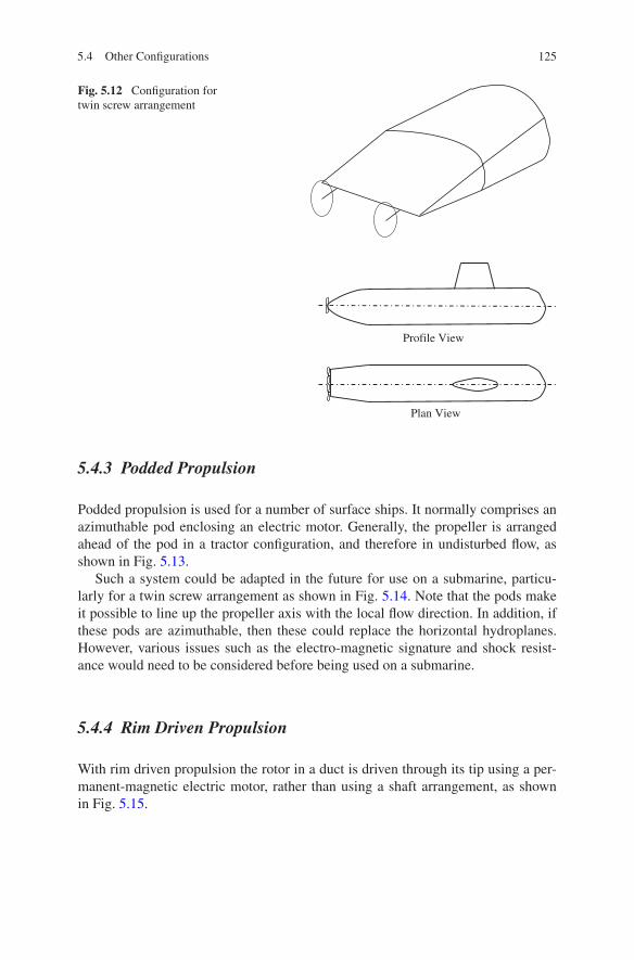
125
5.4.3 Podded Propulsion
Podded propulsion is used for a number of surface ships. It normally comprises an azimuthable pod enclosing an electric motor. Generally, the propeller is arranged ahead of the pod in a tractor configuration, and therefore in undisturbed flow, as shown in Fig. 5.13.
Such a system could be adapted in the future for use on a submarine, particu-larly for a twin screw arrangement as shown in Fig. 5.14. Note that the pods make it possible to line up the propeller axis with the local flow direction. In addition, if these pods are azimuthable, then these could replace the horizontal hydroplanes. However, various issues such as the electro-magnetic signature and shock resist-ance would need to be considered before being used on a submarine.
5.4.4 Rim Driven Propulsion
With rim driven propulsion the rotor in a duct is driven through its tip using a per-manent-magnetic electric motor, rather than using a shaft arrangement, as shown in Fig. 5.15.
Fig. 5.12 Configuration for twin screw arrangement
Profile View
Plan View
5.4 Other Configurations

126 5 Propulsion
The lack of a shaft improves the flow into the blades and hence can reduce vibration, and subsequent hydro-acoustic noise. In addition there is no gap between the outer edge of the rotor and the duct. This results in improved cavita-tion performance, compared to a shaft driven design, which must incorporate this gap. The inner portion of the rotor blades, which has the lowest velocity, is where the “tip” is, so the resulting vortices will be smaller in magnitude.
As the rotor is driven independently by its outer edge, contra-rotating rotors do not require the mechanical issues associated with a shaft, as discussed in sub Sect. 5.4.1. Also, the rotational speed of the different rotors can be independently controlled.
Finally, since the rotor is driven by a permanent-electric motor in the duct, it can be configured in a similar manner to a podded propulsor, and can be fully azimuthable, if required. Alternatively it can simply replace the single propulsor on the axis of an axisymmetrical hull shape.
Fig. 5.13 Podded propulsion for a surface ship
Fig. 5.14 Plan view of possible podded propulsion layout
Fig. 5.15 Typical rim driven propulsor (for a transverse thruster on a surface ship)
127
5.5 Prediction of Propulsor Performance
5.5.1 Physical Model Tests
5.5.1.1 Hydrodynamic Performance
As with surface ships, the prediction of the hydrodynamic performance of a sub-marine propulsor will involve both open water testing of a large scale propulsor, and the testing of a propulsor “behind” the submarine hull.
The former is often carried out in a cavitation tunnel. Cavitation must be com-pletely avoided on submarine propulsors, but as they usually operate at high pres-sure due to the large head of water, cavitation inception is not generally such an issue as with surface warships. Equally, it is not important to understand the behaviour of a submarine propulsor under cavitating conditions—as cavitation is completely avoided.
Tests to determine propulsor—hull interaction are conducted in a similar man-ner to those for a surface ship. The model is usually tested in a towing tank and is inverted using a two strut arrangement as shown in Fig. 4.13. Note that unlike surface ship tests Froude number is not important, so it is possible to conduct the tests at a single speed.
Tests are conducted at various different propulsor rpm, and the propulsor torque and thrust, and the hull resistance are measured. From this, the effective wake and the thrust deduction values at the full scale self-propulsion speed can be obtained, in a similar manner to that used for surface ships.
5.5.1.2 Hydro-acoustic Performance
As noted in Chap. 7, in addition to cavitation, hydro-acoustic noise can be narrow-band, or broadband.
Narrowband noise is due to the fluctuating loading on the propulsor blades, caused by the blades passing through the uneven wake field. Thus, in order to con-duct a physical model test to investigate narrowband noise it is necessary to test the propulsor in situ behind a model of the submarine hull, complete with all its appendages. Since the wake from the hull is dependent on Reynolds number, as large a Reynolds number as possible should be used. If the tests are conducted in a quiet water tunnel with a very low background noise, such as the tunnel operated by the French DGA shown in Fig. 5.16, then the noise at model scale can be meas-ured. Care is required to avoid self-noise on the hydrophones.
Broadband noise is due to turbulent interaction over the blade. Tests to deter-mine broadband noise are generally conducted at as large a scale as possible, often in “open water”, without a submarine hull. Again, a facility like that shown in Fig. 5.16 can be used.
5.5 Prediction of Propulsor Performance

128 5 Propulsion
As noted in Chap. 7, the fluctuating forces on the propulsor can set up reso-nances in the submarine, which in turn can generate radiated hydro-acoustic noise. To predict this noise it is necessary to measure the fluctuating forces in all three dimensions, and use this with a numerical model of the submarine shaft and rel-evant structure. To do this a sophisticated dynamometer is required, capable of measuring at very high frequencies. This is because, due to the scaling laws, model scale rpm is higher than full scale rpm, and it is necessary to capture the fluctuating forces at the higher harmonics. In addition, for a pumpjet the blade rate can be high, due to the number of stators and rotors.
5.5.2 Computational Fluid Dynamics
A range of Computational Fluid Dynamics (CFD) techniques exist which can be used for propulsor design. One of the simplest approaches is Reynolds-Averaged Navier-Stokes (RANS). The equations of motion of the flow are solved by split-ting it into time-averaged and fluctuating components. This approach usually makes use of an empirically derived turbulence model. At present (2015) a number of commercial RANS solvers exist, and the use of RANS is considered to be a fairly routine approach to the simulation of fluid flow.
RANS techniques can be used very effectively to determine the wake flow into the propulsor. As noted above, this is important for the design of the propulsor.
RANS can also be used to predict the hydrodynamic performance of the pro-pulsor itself, although at this time (2015) it is normal procedure, as a minimum, to conduct model experiments on the final design as confirmation.
As RANS can be used to predict both the wake field, and the propulsor hydro-dynamic performance, in principle it can also be used to predict the fluctuating forces on the blades, and hence the narrowband hydro-acoustic performance.
microbubblesgeneration
High pressure air
saturated water
Deaerated water
Downstream bubbles separating tank
air
LARGE TEST SECTION
Resorber
2 MW MOTOR
Main pump
Fig. 5.16 Hydroacoustic and cavitation tunnel GTH (courtesy of DGA Hydrodynamics)

129
However, at this time (2015) this is generally not considered accurate enough to have confidence in this approach without model tests.
As RANS relies on a simplification of the boundary layer flow, it is not pos-sible to use it to determine broadband hydro-acoustic noise. Further work is being undertaken using more sophisticated numerical approaches, however at this time (2015) the only reliable method of predicting broadband performance is by model testing as discussed above.
References
Andersen P, Kappel JJ, Spangenberg E (2009) Aspects of propeller developments for a subma-rine. In: First international symposium on marine propulsors, Trondheim, Norway, 2009
Burcher R, Rydill L (1998) Concepts in submarine design. Cambridge University Press, Cambridge
Carlton JS (2007) Marine propellers and propulsion. Elsevier, Oxford. ISBN: 978-07506-8150-6Clarke GE (1988) The choice of propulsor design for an underwater weapon. In: UDT confer-
ence, London, 26–28 Oct 1988Dutton JL, (1994) Contrarotating electric drive for attack submarines. Naval Eng J 106(2):45–50Kormilitsin YN, Khalizev OA (2001) Theory of submarine design. Saint Petersburg State
Maritime Technical University, RussiaMcCormick BW, Eisenhuth J (1963) Propellors and pumpjets for underwater propulsion. AIAA J
1(10):2348–2354SSPA (1993) Pumpjet propulsion. SSPA Highlights Mag 2:1993Van Lammeren WPA, Van Manen JD, Oosterveld MWC (1969) The Wageningen B screw series.
Soc Naval Archit Marine Eng Trans 77:269–317Vinton PM, Banks S, West M (2005) Astute propulsor technical innovation summary. In:
Proceedings of warship 2005—Naval submarines, Royal Institution of Naval Architects, London, 2005
5.5 Prediction of Propulsor Performance
131
Abstract Submarines usually have three groups of appendages: sail; forward control surfaces; and aft control surfaces. Appendages contribute a considerable increase in drag, and need to be considered carefully. There are two approaches to sail design: a foil type; and a blended type. The blended type of sail has a larger volume than the foil type, and is better faired into the hull. If the sail is at an angle of attack it will generate a side force high up resulting in a heel angle (particularly snap roll) and a force and moment in the vertical plane on the hull, resulting in a stern dipping tendency. The magnitude of the side force when manoeuvring will depend on the distance of the sail from the Pivot Point. The location of the sail will also affect the turning radius. The forward planes can be located in three dif-ferent positions: midline; eyebrow; and sail. The pros and cons of each of these are discussed. The aft control surfaces may include fixed and movable surfaces, with the fixed surfaces increasing stability, and the movable surfaces used to change trim, and hence to make large depth changes, and to turn the submarine. Different aft control surface configurations include: cruciform; X-form; inverted Y; and pen-taform. The pros and cons of these different configurations are discussed.
Keywords Propeller · Pumpjet · Wake · Thrust deduction · Cavitation Inception Speed · Quasi Propulsive Coefficient
6.1 General
Submarines usually have three groups of appendages as follows:
(a) sail—to house periscopes, snorkel, and other masts, as well as to serve as the conning position when on the surface;
(b) forward control surfaces—to permit the submarine to change depth without changing trim, and to control depth at low speeds; and
(c) aft control surfaces—to control depth by changing trim, and to provide steer-ing in the horizontal plane.
Chapter 6Appendage Design
© The Author(s) 2015 M. Renilson, Submarine Hydrodynamics, SpringerBriefs in Applied Sciences and Technology, DOI 10.1007/978-3-319-16184-6_6

132 6 Appendage Design
Appendages contribute a considerable increase in drag, and need to be consid-ered carefully. They will often operate at an angle to the flow, thereby resulting in induced drag, and associated vortices. Care needs to be taken to ensure that root fairing is done carefully, particularly over regions of the hull where the cross sec-tion is decreasing (see Sect. 4.1).
In addition, appendages need to be designed for the expected angle of the flow over them.
The size of the control surfaces may be dictated by the need to control depth when at periscope depth in waves.
Predicting the drag on appendages using physical model experiments is particu-larly difficult due to their small chords, and hence very low Reynolds numbers at model scale.
6.2 Sail
The sail, or bridge fin, is undesirable from a hydrodynamic point of view, as it adds to the drag on the submarine, adversely affects the flow into the propulsor, and has a detrimental effect on manoeuvring in the horizontal plane, as discussed in Sect. 3.6.
There are two types of sail, the foil type, and the blended type (or sedan) as shown in Fig. 6.1 adapted from Seil and Anderson (2012), provided by the authors.
The strategy with the foil type is to reduce the size of the sail as much as possible. Thus, large US nuclear submarines have relatively small sails compared to the size of their hulls. However, the recent trend to use the sail to accommodate equipment to be used by special forces, together with the need for a larger number of masts etc., has meant that the size of the sail on some modern submarines has increased.
It is important to ensure that where the sail meets the hull it is faired as well as possible to reduce the magnitude of root-vortices, which can adversely affect the flow into the propulsor, and influence the manoeuvring in the horizontal plane (Sect. 3.6). Care also needs to be taken with the shape of the tip of the sail, to ensure that the magnitude of tip-vortex is reduced. The increased drag due to
Fig. 6.1 Types of sail (adapted from Seil and Anderson 2012). a Foil type. b Blended type

133
interaction with the hull can be reduced if the sail is at a distance of 0.2–0.3 of the hull length from the forward perpendicular (Kormilitsin and Khalizev 2001).
The blended type of sail has a larger volume than the foil type, and is better faired into the hull, reducing the effect of root-vortices. However, the greater vol-ume may result in increased drag, including wave resistance when operating near the surface. Transverse stability when surfacing may also be affected, depending on the drainage arrangements for the free flooding compartments in the sail.
Seil and Anderson (2012) pointed out that a blended sail can be designed to reduce the overall drag, because although the drag on the sail is increased, the total wetted surface of the hull + sail can be reduced, as illustrated in Fig. 6.2. This is for a constant sail height.
They also showed that although the wake into the propulsor from a badly designed blended sail can be considerably worse than that from a foil sail, the wake into the propulsor from a well-designed blended sail can be equivalent to that from a foil sail.
If the sail is at an angle of attack it will adversely affect the manoeuvring in the horizontal plane, as discussed in Sect. 3.6. The two primary adverse effects on manoeuvring are:
(a) the generation of a side force high up, resulting in a heel in the turn (particu-larly snap roll); and
(b) the generation of a force and moment in the vertical plane on the hull, result-ing a stern dipping tendency.
Fig. 6.2 Comparison of fin cross sections
Outline of blended sail
Outline of foil sail
6.2 Sail
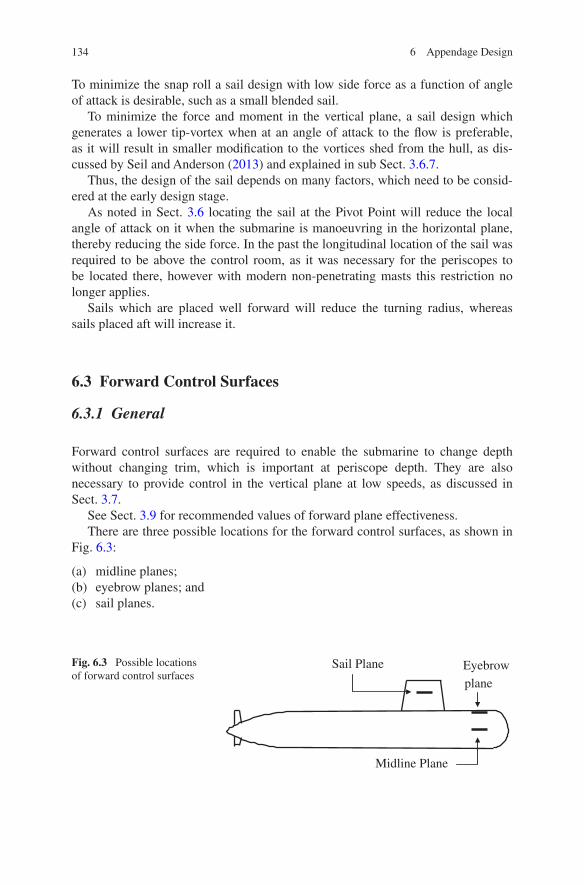
134 6 Appendage Design
To minimize the snap roll a sail design with low side force as a function of angle of attack is desirable, such as a small blended sail.
To minimize the force and moment in the vertical plane, a sail design which generates a lower tip-vortex when at an angle of attack to the flow is preferable, as it will result in smaller modification to the vortices shed from the hull, as dis-cussed by Seil and Anderson (2013) and explained in sub Sect. 3.6.7.
Thus, the design of the sail depends on many factors, which need to be consid-ered at the early design stage.
As noted in Sect. 3.6 locating the sail at the Pivot Point will reduce the local angle of attack on it when the submarine is manoeuvring in the horizontal plane, thereby reducing the side force. In the past the longitudinal location of the sail was required to be above the control room, as it was necessary for the periscopes to be located there, however with modern non-penetrating masts this restriction no longer applies.
Sails which are placed well forward will reduce the turning radius, whereas sails placed aft will increase it.
6.3 Forward Control Surfaces
6.3.1 General
Forward control surfaces are required to enable the submarine to change depth without changing trim, which is important at periscope depth. They are also necessary to provide control in the vertical plane at low speeds, as discussed in Sect. 3.7.
See Sect. 3.9 for recommended values of forward plane effectiveness.There are three possible locations for the forward control surfaces, as shown in
Fig. 6.3:
(a) midline planes;(b) eyebrow planes; and(c) sail planes.
Fig. 6.3 Possible locations of forward control surfaces
Sail Plane Eyebrow plane
Midline Plane

135
6.3.2 Midline Planes
Midline planes are in reasonably undisturbed flow, and the hull provides a posi-tive ground-board effect, thus increasing their effective aspect ratio, as shown in Fig. 6.4.
However, with midline planes the trailing-vortices may degrade the perfor-mance of sonar flank arrays, and they may be sucked into the propulsor, as shown in Fig. 6.5, increasing propulsor noise.
Midline planes need to be retractable. However, this also gives the opportunity to reduce resistance and noise associated with them, as the forward planes are not needed when operating deep and at high speed.
6.3.3 Eyebrow Planes
Eyebrow planes operate in the upward flow caused by the hull, as shown in Fig. 6.6. This means that unless the plane is twisted in the span-wise direction the angle of attack on the plane will be a function of the span-wise position. Thus, it will not be possible for the whole plane to be at zero angle of attack, and hence there will always be induced drag and associated tip-vortices. In addition, great care will be required with the root fillet and interaction with the hull as shown in Fig. 6.7. In most cases, there will be a gap when the plane is at a non-zero angle of attack, and this can result in vortices and associated noise.
Fig. 6.4 Cross section of midline plane
Fig. 6.5 Wake from midline plane
Wake from
forward plane
6.3 Forward Control Surfaces

136 6 Appendage Design
However, with the eyebrow plane the trailing-vortices are less likely to affect the flank arrays, and are less likely to be sucked into the propeller than with midline planes.
Eyebrow planes may or not need to be retractable, depending on their configuration.
6.3.4 Sail Planes
Sail planes are situated in reasonably undisturbed flow. The vortices from them won’t affect the flank arrays and are unlikely to be sucked into the propulsor, Fig. 6.8.
Sail planes will have a good ground-board effect, thus increasing their effective aspect ratio, as shown in Fig. 6.9. Sail planes do not need to be retractable, as they are contained completely inside the overall dimensions of the submarine.
Sail planes are generally located close to the Neutral Point (see Sect. 3.7). This means that by operating the sail planes alone it is possible to change the depth of the submarine without changing its trim. With earlier, manual, control systems this may have been useful, but with modern control techniques it is easy to apply a net vertical force at the Neutral Point from two well-spaced hydroplanes, making this feature less important. However, not having to operate the aft control surfaces when at periscope depth may be an advantage.
On the other hand, as they are not as far forward as either the midline, or the eye-brow planes, they have less lever arm to the Critical Point, making them less effec-tive when depth changes with trim are required. This also makes them less effective at low speeds, when submarine depth control relies on the forward planes.
Fig. 6.6 Eyebrow plane, showing upward flow due to the hull, and the wake from the plane
Wake from forward plane
Fig. 6.7 Cross section of eyebrow plane
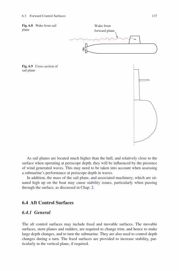
137
As sail planes are located much higher than the hull, and relatively close to the surface when operating at periscope depth, they will be influenced by the presence of wind generated waves. This may need to be taken into account when assessing a submarine’s performance at periscope depth in waves.
In addition, the mass of the sail plane, and associated machinery, which are sit-uated high up on the boat may cause stability issues, particularly when passing through the surface, as discussed in Chap. 2.
6.4 Aft Control Surfaces
6.4.1 General
The aft control surfaces may include fixed and movable surfaces. The movable surfaces, stern planes and rudders, are required to change trim, and hence to make large depth changes, and to turn the submarine. They are also used to control depth changes during a turn. The fixed surfaces are provided to increase stability, par-ticularly in the vertical plane, if required.
Fig. 6.8 Wake from sail plane
Wake from forward plane
Fig. 6.9 Cross section of sail plane
6.3 Forward Control Surfaces

138 6 Appendage Design
See Sect. 3.9 for recommended values of stern plane and rudder effectiveness.On an axisymmetric body with a single propulsor the aft control surfaces are
usually located forward of the propulsor. This means that they do not benefit from the increased flow from the propulsor, and that they cause wake distortions into the propulsor, increasing propulsor noise. Thus the number of aft control surfaces, and their interaction with the wake from the sail, need to be considered along with the propulsor blade number when considering their effect on acoustic signature. A propeller with the same number of blades as the number of wake regimes would generate significant acoustic noise, as each of the blades would be passing through a wake at the same time as discussed in sub Sect. 5.1.1. This should be avoided, as should any multiples of wake and propeller blade numbers. Note that if stators are fitted ahead of the propulsor then the wake from them also needs to be considered, as discussed in Sect. 5.2.
Ideally the aft control surfaces should be moved as far forward, and away from the propulsor, as possible. However, this will reduce the available span for the con-trol surfaces, due to the increase in tail cone diameter, and the need to avoid them protruding beyond the dimensions of the submarine, to avoid complications when coming alongside, as shown in Fig. 6.10.
It is important to note that as the submarine is symmetrical in the x-z plane, manoeuvres in the vertical plane only require a vertical force from the aft con-trol surfaces, whereas as it is not symmetrical in the x-y plane, manoeuvres in the horizontal plane will require both a force in the horizontal direction and one in the vertical direction to maintain constant depth as discussed in Sect. 3.6. Thus, when considering the size and configuration of the aft control surfaces this needs to be taken into account. There is little point in providing a large horizontal force capability if the vertical force available cannot maintain the depth when turning at maximum turn rate.
Aft hydroplanes must not extend beyond these lines
Fig. 6.10 U shape “bucket” defining limits of hydroplanes

139
6.4.2 Cruciform Configuration
The traditional arrangement for the aft control surfaces on submarines with a sin-gle axial propulsor is the cruciform configuration, as shown in Fig. 6.11. With this arrangement the vertical control surfaces (rudders) control the manoeuvring in the horizontal plane, and the horizontal control surfaces (stern planes) control the manoeuvring in the vertical plane. As the submarine is symmetrical in the x-z plane, manoeuvres in the vertical plane only require operation of the stern planes, whereas as it is not symmetrical in the x-y plane, manoeuvres in the horizontal plane will require operation of the rudders, together with operation of the stern planes (and bow planes) to maintain constant depth.
As discussed in Sect. 3.1 it is normally desirable for a submarine to have a high degree of stability in the vertical plane, and a high degree of manoeuvrabil-ity (lower stability) in the horizontal plane. The cruciform arrangement makes it possible to achieve this. For example, it is possible to have a fixed fin with a flap for the stern planes, and an all moving arrangement for the rudders, as shown in Fig. 6.11a. Note that this is not essential, and many submarines have a fixed fin and flap for the rudder, as well as for the horizontal plane.
With the cruciform configuration the lower rudder is often smaller, and with a lower aspect ratio, than desirable, as it is not permitted for it to extend below the keel of the submarine. This may make manoeuvring on the surface difficult. On the other hand, the upper rudder may be made larger, which will also help reduce
(a)
(b)
Fig. 6.11 Cruciform configuration for aft planes. a Schematic. b View from astern
6.4 Aft Control Surfaces

140 6 Appendage Design
the snap roll when submerged, but as the upper rudder operates in the wake from the sail it will be less effective.
The span of the horizontal planes is also limited by the requirement for them not to protrude beyond the beam of the submarine as shown in Fig. 6.10.
A major disadvantage of the cruciform configuration exists when the two stern planes are connected to each other, and the two rudders are connected to each other. This is often done to reduce mechanical complexity. Thus, if there is a jam in the stern planes, for example, this cannot be recovered by moving the other stern plane. See Sect. 3.10 for a discussion of Manoeuvring Limitation Diagrams. If the control surfaces can be moved independently of each other, then this limita-tion would be significantly reduced.
6.4.3 X-Form Configuration
An alternative arrangement for the aft control surfaces is the X-form configuration, as shown in Figs. 6.12 and 6.13. With this configuration, as each control surface is identical, it is not so easy to meet the generally accepted requirement of good stability in the vertical plane and good manoeuvring in the horizontal plane. The need for good stability in the vertical plane may be less important for low speed conventional submarines (SSKs) than for the higher speed nuclear powered sub-marines (SSNs), however this aspect does need to be considered with the X-plane configuration.
It may be possible to go some way towards the requirement for different degrees of stability in the vertical and horizontal planes by not positioning the individual control surfaces at an angle of 90° to each other, and/or adding a hori-zontal fixed stabilizer.
One advantage of the X-form configuration is that each of the control surfaces can have a much longer span than with the cruciform configuration before they
Fig. 6.12 X-form configuration for aft planes (courtesy of DSTO)
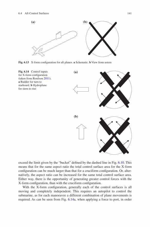
141
exceed the limit given by the “bucket” defined by the dashed line in Fig. 6.10. This means that for the same aspect ratio the total control surface area for the X-form configuration can be much larger than that for a cruciform configuration. Or, alter-natively, the aspect ratio can be increased for the same total control surface area. Either way, there is the opportunity of generating greater control forces with the X-form configuration, than with the cruciform configuration.
With the X-form configuration, generally each of the control surfaces is all moving and completely independent. This requires an autopilot to control the submarine, as for each manoeuvre a different combination of plane movements is required. As can be seen from Fig. 6.14a, when applying a force to port, in order
(a) (b)
Fig. 6.13 X-form configuration for aft planes. a Schematic. b View from astern
Fig. 6.14 Control inputs for X-form configuration (taken from Renilson 2011). a Rudder for turn to starboard. b Hydroplane for stern to rise
(a)
(b)
6.4 Aft Control Surfaces

142 6 Appendage Design
to turn to starboard, each control surface is required to operate. Vertical upwards forces are generated which are cancelled out by vertical downwards forces. Hence, to create a given effective force considerably greater total force is generated for the X-form configuration than for the cruciform configuration. The same can be seen in Fig. 6.14b when creating a vertical force (Renilson 2011).
Thus, a greater total force will be required for the X-plane configuration. This will result in greater formation of vortices which will impinge on the propulsor, and on greater induced drag which will result in more power being required to maintain a given speed than for the equivalent cruciform configuration.
However, as most submarines are not symmetrical about the x-y plane, when turning a vertical force is often required to maintain depth. With the cruciform arrangement this means that for a level turn the aft hydroplanes are used in addition to the rudder. However, for the X-form configuration each individual hydroplane already provides a vertical force, so, depending on the level of asymmetry, the total force may not be greater for the X-form configuration, as illustrated in Fig. 6.15. Whether the total force is greater for the cruciform or the X-form for a particular manoeuvre will depend on the degree of asymmetry that the submarine has.
As a submarine requires a vertical force when turning to compensate for the asymmetry, this may be an effective limit to the rate of turn, not the magnitude of the horizontal force. For example, with the X-form configuration adopted by Crossland et al. (2011, 2012) the maximum effective rudder angle is about 25°, with greater angles not being possible.
For an X-form configuration the forces and moments generated by each indi-vidual plane need to be considered in the representations of the hydrodynamic
Fig. 6.15 Comparison of control inputs for a cruciform and X-form configurations when turning a submarine which is not symmetrical about the x-y plane (taken from Renilson 2011). a Cruciform configuration. b X-form configuration
(a)
(b)
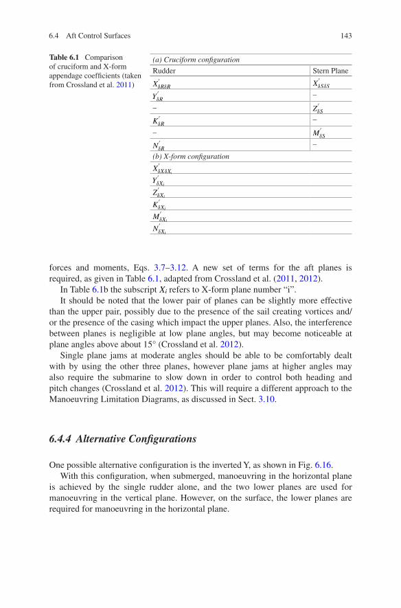
143
forces and moments, Eqs. 3.7–3.12. A new set of terms for the aft planes is required, as given in Table 6.1, adapted from Crossland et al. (2011, 2012).
In Table 6.1b the subscript Xi refers to X-form plane number “i”.It should be noted that the lower pair of planes can be slightly more effective
than the upper pair, possibly due to the presence of the sail creating vortices and/or the presence of the casing which impact the upper planes. Also, the interference between planes is negligible at low plane angles, but may become noticeable at plane angles above about 15° (Crossland et al. 2012).
Single plane jams at moderate angles should be able to be comfortably dealt with by using the other three planes, however plane jams at higher angles may also require the submarine to slow down in order to control both heading and pitch changes (Crossland et al. 2012). This will require a different approach to the Manoeuvring Limitation Diagrams, as discussed in Sect. 3.10.
6.4.4 Alternative Configurations
One possible alternative configuration is the inverted Y, as shown in Fig. 6.16.With this configuration, when submerged, manoeuvring in the horizontal plane
is achieved by the single rudder alone, and the two lower planes are used for manoeuvring in the vertical plane. However, on the surface, the lower planes are required for manoeuvring in the horizontal plane.
Table 6.1 Comparison of cruciform and X-form appendage coefficients (taken from Crossland et al. 2011)
(a) Cruciform configuration
Rudder Stern Plane
X′δRδR
X′δSδS
Y′δR
–
– Z′δS
K′δR
–
– M′δS
N′δR
–
(b) X-form configuration
X′δXδXi
Y′δXi
Z′δXi
K′δXi
M′δXi
N′δXi
6.4 Aft Control Surfaces
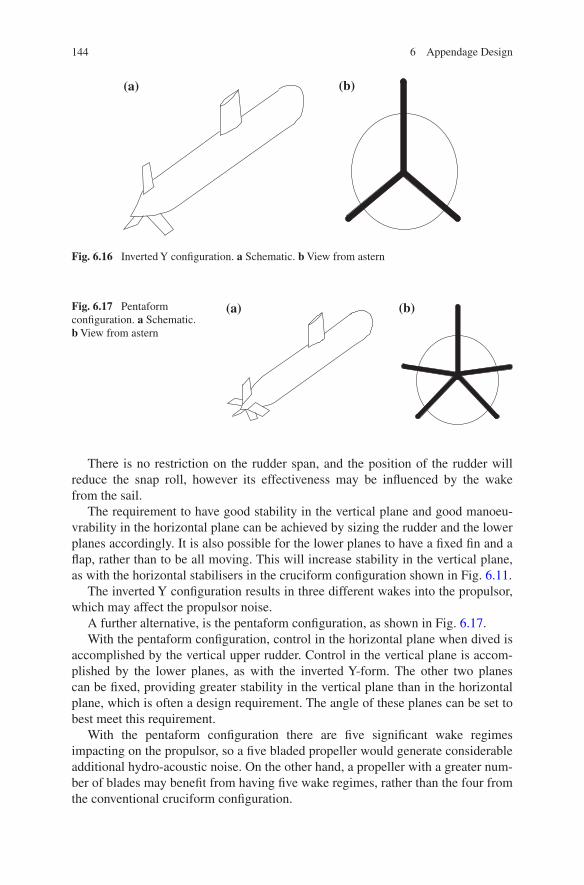
144 6 Appendage Design
There is no restriction on the rudder span, and the position of the rudder will reduce the snap roll, however its effectiveness may be influenced by the wake from the sail.
The requirement to have good stability in the vertical plane and good manoeu-vrability in the horizontal plane can be achieved by sizing the rudder and the lower planes accordingly. It is also possible for the lower planes to have a fixed fin and a flap, rather than to be all moving. This will increase stability in the vertical plane, as with the horizontal stabilisers in the cruciform configuration shown in Fig. 6.11.
The inverted Y configuration results in three different wakes into the propulsor, which may affect the propulsor noise.
A further alternative, is the pentaform configuration, as shown in Fig. 6.17.With the pentaform configuration, control in the horizontal plane when dived is
accomplished by the vertical upper rudder. Control in the vertical plane is accom-plished by the lower planes, as with the inverted Y-form. The other two planes can be fixed, providing greater stability in the vertical plane than in the horizontal plane, which is often a design requirement. The angle of these planes can be set to best meet this requirement.
With the pentaform configuration there are five significant wake regimes impacting on the propulsor, so a five bladed propeller would generate considerable additional hydro-acoustic noise. On the other hand, a propeller with a greater num-ber of blades may benefit from having five wake regimes, rather than the four from the conventional cruciform configuration.
(a) (b)
Fig. 6.16 Inverted Y configuration. a Schematic. b View from astern
Fig. 6.17 Pentaform configuration. a Schematic. b View from astern
(a) (b)

145
Finally, as noted in sub Sect. 6.4.3, horizontal stabilizers can be added to the X-form configuration, resulting in six appendages. This will result in six signifi-cant wake regimes impacting on the propulsor.
References
Crossland P, Kimber NI, Thompson N (2012) Understanding the manoeuvring performance of an X-plane submarine in deep water and near the free surface. In: Pacific 2012: international maritime conference, Sydney, Jan 2012
Crossland P, Marchant P, Thompson N (2011) Evaluating the manoeuvring performance of an X-Plane submarine. In: Proceedings of warship 2011: naval submarines and UUVs, Royal Institution of Naval Architects, Bath, 29–30 June 2011
Kormilitsin YN, Khalizev OA (2001) Theory of submarine design. Saint Petersburg State Maritime Technical University, Russia
Renilson MR (2011) Submarine manoeuvring and appendage design—what is the best option for a large SSK? In: Proceedings of the submarine institute of Australia technology conference 2011, Science technology and engineering, Adelaide, 8–10 Nov 2011
Seil GJ, Anderson B (2012) A comparison of submarine fin geometry on the performance of a generic submarine. In: Proceedings of Pacific 2012 international maritime conference, Sydney, 2012
Seil G, Anderson B (2013) The influence of submarine fin design on heave force and pitching moment in steady drift. In: Pacific 2013: international maritime conference, Sydney, Oct 2013
6.4 Aft Control Surfaces
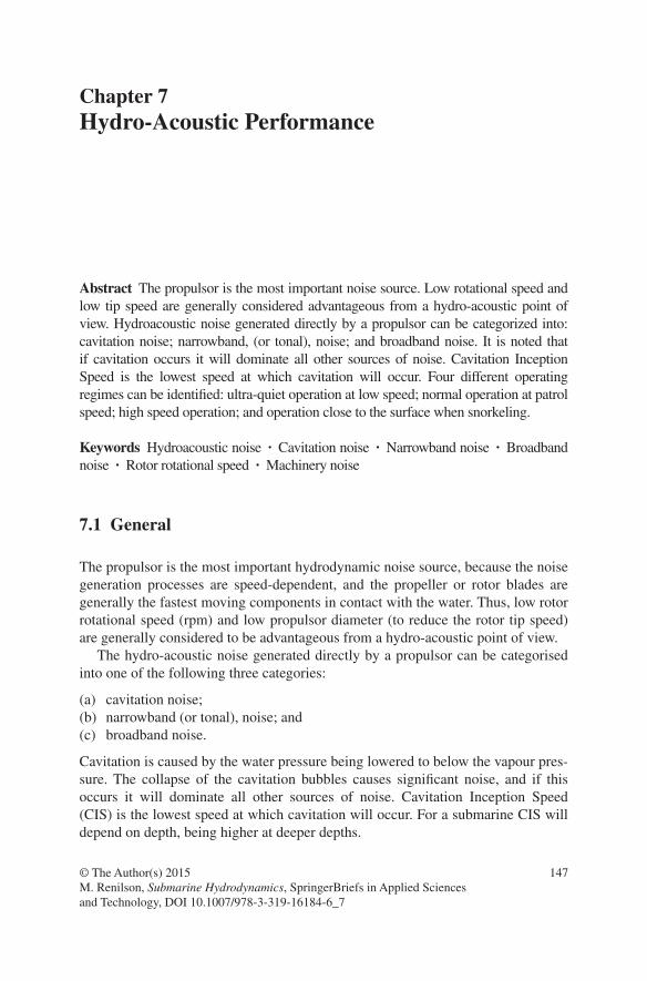
147
Abstract The propulsor is the most important noise source. Low rotational speed and low tip speed are generally considered advantageous from a hydro-acoustic point of view. Hydroacoustic noise generated directly by a propulsor can be categorized into: cavitation noise; narrowband, (or tonal), noise; and broadband noise. It is noted that if cavitation occurs it will dominate all other sources of noise. Cavitation Inception Speed is the lowest speed at which cavitation will occur. Four different operating regimes can be identified: ultra-quiet operation at low speed; normal operation at patrol speed; high speed operation; and operation close to the surface when snorkeling.
Keywords Hydroacoustic noise · Cavitation noise · Narrowband noise · Broadband noise · Rotor rotational speed · Machinery noise
7.1 General
The propulsor is the most important hydrodynamic noise source, because the noise generation processes are speed-dependent, and the propeller or rotor blades are generally the fastest moving components in contact with the water. Thus, low rotor rotational speed (rpm) and low propulsor diameter (to reduce the rotor tip speed) are generally considered to be advantageous from a hydro-acoustic point of view.
The hydro-acoustic noise generated directly by a propulsor can be categorised into one of the following three categories:
(a) cavitation noise;(b) narrowband (or tonal), noise; and(c) broadband noise.
Cavitation is caused by the water pressure being lowered to below the vapour pres-sure. The collapse of the cavitation bubbles causes significant noise, and if this occurs it will dominate all other sources of noise. Cavitation Inception Speed (CIS) is the lowest speed at which cavitation will occur. For a submarine CIS will depend on depth, being higher at deeper depths.
Chapter 7Hydro-Acoustic Performance
© The Author(s) 2015 M. Renilson, Submarine Hydrodynamics, SpringerBriefs in Applied Sciences and Technology, DOI 10.1007/978-3-319-16184-6_7

148 7 Hydro-Acoustic Performance
Generally, submarine propulsors are designed to avoid cavitation, which is possible for deeply submerged submarines due to the additional head of water above the propulsor. However, cavitation may occur when the submarine is oper-ating close to the surface, and/or in an “off-design” condition, such as when manoeuvring.
In general, cavitation margins are defined by inception of (Anderson et al. 2009):
(a) suction-side cavitation;(b) suction-side tip-vortex cavitation;(c) pressure-side cavitation;(d) pressure-side tip-vortex cavitation; and(e) hub-vortex cavitation.
Strategies to ensure that each of these cavitation mechanisms is avoided are adopted in the design of a submarine propeller. These include: ensuring adequate blade area; thicker blades; and reducing the loading at the blade tip and the hub. In addition, the tip speed is reduced if possible, and the gap between the rotor tip and the duct in a pumpjet minimised.
Narrowband noise occurs at the blade passing rate, and at harmonics of this. It is caused by the blades passing through the non-uniform wake generated by the hull and appendages ahead of the propulsor. Therefore the design of the hull and appendages ahead of the propulsor has a dominating influence on the character-istics of the narrowband noise generated by the propulsor. As noted in Chap. 5, the number of rotor blades is usually a prime number to reduce the effect of harmonics.
Broadband noise is generated by direct turbulent interactions, and it cannot be predicted by the use of existing numerical techniques because the relevant pro-cesses are represented by approximate forms, rather than modelled in their own right. Broadband noise is generated by turbulent fluctuations of the boundary layer on the blade, and is more directly associated with flow turbulence than narrow-band noise.
In addition to noise generated directly by the propulsor, the fluctuating forces on the propulsor can set up resonances in the submarine, which in turn can gener-ate radiated acoustic noise.
Low frequency noise travels further than high frequency noise. Thus, for sub-marine detection low frequency noise is far more critical.
At low speed very little hydrodynamic noise is produced. Machine noise may dominate, and cavitation is very unlikely. At intermediate speeds hydrodynamic flow noise will be important, both broadband and narrowband. At high speeds, particularly when running close to the surface, cavitation may occur, and when it does this dominates all noise sources.
Thus, it is clear that the relative importance of the various noise sources differs depending on the speed and operating depth of the submarine. However, detailed information about this is highly classified and not generally available in the public domain.

149
Four different operating regimes can be identified:
(a) ultra-quiet operation at low speed;(b) normal operation at patrol speed;(c) high speed operation; and(d) operation close to the surface when snorkelling.
(a) Ultra-Quiet Operation at Low SpeedIn the ultra-quiet mode a submarine will be travelling below about four knots. At this speed hydrodynamic noise is minimal, and machinery noise will normally be the most important noise source (Miasnikov 1995).(b) Normal Operation at Patrol SpeedAt speeds between about eight knots and fifteen knots the hydrodynamic flow noise will dominate. For well-designed deeply submerged submarines cavitation should not be an issue. Hence, the broadband and narrowband noise generated by the propulsor are the important issues for this speed range.(c) High Speed OperationAs hydrodynamic flow noise is proportional to speed raised to the sixth power, above about fifteen knots hydrodynamic noise from the propulsor becomes very significant. Submarines operating at these speeds will be significantly more noisy than those operating at speeds below this, with the hydrodynamic noise from the propulsor being critical (Miasnikov 1995).
At these higher speeds, the fluctuating forces from the propulsor can hit hull struc-tural modes, which may cause increased radiated acoustic noise from the submarine. An example of this is the first ‘accordion mode’, where the stern and the bow vibrate. This is far less likely to be an issue at speeds below around fifteen knots.
For a deeply submerged submarine cavitation should not be an issue until speeds of the order of twenty to twenty five knots. Above this speed, cavitation noise may dominate (Miasnikov 1995).
In addition, at speeds above about fifteen knots the hydrodynamic noise on the hull is also an issue, which may make it difficult to operate hull borne sonar.(d) Operation Close to the Surface when SnorkellingWhen an SSK is snorkelling it will generate increased machinery noise. Also it is possible that cavitation will occur due to: the reduction in static head; the increase in drag due to the presence of the free surface and the drag on the masts resulting in increased thrust required; and the activation of the hydroplanes to control the boat close to the surface, particularly in waves.
Hydrodynamic flow noise is unlikely to be an important issue in this operating regime.
As the critical noise source depends on the operating regime, the mitigation pro-cesses to reduce noise for a particular submarine will depend on which regimes it operates in. For example, SSKs are generally not able to operate at speeds greater than about fifteen knots, so measures to reduce noise for submarines operating in the high speed regime are not applicable. Equally, SSNs are not required to snorkel close to the surface, so measures to reduce noise for submarines operating in this regime may not be applicable to them.
7.1 General

150 7 Hydro-Acoustic Performance
References
Andersen P, Kappel JJ, Spangenberg E (2009) Aspects of propeller developments for a subma-rine. In: First international symposium on marine propulsors, Trondheim, Norway, 2009
Miasnikov EV (1995) The future of Russia’s strategic nuclear forces, discussions and arguments. Centre for Arms Control, Energy and Environmental Studies, Moscow Institute of Physics and Technology, Russia


