Page 1
MASS DIFFUSION AND CHEMICAL KINETIC DATA FOR
JET FUEL SURROGATES
by
Kyungchan Chae
A dissertation submitted in partial fulfillment of the requirements for the degree of
Doctor of Philosophy (Mechanical Engineering)
in the University of Michigan 2010
Doctoral Committee:
Associate Professor Angela Violi, Chair Professor Margaret S. Wooldridge Associate Professor Hong G. Im Associate Professor Christian M. Lastoskie Research Fellow Paolo Elvati
Page 2
Success is a journey not a destination.
The way you react to change will greatly affect your trip.
Erik Olesen
One who fears failure limits its activities.
Failure is only the opportunity to begin again more intelligently.
Henry Ford
Page 3
© Kyungchan Chae
2010
Page 4
ii
Acknowledgements
First of all, I would like to express my deepest appreciation to Professor Angela Violi
for giving me a wonderful chance to work on new scientific research and for the
knowledgeable advice.
I also would like to thank my doctoral committee members, Professor Margaret S.
Wooldridge, Professor Hong G. Im, Professor Christian M. Lastoskie and Dr. Paolo
Elvati.
The advice from Dr. Elvati on my thesis was invaluable. I am really grateful for his
help.
The help from all former and current group members, Dr. Steve Fiedler, Dr. Seungho
Choi, Dr. Lam Huynh, Dr. Wendung Hsu, Dr. Hairong Tao, Dr. Soumik Banerjee,
Seung-hyun Chung, Kuang-chuan Lin, Jason Lai, Adaleena Mookerjee, was
indispensable.
All of my family members gave me their love and support.
Most of all, I would like to express my greatest appreciation to my wife, Soojin Kim.
This dissertation would not have been possible without her support and patience.
Finally, I would like to thank Dr. Julian M. Tishkoff and U. S. Air Force Office of
Scientific Research for their support and grant for this research.
Page 5
iii
Table of Contents
Acknowledgements ii
List of Figures vii
List of Tables xiv
List of Appendices xv
Abstract xvi
Chapter 1
1. Introduction 1
1.1 Fuel surrogates 1
1.2 Mass diffusion 4
1.2.1 The effect of mass diffusion on flame modeling 5
1.2.2 Approach for diffusion of polyatomic molecules 7
1.3 Kinetic mechanisms 8
1.4 Outline 10
2. Mutual diffusion coefficients of hydrocarbons in nitrogen 13
2.1 Investigation of mass diffusion 13
2.1.1 Gas kinetic theory 13
Page 6
iv
2.1.2 Green-Kubo formula and MD simulations 17
2.2 Computational method: Molecular Dynamics simulations 19
2.2.1 All-atom Force field 19
2.2.2 Potential model 21
2.2.3 Simulation method 23
2.2.4 The effect of the thermostat 23
2.2.5 Velocity correlation 26
2.3 Benchmark of computational approaches 27
2.3.1 The effect of system size 27
2.3.2 The effect of concentration 28
2.3.3 Validity of atomistic force field for high temperature gas mixture 29
2.4 Diffusion coefficients of heptane isomers 31
2.4.1 Configurations of heptane isomers 31
2.4.2 Simulation results 32
2.5 Diffusion coefficients of hydrocarbon molecules 39
2.5.1 Linear alkanes 40
2.5.2 Cycloalkanes 44
2.5.3 Aromatic molecules 48
2.6 Comparison with gas kinetic theory 56
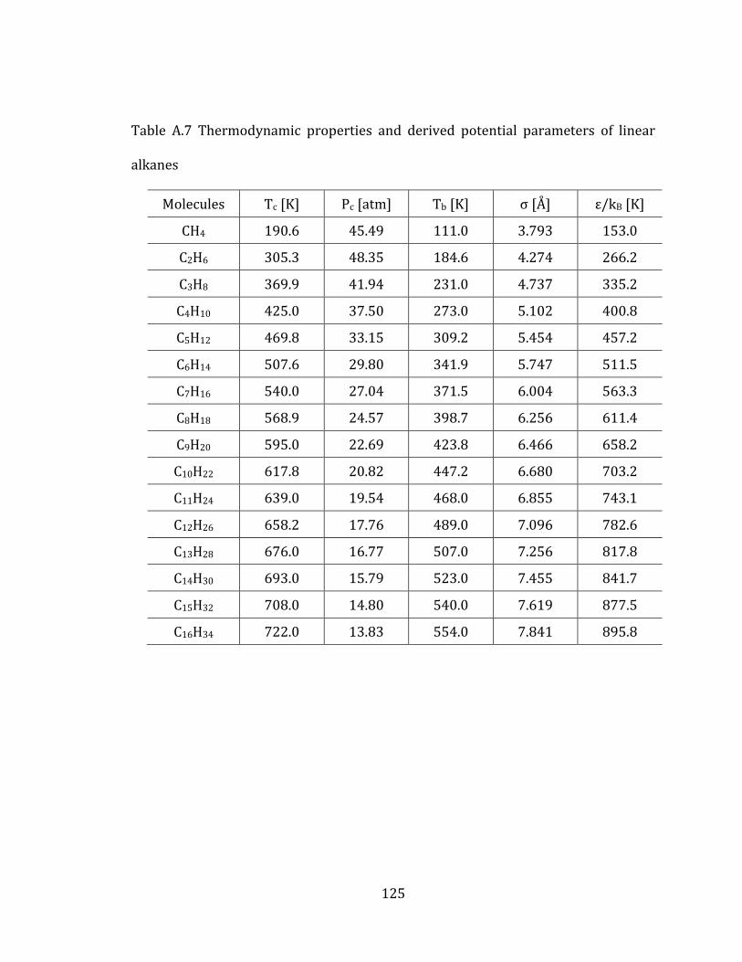
2.6.1 Thermodynamic properties and potential parameters 57
Page 7
v
2.6.2 Linear alkanes 57
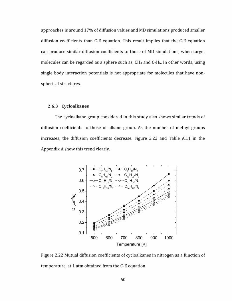
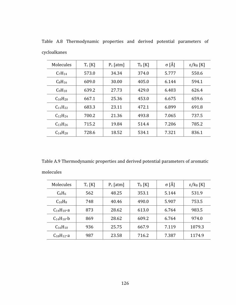
2.6.3 Cycloalkanes 60
2.6.4 Aromatic molecules 61
2.7 The effect of molecular configurations 63
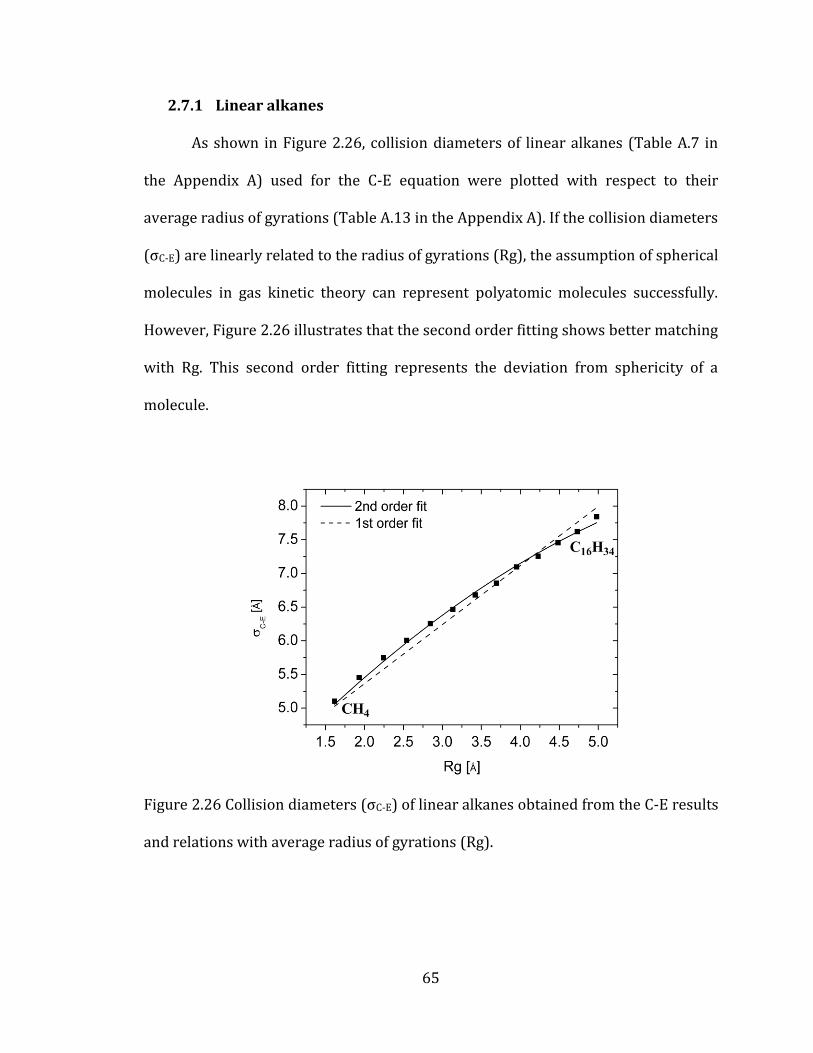
2.7.1 Linear alkanes 65
2.7.2 Cycloalkanes 68
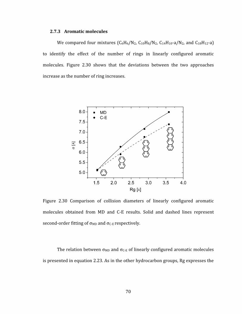
2.7.3 Aromatic molecules 70
2.8 Conclusions 72
3. The equivalent single body potentials of polyatomic molecules 74
3.1 The effect of potentials on diffusion 74
3.2 Thermodynamic properties from MD simulations 75
3.2.1 Chemical potentials 76
3.2.2 Simulation method 79
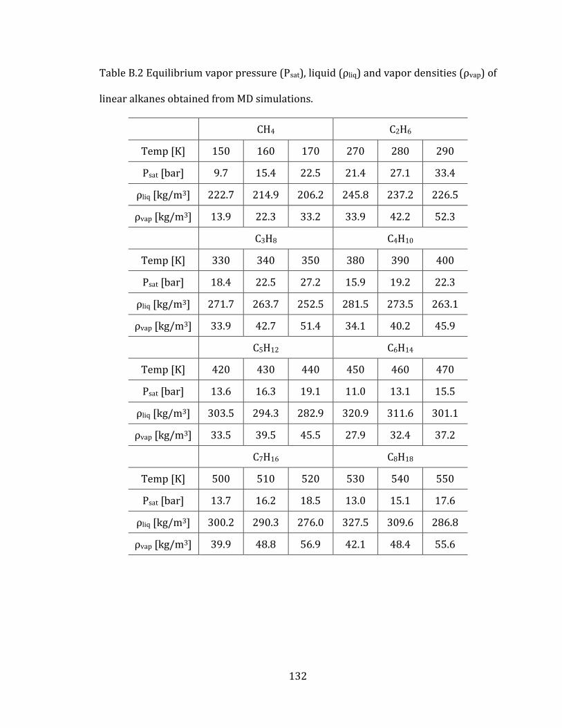
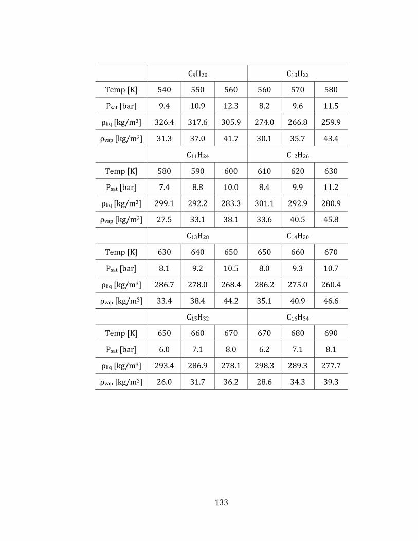
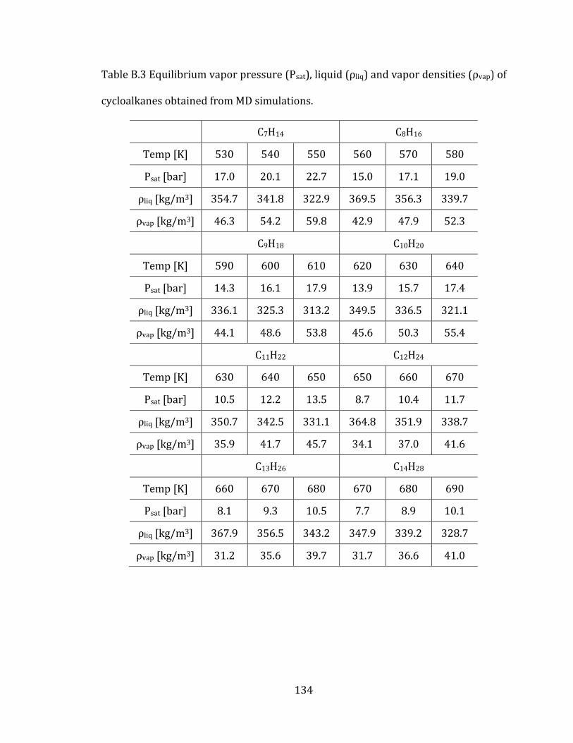
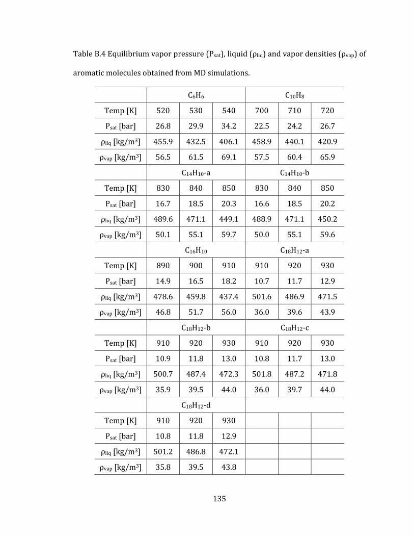
3.2.3 Equilibrium vapor pressure and densities 82
3.2.4 Computed thermodynamic properties 85
3.3 Equivalent single body potentials of all atom potentials 86
3.4 Comparison with the C-E equation and MD simulations 87
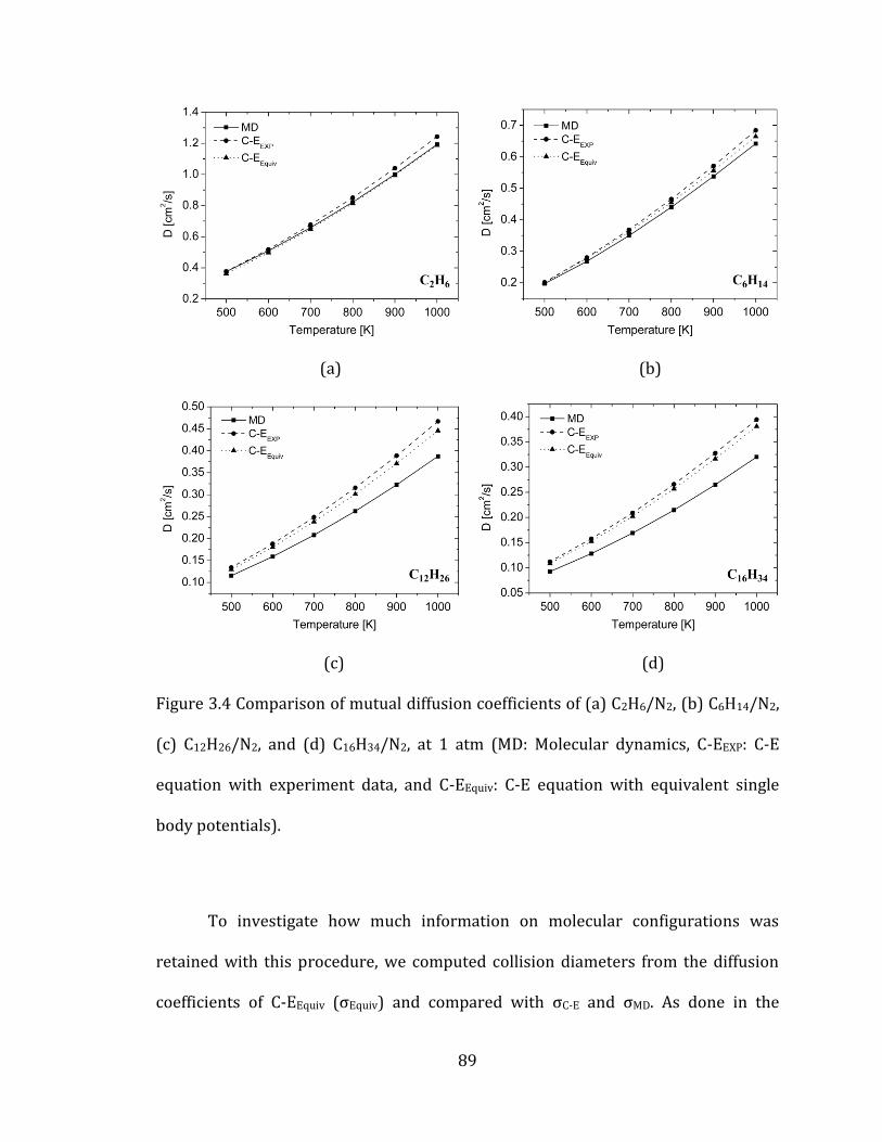
3.4.1 Linear alkanes 87
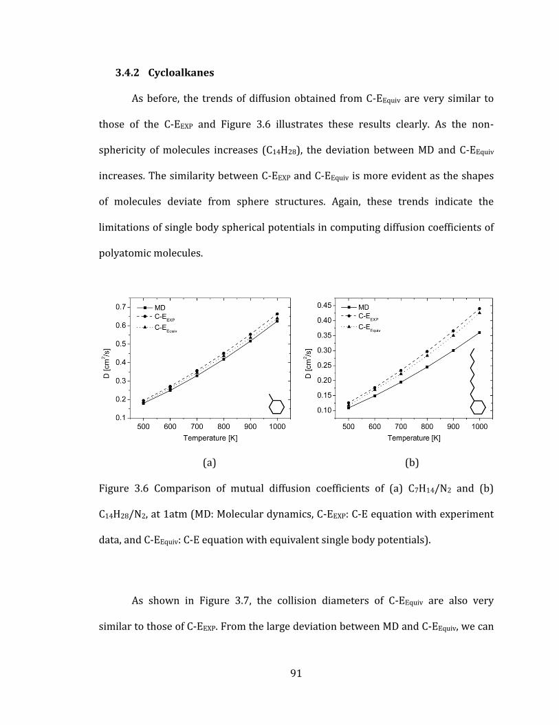
3.4.2 Cycloalkanes 91
3.4.3 Aromatic molecules 92
Page 8
vi
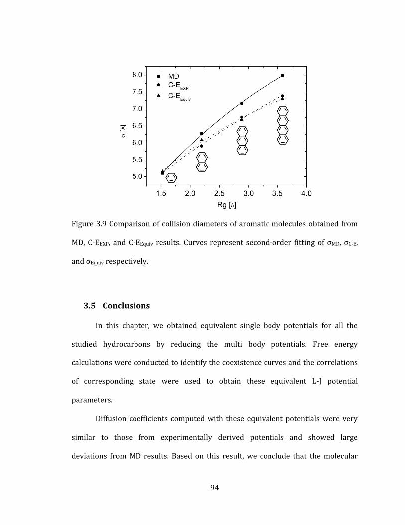
3.5 Conclusions 94
4. Breakdown mechanisms of Decalin 96
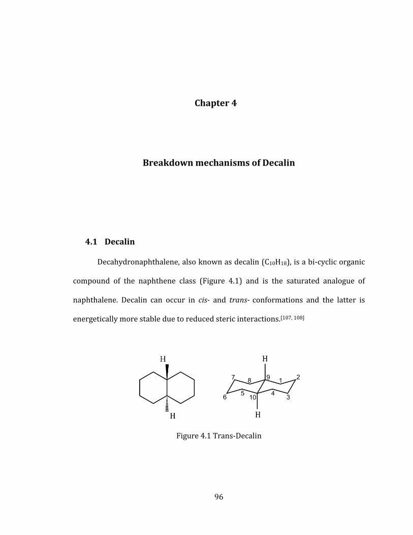
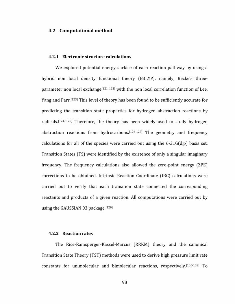
4.1 Decalin 96
4.2 Computational method 98
4.2.1 Electronic structure calculations 98
4.2.2 Reaction rates 98
4.3 Reaction pathways 100
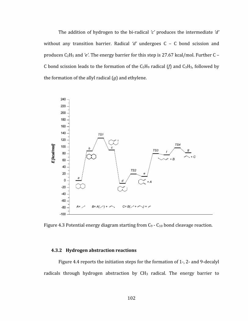
4.3.1 Carbon – carbon bond cleavage reactions 101
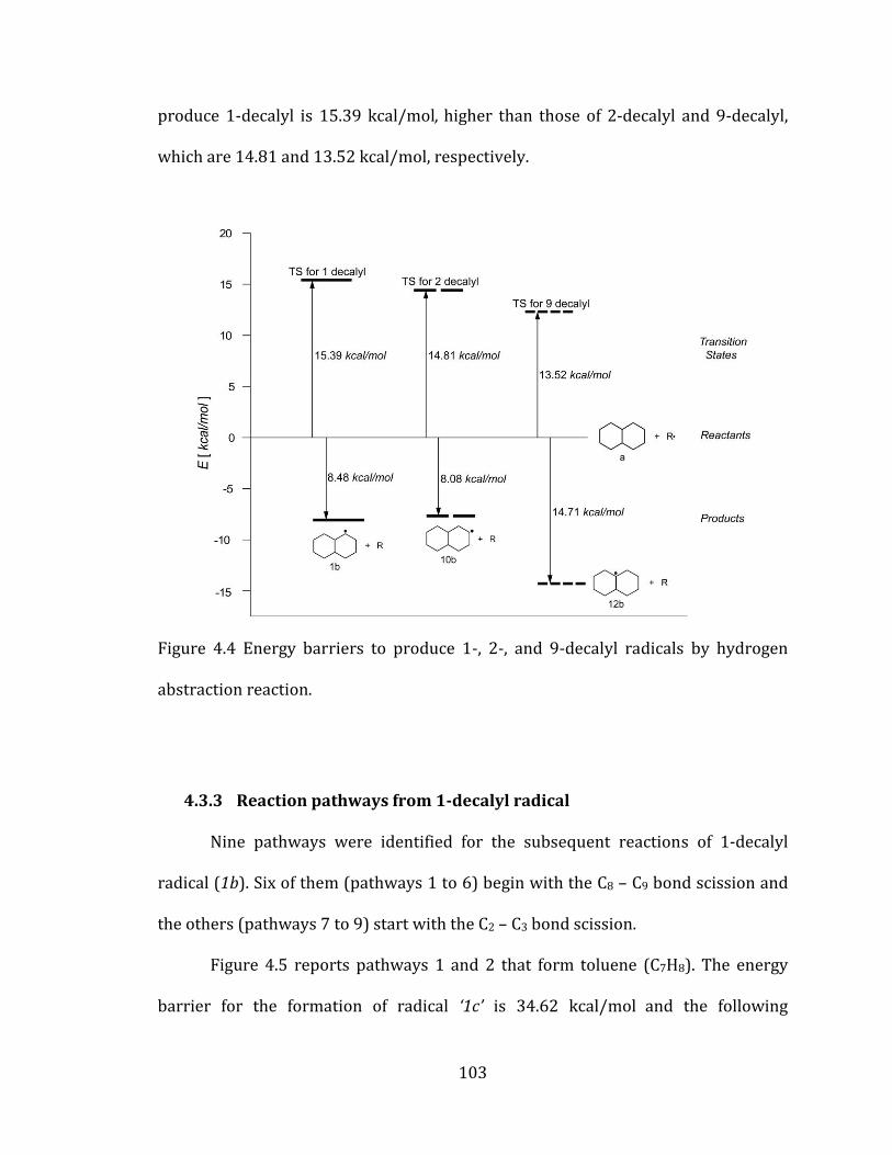
4.3.2 Hydrogen abstraction reactions 102
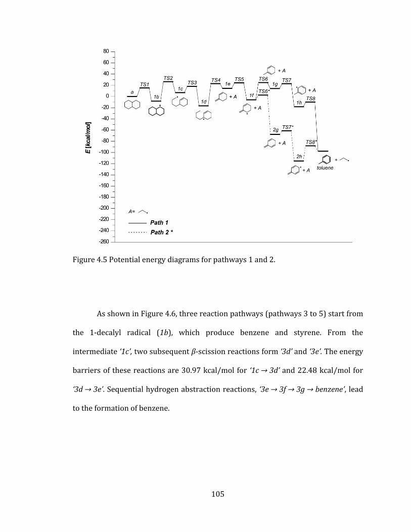
4.3.3 Reaction pathways from 1-decalyl radical 103
4.3.4 Reaction pathways from 2-decalyl radical 110
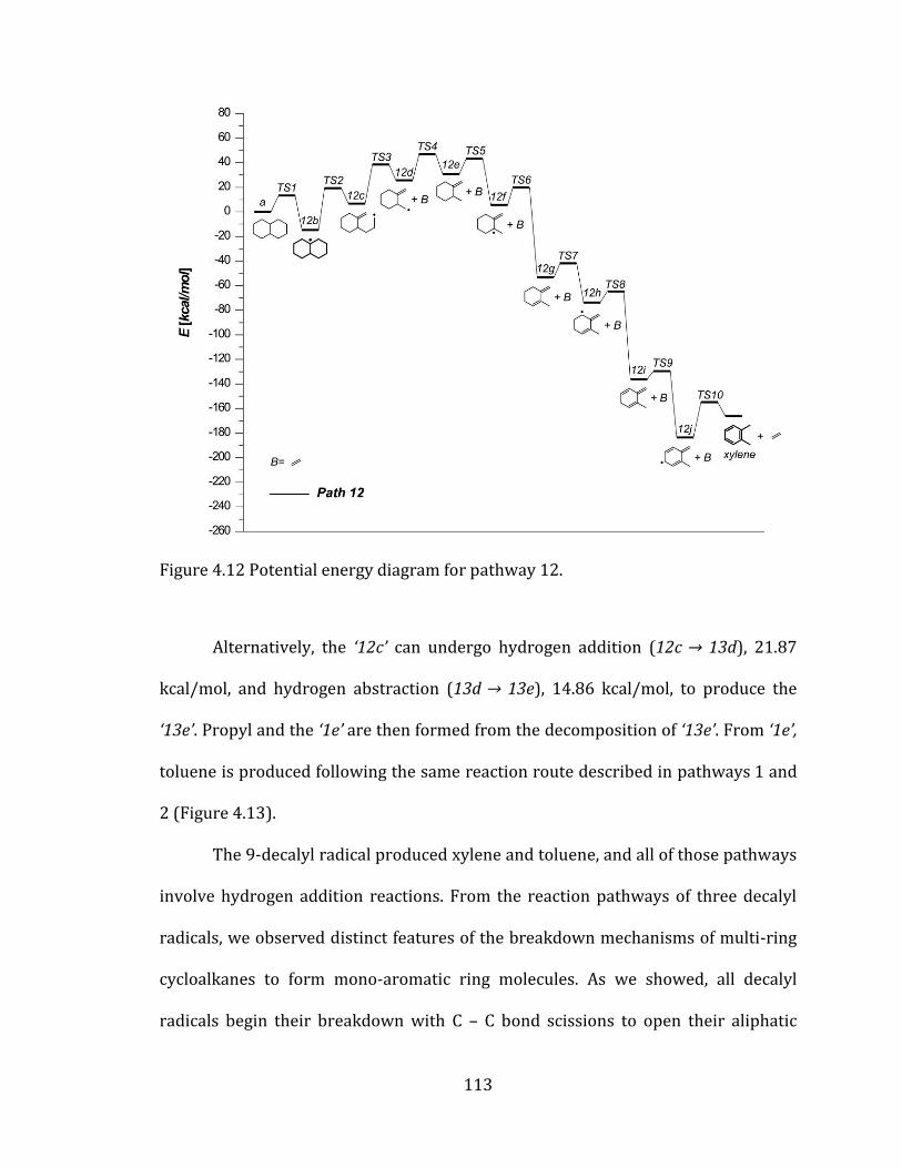
4.3.5 Reaction pathways from 9-decalyl radical 112
4.4 Kinetic modeling 115
4.5 Conclusions 117
5. Conclusions 118
Appendices 122
References 152
Page 9
vii
List of Figures
Figure 2.1 Comparison of velocity auto-correlation functions of n-C7H16 with NVE
and NVT ensembles with 1.0 ps coupling parameter at 1 atm and (a) 500K, (b)
1000K. ...................................................................................................................................................... 25
Figure 2.2 Normalized velocity correlation functions of n-C7H16 in the mixture at 1
atm and (a) 500K, (b) 1000K. ......................................................................................................... 26
Figure 2.3 Mutual diffusion coefficients of n-C7H16/N2 mixtures at 1 atm for
different system sizes with error bars obtained from MD simulations. ......................... 27
Figure 2.4 Mutual diffusion coefficients of n-C3H8/N2 and n-C4H10/N2 mixture at 1
atm (MD: Molecular Dynamics simulations, EXP: experiment). ........................................ 30
Figure 2.5 Molecular configurations of the six heptane isomers. .................................... 32
Figure 2.6 Radial distribution functions of n-C7H16/N2 mixture at 500K, 1 atm. ...... 33
Figure 2.7 Mutual diffusion coefficients of heptane isomers in nitrogen with error
bars at two different temperatures and 1 atm: Isomers – (1: n-C7H16, 2: 2-C7H16, 3:
2,2-C7H16, 4: 2,3-C7H16, 5: 3,3-C7H16, 6: 2,2,3-C7H16) .............................................................. 35
Page 10
viii
Figure 2.8 Mutual diffusion coefficients of heptane isomers in nitrogen versus the
square inverse of radius of gyrations (Rg) of the isomers at 1 atm and (a) 500K and
(b) 1000K. ............................................................................................................................................... 37
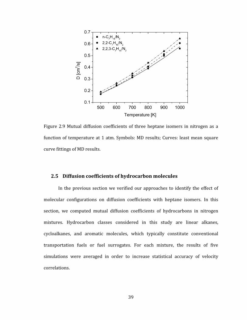
Figure 2.9 Mutual diffusion coefficients of three heptane isomers in nitrogen as a
function of temperature at 1 atm. Symbols: MD results; Curves: least mean square
curve fittings of MD results. ............................................................................................................. 39
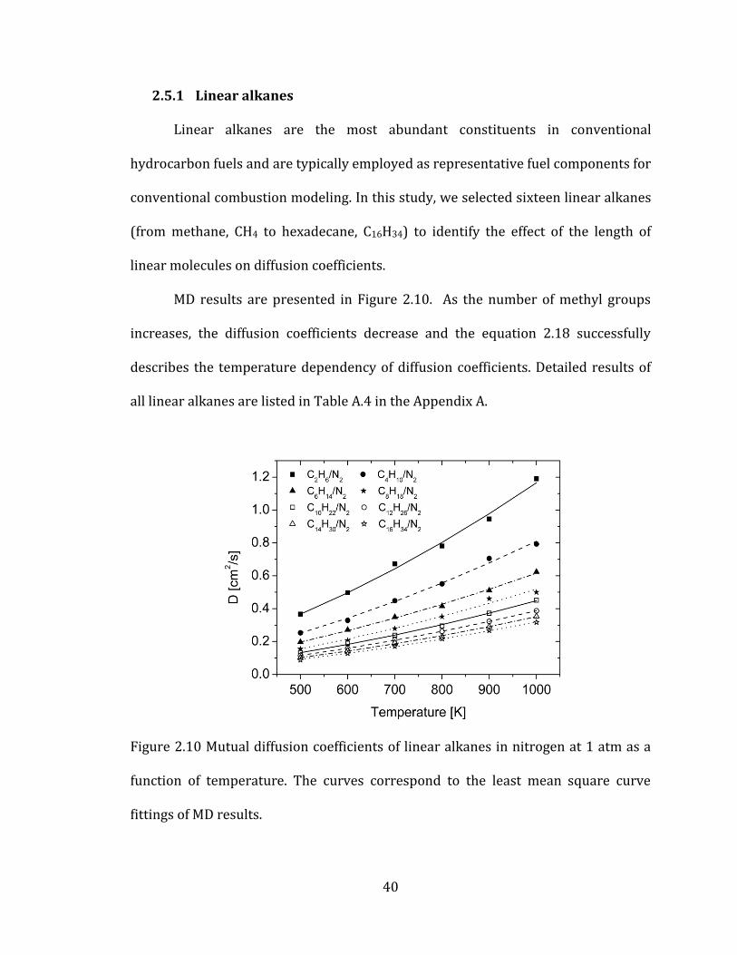
Figure 2.10 Mutual diffusion coefficients of linear alkanes in nitrogen at 1 atm as a
function of temperature. The curves correspond to the least mean square curve
fittings of MD results. ......................................................................................................................... 40
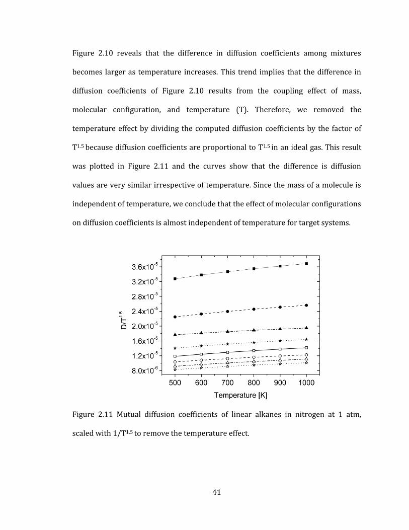
Figure 2.11 Mutual diffusion coefficients of linear alkanes in nitrogen at 1 atm,
scaled with 1/T1.5 to remove the temperature effect. ............................................................ 41
Figure 2.12 Self diffusion coefficients of (a) linear alkanes and (b) nitrogen in the
mixtures, at 1atm. The curves correspond to the least mean square curve fittings of
MD results. .............................................................................................................................................. 43
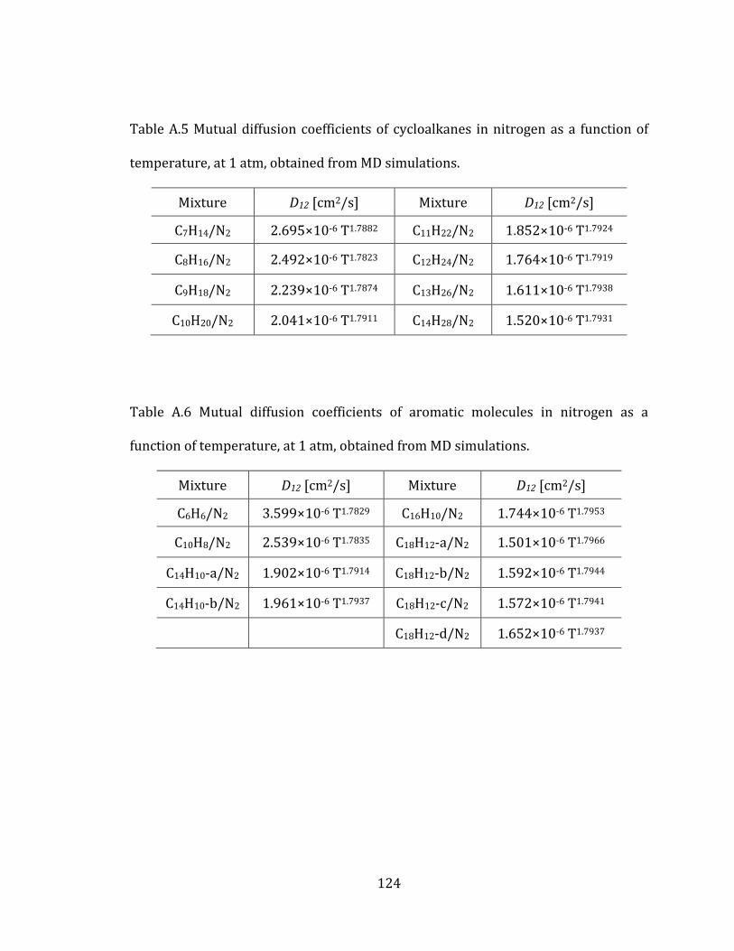
Figure 2.13 Mutual diffusion coefficients of cycloalkanes in nitrogen as a function of
temperature, at 1 atm. ....................................................................................................................... 45
Figure 2.14 Self diffusion coefficients of (a) cycloalkanes and (b) nitrogen in the
mixtures, at 1 atm. The curves correspond to the least square curve fittings of MD
results. ...................................................................................................................................................... 46
Page 11
ix
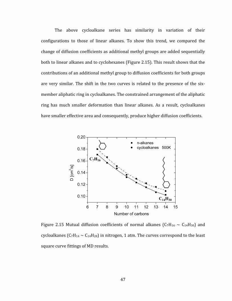
Figure 2.15 Mutual diffusion coefficients of normal alkanes (C7H16 ~ C14H30) and
cycloalkanes (C7H14 ~ C14H28) in nitrogen, 1 atm. The curves correspond to the least
square curve fittings of MD results. .............................................................................................. 47
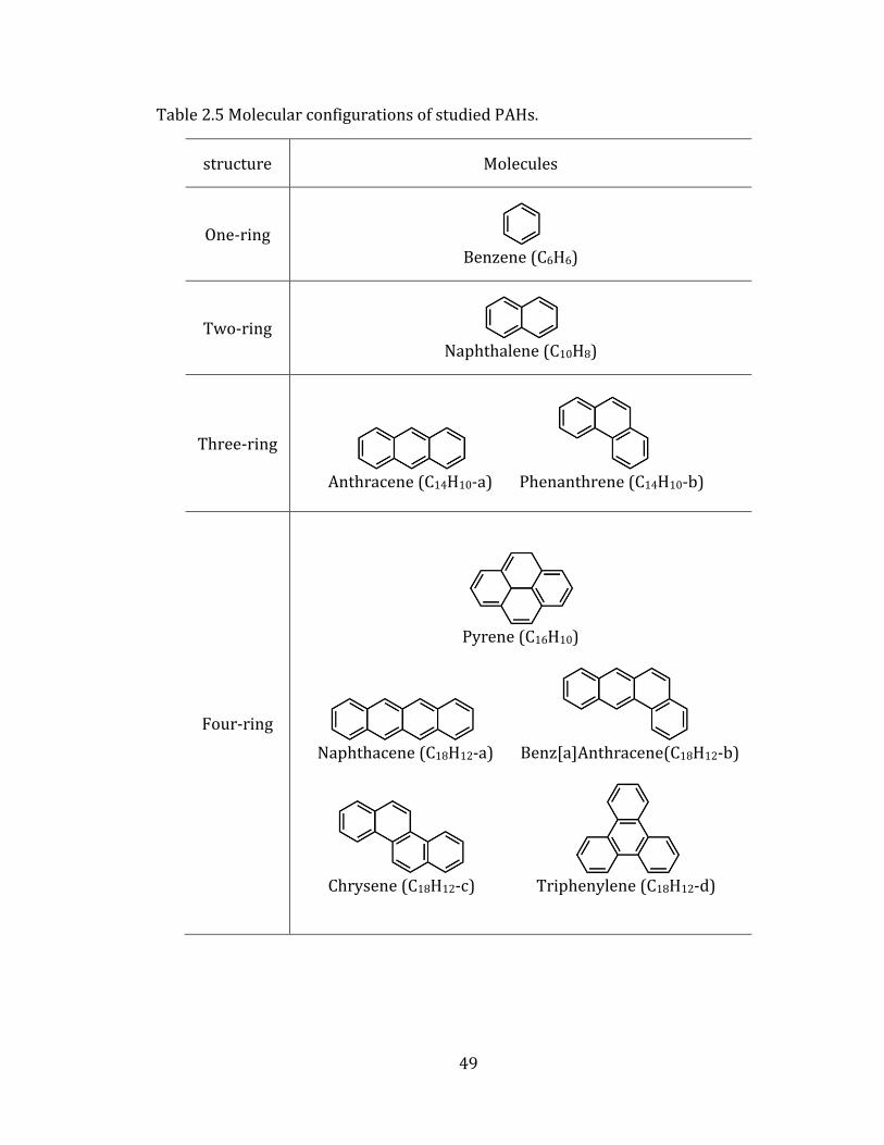
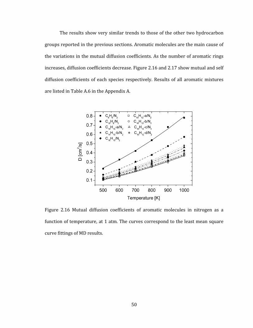
Figure 2.16 Mutual diffusion coefficients of aromatic molecules in nitrogen as a
function of temperature, at 1 atm. The curves correspond to the least mean square
curve fittings of MD results. ............................................................................................................. 50
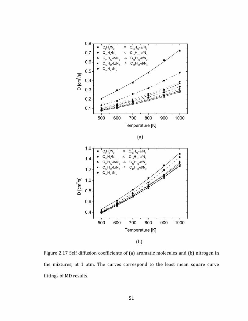
Figure 2.17 Self diffusion coefficients of (a) aromatic molecules and (b) nitrogen in
the mixtures, at 1 atm. The curves correspond to the least mean square curve
fittings of MD results. ......................................................................................................................... 51
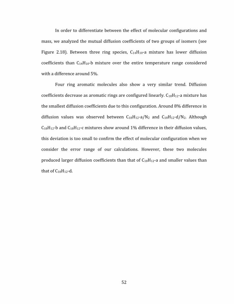
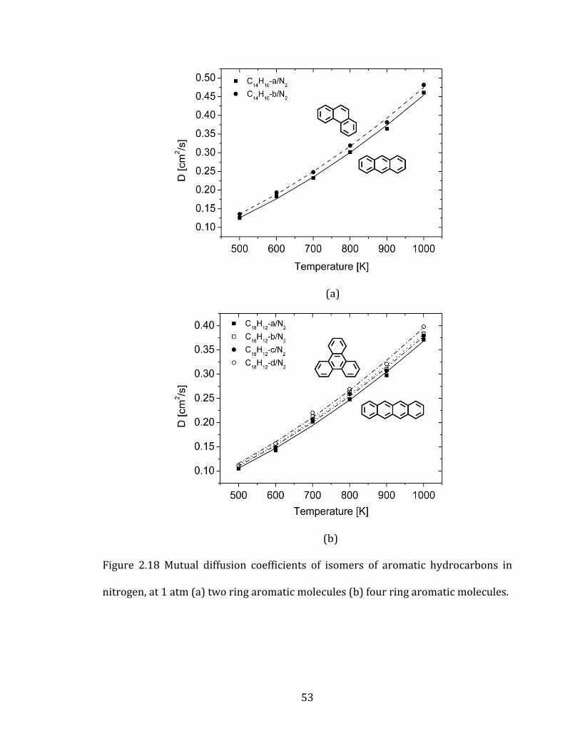
Figure 2.18 Mutual diffusion coefficients of isomers of aromatic hydrocarbons in
nitrogen, at 1 atm (a) two ring aromatic molecules (b) four ring aromatic molecules.
..................................................................................................................................................................... 53
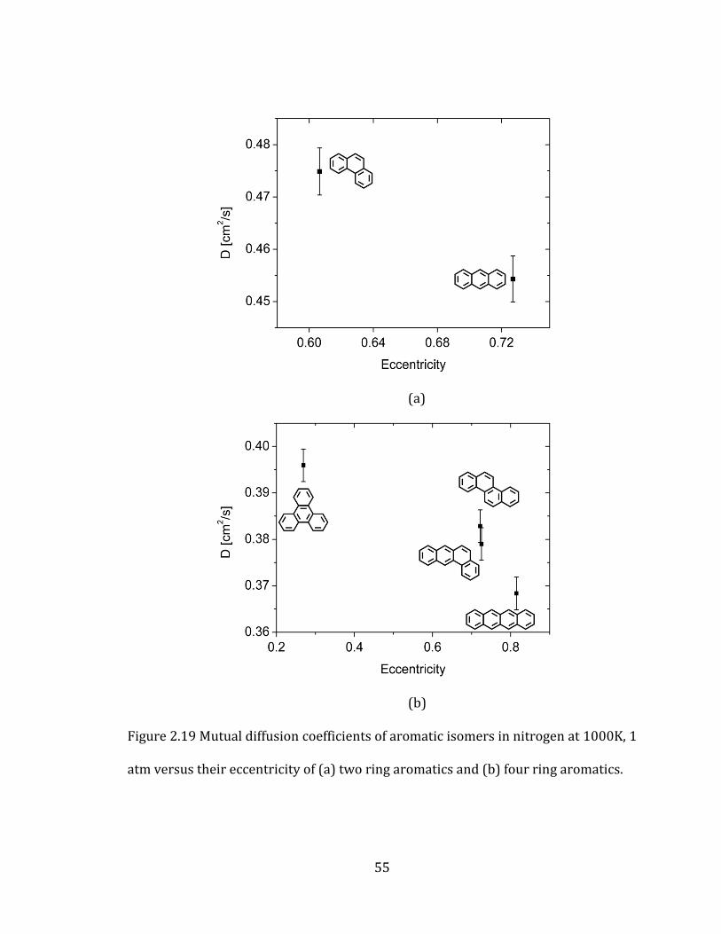
Figure 2.19 Mutual diffusion coefficients of aromatic isomers in nitrogen at 1000K,
1 atm versus their eccentricity of (a) two ring aromatics and (b) four ring aromatics.
..................................................................................................................................................................... 55
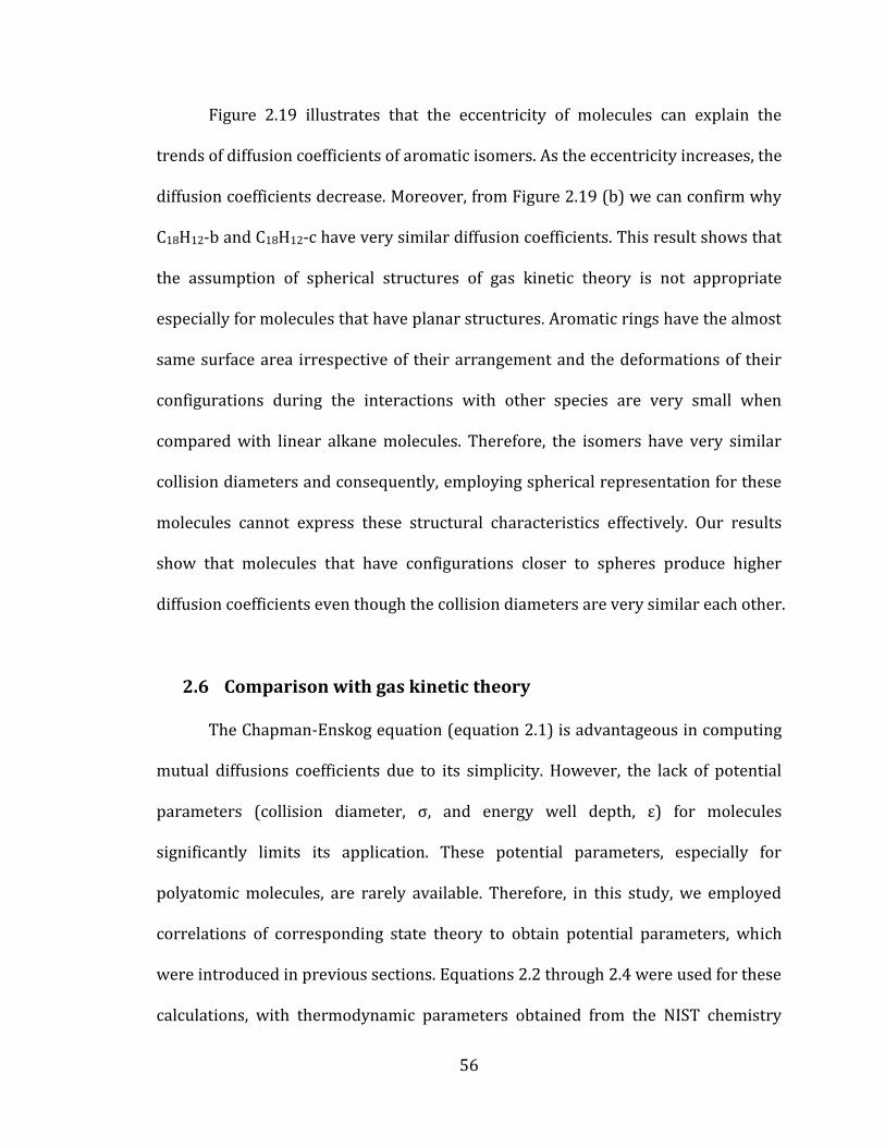
Figure 2.20 Mutual diffusion coefficients of linear alkanes in nitrogen as a function
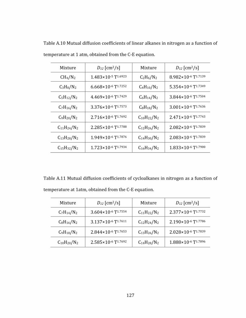
of temperature, at 1 atm obtained from the C-E equation. .................................................. 58
Figure 2.21 Comparison of mutual diffusion coefficients of (a) C2H6/N2, (b)
C6H14/N2, (c) C12H26/N2, and (d) C16H34/N2, at 1 atm (MD: Molecular dynamics
simulations, C-E: the Chapman-Enskog equation). ................................................................ 59
Page 12
x
Figure 2.22 Mutual diffusion coefficients of cycloalkanes in nitrogen as a function of
temperature, at 1 atm obtained from the C-E equation. ....................................................... 60
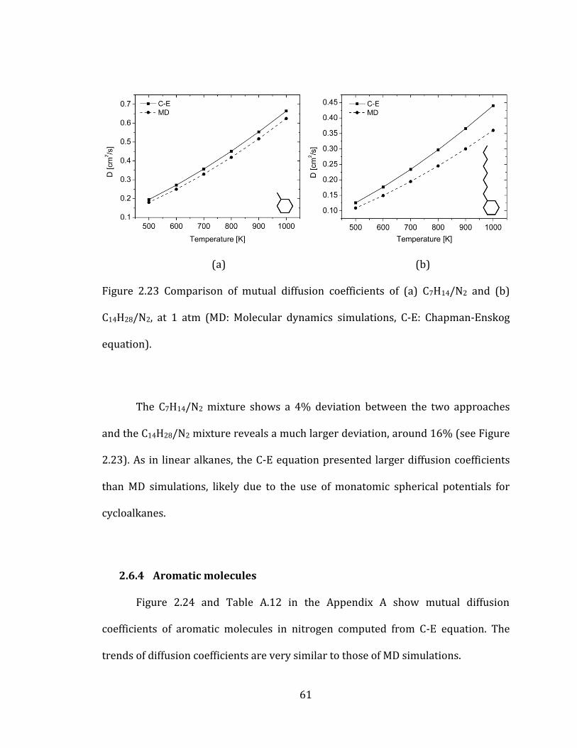
Figure 2.23 Comparison of mutual diffusion coefficients of (a) C7H14/N2 and (b)
C14H28/N2, at 1 atm (MD: Molecular dynamics simulations, C-E: Chapman-Enskog
equation). ................................................................................................................................................ 61
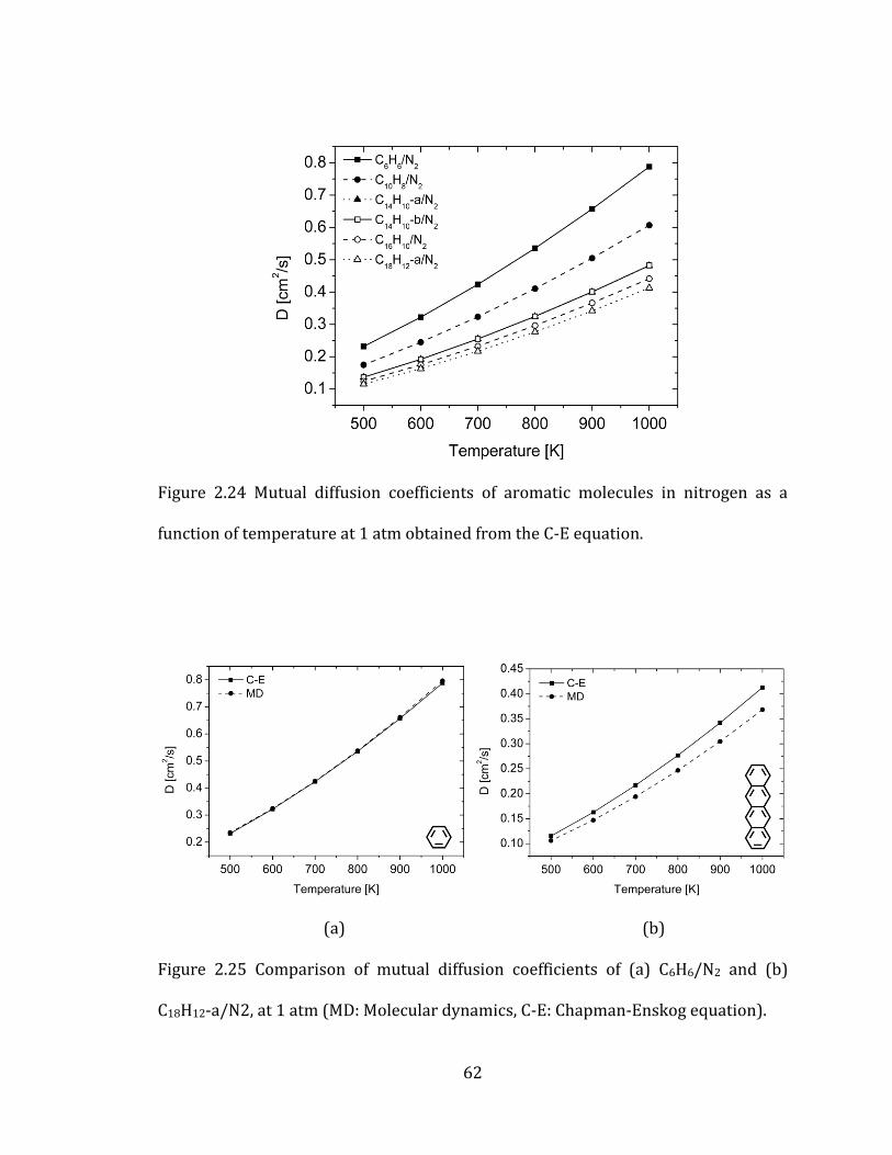
Figure 2.24 Mutual diffusion coefficients of aromatic molecules in nitrogen as a
function of temperature at 1 atm obtained from the C-E equation. ................................. 62
Figure 2.25 Comparison of mutual diffusion coefficients of (a) C6H6/N2 and (b)
C18H12-a/N2, at 1 atm (MD: Molecular dynamics, C-E: Chapman-Enskog equation).
.................................................................................................................................................................... .62
Figure 2.26 Collision diameters (σC-E) of linear alkanes obtained from the C-E
results and relations with average radius of gyrations (Rg). ............................................. 65
Figure 2.27 New collision diameters (σMD) of linear alkanes obtained from MD
results and relations with average radius of gyrations (Rg). ............................................. 67
Figure 2.28 Comparison of collision diameters of linear alkanes obtained from MD
and C-E results. Solid and dashed lines represent second-order fitting of σMD and σC-E
respectively. ........................................................................................................................................... 67
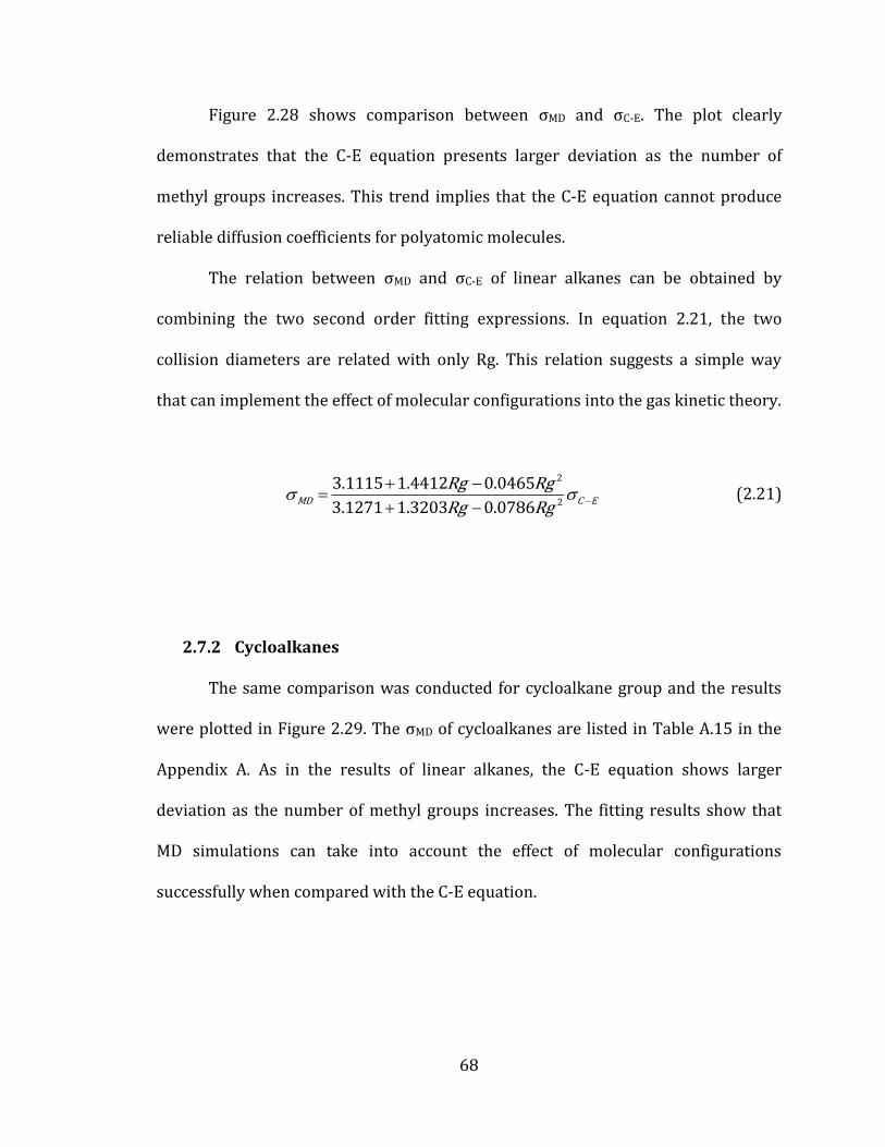
Figure 2.29 Comparison of collision diameters of cycloalkanes obtained from MD
and C-E results. Solid and dashed lines represent second-order fitting of σMD and σC-E
respectively. ........................................................................................................................................... 69
Page 13
xi
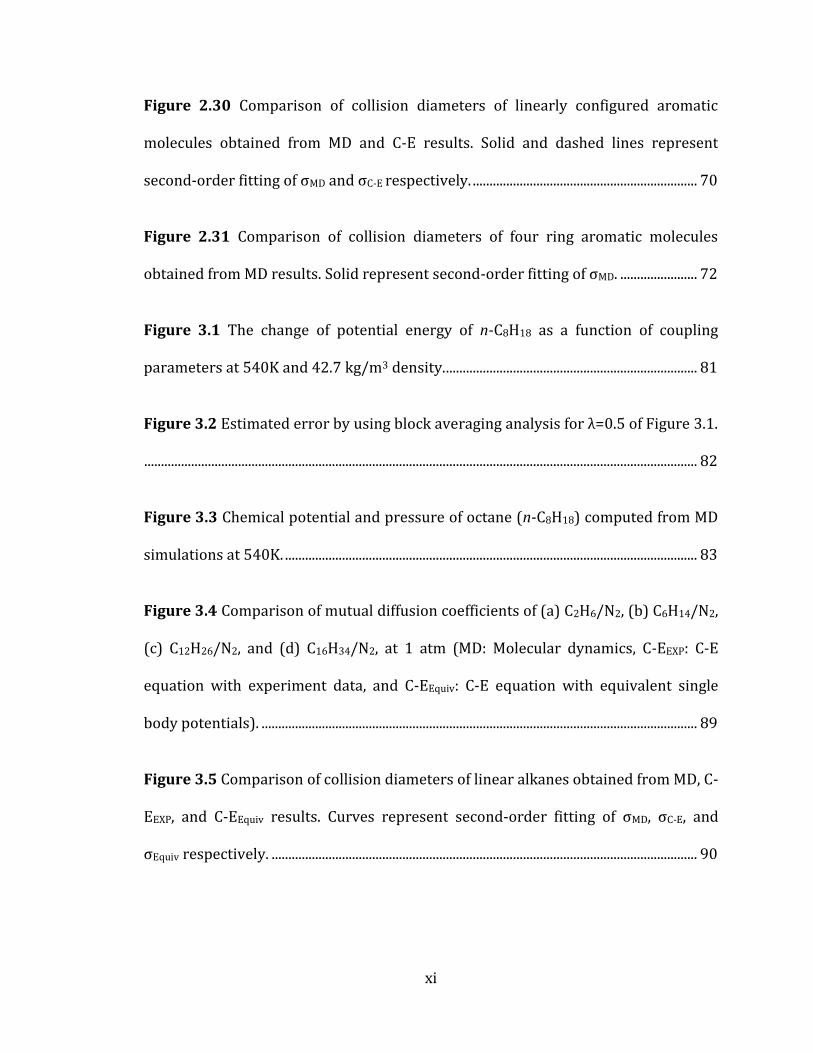
Figure 2.30 Comparison of collision diameters of linearly configured aromatic
molecules obtained from MD and C-E results. Solid and dashed lines represent
second-order fitting of σMD and σC-E respectively. ................................................................... 70
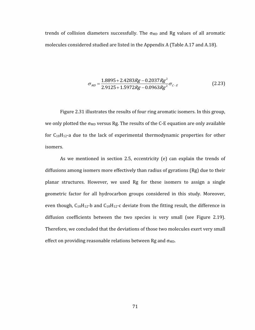
Figure 2.31 Comparison of collision diameters of four ring aromatic molecules
obtained from MD results. Solid represent second-order fitting of σMD. ....................... 72
Figure 3.1 The change of potential energy of n-C8H18 as a function of coupling
parameters at 540K and 42.7 kg/m3 density. ........................................................................... 81
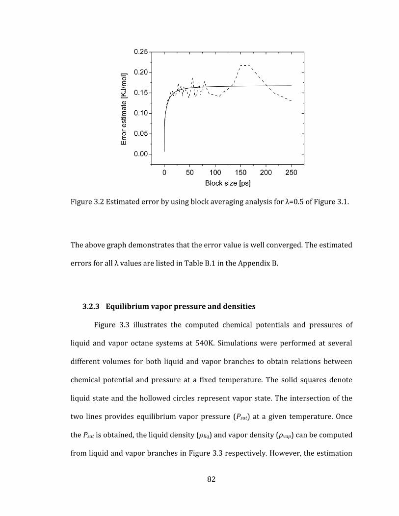
Figure 3.2 Estimated error by using block averaging analysis for λ=0.5 of Figure 3.1.
..................................................................................................................................................................... 82
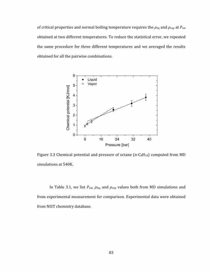
Figure 3.3 Chemical potential and pressure of octane (n-C8H18) computed from MD
simulations at 540K. ........................................................................................................................... 83
Figure 3.4 Comparison of mutual diffusion coefficients of (a) C2H6/N2, (b) C6H14/N2,
(c) C12H26/N2, and (d) C16H34/N2, at 1 atm (MD: Molecular dynamics, C-EEXP: C-E
equation with experiment data, and C-EEquiv: C-E equation with equivalent single
body potentials). .................................................................................................................................. 89
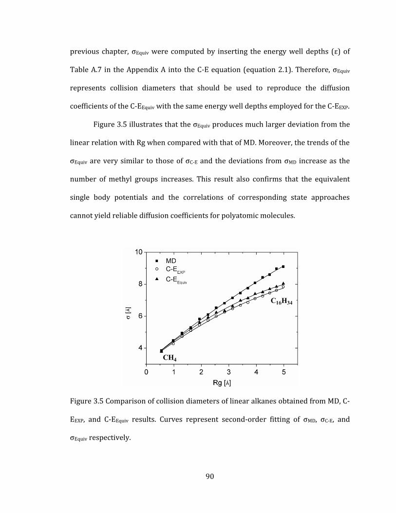
Figure 3.5 Comparison of collision diameters of linear alkanes obtained from MD, C-
EEXP, and C-EEquiv results. Curves represent second-order fitting of σMD, σC-E, and
σEquiv respectively. ............................................................................................................................... 90
Page 14
xii
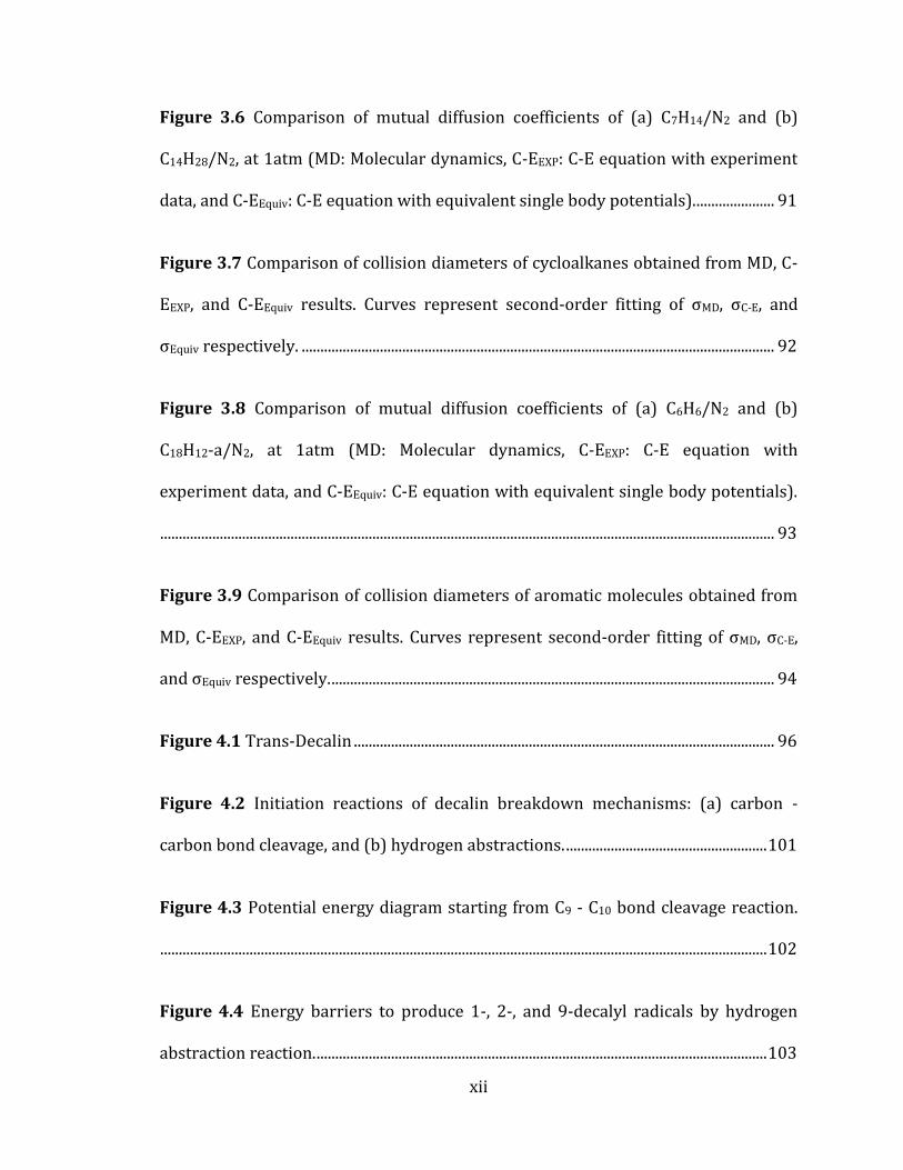
Figure 3.6 Comparison of mutual diffusion coefficients of (a) C7H14/N2 and (b)
C14H28/N2, at 1atm (MD: Molecular dynamics, C-EEXP: C-E equation with experiment
data, and C-EEquiv: C-E equation with equivalent single body potentials). ..................... 91
Figure 3.7 Comparison of collision diameters of cycloalkanes obtained from MD, C-
EEXP, and C-EEquiv results. Curves represent second-order fitting of σMD, σC-E, and
σEquiv respectively. ............................................................................................................................... 92
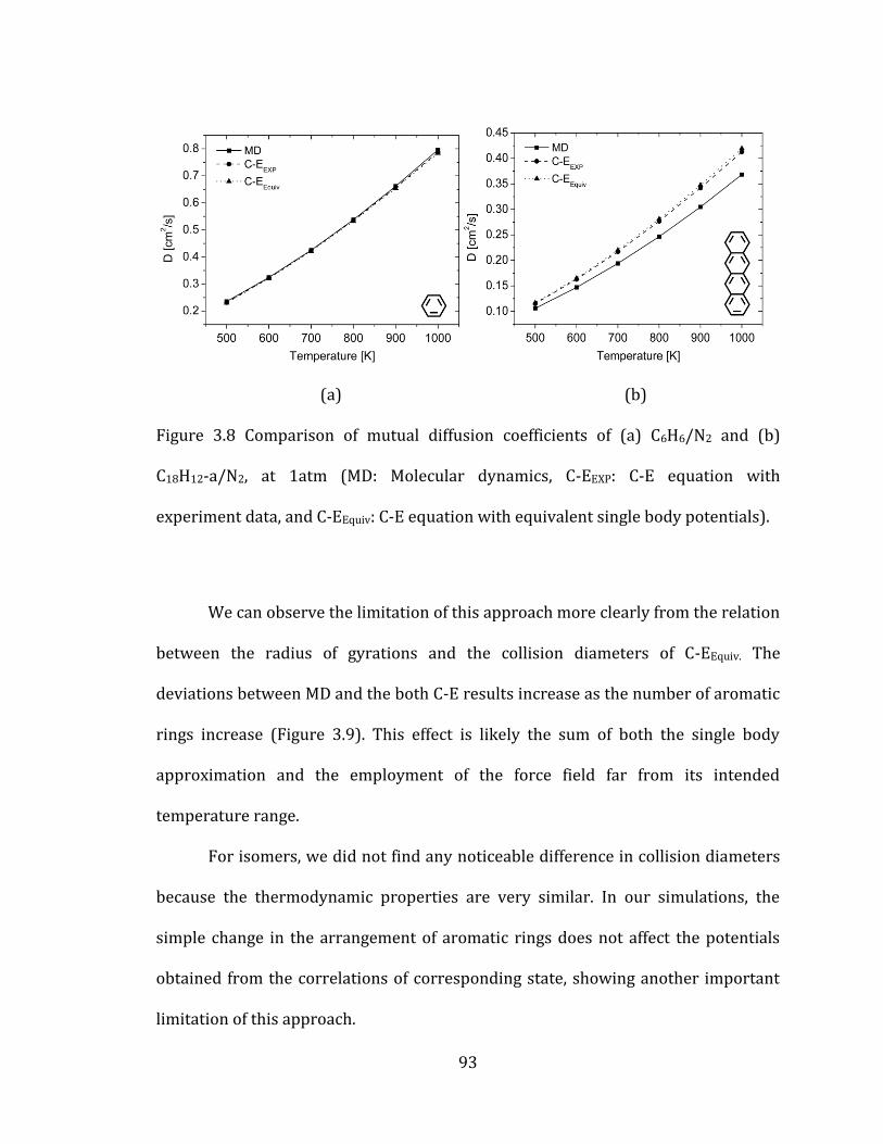
Figure 3.8 Comparison of mutual diffusion coefficients of (a) C6H6/N2 and (b)
C18H12-a/N2, at 1atm (MD: Molecular dynamics, C-EEXP: C-E equation with
experiment data, and C-EEquiv: C-E equation with equivalent single body potentials).
..................................................................................................................................................................... 93
Figure 3.9 Comparison of collision diameters of aromatic molecules obtained from
MD, C-EEXP, and C-EEquiv results. Curves represent second-order fitting of σMD, σC-E,
and σEquiv respectively. ....................................................................................................................... 94
Figure 4.1 Trans-Decalin ................................................................................................................. 96
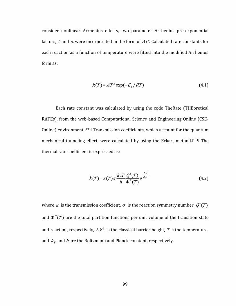
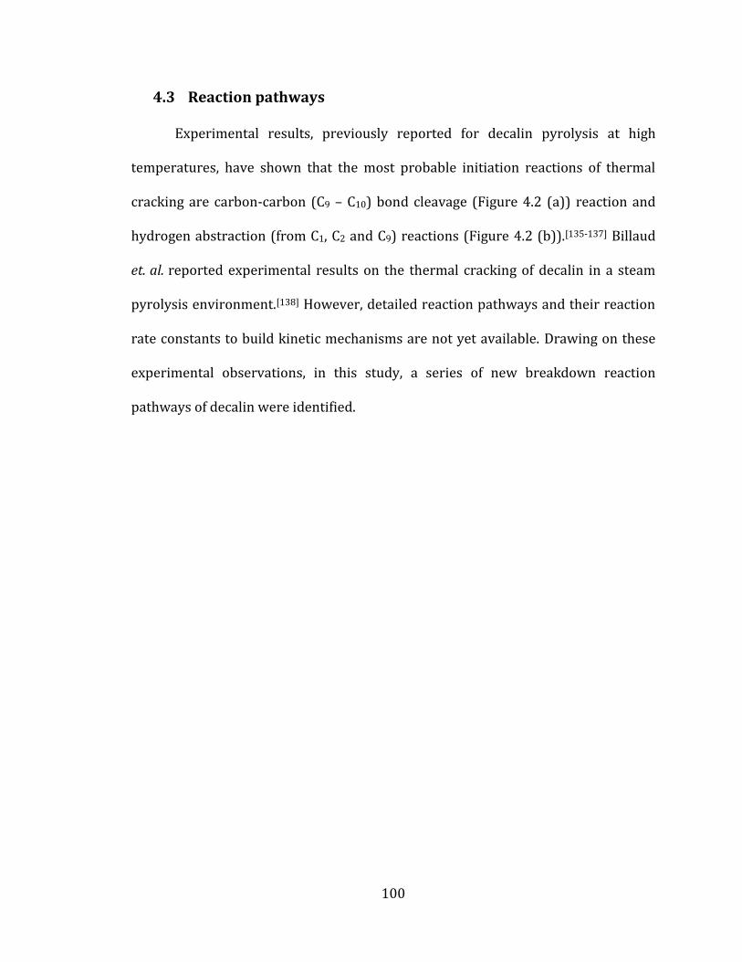
Figure 4.2 Initiation reactions of decalin breakdown mechanisms: (a) carbon -
carbon bond cleavage, and (b) hydrogen abstractions. ...................................................... 101
Figure 4.3 Potential energy diagram starting from C9 - C10 bond cleavage reaction.
................................................................................................................................................................... 102
Figure 4.4 Energy barriers to produce 1-, 2-, and 9-decalyl radicals by hydrogen
abstraction reaction. ......................................................................................................................... 103
Page 15
xiii
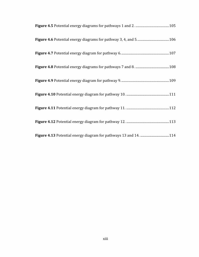
Figure 4.5 Potential energy diagrams for pathways 1 and 2. ......................................... 105
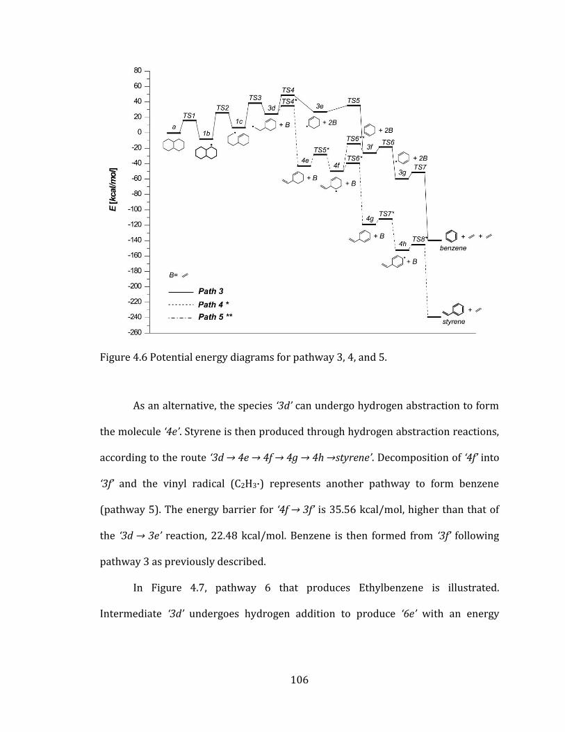
Figure 4.6 Potential energy diagrams for pathway 3, 4, and 5. ...................................... 106
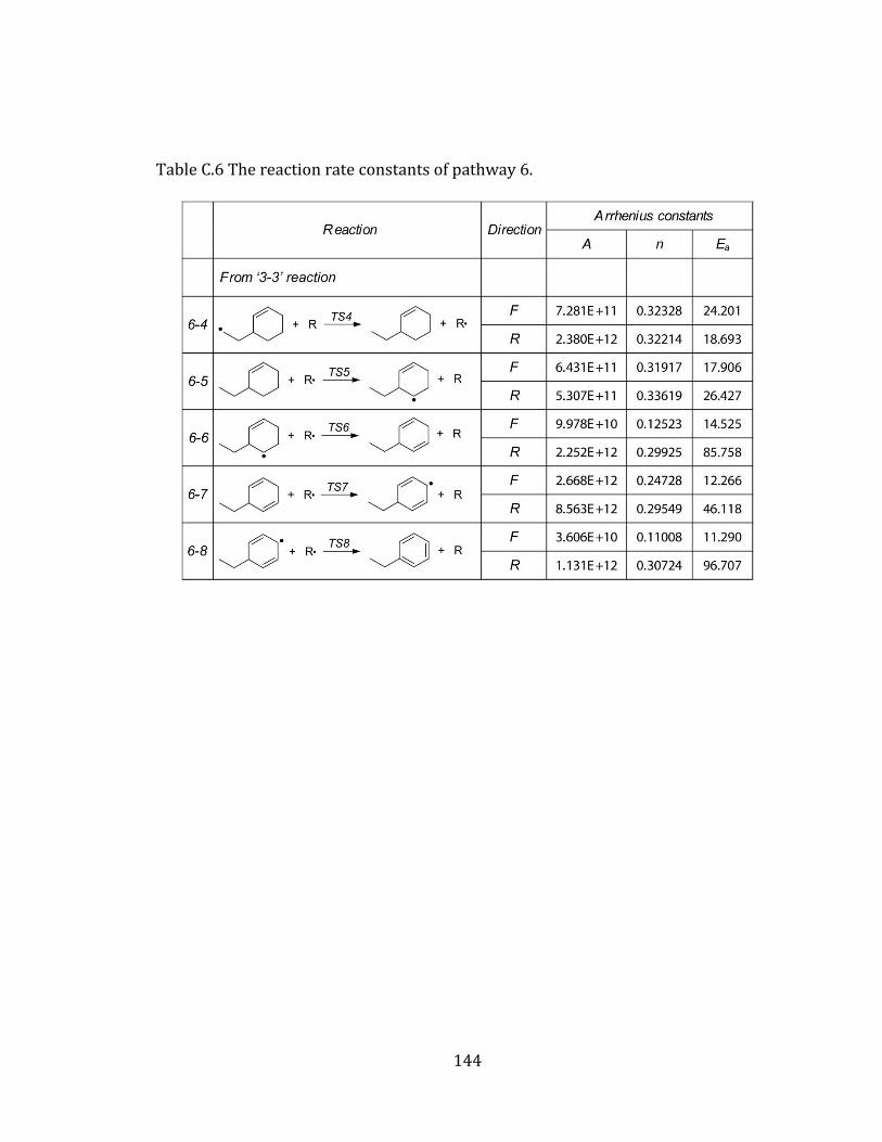
Figure 4.7 Potential energy diagram for pathway 6. .......................................................... 107
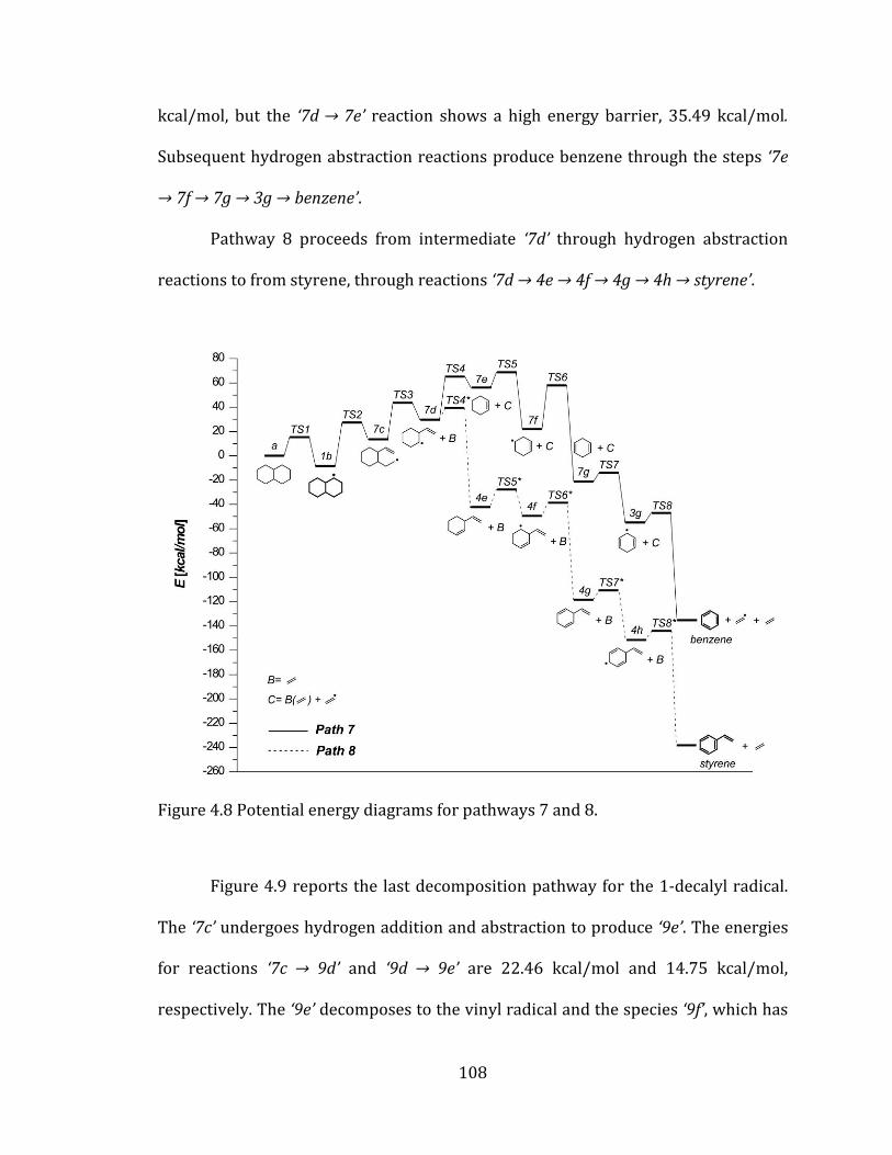
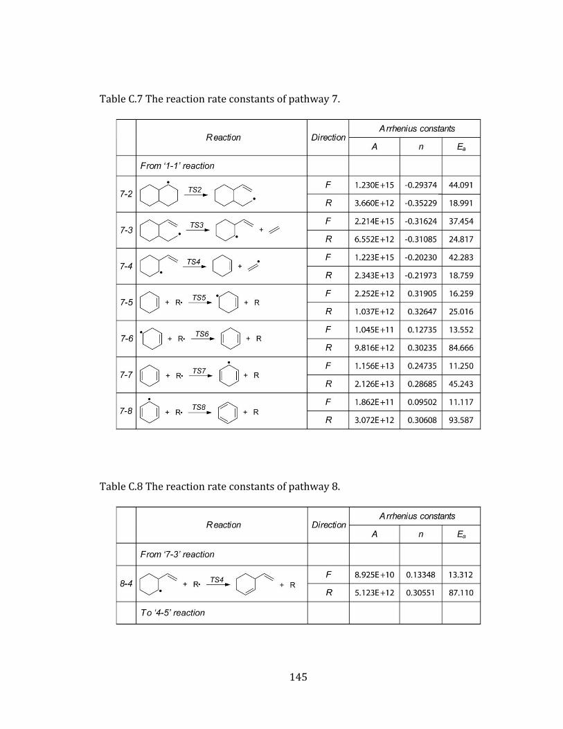
Figure 4.8 Potential energy diagrams for pathways 7 and 8. ......................................... 108
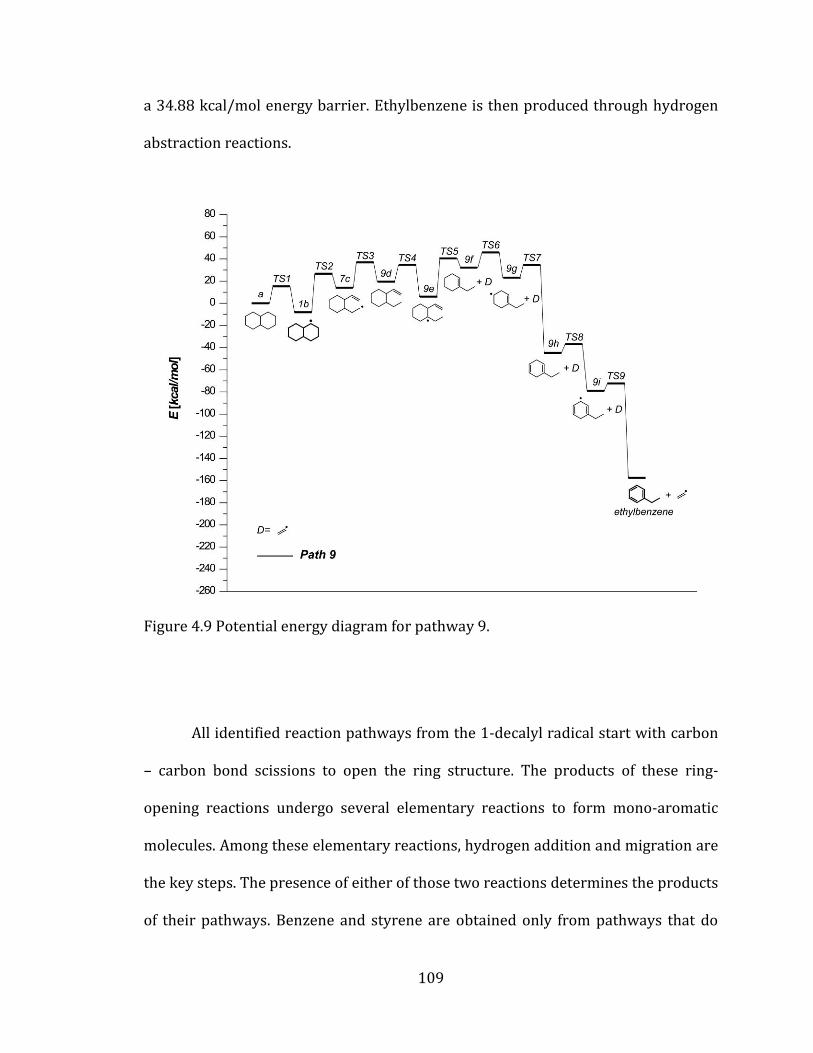
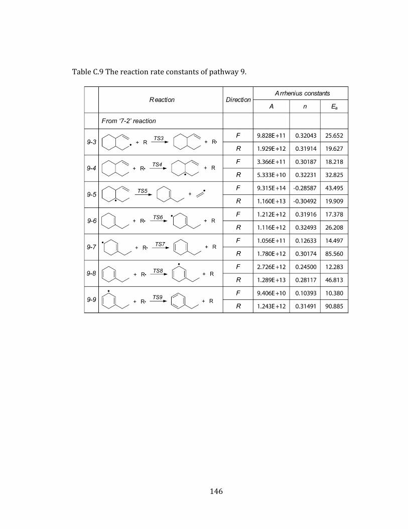
Figure 4.9 Potential energy diagram for pathway 9. .......................................................... 109
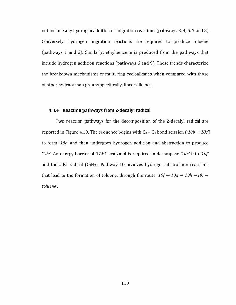
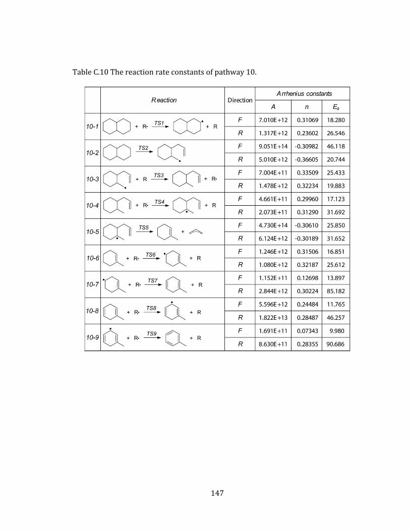
Figure 4.10 Potential energy diagram for pathway 10. .................................................... 111
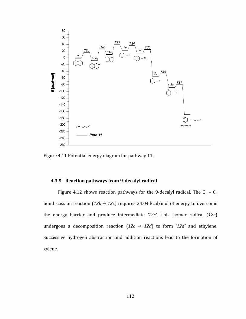
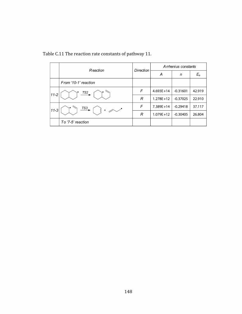
Figure 4.11 Potential energy diagram for pathway 11. .................................................... 112
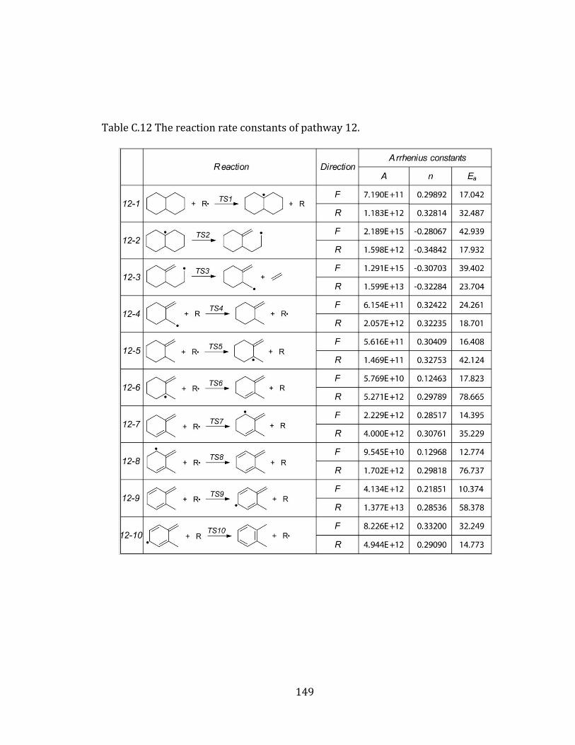
Figure 4.12 Potential energy diagram for pathway 12. .................................................... 113
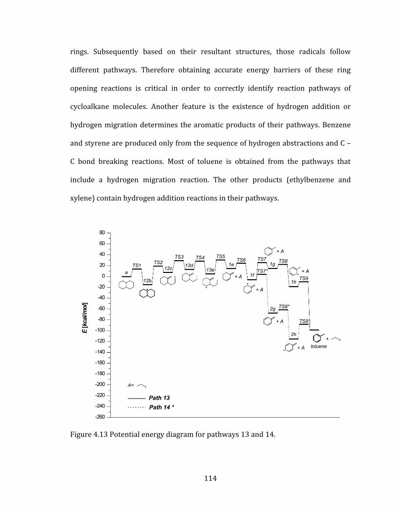
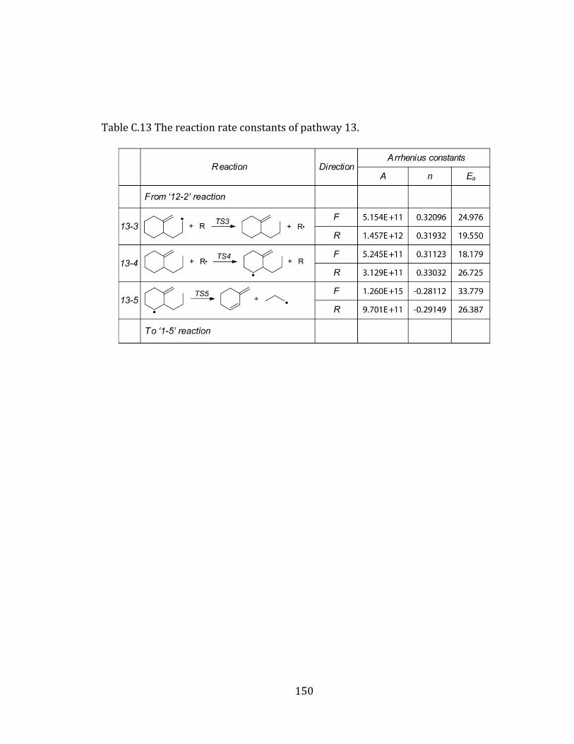
Figure 4.13 Potential energy diagram for pathways 13 and 14. ................................... 114
Page 16
xiv
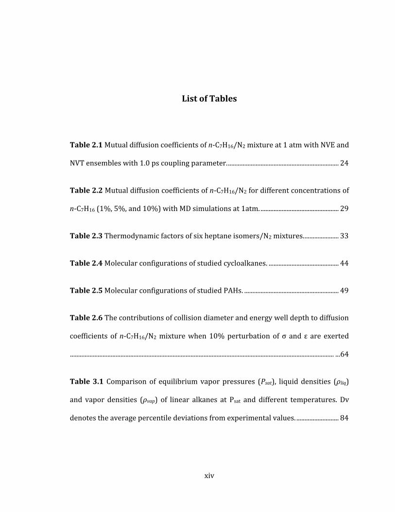
List of Tables
Table 2.1 Mutual diffusion coefficients of n-C7H16/N2 mixture at 1 atm with NVE and
NVT ensembles with 1.0 ps coupling parameter. .................................................................... 24
Table 2.2 Mutual diffusion coefficients of n-C7H16/N2 for different concentrations of
n-C7H16 (1%, 5%, and 10%) with MD simulations at 1atm. ................................................ 29
Table 2.3 Thermodynamic factors of six heptane isomers/N2 mixtures. ..................... 33
Table 2.4 Molecular configurations of studied cycloalkanes. ........................................... 44
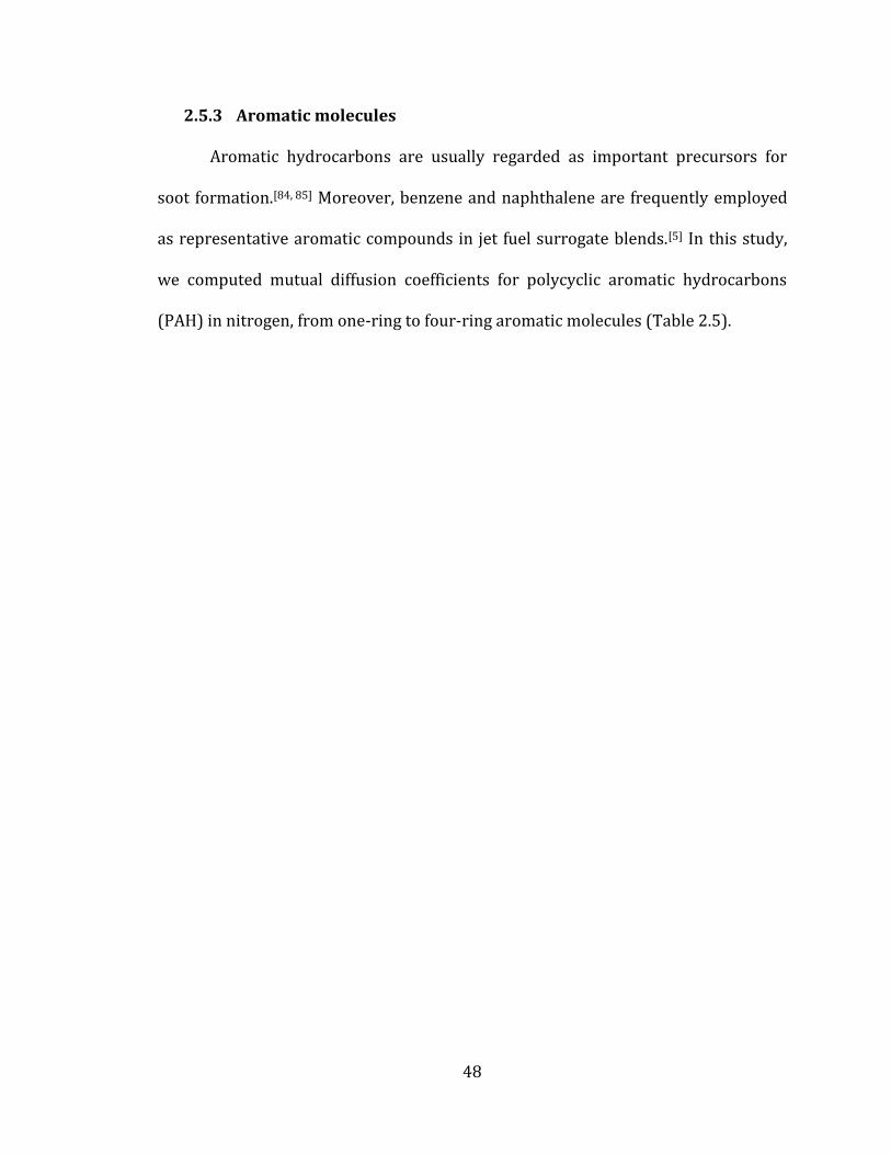
Table 2.5 Molecular configurations of studied PAHs. .......................................................... 49
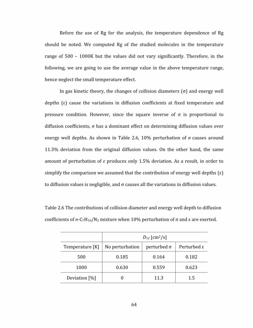
Table 2.6 The contributions of collision diameter and energy well depth to diffusion
coefficients of n-C7H16/N2 mixture when 10% perturbation of σ and ε are exerted
.................................................................................................................................................................. ...64
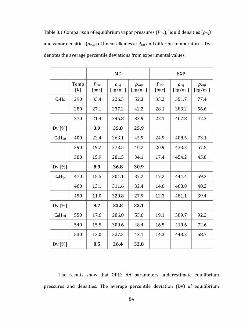
Table 3.1 Comparison of equilibrium vapor pressures (Psat), liquid densities (ρliq)
and vapor densities (ρvap) of linear alkanes at Psat and different temperatures. Dv
denotes the average percentile deviations from experimental values. .......................... 84
Page 17
xv
List of Appendices
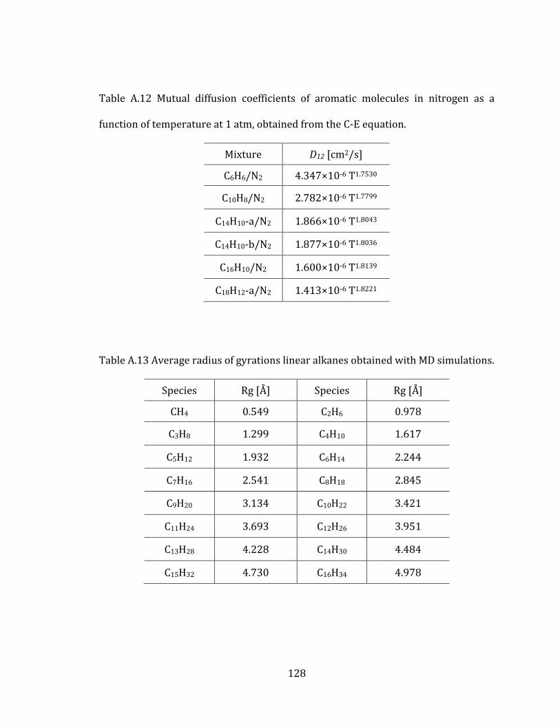
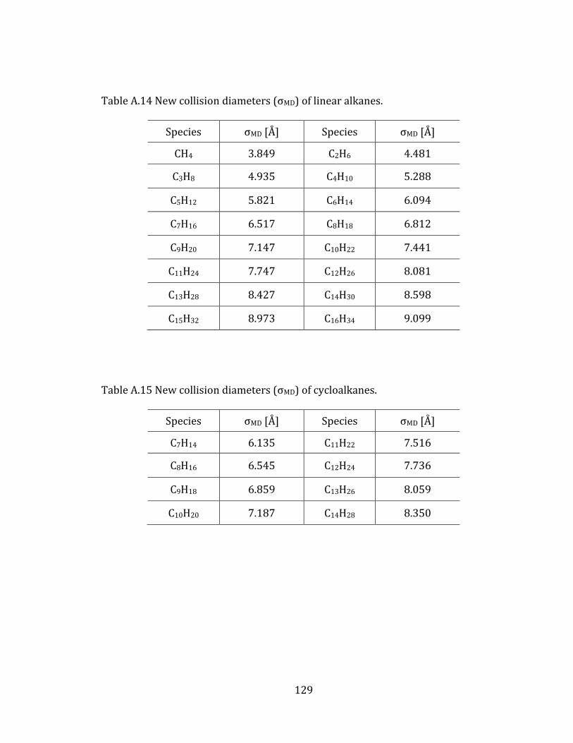
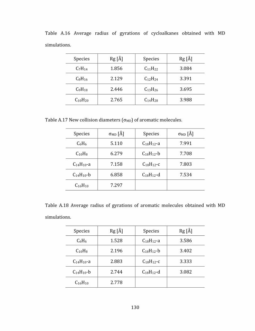
Appendix A. Supplementary tables of chapter 2………………………………………… 122
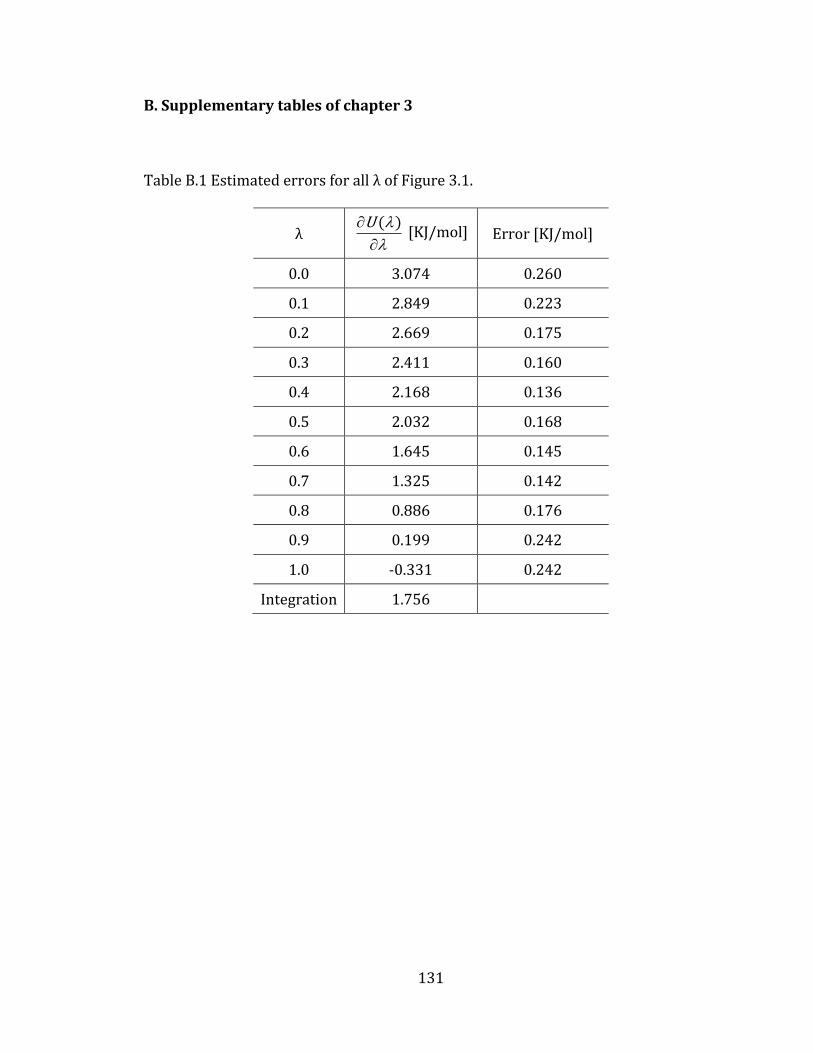
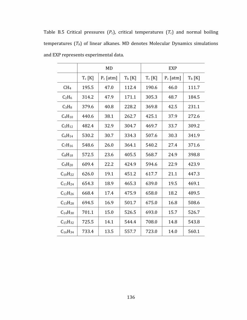
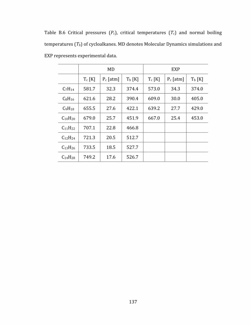
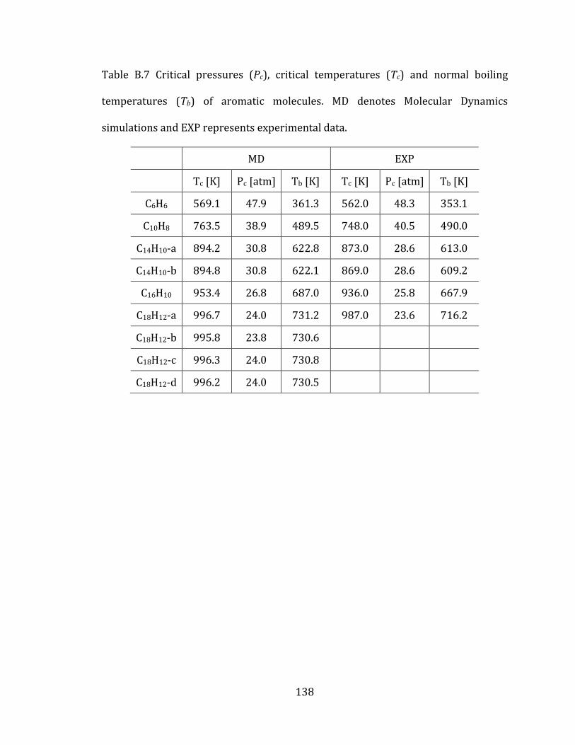
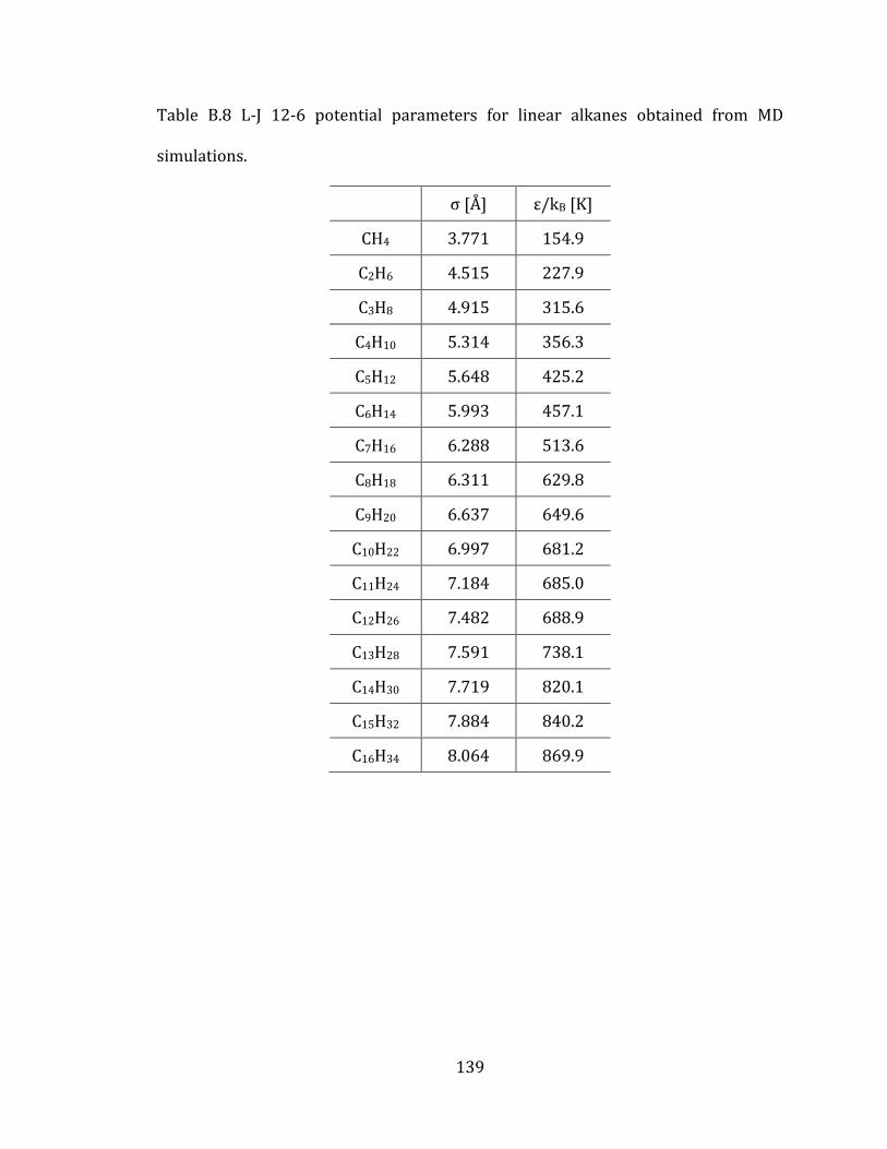
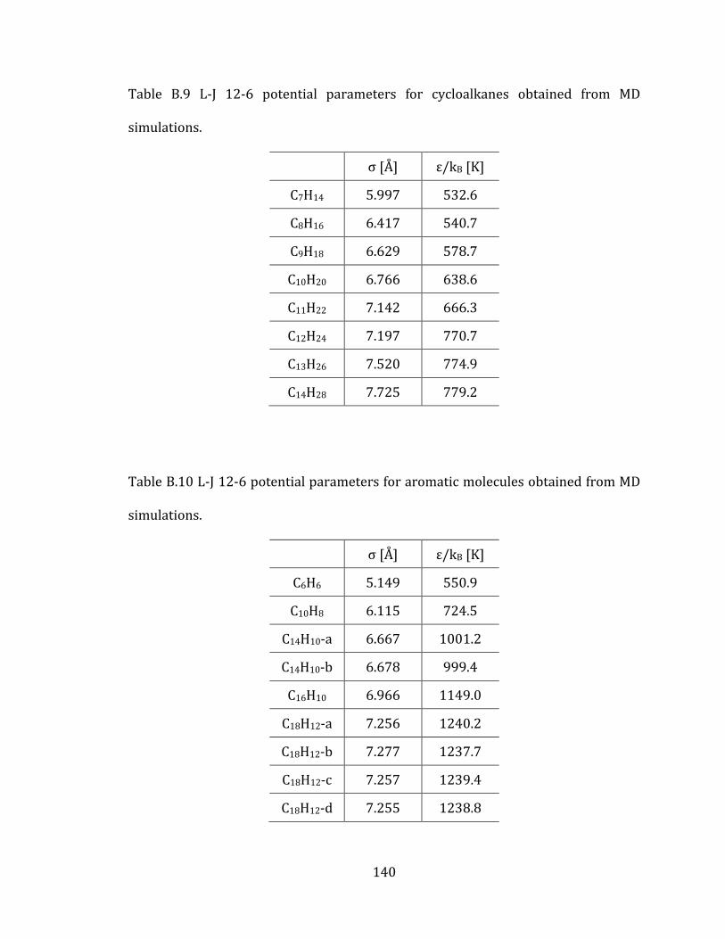
Appendix B. Supplementary tables of chapter 3……………………………………….… 131
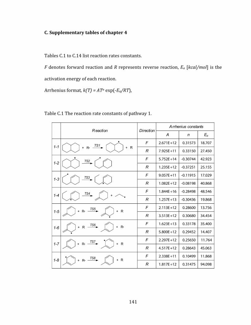
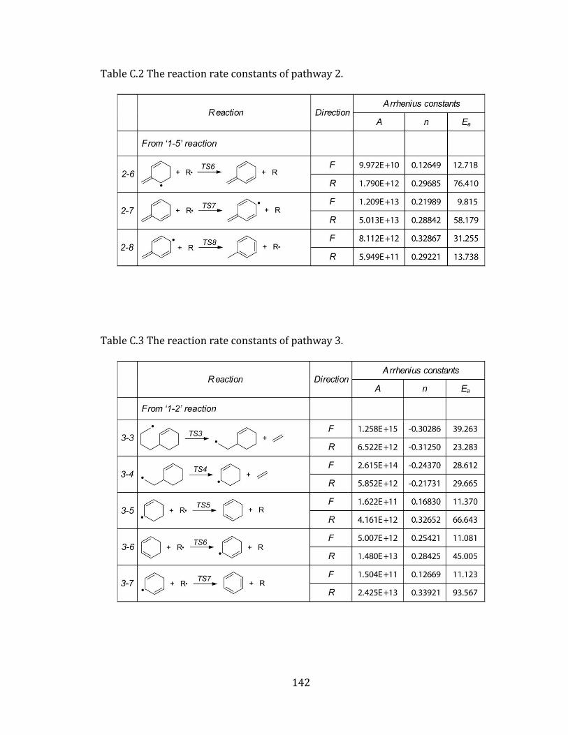
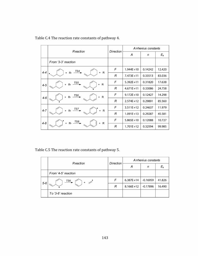
Appendix C. Supplementary tables of chapter 4….……………………………………… 141
Page 18
xvi
Abstract
The predictive capability of combustion modeling is directly related to the
accuracy of the models and data used for molecular transport and chemical kinetics.
In this work, we report on improvements in both categories.
The gas kinetic theory (GKT) has been widely used to determine the
transport properties of gas-phase molecules because of its simplicity and the lack of
experimental data, especially at high temperatures.
The major focus of this thesis is to determine the transport properties of
complex molecules and suggest an alternative way to overcome the limitations of
GKT, especially for large polyatomic molecules. We also recommend a correction
term to the expression of the diffusion coefficients that allows the expansion of the
validity of the GKT to include molecules with complex geometries and systems at
high temperatures. We compute the diffusion coefficients for three classes of
hydrocarbons (linear alkanes, cycloalkanes and aromatic molecules) using
Molecular Dynamics (MD) simulations with all-atom potentials to incorporate the
effects of molecular configurations. The results are compared with the values
obtained using GKT, showing that the latter theory overestimates the diffusion of
large polyatomic molecules and the error increases for molecules of significantly
non-spherical shape. A detailed analysis of the relative importance of the potentials
Page 19
xvii
used for MD simulations and the structures of the molecules highlights the
importance of the molecular shape in evaluating accurate diffusion coefficients. We
also proposed a correction term for the collision diameter used in GKT, based on the
radii of gyration of molecules.
In the field of chemical kinetics, we report on the reaction mechanisms for
the decomposition of decalin, one of the main components of jet fuel surrogates. We
identify fifteen reaction pathways and determine the reaction rates using ab-initio
techniques and transition state theory. The new kinetic mechanism of decalin is
used to study the combustion of decalin showing the importance of the new
reactions in predicting combustion products.
Page 20
1
Chapter 1
Introduction
1.1 Fuel surrogates
Computational combustion modeling is an essential tool not only for the
prediction of flame characteristics but also for the optimal design of combustors. In
the use of combustion modeling, conservation equations of fluid dynamics require
mass diffusion coefficients and chemical kinetic mechanisms as an essential input
data to investigate complex flame behaviors such as, flame speed, ignition
characteristics etc. Therefore, the predictive capability of computational modeling is
directly related to the accuracy of diffusion coefficients and kinetic mechanisms not
only of fuel components but also of other chemical species produced during
combustion.
Jet fuels are chemically complex mixtures that consist of a large variety of
molecules with different number of carbons and more than thousands of species.[1]
In recent years, reaction chemistry models have become more realistic and accurate
Page 21
2
to provide insight about complex interactions of reacting flow systems under
various temperature conditions. However, as the size of a molecule increases, the
number of chemical reactions and species grows rapidly. The size of detailed
reaction mechanisms for real fuel components is incredibly large and this
complexity requires huge computational resources to solve kinetic problems.
Therefore, it is not feasible to consider the reaction mechanisms of each single
component of complex fuels. Moreover, the kinetic mechanisms of all fuel
components are not well determined and the possible chemical kinetic interactions
among them are not clearly understood.
As a result, surrogate fuels composed of well known hydrocarbons, which
possess properties similar to those of target fuels, become attractive alternatives for
combustion applications.[2] Surrogate blends are comprised of a relatively small
number (less than ten species) of high purity hydrocarbons. Therefore, using
surrogate blends has the advantage of allowing fuel composition to be accurately
controlled.[3, 4]
The major categories of constituents of jet fuel are alkanes, cycloalkanes
(naphthenes), aromatics, and alkenes.[5] Alkanes (such as dodecane, tetradecane,
and isooctane) are the most abundant components and account for 50 – 60% by
volume. Cycloalkanes (such as methylcyclohexane, tetralin, and decalin) and
aromatics (such as toluene, xylene, and naphthalene) represent 20 – 30% by volume,
and alkenes account for less than 5%.
Simple fuel properties, such as hydrogen/carbon (H/C) ratio, can be readily
matched with a single-component surrogate.[6] However, other fuel properties, such
Page 22
3
as chemical composition, ignition delay, soot formation, and molecular transport
properties, usually require more components to be accurately reproduced.[6]
Although chemical kinetic mechanisms of hydrocarbons that comprise fuel
surrogates have been widely studied,[7-9] molecular transport data of those species,
especially for hydrocarbons that have large number of atoms, have not yet
experienced similar focus. Analytical equations derived from gas kinetic theory are
still widely used to compute mass diffusion coefficients for low density gas
combustion systems irrespective of the configurations of molecules. Consequently,
important questions about mass transport are being raised: How can diffusion
coefficients be determined, especially for polyatomic molecules with long chains
such as, dodecane (C12H26)? What is the effect of molecular shapes on diffusion
coefficients under high temperature reacting flow conditions? Can gas kinetic theory
be used for polyatomic molecules?
Recent advances in computational approaches, especially Molecular Dynamics
(MD) simulations, can overcome the problems of analytical approaches in
determining transport properties. In MD simulations, the configurations of
molecules can be considered by describing bonding and angle interactions of all
atoms that comprise polyatomic molecules. Molecular modeling techniques can
reveal discrepancy with the gas kinetic theory and provide an explicit way to
compute improved diffusion coefficients of polyatomic molecules.
The highlight of this study is twofold: first, we identified correlations
between molecular configurations and diffusion coefficients by using MD
simulations. Second, we suggested correction factors to gas kinetic theory for
Page 23
4
hydrocarbon classes. These corrections will provide a straightforward approach to
compute improved diffusion coefficients of large hydrocarbon molecules, as well as
new fuel components when both experimental measurement and theoretical
analysis are not feasible.
MD simulations will also provide new Lennard-Jones 12-6 potential
parameters, σ and ε, for each molecule, which can be directly applied to gas kinetic
theory for diffusion calculations. These parameters will be an improvement upon
existing data or will be completely novel for molecules in situations where this
information is unavailable.
1.2 Mass diffusion
Transport of macroscopic properties arises as a result of microscopic
molecular motions.[10] Transport processes occur when non-uniform spatial
distribution of macroscopic quantities such as, composition, temperature, and flow
velocity perturbs equilibrium states. The results of these molecular transport
processes appear as non equilibrium phenomena of mass diffusion, heat conduction,
and viscosity at macroscopic level.
For low density gas systems, free molecular motion, where the mean free path
of a molecule is much larger than the radius of the molecule, is dominant in flow
regions. As a result, molecules move freely and molecular collisions are described by
only binary interactions.[11] Gas kinetic theory is well established under this
condition, for molecules that have spherical structure such as, methane (CH4).
Page 24
5
Among transport properties, mass diffusion coefficients exert the biggest
influence on deciding the characteristics of low density gas combustion systems.
Mass diffusion results from the relaxation process of a state perturbed by a
concentration gradient, to an equilibrium state. It represents the mobility of each
species in fluid flow.[11] Diffusion coefficients are expressed by Fick’s law of diffusion
as:
J D C (1.1)
where D, the constant of proportionality, is the diffusion coefficient, J is the mass
flux, and C is the concentration gradient of a species in a fluid. The diffusion
coefficient is a property that related microscopic fluctuations to macroscopic flux
and it is generally a function of temperature and density of a fluid.
Diffusion coefficients are essential data to solve the species conservation
equation in flame modeling. In general, for a multicomponent combustion system,
we can assume that thermal or pressure induced diffusion are negligible.[12, 13]
Therefore, mass diffusion has a dominant effect on determining the balance among
the species in a reacting flow. Specifically, mutual mass diffusion coefficients
between nitrogen and fuel components critically influence flame characteristics.
1.2.1 The effect of mass diffusion on flame modeling
Flame modeling requires accurate mass diffusion coefficients over a wide
range of temperature and pressure conditions. Although several experiments and
Page 25
6
theoretical studies have been reported, most of the measurements were conducted
at relatively low temperatures (less than 500K).[14-20] Moreover, data on mass
diffusion still include considerable uncertainties. Therefore, the range of
applicability for combustion modeling is limited.[21]
In recent years, numerous theoretical and modeling studies have reported
the importance of mass diffusion coefficients in flame modeling.[22-26] H2/air flame
simulations, employing different transport formulations, produced between 15 – 30%
difference in predicted extinction strain rates.[25] Non-premixed flame modeling of
hydrocarbon surrogate fuels reported that the measured extinction strain rates are
related to the size and mobility of molecules. As the size of molecules decreases,
resistance to extinction strain rate increases.[1] Sensitivity analysis of ignition,
laminar flame speed and extinction strain rates to diffusion coefficients showed that
the sensitivity of diffusion is of the same order or larger than the ones of main
chemical reactions such as, H+O2 → O+OH.[25, 26]
Modeling of dodecane (n-C12H26) non-premixed flames showed that the
computed extinction strain rates were notably sensitive to the mutual diffusion
coefficients of normal dodecane and nitrogen in addition to those of oxygen and
nitrogen.[27] This result clearly implies that diffusion coefficients of fuel species are
critical in deciding extinction characteristics of non-premixed flames.
McEnally et al. studied co-flow laminar non-premixed flames and reported
the consumption rate of normal heptanes was slower than that of 2,2,3-
trimethylbutane in experiments.[28] This result is inconsistent with the main
consumption routes for heptanes. Hydrogen abstractions and carbon bond fission
Page 26
7
processes should consume 2,2,3-trimethylbutane less rapidly than normal
heptanes.[29] This inconsistency between the experimental evidence and kinetics
was caused by transport properties of the two isomers.
All the above studies show the importance of diffusion coefficients in
combustion modeling. However, the results only measured the effect of mass
diffusion in a qualitative manner. Those studies employed monatomic sphere model
to compute diffusion coefficients of polyatomic molecules in the frame of gas kinetic
theory. Moreover, none of these studies reported any method to improve the
accuracy of diffusion coefficient for combustion modeling. Therefore, alternative
approaches that can overcome the limitations in gas kinetic theory should be
proposed to improve predictive capability of combustion modeling and quantify the
effect on flame characteristics.
1.2.2 Approach for diffusion of polyatomic molecules
Gas kinetic theory utilizes a critical assumption that all molecules have
spherical structures to analyze the dynamics of molecular collisions. This approach
is reasonable and produces reliable diffusion coefficients for small molecules such
as, methane and nitrogen. However for large polyatomic molecules such as,
dodecane and hexadecane, the validity of the assumption is not obvious and needs
to be verified. Therefore, the first step to understand the limitations of gas kinetic
theory should be the incorporation of the effect of molecular configurations into
diffusion calculations by evaluating all interactions among atoms that comprise
molecules. Since constituents of hydrocarbon fuels typically have structures which
Page 27
8
deviate significantly from sphere, quantification of this effect on diffusion is needed
to improve the accuracy of diffusion coefficients.
For this purpose, we computed diffusion coefficients, taking into account
detailed molecular configurations, and proposed modifications to the gas kinetic
theory, which can be used for low density gas systems. To consider the detailed
morphology of molecules, we employed Molecular Dynamics (MD) simulations with
all-atom potentials. Atomistic level potentials can explicitly treat all bonding and
angle interactions within a molecule, as well as non-bonded interactions between
different molecules. As a result, our approaches can overcome the limitations of gas
kinetic theory and will provide an explicit way to compute diffusion coefficients of
polyatomic molecules.
MD simulations have been widely used to obtain diffusion coefficients of both
liquid and gas systems. However, results concerning the applications of MD to high
temperature systems have not yet been reported. Hence in this study we computed
diffusion coefficients of relatively high temperature gas systems by using MD
simulations. This work will produce molecular transport data applicable to
combustion modeling.
1.3 Kinetic mechanisms
Chemical kinetic mechanisms have been an essential part of combustion
modeling, ranging from simple flame burners to automotive engines and gas
turbines for aviation fuel combustion.[30-33] Typically, detailed kinetic mechanisms,
which consist of thousands of reactions, are too large to be solved in Computational
Page 28
9
Fluid Dynamics (CFD) models of real scale reacting flows. Therefore, reduced
chemical kinetic mechanisms, such as skeletal mechanisms[34, 35], are still commonly
used for all practical combustion modeling. Reduced kinetic models can be obtained
from validated detailed kinetic mechanisms to predict a range of experimental data.
In other words, reduced models should be optimized based on accurate chemical
reaction energies and reaction rates obtained from quantum chemistry technique or
experimental approaches. All possible reaction pathways of chemical species should
be identified before the reduced kinetic mechanisms are constructed. In recognition
of this need, detailed chemical kinetic mechanisms have been developed and
evaluated for various hydrocarbon fuel components by using ab-initio methods or
experimental measurements. Previous research has reported detailed reaction
mechanisms of normal alkane groups including n-heptane (n-C7H16) and its
isomers[36-38]; n-alkanes from n-octane (n-C8H18) to n-hexadecane (n-C16H34)[39];
aromatics including toluene (C7H8)[40]; and cycloalkanes including cyclohexane
(C6H12)[33] and methylcyclohexane (C7H14)[41]. These studies can provide extensive
information to build reduced kinetic mechanisms. However, detailed reaction
mechanisms of various aromatic molecules and especially cycloalkanes are still less
defined and are confined to small molecules because of their complex reaction
mechanisms and large number of possible reactions. Therefore, reaction pathways
of cycloalkanes should be constructed to improve the capability of predicting
combustion chemistry of fuel surrogates.
In recognition of this need, in this study, we will perform the analysis of
breakdown mechanisms of decalin (Decahydronaphthalene- C10H18), a reference
Page 29
10
component of multi-ring naphthene classes for jet fuel surrogate, by using Density
Functional Theory (DFT) method.
1.4 Outline
The objective of this thesis work is to develop a predictive model for the
combustion of jet fuels surrogate components. The major body of this study focuses
on determining the diffusion properties of complex hydrocarbons over a wide range
of temperatures using Molecular Dynamics simulations. Specifically, we will address
the effect of molecular structures on diffusion coefficients, and propose
implementations to the current models to take into account the geometry of
molecules.
In order to implement the kinetics of jet fuel surrogate, we use ab-initio
methods to determine reaction pathways of cycloalkanes, an important class of
compounds in jet fuel surrogates. The reaction model is then compared with
experimental data to assess the strength of the model in predicting important
combustion properties.
Brief descriptions of each chapter are presented below.
In chapter 2, basic theory of mass diffusion in low density gas conditions is
reviewed. A set of mathematical expressions are derived for mutual mass diffusion
coefficients in the frame of gas kinetic theory and statistical mechanics. After these
short review sections, mutual diffusion coefficients of hydrocarbon molecules in
Page 30
11
nitrogen are computed and the effect of molecular configurations is analyzed in the
following order.
First, comparison between MD simulations and available experimental data
is conducted to confirm the validity of MD simulations.
Second, heptane isomers are selected to test the capability of all-atom
potentials to capture the effect of molecular structures on diffusion
coefficients.
Third, mutual diffusion coefficients of normal alkanes, aromatic molecules,
and cycloalkanes in nitrogen carrier gas are computed with both MD
simulations and gas kinetic theory over the temperature range of 500 ~
1000K and at 1 atm pressure. The results are compared to show deviations
caused by using monatomic potentials or all-atom potentials for the same
molecules.
Finally, radius of gyration for target molecules is computed and compared to
collision diameters.
Chapter 3 reports on potential approaches that can eliminate the effect that
arises from using different potentials. Gas kinetic theory and MD simulations should
use potentials that have the same functional form to isolate the effect of molecular
configurations on mass diffusion coefficients. For this purpose, new molecular
potential parameters for gas kinetic theory were obtained by using atomistic MD
simulations.
Page 31
12
First, free energy calculations are conducted to compute chemical potential
of liquid and vapor states.
Second, based on chemical potential and pressure data, thermodynamic
properties, such as critical properties and boiling temperatures are
estimated.
Third, the correlation of corresponding state is applied to define new
molecular potential parameters from the thermodynamic properties. The
comparison is carried out between MD simulations and gas kinetic theory
with the molecular potential parameters.
Finally, we tested the relative contribution of molecular configurations and
force field to diffusion coefficients.
Chapter 4 describes the kinetic studies carried out for the cycloalkane class
of compounds in jet fuel surrogate. The potential energy surface is explored to
investigate the breakdown mechanism of Decalin (Decahydronaphthalene, C10H18), a
potential candidate of cycloalkane class for jet fuel surrogates. The Density
Functional Theory (DFT) method (B3LYP) is used to identify possible reaction
pathways. Rice-Ramsperger-Kassel-Marcus (RRKM) and Transition State Theory
(TST) are employed to compute high pressure limit reaction rate constants for the
identified reaction pathways. A kinetic analysis is also performed for pyrolysis
conditions to evaluate the importance of each reaction pathway.
In chapter 5, the highlights of the work are summarized.
Page 32
13
Chapter 2
Mutual diffusion coefficients of hydrocarbons in nitrogen
2.1 Investigation of mass diffusion
The most common approach to investigate the molecular transport of low
density gas systems is to use the Boltzmann transport equation of gas kinetic theory.
The solution of this transport equation, combined with Lennard-Jones potential
parameters, suggests a simple analytical expression for self and mutual diffusion
coefficients. This approach has been applied over wide range of flame modeling due
to the ease of use even though the theory was developed for only monatomic
molecules.[42]
2.1.1 Gas kinetic theory
Polyatomic molecules interact through the potentials between atomic
interacting sites located in each molecule. The major difficulties in the analysis of
binary collision between these molecules are the existence of inelastic collisions and
Page 33
14
the very complicated trajectories associated with angle dependent potentials.[11]
Kinetic theories for polyatomic gases were derived in three different ways. Taxman
suggested the classical kinetic theory.[42] Wang Chang and Uhlenbeck developed the
semi-classical theory which describes internal quantum states of a molecule as
separate chemical species so that the translational motion can be treated
classically.[43] Waldmann,[44] and Snider formulated fully quantum mechanical
kinetic theory.[45] However, direct application of these theories to compute diffusion
coefficients of polyatomic molecules is still too complex because of the difficulties in
assessing the dynamics of molecular collisions. Therefore, the analysis of collision
dynamics of polyatomic molecules should rely on the approximate method of
evaluating collision integrals that contain all of the information about interaction
energy related to intermolecular pair potentials and scattering mechanism of
molecular collisions.[11] The most widely used approximation scheme for evaluating
angular dependent interaction for transport properties has been proposed by
Mason and Monchick and Mason.[46] The authors computed collision integrals with
following assumptions:
1) Inelastic collisions have little effect on trajectories.
Most inelastic collisions involve the transfer of only one quantum
rotational energy and this amount of energy is much less than kBT.
However the translational kinetic energy is of the order of kBT.
2) In a given collision only one relative orientation is effective.
Although the potential acts along the whole trajectory, the deflection
angle is determined by the interaction in the closest distance of the
Page 34
15
colliding molecules. The relative orientation of two colliding molecules
does not change substantially.
3) Every possible orientation has equal weight
4) Quantum effects are neglected
These assumptions make the dynamics of a collision a mathematically manageable
problem. The collision integrals for a given pair of molecules are tabulated as a
function of the reduced temperature, *T . Based on these integrals, the Chapman-
Enskog solution to Boltzmann transport equation can give a simple mathematical
expression for mutual diffusion coefficients. Hirschfelder et. al. followed the
Chapman–Enskog approach, combined with the Lennard–Jones (L-J) 6 – 12
intermolecular potential function, and suggested the Hirschfelder–Bird–Spotz (HBS)
equation for mutual mass diffusion coefficients.[21]
312
12 2 (1,1)*12
( ) /(2 )3
8Bk T m
Dn
(2.1)
where kB is the Boltzmann constant; T is the temperature of a system; 12m is the
reduced mass of the pair components; n is the average number density; 12 is the
collision diameter of two species and (1,1)* is the collision integral. The collision
integral depends on the reduced temperature, *12/BT k T , where 12 is the
energy well depth of the intermolecular potentials. The main disadvantage of this
equation is the difficulty encountered in evaluating the collision diameter, 12 , and
Page 35
16
potential energy well depth, 12 . These two parameters are usually obtained from
viscosity measurements.[47] However, only limited amounts of measurement data
are available for polyatomic molecules. Therefore, the correlations of corresponding
states of Tee et al. are frequently employed to estimate the parameters for fluids.[48]
According to this theory, the volumetric behavior and the intermolecular
forces in a fluid can be characterized by critical pressure, Pc, critical temperature, Tc,
and acentric factor, ω, of the fluid. Therefore, the two potential parameters (σ and ε)
can be predicted from the three quantities.
1/3
1 1c
c
Pa b
T
(2.2)
2 2
B c
a bk T
(2.3)
where ‘a’ and ‘b’ are empirically derived coefficients and ω is an acentric factor that
measures non-sphericity of a molecule. The empirical coefficients are derived from
the viscosity and second virial coefficient data of 14 substances ranging from inert
gases to benzene and normal heptane.
1a = 2.3551, 1b = -0.3955, 2a = 0.8063, 2b = 0.6802
Lee and Kesler developed an analytical correlation, based on the 3-parameter
corresponding states principle for the acentric factor, ω.[49]
Page 36
17
6
6
ln( ) 5.927 6.096/ 1.288ln( ) 0.169
15.252 15.687/ 13.472ln( ) 0.436c br br br
br br br
P T T T
T T T
(2.4)
where /br b cT T T , Tb and Tc denote boiling and critical temperature respectively.
Typically, experimentally measured thermodynamic properties (Pc, Tc, and Tb) are
used for the above equations. However, the lack of these measurement data makes it
possible to apply the Chapman-Enskog (C-E) equation for only limited number of
molecules.
Another approach for molecular transport is to use atomistic modeling
techniques, such as Molecular Dynamics (MD) simulations. The main advantage of
this strategy over gas kinetic theory is that complete atomistic representation of a
molecule can be achieved by using molecular configuration data and all-atom
potentials. Therefore, MD simulations are especially useful for polyatomic molecules
that comprise fuel surrogate blends.
2.1.2 Green-Kubo formula and MD simulations
The fluctuation dissipation theorem, which is the basis of linear response
theory, suggests an advanced way to express the mass diffusion coefficient.[50-52] The
mathematical formulation of the theorem is expressed as the Green-Kubo (G-K)
relations.[50] This formula can determine diffusion coefficients from microscopic
fluctuations in systems at the equilibrium state instead of considering non-
Page 37
18
equilibrium systems.[53] As a result, this approach establishes a theoretical basis for
computing mass diffusion coefficients from equilibrium MD simulations.
The G-K formula expresses the self diffusion coefficient as the ensemble
average of the velocity auto correlation functions of time. The mutual mass diffusion
coefficient is defined as the combination of the ensemble average of velocity auto-
and cross-correlation functions of time. The cross correlation terms describe the
momentum transfer of a particle through its neighbors.[54] The mutual diffusion
coefficient is expressed as[55]
11 22 1212 2 1 1 2 1 2 2 2
1 2 1 2
2f f f
D Q x D x D x xx x x x
(2.5)
0
1( ) (0)
3i iD u t u dt
(2.6)
0
1( ) (0)
3i jf u t u dt
(2.7)
0
1( ) (0)
3f u t u dt
(2.8)
where D is the time integral of velocity auto-correlation functions of species α, u
and u are the velocity vectors of species α and β, f and f are the time integrals
of velocity cross-correlation function between the same species and between
species α and β respectively. x is the mole fraction of each species, while the
angular brackets denote the ensemble average. Q is a thermodynamic factor related
to the compositional derivative of chemical potential and corrects compositional
Page 38
19
dependence in diffusion flux.[56] The Q factor can be determined from the integral of
the radial distribution functions. For a binary mixture system, the parameter is
defined as[55]
1 2 11 22 12
1
1 2Q
x x
(2.9)
2
04 ( ) 1r g r dr
(2.10)
2
04 ( ) 1r g r dr
(2.11)
where ( )g r and ( )g r are the radial distribution functions between same
species and between species α and β respectively. and represent the spatial
integrals of the radial distribution functions. For a thermodynamically ideal mixture,
defined as the perfectly mixed state of a mixture, the integrals of the radial
distribution functions of each species are identical, and Q can be approximated as
unity.[57]
2.2 Computational method: Molecular Dynamics simulations
2.2.1 All-atom Force field
When using Molecular Dynamics (MD) simulations, potential parameters
used to describe intermolecular interactions between molecules are critical for
Page 39
20
predicting physical and chemical properties. Quantum mechanical approaches can
predict intermolecular potentials with accuracy but high computational cost limits
their applications to small systems. Therefore, molecular modeling approaches
typically employ empirical force fields.
The united atom (UA) model, in which a group of atoms are represented by a
single pseudo-atom, is computationally appealing and has been widely used in
predicting fluid properties.[58-60] However, reported results showed the inadequacy
of UA model.[61, 62] In those studies, self diffusion coefficients obtained by using the
UA model are too large due to the absence of hydrogen bonding and the smoother
potential energy surface that results from neglecting hydrogen atoms. The all-atom
model can resolve these issues by considering hydrogen atoms of hydrocarbons
explicitly and can provide an accurate description of the shape of molecules.
The OPLS AA force field, used in this study, is an empirical all atom force field
and can be applied for a wide range of hydrocarbon molecules.[63] This force field
has been widely used to obtain thermodynamic and transport properties of liquid
systems that consist of polyatomic molecules and the results of these studies
showed a good agreement with available experimental data.[64-68] However, the
validity of these potentials for low density gas systems should be addressed. The
parameters of OPLS AA potentials were optimized by matching liquid densities and
vaporization enthalpies of various hydrocarbon molecules near normal boiling
temperatures.[63] The accuracy of these parameters for high temperature low
density gas systems is still unknown. Therefore, we should test the capability of
Page 40
21
OPLS AA parameters, at least for high temperature gas diffusion calculations, by
comparison with available experimental data.
2.2.2 Potential model
The OPLS AA force field utilizes the Lennard-Jones (L-J) 12-6 potential model
for determining interatomic interactions between two atoms.
12 6
( ) 4 ij ijij iju r
r r
(2.11)
where r is the distance between two atoms; ij represents a separation distance at
which potential energy becomes zero; ij is the energy well depth of L-J potentials.
The interactions for unlike molecules are computed by using Lorentz-Berthelot
combining rules.[69, 70]
1( )
2ij i j ij i j (2.12)
All molecules were treated as fully flexible by allowing bond stretching and
angle vibration, as well as the change of torsion angle. Bond stretching and angle
vibration were represented by harmonic potentials
Page 41
22
2
0
1
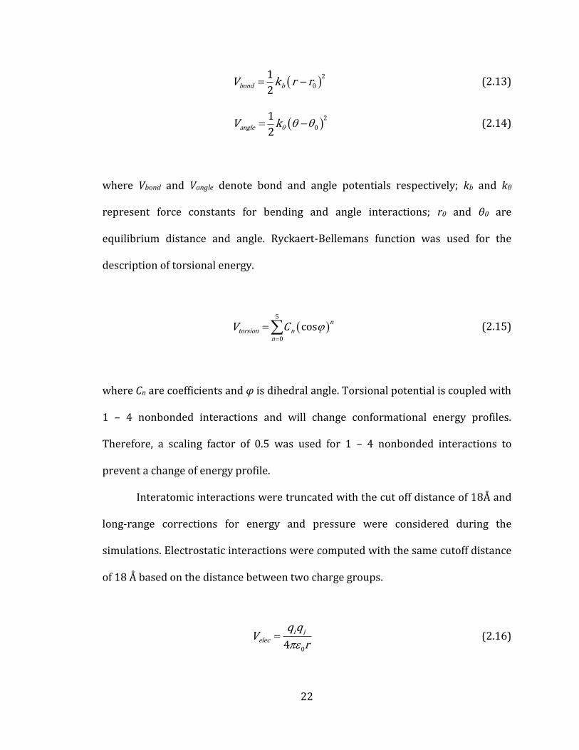
2bond bV k r r (2.13)
2
0
1
2angleV k (2.14)
where Vbond and Vangle denote bond and angle potentials respectively; kb and kθ
represent force constants for bending and angle interactions; r0 and θ0 are
equilibrium distance and angle. Ryckaert-Bellemans function was used for the
description of torsional energy.
5
0
cosn
torsion nn
V C
(2.15)
where Cn are coefficients and φ is dihedral angle. Torsional potential is coupled with
1 – 4 nonbonded interactions and will change conformational energy profiles.
Therefore, a scaling factor of 0.5 was used for 1 – 4 nonbonded interactions to
prevent a change of energy profile.
Interatomic interactions were truncated with the cut off distance of 18Å and
long-range corrections for energy and pressure were considered during the
simulations. Electrostatic interactions were computed with the same cutoff distance
of 18 Å based on the distance between two charge groups.
04
i jelec
q qV
r (2.16)
Page 42
23
where q is partial charge of an atom and ε0 is the permittivity of vacuum.
2.2.3 Simulation method
Simulations were conducted in the temperature range of 500 ~ 1000K and 1
atm pressure. The initial position of each atom is achieved by placing them arbitrary
position in a simulation box and the initial velocity of each atom was generated with
a Maxwellian distribution at a give temperature. Total simulation time was 14ns and
velocity components of each atom were recorded every 50 time steps. The force
acting on each atom was calculated with Newton’s equation of motion and given
force field. To integrate the equation of motion, the verlet leapfrog numerical
algorithm was used with a time step of 1.0 fs. All MD simulations were carried out
with the GROMACS software packages.[71]
In defining system sizes, we used experimentally measured densities at each
temperature and utilized periodic boundary conditions of cubic box. The canonical
ensemble (NVT) was obtained by employing a global Nose-Hoover global
thermostat.[72, 73]
2.2.4 The effect of the thermostat
Nose-Hoover thermostat controls temperature by expanding phase space
with scaled momentum.[74] The velocity components of particles can be perturbed
by this scaling method. Therefore, computing transport properties requires a very
weak perturbation so that the thermostat exerts negligible influence on the final
Page 43
24
results. Studies of self and binary diffusion coefficients of pure liquids such as N2,
CO2, C2H6, and C2H4 showed that the Nose-Hoover global thermostat did not
influence significantly the values of diffusion coefficients.[75] However, the effect of
thermostat on transport properties in high temperature gas systems has not been
addressed. Therefore, we compared the results of NVE ensemble with those of NVT
ensemble to identify the effect of the thermostat on diffusion coefficients. Normal
heptane and nitrogen (n-C7H16/N2) mixtures were used and simulations were
performed at two different temperature conditions (500K and 1000K) as the
strength of the temperature coupling varies. The coupling strength of the Nose-
Hoover global thermostat is expressed with the period of the oscillations of kinetic
energy between the systems and the reservoir. Short oscillation times produce
strong coupling and vice versa.
Table 2.1 Mutual diffusion coefficients of n-C7H16/N2 mixture at 1 atm with NVE and
NVT ensembles with 1.0 ps coupling parameter.
D12 [cm2/s]
Temp. NVT NVE
500K 0.172 ± 0.005 0.173 ± 0.007
1000K 0.557 ± 0.013 0.558 ± 0.016
Page 44
25
(a) (b)
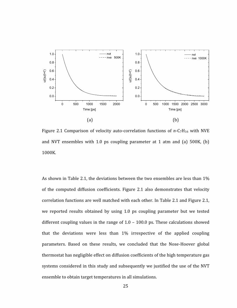
Figure 2.1 Comparison of velocity auto-correlation functions of n-C7H16 with NVE
and NVT ensembles with 1.0 ps coupling parameter at 1 atm and (a) 500K, (b)
1000K.
As shown in Table 2.1, the deviations between the two ensembles are less than 1%
of the computed diffusion coefficients. Figure 2.1 also demonstrates that velocity
correlation functions are well matched with each other. In Table 2.1 and Figure 2.1,
we reported results obtained by using 1.0 ps coupling parameter but we tested
different coupling values in the range of 1.0 – 100.0 ps. These calculations showed
that the deviations were less than 1% irrespective of the applied coupling
parameters. Based on these results, we concluded that the Nose-Hoover global
thermostat has negligible effect on diffusion coefficients of the high temperature gas
systems considered in this study and subsequently we justified the use of the NVT
ensemble to obtain target temperatures in all simulations.
Page 45
26
2.2.5 Velocity correlation
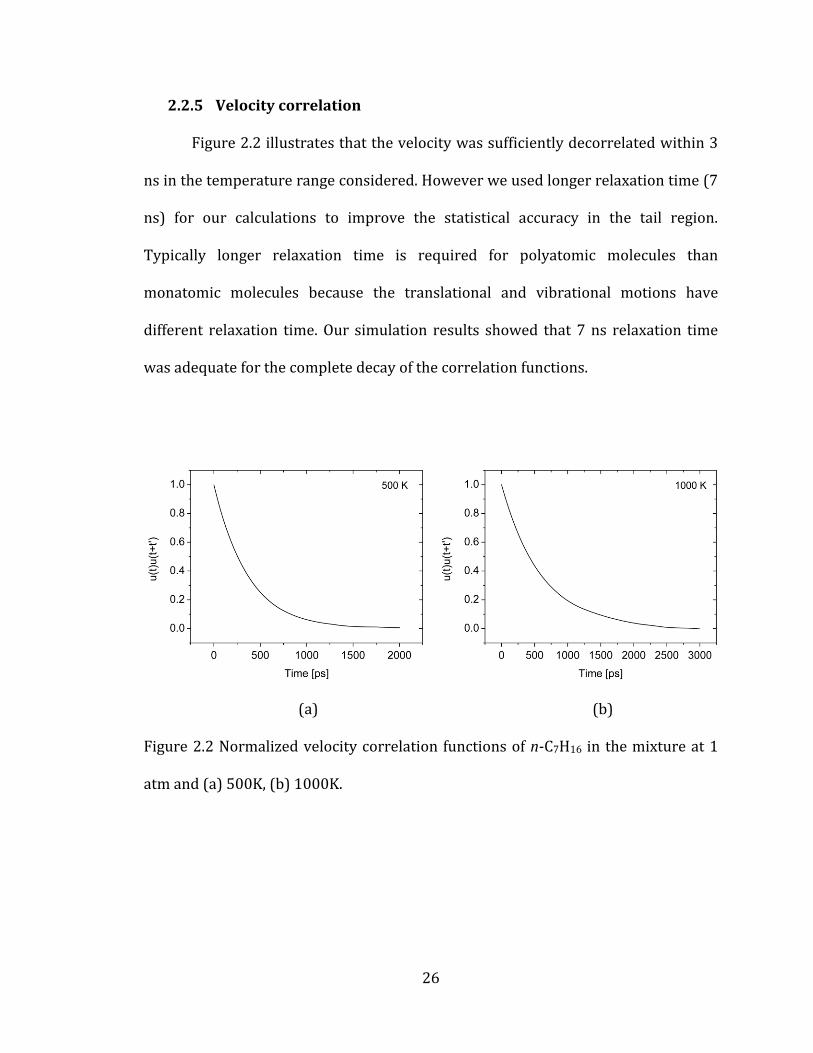
Figure 2.2 illustrates that the velocity was sufficiently decorrelated within 3
ns in the temperature range considered. However we used longer relaxation time (7
ns) for our calculations to improve the statistical accuracy in the tail region.
Typically longer relaxation time is required for polyatomic molecules than
monatomic molecules because the translational and vibrational motions have
different relaxation time. Our simulation results showed that 7 ns relaxation time
was adequate for the complete decay of the correlation functions.
(a) (b)
Figure 2.2 Normalized velocity correlation functions of n-C7H16 in the mixture at 1
atm and (a) 500K, (b) 1000K.
Page 46
27
2.3 Benchmark of computational approaches
2.3.1 The effect of system size
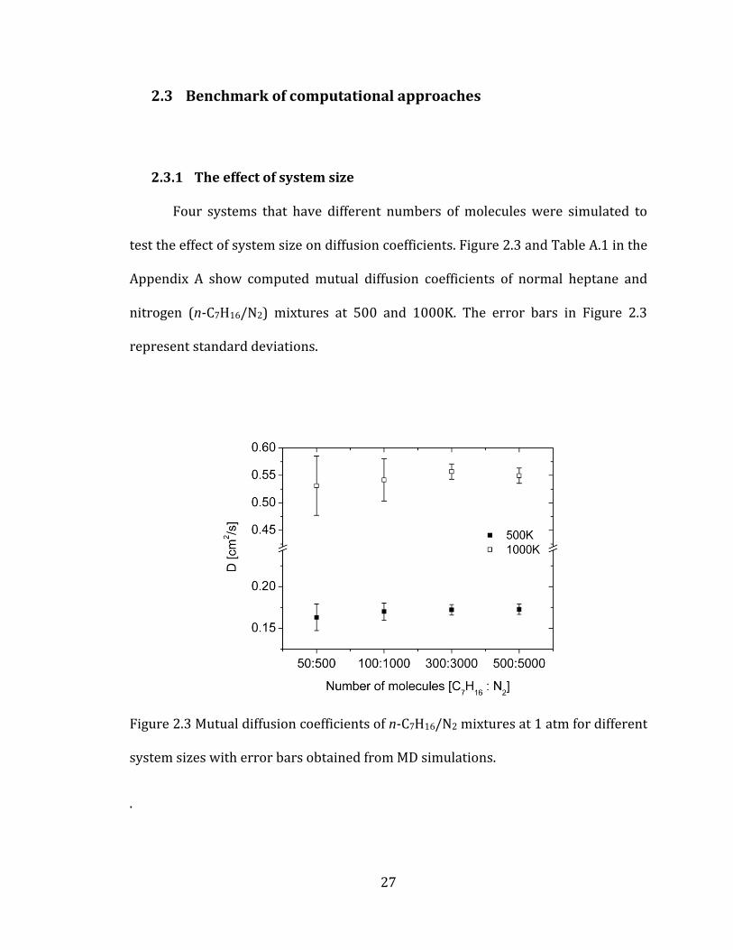
Four systems that have different numbers of molecules were simulated to
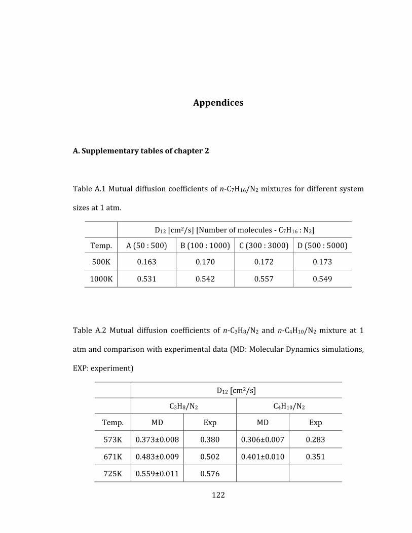
test the effect of system size on diffusion coefficients. Figure 2.3 and Table A.1 in the
Appendix A show computed mutual diffusion coefficients of normal heptane and
nitrogen (n-C7H16/N2) mixtures at 500 and 1000K. The error bars in Figure 2.3
represent standard deviations.
Figure 2.3 Mutual diffusion coefficients of n-C7H16/N2 mixtures at 1 atm for different
system sizes with error bars obtained from MD simulations.
.
Page 47
28
The maximum differences among the four mixtures are around 5% at the
both temperatures. When considering the error ranges, we can conclude that all of
the testing systems produced very similar diffusion coefficients. However, Figure 2.3
illustrates that system B (1100 molecules) has much larger statistical error
compared with that of system C (3300 molecules) or D (5500 molecules), especially
at high temperature (1000K). Although, system D showed slightly better results
than system C, we decided system C as the basis size for all our simulations due to
the compromise between the accuracy and computational cost.
2.3.2 The effect of concentration
In principle, mutual diffusion coefficients of ideal gas systems are
independent of relative concentration of each species. Therefore, the Chapman-
Enskog (C-E) equation (equation 2.1), derived from gas kinetic theory, does not
include any concentration dependent variables.
To evaluate the effect of concentration on diffusion, we analyzed 1%, 5%, and
10% mole fractions of n-C7H16 in the mixtures. We limited the mole fraction of
hydrocarbons at 10% because one of the main goals of this study is to compute
mutual diffusion coefficients for systems relevant to combustion applications. In
general combustion conditions, fuel concentrations for stoichiometric condition are
very low compared to those of nitrogen.
Table 2.2 shows mutual diffusion coefficients of n-C7H16/N2 mixture at
different concentration ratios. This result confirms that MD simulations also
Page 48
29
produce diffusion coefficients that are independent of the mole fractions of each
species in a low density gas, consistent with standard gas kinetic theory.
Table 2.2 Mutual diffusion coefficients of n-C7H16/N2 for different concentrations of
n-C7H16 (1%, 5%, and 10%) with MD simulations at 1atm.
D12 [cm2/s]
Temp. 1% 5% 10%
500K 0.172±0.006 0.173±0.007 0.172 ±0.005
1000K 0.564±0.017 0.558±0.013 0.557 ±0.012
2.3.3 Validity of atomistic force field for high temperature gas mixture
Since the OPLS AA potential parameters were optimized at normal boiling
temperature, direct application of this force field to different temperature
conditions cannot guarantee the accuracy of computed diffusion coefficients.
Therefore, comparison with available experimental data is needed to identify the
validity of the potentials under such conditions. However, only small amount of
experimental data are available for mutual diffusion coefficients of high
temperature gas systems especially for hydrocarbon/N2 mixtures. Consequently, we
chose n-C3H8/N2 and n-C4H10/N2 systems for our test simulations.
Page 49
30
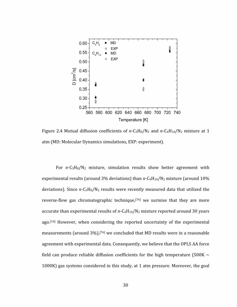
Figure 2.4 Mutual diffusion coefficients of n-C3H8/N2 and n-C4H10/N2 mixture at 1
atm (MD: Molecular Dynamics simulations, EXP: experiment).
For n-C3H8/N2 mixture, simulation results show better agreement with
experimental results (around 3% deviations) than n-C4H10/N2 mixture (around 10%
deviations). Since n-C3H8/N2 results were recently measured data that utilized the
reverse-flow gas chromatographic technique,[76] we surmise that they are more
accurate than experimental results of n-C4H10/N2 mixture reported around 30 years
ago.[16] However, when considering the reported uncertainty of the experimental
measurements (around 3%),[76] we concluded that MD results were in a reasonable
agreement with experimental data. Consequently, we believe that the OPLS AA force
field can produce reliable diffusion coefficients for the high temperature (500K ~
1000K) gas systems considered in this study, at 1 atm pressure. Moreover, the goal
Page 50
31
of this study is to identify the effect of molecular shapes on mass diffusion
coefficients and assess the validity of gas kinetic theory for polyatomic molecules
rather than compute exact diffusion values. Therefore, we concluded that the above
comparison demonstrated the validity of the use of the OPLS AA potentials for the
goal of this study. Further results of calculations are listed in Table A.2 in the
Appendix A.
2.4 Diffusion coefficients of heptane isomers
2.4.1 Configurations of heptane isomers
Although all-atom force field can describe molecular structures, we need to
clarify the effectiveness of these potentials in capturing the difference in the
configurations of molecules. For this purpose, we computed diffusion coefficients
for the mixtures of nitrogen and six heptane isomers. Since all isomers have the
same mass, deviations in computed diffusion coefficients among isomers originate
entirely from their structural differences. Moreover, the structural differences are
quite subtle so we expect that only a small amount of variance will manifest in final
diffusion values. Capturing these small discrepancies will verify the validity of our
approach to address the effect of molecular structures on mass diffusion coefficients.
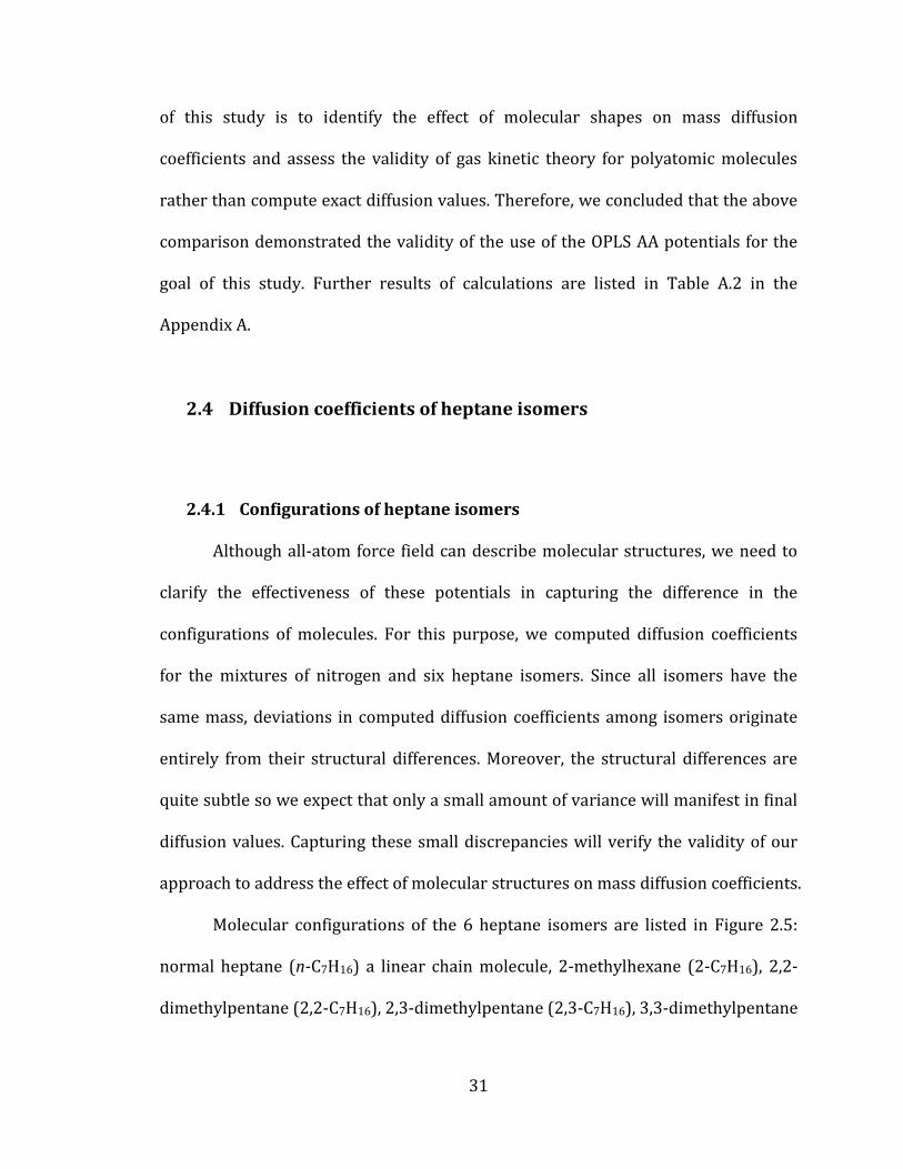
Molecular configurations of the 6 heptane isomers are listed in Figure 2.5:
normal heptane (n-C7H16) a linear chain molecule, 2-methylhexane (2-C7H16), 2,2-
dimethylpentane (2,2-C7H16), 2,3-dimethylpentane (2,3-C7H16), 3,3-dimethylpentane
Page 51
32
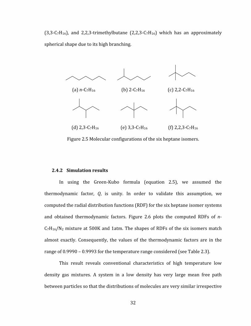
(3,3-C7H16), and 2,2,3-trimethylbutane (2,2,3-C7H16) which has an approximately
spherical shape due to its high branching.
(a) n-C7H16 (b) 2-C7H16 (c) 2,2-C7H16
(d) 2,3-C7H16 (e) 3,3-C7H16 (f) 2,2,3-C7H16
Figure 2.5 Molecular configurations of the six heptane isomers.
2.4.2 Simulation results
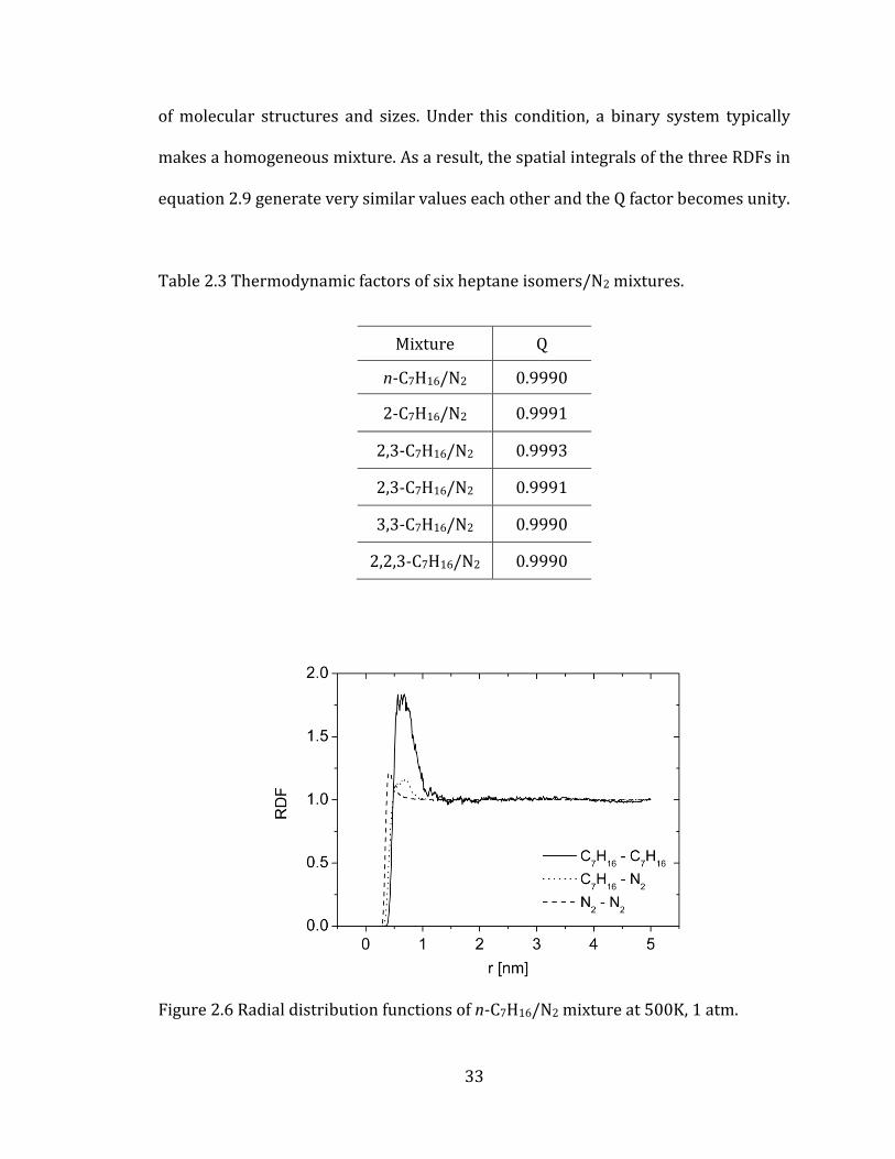
In using the Green-Kubo formula (equation 2.5), we assumed the
thermodynamic factor, Q, is unity. In order to validate this assumption, we
computed the radial distribution functions (RDF) for the six heptane isomer systems
and obtained thermodynamic factors. Figure 2.6 plots the computed RDFs of n-
C7H16/N2 mixture at 500K and 1atm. The shapes of RDFs of the six isomers match
almost exactly. Consequently, the values of the thermodynamic factors are in the
range of 0.9990 – 0.9993 for the temperature range considered (see Table 2.3).
This result reveals conventional characteristics of high temperature low
density gas mixtures. A system in a low density has very large mean free path
between particles so that the distributions of molecules are very similar irrespective
Page 52
33
of molecular structures and sizes. Under this condition, a binary system typically
makes a homogeneous mixture. As a result, the spatial integrals of the three RDFs in
equation 2.9 generate very similar values each other and the Q factor becomes unity.
Table 2.3 Thermodynamic factors of six heptane isomers/N2 mixtures.
Mixture Q
n-C7H16/N2 0.9990
2-C7H16/N2 0.9991
2,3-C7H16/N2 0.9993
2,3-C7H16/N2 0.9991
3,3-C7H16/N2 0.9990
2,2,3-C7H16/N2 0.9990
Figure 2.6 Radial distribution functions of n-C7H16/N2 mixture at 500K, 1 atm.
Page 53
34
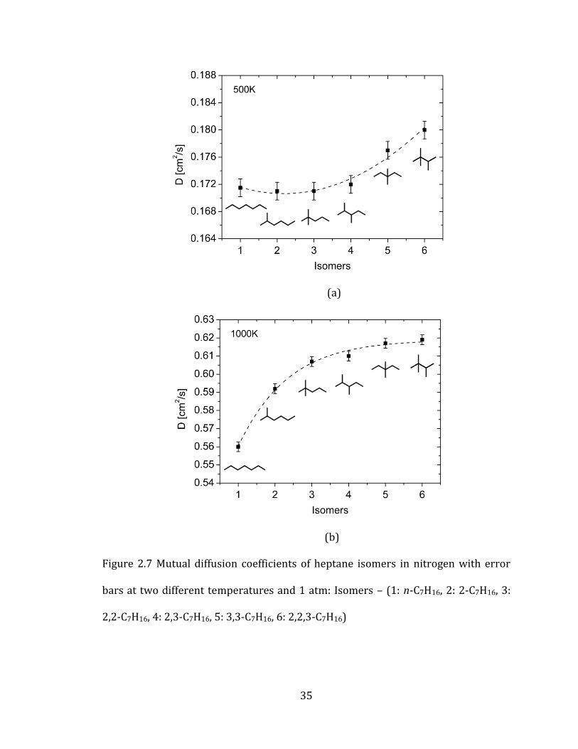
Figure 2.7 shows the distribution of diffusion coefficients of the isomers at
500K and 1000K. The differences in diffusion coefficients are small at low
temperature and increase with temperature. The results illustrate that as the
number of alkyl branches increases, the corresponding diffusion coefficients
increase. Experimental work on heptane isomers/helium mixtures also reported the
same trends of isomer diffusions. Eli Grushka et at.[77, 78] showed that heptane
isomers that have larger number of alkyl branches produced higher diffusion
coefficients. The consistency of these results justifies that our approach is able to
reproduce the experimental measurement correctly.
Page 54
35
(a)
(b)
Figure 2.7 Mutual diffusion coefficients of heptane isomers in nitrogen with error
bars at two different temperatures and 1 atm: Isomers – (1: n-C7H16, 2: 2-C7H16, 3:
2,2-C7H16, 4: 2,3-C7H16, 5: 3,3-C7H16, 6: 2,2,3-C7H16)
Page 55
36
The above results illustrate that the number of methyl branches and their
relative locations in a molecule changes the overall molecular configurations and
these structural variations affect diffusion values. To identify these effects, we
computed radius of gyrations (Rg) of heptane isomers and investigated the relation
between diffusion coefficients and molecular configurations. The radius of gyration
of a molecule describes the overall spread of atoms and represents their equilibrium
conformations. Therefore, it has been used as geometric factors for various
polyatomic molecules.[79-81] In this study, we computed the radius of gyrations from
the following relation:
3
1
Rg I
(2.17)
where Iαα denotes the moment of inertia of principal axes.
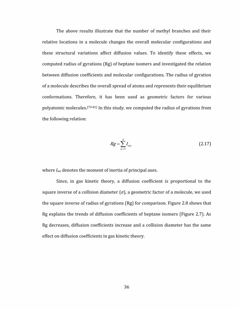
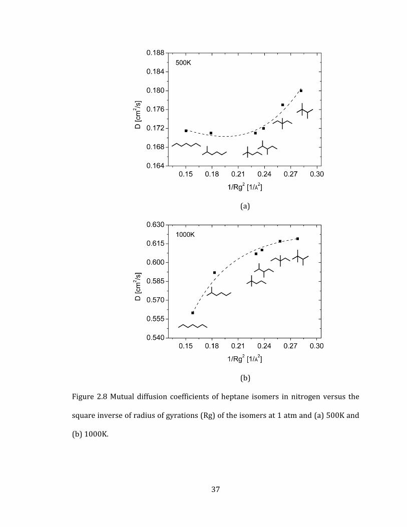
Since, in gas kinetic theory, a diffusion coefficient is proportional to the
square inverse of a collision diameter (σ), a geometric factor of a molecule, we used
the square inverse of radius of gyrations (Rg) for comparison. Figure 2.8 shows that
Rg explains the trends of diffusion coefficients of heptane isomers (Figure 2.7). As
Rg decreases, diffusion coefficients increase and a collision diameter has the same
effect on diffusion coefficients in gas kinetic theory.
Page 56
37
(a)
(b)
Figure 2.8 Mutual diffusion coefficients of heptane isomers in nitrogen versus the
square inverse of radius of gyrations (Rg) of the isomers at 1 atm and (a) 500K and
(b) 1000K.
Page 57
38
The above result implies that Rg can be related to a collision diameter and can be
used as a geometric factor that explains the trends of diffusion values. Figure 2.8
also reveals that as the number of methyl branches increases, the collision diameter
(or Rg) decreases and, consequently, a diffusion coefficient increases.
To address the temperature dependence of diffusion coefficients, we plotted
the results in the temperature range considered (See Figure 2.9). In Figure 2.9, only
three isomers are presented for clarity of the plot. Experimental measurement of
mutual diffusion coefficients for gas mixtures at 1 atm showed that measured values
had the following form[76, 82]
12nD AT (2.18)
where A and n are fitting constant and T is the temperature of the system. Therefore,
we will express diffusion coefficients in the same way by fitting our results with
equation 2.18 through least mean square fitting procedure.
The mixture of 2,2,3-C7H16/N2 has the highest mass diffusivities among
isomers in all temperature due to the smallest collision diameter (or Rg) and n-
C7H16/N2 has the lowest diffusion coefficients. More results about all other isomers
are listed in Table A.3 in the Appendix A.
Page 58
39
Figure 2.9 Mutual diffusion coefficients of three heptane isomers in nitrogen as a
function of temperature at 1 atm. Symbols: MD results; Curves: least mean square
curve fittings of MD results.
2.5 Diffusion coefficients of hydrocarbon molecules
In the previous section we verified our approaches to identify the effect of
molecular configurations on diffusion coefficients with heptane isomers. In this
section, we computed mutual diffusion coefficients of hydrocarbons in nitrogen
mixtures. Hydrocarbon classes considered in this study are linear alkanes,
cycloalkanes, and aromatic molecules, which typically constitute conventional
transportation fuels or fuel surrogates. For each mixture, the results of five
simulations were averaged in order to increase statistical accuracy of velocity
correlations.
Page 59
40
2.5.1 Linear alkanes
Linear alkanes are the most abundant constituents in conventional
hydrocarbon fuels and are typically employed as representative fuel components for
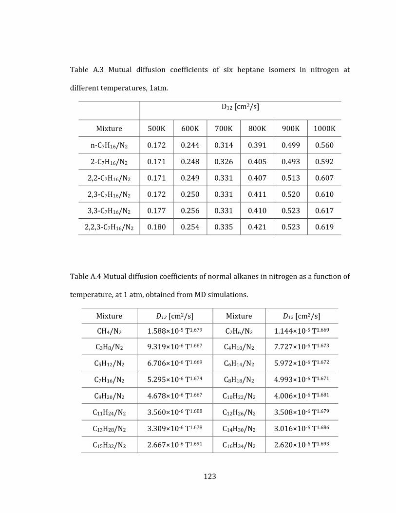
conventional combustion modeling. In this study, we selected sixteen linear alkanes
(from methane, CH4 to hexadecane, C16H34) to identify the effect of the length of
linear molecules on diffusion coefficients.
MD results are presented in Figure 2.10. As the number of methyl groups
increases, the diffusion coefficients decrease and the equation 2.18 successfully
describes the temperature dependency of diffusion coefficients. Detailed results of
all linear alkanes are listed in Table A.4 in the Appendix A.
Figure 2.10 Mutual diffusion coefficients of linear alkanes in nitrogen at 1 atm as a
function of temperature. The curves correspond to the least mean square curve
fittings of MD results.
Page 60
41
Figure 2.10 reveals that the difference in diffusion coefficients among mixtures
becomes larger as temperature increases. This trend implies that the difference in
diffusion coefficients of Figure 2.10 results from the coupling effect of mass,
molecular configuration, and temperature (T). Therefore, we removed the
temperature effect by dividing the computed diffusion coefficients by the factor of
T1.5 because diffusion coefficients are proportional to T1.5 in an ideal gas. This result
was plotted in Figure 2.11 and the curves show that the difference is diffusion
values are very similar irrespective of temperature. Since the mass of a molecule is
independent of temperature, we conclude that the effect of molecular configurations
on diffusion coefficients is almost independent of temperature for target systems.
Figure 2.11 Mutual diffusion coefficients of linear alkanes in nitrogen at 1 atm,
scaled with 1/T1.5 to remove the temperature effect.
Page 61
42
Another advantage of using MD simulations over gas kinetic theory to study
mass diffusion is the ability to determine the self diffusion coefficient of each
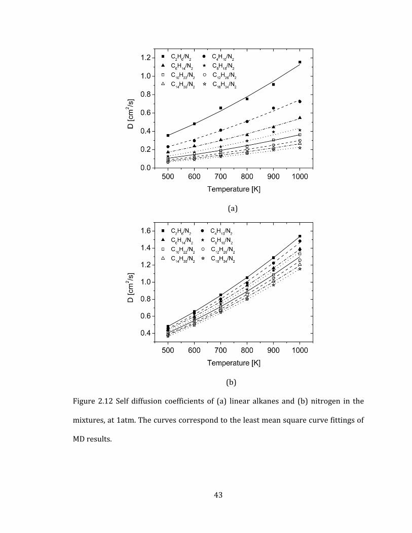
component in mixtures. Figure 2.12 reports the self-diffusion coefficients of normal
alkanes and nitrogens in each system. The results reveal that unlike nitrogen
(Figure 2.12 (b)), the diffusion coefficients of linear alkanes (Figure 2.12 (a)) show
significant variations among the studied systems.
Mutual diffusion coefficients are computed from the summation of two
velocity auto-correlation terms of each species and three velocity cross-correlation
terms (equation 2.5). Our results showed that the cross-correlation terms accounted
for negligible portions (less than 1%) of the diffusion values. Therefore, the mutual
diffusion coefficients depend on only self diffusion coefficients of two species and
their mole fractions (equation 2.19). Equation 2.19 also confirms that a species of
smaller mole fraction has a dominant effect on deciding diffusion coefficients. As a
result, the trends in self diffusion coefficients of linear alkanes (Figure 2.12 (a)) are
very similar to those of mutual diffusion coefficients (Figure 2.10).
12 nitrogen alkanes alkanes nitrogenD x D x D (2.19)
Page 62
43
(a)
(b)
Figure 2.12 Self diffusion coefficients of (a) linear alkanes and (b) nitrogen in the
mixtures, at 1atm. The curves correspond to the least mean square curve fittings of
MD results.
Page 63
44
2.5.2 Cycloalkanes
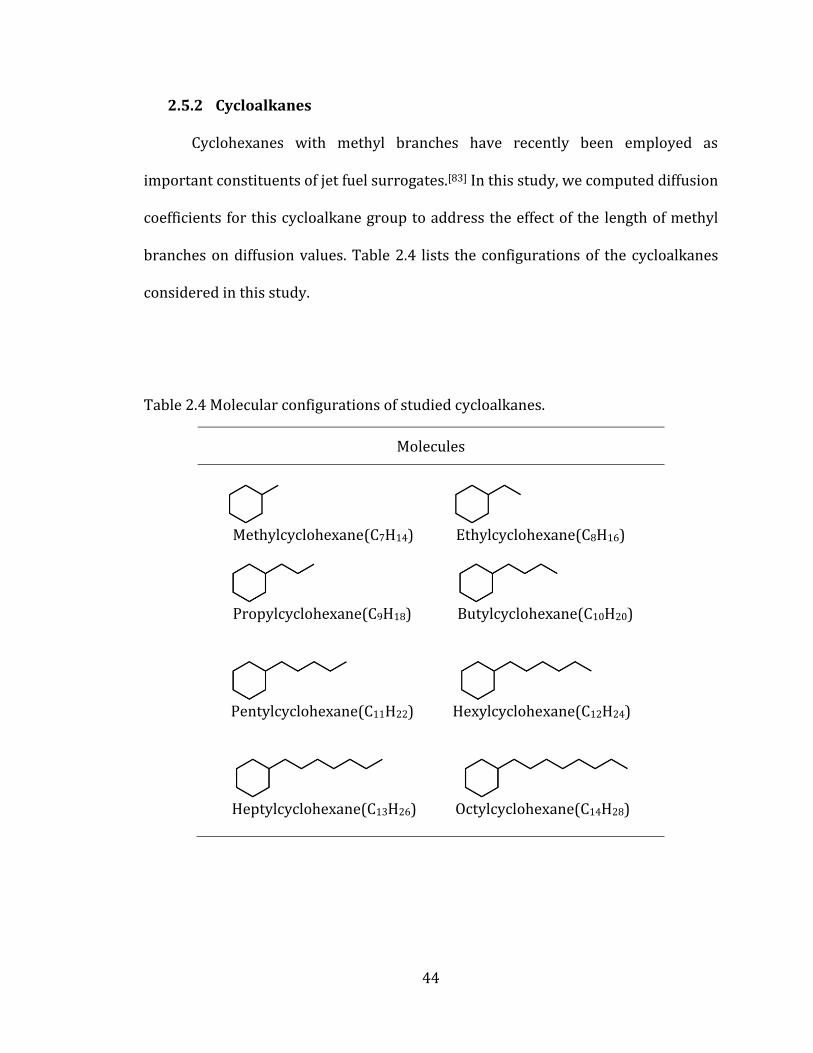
Cyclohexanes with methyl branches have recently been employed as
important constituents of jet fuel surrogates.[83] In this study, we computed diffusion
coefficients for this cycloalkane group to address the effect of the length of methyl
branches on diffusion values. Table 2.4 lists the configurations of the cycloalkanes
considered in this study.
Table 2.4 Molecular configurations of studied cycloalkanes.
Molecules
Methylcyclohexane(C7H14) Ethylcyclohexane(C8H16)
Propylcyclohexane(C9H18) Butylcyclohexane(C10H20)
Pentylcyclohexane(C11H22) Hexylcyclohexane(C12H24)
Heptylcyclohexane(C13H26) Octylcyclohexane(C14H28)
Page 64
45
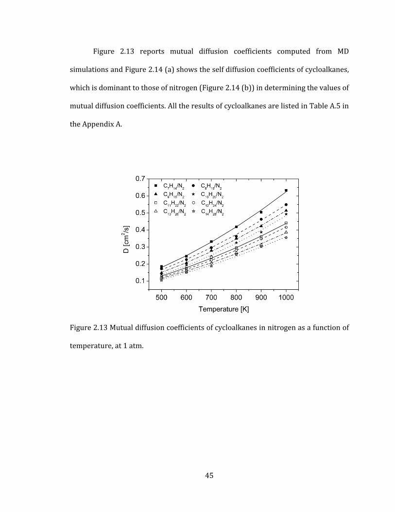
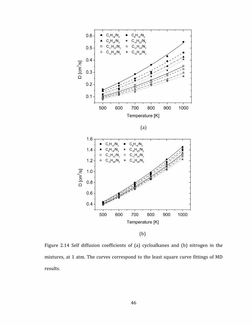
Figure 2.13 reports mutual diffusion coefficients computed from MD
simulations and Figure 2.14 (a) shows the self diffusion coefficients of cycloalkanes,
which is dominant to those of nitrogen (Figure 2.14 (b)) in determining the values of
mutual diffusion coefficients. All the results of cycloalkanes are listed in Table A.5 in
the Appendix A.
Figure 2.13 Mutual diffusion coefficients of cycloalkanes in nitrogen as a function of
temperature, at 1 atm.
Page 65
46
(a)
(b)
Figure 2.14 Self diffusion coefficients of (a) cycloalkanes and (b) nitrogen in the
mixtures, at 1 atm. The curves correspond to the least square curve fittings of MD
results.
Page 66
47
The above cycloalkane series has similarity in variation of their
configurations to those of linear alkanes. To show this trend, we compared the
change of diffusion coefficients as additional methyl groups are added sequentially
both to linear alkanes and to cyclohexanes (Figure 2.15). This result shows that the
contributions of an additional methyl group to diffusion coefficients for both groups
are very similar. The shift in the two curves is related to the presence of the six-
member aliphatic ring in cycloalkanes. The constrained arrangement of the aliphatic
ring has much smaller deformation than linear alkanes. As a result, cycloalkanes
have smaller effective area and consequently, produce higher diffusion coefficients.
Figure 2.15 Mutual diffusion coefficients of normal alkanes (C7H16 ~ C14H30) and
cycloalkanes (C7H14 ~ C14H28) in nitrogen, 1 atm. The curves correspond to the least
square curve fittings of MD results.
Page 67
48
2.5.3 Aromatic molecules
Aromatic hydrocarbons are usually regarded as important precursors for
soot formation.[84, 85] Moreover, benzene and naphthalene are frequently employed
as representative aromatic compounds in jet fuel surrogate blends.[5] In this study,
we computed mutual diffusion coefficients for polycyclic aromatic hydrocarbons
(PAH) in nitrogen, from one-ring to four-ring aromatic molecules (Table 2.5).
Page 68
49
Table 2.5 Molecular configurations of studied PAHs.
structure Molecules
One-ring Benzene (C6H6)
Two-ring Naphthalene (C10H8)
Three-ring Anthracene (C14H10-a) Phenanthrene (C14H10-b)
Four-ring
Pyrene (C16H10)
Naphthacene (C18H12-a) Benz[a]Anthracene(C18H12-b)
Chrysene (C18H12-c) Triphenylene (C18H12-d)
Page 69
50
The results show very similar trends to those of the other two hydrocarbon
groups reported in the previous sections. Aromatic molecules are the main cause of
the variations in the mutual diffusion coefficients. As the number of aromatic rings
increases, diffusion coefficients decrease. Figure 2.16 and 2.17 show mutual and self
diffusion coefficients of each species respectively. Results of all aromatic mixtures
are listed in Table A.6 in the Appendix A.
Figure 2.16 Mutual diffusion coefficients of aromatic molecules in nitrogen as a
function of temperature, at 1 atm. The curves correspond to the least mean square
curve fittings of MD results.
Page 70
51
(a)
(b)
Figure 2.17 Self diffusion coefficients of (a) aromatic molecules and (b) nitrogen in
the mixtures, at 1 atm. The curves correspond to the least mean square curve
fittings of MD results.
Page 71
52
In order to differentiate between the effect of molecular configurations and
mass, we analyzed the mutual diffusion coefficients of two groups of isomers (see
Figure 2.18). Between three ring species, C14H10-a mixture has lower diffusion
coefficients than C14H10-b mixture over the entire temperature range considered
with a difference around 5%.
Four ring aromatic molecules also show a very similar trend. Diffusion
coefficients decrease as aromatic rings are configured linearly. C18H12-a mixture has
the smallest diffusion coefficients due to this configuration. Around 8% difference in
diffusion values was observed between C18H12-a/N2 and C18H12-d/N2. Although
C18H12-b and C18H12-c mixtures show around 1% difference in their diffusion values,
this deviation is too small to confirm the effect of molecular configuration when we
consider the error range of our calculations. However, these two molecules
produced larger diffusion coefficients than that of C18H12-a and smaller values than
that of C18H12-d.
Page 72
53
(a)
(b)
Figure 2.18 Mutual diffusion coefficients of isomers of aromatic hydrocarbons in
nitrogen, at 1 atm (a) two ring aromatic molecules (b) four ring aromatic molecules.
Page 73
54
The diffusion coefficients of the above aromatic isomers can be characterized
by employing eccentricity (e) of molecules.[86] Eccentricity measures non-sphericity
of a molecule and zero value represents a perfect sphere. The values increase as
non-sphericity of molecules increase. In this study, we computed the eccentricity of
molecules from the moment of inertia tensor:
min min1 1( )/3avg xx yy zz
I Ie
I I I I
(2.20)
where Ixx, Iyy, and Izz denote the moment of inertia of principal axes and Imin
represents the minimum moment of inertia among the three main axes. Since
aromatic molecules have planar structures, eccentricity can express their molecular
configurations more effectively than radius of gyration used for heptane isomers.
Page 74
55
(a)
(b)
Figure 2.19 Mutual diffusion coefficients of aromatic isomers in nitrogen at 1000K, 1
atm versus their eccentricity of (a) two ring aromatics and (b) four ring aromatics.
Page 75
56
Figure 2.19 illustrates that the eccentricity of molecules can explain the
trends of diffusion coefficients of aromatic isomers. As the eccentricity increases, the
diffusion coefficients decrease. Moreover, from Figure 2.19 (b) we can confirm why
C18H12-b and C18H12-c have very similar diffusion coefficients. This result shows that
the assumption of spherical structures of gas kinetic theory is not appropriate
especially for molecules that have planar structures. Aromatic rings have the almost
same surface area irrespective of their arrangement and the deformations of their
configurations during the interactions with other species are very small when
compared with linear alkane molecules. Therefore, the isomers have very similar
collision diameters and consequently, employing spherical representation for these
molecules cannot express these structural characteristics effectively. Our results
show that molecules that have configurations closer to spheres produce higher
diffusion coefficients even though the collision diameters are very similar each other.
2.6 Comparison with gas kinetic theory
The Chapman-Enskog equation (equation 2.1) is advantageous in computing
mutual diffusions coefficients due to its simplicity. However, the lack of potential
parameters (collision diameter, σ, and energy well depth, ε) for molecules
significantly limits its application. These potential parameters, especially for
polyatomic molecules, are rarely available. Therefore, in this study, we employed
correlations of corresponding state theory to obtain potential parameters, which
were introduced in previous sections. Equations 2.2 through 2.4 were used for these
calculations, with thermodynamic parameters obtained from the NIST chemistry
Page 76
57
web data base. We compared results from MD simulations with those from C-E
equation to show the effect of molecular configurations on diffusion coefficients.
This comparison will show the deviation in diffusion values originated from the
utilization of monatomic spherical potentials.
2.6.1 Thermodynamic properties and potential parameters
Unfortunately, not all thermodynamic data are available for the
hydrocarbons, considered in this study. Therefore we only listed the available
thermodynamic data and the computed potential parameters in Table A.7 through
A.9 in the Appendix A.
2.6.2 Linear alkanes
Based on the potential parameters in Tables A.7 to A.9, diffusion coefficients
were computed with the C-E equation. Figure 2.20 and Table A.10 in the Appendix A
report mutual diffusion coefficients of linear alkanes as a function of temperature.
Page 77
58
Figure 2.20 Mutual diffusion coefficients of linear alkanes in nitrogen as a function
of temperature, at 1 atm obtained from the C-E equation.
As shown in Figure 2.20, the C-E equation produced very similar trends of
diffusion coefficients compared with MD simulations (see Figure 2.10). For a more
distinctive comparison, diffusion coefficients of four mixtures were plotted in Figure
2.21.
Page 78
59
(a) (b)
(c) (d)
Figure 2.21 Comparison of mutual diffusion coefficients of (a) C2H6/N2, (b) C6H14/N2,
(c) C12H26/N2, and (d) C16H34/N2, at 1 atm (MD: Molecular dynamics simulations, C-E:
the Chapman-Enskog equation).
For the C2H6/N2 mixture, the results from MD simulations and those from C-E
equation match well. Slight deviations can be found in high temperature region, but
the overall values show a good agreement. However, the results of the C16H34/N2
mixture show totally different trends and exhibit large differences in diffusion
values over the entire temperature region. The average deviation between the two
Page 79
60
approaches is around 17% of diffusion values and MD simulations produced smaller
diffusion coefficients than C-E equation. This result implies that the C-E equation
can produce similar diffusion coefficients to those of MD simulations, when target
molecules can be regarded as a sphere such as, CH4 and C2H6. In other words, using
single body interaction potentials is not appropriate for molecules that have non-
spherical structures.
2.6.3 Cycloalkanes
The cycloalkane group considered in this study also shows similar trends of
diffusion coefficients to those of alkane group. As the number of methyl groups
increases, the diffusion coefficients decrease. Figure 2.22 and Table A.11 in the
Appendix A show this trend clearly.
Figure 2.22 Mutual diffusion coefficients of cycloalkanes in nitrogen as a function of
temperature, at 1 atm obtained from the C-E equation.
Page 80
61
(a) (b)
Figure 2.23 Comparison of mutual diffusion coefficients of (a) C7H14/N2 and (b)
C14H28/N2, at 1 atm (MD: Molecular dynamics simulations, C-E: Chapman-Enskog
equation).
The C7H14/N2 mixture shows a 4% deviation between the two approaches
and the C14H28/N2 mixture reveals a much larger deviation, around 16% (see Figure
2.23). As in linear alkanes, the C-E equation presented larger diffusion coefficients
than MD simulations, likely due to the use of monatomic spherical potentials for
cycloalkanes.
2.6.4 Aromatic molecules
Figure 2.24 and Table A.12 in the Appendix A show mutual diffusion
coefficients of aromatic molecules in nitrogen computed from C-E equation. The
trends of diffusion coefficients are very similar to those of MD simulations.
Page 81
62
Figure 2.24 Mutual diffusion coefficients of aromatic molecules in nitrogen as a
function of temperature at 1 atm obtained from the C-E equation.
(a) (b)
Figure 2.25 Comparison of mutual diffusion coefficients of (a) C6H6/N2 and (b)
C18H12-a/N2, at 1 atm (MD: Molecular dynamics, C-E: Chapman-Enskog equation).
Page 82
63
The comparison with MD simulations (Figure 2.25) shows that, in the
C6H6/N2 mixture, MD and C-E results are perfectly matched. However, the C18H12-
a/N2 mixture exhibits approximately a 10% difference in diffusion coefficients. Even
in this case, the C-E equation also produced higher diffusion coefficients than MD
simulations over entire temperature ranges.
2.7 The effect of molecular configurations
The comparison between MD simulations and the C-E equation showed that
single-body spherical potentials produced higher diffusion coefficients than all-atom
potentials. Although, this analysis revealed the difference in diffusion values, the
effect of molecular configuration on diffusion coefficients cannot be determined
from those simple comparisons. We need to employ a geometric factor that can
represent molecular structures at equilibrium state of MD simulations. Moreover,
this factor has to be comparable to a collision diameter because the latter also is
related to the molecular structure in gas kinetic theory. For this purpose, we
computed radius of gyration (Rg) of each molecule with MD simulations. Since the
computed Rg expresses equilibrium configurations obtained by averaging all
possible conformations, it can represent the structural characteristics of all-atom
description of MD simulations. The Rg can represent molecular configurations
effectively because it reproduces the moment of inertia of the all atom molecules. As
we confirmed in the result of heptane isomers (see Figure 2.8), Rg can be related to
a collision diameter and be used as a geometric factor that explains the trends of
diffusion values.
Page 83
64
Before the use of Rg for the analysis, the temperature dependence of Rg
should be noted. We computed Rg of the studied molecules in the temperature
range of 500 – 1000K but the values did not vary significantly. Therefore, in the
following, we are going to use the average value in the above temperature range,
hence neglect the small temperature effect.
In gas kinetic theory, the changes of collision diameters (σ) and energy well
depths (ε) cause the variations in diffusion coefficients at fixed temperature and
pressure condition. However, since the square inverse of σ is proportional to
diffusion coefficients, σ has a dominant effect on determining diffusion values over
energy well depths. As shown in Table 2.6, 10% perturbation of σ causes around
11.3% deviation from the original diffusion values. On the other hand, the same
amount of perturbation of ε produces only 1.5% deviation. As a result, in order to
simplify the comparison we assumed that the contribution of energy well depths (ε)
to diffusion values is negligible, and σ causes all the variations in diffusion values.
Table 2.6 The contributions of collision diameter and energy well depth to diffusion
coefficients of n-C7H16/N2 mixture when 10% perturbation of σ and ε are exerted.
D12 [cm2/s]
Temperature [K] No perturbation perturbed σ Perturbed ε
500 0.185 0.164 0.182
1000 0.630 0.559 0.623
Deviation [%] 0 11.3 1.5
Page 84
65
2.7.1 Linear alkanes
As shown in Figure 2.26, collision diameters of linear alkanes (Table A.7 in
the Appendix A) used for the C-E equation were plotted with respect to their
average radius of gyrations (Table A.13 in the Appendix A). If the collision diameters
(σC-E) are linearly related to the radius of gyrations (Rg), the assumption of spherical
molecules in gas kinetic theory can represent polyatomic molecules successfully.
However, Figure 2.26 illustrates that the second order fitting shows better matching
with Rg. This second order fitting represents the deviation from sphericity of a
molecule.
Figure 2.26 Collision diameters (σC-E) of linear alkanes obtained from the C-E results
and relations with average radius of gyrations (Rg).
Page 85
66
To compare with the MD results, we obtained new collision diameters (σMD)
from the diffusion coefficients of MD simulations. Based on the discussion in the
previous section, we obtained σMD by inserting the ε values of Table A.7 in the
Appendix A into the C-E equation. These σMD represent new collision diameters that
should be used to reproduce the diffusion coefficients of all-atom MD simulations
with the same energy well depths employed for the C-E equation. In this way, we
can address the effect of molecular configurations on diffusion coefficients by using
single geometric parameters. The σMD of linear alkanes are listed in the Table A.14 in
the Appendix A and Figure 2.27 represents the first and second order fitting results
of σMD versus Rg. Although, we can still observe a little difference between the first
and second order fitting, the deviation is much smaller when compared with the C-E
results in Figure 2.26. This small discrepancy results from the temperature
dependence of the radius of gyration and the effect of energy well depths that we
neglected in our analysis. The smaller deviations in Figure 2.27 reveal that MD
simulations can take into account molecular structures more effectively in diffusion
calculations.
Page 86
67
Figure 2.27 New collision diameters (σMD) of linear alkanes obtained from MD
results and relations with average radius of gyrations (Rg).
Figure 2.28 Comparison of collision diameters of linear alkanes obtained from MD
and C-E results. Solid and dashed lines represent second-order fitting of σMD and σC-E
respectively.
Page 87
68
Figure 2.28 shows comparison between σMD and σC-E. The plot clearly
demonstrates that the C-E equation presents larger deviation as the number of
methyl groups increases. This trend implies that the C-E equation cannot produce
reliable diffusion coefficients for polyatomic molecules.
The relation between σMD and σC-E of linear alkanes can be obtained by
combining the two second order fitting expressions. In equation 2.21, the two
collision diameters are related with only Rg. This relation suggests a simple way
that can implement the effect of molecular configurations into the gas kinetic theory.
2
2
3.1115 1.4412 0.0465
3.1271 1.3203 0.0786MD C E
Rg Rg
Rg Rg
(2.21)
2.7.2 Cycloalkanes
The same comparison was conducted for cycloalkane group and the results
were plotted in Figure 2.29. The σMD of cycloalkanes are listed in Table A.15 in the
Appendix A. As in the results of linear alkanes, the C-E equation shows larger
deviation as the number of methyl groups increases. The fitting results show that
MD simulations can take into account the effect of molecular configurations
successfully when compared with the C-E equation.
Page 88
69
Figure 2.29 Comparison of collision diameters of cycloalkanes obtained from MD
and C-E results. Solid and dashed lines represent second-order fitting of σMD and σC-E
respectively.
The relation between σMD and σC-E of cycloalkanes is suggested in equation
2.22 and the Rg values are also listed in the Appendix A (Table A.16). New collision
diameters that include the effect of molecular structures can be obtained the
following relation.
2
2
3.7153 1.4779 0.0811
3.0126 1.8859 0.2042MD C E
Rg Rg
Rg Rg
(2.22)
Page 89
70
2.7.3 Aromatic molecules
We compared four mixtures (C6H6/N2, C10H8/N2, C14H10-a/N2, and C18H12-a)
to identify the effect of the number of rings in linearly configured aromatic
molecules. Figure 2.30 shows that the deviations between the two approaches
increase as the number of ring increases.
Figure 2.30 Comparison of collision diameters of linearly configured aromatic
molecules obtained from MD and C-E results. Solid and dashed lines represent
second-order fitting of σMD and σC-E respectively.
The relation between σMD and σC-E of linearly configured aromatic molecules
is presented in equation 2.23. As in the other hydrocarbon groups, Rg expresses the
Page 90
71
trends of collision diameters successfully. The σMD and Rg values of all aromatic
molecules considered studied are listed in the Appendix A (Table A.17 and A.18).
2
2
1.8895 2.4283 0.2037
2.9125 1.5972 0.0963MD C E
Rg Rg
Rg Rg
(2.23)
Figure 2.31 illustrates the results of four ring aromatic isomers. In this group,
we only plotted the σMD versus Rg. The results of the C-E equation are only available
for C18H12-a due to the lack of experimental thermodynamic properties for other
isomers.
As we mentioned in section 2.5, eccentricity (e) can explain the trends of
diffusions among isomers more effectively than radius of gyrations (Rg) due to their
planar structures. However, we used Rg for these isomers to assign a single
geometric factor for all hydrocarbon groups considered in this study. Moreover,
even though, C18H12-b and C18H12-c deviate from the fitting result, the difference in
diffusion coefficients between the two species is very small (see Figure 2.19).
Therefore, we concluded that the deviations of those two molecules exert very small
effect on providing reasonable relations between Rg and σMD.
Page 91
72
Figure 2.31 Comparison of collision diameters of four ring aromatic molecules
obtained from MD results. Solid represent second-order fitting of σMD.
The relation between σMD and σC-E of four ring aromatic isomers is presented
in equation 2.24. For this expression, we employed the value of C18H12-a as σC-E
because it is the only available data for the C-E equation.
210.2023 2.3456 0.4810
7.3871MD C E
Rg Rg
(2.24)
2.8 Conclusions
In this chapter, we computed mutual diffusion coefficients of three
hydrocarbon groups in nitrogen carrier gas by using both the Chapman-Enskog (C-E)
equation and Molecular Dynamics (MD) simulations. After qualitative comparison
Page 92
73
between the two approaches, we identified the effect of molecular configurations on
diffusion coefficients by employing radius of gyrations (Rg). Our results showed that
Rg could reproduce the trends of diffusion coefficients successfully and also could
be used as a geometric factor that expresses molecular configurations effectively.
We related Rg to the collision diameters obtained both from MD simulations (σMD)
and from the C-E equation (σC-E). In this process, we observed that σMD produced
much smaller deviations from the first order fitting with Rg. As a result, we
concluded that MD simulations could take into account molecular configurations
more effectively in diffusion calculations. The relations between σMD and σC-E are
also presented for each hydrocarbon groups to implement the effect of molecular
configuration into the C-E equation.
Page 93
74
Chapter 3
The equivalent single body potentials of polyatomic molecules
3.1 The effect of potentials on diffusion
In the previous chapter, we observed that molecular configurations exerted
influence on the diffusion coefficients and all-atom MD simulations are more
effective than gas kinetic theory in incorporating the effect of molecular structures
into diffusion calculations. These results also showed that all-atom potentials
produced smaller diffusion coefficients for all hydrocarbon classes compared with
monatomic spherical potentials. This discrepancy between the two approaches was
more distinctive for molecules that have higher mass and larger number of atoms.
However these differences are the consequences of a more detailed description of
molecular configurations and the employment of different potentials. In order to
evaluate the relative importance of these two contributions, we removed the effect
of the structures by reducing the all-atom multi body molecular potentials to
equivalent single body potentials. For this purpose in this chapter, we computed
Page 94
75
new Lennard-Jones (L-J) 12-6 potential parameters for the three hydrocarbon
groups that we studied in chapter 2 by using MD simulations and OPLS AA force
field. The new single body potential parameters were compared with the single
body potential parameters (Tables A.7 to A.9 in the Appendix A) used for the C-E
equation in the previous chapter.
3.2 Thermodynamic properties from MD simulations
Besides experimental measurements, the correlation of corresponding state
is the most widely used to estimate L-J potential parameters (σ and ε) for gas kinetic
theory.[48] Since this approach requires only critical temperature (Tc) and pressure
(Pc), and normal boiling temperature (Tb) of each species, the first step to obtain
new potential parameters by using MD simulations should be the computation of
the above thermodynamic properties.
To obtain the Tc, Pc, and Tb from MD simulations, we computed the chemical
potential at a given temperature and for different densities. This allowed us to
compute liquid – vapor coexistence curves, the saturated pressures and liquid and
vapor densities. From these liquid and vapor density values, we estimated the three
thermodynamic properties (Tc, Pc, and Tb).[87, 88]
Several approaches have been developed for the calculations of coexistence
curves such as the Gibbs Ensemble Monte Carlo (GEMC) technique[89], NPT test
particle method[90], and NVT test particle method.[91] The GEMC technique has been
widely used because the approach does not require many simulations for different
system sizes nor free energy calculations.[92-94] However, volume fluctuations limit
Page 95
76
stable simulations at high temperature region and the NPT test particle method also
has the same problem.[95] On the other hand, volumes are fixed during simulations
in the NVT test particle method so that this approach can perform stable simulations
in the temperature region close to the critical point. Therefore, we used this method
in this study.
In brief, we determined the coexistence curves and equilibrium vapor
pressure by computing chemical potentials for liquid and vapor states separately at
a constant temperature and volume condition. The pressure at the intersection of
liquid and vapor curves in the pressure versus chemical potential plane is the
equilibrium liquid – vapor pressure at a given temperature.[91] Pressures however,
can be determined in a straightforward way from MD simulations. On the other
hand, computing the chemical potentials requires a more complex approach.
3.2.1 Chemical potentials
The difficulty in computing chemical potential lies in measuring free energy.
Chemical potential of a constant volume (V) and constant temperature (T) system is
defined as:
, ,
i
i N V T
A
N
(3.1)
where A denotes the Helmholtz free energy of the system and N is the number of
molecules. Since the free energy is related to the canonical partition function itself
Page 96
77
rather than being an ensemble average of the partition function,[74] different
approaches are developed to circumvent this issue. A class of methods is based on
the coupling parameter approach.[96] In these techniques, the coupling parameters
are variables implemented into potentials to describe the continuous change of a
system from the initial state to the final state.[96] In other words, the Hamiltonian of
this transition can be written as:
1 0( ) (1 )H H H 0 1 (3.2)
where λ is the coupling parameter and H1 and H0 denote Hamiltonians at state λ=1
and λ=0 respectively.
Even though partition functions cannot be directly evaluated in a simulation,
their derivatives with respect to coupling parameters can be evaluated as an
ensemble average[74]:
, ,
( )exp ( )
( )
exp ( )
N
NN V T
UU drdA U
d U dr
(3.3)
where U is the potential energy of the system, expressed as a function of the
coupling parameter. The kinetic energy of the system does not need to be
considered because the kinetic energy is a quadratic function of momentum and its
contribution to microcanonical partition function is analytical.[97] Hence, we can
simply integrate out this term from the total partition function.
Page 97
78
The difference in free energy between two states and resulting chemical
potential are obtained by evaluating the following integrations (equations 3.4 and
3.5) with the slow growth method.[98]
1
0
( )( 1) ( 0)
UA A d
(3.4)
1
0
1 ( )i
i i
A Ud
N N
(3.5)
These integrations are related to a nonphysical path and the coupling parameters
connecting the fully coupled ( 0 ) and fully uncoupled ( 1 ) states. The system
has to change very slowly from fully coupled state to fully uncoupled state so that
the system remains equilibrated during the process. In order to obtain this gradual
change, discrete coupling parameters between 0 and 1 are chosen. The integration
over these parameters leads to the change of free energy.[99, 100] The number and
distribution of coupling values between 0 and 1 are related to the overlap of the
probability distributions of potential energy between the reference state and the
target state. Therefore, several intermediate states should be constructed so that the
overlap of the probability distributions of two consecutive states becomes sufficient
for direct evaluations.[97]
Page 98
79
3.2.2 Simulation method
The change of chemical potential was calculated from the potential energy
changes, ( )U
, of a system through removal of a molecule at a random position of
the system. For thermodynamic integration, we employed total eleven discrete
coupling parameters (λ= 0.0, 0.1, ···, 0.9, 1.0). At λ=0, a molecule fully interacts with
surrounding molecules and the molecule is fully uncoupled with a system at λ=1.
The potential energy interaction at each coupling value was computed with
linear interpolation between state 0 and 1. However, this approach causes
singularity problem when a molecule disappears (λ → 1) and in order to circumvent
this issue, soft core potential was used.[101]
0 10 1( ) (1 ) ( ) ( )scU r U r U r (3.6)
1
6 6 60 0
pr r (3.7)
1
6 6 61 1(1 )pr r (3.8)
where 0U and 1U denote normal potentials at state λ=0 and λ=1 respectively, α
is the parameter for soft core scaling and p is the soft core power, σ is the radius of
interactions and r is the distance between atoms.
In general, the value of ( )U
has a weak dependency on the choice of the
soft core scaling factor for λ → 1. However, the deviation at that point contributes
Page 99
80
only small portion to final result when the derivatives of potential energies are
integrated over all λ values. Therefore, we can neglect the effect of the parameters.
To test the convergence of simulations, we compared the results obtained
with simulations of different length for a box containing 300 octanes (n-C8H18). The
differences in free energy for 2, 3, and 4 ns runs were less than 2%. Therefore, we
chose 2ns simulation time for our calculations. Moreover, every system was pre-
equilibrated for 2ns before the actual simulations. All other conditions for
simulations are the same as those for diffusion calculations.
Figure 3.1 shows an example of free energy calculation of an octane system
at 540K and 42.7 kg/m3 density. The integration of these discrete potential energies
yields 1.756 KJ/mol for the free energy difference between the initial and the final
states. Subsequently, this value becomes the difference of chemical potential at a
given temperature and density.
Page 100
81
Figure 3.1 The change of potential energy of n-C8H18 as a function of coupling
parameters at 540K and 42.7 kg/m3 density.
The errors on Figure 3.1 were estimated by using block averaging method[102]
and an example of the error analysis for λ=0.5 was plotted in Figure 3.2. The dashed
line is the estimated error obtained by assuming all the blocks are independent. The
solid line is the fitted results by using the following exponential function:[103]
1 2
22 / /1 2
1 2
2( ) 1 1 (1 ) 1 1t tt e e
T t t
(3.9)
where σ, α, 1 , and 2 are fitting constants and T is total simulation time.
Page 101
82
Figure 3.2 Estimated error by using block averaging analysis for λ=0.5 of Figure 3.1.
The above graph demonstrates that the error value is well converged. The estimated
errors for all λ values are listed in Table B.1 in the Appendix B.
3.2.3 Equilibrium vapor pressure and densities
Figure 3.3 illustrates the computed chemical potentials and pressures of
liquid and vapor octane systems at 540K. Simulations were performed at several
different volumes for both liquid and vapor branches to obtain relations between
chemical potential and pressure at a fixed temperature. The solid squares denote
liquid state and the hollowed circles represent vapor state. The intersection of the
two lines provides equilibrium vapor pressure (Psat) at a given temperature. Once
the Psat is obtained, the liquid density (ρliq) and vapor density (ρvap) can be computed
from liquid and vapor branches in Figure 3.3 respectively. However, the estimation
Page 102
83
of critical properties and normal boiling temperature requires the ρliq and ρvap at Psat
obtained at two different temperatures. To reduce the statistical error, we repeated
the same procedure for three different temperatures and we averaged the results
obtained for all the pairwise combinations.
Figure 3.3 Chemical potential and pressure of octane (n-C8H18) computed from MD
simulations at 540K.
In Table 3.1, we list Psat, ρliq, and ρvap values both from MD simulations and
from experimental measurement for comparison. Experimental data were obtained
from NIST chemistry database.
Page 103
84
Table 3.1 Comparison of equilibrium vapor pressures (Psat), liquid densities (ρliq)
and vapor densities (ρvap) of linear alkanes at Psat and different temperatures. Dv
denotes the average percentile deviations from experimental values.
MD EXP
Temp
[K] Psat
[bar] ρliq
[kg/m3] ρvap
[kg/m3] Psat
[bar] ρliq
[kg/m3] ρvap
[kg/m3]
C2H6 290 33.4 226.5 52.3 35.2 351.7 77.4
280 27.1 237.2 42.2 28.1 383.2 56.6
270 21.4 245.8 33.9 22.1 407.8 42.3
Dv [%] 3.9 35.8 25.9
C4H10 400 22.4 263.1 45.9 24.9 408.5 73.1
390 19.2 273.5 40.2 20.9 433.2 57.5
380 15.9 281.5 34.1 17.4 454.2 45.8
Dv [%] 8.9 36.8 30.9
C6H14 470 15.5 301.1 37.2 17.2 444.4 59.3
460 13.1 311.6 32.4 14.6 463.8 48.2
450 11.0 320.8 27.9 12.3 481.1 39.4
Dv [%] 9.7 32.8 33.1
C8H18 550 17.6 286.8 55.6 19.1 389.7 92.2
540 15.5 309.6 48.4 16.5 419.6 72.6
530 13.0 327.5 42.1 14.3 443.2 58.7
Dv [%] 8.5 26.4 32.8
The results show that OPLS AA parameters underestimate equilibrium
pressures and densities. The average percentile deviation (Dv) of equilibrium
Page 104
85
pressure from experimental results is 3.9% for ethane (C2H6) and around 9% for
other normal alkanes, while MD simulations underestimate the densities around 30%
of all species. These results demonstrate the characteristics of OPLS AA potentials at
a temperature which differs substantially from the temperature used in the force
field derivation. This force field was optimized at normal boiling temperature and
liquid density was not tested at high temperature in their derivation process.[63]
Based on the above results, we expect that all equilibrium pressures and densities
obtained in this study are lower than measured values. We listed computed Psat, ρliq,
and ρvap of all hydrocarbon groups considered in this study in the Appendix B
(Tables B.2 to B.4)
3.2.4 Computed thermodynamic properties
With the computed ρliq and ρvap (Tables B.2 to B.4), critical temperature can
be estimated by using the following scaling law:[104]
1
( )2
liq vap cA T T (3.10)
where ρliq and ρvap denote liquid and vapor densities at Psat respectively, T is
temperature where ρliq and ρvap are computed, and β is estimated as 0.325[105, 106].
Fitting parameter, A, and critical temperature, Tc, are obtained at the same time by
inserting ρliq and ρvap of two different temperatures (T) into equation 3.10.
Page 105
86
Critical pressure, Pc, and normal boiling temperature, Tb, can be estimated by
using the following Clausius-Clapeyron equation:
expB
P CT
(3.11)
where B and C are fitting parameters, which can be estimated by inserting the Psat
and its corresponding temperature (T) into the equation 3.11. After these fitting
parameters are determined, we can obtain the Pc by substituting T of the equation
3.11 with Tc and can also compute Tb by substituting P with 1 atm.
In Tables B.5 to B.7 in the Appendix B, we list both the computed critical
properties and normal boiling temperatures and relevant experimental data for all
the hydrocarbons. The comparison reveals that critical properties and boiling
temperatures are in agreement with experimental data within a 7% deviation.
These deviations are significantly small when compared with those of the densities.
The reason for these results is that liquid-vapor coexistence curves are shifted
toward lower density region without significant changes in shapes. As a result,
critical properties and boiling temperatures have smaller deviation from
experimental results even though the densities are less accurately reproduced.
3.3 Equivalent single body potentials of all atom potentials
Once the thermodynamic properties (Tc, Pc, and Tb) were obtained, L-J 12-6
potential parameters can be computed by using the correlations of corresponding
Page 106
87
state (equations 2.2 to 2.4). The computed parameters for all the hydrocarbons are
listed in the Appendix B (Tables B.8 to Table 10).
3.4 Comparison with the C-E equation and MD simulations
Based on the equivalent potentials obtained in the previous section, we
computed diffusion coefficients of all the hydrocarbons by using the C-E equation.
The computed diffusion values were compared with both those of MD simulations
(Tables A.4 to A.6 in the Appendix A) and those of the C-E equation that used
potential parameters obtained from experimental data (Tables A.10 to A.12 in the
appendix) to show the difference in diffusion coefficients among those three
approaches. As done in the previous chapter, we also related collision diameters (σ)
to radius of gyration (Rg) and compared the results with those reported in the
chapter 2. These comparisons will reveal the relative contributions of the molecular
configuration and the employment of different potentials to diffusion coefficients.
3.4.1 Linear alkanes
Figure 3.4 illustrates the comparison of mutual diffusion coefficients of linear
alkanes mixtures obtained with three different approaches: MD simulations (MD),
the C-E equation with potential parameters obtained from experimental data (C-
EEXP), and the C-E equation with equivalent single body potential parameters
obtained from MD simulations in this chapter (C-EEquiv).
Page 107
88
As shown in Figure 3.4, the C-EEquiv produced very similar diffusion values to
those of the C-EEXP and has large deviation from MD results especially for long-chain
linear alkanes. It follows that the single body equivalent potentials cannot take into
account molecular configurations in diffusion calculations even though these
potentials are derived by using an all-atom potential. Moreover, this similarity
between C-EEXP and C-EEquiv proves that the deviations between MD simulations and
the C-EEXP, also analyzed in chapter 2, are caused by primarily the difference in
molecular configurations rather than the employment of different potentials.
Page 108
89
(a) (b)
(c) (d)
Figure 3.4 Comparison of mutual diffusion coefficients of (a) C2H6/N2, (b) C6H14/N2,
(c) C12H26/N2, and (d) C16H34/N2, at 1 atm (MD: Molecular dynamics, C-EEXP: C-E
equation with experiment data, and C-EEquiv: C-E equation with equivalent single
body potentials).
To investigate how much information on molecular configurations was
retained with this procedure, we computed collision diameters from the diffusion
coefficients of C-EEquiv (σEquiv) and compared with σC-E and σMD. As done in the
Page 109
90
previous chapter, σEquiv were computed by inserting the energy well depths (ε) of
Table A.7 in the Appendix A into the C-E equation (equation 2.1). Therefore, σEquiv
represents collision diameters that should be used to reproduce the diffusion
coefficients of the C-EEquiv with the same energy well depths employed for the C-EEXP.
Figure 3.5 illustrates that the σEquiv produces much larger deviation from the
linear relation with Rg when compared with that of MD. Moreover, the trends of the
σEquiv are very similar to those of σC-E and the deviations from σMD increase as the
number of methyl groups increases. This result also confirms that the equivalent
single body potentials and the correlations of corresponding state approaches
cannot yield reliable diffusion coefficients for polyatomic molecules.
Figure 3.5 Comparison of collision diameters of linear alkanes obtained from MD, C-
EEXP, and C-EEquiv results. Curves represent second-order fitting of σMD, σC-E, and
σEquiv respectively.
Page 110
91
3.4.2 Cycloalkanes
As before, the trends of diffusion obtained from C-EEquiv are very similar to
those of the C-EEXP and Figure 3.6 illustrates these results clearly. As the non-
sphericity of molecules increases (C14H28), the deviation between MD and C-EEquiv
increases. The similarity between C-EEXP and C-EEquiv is more evident as the shapes
of molecules deviate from sphere structures. Again, these trends indicate the
limitations of single body spherical potentials in computing diffusion coefficients of
polyatomic molecules.
(a) (b)
Figure 3.6 Comparison of mutual diffusion coefficients of (a) C7H14/N2 and (b)
C14H28/N2, at 1atm (MD: Molecular dynamics, C-EEXP: C-E equation with experiment
data, and C-EEquiv: C-E equation with equivalent single body potentials).
As shown in Figure 3.7, the collision diameters of C-EEquiv are also very
similar to those of C-EEXP. From the large deviation between MD and C-EEquiv, we can
Page 111
92
conclude that all-atom MD simulations are the most effective approach among those
three methods to compute diffusion coefficients of polyatomic molecules.
Figure 3.7 Comparison of collision diameters of cycloalkanes obtained from MD, C-
EEXP, and C-EEquiv results. Curves represent second-order fitting of σMD, σC-E, and
σEquiv respectively.
3.4.3 Aromatic molecules
Aromatic molecules also show similar results to those of the other two
hydrocarbon groups. Figure 3.8 illustrates mutual diffusion coefficients of four
aromatic molecules that have linearly configured structures. For C6H6/N2 mixture,
all of the approaches produced very similar diffusion coefficients. However, for
C18H12-a/N2 mixture, C-EEquiv shows large deviation from MD. This result is evidence
that single body spherical potentials are not appropriate in the diffusion
calculations of linearly configured multi-ring aromatic molecules.
Page 112
93
(a) (b) Figure 3.8 Comparison of mutual diffusion coefficients of (a) C6H6/N2 and (b)
C18H12-a/N2, at 1atm (MD: Molecular dynamics, C-EEXP: C-E equation with
experiment data, and C-EEquiv: C-E equation with equivalent single body potentials).
We can observe the limitation of this approach more clearly from the relation
between the radius of gyrations and the collision diameters of C-EEquiv. The
deviations between MD and the both C-E results increase as the number of aromatic
rings increase (Figure 3.9). This effect is likely the sum of both the single body
approximation and the employment of the force field far from its intended
temperature range.
For isomers, we did not find any noticeable difference in collision diameters
because the thermodynamic properties are very similar. In our simulations, the
simple change in the arrangement of aromatic rings does not affect the potentials
obtained from the correlations of corresponding state, showing another important
limitation of this approach.
Page 113
94
Figure 3.9 Comparison of collision diameters of aromatic molecules obtained from
MD, C-EEXP, and C-EEquiv results. Curves represent second-order fitting of σMD, σC-E,
and σEquiv respectively.
3.5 Conclusions
In this chapter, we obtained equivalent single body potentials for all the
studied hydrocarbons by reducing the multi body potentials. Free energy
calculations were conducted to identify the coexistence curves and the correlations
of corresponding state were used to obtain these equivalent L-J potential
parameters.
Diffusion coefficients computed with these equivalent potentials were very
similar to those from experimentally derived potentials and showed large
deviations from MD results. Based on this result, we conclude that the molecular
Page 114
95
configurations have a dominant effect on determining the deviations between MD
simulations and the C-E equation. The comparison of collision diameters also
revealed that single body spherical potentials cannot take into account molecular
configurations in diffusion calculations and cannot distinguish between isomers.
Therefore, among the three approaches that we compared, molecular dynamics
simulations with all-atom potentials provide the most effective way to compute
diffusion of various hydrocarbons studied in this work and the correlations of
corresponding state did not yield reliable diffusion coefficients for polyatomic
molecules.
Page 115
96
Chapter 4
Breakdown mechanisms of Decalin
4.1 Decalin
Decahydronaphthalene, also known as decalin (C10H18), is a bi-cyclic organic
compound of the naphthene class (Figure 4.1) and is the saturated analogue of
naphthalene. Decalin can occur in cis- and trans- conformations and the latter is
energetically more stable due to reduced steric interactions.[107, 108]
Figure 4.1 Trans-Decalin
Page 116
97
Decalin has been shown to be one of the most thermally stable and
endothermic fuel components of advanced jet fuels.[109, 110] In addition, it has shown
favorable combustion characteristics in both gas turbines and diesel engines.[111, 112]
Moreover, decalin can decompose without forming deposits so that it can be used at
high temperatures.[113] This is one of the critical characteristics required for an
advanced jet fuel.[114, 115] Decalin is also attractive as a potential hydrogen donor to
suppress pyrolytic deposits.[116, 117] By donating hydrogen atoms to radicals, which
are formed during the thermal decomposition process, decalin helps to prevent the
formation of various thermal deposits.
For these reasons, decalin has been employed as a reference component of multi-
ring naphthene classes for JP-8 surrogates.[5, 118, 119]
Surrogates with 35 % by volume of
decalin showed good agreement with experimental results on the sooting tendency of
pool fire.[120]
Agosta et. al. have included 6 % by volume of decalin in their surrogate to
match the auto-ignition behavior of hydrocarbon fuels.[118]
Despite of the importance of decalin for combustion research, the
fundamental reaction mechanisms of decalin have not been identified yet. Prompted
by this need, the analysis of the breakdown mechanisms of decalin was performed
by using Density Functional Theory (DFT) method. All transition states and
intermediate states were identified, along with possible reaction pathways. Reaction
rates were also computed for these reaction pathways. Finally, the identified
pathways were implemented in a kinetic mechanism analysis code to simulate the
pyrolysis environment.
Page 117
98
4.2 Computational method
4.2.1 Electronic structure calculations
We explored potential energy surface of each reaction pathway by using a
hybrid non local density functional theory (B3LYP), namely, Becke’s three-
parameter non local exchange[121, 122] with the non local correlation function of Lee,
Yang and Parr.[123] This level of theory has been found to be sufficiently accurate for
predicting the transition state properties for hydrogen abstraction reactions by
radicals.[124, 125] Therefore, the theory has been widely used to study hydrogen
abstraction reactions from hydrocarbons.[126-128] The geometry and frequency
calculations for all of the species were carried out using the 6-31G(d,p) basis set.
Transition States (TS) were identified by the existence of only a singular imaginary
frequency. The frequency calculations also allowed the zero-point energy (ZPE)
corrections to be obtained. Intrinsic Reaction Coordinate (IRC) calculations were
carried out to verify that each transition state connected the corresponding
reactants and products of a given reaction. All computations were carried out by
using the GAUSSIAN 03 package.[129]
4.2.2 Reaction rates
The Rice-Ramsperger-Kassel-Marcus (RRKM) theory and the canonical
Transition State Theory (TST) methods were used to derive high pressure limit rate
constants for unimolecular and bimolecular reactions, respectively.[130-132] To
Page 118
99
consider nonlinear Arrhenius effects, two parameter Arrhenius pre-exponential
factors, A and n, were incorporated in the form of ATn. Calculated rate constants for
each reaction as a function of temperature were fitted into the modified Arrhenius
form as:
( ) exp( / )nak T AT E RT (4.1)
Each rate constant was calculated by using the code TheRate (THEoretical
RATEs), from the web-based Computational Science and Engineering Online (CSE-
Online) environment.[133] Transmission coefficients, which account for the quantum
mechanical tunneling effect, were calculated by using the Eckart method.[134] The
thermal rate coefficient is expressed as:
††( )
( ) ( )( )
B
V
k TBR
k T Q Tk T T e
h T
(4.2)
where is the transmission coefficient, is the reaction symmetry number, †( )Q T
and ( )R T are the total partition functions per unit volume of the transition state
and reactant, respectively, †V is the classical barrier height, T is the temperature,
and Bk and h are the Boltzmann and Planck constant, respectively.
Page 119
100
4.3 Reaction pathways
Experimental results, previously reported for decalin pyrolysis at high
temperatures, have shown that the most probable initiation reactions of thermal
cracking are carbon-carbon (C9 – C10) bond cleavage (Figure 4.2 (a)) reaction and
hydrogen abstraction (from C1, C2 and C9) reactions (Figure 4.2 (b)).[135-137] Billaud
et. al. reported experimental results on the thermal cracking of decalin in a steam
pyrolysis environment.[138] However, detailed reaction pathways and their reaction
rate constants to build kinetic mechanisms are not yet available. Drawing on these
experimental observations, in this study, a series of new breakdown reaction
pathways of decalin were identified.
Page 120
101
(a)
(b)
Figure 4.2 Initiation reactions of decalin breakdown mechanisms: (a) carbon -
carbon bond cleavage, and (b) hydrogen abstractions.
4.3.1 Carbon – carbon bond cleavage reactions
Figure 4.3 shows the potential energy surface for the breakdown of decalin
through C9 – C10 bond cleavage reactions. No transition state was identified to
produce the intermediate ‘b’ (first order saddle point), and the reaction energy for ‘a
→ b’ is 88.02 kcal/mol. Further Carbon – Carbon (C – C) bond cleavage leads to the
formation of ‘c’ with an energy barrier of 38.11 kcal/mol.
Page 121
102
The addition of hydrogen to the bi-radical ‘c’ produces the intermediate ‘d’
without any transition barrier. Radical ‘d’ undergoes C – C bond scission and
produces C2H5 and ‘e’. The energy barrier for this step is 27.67 kcal/mol. Further C –
C bond scission leads to the formation of the C5H9 radical (f) and C3H5, followed by
the formation of the allyl radical (g) and ethylene.
Figure 4.3 Potential energy diagram starting from C9 - C10 bond cleavage reaction.
4.3.2 Hydrogen abstraction reactions
Figure 4.4 reports the initiation steps for the formation of 1-, 2- and 9-decalyl
radicals through hydrogen abstraction by CH3 radical. The energy barrier to
Page 122
103
produce 1-decalyl is 15.39 kcal/mol, higher than those of 2-decalyl and 9-decalyl,
which are 14.81 and 13.52 kcal/mol, respectively.
Figure 4.4 Energy barriers to produce 1-, 2-, and 9-decalyl radicals by hydrogen
abstraction reaction.
4.3.3 Reaction pathways from 1-decalyl radical
Nine pathways were identified for the subsequent reactions of 1-decalyl
radical (1b). Six of them (pathways 1 to 6) begin with the C8 – C9 bond scission and
the others (pathways 7 to 9) start with the C2 – C3 bond scission.
Figure 4.5 reports pathways 1 and 2 that form toluene (C7H8). The energy
barrier for the formation of radical ‘1c’ is 34.62 kcal/mol and the following
Page 123
104
hydrogen migration to produce ‘1d’ has a transition energy of 11.32 kcal/mol.
Subsequently, ‘1d’ decomposes to form ‘1e’ and the propyl (C3H7) radical. Hydrogen
abstraction from the intermediate ‘1e’ produces radical ‘1f’ with a transition energy
of 10.10 kcal/mol. From ‘1f’ two different pathways were identified that lead to the
formation of toluene. The ‘1f → 1g → 1h → toluene’ route involves hydrogen addition,
abstraction and further addition to produce toluene. From ‘1f’, the most significant
barrier is represented by ‘1f → 1g’, which is 31.21 kcal/mol.
In pathway 2, ‘1f’ undergoes two hydrogen abstraction reactions (‘1f → 2g’
and ‘2g → 2h’) and hydrogen addition (‘2h → toluene’) to produce toluene. The
energy barriers involved in this route are lower than the ones in pathway 1 and the
intermediates are very stable.
Page 124
105
Figure 4.5 Potential energy diagrams for pathways 1 and 2.
As shown in Figure 4.6, three reaction pathways (pathways 3 to 5) start from
the 1-decalyl radical (1b), which produce benzene and styrene. From the
intermediate ‘1c’, two subsequent β-scission reactions form ‘3d’ and ‘3e’. The energy
barriers of these reactions are 30.97 kcal/mol for ‘1c → 3d’ and 22.48 kcal/mol for
‘3d → 3e’. Sequential hydrogen abstraction reactions, ‘3e → 3f → 3g → benzene’, lead
to the formation of benzene.
Page 125
106
Figure 4.6 Potential energy diagrams for pathway 3, 4, and 5.
As an alternative, the species ‘3d’ can undergo hydrogen abstraction to form
the molecule ‘4e’. Styrene is then produced through hydrogen abstraction reactions,
according to the route ‘3d → 4e → 4f → 4g → 4h →styrene’. Decomposition of ‘4f’ into
‘3f’ and the vinyl radical (C2H3·) represents another pathway to form benzene
(pathway 5). The energy barrier for ‘4f → 3f’ is 35.56 kcal/mol, higher than that of
the ‘3d → 3e’ reaction, 22.48 kcal/mol. Benzene is then formed from ‘3f’ following
pathway 3 as previously described.
In Figure 4.7, pathway 6 that produces Ethylbenzene is illustrated.
Intermediate ‘3d’ undergoes hydrogen addition to produce ‘6e’ with an energy
Page 126
107
barrier of 20.92 kcal/mol energy. Subsequent hydrogen abstraction reactions
produce ethylbenzene through the pathway ‘6e → 6f → 6g → 6h → ethylbenzene’.
Figure 4.7 Potential energy diagram for pathway 6.
Pathways 7 and 8 that form benzene and styrene are illustrated in Figure 4.8.
Radical ‘1b’ undergoes C2 – C3 bond scission reaction to produce ‘7c’. This reaction
has an energy barrier of 35.37 kcal/mol, similar to that of the C8 – C9 bond scission
reaction of pathway 1, 34.62 kcal/mol. Two successive decomposition reactions first
produce ethylene and ‘7d’ and subsequently form the vinyl radical and ‘7e’. These
are the peculiar steps of this pathway. The energy barrier for ‘7c → 7d’ is 29.34
kcal/mol, which is very similar to that of reaction ‘1c → 3d’ of pathway 3, 30.97
Page 127
108
kcal/mol, but the ‘7d → 7e’ reaction shows a high energy barrier, 35.49 kcal/mol.
Subsequent hydrogen abstraction reactions produce benzene through the steps ‘7e
→ 7f → 7g → 3g → benzene’.
Pathway 8 proceeds from intermediate ‘7d’ through hydrogen abstraction
reactions to from styrene, through reactions ‘7d → 4e → 4f → 4g → 4h → styrene’.
Figure 4.8 Potential energy diagrams for pathways 7 and 8.
Figure 4.9 reports the last decomposition pathway for the 1-decalyl radical.
The ‘7c’ undergoes hydrogen addition and abstraction to produce ‘9e’. The energies
for reactions ‘7c → 9d’ and ‘9d → 9e’ are 22.46 kcal/mol and 14.75 kcal/mol,
respectively. The ‘9e’ decomposes to the vinyl radical and the species ‘9f’, which has
Page 128
109
a 34.88 kcal/mol energy barrier. Ethylbenzene is then produced through hydrogen
abstraction reactions.
Figure 4.9 Potential energy diagram for pathway 9.
All identified reaction pathways from the 1-decalyl radical start with carbon
– carbon bond scissions to open the ring structure. The products of these ring-
opening reactions undergo several elementary reactions to form mono-aromatic
molecules. Among these elementary reactions, hydrogen addition and migration are
the key steps. The presence of either of those two reactions determines the products
of their pathways. Benzene and styrene are obtained only from pathways that do
Page 129
110
not include any hydrogen addition or migration reactions (pathways 3, 4, 5, 7 and 8).
Conversely, hydrogen migration reactions are required to produce toluene
(pathways 1 and 2). Similarly, ethylbenzene is produced from the pathways that
include hydrogen addition reactions (pathways 6 and 9). These trends characterize
the breakdown mechanisms of multi-ring cycloalkanes when compared with those
of other hydrocarbon groups specifically, linear alkanes.
4.3.4 Reaction pathways from 2-decalyl radical
Two reaction pathways for the decomposition of the 2-decalyl radical are
reported in Figure 4.10. The sequence begins with C3 – C4 bond scission (‘10b → 10c’)
to form ‘10c’ and then undergoes hydrogen addition and abstraction to produce
‘10e’. An energy barrier of 17.81 kcal/mol is required to decompose ‘10e’ into ‘10f’
and the allyl radical (C3H5). Pathway 10 involves hydrogen abstraction reactions
that lead to the formation of toluene, through the route ‘10f → 10g → 10h →10i →
toluene’.
Page 130
111
Figure 4.10 Potential energy diagram for pathway 10.
In Figure 4.11, the ‘10b’ can produce ‘11c’ through C1 – C9 bond scission. The
energy barrier for this reaction, 34.64 kcal/mol, is slightly lower than that of ‘10b →
10c’, 37.47 kcal/mol. The ‘11c’ undergoes a decomposition reaction to produce C4H7
and the ‘7e’. From the ‘7e’, the pathway leads to the formation of benzene, analogous
to pathway 7.
Similar to the pathways of the 1-decalyl radical, benzene is produced from a
pathway which only consists of hydrogen abstraction and bond breaking reactions
(pathway 11). However, the pathway for toluene includes hydrogen addition
reactions right after C – C bond scission (pathway 10).
Page 131
112
Figure 4.11 Potential energy diagram for pathway 11.
4.3.5 Reaction pathways from 9-decalyl radical
Figure 4.12 shows reaction pathways for the 9-decalyl radical. The C1 – C2
bond scission reaction (12b → 12c) requires 34.04 kcal/mol of energy to overcome
the energy barrier and produce intermediate ‘12c’. This isomer radical (12c)
undergoes a decomposition reaction (12c → 12d) to form ‘12d’ and ethylene.
Successive hydrogen abstraction and addition reactions lead to the formation of
xylene.
Page 132
113
Figure 4.12 Potential energy diagram for pathway 12.
Alternatively, the ‘12c’ can undergo hydrogen addition (12c → 13d), 21.87
kcal/mol, and hydrogen abstraction (13d → 13e), 14.86 kcal/mol, to produce the
‘13e’. Propyl and the ‘1e’ are then formed from the decomposition of ‘13e’. From ‘1e’,
toluene is produced following the same reaction route described in pathways 1 and
2 (Figure 4.13).
The 9-decalyl radical produced xylene and toluene, and all of those pathways
involve hydrogen addition reactions. From the reaction pathways of three decalyl
radicals, we observed distinct features of the breakdown mechanisms of multi-ring
cycloalkanes to form mono-aromatic ring molecules. As we showed, all decalyl
radicals begin their breakdown with C – C bond scissions to open their aliphatic
Page 133
114
rings. Subsequently based on their resultant structures, those radicals follow
different pathways. Therefore obtaining accurate energy barriers of these ring
opening reactions is critical in order to correctly identify reaction pathways of
cycloalkane molecules. Another feature is the existence of hydrogen addition or
hydrogen migration determines the aromatic products of their pathways. Benzene
and styrene are produced only from the sequence of hydrogen abstractions and C –
C bond breaking reactions. Most of toluene is obtained from the pathways that
include a hydrogen migration reaction. The other products (ethylbenzene and
xylene) contain hydrogen addition reactions in their pathways.
Figure 4.13 Potential energy diagram for pathways 13 and 14.
Page 134
115
4.4 Kinetic modeling
Reaction rate constants were obtained at different temperature condition by
using the RRKM and TST methods. Computed high-pressure limit constants are
listed in Tables C.1 to C.13 in the Appendix C. The resulting thermal rate constants
are of reasonable accuracy as long as the high-pressure limit can adequately
describe the target reaction conditions. For flame modeling at ambient pressure, the
high-pressure limit approximation is generally valid, and therefore our computed
rate constants can be used in detailed kinetic modeling of atmospheric combustion.
The newly identified reaction pathways for decalin breakdown and their
relative reaction rates were implemented in a kinetic mechanism analysis code. The
CHEMKIN software package[139, 140] was utilized to study the time-dependent
chemical kinetics behavior of a closed homogeneous gas mixture system in the
temperature range of 700K – 1500K and 1 atm. The mechanism includes all the
reaction steps previously described. Table C.14 in the Appendix C reports the
calculated product yields (%) of benzene, toluene, styrene, ethylbenzene and xylene
as a function of temperature.
At low temperature conditions (700K), the major reaction product is
benzene, which is formed mainly through pathways 3, 7 and 11. The pathway 11
accounts for most of the benzene production within the temperature ranges
considered. At 700K, pathway 11 contributes 99% of benzene production and the
value goes down to 76% at 1500K. The contribution of pathways 3 and 7 to benzene
formation increases with temperature, reaching 8.55% and 14.69% at 1500K,
respectively.
Page 135
116
Toluene is produced through pathways 1 and 2. The other three routes
leading to toluene, pathways 10, 13 and 14 are less significant. Pathways 13 and 14
compete with pathway 12 to form xylene and pathway 10 overcomes Path 11 to
produce benzene. At low temperatures toluene is mainly formed through pathway 2
(99%). As the temperature increases the contribution of pathway 2 become less
significant. As a result, pathway 1 contributes 67% and pathway 2 does 32% to the
final yields of toluene at 1500K.
Benzene production reaches a minimum at 1000K, where the toluene yield
peaks. The amounts formed of both of these two compounds are interdependent, as
a result of the competition of pathways 1 and 7, in which the ‘1b’ can form ‘1c’ or ‘7c’
to produce toluene or benzene, respectively.
Styrene is produced through pathway 8 and the overall yield is low
compared with benzene and toluene. This result is due to the competition with
pathways 3 and 7 that lead to the formation of benzene.
Ethylbenzene is formed through pathways 6 and 9. At low temperatures,
pathway 9 represents the main production route for ethylbenzene. However at
1500K, pathway 6 accounts for 10% of the total yield. In the same way as styrene,
ethylbenzene accounts for very small portion of products due to the competition
with pathways 3 and 7.
Xylene is produced through pathway 12 and its yield increases as the
temperature goes up. Its production, however, is below 1% in the temperature
range analyzed.
Page 136
117
The overall results demonstrate that hydrogen abstraction and C – C bond
breaking reactions are energetically favorable than hydrogen abstraction and
hydrogen migration reactions. These trends explain the preferential formation of
benzene from the breakdown mechanisms of decalin.
4.5 Conclusions
Fourteen reaction pathways that connect decalin to five mono-aromatic
species (benzene, toluene, styrene, ethylbenzene and xylene) were identified. The
basic reactions for the new routes are carbon – carbon bond scission, dissociation,
hydrogen abstraction and hydrogen addition. Reaction rate constant for each
elementary reaction was computed and kinetic modeling analysis was also
conducted to evaluate the relative importance of each pathway. The computed
reaction pathways and their reaction rates can supply accurate kinetic data for
combustion modeling under conditions where high pressure limit rates are
applicable. Computed rate constants of decalin can be further incorporated in
existing kinetic mechanisms for flame combustion and pyrolysis analysis to improve
the prediction of aromatic concentrations.
Page 137
118
Chapter 5
Conclusions
This study aimed at investigating molecular transport and chemical kinetic
data of the components of jet fuel surrogates to improve the predictive capability of
their combustion reaction mechanisms. We used molecular modeling approaches to
compute and validate transport properties of various classes of hydrocarbons and
employed ab-initio techniques to identify the breakdown mechanisms of decalin, a
multi-ring cycloalkane component of fuel surrogates.
For molecular transport data, we first tested the validity of gas kinetic theory
for polyatomic molecules. One major assumption in gas kinetic theory is the
simplification of molecular configurations to spherical structures, which is
potentially problematic for large polyatomic molecules. To understand the effect of
this assumption, we compared gas kinetic theory with all-atom Molecular Dynamics
simulations. Since atomistic level modeling treats all bonded and non-bonded
interactions between atoms, it can be used to assess the effect of molecular
Page 138
119
structures on transport properties. Therefore, we computed mutual mass diffusion
coefficients of three hydrocarbon classes (linear alkanes, cycloalkanes and aromatic
molecules) in nitrogen carrier gas using both MD simulations and the analytical
equation of gas kinetic theory (Chapman-Enskog equation). This comparison reveals
that the Chapman-Enskog (C-E) equation overestimates diffusion coefficients of the
hydrocarbons considered in this study and the discrepancy increases as the
molecules become non-spherical.
To better understand these results, we measured the effect of molecular
configurations on mass diffusion coefficients by employing the radius of gyration
(Rg). Since Rg reproduces the moment of inertia of the molecules, it is one of the
simplest ways to represent vibrational and rotational information present in all-
atom MD simulations. To measure the contribution of molecular structures to
diffusion values, we related the computed Rg to the collision diameters obtained
both from MD simulations (σMD) and from the C-E equation (σC-E). In this procedure,
we observed that σC-E cannot be linearly related to the Rg. On the other hand, σMD
produced much smaller deviations from the linear relation with Rg for all
hydrocarbons. These results highlight the ability of MD simulations to take into
account differences in molecular configurations and that the C-E equation cannot
yield reliable diffusion coefficients especially for large molecules that have non-
spherical structures.
To assess the relative importance on diffusion coefficients of molecular
configurations with respect to the employed force field, we parameterized an
equivalent single body potential from the multi body all atom force field. Free
Page 139
120
energy calculations were conducted to identify the coexistence curves of systems in
the liquid – gas transition region. From these data, we estimated the new potentials
by using the correlations of corresponding state. Diffusion coefficients computed
with these equivalent potentials were very similar to those from the C-E equation
and showed large deviations from all-atom MD results. This comparison shows that
although the equivalent spherical potentials were derived from the all-atom MD,
thermodynamic properties cannot compensate for the lack of structural information.
This also confirms that the assumption of spherical molecules in gas kinetic theory
is not appropriate for polyatomic molecules and the molecular configurations have a
dominant effect on transport properties. With our approach however, we were able
to find a simple relation between molecular configuration and diffusion, relating Rg
and collision diameters (σMD and σC-E) for all the hydrocarbons. Hence we removed
the limitations of the C-E equation by including the effect of molecular
configurations.
The importance of this study lays not only in the improvement of existing
data and methods but also in the fact that it suggests a simple general approach to
deal correctly with new fuel components. Since standard gas kinetic theory and
experiments can hardly give reliable or enough data for all the molecules that are of
interest in hydrocarbon combustion or alternative fuels, accurate transport
properties should be obtained through other methods. All-atom MD simulations can
provide a simple and effective approach to overcome the above limitations and
obtain diffusion coefficients for new realistic fuel components.
Page 140
121
In the field of kinetic reactivity, we identified the breakdown mechanisms of
decalin, a bi-cyclic naphthene commonly employed as a representative component
of jet fuel surrogate. From ab-initio calculations, we obtained a total of fifteen
possible reaction pathways that connect decalin to five mono-aromatic species
(benzene, toluene, styrene, ethylbenzene and xylene). These reaction pathways are
initiated by two elementary reactions, carbon bond cleavage reaction or hydrogen
abstraction reactions. Each pathway connects the reactants to the products through
a series of about ten reaction steps chosen among four elementary reactions
(carbon bonds breaking reactions, dissociation reaction, hydrogen abstraction
reactions, and hydrogen addition reaction). Electronic structures and energy states
of all reactants, products, intermediates and transition states were explored for all
the identified pathways. The activation energy of each reaction step and the
geometry of all species were computed by using a hybrid density functional theory
(B3LYP) and 6-31G(d,p) basis set.
From these data, we computed rate constants for the unimolecular and
bimolecular reactions by using transition state theories in the temperature range of
700 – 1500K. The kinetic mechanism analysis shows the relative importance of each
reaction pathways and concludes that benzene and toluene comprise around 99% in
the product mixture. Computed rate constants of decalin can be further
incorporated in existing kinetic mechanisms for flame combustion and pyrolysis
analysis to improve the prediction of aromatic concentrations. Moreover, these
findings can be used to understand the chemical reactions of cycloalkanes as a
component of jet fuel surrogate.
Page 141
122
Appendices
A. Supplementary tables of chapter 2
Table A.1 Mutual diffusion coefficients of n-C7H16/N2 mixtures for different system
sizes at 1 atm.
D12 [cm2/s] [Number of molecules - C7H16 : N2]
Temp. A (50 : 500) B (100 : 1000) C (300 : 3000) D (500 : 5000)
500K 0.163 0.170 0.172 0.173
1000K 0.531 0.542 0.557 0.549
Table A.2 Mutual diffusion coefficients of n-C3H8/N2 and n-C4H10/N2 mixture at 1
atm and comparison with experimental data (MD: Molecular Dynamics simulations,
EXP: experiment)
D12 [cm2/s]
C3H8/N2 C4H10/N2
Temp. MD Exp MD Exp
573K 0.373±0.008 0.380 0.306±0.007 0.283
671K 0.483±0.009 0.502 0.401±0.010 0.351
725K 0.559±0.011 0.576
Page 142
123
Table A.3 Mutual diffusion coefficients of six heptane isomers in nitrogen at
different temperatures, 1atm.
D12 [cm2/s]
Mixture 500K 600K 700K 800K 900K 1000K
n-C7H16/N2 0.172 0.244 0.314 0.391 0.499 0.560
2-C7H16/N2 0.171 0.248 0.326 0.405 0.493 0.592
2,2-C7H16/N2 0.171 0.249 0.331 0.407 0.513 0.607
2,3-C7H16/N2 0.172 0.250 0.331 0.411 0.520 0.610
3,3-C7H16/N2 0.177 0.256 0.331 0.410 0.523 0.617
2,2,3-C7H16/N2 0.180 0.254 0.335 0.421 0.523 0.619
Table A.4 Mutual diffusion coefficients of normal alkanes in nitrogen as a function of
temperature, at 1 atm, obtained from MD simulations.
Mixture D12 [cm2/s] Mixture D12 [cm2/s]
CH4/N2 1.588×10⁻⁵ T1.679 C2H6/N2 1.144×10⁻⁵ T1.669
C3H8/N2 9.319×10⁻⁶ T1.667 C4H10/N2 7.727×10⁻⁶ T1.673
C5H12/N2 6.706×10⁻⁶ T1.669 C6H14/N2 5.972×10⁻⁶ T1.672
C7H16/N2 5.295×10⁻⁶ T1.674 C8H18/N2 4.993×10⁻⁶ T1.671
C9H20/N2 4.678×10⁻⁶ T1.667 C10H22/N2 4.006×10⁻⁶ T1.681
C11H24/N2 3.560×10⁻⁶ T1.688 C12H26/N2 3.508×10⁻⁶ T1.679
C13H28/N2 3.309×10⁻⁶ T1.678 C14H30/N2 3.016×10⁻⁶ T1.686
C15H32/N2 2.667×10⁻⁶ T1.691 C16H34/N2 2.620×10⁻⁶ T1.693
Page 143
124
Table A.5 Mutual diffusion coefficients of cycloalkanes in nitrogen as a function of
temperature, at 1 atm, obtained from MD simulations.
Mixture D12 [cm2/s] Mixture D12 [cm2/s]
C7H14/N2 2.695×10⁻⁶ T1.7882 C11H22/N2 1.852×10⁻⁶ T1.7924
C8H16/N2 2.492×10⁻⁶ T1.7823 C12H24/N2 1.764×10⁻⁶ T1.7919
C9H18/N2 2.239×10⁻⁶ T1.7874 C13H26/N2 1.611×10⁻⁶ T1.7938
C10H20/N2 2.041×10⁻⁶ T1.7911 C14H28/N2 1.520×10⁻⁶ T1.7931
Table A.6 Mutual diffusion coefficients of aromatic molecules in nitrogen as a
function of temperature, at 1 atm, obtained from MD simulations.
Mixture D12 [cm2/s] Mixture D12 [cm2/s]
C6H6/N2 3.599×10⁻⁶ T1.7829 C16H10/N2 1.744×10⁻⁶ T1.7953
C10H8/N2 2.539×10⁻⁶ T1.7835 C18H12-a/N2 1.501×10⁻⁶ T1.7966
C14H10-a/N2 1.902×10⁻⁶ T1.7914 C18H12-b/N2 1.592×10⁻⁶ T1.7944
C14H10-b/N2 1.961×10⁻⁶ T1.7937 C18H12-c/N2 1.572×10⁻⁶ T1.7941
C18H12-d/N2 1.652×10⁻⁶ T1.7937
Page 144
125
Table A.7 Thermodynamic properties and derived potential parameters of linear
alkanes
Molecules Tc [K] Pc [atm] Tb [K] σ [Å] ε/kB [K]
CH4 190.6 45.49 111.0 3.793 153.0
C2H6 305.3 48.35 184.6 4.274 266.2
C3H8 369.9 41.94 231.0 4.737 335.2
C4H10 425.0 37.50 273.0 5.102 400.8
C5H12 469.8 33.15 309.2 5.454 457.2
C6H14 507.6 29.80 341.9 5.747 511.5
C7H16 540.0 27.04 371.5 6.004 563.3
C8H18 568.9 24.57 398.7 6.256 611.4
C9H20 595.0 22.69 423.8 6.466 658.2
C10H22 617.8 20.82 447.2 6.680 703.2
C11H24 639.0 19.54 468.0 6.855 743.1
C12H26 658.2 17.76 489.0 7.096 782.6
C13H28 676.0 16.77 507.0 7.256 817.8
C14H30 693.0 15.79 523.0 7.455 841.7
C15H32 708.0 14.80 540.0 7.619 877.5
C16H34 722.0 13.83 554.0 7.841 895.8
Page 145
126
Table A.8 Thermodynamic properties and derived potential parameters of
cycloalkanes
Molecules Tc [K] Pc [atm] Tb [K] σ [Å] ε/kB [K]
C7H14 573.0 34.34 374.0 5.777 550.6
C8H16 609.0 30.00 405.0 6.144 594.1
C9H18 639.2 27.73 429.0 6.403 626.4
C10H20 667.1 25.36 453.0 6.675 659.6
C11H22 683.3 23.11 472.1 6.899 691.8
C12H24 700.2 21.36 493.8 7.065 737.5
C13H26 715.2 19.84 514.4 7.206 785.2
C14H28 728.6 18.52 534.1 7.321 836.1
Table A.9 Thermodynamic properties and derived potential parameters of aromatic
molecules
Molecules Tc [K] Pc [atm] Tb [K] σ [Å] ε/kB [K]
C6H6 562 48.25 353.1 5.144 531.9
C10H8 748 40.46 490.0 5.907 753.5
C14H10-a 873 28.62 613.0 6.764 983.5
C14H10-b 869 28.62 609.2 6.764 974.0
C16H10 936 25.75 667.9 7.119 1079.3
C18H12-a 987 23.58 716.2 7.387 1174.9
Page 146
127
Table A.10 Mutual diffusion coefficients of linear alkanes in nitrogen as a function of
temperature at 1 atm, obtained from the C-E equation.
Mixture D12 [cm2/s] Mixture D12 [cm2/s]
CH4/N2 1.483×10⁻⁵ T1.6923 C2H6/N2 8.982×10⁻⁶ T1.7139
C3H8/N2 6.668×10⁻⁶ T1.7252 C4H10/N2 5.354×10⁻⁶ T1.7349
C5H12/N2 4.469×10⁻⁶ T1.7429 C6H14/N2 3.844×10⁻⁶ T1.7504
C7H16/N2 3.376×10⁻⁶ T1.7573 C8H18/N2 3.001×10⁻⁶ T1.7636
C9H20/N2 2.716×10⁻⁶ T1.7692 C10H22/N2 2.471×10⁻⁶ T1.7743
C11H24/N2 2.285×10⁻⁶ T1.7788 C12H26/N2 2.082×10⁻⁶ T1.7839
C13H28/N2 1.949×10⁻⁶ T1.7876 C14H30/N2 2.083×10⁻⁶ T1.7839
C15H32/N2 1.723×10⁻⁶ T1.7934 C16H34/N2 1.833×10⁻⁶ T1.7900
Table A.11 Mutual diffusion coefficients of cycloalkanes in nitrogen as a function of
temperature at 1atm, obtained from the C-E equation.
Mixture D12 [cm2/s] Mixture D12 [cm2/s]
C7H14/N2 3.604×10⁻⁶ T1.7554 C11H22/N2 2.377×10⁻⁶ T1.7732
C8H16/N2 3.137×10⁻⁶ T1.7611 C12H24/N2 2.190×10⁻⁶ T1.7786
C9H18/N2 2.844×10⁻⁶ T1.7653 C13H26/N2 2.028×10⁻⁶ T1.7839
C10H20/N2 2.585×10⁻⁶ T1.7692 C14H28/N2 1.888×10⁻⁶ T1.7896
Page 147
128
Table A.12 Mutual diffusion coefficients of aromatic molecules in nitrogen as a
function of temperature at 1 atm, obtained from the C-E equation.
Mixture D12 [cm2/s]
C6H6/N2 4.347×10⁻⁶ T1.7530
C10H8/N2 2.782×10⁻⁶ T1.7799
C14H10-a/N2 1.866×10⁻⁶ T1.8043
C14H10-b/N2 1.877×10⁻⁶ T1.8036
C16H10/N2 1.600×10⁻⁶ T1.8139
C18H12-a/N2 1.413×10⁻⁶ T1.8221
Table A.13 Average radius of gyrations linear alkanes obtained with MD simulations.
Species Rg [Å] Species Rg [Å]
CH4 0.549 C2H6 0.978
C3H8 1.299 C4H10 1.617
C5H12 1.932 C6H14 2.244
C7H16 2.541 C8H18 2.845
C9H20 3.134 C10H22 3.421
C11H24 3.693 C12H26 3.951
C13H28 4.228 C14H30 4.484
C15H32 4.730 C16H34 4.978
Page 148
129
Table A.14 New collision diameters (σMD) of linear alkanes.
Species σMD [Å] Species σMD [Å]
CH4 3.849 C2H6 4.481
C3H8 4.935 C4H10 5.288
C5H12 5.821 C6H14 6.094
C7H16 6.517 C8H18 6.812
C9H20 7.147 C10H22 7.441
C11H24 7.747 C12H26 8.081
C13H28 8.427 C14H30 8.598
C15H32 8.973 C16H34 9.099
Table A.15 New collision diameters (σMD) of cycloalkanes.
Species σMD [Å] Species σMD [Å]
C7H14 6.135 C11H22 7.516
C8H16 6.545 C12H24 7.736
C9H18 6.859 C13H26 8.059
C10H20 7.187 C14H28 8.350
Page 149
130
Table A.16 Average radius of gyrations of cycloalkanes obtained with MD
simulations.
Species Rg [Å] Species Rg [Å]
C7H14 1.856 C11H22 3.084
C8H16 2.129 C12H24 3.391
C9H18 2.446 C13H26 3.695
C10H20 2.765 C14H28 3.988
Table A.17 New collision diameters (σMD) of aromatic molecules.
Species σMD [Å] Species σMD [Å]
C6H6 5.110 C18H12-a 7.991
C10H8 6.279 C18H12-b 7.708
C14H10-a 7.158 C18H12-c 7.803
C14H10-b 6.858 C18H12-d 7.534
C16H10 7.297
Table A.18 Average radius of gyrations of aromatic molecules obtained with MD
simulations.
Species Rg [Å] Species Rg [Å]
C6H6 1.528 C18H12-a 3.586
C10H8 2.196 C18H12-b 3.402
C14H10-a 2.883 C18H12-c 3.333
C14H10-b 2.744 C18H12-d 3.082
C16H10 2.778
Page 150
131
B. Supplementary tables of chapter 3
Table B.1 Estimated errors for all λ of Figure 3.1.
λ ( )U
[KJ/mol] Error [KJ/mol]
0.0 3.074 0.260
0.1 2.849 0.223
0.2 2.669 0.175
0.3 2.411 0.160
0.4 2.168 0.136
0.5 2.032 0.168
0.6 1.645 0.145
0.7 1.325 0.142
0.8 0.886 0.176
0.9 0.199 0.242
1.0 -0.331 0.242
Integration 1.756
Page 151
132
Table B.2 Equilibrium vapor pressure (Psat), liquid (ρliq) and vapor densities (ρvap) of
linear alkanes obtained from MD simulations.
CH4 C2H6
Temp [K] 150 160 170 270 280 290
Psat [bar] 9.7 15.4 22.5 21.4 27.1 33.4
ρliq [kg/m3] 222.7 214.9 206.2 245.8 237.2 226.5
ρvap [kg/m3] 13.9 22.3 33.2 33.9 42.2 52.3
C3H8 C4H10
Temp [K] 330 340 350 380 390 400
Psat [bar] 18.4 22.5 27.2 15.9 19.2 22.3
ρliq [kg/m3] 271.7 263.7 252.5 281.5 273.5 263.1
ρvap [kg/m3] 33.9 42.7 51.4 34.1 40.2 45.9
C5H12 C6H14
Temp [K] 420 430 440 450 460 470
Psat [bar] 13.6 16.3 19.1 11.0 13.1 15.5
ρliq [kg/m3] 303.5 294.3 282.9 320.9 311.6 301.1
ρvap [kg/m3] 33.5 39.5 45.5 27.9 32.4 37.2
C7H16 C8H18
Temp [K] 500 510 520 530 540 550
Psat [bar] 13.7 16.2 18.5 13.0 15.1 17.6
ρliq [kg/m3] 300.2 290.3 276.0 327.5 309.6 286.8
ρvap [kg/m3] 39.9 48.8 56.9 42.1 48.4 55.6
Page 152
133
C9H20 C10H22
Temp [K] 540 550 560 560 570 580
Psat [bar] 9.4 10.9 12.3 8.2 9.6 11.5
ρliq [kg/m3] 326.4 317.6 305.9 274.0 266.8 259.9
ρvap [kg/m3] 31.3 37.0 41.7 30.1 35.7 43.4
C11H24 C12H26
Temp [K] 580 590 600 610 620 630
Psat [bar] 7.4 8.8 10.0 8.4 9.9 11.2
ρliq [kg/m3] 299.1 292.2 283.3 301.1 292.9 280.9
ρvap [kg/m3] 27.5 33.1 38.1 33.6 40.5 45.8
C13H28 C14H30
Temp [K] 630 640 650 650 660 670
Psat [bar] 8.1 9.2 10.5 8.0 9.3 10.7
ρliq [kg/m3] 286.7 278.0 268.4 286.2 275.0 260.4
ρvap [kg/m3] 33.4 38.4 44.2 35.1 40.9 46.6
C15H32 C16H34
Temp [K] 650 660 670 670 680 690
Psat [bar] 6.0 7.1 8.0 6.2 7.1 8.1
ρliq [kg/m3] 293.4 286.9 278.1 298.3 289.3 277.7
ρvap [kg/m3] 26.0 31.7 36.2 28.6 34.3 39.3
Page 153
134
Table B.3 Equilibrium vapor pressure (Psat), liquid (ρliq) and vapor densities (ρvap) of
cycloalkanes obtained from MD simulations.
C7H14 C8H16
Temp [K] 530 540 550 560 570 580
Psat [bar] 17.0 20.1 22.7 15.0 17.1 19.0
ρliq [kg/m3] 354.7 341.8 322.9 369.5 356.3 339.7
ρvap [kg/m3] 46.3 54.2 59.8 42.9 47.9 52.3
C9H18 C10H20
Temp [K] 590 600 610 620 630 640
Psat [bar] 14.3 16.1 17.9 13.9 15.7 17.4
ρliq [kg/m3] 336.1 325.3 313.2 349.5 336.5 321.1
ρvap [kg/m3] 44.1 48.6 53.8 45.6 50.3 55.4
C11H22 C12H24
Temp [K] 630 640 650 650 660 670
Psat [bar] 10.5 12.2 13.5 8.7 10.4 11.7
ρliq [kg/m3] 350.7 342.5 331.1 364.8 351.9 338.7
ρvap [kg/m3] 35.9 41.7 45.7 34.1 37.0 41.6
C13H26 C14H28
Temp [K] 660 670 680 670 680 690
Psat [bar] 8.1 9.3 10.5 7.7 8.9 10.1
ρliq [kg/m3] 367.9 356.5 343.2 347.9 339.2 328.7
ρvap [kg/m3] 31.2 35.6 39.7 31.7 36.6 41.0
Page 154
135
Table B.4 Equilibrium vapor pressure (Psat), liquid (ρliq) and vapor densities (ρvap) of
aromatic molecules obtained from MD simulations.
C6H6 C10H8
Temp [K] 520 530 540 700 710 720
Psat [bar] 26.8 29.9 34.2 22.5 24.2 26.7
ρliq [kg/m3] 455.9 432.5 406.1 458.9 440.1 420.9
ρvap [kg/m3] 56.5 61.5 69.1 57.5 60.4 65.9
C14H10-a C14H10-b
Temp [K] 830 840 850 830 840 850
Psat [bar] 16.7 18.5 20.3 16.6 18.5 20.2
ρliq [kg/m3] 489.6 471.1 449.1 488.9 471.1 450.2
ρvap [kg/m3] 50.1 55.1 59.7 50.0 55.1 59.6
C16H10 C18H12-a
Temp [K] 890 900 910 910 920 930
Psat [bar] 14.9 16.5 18.2 10.7 11.7 12.9
ρliq [kg/m3] 478.6 459.8 437.4 501.6 486.9 471.5
ρvap [kg/m3] 46.8 51.7 56.0 36.0 39.6 43.9
C18H12-b C18H12-c
Temp [K] 910 920 930 910 920 930
Psat [bar] 10.9 11.8 13.0 10.8 11.7 13.0
ρliq [kg/m3] 500.7 487.4 472.3 501.8 487.2 471.8
ρvap [kg/m3] 35.9 39.5 44.0 36.0 39.7 44.0
C18H12-d
Temp [K] 910 920 930
Psat [bar] 10.8 11.8 12.9
ρliq [kg/m3] 501.2 486.8 472.1
ρvap [kg/m3] 35.8 39.5 43.8
Page 155
136
Table B.5 Critical pressures (Pc), critical temperatures (Tc) and normal boiling
temperatures (Tb) of linear alkanes. MD denotes Molecular Dynamics simulations
and EXP represents experimental data.
MD EXP
Tc [K] Pc [atm] Tb [K] Tc [K] Pc [atm] Tb [K]
CH4 195.5 47.0 112.4 190.6 46.0 111.7
C2H6 314.2 47.9 171.1 305.3 48.7 184.5
C3H8 379.6 40.8 228.2 369.8 42.5 231.1
C4H10 440.6 38.1 262.7 425.1 37.9 272.6
C5H12 482.4 32.9 304.7 469.7 33.7 309.2
C6H14 530.2 30.7 334.3 507.6 30.3 341.9
C7H16 548.6 26.0 364.1 540.2 27.4 371.6
C8H18 572.5 23.6 405.5 568.7 24.9 398.8
C9H20 609.4 22.2 424.9 594.6 22.9 423.9
C10H22 626.0 19.1 451.2 617.7 21.1 447.3
C11H24 654.3 18.9 465.3 639.0 19.5 469.1
C12H26 668.4 17.4 475.9 658.0 18.2 489.5
C13H28 694.5 16.9 501.7 675.0 16.8 508.6
C14H30 701.1 15.0 526.5 693.0 15.7 526.7
C15H32 725.5 14.1 544.4 708.0 14.8 543.8
C16H34 733.4 13.5 557.7 723.0 14.0 560.1
Page 156
137
Table B.6 Critical pressures (Pc), critical temperatures (Tc) and normal boiling
temperatures (Tb) of cycloalkanes. MD denotes Molecular Dynamics simulations and
EXP represents experimental data.
MD EXP
Tc [K] Pc [atm] Tb [K] Tc [K] Pc [atm] Tb [K]
C7H14 581.7 32.3 374.4 573.0 34.3 374.0
C8H16 621.6 28.2 390.4 609.0 30.0 405.0
C9H18 655.5 27.6 422.1 639.2 27.7 429.0
C10H20 679.0 25.7 451.9 667.0 25.4 453.0
C11H22 707.1 22.8 466.8
C12H24 721.3 20.5 512.7
C13H26 733.5 18.5 527.7
C14H28 749.2 17.6 526.7
Page 157
138
Table B.7 Critical pressures (Pc), critical temperatures (Tc) and normal boiling
temperatures (Tb) of aromatic molecules. MD denotes Molecular Dynamics
simulations and EXP represents experimental data.
MD EXP
Tc [K] Pc [atm] Tb [K] Tc [K] Pc [atm] Tb [K]
C6H6 569.1 47.9 361.3 562.0 48.3 353.1
C10H8 763.5 38.9 489.5 748.0 40.5 490.0
C14H10-a 894.2 30.8 622.8 873.0 28.6 613.0
C14H10-b 894.8 30.8 622.1 869.0 28.6 609.2
C16H10 953.4 26.8 687.0 936.0 25.8 667.9
C18H12-a 996.7 24.0 731.2 987.0 23.6 716.2
C18H12-b 995.8 23.8 730.6
C18H12-c 996.3 24.0 730.8
C18H12-d 996.2 24.0 730.5
Page 158
139
Table B.8 L-J 12-6 potential parameters for linear alkanes obtained from MD
simulations.
σ [Å] ε/kB [K]
CH4 3.771 154.9
C2H6 4.515 227.9
C3H8 4.915 315.6
C4H10 5.314 356.3
C5H12 5.648 425.2
C6H14 5.993 457.1
C7H16 6.288 513.6
C8H18 6.311 629.8
C9H20 6.637 649.6
C10H22 6.997 681.2
C11H24 7.184 685.0
C12H26 7.482 688.9
C13H28 7.591 738.1
C14H30 7.719 820.1
C15H32 7.884 840.2
C16H34 8.064 869.9
Page 159
140
Table B.9 L-J 12-6 potential parameters for cycloalkanes obtained from MD
simulations.
σ [Å] ε/kB [K]
C7H14 5.997 532.6
C8H16 6.417 540.7
C9H18 6.629 578.7
C10H20 6.766 638.6
C11H22 7.142 666.3
C12H24 7.197 770.7
C13H26 7.520 774.9
C14H28 7.725 779.2
Table B.10 L-J 12-6 potential parameters for aromatic molecules obtained from MD
simulations.
σ [Å] ε/kB [K]
C6H6 5.149 550.9
C10H8 6.115 724.5
C14H10-a 6.667 1001.2
C14H10-b 6.678 999.4
C16H10 6.966 1149.0
C18H12-a 7.256 1240.2
C18H12-b 7.277 1237.7
C18H12-c 7.257 1239.4
C18H12-d 7.255 1238.8
Page 160
141
C. Supplementary tables of chapter 4
Tables C.1 to C.14 list reaction rates constants.
F denotes forward reaction and R represents reverse reaction, Ea [kcal/mol] is the
activation energy of each reaction.
Arrhenius format, k(T) = ATn exp(-Ea/RT),
Table C.1 The reaction rate constants of pathway 1.
Page 161
142
Table C.2 The reaction rate constants of pathway 2.
Table C.3 The reaction rate constants of pathway 3.
Page 162
143
Table C.4 The reaction rate constants of pathway 4.
Table C.5 The reaction rate constants of pathway 5.
Page 163
144
Table C.6 The reaction rate constants of pathway 6.
Page 164
145
Table C.7 The reaction rate constants of pathway 7.
Table C.8 The reaction rate constants of pathway 8.
Page 165
146
Table C.9 The reaction rate constants of pathway 9.
Page 166
147
Table C.10 The reaction rate constants of pathway 10.
Page 167
148
Table C.11 The reaction rate constants of pathway 11.
Page 168
149
Table C.12 The reaction rate constants of pathway 12.
Page 169
150
Table C.13 The reaction rate constants of pathway 13.
Page 170
151
Table C.14 Calculated product yields (%) of benzene, toluene, styrene, ethylbenzene,
and xylene as a function of temperature
Page 171
152
References
[1] A. T. Holley, Y. Dong, M. G. Andac, F. N. Egolfopoulos, T. Edwards Proc. Combust.
Inst. 2007, 31, 1205-1213.
[2] J. A. Cooke, M. Bellucci, M. D. Smooke, A. Gomez, A. Violi, T. Faravelli, E. Ranzi
Proc. Combust. Inst. 2005, 30, 439-446.
[3] T. Edwards, L. Q. Maurice Journal of Propulsion and Power. 2001, 17, 461-466.
[4] J. T. Farrell, N. P. Cernansky, F. L. Dryer, D. G. Friend, H. C. A., C. K. LAw, R. M.
McDavid, M. C. J., A. K. Patel, H. Pitsch SAE international. 2007.
[5] A. Violi, S. Yan, E. G. Eddings, F. Sarofim, S. Granata, T. Faravelli, E. Ranzi
Combustion Science and Technology. 2002, 174, 399-417.
[6] M. Colket, T. Edwards, S. Williams, N. P. Cemansky, D. L. Miller, F. Egolfopoulos, P.
Lindstedt, K. Seshadri, F. L. Dryer, C. K. LAw, D. Friend, D. B. Lenhert, H. Pitsch, A.
Sarofim, M. Smooke, W. Tsang 45th AIAA Aerospace Science Meeting. 2007, AIAA-
2007-0770.
[7] A. T. Ingemarsson, J. R. Pedersen, J. O. Olsson Journal of Physical Chemistry A.
1999, 103, 8222-8230.
Page 172
153
[8] H. R. Zhang, E. G. Eddings, A. F. Sarofim, C. K. Westbrook Energy & Fuels. 2007, 21,
1967-1976.
[9] V. Calemma, S. Peratello, F. Stroppa, R. Giardino, C. Perego Industrial &
Engineering Chemistry Research. 2004, 43, 934-940.
[10] W. Vincenti, C. H. J. Kruger Introduction to physical gas dynamics. 1975.
[11] J. Millat, J. H. Dymond, C. A. N. d. Castro, Transport Properties of Fluids: Their
correlation, prediction and estimation, Cambridge university press, 1996.
[12] K. K. Kuo, Principles of Combustion, John Wiley & Sons, 1986.
[13] S. R. Turns, An Introduction to Combustion: Concepts and Applications,
McGraw-Hill, 2000.
[14] B. J. Alder, D. M. Gass, Wainwrig.Te Journal of Chemical Physics. 1970, 53, 3813
[15] T. R. Marrero, E. A. Mason Aiche Journal. 1973, 19, 498-503.
[16] W. A. Wakeham, D. H. Slater Journal of Physics B-Atomic Molecular and Optical
Physics. 1973, 6, 886-896.
[17] D. M. Heyes Physical Review B. 1988, 37, 5677-5696.
[18] H. Wang, M. Frenklach Combustion and Flame. 1994, 96, 163-170.
[19] D. Gavril, K. R. Atta, G. Karaiskakis Fluid Phase Equilibria. 2004, 218, 177-188.
Page 173
154
[20] G. Karaiskakis, D. Gavril Journal of Chromatography A. 2004, 1037, 147-189.
[21] R. C. Reid, J. M. Prausnitz, B. E. Poling, The Properties of Gases and Liquids,
McGraw-Hill, 1987.
[22] B. A. Williams Combustion and Flame. 2001, 124, 330-333.
[23] A. Ern, V. Giovangigli Combustion Science and Technology. 1999, 149, 157-181.
[24] P. Middha, B. H. Yang, H. Wang Proc. Combust. Inst. 2002, 29, 1361-1369.
[25] Y. F. Dong, A. T. Holley, M. G. Andac, F. N. Egolfopouos, S. G. Davis, P. Middha, H.
Wang Combustion and Flame. 2005, 142, 374-387.
[26] A. T. Holley, Y. Dong, M. G. Andac, F. N. Egolfopoulos Combustion and Flame.
2006, 144, 448-460.
[27] A. T. Holley, X. Q. You, E. Dames, H. Wang, F. N. Egolfopoulos Proc. Combust. Inst.
2009, 32, 1157-1163.
[28] C. S. McEnally, D. M. Ciuparu, L. D. Pfefferle Combustion and Flame. 2003, 134,
339-353.
[29] K. C. Hunter, A. L. L. East Journal of Physical Chemistry A. 2002, 106, 1346-1356.
[30] J. A. Miller, R. J. Kee, C. K. Westbrook Annual Review of Physical Chemistry. 1990,
41, 345-387.
Page 174
155
[31] N. M. Marinov, W. J. Pitz, C. K. Westbrook, A. E. Lutz, A. M. Vincitore, S. M. Senkan,
Chemical kinetic modeling of a methane opposed-flow diffusion flame and
comparison to experiments, 1998.
[32] S. M. Hsu, C. I. Chen Tribology Letters. 2003, 14, 91-97.
[33] E. J. Silke, W. J. Pitz, C. K. Westbrook, M. Ribaucour Journal of Physical Chemistry
A. 2007, 111, 3761-3775.
[34] T. Lu, C. K. Law 5th US combustion meeting. 2007.
[35] K. E. Niemeyer, M. P. Raju, C. Sung AIAA joint propulsion conference. 2009.
[36] H. J. Curran, P. Gaffuri, W. J. Pitz, C. K. Westbrook Combustion and Flame. 1998,
114, 149-177.
[37] C. K. Westbrook, W. J. Pitz, H. J. Curran, J. Boercker, E. Kunrath International
Journal of Chemical Kinetics. 2001, 33, 868-877.
[38] C. K. Westbrook, W. J. Pitz, J. E. Boercker, H. J. Curran, J. F. Griffiths, C. Mohamed,
M. Ribaucour Proc. Combust. Inst. 2002, 29, 1311-1318.
[39] C. K. Westbrook, W. J. Pitz, O. Herbinet, H. J. Curran, E. J. Silke Combustion and
Flame. 2009, 156, 181-199.
[40] Y. Sakai, A. Miyoshi, M. Koshi, W. J. Pitz Proc. Combust. Inst. 2009, 32, 411-418.
[41] W. J. Pitz, C. V. Naik, T. N. Mhaolduin, C. K. Westbrook, H. J. Curran, J. P. Orme, J.
M. Simmie Proc. Combust. Inst. 2007, 31, 267-275.
Page 175
156
[42] N. Taxman Physical Review. 1958, 110, 1235-1239.
[43] C. S. Wang Chang, G. E. Uhlenbeck Michigan University Engineering Research
Institute Report. 1951, CM-681.
[44] L. Waldmann Zeitschrift Fur Naturforschung Part a-Astrophysik Physik Und
Physikalische Chemie. 1957, 12, 660-662.
[45] R. F. Snider Journal of Chemical Physics. 1960, 32, 1051-1060.
[46] L. Monchick, E. A. Mason Journal of Chemical Physics. 1961, 35, 1676.
[47] R. C. Reid, J. M. Prausnitz, T. K. Sherwood, The Properties of Gases and Liquids,
4th ed., McGraw-Hill, New York, 1987.
[48] L. S. Tee, S. Gotoh, W. E. Stewart Industrial & Engineering Chemistry
Fundamentals. 1966, 5, 356.
[49] B. I. Lee, M. G. Kesler Aiche Journal. 1975, 21, 510-527.
[50] R. Kubo Journal of the Physical Society of Japan. 1957, 12, 570-586.
[51] R. Kubo, M. Yokota, S. Nakajima Journal of the Physical Society of Japan. 1957,
12, 1203-1211.
[52] R. Zwanzig Annual Review of Physical Chemistry. 1965, 16, 67.
[53] D. Chandler, Introduction to modern statistical mechanics, Oxford University
Press, New York, 1987.
Page 176
157
[54] R. Sharma, K. Tankeshwar Journal of Chemical Physics. 1998, 108, 2601-2607.
[55] Y. H. Zhou, G. H. Miller Journal of Physical Chemistry. 1996, 100, 5516-5524.
[56] A. Olivet, L. F. Vega Journal of Physical Chemistry C. 2007, 111, 16013-16020.
[57] J. M. Stoker, R. L. Rowley Journal of Chemical Physics. 1989, 91, 3670-3676.
[58] M. G. Martin, J. I. Siepmann Journal of Physical Chemistry B. 1999, 103, 4508-
4517.
[59] S. K. Nath, J. J. De Pablo Molecular Physics. 2000, 98, 231-238.
[60] J. R. Errington, A. Z. Panagiotopoulos Journal of Physical Chemistry B. 1999, 103,
6314-6322.
[61] G. D. Smith, D. Y. Yoon Journal of Chemical Physics. 1994, 100, 649-658.
[62] J. Chang, J. Han, L. Yang, R. L. Jaffe, D. Y. Yoon Journal of Chemical Physics. 2001,
115, 2831-2840.
[63] W. L. Jorgensen, D. S. Maxwell, J. TiradoRives Journal of the American Chemical
Society. 1996, 118, 11225-11236.
[64] J. Petravic, J. Delhommelle Chemical Physics. 2003, 286, 303-314.
[65] L. Zhang, Q. Wang, Y. C. Liu, L. Z. Zhang Journal of Chemical Physics. 2006, 125.
[66] Q. Y. Yang, C. Y. Xue, C. L. Zhong, J. F. Chen Aiche Journal. 2007, 53, 2832-2840.
Page 177
158
[67] M. L. P. Price, D. Ostrovsky, W. L. Jorgensen Journal of Computational Chemistry.
2001, 22, 1340-1352.
[68] L. L. Thomas, T. J. Christakis, W. L. Jorgensen Journal of Physical Chemistry B.
2006, 110, 21198-21204.
[69] H. A. Lorentz Ann. der Phys. and Chemie. 1881, 12, 127.
[70] D. C. R. Berthelot Hebd. Seanc Acad. Sci.(Paris). 1898, 126, 1703.
[71] E. Lindahl, B. Hess, D. van der Spoel Journal of Molecular Modeling. 2001, 7,
306-317.
[72] S. Nose Journal of Chemical Physics. 1984, 81, 511-519.
[73] W. G. Hoover Physical Review A. 1985, 31, 1695-1697.
[74] D. Frenkel, B. Smit, Understanding molecular simulation; from algorithms to
applications Academic press, 1996.
[75] G. Fernandez, J. Vrabec, H. Hasse International Journal of Thermophysics. 2005,
26, 1389-1407.
[76] J. A. Manion, W. S. McGivern Combustion Institute 2008 spring technical meeting,
Western states sections. 2008.
[77] E. Grushka, Schnipel.P Journal of Physical Chemistry. 1974, 78, 1428-1431.
[78] E. Grushka, V. R. Maynard Journal of Physical Chemistry. 1973, 77, 1437-1442.
Page 178
159
[79] M. Y. Lobanov, N. S. Bogatyreva, O. V. Galzitskaya Molecular Biology. 2008, 42,
623-628.
[80] A. J. Barrett, J. Skolnick Macromolecules. 1988, 21, 1141-1145.
[81] M. Costa, R. C. S. Dias Polymer. 2007, 48, 1785-1801.
[82] J. A. Manion, W. S. McGivern 6th US national combustion meeting. 2009.
[83] E. D. B. Sirjean, D. A. Sheen, X.-Q. You, C. Sung, A. T. Holley, F. N. Egolfopoulos, H.
Wang, S. S. Vasu, D. F. Davidson, R. K. Hanson, H. Pitsch, C. T. Bowman, A. Kelley, C. K.
Law, W. Tsang, N. P. Cernansky, D. L. Miller, A. Violi, R. P. Lindstedt A high-
temperature chemical kinetic model of n-alkane oxidation, JetSurF version 0.2 ,
September 08, 2008. 2008.
[84] B. S. Haynes, H. G. Wagner Progress in Energy and Combustion Science. 1981, 7,
229-273.
[85] H. F. Calcote Combustion and Flame. 1981, 42, 215-242.
[86] C. D. Bruce, M. L. Berkowitz, L. Perera, M. D. E. Forbes Journal of Physical
Chemistry B. 2002, 106, 3788-3793.
[87] E. A. Guggenheim Journal of Chemical Physics. 1945, 13, 253-261.
[88] P. Ungerer, C. Nieto-Draghi, B. Rousseau, G. Ahunbay, V. Lachet Journal of
Molecular Liquids. 2007, 134, 71-89.
Page 179
160
[89] A. Z. Panagiotopoulos Molecular Physics. 1987, 61, 813-826.
[90] D. Moller, J. Fischer Molecular Physics. 1990, 69, 463-473.
[91] I. Szalai, J. Liszi, D. Boda Chemical Physics Letters. 1995, 246, 214-220.
[92] I. Brovchenko, A. Geiger, A. Oleinikova Journal of Chemical Physics. 2005, 123.
[93] S. T. Cui, P. T. Cummings, H. D. Cochran Fluid Phase Equilibria. 1997, 141, 45-61.
[94] B. Smit, D. Frenkel Journal of Chemical Physics. 1991, 94, 5663-5668.
[95] H. Okumura, F. Yonezawa Journal of Non-Crystalline Solids. 2002, 312, 256-259.
[96] J. G. Kirkwood Journal of Chemical Physics. 1935, 3, 300-313.
[97] C. Chipot, A. Pohorille, Free energy calculations, Springer, New York, 2007.
[98] H. Hu, R. H. Yun, J. Hermans Molecular Simulation. 2002, 28, 67-80.
[99] B. Knopp, U. W. Suter, A. A. Gusev Macromolecules. 1997, 30, 6107-6113.
[100] B. Hess, C. Peter, T. Ozal, N. F. A. van der Vegt Macromolecules. 2008, 41, 2283-
2289.
[101] T. C. Beutler, A. E. Mark, R. C. Vanschaik, P. R. Gerber, W. F. Vangunsteren
Chemical Physics Letters. 1994, 222, 529-539.
[102] H. Flyvbjerg, H. G. Petersen Journal of Chemical Physics. 1989, 91, 461-466.
Page 180
161
[103] B. Hess Journal of Chemical Physics. 2002, 116, 209-217.
[104] B. Smit, P. Desmedt, D. Frenkel Molecular Physics. 1989, 68, 931-950.
[105] J. V. Sengers, J. Sengers Annual Review of Physical Chemistry. 1986, 37, 189-
222.
[106] J. H. Chen, M. E. Fisher, B. G. Nickel Physical Review Letters. 1982, 48, 630-634.
[107] S. Meyerson, A. W. Weitkamp Organic Mass Spectrometry. 1968, 1, 659.
[108] N. Hiyoshi, T. Inoue, C. Rode, O. Sato, M. Shirai Catalysis Letters. 2006, 106,
133-138.
[109] M. H. Gollis, L. I. Belenyessy, B. J. Gudzinowicz, S. D. Koch, J. O. Smith, R. J.
Wineman J. Chem. Eng. Data. 1962, 7, 311 - 316.
[110] J. S. Heyne, A. L. Boehman, S. Kirby Energy & Fuels. 2009, 23, 5879-5885.
[111] H. Ogawa, T. Ibuki, T. Minematsu, N. Miyamoto Energy & Fuels. 2007, 21,
1517-1521.
[112] L. M. Balster, E. Corporan, M. J. DeWitt, J. T. Edwards, J. S. Ervin, J. L. Graham, S.
Y. Lee, S. Pal, D. K. Phelps, L. R. Rudnick, R. J. Santoro, H. H. Schobert, L. M. Shafer, R. C.
Striebich, Z. J. West, G. R. Wilson, R. Woodward, S. Zabarnick Fuel Processing
Technology. 2008, 89, 364-378.
Page 181
162
[113] E. Corporan, D. K. Minus, T. Williams AIAA joint propulsion conference. 1999,
99-2213.
[114] T. Edwards, W. Harrison, H. H. Schobert 33rd AIAA/ASME/SAE Joint Propulsion
Conference and Exhibition. 1997, 97-2848.
[115] L. Q. Maurice, H. Lander, T. Edwards, W. E. Harrison Fuel. 2001, 80, 747-756.
[116] J. Pajak, V. Krebs, J. F. Mareche, G. Furdin Fuel Processing Technology. 1996, 48,
73-81.
[117] J. Stewart, K. Brezinsky, I. Glassman Combustion Science and Technology. 1998,
136, 373-390.
[118] A. Agosta, N. P. Cernansky, D. L. Miller, T. Faravelli, E. Ranzi Experimental
Thermal and Fluid Science. 2004, 28, 701-708.
[119] E. Ranzi Energy & Fuels. 2006, 20, 1024-1032.
[120] E. G. Eddings, S. H. Yan, W. Ciro, A. F. Sarofim Combustion Science and
Technology. 2005, 177, 715-739.
[121] A. D. Becke Journal of Chemical Physics. 1992, 96, 2155-2160.
[122] A. D. Becke Journal of Chemical Physics. 1992, 97, 9173-9177.
[123] C. T. Lee, W. T. Yang, R. G. Parr Physical Review B. 1988, 37, 785-789.
[124] T. N. Truong, W. Duncan Journal of Chemical Physics. 1994, 101, 7408-7414.
Page 182
163
[125] Q. Zhang, R. Bell, T. N. Truong Journal of Physical Chemistry. 1995, 99, 592-599.
[126] A. Violi, T. N. Truong, A. F. Sarofim Journal of Physical Chemistry A. 2004, 108,
4846-4852.
[127] L. K. Huynh, A. Ratkiewicz, T. N. Truong Journal of Physical Chemistry A. 2006,
110, 473-484.
[128] D. Wang, A. Violi, D. H. Kim, J. A. Mullholland Journal of Physical Chemistry A.
2006, 110, 4719-4725.
[129] M. J. T. Frisch, G. W.; Schlegel, H. B.; Scuseria, G. E.; Robb,, J. R. M. M. A.;
Cheeseman, J. A., Jr.; T. V.; Kudin, K. N.;, J. C. M. Burant, J. M.; Iyengar, S. S.; Tomasi, J.;
Barone, V.;, B. C. Mennucci, M.; Scalmani, G.; Rega, N.; Petersson, G. A.;, H. H.
Nakatsuji, M.; Ehara, M.; Toyota, K.; Fukuda, R.; Hasegawa, J.;, M. N. Ishida, T.; Honda,
Y.; Kitao, O.; Nakai, H.; Klene, M.; Li,, J. E. H. X.; Knox, H. P.; Cross, J. B.; Adamo, C.;
Jaramillo, J.;, R. S. Gomperts, R. E.; Yazyev, O.; Austin, A. J.; Cammi, R.;, C. O. Pomelli, J.
W.; Ayala, P. Y.; Morokuma, K.; Voth, G. A.;, P. D. Salvador, J. J.; Zakrzewski, V. G.;
Dapprich, S.; Daniels,, M. C. F. A. D.; Strain, O.; Malick, D. K.; Rabuck, A. D.;, K. F.
Raghavachari, J. B.; Ortiz, J. V.; Cui, Q.; Baboul, A. G.;, S. C. Clifford, J.; Stefanov, B. B.;
Liu, G.; Liashenko, A.; Piskorz,, I. M. P.; Komaromi, R. L.; Fox, D. J.; Keith, T.; Al-Laham,
M. A.;, C. Y. N. Peng, A.; Challacombe, M.; Gill, P. M. W.; Johnson,, W. W. B.; Chen, M. W.;
Gonzalez, C.; Pople, J. A. Gaussian 03 Revision A.1. 2003, Gaussian, Inc.
[130] S. Glasstone, L. K. J., H. Eyring, The theory of rate processes, McGraw-Hill, New
York, 1941.
Page 183
164
[131] W. Frost, Theory of Unimolecular Reactions, Academic Press, New York, 1973.
[132] D. G. Truhlar, B. C. Garrett, S. J. Klippenstein Journal of Physical Chemistry.
1996, 100, 12771-12800.
[133] T. N. Truong, M. Nayak, H. H. Huynh, T. Cook, P. Mahajan, L. T. Tran, J. Bharath,
S. Jain, H. B. Pham, C. Boonyasiriwat, N. Nguyen, E. Andersen, Y. Kim, S. Choe, J. Choi,
T. E. Cheatham, J. C. Facelli Journal of Chemical Information and Modeling. 2006, 46,
971-984.
[134] W. H. Miller Journal of the American Chemical Society. 1979, 101, 6810-6814.
[135] W. Hillebrand, W. Hodek, G. Kolling Fuel. 1984, 63, 756-761.
[136] B. Ondruschka, G. Zimmermann, M. Remmler, M. Sedlackova, J. Pola Journal of
Analytical and Applied Pyrolysis. 1990, 18, 19-32.
[137] B. Ondruschka, G. Zimmermann, U. Ziegler Journal of Analytical and Applied
Pyrolysis. 1990, 18, 33-39.
[138] F. Billaud, P. Chaverot, E. Freund Journal of Analytical and Applied Pyrolysis.
1987, 11, 39-53.
[139] A. E. Lutz, R. J. Kee, J. A. Miller SENKIN: A Fortran program for predicting
homogeneous gas phase chemical kinetics with sensitivity analysis; Sandia National
Laboratories Report No. SAND-87-8248; Sandia National Laboratories: Albuquerque,
NM. 1988.
Page 184
165
[140] R. J. Kee, F. M. Rupley, J. A. Miller CHEMKIN 2: A Fortran Chemical kinetics
Package for the analysis of gas phase chemical kinetics; Sandia National Laboratories
Report No. SAND-89-8009B; Sandia National Laboratories: Albuquerque, NM. 1989.