Theories for Mass Transfer CoefficientsLecture 9, 15.11.2017, Dr. K. Wegner

Mass Transfer

Mass Transfer – Basic Theories for Mass Transfer Coefficients 9-2

9. Basic Theories for Mass Transfer CoefficientsAim: To find a theory behind the empirical mass-transfer correlations

(e.g. Tables 8.3-2 and -3 in Cussler’s book) that is based on physics (first part of this class). Such models should connect mass transfer and fluid flow.

We would like to predict the mass transfer coefficient k as a function of the diffusion coefficient D and the fluid velocity v.

First, we look at MTC’s for fluid-fluid systems (9.1) that are VERY important in industrial applications.

In the following lecture we investigate models for simple fluid-solid interfaces (9.2) that can be rather elaborate and detailed but have limited application in industry.

Mass Transfer – Basic Theories for Mass Transfer Coefficients 9-3

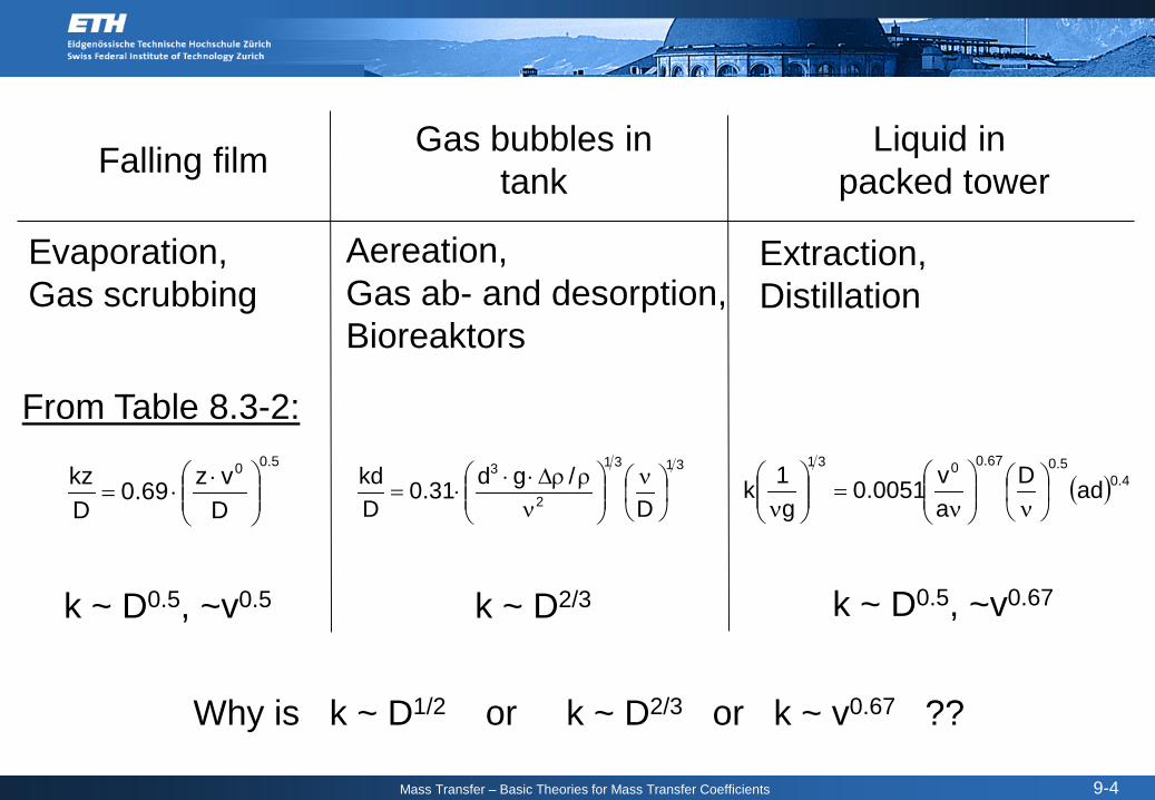
9.1 Fluid-Fluid Interfaces, e.g.

Falling film Gas bubbles intank

Liquid in packed tower

Source: Büchi Glas, UsterSource: Wikipedia, “Blasensäule”Source: Cussler, Chapter 2.5.2

Mass Transfer – Basic Theories for Mass Transfer Coefficients 9-4

Falling film Gas bubbles intank

Liquid in packed tower

5.00

Dvz69.0

Dkz

⋅⋅=

k ~ D0.5, ~v0.5

3131

2

3

D/gd31.0

Dkd

ν

ν

ρρ∆⋅⋅⋅=

k ~ D2/3

( ) 4.05.067.0031

adDav0051.0

g1k

ν

ν

=

ν

k ~ D0.5, ~v0.67

From Table 8.3-2:

Why is k ~ D1/2 or k ~ D2/3 or k ~ v0.67 ??

Aereation,Gas ab- and desorption,Bioreaktors

Extraction,Distillation

Evaporation,Gas scrubbing

Mass Transfer – Basic Theories for Mass Transfer Coefficients 9-5

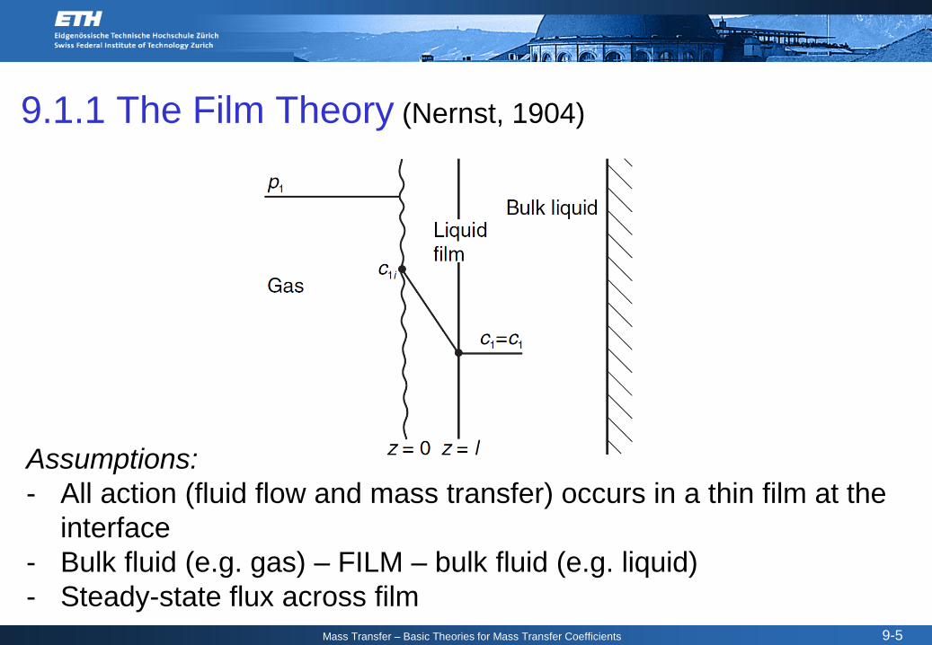
9.1.1 The Film Theory (Nernst, 1904)

Assumptions:- All action (fluid flow and mass transfer) occurs in a thin film at the

interface - Bulk fluid (e.g. gas) – FILM – bulk fluid (e.g. liquid)- Steady-state flux across film

9.1.1 The Film Theory (Nernst, 1904)

Mass Transfer – Basic Theories for Mass Transfer Coefficients 9-6

(9.1-1)

1 1 1i 1z 0

DN j (c c )=

= = −

(9.1-2)

Comparing equation (7.1) and (7.2) givesDk =

Or by rewriting gives k 1 ShD

= =

(9.1-3)

(9.1-4)

This simple theory gives k ∝ D1 BUT all fluid characteristics (e.g. fluid velocity due to stirring) are in the unknown film thickness .

This flux can be obtained also in terms of D (for dilute concentrations)

( )1i110z1 cckNn −===

Mass Transfer – Basic Theories for Mass Transfer Coefficients 9-7

This simple theory provides the FRAMEWORK of most MTC’s as follows:

mass transfer characteristic other coefficient lengthSh F system

diffusionvariables

coefficient

= =

Applications:

The film theory is used in some practical cases to determine the .

Mass Transfer – Basic Theories for Mass Transfer Coefficients 9-8

Example:CO2 is being scrubbed out of a gas by water flowing through a packed bed. Calculate the film thickness if 2.3·10-6 mol/(cm2∙s) of CO2 are adsorbed when

pCO2= 10 atm, H = 600 atm and DCO2/H2O= 1.9·10-5 cm2/s.

First find the interfacial concentration c1i :

1i1 1

cp H x Hc

= ⋅ =

1i3

-4 31i

c10atm 600atm (1 mol)/(18 cm )

c = 9.3 10 mol/cm

= ⇒

⋅

Solution:

Mass Transfer – Basic Theories for Mass Transfer Coefficients 9-9

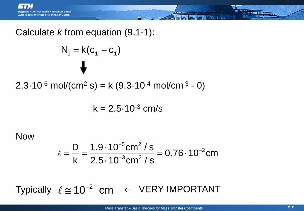
Calculate k from equation (9.1-1):

2.3·10-6 mol/(cm2 s) = k (9.3·10-4 mol/cm 3 - 0)

k = 2.5·10-3 cm/s

Now5 2

23 2

D 1.9 10 cm / s 0.76 10 cmk 2.5 10 cm / s

−−

−

⋅= = = ⋅

⋅

Typically cm 01 2−≅ ← VERY IMPORTANT

1 1i 1N k(c c )= −

Mass Transfer – Basic Theories for Mass Transfer Coefficients 9-10

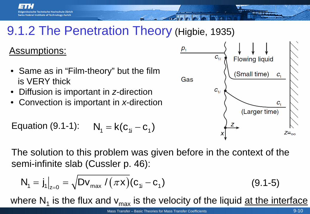
Assumptions:

• Same as in “Film-theory” but the filmis VERY thick

• Diffusion is important in z-direction• Convection is important in x-direction

1 1i 1N k(c c )= −Equation (9.1-1):

The solution to this problem was given before in the context of the semi-infinite slab (Cussler p. 46):

( )1 1 max 1i 1z 0N j Dv / x (c c )

== = −π (9.1-5)

where N1 is the flux and vmax is the velocity of the liquid at the interface

9.1.2 The Penetration Theory (Higbie, 1935)

Mass Transfer – Basic Theories for Mass Transfer Coefficients 9-11

Note that this flux at the interface is valid at a specific x. To find the average flux, N1(x) has to be averaged over the entire surface:

L W

1 1 z 00 0

1N n dy dxW L =

= ⋅⋅ ∫ ∫

cxvDL2N

L

0

max1 ∆

π⋅⋅

=

cLvDL2N max

1 ∆⋅π

⋅⋅=

where L is the length of the film in x and W is its width in y. Since n1does not vary in y, inserting 9.1-5:

∫ ∆⋅⋅π

⋅=

L

0

max1 dx c

xvD

L1N →

Mass Transfer – Basic Theories for Mass Transfer Coefficients 9-12

( )max1 1i 1

D vN 2 c cL

⋅= ⋅ −

⋅π

LvD2k max⋅π

⋅⋅= (9.1-6)so

The L/vmax is called contact time and is not known a priori in complex situations, as was in the film theory.

Compare:

(film theory)

1/2k D∝

k D∝

or

(penetration theory)

Mass Transfer – Basic Theories for Mass Transfer Coefficients 9-13

These two theories bracket the experimental data (Table 8.3-2) very well, almost too well to be accepted.Equation 9.1-6 can be rewritten, assuming that the average velocity is v0 = 2/3 vmax (true for a laminar slit flow of a Newtonian fluid).

12

12

1 2 1 2

Pe

6 Re Sc = π

21

02102

1

DLv6

LDv

23

DL2

DLk

π

=

π

=

=

212

102

1

DLv6

ν

ν

π

=

Mass Transfer – Basic Theories for Mass Transfer Coefficients 9-14

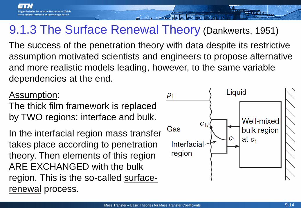
The success of the penetration theory with data despite its restrictive assumption motivated scientists and engineers to propose alternative and more realistic models leading, however, to the same variable dependencies at the end.

Assumption: The thick film framework is replaced by TWO regions: interface and bulk.

In the interfacial region mass transfer takes place according to penetration theory. Then elements of this region ARE EXCHANGED with the bulk region. This is the so-called surface-renewal process.

9.1.3 The Surface Renewal Theory (Dankwerts, 1951)

Mass Transfer – Basic Theories for Mass Transfer Coefficients 9-15

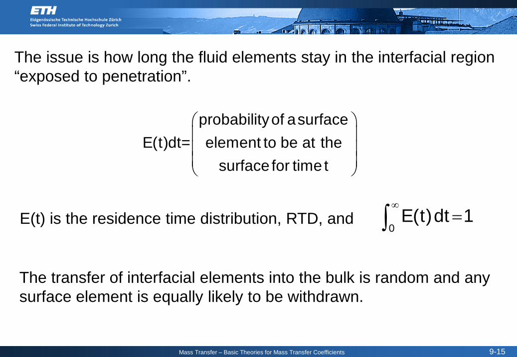
The issue is how long the fluid elements stay in the interfacial region “exposed to penetration”.

probabilityof asurfaceE(t)dt= element to be at the

surface for time t

E(t) is the residence time distribution, RTD, and0

E(t)dt 1∞

=∫

The transfer of interfacial elements into the bulk is random and any surface element is equally likely to be withdrawn.

Mass Transfer – Basic Theories for Mass Transfer Coefficients 9-16

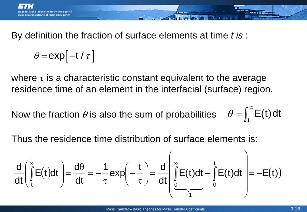
By definition the fraction of surface elements at time t is :

[ ]exp t /= −θ τ

where τ is a characteristic constant equivalent to the average residence time of an element in the interfacial (surface) region.

Now the fraction θ is also the sum of probabilitiest

E(t)dt∞

= ∫θ

Thus the residence time distribution of surface elements is:

( ) ( ))tEdt)t(Edt)t(Edtdtexp1

dtddttE

dtd t

0

1

0t

−=

−=

τ−

τ−=

θ=

∫∫∫

=

∞∞

Mass Transfer – Basic Theories for Mass Transfer Coefficients 9-17

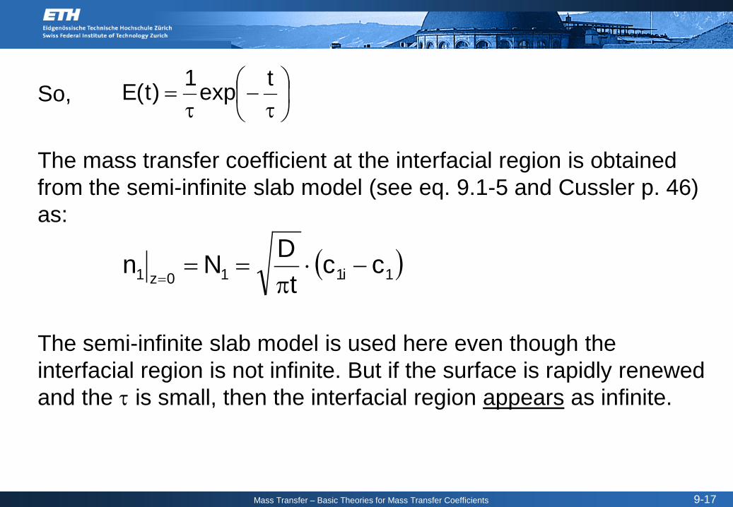
The mass transfer coefficient at the interfacial region is obtained from the semi-infinite slab model (see eq. 9.1-5 and Cussler p. 46) as:

The semi-infinite slab model is used here even though the interfacial region is not infinite. But if the surface is rapidly renewed and the τ is small, then the interfacial region appears as infinite.

So,

τ−

τ=

texp1)t(E

( )1i110z1 cct

DNn −⋅π

===

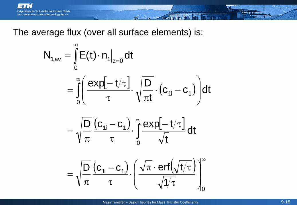
Mass Transfer – Basic Theories for Mass Transfer Coefficients 9-18

The average flux (over all surface elements) is:

∫∞

=⋅=

00z1av,1 dtn)t(EN

[ ] ( ) dt cct

Dtexp

01i1∫

∞

−⋅

π⋅

ττ−

=

( ) [ ] dt ttexpccD

0

1i1 ∫∞ τ−⋅

τ−

π=

( ) ( ) ∞

τ

τ⋅π⋅

τ−

π=

0

1i1

1terfccD

Mass Transfer – Basic Theories for Mass Transfer Coefficients 9-19

As in the penetration theory, here 1/2k D∝

Again the residence time τ is as unknown as the in film theory or the L/vmax (contact time) in the penetration theory.

The major contribution of the surface renewal theory is that it gives a more REALISTIC physical situation. This gives a better starting point for development of effective correlations and better models.

k D /= τ

( )1i1av,1 ccDN −τ

=

( ) ( ) ( )

τ−τ∞⋅πτ⋅

τ−

π=

==

01

1i1av,1 0erferfccDN

Thus,

Mass Transfer – Basic Theories for Mass Transfer Coefficients 9-20

Summary:

The Film Theory

The Penetration Theory

The Surface-Renewal Theory

LvD2k max⋅π

⋅⋅=

k D /= τ

k 1D

=

Advantages Disadvantages

Simple;good base for extension

Film thickness is unknown

Simplest including flow

Contact time (L/vmax) usually unkown

Similar math to penetration theory, but better physical picture

Surface-renewal rate (τ) is unknown

Mass Transfer – Basic Theories for Mass Transfer Coefficients 9-21

These simple models for fluid-fluid interfaces pretend that fluid motion is incorporated in diffusion and everything is treated as a thin film or semi-infinite slab problem.

In principle, these two extreme cases should bracket all possible geometries. Yet, especially the effect of flow (velocity) is usually not well reflected.

One reason is that the simple theories assume a homogeneous system while real systems are heterogeneous with respect to concentration and flow (Schlünder, 1977).

The dependencies of k on D and v, like k ~ D1/2, k ~ D2/3 or k ~ v0.67,observed in the experimentally-based MTCs are typically not well reflected by the simple mass transfer models.

Schlünder E.U., Chem. Eng. Sci. 32, 845-851.