Master thesis for the Master of Economics degree

Monetary policy and asset prices Interest rate rules and asset prices in Norway

Dag Klaveness

February, 2006

Department of Economics

University of Oslo

i

Preface I would like to thank my supervisor Hilde C. Bjørnland for her guidance and support. This

thesis was partially inspired by her lectures on Monetary Policy and Business Fluctuations

during the spring of 2005 and partially on her paper "Identifying the interdependence

between US monetary policy and the stock market" written with Kai Leitemo (2005).

The empirical work in this thesis has been performed using GiveWin 2.02 / PcGive.

ii

Contents 1. Introduction .................................................................................................................... 1

2. Monetary policy and simple interest rate rules ........................................................... 4

2.1 Monetary policy in a New Keynesian framework.................................................... 5 2.2 Targeting rules.......................................................................................................... 6 2.3 Instrument rules........................................................................................................ 8

3. Monetary policy and asset prices ................................................................................ 12

3.1 Asset price determination and interest rates........................................................... 13 3.2 The effect of asset prices on monetary policy........................................................ 14 3.3 Asset prices as an explicit target?........................................................................... 15 3.4 Asset prices and simple interest rate rules.............................................................. 18 3.5 Empirical issues related to interest rate rules and asset prices ............................... 19

4. Price misalignments in asset markets......................................................................... 22

4.1 Frictions in asset markets and asset price bubbles ................................................. 22 4.2 Price misalignments in the Norwegian stock market ............................................. 26

5. Empirical results........................................................................................................... 38

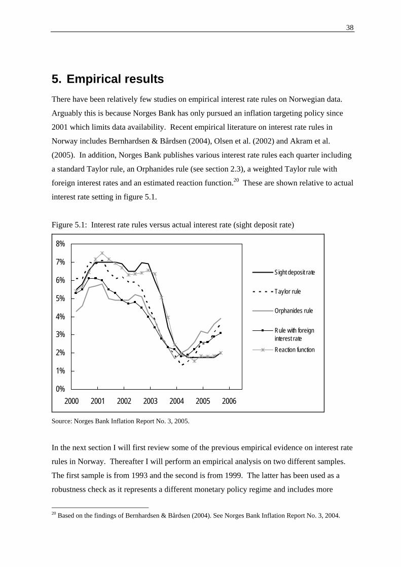
5.1 Previous empirical evidence................................................................................... 39 5.2 Data and methodology............................................................................................ 41 5.3 Interest rate rules in Norway from 1993 ................................................................ 42 5.4 Asset prices in a simultaneous model from 1993................................................... 43 5.5 Robustness check with data from 1999.................................................................. 45

6. Conclusion..................................................................................................................... 48

Appendix 1: Data description and unit root tests............................................................. 54

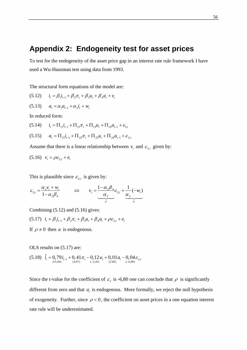
Appendix 2: Endogeneity test for asset prices .................................................................. 56

1

1. Introduction The purpose of this thesis is to survey and investigate the role of asset prices, in particular

stock prices, on monetary policy in Norway.1 There has been a long established consensus

in the literature that asset prices should not be targeted explicitly and that asset prices have a

limited role on monetary policy. However, recent contributions in the literature have argued

that asset prices might have a more prominent role due to their forward looking nature. This

thesis will survey some of these contributions and perform an empirical investigation on

interest rate rules and asset prices on Norwegian data.

Modern monetary policy, which incorporates inflation targeting, is founded on the New

Keynesian literature. The New Keynesian literature assigns a role to monetary policy in the

short-run due to the presence of nominal price rigidities and assumes optimizing households

and firms. However, it does not fully incorporate the adverse effects of severe asset price

misalignments for at least two reasons. First, household optimization implies intertemporal

consumption smoothing which in turn assumes somewhat stable asset prices since they

provide for a predictable store of wealth. The existence of severe asset price misalignments,

which are prevalent in most asset markets, implies that households may act sub-optimally

since such misalignments may significantly impact their lifetime savings. Second, the

literature has generally downplayed the role of investments since adding a variable capital

stock does not significantly change the overall results (see e.g. McCallum & Nelson (1999)).

However, recent studies have found that variability in capital utilization may be an important

prerequisite for inflation persistence (see e.g. Dotsey & King (2001) and Christiano et al.

(2001)), which may suggest that asset price volatility is desirable.

There is a consensus in the literature that asset prices should not be targeted explicitly.

Aside from the argument concerning capital utilization, this is due to the uncertainty

surrounding the identification of asset price misalignments and the uncertain effects

interventions may have on asset markets. This is not to say that there is no role for asset

prices in New Keynesian models. Some of the literature has argued that asset prices may

1 In the context of this thesis asset prices shall refer to stock prices only. Other forms of assets that serve as stores of wealth such as real estate, physical capital etc. have been ignored for simplicity although the fundamental analysis is the same. While foreign exchange deposits might be thought of as asset prices they are treated differently in the literature and this thesis will adhere to this differentiation.

2

contain information regarding future inflation not found elsewhere, mainly due to the their

forward looking nature (see e.g. Cecchetti et al. (2000)). Other reasons for why asset prices

may have an important role are the existence of market frictions such as agency problems

and market incompleteness. Much of the literature ascribe such frictions as the cause of

severe asset price misalignments (e.g. asset price bubbles). Although the adverse effects

asset price bubbles may have on the real economy have been thoroughly discussed in the

literature, they have been discussed less so in the context of monetary policy.

There exist several empirical contributions on asset prices and monetary policy. Generally

the literature has focused on measuring the relative efficiency of interest rate rules with asset

prices using calibrated small structural (New Keynesian) models (see e.g. Bernanke &

Gertler (2001)). Empirically estimated interest rate rules (reaction functions) that

incorporate asset prices have received relatively little attention (one notable exception is

Chadha et al. (2003)). One reason for this is the existence a simultaneity problem between

asset prices and interest rates making the identification issue problematic. Another is the

measurement problem associated with identifying asset price misalignments.

However, asset prices could be included in empirically estimated interest rate rules provided

the simultaneity and measurement problems are appropriately addressed. To avoid the

simultaneity problem I have formulated a simultaneous interest rate rule model for Norway

where asset prices enter endogenously. In measuring asset price misalignments I have opted

to follow the methodology used by Borio & Lowe (2002) which is based on measuring the

asset price gap as the deviation in cumulative asset returns from trend. I find that this

methodology is consistent with other asset price determination methodologies.

Using Norwegian data from 1993, I find that asset prices enter significantly in a

simultaneous model estimated using two stage least squares (2SLS). I also find that asset

prices contain more precise information on future inflation than the output gap and the

growth gap, particularly in conjunction with the unemployment gap. This implies that asset

prices can be viewed as an alternative real-time variable to the output gap or alike. These

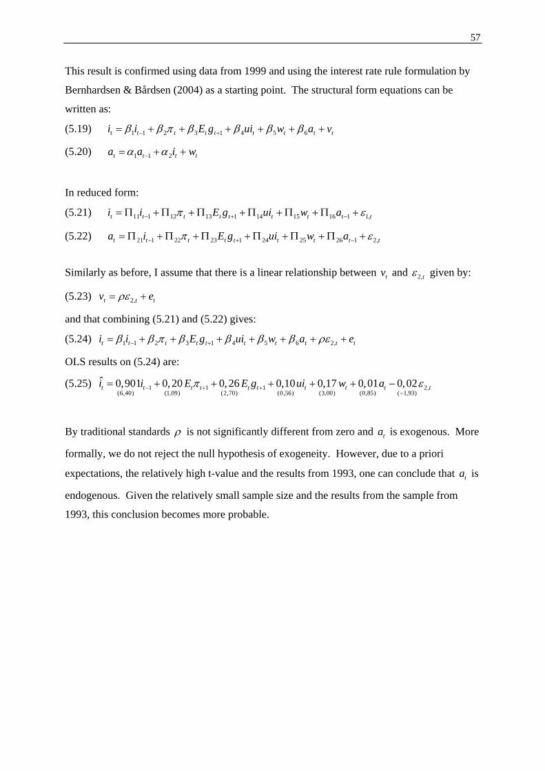
results are supported using more recent data from 1999. However, given limited data

availability more research is needed to ascertain the relative usefulness of asset prices on

monetary policy.

3

This paper is structured as follows. Section 2 gives an overview of monetary policy in a

New Keynesian framework and discusses some of the empirical challenges associated with

measuring interest rate rules. Section 3 surveys some of the literature on monetary policy

and asset prices and discusses some of the empirical challenges associated with measuring

interest rate rules with asset prices. Section 4 gives an overview of market frictions as the

causes of asset price misalignments, and discusses measurement and potential indicators.

Section 5 presents the empirical findings and Section 6 concludes.

4

2. Monetary policy and simple interest rate rules EQUATION CHAPTER 1 SECTION 2 It is widely accepted by most practitioners that modern monetary policy is best described in

a New Keynesian framework. New Keynesian models assign a role to monetary policy in

the short-run due to the presence of nominal price rigidities while building on the Real

Business Cycle literature and incorporating rational expectations. This is different from

traditional Keynesian models since aggregate demand only has short-term effects and long-

run output is determined by the production function (supply side) of the economy.

It is generally agreed in the literature that monetary policy in a New Keynesian framework

should aim to minimize the trade-off between inflation and output stability (see e.g. Clarida

et al. (1999)). Such a trade-off is minimized by so-called “flexible inflation targeting”. It is

also widely accepted that the interest rate is the preferred instrument choice of the central

bank although this is dependent on the types of shocks the economy is exposed to (see e.g.

Poole (1970)). The interest rate can either be set discretionary, according to a rule, or by a

combination of the two. A policy rule can in general help avoid the time-inconsistency

problem (inflation bias problem) and can therefore serve as a useful benchmark for

policymaking.

In the following sections I will discuss some of these results in more detail. First, I will give

an overview of monetary policy in a New Keynesian framework. Thereafter I will discuss

targeting rules and instrument rules respectively, and discuss how they are related. I will

also discuss why the central bank might want to use simple interest rate rules as a point of

reference in practical monetary policy and that an empirical interest rate rule may be thought

of as a central bank’s reaction function. Finally, I will discuss some of the empirical

limitations associated with such reaction functions.

5

2.1 Monetary policy in a New Keynesian framework The main implications for monetary policy in a New Keynesian setting are well summarized

in e.g. Clarida et al. (1999). They find that there is a role for monetary policy in the short-

run since prices are slow to react to fluctuations in aggregate demand and that there exists a

trade-off between high output and low inflation, and vice-versa. In the long-run, however,

monetary policy has no effect on output due to the assumption of a vertical Philips curve.

The New Keynesian framework has microeconomic foundations based on optimizing firms

and households. Firms are assumed to behave in a monopolistic competitive setting and

households are assumed to be utility maximizing. The optimization structure implies that

the framework in its basic form can be represented by two equations where monetary policy

can be viewed as affecting the real economy similarly to a traditional IS/LM model.

(2.1) 1 11 ( )t t t t t t ty E y i E uπσ+ += − − +

(2.2) 1t t t t tE ky eπ β π += + +

Equation (2.1) represents equilibrium aggregate demand. The difference between equation

(2.1) and a traditional IS curve is that it is derived from intertemporal household utility

maximisation (i.e. the Euler condition for optimal consumption). Hence, it is forward

looking in the sense that it incorporates both expected output gap ( ty ) and expected inflation

( tπ ). E is the expectations operator, σ is the intertemporal elasticity of substitution (which

comes from the utility function of the household), ti is the nominal interest rate, and tu is a

preferences (demand) shock. Equation (2.2) represents equilibrium aggregate supply

through what is often dubbed a “New Keynesian Philips curve”. It incorporates price

rigidities since changes in inflation are based on monopolistic competition where firms set

prices discretely (i.e. inflation persistence see e.g. Fuhrer & Moore (1995)). β and k are

constants and te is a cost shock.

It is worth noting, however, that the abovementioned equations are approximate solutions of

a more general equilibrium model. Further it is a simplified version of a more elaborate

model since it ignores investment, government spending, and foreign trade. Some studies

6

have found that the conclusions do not change significantly when altering the model to take

into account more variables (see e.g. McCallum & Nelson (1999) for investments).

The key distinction, however, between the New Keynesian framework and the traditional

IS/LM framework is the forward looking nature of the model. Credibility therefore plays an

important role. This is important since the interest rate is endogenous and the model needs

to be closed by an equation that describes monetary policy. That is, monetary policy needs

to be credible.

The traditional IS/LM model is closed with the LM curve. For this purpose, an LM curve is

superfluous since most of the literature generally agrees that the central bank’s reaction

function can be represented through a policy rule with the interest rate as the policy

instrument (see e.g. Bernanke & Mihov (1998)). This is founded on the time consistency

literature and the inflation bias problem (see e.g. Barro & Gordon (1983)). One of the

possible solutions to the inflation bias problem is the implementation of a policy rule that

dictates monetary policy over time. In general there are two types of rules: targeting rules

and instrument rules. It can be shown that adhering to a rule implies that optimal policy in a

theoretical framework is a linear relationship between the policy interest rate, inflation and

output (see eg. Walsh (2003) or Clarida et al. (1999)). However, it is possible that given a

more elaborate dynamical model that such a linear relationship may not necessarily hold.

There are therefore trade-offs between applying a targeting rule or an instrument rule and

these will be discussed in the following sections.

2.2 Targeting rules A targeting rule (such as an inflation target rule) aims at changing the policy interest rate so

that the target variable remains at its target level. The most common targeting rule is

inflation targeting. In its strictest sense, inflation targeting can be described as aiming

inflation around its target value at all times, or more formally at minimizing the following

loss function.2

(2.3) 2min ( *)t

t tLπ

π π= −

2 Illustrated as a quadratic function for simplicity

7

where π and *π are observed inflation and the inflation target respectively. However, in a

New Keynesian framework, as pointed out by Clarida et al. (1999), there exists a short-run

trade-off between inflation and output which implies that the loss function should be

formulated as:

(2.4) 2 2

,min ( *)

t tt t ty

L yπ

π π λ= − +

where y and λ is the output gap and the weight put on the output gap respectively (note

that 0 1λ< < ). This is commonly referred to as flexible inflation targeting. However, due

to interest rate smoothing the loss function is likely to be dynamic, as pointed out by Clarida

et al. (1999). That is, the central bank not only minimizes the loss function in the current

period, but in all future periods as well. Hence the loss function can be formulated as:

(2.5) 2 2

0( *)i

t t t ti

L E yβ π π λ∞

=

⎡ ⎤= − +⎣ ⎦∑

where β is the discount factor. Much of the literature uses such a dynamic loss function as

a discretionary assumption.3

A targeting rule has some important advantages. First, it is optimal since it follows

household optimisation and profit maximisation from the New Keynesian framework.

Second, it takes into account all relevant variables in the model and represents therefore the

optimal solution. Third, it is a fairly realistic assumption that central bank’s aim to optimize

their decision making. Unfortunately there are some major drawbacks. First, it is

complicated to solve and requires the central bank to make several assumptions regarding

some of the key variables, specifically β and λ . Hence, misspecification is likely. Second,

it is model dependent and therefore relatively less robust than an instrument rule. Third, it

will likely yield a too aggressive monetary policy unless lagged variables are included. This

implies that deviations are costly which in turn reduces the optimality of the rule unless such

costs are incorporated into the model. Fourth, and perhaps most importantly, it is not time-

3 This is based on the finding that equation (2.5) is a linear approximation of the optimal objective function in a New Keynesian setting (see e.g. Woodford (2001)).

8

consistent since the loss function is re-optimised in each time period which may give rise to

an inflation bias.

2.3 Instrument rules An alternative to deriving an optimal objective function is an instrument rule. Instrument

rules incorporate simple interest rate rules (among others) where the interest rate is set

according to a policy rule. As shown in Clarida et al. (1999) and Walsh (2003), adhering to

a monetary policy rule implies that optimal policy in a theoretical framework is a linear

relationship between the policy interest rate, inflation and output. Such a linear relationship

can be shown as:

(2.6) 0 1 2( *)t t ti yβ β π π β= + − +

where i , *π π− , and y are the policy interest rate, the inflation gap and the output gap

respectively. Note that the coefficient 0β indicates the steady state real interest rate plus the

inflation target. Also, it is generally required that the nominal interest rate has to change

more than the change in inflation in order to affect real interest rates (see eg. Clarida et al.

(1999)). A linear relationship such as in (2.6) was initially found by Taylor (1993), hence

the term “Taylor rule”. The Taylor rule simply expresses the FED’s reaction function in the

form of a simple interest rate rule using data from 1984 to 1992:4

(2.7) 4 1,5( *) 0,5t t ti yπ π= + − +

Although it must be emphasised that Taylor chose his coefficients using informal judgement,

his findings seem to track the actual policy interest rate in the period remarkably well,

despite the Federal Reserve not having adopted an inflation target. Similar results have been

found for Norway albeit not without some empirical difficulties. These will be discussed in

more detail in the next section.

Clarida et al. (1999) argue that the Taylor rule should be modified for two reasons. First,

they argue that a simple interest rate rule should be forward looking. This is consistent with

the optimal policy rule derived from combining the New Keynesian IS curve and the forward 4 Assuming an inflation target of 2%

9

looking Philips curve (as shown in equations (2.1) and (2.2)) and a simple linear response

rule between inflation and output (see Walsh (2003) or Clarida et al. (1999) for a formal

derivation). In addition, they argue that the rule is likely to be dynamic to incorporate that

central banks tend to change interest rates gradually. So-called interest rate “smoothing” has

been embraced in the theoretical literature by e.g. Brainard (1969) and Walsh (2003).

Brainard (1969) argues that parameter uncertainty implies that policy makers should behave

cautiously and Walsh (2003) argues that interest rate smoothing may arise from a desire to

ensure financial stability.5

In light of this, Clarida et al. (1999) formulate an interest rate rule with expected inflation

instead of current inflation and with a lagged interest rate variable to incorporate interest rate

smoothing.

(2.8) [ ]ttttt yEii 21101 *)()1( βππββρρ +−+−+= +−

They argue that the Taylor rule is a special case of a more general rule as formulated above,

when expected inflation is unavailable and interest rate smoothing is ignored. A formulation

with a lagged interest rate is also the starting point of most empirical work on interest rate

rules, although there is considerable disagreement on the relative size its coefficient (i.e. ρ ).

There are several advantages of applying simple interest rate rules to monetary policy. They

are simple, intuitive and time consistent. They also seem to track actual monetary policy

reasonably well and are in general more robust than targeting rules since they are not model

dependent and may be applied under a variety of assumptions and monetary policy regimes.

However, their simplicity is also their main drawback. Simple interest rate rules may not

always be optimal since they do not aim at completely neutralizing demand shocks as under

a targeting rule.6

Interest rate rules may also be inflexible to special situations. There may under certain

conditions be variables relevant to policy making other than inflation and output. One

5 However, Rudebusch (2002) argues that interest smoothing behaviour may imply that the policy maker will act sub-optimally. Further, Lansing (2002) attributes interest smoothing as an illusion caused by real time information problems. An alternative interpretation for interest rate smoothing is that interest rates have inertia. 6 This is because equation (2.1) now becomes relevant for determining interest rates. See Walsh (2003) p. 549 for a formal derivation.

10

example of this is the exchange rate, particularly for small open economies. Another

example is asset prices which in extreme circumstances may adversely affect the real

economy. Both of these will be discussed further in section 3.5

Given their drawbacks, it follows that simple interest rate rules should be used with a high

degree of caution and at most as reality checks in conjunction with a targeting regime.

McCallum (1999) argues that a good interest rate rule is one that is robust to different

modelling assumptions. Much of the econometric literature has therefore aimed at finding

simple relationships that can be used in a wide spectre of situations.

2.3.1 Empirical Issues:

Unfortunately, econometric work has shown that a simple interest rate rule such as that

proposed by Taylor (1993) fail to describe real time monetary policy with a reasonable

degree of efficiency. There are at least two reasons for this. First, there is uncertainty

related to measuring the steady state level of the output gap, and second, some of the

variables are subject to significant revisions over time.

Steady state/trend:

Estimating steady state or trend output is associated with a high degree of uncertainty since

most macroeconomic variables are non-stationary. Bjørnland et al. (2004) gives a good

overview of how to extract non-stationary trends. In general there are two methodologies.

One way is using a statistical detrending method such as a Hodrick-Prescott (HP) filter,

which is the preferred methodology of Norges Bank.7 An HP filter allows for a discretionary

weight (λ ) between a stochastic and a deterministic trend and is given by the following:

( ) ( ) ( )*

1 22* * * * *1 1

1 1

mint

T T

t t t t t ty t t

y y y y y yλ−

+ −= =

⎧ ⎫⎡ ⎤− + − − −⎨ ⎬⎣ ⎦⎩ ⎭∑ ∑

where *y is potential output. A 0λ = implies a stochastic trend and a λ →∞ implies a

deterministic (linear) trend. The main advantage of an HP filter is that it is very simple to

7 See e.g. Norges Bank’s Inflation Report No. 1 (2003).

11

use. The drawbacks are that they choice of λ is subject to discretion and that the end points

of the time series are likely to yield a too stochastic trend.

Another method is to use a multivariate methodology such as a production function or a

structural vector autoregression (SVAR). Regardless of methodology, the results are likely

to be imperfect due to the stochastic properties of the data which gives rise to uncertainty.

Although in general all models yield similar results, they may diverge significantly over

shorter time periods which is a serious drawback (see Bjørnland et al. (2004) for more

details).

Data revision:

Some economic time series are subject to considerable revisions over time relative to the

initially published figures. In particular this is related to output data such as GPD and

productivity. One possible solution to this problem has been proposed by Orphanides et al.

(2000). They find that the growth gap (actual growth less steady state growth) is subject to

less revision than the output gap and formulate an interest rate rule where the output gap is

replaced by the growth gap. Although their results are specific for the U.S. there are reasons

to expect that data revisions are of the same concern in all countries including Norway, (see

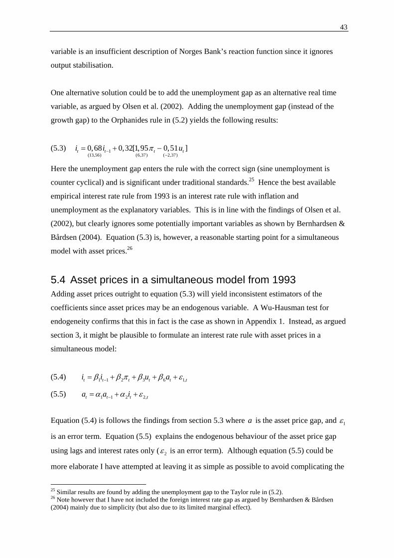
Bernhardsen et al. (2004)).

On Norwegian data, Olsen et al. (2002) finds that for the period 1995-1999 mainland GPD

growth was revised up by on average 1% per year, which suggests that there is considerable

uncertainty related to the growth gap as well. They further argue that other variables such as

the unemployment gap or the combination of the credit gap and the wage gap, can achieve

better results. Bernhardsen & Bårdsen (2004), however, shows that the unemployment gap

is not significant and argues that the estimated growth gap for the next 12 months is the most

appropriate measure. However, one thing these studies have in common is the relatively low

size of the coefficient of the output parameter and in some cases the relative low significance

levels. Hence, despite the vast amount of empirical literature available, the real time

problem for empirical interest rate rules remains unsolved.

12

3. Monetary policy and asset prices EQUATION CHAPTER 1 SECTION 3 The traditional view on asset prices and monetary policy in New Keynesian framework is

that they play no role. This is founded on the New Keynesian literature which assumes

optimizing households and firms. However, New Keynesian models do not fully incorporate

the adverse effects of severe asset price misalignments for at least two reasons. First,

household optimization implies intertemporal consumption smoothing which in turn assumes

somewhat stable asset prices since they provide for a predictable store of wealth. The

existence of severe asset price misalignments, which are prevalent in most asset markets,

implies that households may act sub-optimally since such misalignments may significantly

impact their lifetime savings. Second, the literature has generally downplayed the role of

investments since adding a variable capital stock does not significantly change the overall

results (see e.g. McCallum & Nelson (1999)). However, recent studies have found that

variability in capital utilization may be an important prerequisite for inflation persistence

(see e.g. Dotsey & King (2001) and Christiano et al. (2001)), which may suggest that asset

price volatility is desirable. This view regarding the capital stock is supported by other New

Keynesian type models such as RBC models with balance sheet effects (see e.g. Arnold

(2002)).

Severe asset price misalignments are prevalent in most asset markets and much of the

literature ascribes the causes of asset price misalignments to exogenous factors such as

agency problems and/or behavioral reasons. Asset price bubbles are examples of this. The

adverse effects asset price bubbles may have on the real economy have also been thoroughly

discussed in the literature, albeit less so in the context of monetary policy. Frictions in

financial markets are therefore likely to give asset prices a more prominent role in monetary

policy than what the traditional view advocates. Booms and busts in asset prices are

undoubtedly bad for the real economy and history is plentiful of examples. Borio et al.

(1994) shows that volatile asset prices (asset bubbles) have been an important factor in

explaining business cycles in both industrial and developing countries. Gerdurp (2003)

show similar results for Norway.

13

In the following section I will discuss the inclusion of asset prices in monetary policy rules.

First, I will give a brief overview of what determines asset prices how asset prices are

affected by monetary policy. Second, I will discuss the impact asset prices may have on

monetary policy. Third, I will discuss explicit targeting versus using asset prices as an

information variable. In so doing I will discuss asset prices in a theoretical framework where

I survey and discuss some of the main findings in the literature. Last, I will discuss asset

prices in a practical framework in terms of interest rate rules where among other things I will

discuss the simultaneity issue between asset prices and monetary policy.

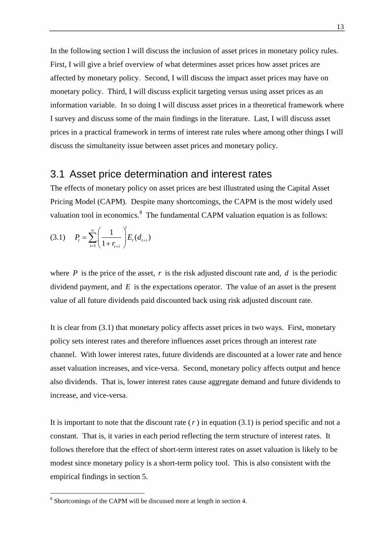
3.1 Asset price determination and interest rates The effects of monetary policy on asset prices are best illustrated using the Capital Asset

Pricing Model (CAPM). Despite many shortcomings, the CAPM is the most widely used

valuation tool in economics.8 The fundamental CAPM valuation equation is as follows:

(3.1) 1

1 ( )1

i

t t t ii t i

P E dr

∞

+= +

⎛ ⎞= ⎜ ⎟+⎝ ⎠∑

where P is the price of the asset, r is the risk adjusted discount rate and, d is the periodic

dividend payment, and E is the expectations operator. The value of an asset is the present

value of all future dividends paid discounted back using risk adjusted discount rate.

It is clear from (3.1) that monetary policy affects asset prices in two ways. First, monetary

policy sets interest rates and therefore influences asset prices through an interest rate

channel. With lower interest rates, future dividends are discounted at a lower rate and hence

asset valuation increases, and vice-versa. Second, monetary policy affects output and hence

also dividends. That is, lower interest rates cause aggregate demand and future dividends to

increase, and vice-versa.

It is important to note that the discount rate ( r ) in equation (3.1) is period specific and not a

constant. That is, it varies in each period reflecting the term structure of interest rates. It

follows therefore that the effect of short-term interest rates on asset valuation is likely to be

modest since monetary policy is a short-term policy tool. This is also consistent with the

empirical findings in section 5.

8 Shortcomings of the CAPM will be discussed more at length in section 4.

14

The long-term effect of monetary policy on asset prices can be easily illustrated if we re-

write (3.1) assuming dividends grow at a constant (steady state) rate:9

(3.2) 1( )ˆt t

tE dP

r g+=

−

where g is the dividend growth rate and r is the long-run expected return on the asset. This

formulation however requires that both r and g are constant and that r g> . Equation (3.2)

implies that short-term interest rates, and hence monetary policy, have no effect on asset

valuation in the steady state. Correspondingly, if monetary policy is not aimed at affect

long-term economic performance it should not affect long-term interest rates nor steady state

asset valuation.

3.2 The effect of asset prices on monetary policy In text-book macroeconomic theory (i.e. in an AD-AS framework), asset prices affect

aggregate demand through consumption and investments. That is, higher asset prices lead to

increased consumption and increased investments. In a traditional aggregate demand

equation this can be formulated as:

(3.3) ( , , ,...) ( , ,...) ...Y C w mf I q c+ + + + +

= Ω + +

where Ω is household wealth, w is household wages, mf is the level of market frictions, q

is the ratio indicating the replacement cost of capital (Tobin’s q), and c is the amount of

collateral available (+/- signs indicate the sign of the partial derivative w.r.t. their respective

functions).

Consumption is affected by asset prices through three channels. First, lifetime wealth is

affected by asset prices and inevitably so is consumption since wealth is the premises for

consumption smoothing. Second, higher asset prices affect household expectations of future

wages since firms are expected to earn higher profits, and vice-versa. Third, consumption

smoothing is distorted by imperfect capital markets which makes agents more sensitive to 9 Sometimes referred to as the Gordon growth model, see Gordon (1962).

15

current events (as opposed to future events). The two former channels are incorporated into

the New Keynesian framework through the assumption of household intertemporal utility

maximisation. The latter channel is somewhat overlooked and implies that asset price

volatility distorts household’s optimising behaviour.

A key question in this connection is the elasticity of consumption with respect to asset

prices. Obviously this elasticity needs to be sufficiently high for asset prices to have an

effect. There have been some findings that support this, particularly for stock markets in the

US, but the empirical evidence suggest that this relationship is weak in European countries

(see e.g. IMF (2000)). One explanation for this may be the smaller share of stock ownership

relative to financial assets in European countries and that real property prices may play a

larger role.

Investments are affected by asset prices through two channels. First, changes in asset prices

affect the decision to invest relative to the replacement cost of capital (Tobin’s q). That is,

higher asset prices means that the replacement cost is low hence firms will invest more

(since there are arbitrage opportunities in the secondary market). Second, changes in asset

prices affect the ability of firms to provide collateral and hence affect their cost of capital

(credit channel). Similarly to the wealth effect, empirical evidence suggests that investments

are more sensitive to asset prices in the US relative to Europe (see e.g. IMF (2000)).

Unfortunately, no study to date has investigated the combined elasticity of the stock market

and house prices on both consumption and investment and hence the relative role of asset

prices in the US and Europe remains inconclusive.

3.3 Asset prices as an explicit target? Much of the debate in the economic literature concerning asset prices is whether asset prices

should be targeted explicitly or if they are only useful as an information variable for future

inflation (see e.g. Chadha et al. (2003) and Bjørnland & Leitemo (2005)). Arguments in

favour of targeting asset prices explicitly are primarily based on the idea that frictions in

financial markets may lead to unsustainably high asset prices (e.g. asset price bubbles)

which, if not addressed, may have adverse effects on the real economy (such frictions are

discussed at more length in section 4). Aside from the argument concerning capital

utilization, arguments against are based on the uncertainty surrounding the identification of

asset price misalignments and the uncertain effects potential remedies may have on asset

16

markets. The consensus in the literature therefore seems to favor that asset prices should not

be targeted explicitly. However, asset prices may still be a useful variable due to its forward

looking nature as discussed in section 3.1. That is, asset prices may contain information

regarding future inflation not found elsewhere.

The traditional theoretical view on asset prices and monetary policy is that asset prices play

no role in an inflation targeting regime. Proponents of this view are Bernanke & Gertler

(1999) and Bean (2003), among others. Bernanke & Gertler (1999) constitute the main

theoretical argument for not including asset prices in monetary policy decision making.

They argue that the central bank does not have sufficient information to correct for price

misalignments in asset markets. Using a theoretical model with sticky prices, they show that

as long as the central bank reacts aggressively to inflation, it also prevents asset price

misalignments from occurring. Bean (2003) reviews the role of asset prices and similarly

concludes that optimal policy is sufficiently embraced by flexible inflation targeting.

Some objections need to be made. First, central banks rarely react aggressively to inflation.

This is advocated by so-called “flexible inflation targeting” which implies that central bank

adjusts their policy interest rate gradually (or more formally have a flexible time horizon).

Second, it is not obvious that central banks do not have sufficient information to react to

asset price misalignments. Cecchetti et al. (2000) argue that identifying asset price

misalignments is not fundamentally different from identifying the output gap or the

equilibrium real interest rate. In that respect, since the central bank must make an

assessment of the output gap by making a qualified “guess” of what constitutes potential

output, there is no reason why they could not do the same with asset prices.

There is an abundance of theory based literature that advocates the use of asset prices in

monetary policy, all of which focus on the presence of frictions in asset markets. Most

notable are the works by Borio & Lowe (2002), Carlstrom & Fuerst (2001) and Cecchetti et

al. (2000). Borio & Lowe (2002) argue that financial distress can build up in an inflation

targeting regime for two reasons. First, an adverse selection problem may arise since stable

interest rates will likely lead to easier access to credit and hence poor lending decisions are

more likely. Second, if the central bank is credible, prices will be more sticky and hence

investors will take higher risks. They suggest that the central bank should react to such

imbalances when appropriate.

17

Calstrom & Fuerst (2001) develops a theoretical model similar to that of Bernanke & Gertler

(1999), but assumes that prices are perfectly flexible (which may not be realistic). They

show that there is a role for asset prices in monetary policy when there is imperfect

information and exogenous asset price shocks. Furthermore, their findings illustrate the

model dependency of the results since their results are the exact opposite of that of Bernanke

& Gertler (1999).

Cecchetti et al. (2000) also argue that optimal policy should take asset prices into account.

They argue that inflation forecasts depend on an assumption regarding asset prices hence

asset price misalignments may play a significant role. Although they develop no formal

model, they show econometrically that asset prices have a strong effect on future inflation.

They also argue that attempting to reduce asset price misalignments will reduce the

likelihood of asset price misalignments in the future. They do, however, acknowledge that

asset prices should not be targeted per se, only that asset prices should be used as an

indicator of future inflation.

From a practical view, the answer to whether asset prices should be targeted may be more

obvious. As argued by Bjørnland (2005a) fighting asset inflation or asset price

misalignments through explicit targeting may do more harm than good. That is, increasing

the policy interest rate due to asset price misalignments may have overly negative effects on

output through a stronger exchange rate and lower inflation. This is also supported by the

link between asset prices, investments and capacity utilisation may imply that volatile asset

prices are a prerequisite for inflation persistence (as argued by Dotsey & King (2001) and

Christiano et al. (2001)). It might therefore be that asset prices should not be targeted at all,

at least during normal circumstances when asset valuations are not unduly exuberant.

The view that asset prices can be viewed as an information variable is based on the forward

looking nature of asset prices since as discussed in section 3.1. Asset prices are forward

looking since they contain information about future dividend growth, future interest rate

levels and future risk premia. In the strictest sense, there is therefore no causal relationship

between asset prices and monetary policy (see e.g. IMF (2000)) provided the central bank is

at no informational disadvantage (see e.g. Bjørnland & Leitemo (2005)) and if there is no

18

policy regime change. That is, if the central bank has the same information set as that of the

asset market then information provided by the asset market is irrelevant.

One key assumption here is that the asset market is priced correctly based on aggregate

expectations and that fluctuations in asset markets reflect changing expectations and

fundamental reasons only. However, it t is not at all obvious that all fluctuations in asset

markets reflect changing expectations and fundamental reasons only, nor is it obvious that

markets are efficient, and there is an abundance of theoretical and empirical evidence to

support this (see e.g. Allen & Gale (1999, 2000a, 2000b) and Shiller (2003)). Frictions in

financial markets, particularly those related to agency theory, allow for price misalignments

in asset markets which may “cloud” the information extracted from asset markets, or at least

make it sufficiently different from the information set of the central bank. Asset prices may

therefore provide a good benchmark for economy wide expectations (which is what really

matters).

3.4 Asset prices and simple interest rate rules Although asset prices may have a role in monetary policy due to their informational content,

there is much disagreement in the literature whether they may have a role in simple interest

rate rules. Bernanke & Gertler (2001) rejects the use of simple interest rate rules with asset

prices altogether. They use simulation to compare various interest rates rules, with and

without asset prices, and measure how their models respond to various types of shocks.

They find that a policy rule that only takes into account inflation and output is the most

efficient. However, one problem with their methodology is that a simulation framework

does not aim to measure the central bank’s reaction function, but aims at measuring relative

efficiency. Another is that their model is highly simplified and does not take into account

other explanatory variables that may impact interest rates such as interest rate smoothing.

Simulation studies, or “new normative macroeconomic research” as dubbed by Taylor

(2001), are highly model dependent. This is well illustrated by the findings of Akram et al.

(2005) who finds that adding asset prices to an interest rate rule may improve

macroeconomic performance, which is the exact opposite of Bernanke & Gertler (2001).

They use Norwegian data from 1984-2000 and simulate macroeconomic performance when

adding asset price shocks. They find that variability in output and inflation decreases when

asset prices are included in the central bank’s reaction function.

19

Chadha et al. (2003) estimates empirical interest rate rules with asset prices using a GMM

methodology on data from the US, UK and Japan from 1979-2003. They argue that asset

prices should be used as an information variable concerning future inflation and that central

banks should use the policy interest rate to offset price misalignments in asset markets. They

find that asset prices are relevant when misalignments in asset markets are relatively large

implying that asset prices may enter into the central banks’ reaction functions. However,

they concede that asset prices may enter the reaction function non-linearly which suggests

that estimating interest rate rules with asset prices may be difficult.

Bordo & Jeanne (2002) argue along the same line, suggesting that adding asset prices to the

central bank’s reaction function may be optimal but that such a rule is unlikely to be linear.

They use two historical examples of when reacting to asset prices bubbles have gone afoul.

They argue that a contractionary monetary policy following the 1929 crash and Japanese real

estate bubble in the 1980s were sub-optimal since higher interest rates worsened the effects

on the real economy (see also Bordo et al. (2001)).

This illustrates well the dilemma when considering asset prices in monetary policy. If

interest rates are used as a tool to burst an asset bubble, the central bank may risk initiating a

financial crisis. Allen & Gale (1999, 2000a,b) argues that if a financial crisis occurs, the

central banks primary role should be to provide liquidity for ailing banks. This in turn

implies that interest rates should be lowered which may explain the non-linearity of the

central banks reaction function. However, so long as no financial crisis occurs, there are no

a priori reasons to expect that the central bank’s reaction function should be non-linear.

3.5 Empirical issues related to interest rate rules and asset prices

The interest rate and possible explanatory variables will in general be mutually dependent.

That is, one or more of the explanatory variables might be endogenous. Failing to account

for such endogeneity issues will yield inconsistent estimators. The inclusion of exchange

rates in interest rate rules for small open economies is a good example. The exchange rate

has a simultaneous relationship with interest rates. That is, higher interest rates generally

imply an appreciation of the exchange rate. A stronger currency generally implies higher

imports which in turn imply lower interest rates. It follows therefore that estimating an

20

interest rate rule with the exchange rate as an explanatory variable will yield inconsistent

estimates since the exchange rate is not exogenous. It may therefore be appropriate to

estimate the impact of the exchange rate using a simultaneous model where the exchange

rate is treated endogenously.

Much of the empirical work related to exchange rates is based on calibrated structural

macroeconomic models where various interest rate rules are tested based on different types

of shocks. Obstefeld & Rogoff (1995), Ball (1999) and Svensson (2000) all find that

simulated interest rate rules that include the exchange rate perform better than those without.

Taylor (2001) on the other hand argues that these improvements are relatively small and that

the exchange rate should not be targeted at all, even for small open economies. He argues

that there exists an indirect effect of the exchange rate on inflation and output, assuming a

rational expectations model of the term structure of interest rates and that the policy rule will

be used consistently over time. It has also been common to use simultaneous models to

account for the endogeneity of the exchange rate. One such example is Bernhardsen &

Bårdsen (2004) who estimates an interest rate rule with the exchange rate using Norwegian

data from 1999-2005 where they find that the effect of the exchange rate is significant.10

One objection to such a methodology is that it somewhat defeats the purpose of a “simple”

interest rate rule since the rule will be more model dependent and hence less robust.

Due to simultaneity, there are reasons to believe that asset prices may behave in a similar

fashion as the exchange rate. As discussed in section 3.1, asset prices are affected by

monetary policy since interest rates affect asset valuations through the discount rate.

Conversely, as discussed in section 3.2, asset prices affect monetary policy through variation

in aggregate demand which in turn affect interest rates.

This is supported by the empirical literature where the effect of monetary policy on asset

prices has been studied extensively. Traditional studies have largely found these effects to

be modest, although they point in the right direction. That is, higher interest rates lead to

lower asset prices (and vice-versa) and higher asset prices lead to higher interest rates (and

vice-versa). Event studies have tried to find the immediate effects between asset prices and

monetary policy; e.g. Bernanke & Kuttner (2004) finds that an unexpected rate increase of

10 Due to data limitations however, they estimate an interest rate rule with the foreign interest rate as an instrumental variable for the exchange rate under the assumption of interest parity.

21

25 basis points reduces asset values by 1 percent primarily due to lower equity risk

premiums. Rigobon & Sack (2004) have found similar results. However, event studies fail

to account for long-term simultaneity effects between asset prices and monetary policy

although Rigobon & Sack (2003) shows that increased asset prices increases the likelihood

of higher interest rates. Newer studies using structural vector autoregression (SVAR)

models find that the simultaneity effect is much stronger. Bjørnland & Leitemo (2005) find

a high degree of interdependence between asset prices and monetary policy. They show

with US data that a 10 basis point interest rate increase decreases asset valuations by 1,5%

and that an increase in asset valuations of 1% leads to 5 basis point interest rate increase.

Asset prices and monetary policy are therefore interdependent and should be modelled

simultaneously with both interest rates and asset prices as endogenous variables.

22

4. Price misalignments in asset markets EQUATION CHAPTER 1 SECTION 4 It is generally agreed that asset markets are not perfectly efficient (see e.g. Shiller (2003) and

Malkiel (2003) for an overview). Asset markets are subject to considerable noise which may

be persistent in the sense that valuation in asset markets can deviate from its fundamental

value over longer periods of time. Asset price bubbles are examples of this. There are at

least three factors that may cause asset markets to deviate from their fundamental value.

First, frictions in asset markets, particularly those related to principal-to-agent related issues,

signify that asset markets may be incorrectly priced. Second, there may be behavioural or

psychological effects that cause asset prices to have short-term momentum (see e.g. Shiller

(2003)). Third, asset prices may be subject to noise like any other economic variable simply

because there will be pricing disagreements among agents.

Frictions in financial markets have been widely studied, particularly those related to

principal-to-agent related issues. Such frictions may include liquidity rationing, risk

shifting, and convex incentive schemes of intermediaries, among others. These will be

discussed in more detail in the next section. Thereafter, in section 4.2, I will discuss some

methodologies for identifying price misalignments. I will also attempt to find a reliable

indicator for price misalignments in the Norwegian stock market that can be used for

empirical purposes.

4.1 Frictions in asset markets and asset price bubbles Traditionally, macroeconomic modelling has assumed complete markets, or markets without

the existence of frictions. The principle-agent literature, however, identifies several

“frictions” which may give rise to incomplete markets. The literature concerning asset price

bubbles and financial crises has ascribed the existence of incomplete markets as an important

contributing factor to the existence of asset price misalignments. Deviations in asset values

from their fundamental values can therefore be ascribed to market incompleteness.

Since information is costly, financial intermediaries have a prominent role in the functioning

of financial markets. That is, there is asymmetric information between principals and agents.

The presence of information asymmetries gives rise to the two most commonly noted market

23

frictions; the moral hazard problem and adverse selection problem. A moral hazard problem

arises when the interests of the principal and the agent are misaligned. An adverse selection

problem exists when there are information asymmetries between principals and agents and

the principal is forced make a sub optimal choice. Note that these frictions gives rise to even

more financial intermediaries since moral hazard and adverse selection gives rise to

monitoring (see e.g. Diamond (1991)), credit rationing (see e.g. Stiglitz & Weiss (1981)) and

increased quantity of money (see e.g. Bernanke & Blinder (1988)), among others.

Price misalignments due to frictions in asset markets are much discussed in the literature

concerning asset price bubbles and financial crises. Allen & Gale (2000a) define a positive

(negative) asset price bubble as an event where asset prices are above (or below) their

fundamental value.11 Little of the literature has focused on the sources of asset price bubbles

in isolation but has instead focused on explaining their occurrence jointly with financial

crises. Allen & Gale (1999) describe the development a typical financial crisis in three

phases:

1. Financial liberalisation or a conscious decision to increase lending bids up asset prices

due to agency problems and risk shifting.12 As asset prices increase, more collateral

becomes available to fund new loans and the bubble fuels itself.

2. The bubble bursts due to an exogenous real shock or exogenous financial shock.

3. A financial crisis develops since asset prices have collapsed and can no longer serve as

collateral for inflated credit levels.

Allen & Gale argue that financial liberalisation or a conscious decision to increase lending

bids up asset prices. In this respect they treat financial liberalisation as an exogenous event.

However, Shiller (2003) argues that much of the fluctuation in asset price markets may be

for behavioural (i.e. psychological) reasons. It is therefore plausible that if asset prices

increase sufficiently (for behavioural reasons) access to credit may in fact increase (since

bank officers may suffer from the same behavioural dysfunctions as the market) and the

bubble may initiate itself.

11 Although it may seem obvious that a small price misalignment is not necessarily a “bubble”, I will treat them as the same thing for the purposes of this discussion. 12 Risk-shifting occurs when providers of funds are unable to observe the risk level of the ultimate investments.

24

Asset prices are further inflated due to agency problems. These may include risk-shifting,

convex incentive schemes,13 increased liquidity and limited liability.14 However, the

existence of agency problems only means that there is an upward-bias in asset valuation. I

would argue that this is somewhat overlooked in the literature. It is not agency problems

that cause bubbles although their existence may have multiplicative effects. In that sense,

agency related problems and other market frictions might give higher persistence to noise in

asset markets.

Eventually the bubble will burst due to an exogenous real or financial shock. Allan & Gale

use the financial crisis in Norway (1988-92) and the oil shock in 1986 as an example of this.

However, Mankiw (1986) shows that in a theoretical framework financial collapse can occur

when asset price markets are in disequilibrium (i.e. in a bubble state) and that such a collapse

occurs due to adverse selection. Furthermore, I would argue that the behavioural reasons

mentioned earlier may serve in the opposite direction to end the bubble. Since future credit

growth is already “priced-in” in asset prices, any deviation from expectations may cause the

bubble to burst. Whether the burst is due to a real or financial exogenous shock, or due to

systemic imbalances is not that important. The main thing to notice is that the bubble will

burst sooner or later since credit is limited in supply.

Borio & Lowe (2002) argue that “other common signs [of asset price bubbles] include rapid

credit expansion and often, above-average capital accumulation” (p. 1). This is supported by

Allen & Gale (1999, 2000b) who develop a theoretical model which shows that the two most

important factors that influence the size of an asset price bubble is the amount of credit

available (and the expected amount of credit available in the future) and the degree of

uncertainty. That is, the higher the uncertainty and the higher the availability of credit, the

greater the potential price misalignment. Hence it is the combination of high credit growth

and asset prices in a bubble state that gives rise for concern since asset valuations serve as

collateral for bank credit.

It is also often argued that real estate prices play an important role in the formation of asset

price bubbles. Real estate assets are subject to the same bubble tendencies as equity markets

since they are both affected by the availability of credit. Further, real estate is arguably a

13 That is, financial intermediaries have unlimited upside in revenues but limited downside. 14 Investors can only lose as much as they have invested which gives rise to an asymmetric payoff profile.

25

more important source of household savings in some countries, particularly for Norway (see

e.g. IMF (2000)) and Hansen (2003) attributes real estate prices to be a predictor of

bankruptcies and therefore an indicator of macroeconomic imbalances. Following Borio &

Lowe (2002)’s argument, a rapid increase in credit, real estate prices, and or equity markets

in isolation pose little threat to financial stability, but jointly they increase the likelihood of a

financial crisis.

Borio & Lowe (2002) argues therefore that a combined index of credit growth, real estate

prices and equity markets could be a useful indicator for policy makers. Using cross country

annual data from 1960-1999 on a sample of OECD countries, they find that equity markets

and credit growth are in combination a reliable indicator of historical financial crises.

Although they recognize the importance of real estate prices, they are forced to ignore them

due to data limitations. Despite of this, their results are remarkably robust, hence I have

opted not to focus on real estate prices in analysis in the succeeding section, but noting that

real estate prices may in fact play an important role.

The main problem associated with asset price bubbles is the high probability of an ensuing

financial crisis. As Allan & Gale (1999) argue, “financial crises are often associated with a

significant fall in output or at least a reduction in the rate of output” (p.6). Why this is the

case is fairly obvious: if asset prices decline rapidly and asset prices serve as a source of

financial cash flow and as collateral for bank debt, borrowers will have a lower probability

of paying interest and repaying their loans. Hence there will be a higher default frequency.

This will in turn force banks to write-off bad loans and/or risk having a portfolio of bad

loans that is larger than their associated collateral. This may also force banks into

insolvency. Jointly this series of events may have adverse effects on the real economy for a

number of reasons. First, a banking crisis and/or a bank run may occur. Second, access to

credit will be severely constrained since banks will not be able to raise new capital which is

likely to lead to a lower investment rate. Third, households will be reluctant to save which

may affect their willingness to smooth consumption over time. Allen & Gale (1999) further

point out that for small economies this may put serious strain on the economy’s currency

since the central bank may be forced to lower interest rates to prevent banks from becoming

insolvent. This may have particular relevance for Norway. Additionally, there is strong

26

empirical evidence of a link between financial crisis and a drop in output (or a reduction in

growth), see e.g. Bernanke & Gertler (1989) and Gerdrup (2003) for Norway.15

It is clear therefore that asset price misalignments may undoubtedly be bad for the real

economy. The question then arises how policy makers should respond to such

misalignments. There are at least three approaches, depending on how far the bubble has

developed. First, policy makers can impose regulation and institutional structures such that

financial crises are unlikely to occur (see e.g. Bernanke & Gertler (1999)). Second, policy

makers can proactively try to prevent them by intervening when appropriate by e.g. raising

interest rates to reduce asset valuations and reduce the availability of credit. Third, policy

makers can reduce the impact of financial crises after they have occurred by e.g. lowering

the interest rate to provide more credit to ailing banks (see e.g. Allen & Gale (2000a)). Since

the appropriate response depends somewhat on how far the bubble has developed, it is likely

that the response function of policy makers with respect to asset prices is non-linear,

similarly to some of the findings in section 3.4.

4.2 Price misalignments in the Norwegian stock market There is much disagreement in the literature whether identifying asset price bubbles are at all

possible. Gurkaynak (2005) argues that there are several econometric problems with

identifying asset price bubbles using the CAPM. In light of this, many economists dismisses

the idea of asset prices in monetary policy outright (see e.g. Bernanke & Gertler (1999)).

However, as Cecchetti et al. (2000) points out, the difficulties associated with measuring

asset price misalignments are not substantially different from those associated with

measuring the output gap. I will therefore assume that asset price bubble identification is

possible.

To identify asset price misalignments one needs to make an assessment about what

constitutes fundamental value. There are at least three methodologies on how to evaluate the

fundamental value of aggregate asset markets. First there is the CAPM approach which has

already been discussed somewhat in section 3.1. Second, there is the Tobin’s q approach

which uses the ratio of observed asset values relative to their replacement cost. Third, there

15 In particular he finds reduced output following the financial crises of 1899-1905, 1920-28, and 1988-92.

27

is a much simpler but nonetheless effective approach of measuring the deviation in asset

returns from their long-run trend.

All three methodologies are based on the same economic principle: that there exists a steady

state valuation level since long-run corporate profits cannot grow faster than the economy as

a whole. In the short-run, however, there might be more variables affecting asset valuations

such as risk shifting or behavioural reasons as pointed out in the previous section. Such

frictions imply that evaluating short-run asset valuations is not an exact science and there

might be considerable room for disagreement, which of course is the reason why asset

markets are so volatile. Other variables affecting short-term valuations, such as access to

natural resources, will for the purposes of this paper be ignored since they are unlikely to

affect short-term policy decisions.

4.2.1 The CAPM approach:

The CAPM says that the periodic return on any asset is the periodic risk free rate plus a risk

premium that reflects the risk level of the asset:

(4.1) , , ,( ) ( )t i t f t i m f tE r r r rβ= + −

where ,i tr is the return on asset i in period t , ,f tr is the risk free return in period t , mr is the

return on the market portfolio, iβ is the risk coefficient of asset i relative to the market and

E is the expectations operator. However, it is worth noting that the formulations in (4.1) is

related to individual assets. When valuing the aggregate asset market (4.1) can be written as:

(4.2) ,( )t i t mE r r=

since the β of the aggregate asset market must be 1. This is important since it implies in the

long run asset valuations are determined by economy wide characteristics only. It is

plausible, however, that the expected return may fluctuate in somewhat in the long-run

reflecting e.g. the level of competition (see e.g. Smithers & Wright (2000)).

The CAPM has many shortcomings. The most important is probably that pointed out by

Shiller (2003) which is that the CAPM cannot explain much of the volatility in asset

28

markets. Most economists therefore agree that the CAPM only serves as a long-term

valuation guideline and that short-term asset prices are subject to considerable noise. It may

appear therefore that the traditional CAPM methodology may be incorrectly specified, that it

fails to account for important variables, or at least that it only serves as a representation for a

steady state solution.

There has been much debate in the literature on the validity of the CAPM, most of which has

been centred on whether the CAPM is at all testable. The untestability of the CAPM is well

summarized in Roll (1977). Roll ascribes the untestability of the CAPM to the identification

problem of the true market portfolio and that the only valid conclusion one can draw from

testing the CAPM is that there is insufficient data available. Other problems with the CAPM

are mostly related to its assumptions and how the model is applied. The CAPM is founded

on some fairly unrealistic assumptions which are sometimes overlooked. First, the CAPM

defines risk as the covariance of future returns with other asset markets in general. This is a

fairly narrow definition which ignores risks such as default risk and the fact that risk is

heavily right-skewed due to market frictions. Second, for practical purposes there is no such

thing as a truly risk-free interest rate since there is no guarantee that central banks cannot go

bankrupt. Third, there is ample empirical evidence that asset markets are not perfectly

efficient (see e.g. Shiller (2003) for an overview).

Despite its weaknesses the CAPM is widely used in financial markets and is the most

frequently used model to identify asset price misalignments. Gurkaynak (2005) adds an

error term to the standard CAPM valuation equation to allow for noise in asset markets,

similarly to that of Shiler (2003):16

(4.3) 1

1 ( )1

i

t t t i ti

P E d Br

∞

+=

⎛ ⎞= +⎜ ⎟+⎝ ⎠∑

where tB is an error term that can be interpreted as a bubble component that gives rise to

price misalignments. Shiller (2003) shows that equation (4.3) applied on dividends paid on

the S&P500 from 1871-2001 tracks actual returns remarkably well. However, as Gurkaynak

(2005) points out, the purpose of Shiller’s study was not to identify price misalignments, but 16 This can be shown under certain conditions of the Consumption CAPM (CCAPM) which is derived from a household optimisation problem.

29

to test for market efficiency. Despite this, many researchers have adopted Shiller (2003)’s

methodology to test for asset price misalignments with limited success (see Gurkaynak

(2005) for an overview).

There are however some differences in assumptions between the standard CAPM and the

formulation in equation (4.3). First, equation (4.3) explicitly assumes risk neutrality and that

marginal utility is constant. This is different from the standard CAPM which assumes at

least some level of risk aversion. Second, as pointed out by Gurkaynak (2005), equation

(4.3) assumes a constant discount rate and a constant dividend growth rate. However, the

standard CAPM does not require the discount rate nor the growth rate to be constant (except

in the steady state). This is noteworthy since a variable discount rate allows asset prices to

exhibit much higher volatility as shown in Shiller (2003). Third, equation (4.3) does not

allow for persistent price misalignments since the error term is identically distributed with a

mean of zero, which is a clear drawback. Fourth, and perhaps more importantly, neither the

standard CAPM nor the formulation in (4.3) assume information asymmetries.

Given these limitations it is not at all obvious that the CAPM is a realistic nor an appropriate

methodology for valuing aggregate equity markets. The CAPM is primarily a tool for

valuing individual assets that are not exposed to specific frictions such as those discussed in

the previous section. Further, some fairly unrealistic assumptions and ambiguity around the

correct specification of the model makes the model less robust.

However, the biggest obstacle to identifying asset price bubbles in Norway is the availability

of long and consistent time series data. Unfortunately, for the CAPM methodology little

readily available time series data exists prior to 1996. In light of this and the

abovementioned associated problems with using the CAPM to identify asset price

misalignments I have not used the CAPM methodology in the ensuing analysis.

30

4.2.2 The Tobin’s q approach:

The idea of valuing aggregate asset markets as a whole goes back to Tobin (1969). His idea

was that asset markets are mean reverting in the sense that observed market value over time

must converge to its replacement cost of capital. It follows therefore that asset markets are

“overvalued” when the observed market values are higher than its replacement costs, and

vice versa. This relationship is often referred to as the Tobin’s q ratio.

Smithers & Wright (2000) argue that the Tobin’s q principle is more appropriate than the

CAPM methodology when valuing asset markets in aggregate. They argue that the Tobin’s

q principle says that in aggregate asset markets there are supply and demand forces at work

just as in any other market. Hence, if the aggregate valuation of all companies is too low,

more companies will enter the market and hence drive up aggregate value. The same applies

when aggregate valuation is too high where companies will be sold at inflated prices. They

do not rule out the possibility that some companies may be earning above- or below-average

profits in which case a CAPM valuation approach would be appropriate. They only assert

that the aggregate asset market can only be affected by business cycles, not by company

specific events such bankruptcies. They assert that profits matter only when valuing one

company, not when valuing all of them since companies individually are small relative to the

economy but in aggregate produce the bulk of all economic output. The same applies for

growth; individual companies can grow faster or slower than the economy as a whole over

longer periods of time but companies in aggregate cannot. It follows therefore that the

valuation of companies in general should follow the business cycles of the economy as a

whole.

Another notable curiosity about Tobin’s q is that although it is widely used in text-book

macroeconomics, it has received relatively little empirical attention. The most obvious

reason for this is lack of data available, at least for Norway. Only recently have economists

found enough data to assess the usefulness of Tobin’s q. Robertson & Wright (2002a,b)

have found that Tobin’s q data in the US possess mean reverting properties and coincide

well with most of the asset price bubbles of the 20th century. Although it lacks predictive

power for overall levels of investments, the authors show that the predictive power for

Tobin’s q on asset returns is strong, although not overwhelming. Unfortunately no such

31

study has been performed on Norwegian data but there are no a priori reasons to expect that

they would yield significantly different results.

There are however, some objections to some of these findings. The lack of empirical

evidence between investment and Tobin’s q is well documented in Chirinko (1993) and is a

puzzle from a macroeconomic perspective. The consistency between asset returns and

Tobin’s q is encouraging but it does not provide a definitive answer. Some economists have

attributed the lack of predictive power of Tobin’s q on the overall level of investment on

market frictions and agency problems (see e.g. Hubbard (1998)), and miss-measurement of

capital (see e.g. Hall (2000)), among others.

Despite some differences, the best available time series data for Tobin’s q in Norway is a

price-to-book ratio time series from 1983. It is worth noting that the price-to-book ratio is

only a proxy for Tobin’s q since for one thing it does not include debt figures. Further, there

are differences with regards to depreciation and treatment of goodwill. In that respect, a

price to book ratio will be systematically biased. However, for the purposes of assessing

relative value this may not be a problem if the systematic bias is somewhat stable over time.

Figure 4.1 shows the price-to-book ratio for all non-shipping and financial companies listed

on the Oslo Stock Exchange from 1983-2005.17 The data series has been adjusted to account

for changes in accounting and dividend payout regimes, and adjusted for unpaid dividends to

avoid double counting. The data series seems to be able to at least identify some of the main

peaks and troughs in the Norwegian asset markets over the last 20 years including the stock

bubble of the late 1980s, the recession of 1991-92, the bubble of the late 1990s, the recession

of 2003 and arguably the exuberant behaviour in today’s stock market environment.

17 Data series has been provided by First Securities ASA.

32

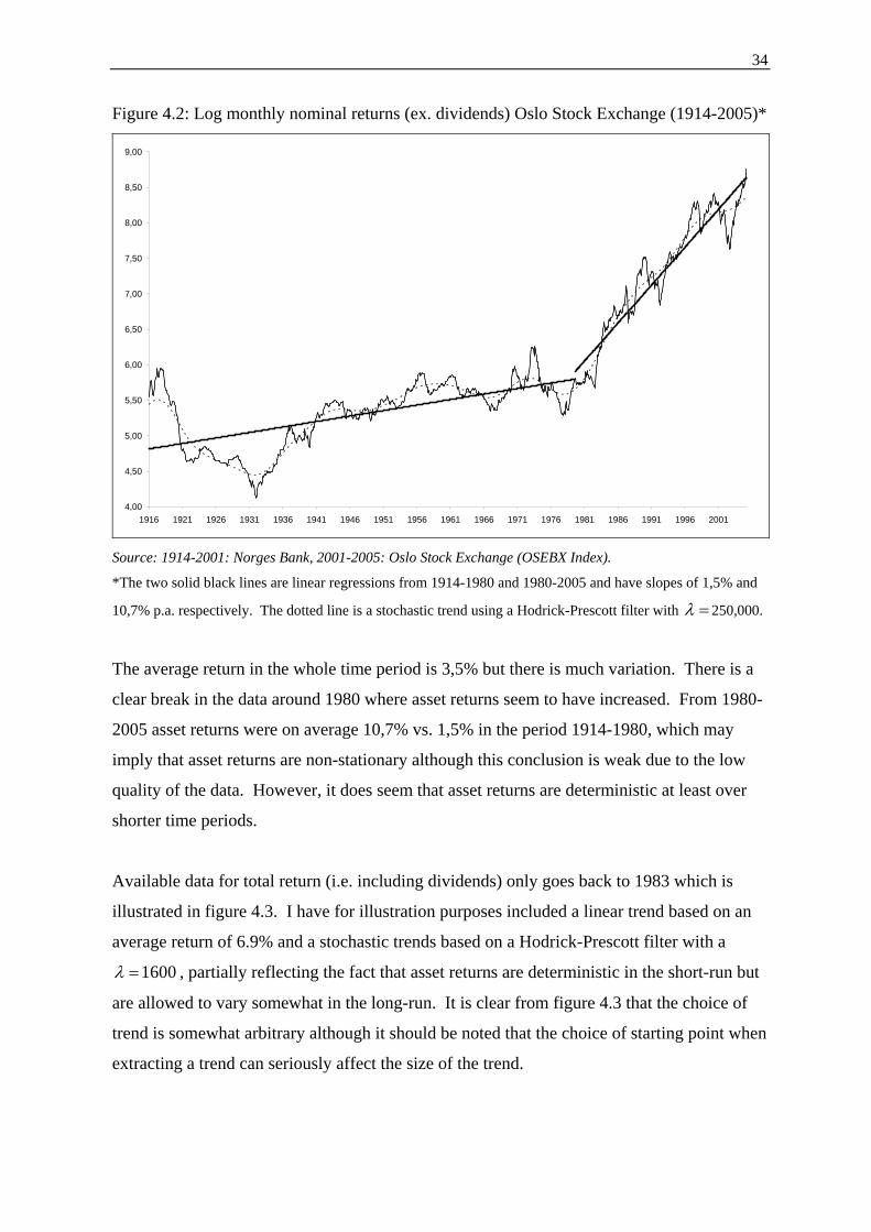
Figure 4.1: Price-to-book ratio Oslo Stock Exchange (1983-2005), quarterly*

0,0

0,5

1,0

1,5

2,0

2,5

3,0

1983 1985 1987 1989 1991 1993 1995 1997 1999 2001 2003 2005

Source: First Securities ASA.

*Excludes shipping and financial sectors. The series has been adjusted for changes in accounting and dividend

payout regimes. The dotted line represents the period average price-to-book ratio of 1.7x.

4.2.3 Deviation in asset returns from their long-term trend:

There is no logical inconsistency between a Tobin’s q approach to valuing the aggregate

asset market and the CAPM approach. Nor is there any logical inconsistency with an

alternative methodology proposed by Kaminsky & Reinhart (1999) and Borio & Lowe

(2002). They argue that one can identify asset price bubbles as deviations in asset return

from a non-stationary trend, although Borio & Lowe (2002)’s methodology emphasises

cumulative effects rather than period imbalances. Both implicitly assume that asset returns

are have a “trend level” which reflect investor expectations. This is not all that different

from the CAPM approach and the Tobin’s q approach as all three methodologies implicitly

assume that asset returns will be fairly stable over time and that deviations are likely to be

reversed since profits cannot grow faster than the economy as a whole in the steady state.

Borio & Lowe (2002) investigates whether above average growth in asset prices and credit

can serve as a useful indicator of financial crises. They use a Hodrick-Presocott filter on

asset returns and credit growth to estimate an “asset price-gap” and a “credit-gap”. Using

33

cross country annual data from 1960-1999 on a sample of OECD countries they find that

when using an asset return threshold of a cumulative increase of 40% above trend in

conjunction with a 4% credit growth gap, they can ex-ante predict all financial crisis

identified by Bordo et al. (2001). Their findings are remarkably robust despite failing to

account for real estate prices due to data limitations. Interestingly they find that investments

and the “investment gap” does not serve as a good predictor of financial crisis.

As argued by Allen & Gale (1999) financial distress usually succeeds asset price bubbles. It

is therefore reasonable to assume that an asset price bubble can occur when asset prices are

sufficiently higher than their long term trend. The size of this threshold is obviously open to

debate but one can get a general idea by using Borio & Lowe (2002)’s 40% threshold as a

starting point and examining empirical data for Norway.

Identifying financial crises in Norway is therefore a good place to start. Gerdrup (2003)

identifies three financial crises since end of the 19th century: 1899-1905, 1920-28 and 1988-

92. Gerdrup finds that the common denominators for these three periods of financial crisis

were significant bank expansion and banking competition, considerable asset price inflation

and increased indebtedness, and that they were followed by severe economic downturns.

Unfortunately, for the purposes of this analysis reliable asset return data only encompass the

financial crises in 1988-92.

The longest time series data on asset returns available in Norway is the Historical Stock

Price Indexes 1914-2001 from Norges Bank, as shown in figure 4.2. Unfortunately, it is

incomplete and hence not comparable over time for at least two reasons. First, prices are

nominal and second, and perhaps more importantly, dividends are ignored. Since dividends

payout regimes may vary over time this is a serious drawback and hence the time series

shown in figure 4.2 is clearly second best. However, I have included it for illustration

purposes as it illustrates well that the trend in asset returns varies somewhat over time.

34

Figure 4.2: Log monthly nominal returns (ex. dividends) Oslo Stock Exchange (1914-2005)*

4,00

4,50

5,00

5,50

6,00

6,50

7,00

7,50

8,00

8,50

9,00

1916 1921 1926 1931 1936 1941 1946 1951 1956 1961 1966 1971 1976 1981 1986 1991 1996 2001

Source: 1914-2001: Norges Bank, 2001-2005: Oslo Stock Exchange (OSEBX Index).

*The two solid black lines are linear regressions from 1914-1980 and 1980-2005 and have slopes of 1,5% and

10,7% p.a. respectively. The dotted line is a stochastic trend using a Hodrick-Prescott filter with λ = 250,000.

The average return in the whole time period is 3,5% but there is much variation. There is a

clear break in the data around 1980 where asset returns seem to have increased. From 1980-

2005 asset returns were on average 10,7% vs. 1,5% in the period 1914-1980, which may

imply that asset returns are non-stationary although this conclusion is weak due to the low

quality of the data. However, it does seem that asset returns are deterministic at least over

shorter time periods.

Available data for total return (i.e. including dividends) only goes back to 1983 which is

illustrated in figure 4.3. I have for illustration purposes included a linear trend based on an

average return of 6.9% and a stochastic trends based on a Hodrick-Prescott filter with a

1600λ = , partially reflecting the fact that asset returns are deterministic in the short-run but

are allowed to vary somewhat in the long-run. It is clear from figure 4.3 that the choice of

trend is somewhat arbitrary although it should be noted that the choice of starting point when

extracting a trend can seriously affect the size of the trend.

35

Figure 4.3: Log real quarterly average returns (including dividends) Oslo Stock Exchange

(1983-2005)*

3,00

3,50

4,00

4,50

5,00

5,50

6,00

1983 1985 1987 1989 1991 1993 1995 1997 1999 2001 2003 2005

Source: Oslo Stock Exchange (OSEBX and TOTX Index) and Statistics Norway.

* The solid black line represents a linear trend based on an average return of 6.9%and the dotted line is a

stochastic trend using a Hodrick-Prescott filter with λ = 1,600.

Following Borio & Lowe (2002) I define the “asset price gap” as the difference between the

observed asset price level and the trend asset price level. For simplicity I have chosen to use

a linear trend when deriving the asset price gap. An asset price gap based on a linear trend is

shown in figure 4.4. It is clear from figure 4.4, however, that the results are very similar to

that of the price-to-book ratio in figure 4.1 hence they are shown together in a standardized

framework in figure 4.5.

36

Figure 4.4: Asset price gap Oslo Stock Exchange (1983-2005)*

-80,0%

-70,0%

-60,0%

-50,0%

-40,0%

-30,0%

-20,0%

-10,0%

0,0%

10,0%

20,0%

30,0%

40,0%

50,0%

60,0%

70,0%

80,0%

1983 1985 1987 1989 1991 1993 1995 1997 1999 2001 2003 2005 * Based on the percentage difference between the log of real returns and a linear trend.

Figure 4.5: Asset price gaps compared: deviation from trend vs. price-to-book ratio*

-80,0%

-70,0%

-60,0%

-50,0%

-40,0%

-30,0%

-20,0%

-10,0%

0,0%

10,0%

20,0%

30,0%

40,0%

50,0%

60,0%

70,0%

80,0%

1983 1985 1987 1989 1991 1993 1995 1997 1999 2001 2003 2005

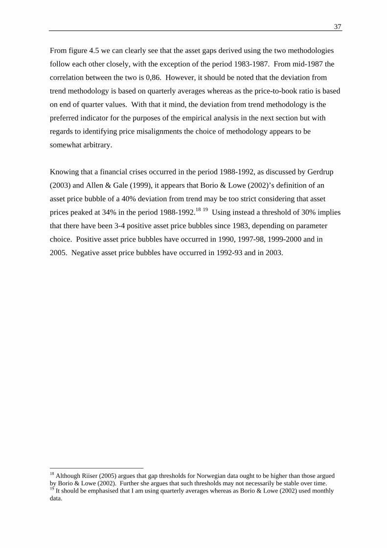
* The solid line is the asset price gap based on a linear trend and the dotted line is the percentage deviation in

the price-to-book ratio standardized to 1 around its periodic average of 1.70x.

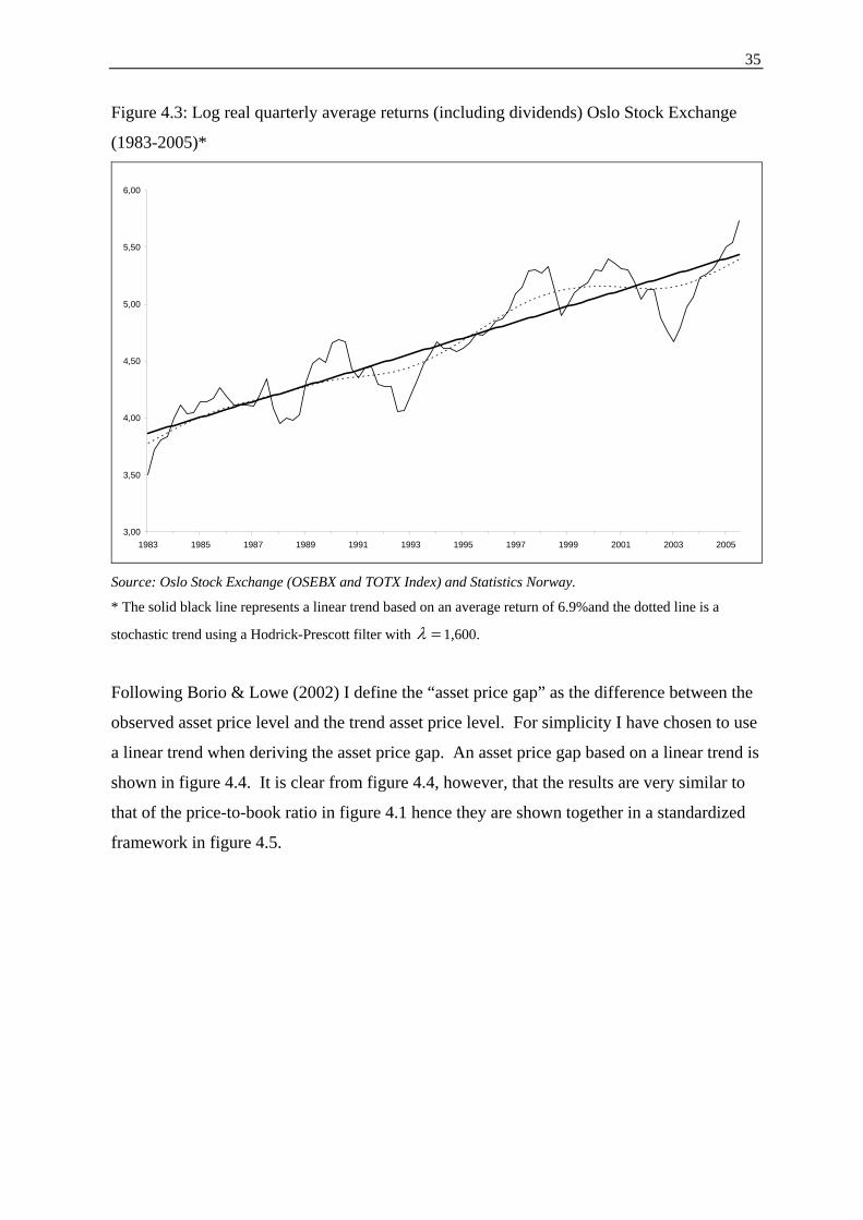
37

From figure 4.5 we can clearly see that the asset gaps derived using the two methodologies

follow each other closely, with the exception of the period 1983-1987. From mid-1987 the

correlation between the two is 0,86. However, it should be noted that the deviation from

trend methodology is based on quarterly averages whereas as the price-to-book ratio is based

on end of quarter values. With that it mind, the deviation from trend methodology is the

preferred indicator for the purposes of the empirical analysis in the next section but with

regards to identifying price misalignments the choice of methodology appears to be

somewhat arbitrary.

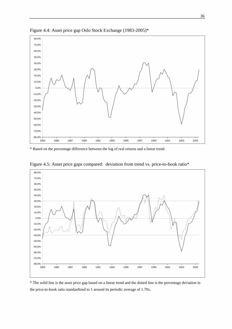
Knowing that a financial crises occurred in the period 1988-1992, as discussed by Gerdrup

(2003) and Allen & Gale (1999), it appears that Borio & Lowe (2002)’s definition of an

asset price bubble of a 40% deviation from trend may be too strict considering that asset

prices peaked at 34% in the period 1988-1992.18 19 Using instead a threshold of 30% implies

that there have been 3-4 positive asset price bubbles since 1983, depending on parameter

choice. Positive asset price bubbles have occurred in 1990, 1997-98, 1999-2000 and in

2005. Negative asset price bubbles have occurred in 1992-93 and in 2003.

18 Although Riiser (2005) argues that gap thresholds for Norwegian data ought to be higher than those argued by Borio & Lowe (2002). Further she argues that such thresholds may not necessarily be stable over time. 19 It should be emphasised that I am using quarterly averages whereas as Borio & Lowe (2002) used monthly data.

38

5. Empirical results EQUATION CHAPTER 1 SECTION 5 There have been relatively few studies on empirical interest rate rules on Norwegian data.

Arguably this is because Norges Bank has only pursued an inflation targeting policy since

2001 which limits data availability. Recent empirical literature on interest rate rules in

Norway includes Bernhardsen & Bårdsen (2004), Olsen et al. (2002) and Akram et al.

(2005). In addition, Norges Bank publishes various interest rate rules each quarter including

a standard Taylor rule, an Orphanides rule (see section 2.3), a weighted Taylor rule with

foreign interest rates and an estimated reaction function.20 These are shown relative to actual

interest rate setting in figure 5.1.

Figure 5.1: Interest rate rules versus actual interest rate (sight deposit rate)

0%

1%

2%

3%

4%

5%

6%

7%

8%

2000 2001 2002 2003 2004 2005 2006

Sight deposit rate

Taylor rule

Orphanides rule

Rule with foreigninterest rateReaction function

Source: Norges Bank Inflation Report No. 3, 2005.

In the next section I will first review some of the previous empirical evidence on interest rate

rules in Norway. Thereafter I will perform an empirical analysis on two different samples.

The first sample is from 1993 and the second is from 1999. The latter has been used as a

robustness check as it represents a different monetary policy regime and includes more

20 Based on the findings of Bernhardsen & Bårdsen (2004). See Norges Bank Inflation Report No. 3, 2004.

39

variables that are not available from 1993. The choice of sample is based on a trade-off

between the availability of a reasonably long time series and the presence of a reasonably

stable monetary policy regime. Although Norges Bank did not formally adopt an inflation

targeting policy until 2001, Bernhardsen & Bårdsen (2004) have estimated interest rate rules

from 1999 (when Norges Bank informally adopted an inflation targeting policy). However,

Olsen et al. (2002) argues that monetary policy can be viewed as adhering to a Taylor rule

from as early as 1993. The two samples therefore provide insight into interest setting

behaviour in what can be viewed as two different monetary policy regimes.

Since a long time series may in general provide more robust results, I will first estimate an

empirical interest rate rule with data going back to 1993 and compare the results with the

previous empirical evidence. Second, with the same sample I will estimate a simultaneous

model with asset prices and see how asset prices can improve the empirical results. Third, I

will perform the same analysis on data from 1999 as a check for robustness.

5.1 Previous empirical evidence Bernhardsen & Bårdsen (2004) find that the empirical interest rate rule that best describe the

interest rate setting of Norges Bank in the period 1999-2004 is a variant of the Orphanides

rule with the estimated growth gap (for the following 12 months) instead of the actual

growth gap. In addition, they use expected inflation similar to the findings of Clarida et al.

(1999) and add the wage growth gap and the foreign interest rate to increase the explanatory

power of the model. They use the latter as an instrumental variable for exchange rate effects

to avoid the simultaneity problem. I have updated their analysis through Q3 2005 and found

the following results (t-values in parenthesis):21

(5.1) 1 1 1(10,29) (2,13) (2,80) (1,47) (2,84)0,8 0, 2[1,5 1,0 1,0 0,9 ]t t t t t t t ti i E E g ui wπ− + += + + + +

where i is the sight deposit rate, 1t tE π + is expected inflation, 1t tE g + is estimated 12 month

GDP growth rate, ui is the foreign interest rate and w is wage growth. The model is

constrained to have a coefficient equal to zero since all variables are measured as deviations

from their steady state (see Appendix 1 for a complete description of all the variables). That

is, when all explanatory variables are in their steady states (i.e. all gaps are equal to zero) the 21 The original findings by Bernhardsen & Bårdsen (2004) are largely the same.

40

interest rate gap is also zero, which in this case implies a steady state nominal interest rate of

5,5%.

The results have some interesting implications. First the coefficient on the lagged interest

rate is high relative to the other explanatory variables. In isolation this is not problematic

since the lagged interest rate is included to emulate interest rate smoothing. However, one

cannot rule out that other explanatory variables can have been omitted. Second, all variables

are significant under traditional standards and enter the rule with the correct sign, except the

foreign interest rate gap. The inclusion of the latter reflects an emphasis on a priori

expectations and limited data availability.

Olsen et al. (2002) attempts at finding other real time variables that can substitute for the

output gap or the growth gap. They find that the unemployment gap or the wage gap in

combination with the credit growth may yield satisfactory explanatory results.22 Their study

is also based on a longer time series than Bernhardsen & Bårdsen as they find that interest

rate setting in Norway follows a Taylor rule from as early as 1995 despite Norges Bank not

having adopted a formal inflation target until 2001. In that respect their findings can be

viewed as more robust than those of Bernhardsen & Bårdsen.

Akram et al. (2005) does not attempt at estimating empirical interest rate rules, but instead

simulates relative economic performance of a large general equilibrium model under various

policy rules. Similarly to Taylor (2001) they find that adding exchange rates to a simple

policy rule actually does more harm than good as output variability increases. However,

they find that adding asset prices as an explanatory variable may be beneficial as it reduces

output variability. Although this particular study is based on simulation and does not

attempt at measuring the behavioural pattern of Norges Bank, their findings provide a

justification for adding asset prices to an interest rate rule following many of the arguments

in section 3.

22 However, Bernhardsen & Bårdesen (2004) finds that the unemployment gap is not significant on Norwegian data, although only in conjunction with other measures of relative economic performance.

41

5.2 Data and methodology In estimating empirical interest rate rules for Norges Bank (with or without asset prices) I

have opted to follow Bernhardsen & Bårdsen (2004) in the sense that I have focused mainly

on a priori expectations of the signs of the coefficients and less so on the level of

significance. This is mainly due to a limited sample size although I have opted to use data

from 1993 which increases the sample. Olsen et al. (2002) estimates interest rate rules from

1995 arguing that interest setting from 1995 follows closely to a Taylor rule. Bjørnland

(2005b) uses a similar argument with data going back to 1993, with the exception of the

period from the fourth quarter of 1996 through the first quarter of 1998 (i.e. 6 observations)

when Norges Bank clearly was preoccupied with defending the Norwegian krone. I have

used a dummy variable to exclude this time period. Nevertheless, the sample size is still

relatively small and a priori expectations should still be emphasised. A complete description

of the dataset is provided in Appendix 1. Unit root tests (see Appendix 1) confirm that all

variables are non-stationary in the levels, thereby motivating me to take differences or

analysing the variables as deviations form trend (gap). For some variables like the (domestic

and foreign) interest rate and inflation, the variables are close to rejecting the unit root

hypothesis. Due to the low power of the unit root test in small samples, I have decided to

treat these variables as stationary, modelling them in the levels.

Two points about model specification has to be made. First, I have constrained all models to

have an intercept equal to zero by measuring all variables as deviations from their steady

states. This is possible since all non-stationary variables have been detrended using a

Hodrick-Prescot filter. Second, I have added an interest rate lag variable in all models to

emulate interest rate “smoothing” similar to the forward looking rule from Clarida et al.

(1999) (see equation (2.8)). Both of these points are important for interpretation. Avoiding

an intercept term is advantageous for three reasons. First, model misspecification and

exclusion of potentially important variables will show up in the coefficient for the interest

smoothing parameter. All things equal, one would prefer a policy rule with a low coefficient

over one with a high coefficient on the lagged interest rate. Second, avoiding an intercept

term makes it easier to allow for a time-varying inflation target since, as mentioned in

section 2.3, the intercept can be interpreted as the steady state real interest rate plus the

42

inflation target.23 Third, it makes it easier to include an asset price gap as a deviation from

fundamental value (more on this will be discussed in section 5.4).

5.3 Interest rate rules in Norway from 1993 With data from 1993, I do not have access to all the variables used by Bernhardsen &

Bårdsen (2004). However, I can estimate more traditional interest rate rules similar to those

of Taylor (1993) and Orphanides (2000). In general, however, Taylor rules and Orphanides

rules from 1993 and from 1999 generate equally unsatisfactory results. That is, neither

output nor growth are significant in the empirical interest rate rule. The following OLS

results for an empirical Taylor rule and empirical Orphanides rule with data from 1993

illustrates this:24

(5.2) 1(11,41) (5,75) (0,80)0,68 0,32[2,04 0, 21 ]t t t ti i yπ−= + +

1(10,77) (6,89) (0,24)0,67 0,33[2,09 0,04 ]t t t ti i gπ−= + +

Note that y is the output gap and g is the ex-post growth gap (as defined in Appendix 1). It

should also be noted that the above equations use actual inflation as opposed to expected

inflation as argued by Clarida et al. (1999).

The lack of significance of the output gap and the growth gap may explain some of the

motivation by Bernhardsen & Bårdsen (2004) for using the expected growth gap instead of

the ex-post growth gap as in (5.2). The coefficient on the lagged interest rate is fairly high

albeit lower than in (5.1), which in isolation is a good thing. In that sense, it may appear that

interest rate smoothing is less important with longer time series, which is consistent with the

empirical findings in the U.S. (see e.g. Taylor (1993)).

However, the relatively low t-values for the output gap and the growth gap indicate that an

empirical interest rate rule is best described with inflation as the only explanatory variable.

However, there are theoretical problems with such a formulation since, as discussed in

section 2.1, monetary policy is a trade-off between inflation and output stabilisation. Hence,

a priori expectations tell us that an interest rate rule with inflation as the only explanatory 23 This follows Bernhardsen & Bårdsen (2004) whom have used a 2% inflation target up to Q1 2001. 24 Dummy variable for regime change is excluded for presentation purposes.

43

variable is an insufficient description of Norges Bank’s reaction function since it ignores

output stabilisation.

One alternative solution could be to add the unemployment gap as an alternative real time

variable, as argued by Olsen et al. (2002). Adding the unemployment gap (instead of the

growth gap) to the Orphanides rule in (5.2) yields the following results:

(5.3) 1(13,56) (6,37) ( 2,37)0,68 0,32[1,95 0,51 ]t t t ti i uπ−

−= + −

Here the unemployment gap enters the rule with the correct sign (sine unemployment is

counter cyclical) and is significant under traditional standards.25 Hence the best available

empirical interest rate rule from 1993 is an interest rate rule with inflation and

unemployment as the explanatory variables. This is in line with the findings of Olsen et al.

(2002), but clearly ignores some potentially important variables as shown by Bernhardsen &

Bårdsen (2004). Equation (5.3) is, however, a reasonable starting point for a simultaneous

model with asset prices.26

5.4 Asset prices in a simultaneous model from 1993 Adding asset prices outright to equation (5.3) will yield inconsistent estimators of the

coefficients since asset prices may be an endogenous variable. A Wu-Hausman test for

endogeneity confirms that this in fact is the case as shown in Appendix 1. Instead, as argued

section 3, it might be plausible to formulate an interest rate rule with asset prices in a

simultaneous model:

(5.4) 1 1 2 3 6 1,t t t t t ti i u aβ β π β β ε−= + + + +

(5.5) 1 1 2 2,t t t ta a iα α ε−= + +

Equation (5.4) is follows the findings from section 5.3 where a is the asset price gap, and 1ε

is an error term. Equation (5.5) explains the endogenous behaviour of the asset price gap

using lags and interest rates only ( 2ε is an error term). Although equation (5.5) could be

more elaborate I have attempted at leaving it as simple as possible to avoid complicating the

25 Similar results are found by adding the unemployment gap to the Taylor rule in (5.2). 26 Note however that I have not included the foreign interest rate gap as argued by Bernhardsen & Bårdsen (2004) mainly due to simplicity (but also due to its limited marginal effect).

44

problem further. That is, I am not ruling out that there may be other potentially important

explanatory variables for the behaviour of asset prices but these will be included in the

lagged endogenous variable.

I would expect all the coefficients in equation (5.4) to be positive and that 10 1β< < . This

implies that high asset prices in isolation imply high interest rates and vice versa. A

coefficient of 1β less than unity is important to ensure stability of the model. The same

applies to equation (5.5) where 10 1α< < to maintain stability. Further, I would expect

2 0α < since higher interest rates in isolation would lead to lower asset prices and vice versa.

I have used two stage least squares (2SLS) to estimate the model above. There are three

reasons for this. First, it is a fairly simple and intuitive methodology which is easily

interpretable. Second, an instrumental variable approach can be ruled out due to lack of

readily available and good instrumental variables. Third, indirect least squares is not

applicable since the system is over-identified.27 In addition, 2SLS is generally though of as

possessing better small sample properties than other similar estimators.

Applying 2SLS on equations (5.4) and (5.5) yield the following results:

(5.6) 1(10,88) ( 1,74) (2,04)(2,94)

ˆ ˆ0,79 0,21[1,97 0,56 0,06 ]t t t t ti i u aπ−−

= + − +

(5.7) 1(15,85) ( 3,00)

ˆ ˆˆ 0,90 2,15t t ta a i−−

= −

where a is the estimated asset price gap and i is the estimated interest rate gap found by

estimating the reduced form equations of the model. The asset price gap enters the model

with the correct sign and is significantly different from zero under traditional standards.

This may suggest that the asset price gap has important explanatory effects on the interest

rate setting behaviour of Norges Bank.

27 The system is overidentified since there are fewer exogenous variables in equation (5.5) (i.e. 1) than there are endogenous variables in the system (i.e. 2).

45

The same applies to inflation as its partial effect remains virtually unchanged. The

unemployment gap, however, is not significant by traditional standards but is kept in the

model due to a priori expectations.

The data from 1993 seems therefore to confirm the hypothesis that asset prices may be

useful as an information variable. A 1% overvaluation in asset prices increases interest rates

by 6 basis points and conversely a 1% increase in interest rates reduces asset prices by

2,15%, based on quarterly averages. This is qualitatively consistent with the findings by

Bjørnland & Leitemo (2005), although not quantitatively (since I measure effects on

quarterly averages and do not attempt to differentiate between short and long-term effects).

Moreover, the results indicate that the asset price gap is a more useful indicator for future

inflation than the ex-post growth gap and the ex-post output gap. However, more analysis is

needed to make similar conclusions about other potentially important variables that are

available in the 1999 sample.

5.5 Robustness check with data from 1999 The sample from 1999 is based on a different monetary regime than the sample from 1993.

Hence performing the same analysis as in section 5.3 and 5.4 on data from 1999 will give an

indication of the robustness of the results from the previous section. Furthermore, with the

results of Bernhardsen & Bårdsen (2004) in mind, it is clear that the results in section 5.3

omit some important explanatory variables such as expected inflation, the expected growth

gap, the foreign interest rate level and the wage growth gap. It would therefore be

interesting to check whether the methodology used in section 5.4 applied on data from 1999

will yield similar results.

I have formulated a model similarly to equations (5.6) and (5.7) but substituted (5.6) with the

results of Bernhardsen & Bårdsen in equation (5.1) and added the asset price gap. The

results using 2SLS are as follows:

(5.8) 1 1 1(6,06) (1,03) (2,56) (0,53) (2,84) (0,81)

ˆ ˆ0,90 0,10[2,09 2,66 0,99 1,77 0,05 ]t t t t t t t t ti i E E g ui w aπ− + += + + + + +

(5.9) 1(13,14) ( 3,20)

ˆ ˆˆ 1,00 2,69t t ta a i−−

= −

46

It is clear that all the variables enter the interest rate rule with the correct sign. Some of the

variables are not significantly different from zero, at least according to traditional standards.

The asset price gap has a coefficient of 0,05 which is relatively low regardless of whether it

is significantly different from zero or not, and is the variable with the least effect on interest

rates. Nevertheless, the asset price gap is clearly not significantly different from zero but I

will leave it in the model due to a priori expectations.

Another interesting observation is that inflation is no longer significant, which may suggest

that asset prices may contain information about future inflation. It may therefore be

interesting to repeat the analysis without the inflation gap. The results are as follows.

(5.10) 1 1(14,85) (5,05) (0,64) (2,52) (1,78)

ˆ ˆ1,03 0,33 0,12 0,14 0,01t t t t t t ti i E g ui w a− += + + + +

(5.11) 1(13,20) ( 3,24)

ˆ ˆˆ 1,00 2,72t t ta a i−−

= −

The asset price gap again enters with the correct sign and has a reasonably high significance

level, at least for the purposes of this analysis. Hence equation (5.10) describes interest rate

setting in Norway fairly well and indicates that asset prices contains information about future

inflation not found elsewhere. However, (5.10) has one major fault. The coefficient on the

lagged interest rate is higher than unity, which contradicts much of the empirical work on

interest rate rules. The coefficient on the lagged asset price gap in equation (5.11) is also

higher than unity although it has not changed much from (5.9). There are at least two

possible explanations for the high coefficient on the lagged variables. Either the explanatory

variables are in fact not very relevant or the endogenous variables are non-stationary. As

shown in Appendix 1 this may be the case for the lagged interest rate but certainly not the

case the asset price gap which clearly does not have a unit root. A more probable conclusion

is that the exogenous variables are not relevant enough due to the relatively small sample

size.

When comparing these results with those from section 5.4, one can draw at least four

conclusions. First, the results confirm in many ways the results from the sample from 1993.

The data from 1999 indicate that the asset price gap may be significant but that the marginal

effect on interest rates is small. Third, with data from 1999 and excluding inflation, equation

47

(5.10) indicates that asset prices contain information about future inflation not found

elsewhere. It should be noted, however, that the same dataset also confirms that there might

have been a misspecification problem in equation (5.6) since some potentially important

variables may have been omitted.

48

6. Conclusion The purpose of this thesis has been to survey and investigate the role of asset prices, in

particular stock prices, on monetary policy in Norway. I have found that although there has

been a long established consensus in the literature that asset prices should not be targeted

explicitly, recent literary contributions have argued that asset prices may contain information

regarding future inflation not found elsewhere, mainly due to their forward looking nature.

Other reasons include the existence of imperfect asset markets and severe asset price

misalignments (e.g. asset price bubbles), among others.

There exist several empirical contributions on asset prices and monetary policy. Generally

the literature has focused on measuring the relative efficiency of interest rate rules with asset

prices using calibrated small structural (New Keynesian) models (see e.g. Bernanke &

Gertler (2001)). Empirically estimated interest rate rules (reaction functions) that

incorporate asset prices have received relatively little attention (one notable exception is

Chadha et al. (2003)). One reason for this is the existence a simultaneity problem between

asset prices and interest rates making the identification issue problematic. Another is the

measurement problem associated with identifying asset price misalignments.

However, asset prices could be included in empirically estimated interest rate rules provided

the simultaneity and measurement problems are appropriately addressed. To avoid the

simultaneity problem I have formulated a simultaneous interest rate rule model where asset

prices enter endogenously. In measuring asset price misalignments I have opted to follow

the methodology used by Borio & Lowe (2002) which is based on measuring the asset price

gap as the deviation in cumulative asset returns from trend. I find that this methodology is

consistent with other asset price determination methodologies.

Using Norwegian data from 1993, I find that asset prices enter significantly in a

simultaneous model estimated using two stage least squares (2SLS). I also find that asset

prices contain more precise information on future inflation than the output gap and the

growth gap, particularly in conjunction with the unemployment gap. This implies that asset

49

prices can be viewed as an alternative real-time variable to the output gap or alike. These

results are supported using more recent data from 1999.

It is worth mentioning, however, that the modeling framework I have used does not

incorporate the short and long-term effects of asset price misalignments (as opposed to the

SVAR approach by Bjørnland & Leitemo (2005)). It follows therefore that the qualitative

results of the analysis in this paper may be correct but that the quantitative results may differ.

Furthermore, given the limited data available and relatively short time horizon of the

analysis, more research is needed to ascertain the relative usefulness of asset prices in

monetary policy.

50

References/Literature Akram, Q. F., G. Bårdsen and Ø. Eitrheim (2005): "Monetary policy and asset prices: to respond or not?",

Norges Bank Working Paper

Allen, Franklin & Douglas Gale (1999): "Bubbles, crises and policy", Oxford Review of Economic Policy, Vol. 15, No. 3

llen, Franklin & Douglas Gale (2000a): "Asset price bubbles and monetary policy", Stockholm: Sveriges Riksbank-Stockholm School of Economics Conference on "Asset Markets and Monetary Policy", June 16-17,2000.

llen, Franklin & Douglas Gale (2000b): "Comparing Financial Systems", MIT Press

Arnold, Lutz. G. (2002); “Business cycle theory”, Oxford Universtiy Press

Ball, L. (1999): “Policy rules for open economies”, in John B. Taylor, ed., “Monetary policy rules”, University of Chicago Press, p. 127-144.

Barro R.J. & D.B. Gordon(1983): “Rules, discretion and reuptation in a model of monetary policy”, Journal of Monetary Economics, 12(1), p. 101-121

Bean, C. (2003): "Asset prices, financial imbalances and monetary policy: Are inflation targets enough?", Reserve Bank of Australia, RBA Annual Conference, Volume 04

Bernanke, Ben & Allan S. Blinder (1988): ”Credit , money and aggregate demand”, American Economic Review, 78, p. 435-9

Bernanke, Ben & Mark. Gertler (1989): "Agency costs, net worth and business fluctuations", American Economic Review, 79 (1), pp 14-31

Bernanke, Ben & Mark. Gertler (1999): "Monetary policy and asset volatility", Federal Reserve Bank of Kansas City Economic Review, 84 (4), pp. 17-52

Bernanke, Ben & Mark. Gertler (2001): "Should central banks respond to asset prices", American Economic Review, 91 (2), pp.253-57.

Bernanke, Ben & Kenneth N. Kuttner (2004): “What explans the stock market’s reaction to Federal Reserve policy?”, NBER Working Paper No. 10402

Bernanke, Ben & I. Mihov (1998): ”Measuring monetary policy” Quarterly Journal of Economics, 113(3), p. 869-902

Bernhardsen, Tom. & Gunnar Bårdsen (2004): "Sammenhengen mellom styringsrenten og makroøkonomiske variable: Noen enkle ligninger for Norge", Norges Bank Staff Memo

Bernhardsen, T.; Ø. Eitrheim; A.S. Jore; Ø. Røisland (2004): " Real-time Data for Norway: Challenges for Monetary Policy", Discussion Paper 26/2004, Deutsche Bundesbank.

Bjørnland, Hilde (2005a): ” Pengepolitikk i praksis. Fakta og fiksjon”, Presentation at the Autumn Conference for Samfunnsøkonomisk forening, Nov. 2005

Bjørnland, Hilde (2005b): "Monetary Policy and Exchange Rate Interactions in a Small Open Economy," Norges Bank Working Paper 2005/16.

51

Bjørnland, Hilde; Leif Brubakk & Anne Sofie Jore (2004): "Produksjonsgapet i Norge – en sammenlikning av metoder", Penger og Kreditt 4/2004, Norges Bank

Bjørnland, Hilde & Kai Leitemo. (2005): "Identifying the interdependence between US monetary policy and the stock market", Working paper, University of Oslo

Bordo, M.; D. Klingebiel & M.S. Martinez-Peria (2001): "Financial Crises: lessons from the last 120 years.", Economic Policy, April 2001

Bordo, Michael D. & Olivier Jeanne (2002): "Boom-busts in asset prices, economic stability and monetary policy", NBER Working Paper No. 8966

Borio, Claudio & Philip Lowe (2002): "Asset prices, financial and monetary stability: exploring the nexus", BIS Working Paper No. 114.

Borio, C.; N. Kennedy & S. Prowse, (1994): “Exploring aggregate asset price fluctuations across countries: measurement, determinants and monetary policy implications”, BIS Economic Papers, No. 40, Basel, April 1994.

Brainard, William C. (1969): “Uncertainty and the effectiveness of policy” American Economic Review, 57, p. 411-425.

Carlstrom, Charles T. & Timothy S. Fuerst, (2001): "Monetary policy and asset prices with imperfect credit markets", Federal Reserve Bank of Cleveland Economic Review, 37 (4), p. 51-59.

Cecchetti, Stephen; Hans Genberg, John Lipsky & Sushil Wadhwani (2000): "Asset prices and central bank policy", London: International Center for Monetary and Banking Studies

Chadha, Jagjit S.; Lucio Sarno & Giorgio Valente, (2003): "Monetary policy rules, asset prices and exchange rates.", Centre for Economic Policy Research, Discussion Paper No. 4114

Chirinko, R. (1993): “Business fixed investment spending: A critical survey of modeling strategies, empirical results and policy implications”, Journal of Economic Literature, 31 (1), p.1875-1911

Christiano, L.J.; M. Echenbaum & C. Evans (2001): ”Nominal rigidities and the dynamic effects of a shock to monetary policy”, NBER Working Paper No. 8403, July 2001

Clarida,Richard; Jordi Gali & Mark Gertler (1999): "The science of monetary policy: A New Keynesian perspective", Journal of Economic Litterature, December 1999

Diamond, Douglas (1991): "Monitoring and reputation: the choice between bank loans and directly placed debt", Journal of Political Economy, August 1991

Dotsey, M. & R.G. King (2001): “Pricing, production and persistence”, NBER Working Paper No. 8407, August 2001

Fuhrer, J.C. & G.R. Moore (1995): “Inflation persistence”, Quarterly Journal of Economics, 110 (1), p. 127-159

Gerdrup, Karsten R. (2003): "Three episodes of financial fragility in Norway since the 1890s.", BIS Working Paper No. 142

Gordon M.J. (1962): ”The investment, financing and valuation of the corporation”, Irwin, Homewood, Il.

Gurkaynak, R. S. (2005): "Econometric tests of asset price bubbles: taking stock", Finance and Economics Discussion Serires, Federal Reserve Board, Washington, D.C., April 2005.

Hall, R. (2000): “e-capital: the link between the stock market and the labour market in the 1990s”, Brookings Papers on Economic Activity, 2000.

52

Hansen, J. (2003): "Financial cycles and bankruptcies in the Nordic countries", Sveriges Riksbank Working Paper Series No. 149

Hubbard, G. (1998): “Capital market imperfections and investment”, Journal of Economic Literature, 36 (1), p. 193-225

International Monetary Fund (2000): "Asset prices and business cycles", IMF World Economic Outlook 2000, Chapter 3.

Kaminsky & Reinhart (1999): ”The twin crises: the causes of banking and balance-of-payments problems”, American Economic Review, Vol. 89, No 3, June, p. 473-500

Klovland, J.T.(2004). "Historical stock price indices in Norway 1914-2001", 329-348, Chapter 8 in Eitrheim, Ø., J.T. Klovland and J.F. Qvigstad (eds.), Historical Monetary Statistics for Norway 1819-2003, Norges Bank Occasional Papers no. 35, Oslo, 2004

Lansing K.J. (2002): “Real-time estimation of trend output and the illusion of interest rate smoothing”, Federal Reserve Bank of San Francisco Economic Review 2002, 17-34

Norges Bank’s Inflation Report No. 3, 2004

Norges Bank’s Inflation Report No. 1, 2003

Malkiel, B. M. (2003): "The efficient market hypothesis and its critics.", Journal of Economic Perspectives, Vol. 17, No. 1

Mankiw (1986): “The allocation of credit and financial collapse”, Quarterly Journal of Economics 101, Aug. 1986, p. 455-470

McCallum, B.T. (1999): “Issues in the design og monetary policy rules”, in J. Taylor and M. Woodfrod (eds.), Handbook of Macroeconomics, Vol 1C, Amsterdam: Elsevier North-Holland, p. 1483-1530

McCallum B.T. & E. Nelson (1999): “An optimizing IS-LM specification for monetary policy and business cycle analysis”, Journal of Money, Credit, and Banking, 31(3), part 1, August 1999, p. 296-316

Obstfeldt, M. & K.Rogoff (1995): “The mirage of fixed exchange rates”, Journal of Economic Perspectives”, 9 (4), p. 73-96.

Olsen, Kjetil; Jan Fredrik Qvigstad & Øistein Røisland (2002): "Monetary policy in real time: the role of simple rules.", Paper prepared for BIS Autum Economist's Meeting, October 2002.

Orphanides, A., R. Porter, D. Reifschneider, R. Tetlow and F. Finan (2000): "Errors in the measurement of the output gap and the design of monetary policy", Journal of Economics and Business, 52, 117-141.

Poole, W. (1979): “Optimal choice of monetary policy instruments in a simple stochastic macro model”, Quarterly Journal of Economics, 84 (2), p. 197-216

Rigobon R. & B. Sack (2003): “Measuring the reaction of monetary polic to the stock market”, The Quarterly Journal of Economics, 118 (2), p. 639-639

Rigobon R. & B. Sack (2004): “The impact of monetary policy on asset prices”, Journal of Monetary Policy, 51, p. 1553-1575.

Riiser, Magdalena D. (2005): “Boligpriser, aksjekurser, investeringer og kreditt – hva sier de om bankkriser? En historisk analyse på norske data”, Penger og Kreditt 2/2005, Norges Bank

Robertson, D. and S. Wright. (2002): "What does q predict?",Unpublished

Robertson, D. and S. Wright. (2003): "The good news and the bad news about long-run stock returns", Unpublished

53

Roll, R. (1977): "A critique of the asse pricing theory's tests. Part I: On past and potential testability of the theory.", Journal of Financial Economics, No. 4, 1977.

Rudebusch, G.D. (2002): “Term structure evidence on interest rate smoothing and monetary policy intertia”, The Economic Journal, 112(479), p. 402-432

Sargent, T. J. & N. Wallace (1975): “Rational expectations, the optimal monetary instrument, and the optimal money supply rule”, Journal of Political Economy, 83(2), April 1975, p. 241-254

Shiller, R. J. (2003): "From efficient markets theory to behavioural finance.", Journal of Economic Perspectives, Vol. 17, No. 1

Smithers, A. and S. Wright. (2000): "Valuing Wall Street: Protecting wealth in turbulent markets", McGraw-Hill

Stiglitz, J. & A. Weiss (1981): “Credit rationing in markets with imperfect information”, American Economic Review, 71 (3), 1981

Svensson, Lars E. O. (2000): “Open-economy inflation targeting”, Journal of International Economics, Febr. 2000, 50 (1), p. 117-153.

Taylor, John B. (1993): “Discretion versus policy rules in practice”, Carnegie-Rochester Conference Series on Public Policy 39, Elsevier Science Publishers B.V., p. 195-214

Taylor, John B. (1999): "Monetary policy rules", The University of Chicago Press, Chicago and London

Taylor, John B. (2001): "The role of the exchange rate in monetary-policy rules", The American Economic Review, Vol. 91

Tobin, John. (1969): "A general equilibrium approach to monetary theory.", Journal of Money, Credit and Banking, Vol 1, pp 15-29

Walsh, Carl E. (2003): “Monetary theory and policy”, The MIT press

Woodford, M. (2001): “Inflation stabilisation and welfare”, NBER Working Paper No. 8071, Jan. 2001

54

Appendix 1: Data description and unit root tests I have used two data samples to test for the significance of asset prices in interest rate rules.

The first sample is from 1993 and the second is from 1999. The latter has been used as a

robustness check as it represents a different monetary policy regime and includes more

variables that are not available from 1993.* The data variables are as follows:

i Sight deposit rate less its steady state level. The steady state nominal interest rate is

assumed to be 5,5%.* The data is calculated as quarterly averages based on daily data

from Q1 1991 to Q3 2005. Source: Norges Bank

π Inflation measured by KPI-JAE less the inflation target. The inflation target is

assumed to be 2% prior to Q2 2001 and 2.5% thereafter.* The series is calculated

from Q1 1993. Source: Statistics Norway

y Output gap as measured by seasonally adjusted quarterly mainland GDP less potential

output. Potential output is estimated using a Hodrick-Prescott filter with 1600λ =

based on data from Q1 1978 to Q2 2005. Source: Statistics Norway

g The growth gap as measured by actual growth in mainland GDP less steady state

growth. Steady state growth is assumed to be 2.5% throughout the period.*

u Unemployment gap as measured by seasonally adjusted unemployment less its steady

state level. The steady state unemployment level is assumed to be 4,5% throughout

the sample period (based on the period average). The data series is based on data from

Q1 1989 to Q3 2005. Source: Statistics Norway

a Asset price gap as measured by the deviation in cumulative asset returns from a linear

trend calculated using quarterly averages. The data series is based on the OSEBX and

TOTX indexes from Q1 1983 to Q3 2005. Source: Oslo Stock Exchange.

pb Weighted average price-to-book ratio for all non-financial and non-shipping

companies on the Oslo Stock Exchange. The data series is based on end of quarter

data from Q1 1983 to Q2 2005. Source: First Securities ASA

* See Bernhardsen & Bårdsen (2004).

55

1t tE π + Estimated inflation for the next 12 months less the inflation target. The inflation target

is assumed to be 2% prior to Q2 2001 and 2.5% thereafter.* The data series is based

on data from Q1 1999 to Q3 2005. Source: Norges Bank.

1t tE g + Estimated growth gap for the next 12 months. Steady state growth is assumed to be

2,5%.* The data series is based on data from Q1 1999 to Q3 2005. Source: Norges

Bank.

ui Foreign interest rate gap (trading partner weighted). Steady state foreign interest rate

is assumed to be 3,5%.* The data series is based on data from Q1 1999 to Q3 2005.

Source: Norges Bank.

w Wage growth gap. Steady state wage growth is assumed to be 4,75%.* The data

series is based on data from Q1 1999 to Q3 2005. Source: Norges Bank.

Unit root tests results using the Augmented Dickey Fuller test for the data set are as follows:

Table A1.1: Augmented Dickey Fuller test results (based on level variable where appropriate)

t-adf Variable Data period Lags: 1 Lags: 2 Lags: 3 Lags: 4i Q2:1992 - Q3:2005 -3,00 -2,59 -2,75 -2,48 π Q2:1994 - Q3:2005 -1,72 -2,17 -2,02 -1,40 y 1 Q2:1979 – Q2:2005 -1,28 -1,44 -1,56 -1,94 u 1 Q2:1990 - Q3:2005 -0,49 -0,75 -1,08 -1,10 a Q1:1983 - Q3:2005 -3,15 2 -2,77 -3,52 2 -3,25 2

1t tE π + Q1:1999 – Q3:2005 -1,89 -2,52 -2,78 -1,90 ui Q1:1999 – Q3:2005 -2,65 -2,87 -3,24 -2,78 w Q1:1999 – Q3:2005 -2,96 -3,01 -2,78 -2,02

1. Based on the level variable (i.e. not first differences or gaps)

2. Indicates that the t-adf value is greater than the relevant critical value with 5% significance.

With a 5% significance level only the asset price gap shows signs of not having a unit root.

* See Bernhardsen & Bårdsen (2004).

56

Appendix 2: Endogeneity test for asset prices To test for the endogeneity of the asset price gap in an interest rate rule framework I have

used a Wu-Hausman test using data from 1993.

The structural form equations of the model are:

(5.12) tttttt vauii ++++= − 43211 ββπββ

(5.13) tttt wiaa ++= − 211 αα

In reduced form:

(5.14) tttttt auii ,11141312111 επ +Π+Π+Π+Π= −−

(5.15) tttttt auia ,21242322121 επ +Π+Π+Π+Π= −−

Assume that there is a linear relationship between tv and 2,tε given by:

(5.16) ttt ev += ,2ρε

This is plausible since 2,tε is given by:

42

2,2 1 βα

αε−

+= tt

twv ⇔

4342143421te

ttt wv )(11

2,2

2

42 −+−

=α

εα

βα

ρ

Combining (5.12) and (5.16) gives:

(5.17) ttttttt eauii +++++= − ,243211 ρεββπββ

If 0ρ ≠ then a is endogenous.

OLS results on (5.17) are:

(5.18) 1 2,(15,04) (4,07) ( 2,41) (2,82) ( 6,80)

ˆ 0,79 0,41 0,12 0,01 0,04t t t t t ti i u aπ ε−− −

= + − + −

Since the t-value for the coefficient of 2ε is -6,80 one can conclude that ρ is significantly

different from zero and that ta is endogenous. More formally, we reject the null hypothesis

of exogeneity. Further, since 0ρ < , the coefficient on asset prices in a one equation interest

rate rule will be underestimated.

57

This result is confirmed using data from 1999 and using the interest rate rule formulation by

Bernhardsen & Bårdsen (2004) as a starting point. The structural form equations can be

written as:

(5.19) ttttttttt vawuigEii ++++++= +− 65413211 ββββπββ

(5.20) tttt wiaa ++= − 211 αα

In reduced form:

(5.21) ttttttttt awuigEii ,1116151411312111 επ +Π+Π+Π+Π+Π+Π= −+−

(5.22) ttttttttt awuigEia ,2126252412322121 επ +Π+Π+Π+Π+Π+Π= −+−

Similarly as before, I assume that there is a linear relationship between tv and 2,tε given by:

(5.23) ttt ev += ,2ρε

and that combining (5.21) and (5.22) gives:

(5.24) tttttttttt eawuigEii +++++++= +− ,265413211 ρεββββπββ

OLS results on (5.24) are:

(5.25) 1 1 1 2,(6,40) (1,09) (2,70) (0,56) (3,00) (0,85) ( 1,93)

ˆ 0,901 0,20 0,26 0,10 0,17 0,01 0,02t t t t t t t t t ti i E E g ui w aπ ε− + +−

= + + + + + −

By traditional standards ρ is not significantly different from zero and ta is exogenous. More

formally, we do not reject the null hypothesis of exogeneity. However, due to a priori

expectations, the relatively high t-value and the results from 1993, one can conclude that ta is

endogenous. Given the relatively small sample size and the results from the sample from

1993, this conclusion becomes more probable.