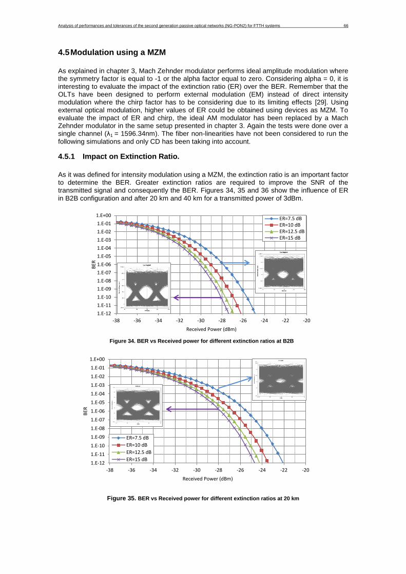
MASTER THESIS TITLE: Analysis of performances and tolerances of the second generation passive optical networks (NG-PON2) for FTTH systems MASTER DEGREE: Master in Science in Telecommunication Engineering & Management AUTHOR: Juan Camilo Velásquez Micolta DIRECTOR: Josep Joan Prat Gomà DATE: September 30th 2014
Transcript
MASTER THESIS
TITLE: Analysis of performances and tolerances of the second generation passive optical networks (NG-PON2) for FTTH systems MASTER DEGREE: Master in Science in Telecommunication Engineering & Management AUTHOR: Juan Camilo Velásquez Micolta DIRECTOR: Josep Joan Prat Gomà DATE: September 30th 2014
Analysis of performances and tolerances of the second generation passive optical networks (NG-PON2) for FTTH systems 2
Título: Análisis de rendimientos y tolerancias de las redes ópticas pasivas de segunda generación (NG-PON2) para sistemas FTTH. Autor: Juan Camilo Velásquez Micolta Director: Josep Joan Prat Gomà Fecha: 30 de Septiembre de 2014
Resumen
En un Sistema de Fibra hasta el hogar (FTTH, Fiber to the Home), la fibra es conectada hasta el hogar de los usuarios. Una red óptica pasiva (PON) es un tipo particular de red redes FTTH que utiliza instalaciones punto a multipunto (P2MP), en las cuales se comparte parte de la infraestructura permitiendo enviar información de múltiples canales a través de una sola fibra. Este trabajo presenta un compendio de los principales conceptos sobre redes de acceso y sistemas PON y algunas de las tecnologías usadas para el desarrollo de los mismos, incluyendo multiplexación por división en el tiempo (TDM, Time Division Multiplexing) y multiplexación por división de la longitud de onda (WDM, Wavelength Division Multiplexing), independientes o en configuración híbrida (TWDM). A partir de aquí se identifican y modelan los dispositivos comerciales clave para su implementación, especificando sus parámetros característicos para cumplir con los requerimientos del nuevo estándar internacional ITU-T G.989 para redes FFTH. Este proyecto evalúa dicho estándar, el cual plantea la implementación de sistemas NG-PON2 a 4x10GBit/s, los cuales usarán una arquitectura híbrida TWDM y transceptores sintonizables, además de garantizar la coexistencia con otros sistemas PON heredados, ubicando el tráfico en downstream y upstream en unas bandas de longitud de onda adecuadas sin solapamiento. El trabajo de análisis se enfoca en la identificación de los dispositivos clave, como trasmisores y filtros ópticos sintonizables para alcanzar los requerimientos mímos especificados. Además se da una primera aproximación al diseño del elemento de coexistencia (CE, Coexistence element) para el soporte de los sistemas PON heredados. Una vez especificados los requerimientos mínimos e identificados los dispositivos clave, se diseña e implementa la red en el simulador VPIphotonicsTM usando láseres de onda continua, moduladores externos de intensidad, multiplexores de longitud de onda y divisores de potencia apropiados. En recepción se usa detección directa con fotodiodos PIN y APD y filtros ópticos sintonizables en la ONU. Una vez completado el diseño, se realizan diferentes test, se analizan los resultados y se optimiza el diseño para dimensionar la red en términos de número de usuarios, alcance, balance de potencias, capacidad de acho de banda, etc.
Analysis of performances and tolerances of the second generation passive optical networks (NG-PON2) for FTTH systems 3
Title: Analysis of performances and tolerances of the second generation passive optical networks (NG-PON2) for FTTH systems Author: Juan Camilo Velásquez Micolta
Director: Josep Joan Prat Gomà
Date: September 19th 2014
Overview
In a Fiber to the Home (FTTH) system, the fiber is connected until the household users. A passive optical network (PON) is a particular type of FTTH networks that uses P2MP (point-to-multipoint fiber premises) in which part of the infrastructure is shared allowing to send information of multiple channels through one fiber. This study presents a summary of the main concepts about access networks and PON systems and some technologies used to its development, including Time Division Multiplexing (TDM) and Wavelength division multiplexing (WDM), independently or in hybrid configuration (TWDM). From here the key commercial devices for its implementation are identified and modelled, specifying its characteristic parameters to fulfill the minimum requirements of the new international standard ITU-T G.989 for FTTH networks. This project evaluates this standard, which proposes the implementation of NG-PON2 systems at 4x10Gbit/s, that will use a hybrid architecture TWDM and tunable transceivers; it also ensures coexistence with other legacy PON systems allocating the downstream and upstream traffic in appropriate wavelength bands without overlapping. The work of analysis is focused in the identification of key devices, like tunable transmitters and tunable filters to achieve the specified requirements. Besides, a first approximation to the coexistence element (CE) is made, for supporting the legacy PON systems. Once the minimum requirements are specified and the key devices identified, the network is designed and built in the commercial simulator VPIphotonicsTM, using CW laser, external intensity modulators, wavelength multiplexers and the appropriate power splitters. In reception a direct detection scheme is implemented using PIN and APD photodiodes and tunable filters at ONU. Once the design is completed different test are run, the results are analyzed and the design is optimized, in order to dimension the network in terms of fiber reach, number of users, power budget, bandwidth capacity, etc.
Analysis of performances and tolerances of the second generation passive optical networks (NG-PON2) for FTTH systems 4
A mis padres Marlene y Jorge Iván.
A mi tía Miriam.
A mis abuelos Oscar y Mariela.
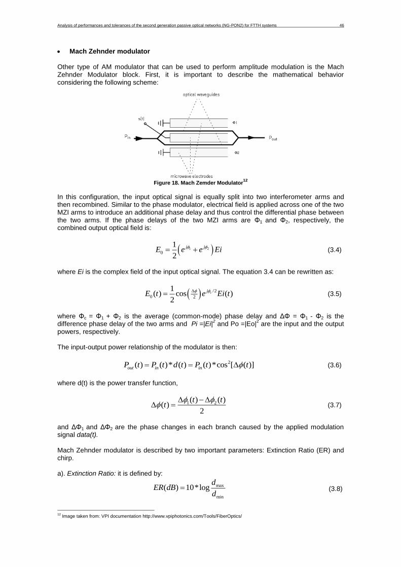
“Y Jesús les habló otra vez, diciendo: Yo soy la luz del mundo; el que me sigue,
no andará en tinieblas, sino que tendrá la luz de la vida”. Jn 8:12
Analysis of performances and tolerances of the second generation passive optical networks (NG-PON2) for FTTH systems 5
Analysis of performances and tolerances of the second generation passive optical networks (NG-PON2) for FTTH systems 6
ACKNOWLEDMENTS
To God for being my spiritual guide in all the tasks of my life. To my family for their constant
support in all the projects I have enrolled.
I would like to thank my advisor Josep Prat for giving me the opportunity to develop a high
relevance project and for the numerous helpful discussions during its development. I am also
indebted to my colleagues at the GCO group for their valuable feedback, encouragement and
advice in the elaboration of this thesis, especially to Victor Polo, Ivan Cano and Adolfo Lerin.
Special thanks to my friend and colleague Jeison Tabares for his support and guide during the
development of this work.
Finally I would like to thank Diana for her support and love during all days that this work was
being developed.
Analysis of performances and tolerances of the second generation passive optical networks (NG-PON2) for FTTH systems 7
ABBREVIATIONS & ACRONYMS ADC – Analogue to digital converters AM – Amplitude Modulation ASE – Amplified Spontaneous Emission APON – ATM Passive Optical Network ATM – Asynchronous Transfer Mode AWG – Arrayed Waveguide Grating BER – Bit Error Rate BPON – Broadband Passive Optical Network C-band – Conventional wavelength band CE – Coexistence element CD – Chromatic dispersion CO – Central Office CW – Continuous Wave DBR – Distributed Bragg Reflector DCM – Dispersion Compensation Module DFB – Distributed Feedback DML – Direct Modulated Laser DSF – Dispersion Shifted Fiber DWDM – Dense Wavelength Division Multiplexing EAM – Electro-Absorption Modulator EML – External Modulated Laser ECL – External Cavity Laser EDFA – Erbium Doped Fiber Amplifier EPON – Ethernet Passive Optical Network ER – Extinction Ratio FP – Fabry-Perot FSAN – Full Service Access Network FSR – Free Spectral Range FTTH – Fiber To The Home FWHM – Full Width at Half Maximum FWM – Four Wave Mixing GbE – Gigabit Ethernet GPON – Gigabit Passive Optical Network
G-EPON – 10 Gbit/s Ethernet Passive Optical Network GVD – Group Velocity Dispersion IEEE – Institute of Electrical and Electronics Engineers IP – Internet Protocol ISI – Inter-Symbol Interference ITU – International Telecommunication Union L-band – Long wavelength band LiNbO3 – Lithium Niobate MEMS – Micro Electro-Mechanical System MPN – Mode Partition Noise MZ – Mach Zehnder MZM – Mach Zehnder Modulator NG-PON2 – Second Generation Passive Optical Network NLSE – Nonlinear Lineal Scrödinger Equation NRZ – Non-Return-to-Zero OADM – Optical Add Drop Multiplexer OEO – Optical-to-Electrical-to-Optical OLT – Optical Line Terminal ONU – Optical Network Unit ONT – Optical Network Terminal OOK – On-Off Keying OSA – Optical Spectrum Analyser OSNR – Optical Signal to Noise Ratio PC – Polarization Controller PIC – Photonic Integrated Circuit
Analysis of performances and tolerances of the second generation passive optical networks (NG-PON2) for FTTH systems 8
PLC – Planar Lightwave Circuits PMD – Physical Media Dependent PON – Passive Optical Network PPG – Pulse Pattern Generator PRBS – Pseudorandom Binary Sequence PtMP – Point to Multipoint PtP – Point to Point QoS – Quality of Service RF – Radio Frequency RMS – Root-Mean-Squared RZ – Return-to-Zero RX – Receiver SE – Spectral Efficiency SMF – Single Mode Fiber SMSR – Side Mode Suppression Ratio SOA – Semiconductor Optical Amplifiers TC – Transmission Convergence TDM – Time Division Multiplexing TEC – Thermo Electric Cooler TL – Tunable Laser TTX – Tunable Transmitter TX – Transmitter TWDM – Time & Wavelength Division Multiplexing UDWDM – Ultra Dense Wavelength Division Multiplexing VCSEL – Vertical Cavity Surface Emitting Lasers VoIP – Voice over Internet Protocol VPI – Virtual Photonics Incorporated WDM – Wavelength Division Multiplexing
XG-PON – 10-Gigabit Passive Optical Network
Analysis of performances and tolerances of the second generation passive optical networks (NG-PON2) for FTTH systems 9
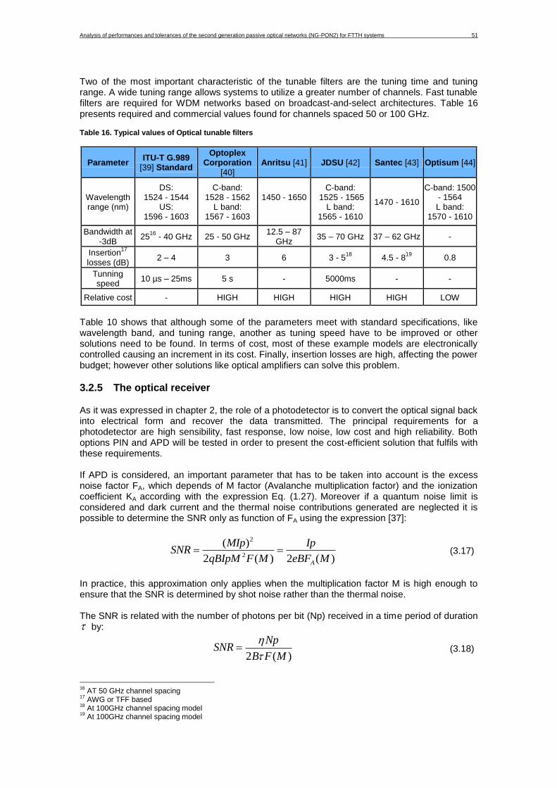
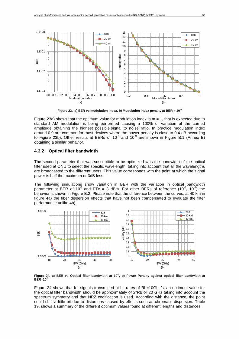
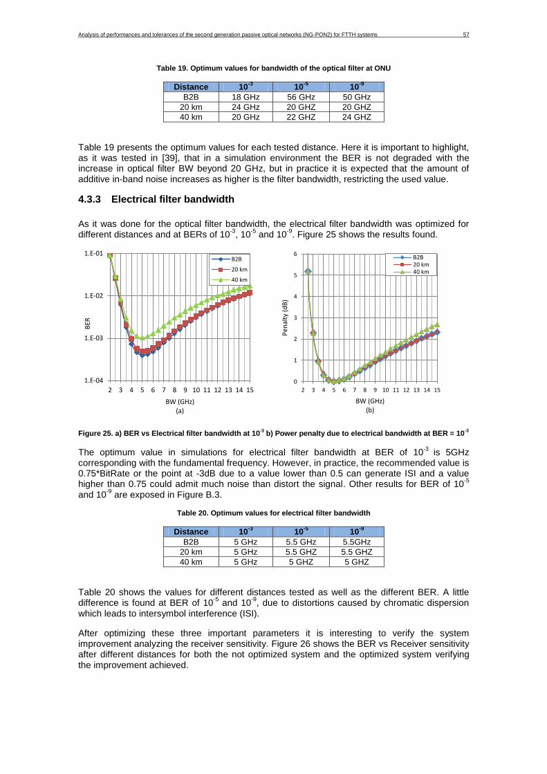
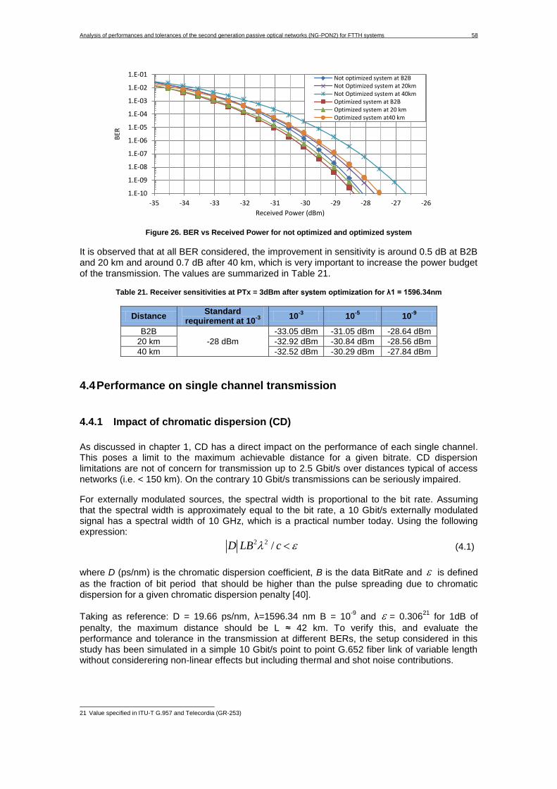
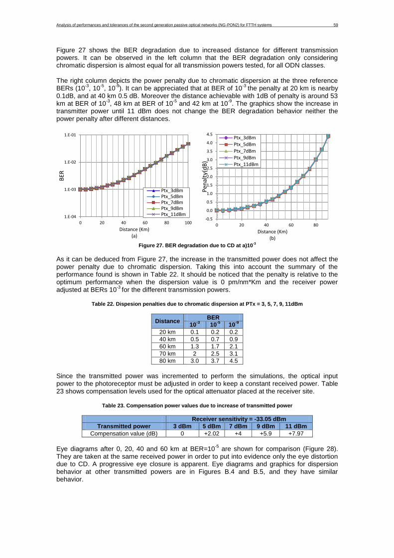
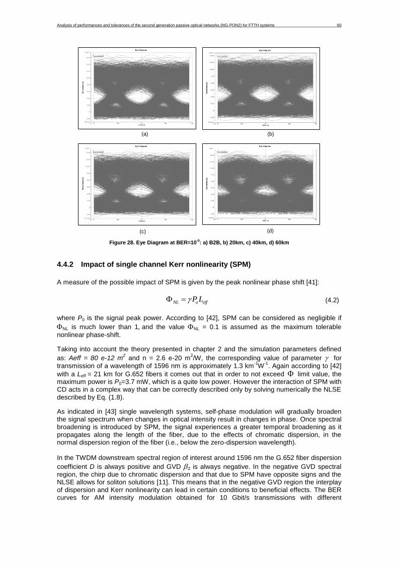
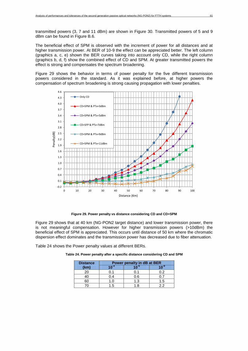
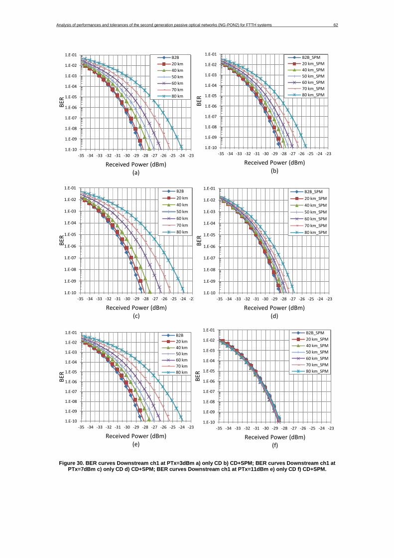
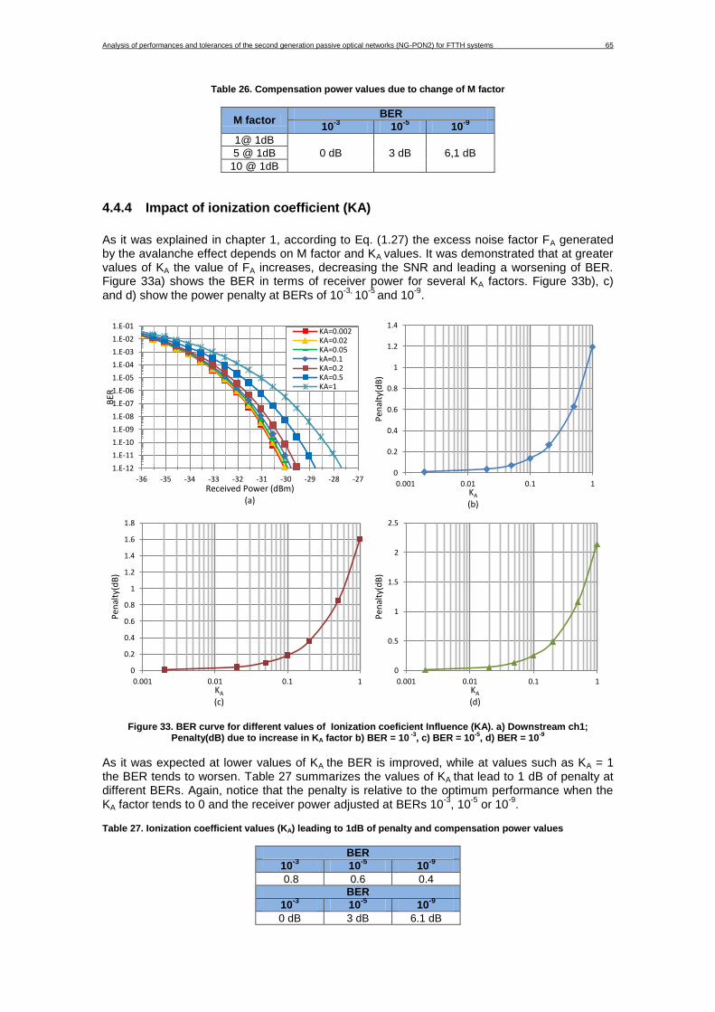
CHAPTER 4. COMPUTER SIMULATION RESULTS, ANALYSIS OF PERFORMANCES AND SYSTEM OPTIMIZATION ........................................................................................................... 54
4.4 Performance on single channel transmission .............................................................. 58 4.4.1 Impact of chromatic dispersion (CD) .................................................................... 58 4.4.2 Impact of single channel Kerr nonlinearity (SPM) ................................................ 60 4.4.3 Impact of shot and thermal noise ......................................................................... 63 4.4.4 Impact of ionization coefficient (KA) ..................................................................... 65
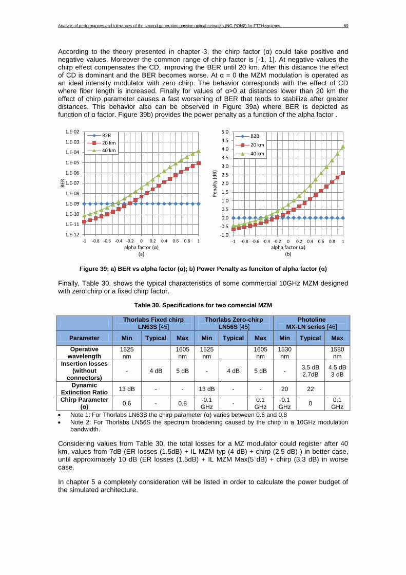
4.5 Modulation using a MZM ................................................................................................. 66 4.5.1 Impact on Extinction Ratio. ................................................................................... 66 4.5.2 Impact on chirp over transmission using MZM ..................................................... 68
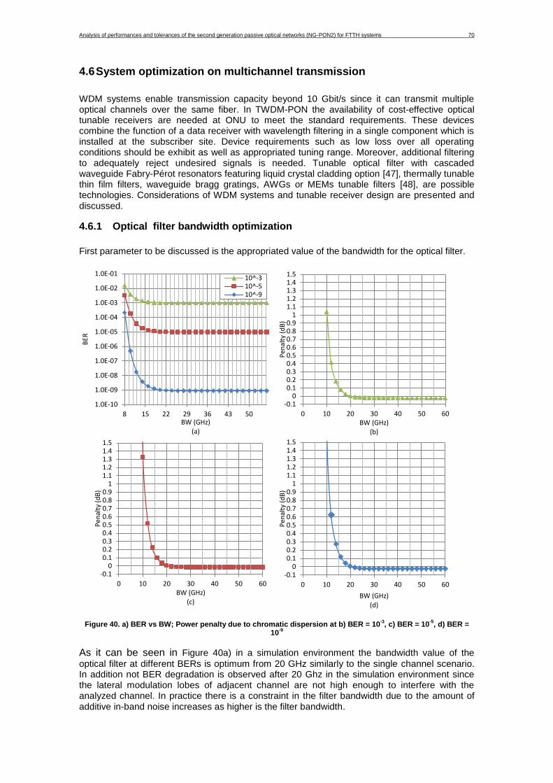
4.6 System optimization on multichannel transmission ................................................... 70 4.6.1 Optical filter bandwidth optimization .................................................................... 70 4.6.2 Channel spacing tolerance ................................................................................... 71 4.6.3 Impact on multichannel Kerr nonlinearity (SPM, XPM) and Impact on multichannel Ramman Scatering ............................................................................................................ 71
4.7 Downstream and Upstream inter-channel crosstalk analysis .................................... 73
CHAPTER 5.TWDM-PON DIMENSIONING FOR NG-PON2 ..................................................... 76
5.1 Power budget analysis and network dimensioning ..................................................... 76
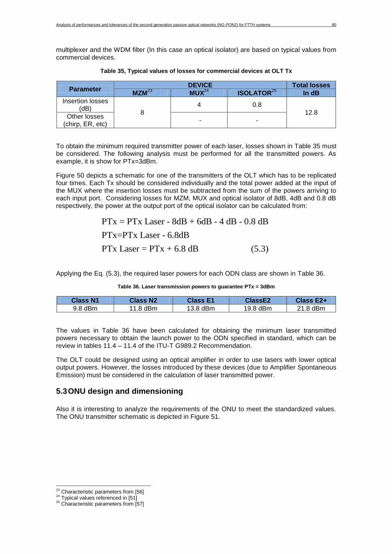
5.2 OLT design and dimensioning ....................................................................................... 79
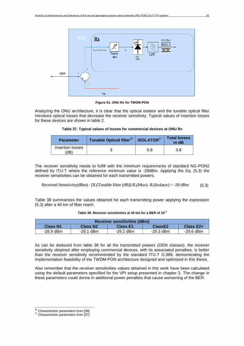
5.3 ONU design and dimensioning ...................................................................................... 80
Analysis of performances and tolerances of the second generation passive optical networks (NG-PON2) for FTTH systems 11
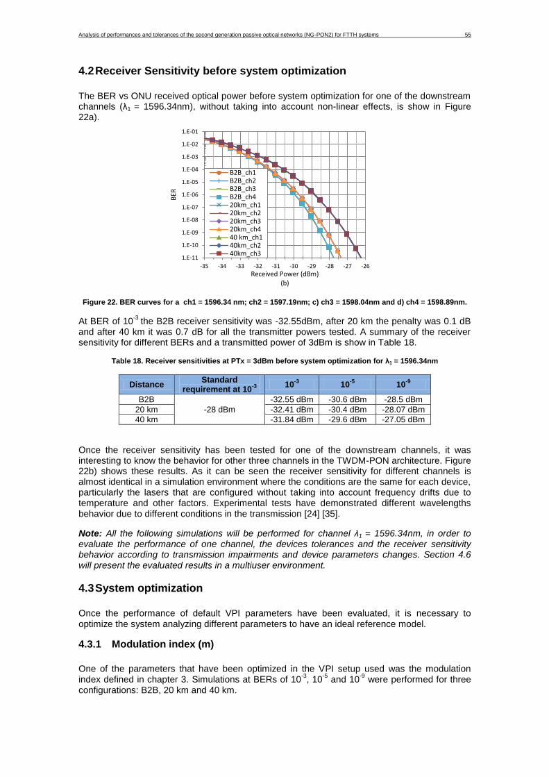
LIST OF FIGURES Figure 1. PON systems and elements ........................................................................................ 16 Figure 2. a)TDM Network Architecture and b)WDM Network Architecture (using an AWG as MUX/DEMUX) ............................................................................................................................. 17 Figure 3. Hybrid WDM/TDM architecture .................................................................................... 18 Figure 4. TWDM PON architecture ............................................................................................. 19 Figure 5. Timeline of the evolution of the PON networks standards ........................................... 20 Figure 6. Next-generation PON (NG-PON) stages and evolution ............................................... 20 Figure 7. Attenuation regions in optical fibers ............................................................................. 21 Figure 8. Direct modulation scheme (left) and external modulation scheme (right) ................... 26 Figure 9. Excess noise factor FA as an function of the average APD gain M for several values of KA ................................................................................................................................................ 29 Figure 10. Differential distance concept ...................................................................................... 32 Figure 11. General architecture for NG-PON2 system coexistence with legacy PONs .............. 33 Figure 12. Detailed architecture of a TWDM-PON ...................................................................... 34 Figure 13. OLT Transceiver for NG-PON2 .................................................................................. 35 Figure 14. ONU Transceiver for NG-PON2 ................................................................................. 35 Figure 15. Wavelength plans and availability of PON systems ................................................... 36 Figure 16. a) OLT architecture; b) ONU architecture .................................................................. 41 Figure 17. General system architecture used in the simulations ................................................ 42 Figure 18. Mach Zemder Modulator ............................................................................................ 46 Figure 19. Theoretical model for APD photoreceiver for different values of M ........................... 52 Figure 20. Ber vs Reciever power for different values of M factor .............................................. 53 Figure 21. BER vs Received power for a) PIN photodiode, b) APD photodiode. ....................... 54 Figure 22. BER curves for a ch1 = 1596.34 nm; ch2 = 1597.19nm; c) ch3 = 1598.04nm and d) ch4 = 1598.89nm. ........................................................................................................................ 55 Figure 23. a) BER vs modulation index, b) Modulation index penalty at BER = 10
-3 ................. 56
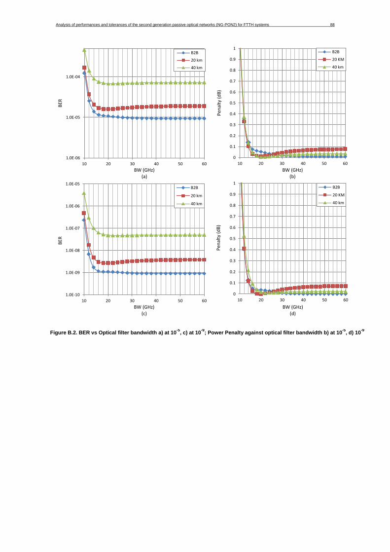
Figure 24. a) BER vs Optical filter bandwidth at 10-3
, b) Power Penalty against optical filter bandwidth at BER=10
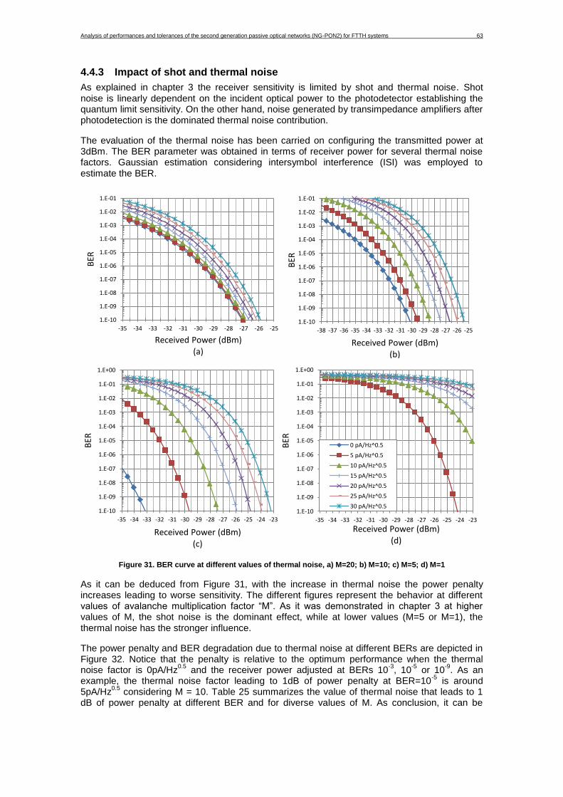
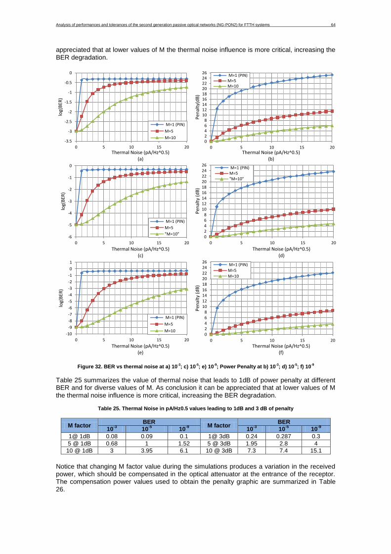
: a) B2B, b) 20km, c) 40km, d) 60km................................ 60 Figure 29. Power penalty vs distance considering CD and CD+SPM ........................................ 61 Figure 30. BER curves Downstream ch1 at PTx=3dBm a) only CD b) CD+SPM; BER curves Downstream ch1 at PTx=7dBm c) only CD d) CD+SPM; BER curves Downstream ch1 at PTx=11dBm e) only CD f) CD+SPM. .......................................................................................... 62 Figure 31. BER curve at different values of thermal noise, a) M=20; b) M=10; c) M=5; d) M=1 63 Figure 32. BER vs thermal noise at a) 10
-3; c) 10
-5; e) 10
-9; Power Penalty at b) 10
-3; d) 10
-5; f)
10-9
............................................................................................................................................... 64 Figure 33. BER curve for different values of Ionization coeficient Influence (KA). a) Downstream ch1; Penalty(dB) due to increase in KA factor b) BER = 10
-3, c) BER = 10
-5, d) BER = 10
-9 ..... 65
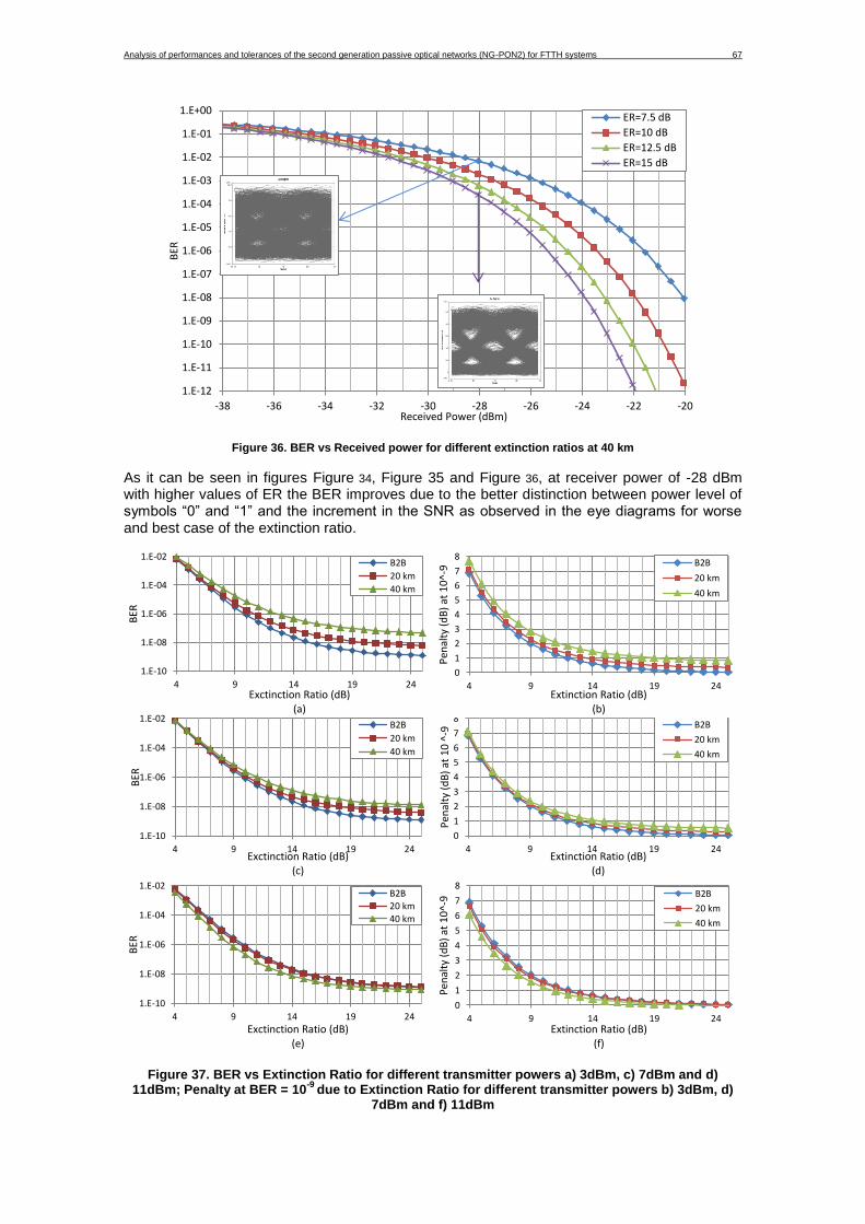
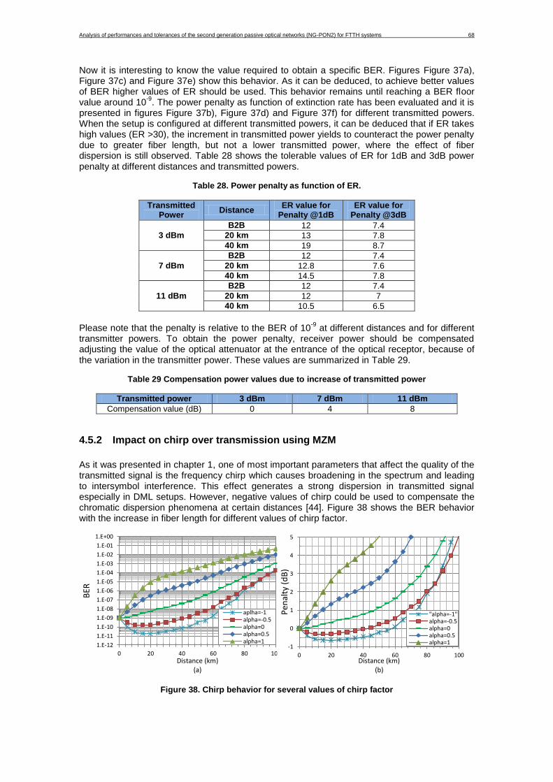
Figure 34. BER vs Received power for different extinction ratios at B2B ................................... 66 Figure 35. BER vs Received power for different extinction ratios at 20 km ................................ 66 Figure 36. BER vs Received power for different extinction ratios at 40 km ................................ 67 Figure 37. BER vs Extinction Ratio for different transmitter powers a) 3dBm, c) 7dBm and d) 11dBm; Penalty at BER = 10
-9 due to Extinction Ratio for different transmitter powers b) 3dBm,
d) 7dBm and f) 11dBm ................................................................................................................ 67 Figure 38. Chirp behavior for several values of chirp factor ....................................................... 68 Figure 39; a) BER vs alpha factor (α); b) Power Penalty as funciton of alpha factor (α) ............ 69 Figure 40. a) BER vs BW; Power penalty due to chromatic dispersion at b) BER = 10
-3, c) BER
= 10-5
, d) BER = 10-9
.................................................................................................................... 70 Figure 41. a) BER against channel spacing (df); b) Power penalty at BER = 10
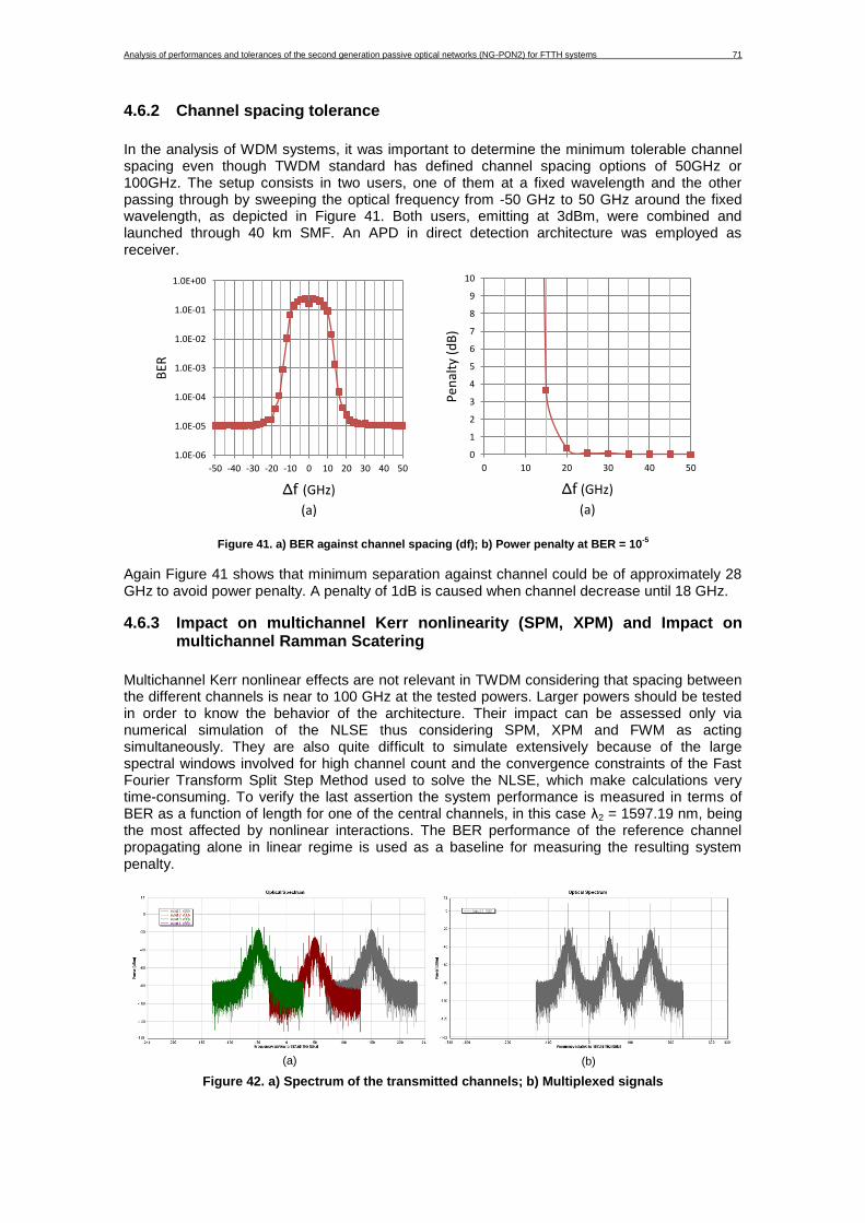
-5 ..................... 71
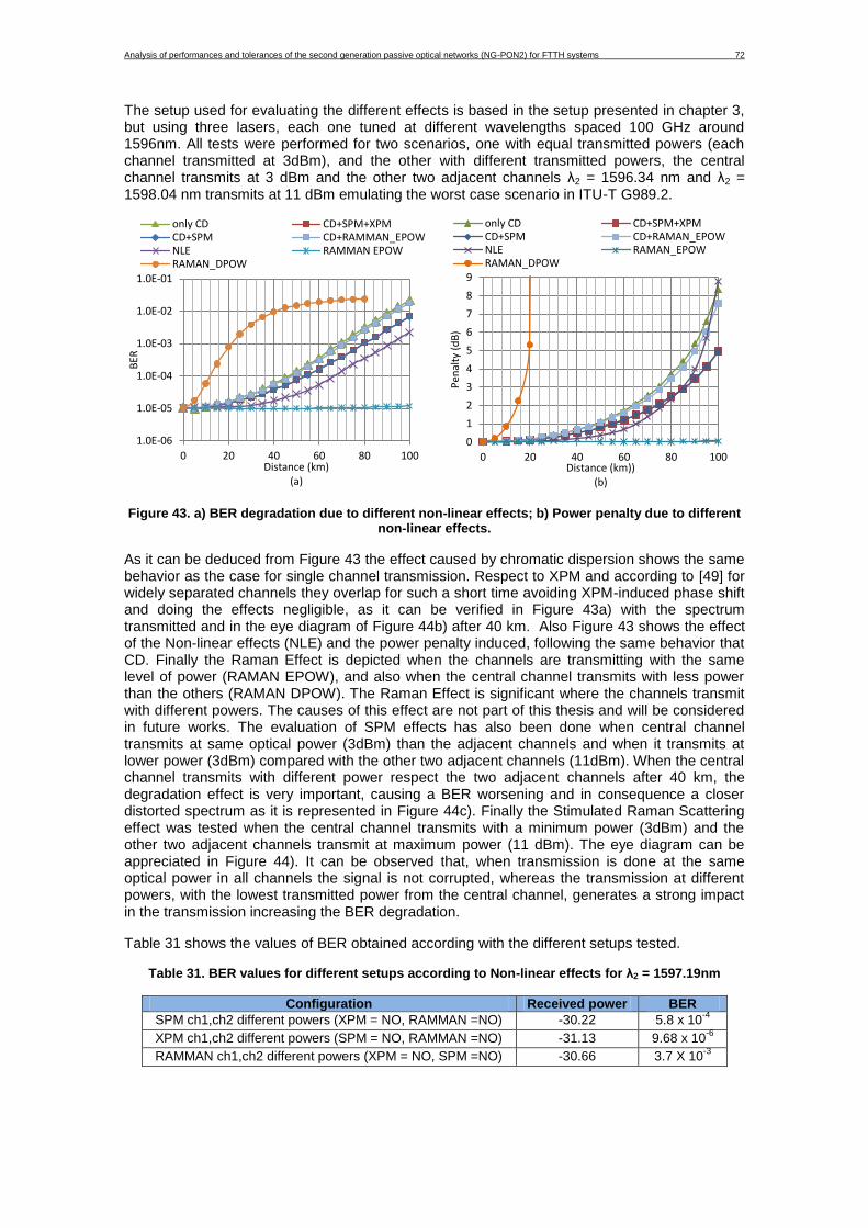
Figure 42. a) Spectrum of the transmitted channels; b) Multiplexed signals .............................. 71 Figure 43. a) BER degradation due to different non-linear effects; b) Power penalty due to different non-linear effects. .......................................................................................................... 72
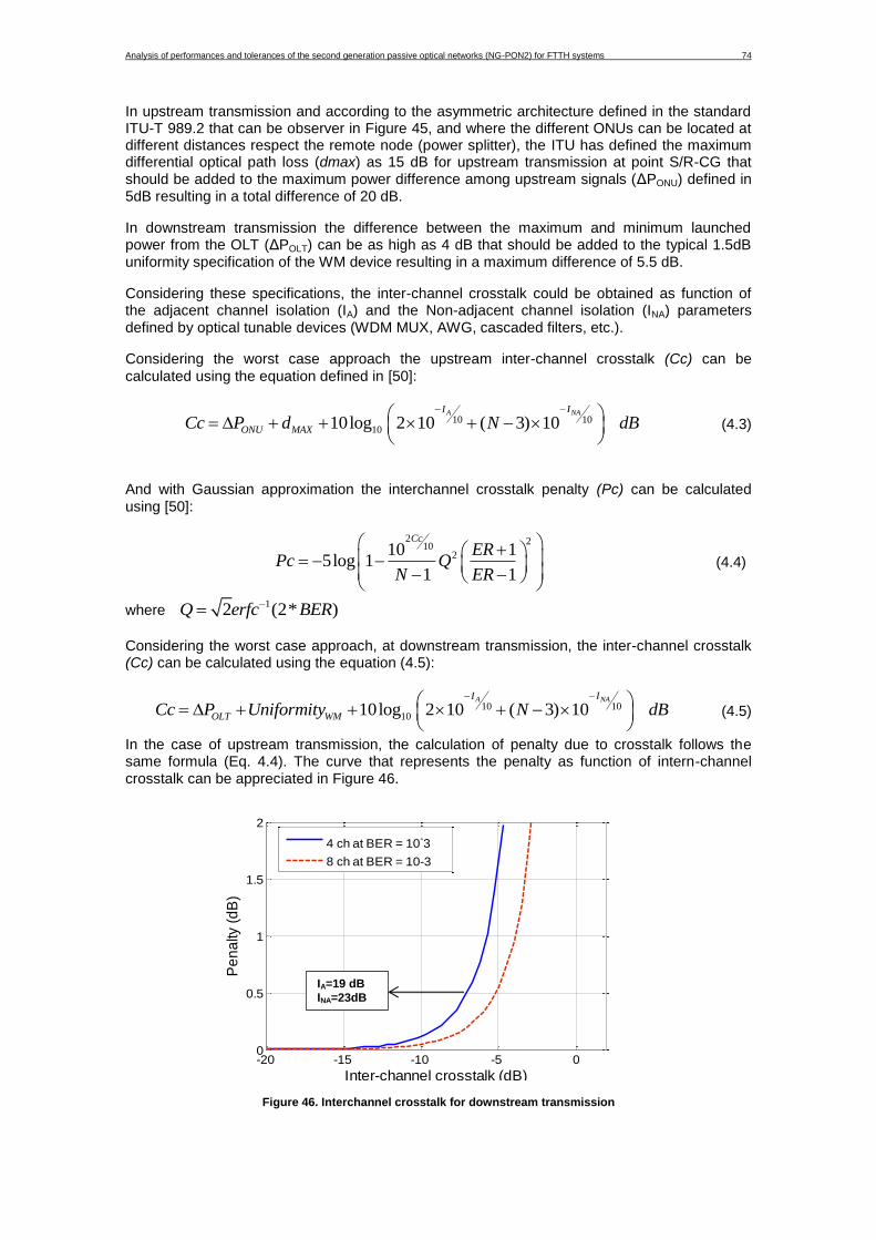
Analysis of performances and tolerances of the second generation passive optical networks (NG-PON2) for FTTH systems 12
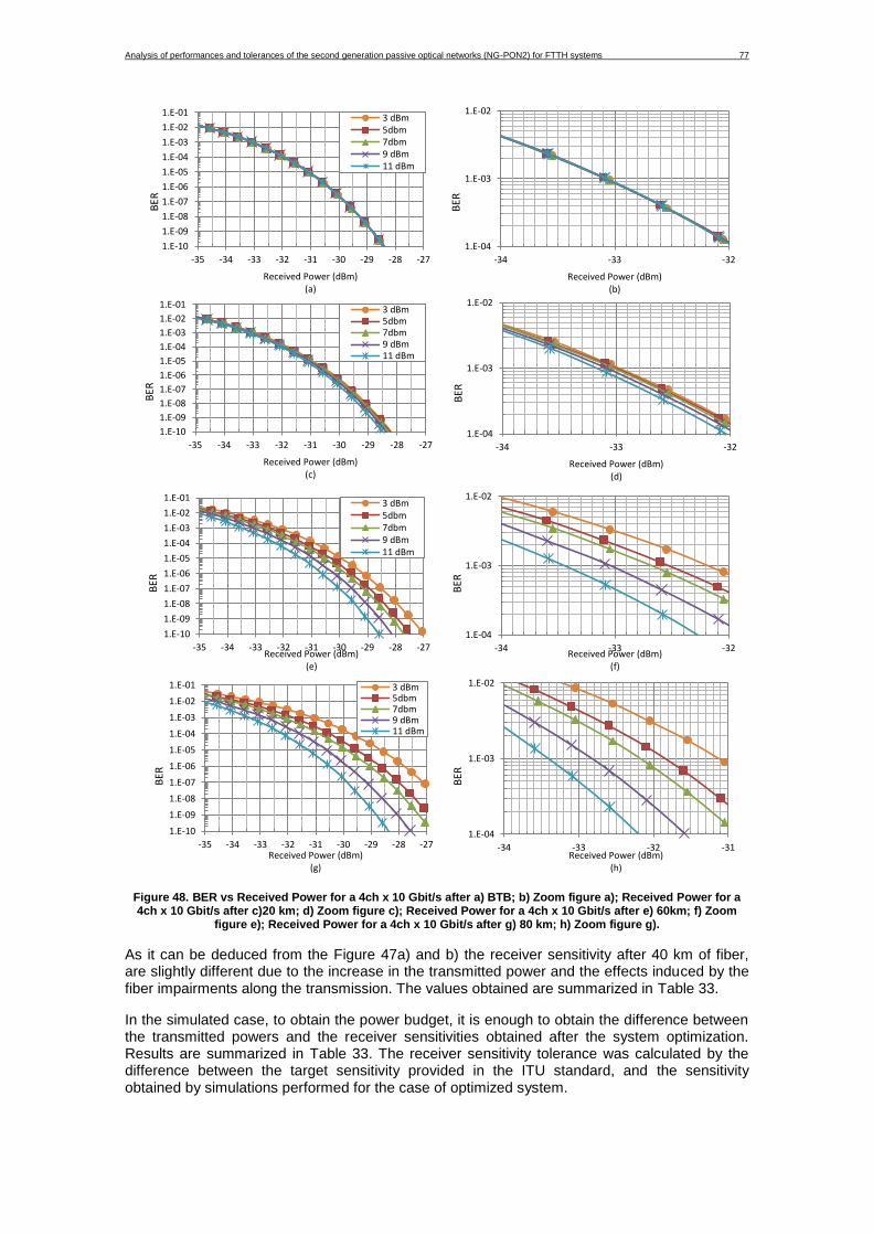
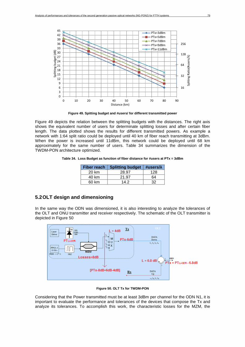
Figure 44. a) Spectrum of received signal after 40 km considering XPM; b) Eye diagram after 40km considering XPM; c) Eye diagram of the received signal after 40 km considering SPM and adjacent channels with different transmitted powers; d) Eye diagram of the received signal after 40 km considering Raman effect and adjacent channels with different transmitted powers ...... 73 Figure 45. Reference diagram for inter-channel crosstalk calculation ........................................ 73 Figure 46. Interchannel crosstalk for downstream transmission ................................................. 74 Figure 47. a) BER vs Received Power for a 4ch x 10 Gbit/s after a) 40 km; b) Zoom figure 1a) 76 Figure 48. BER vs Received Power for a 4ch x 10 Gbit/s after a) BTB; b) Zoom figure a); Received Power for a 4ch x 10 Gbit/s after c)20 km; d) Zoom figure c); Received Power for a 4ch x 10 Gbit/s after e) 60km; f) Zoom figure e); Received Power for a 4ch x 10 Gbit/s after g) 80 km; h) Zoom figure g). ............................................................................................................ 77 Figure 49. Spitting budget and #users/ for different transmitted power ...................................... 79 Figure 50. OLT Tx for TWDM-PON ............................................................................................. 79 Figure 51. ONU Rx for TWDM-PON ........................................................................................... 81
Analysis of performances and tolerances of the second generation passive optical networks (NG-PON2) for FTTH systems 13
LIST OF TABLES Table 1. Characteristics of TWDM PON ..................................................................................... 19 Table 2. NG-PON2 splitting ratio options .................................................................................... 32 Table 3. Wavelength bands defined by IT for NG-PON2 based in TWDM ................................. 36 Table 4. TWDM-PON Downstream and Upstream Channel Grid Examples .............................. 36 Table 5. Typical interface parameters ONU and OLT for TWDM [19] ........................................ 38 Table 6. Characteristic parameters of two experimental setups of TWDM-PON ........................ 39 Table 7. Device and component VPI parameters ....................................................................... 44 Table 8. Important parameters for WM ....................................................................................... 47 Table 9. Attenuation fiber coefficient (α’) in deployment environment [30] ................................. 48 Table 10. Reflectance and insertion losses due to splices, & connectors [31] ........................... 48 Table 11. Reference values ........................................................................................................ 49 Table 12. Reference values for dispersion coefficient and dispersion slope [30] ....................... 49 Table 13. Typical values for Uniformity paramter for Power splitters [31]................................... 50 Table 14. PDL values for power splitter [31] ............................................................................... 50 Table 15. Insertion losses for power splitter [31] ......................................................................... 50 Table 16. Typical values of Optical tunable filters ....................................................................... 51 Table 17. APD default simulation parameters ............................................................................. 54 Table 18. Receiver sensitivities at PTx = 3dBm before system optimization for λ1 = 1596.34nm ..................................................................................................................................................... 55 Table 19. Optimum values for bandwidth of the optical filter at ONU ......................................... 57 Table 20. Optimum values for electrical filter bandwidth ............................................................ 57 Table 21. Receiver sensitivities at PTx = 3dBm after system optimization for λ1 = 1596.34nm 58 Table 22. Dispesion penalties due to chromatic dispersion at PTx = 3, 5, 7, 9, 11dBm ............. 59 Table 23. Compensation power values due to increase of transmitted power ........................... 59 Table 24. Power penalty after a specific distance considering CD and SPM ............................. 61 Table 25. Thermal Noise in pA/Hz0.5 values leading to 1dB and 3 dB of penalty ..................... 64 Table 26. Compensation power values due to change of M factor ............................................. 65 Table 27. Ionization coefficient values (KA) leading to 1dB of penalty and compensation power values .......................................................................................................................................... 65 Table 28. Power penalty as function of ER. ................................................................................ 68 Table 29 Compensation power values due to increase of transmitted power ............................ 68 Table 30. Specifications for two comercial MZM ......................................................................... 69 Table 31. BER values for different setups according to Non-linear effects for λ2 = 1597.19nm . 72 Table 32. Values of Interchannel crosstalk and power penalty for commercial WM in worse case approach for upstream transmission ........................................................................................... 75 Table 33. Receiver sensitivities and Link Budget for different ODN classes in a 4 ch x 10 Gbit/s TWDM-PON architecture at BER of 10-3 .................................................................................... 78 Table 34. Loss Budget as function of fiber distance for #users at PTx = 3dBm ........................ 79 Table 35, Typical values of losses for commercial devices at OLT Tx ....................................... 80 Table 36. Laser transmission powers to guarantee PTx = 3dBm ............................................... 80 Table 37. Typical values of losses for commercial devices at ONU Rx ...................................... 81 Table 38. Receiver sensitivities at 40 km for a BER of 10
Analysis of performances and tolerances of the second generation passive optical networks (NG-PON2) for FTTH systems 14
INTRODUCTION
The continued growth in services such as VoIP, live video streaming and peer to peer communications has led to a corresponding increase in consumer bandwidth demand for high-speed fiber connections, both to the home and to the business.
Passive optical networks (PONs) are being installed through several countries to provide broadband services. The evolution of PON systems across the years can be associated with the evolution in multiplexing technologies. In the first years with the use of ATM-based PON (APON and BPON), the achieved upstream and downstream aggregate bandwidths were in the order of 155 Mbit/s up to 622 Mbit/s. Later, the use of time division multiplexing (TDM) permitted achieving capacities around 1.2 Gbit/s and 2.5 Gbit/s (downstream & upstream) according with the ITU-T G.984 G-PON standard. Advanced high-speed TDM based optical access systems up to 10Gbit/s for downstream and 2.5 upstream (XG-PON1) or 10Gbit/s/ for both downstream and upstream (XG-PON2), according with the ITU-T G.987 G-PON standard, have been developed and some field trials have been reported. Currently, standardized specifications by ITU exist for ATM-based PON (APON and BPON), gigabit-capable PON (GPON) and XG-PON and Ethernet PON (EPON) and 10G-EPON by IEEE.
However, with the implementation of Wavelength Division Multiplexing (WDM) in transport networks, the capacities have been increased significantly until achieving bandwidths of 250 GBit/s and 500 GBit/s using ud-WDM with coherent detection in the research field. The standardization of the next generation optical access networks operating at over 10-Gbit/s has started to consider more flexible network configuration using WDM and to respond to those demands. Time and Wavelength Division Multiplexing (TWDM-PON) emerge as one of the most promising PON solutions in which each wavelength is shared between multiple Optical Networks Units (ONUs) by employing TDMA mechanism to provide high capacity to supply the bandwidth demand of broadband services.
For several years FSAN and IEEE have been working on the new international standard ITU-T G.989: 40-Gigabit-capable passive optical networks (NG-PON2) which general requirements have been defined on ITU-T G989.1 standard by March of 2013. However the PMD (ITU-T G989.2) and TC layer requirements (ITU-T G989.3) are still being discussed and are expected to be published soon.
The lightwave technology, based on the use of light in place of microwaves, has advanced in different fields including lasers, optical fibers and other optical devices and subsystems. A multitude of silica and semiconductor-based components and optical devices have emerged to fit the new WDM scenarios.
With this work several setups are analyzed considering the architecture shown in the standard and the availability of the optical devices, focusing in the tunable transceivers and tunable filters at ONU.
Taking this scenario as starting point, this thesis will evaluate the new international standard for the FTTH networks implementing NG-PON2 systems operating at 4x10GBit/s, especially the PMD requirements, in order to determine the key commercial devices for its implementation. The devices will be modeled and the access network will be built in a computer simulator, different tests will be run, and the system will be optimized.
A large number of papers, especially from international congresses ECOC2013 and OFC2014, have been checked with the different proposals from different vendors and research groups. Moreover the physical requirements of the standard have been evaluated and the tolerances and performances of different commercial devices are compared.
At the end a cost-efficient architecture is proposed based in the technology available taking into consideration the different results and optimizations made.
Analysis of performances and tolerances of the second generation passive optical networks (NG-PON2) for FTTH systems 15
OBJECTIVES AND THESIS OUTLINE
Objectives
In this thesis the main objective is doing a deep study of a proposed hybrid time and wavelength division multiplexing passive optical network (TWDM-PON) architecture, analyzing the performance and tolerances of reach of the optical network and the devices in presence of linear and nonlinear impairments.
The specific objectives are:
1. To review the state of art of optical access networks, comparing different technologies, devices and architectures, studying different publications from optical lightwave journals, international conferences (ECOC, OFC, etc.) and the different ITU and IEEE standard for passive optical networks.
2. To analyze the new international standard ITU-T G-989 covering different topics like the wavelength plan, device parameters, system and subsystems minimum requirements and the TWDM-PON PDM layer requirements.
3. To design a NG-PON2 architecture model based in the standard design using cost-efficient devices in order to get the better and reliable performances. These devices and other subsystems (ODN, OLT, ONU) will be modeled and math analyzed and their tolerances defined taking into consideration the commercial devices available from different vendors.
4. To compare the reference values with the ones generated in the computer simulations with the commercial software VPItransmission Maker®, based on the design proposed and some numerical references found in the specialized bibliography.
5. To optimize the NG-PON2 proposed design in order to achieve better transmission quality
values limited by the devices tolerances and linear and non-linear impairments trying to improve the results with respect to the standard ITU-T G.989 minimum.
Thesis Outline
This thesis is structured into five chapters as follows:
Chapter 1 introduces the state of art of FTTH systems and PON. Main concepts and elements are explained, different technologies such as TDM, WDM or the hybrid TWDM are presented and the evolution of the legacy PON systems is shown. Also some basic concepts about the transmission impairments are presented as well as basic concepts about key optical devices.
Chapter 2 discusses the standard G.989 in depth, analyzing different aspects such as the spectrum management, NG-PON2 architecture, PMD layer parameters (split ratio, fiber reach, extinction ratio, etc.), system requirements (Colorless ONU, spectral flexibility, reach extender modules, interoperability). Finally other specific values based on the two line rate options for upstream and downstream are detailed in different tables and schemes. Also some TWDM-PON tests are presented in order to encompass some proposals for real implementations of the new standard.
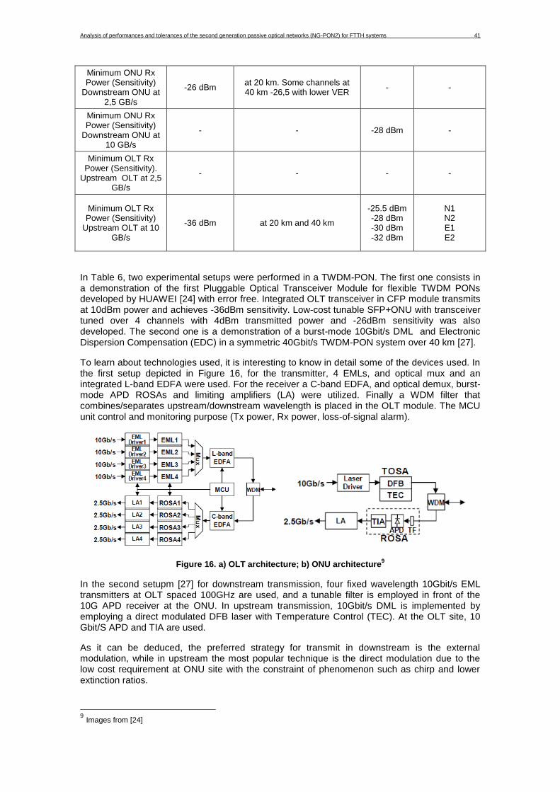
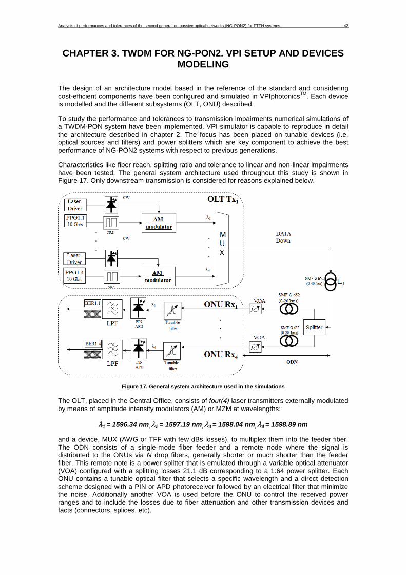
Chapter 3 focuses on the design of an architecture model based in the reference of the standard and considering cost-efficient components. Each device is modeled and the different subsystems (OLT, ONU) described.
Chapter 4 presents the computer simulation results of the design proposed, with different setups, tests and comparisons to analyze and determine the better options. The different transmission impairments are discussed and the final design is optimized. An study of interchannel crosstalk in WDM systems is done based on the ITU-T G.989 Recommendation.
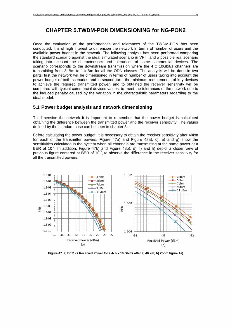
Chapter 5 provides the network dimensioning in terms of numbers of users and distance, as well as the tolerances of devices used in the ONU and OLT design.
Analysis of performances and tolerances of the second generation passive optical networks (NG-PON2) for FTTH systems 16
CHAPTER 1. STATE-OF-THE-ART
1.1 Active vs. Passive Optical Networks
The general structure of a telecommunication network consists of three main portions: Backbone (or Core) Network, metro/regional network, and access network. Backbone networks are used for long-distance transport and metro/regional networks for grooming and multiplexing functions, managing higher aggregated traffic.
An optical access network, also called Fiber to the “x” (FTTx) networks (where “x” can be “home”, “curb”, “premises”, etc., depending on how deep in the field fiber is deployed or how close is to the user) connects the final users to their immediate service provider, feeding the core networks. In a Fiber to the Home (FTTH) system, the fiber is connected until the household users [1]. Compared with metro and backbone networks, access networks manage links with lower speed rates and bandwidth capacities. Access networks can be PtP (Point-to-point) or P2MP (Point-to-multi point).
A passive optical network (PON) is a particular type of FTTx networks that uses P2MP fiber premises, in which unpowered remote nodes are used to share part of the infrastructure, enabling a single optical fiber to serve multiple premises. Compared with an Active Optical Network (AON), where electrically powered switching equipment is used, a PON network uses optical splitters to separate and collect signal reducing the amount of fiber and the Central Office (CO) equipment required, with many economic advantages from installation and maintenance of active devices.
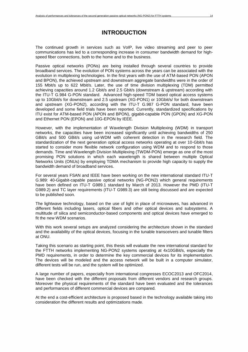
1.2 Elements of a PON
A PON consists on an OLT (Optical Line Terminal) at the service provider's site, a number of ONU (Optical Network Unit) near to end users and passive components called Nodes (RN). The distribution of these elements is shown in Figure 1.
Figure 1. PON systems and elements
The OLT resides in the CO and is the equipment that performs conversion between the electrical signals used by the service provider's equipment and the fiber optic signals used by the passive optical network. Also the OLT coordinates the multiplexing income signals from the ONU’s allocating upstream bandwidth to the ONUs.
The ONU resides at or near the customer premise. An ONU is a device that transforms incoming optical signals into electronics at a customer's premises in order to provide telecommunication services over an optical fiber network. An ONU presents a converged interface that permits to introduce services, such as DSL, coaxial cable or Ethernet.
A passive RN corresponds to a passive optical device, which could be a power splitter that divides the optical power from one fiber between several fibers and reciprocally, to combine optical signals from multiple fibers into one, or an optical multiplexor where the incoming information from any input port is filtered and routed to the selected output ports.
Analysis of performances and tolerances of the second generation passive optical networks (NG-PON2) for FTTH systems 17
1.3 PON Architectures
Different kinds of architectures have been analyzed to meet the Second Generation of Passive Optical Networks (NG-PON2) scenario requirements. The main concepts about each one will be presented next.
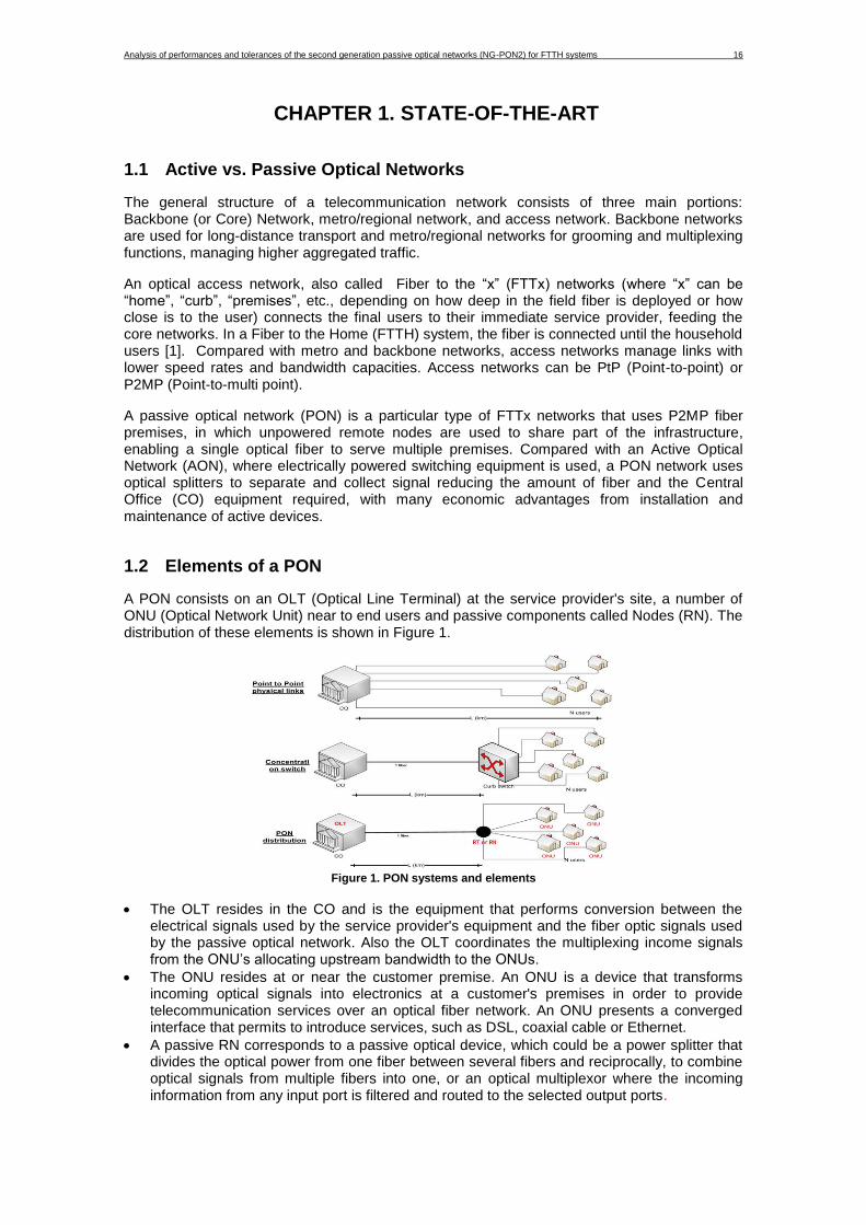
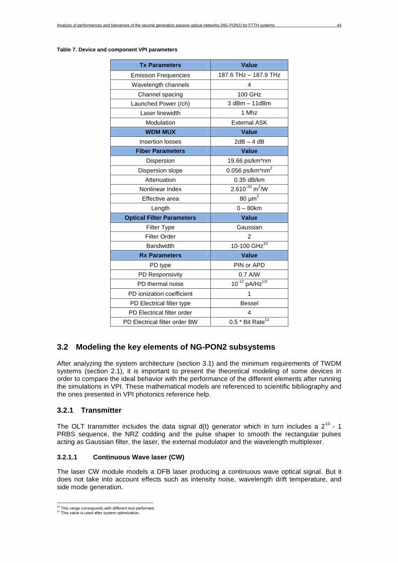
1.3.1 Time Division Multiplexing PON (TDM-PON)
A TDM-PON uses a passive power splitter as the remote node that divide the incoming signal power to the different ONU’s connected. Here, all the users share the same wavelength to transmit the information.
In downstream, the signal from the OLT is multiplexed in different time slots and broadcasted to several ONU’s (weak security), where each ONU recognizes the data through the address labels embedded in the signal. The upstream traffic is transmitted by each ONU in burst mode and a mechanism to avoid collisions must be implemented. Two approaches could be used to provide bidirectional transmission: one or two fibers and one or two wavelengths. So the maximum number of ONUs for TDM is a function of the ONU and ODN implementation with the associated impairments.
Typically in a standard commercial TDM-PON structure the OLT is connected to the ONUs via a 1:32 splitter and the maximum distance covered is usually 20 km. However, in the scientific literature much higher split values up to 1:4000 have been reported [2]. Some advantages of TDM compared with WDM are that it does not require a complex wavelength management control and that the OLT power requirements are lower. However, the main drawbacks are the lower bandwidth and granularity performances. PON standards such as APON, BPON, EPON, G-PON and XG-PON, that have been recently widely deployed, use this architecture, which is shown in Figure 2a).
Figure 2. a)TDM Network Architecture1 and b)WDM Network Architecture (using an AWG as MUX/DEMUX)
A WDM-PON uses a passive WDM coupler as the RN or tunable ONU [2], as shown in Figure 2b). Signals for different ONUs are carried on independent wavelengths and multiplexed on a shared fiber infrastructure. Each ONU could only receive its own wavelength using a tunable filter followed by a photoreceptor to select a specific wavelength or using an optical mux/demux (AWG, thin- film, etc.), creating a logical point-to point connection where each ONU can transmit at its own bit rate without losses by power splitting and dedicated bandwidth with QoS.
WDM has better security than TDM permitting simple fault localization. Also WDM presents better scalability resulting in higher bandwidth capacities, without modification of the TDM infrastructure, and long reaches are achieved. WDM-PON increases the spectral efficiency of the access networks by taking advantage of the high optical bandwidth of optical fibers.
1 Modified from [54]
(a) (b)
Analysis of performances and tolerances of the second generation passive optical networks (NG-PON2) for FTTH systems 18
However WDM devices are significantly more expensive and they are limited by the number of wavelength available, hence powerful OLT are needed. Also each ONU needs a laser tuned in the specific wavelength to transmit or a reflective colorless ONU, so the implementation presents a high cost. Next Generation Fiber to the Home technologies aim to use WDM-PON like the most broadband solution in order to fulfill with the future bandwidth demands.
1.3.3 Hybrid Architectures
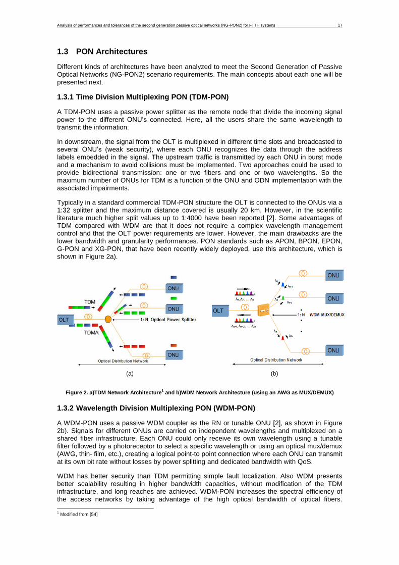
To overcome the problems of WDM PONs, different solutions have been developed in the field of hybrid WDM/TDM in the last years. The idea is to mix both concepts to combine the better of the two options accepting more users and increasing the spectrum efficiency.
Different proposals such as using 100 ns-λ selective-burst mode transceivers for 40 km reach symmetric 40 Gbit/s WDM/TDM-PON [2] or C-band Burst-mode Transmission for High Power Budget (64-split with 40km distance) [3], are examples of these hybrid architectures. Moreover, in order to reduce the stock and to use similar ONUs, colorless technologies have been proposed using different approaches. ONU with tunable distributed feedback lasers (DFB) and temperature control lasers [4], spectrum sliced broadband light sources & injection locked FP lasers [5] or reflective semiconductor optical amplifier [6] are different options.
This is one of the possible architectures that permit to implement both TDM and WDM. First of all a set of wavelengths is thereby fed together via a common, and in general, long trunk or ring segment [8], and a WDM demultiplexer (could be implemented using an AWG like it is shown in Figure 3) spreads the data channels towards a bunch of TDM trees, each of them containing a feeder fiber, a power splitter and a short drop fiber to share the same wavelength among multiple ONUs. In this way a high number of users can be served and it requires low-cost fixed wavelength transceivers at the ONU being this colored. This architecture improves the power budget but reduces the overall flexibility of the PON network.
Figure 3. Hybrid WDM/TDM architecture
1.3.3.2 Time and Wavelength Division Multiplexing PON (TWDM-PON)
The other type of hybrid PONs that is relevant to analyze is called TWDM, where all set of wavelengths that travels through the WDM feeder fiber are broadcasted to all the users using a power splitter as RN and leaving the schedule of the time slots to the MAC layer. In this case the ONU should be colorless (wavelength agnostic) and tunable. This could be achieved by using a RX optical filter tuned at a specific wavelength, and thermally tuned lasers are implemented to transmit in the upstream.
Analysis of performances and tolerances of the second generation passive optical networks (NG-PON2) for FTTH systems 19
Figure 4. TWDM PON architecture
Figure 4 illustrates the TWDM architecture that is the option selected by the FSAN (Full Service Access Networks) for the NG-PON2. This option will be explained in detail along this thesis and will be the scenario to analyze the performance and tolerances of the network subsystems and devices. The principal issues will be the tunable requirements of lasers and filters at the ONU. Table 1 shows the principal characteristics of TWDM-PON architecture.
Table 1. Characteristics of TWDM PON
Parameter TWDM-PON
Aggregate BW 40 GBit/s
User Data 1 GBit/s
Bit Rate per channel 10 Gbit/s
Number of users 256
Wavelength channels 4-8
Wavelength spacing 50-100 GHz
Passive distance reach without reach extender
40 km
Added features Compatibility with legacy PONs
Issues Tunable Laser and filters at ONU
Passive Remote Node Optical Power Splitter
First of all the aggregated bandwidth is higher in WDM/TDM PON scheme as consequence of the higher number of channels. Moreover the reach of the WDM/TDM is higher instead the TWDM aims to guarantee the compatibility with other legacy PONs. Other difference between both architectures is in the ODN, because while in TWDM the RN is a power splitter that broadcasts all the wavelengths to the ONUs and a tunable filter selects the specific wavelength, in WDM/TDM the wavelengths are filtered in the ODN and each of them is routed to a specific TDM tree. This is an advantage of TWDM because the ODN doesn’t require a complex configuration and maintenance using, e.g., a power splitter instead of an AWG so it is backwards compatible with current GPON. Moreover the colorless ONU reduces the need of stock and consequently the network costs.
1.4 Future evolution of PON Systems
The evolution of PON systems across the years can be associated with the evolution in multiplexing technologies. In the first years, with the use of TDM, the achieved upstream and downstream aggregate bandwidth was in the order of 155 Mbit/s until 10 Gbit/s in XG-PON standard taking advantage of FEC. But with the implementation of WDM the capacities have been increased significantly until obtaining bandwidths of 500 Gbit/s using ud-WDM with coherent detection. This new systems use advanced modulation, codification and multiplexing
Analysis of performances and tolerances of the second generation passive optical networks (NG-PON2) for FTTH systems 20
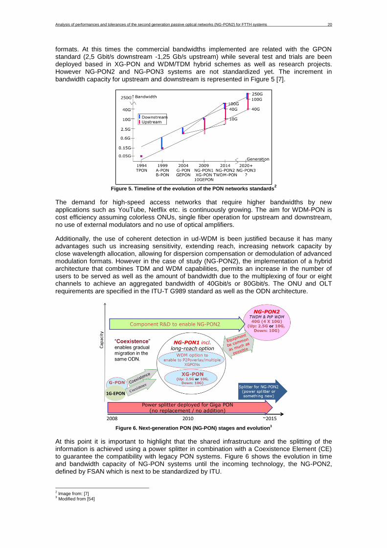
formats. At this times the commercial bandwidths implemented are related with the GPON standard (2,5 Gbit/s downstream -1,25 Gb/s upstream) while several test and trials are been deployed based in XG-PON and WDM/TDM hybrid schemes as well as research projects. However NG-PON2 and NG-PON3 systems are not standardized yet. The increment in bandwidth capacity for upstream and downstream is represented in Figure 5 [7].
Figure 5. Timeline of the evolution of the PON networks standards
2
The demand for high-speed access networks that require higher bandwidths by new applications such as YouTube, Netflix etc. is continuously growing. The aim for WDM-PON is cost efficiency assuming colorless ONUs, single fiber operation for upstream and downstream, no use of external modulators and no use of optical amplifiers.
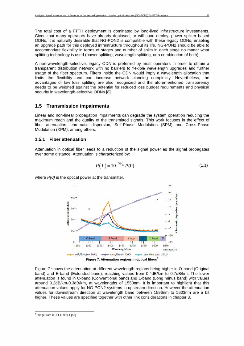
Additionally, the use of coherent detection in ud-WDM is been justified because it has many advantages such us increasing sensitivity, extending reach, increasing network capacity by close wavelength allocation, allowing for dispersion compensation or demodulation of advanced modulation formats. However in the case of study (NG-PON2), the implementation of a hybrid architecture that combines TDM and WDM capabilities, permits an increase in the number of users to be served as well as the amount of bandwidth due to the multiplexing of four or eight channels to achieve an aggregated bandwidth of 40Gbit/s or 80Gbit/s. The ONU and OLT requirements are specified in the ITU-T G989 standard as well as the ODN architecture.
Figure 6. Next-generation PON (NG-PON) stages and evolution
3
At this point it is important to highlight that the shared infrastructure and the splitting of the information is achieved using a power splitter in combination with a Coexistence Element (CE) to guarantee the compatibility with legacy PON systems. Figure 6 shows the evolution in time and bandwidth capacity of NG-PON systems until the incoming technology, the NG-PON2, defined by FSAN which is next to be standardized by ITU.
2 Image from: [7]
3 Modified from [54]
Analysis of performances and tolerances of the second generation passive optical networks (NG-PON2) for FTTH systems 21
The total cost of a FTTH deployment is dominated by long-lived infrastructure investments. Given that many operators have already deployed, or will soon deploy, power splitter based ODNs, it is naturally desirable that NG-PON2 is compatible with these legacy ODNs, enabling an upgrade path for this deployed infrastructure throughout its life. NG-PON2 should be able to accommodate flexibility in terms of stages and number of splits in each stage no matter what splitting technology is used (power splitting, wavelength splitting, or a combination of both).
A non-wavelength-selective, legacy ODN is preferred by most operators in order to obtain a transparent distribution network with no barriers to flexible wavelength upgrades and further usage of the fiber spectrum. Filters inside the ODN would imply a wavelength allocation that limits the flexibility and can increase network planning complexity. Nevertheless, the advantages of low loss splitting are also recognized and the aforementioned transparency needs to be weighed against the potential for reduced loss budget requirements and physical security in wavelength-selective ODNs [8].
1.5 Transmission impairments
Linear and non-linear propagation impairments can degrade the system operation reducing the maximum reach and the quality of the transmitted signals. This work focuses in the effect of fiber attenuation, chromatic dispersion, Self-Phase Modulation (SPM) and Cross-Phase Modulation (XPM), among others.
1.5.1 Fiber attenuation
Attenuation in optical fiber leads to a reduction of the signal power as the signal propagates over some distance. Attenuation is characterized by:
1010 (0)AL
P L P
(1.1)
where P(0) is the optical power at the transmitter.
Figure 7. Attenuation regions in optical fibers
4
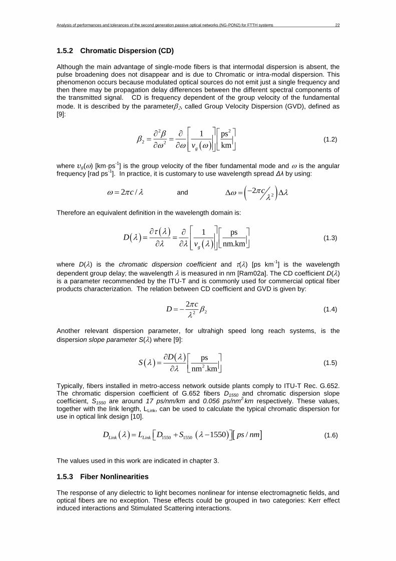
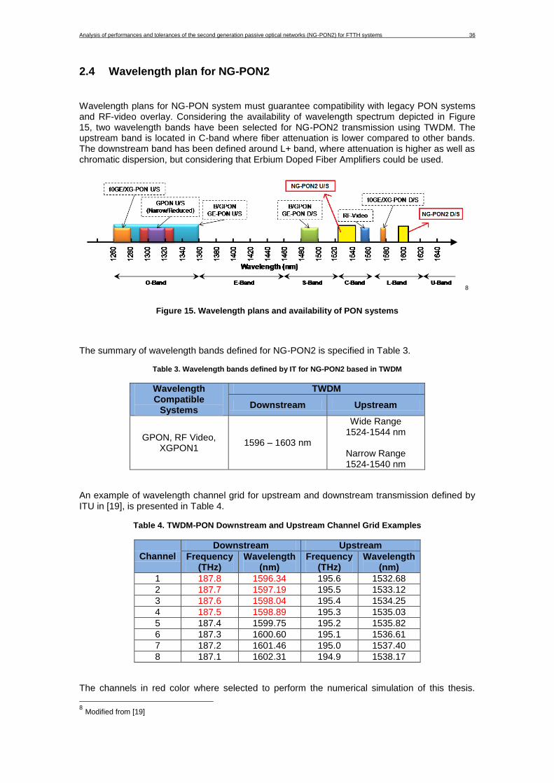
Figure 7 shows the attenuation at different wavelength regions being higher in O-band (Original band) and E-band (Extended band), reaching values from 0.4dB/km to 0.7dB/km. The lower attenuation is found in C-band (Conventional band) and L-band (Long minus band) with values around 0.2dB/km-0.3dB/km, at wavelengths of 1550nm. It is important to highlight that this attenuation values apply for NG-PON2 systems in upstream direction. However the attenuation values for downstream direction at wavelength band between 1596nm to 1603nm are a bit higher. These values are specified together with other link considerations in chapter 3.
4 Image from ITU-T G.989.1
[55]
Analysis of performances and tolerances of the second generation passive optical networks (NG-PON2) for FTTH systems 22
1.5.2 Chromatic Dispersion (CD)
Although the main advantage of single-mode fibers is that intermodal dispersion is absent, the pulse broadening does not disappear and is due to Chromatic or intra-modal dispersion. This phenomenon occurs because modulated optical sources do not emit just a single frequency and then there may be propagation delay differences between the different spectral components of the transmitted signal. CD is frequency dependent of the group velocity of the fundamental
mode. It is described by the parameter, called Group Velocity Dispersion (GVD), defined as
[9]:
2 2
2 2
1 ps
kmgv
(1.2)
where vg() [km·ps-1
] is the group velocity of the fiber fundamental mode and is the angular frequency [rad ps
-1]. In practice, it is customary to use wavelength spread Δλ by using:
2 /c and 22Δ Δc
Therefore an equivalent definition in the wavelength domain is:
1 ps
nm.kmg
Dv
(1.3)
where D() is the chromatic dispersion coefficient and () [ps km-1
] is the wavelength
dependent group delay; the wavelength is measured in nm [Ram02a]. The CD coefficient D() is a parameter recommended by the ITU-T and is commonly used for commercial optical fiber products characterization. The relation between CD coefficient and GVD is given by:
22
2 cD
(1.4)
Another relevant dispersion parameter, for ultrahigh speed long reach systems, is the
dispersion slope parameter S() where [9]:
2
ps
nm .km
DS
(1.5)
Typically, fibers installed in metro-access network outside plants comply to ITU-T Rec. G.652. The chromatic dispersion coefficient of G.652 fibers D1550 and chromatic dispersion slope coefficient, S1550 are around 17 ps/nm/km and 0.056 ps/nm
2.km respectively. These values,
together with the link length, LLink, can be used to calculate the typical chromatic dispersion for use in optical link design [10].
1550 1550 1550 /Link LinkD L D S ps nm (1.6)
The values used in this work are indicated in chapter 3.
1.5.3 Fiber Nonlinearities
The response of any dielectric to light becomes nonlinear for intense electromagnetic fields, and optical fibers are no exception. These effects could be grouped in two categories: Kerr effect induced interactions and Stimulated Scattering interactions.
Analysis of performances and tolerances of the second generation passive optical networks (NG-PON2) for FTTH systems 23
1.5.3.1 Kerr-like non-linear interactions
The physical origin of this effect lies in the anharmonic response of electrons to optical fields and affects the refractive index inside the fiber. Mathematically it is described by:
0 2 0 2 eff
Pn n n I n n
A
(1.7)
where n0 is the linear refractive index of silica glass, n2 is the non-linear index coefficient, P is the power of the beam and Aeff is the effective area of its transverse section. The numerical value accepted for n2 is about 2.6 x 10
-20 m
2/W.
The general propagation equation that includes the effects of dispersion and nonlinearities can be described by the NLSE (Nonlinear Scrödinger Equation):
2 32
2 32 3
A i A 1 A 1β β αA iγ A A
z 2 t 6 t 2
(1.8)
where are the fiber losses and is an important nonlinear parameter with values ranging from 1 to 5 W
-1/km and is described by:
2
0
2 1
km Weff
n
A
(1.9)
Self-Phase Modulation
The intensity-dependent refractive index causes an intensity-dependent phase shift in the fiber. If the optical beam is modulated, the optical intensity depends on time and therefore also the refractive index of the medium becomes time-dependent. Thus an arbitrary wave propagating in a Kerr medium experiences self-induced spurious phase modulation. When a single optical beam propagates in the medium this phenomenon is known as Self Phase Modulation (SPM). In absence of dispersion the generalized NLSE equation (1.11) assumes the form:
2A
2
Ai A A
z
which can be integrated directly to give [11]:
2
0( , ) (0, ) [ | (0, ) | ] (0, ) [ ( ) ]e eA L t A t exp i A t L ff A t exp i P t L ff
(1.10)
where P0(t) is the input power temporal profile and
1
1 L
effL e
(1.11)
is the effective length, taking into account the power decay due to fiber attenuation. The
maximum phase shift is given by . For a conventional single mode fiber the
limit value for Leff is about 21 km ( = 0.2 dB/km), beyond this length nonlinear effects are
negligible. [9]
A time dependent phase implies a frequency shift with the magnitude ( ) NLdt
dt
concluding that SPM leads to chirping of optical pulses manifest through broadening of the pulse spectrum.
Analysis of performances and tolerances of the second generation passive optical networks (NG-PON2) for FTTH systems 24
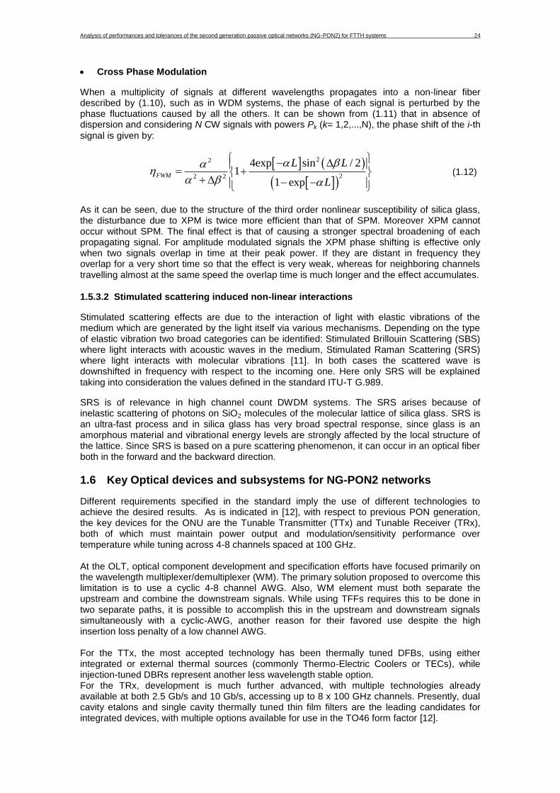
Cross Phase Modulation
When a multiplicity of signals at different wavelengths propagates into a non-linear fiber described by (1.10), such as in WDM systems, the phase of each signal is perturbed by the phase fluctuations caused by all the others. It can be shown from (1.11) that in absence of dispersion and considering N CW signals with powers Pk (k= 1,2,...,N), the phase shift of the i-th
signal is given by:
22
22 2
4exp sin / 21
1 expFWM
L L
L
(1.12)
As it can be seen, due to the structure of the third order nonlinear susceptibility of silica glass, the disturbance due to XPM is twice more efficient than that of SPM. Moreover XPM cannot occur without SPM. The final effect is that of causing a stronger spectral broadening of each propagating signal. For amplitude modulated signals the XPM phase shifting is effective only when two signals overlap in time at their peak power. If they are distant in frequency they overlap for a very short time so that the effect is very weak, whereas for neighboring channels travelling almost at the same speed the overlap time is much longer and the effect accumulates.
Stimulated scattering effects are due to the interaction of light with elastic vibrations of the medium which are generated by the light itself via various mechanisms. Depending on the type of elastic vibration two broad categories can be identified: Stimulated Brillouin Scattering (SBS) where light interacts with acoustic waves in the medium, Stimulated Raman Scattering (SRS) where light interacts with molecular vibrations [11]. In both cases the scattered wave is downshifted in frequency with respect to the incoming one. Here only SRS will be explained taking into consideration the values defined in the standard ITU-T G.989.
SRS is of relevance in high channel count DWDM systems. The SRS arises because of inelastic scattering of photons on SiO2 molecules of the molecular lattice of silica glass. SRS is an ultra-fast process and in silica glass has very broad spectral response, since glass is an amorphous material and vibrational energy levels are strongly affected by the local structure of the lattice. Since SRS is based on a pure scattering phenomenon, it can occur in an optical fiber both in the forward and the backward direction.
1.6 Key Optical devices and subsystems for NG-PON2 networks
Different requirements specified in the standard imply the use of different technologies to achieve the desired results. As is indicated in [12], with respect to previous PON generation, the key devices for the ONU are the Tunable Transmitter (TTx) and Tunable Receiver (TRx), both of which must maintain power output and modulation/sensitivity performance over temperature while tuning across 4-8 channels spaced at 100 GHz. At the OLT, optical component development and specification efforts have focused primarily on the wavelength multiplexer/demultiplexer (WM). The primary solution proposed to overcome this limitation is to use a cyclic 4-8 channel AWG. Also, WM element must both separate the upstream and combine the downstream signals. While using TFFs requires this to be done in two separate paths, it is possible to accomplish this in the upstream and downstream signals simultaneously with a cyclic-AWG, another reason for their favored use despite the high insertion loss penalty of a low channel AWG. For the TTx, the most accepted technology has been thermally tuned DFBs, using either integrated or external thermal sources (commonly Thermo-Electric Coolers or TECs), while injection-tuned DBRs represent another less wavelength stable option. For the TRx, development is much further advanced, with multiple technologies already available at both 2.5 Gb/s and 10 Gb/s, accessing up to 8 x 100 GHz channels. Presently, dual cavity etalons and single cavity thermally tuned thin film filters are the leading candidates for integrated devices, with multiple options available for use in the TO46 form factor [12].
Analysis of performances and tolerances of the second generation passive optical networks (NG-PON2) for FTTH systems 25
1.6.1 Optical Transmitters
TWDM–PON OLT requires tunable transmitters to serve different Optical Distribution Networks (ODNs) using TDM access schemes in order to balance the traffic load. Tunable OLT transmitters consisting of multiple transceivers, instead of a single tunable transceiver, can be added to the TWDM PON system for incremental bandwidth upgrade with wavelength granularity [13]. The OLT transmitter consist of four stacked EML (External Modulated Lasers), each modulated at Gb/s, external AM modulators and WDM mux to combine different wavelengths before feeding the trunk fiber.
1.6.1.1 Laser Characteristics Laser characteristics, e.g. spectral linewidth, relative intensity noise (RIN), Side mode suppression ratio (SMSR), frequency chirp and extinction ratio, are very important parameters that affects the behavior of the transmission. Some of this parameters are fixed using typical DFB values to run the system simulations, like it will be shown in chapter 3.
Spectral linewidth
Laser emits more than one light beam, so the spectral linewidth or simply linewidth corresponds to the Full Width of Half of Maximum (FWHM)(unmodulated) of the lorentzian curve that characterize the spectral response or the point where the power is at least half the maximum or have suffer -3dB of attenuation. More precisely, it is the width of the power spectral density of the emitted electric field in terms of frequency, wavenumber or wavelength.
The linewidth of a laser depends strongly on the type of laser. It may be further minimized by optimizing the laser design and suppressing external noise influences as far as possible. Also it can be reduced by increasing cavity length L and power P. For typical DFB semiconductor lasers, the value of linewidth varies between 5-10 MHz. However Multi-Quantum Well (MQW) DFB lasers are found to exhibit a linewidth as small as 270 KHz at a power of 13.5 mW [14].
Relative Intensity Noise (RIN)
It refers to intensity fluctuations in the laser output caused by reflections from fiber splices and connectors in the link. In semiconductor lasers, output optical power may fluctuate due to the existence of spontaneous emission, thus producing intensity noise. RIN is a function of frequency and increase when power increases. RIN is defined as [15]:
2
( )P
opt
SRIN
P
(1.13)
where Sp(𝜔) is the intensity noise power spectral density and Popt is the total optical power.
Side Mode Suppression Ratio (SMSR)
Single-longitudinal mode oscillation can be achieved by using a filtering mechanism in the laser that selects the desired wavelength and provides loss at the other wavelengths. An important attribute of such a laser is its side-mode suppression ratio, which determines the level to which the other longitudinal modes are suppressed, compared to the main mode. This ratio is typically more than 30 dB for practical SLM lasers [16].
Frequency Chirp
The direct modulation of semiconductor lasers can cause a dynamic shift of the peak wavelength emitted from the device. This phenomenon, which results in dynamic linewidth broadening under the direct modulation of the injection current, is referred to as frequency chirping.
Analysis of performances and tolerances of the second generation passive optical networks (NG-PON2) for FTTH systems 26
It arises from gain-induced variations in the laser refractive index due to the strong coupling between the free carrier density and the index of refraction which is present in any semiconductor structure. In a simple model the chirp-induced power penalty is given by [9]:
(1.14)
where Δλc is the spectral shift associated with frequency chirping.
1.6.1.2 Optical modulators
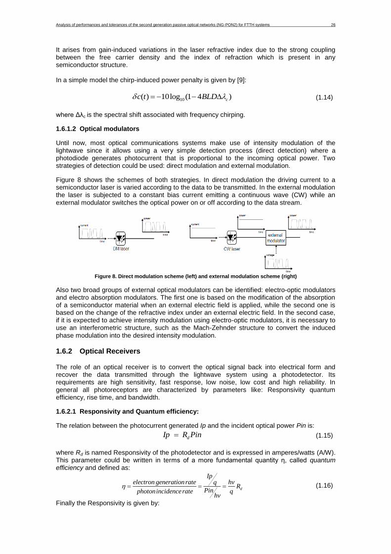
Until now, most optical communications systems make use of intensity modulation of the lightwave since it allows using a very simple detection process (direct detection) where a photodiode generates photocurrent that is proportional to the incoming optical power. Two strategies of detection could be used: direct modulation and external modulation.
Figure 8 shows the schemes of both strategies. In direct modulation the driving current to a semiconductor laser is varied according to the data to be transmitted. In the external modulation the laser is subjected to a constant bias current emitting a continuous wave (CW) while an external modulator switches the optical power on or off according to the data stream.
Figure 8. Direct modulation scheme (left) and external modulation scheme (right)
Also two broad groups of external optical modulators can be identified: electro-optic modulators and electro absorption modulators. The first one is based on the modification of the absorption of a semiconductor material when an external electric field is applied, while the second one is based on the change of the refractive index under an external electric field. In the second case, if it is expected to achieve intensity modulation using electro-optic modulators, it is necessary to use an interferometric structure, such as the Mach-Zehnder structure to convert the induced phase modulation into the desired intensity modulation.
1.6.2 Optical Receivers
The role of an optical receiver is to convert the optical signal back into electrical form and recover the data transmitted through the lightwave system using a photodetector. Its requirements are high sensitivity, fast response, low noise, low cost and high reliability. In general all photoreceptors are characterized by parameters like: Responsivity quantum efficiency, rise time, and bandwidth.
1.6.2.1 Responsivity and Quantum efficiency:
The relation between the photocurrent generated Ip and the incident optical power Pin is:
dIp R Pin (1.15)
where Rd is named Responsivity of the photodetector and is expressed in amperes/watts (A/W). This parameter could be written in terms of a more fundamental quantity η, called quantum efficiency and defined as:
d
Ipelectron generationrate hvq
RPinphotonincidencerate q
hv
(1.16)
Finally the Responsivity is given by:
10( ) 10log (1 4 )cc t BLD
Analysis of performances and tolerances of the second generation passive optical networks (NG-PON2) for FTTH systems 27
1.24Rd
hv
(1.17)
As can be seen, the Responsivity depends linearly of the wavelength λ until a certain limit where the quantum efficiency η drops to zero. This occurs at λc (cutoff wavelength) and varies
according to the semiconductor material which presents different absorption coefficients (α).
1.6.2.2 Noise in Photodetectors
The most important characteristic in any receiver is the receiver sensitivity defined as the minimum optical power required to achieve a specific Bit Error Rate (BER). Receiver sensitivity depends on the Signal to Noise Ratio (SNR), which also depends on several noise sources that distort the received signal. Three of these noise sources are: shot noise, thermal noise and the dark current.
Shot noise is an essential noise generated by the behavior of the induced carriers and incident photons as particles. The motion of generated carriers is random and converted to photocurrent fluctuations as shot noise. The mean-square shot noise current in a determinate bandwidth is given by:
2 2sn PqI Bw (1.18)
Thermal noise is a spontaneous fluctuation due to thermal interaction between the free electrons and the vibrating ions in a conducting medium, and it is especially prevalent in resistors at room temperature. The thermal noise current it in a load resistor RL may be expressed by its mean square value and is given by:
2 4 nt
L
KTBF
R (1.19)
where K is Boltzmann’s constant, Fn is the Noise Factor transimpedance amplifier, T is the absolute temperature and B is the post-detection (electrical) bandwidth of the system (assuming the resistor is in the optical receiver)
5.
Dark current noise is a small reverse leakage current that still flows from the device terminal when there is no optical power incident. The dark current noise is given by:
2 2d qBId
(1.20)
1.6.2.3 Signal to Noise Ratio (SNR)
The signal to noise ratio is defined after the photodetector as the ratio between the received power and the noise power generated through the link plus the noise generated as consequence of photodetection process.
S Psignal
SNR dBN Pnoise
(1.21)
where P is average power. Both signal and noise power must be measured at equivalent points in a system, and within the same system bandwidth.
PIN photodiodes (Possitive intrinsic Negative)
This class of photodiodes doesn’t have internal gain. The two main sources of noise in photodiodes without internal gain are dark current noise and quantum noise. The SNR for the PIN photodiode receiver may be obtained by summing the noise contributions. It is given by:
5 Page 503, [37]
Analysis of performances and tolerances of the second generation passive optical networks (NG-PON2) for FTTH systems 28
2
42 ( ) n
p d
L
IpSNR
KTBFqB I I
R
(1.22)
where Fn is the noise figure related with the amplifiers and typically
In PIN photodiodes thermal noise dominates the receiver performance, so shot noise and dark current contribution can be neglected obtaining the thermal noise limit case:
2 2
4
L
n
R R PinSNR
KTBF (1.23)
APD (Avalanche Photodiode)
Optical receivers that employ an APD generally provide a higher SNR for the same incident optical power due to the internal gain that increases the photocurrent by a factor M:
(1.24)
Thermal noise remains the same for APD receivers, as it originates in the electrical components that are not part of the APD. However, the dark current and quantum noise are increased by the multiplication process and may become a limiting factor. Total shot noise will result in:
2 2sn PqI Bw (1.25)
And the corresponding SNR will be: 2 2
2 42 ( ) ( ) n
p d A
L
M IpSNR
KTBFqB I I M F M
R
(1.26)
where FA is the excess noise factor of the APD and is given by [86]:
1( ) ( )( )2 1/A A AF M k M k M (1.27)
where KA is the ionization coefficient ratio defined as:
or defined such that 0 < k 1A h e h e Ak (1.28)
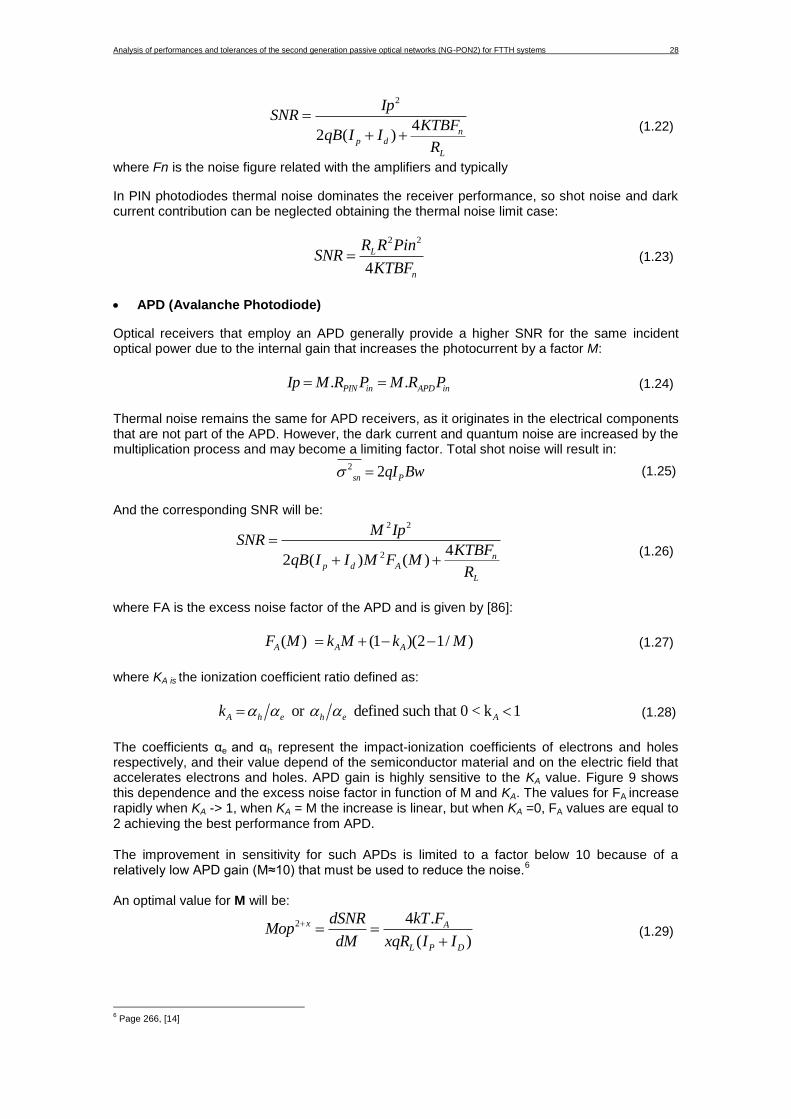
The coefficients αe and αh represent the impact-ionization coefficients of electrons and holes respectively, and their value depend of the semiconductor material and on the electric field that accelerates electrons and holes. APD gain is highly sensitive to the KA value. Figure 9 shows this dependence and the excess noise factor in function of M and KA. The values for FA increase rapidly when KA -> 1, when KA = M the increase is linear, but when KA =0, FA values are equal to 2 achieving the best performance from APD.
The improvement in sensitivity for such APDs is limited to a factor below 10 because of a relatively low APD gain (M≈10) that must be used to reduce the noise.
6
An optimal value for M will be:
2 4 .
( )
x A
L P D
kT FdSNRMop
dM xqR I I
(1.29)
6 Page 266, [14]
. .PIN in APD inIp M R P M R P
Analysis of performances and tolerances of the second generation passive optical networks (NG-PON2) for FTTH systems 29
where x is between 0.3 and 0.5 for silicon APDs and between 0.7 and 1.0 for germanium or III–V alloy APDs.
Figure 9. Excess noise factor FA as an function of the average APD gain M for several values of KA
1.6.3 Optical Tunable Filters, WDM MUX and DEMUX.
WDM systems require a set of components that permits the transmission of multiple optical channels over the same fiber. Tunable optical filters are the most basic components for selecting a specific channel in a system that requires tunable receivers, as is the case of NG-PON2 systems. Different effects appear due to non-ideal filter transmission function causing some optical energy of the neighboring channels to leak through the filter, causing interchannel crosstalk that could be minimized increasing the spectral separation between channels, however different standardizations have been made for CWDM and DWDM channels restricting the channel spacing to 10nm and 1nm approximately.
A tunable optical filter should have a wide tuning range, lower crosstalk to avoid interference from adjacent channels, fast tuning speed, small insertion loss, stability against environmental changes, insensitivity to signal polarization and lower cost. Different kind of optical filters have been considered as NG-PON2 solutions: Fiber Perot filter (etalon filters), Mach Zhender interferometers, thin-film filters and Fiber Bragg Grating (FBG).
1.6.3.1 Fiber-Perot Filters (Etalon):
It consists of a single cavity formed by two parallel mirrors. A specific wavelength can be selected adjusting the distance between the mirrors according to [17] :
(2 cos ) /m cnL m (1.30)
where n is the etalon reflective index and Lc is its length. The transfer function of an FP filter whose mirrors have the same reflectivity Rm is:
(1 )( )
1 exp( )
i
mf
m r
R eH
R i
(1.31)
Where 2 /r f gL is the round-trip time inside the filter. These filters are characterized by
two parameters: Free Spectral Range (FSR) and finesse. FSR makes reference to the period after the transfer function or filter shape repeats itself and when the values are maximum. The FSR correspond with:
/
2
c nFSR
L
(1.32)
The finesse is a measure of the width of the filter transfer function and is a parameter of quality of the filter. Mathematically it can be expressed as the relation between the FSR and the channel bandwidth at -3dB:
Analysis of performances and tolerances of the second generation passive optical networks (NG-PON2) for FTTH systems 30
FSRFinesse
BW (1.33)
1.6.3.2 Mach Zehnder filter
This filter can be constructed by connecting the two output ports of a 3-dB coupler to the two inputs of another 3-dB coupler. In a first stage the signal is split in two equal parts which suffer different phase shifts (one arm of MZ structure are made with more fiber than the other) before they interfere at the second coupler. This phase shift is wavelength dependent converting the MZ interferometer in an optical filter. This kind of filter is a low cost device but the tuning time is high (miliseconds) as well as insertion losses. The number of channels is limited to 8. [18].
The transfer function of a Mach Zehnder filter is:
2
2 1( ) cos ( )n
T f l l fc
(1.34)
where l1 and l2 are the lengths of each arm of the MZ interferometer, and FSR and the parameter characteristics are:
2 1( )
cFSR
n l l
2 12 ( )
cBW
n l l
2F
1.6.3.3 Thin film filter
A thin-film resonant cavity filter (TFF) is a Fabry-Perot interferometer where the mirrors surrounding the cavity are made by using multiple reflective dielectric thin-film layers. This device acts passing through a particular wavelength (determined by the cavity length) and reflecting all the other wavelengths. A thin-film resonant multicavity filter (TFMF) consists of two or more cavities separated by reflective dielectric thin-film layers. As more cavities are added, the top of the passband becomes flatter and the skirts become sharper. In order to obtain a multiplexer or a demultiplexer, a number of these filters can be cascaded. Each filter passes a different wavelength and reflects all the others passes one wavelength and reflects all the others onto the second filter. The second filter passes another wavelength and reflects the remaining ones, and so on [16]. Some interesting characteristics of this kind of filters are their very flat top on the passband and very sharp skirts, stability to temperature variations, low loss and insensitively to the polarization of the signal. In terms of disadvantages, since TFF are free-space devices, precise collimation of optical beams is required and the difficulty becomes significant when the channel count is high.
1.6.3.4 AWG.
Arrayed Waveguide Grating (AWG) is another configuration to make mux, demux, and add/drop coupler and is based on planar lightwave circuit (PLC) technology in which multipath interference is utilized through multiple waveguide delay lines. For applications involving large numbers of channels, such as 64 and 128, AWGs are more appropriate than TFFs since an AWG has lower loss and flatter passband, and is easier to realize on an integrated-optic substrate. In TFFs the required number of cascaded thin film units is equal to the number of wavelength channels, therefore insertion loss linearly increases with the number of ports and the optical alignment accuracy requirement becomes more stringent. For example in an AWG demultiplexer the incoming WDM signal is coupled into an array of planar waveguides after passing through the first star coupler. In each waveguide, the WDM signal experiences a different phase shift due to the different length of waveguides such that the phase difference between two neighboring waveguides is constant. The phase-shift is also wavelength-dependent because it depends on the mode-propagation constant. At the end when light passes through the second star coupler different channels focus to different output waveguides, resulting in a WDM signal demultiplexed into individual channels.
Analysis of performances and tolerances of the second generation passive optical networks (NG-PON2) for FTTH systems 31
CHAPTER 2. Next Generation PON(NG-PON) standards
With the increase in broadband services demand many PON technologies have been proposed to provide broadband optical access beyond 10 Gbit/s. Wavelength Division Multiplexed PON (WDM-PON)[1], Optical Code Division Multiple Access PON (OCDMA-PON)[2], Orthogonal Frequency Division Multiplexed PON (OFDM-PON)[3], as well as Time and Wavelength Division Multiplexed PON (TWDM-PON)[4] have been considered. However TWDM-PON has been selected due to attracted considerable support from global vendors in the Full Service Access Network (FSAN) community. It increases the aggregate PON rate by stacking 4x10 XG-PON pairs of wavelengths to provide 40Gb/s and 10Gb/s in downstream and upstream, respectively
2.1 NG-PON2 ITU-T G.989 Recommendation
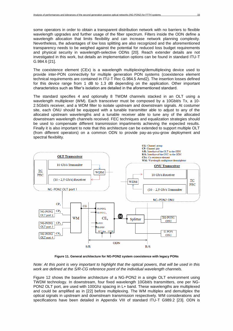
The requirements of the next generation PON stage 2 (NGPON2) that is been standardized by ITU should enable flexible deployment options to fit operator needs and engineering choices such as providing a modular way to aggregated capacity as service demands grow or as spectrum is vacated by the existence of legacy PON systems. The system should allow different customer types (business, residential, etc) in the same scenario, each one requiring different demands. However, minimum guidelines have to be defined and standardized to serve as reference in the future deployment. The standard ITU-T G.989 will provide a complete set of requirements which describe 40-Gigabit-capable passive optical network (NG-PON2) systems in an optical access network for residential, business, mobile backhaul and other applications. The complete NG-PON2 standard is expected for 2015 and it will be divided as follows:
Recommendation ITU-T G.989.1 presents the general requirements, in order to guide and motivate the physical layer and the transmission convergence layer specifications. This Recommendation includes principal deployment configurations, migration scenarios from legacy PON systems, and system requirements. Also it includes the service and operational requirements to provide a robust and flexible optical access network supporting all access applications.
Recommendation ITU-T G.989.2. will present the physical layer specifications for the NG-PON2 physical media dependent (PMD) layer.
Recommendation ITU-T G.989.3 will describe the transmission convergence (TC) layer
Finally the ONU management and control interface (OMCI) specifications are described in
Recommendation ITU-T G.988 for NG-PON2 extensions [19]. This thesis will analyze in depth the recommendations G989.1 and G89.2 in order to meet the minimum requirements to take as reference for performing the architecture simulations.
2.2 System Overview and NG-PON2 trade-offs
As it is defined in [19] a TWDM-PON (Time and Wavelength Division Multiplexing Passive Optical Network) is a multiple wavelength PON solution in which each wavelength is shared between multiple optical network units (ONUs) by employing time division multiplexing (TDM) and multiple access mechanisms.
Although the basic architecture of NG-PON2 consist on 4x10 Gb/s TWDM channels, with OLTs and ONUs of 10Gb/s transmitter and 2.5 Gb/s receiver ports some alternative solutions have been detailed in NG-PON2 standard in order to give flexibility for balancing the trade-offs in speed, distance and split ratios for various applications.
NG-PON2 systems include support for:
• 4-8 TWDM channel pairs -> not all need to be active -> “pay as you grow”
Analysis of performances and tolerances of the second generation passive optical networks (NG-PON2) for FTTH systems 32
• Downstream and upstream nominal line rates per channel:
• 40 km of fiber reach and configurable differential fiber distance (20-40km)
• 60 km of fiber reach with passive outside plant • 1:256 split ratio
Note: An ONU is characterized by its fiber distance, and for each pair of ONUs on the same OLT PON interface, the differential fiber distance is the difference between the two individual fiber distances as depicted in Figure 10
Figure 10. Differential distance concept7
The set of parameter combinations that are supported by the system is summarized in Table 2.
Table 2. NG-PON2 splitting ratio options
Distance (km)
Bit Rate (Gb/s)
Number of users
Down/Up Down/Up
10/2.5 10/10
Split Ratio
20 64 256
40 32 128
With these splitting ratios it is expected that the PON can provide services at least to 256 users in the case of 64-splitting ratio, taking into account that each wavelength channel could serve 64 users.
2.3 NG-PON2 architecture
Figure 11 depicts an NG-PON2 scenario and reference points to guarantee coexistence with legacy PON systems. The Optical Distribution Network (ODN) consists of the power splitter and the coexistence element (WDM) and optionally reaches extenders.
Power splitter based ODNs permits to operators deploy FTTH systems with long-lived infrastructure investments. Moreover, a non-wavelength-selective, legacy ODN is preferred by
7 Figure from ITU-T G.987 standard [19]
Analysis of performances and tolerances of the second generation passive optical networks (NG-PON2) for FTTH systems 33
some operators in order to obtain a transparent distribution network with no barriers to flexible wavelength upgrades and further usage of the fiber spectrum. Filters inside the ODN define a wavelength allocation that limits flexibility and can increase network planning complexity. Nevertheless, the advantages of low loss splitting are also recognized and the aforementioned transparency needs to be weighed against the potential for reduced loss budget requirements and physical security in wavelength-selective ODNs [20]. Reach extender details are not investigated in this work, but details an implementation options can be found in standard ITU-T G.984.6 [21].
The coexistence element (CEx) is a wavelength multiplexing/demultiplexing device used to provide inter-PON connectivity for multiple generation PON systems (coexistence element technical requirements are contained in ITU-T Rec G.984.5 Amd2). The insertion losses defined for this device range from 1 dB to 1.3 dB depending on the application. Other important characteristics such as filter’s isolation are detailed in the aforementioned standard.
The standard specifies 4 and optionally 8 TWDM channels stacked in an OLT using a wavelength multiplexer (WM). Each transceiver must be composed by a 10Gbit/s Tx, a 10-2.5Gbit/s receiver, and a WDM filter to isolate upstream and downstream signals. At costumer site, each ONU should be equipped with a tunable transmitter able to adjust to any of the allocated upstream wavelengths and a tunable receiver able to tune any of the allocated downstream wavelength channels received. FEC techniques and equalization strategies should be used to compensate different transmission impartments achieving the expected results. Finally it is also important to note that this architecture can be extended to support multiple OLT (from different operators) on a common ODN to provide pay-as-you-grow deployment and spectral flexibility.
Figure 11. General architecture for NG-PON2 system coexistence with legacy PONs
Note: At this point is very important to highlight that the optical powers, that will be used in this work are defined at the S/R-CG reference point of the individual wavelength channels.
Figure 12 shows the baseline architecture of a NG-PON2 in a single OLT environment using TWDM technology. In downstream, four fixed wavelength 10Gbit/s transmitters, one per NG-PON2 OLT port, are used with 100Ghz spacing in L+ band. These wavelengths are multiplexed and could be amplified as in [22] before multiplexing. The WM multiplex and demultiplex the optical signals in upstream and downstream transmission respectively. WM considerations and specifications have been detailed in Appendix VIII of standard ITU-T G989.2 [23]. ODN is
Analysis of performances and tolerances of the second generation passive optical networks (NG-PON2) for FTTH systems 34
composed by up to 40 km of SMF (ITU-T G.652 OR compatible) with specific attenuation and dispersion characteristics described in chapter 3. NG-PON2 ODN specifies bidirectional transmission using 1 fiber WDM with two different wavelength channels (UP/DOWN). A power splitter is required to broadcast the transmitted signal to each ONU through drop fibers. The ONU could be located as maximum with a differential distance of 40 km and configurable in the range (20 km – 40 km) The PON should support at least 256 users that could be served using a power splitter of 1:64 splitting ratio. Finally, at the ONU another WDM filter isolates the upstream and downstream signals and a tunable filter should be used to select a specific wavelength that will be detected for a 10Gbit/s PIN or APD photodiode. After the photodetection a Low Pass Filter (LPF) will be used to reduce the noise generated by trans-impedance amplifier.
In upstream transmission the ONU Tx should be a tunable device (Thermally DFB lasers, VCSEL, DBR, etc) to transmit at different wavelengths. This could be achieved using different techniques and technologies as explained in chapter 1. The signal goes through the WDM filter to the ODN where it is multiplex again by the splitter and after 40 km of SMF is filtered by the WM, preamplified and demultiplexed inside the OLT.
Figure 12. Detailed architecture of a TWDM-PON
Note: The setup tested in this work does not have neither pre-amplifiers, nor in-line amplifiers, nor boost amplifiers. Moreover the setup tested only considers the downstream transmission as it will be explained in chapter 3.
It is also important to know in detail the configuration of the transceiver at OLT and ONU. The OLT transceiver is depicted in Figure 13. The transceiver is provided with a 10Gbit/s Tx, a 10-2.5 Gbit/s Rx and a WDM filter separates the upstream and downstream signals. The Tx could be designed with an External Modulated Laser (EML) using a MZM, a Direct Modulated Laser or an Electro Absortion Modulator Laser (EAM) conformed by a DFB attached to the AM modulator in the same device which is fixed at a specific wavelength and which will be modulated by an NRZ electrical signal at the AM modulator. The option selected in the VPI setup is explained in chapter 3. The transceivers are composed by 4 EML lasers that are
Analysis of performances and tolerances of the second generation passive optical networks (NG-PON2) for FTTH systems 35
multiplexed (and optionally amplified [24]) before arriving to the WDM filter device that could be implemented using an optical circulator or a wavelength filter.
The receiver presents an optional preamplifier (optional), a demultiplexer, the PIN or PAD photoreceiver and the LPF. Additionally equalizers could be used to compensate undesired transmission effects and limiting electrical amplifiers to boost the receiver signal [24]. The VPI option selected will be presented in chapter 3.
Figure 13. OLT Transceiver for NG-PON2
The ONU transceiver scheme explained before is depicted in Figure 14.
Figure 14. ONU Transceiver for NG-PON2
It is important here to highlight that both receiver and transmitter should be tunable to meet the NG-PON2 requirements.
Analysis of performances and tolerances of the second generation passive optical networks (NG-PON2) for FTTH systems 36
2.4 Wavelength plan for NG-PON2
Wavelength plans for NG-PON system must guarantee compatibility with legacy PON systems and RF-video overlay. Considering the availability of wavelength spectrum depicted in Figure 15, two wavelength bands have been selected for NG-PON2 transmission using TWDM. The upstream band is located in C-band where fiber attenuation is lower compared to other bands. The downstream band has been defined around L+ band, where attenuation is higher as well as chromatic dispersion, but considering that Erbium Doped Fiber Amplifiers could be used.
8
Figure 15. Wavelength plans and availability of PON systems
The summary of wavelength bands defined for NG-PON2 is specified in Table 3.
Table 3. Wavelength bands defined by IT for NG-PON2 based in TWDM
Wavelength Compatible
Systems
TWDM
Downstream Upstream
GPON, RF Video, XGPON1
1596 – 1603 nm
Wide Range 1524-1544 nm
Narrow Range 1524-1540 nm
An example of wavelength channel grid for upstream and downstream transmission defined by ITU in [19], is presented in Table 4.
Table 4. TWDM-PON Downstream and Upstream Channel Grid Examples
Channel
Downstream Upstream
Frequency (THz)
Wavelength (nm)
Frequency (THz)
Wavelength (nm)
1 187.8 1596.34 195.6 1532.68
2 187.7 1597.19 195.5 1533.12
3 187.6 1598.04 195.4 1534.25
4 187.5 1598.89 195.3 1535.03
5 187.4 1599.75 195.2 1535.82
6 187.3 1600.60 195.1 1536.61
7 187.2 1601.46 195.0 1537.40
8 187.1 1602.31 194.9 1538.17
The channels in red color where selected to perform the numerical simulation of this thesis.
8 Modified from [19]
Analysis of performances and tolerances of the second generation passive optical networks (NG-PON2) for FTTH systems 37
2.5 TWDM-PON Physical layer requirements
A series of considerations and parameters define the TWDM-PON architecture and the limits in the upstream and downstream transmission. The following sections will explain how to calculate these limits in terms of the power budget available and other important characteristics.
2.5.1 Power Budget
Power budget (PB) is determined by the Optical Path Losses (OPL, also called link or loss budget) and the optical path penalty. The optical path losses were determined in standard ITU-T G.987.2 for XG-PON systems and applied to NG-PON2 considering that NG-PON2 is obtained multiplexing 4 XG-PON1 signals. The classes of optical path losses determine the ODN classes and the minimum requirements for each one. These classes include losses due to distance attenuation, splitter losses, total connector losses, fusion splice losses and Coexistence Element (CE) losses. Taking this into account the OPL could be obtained by:
S S lossesOPL L CE Splitx ter lossey s (2.1)
Where
α = typical attenuation coefficient of the fiber cables in a link (laboratory environment) L = Fiber length αs = mean splices loss x = number of splices in a link αc = mean loss of line connectors y = number of line connectors in a link (if provided) CElosses= Coexistence element losses Splitter losses=Insertion losses(IL) + Excess losses(EL) + Polarization dependent losses(PDL)
Typical values for splitter losses will be presented in chapter 3. The network dimensioning described in chapter 5 determines the splitter losses in terms of number of users to calculate the power budget available for transmission. The total ODN classes should be lower than the sum of optical losses obtained from Eq. (2.1). The maximum OPL values permitted for each ODN class will be presented in Table 5. The other term that should be considered in the power budget is the Optical Path Penalty (OPP) that includes losses due to dispersion, reflections, jitter and Raman Effect. The maximum OPP values permitted for each ODN classes will also be presented in Table 5. The CE losses (1 – 1.3 dB), as explained earlier, have been specified in standard ITU-T G.984.5 [25]. At the end, the power budget will be:
On the other hand, power budget can also be calculated considering the minimum transmitted power established for each ODN and the receiver sensitivity defined in the ITU-T G989 standard. As a consequence, the power budget would be obtained from:
Power Budget (PB) = Minimum Tx Power - Receiver Sensitivity (2.3)
Table 5 shows the PB as function of the OPP, the OPL, the minimum transmitter powers and the receiver sensitivity at a BER of reference and for channels transmitted in downstream and upstream at two bit rates. Other important parameters can be found in tables 11.4 to 11.7 in the standard ITU-T G.989.2 [23].
Analysis of performances and tolerances of the second generation passive optical networks (NG-PON2) for FTTH systems 38
Table 5. Typical interface parameters ONU and OLT for TWDM [19]
Transmission path
Bit Rate (Gbit/s)
ODN max. Class
OPL (dB)
OPP (dB)
PB (dB)
Min. Tx Power (dBm)
Rx sensitivity
BER
Downstream
10
N1 29
2
31 3
-28 10
-3
(10-5
)
N2 31 33 5
E1 33 35 7
E2 35 37 9
2.5
N1 29
0.5 (1)
29.5 0
-30 10-4
(10
-5)
N2 31 32 2
E1 33 34 4
E2 35 36 6
Upstream
10
N1 29
1.5
30.5 4 -26.5
10-3
(10-5
)
2 -28.5
N2 31 32.5 4 -28.5
2 -30.5
E1 33
2
34.5 4 -31
2 -33
E2 35 36.5 NA NA
4 -33
2.5
N1 29
1
29 4 -26
10-4
(10-5
)
0 -30
N2 31 31 4 -28
0 -32
E1 33
1.5
33 4 -30.5
0 -34.5
E2 35 35 4 -32.5
0 -36.5
The table above defines different parameters for the interfaces of OLT and ONU in a TWDM –PON. The column of the Power Budget (PB) is obtained using the equations 2.2 or 2.3. For each ODN class the standard defines a minimum sensitivity parameter and the associated transmitter power. The BER of reference has been defined in each case for two situations, the worst case (black values) and a conservative case (green values) defined in clause 9.4.1 of ITU-T G.Sup 39 recommendation [26].
In the case of downstream transmission the standard has defined two values of OPL. The first one (black color) corresponds with the value for the class N1 without FEC. The second value (blue color) applies for the other ODN classes which uses FEC.
Finally the red values in the table correspond with a situation when in the OLT a pre-amplifier is placed in order to increase the power budget of the transmission.
2.5.2 NG-PON2 experimental setups based on TWDM-PON architectures
The objective of this section is to show a summary of different experimental setups performed by different providers, in order to meet the considerations taken into account in real test, to verify the tolerances and performances in terms of BER, fiber reach and number of users of TWDM-PON architecture. The technologies used, the devices and some parameters of the setups are shown. More information about these tests has been summarized in the annexes and is referenced properly.
Experimental test from recognized vendors as ALCATEL, HUAWEI, ZTE, NTT or MITSUBISHI were studied. In the following two of the most interesting papers are discussed and compared.
Analysis of performances and tolerances of the second generation passive optical networks (NG-PON2) for FTTH systems 39
Table 6. Characteristic parameters of two experimental setups of TWDM-PON
Parameter
Paper 2 - Pd4.F.4 - ECOC 2013 Paper 7- Tu.2.C.6 - OFC 2014
World’s First Demonstration of Pluggable Optical Transceiver
Modules for Flexible TWDM PONs -> Huawei Tech. (F.Effenberger)
Demostration of 10G Burst-Mode DML and EDC in Symmetric 40 Gbit/s TWDM-PON over 40km
Passive Reach -> ZTE Corporation
Value Alternatives - Notes Value Alternatives - Notes
Agregated BW (Gb/s)
40 – 10 4 x 10 Gb/s ; 4 x 2,5
Gb/s 40 - 40
4 x 10 Gb/s ; 4 x 10 Gb/s
Bit rate per channel (Gb/s)
10 / 2,5 Dowstream/ Upstream
10 / 10 Dowstream/ Upstream
Transmission OLT Parameters (Downstream)
Laser Type Dowstream
DFB lasers DFB+EAM
(EML) EML DFB+EA
Modulation format OLT
IM
IM -
Modulation system OLT
EML 4 x EML External -
OLT Tx Power - Máx (dBm) (per
channel at CG point
+10,0 at 10 Gb/s
+7,0 +9,0
+11,0 +11,0
N1 N2 E1 E2
OLT Tx Power - Min (dBm) (per
channel at CG point
- -
+3,0 +5,0 +7,0 +9,0
N1 N2 E1 E2
Extinction Ratio OLT (dB)
9 - 8.2 -
Line code Downstream
(OLT) - - NRZ -
Transmission ONU Parameters (Upstream)
Laser Type Upstream
DFB Thermally tunned DFB
Thermally tuned C-band lasers with
temperature controlled by TEC
Modulation format ONU
IM
IM -
Modulation system ONU
Direct lasers DFB Direct -
ONU Tx Power - Máx (dBm) (per
channel) +4,0 at 10 Gb/s
+7,0 +9,0
+11,0 +11,0
N1 N2 E1 E2
ONU Tx Power - Min (dBm) (per
channel) - -
+3,0 +5,0 +7,0 +9,0
N1 N2 E1 E2
Extinction Ratio ONU (dB)
9 - 6 -
Line code Upstream (ONU)
- - NRZ -
Other ONU considerations
- - * Thin Film Tunable filter (TFF), with
2dB insertion losses and 0.5dB crosstalk penalty
Analysis of performances and tolerances of the second generation passive optical networks (NG-PON2) for FTTH systems 40
Link parameters
Maximum distance tested (km)
40 - 40 -
Split ratio 1:64 Based on We.3.F.6
paper. F.Effenberger - -
Power budget (PB) 36 - - -
Optical Path Penalty (OPP) (dB)
- -
Downstream 2 (all) Upstream 1.5 N1 and 2 (N2,E1 &E2)
Loss budget (link budget) (dB)
- -
14 - 29 16 - 31 18 - 33 20 - 35
N1 N2 E1 E2
Operative wavelenghths
used (nm)
1608,33 1609,19 1610,06 1610,92
1535,82 1536,71 1537,41 1538,19
OLT
ONU
1596,34nm To
1598,89nm
1530,33nm To
1531.90nm
Downstream
Upstream
Channel spacing (GHz)
- - 100 spaced wavelength
grid
Fibers used - - SMF G.652
Dispersion penalty - - 1.1 dB 1.2 dB
20 km 40 km
Other link considerations
WM losses (2 dB) and 0.5 dB crosstalk penalty
CE losses are not considered BM EDC chip contains a 9-tap FFE and 4-tap decision feedback equalizer (DFE)
Receiver Parameters
BER Downstream (without FEC)
10-8->ch1,3,4
10-6->ch2
10
-6->ch 1,3
10
-5->ch 2,4
10
-4>ch1,2,3,4
B2B at Rx Sens. = -26 dBm
20 km at Rx Sens. = -26 dBm 40km, Rx Sens=-26dBm, ch 2 40km Rx Sens=-25 dBm ch4 40km Rx Sens =-26,5 dBm ch 1,3
10-3
-
BER Upstream (without FEC)
10-4
B2B at Rx Sens. = -36 dBm >ch 2,3,4 B2B at Rx Sens. = -36,5 dBm -> ch 1 20km at Rx Sens. = -36 dBm -> ch 1,2,3 20 km at Rx Sens= -36,5 dBm -> ch 4 40 km at Rx Sens. = -36 dBm -> ch 1 40km at Rx Sens. = -35,5 dBm -> ch 2,3 40 km at Rx Sens. = -35 dBm - > ch 4
10-3
-
Analysis of performances and tolerances of the second generation passive optical networks (NG-PON2) for FTTH systems 41
Minimum ONU Rx Power (Sensitivity)
Downstream ONU at 2,5 GB/s
-26 dBm at 20 km. Some channels at 40 km -26,5 with lower VER
- -
Minimum ONU Rx Power (Sensitivity)
Downstream ONU at 10 GB/s
- - -28 dBm -
Minimum OLT Rx Power (Sensitivity).
Upstream OLT at 2,5 GB/s
- - - -
Minimum OLT Rx Power (Sensitivity)
Upstream OLT at 10 GB/s
-36 dBm at 20 km and 40 km
-25.5 dBm -28 dBm -30 dBm -32 dBm
N1 N2 E1 E2
In Table 6, two experimental setups were performed in a TWDM-PON. The first one consists in a demonstration of the first Pluggable Optical Transceiver Module for flexible TWDM PONs developed by HUAWEI [24] with error free. Integrated OLT transceiver in CFP module transmits at 10dBm power and achieves -36dBm sensitivity. Low-cost tunable SFP+ONU with transceiver tuned over 4 channels with 4dBm transmitted power and -26dBm sensitivity was also developed. The second one is a demonstration of a burst-mode 10Gbit/s DML and Electronic Dispersion Compensation (EDC) in a symmetric 40Gbit/s TWDM-PON system over 40 km [27].
To learn about technologies used, it is interesting to know in detail some of the devices used. In the first setup depicted in Figure 16, for the transmitter, 4 EMLs, and optical mux and an integrated L-band EDFA were used. For the receiver a C-band EDFA, and optical demux, burst-mode APD ROSAs and limiting amplifiers (LA) were utilized. Finally a WDM filter that combines/separates upstream/downstream wavelength is placed in the OLT module. The MCU unit control and monitoring purpose (Tx power, Rx power, loss-of-signal alarm).
Figure 16. a) OLT architecture; b) ONU architecture9
In the second setupm [27] for downstream transmission, four fixed wavelength 10Gbit/s EML transmitters at OLT spaced 100GHz are used, and a tunable filter is employed in front of the 10G APD receiver at the ONU. In upstream transmission, 10Gbit/s DML is implemented by employing a direct modulated DFB laser with Temperature Control (TEC). At the OLT site, 10 Gbit/S APD and TIA are used.
As it can be deduced, the preferred strategy for transmit in downstream is the external modulation, while in upstream the most popular technique is the direct modulation due to the low cost requirement at ONU site with the constraint of phenomenon such as chirp and lower extinction ratios.
9 Images from [24]
Analysis of performances and tolerances of the second generation passive optical networks (NG-PON2) for FTTH systems 42
CHAPTER 3. TWDM FOR NG-PON2. VPI SETUP AND DEVICES MODELING
The design of an architecture model based in the reference of the standard and considering cost-efficient components have been configured and simulated in VPIphotonics
TM. Each device
is modelled and the different subsystems (OLT, ONU) described.
To study the performance and tolerances to transmission impairments numerical simulations of a TWDM-PON system have been implemented. VPI simulator is capable to reproduce in detail the architecture described in chapter 2. The focus has been placed on tunable devices (i.e. optical sources and filters) and power splitters which are key component to achieve the best performance of NG-PON2 systems with respect to previous generations.
Characteristics like fiber reach, splitting ratio and tolerance to linear and non-linear impairments have been tested. The general system architecture used throughout this study is shown in Figure 17. Only downstream transmission is considered for reasons explained below.
Figure 17. General system architecture used in the simulations
The OLT, placed in the Central Office, consists of four(4) laser transmitters externally modulated
by means of amplitude intensity modulators (AM) or MZM at wavelengths:
and a device, MUX (AWG or TFF with few dBs losses), to multiplex them into the feeder fiber. The ODN consists of a single-mode fiber feeder and a remote node where the signal is distributed to the ONUs via N drop fibers, generally shorter or much shorter than the feeder fiber. This remote note is a power splitter that is emulated through a variable optical attenuator (VOA) configured with a splitting losses 21.1 dB corresponding to a 1:64 power splitter. Each ONU contains a tunable optical filter that selects a specific wavelength and a direct detection scheme designed with a PIN or APD photoreceiver followed by an electrical filter that minimize the noise. Additionally another VOA is used before the ONU to control the received power ranges and to include the losses due to fiber attenuation and other transmission devices and facts (connectors, splices, etc).
Analysis of performances and tolerances of the second generation passive optical networks (NG-PON2) for FTTH systems 43
Note: The simulations are focused on downstream transmission. Indeed, in the architecture considered here, the most relevant non-linear interactions degrading channel performance occur within the feeder fiber in the downstream direction. In the upstream direction, the channels are coupled into the feeder after passing through the remote power combiner; such a combiner has a typical 1x64 ratio (theoretically 18 dB, but in practice up to 21,1 dB insertion loss). As a result, power launched upstream in the feeder fiber is strongly reduced and any non-linear interaction is likely to be suppressed. However it has to be considered that the power budget calculation will be different considering the different optical launch power at the transmitter.
System performance is evaluated in a TWDM configuration (with a reference channel spacing
= 100 GHz) analyzing the impact of:
- Chromatic Dispersion (at 10 Gb/s)
- Stimulated Ramman Scattering
- Single-channel Kerr nonlinear effects (SPM)
- Multi-channel Kerr nonlinear effects (SPM, XPM)
- Extinction Ratio and frequency chirp.
- Thermal Noise and Shot Noise
The ultimate goal of the work developed here is to assess the feasibility of the transmission of TWDM signals capable to meet the target specifications of the ITU-T G.989 standard in terms of maximum ODN loss.
3.1 Definition of the transmitter, receivers and other devices and simulation setup
In the component libraries of VPI Transmission Maker
lasers, fibers, couplers, multiplexers, photodiodes, diagnostic tools, etc,) were available.
The nonlinear single mode fiber is described by a module which numerically solves the generalized nonlinear Schrödinger equation (NLSE) by means of the split-step Fourier method. The module is capable of dealing with the generalized NLSE both in the scalar form (single polarization) and in its vector form (full polarization description). The following effects can be described: first order group-velocity dispersion (GVD), second order GVD, fiber attenuation, polarization mode dispersion (PMD), Kerr nonlinearity (SPM, FWM, XPM), Raman effect.
ASK modulation is performed by directly driving a push-pull MZM with the electrical NRZ data.
Important general parameters and configurations in the simulation environment that should be mentioned are:
Bit Rate =10 Gbit/s
# total bits 4096 bits
Time window= 4Bit rate 10 Gbit/s
s
Sample Rate = 16*Bit Rate = 160 Gbit/s
PRBS = order 10
Coding = NRZ
Table 7 summarizes the parameters used in the simulations to model all lasers, the transmission fibers and the photodiodes used in the receivers.
Annex A.1 shows the VPI schematic developed. The structures of the devices used for the
simulations are explained in next section.
Analysis of performances and tolerances of the second generation passive optical networks (NG-PON2) for FTTH systems 44
Table 7. Device and component VPI parameters
Tx Parameters Value
Emission Frequencies 187.6 THz – 187.9 THz
Wavelength channels 4
Channel spacing 100 GHz
Launched Power (/ch) 3 dBm – 11dBm
Laser linewidth 1 Mhz
Modulation External ASK
WDM MUX Value
Insertion losses 2dB – 4 dB
Fiber Parameters Value
Dispersion 19.66 ps/km*nm
Dispersion slope 0.056 ps/km*nm2
Attenuation 0.35 dB/km
Nonlinear Index 2.610-20
m2/W
Effective area 80 μm2
Length 0 – 80km
Optical Filter Parameters Value
Filter Type Gaussian
Filter Order 2
Bandwidth 10-100 GHz10
Rx Parameters Value
PD type PIN or APD
PD Responsivity 0.7 A/W
PD thermal noise 10-12
pA/Hz1/2
PD ionization coefficient 1
PD Electrical filter type Bessel
PD Electrical filter order 4
PD Electrical filter order BW 0.5 * Bit Rate11
3.2 Modeling the key elements of NG-PON2 subsystems
After analyzing the system architecture (section 3.1) and the minimum requirements of TWDM systems (section 2.1), it is important to present the theoretical modeling of some devices in order to compare the ideal behavior with the performance of the different elements after running the simulations in VPI. These mathematical models are referenced to scientific bibliography and the ones presented in VPI photonics reference help.
3.2.1 Transmitter
The OLT transmitter includes the data signal d(t) generator which in turn includes a 210
- 1 PRBS sequence, the NRZ codding and the pulse shaper to smooth the rectangular pulses acting as Gaussian filter, the laser, the external modulator and the wavelength multiplexer. 3.2.1.1 Continuous Wave laser (CW)
The laser CW module models a DFB laser producing a continuous wave optical signal. But it does not take into account effects such as intensity noise, wavelength drift temperature, and side mode generation.
10
This range corresponds with different test performed. 11
This value is used after system optimization.
Analysis of performances and tolerances of the second generation passive optical networks (NG-PON2) for FTTH systems 45
( ) ( ). ( )out inE t E t d t
[ ]
( ) . s sj t
SE t E e
Using Euler identity:
( ) [cos( ) ( )]S s s s sE t E t jsen t (3.1)
E(t) represents the time dependent field describing the radiation of a CW laser with the specific power, frequency, and polarization. This equation doesn’t consider RIN, linewidth and other effects like chirp. The optical power can be represented by:
2
2 2
22 2 2
( ) ( )
( ) Re( ( )) Im( ( ))
( ) [ cos ( ) ( )s s s s s
P t E t
E t E t E t
P t E t sen t
2( ) sP t E (3.2)
3.2.1.2 AM modulator and MZM modulator
At bit rates higher than 5 Gbit/s the broadening caused by the chirp effect under direct modulated lasers limits the reach of the transmission [28]. To overcome this, external amplitude modulator has been used.
Ideal Amplitude modulator
The ideal amplitude modulator don’t take into account chirp effect and its configured with a high value of extinction ratio that tends to infinite. It is described as follow:
where ( ) (1 ) * ( )d t m m data t
( ) ( ). (1 ) * ( )out inE t E t m m data t (3.2)
The modulation index m is the defined in the range 0 <m ≤ 1, and data(t) corresponds to the binary sequence.
The optical power can be represented by ( ) ( ). ( )Pout t Pin t d t
( ) ( ).[(1 ) . ( )]Pout t Pin t m mdata t (3.3)
where the RMS power corresponds to: maxP2RMS
P , or the point at -3dB.
Analysis of performances and tolerances of the second generation passive optical networks (NG-PON2) for FTTH systems 46
Mach Zehnder modulator
Other type of AM modulator that can be used to perform amplitude modulation is the Mach Zehnder Modulator block. First, it is important to describe the mathematical behavior considering the following scheme:
Figure 18. Mach Zemder Modulator
12
In this configuration, the input optical signal is equally split into two interferometer arms and then recombined. Similar to the phase modulator, electrical field is applied across one of the two MZI arms to introduce an additional phase delay and thus control the differential phase between the two arms. If the phase delays of the two MZI arms are Φ1 and Φ2, respectively, the combined output optical field is:
1 2
0
1
2
j jE e e Ei
(3.4)
where Ei is the complex field of the input optical signal. The equation 3.4 can be rewritten as:
/2
0 2
1( ) cos ( )
2cj
E t e Ei t
(3.5)
where Φc = Φ1 + Φ2 is the average (common-mode) phase delay and ΔΦ = Φ1 - Φ2 is the difference phase delay of the two arms and Pi =|Ei|
2 and Po =|Eo|
2 are the input and the output
powers, respectively. The input-output power relationship of the modulator is then:
2( ) ( )* ( ) ( )*cos [ ( )]out in inP t P t d t P t t (3.6)
where d(t) is the power transfer function,
1 2( ) ( )( )
2
t tt
(3.7)
and ΔΦ1 and ΔΦ2 are the phase changes in each branch caused by the applied modulation signal data(t). Mach Zehnder modulator is described by two important parameters: Extinction Ratio (ER) and chirp. a). Extinction Ratio: it is defined by:
max
min
( ) 10*logd
ER dBd
(3.8)
12
Image taken from: VPI documentation http://www.vpiphotonics.com/Tools/FiberOptics/
Analysis of performances and tolerances of the second generation passive optical networks (NG-PON2) for FTTH systems 47
where dmax and dmin are the maximum and minimum optical powers for bits 0 and 1 respectively. b). Chirp parameter: Unless correctly designed and accurately manufactured, MZ modulators will exhibit chirp. Because of the physics of a MZ modulator (compared with a semiconductor laser, for example), the chirp occurs on the power transients (turn-on and turn-off), and is called transient chirp. It can be defined in two ways, using the symmetry factor or the parameter alpha(α). Using the symmetry factor it takes the value:
22 1
1
11 2
2
for
for
k
k
(3.9)
where k takes values within [-1,1). Some especial cases are:
k = -1; results in ideal intensity modulation, with zero chirp.
k = 0; results in intensity modulation with chirp.
k -> 1; corresponds to ideal phase modulation, with zero intensity modulation, so this value is excluded from the symmetry factor range when MSM wants to be used as amplitude modulator.
The sense of the frequency chirp is determined by the sign of parameter chirpsign (σ):
1 2
1 2
sgn
(3.10)
where sgn is the sign function. The “α-factor” has the oposite deffinition to chirpsign. It could be defined as:
1
1
k
k
(3.10)
When Alphafactor (α) is possitive this leads to pulse broadening, while when it is negative the transmitted pulse suffers a compression in SMF fiber at 1550 nm. The latter is more common in practice, so it is important to know its meaning. 3.2.1.3 WDM Mux
As explained before the multiplexing function has been configured using an ideal N:1 wavelength multiplexer . However the common insertion losses for two of these devices has to be taken into account. Table 8 represents typical values defined in ITU-T G.989.2 standard and scientific papers as well commercial references consulted for tree of the most important WM parameters.
Table 8. Important parameters for WM
Type of WM Thin Film Filter AWG
Parameter Standard Commercial Standard Commercial
Insertion losses ≤ 2 dB 0.7 dB13 ≤ 4 dB 2.5 - 5dB[14,15]
Adjacent channel crosstalk 32 dB 30 dB 23 dB 26 - 30 dB
Non - Adjacent channel crosstalk 36 dB - 30 dB 35 dB
13
http://www.optolinkcorp.com/pdf/WDM.pdf. Considered at 1550 -1600 nm in 2x2 port configuration.
Analysis of performances and tolerances of the second generation passive optical networks (NG-PON2) for FTTH systems 48
As it can be seen, commercial TFF and AWG fulfils with the minimum requirement of standard in terms of insertion losses but not always in terms of adjacent and non-channel crosstalk to achieve a low value of crosstalk penalty in the datasheets consulted. However the values reported in scientific bibliography [29] refers to values of penalty of 0.5 dB. Chapter 4, presents a deeper analysis of the inter-channel crosstalk phenomena.
3.2.2 Fiber considerations
As presented in chapter 2, TWDM standard is being discussed to use Single Mode Fibers standardized in ITU-T G.652. This kind of fibers present typical values of attenuation, dispersion and non-linear effects according to the wavelength region used to transmit.
3.2.2.1 Attenuation
As presented in chapter 1, fiber attenuation limits the fiber reach of transmitted signal. This limitation depends of length but also of wavelength region. Moreover in a deployment environment, a concatenated link usually includes a number of spliced lengths and the connector used to connect each segment of fiber, therefore the statics of concatenation and typical values of connector losses should be considered.
The attenuation of a fiber link is given [30] by:
's cA L x y (3.11)
where:
α = typical attenuation coefficient of the fiber cables in a link (laboratory environment) L = Fiber length αs = mean splices loss x = number of splices in a link αc = mean loss of line connectors y = number of line connectors in a link (if provided) The above equation does not include the loss of equipment connectors. Taking as reference the equation (3.11) it is interesting to know the reference values for each parameter as well as commercial values. Table 9. Attenuation fiber coefficient (α’) in deployment environment [30]
Wavelength region Typical link value
1260 nm – 1360 nm 0.55 dB /km
1530 nm – 1565 nm 0.275 dB/km
1565 nm – 1625 nm 0.35 dB/km
Table 9 shows typical values for deployment environments. These values should be used in combination with the losses due to splices and connectors
The following values in Table 10 correspond with typical and worst case values for optical connectors and fiber splices.
Table 10. Reflectance and insertion losses due to splices, & connectors [31]
Insertion losses(dB) Reflectance (dB)
Optical Splice method Typical Worst Case Max Min
Mechanical splices 0.15 0.5 -40 NA
Actively fussion splices 0.08 0.3 -70 NA
Passive fussion splices 0.15 0.5
Optical Connector 0.3 0.5 -35 NA
Analysis of performances and tolerances of the second generation passive optical networks (NG-PON2) for FTTH systems 49
(3.12) (3.13) in inout out
E PE P
NN
Some attenuation values that can be taken as reference for different target distances and transmission wavelengths are shown in Table 11
Table 11. Reference values
Reference wavelength Length Losses
1310 nm 40 km 22 dB
1550 nm 40 km 11 dB
1596 - 1603 nm 40 km 14 dB
The last values show that for Upstream transmission (1524 nm - 1544 nm) the attenuation will be near to 11 dB, while for Downstream transmission (1596 nm - 1603 nm) it will be 14 dB.
3.2.2.2 Dispersion
In terms of chromatic dispersion and as was expressed in chapter 2, typical values of chromatic dispersion could be calculated using Eq. (1.7). From this equation the dispersion coefficient could be deduced.
Table 12. Reference values for dispersion coefficient and dispersion slope [30]
Data flow direction Reference wavelength Dispersion coefficient
(ps/nm x km) Dispersion slope
(ps/nm2 x km)
Downstream 1514 nm – 1544 nm 17 0,056
Upstream 1596 nm - 1603 nm 19,66
3.2.3 Power Splitter
Ideal power splitter (1:N) is implemented through variable optical attenuator configured with an specific insertion losses determined by the splitting ratio. The field an optical power of an ideal splitter is:
Commercial power splitter as for example NCD 520 002 Ericsson model fulfills [32] with this requirements.
Table 15. Insertion losses for power splitter [31]
Splitter Insertion loss requirements
N X Normal reach (dB) Extended reach (dB)
Min. IL (dB) Max. IL (dB) Min. IL (dB) Max. IL (dB)
1 2 2.8 3.9 2.8 3.8
1 4 5.4 7.4 5.6 7.1
1 8 8.2 10.6 8.2 10.5
1 16 10.8 14.1 10.8 13.7
1 32 13.3 17.5 13.6 17.1
1 64 16.1 20.9 16.2 20.3
3.2.4 Optical Filter
As explained in chapter 2, in TWDM-PON, a tunable wavelength selection device is required in the ONU, because each ONU should be able to get access to all wavelengths for dynamic wavelength allocation. Chapter 2 presented different technologies of tunable filters such as thin-film based, MZI, or FP filter. In terms of filter transfer function response there are many filters like Elliptical, Gaussian, Rectangular, Bessel, Butterworth, among others. The characteristics and performance of these filters have been analyzed before in WDM-PON network architecture [33], [34]. Gaussian filters have been demonstrated to be an optimum solution for TWDM-PON [35] [36], so it has been the solution chosen in this work.
Analysis of performances and tolerances of the second generation passive optical networks (NG-PON2) for FTTH systems 51
Two of the most important characteristic of the tunable filters are the tuning time and tuning range. A wide tuning range allows systems to utilize a greater number of channels. Fast tunable filters are required for WDM networks based on broadcast-and-select architectures. Table 16 presents required and commercial values found for channels spaced 50 or 100 GHz.
Table 16. Typical values of Optical tunable filters
Parameter ITU-T G.989
[39] Standard
Optoplex Corporation
[40]
Anritsu [41] JDSU [42] Santec [43] Optisum [44]
Wavelength range (nm)
DS: 1524 - 1544
US: 1596 - 1603
C-band: 1528 - 1562
L band: 1567 - 1603
1450 - 1650
C-band: 1525 - 1565
L band: 1565 - 1610
1470 - 1610
C-band: 1500 - 1564 L band:
1570 - 1610
Bandwidth at -3dB
2516
- 40 GHz 25 - 50 GHz 12.5 – 87
GHz 35 – 70 GHz 37 – 62 GHz -
Insertion17
losses (dB)
2 – 4 3 6 3 - 518
4.5 - 819
0.8
Tunning speed
10 µs – 25ms 5 s - 5000ms - -
Relative cost - HIGH HIGH HIGH HIGH LOW
Table 10 shows that although some of the parameters meet with standard specifications, like wavelength band, and tuning range, another as tuning speed have to be improved or other solutions need to be found. In terms of cost, most of these example models are electronically controlled causing an increment in its cost. Finally, insertion losses are high, affecting the power budget; however other solutions like optical amplifiers can solve this problem.
3.2.5 The optical receiver
As it was expressed in chapter 2, the role of a photodetector is to convert the optical signal back into electrical form and recover the data transmitted. The principal requirements for a photodetector are high sensibility, fast response, low noise, low cost and high reliability. Both options PIN and APD will be tested in order to present the cost-efficient solution that fulfils with these requirements. If APD is considered, an important parameter that has to be taken into account is the excess noise factor FA, which depends of M factor (Avalanche multiplication factor) and the ionization coefficient KA according with the expression Eq. (1.27). Moreover if a quantum noise limit is considered and dark current and the thermal noise contributions generated are neglected it is possible to determine the SNR only as function of FA using the expression [37]:
2
2
( )
2 ( ) 2 ( )A
MIp IpSNR
qBIpM F M eBF M (3.17)
In practice, this approximation only applies when the multiplication factor M is high enough to ensure that the SNR is determined by shot noise rather than the thermal noise. The SNR is related with the number of photons per bit (Np) received in a time period of duration by:
2 ( )
NpSNR
B F M
(3.18)
16
AT 50 GHz channel spacing 17
AWG or TFF based 18
At 100GHz channel spacing model 19
At 100GHz channel spacing model
Analysis of performances and tolerances of the second generation passive optical networks (NG-PON2) for FTTH systems 52
If we consider that Np is directly related with the incoming optical power by [38]:
( )
PsNp
hv Rb (3.19)
where h = 6.626 x 10^-34 J.s is the Planck constant, υ is the optical frequency and Rb the data bit rate. Finally replacing expression (3.18) in (3.19) it is possible to calculate the SNR and the corresponding BER considering a Gaussian process using the expression:
121 ( )
2 2 2
SNRBER erfc
(3.20)
Considering this mathematical analysis an approximated model can be calculated in Matlab®.
Figure 19. Theoretical model for APD photoreceiver for different values of M
Figure 19 shows the behavior of a model without considering thermal noise effect (quantum limit). This shows that for lower values of M the BER becomes better compared with higher values considering the excess noise factor FA which increases with M (See Eq (1.27)). However the graphic does not represent an accurate result for values lower than M=10 where the BER should be worse taking into consideration the thermal noise contribution. Figure 20a) shows the dependence between M factor and the BER. The VPI model takes into consideration the thermal noise effect, that in this case is configured at default value specified in 10 pA/Hz^0.5. It can be observed that at determinate point a cross effect occurs, and for high values of M, the BER begins to be better compared with lower values of M. This occurs because the excess avalanche noise factor FA begins to dominate the receiver noise behavior (shot noise limit) while at lower values of M the dominant noise source is thermal noise. Moreover if it is required to find an optimum value of M, it can be deduced considering different receiver powers and evaluating the behavior at different BERs. Figure 20b) shows the BER as function of M parameter. As it was expressed before, at certain values of M the BER becomes better (range from 6 to 10) until certain limit, where the BER becomes worse due to the excess noise avalanche factor. Moreover it is interesting to understand that at better values of BER (10
-
9) the choice of M is more critical compared with worse values (BER =10
Analysis of performances and tolerances of the second generation passive optical networks (NG-PON2) for FTTH systems 53
Figure 20. Ber vs Reciever power for different values of M factor
3.2.6 Electrical filter
Finally the electrical filter in the architecture, have different functions. First of all is to maximize the received signal to noise ratio reducing intersymbol interference (if filter value is lower than 0.5 ISI affects the transmission). Also this filter permits reducing the noise generated by photoreceiver (If filter value is higher than 0.75, the excess of noise can distort the signal). A typical value of 0.75Rb is recommended taking into account tuning stability, however a value of 0.5 was used in order to have the reference case. A four Bessel order filter was used in the VPI simulations as it was indicated before.
M Factor PRx=-26.05dBm PRx=-27.05dBm PRx=-28.05dBmPRx=-29.05dBm PRx=-30.05dBm PRx=-31.05dBmPRx=-32.05dBm PRx=-33.05dBm
(b)
Analysis of performances and tolerances of the second generation passive optical networks (NG-PON2) for FTTH systems 54
CHAPTER 4. COMPUTER SIMULATION RESULTS, ANALYSIS OF PERFORMANCES AND SYSTEM OPTIMIZATION
In this Master thesis different performances and tolerances of TWDM-PON architecture have been analyzed. The architecture considered was explained in chapter 2, the VPI setup and the default parameters were detailed in chapter 3 as well as the range and typical values of each device. The impact of different impairments such as chromatic dispersion, non-linear parameters (i.e SPM, XPM and Ramman Scatering), additive shot and thermal noise has been tested. Moreover the performances and tolerances of the different devices will be presented.
4.1 Photodiode selection
As it is known, the receiver sensitivity is the minimum optical power required to achieve a specific BER. According to the standard ITU-T G.989.2 for TWDM-PON, at BER of 10
-3 a value
of -28 dBm is required for transmitted information until 40km. In this thesis, it has been tested distances until 80km. Also the tolerances of the different ODN classes have been analyzed as well as the performance at BERs of 10
-3, 10
-5 and 10
-9. Before analyzing the impact of different
impairments on transmission and other device parameters, it was very important to test the performance of the photodiode that would be used. To perform this analysis the BER curves of a PIN and APD photodiodes were obtained testing in the setup explained in chapter 3. Figure 21a) shows that using a PIN photodiode is not possible to obtain the minimum receiver sensitivity required by the standard, without using any optical amplification. The maximum receiver sensitivity achieve at BER of 10
-3 after 40km was -24.2dBm which is approximately 4dB
less than the reference.
Figure 21. BER vs Received power for a) PIN photodiode, b) APD photodiode.
Taking this into account an APD photodiode was chosen. The default APD parameters selected to carry most of the simulations are shown in Table 17. The figure 1b) shows the BER as a function of the receiver power in BTB configuration, 20 km and 40 km showing a slightly difference due to the induced penalty by chromatic dispersion.
Table 17. APD default simulation parameters
Rx Parameters Value
Type APD
Responsivity 0.7 A/W
Thermal noise 10-12
pA/Hz1/2
Ionization coefficient 1
Avalanche Multiplication factor (M) 10
Dark current 0 mA
PD Electrical filter order 4
PD Electrical filter order BW 0.5 * Bit Rate20
20
This value is used after system optimization.
1.E-10
1.E-09
1.E-08
1.E-07
1.E-06
1.E-05
1.E-04
1.E-03
1.E-02
1.E-01
-27 -26 -25 -24 -23 -22 -21 -20
BER
Received Power (dBm) (a)
B2B
20 km
40 km
1.E-11
1.E-10
1.E-09
1.E-08
1.E-07
1.E-06
1.E-05
1.E-04
1.E-03
1.E-02
1.E-01
-35 -34 -33 -32 -31 -30 -29 -28 -27 -26
BER
Received Power (dBm) (b)
B2B
20 km
40 km
Analysis of performances and tolerances of the second generation passive optical networks (NG-PON2) for FTTH systems 55
4.2 Receiver Sensitivity before system optimization
The BER vs ONU received optical power before system optimization for one of the downstream channels (λ1 = 1596.34nm), without taking into account non-linear effects, is show in Figure 22a).
Figure 22. BER curves for a ch1 = 1596.34 nm; ch2 = 1597.19nm; c) ch3 = 1598.04nm and d) ch4 = 1598.89nm.
At BER of 10-3
the B2B receiver sensitivity was -32.55dBm, after 20 km the penalty was 0.1 dB and after 40 km it was 0.7 dB for all the transmitter powers tested. A summary of the receiver sensitivity for different BERs and a transmitted power of 3dBm is show in Table 18.
Table 18. Receiver sensitivities at PTx = 3dBm before system optimization for λ1 = 1596.34nm
Distance Standard
requirement at 10-3
10
-3 10
-5 10
-9
B2B
-28 dBm
-32.55 dBm -30.6 dBm -28.5 dBm
20 km -32.41 dBm -30.4 dBm -28.07 dBm
40 km -31.84 dBm -29.6 dBm -27.05 dBm
Once the receiver sensitivity has been tested for one of the downstream channels, it was interesting to know the behavior for other three channels in the TWDM-PON architecture. Figure 22b) shows these results. As it can be seen the receiver sensitivity for different channels is almost identical in a simulation environment where the conditions are the same for each device, particularly the lasers that are configured without taking into account frequency drifts due to temperature and other factors. Experimental tests have demonstrated different wavelengths behavior due to different conditions in the transmission [24] [35].
Note: All the following simulations will be performed for channel λ1 = 1596.34nm, in order to evaluate the performance of one channel, the devices tolerances and the receiver sensitivity behavior according to transmission impairments and device parameters changes. Section 4.6 will present the evaluated results in a multiuser environment.
4.3 System optimization
Once the performance of default VPI parameters have been evaluated, it is necessary to optimize the system analyzing different parameters to have an ideal reference model.
4.3.1 Modulation index (m)
One of the parameters that have been optimized in the VPI setup used was the modulation index defined in chapter 3. Simulations at BERs of 10
Analysis of performances and tolerances of the second generation passive optical networks (NG-PON2) for FTTH systems 56
Figure 23. a) BER vs modulation index, b) Modulation index penalty at BER = 10-3
Figure 23a) shows that the optimum value for modulation index is m = 1, that is expected due to standard AM modulation is being performed causing a 100% of variation of the carried amplitude obtaining the highest possible signal to noise ratio. In practice modulation index around 0.9 are common for most devices where the power penalty is close to 0.4 dB according to Figure 23b). Other results at BERs of 10
-5 and 10
-9 are shown in Figure B.1 (Annex B)
obtaining a similar behavior.
4.3.2 Optical filter bandwidth
The second parameter that was susceptible to be optimized was the bandwidth of the optical filter used at ONU to select the specific wavelength, taking into account that all the wavelengths are broadcasted to the different users. This value corresponds with the point at which the signal power is half the maximum or 3dB less.
The following simulations show variation in BER with the variation in optical bandwidth parameter at BER of 10
-3 and PTx = 3 dBm. For other BERs of reference (10
-5, 10
-9) the
behavior is shown in Figure B.2. Please note that the difference between the curves; at 40 km in figure 4a) the fiber dispersion effects that have not been compensated to evaluate the filter performance unlike 4b).
Figure 24. a) BER vs Optical filter bandwidth at 10-3, b) Power Penalty against optical filter bandwidth at
BER=10-3
Figure 24 shows that for signals transmitted at bit rates of Rb=10Gbit/s, an optimum value for the optical filter bandwidth should be approximately of 2*Rb or 20 GHz taking into account the spectrum symmetry and that NRZ codification is used. According with the distance, the point could shift a little bit due to distortions caused by effects such as chromatic dispersion. Table 19, shows a summary of the different optimum values found at different lengths and distances.
Analysis of performances and tolerances of the second generation passive optical networks (NG-PON2) for FTTH systems 57
Table 19. Optimum values for bandwidth of the optical filter at ONU
Distance 10-3
10-5
10-9
B2B 18 GHz 56 GHz 50 GHz
20 km 24 GHz 20 GHZ 20 GHZ
40 km 20 GHz 22 GHZ 24 GHZ
Table 19 presents the optimum values for each tested distance. Here it is important to highlight, as it was tested in [39], that in a simulation environment the BER is not degraded with the increase in optical filter BW beyond 20 GHz, but in practice it is expected that the amount of additive in-band noise increases as higher is the filter bandwidth, restricting the used value.
4.3.3 Electrical filter bandwidth
As it was done for the optical filter bandwidth, the electrical filter bandwidth was optimized for different distances and at BERs of 10
-3, 10
-5 and 10
-9. Figure 25 shows the results found.
Figure 25. a) BER vs Electrical filter bandwidth at 10-3 b) Power penalty due to electrical bandwidth at BER = 10
-3
The optimum value in simulations for electrical filter bandwidth at BER of 10-3
is 5GHz corresponding with the fundamental frequency. However, in practice, the recommended value is 0.75*BitRate or the point at -3dB due to a value lower than 0.5 can generate ISI and a value higher than 0.75 could admit much noise than distort the signal. Other results for BER of 10
-5
and 10-9
are exposed in Figure B.3.
Table 20. Optimum values for electrical filter bandwidth
Distance 10-3
10-5
10-9
B2B 5 GHz 5.5 GHz 5.5GHz
20 km 5 GHz 5.5 GHZ 5.5 GHZ
40 km 5 GHz 5 GHZ 5 GHZ
Table 20 shows the values for different distances tested as well as the different BER. A little difference is found at BER of 10
-5 and 10
-9, due to distortions caused by chromatic dispersion
which leads to intersymbol interference (ISI).
After optimizing these three important parameters it is interesting to verify the system improvement analyzing the receiver sensitivity. Figure 26 shows the BER vs Receiver sensitivity after different distances for both the not optimized system and the optimized system verifying the improvement achieved.
1.E-04
1.E-03
1.E-02
1.E-01
2 3 4 5 6 7 8 9 10 11 12 13 14 15
BER
BW (GHz) (a)
B2B
20 km
40 km
0
1
2
3
4
5
6
2 3 4 5 6 7 8 9 10 11 12 13 14 15
Pen
alty
(d
B)
BW (GHz) (b)
B2B20 km40 km
Analysis of performances and tolerances of the second generation passive optical networks (NG-PON2) for FTTH systems 58
Figure 26. BER vs Received Power for not optimized and optimized system
It is observed that at all BER considered, the improvement in sensitivity is around 0.5 dB at B2B and 20 km and around 0.7 dB after 40 km, which is very important to increase the power budget of the transmission. The values are summarized in Table 21.
Table 21. Receiver sensitivities at PTx = 3dBm after system optimization for λ1 = 1596.34nm
Distance Standard
requirement at 10-3
10
-3 10
-5 10
-9
B2B
-28 dBm
-33.05 dBm -31.05 dBm -28.64 dBm
20 km -32.92 dBm -30.84 dBm -28.56 dBm
40 km -32.52 dBm -30.29 dBm -27.84 dBm
4.4 Performance on single channel transmission
4.4.1 Impact of chromatic dispersion (CD)
As discussed in chapter 1, CD has a direct impact on the performance of each single channel. This poses a limit to the maximum achievable distance for a given bitrate. CD dispersion limitations are not of concern for transmission up to 2.5 Gbit/s over distances typical of access networks (i.e. < 150 km). On the contrary 10 Gbit/s transmissions can be seriously impaired.
For externally modulated sources, the spectral width is proportional to the bit rate. Assuming that the spectral width is approximately equal to the bit rate, a 10 Gbit/s externally modulated signal has a spectral width of 10 GHz, which is a practical number today. Using the following expression:
2 2 /D LB c (4.1)
where D (ps/nm) is the chromatic dispersion coefficient, B is the data BitRate and is defined
as the fraction of bit period that should be higher than the pulse spreading due to chromatic dispersion for a given chromatic dispersion penalty [40]. Taking as reference: D = 19.66 ps/nm, λ=1596.34 nm B = 10
-9 and = 0.306
21 for 1dB of
penalty, the maximum distance should be L ≈ 42 km. To verify this, and evaluate the performance and tolerance in the transmission at different BERs, the setup considered in this study has been simulated in a simple 10 Gbit/s point to point G.652 fiber link of variable length without considerering non-linear effects but including thermal and shot noise contributions.
21
Value specified in ITU-T G.957 and Telecordia (GR-253)
1.E-10
1.E-09
1.E-08
1.E-07
1.E-06
1.E-05
1.E-04
1.E-03
1.E-02
1.E-01
-35 -34 -33 -32 -31 -30 -29 -28 -27 -26
BER
Received Power (dBm)
Not optimized system at B2BNot Optimized system at 20kmNot Optimized system at 40kmOptimized system at B2BOptimized system at 20 kmOptimized system at40 km
Analysis of performances and tolerances of the second generation passive optical networks (NG-PON2) for FTTH systems 59
Figure 27 shows the BER degradation due to increased distance for different transmission powers. It can be observed in the left column that the BER degradation only considering chromatic dispersion is almost equal for all transmission powers tested, for all ODN classes. The right column depicts the power penalty due to chromatic dispersion at the three reference BERs (10
-3, 10
-5, 10
-9). It can be appreciated that at BER of 10
-3 the penalty at 20 km is nearby
0.1dB, and at 40 km 0.5 dB. Moreover the distance achievable with 1dB of penalty is around 53 km at BER of 10
-3, 48 km at BER of 10
-5 and 42 km at 10
-9. The graphics show the increase in
transmitter power until 11 dBm does not change the BER degradation behavior neither the power penalty after different distances.
Figure 27. BER degradation due to CD at a)10
-3
As it can be deduced from Figure 27, the increase in the transmitted power does not affect the power penalty due to chromatic dispersion. Taking this into account the summary of the performance found is shown in Table 22. It should be noticed that the penalty is relative to the optimum performance when the dispersion value is 0 pm/nm*Km and the receiver power adjusted at BERs 10
-3 for the different transmission powers.
Table 22. Dispesion penalties due to chromatic dispersion at PTx = 3, 5, 7, 9, 11dBm
Distance BER
10-3
10-5
10-9
20 km 0.1 0.2 0.2
40 km 0.5 0.7 0.9
60 km 1.3 1.7 2.1
70 km 2 2.5 3.1
80 km 3.0 3.7 4.5
Since the transmitted power was incremented to perform the simulations, the optical input power to the photoreceptor must be adjusted in order to keep a constant received power. Table 23 shows compensation levels used for the optical attenuator placed at the receiver site.
Table 23. Compensation power values due to increase of transmitted power
Receiver sensitivity = -33.05 dBm
Transmitted power 3 dBm 5 dBm 7 dBm 9 dBm 11 dBm
Compensation value (dB) 0 +2.02 +4 +5.9 +7.97
Eye diagrams after 0, 20, 40 and 60 km at BER=10
-5 are shown for comparison (Figure 28).
They are taken at the same received power in order to put into evidence only the eye distortion due to CD. A progressive eye closure is apparent. Eye diagrams and graphics for dispersion behavior at other transmitted powers are in Figures B.4 and B.5, and they have similar behavior.
1.E-04
1.E-03
1.E-02
1.E-01
0 20 40 60 80 100
BER
Distance (Km) (a)
Ptx_3dBmPtx_5dBmPtx_7dBmPtx_9dBmPtx_11dBm
-0.5
0.0
0.5
1.0
1.5
2.0
2.5
3.0
3.5
4.0
4.5
0 20 40 60 80
Pen
alty
(dB
)
Distance (Km) (b)
Ptx_3dBmPtx_5dBm
Ptx_7dBm
Ptx_9dBmPtx_11dBm
Analysis of performances and tolerances of the second generation passive optical networks (NG-PON2) for FTTH systems 60
Figure 28. Eye Diagram at BER=10
-5: a) B2B, b) 20km, c) 40km, d) 60km
4.4.2 Impact of single channel Kerr nonlinearity (SPM)
A measure of the possible impact of SPM is given by the peak nonlinear phase shift [41]:
NL o effP L (4.2)
where P0 is the signal peak power. According to [42], SPM can be considered as negligible if
NL is much lower than 1and the value NL = 0.1 is assumed as the maximum tolerable
nonlinear phase-shift.
Taking into account the theory presented in chapter 2 and the simulation parameters defined
as: Aeff = 80 e-12 m2 and n = 2.6 e-20 m
2/W, the corresponding value of parameter for
transmission of a wavelength of 1596 nm is approximately 1.3 km-1W
-1. Again according to [42]
with a Leff = 21 km for G.652 fibers it comes out that in order to not exceed limit value, the maximum power is P0=3.7 mW, which is a quite low power. However the interaction of SPM with CD acts in a complex way that can be correctly described only by solving numerically the NLSE described by Eq. (1.8).
As indicated in [43] single wavelength systems, self-phase modulation will gradually broaden the signal spectrum when changes in optical intensity result in changes in phase. Once spectral broadening is introduced by SPM, the signal experiences a greater temporal broadening as it propagates along the length of the fiber, due to the effects of chromatic dispersion, in the normal dispersion region of the fiber (i.e., below the zero-dispersion wavelength). In the TWDM downstream spectral region of interest around 1596 nm the G.652 fiber dispersion
coefficient D is always positive and GVD 2 is always negative. In the negative GVD spectral region, the chirp due to chromatic dispersion and that due to SPM have opposite signs and the NLSE allows for soliton solutions [11]. This means that in the negative GVD region the interplay of dispersion and Kerr nonlinearity can lead in certain conditions to beneficial effects. The BER curves for AM intensity modulation obtained for 10 Gbit/s transmissions with different
(b)
(c) (d)
(a)
Analysis of performances and tolerances of the second generation passive optical networks (NG-PON2) for FTTH systems 61
transmitted powers (3, 7 and 11 dBm) are shown in Figure 30. Transmitted powers of 5 and 9 dBm can be found in Figure B.6.
The beneficial effect of SPM is observed with the increment of power for all distances and at higher transmission power. At BER of 10-9 the effect can be appreciated better. The left column (graphics a, c, e) shown the BER curves taking into account only CD, while the right column (graphics b, d, f) show the combined effect of CD and SPM. At greater transmitted powers the effect is strong and compensates the spectrum broadening.
Figure 29 shows the behavior in terms of power penalty for the five different transmission powers considered in the standard. As it was explained before, at higher powers the compensation of spectrum broadening is strong causing propagation with lower penalties.
Figure 29. Power penalty vs distance considering CD and CD+SPM
Figure 29 shows that at 40 km (NG-PON2 target distance) and lower transmission power, there is not meaningful compensation. However for higher transmission powers (>10dBm) the beneficial effect of SPM is appreciated. This occurs until distance of 50 km where the chromatic dispersion effect dominates and the transmission power has decreased due to fiber attenuation.
Table 24 shows the Power penalty values at different BERs.
Table 24. Power penalty after a specific distance considering CD and SPM
Distance (km)
Power penalty in dB at BER
10-3
10-5
10-9
20 0.1 0.1 0.2
40 0.4 0.6 0.7
60 1.0 1.3 1.5
70 1.5 1.8 2.2
-0.2
0.1
0.4
0.7
1.0
1.3
1.6
1.9
2.2
2.5
2.8
3.1
3.4
3.7
4.0
4.3
4.6
0 10 20 30 40 50 60 70 80 90 100
Pen
alty
(dB
)
Distance (Km)
Only CD
CD+SPM & PTx=3dBm
CD+SPM & PTx=5dBm
CD+SFP & PTx=7dBm
CD+SPM & PTx=9dBm
CD+SPM & PTx=11dBm
Analysis of performances and tolerances of the second generation passive optical networks (NG-PON2) for FTTH systems 62
Figure 30. BER curves Downstream ch1 at PTx=3dBm a) only CD b) CD+SPM; BER curves Downstream ch1 at PTx=7dBm c) only CD d) CD+SPM; BER curves Downstream ch1 at PTx=11dBm e) only CD f) CD+SPM.
Analysis of performances and tolerances of the second generation passive optical networks (NG-PON2) for FTTH systems 63
4.4.3 Impact of shot and thermal noise
As explained in chapter 3 the receiver sensitivity is limited by shot and thermal noise. Shot
noise is linearly dependent on the incident optical power to the photodetector establishing the quantum limit sensitivity. On the other hand, noise generated by transimpedance amplifiers after photodetection is the dominated thermal noise contribution.
The evaluation of the thermal noise has been carried on configuring the transmitted power at 3dBm. The BER parameter was obtained in terms of receiver power for several thermal noise factors. Gaussian estimation considering intersymbol interference (ISI) was employed to estimate the BER.
Figure 31. BER curve at different values of thermal noise, a) M=20; b) M=10; c) M=5; d) M=1
As it can be deduced from Figure 31, with the increase in thermal noise the power penalty increases leading to worse sensitivity. The different figures represent the behavior at different values of avalanche multiplication factor “M”. As it was demonstrated in chapter 3 at higher values of M, the shot noise is the dominant effect, while at lower values (M=5 or M=1), the thermal noise has the stronger influence.
The power penalty and BER degradation due to thermal noise at different BERs are depicted in Figure 32. Notice that the penalty is relative to the optimum performance when the thermal noise factor is 0pA/Hz
0.5 and the receiver power adjusted at BERs 10
-3, 10
-5 or 10
-9. As an
example, the thermal noise factor leading to 1dB of power penalty at BER=10-5
is around 5pA/Hz
0.5 considering M = 10. Table 25 summarizes the value of thermal noise that leads to 1
dB of power penalty at different BER and for diverse values of M. As conclusion, it can be
Analysis of performances and tolerances of the second generation passive optical networks (NG-PON2) for FTTH systems 64
appreciated that at lower values of M the thermal noise influence is more critical, increasing the BER degradation.
Figure 32. BER vs thermal noise at a) 10-3; c) 10
-5; e) 10
-9; Power Penalty at b) 10
-3; d) 10
-5; f) 10
-9
Table 25 summarizes the value of thermal noise that leads to 1dB of power penalty at different BER and for diverse values of M. As conclusion it can be appreciated that at lower values of M the thermal noise influence is more critical, increasing the BER degradation.
Table 25. Thermal Noise in pA/Hz0.5 values leading to 1dB and 3 dB of penalty
M factor BER
M factor BER
10-3
10-5
10-9
10-3
10-5
10-9
1@ 1dB 0.08 0.09 0.1 1@ 3dB 0.24 0.287 0.3
5 @ 1dB 0.68 1 1.52 5 @ 3dB 1.95 2.8 4
10 @ 1dB 3 3.95 6.1 10 @ 3dB 7.3 7.4 15.1
Notice that changing M factor value during the simulations produces a variation in the received power, which should be compensated in the optical attenuator at the entrance of the receptor. The compensation power values used to obtain the penalty graphic are summarized in Table 26.
02468
101214161820222426
0 5 10 15 20
Pen
alty
(d
B)
Thermal Noise (pA/Hz^0.5) (d)
M=1 (PIN)M=5"M=10"
-6
-5
-4
-3
-2
-1
0
0 5 10 15 20
log(
BER
)
Thermal Noise (pA/Hz^0.5) (c)
M=1 (PIN)
M=5
"M=10"
-10
-9
-8
-7
-6
-5
-4
-3
-2
-1
0
1
0 5 10 15 20
log(
BER
)
Thermal Noise (pA/Hz^0.5) (e)
M=1 (PIN)
M=5
M=1002468
101214161820222426
0 5 10 15 20
Pen
alty
(d
B)
Thermal Noise (pA/Hz^0.5) (f)
M=1 (PIN)
M=5
M=10
-3.5
-3
-2.5
-2
-1.5
-1
-0.5
0
0 5 10 15 20
log(
BER
)
Thermal Noise (pA/Hz^0.5) (a)
M=1 (PIN)
M=5
M=1002468
101214161820222426
0 5 10 15 20
Pen
alty
(dB
)
Thermal Noise (pA/Hz^0.5) (b)
M=1 (PIN)M=5M=10
Analysis of performances and tolerances of the second generation passive optical networks (NG-PON2) for FTTH systems 65
Table 26. Compensation power values due to change of M factor
M factor BER
10-3
10-5
10-9
1@ 1dB 0 dB
3 dB
6,1 dB 5 @ 1dB
10 @ 1dB
4.4.4 Impact of ionization coefficient (KA)
As it was explained in chapter 1, according to Eq. (1.27) the excess noise factor FA generated by the avalanche effect depends on M factor and KA values. It was demonstrated that at greater values of KA the value of FA increases, decreasing the SNR and leading a worsening of BER. Figure 33a) shows the BER in terms of receiver power for several KA factors. Figure 33b), c) and d) show the power penalty at BERs of 10
-3, 10
-5 and 10
-9.
Figure 33. BER curve for different values of Ionization coeficient Influence (KA). a) Downstream ch1; Penalty(dB) due to increase in KA factor b) BER = 10
-3, c) BER = 10
-5, d) BER = 10
-9
As it was expected at lower values of KA the BER is improved, while at values such as KA = 1 the BER tends to worsen. Table 27 summarizes the values of KA that lead to 1 dB of penalty at different BERs. Again, notice that the penalty is relative to the optimum performance when the KA factor tends to 0 and the receiver power adjusted at BERs 10
-3, 10
-5 or 10
-9.
Table 27. Ionization coefficient values (KA) leading to 1dB of penalty and compensation power values
BER
10-3
10-5
10-9
0.8 0.6 0.4
BER
10-3
10-5
10-9
0 dB 3 dB 6.1 dB
0
0.2
0.4
0.6
0.8
1
1.2
1.4
1.6
1.8
0.001 0.01 0.1 1
Pen
alty
(dB
)
KA
(c)
0
0.5
1
1.5
2
2.5
0.001 0.01 0.1 1
Pen
alty
(dB
)
KA
(d)
1.E-12
1.E-11
1.E-10
1.E-09
1.E-08
1.E-07
1.E-06
1.E-05
1.E-04
1.E-03
1.E-02
1.E-01
-36 -35 -34 -33 -32 -31 -30 -29 -28 -27
BER
Received Power (dBm) (a)
KA=0.002KA=0.02KA=0.05kA=0.1KA=0.2KA=0.5KA=1
0
0.2
0.4
0.6
0.8
1
1.2
1.4
0.001 0.01 0.1 1
Pen
alty
(dB
)
KA
(b)
Analysis of performances and tolerances of the second generation passive optical networks (NG-PON2) for FTTH systems 66
1.E-12
1.E-11
1.E-10
1.E-09
1.E-08
1.E-07
1.E-06
1.E-05
1.E-04
1.E-03
1.E-02
1.E-01
1.E+00
-38 -36 -34 -32 -30 -28 -26 -24 -22 -20
BER
Received Power (dBm)
ER=7.5 dBER=10 dBER=12.5 dBER=15 dB
4.5 Modulation using a MZM
As explained in chapter 3, Mach Zehnder modulator performs ideal amplitude modulation where the symmetry factor is equal to -1 or the alpha factor equal to zero. Considering alpha = 0, it is interesting to evaluate the impact of the extinction ratio (ER) over the BER. Remember that the OLTs have been designed to perform external modulation (EM) instead of direct intensity modulation where the chirp factor has to be considering due to its limiting effects [29]. Using external optical modulation, higher values of ER could be obtained using devices as MZM. To evaluate the impact of ER and chirp, the ideal AM modulator has been replaced by a Mach Zehnder modulator in the same setup presented in chapter 3. Again the tests were done over a single channel (λ1 = 1596.34nm). The fiber non-linearities have not been considered to run the following simulations and only CD has been taking into account.
4.5.1 Impact on Extinction Ratio.
As it was defined for intensity modulation using a MZM, the extinction ratio is an important factor to determine the BER. Greater extinction ratios are required to improve the SNR of the transmitted signal and consequently the BER. Figures 34, 35 and 36 show the influence of ER in B2B configuration and after 20 km and 40 km for a transmitted power of 3dBm.
Figure 35. BER vs Received power for different extinction ratios at 20 km
1.E-12
1.E-11
1.E-10
1.E-09
1.E-08
1.E-07
1.E-06
1.E-05
1.E-04
1.E-03
1.E-02
1.E-01
1.E+00
-38 -36 -34 -32 -30 -28 -26 -24 -22 -20
BER
Received Power (dBm)
ER=7.5 dB
ER=10 dB
ER=12.5 dB
ER=15 dB
Figure 34. BER vs Received power for different extinction ratios at B2B
Analysis of performances and tolerances of the second generation passive optical networks (NG-PON2) for FTTH systems 67
Figure 36. BER vs Received power for different extinction ratios at 40 km
As it can be seen in figures Figure 34, Figure 35 and Figure 36, at receiver power of -28 dBm with higher values of ER the BER improves due to the better distinction between power level of symbols “0” and “1” and the increment in the SNR as observed in the eye diagrams for worse and best case of the extinction ratio.
Figure 37. BER vs Extinction Ratio for different transmitter powers a) 3dBm, c) 7dBm and d) 11dBm; Penalty at BER = 10
-9 due to Extinction Ratio for different transmitter powers b) 3dBm, d)
7dBm and f) 11dBm
1.E-12
1.E-11
1.E-10
1.E-09
1.E-08
1.E-07
1.E-06
1.E-05
1.E-04
1.E-03
1.E-02
1.E-01
1.E+00
-38 -36 -34 -32 -30 -28 -26 -24 -22 -20
BER
Received Power (dBm)
ER=7.5 dB
ER=10 dB
ER=12.5 dB
ER=15 dB
1.E-10
1.E-08
1.E-06
1.E-04
1.E-02
4 9 14 19 24
BER
Exctinction Ratio (dB) (c)
B2B
20 km
40 km
0
1
2
3
4
5
6
7
8
4 9 14 19 24
Pen
alty
(d
B)
at 1
0 ^
-9
Extinction Ratio (dB) (d)
B2B
20 km
40 km
1.E-10
1.E-08
1.E-06
1.E-04
1.E-02
4 9 14 19 24
BER
Exctinction Ratio (dB) (a)
B2B
20 km
40 km
0
1
2
3
4
5
6
7
8
4 9 14 19 24
Pen
alty
(d
B)
at 1
0^-
9
Extinction Ratio (dB) (b)
B2B
20 km
40 km
1.E-10
1.E-08
1.E-06
1.E-04
1.E-02
4 9 14 19 24
BER
Exctinction Ratio (dB) (e)
B2B
20 km
40 km
0
1
2
3
4
5
6
7
8
4 9 14 19 24
Pen
alty
(d
B)
at 1
0^-
9
Extinction Ratio (dB) (f)
B2B
20 km
40 km
Analysis of performances and tolerances of the second generation passive optical networks (NG-PON2) for FTTH systems 68
Now it is interesting to know the value required to obtain a specific BER. Figures Figure 37a), Figure 37c) and Figure 37e) show this behavior. As it can be deduced, to achieve better values of BER higher values of ER should be used. This behavior remains until reaching a BER floor value around 10
-9. The power penalty as function of extinction rate has been evaluated and it is
presented in figures Figure 37b), Figure 37d) and Figure 37f) for different transmitted powers. When the setup is configured at different transmitted powers, it can be deduced that if ER takes high values (ER >30), the increment in transmitted power yields to counteract the power penalty due to greater fiber length, but not a lower transmitted power, where the effect of fiber dispersion is still observed. Table 28 shows the tolerable values of ER for 1dB and 3dB power penalty at different distances and transmitted powers.
Table 28. Power penalty as function of ER.
Transmitted Power
Distance ER value for
Penalty @1dB ER value for
Penalty @3dB
3 dBm
B2B 12 7.4
20 km 13 7.8
40 km 19 8.7
7 dBm
B2B 12 7.4
20 km 12.8 7.6
40 km 14.5 7.8
11 dBm
B2B 12 7.4
20 km 12 7
40 km 10.5 6.5
Please note that the penalty is relative to the BER of 10-9
at different distances and for different transmitter powers. To obtain the power penalty, receiver power should be compensated adjusting the value of the optical attenuator at the entrance of the optical receptor, because of the variation in the transmitter power. These values are summarized in Table 29.
Table 29 Compensation power values due to increase of transmitted power
Transmitted power 3 dBm 7 dBm 11 dBm
Compensation value (dB) 0 4 8
4.5.2 Impact on chirp over transmission using MZM
As it was presented in chapter 1, one of most important parameters that affect the quality of the transmitted signal is the frequency chirp which causes broadening in the spectrum and leading to intersymbol interference. This effect generates a strong dispersion in transmitted signal especially in DML setups. However, negative values of chirp could be used to compensate the chromatic dispersion phenomena at certain distances [44]. Figure 38 shows the BER behavior with the increase in fiber length for different values of chirp factor.
Figure 38. Chirp behavior for several values of chirp factor
1.E-12
1.E-11
1.E-10
1.E-09
1.E-08
1.E-07
1.E-06
1.E-05
1.E-04
1.E-03
1.E-02
1.E-01
1.E+00
0 20 40 60 80 100
BER
Distance (km) (a)
aplha=-1alpha=-0.5alpha=0alpha=0.5alpha=1
-1
0
1
2
3
4
5
0 20 40 60 80 100
Pen
alty
(d
B)
Distance (km) (b)
"alpha=-1"alpha=-0.5alpha=0alpha=0.5alpha=1
Analysis of performances and tolerances of the second generation passive optical networks (NG-PON2) for FTTH systems 69
According to the theory presented in chapter 3, the chirp factor (α) could take positive and negative values. Moreover the common range of chirp factor is [-1, 1]. At negative values the chirp effect compensates the CD, improving the BER until 20 km. After this distance the effect of CD is dominant and the BER becomes worse. At α = 0 the MZM modulation is operated as an ideal intensity modulator with zero chirp. The behavior corresponds with the effect of CD where fiber length is increased. Finally for values of α>0 at distances lower than 20 km the effect of chirp parameter causes a fast worsening of BER that tends to stabilize after greater distances. This behavior also can be observed in Figure 39a) where BER is depicted as function of α factor. Figure 39b) provides the power penalty as a function of the alpha factor .
Figure 39; a) BER vs alpha factor (α); b) Power Penalty as funciton of alpha factor (α)
Finally, Table 30. shows the typical characteristics of some commercial 10GHz MZM designed with zero chirp or a fixed chirp factor.
Table 30. Specifications for two comercial MZM
Thorlabs Fixed chirp
LN63S [45] Thorlabs Zero-chirp
LN56S [45] Photoline
MX-LN series [46]
Parameter Min Typical Max Min Typical Max Min Typical Max
Operative wavelength
1525 nm
1605 nm
1525 nm
1605 nm
1530 nm
1580 nm
Insertion losses (without
connectors) - 4 dB 5 dB - 4 dB 5 dB -
3.5 dB 2.7dB
4.5 dB 3 dB
Dynamic Extinction Ratio
13 dB - - 13 dB - - 20 22
Chirp Parameter (α)
0.6 - 0.8 -0.1 GHz
- 0.1
GHz -0.1 GHz
0 0.1
GHz
Note 1: For Thorlabs LN63S the chirp parameter (α) varies between 0.6 and 0.8
Note 2: For Thorlabs LN56S the spectrum broadening caused by the chirp in a 10GHz modulation bandwidth.
Considering values from Table 30, the total losses for a MZ modulator could register after 40 km, values from 7dB (ER losses (1.5dB) + IL MZM typ (4 dB) + chirp (2.5 dB) ) in better case, until approximately 10 dB (ER losses (1.5dB) + IL MZM Max(5 dB) + chirp (3.3 dB) in worse case.
In chapter 5 a completely consideration will be listed in order to calculate the power budget of the simulated architecture.
-1.0
-0.5
0.0
0.5
1.0
1.5
2.0
2.5
3.0
3.5
4.0
4.5
5.0
-1 -0.8 -0.6 -0.4 -0.2 0 0.2 0.4 0.6 0.8 1
Pen
alty
(d
B)
alpha factor (α) (b)
B2B
20 km
40 km
1.E-12
1.E-11
1.E-10
1.E-09
1.E-08
1.E-07
1.E-06
1.E-05
1.E-04
1.E-03
1.E-02
-1 -0.8 -0.6 -0.4 -0.2 0 0.2 0.4 0.6 0.8 1
BER
alpha factor (α) (a)
B2B
20 km
40 km
Analysis of performances and tolerances of the second generation passive optical networks (NG-PON2) for FTTH systems 70
4.6 System optimization on multichannel transmission
WDM systems enable transmission capacity beyond 10 Gbit/s since it can transmit multiple optical channels over the same fiber. In TWDM-PON the availability of cost-effective optical tunable receivers are needed at ONU to meet the standard requirements. These devices combine the function of a data receiver with wavelength filtering in a single component which is installed at the subscriber site. Device requirements such as low loss over all operating conditions should be exhibit as well as appropriated tuning range. Moreover, additional filtering to adequately reject undesired signals is needed. Tunable optical filter with cascaded waveguide Fabry-Pérot resonators featuring liquid crystal cladding option [47], thermally tunable thin film filters, waveguide bragg gratings, AWGs or MEMs tunable filters [48], are possible technologies. Considerations of WDM systems and tunable receiver design are presented and discussed.
4.6.1 Optical filter bandwidth optimization
First parameter to be discussed is the appropriated value of the bandwidth for the optical filter.
Figure 40. a) BER vs BW; Power penalty due to chromatic dispersion at b) BER = 10-3, c) BER = 10
-5, d) BER =
10-9
As it can be seen in Figure 40a) in a simulation environment the bandwidth value of the
optical filter at different BERs is optimum from 20 GHz similarly to the single channel scenario. In addition not BER degradation is observed after 20 Ghz in the simulation environment since the lateral modulation lobes of adjacent channel are not high enough to interfere with the analyzed channel. In practice there is a constraint in the filter bandwidth due to the amount of additive in-band noise increases as higher is the filter bandwidth.
-0.10
0.10.20.30.40.50.60.70.80.9
11.11.21.31.41.5
0 10 20 30 40 50 60
Pen
alty
(d
B)
BW (GHz) (c)
-0.10
0.10.20.30.40.50.60.70.80.9
11.11.21.31.41.5
0 10 20 30 40 50 60
Pen
alty
(d
B)
BW (GHz) (b)
1.0E-10
1.0E-09
1.0E-08
1.0E-07
1.0E-06
1.0E-05
1.0E-04
1.0E-03
1.0E-02
1.0E-01
8 15 22 29 36 43 50
BER
BW (GHz) (a)
10^-310^-510^-9
-0.10
0.10.20.30.40.50.60.70.80.9
11.11.21.31.41.5
0 10 20 30 40 50 60
Pen
alty
(d
B)
BW (GHz) (d)
Analysis of performances and tolerances of the second generation passive optical networks (NG-PON2) for FTTH systems 71
4.6.2 Channel spacing tolerance
In the analysis of WDM systems, it was important to determine the minimum tolerable channel spacing even though TWDM standard has defined channel spacing options of 50GHz or 100GHz. The setup consists in two users, one of them at a fixed wavelength and the other passing through by sweeping the optical frequency from -50 GHz to 50 GHz around the fixed wavelength, as depicted in Figure 41. Both users, emitting at 3dBm, were combined and launched through 40 km SMF. An APD in direct detection architecture was employed as receiver.
Figure 41. a) BER against channel spacing (df); b) Power penalty at BER = 10-5
Again Figure 41 shows that minimum separation against channel could be of approximately 28 GHz to avoid power penalty. A penalty of 1dB is caused when channel decrease until 18 GHz.
4.6.3 Impact on multichannel Kerr nonlinearity (SPM, XPM) and Impact on multichannel Ramman Scatering
Multichannel Kerr nonlinear effects are not relevant in TWDM considering that spacing between the different channels is near to 100 GHz at the tested powers. Larger powers should be tested in order to know the behavior of the architecture. Their impact can be assessed only via numerical simulation of the NLSE thus considering SPM, XPM and FWM as acting simultaneously. They are also quite difficult to simulate extensively because of the large spectral windows involved for high channel count and the convergence constraints of the Fast Fourier Transform Split Step Method used to solve the NLSE, which make calculations very time-consuming. To verify the last assertion the system performance is measured in terms of BER as a function of length for one of the central channels, in this case λ2 = 1597.19 nm, being the most affected by nonlinear interactions. The BER performance of the reference channel propagating alone in linear regime is used as a baseline for measuring the resulting system penalty.
Figure 42. a) Spectrum of the transmitted channels; b) Multiplexed signals
0
1
2
3
4
5
6
7
8
9
10
0 10 20 30 40 50
Pen
alty
(d
B)
Δf (GHz)
(a)
1.0E-06
1.0E-05
1.0E-04
1.0E-03
1.0E-02
1.0E-01
1.0E+00
-50 -40 -30 -20 -10 0 10 20 30 40 50
BER
Δf (GHz)
(a)
(a) (b)
Analysis of performances and tolerances of the second generation passive optical networks (NG-PON2) for FTTH systems 72
The setup used for evaluating the different effects is based in the setup presented in chapter 3, but using three lasers, each one tuned at different wavelengths spaced 100 GHz around 1596nm. All tests were performed for two scenarios, one with equal transmitted powers (each channel transmitted at 3dBm), and the other with different transmitted powers, the central channel transmits at 3 dBm and the other two adjacent channels λ2 = 1596.34 nm and λ2 = 1598.04 nm transmits at 11 dBm emulating the worst case scenario in ITU-T G989.2.
Figure 43. a) BER degradation due to different non-linear effects; b) Power penalty due to different non-linear effects.
As it can be deduced from Figure 43 the effect caused by chromatic dispersion shows the same behavior as the case for single channel transmission. Respect to XPM and according to [49] for widely separated channels they overlap for such a short time avoiding XPM-induced phase shift and doing the effects negligible, as it can be verified in Figure 43a) with the spectrum transmitted and in the eye diagram of Figure 44b) after 40 km. Also Figure 43 shows the effect of the Non-linear effects (NLE) and the power penalty induced, following the same behavior that CD. Finally the Raman Effect is depicted when the channels are transmitting with the same level of power (RAMAN EPOW), and also when the central channel transmits with less power than the others (RAMAN DPOW). The Raman Effect is significant where the channels transmit with different powers. The causes of this effect are not part of this thesis and will be considered in future works. The evaluation of SPM effects has also been done when central channel transmits at same optical power (3dBm) than the adjacent channels and when it transmits at lower power (3dBm) compared with the other two adjacent channels (11dBm). When the central channel transmits with different power respect the two adjacent channels after 40 km, the degradation effect is very important, causing a BER worsening and in consequence a closer distorted spectrum as it is represented in Figure 44c). Finally the Stimulated Raman Scattering effect was tested when the central channel transmits with a minimum power (3dBm) and the other two adjacent channels transmit at maximum power (11 dBm). The eye diagram can be appreciated in Figure 44). It can be observed that, when transmission is done at the same optical power in all channels the signal is not corrupted, whereas the transmission at different powers, with the lowest transmitted power from the central channel, generates a strong impact in the transmission increasing the BER degradation.
Table 31 shows the values of BER obtained according with the different setups tested.
Table 31. BER values for different setups according to Non-linear effects for λ2 = 1597.19nm
Configuration Received power BER
SPM ch1,ch2 different powers (XPM = NO, RAMMAN =NO) -30.22 5.8 x 10⁻⁴
XPM ch1,ch2 different powers (SPM = NO, RAMMAN =NO) -31.13 9.68 x 10⁻⁶
RAMMAN ch1,ch2 different powers (XPM = NO, SPM =NO) -30.66 3.7 X 10⁻³
1.0E-06
1.0E-05
1.0E-04
1.0E-03
1.0E-02
1.0E-01
0 20 40 60 80 100
BER
Distance (km) (a)
only CD CD+SPM+XPMCD+SPM CD+RAMMAN_EPOWNLE RAMMAN EPOWRAMAN_DPOW
0
1
2
3
4
5
6
7
8
9
0 20 40 60 80 100P
enal
ty (
dB
) Distance (km))
(b)
only CD CD+SPM+XPMCD+SPM CD+RAMAN_EPOWNLE RAMAN_EPOWRAMAN_DPOW
Analysis of performances and tolerances of the second generation passive optical networks (NG-PON2) for FTTH systems 73
Figure 44. a) Spectrum of received signal after 40 km considering XPM; b) Eye diagram after 40km considering XPM; c) Eye diagram of the received signal after 40 km considering SPM and adjacent channels with different transmitted powers; d) Eye diagram of the received signal after 40 km considering Raman effect and adjacent
channels with different transmitted powers
4.7 Downstream and Upstream inter-channel crosstalk analysis
As is indicated in [48] “the performance of a TWDM system is dependent on the number of channels incident on the tunable filter in conjunction with the filter’s ability to reject these undesired channels. The receiver sensitivity degradation due to the crosstalk from undesired channels can be described as a power penalty incurred by the signal of interest”.
To estimate the crosstalk and power penalty, different guidelines have been publishing in ITU-T G.Sup39 and ITU-T G.989 recommendations using NRZ modulation by quantifying the eye closure. Two approaches have been considered: worst case design and statistical approach.
A simplified TWDM-PON scheme excluding co-existence element has been taken into account to calculate the upstream and downstream inter-channel crosstalk like is shown in [50].
Figure 45. Reference diagram for inter-channel crosstalk calculation22
22
Image from: [19]
Power
Splitter
S/R-CG
ONU-1NG-PON2 OLT1
ONU-nd2
dn
d1
R/S
R/S
R/S
dif ferential path loss (dMAX)
W
M
NG-PON2 OLT2
NG-PON2 OLT3
NG-PON2 OLTn
S/R-CPn
ONU-2
λ1
λ2
λ1
λ2
λ3
λnλn
• • •
Analysis of performances and tolerances of the second generation passive optical networks (NG-PON2) for FTTH systems 74
In upstream transmission and according to the asymmetric architecture defined in the standard ITU-T 989.2 that can be observer in Figure 45, and where the different ONUs can be located at different distances respect the remote node (power splitter), the ITU has defined the maximum differential optical path loss (dmax) as 15 dB for upstream transmission at point S/R-CG that should be added to the maximum power difference among upstream signals (ΔPONU) defined in 5dB resulting in a total difference of 20 dB.
In downstream transmission the difference between the maximum and minimum launched power from the OLT (ΔPOLT) can be as high as 4 dB that should be added to the typical 1.5dB uniformity specification of the WM device resulting in a maximum difference of 5.5 dB.
Considering these specifications, the inter-channel crosstalk could be obtained as function of the adjacent channel isolation (IA) and the Non-adjacent channel isolation (INA) parameters defined by optical tunable devices (WDM MUX, AWG, cascaded filters, etc.).
Considering the worst case approach the upstream inter-channel crosstalk (Cc) can be
calculated using the equation defined in [50]:
10 101010log 2 10 ( 3) 10
NAA II
ONU MAXCc P d N dB
(4.3)
And with Gaussian approximation the interchannel crosstalk penalty (Pc) can be calculated
using [50]:
2 210
210 15log 1
1 1
Cc
ERPc Q
N ER
(4.4)
where 12 (2* )Q erfc BER
Considering the worst case approach, at downstream transmission, the inter-channel crosstalk (Cc) can be calculated using the equation (4.5):
10 101010log 2 10 ( 3) 10
NAA II
OLT WMCc P Uniformity N dB
(4.5)
In the case of upstream transmission, the calculation of penalty due to crosstalk follows the same formula (Eq. 4.4). The curve that represents the penalty as function of intern-channel crosstalk can be appreciated in Figure 46.
Figure 46. Interchannel crosstalk for downstream transmission
-20 -15 -10 -5 00
0.5
1
1.5
2
Inter-channel crosstalk (dB)
Pe
na
lty (
dB
)
4 ch at BER = 10-3
8 ch at BER = 10-3
IA=19 dB
INA=23dB
Analysis of performances and tolerances of the second generation passive optical networks (NG-PON2) for FTTH systems 75
It can be deduced from Figure 46 that for a WDM system of four channels and at BER of 10-3
a tolerable power penalty of 0.5 dB could be achieved with a maximum interchannel crosstalk of of -7 dB. This value is obtained using a WM device with an IA = 19 dB and INA = 23 dB
Table 32 presents a summary of typical values of some commercial devices and the inter-channel crosstalk and penalty calculation based on the analysis made and the default parameters for NG-PON 2 standard requirements for the upstream transmission considering that this is the most critical case.
Table 32. Values of Interchannel crosstalk and power penalty for commercial WM in worse case approach for upstream transmission
Worst case design approach
100 GHz wide band AWG JDSU [59]
100 GHz narrowband (Gaussian)
AWG JDSU [60]
CWDM OADM module
OPTOSUN [44]
IA= 30 dB INA = 35 dB
IA= 26 dB INA = 35 dB
IA= 30 dB INA = 40 dB
4 CH Cc (dB) -6.35 -2.72 -6.77
Pc (dB) 1.12 infinite 0.87
8 CH Cc (dB) -4.45 -1.8 -6.02
Pc (dB) 1.15 infinite 0.49
Insertion Losses 5 dB 2.5 dB 2.4
# channels supported 40 40 4
Analysis of performances and tolerances of the second generation passive optical networks (NG-PON2) for FTTH systems 76
CHAPTER 5.TWDM-PON DIMENSIONING for NG-PON2
Once the evaluation of the performances and tolerances of the TWDM-PON has been conducted, it is of high interest to dimension the network in terms of number of users and the available power budget in the network. The following analysis has been performed comparing the standard scenario against the ideal simulated scenario in VPI and a possible real scenario taking into account the characteristics and tolerances of some commercial devices. The scenario corresponds to the downstream transmission where the 4 x 10Gbit/s channels are transmitting from 3dBm to 11dBm for all the ODN classes. The analysis will be done in two parts: first the network will be dimensioned in terms of number of users taking into account the power budget of both scenarios and in second turn, the minimum requirements of key devices to achieve the required transmitted power, and to obtained the receiver sensitivity will be compared with typical commercial devices values, to meet the tolerances of the network due to the induced penalty caused by the variation in the characteristic parameters regarding to the ideal model.
5.1 Power budget analysis and network dimensioning
To dimension the network it is important to remember that the power budget is calculated obtaining the difference between the transmitted power and the receiver sensitivity. The values defined by the standard case can be seen in chapter 3.
Before calculating the power budget, it is necessary to obtain the receiver sensitivity after 40km for each of the transmitter powers. Figure 47a) and Figure 48a), c), e) and g) show the sensitivities calculated in the system when all channels are transmitting at the same power at a BER of 10
-3. In addition, Figure 47b) and Figure 48b), d), f) and h) depict a closer view of
previous figure centered at BER of 10-3
, to observe the difference in the receiver sensitivity for all the transmitted powers.
Figure 47. a) BER vs Received Power for a 4ch x 10 Gbit/s after a) 40 km; b) Zoom figure 1a)
1.E-04
1.E-03
1.E-02
-34 -33 -32
BER
Received Power (dBm) (b)
3 dBm5dbm7dbm9 dBm11 dBm
1.E-10
1.E-09
1.E-08
1.E-07
1.E-06
1.E-05
1.E-04
1.E-03
1.E-02
1.E-01
-35 -34 -33 -32 -31 -30 -29 -28 -27
BER
Received Power (dBm) (a)
3 dBm5dbm7dbm9 dBm11 dBm
Analysis of performances and tolerances of the second generation passive optical networks (NG-PON2) for FTTH systems 77
Figure 48. BER vs Received Power for a 4ch x 10 Gbit/s after a) BTB; b) Zoom figure a); Received Power for a 4ch x 10 Gbit/s after c)20 km; d) Zoom figure c); Received Power for a 4ch x 10 Gbit/s after e) 60km; f) Zoom
figure e); Received Power for a 4ch x 10 Gbit/s after g) 80 km; h) Zoom figure g).
As it can be deduced from the Figure 47a) and b) the receiver sensitivity after 40 km of fiber, are slightly different due to the increase in the transmitted power and the effects induced by the fiber impairments along the transmission. The values obtained are summarized in Table 33.
In the simulated case, to obtain the power budget, it is enough to obtain the difference between the transmitted powers and the receiver sensitivities obtained after the system optimization. Results are summarized in Table 33. The receiver sensitivity tolerance was calculated by the difference between the target sensitivity provided in the ITU standard, and the sensitivity obtained by simulations performed for the case of optimized system.
1.E-04
1.E-03
1.E-02
-34 -33 -32
BER
Received Power (dBm) (b)
1.E-10
1.E-09
1.E-08
1.E-07
1.E-06
1.E-05
1.E-04
1.E-03
1.E-02
1.E-01
-35 -34 -33 -32 -31 -30 -29 -28 -27
BER
Received Power (dBm) (a)
3 dBm5dbm7dbm9 dBm11 dBm
1.E-04
1.E-03
1.E-02
-34 -33 -32B
ER
Received Power (dBm) (d)
1.E-10
1.E-09
1.E-08
1.E-07
1.E-06
1.E-05
1.E-04
1.E-03
1.E-02
1.E-01
-35 -34 -33 -32 -31 -30 -29 -28 -27
BER
Received Power (dBm) (c)
3 dBm5dbm7dbm9 dBm11 dBm
1.E-04
1.E-03
1.E-02
-34 -33 -32
BER
Received Power (dBm) (f)
1.E-10
1.E-09
1.E-08
1.E-07
1.E-06
1.E-05
1.E-04
1.E-03
1.E-02
1.E-01
-35 -34 -33 -32 -31 -30 -29 -28 -27
BER
Received Power (dBm) (e)
3 dBm5dbm7dbm9 dBm11 dBm
1.E-04
1.E-03
1.E-02
-34 -33 -32 -31
BER
Received Power (dBm) (h)
1.E-10
1.E-09
1.E-08
1.E-07
1.E-06
1.E-05
1.E-04
1.E-03
1.E-02
1.E-01
-35 -34 -33 -32 -31 -30 -29 -28 -27
BER
Received Power (dBm) (g)
3 dBm5dbm7dbm9 dBm11 dBm
Analysis of performances and tolerances of the second generation passive optical networks (NG-PON2) for FTTH systems 78
Table 33. Receiver sensitivities and Link Budget for different ODN classes in a 4 ch x 10 Gbit/s TWDM-PON architecture at BER of 10-3
Fiber Reach (km)
Min. Tx Power (dBm)
Link Budget simulated
case (dB)
Rx sensitivity
(dBm)
Rx Sensitivity tolerance Margin
(dB)
B2B
3 -36.05 -33.05 5.05
5 -38.05 -33.05 5.05
7 -40.05 -33.05 5.05
9 -42.05 -33.05 5.05
11 -44.05 -33.05 5.05
20 km
3 -35.97 -32.97 4.97
5 -38 -33 5
7 40.02 -33.02 5.02
9 42.04 -33.04 5.04
11 44.17 -33.17 5.17
40 km
3 35.7 -32.7 4.7
5 37.9 -32.9 4.9
7 40 -33 5
9 42.1 -33.1 5.1
11 44.4 -33.4 5.4
60 km
3 35.2 -32.2
-
5 37.52 -32.52
7 39.7 -32.7
9 42.03 -33.03
11 44.45 -33.45
80 km
3 34.06 -31.06
-
5 36.82 -31.82
7 39.2 -32.2
9 41.81 32.81
11 44.4 -33.4
The table above presents the receiver sensitivities obtained after different fiber distances, considering the optical path penalties due to transmission impairments (CD, Non-linear effects) and devices tolerances. Moreover, the column Rx sensitivity provides the maximum available margin for deployments with a tolerance of about 5dB in the receiver sensitivities. Results demonstrate the implementation feasibility of the TWDM-PON architecture presented in the standard ITU-T G989 for NG-PON2.
Once the receiver sensitivities values were found and the power budget deduced, it is important to dimension the network in terms of fiber reach and number of users. To accomplish this analysis, the number of users can be obtained previously establishing the splitting budget which can be found by:
( ) ( ) - * ( )dBSplitting Budget dB Power Budget dB L kmkm
(5.1)
where
α = 0.35 dB/km
Remembered that the OPL or loss budget can be found by Eq (2.1) which van be result in:
' OPL L Splitter losses (5.2)
where
s sα L'= αL+α x α y
Analysis of performances and tolerances of the second generation passive optical networks (NG-PON2) for FTTH systems 79
Figure 49. Spitting budget and #users/ for different transmitted power
Figure 49 depicts the relation between the splitting budgets with the distances. The right axis shows the equivalent number of users for determinate splitting losses and after certain fiber length. The data plotted shows the results for different transmitted powers. As example a network with 1:64 split ratio could be deployed until 40 km of fiber reach transmitting at 3dBm. When the power is increased until 11dBm, this network could be deployed until 68 km approximately for the same number of users. Table 34 summarizes the dimension of the TWDM-PON architecture optimized.
Table 34. Loss Budget as function of fiber distance for #users at PTx = 3dBm
Fiber reach Splitting budget #users/λ
20 km 28.97 128
40 km 21.97 64
60 km 14.2 32
5.2 OLT design and dimensioning
In the same way the ODN was dimensioned, it is also interesting to analyze the tolerances of the OLT and ONU transmitter and receiver respectively. The schematic of the OLT transmitter is depicted in Figure 50
Figure 50. OLT Tx for TWDM-PON
Considering that the Power transmitted must be at least 3dBm per channel for the ODN N1, it is important to evaluate the performance and tolerances of the devices that compose the Tx and analyze its tolerances. To accomplish this work, the characteristic losses for the MZM, the
256
128
64
32
16
0
3
6
9
12
15
18
21
24
27
30
33
36
39
42
45
0 10 20 30 40 50 60 70 80 90
Split
ing
Rat
io(#
use
rs/λ
)
Split
tin
g b
ud
get
(dB
)
Distance (km)
PTx=3dBmPTx=5dBmPTx=7dBmPTx=9dBmPTx=11dBm
Analysis of performances and tolerances of the second generation passive optical networks (NG-PON2) for FTTH systems 80
multiplexer and the WDM filter (In this case an optical isolator) are based on typical values from commercial devices.
Table 35, Typical values of losses for commercial devices at OLT Tx
Parameter DEVICE Total losses
MZM23
MUX24
ISOLATOR25
In dB
Insertion losses (dB)
8
4 0.8
12.8 Other losses
(chirp, ER, etc) - -
To obtain the minimum required transmitter power of each laser, losses shown in Table 35 must be considered. The following analysis must be performed for all the transmitted powers. As example, it is show for PTx=3dBm.
Figure 50 depicts a schematic for one of the transmitters of the OLT which has to be replicated four times. Each Tx should be considered individually and the total power added at the input of the MUX where the insertion losses must be subtracted from the sum of the powers arriving to each input port. Considering losses for MZM, MUX and optical isolator of 8dB, 4dB and 0.8 dB respectively, the power at the output port of the optical isolator can be calculated from:
PTx = PTx Laser - 8dB + 6dB - 4 dB - 0.8 dB
PTx=PTx Laser - 6.8dB
PTx Laser = PTx + 6.8 dB (5.3)
Applying the Eq. (5.3), the required laser powers for each ODN class are shown in Table 36.
Table 36. Laser transmission powers to guarantee PTx = 3dBm
Class N1 Class N2 Class E1 ClassE2 Class E2+
9.8 dBm 11.8 dBm 13.8 dBm 19.8 dBm 21.8 dBm
The values in Table 36 have been calculated for obtaining the minimum laser transmitted powers necessary to obtain the launch power to the ODN specified in standard, which can be review in tables 11.4 – 11.4 of the ITU-T G989.2 Recommendation.
The OLT could be designed using an optical amplifier in order to use lasers with lower optical output powers. However, the losses introduced by these devices (due to Amplifier Spontaneous Emission) must be considered in the calculation of laser transmitted power.
5.3 ONU design and dimensioning
Also it is interesting to analyze the requirements of the ONU to meet the standardized values. The ONU transmitter schematic is depicted in Figure 51.
23
Characteristic parameters from [56] 24
Typical values referenced in [51] 25
Characteristic parameters from [57]
Analysis of performances and tolerances of the second generation passive optical networks (NG-PON2) for FTTH systems 81
Figure 51. ONU Rx for TWDM-PON
Analyzing the ONU architecture, it is clear that the optical isolator and the tunable optical filter introduce optical losses that decrease the receiver sensitivity. Typical values of insertion losses for these devices are shown in table 2.
Table 37. Typical values of losses for commercial devices at ONU Rx
Parameter Tunable Optical filter26
ISOLATOR27
Total losses
in dB
Insertion losses (dB)
3 0.8 3.8
The receiver sensitivity needs to fulfill with the minimum requirements of standard NG-PON2 defined by ITU-T where the reference minimum value is -28dBm. Applying the Eq. (5.3) the receiver sensitivities can be obtained for each transmitted powers.
Table 38 summarizes the values obtained for each transmitting power applying the expression (5.3) after a 40 km of fiber reach.
Table 38. Receiver sensitivities at 40 km for a BER of 10-3
Receiver sensitivities (dBm)
Class N1 Class N2 Class E1 ClassE2 Class E2+
-28.9 dBm -29.1 dBm -29.2 dBm -29.3 dBm -29.6 dBm
As can be deduced from table 38 for all the transmitted powers (ODN classes), the receiver sensitivity obtained after employing commercial devices, with its associated penalties, is better than the receiver sensitivity recommended by the standard ITU-T G.989, demonstrating the implementation feasibility of the TWDM-PON architecture designed and optimized in this thesis.
Also remember that the receiver sensitivities values obtained in this work have been calculated using the default parameters specified for the VPI setup presented in chapter 3. The change in these parameters could derive in additional power penalties that cause worsening of the BER.
26
Characteristic parameters from [58] 27
Characteristic parameters from [57]
Analysis of performances and tolerances of the second generation passive optical networks (NG-PON2) for FTTH systems 82
CONCLUSIONS TWDM-PON has emerged in recent years as the most accepted solution by operators and vendors to provide aggregate bandwidths until 40 Gbit/s for FTTH systems. FSAN together with ITU have led the publication of a new standard, the ITU-T G.989 that defines the Second Generation of Passive Optical Networks (NG-PON2), based on 4-channels architecture transmitted at rates of 10 Gbit/s bidirectional, or asymmetric 10Gbit/s-2.5Gbit/s for Downstream and Upstream respectively, by using WDM multiplexing and wavelength sharing among the users by TDM techniques.
Once the concept was clarified and the network architecture understood, an exhaustive study of the state of the art of recent experimental research and key devices of TWDM technology was accomplished. The most challenging requirements of the new proposal are relative to the use of tunable transmitters and receivers at the ONU for minimizing the implementation cost. Several technologies has been proposed, being the thermally tunable DFB lasers for ONU transmitters, and optical tunable Thin-Film Filters at the ONU receiver, one of the most accepted and adopted solutions in research tests.
In TWDM-PON different device parameters are susceptible to be optimized obtaining a better performance of the system. In this thesis, optimum values for modulation index (1), optical filter bandwidth (20GHz) and electrical filter bandwidth (5GHz) were found and used to perform the simulation tests. Once these values have been set in the simulation setup, the power penalties associated to different transmission impairments and commercial devices tolerances were obtained and summarized.
It is remarkably that by using a PIN photodiode, it is not possible to achieve the required sensitivity of -28dBm at BER of 10
-3 and 40km of fiber. The best achieved performance for such
a PIN receiver configuration was -24.5dBm at 10-3
BER and 40km of fiber. Moreover, by using the maximum transmitted powers per each ODN class, it was not possible to guarantee the power budget to balance the sum of all losses in the system.
The use of an APD photodiode with a multiplication factor of M = 10 achieves receiver sensitivity of -32.5dBm for 40km of fiber, considering the optical path penalties due to transmission impairments and some devices tolerances. Regarding to the optimal receiver performance tested by simulation, margins about 5dB with respect to the target sensitivity in the standard (-28dBm) were obtained. These results demonstrate the implementation feasibility of the TWDM-PON architecture exposed in the standard ITU-T G989 for NG-PON2. Once the feasibility of the ODN was demonstrated the tolerance of the ONU and OLT designs have been tested in order to meet the tolerances of devices as the tunable filters and the MZM used at the ONU and the OLT. The receiver sensitivities when typical values of commercial devices were used, was around -29dBm.This would allow performing the transmission inside the minimum requirements established by the ITU-T G989 standard.
Due to the selection of APD photodiode it was important to analyze the effect of avalanche multiplicative factor (M) and ionization coefficient parameter in order to find excess noise factor FA. To perform this analysis the BER curve was obtained for different values of M. The results showed that performance for intermediate values of M (in the range between 6 and 10) the BER becomes better compared with lower values when the thermal noise is dominant or higher values where the dominant effect is the thermal noise. An optimum value of M could be found in the range above, taking into account that better values of BER (10
-9) the choice of M is more
critical compared with worse values (BER =10-3
). By other hand the effect of the ionization coefficient was tested showing that at lower values of KA the excess avalanche noise factor is decreased until a value around 2dB. In opposite way where KA factor increases until KA = 1 the dependence between the excess avalanche factor FA and M becomes linear. In other hand the influence of fiber dispersion was tested taking into account two scenarios: considering only chromatic dispersion and considering chromatic dispersion and Non-linear effects (i.e SPM and XPM). It was demonstrated that chromatic dispersion induced power penalties with the increase in fiber distance especially at higher longitudes. By other site the effect of SPM compensates the penalty for chromatic dispersion taking into account that in the spectral region of interest around 1596 nm the G.652 fiber dispersion coefficient D is always
Analysis of performances and tolerances of the second generation passive optical networks (NG-PON2) for FTTH systems 83
positive and GVD 2 is always negative and the chirp due to chromatic dispersion and that due to SPM have opposite signs generating the compensation effect. This occurs especially at higher values of transmitter power (> 10dB), but until certain distance where the signal power has decreased and the dispersive effect becomes dominate. Other effects caused by characteristic parameters, like chirp and Extinction Ratio in a MZM was also evaluated. It was found that values of Extinction Ratio(ER) of 12 dB leads to power penalties of 1dB when the transmitter power is set to 11dBm after 40 km. However if the transmitter power is decrease until 3dBm the required value of ER increases until 19 dB at the same distance due to the separation in the symbols “0” and “1” is lower and the transmission impairments could distort easily the signal. Regarding chirp effect was evaluated around typical ranges of alpha factor between -1 to 1. It was found that at negative lower values of chirp, chromatic dispersion effects could be compensated until distances around 20 km for the tested setup. After this distance the effect of CD is dominant and the BER becomes worse. At α = 0 the MZM modulation is operated as an ideal intensity modulator with zero chirp and the behavior corresponds with the system in presence of chromatic dispersion. Finally for values of α>0 at distances lower than 20 km the effect of chirp parameter causes a fast worsening of BER when the chirp factor is high due to the spectral broadening effect but it tends to stabilize after greater distances.
The tests performed for single user permits characterize the performance of the transmitted and receiver proposed in order to optimize the system transmission in the architecture designed. Once this step was conducted, a multiuser environment was tested to meet the effect caused by other channels in the WDM network implemented. In first term the optimal values of optical filter was tested to found an optimal value. A value of 20 GHz similarly to the single channel scenario is enough to guarantee the BER of reference. In addition not BER degradation is observed after 20 GHz, in the multiuser environment since the lateral modulation lobes of adjacent channels are not high enough to interfere with the analyzed channel. In practice there is a constraint in the filter bandwidth due to the amount of additive in-band noise increases as higher is the filter bandwidth. Moreover TWDM standard has defined channel spacing options of 50GHz or 100GHz, however it was interesting to determine the minimum tolerable channel spacing even though. It was demonstrated that the minimum between channels could be of approximately 28 GHz to avoid power penalty. A penalty of 1dB is caused when channel decrease until 18 GHz.
Non-linear effects (i.e, XPM and RAMAN) were also tested in the setup. Regarding to XPM for these widely separated channels they overlap for such a short time avoiding XPM-induced phase shift and doing the effects negligible. The evaluation of SPM effects has also been done When measured channel transmits at lower power (3dBm) compared with the other two adjacent channels (11dBm), the degradation effect is very important, causing a BER worsening from 9.68 x 10
-6 to
5.8 x 10
-4 after 40 km. Crosstalk analysis was also performed in downstream transmission taking as reference the mathematics presented in the standard ITU-T G.989. It could be deduced from Figure 46that for a WDM system of four channels and at BER of 10
-3 a tolerable power penalty of 0.5 dB could be
achieved with a maximum interchannel crosstalk of -7dB. This value is obtained using a WM device with an IA = 19 dB and INA = 23dB. A depth analysis has to be performed to find the system tolerances in upstream transmission and the amount of power penalty due to crosstalk. The TWDM-PON architecture was dimensioning in terms of distance and fiber reach. 64 users per wavelength could be served at 40 km transmitting at 10 Gbit/s. Trade-offs of 128 users per wavelength at 20 km or 32 users per wavelength at 60 km could be also attended in the TWDM-PON dimensioned.
Analysis of performances and tolerances of the second generation passive optical networks (NG-PON2) for FTTH systems 84
FUTURE RESEARCH WORK
Some of the future lines of work which arise from the labor realized on this thesis are the following:
1. To evaluate extensively the Raman Effect and Four Wave Mixing as non-linear effects that
could affect WDM systems at certain conditions.
2. To perform a burst transmission analysis in order to evaluate the performance of TWDM network transmitting at different intervals. Also to analyze the transmission convergence (TC) layer that will be defined at Recommendation ITU-T G.989.3, in order to understand process such as, activation of new ONUs to the network, resource allocation and quality of service, Forward Error Correction (FEC), ONU power management and security.
3. To perform numeric simulations of other architectures such as ud-WDM systems to compare the system performance in terms of optical spectral efficiency, electrical spectral efficiency, number of users, fiber reach and bandwidth (aggregated and per user) and receiver sensitivity, in order to develop a valid proposal for future third generation passive optical networks (NG-PON3) compatible with legacy PON systems.
Analysis of performances and tolerances of the second generation passive optical networks (NG-PON2) for FTTH systems 85
ANNEXES
ANALYSIS OF PERFORMANCES AND TOLERANCES OF THE SECOND GENERATION PASSIVE OPTICAL NETWORS (NGPON2) FOR FTTH SYSTEMS MASTER DEGREE: Master in Science in Telecommunication Engineering & Management AUTHOR: Juan Camilo Velásquez Micolta DIRECTOR: Josep Joan Prat Gomà DATA: September 30th 2014
Analysis of performances and tolerances of the second generation passive optical networks (NG-PON2) for FTTH systems 86
ANNEX A. VPI SETUP
Analysis of performances and tolerances of the second generation passive optical networks (NG-PON2) for FTTH systems 87
ANNEX B.
0
1
2
3
4
5
6
7
8
9
10
11
12
13
0.2 0.3 0.4 0.5 0.6 0.7 0.8 0.9 1
Pen
alty
(d
B)
Modulation index (b)
B2B
20km
1.E-05
1.E-04
1.E-03
1.E-02
1.E-01
1.E+00
0.0 0.1 0.2 0.3 0.4 0.5 0.6 0.7 0.8 0.9 1.0
BER
Modulation index (a)
B2B
20 km
40 km
0
1
2
3
4
5
6
7
8
9
10
11
0.4 0.6 0.8 1
Pen
alty
(d
B)
Modulation index (d)
B2B
20 km
40 km
1.E-10
1.E-09
1.E-08
1.E-07
1.E-06
1.E-05
1.E-04
1.E-03
1.E-02
1.E-01
1.E+00
0.0 0.1 0.2 0.3 0.4 0.5 0.6 0.7 0.8 0.9 1.0
BER
Modulation index (c)
B2B
20 km
40 km
Figure B.1. BER degradation from a) 10-5
, c) BER = 10-9
; Modulation index penalty at BER b) 10-5
, d) 10-9
Analysis of performances and tolerances of the second generation passive optical networks (NG-PON2) for FTTH systems 88
0
0.1
0.2
0.3
0.4
0.5
0.6
0.7
0.8
0.9
1
10 20 30 40 50 60
Pen
alty
(d
B)
BW (GHz) (b)
B2B
20 KM
40 km
1.0E-06
1.0E-05
1.0E-04
10 20 30 40 50 60
BER
BW (GHz) (a)
B2B
20 km
40 km
0
0.1
0.2
0.3
0.4
0.5
0.6
0.7
0.8
0.9
1
10 20 30 40 50 60
Pen
alty
(d
B)
BW (GHz) (d)
B2B
20 KM
40 km
1.0E-10
1.0E-09
1.0E-08
1.0E-07
1.0E-06
1.0E-05
10 20 30 40 50 60
BER
BW (GHz) (c)
B2B
20 km
40 km
Figure B.2. BER vs Optical filter bandwidth a) at 10-5
, c) at 10-9
; Power Penalty against optical filter bandwidth b) at 10-5
, d) 10-9
Analysis of performances and tolerances of the second generation passive optical networks (NG-PON2) for FTTH systems 89
0.0
1.0
2.0
3.0
4.0
5.0
2 3 4 5 6 7 8 9 10 11 12 13 14 15
Pen
alty
(d
B)
BW (GHz) (b)
B2B
20 km
40 km
1.E-06
1.E-05
1.E-04
1.E-03
1.E-02
1.E-01
2 3 4 5 6 7 8 9 10 11 12 13 14 15
BER
BW (GHz) (a)
B2B
20 km
40 km
0.0
1.0
2.0
3.0
4.0
5.0
2 3 4 5 6 7 8 9 10 11 12 13 14 15
Pen
alty
(d
B)
BW (GHz) (d)
B2B
20 km
40 km
1.E-10
1.E-09
1.E-08
1.E-07
1.E-06
1.E-05
1.E-04
1.E-03
1.E-02
1.E-01
2 3 4 5 6 7 8 9 10 11 12 13 14 15
BER
BW (GHz) (c)
B2B
20 km
40 km
Figure B.3. BER vs Electrical filter bandwidth a) at 10-5
, b) at 10-9
; Power penalty due to electrical bandwidth c) at BER=10-5
,
d) at BER = 10-9
Analysis of performances and tolerances of the second generation passive optical networks (NG-PON2) for FTTH systems 90
Figure B.4. Eye Diagram at BER=10E-3: a) B2B, b) 20km, c) 40km, d) 60km
(a) (b)
(c) (d)
Figure B.5. . Eye Diagram at BER=10E-5: a) B2B, b) 20km, c) 40km, d) 60km
(a)
(c)
(b)
(d)
Analysis of performances and tolerances of the second generation passive optical networks (NG-PON2) for FTTH systems 91
Figure B.6. BER curves Downstream ch1 at PTx=5dBm a) only CD b) CD+SPM; BER curves Downstream ch1 at PTx=9dBm c) only CD d) CD+SPM
Analysis of performances and tolerances of the second generation passive optical networks (NG-PON2) for FTTH systems 92
BIBLIOGRAPHY
[1] C. F. Lam, Passive Optical Networks: Principles and Practices, U.S.A: Elsevier Inc., 2007.
[2] J. Prat y E. Ciaramella, «Low cost solutions implementing ultra-dense-WDM in access,» at 16th International Conference on Transparent Optical Networks (ICTON), Austria, 2014 .
[3] K. Taguchi, H. Nakamura, Asaka K., Nakana S., S. Kimura y N. Yoshimoto, «100 ns-λ selective-burst mode transceivers for 40 km reach symmetric 40 Gbit/s WDM/TDM-PON,» de ECOC, London, England., 2013.
[4] S. Ihara, S. Yoshima, T. Suehiro, M. Noda, E. Igawa, M. Nogami y J. Nakagawa, «Experimental Demonstration of C-band Burst-mode Transmission for High Power Budget (64-split with 40km distance) TWDM-PON Systems,» at ECOC, London, England, 2003.
[5] G. W. Yoffe, S. Y. Zou, S. A. Rishton, R. W. Olson, M. A. Emanuel y B. Pezeshki, «Widely-tunable 30 mW laser source with sub-500 kHz linewidth using DFB array,» IEEE Lasers Electro-Optics Soc, pp. 892-893, 2008.
[6] N. Cheng y F. Effenberger, «WDM PON: Systems and Technologies,» de ECOC, Torino, Italy, 2010.
[7] Z. Li, L. Yi, M. Bi, J. Li, H. He, X. Yang y W. Hu, «Experimental Demostration of a Symetric 40-Gb/s TWDM-PON,» at Optical Fiber Communication Conference, OSA Technical Digest (online) (Optical Society of America, 2013) in , paper NTh4F.3., U.S.A., 2013.
[8] J. Prat, J. Lazaro, P. Chanclou, R. Soila, A. Gallardo, A. Teixeira, G. TosiBeleffi y Tomkos, «Results from EU project SARDANA on 10G extended reach WDM PONs,» de Conference on Optical Fiber Communication OFC, U.S.A, 2010.
[9] F. Effenberger, «Progress in Optical Network Standards,» de Joint ITU/IEEE Workshop on Ethernet - Emerging Applications and Technologies, Geneva., 2012.
[10] P. Chanclou, A. Cui, F. Geilhardt y H. N. a. D. Nesset, «Network Operator Requirements for the Next Genration of Optical Access Networks,» IEEE Network, vol. 26, nº Issue: 2, pp.
8-14, 2012.
[11] G. P. Agrawal, Fiber-Optic Comunnication systems, U.S.A: Jhon Wiley & Sons,Inc., 2002.
[12] International Telecommunication Union, «Characteristics of a single-mode optical fibre and cable,» 11 2009. [En línea]. Available: http://www.itu.int/rec/T-REC-G.652-200911-I/en.
[13] J. Agrawal, Nonlinear Fiber-Optics, Third Edition ed., London: Academic Press, 2001.
[14] R. Murano , «Optical Component Technology Options for NGPON2,» de Optical Fiber Communication Conference, OSA Technical Digest (online) (Optical Society of America, 2014) in , paper M3I.1. , U.S.A, 2014.
[15] N. Cheng , «Flexible TWDM PONs,» de Optical Fiber Communication Conference, OSA Technical Digest (online) (Optical Society of America, 2014) in , paper W1D.1., U.S.A,
2014.
[16] G. P. Agrawal, Lightwave Technology: Components and Devices, U.S.A & Canada: Jhon Wiley & Sons,Inc., 2004.
[17] Rongquing, R. Hui y M. O. Sullivan, Fiber Optic Measurement Techniques, U.S.A: Elsevier
Analysis of performances and tolerances of the second generation passive optical networks (NG-PON2) for FTTH systems 93
Inc., 2009.
[18] R. Ramaswami y K. N. Sivarajan, Optical Networks. A practical perspective, U.S.A: Elsevier Inc., 2010.
[19] L. Zhengxuan, Y. Lilin y H. Weisheng, «Key technoogies and system proposals of TWDM-PON,» Front. Optoelectron., vol. 6, nº 1, pp. 46-56, 2013.
[20] Borella, Michael S.; Jue, Jason P.; Banerjee, Dhritiman; Ramamurthy, Byrav; Mukherjee, Biswanath;, «Optical Components for WDM Lightwave Networks,» Proceedings of the IEEE, vol. 85, nº 8, pp. 1274-1307, 1997.
[21] International Telecommunication Union, «40-Gigabit-capable passive optical networks (NG-PON2): General requirements,» 2013. [En línea]. Available: http://www.itu.int/rec/T-REC-G.987/en.
[22] P. Chanclou, A. Cui, F. Geilhardt, H. Nakamura y D. Nesset, «Network operator requirements for the next generation of optical access networks,» Network, IEEE, vol. 26,
nº 2, pp. 8-14, 2012.
[23] International Telecommunication Union, [En línea]. Available: http://www.itu.int/rec/T-REC-G.984.6/en.
[24] L. W. D. L. B. G. J. G. X. Z. H. L. F. E. Ning Cheng, «Flexible TWDM PON with Load Balancing and Power Saving,» de 39th European Conference on Optical Communications (ECOC), London, England, 2013.
[25] International Telecommunication Union, [En línea]. Available: http://www.itu.int/rec/T-REC-G.989.2/en.
[26] N. Cheng y J. Gao, «World's first demonstration of pluggable optical transceiver modules for flexible TWDM PONs,» de 39th European Conference on Optical Communications (ECOC 2013), London, England, 2013.
[27] International Telecommunication Union, [En línea]. Available: http://www.itu.int/rec/T-REC-G.984.5/en.
[28] International Telecomunication Union, [En línea]. Available: http://www.itu.int/rec/T-REC-G.Sup39/en.
[29] S. Z. Yong Guo, «Demonstration of 10G Burst-Mode DML and EDC in symmetric 40Gbit/s TWDM-PON over 40km Passive Reach,» de OFC, San Francisco, U.S.A, 2014.
[30] G. P. Agrawal, Fiber-Optic Comunnication Systems, Jhon Wiley & Sons,Inc., 2002.
[31] Y. Guo, S. Zhu, G. Kuang, Y. Yin, Y. Gao, D. Zhang y X. Liu, «Demonstration of 10G BUrst-Mode DML and EDC in Symmetric 40Gbit/s TWDM-PON over 40 km Passive Reach,» de OFC, U.S.A, 2014.
[32] International Telecommunication Union, «Characteristics of a single-mode optical fibre and cable,» 11 2009. [En línea]. Available: .,» 2009. [En línea]. Available: http://www.itu.int/rec/T-REC-G.652-200911-I/en.
[33] International Telecommunication Union, 2012. [En línea]. Available: http://www.itu.int/rec/T-REC-G.671/en.
Analysis of performances and tolerances of the second generation passive optical networks (NG-PON2) for FTTH systems 94
NCD520002&Lang=EN&rev=E.
[35] R. R. R. K. Komal Preet Kaur, «Performance analysis of WDM-PON architecture using different receiver filters,» International Journal for Light and Electron Optics, Optik, vol. 125,
nº 17, pp. 4724-4744, 2014.
[36] K. P. Kaur, R. Randhawa y R. Kaler, «Performance analysis of WDM-PON architecture using different receiver filters,» Optik - International Journal for Light and Electron Optics,
vol. 125, nº 17, pp. 4742-4744, September 2014.
[37] L. Yi, Z. Li, M. Bi, W. Wei y W. Hu, «Symmetric 40-Gb/s TWDM-PON With 39-dB Power Budget,» Photonics Technology Letters,IEEE, vol. 25, nº 7, pp. 644-647, 2013.
[38] L. F. Henning, M. d. C. R. Medeiros, P. Monteiro y A. d. A. . P. Pohl, «Colourless ONU based on Self Seed Signal RSOA,» de 16th International Telecommunications Networks Strategy and Palnning Symposium (Netwoks), Madeira Island, Portugal, 2014.
[45] J. M. Senior, Optical Fiber Communications, England: Prentice Hall, 2009.
[46] L. Kazosvky, S. Bennedeto y A. Willner, Optical Fiber Communication, U.S.A: Artech House Inc., 1996.
[47] Z. Li, L. Yi, M. Bi, J. Li, H. He, X. Yang y W. Hu, «Experimental demonstration of a symmetric 40-Gb/s TWDM-PON,» de Optical Fiber Communication Conference and Exposition and the National Fiber Optic Engineers Conference (OFC/NFOEC), U.S.A,
2013.
[48] Ramasville, R. Ramaswami, K. Sivarajan y G. Sasaki, Optical Networks, Morgan Kaufmann, 2009.
[49] G. Agrawal, Lightwave Technology: Components and Devices, vol. 1, Wiley, 2004.
[50] G. Agrawal, Lightwave Technology: Telecommunication Systems, Wiley, 2005.
[51] International Telecommunication Union, [En línea]. Available: http://www.itu.int/rec/T-REC-G.663/en.
Analysis of performances and tolerances of the second generation passive optical networks (NG-PON2) for FTTH systems 95
[52] H. Chayet, S. Ezra, N. Narkiss, S. Zadok, A. Sher, R. Zeibel, I. Glesk y P. Prucknal, «Compensation of chromatic dispersion by chirp control in all-optical regenerator based on asymmetric Sagnac loop,» Kailight Photonics, vol. 5, 2005.
[55] K. N. T. N. Akifumi Kato, «Tunable Optical Filter With Cascaded Waveguide Fabry-Pérot Resonators Featuring Liquid Crystal Cladding,» IEE Photonics technology letters, vol. 24,
nº 4, pp. 282-284, 2012.
[56] M. J. C. Robert Murano, «Low cost tunable receivers for wavelength agile PONs,» de 38th European Conference and Exhibition on Optical Communication, Torino, Italy, 2012.
[57] G. P.Agrawal, «Fiber Non-linearities,» de Ligthwave technology. Components and devices,
New Jersey. U.S.A, John Wiley & Sons Inc., 2004, pp. 36-44.
[58] International Telecommunication Unit, «STANDARD,» [En línea]. Available: http://www.itu.int/rec/T-REC-G/en.