Mathematical modelling of noise generation in turbofan aeroengines using Green’s functions James Richard Mathews Department of Applied Mathematics and Theoretical Physics University of Cambridge July 2016 This dissertation is submitted for the degree of Doctor of Philosophy Darwin College Cambridge Centre of Analysis
Transcript
Mathematical modelling of noise generation inturbofan aeroengines using Green’s functions
James Richard Mathews
Department of Applied Mathematics and Theoretical PhysicsUniversity of Cambridge
July 2016
This dissertation is submitted for the degree ofDoctor of Philosophy
Darwin College Cambridge Centre of Analysis
Abstract
With demand for aircraft travel set to double in the next twenty years, targets are inplace to reduce noise levels and emissions. For example, one target is that the effectiveperceived noise from aircraft in 2020 should be half of the 2000 level. One of the keynoise components is the aeroengine. Building and designing an aeroengine costs millions ofpounds and furthermore, to prove the aeroengine is safe, it has to be tested to destruction.Engineers and mathematicians are employed to design aeroengines that will not only bequieter but more fuel efficient and produce fewer harmful emissions while maintaining orimproving performance.
The main topic of this thesis is investigating rotor-stator interaction which occurs whenthe turbulent, swirling air produced by the rotor hits the stator and generates noise. We dothis in two distinct ways, firstly we calculate the Green’s function for pressure in a turbofanduct with swirling mean flow and secondly we investigate the effect of turbulence hittingan isolated aerofoil.
The Green’s function allows engineers to calculate the noise from rotor-stator interactionin simple cases and can be used in beamforming to analyse noise sources in the aeroengine.We consider an infinite duct, and use the Euler equations to derive a sixth order partialdifferential equation for pressure in the duct. We then find a Green’s function of thisequation, which can be done numerically or analytically using high-frequency asymptotics.Our main interest is the analytic Green’s function, which we compare to numerical results.We begin by assuming the base flow has shear and swirling components in a constantlylined duct, and our analytic Green’s function is a new result. We then calculate the Green’sfunction for a base flow with variable entropy and a lining that varies with circumferentialposition.
To consider flow-blade interaction we simulate the turbulent wake of the rotor hitting asingle stator blade. Tests in wind tunnels have shown that, depending on the parameters,introducing a serration on the leading edge of the aerofoil can reduce the noise significantly.We build an analytical model to investigate the effect of the serrated edge, which againinvolves solving a differential equation by using a Green’s function. It also requires modellingthe turbulence, which we do by using either deterministic eddies or stochastic eddies. Weshow it is possible to reduce the noise by using a serrated leading edge, but it is hard topredict the correct choice of serration to minimise the noise.
i
ii
Preface
This dissertation is the result of my own work and includes nothing which is the outcome ofwork done in collaboration except as declared in the text below. The majority of Chapter 6was presented at the 21st AIAA/CEAS Aeroacoustics Conference in Dallas (Mathews andPeake, 2015). Some of the key results from Chapter 3 and results with real data werepresented at the 22nd AIAA/CEAS Aeroacoustics Conference in Lyon (Mathews et al.,2016).
It is not substantially the same as any that I have submitted, or, is being concurrentlysubmitted for a degree or diploma or other qualification at the University of Cambridge orany other University or similar institution except as declared in the Preface and specifiedin the text. I further state that no part of my dissertation has already been submitted, or,is being concurrently submitted for any such degree, diploma or other qualification at theUniversity of Cambridge or any other University of similar institution except as declared inthe Preface and specified in the text.
iii
iv
Acknowledgements
This thesis couldn’t have happened without a lot of people. Firstly, thanks to ProfessorNigel Peake for being a wonderful supervisor and guiding me throughout the four years atCambridge. Thank you to the CCA directors for admitting me into the doctoral trainingcentre four years ago, and to EPSRC for funding me for the four years. Darwin College alsocontributed towards the cost of a conference in Dallas. Thank you to the numerous wavesgroup people for having many interesting discussions (mainly in the pub); in particularDoran Khamis, Ed Brambley and Lorna Ayton.
Thank you to Helene Posson for allowing use of the Fortran program she created inCambridge to calculate the Green’s function in swirling flow, which allowed me to validatethe results from my MATLAB program. Helene also allowed me to visit her at Airbus inToulouse for two days to discuss future work and collaboration. Thank you to Chris Heatonfor providing his MATLAB code for calculating the hydrodynamic modes, which was usedin Chapter 4. Thank you to Stefano Bianchi from Rolls-Royce for providing CFD data,which Examples 7-10 use in Chapter 3, and it was also used in Mathews et al. (2016). Thisdata was provided under the University Gas Turbine Partnership between University ofCambridge and Rolls-Royce.
Thank you to the team at Chebfun1 who have developed such useful, open sourcesoftware and also answering my many questions about it. Thank you also to Nico Schlomerfor creating matlab2tikz2, which I have used to great effect to produce nice looking figuresfrom MATLAB.
Thank you to the rest of the CCA cohort for making lunchtimes fun, in particular AlexBastounis, Karen Habermann, Kim Moore, Henry Jackson, Rob Hocking, Tom Begley andVittoria Silvestri. Thank you to my office mate Marcus Webb for answering my manyquestions and introducing me to Chebfun. Thank you to everyone who read a chapter ofmy thesis, providing very useful feedback.
Thank you to my wonderful girlfriend, Rachael Holt, for supporting me though thefour years and helping me express myself more clearly. Thank you to my parents, Annieand David, for encouraging me and enthusiastically reading some of my thesis, despite notunderstanding much of the mathematics. Finally, thank you to Miss Pritchard, my mathsteacher from Imberhorne School, for convincing me to study mathematics at university.
4.3 Failure to calculate the exponential constant of proportionality asymptotically 1074.3.1 Showing the constant of proportionality is not a local property . . . 1074.3.2 Showing that the constant of proportionality is a global property . 109
C Calculations for an aerofoil with serrated leading edge 184C.1 Analytic calculation of pressure for two eddies with different sources . . . . 184C.2 Parameters for stochastic eddies in Section 6.5 . . . . . . . . . . . . . . . . 185C.3 Analytic calculation of integrals Iα,1/2γ and Iα,3/2γ . . . . . . . . . . . . . . . 187
x
List of Figures
1.1 Old and modern open-rotor engine designs. . . . . . . . . . . . . . . . . . . 21.2 Open-rotor blade. . . . . . . . . . . . . . . . . . . . . . . . . . . . . . . . . 21.3 Schematic of a modern General Electric GEnx-1B turbofan. . . . . . . . . 31.4 EPN from early and modern turbofans. . . . . . . . . . . . . . . . . . . . . 41.5 Frequency spectrum for tonal and broadband noise. . . . . . . . . . . . . . 41.6 Rotor self-noise at subsonic and supersonic blade speeds. . . . . . . . . . . 51.7 Models of turbofan aeroengines. . . . . . . . . . . . . . . . . . . . . . . . . 61.8 Geometry of the duct, rotor and stator. . . . . . . . . . . . . . . . . . . . . 71.9 Geometry of serrated aerofoils. . . . . . . . . . . . . . . . . . . . . . . . . . 91.10 A whale fin and a whale inspired blade. . . . . . . . . . . . . . . . . . . . . 151.11 Schematic view of eigenmodes in the complex k plane. . . . . . . . . . . . 23
3.1 Branch cut for 2/3 root. . . . . . . . . . . . . . . . . . . . . . . . . . . . . 473.2 Effect of using the correct dispersion relation, parameters given by Example
3 in Section 3.4.1. . . . . . . . . . . . . . . . . . . . . . . . . . . . . . . . 503.3 (a) Region R when ω = 25, h = 0.6; (b) to (d) three different regimes for the
region K when h = 0.6, ω = 25, Ux = 0.5 and Uθ(r) = 0.1r + 0.1/r. Blueline: exact critical points; shaded region: close to a critical point. . . . . . 51
s0(r) = − log(rβ) varies. The parameters are ω = 25, η = 0.6, Ux = 0.5,Uθ = 0 and lined walls of impedance Zj = 1− 2i. . . . . . . . . . . . . . . 67
3.12 Comparison between numerical and asymptotic eigenmodes as the entropys0(r) = − log(rβ) varies. The parameters are ω = 25, η = 0.48, Ux(r) =0.3 + 0.2r2, Uθ(r) = 0.2r + 0.1/r and lined walls of impedance Zj = 1− 2i. 67
xi
3.13 Comparison between numerical and asymptotic eigenmodes, for β = −1.5(circles) and β = 1 (crosses). The parameters are ω = 25, η = 0.6, Ux = 0.5,Uθ = 0 and lined walls of different impedances. . . . . . . . . . . . . . . . . 68
3.14 Comparison between numerical and asymptotic eigenmodes, for β = −1(circles) and β = 1 (crosses). The parameters are ω = 25, η = 0.48, Ux(r) =0.3 + 0.2r2, Uθ(r) = 0.2r + 0.1/r and lined walls of different impedances. . 68
3.15 Real part of numerical pressure eigenfunction for different eigenmodes forthe parameters in Figure 3.11 when β = −1.5. Red: “surface-entropy” modek = −7.62 + 55.25i, green: “surface-entropy” mode k = 25.49− 94.02i, blue:other cut-off modes. . . . . . . . . . . . . . . . . . . . . . . . . . . . . . . . 69
3.16 Plot of qn(r, κ) for r ∈ [0.6, 1] for the parameters in Example 4 with ωκ =−4.29 + 1.11i. Branch cut of square root in black. . . . . . . . . . . . . . . 73
3.17 Schematic of contour ΓCLH. . . . . . . . . . . . . . . . . . . . . . . . . . . 753.18 Comparison of the effect of the acoustic modes and critical layer on the
pressure. . . . . . . . . . . . . . . . . . . . . . . . . . . . . . . . . . . . . . 773.19 Comparison of the asymptotic and numerical Green’s function pmn for Example
2. The source is at r0 = 0.8 and x− x0 = 0.5. . . . . . . . . . . . . . . . . 793.20 Colour plot of the asymptotic Green’s function pAn for Example 2, with a
source at (x0, r0) = (0, 0.8) as x and r vary. . . . . . . . . . . . . . . . . . . 793.21 Comparison of the asymptotic and numerical Green’s function pmn for Example
3. The source is at r0 = 0.8 and x− x0 = 0.5. . . . . . . . . . . . . . . . . 803.22 Comparison of the asymptotic and numerical Green’s function pmn for Example
4. The source is at r0 = 0.8 and x− x0 = 0.5. . . . . . . . . . . . . . . . . 813.23 Colour plot of the asymptotic Green’s function pAn with a source at (x0, r0) =
3.24 Comparison of the asymptotic and numerical Green’s function pmn for Example7. The source is at r0 = 0.8 and x− x0 = 0.5. . . . . . . . . . . . . . . . . 83
3.25 Comparison of the asymptotic and numerical Green’s function pmn for Example8. The source is at r0 = 0.8 and x− x0 = 0.5. . . . . . . . . . . . . . . . . 83
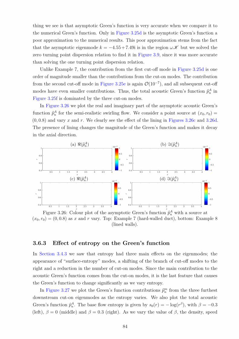
3.26 Colour plot of the asymptotic Green’s function pAn with a source at (x0, r0) =(0, 0.8) as x and r vary. Top: Example 7 (hard-walled duct), bottom: Example8 (lined walls). . . . . . . . . . . . . . . . . . . . . . . . . . . . . . . . . . 84
3.27 Real and imaginary parts of asymptotic and numerical Green’s function asentropy varies for a source at x− x0 = 0.5 and r0 = 0.8. . . . . . . . . . . . 85
3.28 Colour plot of real part of asymptotic Green’s function pAn with a source at(x0, r0) = (0, 0.8) as x and r vary. We vary the entropy and impedance, andthe rest of the parameters are the same as Figure 3.27. . . . . . . . . . . . 86
3.29 Effect of new dispersion relation on asymptotic Green’s functions from thenumerical eigenmode at k = −10.880 + 14.499i. in Example 4. . . . . . . . 91
xii
3.30 Colour plot of the numerical acoustic Green’s function pAω with a source at(r0, θ0) = (0.8, 0) and x−x0 = 0.5 as r and θ vary. The other flow parametersare Ux = 0.5, hard walls, ω = 25 and h = 0.6. . . . . . . . . . . . . . . . . 92
3.31 Plot of maxr∈[h,1] |pAn (r|r0)| for each azimuthal number n for both hard andlined walls (of impedance Zj = 1− 2i) with the other parameters Ux = 0.5,Uθ(r) = 0.1r + 0.1/r, ω = 25, h = 0.6, x− x0 = 0.5 and r0 = 0.8. . . . . . . 92
4.1 Plot of the pressure eigenfunction for a hydrodynamic mode at k = 44.0081.The parameters are Ux(r) = 0.5 + 0.2(r − 1)2, Uθ = 0.2, n = 15, ω = 25 andh = 0.6. . . . . . . . . . . . . . . . . . . . . . . . . . . . . . . . . . . . . . 100
4.2 Right-hand side of critical layer (solid line) showing first five hydrodynamicmodes (crosses). The parameters are Ux = 0.5, Uθ(r) = 0.1r + 0.1/r, ω = 25,n = 15 and h = 0.6. . . . . . . . . . . . . . . . . . . . . . . . . . . . . . . . 105
4.3 Plot of the hydrodynamic modes as we vary entropy for different flow pa-rameters. . . . . . . . . . . . . . . . . . . . . . . . . . . . . . . . . . . . . . 106
4.4 Graph of shear flow Ux(r) (left) and kc(r) (right) for the flows Xl. . . . . . 1084.5 Plot of (k − 44) exp(0.7629m) against m for each of the ten flows Xl to
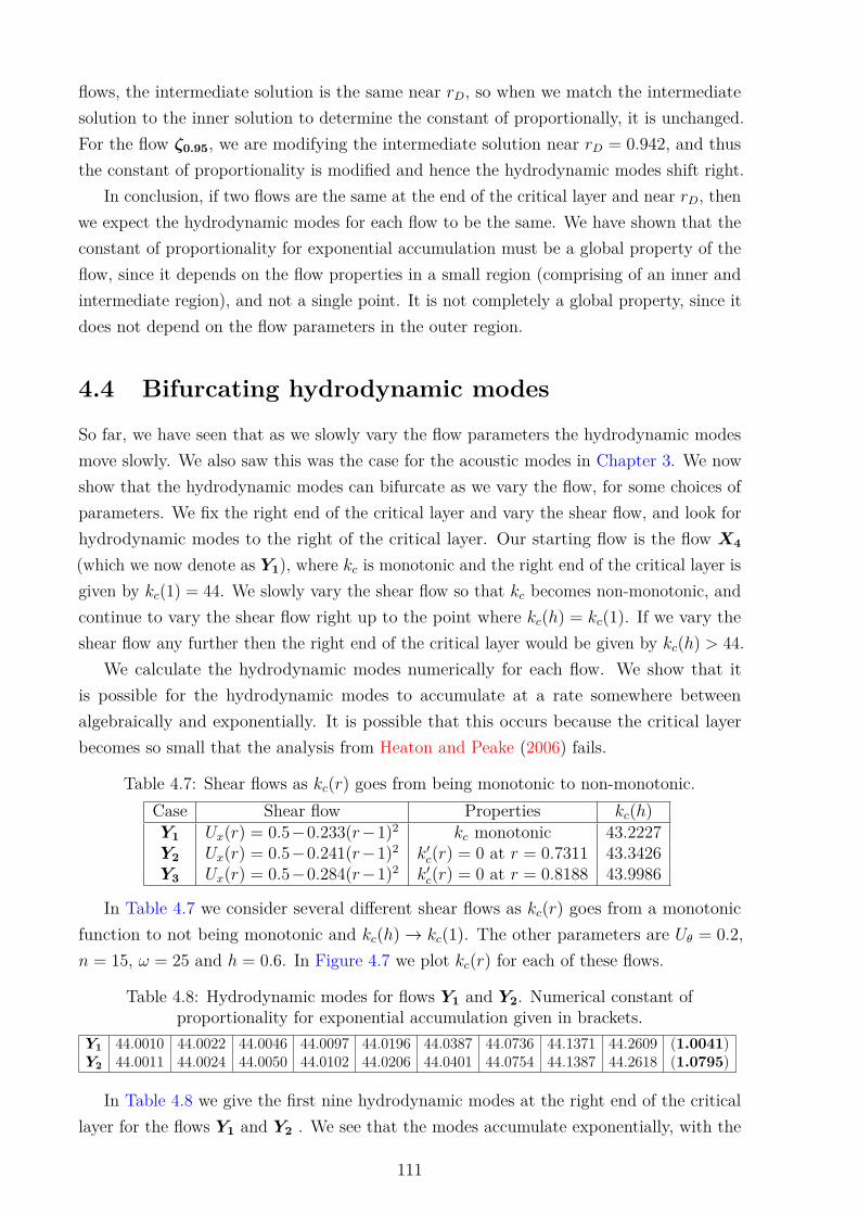
determine constant of proportionality numerically. . . . . . . . . . . . . . . 1094.6 Graph of shear flow Ux(r) (left) and kc(r) (right) for the flows ζa. . . . . . 1104.7 Graph of kc(r) for the flows in Table 4.7. . . . . . . . . . . . . . . . . . . . 1124.8 Plot of hydrodynamic modes as we consider shear flows of the form Ux(r) =
0.5−y(r−1)2, with 0.241 ≤ y ≤ 0.284. The vertical scale is different values ofy in increments of 0.005. The other parameters are n = 15, ω = 25, Uθ = 0.2and h = 0.6. . . . . . . . . . . . . . . . . . . . . . . . . . . . . . . . . . . . 112
4.9 Plot of the pressure eigenfunctions P for the hydrodynamic modes from flowsY1, Y2 and Ya to Yd. . . . . . . . . . . . . . . . . . . . . . . . . . . . . . . 113
5.1 Real and imaginary part of the truncated Fourier series of 1/Zb(θ) whenM = 8 (red) and 1/Zb(θ) (blue). . . . . . . . . . . . . . . . . . . . . . . . . 116
5.2 Plot of truncated Fourier series of 1/Zc(θ) (black) for M = 10 (blue), M = 30(red), M = 100 (green). . . . . . . . . . . . . . . . . . . . . . . . . . . . . . 117
5.3 Plot of regions ωKn as n varies from n = −100 (blue) to n = 100 (red). Weonly plot intervals of n = 10. The other parameters of the flow are ω = 25,h = 0.6, Ux(r) = 0.2 + 0.4r2 and Uθ(r) = 0.1r + 0.2/r. . . . . . . . . . . . . 122
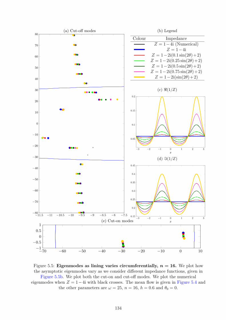
5.4 Plot of shear flow Ux(r) = 0.2 + 0.4r2 and swirl Uθ(r) = 0.1r + 0.2/r. . . . 1335.5 Eigenmodes as lining varies circumferentially, n = 16. . . . . . . . . . . . . 1345.6 Close up of trajectories of eigenmodes from Figure 5.5 as we vary the
impedance function Zς . . . . . . . . . . . . . . . . . . . . . . . . . . . . . . 1355.7 Asymptotic Green’s function for each mode as the impedance function varies
when n = 16 with x− x0 = 0.5 and r0 = 0.8. The other parameters are givenin Figure 5.5. . . . . . . . . . . . . . . . . . . . . . . . . . . . . . . . . . . 136
xiii
5.8 Eigenmodes as lining varies circumferentially, n = −25. . . . . . . . . . . . 1375.9 Close up of trajectories of downstream eigenmodes from Figure 5.8 as we
vary the impedance function Zς . . . . . . . . . . . . . . . . . . . . . . . . . 1385.10 Asymptotic Green’s function for each mode as the impedance function varies
when n = −25 with x − x0 = 0.5 and r0 = 0.8. The other parameters aregiven in Figure 5.5. . . . . . . . . . . . . . . . . . . . . . . . . . . . . . . . 139
6.1 Plot of <(PFs (x, ω)) for a straight and serrated edge at fixed z = −5. The
6.3 Plot of pdiff for serrations Fµ(z) = a sin(µz) as µ and a vary. The parametersare ω = 1, u0 = 0.25, A = (−1, 1,−2), B = (3, 1, 2) and xe = (−3, 0, 1). . . 153
6.4 Plot of <(PFs (x, ω)) for a straight and serrated edge at fixed z = −5. The
6.5 Effect of serrations of the form Fµ(z) = 0.5 sin(µz) on <(PFs (x, ω)). The
parameters are given by ω = 1, u0 = 0.25, A = (1, 2, 1), B = (1, 1, 2) andxe = (0, 0, 0). The colour scale is the same on each plot. . . . . . . . . . . 154
6.6 Plot of pdiff against serration angle ]Fµ for Fµ(z) = 0.5 sin(µz). The eddyparameters are A = (1, 2, 1), B = (1, 1, 2) and xe = (0, 0, 0). The otherparameters are u0 = 0.25 and ω = 1 (blue), ω = 0.2 (red). . . . . . . . . . 154
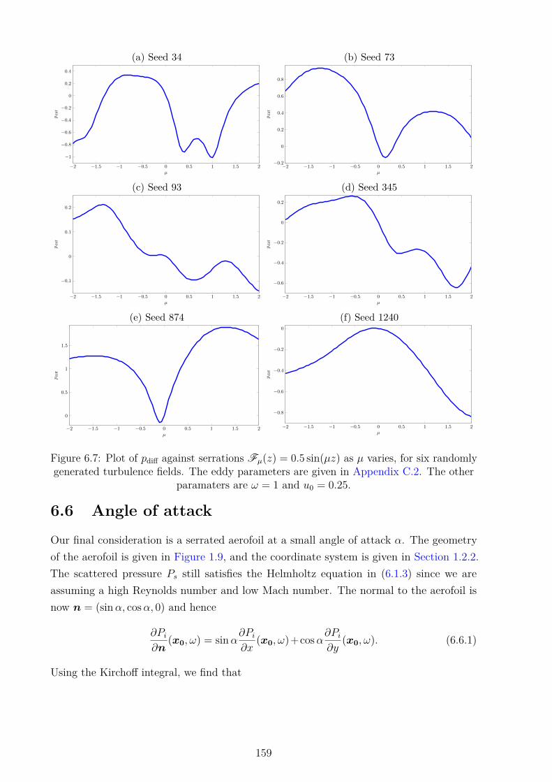
6.7 Plot of pdiff against serrations Fµ(z) = 0.5 sin(µz) as µ varies, for six randomlygenerated turbulence fields. The eddy parameters are given in Appendix C.2.The other paramaters are ω = 1 and u0 = 0.25. . . . . . . . . . . . . . . . 159
6.8 Plot of <(PF ,αs (x, ω)) for a straight edge and serrated edge at angle of attack
α = 6° and θ? = π + α. The parameters are ω = 0.5, u0 = 0.25 with eddyA = (1, 1, 1), B = (1, 1, 1) and xe = (−1,−0.1, 0). . . . . . . . . . . . . . 162
6.9 Plot of pdiff for serrations Fµ(z) = 0.5 sin(µz) as µ varies, for aerofoils atdifferent angle of attacks. The parameters are ω = 0.5, u0 = 0.25 with eddyA = (1, 2, 1), B = (1, 1, 2) and xe = (−1, 0.1, 0). . . . . . . . . . . . . . . . 163
A.1 Plot of a chebfun of the Airy function Ai(x). . . . . . . . . . . . . . . . . . 178A.2 Plot of a chebfun of the Airy function Ai′(x). . . . . . . . . . . . . . . . . . 179A.3 Plot of Chebfun solution g(x) of the differential equation 0.1g′′(x)+g′(x) =−1
with boundary conditions g(−5) = 0 and g(5) = 0. . . . . . . . . . . . . . 179A.4 Chebfun eigenvalues for the eigenvalue problem (A.2.2) with associated
4.1 Analytic accumulation rate λ∗(1) and numerical constant of proportionalityof the hydrodynamic modes for the flows given in Figure 4.2. . . . . . . . . 106
4.2 Different shear flows with Ux(1) = 0.5 and U ′x(1) = 0. . . . . . . . . . . . . 1074.3 More shear flows with Ux(1) = 0.5 and U ′x(1) = 0. . . . . . . . . . . . . . . 1084.4 First nine hydrodynamic modes for the flows Xl. . . . . . . . . . . . . . . 1084.5 Constant of proportionally for each of the ten flows Xl. . . . . . . . . . . . 1094.6 First five hydrodynamics modes for the flows ζa. . . . . . . . . . . . . . . . 1104.7 Shear flows as kc(r) goes from being monotonic to non-monotonic. . . . . . 1114.8 Hydrodynamic modes for flows Y1 and Y2. Numerical constant of propor-
tionality for exponential accumulation given in brackets. . . . . . . . . . . 111
Aj, Bj Constants in solution vj after using WKB method
B Gaussian strengths of eddy Φ
Bj∞ Infinite vector of constants we solve for in asymptotic eigenmode problem
when lining varies circumferentially
Bj = (Bjm) Finite vector of constants we solve for in asymptotic eigenmode problem
when lining varies circumferentially
B Function in differential equation for unsteady potential ϕ
BR Number of rotor blades
C Amplitudes of eddy Ψ
c Total speed of sound of the flow
c0 Base flow speed of sound
cm, dm Fourier series coefficients of 1/Z(θ)
cp, cv Specific heat capacities at constant pressure and volume respectively
D Gaussian strengths of eddy Ψ
D Function in differential equation for unsteady potential ϕ
D0/Dt Base flow convective derivative
de Displacement between source positions of two eddies
ej Unit vector in j-th direction
e Internal energy per unit mass of total flow
fj Function used in boundary condition for vj
xvii
fS(t) The rotor-stator space Sf is defined by fS(x, t) = 0
G Green’s function
GF Green’s function for serrated half plane defined by x > F (z)
[GF ] Jump in Green’s function GF over serrated aerofoil
mGF The m-th component in the series of GF
Gn Axial Fourier transform of the n-th azimuthal Fourier series coefficient ofGω
GCLn Contribution to Gn from the integral enclosing the critical layer and
hydrodynamic modes
Gω Reduced Green’s function at a particular frequency in the duct
g1, g2 Solutions to the homogeneous equation that Gn solves with certain bound-ary conditions
H Heaviside function
H A smooth but non-analytic approximation of the Heaviside function
H(1)νm , H(2)
νm Hankel functions of the first and second kind, order νm
h Non-dimensionalised inner radius of the duct
Iα,lγ , Jαγ Integrals needed to calculated the scatted pressure Ps for an aerofoil atnon-zero angle of attack
i Imaginary unit
J Jump in first order derivative when finding the Green’s function Gn
Jνm Bessel function of the first kind, order νm
j Used for indexing, j ∈ 1, 2, j ∈ h, 1, j ∈ 1, 2, 3 or j ∈ x, y, z
K Isentropic bulk modulus of a fluid
Kl Modified Bessel function of the second kind, of order l
k Axial wavenumber and eigenmode
kA, kB, kC Specific hydrodynamic eigenmodes
kc(r) Function that defines the critical layer
xviii
kmn A specific acoustic eigenmode indexed by m at a specific azimuthal numbern
k±m A specific hydrodynamic eigenmode indexed by m (at a particular az-imuthal number)
l Used for indexing
M Number of terms taken in truncated Fourier series of 1/Z(θ)
M(r) Mach number of flow
m Used for indexing, generally m ∈ Z or m ∈ N
N , N1 Number of non-zero terms in finite eigenmode system when lining variescircumferentially, with N1 = 2N + 1
Ne Number of eddies
n Unit normal
n Azimuthal number
P Fourier transform of pressure perturbation
PI , PO Inner and outer solutions for the pressure P
Pi Fourier transform of incident pressure
∆Pl Pressure jump over the l-th blade of the rotor
Ps, PFs , PF ,α
s Fourier transform of scattered pressure for an aerofoil with serration F atangle of attack α
P Used in numerical eigenvalue problem, P = kP
p Total pressure of the flow
p Pressure perturbation
p Pressure perturbation multiplied by H(fS)
p0 Base flow pressure
pdiff Proxy for measuring noise reduction for serrated aerofoils, pdiff = log(PF/P0)
p†diff Actual noise reduction in Decibels for serrated aerofoils
pi Incident pressure
xix
pn Axial Fourier transform of the n-th azimuthal Fourier series coefficient ofpω
pAn Contribution towards pn from all the acoustic modes
pCLn Contribution to pn from the integral enclosing the critical layer and hy-drodynamic modes
pmn Contribution to pn from the acoustic eigenmode kmn
ps Scattered pressure
pω Reduced Green’s function at a particular frequency to match Posson andPeake (2013b)
pAω Contribution towards pω from all the acoustic modes
Q1 Term in integrand to calculate the scattered pressure Ps for a single eddy
Qα1 Term in integrand to calculate the scattered pressure Ps for a single eddy
at angle of attack α
QS2 , QD
2 Term in integrand to calculate the scattered pressure Ps for two eddies,with the same or different sources
QDNe Term in integrand to calculate the scattered pressure Ps for Ne eddies,
with different sources
qn Function in WKB differential equation. The number of zeros of qn deter-mines the form of the solution
R Ideal gas constant, R = cp − cv
R(r) Fourier transform of density
Re Eddy radius, dependent on source position xe of the eddy
r Non-dimensionalised radial coordinate
r = (r?, θ?, z?) Modified cylindrical coordinates in x-y plane, centred at (F (z), 0)
r0 = (r?0, θ?0, z?0) Source position in modified cylindrical coordinates
rc (rcn) Zero of qn
rc,j Zeros of qn when we have multiple zeros
rcl Zero of Ω
r∗cl Critical point of kc, k′c(r∗cl) = 0
xx
rD Zero of D
S Fourier transform of entropy perturbation
s Total entropy of the flow
s Entropy perturbation
s0 Base flow entropy
s± (s±n ) Function used to find K , K = s+(R) ∪ s−(R)
T Temperature of total flow
Tjl Lighthill stress tensor
t Time
U, V,W Fourier transform of velocity perturbations
Uθ(r) Swirl profile for base flow
Ux(r) Shear profile for base flow
(u, v, w) Total velocities of the flow (in x, r and θ directions respectively)
(u, v, w) Velocity perturbations
(u, v, w) Velocity perturbations multiplied by H(fS)
(u0, v0, w0) Base flow velocities
v1, v2 Scaled versions of g1 and g2 used in WKB solution
vS Surface speed of rotor-stator space Sf
Xl, Yl Base flow regimes when calculating hydrodynamic modes
x Non-dimensionalised axial coordinate
x = (x, r, θ) Cylindrical coordinates in the duct
x0 = (x0, r0, θ0) Source position in the duct
xe Source position of the eddy, xe = (xe, ye, ze)
Zp Non-isentropic factor, Zp = p/c20 − ρ
Zj (Z) Complex impedance of acoustic lining at duct walls
Za, Zb, Zc, Zς Complex impedances of acoustic lining at duct walls which varies circum-ferentially
xxi
zs Centre of modified cylindrical coordinates, zs = (F (z0), 0, z0), so that|x− zs|2 = r?2 + (z − z0)
z Non-dimensionalised height above aerofoil
Greek Characters
α Angle of attack of aerofoil
β Varying parameter in base flow entropy s0(r) = − log(rβ)
βjl Product of amplitudes and Gaussian strengths in j and l direction, for asingle eddy βjl = AjBjAlBl
Γ Contour for calculating the inverse Fourier transform of the Green’s func-tion, using the Briggs-Bers method
ΓCLH Contour enclosing the critical layer and hydrodynamic modes
γ Ratio of specific heat capacities
γ(kz) Function used in Green’s function for serrated aerofoil, γ(kz) =√ω2 − k2
z
γjl Sum of Gaussian strengths in j and l direction, for a single eddy γjl =Bj +Bl
δ(f) Dirac delta
δjl Kronecker delta
ε Small parameter
εr Similar to Levi-Civita symbol, εh = 1 and ε1 = −1
ζ Compressibility factor, used in the numerical eigenvalue problem
ζl Base flow regime when calculating hydrodynamic modes
η Scaled azimuthal number, η = n/ω
θ Circumferential coordinate
ι (ι?) Angle between r (r?) and z − z0, used to calculate Green’s function of aserrated aerofoil in the far field
κ Scaled axial wavenumber, κ = k/ω
κmn A specific scaled acoustic eigenmode indexed by m at a specific azimuthalnumber n
xxii
Λj Finite matrix in asymptotic eigenmode problem when lining varies circum-ferentially
Λj∞ Infinite matrix in asymptotic eigenmode problem when lining varies cir-
cumferentially
λ, λ∗ Defines accumulation rate for hydrodynamic modes, λ∗ is same as λ butwith additional entropy factor related to E
µ Free parameter, different in each chapter
µj Finite vector in asymptotic eigenmode problem when lining varies circum-ferentially
µj∞ Infinite vector in asymptotic eigenmode problem when lining varies cir-cumferentially
ν (ν∗) Related to λ (λ∗) with 2λ =√
4ν − 1 (2λ∗ =√
4ν∗ − 1)
νm νm = m/2
ρ Density of the total flow
ρ Density perturbation
ρ Density perturbation multiplied by H(fS)
ρ0 Base flow density
Σh, Σ1 Functions relating to the impedance at the duct walls
σh, σ1 Functions relating to the impedance at the duct walls, zero for hard walls
ς Free parameter, different in each chapter
τ , τ (τn, τn) Variables that the Airy functions act on in the WKB solution
τjl Viscous stress tensor
Υ (Υn) Function in differential equation for Gn
Υ∗ (Υ∗n) Scaled version of Υ, Υ = ωΥ∗
Φ, Ψ Eddies
Φ (Φn) Scaled version of Ω, Ω = ωΦ
Φj,l Shape function of the l-th eddy, with either a Gaussian or Mexican hatprofile
ϕ Unsteady potential
xxiii
φ Fourier transform of unsteady potential ϕ
χ Function relating to the Fourier transform of unsteady potential, φ
χI , χO Inner and outer solutions of χ
Ψn Integral of √qn between rc and 1, used in WKB method for one turningpoint solution
Ψjn Extension of Ψn when we have two zeros of qn
ψn Integral of √qn in the duct, used in WKB method for zero turning pointsolution
Ω (Ωn) Function in differential equation for Gn, Ω = 0 defines critical layer
Ω, (Ωn) Related function to Ω, used in the numerical eigenvalue problem
ΩR Angular speed of the rotor
ω Non-dimensionalised frequency
Other Characters
A Coefficient of highest derivative in differential equation for pressure P
Am Coefficient of constant Am in vm(r)
Am Coefficient of constant Am in v′m(r)
B, B Coefficient of first order derivative in differential equation for pressure P ,B = B/A
Bm Coefficient of constant Bm in vm(r)
Bm Coefficient of constant Bm in v′m(r)
C, C Coefficient in differential equation for pressure, P , C = C/A
D, Dmass, De Surface source terms from momentum, mass and energy equations
E(r) Extra entropy term in ν∗ for accumulation rate of hydrodynamic modes
E, EAOA Exponential terms needed to calculate the scattered pressure Ps, EAOA
reduces to E at zero angle of attack
FPP , FM Sixth order differential operators acting on pressure perturbation p inacoustic analogy
F Serration function for leading edge of aerofoil
xxiv
]F Angle of serration F at z = 0
H Function in volume source terms in acoustic analogy
K+n Set of all acoustic downstream eigenmodes for a specific azimuthal number
n
K−n Set of all acoustic upstream eigenmodes for a specific azimuthal number n
KCL Critical layer
K (Kn) Region of κ space when we should use the one turning point solution inthe WKB method
PF , PF ,α Power of scattered pressure for an aerofoil with serration F at angle ofattack α
Q If Q > 0 then <(qn) > 0 at r = 1 and <(qn) < 0 at r = h
Qj Extension of Q to when we have two zeros of qn
R, T Differential operators in the acoustic analogy
R Region of r space when we should use the one turning point solution inthe WKB method
Sf (x, t) Space occupied by the rotor and stator in the duct
S, Smass, Se Volume source terms from momentum, mass and energy equations
SM , SMV , SMS Source terms in Mathews’ acoustic analogy
SPP , SPPFWH Source terms in Posson and Peake’s acoustic analogy
U0 Function in differential equation for unsteady potential ϕ, dependent onmean flow
Uθ Function in differential equation for Gn which depends only on swirl Uθ
Uθ Function in acoustic analogy which depends only on swirl Uθ
V (Vn) Wronskian of v1 and v2
W (Wn) Wronskian of g1 and g2
Xn,m, X ∗n,m Coefficients in boundary condition for vn when lining varies circumferen-tially
Zn,m, Z∗n,m Coefficients in boundary condition for gn when lining varies circumferen-tially
xxv
Function spaces
C∞c (R) Space of test functions, which are smooth and have compact support
L1loc(R) Space of locally integrable functions, f ∈ L1
loc(R) if´K|f |dx <∞ for all
compact sets K
Other notation
1K Indicator function for a set K; 1K =
1 x ∈ K
0 x ∈ KC
Bar derivatives Generalised derivatives
Complement The complement of a set K is KC = C\K
Double dagger ‡ Quantities with dimension
Subscript 0 Base flow functions
Tilde Function multiplied by Heaviside function to make generalised function
Underlined Total function, sum of perturbation and base flow
Abbreviations
ACARE Advisory Council for Aeronautics Research in Europe
BPF Blade passing frequency
CAA Computational aeroacoustics
CFD Computational fluid dynamics
EPN Effective perceived noise
SPL Sound pressure level
WKB Wentzel-Kramers-Brillouin method (Bender and Orszag, 1978) for solvinga differential equation with a small parameter
xxvi
Chapter 1
Introduction
1.1 Background
Environmental concerns such as noise pollution, emission of greenhouse gases and fuelefficiency mean that designing a modern aeroengine is a challenge. In 2002 the AdvisoryCouncil for Aeronautics Research in Europe (ACARE) set targets for 2020 such as a 50%cut in carbon dioxide (CO2) emissions, an 80% cut in nitrous oxides (NOx) emissions and a50% reduction of effective perceived noise (EPN) from their 2000 levels (ACARE, 2002).In 2011 the High Level Group on Aviation Research (Flightpath, 2011) proposed strictertargets by 2050, codenamed Flightpath 2050. They aim to achieve a 75% cut in CO2
emissions, a 90% cut in NOx emissions and a 65% reduction of effective perceived noise,all in relation to 2000 levels. According to The Clean Sky Joint Technology Initiative1
(Clean Sky), air transport contributes to 2% of all human CO2 emissions and produces628, 000, 000 tonnes of CO2 a year. In 2008 the UK introduced the Climate Change Act(Climate Change Act, 2008) which contains legally binding targets. However, it does notcover international aviation emissions because of a lack of agreement over allocation offlights.
Despite these environmental concerns, demand for air travel is booming, and theworldwide aircraft fleet is expected to double in 20− 25 years. This growth would requirethe equivalent of 1300 new international airports, leading to additional environmentalconcerns. Passengers will also be expecting better service. Flightpath 2050 also expects90% of travellers on European flights to complete their journey door to door in under fourhours and flights to arrive within one minute of the planned time.
The emission targets have led to a number of European funded collaborative projects,such as Clean Sky and ENOVAL. Clean Sky’s partners include major industrial bodiessuch as Rolls-Royce and Airbus, universities, research institutions and many other small tomedium enterprises. There is limited numerical evidence to show the progress towards the2020 targets. Of the 50% reduction in CO2 emissions, around 15% to 20% was attributedto the aeroengine, and most of the rest to the airframe. The Clean Sky and ENOVAL
projects have generally surpassed the target for the aeroengine, with ENOVAL claiminga 26% reduction on their webpage2. However, the overall target for CO2 emissions lookslikely to be missed, according to Clean Sky (2014), and will instead be around 30% to 40%.Published data suggests that noise reduction will be very close to the target, but probablyfall short. ENOVAL2 suggest that there will be a 9.3dB decrease in EPN, corresponding toa 48% reduction, while Clean Sky (2014) suggest the noise reduction will be between 30%and 50%. It appears that the NOx emission target will be missed by a significant margin,with prediction of around a 20% to 40% reduction by Clean Sky (2014).
(a) General Electric GE36 open-rotorengine.3
(b) Safran open-rotor engine fromClean Sky.4
Figure 1.1: Old and modern open-rotor engine designs.
Figure 1.2:Open-rotor blade.5
One of the main outcomes of these targets is the re-emergence ofopen-rotor engines (or propfans) which usually consist of a number ofcontra-rotating propellers. These were originally popular between the1970s and the 1990s, with designs including the General Electric GE36(Figure 1.1a). The Clean Sky project has seen the development of new,cutting edge open-rotor designs, for example the design from Safranin Figure 1.1b. Many other manufacturers are developing open-rotortechnology and these could be in commercial aircraft before 2030, witha concept from Rolls-Royce shown in Peake and Parry (2012).
Despite being more fuel efficient than the current turbofans, re-search of open-rotor engines was almost universally dropped in the1990s. This was due to major concerns around noise, safety and per-formance whilst plummeting fuel prices meant that the design’s majoradvantage, its efficiency, was becoming less important. At typical cruising speeds the flowaround the rotating open-rotor blades in old designs could become supersonic, causingshocks to form around the blades which significantly reduced performance. However, modernopen-rotor designs use more blades and these blades are highly swept to prevent shocks andhence improve performance. In Figure 1.2 we see a blade from the Safran open-rotor. The
two main concerns that new open-rotor designs need to overcome are related to noise andsafety. The lack of casing around the open-rotor means there is no containment of debris incase of events such as a bird strike. Additionally, the lack of casing compared to a turbofanmeans we have very limited control of the noise. The casing from a turbofan is often fittedwith an acoustic liner to dampen and absorb noise.
In contrast to the open-rotor technologies being developed in Clean Sky, ENOVALis solely focussed on the conventional turbofan. Today, turbofans are used on nearly allmodern commercial aircraft. The major manufacturers of turbofans are General Electric,Rolls-Royce and Pratt & Whitney, and we show a typical, modern turbofan from GeneralElectric in Figure 1.3. The first turbofan to be developed was the Rolls-Royce Conway,around fifty years ago, when Sir Frank Whittle conceived the idea of the by-pass aeroengine6.This technology replaced turbojet engines, which produced all of their thrust from theturbine and were very inefficient.
Fan Stators Combustion chamber
Low-pressurecompressor
High-pressurecompressor
Turbines
Figure 1.3: Schematic of a modern General Electric GEnx-1B turbofan.7
The turbofan is designed so that incoming air is split into two channels, as seen in theschematic in Figure 1.3. Some of the air enters the compressor, turbine and combuster,which provides most of the thrust. The rest bypasses the turbine, but is still sped up bythe fan, so it provides additional thrust. The mixing of the hot core flow of air comingout of the nozzle and the cooler bypass flow of air creates what is called jet noise. Theratio between these flows of air is called the bypass ratio. A higher bypass ratio means thatmore of the air bypasses the turbine and core of the aeroengine. Since the early turbofans,manufacturers have been increasing the bypass ratio, which has led to changes in the overallnoise from the turbofan, although many other factors are also responsible. Figure 1.4 showshow the different components of the turbofan contribute to the noise from a modern designand an early turbofan.
Figure 1.4: Effective perceived noise from early and modern turbofans, taken from Peakeand Parry (2012).
We see that the jet noise has significantly decreased and the fan noise is now thedominant source for modern turbofans. The ENOVAL project is looking to reduce noise byfurther increasing the bypass ratio and using a number of new developments to the turbofanincluding new blade technologies, lightweight casing, new acoustic lining technologies and ashorter design8.
We split the noise into tonal and broadband components. The frequency spectrum for anoise source is a plot of sound pressure level (SPL), measured in Decibels, versus frequency,measured in Hertz. Broadband noise has a frequency spectrum where the amplitude isinsensitive to frequency and there are no dominant frequencies. We see an example ofbroadband noise in Figure 1.5a. Tonal noise is where there are dominant discrete frequenciesin a spectrum. In Figures 1.5b and 1.5c there is tonal noise at 1000 Hz and integer multiplesof it. Tonal noise can be pure, where the SPL is close to zero away from the tones, andwe give an an example in Figure 1.5b. However, most tonal noise sources in an aeroenginehave underlying broadband noise, so away from the tones the SPL is non-zero, and we givean example in Figure 1.5c.
0 1000 2000 30000
20
40
60
Frequency (Hz)
SPL(dB)
(a) Broadband noise.
0 1000 2000 30000
20
40
60
Frequency (Hz)
SPL(dB)
(b) Pure tonal noise.
0 1000 2000 30000
20
40
60
Frequency (Hz)
SPL(dB)
(c) Tonal noise.Figure 1.5: Frequency spectrum for tonal and broadband noise.
For a turbofan, the main sources of fan noise identified by Peake and Parry (2012) are therotor (or fan) self-noise, rotor-stator (or fan-vane) interaction, rotor casing boundary-layerinteraction and droop-fan interaction. In addition, there are sources unique to open-rotors,with the latter two sources for turbofans not present. For a complete overview of all sourcesof noise from an aircraft, see Smith (2004).
Rotor self-noise has both tonal and broadband components. It occurs because of theforces exerted on the fluid (air) from the rotating blades. A subsonic rotor with BR bladesproduces tonal noise at harmonics of the blade passing frequency (BPF). The BPF is BRΩR,where ΩR is the angular speed of the rotor. The tip blade speed can become supersonic,for example at take-off. This causes shocks in the flow around the rotor blade, which thenproduces tonal noise at non-integer multiples of the BPF due to blade-to-blade differencesbetween the shocks. This is generally referred to as multiple pure tone noise or “buzz saw”noise. However, this is largely controlled through the use of acoustic liners and changing thegeometry of the rotor blades. We show the comparison between the subsonic and supersonicfrequency spectra in Figure 1.6. We also see that the underlying broadband component ofrotor self-noise is significant.
0 1 2 3
30
40
50
60
Frequency (BPF)
SPL(dB)
(a) Noise at subsonic speed.
0 1 2 3
30
40
50
60
Frequency (BPF)
SPL(dB)
(b) Noise at supersonic speed.Figure 1.6: Rotor self-noise at subsonic and supersonic blade speeds.
Rotor-stator interaction noise also has both broadband and tonal elements, and is thedominant broadband and tonal source of noise. The purpose of the stators (or outlet guidevanes) is to straighten the swirling flow, but they do so at the expense of creating noise. InFigure 1.3 we see there are usually a number of stators, with each stator generally havingmore blades than the rotor. The rotor wake is the sum of a uniform rotating flow plus aturbulent wake from each rotor blade, with a typical wake evolution shown in Cooper andPeake (2005, Figure 2). The turbulent wake from the rotor then interacts with the statorsthat block the wake, producing broadband noise. There is also tonal noise produced atharmonics of the BPF. The rotor-stator interaction can be controlled by using the theoryof Tyler and Sofrin (1962). By tuning the turbofan with different combinations of rotorand stator blades we can control the tonal noise (Rienstra and Hirschberg, 2003). In anopen-rotor there is a similar effect due to the wake of the first rotor interacting with thecontra-rotating second rotor (rotor-rotor interaction), and the interaction is louder thanthe rotor-stator interaction due to the increased speed difference.
The rotor casing boundary-layer interaction is a broadband source of noise, and arisesbecause there is only a very small clearance between the casing and the tips of the rotorblades. The presence of a turbulent boundary layer at the casing outer wall produces thenoise, but a careful design of the casing all but alleviates this noise source (Peake and Parry,2012). A final source of tonal noise for turbofans is droop-fan interaction (Peake and Parry,2012). Geometric considerations such as ground clearance dictate that in some designs,the engine intake is not axisymmetric and is squashed at the top or bottom. This lack of
5
symmetry causes the tonal noise.In an open-rotor there are new sources to deal with in addition to rotor self-noise and
rotor-rotor interaction. The main new source is due to installation effects from the lack ofengine casing. Broadband noise is produced from the rotor wake interacting with the wings,fuselage or pylons (structural supports such as in Figure 1.1b). New technologies such astrailing-edge blowing reduce pylon noise. The graph in Peake and Parry (2012, Section7.2) shows that with blowing technology implemented, the pylon effects are minimal. Inaddition to rotor-rotor interaction there is a similar source of tip-vortex-interaction whichis described in Peake and Parry (2012).
Next, we consider how to mathematically model a turbofan aeroengine, such as the Rolls-Royce Trent 700 in Figure 1.7a. Figure 1.7b shows a model of a Rolls-Royce Trent 1000that can be used in computational fluid dynamics (CFD) to model the airflow through theaeroengine.
Our aeroengine model is considerably simpler, and is an infinite duct, with the airflowing between two cylinders. This is a suitable approximation for considering rotorself-interaction and rotor-stator interaction. In Figure 1.8a we see the cylindrical coordinatesystem, with x the axial coordinate, r the radial coordinate and θ the azimuthal coordinate.
We let u, v, and w be the velocities in the x, r and θ directions respectively. We referto the velocity in the x direction, u, as the shear, and the velocity in the θ direction, w, asthe swirl. We split the inviscid total flow (underlined) of air into a base flow (subscript 0)
where u = (u, v, w) is the total velocity of the air, ρ is the total density and p the totalpressure.
Non-dimensionalisation
We use ‡ to denote quantities with dimension. Let the inner and outer duct walls be givenby r‡ = h‡ and r‡ = d‡ respectively. We non-dimensionalise all distances by d‡, so that theinner wall lies at r = h := h‡/d‡ and the outer wall at r = 1. We non-dimensionalise allvelocities by the speed of sound at r = 1, c‡0(1). Finally, we non-dimensionalise times byd‡/c‡0(1). Thus we have
r = r‡
d‡, x = x‡
d‡, u = u‡
c‡0(1), u0 = u‡0
c‡0(1), t = t‡c‡0(1)
d‡, ω = ω‡d‡
c‡0(1), (1.2.2)
where ω is the frequency. We could also non-dimensionalise the pressures and densities byp‡0(1) and ρ‡0(1).
Rotor and stator in the duct
To model the rotor blades and the stator we can use simple cascade models such as fromPosson et al. (2009). We show a simple geometric model in Figure 1.8b, where we haveunwrapped the θ coordinate. The rotor is rotating at an angular speed of ΩR, while thestator blades are fixed. We consider the blades to be infinitely thin planes, with zero leanor sweep. The blade stagger angle (angle between the blade and x axis) is positive for the
7
rotor and negative for the stator, which allows the stator to straighten the swirling flowfrom the rotor.
Acoustic lining in the aeroengine
In the duct, we either consider the walls to be hard or have an acoustic lining. If we considera duct with hard walls then the boundary condition for the flow is very simple and becomesthe no-penetration boundary condition. Thus, the normal velocity must be zero at thewalls, or
v0(h) = v0(1) = v(h) = v(1) = 0, (1.2.3)
with the conditions on v0 coming from the inviscid nature of the flow. Now suppose theduct walls are treated with an acoustic lining to absorb some of the sound energy. Tomathematically model the acoustic lining we introduce the impedances Zh, Z1 ∈ C of theliner at the duct walls. We non-dimensionalise the impedances by Zj = Z‡j c
‡0(1)/p‡0(1). We
further assume that the lining is locally reacting, so these impedances are functions offrequency only, and in fact we assume that these impedances are constant. The real part ofthe impedance corresponds to damping and the imaginary part to reactance. The boundaryconditions for the unsteady flow are the standard Ingard-Myers boundary conditions((Ingard, 1959), (Myers, 1980)), which due to the geometry of the duct are given by
iωv =(−iω + u0
∂
∂x+ v0
∂
∂r+ w0
r
∂
∂θ
)(p
Zh
)on r = h,
−iωv =(−iω + u0
∂
∂x+ v0
∂
∂r+ w0
r
∂
∂θ
)(p
Z1
)on r = 1.
(1.2.4)
In the Ingard-Myers boundary condition we assume the time dependence of the flow is ofthe form exp(−iωt). The impedances we choose are of the form Zj = 1−Zimagi, where Zimag
is positive, as suggested in Posson and Peake (2013a). A typical choice we use is Zj = 1− 2i.We always take the imaginary part of the impedance negative because of how we later defineour Fourier transforms, so that the lining absorbs energy. We consider <(Zj) = 1 a realisticvalue (Posson and Peake, 2013a) of impedance after non-dimensionalisation. The case ofhard walls corresponds to an impedance of Zj =∞, for which the boundary conditions in(1.2.4) reduce to (1.2.3).
When using the Ingard-Myers boundary conditions we can (and will) consider a baseflow which does not satisfy the no-penetration boundary condition (v0 = 0) or the no-slipboundary conditions (u0 = w0 = 0). This is because in the derivation of the Ingard-Myersboundary conditions a boundary layer is added to the base flow so that both the no-slipand no-penetration boundary conditions are satisfied.
8
1.2.2 Modelling stators as aerofoils
To investigate the effect of turbulence hitting a stator, we model a single aerofoil bladeas an infinitely thin half plane. To study the effect of serrations we consider a serrationfunction F (z) (such as a sinusoidal wave or sawtooth) on the leading edge of the aerofoil.We see this in Figure 1.9. Mathematically, the aerofoil is defined by
(x, y, z) ∈ R3| z ∈ R, F (z) cosα < x <∞, y = x tanα, (1.2.5)
where α is the angle of attack of the aerofoil. We introduce serrated cylindrical coordinates
x
z
y
(a) Sinusoidal serrated aerofoil.
x
z
y
α
(b) Sawtooth serrated aerofoil atangle of attack α.
Figure 1.9: Geometry of serrated aerofoils.
of (r?, θ?, z?), defined by
(x, y, z) = (cosαF (z?)− r? cos θ?,− sinαF (z?)− r? sin θ?, z?). (1.2.6)
In these modified cylindrical coordinates r? is the distance to the leading edge of the aerofoil,θ? is the angle in the x-y plane, and z? the height. We define θ? such that the two sides ofthe aerofoil correspond to θ? = ±π + α.
When there is no angle of attack we calculate that
(x, y, z) = (F (z?)− r? cos θ?,−r? sin θ?, z?), (1.2.7)
and hence the new coordinates are just cylindrical coordinates in the x-y plane, centred at(F (z?), 0). When we consider the flow around the aerofoil, the flow in the x direction isthe shear u and the flow in the y direction is the swirl w.
9
Non-dimensionalisation
We non-dimensionalise all velocities by the (assumed constant) speed of sound c‡0, so thenon-dimensionalised speed of sound is given by c0 = 1. Since we want to vary the amplitudeand wavelength of serrations, and also the distance parameters in the eddy, we are not ableto use any of these to non-dimensionalise distances by. Instead, we use the frequency to geta quantity d‡, where
ω = ω‡d‡
c‡0. (1.2.8)
We then use d‡ to non-dimensionalise all distances.
1.3 Literature review
The main topic of this thesis is investigating rotor-stator interaction. We do this in twodistinct ways. First, we calculate the Green’s function for pressure in a turbofan duct withswirling mean flow. Second, we investigate the effect of turbulence hitting an isolated statorblade in Chapter 6.
The Green’s function does not directly give us the noise from rotor-stator interaction.There are two possible ways of using the Green’s function we derive in the thesis. Thefirst is to use an acoustic analogy, which is derived in Chapter 2. On the left-hand side ofthe acoustic analogy is a differential operator acting on pressure, and we find the Green’sfunction of this operator. The right-hand side of the acoustic analogy gives us the sourceterms from a rotor and stator. These source terms can be calculated analytically if weassume a very simple geometry of the rotor and stator (such as in Figure 1.8b), as detailedin Posson and Peake (2013b). Once we calculate the sound source terms, we can calculatethe pressure and hence the noise analytically by calculating the convolution of the sourceterms and Green’s function.
Alternatively, the Green’s function can be used in beamforming to analyse noise sourcesin the aeroengine. This has applications to both rotor-stator interaction and rotor self-interaction. Significant recent progress has been made, such as by Sijtsma (2006), andbeamforming is now one of the major processing tools used to analyse microphone array datain aeroengine noise tests. However, until now the Green’s function used in the techniquehas been relatively simple so far, with the most complicated Green’s function only assumingradial, piecewise constant shear flow in the duct (Sijtsma, 2012). In realistic industrialproblems, we need to consider swirling flow, and not using an appropriate Green’s functioncan lead to spurious and inaccurate results from beamforming.
In Chapter 6 we directly compute the pressure (and hence noise) from turbulence hittingan isolated stator blade. This enables us to see the effect of serrations on a single blade,and we show that it is always possible to reduce the noise by choosing a serrated aerofoil,but the optimum choice depends on the turbulence. Although we only consider a veryidealised blade such as those in Figure 1.9, we could use cascade models such as those in
10
Posson et al. (2009) to calculate the effect of turbulence hitting a whole stator instead of asingle blade. Also, we could apply the results of Chapter 6 to other aerofoils, such as theaircraft wings to understand and reduce the noise from the airframe.
Chapter 2
Lighthill (1952) famously derived the first acoustic analogy by rearranging the Navier–Stokesequations into a single equation for the density perturbation ρ. The analogy was derivedfor a medium at rest, with the left-hand side the wave operator acting on the densityperturbation and the right-hand side the other terms such as pressure and velocity. Theexact rearrangement is given by
∂2ρ
∂t2− c2
0∆ρ = ∂2Tjl∂xj∂xl
, (1.3.1)
whereTjl = ρujul + (p− c2
0ρ)δjl − τjl, (1.3.2)
with τjl the viscous stress tensor, δjl the Kronecker delta and c0 the speed of sound of thebase flow. The right-hand side is commonly referred to as the (double) divergence of theLighthill stress tensor Tjl and is interpreted as a sound source. For this analogy, the freespace Green’s function of the wave operator is easily found (see for example Duffy (2001))and approximations exist to calculate the source terms on the right-hand side such as thosein Colonius and Lele (2004).
Lighthill’s analogy has been extended in a number of ways. These include consideringmoving surfaces in the flow, considering moving media and looking at different variables onthe left-hand side.
Curle (1955) and Ffowcs Williams and Hawkings (1969) addressed this first extension.Curle considered solid static surfaces, while Ffowcs Williams and Hawkings generalisedthis further to account for arbitrary, moving impermeable or permeable surfaces. Theapproach by Ffowcs Williams and Hawkings (1969) uses the theory of what is now knownas generalised functions (see Section 1.4.1), which allows clear identification of the sourceterms as monopole, dipole or quadrupole sources.
By considering non-zero base flows, we can extend the acoustic analogy to moving media.Lilley (1974) extended Lighthill’s analogy to account for shear flow. On the left-hand sideof Lilley’s analogy is a third order, non-linear operator acting on the logarithm of thepressure. This non-linear operator is often approximated by the linear Pridmore-Brownoperator (Goldstein, 2001), although this makes the source terms on the right-hand sidevery complicated. Additionally, Goldstein showed that for small fluctuations we can replacethe logarithm of pressure by just pressure. The exact source terms on the right-hand sideof Lilley’s analogy with the Pridmore-Brown operator are given in Colonius et al. (1997),which also gives a simpler approximate form of the source terms, based on the work in
11
Goldstein (1984).Other extensions consider the acoustic analogy acting on different variables. For example,
Goldstein (2001) considered the variable (p/p0)(1/γ) − 1, where γ = 1.4 for air. Morfey andWright (2007) also considered several different pressure related variables. Each differentformulation of their analogy is suited to a particular type of flow, for example the acousticanalogy acting on the pressure related variable from Morfey and Wright (2007) is usefulwhen the flow is being heated. The analogy by Morfey and Wright also deals with movingsurfaces and a moving medium.
In Posson and Peake (2013b) an acoustic analogy is developed with a moving medium(with shear and swirl) and moving surfaces in an infinite duct. The acoustic analogy is asixth order linear operator acting on the pressure perturbation, which is obtained fromrearranging the Euler equations. In their own words, they define it as a “generalisation ofFfowcs Williams-Hawkings’s acoustic analogy to swirling mean flow with duct walls”.
In Chapter 2 we extend the acoustic analogy from Posson and Peake (2013b) to a swirling,non-isentropic base flow, so the base flow entropy varies. This necessitates including theenergy equation in the derivation of the acoustic analogy.
Chapter 3
In Chapter 3 we find the Green’s function for the acoustic analogy derived in Chapter 2.We do this both numerically and analytically using high-frequency asymptotics and theWKB method (see Appendix A.1). Our main interest is the analytic Green’s function,which we compare to numerical results. The Green’s function we calculate applies for flowwith arbitrary shear and swirl in a lined, infinite duct. The method we use to calculate theGreen’s function requires us to first calculate the eigenmodes of the flow (see Section 1.4.3),which we do by finding an asymptotic dispersion relation which these eigenmodes satisfy.
There are two compelling reasons for calculating the Green’s function analytically. First,it allows us to better understand the behaviour of the Green’s function by writing it in termsof elementary functions. Second, the asymptotic method offers us some speed advantagescompared to computing the numerical Green function. However, both of these advantagesare tarnished somewhat by the fact that we have to currently solve the asymptotic dispersionrelation for the eigenmodes numerically, and often need to use the numerical eigenmodes asa starting guess to find the asymptotic eigenmodes.
When calculating the Green’s function from the acoustic analogy we should choose aGreen’s function tailored for the geometry. For example, for flow in a duct, cylinder orbetween two walls our Green’s function should have appropriate no-penetration and no-slipboundary conditions. Wundrow and Khavaran (2004) consider a high-frequency, free-fieldasymptotic Green’s function in the case of no swirl, but since the Green’s function is nottailored to the duct, it is not very relevant. In Cooper and Peake (2005) and Heaton andPeake (2005) the eigenmodes and eigenfunctions for swirling flow in a hard-walled infiniteduct were calculated asymptotically, using the WKB method. In both papers they show we
12
can get turning points in the WKB method, corresponding physically to caustics (Cooperand Peake, 2005, Figure 10). Heaton and Peake (2005) use the uniformly-valid Langersolution for the eigenfunctions, which we will also use.
In Vilenski and Rienstra (2007a,b) a lined infinite duct is considered, but for noswirl. They only seek the eigenmodes and eigenfunctions of the resulting Pridmore–Brown(Pridmore-Brown, 1958) differential equation, and not the Green’s function. They comparenumerical and asymptotic results for only a couple of simple cases, and do not elaborate toomuch on their actual method for calculating the asymptotic eigenmodes. Instead, they focuson the trajectories of the asymptotic eigenmodes as they vary the impedance of the lining.In Posson and Peake (2012) and Posson and Peake (2013b) the sixth order acoustic analogywas derived and the eigenmodes and Green’s functions were calculated numerically. A baseflow with swirl flow and constant entropy was considered in a hard-walled infinite duct. InPosson and Peake (2013a) the results were extended to an infinite duct with acoustic lining.
There has also been research into the correct boundary conditions to use in a lined duct.Although the Ingard-Myers boundary conditions are often used, recent work by Brambley(2011) and Khamis and Brambley (2016) showed the Ingard-Myers boundary condition isnot well-posed and does not always model the physics correctly, leading to an inaccurateboundary condition. However, the new proposed boundary condition involves integral termsand is harder to work with, so we only consider the Ingard-Myers boundary condition.
We also consider the Green’s function in the case of variable entropy, which requiresthe new acoustic analogy from Chapter 2. Relatively little work has been carried out onthe effect of entropy on the eigenmodes and Green’s function, although Tam and Auriault(1998) considered it. They calculate eigenmodes and a Green’s function in the case of simpleswirling flow in an infinite hard-walled duct, and their choice of base flow density ensuredthe entropy of the base flow varied. We instead specify the base flow entropy, and calculatethe density from this, which is the method used in Cooper (2006). We use the base flowentropy from Cooper (2006), although it is easy to consider different forms.
Chapter 4
In Chapter 3 we calculate the eigenmodes of the flow, but we are unable to calculate someof them (the hydrodynamic modes - see Section 1.4.3) using our high-frequency asymptotics.In Chapter 4 we predict the hydrodynamic modes asymptotically by using a differentmethod. We numerically calculate these modes for a variety of different base flows, some ofwhich have varying entropy, and compare to the asymptotic results. We conclude that toaccurately calculate all of the hydrodynamic modes for a particular base flow we need tonumerically calculate at least some of them.
The hydrodynamic modes were first shown to exist by Kerrebrock (1977), and werenot just numerical errors. It was shown that there are infinitely many of them when weconsider swirling mean flow by Golubev and Atassi (1998), who were among the first tostudy the asymptotic behaviour of these modes. A further numerical study of the modes
13
was performed by Nijboer (2001). The first full asymptotic treatment of the hydrodynamicmodes was done by Heaton and Peake (2006), who showed three possible asymptotic regimesof the hydrodynamic modes, depending on the flow parameters. It was shown that themodes could accumulate either exponentially or algebraically, with the latter splitting intotwo cases, on the real line and in the complex plane. Heaton and Peake’s work correctedseveral issues with earlier work such as the use of a thin duct assumption in Golubev andAtassi (1998).
We extend the work from Heaton and Peake (2006) to include a base flow with varyingentropy, and correct a small mistake in Heaton and Peake (2006), although the main resultsare unaffected. We also show that for some base flows, the hydrodynamic modes bifurcate.
Chapter 5
In Chapter 5 we consider the effect of the acoustic lining varying circumferentially. Wederive an asymptotic dispersion relation for the eigenmodes in the high-frequency limitand then numerically solve it. We then use Chapter 3 to calculate the asymptotic Green’sfunction in swirling flow as the impedance of the acoustic lining varies circumferentially.
By considering the impedance to be a discontinuous function, we can model splices inthe lining. Splices are needed because the acoustic liner in the aeroengine duct is oftenmade in two (or more) semicircular pieces and then joined together, and this join is notlined. Although both Airbus11 and Rolls-Royce12 have recently developed zero-splice liners,these are only applicable in the aeroengine inlet and not in the interstage between therotor and stator. Thus, when studying rotor-stator interaction we need to consider theeffect of splices. We can also consider lining when the impedance is a continuous function.For example, liners can be damaged during service, creating harder patches in the lining,so the impedance varies circumferentially. Or, we could deliberately choose the acousticlining such that the impedance smoothly varies circumferentially to dampen some of theazimuthal modes. We will only consider the case of a smooth impedance function.
The eigenmode problem for splices has previously only been considered analytically forvery simple cases of flow in the duct. The case of no flow was first considered by Fuller(1984), while Campos and Oliveira (2004) extended this to uniform shear. However, theirboundary condition was incorrect (Brambley et al., 2012b). In Brambley et al. (2012b) theeigenmodes and Green’s function were found for the case of uniform shear flow, exploitingthe thinness of the splice to use asymptotic methods. It was shown that the splice onlyaffected eigenmodes with small imaginary parts, while upstream modes are more affectedthan downstream modes.
A numerical method to calculate the eigenmodes in the spliced duct was given in Wright11http://www.technology-licensing.com/etl/int/en/What-we-offer/
(2006), but only considers the case of no flow in the duct. Other numerical methodsto consider the effect of splices include the multimodal method, which was developed inPagneux et al. (1996) and then considered in the case of no flow in Bi et al. (2006) anduniform shear flow in Bi (2008). The effect of damaged splices was studied numerically byMustafi et al. (2014).
Chapter 6
In Chapter 6 we consider flow-blade interaction in the context of the turbulent wake ofthe rotor hitting a single aerofoil, a stator blade. Several analytical models have beendeveloped for the interaction of turbulence with an aerofoil, such as the theories of Amiet(1976) and Howe (1978). Both theories involve considering only the trailing edge noisefrom a semi-infinite aerofoil and using a Green’s function of the half plane. Howe’s modelassumed that the flow was at a low Mach number and the turbulence was frozen and didn’tinteract with the trailing edge. Amiet’s model is valid for all subsonic flows, and differsfrom Howe’s in how the turbulence interacts with the aerofoil. Howe extended his theoryto both sinusoidal (Howe, 1991a) and sawtooth (Howe, 1991b) serrations, and showedthat serrations reduce the noise. According to his theory, reducing the wavelength of theserrations (and hence making them less shallow) reduced the noise. However, his Green’sfunction was only valid for shallow serrations. Howe also extended his theory to aerofoilswith a finite chord (Howe, 2001). Roger and Moreau (2005) extended Amiet’s model in twoways. Firstly, they considered three dimensions and secondly they included the effect ofback-scattering.
One inspiration for looking at serrations comes from nature, more precisely, a whale’sfin. In Figure 1.10a we see a whale fin has both a leading and a trailing edge serration, andalso they are different. However, the whale’s fin is shaped like this for hydrodynamic and
(a) Whale fin.13 (b) Whale inspired blade.14
Figure 1.10: A whale fin and a whale inspired blade.
efficiency reasons, rather that to reduce the noise. A company called Whalepower14 hasalready begun to use leading edge serrations (or as they call it, the “tubercle effect”) todevelop quieter wind turbines and improve the efficiency of fans. We see an example of anearly prototype they made in Figure 1.10b.
There have been a number of recent experimental and numerical studies on the effect ofthe serrations. A recent CFD study from Haeri et al. (2014) showed numerically that leading
edge serrations reduce aerofoil noise. Additionally, experimental work by Gruber (2012),Gruber et al. (2013) and Narayanan et al. (2014) further validated the theory that leadingedge serrations can reduce aerofoil noise by a significant amount. In particular, Gruber(2012) showed that Howe’s model over-predicted the sound reduction from serrations, dueto the assumption of frozen turbulence. However, the Green’s function from Howe’s methodis only valid for shallow serrations, which is not the case for the serrations in Gruber (2012,Figure 4.4).
We use the Green’s function from Howe’s analytical model and the model of turbulencefrom Haeri et al. (2014) to investigate the effect of turbulent flow interacting with an aerofoilwith a sinusoidal serrated leading edge. We show it is possible to reduce the noise by usinga serrated leading edge, but it is hard to predict the correct choice of serration to minimisethe noise.
1.4 Mathematical techniques
In this section we review some of the mathematical techniques that are commonly usedthroughout this thesis. We give some additional techniques in Appendix A. Many of thesetechniques are covered by undergraduate courses or first year graduate level courses.
1.4.1 Generalised functions
First, we consider the theory of generalised functions or distributions. This is because wewant to differentiate functions which are not differentiable in the classical sense. Most ofthe content is this section is based on Crighton et al. (1992) and Farassat (1996). Givena locally integrable function f ∈ L1
loc(R) and a test function φc ∈ C∞c (R), we define thegeneralised function F as
F [φc] =ˆ ∞−∞
f(x)φc(x)dx. (1.4.1)
We introduce the notions of the Dirac delta function δ(x) and Heaviside function H(x)through the definitions
δ[φc] =ˆ ∞−∞
δ(x)φc(x)dx = φc(0) and H[φc] =ˆ ∞−∞
H(x)φc(x)dx =ˆ ∞
0φc(x)dx. (1.4.2)
We define the derivative of F to be the generalised function F ′ that satisfies
F ′[φc] = −F [φ′c] (1.4.3)
for all test function φc ∈ C∞c (R). We justify this formula heuristically by using integrationby parts. If there is a locally integrable function g such that F ′[φc] =
´∞−∞ g(x)φc(x)dx for
all test functions φc ∈ C∞c , then we say that f has generalised derivative g, which we writeas f ′(x) = g(x). In this sense, H ′(x) = δ(x).
16
We now consider a function ϕ1 ∈ L1loc(R), which is piecewise smooth apart from a
discontinuity at x0. If we let [ϕ1]x0+x0− := ϕ1(x0+)− ϕ1(x0−) be the jump that ϕ1 makes at
the discontinuity, then it is simple to show that
ϕ′1(x) = ϕ′1(x) + [ϕ1]x0+x0−δ(x− x0). (1.4.4)
We extend this result to three dimensions, where the discontinuity is at a surface describedby fs(x) = 0, which gives
∂ϕ1
∂xj= ∂ϕ1
∂xj+ [ϕ1]fs=0+
fs=0−∂fs∂xj
δ(fs). (1.4.5)
We could calculate the generalised gradient ∇ϕ1, generalised divergence ∇ · ϕ1 andgeneralised curl ∇×ϕ1 in a similar manner (Farassat, 1996).
Next, consider a surface defined by fs(x, t) = 0, and define
∇fs(x, t) = n and ∂fs∂t
= −vs · n, (1.4.6)
where vs is the surface speed. Given functions ϕ1(x, t) and ϕ1(x, t), we define the generalisedfunctions
and then the following relations hold (Farassat, 1996):
∂ϕ1
∂t= H(fs)
∂ϕ1
∂t− [(vs · n)ϕ1] δ(fs), (1.4.8)
∂ϕ1
∂xj= H(fs)
∂ϕ1
∂xj+ njϕ1δ(fs), (1.4.9)
∇ · ϕ1 = H(fs)(∇ ·ϕ1) + [ϕ1 · n] δ(fs), (1.4.10)
and∇ϕ1 = H(fs)∇ϕ1 + [ϕ1n] δ(fs). (1.4.11)
From these definitions we see that
∂
∂xj(ϕ1 + ψ1) = ∂ϕ1
∂xj+ ∂ψ1
∂xj. (1.4.12)
Additionally,∂
∂xj(ϕ1ψ1) = ψ1
∂ϕ1
∂xj(1.4.13)
if ψ1 is independent of xj . There is also a general product rule for differentiating the productof a smooth function f and a generalised function ϕ1 (Grubb, 2009), which is given by
17
∂
∂xj(fϕ1) = f
∂ϕ1
∂xj+ ϕ1
∂f
∂xj, (1.4.14)
while it is clear from (1.4.8) that
∂
∂xj(ψ1ϕ1) = ψ1
∂
∂xjϕ1 + ϕ1
∂
∂xjψ1 − ψ1ϕ1njδ(fs). (1.4.15)
We can also exchange the order of derivatives, which follows at once from (1.4.3) and thesmoothness of test functions, so
∂
∂xl
[∂
∂xjϕ1
]= ∂
∂xj
[∂
∂xlϕ1
]. (1.4.16)
1.4.2 Euler equations
Let us next consider the motion of an inviscid fluid, which is described by the Eulerequations. The Euler equations are a particular case of the Navier–Stokes equations whenthe viscosity is zero. Let u be the total velocity of the fluid, ρ the total density of the fluid,p the total pressure of the fluid and e the total internal energy per unit mass of the fluid.The Euler equations are given by
∂ρ
∂t+∇ · (ρu) = 0, (1.4.17)
∂
∂t(ρu) +
(∇(u⊗ ρu)
)+∇p = 0, (1.4.18)
∂
∂t(ρe) +∇ · (ρeu) + p(∇ · u) = 0. (1.4.19)
The first equation comes from conservation of mass, and the second from conservationof momentum. The third equation is conservation of energy. They are derived from firstprinciples in Chapman (2000). In the conservation of momentum equation ⊗ is the tensorproduct, and we write the equation in a more convenient way as
ρ
(∂u
∂t+ u ·∇u
)+∇p = 0, (1.4.20)
after using the conservation of mass equation. We can write the energy equation in manydifferent ways. For example, if s is the total entropy of the fluid then the energy equationbecomes
∂s
∂t+ u ·∇s = 0. (1.4.21)
Whatever form of the energy equation we choose, there are only five equations but sixvariables. To close the system we need extra constitutive equations. This means we need tomake some more assumptions about our fluid. We assume that the fluid is a perfect gasto make the constitutive equations relatively simple. We introduce two equations of state
18
from Chapman (2000). One equation of state is the ideal gas law, which is given by
p = RρT , (1.4.22)
where T is the absolute temperature, cp is the specific heat capacity at constant pressure,cv is the specific heat capacity at constant volume and R = cp − cv. We also define theratio of specific heat capacities as γ = cp/cv. We have introduced another variable, thetemperature T , so we now have seven variables but only six equations. To rectify this, weneed another equation of state, the perfect gas law. This is given by
e = cvT . (1.4.23)
The perfect gas law also assumes cp and cv are constants. Typical values15 for air at roomtemperature are cp = 1.005 and cv = 0.718, giving γ = 1.4. From the two equations of statewe calculate that
ρe =pcv
R, (1.4.24)
which we substitute into the energy equation (1.4.19) to simplify it to
∂p
∂t+ u ·∇p+ γp(∇ · u) = 0. (1.4.25)
Different equation of state
Instead of using the perfect gas law in (1.4.23), we could use the equation of state
s = cv log(γp
ργ
), (1.4.26)
which is given in Lilley (1974); Chapman (2000); Goldstein (2001). There are many differentforms of the relation (1.4.26), for example we could define
s∗ = cp log(p1/γ
ρ
)(1.4.27)
and then s and s∗ differ by a constant, with s = cv log γ + s∗. From (1.4.26) and (1.4.21)we derive a relationship between pressure and density, which is given by
∂p
∂t+ u ·∇p =
γp
ρ
(∂ρ
∂t+ u ·∇ρ
). (1.4.28)
Using the conservation of mass equation, it is easy to see that we can derive (1.4.25) from(1.4.28).
We calculate the speed of sound, c, by using the Newton-Laplace equation
c =√√√√K
ρ, (1.4.29)
where K is the isentropic bulk modulus of the material and ρ the density. For an ideal gasthe bulk modulus is related to the pressure, with K = γp, and thus we get the equation
c2 =γp
ρ. (1.4.30)
We find that it is more convenient to use the speed of sound than the density in the Eulerequations in the rest of this thesis.
Cylindrical coordinates
When we consider cylindrical coordinates and use the geometry in Figure 1.8a, equations(1.4.17), (1.4.20) and (1.4.25) become
∂ρ
∂t+ 1r
∂
∂r(rρv) + 1
r
∂
∂θ(ρw) + ∂
∂x(ρu) = 0, (1.4.31)
ρ
(∂u
∂t+ v
∂u
∂r+ w
r
∂u
∂θ+ u
∂u
∂x
)= −
∂p
∂x, (1.4.32)
ρ
(∂v
∂t+ v
∂v
∂r+ w
r
∂v
∂θ+ u
∂v
∂x− w2
r
)= −
∂p
∂r, (1.4.33)
ρ
(∂w
∂t+ v
∂w
∂r+ w
r
∂w
∂θ+ u
∂w
∂x+ vw
r
)= −1
r
∂p
∂θ, (1.4.34)
∂p
∂t+ v
∂p
∂r+ w
r
∂p
∂θ+ u
∂p
∂x+ γp
(1r
∂
∂r(rv) + 1
r
∂w
∂θ+ ∂u
∂x
)= 0. (1.4.35)
The total flow is the sum of a base or mean flow and small perturbations, so
We linearise the Euler equations about a base flow with v0 = 0 and where u0 and w0 onlydepend on the radial position. Once we specify u0 and w0 we can calculate p0 and ρ0 sincethe base flow must satisfy the Euler equations.
We then consider an exact rearrangement of the system of equations (1.4.31) to (1.4.35)such that the left-hand side is a linear operator acting on perturbations and the right-handside consists of all the non-linear effects. The rearrangement is given by
D0ρ
Dt+vdρ0
dr +ρ0(∇·u) = −∇·(ρu), (1.4.37)
20
ρ0
(D0u
Dt+vdu0
dr
)+ ∂p
∂x= −ρu·∇u−ρD0u
Dt−ρvdu0
dr , (1.4.38)
ρ0
(D0v
Dt− 2w0w
r
)−ρw
20r
+ ∂p
∂r= −ρu·∇v−ρD0v
Dt+ 2ρw0w
r+ρw
2
r, (1.4.39)
ρ0
(D0w
Dt+ v
r
ddr (rw0)
)+ 1r
∂p
∂θ= −ρu·∇w−ρD0w
Dt−ρv
r
ddr (rw0)−ρv
r
∂
∂r(rw), (1.4.40)
D0p
Dt+vρ0w
20
r+γp0(∇·u) = −u·∇p−γp∇·u, (1.4.41)
where we use the notation
u = (u, v, w), ∇ =(∂
∂x,∂
∂r,1r
∂
∂θ
), ∇ ·u = ∂u
∂x+ 1r
∂
∂r(rv)+ 1
r
∂w
∂θ, (1.4.42)
with the material derivative given by
D0
Dt= ∂
∂t+u0
∂
∂x+ w0
r
∂
∂θ. (1.4.43)
By setting all non-linear terms to be zero we obtain the linearised Euler equations:
D0ρ
Dt+v
dρ0
dr +ρ0(∇ ·u) = 0, (1.4.44)
ρ0
(D0u
Dt+v
du0
dr
)+ ∂p
∂x= 0, (1.4.45)
ρ0
(D0v
Dt− 2w0w
r
)−ρw
20r
+ ∂p
∂r= 0, (1.4.46)
ρ0
(D0w
Dt+ v
r
ddr (rw0)
)+ 1r
∂p
∂θ= 0, (1.4.47)
D0p
Dt+v
ρ0w20
r+γp0(∇ ·u) = 0. (1.4.48)
1.4.3 Eigenmodes
Finally, we find the eigenmodes of the linearised Euler equations, where we lineariseabout a base flow depending only on radial position and where v0 = 0. To do this weFourier transform equations (1.4.44) to (1.4.48), by introducing the Fourier transform ofthe variables
u, v, w, p, ρ(r, x, θ, t) =ˆ ∑
n
ˆU(r), V (r),W (r), P (r), R(r)eikxdkeinθe−iωtdω.
(1.4.49)Alternatively, we could just assume the perturbations are of the form
u, v, w, p, ρ(r, x, θ, t) = U(r), V (r),W (r), P (r), R(r)eikxeinθe−iωt. (1.4.50)
We then combine the Fourier transformed linearised Euler equations into a single, linearsecond order differential equation for P , which is of the form
We show later the exact form of the coefficients. In the case of no swirl (w0 = 0), theequation becomes the well-known Pridmore–Brown equation (Pridmore-Brown, 1958)
(ω−ku0)P ′′+[(ω−ku0)
(1r− ρ
′0ρ0
)+2ku′0
]P ′+(ω−ku0)
((ω−ku0)2
c20
−k2− n2
r2
)P = 0.
(1.4.52)We also have two homogeneous boundary conditions at the duct walls, which are of theform
ahP (h)+bhP′(h) = 0 and a1P (1)+b1P
′(1), (1.4.53)
where we can calculate aj and bj from the Ingard-Myers boundary conditions in (1.2.4).We thus have a boundary value problem to solve, and so we can find the eigenmodes andeigenfunctions. We fix ω and n and look for eigenmodes of the axial wavenumber k. Theseare values of k where we can solve (1.4.51) with both boundary conditions in (1.4.53).
Eigenmodes from the Green’s function
Let us suppose we are finding the Green’s function of the operator in (1.4.51), so we wishto find GP which solves
Using Duffy (2001) we write the Green’s function as
GP (r, r0; k) = 1J(r0, k)W(r, k)
g1(r; k)g2(r0; k) r ≤ r0
g1(r0; k)g2(r; k) r > r0
, (1.4.55)
where g1(r; k) and g2(r; k) solve the homogeneous equation and one boundary conditioneach. We can easily calculate the jump function J , and the Wronskian W(r, k) is given by
Clearly, the Green’s function is no longer valid at values of k such that W(r, k) = 0. Atthese values of k, g1(r; k) and g2(r; k) are linearly dependent, and satisfy (1.4.51) withboth boundary conditions in (1.4.53), and hence are eigenmodes of the flow. There isa one-to-one correspondence between finding the eigenmodes of the system (1.4.51) and(1.4.53), and solving W(r, k) = 0 for the differential equation (1.4.54).
Classifying the eigenmodes
Before we classify the eigenmodes we define the critical layer. This is the range of valuesof k for which the coefficient of the largest derivative in (1.4.51) vanishes at one or more
22
values of r ∈ [h, 1], with at least one of the other coefficients non-zero. When the swirl iszero, this corresponds to
infh<r<1
ω
u0(r) ≤ k ≤ suph<r<1
ω
u0(r) . (1.4.57)
When the swirl is non-zero, the critical layer is instead given by
infh<r<1
1u0(r)
(ω− nw0(r)
r
)≤ k ≤ sup
h<r<1
1u0(r)
(ω− nw0(r)
r
). (1.4.58)
The critical layer corresponds to a mathematical singularity caused by our inviscid assump-tion (Brambley et al., 2011). It can be removed by adding in non-linear terms or viscousterms to the linearised Euler equations.
Eigenmodes are classified as either acoustic or hydrodynamic modes, which form twodistinct families. The schematic in Figure 1.11 shows the two families of eigenmodes, forboth hard-walled and acoustically lined ducts.
Figure 1.11: Schematic view of eigenmodes in the complex k plane.
Hydrodynamic modes
Acoustic modes
Critical layer
Contour Γ
(a) Hard walls.
Hydrodynamic modes
Acoustic modes
Critical layer
Contour Γ
(b) Lined walls.
Acoustic modes are also commonly referred to as sonic or pressure dominated modes.The acoustic modes are all discrete and lie away from the critical layer. Acoustic modesare further split into upstream or downstream modes and cut-on or cut-off modes. For ahard-walled duct, cut-on modes have zero imaginary part while cut-off modes have non-zeroimaginary part. In a lined duct, there are no modes with zero imaginary part, but somemodes lie close to the real line and decay less that the other modes. We refer to thesemodes that are close to the real line as the equivalent of the hard wall cut-on modes.
Upstream and downstream modes for lined walls are easy to classify in most cases, withdownstream modes lying in the upper half plane and upstream modes lying in the lowerhalf plane. Upstream and downstream modes are classified for hard walls in two equivalentways. The traditional way is to introduce a small, positive imaginary part to the frequencyω. This shifts all the eigenmodes by a small amount. The downstream modes now all lie inthe upper half plane and the upstream modes lie in the lower half plane. Alternatively, we
23
could introduce an acoustic lining with a large impedance. The eigenmodes all shift a smallamount and then the downstream modes lie in the upper half plane. We note that there isa possible mode instability when we have an acoustically lined duct, which was shown inBrambley and Peake (2006b). If this instability is present then we would have to be morecareful when classifying the upstream and downstream modes.
Hydrodynamic modes are also commonly referred to as nearly-convected modes orrotational modes, and they contain most of the unsteady vorticity of the flow. The existenceof these modes has often been debated, and Kerrebrock (1977) was one of the first to showthat they exist. The modes are all discrete and cluster around the ends of the critical layer,and there are infinitely many of them when we consider swirling flow.
Contour of integration
Once we calculate GP , the Green’s function of the Fourier transform of pressure P , we canfind gp, the Green’s function of pressure p. We do this by inverse Fourier transformingGP . It is clear from the schematic of modes that if we perform the inversion on the realline we run into problems at the critical layer, the hydrodynamic modes and any acousticmodes on the real line, since at these modes W = 0. Furthermore, along the critical layer isa branch cut which we must integrate around and not through. To calculate the inverseFourier transform of GP we modify the contour of integration by using the Briggs-Bersprocedure, described in Brambley (2009). We again add a small, positive imaginary partto the frequency which shifts all the cut-on downstream modes above the real line andbelow for the upstream cut-on modes. The hydrodynamic modes and critical layer alsoshift above the real line. Thus, integrating along the real line now encounters no problemssince the Wronskian is now non-zero on the real line. As we let the small imaginary part offrequency tend to 0, it is clear that the integration contour Γ must be of the specified formin Figures 1.11a and 1.11b.
24
Chapter 2
A new acoustic analogy
In this chapter, we derive a new acoustic analogy, based on the work from Posson andPeake (2013b). In Posson and Peake (2013b) the base flow used in the acoustic analogy ishomentropic, while we allow the entropy to vary radially in the base flow.
We begin by calculating the base flow for a non-homentropic fluid, which solves theEuler equations. We then derive the acoustic analogy before showing it is very similar to theanalogy from Posson and Peake (2013b) when the entropy is constant. The differences arisebecause we consider the full energy equation, resulting in different source terms. However,when we estimate the source terms to calculate the pressure we only use the loading noisesource terms, which are the same for both analogies when the entropy is constant.
2.1 The base flow
The base flow is a solution to equations (1.4.17), (1.4.20) and (1.4.25), which for conveniencewe restate here:
∂ρ0
∂t+∇ ·(ρ0u0) = 0, (2.1.1)
ρ0
(∂u0
∂t+u0 ·∇u0
)+∇p0 = 0, (2.1.2)
∂p0
∂t+u0 ·∇p0 +γp0(∇ ·u0) = 0. (2.1.3)
The base flow entropy s0 satisfies the constitutive relation
s0 = cv log(γp0
ργ0
), (2.1.4)
while the speed of sound c0 is defined from the Newton-Laplace equation, giving
c20 = γp0
ρ0. (2.1.5)
25
This gives us seven base flow variables to calculate. Rather than finding the general solutionof the Euler equations, we specify the velocity and entropy, and calculate the other variablesfrom (2.1.1) to (2.1.5). We specify that the base flow velocity is of the form
(u0, v0, w0) = (Ux(r), 0, Uθ(r)), (2.1.6)
where we have a free choice of Ux(r) and Uθ(r). CFD calculations1 suggest that for aswirling flow between the rotor and stator, the amplitude of u0 and w0 are similar, whilethe amplitude of v0 is around 10−15% of u0 and w0. Thus, setting v0 = 0 should still giverealistic results. We assume that the base flow velocity only depends on r to simplify ourcalculations, but in CFD results the dependence on θ and x is considerably weaker than thedependence on r. We also specify that the base flow entropy only depends on the radialposition.
It remains to calculate the pressure, density and speed of sound for the base flow. Wechoose the pressure so that the Euler equations are satisfied, which essentially comes downto conservation of angular momentum, with
p′0(r) = ρ0(r)U2θ (r)
ror p0(r) = p0(1)+
ˆ r
1
ρ0(s)U2θ (s)
sds. (2.1.7)
To determine c0 and ρ0 we first differentiate the two relations in (2.1.4) and (2.1.5), whichgives (after using (2.1.7))
s′0(r) = cp
[U2θ (r)
rc20(r)−
1ρ0(r)
dρ0
dr (r)]
(2.1.8)
andc2
0′(r)
c20(r) = p′0(r)
p0(r)−ρ′0(r)ρ0(r) . (2.1.9)
Thus we find thatc2
0′(r)
c20(r) = (γ−1)U2
θ (r)rc2
0(r) + 1cps′0(r). (2.1.10)
We solve this differential equation by using an integrating factor (of exp[−s0(r)/cp]), whichgives
c20(r) = c2
0(1) exp(s0(r)−s0(1)
cp
)+(γ−1) exp
(s0(r)cp
)ˆ r
1exp
(−s0(s)
cp
)U2θ (s)s
ds.
(2.1.11)From rearranging (2.1.4) we get
p0(r) = ργ0(r)γ
exp(s0(r)cv
), (2.1.12)
and substituting this, (2.1.7) and (2.1.10) into (2.1.9) gives a first order differential equation1Private communication with Stefano Bianchi, Rolls-Royce
26
for density:ddr(ργ−1
0 (r))
+ργ−10 (r)γ−1
cps′0(r) = U2
θ (r)r
exp(−s0(r)
cv
). (2.1.13)
We solve this by again using an integrating factor, this time exp((γ−1)s0(r)/cp), and hencewe find that
ργ−10 (r) = ργ−1
0 (1) exp(γ−1cp
[s0(1)−s0(r)])
+(γ−1) exp(
1−γcp
s0(r))ˆ r
1exp
(−s0(s)
cp
)U2θ (s)s
ds. (2.1.14)
Hence, we conclude that
ργ−10 (r) = c2
0(r) exp(−s0(r)
cv
)or ρ0(r) =
[c2
0(r) exp(−s0(r)
cv
)]1/(γ−1)
. (2.1.15)
2.1.1 Simple forms of entropy in the base flow
We consider two different choices of base flow entropy, one from Cooper (2006) and theother is s0(r) constant.
Logarithmic entropy
Cooper (2006) suggests the base flow has entropy of the form
s0(r) = − log(rβ), (2.1.16)
where β is a constant. Using the previous section, we see that the speed of sound satisfies
c20(r) = c2
0(1)r−β/cp +(γ−1)r−β/cpˆ r
1sβ/cp
U2θ (s)s
ds, (2.1.17)
and the density satisfiesργ−1
0 (r) = rβ/cvc20(r). (2.1.18)
Constant entropy
For the homentropic case of Posson and Peake (2013b), β = 0, and we calculate the speedof sound as
c20(r) = c2
0(1)+(γ−1)ˆ r
1
U2θ (s)s
ds, (2.1.19)
while the density satisfiesργ−1
0 (r) = c20(r). (2.1.20)
27
2.2 A new acoustic analogy with entropy
Next, we consider a time-dependent surface Sf (t), defined by fS(x, t) = 0 which separatesa fluid into a region where the fluid is moving and a region where it is at rest. The surfaceSf represents the blades of a rotor and/or stator, with fS(x, t) = 0 corresponding to theblade tips and edges. The fluid is at rest inside this surface, and moving outside the surface.Using the convention from Posson and Peake (2013b), we choose fS such that fS < 0 whenthe fluid is at rest, fS > 0 when the fluid is moving and |∇fS | = 1. We define the normaln and surface speed vS through
∇fS(x, t) = n and ∂fS∂t
= −vS ·n. (2.2.1)
2.2.1 Euler equations for generalised functions
Multiplying equations (1.4.37) to (1.4.41) by the Heaviside function H(fS) and usingthe relations in Section 1.4.1 gives a system of differential equations which act on thedistributions (u, v, w, ρ, p) with various source terms. These are given by:
D0ρ
Dt+ v
dρ0
dr +ρ0(∇ · u) = Smass +Dmass, (2.2.2)
ρ0
(D0u
Dt+ v
dUxdr
)+ ∂p
∂x= Sx+Dx, (2.2.3)
ρ0
(D0v
Dt− 2Uθw
r
)− ρU
2θ
r+ ∂p
∂r= Sr+Dr, (2.2.4)
ρ0
(D0w
Dt+ v
r
ddr (rUθ)
)+ 1r
∂p
∂θ= Sθ+Dθ, (2.2.5)
D0p
Dt+ v
ρ0U2θ
r+γp0(∇ · u) = Se+De. (2.2.6)
The volume sources terms are defined by
Smass = −∇ ·(ρu), (2.2.7)
S = (Sx,Sr,Sθ) = −(ρ0 + ρ)u ·∇u− ρD0u
Dt− ρH, (2.2.8)
andSe = −u ·∇p−γp∇ · u, (2.2.9)
whereH =
(v
dUxdr , −
2Uθwr
,v
r
ddr (rUθ)
). (2.2.10)
The surface source terms are defined by
Dmass = δ(fS)[ρ(u−vS
)·n+ρ0(u ·n)
], (2.2.11)
28
D = (Dx,Dr,Dθ) = δ(fS)[ρu(u−vS
)·n+pn], (2.2.12)
andDe = δ(fS)
[p(u−vS
)·n+γp0(u ·n)+γp(u ·n)
], (2.2.13)
where δ(fS) is the Dirac delta function. To derive these source terms, we assume thatthe distribution of the product of two smooth functions is equal to the product of thetwo distributions, for example ρu = ρ× u. Technically, we cannot multiply distributionstogether, but the reason for doing so here is that we are only using the distributions toextract the source terms in the analogy.
When the surface S(t) is rigid (impermeable and non-vibrating), then (u0 +u) ·n =vS ·n and hence we have (
u−vS)·n = 0, (2.2.14)
so the surface source terms simplify significantly. For most designs of rotor and statorblades, we can assume that the surface is rigid. In addition, if we have no angle of attackon the blades then we also have
(u0−vS
)·n = 0, (2.2.15)
which further simplifies the source terms. The surface source term D is related to theloading noise and Dmass is related to thickness noise from the surfaces (Posson and Peake,2013b).
2.2.2 Derivation of acoustic analogy
Next, we combine equations (2.2.2) to (2.2.6) into a single equation for the pressure field.We first note that the three relations
∂
∂x
(D0
Dt
)= D0
Dt
(∂
∂x
), (2.2.16)
∂
∂r
(D0
Dt
)= D0
Dt
∂
∂r+U ′x(r)
∂
∂x+(Uθ(r)r
)′∂
∂θ, (2.2.17)
1r
∂
∂θ
(D0
Dt
)= D0
Dt
(1r
∂
∂θ
), (2.2.18)
hold. Thus, the material derivative commutes with circumferential and axial derivativesbut not radial derivatives. Using (2.2.5) we express the material derivative of the swirl win terms of v, p and source terms:
ρ0D0w
Dt= Dθ+Sθ−
1r
∂p
∂θ− v ρ0
r
ddr (rUθ). (2.2.19)
Combining the mass (2.2.2) and energy (2.2.6) equations allows us to express the materialderivative of the density ρ similarly:
29
D0ρ
Dt= Dmass +Smass−
De+Sec2
0+ 1c2
0
D0p
Dt+ ρ0U
2θ
rc20v−ρ′0v. (2.2.20)
Next, we take the material derivative of the radial momentum equation (2.2.4), which gives
ρ0D2
0v
Dt2− 2ρ0Uθ
r
D0w
Dt− U
2θ
r
D0ρ
Dt+D0
Dt
∂p
∂r= D0
Dt(Dr+Sr). (2.2.21)
Upon substituting (2.2.19) and (2.2.20) into the above equation we find
ρ0R(v) = T (p)+SM1 , (2.2.22)
where the differential operators R and T are defined by
R = D02
Dt2+Uθ and T = −D0
Dt
∂
∂r− 2Uθ
r2∂
∂θ+ U2
θ
rc20
D0
Dt, (2.2.23)
whereUθ = 2Uθ(r)
r2ddr (rUθ)+ U2
θ
r
(ρ′0ρ0− U2
θ
rc20
), (2.2.24)
and the source term SM1 is given by
SM1 = D0
Dt(Dr+Sr)+ U2
θ
r
(Dmass +Smass−
De+Sec2
0
)+ 2Uθ
r(Dθ+Sθ). (2.2.25)
Compared to the notation in Posson and Peake (2013b) we have R = −D and T = −M.To simplify matters in what follows we introduce the notation
Uθ(r) = 1r2
ddr (rUθ). (2.2.26)
The next step is to differentiate the axial momentum equation (2.2.3) with respect to x,and take 1
r∂∂θ
of the circumferential momentum equation (2.2.5), which gives
ρ0D0
Dt
∂u
∂x= −ρ0U
′x
∂v
∂x− ∂
2p
∂x2 + ∂
∂x(Dx+Sx), (2.2.27)
and
ρ0D0
Dt
(1r
∂w
∂θ
)= −ρ0Uθ
∂v
∂θ− 1r2∂
2p
∂θ2 + 1r
∂
∂θ(Dθ+Sθ). (2.2.28)
We then divide the energy equation (2.2.6) by c20(r) and then take the material derivative
of it, which gives
1c2
0
D02p
Dt2+ρ0
D0
Dt
∂u
∂x+ρ0
D0
Dt
(∂v
∂r+ v
r
)+ρ0
D0
Dt
(1r
∂w
∂θ
)+ ρ0U
2θ
rc20
D0v
Dt= D0
Dt
(De+Sec2
0
).
(2.2.29)
30
Substituting (2.2.27) and (2.2.28) into (2.2.29) then gives
1c2
0
D02p
Dt2− ∂
2p
∂x2 −1r2∂
2p
∂θ2 +ρ0D0
Dt
(∂v
∂r+ v
r
)−ρ0U
′x
∂v
∂x−ρ0Uθ
∂v
∂θ+ ρ0U
2θ
rc20
D0v
Dt= SM2 ,
(2.2.30)
where the source term SM2 is given by
SM2 = D0
Dt
(De+Sec2
0
)− ∂
∂x(Sx+Dx)−
1r
∂
∂θ(Sθ+Dθ). (2.2.31)
In (2.2.30) we have eliminated the axial and circumferential velocities u and w from theleft-hand side, as well as the density ρ.
The final step in the derivation of the acoustic analogy is to eliminate the radial velocityv from the left-hand side of (2.2.30). To do this we insert equation (2.2.22) into (2.2.30),but first we need to ensure all the terms involving v in (2.2.30) are of the form ρ0R(v).The operator R commutes with derivatives with respect to θ and x, as well as the materialderivative, but not derivatives with respect to r. Using
D20
Dt2∂
∂r= ∂
∂r
D02
Dt2−2U ′x
∂
∂x
D0
Dt−2
(Uθr
)′ ∂∂θ
D0
Dt, (2.2.32)
which follows from (2.2.17), we calculate that
R(D0
Dt
∂v
∂r
)= D3
0Dt3
∂v
∂r+Uθ
D0
Dt
∂v
∂r,
= D0
Dt
∂
∂r
D02
Dt2−2U ′x
∂
∂x
D0
Dt−2
(Uθr
)′ ∂∂θ
D0
Dt
v+D0
Dt
(Uθ∂v
∂r
),
= D0
Dt
∂
∂rR(v)−2U ′x
∂
∂x
D02v
Dt2−2
(Uθr
)′ ∂∂θ
D02v
Dt2−U ′θ
D0v
Dt. (2.2.33)
If we apply the differential operator R to (2.2.30) then we get 1c2
0
D02
Dt2− ∂
2
∂x2 −1r2
∂2
∂θ2
R(p)+ρ0R(D0
Dt
∂v
∂r
)+ (2.2.34)
ρ0
(1r
D0
Dt−U ′x
∂
∂x−Uθ
∂
∂θ+ U2
θ
rc20
D0
Dt
)R(v) = R(SM2 ),
and hence inserting (2.2.33) into (2.2.34) gives 1c2
0
D02
Dt2− ∂
2
∂x2−1r2
∂2
∂θ2
R(p)+ρ0
([1r
+ U2θ
rc20
]D0
Dt−U ′x
∂
∂x−Uθ
∂
∂θ
)R(v) (2.2.35)
+ρ0D0
Dt
∂
∂rR(v)−ρ0
2U ′x∂
∂x
D02v
Dt2+2
(Uθr
)′ ∂∂θ
D02v
Dt2+U ′θ
D0v
Dt
= R(SM2 ),
31
which we rewrite as 1c2
0
D02
Dt2− ∂
2
∂x2−1r2
∂2
∂θ2
R(p)+ρ0
(1r
D0
Dt−U ′x
∂
∂x−Uθ
∂
∂θ+(U2θ
rc20− ρ
′0ρ0
)D0
Dt
)R(v)+
D0
Dt
∂
∂r(ρ0R(v))−ρ0
2U ′x∂
∂x
D02v
Dt2+2
(Uθr
)′ ∂∂θ
D02v
Dt2+U ′θ
D0v
Dt
= R(SM2 ).
(2.2.36)
Despite applying R to (2.2.30) once, we still have some v terms which are not of the formρ0R(v). However, these terms now only involve material derivatives and derivatives withrespect to θ and x, so we just apply the differential operator R to (2.2.36) once more. Thisgives 1c2
0
D02
Dt2− ∂
2
∂x2 −1r2
∂2
∂θ2
R2(p)+ρ0
(1r
D0
Dt−U ′x
∂
∂x−Uθ
∂
∂θ+(U2θ
rc20− ρ
′0ρ0
)D0
Dt
)R2(v)+
R[D0
Dt
∂
∂r(ρ0R(v))
]−ρ0
D0
Dt
2U ′x∂
∂x
D0
Dt+2
(Uθr
)′ ∂∂θ
D0
Dt+U ′θ
R(v) = R2(SM2 ).
(2.2.37)
Finally, we insert equation (2.2.22) into (2.2.37) which gives
FM(p) = SM . (2.2.38)
The operator FM is defined by
FM := 1c2
0
D02
Dt2− ∂
2
∂x2 −1r2
∂2
∂θ2
R2 +(
1r
D0
Dt−U ′x
∂
∂x−Uθ
∂
∂θ+(U2θ
rc20− ρ
′0ρ0
)D0
Dt
)RT
+RD0
Dt
∂
∂rT −D0
Dt
[2U ′x
∂
∂x
D0
Dt+2
(Uθr
)′ ∂∂θ
D0
Dt+U ′θ
]T , (2.2.39)
and the source term is
SM = R2(SM2 )−R(D0
Dt
(1r
+ ∂
∂r
)−U ′x
∂
∂x−Uθ
∂
∂θ+(U2θ
rc20− ρ
′0ρ0
)D0
Dt
)SM1 (2.2.40)
+D0
Dt
[2U ′x
∂
∂x
D0
Dt+2
(Uθr
)′ ∂∂θ
D0
Dt+U ′θ
]SM1 .
2.2.3 Using the acoustic analogy
Once we find the Green’s function of the operator FM , by solving
FM(G(x, t|x0, t0)) = δ(x−x0)δ(t− t0), (2.2.41)
32
then we can calculate the pressure by using
p(x, t) =ˆG(x, t|x0, t0)SM(x0, t)dx0dt0. (2.2.42)
The Green’s function was calculated numerically in Posson and Peake (2013b) and wecalculate it analytically in Chapter 3. It remains to estimate the source terms. By onlyconsidering some of the surface source terms, an analytical result is possible and the fullderivation was shown in Posson and Peake (2013b). We outline the main steps below, whichwould allow us to calculate the pressure for a rotor, such as in Posson and Peake (2012,Figures 4 and 5).
• Use integration by parts to move all the derivatives from the source terms to theGreen’s function. Then use the definition of the Dirac delta and the Heaviside functionto get integrals over the duct walls and blade surfaces (surface source terms) and overthe whole space (volume source terms) (Posson and Peake, 2013b, Section 5).
• Decide which source terms are important and feasible to calculate. In Posson andPeake (2013b, Section 6.1) all the volume source terms are ignored, and only the surfacesource terms involving loading noise were considered. Additionally, the integrals overthe duct walls were shown to be zero in Posson and Peake (2013b).
• Define the rotor geometry (Posson and Peake, 2013b, Figure 3), and assume theblades have zero lean and sweep, like in Figure 1.8b. Then, perform a coordinatetransformation so that the blades don’t move in time.
• Introduce the pressure jump ∆Pl over the l-th blade. This is an input to the model,and depends on the blade geometry. In Posson et al. (2010) the pressure jump iscalculated analytically for the blades in a rotor. This was based on earlier work byGlegg (1999).
• Fourier transform and Fourier series the differential operator acting on the Green’sfunction (Posson and Peake, 2013b, Equation 6.5). We already know the Fouriertransform and Fourier series of the Green’s function from how we calculate it.
• Split the pressure field into contributions from the acoustic modes and the criticallayer integral (Posson and Peake, 2012, Equation 34).
• Calculate each separately, the acoustic contribution is given in Posson and Peake(2012, Equation 35) and the contribution from the critical layer is given in Possonand Peake (2012, Equation 37). The integration is performed over the blade surface.At this point we could instead consider a serrated aerofoil and then integrate over adifferent region, although this would require a different pressure jump response ∆Pl.
33
2.2.4 Reducing to a form similar to Posson and Peake (2013b)
When the entropy is constant, from (2.1.8) we see that
ρ′0(r)ρ0(r) = U2
θ (r)rc2
0(r) . (2.2.43)
Thus, we find for constant entropy
FM = FPP , (2.2.44)
where FPP is the sixth order differential operator from Posson and Peake (2013b). LetSMV denote the volume source terms (with a Heaviside function) and let the surface sourceterms (involving Dirac deltas) be denoted as SMS . We will show that
SMV = SPP , (2.2.45)
butSMS 6= SPPFWH , (2.2.46)
where the PP superscript denotes the source terms from Posson and Peake (2013b). Theseare defined by SPP = SPP1 +SPP2 , with SPPj given in (2.2.49) and (2.2.50), and SPPFWH =SPPFWH,1 +SPPFWH,2, with SPPFWH,j given in (2.2.62) and (2.2.63). Thus, the two analogies areequivalent when there are no surfaces present and the entropy is constant, but differ assoon as we have surfaces present. The difference in source terms arises since the full energyequation is not included in the derivation by Posson and Peake (2013b), which producesterms not picked up by their acoustic analogy. However, the formulation of the analogy inPosson and Peake (2013b) is correct for their choice of combined mass and energy equation(Posson and Peake, 2013b, Equation 2.4).
We could reduce our analogy to Lilley’s analogy (Lilley, 1974) in the same way as inPosson and Peake (2013b) when we have no swirl and no surfaces present.
Volume source terms
Let us defineSMV,1 := D0
Dt(Sr)+ U2
θ
r
(Smass−
Sec2
0
)+ 2Uθ
rSθ (2.2.47)
andSMV,2 := D0
Dt
(Sec2
0
)− ∂
∂x(Sx)−
1r
∂
∂θSθ, (2.2.48)
which are the volume source terms from SM1 and SM2 . We compare the volume source termSMV,1 to SPP1 , and the volume source term SMV,2 to SPP2 , where SPPj are defined in Posson and
34
Peake (2013b, Equation 3.17) as
SPP1 = D0
Dt(SPPr )+ 2Uθ
rSPPθ (2.2.49)
andSPP2 = D0
Dt
(SPPρ
)− ∂
∂x(SPPx )− 1
r
∂
∂θSPPθ . (2.2.50)
The following relations between the source terms hold:
Smass = SPPρ −D0ZpDt
= −∇ ·(ρu), (2.2.51)
Sx = SPPx , (2.2.52)
Sr = SPPr + U2θ
r0Zp, (2.2.53)
Sθ = SPPθ , (2.2.54)
Se = −u ·∇p−γp∇ · u, (2.2.55)
where we have used the definitions in (2.2.7) to (2.2.9) and the definitions of SPPj in Possonand Peake (2013b). The quantity Zp is the non-isentropic factor, and is defined by
Zp = p
c20−ρ. (2.2.56)
We can calculate the material derivative of Zp by using the mass and momentum equations,or the relation between density and pressure in (1.4.28). We find that when the entropy isconstant
D0ZpDt
=∇ ·(ρu)− 1c2
0(u ·∇p+γp(∇ ·u)) . (2.2.57)
Hence, we see that (up to surface source terms involving Dirac deltas)
SPPρ =∇ ·(ρu)+D0ZpDt
= − 1c2
0
(u ·∇p−γp∇ · u
)= Sec2
0, (2.2.58)
so the volume surface terms in (2.2.48) and (2.2.50) are equal. We then find
D0
Dt(Sr)+ U2
θ
r
(Smass−
Sec2
0
)= D0
Dt(Sr)−
U2θ
r
D0ZpDt
= D0
Dt(SPPr ), (2.2.59)
and hence the volume surface terms in (2.2.47) and (2.2.49) are equal, so we see that thevolume source terms in the two acoustic analogies are equivalent.
Surface source terms
We now defineSMS,1 :== D0
Dt(Dr)+ U2
θ
r
(Dmass−
Dec2
0
)+ 2Uθ
rDθ (2.2.60)
35
andSMS,2 := D0
Dt
(Dec2
0
)− ∂
∂x(Dx)−
1r
∂
∂θDθ, (2.2.61)
which are the surface source terms in SM1 and SM2 . We compare SMS,1 to SPPFWH,1 and SMS,2 toSPPFWH,2, with the surface source terms from Posson and Peake (2013b, Equation 3.18) givenby
SPPFWH,1 = D0
Dt(DPPr )+ 2Uθ
rDPPθ , (2.2.62)
andSPPFWH,2 = D0
Dt
(DPPρ
)− ∂
∂x(DPPx )− 1
r
∂
∂θDPPθ . (2.2.63)
We find that
Dmass = DPPρ = δ(fS)[ρ(u−vS
)·n+ρ0(u ·n)
], (2.2.64)
D = DPP , (2.2.65)
De = δ(fS)[p(u−vS
)·n+γp0(u ·n)+γp(u ·n)
], (2.2.66)
where we use the definitions in (2.2.11) to (2.2.13) and the definitions of DPPj in Possonand Peake (2013b). We calculate that
Dec2
0= Dmass +δ(fS)
[Zp(u−vS) ·n+γp(u ·n)
], (2.2.67)
which follows from the above equations or rearranging the mass and energy equations. Thus,we find that
SMS,1 + U2θ
rδ(fS)
[Zp(u−vS) ·n+γp(u ·n)
]= SPPFWH,1 (2.2.68)
andSMS,2 = SPPFWH,2 +D0
Dt
(δ(fS)
[Zp(u−vS) ·n+γp(u ·n)
]). (2.2.69)
The differences in these surface source terms is attributed to the relation (2.2.57). Althoughit holds for normal functions, when we replace the functions by generalised functions itdoes not hold exactly. Instead, we get linear surface source terms on the left-hand side of(2.2.57) and quadratic source terms on the right-hand side. Since we end up with the termson the right-hand side of (2.2.57) in our mass/energy equation, while Posson and Peake(2013b) use the left-hand side of (2.2.57), the surface source terms in the two analogies donot cancel out, and it is precisely these terms that appear in (2.2.68) and (2.2.69). However,when we calculate the pressure using the method in Section 2.2.3 we only use the loadingnoise surface source term. Since D = DPP the loading noise term is the same for bothanalogies when we have constant entropy.
When the base flow has varying entropy we cannot use the approach by Posson andPeake (2013b), since
36
D0ZpDt
=∇ ·(ρu)− 1c2
0(u ·∇p+γp(∇ ·u))+ρ0
(U2θ
rc20− ρ
′0ρ0
)v, (2.2.70)
and hence the material derivative of Zp contains linear terms. Thus, using it on theright-hand side of the acoustic analogy (where it appears in Posson and Peake (2013b)) asa source would not give the correct result. So the formulation in Posson and Peake (2013b)is valid in the case of no entropy (with their combined mass and energy equation), but toextend the result we need to use our formulation with the full energy equation rather thanthe non-isentropic factor Zp.
37
38
Chapter 3
The Green’s function
In this chapter, we develop a high-frequency asymptotic approximation for calculating theeigenmodes and the Green’s function for swirling flow in an acoustically lined duct. We findan asymptotic Green’s function of the operator FM from Chapter 2 in the high-frequencylimit using the WKB method. To do this, we first need to calculate an asymptotic dispersionrelation that the eigenmodes satisfy, and we find there are several different forms of it,depending on the parameters of the flow. We present a number of comparisons betweenthe asymptotic eigenmodes and numerical eigenmodes. We develop our own numericaleigenmode and Green’s function solver, which reproduces the results from Posson and Peake(2013b). This allows us to compare the numerical and asymptotic Green’s function for somesimple mean flows, and then we consider semi-realistic swirling flow and flows with variableentropy. We conclude the chapter by considering the limitations of the high-frequencyasymptotic approximation.
It is the first time an asymptotic Green’s function has been calculated for swirlingmean flow in a duct with acoustically lined walls, and it agrees extremely favourably withthe numerical results. Additionally, it is the first study on the effect of entropy on theeigenmodes and Green’s function in swirling flow, both numerically and asymptotically.When we investigate the effect of entropy on the eigenmodes in a lined duct, we discoversurface modes which appear as we vary entropy and we term “surface-entropy” modes.Some of the results from this chapter were presented at the 22nd AIAA/CEAS AeroacousticsConference in Lyon (Mathews et al., 2016).
3.1 High-frequency Green’s function
We find the reduced Green’s function Gω(x|x0) of the operator FM in (2.2.39), whichsatisfies
FM(Gω(x|x0)e−iωt
)= δ(x−x0)e−iωt = δ(x−x0)δ(r−r0)
rδ(θ−θ0)e−iωt. (3.1.1)
39
We look for a reduced Green’s function of the form
Gω(x|x0) = 14π2
∞∑n=−∞
ein(θ−θ0)ˆRGn(r|r0;ω, k)eik(x−x0)dk, (3.1.2)
where we choose a circumferential Fourier series to ensure it is 2π periodic in θ. The Diracdelta function satisfies the identities (Duffy, 2001)
with Uθ defined in (2.2.26). Inserting (3.1.2) into (3.1.1), using the definition of FM andthe relations (3.1.3) to (3.1.6) then gives (after some considerable algebra)
(Uθ−Ω2)Ω2 d2Gn
dr2 +Ω2[(Uθ−Ω2)
(1r− ρ
′0ρ0
)+(Ω2−Uθ)′
]dGn
dr +(Uθ−Ω2)2
(k2+n2
r2 −Ω2
c20
)
+Υ(Ω2−Uθ)[Υ+Ω
(1r− ρ
′0ρ0
)]−Υ′Ω(Ω2−Uθ)+Υ[Ω(Ω2−Uθ)]′
Gn = δ(r−r0)r
. (3.1.8)
For calculating the Green’s function, it is convenient to write the differential equationin self-adjoint form. This is given below:
p0
c20r
(Uθ−Ω2)2Ω2 ddr
(rc2
0p0(Ω2−Uθ)
dGn
dr
)+(Uθ−Ω2)2
(Ω2
c20−k2− n
2
r2
)(3.1.9)
+Υ(Uθ−Ω2)[Υ+Ω
(1r− ρ
′0ρ0
)]−Υ′Ω(Ω2−Uθ)+Υ[Ω(Ω2−Uθ)]′
Gn = −δ(r−r0)r
.
Using Duffy (2001) the Green’s function is given by
is the Wronskian. In (3.1.10), g1(r;ω, k, n) and g2(r;ω, k, n) solve (3.1.9) with zero right-hand side, with g2(r;ω, k, n) satisfying the boundary condition at r = h and g1(r;ω, k, n)satisfying the boundary condition at r = 1.
3.1.1 Boundary conditions
We use the Ingard-Myers boundary conditions from Section 1.2.1. From the derivation ofthe acoustic analogy we have
ρ0R(v) = T (p), (3.1.13)
when we ignore source terms in (2.2.22). The Ingard-Myers boundary conditions in (1.2.4)then become
iωT (p)ρ0
= 1Zh
(−iω+Ux
∂
∂x+ Uθr
∂
∂θ
)R(p) on r = h,
− iωT (p)ρ0
= 1Z1
(−iω+Ux
∂
∂x+ Uθr
∂
∂θ
)R(p) on r = 1.
(3.1.14)
Fourier transforming these gives the boundary condition at r = h for g2(r) as
dg2
dr (h)−[
2nUθ(h)h2Ω(h) + U2
θ (h)hc2
0(h)
]g2(h)+ iρ0(h)
ωZh
[Ω2(h)−Uθ(h)
]g2(h) = 0, (3.1.15)
while the boundary condition at r = 1 for g1(r) is given by
dg1
dr (1)−[
2nUθ(1)Ω(1) + U2
θ (1)c2
0(1)
]g1(1)− iρ0(1)
ωZ1
[Ω2(1)−Uθ(1)
]g1(1) = 0. (3.1.16)
If we let Zj → ∞ then we recover the hard wall boundary conditions from Posson andPeake (2013b), which are
dgjdr (r)−
[2nUθ(r)r2Ω(r) + U2
θ (r)rc2
0(r)
]gj(r) = 0, (3.1.17)
for j = 1, r = 1 and j = 2, r = h.
41
3.1.2 High-frequency limit
The differential equation in (3.1.9) is much too complicated to find an exact analyticalsolution. Instead, we consider the equation in the high-frequency limit, which allows us touse the WKB method in Appendix A.1 to find an approximate solution. We introduce ascaling of the axial wavenumber and azimuthal number with frequency;
κ = k
ωand η = n
ω, (3.1.18)
and assume that both κ, η = O(1). We treat η as a constant since we look at each azimuthalnumber individually. However, we treat κ as a variable, since once we calculate Gn weintegrate it over κ to find Gω. We also introduce the scaled functions
Φ(r) = 1−κUx(r)−ηUθ(r)r
, and Υ∗(r) = U2θ (r)
rc20(r)Φ(r)+ 2ηUθ(r)
r2 , (3.1.19)
so that Ω = ωΦ and Υ = ωΥ∗.The homogeneous differential equation for gj(r), (3.1.9) with zero right-hand side,
becomes
(Uθ−ω2Φ2)ω2Φ2 d2gjdr2 +ω2Φ2
[(Uθ−ω2Φ2)
(1r− ρ
′0ρ0
)+(ω2Φ2−Uθ)′
]dgjdr −C(r)gj = 0,
(3.1.20)where
C(r)ω2 = (Uθ−ω2Φ2)2
(Φ2
c20−κ2− η
2
r2
)+Υ∗(Uθ−ω2Φ2)
[Υ∗+Φ
(1r− ρ
′0ρ0
)]+Υ∗[Φ(ω2Φ2−Uθ)]′−Φ(ω2Φ2−Uθ)Υ∗′. (3.1.21)
The boundary conditions for gj(r) become
dg2
dr (h)−[
2ηUθ(h)h2Φ(h) + U2
θ (h)hc2
0(h)
]g2(h)+ iρ0(h)
Zh
[ωΦ2(h)− Uθ(h)
ω
]g2(h) = 0, (3.1.22)
and
dg1
dr (1)−[
2ηUθ(1)Φ(1) + U2
θ (1)c2
0(1)
]g1(1)− iρ0(1)
Z1
[ωΦ2(1)− Uθ(1)
ω
]g1(1) = 0. (3.1.23)
When ω is large, some of the terms in (3.1.20) can be discarded. Assuming thatΦ = O(1), then to leading order the differential equation becomes
d2gjdr2 (r;κ)+
(1r− ρ
′0(r)ρ0(r)−2
∂∂r
Φ(r, κ)Φ(r)
)dgjdr (r;κ)+ω2qn(r, κ)gj(r;κ) = 0, (3.1.24)
where
42
qn(r, κ) =(
Φ2(r, κ)c2
0(r) −κ2− η
2
r2
). (3.1.25)
We refer to (3.1.24) as the high-frequency limit of (3.1.20).
3.1.3 Applicability of high-frequency limit
The high-frequency limit in (3.1.24) is only valid when Φ = O(1). Thus, if Φ(r, κ) is closeto zero then the limit is not valid, since the coefficient of the second derivative in (3.1.20)approaches zero. Recall from Section 1.4.3 that the critical layer contains all values of κwhere the coefficient of the largest derivative vanishes in (3.1.20) for some value of r in theduct. In this case, the critical layer is given by κ such that Φ(r, κ) = 0 for some r ∈ [h, 1],so
KCL =κ ∈ C
∣∣∣∣∣ infh<r<1
1Ux(r)
[1− ηUθ(r)
r
]≤ κ ≤ sup
h<r<1
1Ux(r)
[1− ηUθ(r)
r
]. (3.1.26)
Although there is another zero at Uθ−ω2Φ2 = 0, Heaton and Peake (2006) showed that itis removable. When we are close to KCL the high-frequency differential equation (3.1.24) isnot valid, but when we are sufficiently far enough away from KCL then we use (3.1.24).
3.1.4 Consequences of using high-frequency limit everywhere
There are several consequences if we only consider the differential equation (3.1.20) and itsWronskian W in the high-frequency limit (3.1.24). First, we are only able to find acousticeigenmodes by solving the asymptotic dispersion relation W = 0. The hydrodynamiceigenmodes lie close to the critical layer and do not solve W = 0 for the Wronskian of(3.1.24). We consider a different method for asymptotically calculating the hydrodynamicmodes in Chapter 4. Second, the Green’s function will not be accurate around the criticallayer.
3.2 Using WKB analysis to calculate the Green’s func-tion Gn as κ varies.
We now calculate the Green’s function Gn(r|r0) in the high-frequency limit. To do this wesolve (3.1.24) with the boundary conditions (3.1.22) and (3.1.23) to find gj(r), and thenwe calculate Gn(r|r0) from (3.1.10). It is clear from the canonical equations
(i) g′′(r)+g(r) = 0, (ii) g′′(r)−g(r) = 0 and (iii) g′′(r)+rg(r) = 0, (3.2.1)
that the behaviour of qn(r, κ) is going to be very important in determining the solutionsgj(r;κ) of (3.1.24). The solutions to the equations in (3.2.1) are given by (i) a linear
43
combination of sines and cosines, (ii) a linear combination of exponentials and (iii) a linearcombination of Airy functions.
When we use the WKB method to solve the differential equation in (3.1.24), wedistinguish between the cases when qn(r, κ) has no zeros for r ∈ [h, 1] and when it has asingle zero or multiple zeros. Furthermore, when considering the solutions of (3.1.24) weallow κ to take values in the complex plane, so we are able to find the cut-off acousticmodes. Before we proceed any further we introduce the change of variables
gj(r;κ) = ρ1/20 (r)Φ(r, κ)vj(r;κ)
r1/2, (3.2.2)
and then Gn is given by
Gn(r|r0;κ) =(ρ0(r)r0
ρ0(r0)r
)1/2 Φ(r, κ)r0V(r0, κ)J(r0, κ)Φ(r0, κ)
v1(r0;κ)v2(r;κ) r ≤ r0
v2(r0;κ)v1(r;κ) r > r0
. (3.2.3)
After substituting (3.2.2) into (3.1.24), we see that vj(r;κ) solves the differential equation
is now independent of r0. The boundary conditions are given by
dv2
dr (h;κ)+f2(h, κ)v2(h;κ) = 0 and dv1
dr (1;κ)+f1(1, κ)v1(1;κ) = 0, (3.2.6)
where
f2(h, κ) = iρ0(h)Φ2(h, κ)Zh
ω+ 12
(2∂∂r
Φ(h, κ)Φ(h, κ) + ρ′0(h)
ρ0(h)−1h
)− Υ∗(h)
Φ(h, κ)−iρ0(h)Uθ(h)
ωZh,
(3.2.7)and
f1(1, κ) = − iρ0(1)Φ2(1, κ)Z1
ω+ 12
(2∂∂r
Φ(1, κ)Φ(1, κ) + ρ′0(1)
ρ0(1)−1)− Υ∗(1)
Φ(1, κ) + iρ0(1)Uθ(1)ωZ1
.
(3.2.8)The following proposition links the solutions of the various approximations of the differentialequation (3.1.20), including the high-frequency limit in (3.1.24).
Proposition 3.2.1. Let us assume that Φ = O(1), so we are away from the critical layer.Then the physical optics WKB approximation (first two terms) of equations (3.1.20), (3.1.24),(3.2.4) and
v′′j (r;κ)+ω2qn(r, κ)vj(r;κ) = 0, (3.2.9)
44
are exactly the same, where vj(r;κ) and gj(r;κ) are related by (3.2.2).
Proof. The solutions to (3.1.24) and (3.2.4) are the same due to the change of variablesin (3.2.2). To show the rest of the solutions are equivalent we simply use the methods ofAppendix A.1 and Bender and Orszag (1978) to calculate the WKB solution when qn(r, κ)has no zeros or a single zero. When we have no zeros of qn(r, κ) we make the substitutionin (A.1.1), find δ = 1/ω and then determine the Sm terms. The terms we neglect in thedifferential equation (3.1.20) compared to (3.1.24) and in (3.2.4) compared to (3.2.9) appearin S2 and higher order terms, so the physical optics approximation is the same. When wehave a single zero at r = rc we first make a change of variables τ = ω2/3α1/3(rc−r), whereα = q′n(rc), which gives an approximate Airy equation. The solution to this equation isthen an Airy function plus a correction term. The terms we neglected from the differentialequations (3.1.20) and (3.2.4) only affect the correction to the Airy function. We thenmatch the solution of the approximate Airy equation to the two term zero turning pointsolution by equating powers of ω, as in Appendix A.1, and we find that we can ignore thecorrection term entirely. We thus get a solution of the form (A.1.19), and find the physicaloptics approximation is the same for each differential equation.
Our next step is to construct the zero and one turning point solutions of (3.2.9) usingthe WKB method.
3.2.1 Zero turning point solution
When there are no zeros of qn(r, κ) we easily find v1(r;κ) and v2(r;κ) using the method inAppendix A.1 with 1/ε = ω. We have that
(3.2.10)where Aj and Bj are determined from the boundary conditions and depend on κ. Aftercalculating
dvjdr (r;κ) = −
∂∂rqn(r,κ)
4qn(r,κ) vj(r;κ)+iω|qn(r,κ)|−1/4√qn(r,κ)
(Aj(κ)eiωψn(r,κ)−Bj(κ)e−iωψn(r,κ)
),
(3.2.11)we find that the Wronskian is given by
V(κ) = 2iω[B1(κ)A2(κ)−A1(κ)B2(κ)
], (3.2.12)
when qn(r, κ) > 0 and
V(κ) = 2ω[B1(κ)A2(κ)−A1(κ)B2(κ)
], (3.2.13)
45
when qn(r, κ) < 0. In either case we see that the Wronskian is independent of r0, and zerofor values of κ such that B1A2−A1B2 = 0, and these values of κ are the eigenmodes of theflow.
From the boundary conditions in (3.2.6) we calculate that
A1(κ) = B1(κ)e2iωψn(1,κ)
iω√qn(1, κ)+ q′n(1,κ)
4qn(1,κ)−f1(1, κ)
iω√qn(1, κ)− q′n(1,κ)
4qn(1,κ) +f1(1, κ)(3.2.14)
and
A2(κ) = B2(κ)e2iωψn(h,κ)
iω√qn(h, κ)+ q′n(h,κ)
4qn(h,κ)−f2(h, κ)
iω√qn(h, κ)− q′n(h,κ)
4qn(h,κ) +f2(h, κ). (3.2.15)
Inserting the definition of fj(r, κ) from (3.2.7) and (3.2.8) into (3.2.14) and (3.2.15) andexpanding in inverse powers of frequency gives
which corresponds to V = 0, and solving it gives the acoustic eigenmodes when qn(r, κ) hasno zeros in the duct. Our dispersion relation agrees with Vilenski and Rienstra (2007a)when we set Uθ = 0.
46
3.2.2 One turning point solution
When there is a single zero of qn(r, κ), at r = rc(κ), the uniformly valid (Langer) WKBsolution is given by
vj(r;κ) =√π
(τ(r, κ)qn(r, κ)
)1/4 [Aj(κ) Ai (−τ(r, κ))+Bj(κ) Bi (−τ(r, κ))
], (3.2.23)
where
τ(r, κ) =(
3ωΨn(r, κ)2
)2/3
and Ψn(r, κ) =ˆ r
rc
√qn(s, κ)ds. (3.2.24)
We then apply the boundary conditions at the duct walls to determine the constants Aj(κ)and Bj(κ). Since κ ∈ C we need to choose appropriate branch cuts so that we take thecorrect 1/2 and 2/3 roots. We choose the branch cut of the square root to be on thenegative imaginary axis, so that
limε1→0,ε2→0
√−1+ε1 +iε2 = i and lim
ε1→0,ε2→0
√1+ε1 +iε2 = 1. (3.2.25)
In Figure 3.1 we see the chosen branch cut of the 2/3 root, a line from 0 to ∞ between −iand 1. By choosing this branch cut we ensure
limε1→0,ε2→0
(−i+ε1 +iε2)2/3 = eiπ = −1 and limε1→0,ε2→0
(1+ε1 +iε2)2/3 = 1. (3.2.26)
Given κ, letQ(κ) = ∂qn
∂r(rc(κ), κ) . (3.2.27)
There are two different cases for the boundary conditions, depending on whether <(Q) > 0or <(Q) < 0. The case <(Q) > 0 corresponds to <(qn(1, κ)) > 0 and <(qn(h, κ)) < 0, andthe signs are swapped for <(Q) < 0. We differentiate between these two cases since theexponential and sinusoidal behaviour of vj(r;κ) at the duct walls depends on the sign of<(Q).
1
−i
Figure 3.1: Branchcut for 2/3 root.
We assume that rc is far enough away from h and 1 such that wecan use the asymptotic formulae for the Airy functions in (A.1.13)and (A.1.14), which we extend to the complex plane. The formulae in(A.1.13) apply for |t| →∞ with π/3 < arg(t) < 5π/3, and the formulaein (A.1.14) apply for |t| → ∞ with | arg(t)| < π/3. We consider thesituation when rc is close to one of the duct walls in Section 3.7.3.
The case when <(Q) > 0
When <(Q) > 0, <(qn(1, κ)) > 0 and hence Ψn(1, κ) is close to the positive real axis withour choice of branch cuts. Similarly, Ψn(h, κ) is close to the negative imaginary axis. Toapply the boundary conditions we first use the branch cut in Figure 3.1 for calculating the
47
2/3 root of τ(r, κ). We then use the asymptotic formulae for the Airy functions. For r closeto 1 we use (A.1.13) and hence
× (3.2.34)[eiπ/4(1− iΣ1(κ)) Ai (−τ(r, κ))+e−iπ/4(1+iΣ1(κ)) Bi (−τ(r, κ))
],
and
v2(r;κ) =√πB2(κ)
(τ(r, κ)qn(r, κ)
)1/4
[2Σh(κ) Ai (−τ(r, κ))+Bi (−τ(r, κ))] . (3.2.35)
The case when <(Q) < 0
When <(Q) < 0, Ψn(1, κ) is close to the positive imaginary axis and Ψn(h, κ) is close to thenegative real axis. Thus, −Ψn(1, κ) is close to the negative imaginary axis and −Ψn(h, κ)is close to the positive real line. We define
48
τ(r, κ) =(−3ωΨn(r, κ)
2
)2/3
, (3.2.36)
and then replace τ by τ in (3.2.23). We then perform the same analysis as when <(Q) > 0,but switching h and 1. We find the Wronskian is given by
and the solutions v1(r;κ) and v2(r;κ) are given by
v1(r;κ) =√πA1(κ)
2
(τ(r, κ)−qn(r, κ)
)1/4
[2 Ai (−τ(r, κ))+Σ1(κ) Bi (−τ(r, κ))] , (3.2.38)
and
v2(r;κ) =√π B2(κ)
(τ(r, κ)−qn(r, κ)
)1/4
× (3.2.39)[eiπ/4(Σh(κ)− i) Ai (−τ(r, κ))+e−iπ/4(Σh(κ)+i) Bi (−τ(r, κ))
].
Limit for (very) large frequency
The dispersion relation when <(Q) > 0 is given by
Σ1(κ)(2Σh(κ)+i)−(2iΣh(κ)+1) = 0. (3.2.40)
Using the definition of Σh(κ) and Σ1(κ), for large ω we expect Σh to be exponentially largecompared to Σ1, since Ψn(1, κ) is close to the positive real axis and Ψn(h, κ) is close to thenegative imaginary axis. Thus, we could simplify the dispersion relation to
Σ1(κ)− i = e2iωΨn(1,κ) 1−σ1(κ)1+σ1(κ)− i = 0. (3.2.41)
However, we show below this is a bad idea, even for large frequencies such as ω = 25. InVilenski and Rienstra (2007a) this dispersion relation was used in the case of no swirl. Theyalso suggested that (in the case of no swirl) the lining of the wall where qn(r, κ) is negative(in this case r = h) should not have a significant effect on the dispersion relation. If weuse the dispersion relation (3.2.41) instead of (3.2.40) then the dispersion relation does notdepend on the duct wall r = h.
Let us set Ux = 0.5, Uθ(r) = 0.1r+0.1/r, ω = 25, η = 0.6 and h = 0.6 in a hard-walledduct. We later refer to these parameters as Example 3 in Section 3.4.1. Using Section 3.3.2we find a numerical eigenmode at ωκ = −13.83+10.67i which has a critical point atrc = 0.613−0.004i.
In Figure 3.2 we see the corresponding asymptotic eigenmodes which solve the twodifferent dispersion relations (3.2.40) and (3.2.41). We see that the asymptotic mode that
49
solves (3.2.40) is significantly closer to the numerical mode and more accurate. We also plot
vDR(r, κ) =
Av1(0.8, κ)v2(r, κ) r ≤ 0.8
Av2(0.8, κ)v1(r, κ) r > 0.8, (3.2.42)
for some constant A and κ being the asymptotic eigenmode in Figure 3.2. We will see laterthat vDR is the Green’s function associated to this eigenmode. When κ is an eigenmode,the function vDR should be smooth since v1(r;κ) and v2(r;κ) are linearly dependent. We
Figure 3.2: Effect of using the correct dispersion relation, parameters given by Example 3in Section 3.4.1.
see this is not the case when we use the dispersion relation (3.2.41) in Figure 3.2a. However,in Figure 3.2b we see that vDR is smooth and does not have a kink when we use the correctasymptotic dispersion relation. In Figure 3.2 we also numerically calculate v1(r;κ) andv2(r;κ) from the differential equation (3.1.20) at the numerical eigenmode, and we seethe numerical results are more accurately approximated by using the dispersion relation(3.2.40). The reason for the dispersion relation (3.2.41) performing so poorly is that thecritical point is close to the duct walls. We will use the full dispersion relations in (3.2.21),(3.2.33) and (3.2.37) for the rest of this work.
3.2.3 Regions for WKB analysis
Having calculated the WKB solutions of the differential equation (3.2.9), we next identifythe regions of κ space when we should use the zero turning point solution and the oneturning point solution.
The r region
Suppose we define the region to use the one turning point solution to be precisely κ suchthat rc(κ) ∈ [h, 1], where qn(rc(κ), κ) = 0, and we use the zero turning point solutioneverywhere else. What happens when rc(κ) = h−ε? Then we would use the zero turningpoint solution, consisting of linear combinations of sines and cosines or exponentials, sinceqn(r, κ) has no zeros for r ∈ [h, 1]. However, it would not be accurate, since for r close to h
Figure 3.3: (a) Region R when ω = 25, h = 0.6; (b) to (d) three different regimes for theregion K when h = 0.6, ω = 25, Ux = 0.5 and Uθ(r) = 0.1r+0.1/r. Blue line: exact
critical points; shaded region: close to a critical point.
(and hence the critical point) the true solution would a linear combination of Airy functionssuch as (3.2.34) or (3.2.35).
Thus, for any rc outside but close to the duct walls, we use the one turning pointsolution, so that near rc the solution behaves like the Airy function. We use the one turningpoint solution when ω−2/3 h−rc ω−1 and ω−2/3 rc−1 ω−1, which follows from(A.1.19). To be precise, we choose the one turning point solution region to be rc such thath−ω−5/6 < rc < 1+ω−5/6, although we could choose any exponent between −2/3 and −1.
Since κ is complex, we consider the situation when rc(κ) is complex. We define the oneturning point solution region to consist of rc which lie within a distance of ω−5/6 from theduct [h, 1]. We denote this region R, with
R =rc ∈ C
∣∣∣|rc−r| < ω−5/6 for r ∈ [h, 1]
, (3.2.43)
and we see an example in Figure 3.3a. We use the one turning point solution in R, and thezero turning point solution in C\R. We could also use the one turning point solution inC\R, but using the asymptotic behaviour of the Airy functions from Appendix A.1 reducesthe solution to the same form as the zero turning point solution.
The κ region
We could define the one turning point region in κ space as κ such that rc(κ) ∈ R, but it ismuch more useful to determine an exact formula. To do this we find κ(rc), which are zerosof qn(r, κ). We use the definition of qn(r, κ) in (3.1.25), and then the zeros satisfy
κ2(U2x(rc)c2
0(rc)−1
)+2Ux(rc)
c20(rc)
(ηUθ(rc)rc
−1)κ+ 1
c20(rc)
(1− ηUθ(rc)
rc
)2
− η2
r2c
= 0, (3.2.44)
51
which is just a quadratic in κ. Thus, we find that κ = s±(rc), where
s±(rc) =Ux(rc)
(1− ηUθ(rc)
rc
)±c0(rc)
√(1− ηUθ(rc)
rc
)2+ η2
r2c[U2
x(rc)−c20(rc)]
U2x(rc)−c2
0(rc). (3.2.45)
We denote the region of κ space where we use the one turning point solution as K , and itis given by
K = s+(R)∪s−(R) =s+(r)|r ∈ R
∪s−(r)|r ∈ R
. (3.2.46)
In this region there is either a critical point rc in the duct, or a critical point close enoughto the duct that we should use the one turning point solution.
Three distinct regions
We find that there are three distinct shapes that the region K takes. Type 1 correspondsto qn(r, κ) having no solutions κ ∈ R for r ∈ [h, 1]. Type 2 corresponds to qn(r, κ) havingsolutions κ ∈ R for some values of r ∈ [h, 1], while Type 3 corresponds to qn(r, κ) havingsolutions κ ∈ R for all values of r ∈ [h, 1]. Each type gives a distinct shape for K , whichwe see in Figure 3.3. To determine which regime K is in, we look at the discriminant in(3.2.45). The region K is Type 1 if the discriminant is negative for all values of r ∈ [h, 1],Type 3 if the discriminant is positive for all values of r ∈ [h, 1] and Type 2 if the discriminantchanges sign in the duct.
In Figure 3.3 we see the three different regimes for the flow Ux = 0.5, Uθ(r) = 0.1r+0.1/r,which is the flow we consider in Examples 3 and 4 in Section 3.4.1. If we have non-zeroswirl then the K region does not have left-right symmetry, although it is still symmetricabout the real line. The lining has no effect on the region K . The different regimes for K
have no effect on the method for determining the Green’s function or eigenmodes. However,the regime generally changes the number of cut-on eigenmodes, since we find most (but notall) of the cut-on modes in the region K .
3.3 Calculating the acoustic eigenmodes
3.3.1 Asymptotic method
To find the eigenmodes asymptotically we numerically solve the dispersion relations fromSection 3.2. Thus, we solve
Σ1(κ)(2Σh(κ)+i)−(2iΣh(κ)+1) = 0 for κ ∈ K and < (Q(κ)) > 0, (3.3.2)
(2+iΣ1(κ))−Σh(κ)(Σ1(κ)+2i) = 0 for κ ∈ K and < (Q(κ)) < 0. (3.3.3)
52
Implementation
To solve the dispersion relations (3.3.1), (3.3.2) and (3.3.3) we employ numerical methods.Our main philosophy for solving them is to use the numerical eigenmodes as a starting guessand then use a numerical non-linear equation solver, for example “fsolve” in MATLAB.
There are other approaches too, for example, it is well known that we can calculate thenumerical eigenmodes exactly in the case of constant shear, zero swirl and hard walls. Thedifferential equation in (3.1.24) reduces to the Pridmore-Brown equation, whose solutionsare a linear combination of Bessel functions. We could use these eigenmodes as an initialguess for our numerical solver rather than the numerical eigenmodes. However, as soon aswe start varying the shear, swirl or lining the initial guess will be poor and we may not beable to find all the eigenmodes asymptotically.
Another possible approach is to apply asymptotic methods to solve the dispersionrelations. To leading order, the eigenmodes are given by (Heaton and Peake, 2005)
κn = an+b+O(n−1), (3.3.4)
where the coefficients are given by
a = iπω
ˆ 1
h
√√√√1− U2x(r)c2
0(r) dr−1
and b = a
ωiπˆ 1
h
Ux(r)(ηUθ(r)r−1
)c2
0(r)√
1− U2x(r)c20(r)
dr
, (3.3.5)
and the effect of the lining is restricted to lower order terms. However, this leading orderapproximation is only accurate for far away cut-off modes. The modes we will be mostinterested in are the cut-on modes and nearest cut-off modes, for which this approximationis not sufficiently accurate. In Vilenski and Rienstra (2007a), more terms were calculatedin the asymptotic expansion. However, their results do not include swirl and rely on theimpedances Zj being large, so are not very applicable. In addition, their results only applywhen there are no zeros of qn(r, κ), so for κ ∈ C\K .
3.3.2 Numerical method
To calculate the eigenmodes numerically, we begin with the linearised Euler equations fromSection 1.4.2, but using the energy equation in (1.4.21). After using the combined massand energy equation in (1.4.25), the system of linearised equations is given by
1c2
0
D0p
Dt+ ρ0U
2θ
rc20v+ρ0(∇ ·u) = 0, (3.3.6)
ρ0
(D0u
Dt+v
dUxdr
)+ ∂p
∂x= 0, (3.3.7)
ρ0
(D0v
Dt− 2Uθw
r
)− U
2θ
rρ+ ∂p
∂r= 0, (3.3.8)
53
ρ0
(D0w
Dt+ v
r
ddr (rUθ)
)+ 1r
∂p
∂θ= 0, (3.3.9)
D0s
Dt+ ds0
dr v = 0. (3.3.10)
This is a system of five equations involving six variables, so we use the constitutive equationsfor the total flow to eliminate ρ. We first define s to be the entropy perturbation and s tobe the total entropy of the flow. Rearranging (2.1.4) for the total flow gives
ρ = γ1/γp1/γe−s/γ, (3.3.11)
and hence expanding this about the base flow gives
ρ0 +ρ = γ1/γ(p0 +p)1/γ exp(−s0 +s
cp
)
= γ1/γ
p1/γ0 +p
p(1/γ)−10γ
+ . . .
(e−s0/cp−se−s0/cpcp
+ . . .
). (3.3.12)
Equating O(1) terms gives precisely (2.1.4). Equating first order perturbations then gives
ρ = pγ1/γ p(1/γ)−10 e−s0/cp
γ−sγ
1/γp1/γ0 e−s0/cp
cp= 1c2
0p− ρ0
cps. (3.3.13)
We thus eliminate the density perturbation ρ from the system of equations by using (3.3.13),which gives a system of five equation acting on five variables. We then Fourier transformthe five variables using
u, v, w, p, s(r, x, θ, t) =ˆ ∑
n
ˆU(r), V (r),W (r), P (r), S(r)eikxdkeinθe−iωtdω.
(3.3.14)After Fourier transforming we find
− iΩPc2
0+V
ρ0U2θ
rc20
+ρ0
[inWr
+ikU+ V
r+ dV
dr
]= 0, (3.3.15)
ρ0
[−iΩU+V
dUxdr
]+ikP = 0, (3.3.16)
ρ0
[−iΩV − 2Uθ
rW]
+ dPdr −
U2θ
rc20P + ρ0U
2θ
rcpS = 0, (3.3.17)
ρ0
[−iΩW + V
r
ddr (rUθ)
]+ inP
r= 0, (3.3.18)
−iΩS+ ds0
dr V = 0. (3.3.19)
We then letΩ = ω− nUθ
rand ζ = 1− U
2x
c20, (3.3.20)
54
and after some rearranging we have the final eigenvalue problem to be solved:
−UxΩc2
0ζiU+
[Uxc2
0ζ
dUxdr −
1rζ− U2
θ
ζrc20
]V − 1
ζ
dVdr −
n
rζiW+ iΩ
c20ρ0ζ
P = kiU, (3.3.21)
ΩUxV − 2Uθ
rUxiW+ i
ρ0Ux
dPdr −
iU2θ
ρ0Uxrc20P+i U2
θ
rcpUxS = kV, (3.3.22)
− 1Ux
[Uθr
+ dUθdr
]V + Ω
UxiW− in
rρ0UxP = kiW, (3.3.23)
− iρ0Ωζ
iU+iρ0
ζ
[dUxdr −
(U2θ
c20
+1)Uxr
]V − iρ0Ux
ζ
dVdr −
inρ0Uxrζ
iW−UxΩc2
0ζP = kP, (3.3.24)
i 1Ux
ds0
dr V + ΩUxS = kS. (3.3.25)
The boundary conditions for the eigenvalue problem are given by the Ingard-Myersboundary conditions in (1.2.4). Fourier transforming these gives
iωV (h) = −iΩ(h)Zh
P (h) and iωV (1) = iΩ(1)Z1
P (1), (3.3.26)
which we rearrange to give
ZhωV (h)Ux(h) + Ω(h)P (h)
Ux(h) −kP (h) = 0, (3.3.27)
andZ1ωV (1)Ux(1) −
Ω(1)P (1)Ux(1) +kP (1) = 0. (3.3.28)
Homentropic case
A homentropic fluid has constant entropy, so s0 is constant. As a result, the only possiblenon-zero solution S to (3.3.25) is when k is in the critical layer, which is defined by
KCL = infh<r<1
ΩUx≤ k ≤ sup
h<r<1
ΩUx. (3.3.29)
So, away from the critical layer (and hence for all acoustic eigenmodes), S = 0 and we onlyneed to solve a system of four differential equations. These are the four equations that aresolved in Posson and Peake (2013b).
Implementation
We implement the numerical scheme using Chebfun. We solve the system directly usingChebfun’s capabilities without discretising the system of equation, as in Appendix A.2.There are two ways to deal with the eigenmode k appearing in the boundary condition.The first is to use (3.3.24) to eliminate kP , although this makes our boundary conditionmore complicated and unwieldy. The alternative is to introduce a sixth variable, P , and a
55
sixth equation, P = kP . Our boundary conditions then stay relatively simple. In practice,we find both approaches work equally well and give the same eigenmodes.
We validate our numerical solution by comparing to code written by Helene Posson andused in Posson and Peake (2012, 2013a,b). However, there was a mistake in Posson’s codefor swirling mean flow in a duct with acoustically lined walls. This affects some figuresand results in Posson and Peake (2013a), although not significantly. The approach usedby Posson involved discretising the equations using a staggered Chebsyhev grid, based onKhorrami (1991), with the full details given in Posson and Peake (2013b). Other approachesto solving the numerical eigenvalue problem involve using finite differences, such as inMaldonado et al. (2015).
We find that both our numerical scheme and Posson’s are able to calculate as manyacoustic modes as we want, with results agreeing to at least five decimal places except forswirling mean flow in an acoustically lined duct. We note that our solver has an advantagecompared to Posson’s in that we can input any shear or swirl profile and not just a Laurentseries.
Posson’s solver also found a significant number of hydrodynamic modes. Using ourChebfun implementation we find just a few hydrodynamic modes, but only when we choosethe start point for finding modes to be close to one end of the critical layer. We discuss adifferent numerical solver for finding the hydrodynamic modes in Chapter 4.
3.4 Comparison of asymptotic and numerical eigen-modes
In this section, we compare the numerical and asymptotic eigenmodes for a variety ofmean flow profiles. We begin with some simple examples, before moving onto semi-realisticswirling flow. We show the effects of swirl, lining and entropy on the eigenmodes. For eachexample, we plot the acoustic asymptotic and numeric eigenmodes, and give a table of themost cut-on eigenmodes, with all results to two decimal places. Table 3.1 provides a legendfor the eigenmode figures such as Figure 3.5. We label the cut-off modes outwards from thereal axis, and number them independently for the upstream and downstream modes.
Table 3.1: Legend for eigenmode figures.Symbol Meaning
The region ωK .κ corresponding to rc(κ) ∈ [h, 1] .
• or Numerical eigenmode.• or Asymptotic eigenmode solving the zero turning point
dispersion relation (3.3.1).• or Asymptotic eigenmode solving the one turning point
dispersion relations (3.3.2) or (3.3.3).Bold eigenmode Eigenmode in K but we solve the zero turning point
dispersion relation.
56
In some cases we get more accurate results from solving the zero turning point dispersionrelation in the region K , when we should be using the one turning point dispersion relation.These asymptotic modes are in bold, and there are two reasons for using the “wrong”dispersion relation. First, the region K is only asymptotically defined. By choosing theregion R to be within ω−1 of the duct we make K smaller, while choosing the region R
to be within ω−2/3 of the duct we make K larger. Second, we assumed in Section 3.2that v1(r;κ) and v2(r;κ) are exponential or sinusoidal at the duct walls to calculate theconstants Aj and Bj. This is only true if the critical point rc is not close to the duct walls.If rc is close to the duct walls we should use explicit Airy functions and we consider thisfurther in Section 3.7.3.
3.4.1 Test cases
We first consider some simple polynomial mean flows with constant entropy. This allows usto see the effect of both swirl and lining on the eigenmodes. Table 3.2 shows the differentparameters for each example. Additionally, for each example we assume the inner duct wallis at h = 0.6. We plot some of the more complicated mean flow profiles in Figure 3.4.
Table 3.2: Parameters for Examples 1 to 6.Example Shear Ux(r) Swirl Uθ(r) ω η Lining K region
1 0.5 0 25 0.6 Hard walls Type 32 0.5 0 25 0.6 Zj = 1−2i Type 33 0.5 0.1r+0.1/r 25 0.6 Hard walls Type 24 0.5 0.1r+0.1/r 25 0.6 Zj = 1−2i Type 25 0.5+0.4r−0.2r2 0 25 0.6 Hard walls Type 36 0.5+0.4r−0.2r2 0 25 0.6 Zj = 1−2i Type 3
0.6 0.7 0.8 0.9 10.66
0.67
0.68
0.69
0.7
r
Shear
0.6 0.7 0.8 0.9 10.2
0.21
0.22
0.23
0.24
r
Swirl
Figure 3.4: Shear and swirl profiles with Ux(r) = 0.5+0.4r−0.2r2 andUθ(r) = 0.1r+0.1/r.
Example 1
For Example 1 we first plot the region ωK in Figure 3.5 and we see that it is of the thirdtype from Section 3.2.3. We choose these flow parameters because they were given inVilenski and Rienstra (2007a). In Figure 3.5 we find every asymptotic eigenmode (green orblue), and the asymptotic eigenmodes agree very favourably with the numerical eigenmodes(red). For the cut-off modes, we find the real part of the asymptotic eigenmode agreesexactly with the numerical mode. The imaginary part of the asymptotic mode differs
Figure 3.5: Examples 1 & 2: constant shear with zero swirl.Plot of the asymptotic and numerical eigenmodes. The parameters are ω = 25, η = 0.6,Ux = 0.5, Uθ = 0, h = 0.6 with both hard walls (green, blue; red) and lined walls of
impedance Zj = 1−2i (yellow, black; orange).
58
slightly, although it is still very close and we see that by the fifth and sixth modes there isalmost no difference. The relative error for the first cut-off mode is 1.13%, while for thesixth cut-off mode it is 0.02%.
In Figure 3.5 we find there are six cut-on asymptotic modes, three either side of the lineof cut-off modes. They were all found by solving the one turning point dispersion relation.Of these six modes, four have a critical point in the duct, and these asymptotic eigenmodesapproximate the numerical eigenmodes reasonably well, although the asymptotic modes arenot as accurate as the cut-off modes. The other two cut-on modes (given numerically byk = −32.08 and k = −1.25) have a critical point rc outside of the duct walls, and we findthe corresponding asymptotic eigenmodes have a small non-zero imaginary part. This isa quirk of the asymptotic method, but despite this, we still asymptotically approximatethese two eigenmodes very accurately. This non-zero imaginary part originates because weassume that v1(r;κ) and v2(r;κ) are either exponential or sinusoidal at the duct walls tocalculate Aj and Bj.
We note that our asymptotic results differ from those in Vilenski and Rienstra (2007a),since we use the more accurate dispersion relation (3.2.40) and not (3.2.41). Additionally,our qn(r, κ) term differs to their q term by O(1/ω2) factors.
Example 2
In Example 2 the parameters are the same as Example 1, but now the duct walls haveacoustic lining of impedance Zj = 1−2i. In Figure 3.5 we plot the asymptotic eigenmodes(yellow, black) and the numerical eigenmodes (orange), and see very good agreement betweenthem. The lining shifts all the cut-on modes off the real line, with the downstream modesnow having a positive imaginary part and the upstream modes now having a negativeimaginary part. In Figure 3.5 we see that we asymptotically approximate four of the sixcut-on numerical eigenmodes very accurately. These four modes correspond to the fourcut-on modes in a hard-walled duct with a critical point rc in the duct. For the othertwo cut-on modes, we solve the zero turning point dispersion relation to obtain the mostaccurate asymptotic modes. The numerical eigenmode k = −24.39−2.69i lies outside of theregion ωK , so we solve the zero turning point dispersion relation to find the asymptoticmode. The numerical eigenmode k = −5.64+2.33i lies inside the region ωK , so we shouldsolve the one turning point dispersion relation to find the asymptotic mode. This wouldgive us an asymptotic eigenmode of k = −5.33+0.17i, which is a terrible approximation,whereas solving the zero turning point dispersion relation gives an asymptotic eigenmodeat k = −6.00+2.55i.
In Figure 3.5 we see that the lining causes all of the cut-off modes to shift right, andthey no longer lie in a straight line. Additionally, they are no longer symmetric about thereal line. We approximate the cut-off modes very accurately with the asymptotic method,with the first downstream mode having a relative error of 0.25% and the fourth downstreammode having a relative error of 0.12%. In Figure 3.5 we also see that both the first upstream
59
and downstream cut-off modes are significantly further from the real line than when wehad hard walls.
Figure 3.6: Examples 3 & 4: constant shear with polynomial swirl.Plot of the asymptotic and numerical eigenmodes. The parameters are ω = 25, η = 0.6,Ux = 0.5, Uθ(r) = 0.1r+0.1/r, h = 0.6 with both hard walls (green, blue; red) and lined
walls of impedance Zj = 1−2i (yellow, black; orange).
60
Example 3
Example 3 allows us to see the effect of swirl, since all the parameters are the same asExample 1 except the swirl profile. In Figure 3.6 we plot the asymptotic eigenmodes (green,blue), the numeric eigenmodes (red) and the region ωK . The first thing we notice inFigure 3.6 is that the K region has changed type and is now of the second type. We alsonow only have four cut-on modes, compared to six when we had no swirl. The four cut-onmodes all have a critical radius within the duct and we approximate these modes accuratelyby solving the asymptotic one turning point dispersion relation.
The cut-off modes shift right in Example 3 compared to Example 1, but are stillsymmetric since we have no lining in the duct. The first cut-off asymptotic mode is in theωK region so to find it we solve the one turning point dispersion relation and see that it isa good approximation to the numerical mode. To calculate subsequent cut-off asymptoticmodes we solve the zero turning point dispersion relation. The relative error for the firstcut-off mode is 0.77%, while the second one is less accurate with a relative error of 1.22%,since it lies close to the edge of the ωK region. Subsequent cut-off modes become moreand more accurate, with the sixth cut-off mode having a relative error of 0.03%.
Example 4
In Example 4 the parameters are the same as in Example 2 except for the swirl, so we seethe effect of swirl in a lined duct on the eigenmodes in Figure 3.6. The main differencesbetween the eigenmodes for Examples 2 and 4 are that we only have four cut-on modes inExample 4 compared to six in Example 2, while the cut-off modes shift right in Example4. In comparison with Example 3, the cut-on modes move off the real line. Additionally,the symmetry of the cut-off modes has been broken by the lining and they shift right andfurther from the real line.
In Figure 3.6 we see the cut-on asymptotic eigenmodes are as accurate as when wehad no lining, and more accurate than when we had no swirl. The cut-off modes areslightly less accurate than when we had no lining or no swirl, in particular the first andsecond cut-off modes. The first cut-off modes (upstream and downstream) lie in the regionωK , but we get more accurate asymptotic eigenmodes if we solve the zero turning pointdispersion relation instead. For the numerical eigenmode k = −10.88+14.50i, solving theone turning point dispersion relation gives an asymptotic eigenmode at k = −12.63+14.91i,while solving the zero turning point dispersion relation gives an asymptotic eigenmodeat k = −10.88+15.29i, which is significantly closer. The second cut-off mode is not thataccurate since it is close to the edge of the ωK region. To calculate the asymptoticeigenmodes more accurately we could use the improved dispersion relation in Section 3.7.3,and we will show the improvement later on.
Figure 3.7: Examples 5 & 6: polynomial shear with zero swirl.Plot of the asymptotic and numerical eigenmodes. The parameters are ω = 25, η = 0.6,Ux(r) = 0.5+0.4r−0.2r2, Uθ = 0, h = 0.6 with both hard walls (green, blue; red) and lined
walls of impedance Zj = 1−2i (yellow, black; orange).
62
Examples 5 and 6
In Figure 3.7 we plot the asymptotic eigenmodes (green, blue; yellow, black) and numericaleigenmodes (red; orange) for Examples 5 and 6, and see very good agreement between themodes. We choose Examples 5 and 6 to illustrate two things. First, lining can make cut-onmodes cut-off. The two numerical eigenmodes at k = −53.84 and k = −11.17 in Example 5move to k = −36.81−7.05i and k = −20.70+7.63i in a lined duct, making them cut-off.Second, Example 6 illustrates how well we approximate the eigenmodes asymptotically, evenwhen the numerical eigenmodes do bizarre things. For example, there are two upstreamcut-off modes at k = 2.01−82.53i and k = 0.70−87.91i, which are a long way from themain line of cut-off modes, but we still approximate these very well asymptotically.
3.4.2 Semi-realistic shear and swirl
We now consider a swirling mean flow representative of a typical Rolls-Royce civil aeroengine.We plot the shear and swirl profiles in Figure 3.8. The inner duct wall is at h = 0.4 and weconsider both hard and lined walls with impedance Zj = 1−2i. We consider two differentfrequency and azimuthal number regimes. In Examples 7 and 8, we consider ω = 22 andn = 7, giving η = n/ω = 0.318. The other regime is ω = 20 and n = 19, giving η = 0.95,which we consider in Examples 9 and 10. These frequencies are close to the BPF, and we
0.4 0.5 0.6 0.7 0.8 0.9 10.2
0.25
0.3
0.35
0.4
r
SwirlShear
Figure 3.8: Semi-realistic mean flow profiles from a typical Rolls-Royce civil aeroengine.
choose the azimuthal number so that the region K is of the first type in Examples 9 and10. The boundary of the K region is not smooth in Figures 3.9 and 3.10, because theshear and swirl profiles are constructed using splines, so Ux(r) and Uθ(r) are only twicecontinuously differentiable.
Example 7
In Example 7, we consider semi-realistic shear and swirl at ω = 22. We plot the eigenmodesin Figure 3.9, and we see that we do not find all the asymptotic cut-on modes. This is
Figure 3.9: Examples 7 & 8: semi-realistic shear and swirl at low azimuthalnumber. Plot of the asymptotic and numerical eigenmodes. The parameters are ω = 22,n = 7, h = 0.4 with both hard walls (green, blue; red) and lined walls of impedance
Zj = 1−2i (yellow, black; orange).
64
because the furthest upstream cut-on mode lies in a region where qn(r, κ) has two zerosin the duct. This region is shaded in red in Figure 3.9d. We discuss how to extend theasymptotic method to the case when qn(r, κ) has multiple zeros in the duct in Section 3.7.2.
We clearly see that despite the more complicated mean flow, we asymptotically ap-proximate all the other numerical modes accurately in Figure 3.9. The accuracy is verycomparable to the previous examples, for example the fifth asymptotic cut-off mode has arelative error of 0.28% compared to the numerical eigenmode.
Example 8
In Figure 3.9, we see the effect of semi-realistic shear and swirl in a lined duct on theeigenmodes. We again fail to find the furthest upstream asymptotic cut-on mode, since themode still lies in the two turning point region. We find the rest of the asymptotic modes,and see that they are very accurate compared to the numerical modes. We are able to findthe furthest downstream cut-on mode accurately, despite it being very close to the edge ofthe ωK region.
We solve the zero turning point dispersion relation for the first cut-off asymptotic mode,and find the rest by solving the one turning point dispersion relation. As in the previousexamples, the introduction of lining breaks the symmetry of the cut-off modes about thereal line and shifts most of them to the right, and further from the real line. If we insteadconsider negative values of the azimuthal number, then we find the cut-off modes still shiftright when we introduce lining, but they move closer to the real line. Thus, counter-rotatingmodes are less effectively damped by the lining, in agreement with Cooper and Peake (2005).The lining also shifts the cut-on modes off the real line. It is interesting to note that thefurthest downstream cut-on mode has a larger imaginary part then the next downstreamcut-on mode, which is something we were not expecting based on the previous examples.
Example 9 & 10
In Examples 9 and 10, the region K is of the first type, so there are no cut-on modes whichsolve the one turning point dispersion relation. Since most of the cut-on modes occur in theregion ωK or close to it, we find in Figure 3.10 no asymptotic or numerical cut-on modesanywhere. In Figure 3.10 we see that we asymptotically approximate the numerical cut-offmodes well by solving the asymptotic dispersion relation, and we would find further cut-offeigenmodes with large imaginary part outside of the ωK region.
3.4.3 Effect of entropy on the eigenmodes
When we vary the base flow entropy s0(r), there are three main features. First, as weincrease entropy the line of cut-off modes shifts right. Second, as we increase entropy wereduce the number of cut-on modes. Third, when the duct has lining we find both upstreamand downstream “surface-entropy” modes, once the entropy is below a certain threshold.
Figure 3.10: Examples 9 & 10: semi-realistic shear and swirl at high azimuthalnumber. Plot of the asymptotic and numerical eigenmodes. The parameters are ω = 20,n = 19, h = 0.4 with both hard walls (green, blue; red) and lined walls of impedance
Zj = 1−2i (yellow, black; orange).
We can easily explain the first two effects for uniform shear flow in a duct. As weincrease the entropy s0(r), we increase the speed of sound c0(r). This therefore reducesthe Mach number M(r) of the flow. In uniform flow, the line of cut-off modes is given by<(k) = −ωM/(1−M2). Thus, increasing the entropy causes the line of cut-off modes toshift right. Furthermore, the condition for cut-on modes in a duct is α2 < ω/(1−M2), withα given in Vilenski and Rienstra (2007a) and involves finding zeros of Bessel functions. Aswe increase the entropy, we decrease M and hence decrease 1/(1−M2). Thus, we get lesscut-on modes since previously accepted values of α no longer satisfy the cut-on condition.
We consider two different shear and swirl profiles in a lined duct. In Figure 3.11 weconsider constant shear and zero swirl, while in Figure 3.12 we consider polynomial shearand swirl of the form Ux(r) = 0.3+0.2r2 and Uθ(r) = 0.2r+0.1/r. We choose the baseflow entropy to be s0(r) = − log(rβ), so increasing β increases the entropy since r < 1. Weplot the numerical and asymptotic eigenmodes in Figures 3.11 and 3.12 and observe theasymptotic and numeric eigenmodes display all three features.
In Figure 3.11 we see the development of the upstream and downstream “surface-entropy”modes. As we decrease entropy, the usually straight branch of cut-off modes pinches andthen spits of an eigenmode. As we further decrease entropy, the branch of cut-off modes
66
(a) Numerical modes
−100 −80 −60 −40 −20 0 20−150
−100
−50
0
50
100
150
β = −1.5β = −1β = −0.5β = 0β = 0.5β = 1
(b) Asymptotic modes
−100 −80 −60 −40 −20 0 20−150
−100
−50
0
50
100
150
β = −1.5β = −1β = −0.5β = 0β = 0.5β = 1
Figure 3.11: Comparison between numerical and asymptotic eigenmodes as the entropys0(r) = − log(rβ) varies. The parameters are ω = 25, η = 0.6, Ux = 0.5, Uθ = 0 and lined
walls of impedance Zj = 1−2i.
straightens again while the “surface-entropy” mode moves right. The downstream “surface-entropy” mode appears for −1.5 < β < −1, while the upstream “surface-entropy” modeappears for −1 < β < −0.5, so at certain values of entropy there is only one “surface-entropy”mode. The trajectory of the upstream “surface-entropy” mode means that for sufficientlynegative entropy, this mode would eventually cross the real line, which would give problemswith the integration contour. In Figure 3.12 we do not see any “surface-entropy” modes, but
(a) Numerical modes
−40 −30 −20 −10 0 10−150
−100
−50
0
50
100
150
β = −1β = −0.5β = 0β = 0.5β = 1
(b) Asymptotic modes
−40 −30 −20 −10 0 10−150
−100
−50
0
50
100
150
β = −1β = −0.5β = 0β = 0.5β = 1
Figure 3.12: Comparison between numerical and asymptotic eigenmodes as the entropys0(r) = − log(rβ) varies. The parameters are ω = 25, η = 0.48, Ux(r) = 0.3+0.2r2,
Uθ(r) = 0.2r+0.1/r and lined walls of impedance Zj = 1−2i.
67
(a) Numerical modes
−100 −80 −60 −40 −20 0 20−150
−100
−50
0
50
100
150
Z = 1− 2iZ = 1− 3iZ = 1− 5iZ = 1− 10iHard walls
(b) Asymptotic modes
−100 −80 −60 −40 −20 0 20−150
−100
−50
0
50
100
150
Z = 1− 2iZ = 1− 3iZ = 1− 5iZ = 1− 10iHard walls
Figure 3.13: Comparison between numerical and asymptotic eigenmodes, for β = −1.5(circles) and β = 1 (crosses). The parameters are ω = 25, η = 0.6, Ux = 0.5, Uθ = 0 and
lined walls of different impedances.
this is because we have not considered sufficiently negative entropy. Choosing −3 < β < −2would give us both the upstream and downstream “surface-entropy” modes.
In Figure 3.13 we see these “surface-entropy” modes disappear as we reduce the lining ofthe walls by increasing the imaginary part of the impedance. Surface modes can be presentwithout entropy, with simple examples given in Brambley and Peake (2006a). In our case,we term them “surface-entropy” modes because we create them by varying entropy.
(a) Numerical modes
−40 −30 −20 −10 0 10−150
−100
−50
0
50
100
150
Z = 1− 0.5iZ = 1− 2iZ = 1− 5iZ = 1− 10iHard walls
(b) Asymptotic modes
−40 −30 −20 −10 0 10−150
−100
−50
0
50
100
150
Z = 1− 0.5iZ = 1− 2iZ = 1− 5iZ = 1− 10iHard walls
Figure 3.14: Comparison between numerical and asymptotic eigenmodes, for β = −1(circles) and β = 1 (crosses). The parameters are ω = 25, η = 0.48, Ux(r) = 0.3+0.2r2,
Uθ(r) = 0.2r+0.1/r and lined walls of different impedances.
68
In Figure 3.11 we see that when β = −1.5 there are four cut-on downstream modes andfour upstream cut-on modes. When β = 0 there are three cut-on downstream modes andthree upstream cut-on modes, while when β = 1 there are only two of each. Additionally,the upstream cut-on modes move further and further downstream as we increase the entropy.When β = −1.5 the furthest upstream cut-on mode is given numerically by k = −91.65,while when β = 1 the furthest upstream cut-on mode is given numerically by k = −35.19.In contrast, the downstream cut-on modes only move a small amount upstream as weincrease the entropy. In Figure 3.11 the furthest downstream mode is numerically given byk = 11.56 when β = −1.5 and given by k = 7.93 when β = 1.
In Figure 3.12 we see much the same story in terms of cut-on modes, with the number ofcut-on modes decreasing as we increase entropy. When β = −1 we have three downstreamand three upstream cut-on modes, while when β = 1 we have only two downstream andtwo upstream cut-on modes. In Figures 3.13 and 3.14 we see that no matter the lining ofthe duct walls, we reduce the number of cut-on modes as we increase entropy.
In Figures 3.11, 3.12, 3.13 and 3.14 we see that the branch of cut-off modes moves tothe right as we increase entropy. The parameters of the flow determine exactly how muchthe line moves, and we see it moves more in Figure 3.11 than in Figure 3.12.
In Figures 3.13 and 3.14 we see the effect of entropy with and without lining. Even in ahard-walled duct, we still see less cut-on modes and the branch of cut-off modes shiftingright as we increase entropy. However, in Figure 3.13 we see that the “surface-entropy”modes are drawn back into the branch of cut-off modes as we reduce the lining of the ductwalls.
0.6 0.65 0.7 0.75 0.8 0.85 0.9 0.95 1
−1
0
1
r
Figure 3.15: Real part of numerical pressure eigenfunction for different eigenmodes for theparameters in Figure 3.11 when β = −1.5. Red: “surface-entropy” mode k = −7.62+55.25i,
green: “surface-entropy” mode k = 25.49−94.02i, blue: other cut-off modes.
Finally, we comment on the accuracy of the asymptotic eigenmodes compared withthe numerical modes. We find every numerical eigenmode asymptotically, and generallyapproximate them very well. We are even able to approximate the “surface-entropy”modes quite well. In Figure 3.11, when β = −1.5, the downstream “surface-entropy”mode is numerically given by k = −7.62+55.25i and asymptotically by k = −7.20+53.84i.The upstream “surface-entropy” mode is given numerically by k = 25.49−94.02i andasymptotically by k = 25.17−94.02i. In Figure 3.15 we have plotted the numerical pressure
69
eigenfunctions for the cut-off eigenmodes in Figure 3.11 when β = −1.5. The eigenfunctionsassociated to the “surface-entropy” modes have a considerably different shape to the rest ofthe cut-off acoustic modes, since they only oscillate at the inner wall.
When we start considering more complicated shear and swirl profiles for the mean flow,such as in Figure 3.14, we are able to less accurately predict the “surface-entropy” modesasymptotically. The other acoustic modes are predicted asymptotically with the same levelof accuracy as we would expect without entropy. We approximate some modes close to theedge of the ωK poorly, but this comes down to the fact we should really be using a moreaccurate dispersion relation, such as the one in Section 3.7.3.
3.5 Calculating the Green’s function Gω
In Sections 3.3 and 3.4 we showed how to compute the eigenmodes both numerically andasymptotically, and then presented comparisons between the two methods, showing theasymptotic eigenmodes generally predict the numerical eigenmodes very well. Havingcalculated Gn in Section 3.2, we now find the Fourier transform of it, Gω. Rather thannumerically calculating the integral over the real line, we instead close the contour in theupper or lower half plane, and compute the residue at each acoustic eigenmode. This is whyit was vital to calculate the asymptotic eigenmodes accurately to find the Green’s function.
Instead of finding Gω we calculate pω, which is defined by
pω(x|x0) = 14π2
∞∑n=−∞
ein(θ−θ0)ˆRpn(r|r0;ω, k)eik(x−x0)dk, (3.5.1)
where
pn(r|r0;ω, k) = 1r0W(r0, k)
g1(r0; k)g2(r; k) r ≤ r0
g2(r0; k)g1(r; k) r > r0
, (3.5.2)
so pn and Gn differ by a factor of J(r0, k). The pressure now solves
D20
Dt2R(p) =
ˆpω(r, x, θ|r0, x0, θ0)SM(r0, x0, θ0)dx0e
−iωt, (3.5.3)
sinceFM
(pωe
−iωt)
= D20
Dt2R(δ(x−x0)e−iωt
). (3.5.4)
At first, calculating pω and pn instead of Gω and Gn looks to be less useful because of(3.5.3). However, when we actually use the definition of the source terms and follow Possonand Peake (2012, Section 3) then we find that pn is just as useful, if not more useful thanGn. This is because the integral with respect to k we evaluate to calculate the pressure isroughly given by (Posson and Peake, 2012, Equations 35 and 37)
pω ≈∞∑
n=−∞ein(θ−θ0)
ˆR
(a+bk)(
1− Uθ(r0)Ω2(r0, k)
)pn(r|r0;ω, k)+ c
Ω2(r0, k) pn(r|r0;ω, k)
70
+ d
Ω(r0, k)dpndr (r|r0;ω, k)
eik(x−x0)dk. (3.5.5)
This follows from applying the derivatives in the source terms to the Green’s function, byusing integration by parts. In (3.5.5) we would expect the dominant term to be the first,(a+bk)pn, which is why we focus on the Green’s function pω, which is obtained by Fouriertransforming pn.
The Green’s function pω also allows easy comparison with the case of no swirl anduniform shear, which was considered in Rienstra and Tester (2008). In the case of noswirl and uniform shear, the right-hand side of (3.5.4) is the fourth power of the materialderivative acting on the Dirac delta. The operator FM is given by the fourth power ofthe material derivative acting on the convected wave equation, so we just have to find theGreen’s function of the convected wave equation. In (3.5.3), the left-hand side becomesthe fourth power of the material derivative acting on the pressure, and we can factor out afourth power of the material derivative from the source terms. Thus, we get an explicitexpression for pressure.
To calculate pω we find the inverse Fourier transform of pn, which is given byˆRpn(r|r0;ω, k)eik(x−x0)dk (3.5.6)
where Γ is given in Figure 1.11, and is determined by the Briggs-Bers procedure. Thefunction 1 is the indicator function. To perform the integration we close the contour inthe upper or lower half plane depending on whether x > x0. When x > x0 we close thecontour in the upper half plane, and the Green’s function is equal to the sum of the residuesat the downstream eigenmodes, plus a critical layer contribution, which we describe inSection 3.5.2. When x < x0 we close the contour in the lower half plane, and get a sum ofthe residues at the upstream eigenmodes, with no contribution from the critical layer.
Contribution from acoustic eigenmodes
The total contribution from the acoustic eigenmodes is given by
The ± comes from whether x > x0 or x < x0, with K+n consisting of all downstream acoustic
modes and K−n consisting of all upstream acoustic modes. We calculate that
71
pmn (x, r|x0, r0) = ± 2πi4π2
1r0
∂W∂k
(r0, kmn )eikmn (x−x0)
g1(r0; kmn )g2(r; kmn ) r ≤ r0
g2(r0; kmn )g1(r; kmn ) r > r0
. (3.5.9)
Acoustic cut-off modes with large imaginary parts contribute very little to the Green’sfunction, due to the exponential term exp(ik(x−x0)). We let
pAn (x, r|x0, r0) =∑K±n
pmn (x, r|x0, r0), (3.5.10)
the total acoustic contribution at each azimuthal number.
Contribution from the critical layer and hydrodynamic modes
When x > x0 we also need to consider the effect of the critical layer. We calculate thecontribution from the critical layer by using a counter clockwise contour ΓCLH enclosing thecritical layer and hydrodynamic modes. We find
pCLω (x|x0) =∞∑
n=−∞ein(θ−θ0)pCLn (x, r|x0, r0), (3.5.11)
wherepCLn (x, r|x0, r0) = 1
4π2
ˆΓCLH
pn(r|r0;ω, k)eik(x−x0)dk. (3.5.12)
We could evaluate the contribution from the first few hydrodynamics mode separatelyby using a similar method to the acoustic eigenmodes, but we would still be required tocalculate the contribution from the critical layer and the rest of the hydrodynamic modesby calculating an integral.
3.5.1 Contribution from acoustic eigenmodes
Asymptotic method
The contribution from each acoustic mode is given by
pmn (x, r|x0, r0) = ±2πiω4π2
(ρ0(r)r0
ρ0(r0)r
)1/2 Φ(r, κmn )eiωκmn (x−x0)
r0∂V∂κ
(κmn )Φ(r0, κmn )
v1(r0;κmn )v2(r;κmn ) r ≤ r0
v2(r0;κmn )v1(r;κmn ) r > r0
,
(3.5.13)
where v1(r;κ) and v2(r;κ) were determined in Section 3.2. The only difficulty in evaluating(3.5.13) is calculating the derivative of the Wronskian with respect to κ. We consider thiscalculation only for the one turning point solution with <(Q) > 0, with the other casesusing a similar method.
with a similar result for Σ′h(κmn ). We calculate the derivative of Ψn(r, κ) with respect to κnumerically by using
∂Ψn
∂κ(r, κmn ) = lim
ε→0
12
ˆ r
rc+ε
∂qn∂κ
(s, κmn ) 1√qn(s, κmn )
ds, (3.5.16)
where we calculate the derivative of qn(r, κ) with respect to κ analytically as
∂qn∂κ
(r, κ) = −2Ux(r)Φ(r, κ)c2
0(r) −2κ. (3.5.17)
We also calculate that
σ′1(κ) = ρ0(1)Φ2(1, κ)Z1
√qn(1, κ)
(− 2Ux(1)
Φ(1, κ)−∂qn∂κ
(1, κ) 12qn(1, κ)
), (3.5.18)
and then use the quotient rule to calculate the derivative of (1−σ1)/(1+σ1). We couldcalculate σ′h(κ) similarly, which we need to calculate Σ′h(κmn ). Thus, we are able to calculatethe derivative of V(κ) with respect to κ analytically, aside from the numerical integrationrequired to find Ψn and its derivative with respect to κ.
There is one further point to consider for the asymptotic solution, the branch cut ofqn(r, κ). In Section 3.2 we assumed that the branch cut was along the negative imaginaryaxis, so that (3.2.25) holds. However, as r varies in the duct qn(r, κ) goes through thebranch cut for some eigenmodes κ. Clearly, this would not give correct results, and in
−0.3 −0.2 −0.1 0 0.1 0.2 0.3 0.4 0.5 0.6
−4
−2
0
2
4
·10−2
qn(r, κ)
qn(r, κ)
Figure 3.16: Plot of qn(r, κ) for r ∈ [0.6, 1] for the parameters in Example 4 withωκ = −4.29+1.11i. Branch cut of square root in black.
Figure 3.16 we see qn(r, κ) going through the branch cut for ωκ = −4.29+1.11i, one of thedownstream cut-on modes in Example 4. There are two possible solutions. The first isto move the branch cut of the square root to the positive imaginary axis. However, this
73
requires that√−1 = −i and
√1 = −1, in which case we would need to recalculate the
constants Aj(κ) and Bj(κ) in the one turning point solution. The alternative solution,which we use, is to consider the conjugate of κ, and we see in Figure 3.16 that qn(r, κ)then passes above the branch cut. We can then calculate Ψ(r, κ) and its 2/3 root to findτ(r, κ), while avoiding the square root branch cut. We then conjugate to find τ(r, κ), sinceτ(r, κ) = τ(r, κ).
Numerical method
The contribution from each acoustic eigenmode is given by
pmn (x, r|x0, r0) = ±2πiω4π2 e
iωκmn (x−x0) 1r0
∂W∂κ
(κmn )
g1(r0;κmn )g2(r;κmn ) r ≤ r0
g2(r0;κmn )g1(r;κmn ) r > r0
, (3.5.19)
where we calculate g1(r;κ), g2(r;κ) and W(κ) numerically. Our Chebfun numerical solverfor the eigenmodes from Section 3.3.2 already computes the eigenfunctions gj(r;κmn ), butwe could instead find them by solving the differential equation
(3.5.22)and C(r, κ) is given in (3.1.21). The boundary conditions are given by
g1(1;κmn ) = 1 and dg1
dr (1;κmn ) = f1(1, κmn )g1(1;κmn ), (3.5.23)
andg2(h;κmn ) = 1 and dg2
dr (h;κmn ) = f2(h, κmn )g2(h;κmn ). (3.5.24)
We can easily determine the functions f1(r, κ) and f2(r, κ) from (3.1.22) and (3.1.23),and they are related to the functions fj(r, κ) in (3.2.6). The choice of g1(1;κmn ) = 1 andg2(h;κmn ) = 1 is arbitrary, and was chosen for simplicity.
The difficultly in evaluating (3.5.19) lies in calculating the derivative of the Wronskianwith respect to κ. To calculate this we first find the derivatives of g1(r;κ) and g2(r;κ) withrespect to κ, which we do by using the same method as Posson and Peake (2013b). Wedifferentiate (3.5.20) with respect to κ, which then gives
A(r, κmn ) d2
dr2
(∂gj∂κ
)+B(r, κmn ) d
dr
(∂gj∂κ
)−C(r, κmn )∂gj
∂κ(3.5.25)
74
= ∂C∂κ
(r, κmn )gj−∂B∂κ
(r, κmn )dgjdr −
∂A∂κ
(r, κmn )d2gjdr2 .
Since we have already calculated g1(r;κ) and g2(r;κ), the right-hand side is known. Wecalculate the new boundary conditions by differentiating (3.5.23) and (3.5.24) with respectto κ, which gives
∂g1
∂κ(1;κmn ) = 0 and ∂
∂r
(∂g1
∂κ
)(1;κmn ) = ∂f1
∂κ(1, κmn )g1(1;κmn )+ f1(1, κmn )∂g1
∂κ(1;κmn ),
(3.5.26)and
∂g2
∂κ(h;κmn ) = 0 and ∂
∂r
(∂g2
∂κ
)(h;κmn ) = ∂f2
∂κ(h,κmn )g2(h;κmn )+f2(h,κmn )∂g2
∂κ(h;κmn ).
(3.5.27)We then solve (3.5.25) with the boundary conditions in (3.5.26) to calculate ∂g1/∂κ, and(3.5.25) with the boundary conditions in (3.5.27) to calculate ∂g2/∂κ. Finally, the derivativeof the Wronskian is given by
∂W∂κ
= ∂g1
∂κ
∂g2
∂r+g1
∂
∂r
(∂g2
∂κ
)−g2
∂
∂r
(∂g1
∂κ
)− ∂g2
∂κ
∂g1
∂r, (3.5.28)
which is straightforward to calculate now, since derivatives with respect to r are easy tocalculate numerically.
3.5.2 Contribution from critical layer integral
The contribution from the integral around the critical layer is very expensive to calculatenumerically and very hard to calculate accurately asymptotically. We choose the contour
Hydrodynamic modes
Acoustic modes
Critical layer
Contour ΓCLH
Residue of downstream modes
Residue of upstream modes
Figure 3.17: Schematic of contour ΓCLH.
of integration ΓCLH such that it enclosesthe critical layer and all the hydrodynamicmodes. A schematic of the contour is shownin Figure 3.17. The integrand of the criti-cal layer integral has poles at every hydro-dynamic mode, and two further poles κrand κr0 , corresponding to Φ(r, κr) = 0 andΦ(r0, κr0) = 0 (Heaton and Peake, 2006).There might also be contributions from the ends of the critical layer, and possibly surfacemodes as shown in Brambley et al. (2012a) for the case of no swirl. Since the critical layerdoes not change in the presence of lining, and the hydrodynamic modes are insensitive tothe lining due to not carrying any pressure (Posson and Peake, 2013a), then we expect thecontribution from the integral to be very similar for a hard-walled or lined duct.
75
Numerical method
The contribution from the critical layer is numerically given by
pCLn (x, r|x0, r0) = ω
4π2
ˆΓCLH
pn(r|r0;ω, κ)eiωκ(x−x0)dκ, (3.5.29)
where
pn(r|r0;ω, κ) = 1r0W(κ)
g1(r0;κ)g2(r;κ) r ≤ r0
g2(r0;κ)g1(r;κ) r > r0
. (3.5.30)
We numerically calculate g1(r;κ) and g2(r;κ) at each κ on the integration contour bysolving (3.5.20), with the boundary conditions in (3.5.23) for g1(r;κ) and the boundaryconditions in (3.5.24) for g2(r;κ). We then use standard numerical integration schemes tocalculate pCLn . We are unable to successfully calculate pCLn numerically using Chebfun, dueto computation time, and instead we use the implementation by Helene Posson in Possonand Peake (2012, 2013b), which is only valid for hard walls. This method is also expensivecomputationally, and in some cases Posson’s code takes over half an hour to calculate pCLnfor a single azimuthal number.
Asymptotic method
We consider a new contour of integration ΓCLH, which is the largest circle that containsthe critical layer and hydrodynamic modes but does not contain any acoustic modes. Theintegral of pn around ΓCLH is the same as the integral around ΓCLH by Cauchy’s integraltheorem. The advantage of choosing the new contour ΓCLH is that our high-frequencylimit applies on this contour, since we are sufficiently far away from the critical layer (seeSections 3.1.3 and 3.1.4).
We use the asymptotic form of v1(r;κ) and v2(r;κ) from Section 3.2, and we find thatV(κ) is non-zero inside the integration contour ΓCLH. We then use the residue theorem,since the denominator has a single zero at κr0 , corresponding to Φ(r0, κr0) = 0. Thus, theasymptotic critical layer contribution pCLn is given by
pCLn (x, r|x0, r0) = −2πiω4π2
(ρ0(r)r0
ρ0(r0)r
)1/2 Φ(r, κr0)eiωκr0 (x−x0)
r0V(κr0)Ux(r0)
v1(r0;κr0)v2(r;κr0) r ≤ r0
v2(r0;κr0)v1(r;κr0) r > r0
.
(3.5.31)Our asymptotic critical layer contribution fails completely to capture any of the residuesassociated with the hydrodynamic modes, the pole at κr and any surface modes present.This is not surprising, as the high-frequency limit is not valid near the critical layer, eventhough it was a good approximation on the integration contour ΓCLH. This is becauseaccurately approximating a function on a complex integration contour is no guarantee ofthe accuracy of the integral.
76
If we instead consider the critical layer contribution GCLn , with
GCLn (x, r|x0, r0) = ω
4π2
ˆΓCLH
Gn(r|r0;ω, κ)eiκ(x−x0)dκ, (3.5.32)
then we would pick up additional residues from J(r0, κ) = 0. This could be calculatedasymptotically but the expression will be much more complicated than (3.5.31) and willinvolve derivatives.
3.5.3 Significance of the critical layer
In general, we expect our asymptotic approximation for the critical layer contribution to bea poor approximation to the numerical result, since it fails to capture most of the behaviour.However, in the few cases we compared the numerical and asymptotic approximations(such as in Figure 3.21 for Example 3), the asymptotic approximation for the critical layercontribution is of a similar magnitude to the numerical critical layer contribution.
It has been suggested that the contribution from the critical layer can generally beignored (Posson and Peake, 2012, 2013b). In Figure 3.18 we see the pressure field due torotor self-noise, reproduced from Posson and Peake (2012, Figure 4). The pressure field wascalculated using a numerical Green’s function and a simple rotor model, which enabled thesource terms to be calculated analytically. The top and bottom plots in each figure show thecontribution from the acoustic modes and integral around the critical layer respectively. Forthe azimuthal numbers in Figure 3.18, we can safely ignore the critical layer contributionwhen calculating the pressure field.
(a) n = −16
0 0.5 1 1.5 2 2.5 3 3.5 4h
1h
1
−60
−40
−20
0
20
40
60(b) n = 5
0 0.5 1 1.5 2 2.5 3 3.5 4h
1h
1
−20
0
20
(c) n = 16
0 0.5 1 1.5 2 2.5 3 3.5 4h
1h
1
−100
−50
0
50
100
Figure 3.18: Comparison of the effect of the acoustic modes and critical layeron the pressure. We reproduce part of Figure 4 from Posson and Peake (2012) showingthe pressure field. The pressure field was calculated using a numerical Green’s function anda simple rotor model, which enabled the source terms to be calculated analytically. The
top colour plot in each figure is the contribution from the acoustic modes and the bottomcolour plot is the contribution from the critical layer. The parameters are ω = 30, h = 0.5,
Ux = 0.4, Uθ(r) = 0.28r, hard walls and different azimuthal numbers.
There are some cases where we will have to calculate the critical layer contribution. For
77
some azimuthal numbers there are no cut-on acoustic modes and we have to consider thecontribution from the critical layer to accurately calculate pn, since it would be larger thanthe contribution from the cut-off acoustic modes. However, the Green’s function from theseazimuthal numbers is dominated by the Green’s function from azimuthal numbers wherethere are cut-on acoustic modes, so when calculating the total Green’s function pω we canstill ignore the critical layer contribution.
When we get unstable hydrodynamic modes, with the condition given in Heaton andPeake (2006), we expect the contribution from the critical layer integral to be larger, but ingeneral still considerably smaller than the contribution from the acoustic modes providingwe are not too far downstream of the source. (Posson and Peake, 2012, Figure 6).
3.6 Comparison of asymptotic and numerical Green’sfunction
We now calculate the Green’s function contribution pmn (x, r|x0, r0) for each cut-on acousticmode κmn and the nearest cut-off modes by using (3.5.9). We then sum these contributionsto get the acoustic Green’s function pAn . We generally need to consider the Green’s functioncontribution from at most the closest one or two cut-off modes, since the magnitude of theGreen’s function contribution for the cut-off modes far away from the real line is very smalldue to the exponentially small exp(ik(x−x0)) term. However, if x−x0 is very small wemight need to consider additional cut-off modes.
We compare the asymptotic and numerical Green’s function for each mode, and showthat the asymptotics provides a very good approximation to the numerical results. Wevalidated our numerical Green’s function by comparing with the program from Posson andPeake (2012, 2013a,b) and found excellent agreement for all parameters tested. Empirically,we find that the closer the asymptotic mode to the numerical mode then the more accuratethe asymptotic Green’s function is. The asymptotic Green’s function is least accurate whenwe solve the “wrong” dispersion relation, such as modes κ ∈K which we solve for by usingthe zero turning point dispersion relation. To improve the accuracy of the Green’s functionwe could use a more accurate dispersion relation, which allows v1(r;κ) and v2(r;κ) to beneither exponential nor sinusoidal at the duct walls, and we describe this in Section 3.7.3.
We only consider the Green’s function for Examples 2, 3, 4, 7 and 8, although thereare no difficulties in calculating the Green’s function for the other five examples. We alsopresent the comparison between the asymptotic and numerical contribution of the criticallayer integral pCLn for hard walls in Example 3. For each example we consider a singlesource (x0, r0) and vary r and x. We always consider x−x0 > 0, so we only consider thedownstream eigenmodes.
78
3.6.1 Test cases
Example 2
We first consider the parameters from Example 2, so we have constant shear, zero swirland acoustic lining of impedance Zj = 1−2i. In Figure 3.19 we see the Green’s functioncontribution pmn from the three cut-on modes and the first cut-off mode, and the sumof these four contributions pAn . We see that the Green’s function for the cut-off mode isO(10−7), while the contributions from the three cut-on modes are all O(10−3).
(a) ωκ = 9.03+0.34i (1TP)
0.6 0.65 0.7 0.75 0.8 0.85 0.9 0.95 1−1
−0.5
0
0.5
1
1.5
2
2.5·10−3
r
Real (asymptotic)
Imag (asymptotic)
Real (numeric)
Imag (numeric)
(b) ωκ = 3.77+0.52i (1TP)
0.6 0.65 0.7 0.75 0.8 0.85 0.9 0.95 1−4
−3
−2
−1
0
1
2
3·10−3
r
Real (asymptotic)
Imag (asymptotic)
Real (numeric)
Imag (numeric)
(c) ωκ = −6.00+2.55i (0TP)
0.6 0.65 0.7 0.75 0.8 0.85 0.9 0.95 1−3
−2
−1
0
1
2
3·10−3
r
Real (asymptotic)
Imag (asymptotic)
Real (numeric)
Imag (numeric)
(d) ωκ = −11.93+18.32i (0TP)
0.6 0.65 0.7 0.75 0.8 0.85 0.9 0.95 1−3
−2
−1
0
1
2
3·10−7
r
Real (asymptotic)
Imag (asymptotic)
Real (numeric)
Imag (numeric)
(e) Total Green’s function
0.6 0.65 0.7 0.75 0.8 0.85 0.9 0.95 1−4
−2
0
2
4
6·10−3
r
Real (asymptotic)
Imag (asymptotic)
Real (numeric)
Imag (numeric)
Figure 3.19: Comparison of the asymptotic and numerical Green’s function pmn forExample 2. The source is at r0 = 0.8 and x−x0 = 0.5.
In Figures 3.19a, 3.19b and 3.19d we see the asymptotic Green’s function is a very goodapproximation to the numerical Green’s function. However, in Figure 3.19c our asymptoticapproximation is less accurate. This stems from the fact that we could use a more accuratedispersion relation to calculate the asymptotic eigenmode. Despite this inaccuracy, thetotal asymptotic Green’s function is a very good approximation to the numerical Green’sfunction in Figure 3.19e.
(a) <(pAn )
0 0.5 1 1.5 2 2.5 3 3.5 40.6
0.8
1
x
r
−1
−0.5
0
0.5
1·10−2
(b) =(pAn )
0 0.5 1 1.5 2 2.5 3 3.5 40.6
0.8
1
x
r
−1
−0.5
0
0.5
1·10−2
Figure 3.20: Colour plot of the asymptotic Green’s function pAn for Example 2, with asource at (x0, r0) = (0, 0.8) as x and r vary.
We also consider the Green’s function for a point source at (x0, r0) = (0, 0.8) and letboth x and r vary. In Figure 3.20 we plot the real and imaginary part of the asymptotic
79
Green’s function, obtained by summing the contributions from the three cut-on modesand the first cut-off mode. The lining causes the Green’s function to decay in the axialdirection. We also see a distinct repeating pattern in the axial direction, with a period ofabout x = 1/η.
Example 3
In Example 3 the shear is constant, the swirl is of the form Uθ(r) = 0.1r+0.1/r andthe duct has hard walls. There are two cut-on modes and we see their Green’s functioncontributions pmn in Figures 3.21a and 3.21b. We see the asymptotic Green’s functionaccurately approximates the numerical Green’s function for these cut-on modes. In Example2 the Green’s function from the cut-on modes all had a similar magnitude, but in thisexample the eigenmode at k = −2.15 dominates.
(a) ωκ = 6.51 (1TP)
0.6 0.65 0.7 0.75 0.8 0.85 0.9 0.95 1−2.5
−2
−1.5
−1
−0.5
0
0.5
1·10−3
r
Real (asymptotic)
Imag (asymptotic)
Real (numeric)
Imag (numeric)
(b) ωκ = −2.15 (1TP)
0.6 0.65 0.7 0.75 0.8 0.85 0.9 0.95 1
−0.5
0
0.5
1·10−2
r
Real (asymptotic)
Imag (asymptotic)
Real (numeric)
Imag (numeric)
(c) ωκ = −13.79+10.94i (1TP)
0.6 0.65 0.7 0.75 0.8 0.85 0.9 0.95 1−2
−1.5
−1
−0.5
0
0.5
1
1.5·10−5
r
Real (asymptotic)
Imag (asymptotic)
Real (numeric)
Imag (numeric)
(d) ωκ = −14.00+21.61i (0TP)
0.6 0.65 0.7 0.75 0.8 0.85 0.9 0.95 1−6
−4
−2
0
2
4
6
8·10−8
r
Real (asymptotic)
Imag (asymptotic)
Real (numeric)
Imag (numeric)
(e) Critical layer contribution
0.6 0.65 0.7 0.75 0.8 0.85 0.9 0.95 1
−4
−2
0
2
4
·10−5
r
Real (asymptotic)
Imag (asymptotic)
Real (numeric)
Imag (numeric)
(f) Total Green’s function
0.6 0.65 0.7 0.75 0.8 0.85 0.9 0.95 1
−0.5
0
0.5
1·10−2
r
Real (asymptotic)
Imag (asymptotic)
Real (numeric)
Imag (numeric)
Figure 3.21: Comparison of the asymptotic and numerical Green’s function pmn forExample 3. The source is at r0 = 0.8 and x−x0 = 0.5.
The Green’s function associated with the first cut-off mode in Figure 3.21c is severalorders of magnitude smaller than the cut-on modes, but still well approximates the numericalGreen’s function. In Figure 3.21d we plot the Green’s function contribution pmn from thesecond cut-off mode and see that the asymptotic Green’s function is quite accurate, but iseven smaller in magnitude than the contribution from the first cut-off mode. In Figure 3.21ewe see the contribution of the critical layer pCLn asymptotically and numerically. We see thatthe asymptotic contribution is of a similar order of magnitude to the numerical contribution,but the asymptotics predicts the contribution of the critical layer to be exactly zero atr = r0 = 0.8, while the numerical solution is clearly non-zero at r = 0.8. The reasons forthe inaccurate asymptotic Green’s function contribution are given in Section 3.5.2. Asexpected, the critical layer contribution is several orders of magnitude smaller than the
80
contribution from the cut-on modes, and of a similar magnitude to the contribution fromthe first cut-off mode.
Finally, in Figure 3.21f we see the sum of the contributions from Figures 3.21a to 3.21e,giving the Green’s function. The Green’s function can be attributed almost entirely to thesingle eigenmode k = −2.15.
Example 4
Example 4 has the same parameters as Example 3 but with lined walls of impedance Zj = 1−2i. In Figures 3.22a and 3.22b we see the asymptotic Green’s function contributions pmn from
(a) ωκ = 5.22+0.48i (1TP)
0.6 0.65 0.7 0.75 0.8 0.85 0.9 0.95 1−2.5
−2
−1.5
−1
−0.5
0·10−3
r
Real (asymptotic)
Imag (asymptotic)
Real (numeric)
Imag (numeric)
(b) ωκ = −4.29+1.11i (1TP)
0.6 0.65 0.7 0.75 0.8 0.85 0.9 0.95 1−6
−4
−2
0
2
4
6·10−3
r
Real (asymptotic)
Imag (asymptotic)
Real (numeric)
Imag (numeric)
(c) ωκ = −10.88+15.29i (0TP)
0.6 0.65 0.7 0.75 0.8 0.85 0.9 0.95 1−3
−2
−1
0
1
2·10−6
r
Real (asymptotic)
Imag (asymptotic)
Real (numeric)
Imag (numeric)
(d) ωκ = −9.86+24.00i (0TP)
0.6 0.65 0.7 0.75 0.8 0.85 0.9 0.95 1−2
−1.5
−1
−0.5
0
0.5
1
1.5·10−8
r
Real (asymptotic)
Imag (asymptotic)
Real (numeric)
Imag (numeric)
(e) Critical layer contribution
0.6 0.65 0.7 0.75 0.8 0.85 0.9 0.95 1
−2
−1
0
1
2
·10−5
r
Real (asymptotic)
Imag (asymptotic)
(f) Total Green’s function
0.6 0.65 0.7 0.75 0.8 0.85 0.9 0.95 1−6
−4
−2
0
2
4
6·10−3
r
Real (asymptotic)
Imag (asymptotic)
Real (numeric)
Imag (numeric)
Figure 3.22: Comparison of the asymptotic and numerical Green’s function pmn forExample 4. The source is at r0 = 0.8 and x−x0 = 0.5.
the cut-on modes accurately approximates the numerical Green’s function. Furthermore,the cut-on mode k = −4.29+1.11i dominates the total acoustic Green’s function pAn inFigure 3.22f. This mode is the counterpart of the dominant mode k = −2.15 in Example 3.
In Figure 3.22c we plot the contribution to the Green’s function from the first cut-offmode. We use the asymptotic eigenmode that solves the zero turning point dispersionrelation despite κ ∈ K , and this is what causes the inaccuracy in the asymptotic Green’sfunction. Using a more accurate dispersion relation such as in Section 3.7.3 would givea much more accurate Green’s function. In Figure 3.22d we plot the Green’s functioncontribution pmn from the second cut-off mode, which is O(10−8). Although we do notapproximate the second cut-off eigenmode very accurately asymptotically (see Figure 3.6),the asymptotic Green’s function contribution is still quite accurate. In Figure 3.22e we seethe asymptotic Green’s function contribution pCLn from the critical layer is very similar tothe contribution in Example 3 (the figures have different scales), and is still several ordersof magnitude smaller than the contribution from the dominant cut-on modes.
81
(a) <(pAn )
0.5 1 1.5 2 2.5 3 3.5 40.6
0.8
1
x
r
−1
−0.5
0
0.5
1·10−2
(b) =(pAn )
0.5 1 1.5 2 2.5 3 3.5 40.6
0.8
1
x
r
−1
−0.5
0
0.5
1·10−2
(c) <(pAn )
0.5 1 1.5 2 2.5 3 3.5 40.6
0.8
1
x
r
−1
−0.5
0
0.5
1·10−2
(d) =(pAn )
0.5 1 1.5 2 2.5 3 3.5 40.6
0.8
1
x
r
−1
−0.5
0
0.5
1·10−2
Figure 3.23: Colour plot of the asymptotic Green’s function pAn with a source at(x0, r0) = (0, 0.8) as x and r vary. Top: Example 3 (hard-walled duct), bottom: Example 4
(lined walls).
In Figure 3.23 we plot the asymptotic acoustic Green’s function pAn for a fixed pointsource at (x0, r0) = (0, 0.8) as we let both x and r vary. We plot the real and imaginary partof the asymptotic Green’s function for both Examples 3 and 4. In a hard-walled duct, theGreen’s function infinitely repeats, while in a lined duct the Green’s function decays in theaxial direction. Additionally, the axial period changes significantly after the introduction oflining, while the magnitude of the Green’s function is smaller in a lined duct.
We also note the difference between the bottom row of Figure 3.23 and Figure 3.20,with the difference due to the swirl in Example 4. This shows the effect of the swirl is verysignificant, especially close to the source.
3.6.2 Semi-realistic shear and swirl
Example 7
In Figure 3.24 we consider the Green’s function for the semi-realistic swirling flow given inFigure 3.8. We consider the contributions pmn from the three cut-on modes and the firsttwo cut-off modes. The first of these cut-off modes, at k = −6.37+2.97i, only has a smallimaginary part and the Green’s function contribution from this mode, in Figure 3.24d, is ofa similar magnitude, O(10−3), to the Green’s function contribution from the cut-on modesin Figures 3.24a, 3.24b and 3.24c. Unlike some of the other examples, there is no singledominant eigenmode. The contribution to the Green’s function from the second cut-offmode, at k = −6.47+13.82i, is O(10−7) so it is insignificant compared to the other modes.
The accuracy of the asymptotic Green’s function for each mode is very good andcompares extremely favourably to the numerical results. For the second cut-off mode, inFigure 3.24e, the amplitude of the asymptotic Green’s function is not perfect, but otherwisethe asymptotic results are very impressive. The error in the asymptotic Green’s function inFigure 3.24e is due to a large error in the imaginary part of the asymptotic eigenmode (seeFigure 3.9), which is because the eigenmode is very close to the edge of the region K . InFigure 3.24f we see the total acoustic Green’s function pAn with the difference between the
82
(a) ωκ = 13.44 (1TP)
0.4 0.5 0.6 0.7 0.8 0.9 1−2
−1
0
1
2
3·10−3
r
Real (asymptotic)
Imag (asymptotic)
Real (numeric)
Imag (numeric)
(b) ωκ = 9.70 (1TP)
0.4 0.5 0.6 0.7 0.8 0.9 1−3
−2
−1
0
1
2
3
4·10−3
r
Real (asymptotic)
Imag (asymptotic)
Real (numeric)
Imag (numeric)
(c) ωκ = 5.09 (1TP)
0.4 0.5 0.6 0.7 0.8 0.9 1−4
−2
0
2
4
·10−3
r
Real (asymptotic)
Imag (asymptotic)
Real (numeric)
Imag (numeric)
(d) ωκ = −6.37+2.97i (1TP)
0.4 0.5 0.6 0.7 0.8 0.9 1−4
−3
−2
−1
0
1
2
3·10−3
r
Real (asymptotic)
Imag (asymptotic)
Real (numeric)
Imag (numeric)
(e) ωκ = −6.47+13.82i (0TP)
0.4 0.5 0.6 0.7 0.8 0.9 1
−4
−2
0
2
·10−7
r
Real (asymptotic)
Imag (asymptotic)
Real (numeric)
Imag (numeric)
(f) Total Green’s function
0.4 0.5 0.6 0.7 0.8 0.9 1−4
−2
0
2
4
6
8·10−3
r
Real (asymptotic)
Imag (asymptotic)
Real (numeric)
Imag (numeric)
Figure 3.24: Comparison of the asymptotic and numerical Green’s function pmn forExample 7. The source is at r0 = 0.8 and x−x0 = 0.5.
asymptotic and numerical Green’s function is between O(10−5) and O(10−4).
Example 8
In Figure 3.25 we calculate the Green’s function contributions pmn for Example 8, with theparameters the same as Example 7 except lined walls of impedance of Zj = 1−2i. The first
(a) ωκ = 12.58+0.25i (1TP)
0.4 0.5 0.6 0.7 0.8 0.9 1−0.5
0
0.5
1
1.5
2
2.5
3·10−3
r
Real (asymptotic)
Imag (asymptotic)
Real (numeric)
Imag (numeric)
(b) ωκ = 9.17+0.23i (1TP)
0.4 0.5 0.6 0.7 0.8 0.9 1−2
−1
0
1
2
·10−3
r
Real (asymptotic)
Imag (asymptotic)
Real (numeric)
Imag (numeric)
(c) ωκ = 4.17+0.45i (1TP)
0.4 0.5 0.6 0.7 0.8 0.9 1−4
−2
0
2
4·10−3
r
Real (asymptotic)
Imag (asymptotic)
Real (numeric)
Imag (numeric)
(d) ωκ = −4.55+7.49i (0TP)
0.4 0.5 0.6 0.7 0.8 0.9 1−2
−1.5
−1
−0.5
0
0.5
1
1.5·10−4
r
Real (asymptotic)
Imag (asymptotic)
Real (numeric)
Imag (numeric)
(e) ωκ = −4.90+15.37i (0TP)
0.4 0.5 0.6 0.7 0.8 0.9 1−3
−2
−1
0
1
2
3
4·10−7
r
Real (asymptotic)
Imag (asymptotic)
Real (numeric)
Imag (numeric)
(f) Total Green’s function
0.4 0.5 0.6 0.7 0.8 0.9 1−2
0
2
4
6·10−3
r
Real (asymptotic)
Imag (asymptotic)
Real (numeric)
Imag (numeric)
Figure 3.25: Comparison of the asymptotic and numerical Green’s function pmn forExample 8. The source is at r0 = 0.8 and x−x0 = 0.5.
83
thing we see is that asymptotic Green’s function is very accurate when we compare it tothe numerical Green’s function. Only in Figure 3.25d is the asymptotic Green’s function apoor approximation to the numerical results. This poor approximation stems from the factthat the asymptotic eigenmode k = −4.55+7.49i is in the region ωK but we solved thezero turning point dispersion relation to find it in Figure 3.9, since it was more accuratethan solving the one turning point dispersion relation.
Unlike Example 7, the contribution from the first cut-off mode in Figure 3.25d is oneorder of magnitude smaller than the contributions from the cut-on modes. The contributionfrom the second cut-off mode in Figure 3.25e is again O(10−7), and all subsequent cut-offmodes have even smaller contributions. Thus, the total acoustic Green’s function pAn inFigure 3.25f is dominated by the three cut-on modes.
In Figure 3.26 we plot the real and imaginary part of the asymptotic acoustic Green’sfunction pAn for the semi-realistic swirling flow. We consider a point source at (x0, r0) =(0, 0.8) and vary x and r. We clearly see the effect of the lining in Figures 3.26c and 3.26d.The presence of lining changes the magnitude of the Green’s function and makes it decayin the axial direction.
(a) <(pAn )
0.5 1 1.5 2 2.5 3 3.5 40.4
0.6
0.8
1
x
r
−1
−0.5
0
0.5
1·10−2
(b) =(pAn )
0.5 1 1.5 2 2.5 3 3.5 40.4
0.6
0.8
1
x
r
−1
−0.5
0
0.5
1·10−2
(c) <(pAn )
0.5 1 1.5 2 2.5 3 3.5 40.4
0.6
0.8
1
x
r
−1
−0.5
0
0.5
1·10−2
(d) =(pAn )
0.5 1 1.5 2 2.5 3 3.5 40.4
0.6
0.8
1
x
r
−1
−0.5
0
0.5
1·10−2
Figure 3.26: Colour plot of the asymptotic Green’s function pAn with a source at(x0, r0) = (0, 0.8) as x and r vary. Top: Example 7 (hard-walled duct), bottom: Example 8
(lined walls).
3.6.3 Effect of entropy on the Green’s function
In Section 3.4.3 we saw that entropy had three main effects on the eigenmodes; theappearance of “surface-entropy” modes, a shifting of the branch of cut-off modes to theright and a reduction in the number of cut-on modes. Since the main contribution to theacoustic Green’s function comes from the cut-on modes, it is the last feature that causesthe Green’s function to change significantly as we vary entropy.
In Figure 3.27 we plot the Green’s function contributions pmn from the three furthestdownstream cut-on eigenmodes as the entropy varies. We also plot the total acousticGreen’s function pAn . The base flow entropy is given by s0(r) = − log(rβ), with β = −0.3(left), β = 0 (middle) and β = 0.3 (right). As we vary the value of β, the density, speed
84
(a) ωκ = 13.11(13 .50 )
0.6 0.7 0.8 0.9 1
−2
0
2
4
6
·10−4
r
(b) ωκ = 12.73(13 .14 )
0.6 0.7 0.8 0.9 1
−2
0
2
4
6
·10−4
r
(c) ωκ = 12.37(12 .79 )
0.6 0.7 0.8 0.9 1
−2
0
2
4
6
·10−4
r
(d) ωκ = 4.97(5 .09 )
0.6 0.7 0.8 0.9 1−4
−2
0
2
4·10−3
r
(e) ωκ = 3.34(3 .47 )
0.6 0.7 0.8 0.9 1−4
−2
0
2
4·10−3
r
(f) ωκ = 1.65(1 .79 )
0.6 0.7 0.8 0.9 1−4
−2
0
2
4·10−3
r
(g) ωκ = −6.12(−5 .96 )
0.6 0.7 0.8 0.9 1−1
−0.5
0
0.5
1
1.5·10−2
r
(h) ωκ = −11.67(−11 .46 )
0.6 0.7 0.8 0.9 1−1
−0.5
0
0.5
1
1.5·10−2
r
(i) ωκ = −21.56+7.17i(−21 .56 +7 .17 i)
0.6 0.7 0.8 0.9 1−1
−0.5
0
0.5
1
1.5·10−2
r
(j) Total Asymptotic(Total Numeric)
0.6 0.7 0.8 0.9 1−1
−0.5
0
0.5
1
1.5·10−2
r
(k) Total Asymptotic(Total Numeric)
0.6 0.7 0.8 0.9 1−1
−0.5
0
0.5
1
1.5·10−2
r
(l) Total Asymptotic(Total Numeric)
0.6 0.7 0.8 0.9 1−1
−0.5
0
0.5
1
1.5·10−2
r
Figure 3.27: Real and imaginary parts of asymptotic and numerical Green’sfunction as entropy varies for a source at x−x0 = 0.5 and r0 = 0.8.
The parameters of the flow are Ux(r) = 0.3+0.2r2, Uθ(r) = 0.1r+0.1/r, n = 32, ω = 50,h = 0.6 and hard walls. The entropy is given by s0(r) = − log(rβ) with β = −0.3 (left),
β = 0 (middle) and β = 0.3 (right).From top to bottom, we plot the Green’s function contributions pmn from the three most
cut-on downstream acoustic modes and at the bottom, the sum of these contributions pAn .Numerical eigenmodes are in italics, asymptotic eigenmodes are in bold. Solid linesare the asymptotic Green’s function; dashed lines are the numerical Green’s function. Red
is for the real part, blue is for the imaginary part.
85
of sound and pressure of the base flow all vary since the base flow must satisfy the Eulerequations. This then causes functions such as qn(r, κ) and Φ(r, κ) to vary with entropy. Asmentioned in Section 3.4.3 it is the speed of sound increasing that causes there to be lesscut-on modes.
In Figure 3.27 we give the asymptotic eigenmodes in bold and the numerical eigenmodesin italic. We plot the asymptotic Green’s function with solid lines and plot the numericalGreen’s function with dashed lines, with red and blue corresponding to the real andimaginary parts. We only need to consider the three most cut-on modes in Figure 3.27since subsequent downstream modes for all three values of β are cut-off, with the Green’sfunction contributions pmn from these cut-off modes orders of magnitude smaller than thecontributions from the dominant cut-on modes. In Figure 3.27 we see that for all valuesof entropy our asymptotic Green’s function is very accurate compared to the numericalGreen’s function.
In Figure 3.27 we see the Green’s function contribution pmn from the furthest downstreameigenmode (top row) is very similar for all values of β. When we consider the next eigenmode(second row) we see that the shape of the Green’s function contribution changes significantlyas we vary the entropy. This is because the second downstream eigenmode moves by asignificant amount as we vary entropy.
(a) β = −0.3, hard walls
0.5 1 1.5 2 2.5 3 3.50.6
0.8
1
x
r
−1
0
1
·10−2(b) β = −0.3, Zj = 1−2i
0.5 1 1.5 2 2.5 3 3.50.6
0.8
1
x
r
−4
−2
0
2
4
·10−3
(c) β = 0, hard walls
0.5 1 1.5 2 2.5 3 3.50.6
0.8
1
x
r
−1
0
1
·10−2(d) β = 0, Zj = 1−2i
0.5 1 1.5 2 2.5 3 3.50.6
0.8
1
x
r
−4
−2
0
2
4
·10−3
(e) β = 0.3, hard walls
0.5 1 1.5 2 2.5 3 3.50.6
0.8
1
x
r
−1
0
1
·10−2(f) β = 0.3, Zj = 1−2i
0.5 1 1.5 2 2.5 3 3.50.6
0.8
1
x
r
−4
−2
0
2
4
·10−3
Figure 3.28: Colour plot of real part of asymptotic Green’s function pAn with a source at(x0, r0) = (0, 0.8) as x and r vary. From top to bottom, we consider β = −0.3, β = 0 andβ = 0.3. On the left-hand side is pAn for a hard-walled duct and on the right-hand side is pAn
for a lined duct with impedance Zj = 1−2i. The other parameters are the same asFigure 3.27.
When we consider the Green’s function contribution pmn from the third furthest down-stream cut-on eigenmode (third row), we see significantly different shapes and amplitudes
86
for the Green’s function. When β = 0.3 this eigenmode is cut-off with imaginary part 7.17,while when β = 0 or β = −0.3 it is completely cut-on. Finally, in the fourth row we see thetotal acoustic contribution pAn obtained by summing the contribution from the three mostcut-on modes, with vastly different Green’s functions as the entropy varies. When β = 0and β = −0.3 the third furthest downstream eigenmode contributes most to the Green’sfunction, since it is O(10−2). However, when β = 0.3 the second furthest downstreammode is the dominant eigenmode. Thus, varying the entropy not only changes the Green’sfunction at each mode, but changes the dominant eigenmode(s).
In Figure 3.28 we plot the real part of the total asymptotic acoustic Green’s functionpAn for a source at (x0, r0) = (0, 0.8) as x and r vary. We see the effect of both entropyand lining on the Green’s function. In both a lined duct and a hard-walled duct, we seethat when β = 0.3 the Green’s function is a lot smaller in magnitude than when β = 0 orβ = −0.3.
As the entropy varies, we have three completely different colour plots, and the periodin the axial direction varies significantly with entropy for both a hard-walled and a linedduct. It is clear from our results that a small difference in entropy can modify the Green’sfunction substantially. Thus, we need to model the base flow entropy accurately so wecalculate the correct Green’s function.
The lining causes the Green’s function to decay in the axial direction for all valuesof entropy. Additionally, in a lined duct the Green’s function has a significantly smallermagnitude that in a hard-walled duct, with the right-hand scale in Figure 3.28 three timessmaller than the scale on the left-hand side.
3.7 Limitations of the method for calculating theasymptotic Green’s function
We conclude the chapter with a brief overview of the limitations of the asymptotic method.We also suggest how we can overcome some of them.
3.7.1 Critical layer contribution
The first limitation is that the asymptotic calculation of the critical layer contributionis not very accurate in Section 3.5.2, and is too expensive to calculate numerically withcurrent techniques. However, we saw that most of the time we can ignore the critical layercontribution and still get an accurate Green’s function.
3.7.2 Multiple zeros of qn(r, κ)
In Figure 3.9 we saw a region of κ space where qn(r, κ) had two zeros in the duct, at rc,1(κ)and rc,2(κ). We can easily construct a WKB solution to account for the two zeros by joining
87
together two one turning point solutions, as described in Appendix A.1. We assume thatqn(r, κ) > 0 for rc,1 < r < rc,2 and qn(r, κ) < 0 when r < rc,1 or r > rc,2, and additionallythat the zeros are simple. Let us define
We match the constants ajl and bjl by using the asymptotic behaviour of the Airyfunctions, which is given in (A.1.13) and (A.1.14). We could then calculate the Wronskian,and find asymptotic eigenmodes by finding zeros of the Wronskian. The difficultly lies inthe fact that a uniformly-valid solution when qn(r, κ) has two zeros is only known when thezeros are close together (Nielsen and Peake, 2016), so constructing the Green’s functionwould be difficult.
3.7.3 A more accurate dispersion relation
Most of the inaccurate asymptotic eigenmodes in Section 3.4 are because the Airy functionwas not exponential or sinusoidal at the duct walls, since rc was close to one of the ductwalls. This also causes some of the asymptotic Green’s function contributions in Section 3.6to be inaccurate.
In this section we recalculate the constants Aj(κ) and Bj(κ), which gives us a newdispersion relation. We will also now use the full boundary conditions rather than just theleading order behaviour. Let vj(r;κ) be the WKB solutions to the equation
v′′j (r;κ)+ω2qn(r, κ)vj(r;κ) = 0, (3.7.4)
and let us define r2 = h and r1 = 1. At the duct walls, we find that
vj(rj;κ) = Aj(κ)A j(κ)+Bj(κ)Bj(κ), (3.7.5)
88
where
τj(κ) =(
3ωΨn(rj, κ)2
)2/3
, (3.7.6)
A j(κ) = |qn(rj, κ)|−1/4eiωψn(rj ,κ)1K C +
√π
( τj(κ)qn(rj, κ)
)1/4
Ai (−τj(κ))1K , (3.7.7)
and
Bj(κ) = |qn(rj, κ)|−1/4e−iωψn(rj ,κ)1K C +
√π
( τj(κ)qn(rj, κ)
)1/4
Bi (−τj(κ))1K . (3.7.8)
We now choose the region R to contain critical points within a distance of ω−2/3 of theduct, so K becomes larger than it was before. We also calculate that
dvjdr (rj;κ) = Aj(κ)Aj(κ)+Bj(κ)Bj(κ), (3.7.9)
where
Aj(κ) =(−
∂∂rqn(rj, κ)
4qn(rj, κ) +iω√qn(rj, κ)
)|qn(rj, κ)|−1/4eiωψn(rj ,κ)
1K C +√π
(τj(κ)
qn(rj, κ)
)1/4
×[(
16
∂∂r
Ψn(rj, κ)Ψn(rj, κ) −
14
∂∂rqn(rj, κ)qn(rj, κ)
)Ai(−τj(κ))− 2
3
∂∂r
Ψn(rj, κ)Ψn(rj, κ) τj(κ) Ai′(−(τj(κ))
]1K ,
(3.7.10)
and
Bj(κ) =(−
∂∂rqn(rj, κ)
4qn(rj, κ) − iω√qn(rj, κ)
)|qn(rj, κ)|−1/4e−iωψn(rj ,κ)
1K C +√π
(τj(κ)
qn(rj, κ)
)1/4
×[(
16
∂∂r
Ψn(rj, κ)Ψn(rj, κ) −
14
∂∂rqn(rj, κ)qn(rj, κ)
)Bi(−τj(κ))− 2
3
∂∂r
Ψn(rj, κ)Ψn(rj, κ) τj(κ) Bi′(−(τj(κ))
]1K .
(3.7.11)
Setting Aj(κ) = 1 and applying the boundary conditions in (3.2.6) gives
B2(κ)(B2(κ)+f2(h, κ)B2(κ)
)= −A2(κ)−f2(h, κ)A 2(κ), (3.7.12)
andB1(κ)
(B1(κ)+f1(1, κ)B1(κ)
)= −A1(κ)−f1(1, κ)A 1(κ), (3.7.13)
which we solve to find B1(κ) and B2(κ). We then calculate that the Wronskian V(κ) isproportional to B1(κ)−B2(κ), with the details given in Chapter 5. Thus, the dispersionrelation is given by
B1(κ)−B2(κ) = 0, (3.7.14)
which we solve to find the asymptotic eigenmodes. Our new dispersion relation is moreaccurate since we have including the whole boundary condition, rather than only the leading
89
order behaviour. It is also more accurate when the critical point is close to the edge of theduct, since we no longer assume that the Airy function behaves exponentially or sinusoidallyat the duct walls.
Calculating the Green’s function
The only difference in calculating the Green’s function is calculating the derivative of theWronskian with respect to κ. In principle we could find the derivatives of B1(κ) and B2(κ)with respect to κ analytically by using (3.7.12) and (3.7.13). However, this result is so messythat we may as well calculate the derivatives with respect to κ numerically. We alreadyhave to solve for the eigenmodes numerically, so calculating the derivatives analytically ornumerically doesn’t matter too much, providing the numerical method is stable.
Results of the new dispersion relation
We return to Example 4, and in Table 3.3 we show the numerical eigenmodes, the oldasymptotic eigenmodes calculated using the dispersion relations (3.3.1), (3.3.2) or (3.3.3) andthe new asymptotic eigenmodes from solving the dispersion relation in (3.7.14). Using the
Table 3.3: Improved accuracy of asymptotic (cut-on) eigenmodes by using the newasymptotic dispersion relation.
new dispersion relation gives asymptotic modes which are extremely good approximations tothe numerical modes, with the most noticeable improvement for the asymptotic eigenmodecorresponding to the numerical eigenmode at k = −10.880+14.499i. The largest relativeerror for the asymptotic cut-on modes or the first two asymptotic cut-off modes is 0.0218%.
In Figure 3.29 we consider the improvement in the asymptotic Green’s function usingthe new dispersion relation. We only consider the Green’s function contribution from thenumerical eigenmode at k = −10.880+14.499i, and the total Green’s function
In Figure 3.29a we see the asymptotic Green’s function for the old dispersion relation isnot at all accurate at this mode. In Figure 3.29b we see that if we use the new dispersionrelation then we get an asymptotic Green’s function which agrees perfectly with thenumerical Green’s function. Our total asymptotic Green’s function is now indistinguishablefrom the numerical Green’s function in Figure 3.29c, with the error between the Green’sfunction now O(10−6). We also see remarkably accurate asymptotic Green’s function for
90
(a) k = −10.878+15.286i
0.6 0.65 0.7 0.75 0.8 0.85 0.9 0.95 1−3
−2
−1
0
1
2·10−6
r
Real (asymptotic)
Imag (asymptotic)
Real (numeric)
Imag (numeric)
(b) k = −10.880+14.498i
0.6 0.65 0.7 0.75 0.8 0.85 0.9 0.95 1
−2
−1
0
1
2·10−6
r
Real (asymptotic)
Imag (asymptotic)
Real (numeric)
Imag (numeric)
(c) Total Green’s function
0.6 0.65 0.7 0.75 0.8 0.85 0.9 0.95 1−6
−4
−2
0
2
4
6·10−3
r
Real (asymptotic)
Imag (asymptotic)
Real (numeric)
Imag (numeric)
Figure 3.29: Effect of new dispersion relation on asymptotic Green’s functions from thenumerical eigenmode at k = −10.880+14.499i in Example 4. (a) Green’s function with olddispersion relations (3.3.1) to (3.3.3); (b) Green’s function with new dispersion relation
(3.7.14); (c) total Green’s function with new dispersion relation.
the other examples with the new dispersion relation. Additionally, we no longer have anyproblems with the Green’s function such as in Figures 3.22c and 3.25d. In the case ofsemi-realistic swirling flow, we still improve the results with this new dispersion relationbut the results are no so dramatic.
Disadvantage of new dispersion relation
Despite the extremely good performance of the new dispersion relation for the asymptoticeigenmodes and asymptotic Green’s function, there is one major disadvantage. We now needto make the branch cut of the 2/3 root of τ in Figure 3.1 vary for some of the eigenmodesin order to find all of them. This is something that would be very hard to implementautomatically.
3.7.4 A single azimuthal mode
So far, all of our results have considered just a single azimuthal mode. If we want theGreen’s function Gω or pω, then we have to sum over all azimuthal modes. For large valuesof n, we find that there are no cut-on eigenmodes and thus the Green’s function contributionis very small. We find the dominant behaviour of Gω is determined by azimuthal numbersn = O(ω), as in Wundrow and Khavaran (2004), who considered the free-field Green’sfunction for non-swirling flow.
In Figure 3.30 we plot the acoustic Green’s function pAω as a function of θ and r and fora fixed value of x. We consider a single source with r0 = 0.8, θ0 = 0 and x−x0 = 0.5. Theparameters are the same as Example 1 and Example 3, so Ux = 0.5, ω = 25, h = 0.6, hardwalls and we consider no swirl (Uθ = 0) in Figures 3.30a and 3.30b, and swirl of the formUθ(r) = 0.1r+0.1/r in Figures 3.30c and 3.30d. We only consider the numerical Green’sfunction here due to difficulties in implementing the correct branch cut automatically forthe asymptotic method (with the new dispersion relation), and because it is possible qn(r, κ)has two zeros in the duct for certain azimuthal numbers, in which case our asymptoticmethod fails.
91
(a) <(pAω ), Uθ(r) = 0.1r+0.1/r
−1 −0.8 −0.6 −0.4 −0.2 0 0.2 0.4 0.6 0.8 1−1
−0.8
−0.6
−0.4
−0.2
0
0.2
0.4
0.6
0.8
1
−0.15
−0.1
−0.05
0
0.05
0.1
0.15(b) =(pAω ), Uθ(r) = 0.1r+0.1/r
−1 −0.8 −0.6 −0.4 −0.2 0 0.2 0.4 0.6 0.8 1−1
−0.8
−0.6
−0.4
−0.2
0
0.2
0.4
0.6
0.8
1
−0.15
−0.1
−0.05
0
0.05
0.1
0.15
(c) <(pAω ), Uθ = 0
−1 −0.8 −0.6 −0.4 −0.2 0 0.2 0.4 0.6 0.8 1−1
−0.8
−0.6
−0.4
−0.2
0
0.2
0.4
0.6
0.8
1
−0.12
−0.1
−0.08
−0.06
−0.04
−0.02
0
0.02
0.04
0.06
0.08
0.1
0.12(d) =(pAω ), Uθ = 0
−1 −0.8 −0.6 −0.4 −0.2 0 0.2 0.4 0.6 0.8 1−1
−0.8
−0.6
−0.4
−0.2
0
0.2
0.4
0.6
0.8
1
−0.12
−0.1
−0.08
−0.06
−0.04
−0.02
0
0.02
0.04
0.06
0.08
0.1
0.12
Figure 3.30: Colour plot of the numerical acoustic Green’s function pAω with a source at(r0, θ0) = (0.8, 0) and x−x0 = 0.5 as r and θ vary. The other flow parameters are Ux = 0.5,
hard walls, ω = 25 and h = 0.6.
−35 −30 −25 −20 −15 −10 −5 0 5 10 15 20 2510−6
10−5
10−4
10−3
10−2
n
Hard walls Z = 1− 2i
Figure 3.31: Plot of maxr∈[h,1] |pAn (r|r0)| for each azimuthal number n for both hard andlined walls (of impedance Zj = 1−2i) with the other parameters Ux = 0.5,
Uθ(r) = 0.1r+0.1/r, ω = 25, h = 0.6, x−x0 = 0.5 and r0 = 0.8.
The effect of swirl is very clear in the figure, with significantly different colour maps. Theswirl causes the Green’s function to be significantly less uniform circumferentially. When
92
we have no swirl, the Green’s function has two distinct regions. For −π/2 . θ . π/2 theGreen’s function does not have rotational symmetry, but for π/2 . θ . π and −π . θ . π/2the Green’s function does have rotational symmetry. The Green’s function is also symmetricalong the horizontal axis. When we introduce swirl, the Green’s function no longer hasvertical symmetry, or any rotational symmetry.
In Figure 3.31 we plot max |pAn (r|r0)| for each azimuthal number n, when we have simpleswirling flow in a hard-walled duct and a lined duct (with impedances Zj = 1−2i). Whenwe have no lining the dominant azimuthal number is n = −20. When we introduce lining,most of the azimuthal modes have a similar magnitude between n = −27 and n = 18. InFigure 3.31 we also see the decay in |pAn (r|r0)| as |n| → ∞ for both a hard-walled and alined duct.
93
94
Chapter 4
Hydrodynamic modes
In this chapter, we discuss the hydrodynamic modes that accumulate at the end of thecritical layer. In Heaton and Peake (2006) an asymptotic model for the accumulation ofthe hydrodynamic modes was developed, with three possibles cases. First, we show thatthe method used in Heaton and Peake (2006, Section 3.1) is not totally correct, although itpredicts the accumulation rate correctly. We show why the method fails and suggest analternative method. We also show that, because of this failure, we are unable to determinethe constant of proportionality for the accumulation of the modes in the simplest case,when they accumulate exponentially. This means that we will always need to calculateat least some of the hydrodynamic modes numerically, while using asymptotic results topredict the rest.
We also show that similar results to Heaton and Peake (2006) hold when we consider abase flow with non-constant entropy. For the parameters we consider, increasing entropyshifts the hydrodynamic modes away from the critical layer, stabilising the flow. Additionally,we show how the hydrodynamic modes bifurcate as we slowly vary the parameters of aspecific base flow.
4.1 Results from Heaton and Peake (2006)
We begin by Fourier transforming the perturbations
u, v, w, p, ρ(r, x, θ, t) =ˆ ∑
n
ˆU(r), V (r),W (r), P (r), R(r)eikxdkeinθe−iωtdω,
(4.1.1)and then use (4.1.1) in the linearised Euler equations (1.4.44) to (1.4.48). We introducethe unsteady potential ϕ which satisfies
p = −ρ0D0ϕ
Dt, (4.1.2)
while we use the swirling base flow given in Section 2.1, but with constant entropy. Let usdefine the functions
95
D(r) = Ω2(r)−Uθ(r) and U0(r) = U ′x(r)k+ n(Uθ(r)r)′r2 , (4.1.3)
then in the homentropic case φ (the Fourier transform of ϕ) satisfies (Heaton and Peake,2006)
− 1rρ0
ddr
(rρ0Ω(U0φ−Ωφ′)
D
)+ U0
D(U0φ−Ωφ′)+φ
(Ω2
c20− n
2
r2 −k2)
= 0. (4.1.4)
In Heaton and Peake (2006) Ω is denoted by −Λ and U0(r) is denoted by G. Since thehydrodynamic modes are largely unaffected by the acoustic lining, we consider hard walls,and the boundary conditions become
ΩD
(U0φ−Ωφ′) = 0 for r = h, 1, (4.1.5)
for an annular duct. We solve the eigenvalue problem (4.1.4) and (4.1.5) to find theeigenmodes k close to the critical layer.
Once we find φ, we easily calculate P by
P (r) = iρ0(r)Ω(r)φ(r), (4.1.6)
which follows from (4.1.2). Alternatively, we could calculate P from (3.1.8) with zeroright-hand side, which in the homentropic case is given by (Posson and Peake, 2013b)
1r
ddr
(r
D
(BP + dP
dr
))+ 2nUθ
ΩDr2
(BP + dP
dr
)+ 1
Ω2
(Ω2
c20− n
2
r2 −k2)P = 0, (4.1.7)
whereB(r) = −2nUθ(r)
Ω(r)r2 −U2θ (r)
rc20(r) . (4.1.8)
The boundary conditions then become
BP + dPdr = 0 for r = h, 1. (4.1.9)
Let us definekc(r) = 1
Ux(r)
[ω− nUθ(r)
r
], (4.1.10)
which are the values of k for which Ω, the coefficient of the highest derivative in (4.1.4),vanishes. The critical layer is defined by
KCL =[
minr∈[h,1]
kc(r), maxr∈[h,1]
kc(r)], (4.1.11)
so if k ∈ KCL then there is a physical radius r ∈ [h, 1] for which Ω(r, k) = 0. Also, given acritical radius rcl, we can compute kc such that Ω(kc, rcl) = 0 by (4.1.10).
96
4.1.1 Deriving Heaton and Peake’s result in the simplest case
We begin with the simplest case considered in Heaton and Peake (2006), where kc(r) ismonotonic for r ∈ [h, 1]. Thus, if an eigenmode k is close to one end of the critical layer, thecritical radius rcl(k) is close to one of the duct walls. Without loss of generality, supposethat kc(r) is an increasing function of r, so
KCL = [kc(h), kc(1)]. (4.1.12)
Left end of critical layerWe first consider an eigenmode k close to the left end of the critical layer, which is given by
k = kc(h)−ε, (4.1.13)
and we determine ε. We use the approximation
h−rcl(k) ≈ ε
k′c(h) , (4.1.14)
where Ω(k, rcl) = 0, which comes from considering the Taylor expansion of Ω in both k andr.
We look for an inner, Frobenius solution and an outer solution. Let χ = U0φ−Ωφ′, thenthe boundary conditions simplify to χ(h) = χ(1) = 0. We look for a Frobenius solution of(4.1.4) in the vicinity of rcl(k), where Ω vanishes. This is given in Heaton and Peake (2006)as
and µ is a constant. We consider the full derivation of the Frobenius solution when the baseflow entropy varies in Section 4.2. In (4.1.15) we approximate λ(rcl) by λ(h) and hence theinner solution is given by
We could then numerically (or asymptotically in the high-frequency limit) solve for theouter solution. Heaton and Peake (2006) then conclude that the full form of the compositesolution is given by
for some function f(r) arising from the outer solution.From the boundary conditions χ(h) = χ(1) = 0 we conclude
97
λ(h) log(1−rcl)+µ = m1π and λ(h) log(h−rcl)+µ = m2π, (4.1.19)
where m1 and m2 are integers. Subtracting the two equations then gives
λ(h) log(1−rcl)−λ(h) log ε
k′c(h) = mπ, (4.1.20)
where m = m1−m2. Rearranging (4.1.20) and approximating 1−rcl by 1−h we concludethat
log ε ∼ − mπ
λ(h) +log(k′c(h)(1−h)), (4.1.21)
and hence
ε ∼ k′c(h)(1−h) exp(− mπ
λ(h)
), (4.1.22)
so we find the constant of proportionality is equal to k′c(h)(1−h) and the modes accumulateat an exponential rate of mπ/λ(h), where m labels the modes.
Right end of critical layerWe consider an eigenmode k close to the right end of the critical layer, so k = kc(1)+ε,and then use a similar method to find
ε ∼ k′c(1)(1−h) exp(− mπ
λ(1)
). (4.1.23)
4.1.2 Summary of Heaton and Peake’s results
There are three distinct accumulation regimes identified by Heaton and Peake (2006) forthe hydrodynamic modes. Before stating these regimes, we first define
ν(r) = 2Uθkc[kc(Uθr)′−nU ′x]r2[n(Uθ/r)′+kcU ′x]2
. (4.1.24)
Case 1: kc is monotonic and ν(r) > 1/4 at the duct walls.If kc is monotonic in the duct, then the hydrodynamic modes accumulate at an exponentialrate of
exp(− mπ
λ(1)
)or exp
(− mπ
λ(h)
), (4.1.25)
depending on at which end of the critical layer they accumulate. Thus, the modes areasymptotically given by
k±m ∼ kc(1)±c1 exp(− mπ
λ(1)
)and k∓m ∼ kc(h)∓ch exp
(− mπ
λ(h)
), m ∈ N. (4.1.26)
The ± comes from whether kc is increasing or decreasing, with k+m to the right of the critical
layer and k−m to the left of the critical layer. Unlike Chapter 3, the ± does not refer to the
98
half plane the modes lie in, since they all lie on the real line. For a homentropic flow λ isgiven by
λ(r) =√ν(r)− 1
4 , (4.1.27)
and is the same as (4.1.16). We only get accumulation at the duct walls when ν(r) > 1/4(λ is real), and it is possible that the modes accumulate at one end of the duct and not atthe other.
Case 2: kc has a single critical point r∗cl, solving k′c(r∗cl) = 0. Additionally, ν(r∗cl) > 0.In Case 2, kc is not monotonic and has a single critical point. The modes accumulate at analgebraic rate in the real plane near kc(r∗cl), with
|km−kc(r∗cl)| ∼1m2
(2
−k′′c (r∗cl)
)2Uθkc[kc(Uθr)′−nU ′x]
r2U2x
∣∣∣∣∣∣r=r∗cl
. (4.1.28)
At the other end of the critical layer, the modes accumulate exponentially if ν(r) > 1/4(and otherwise not at all), with accumulation rate given by (4.1.25).
Case 3: kc has a single critical point r∗cl, solving k′c(r∗cl) = 0. Additionally, ν(r∗cl) < 0.In Case 3, kc is not monotonic and has a single critical point. The modes accumulate at analgebraic rate in the complex plane near kc(r∗cl), with
km−kc(r∗cl) ∼1m2
(2
k′′c (r∗cl)
)2Uθkc[kc(Uθr)′−nU ′x]
r2U2x
∣∣∣∣∣∣r=r∗cl
+cIim3 , (4.1.29)
when the right end of the critical layer is given by kc(r∗cl), and cI is a constant of proportionally.A similar result holds when the left end of the critical layer is given by kc(r∗cl). At the otherend of the critical layer the modes accumulate exponentially if ν(r) > 1/4 (and otherwisenot at all), with accumulation rate given by (4.1.25).
4.1.3 Failure of Heaton and Peake’s method for simplest case
We show that Heaton’s method in Case 1 fails to correctly predict the constants c1 and ch in(4.1.26), which are needed to predict the modes asymptotically. However, the exponentialaccumulation rate is still correct.
The method in Section 4.1.1 gives values for ch and c1, but sadly is not correct. Themethod fails at (4.1.18), where Heaton and Peake (2006) claim that the composite of thesolution is given by
When we have an inner solution χI and an outer solution χO, we match them by usingVan Dyke (1964). We calculate the inner limit of the outer solution or the outer limit of
99
the inner solution, and then the composite solution χ is given by
χ = χIχO(χI)O
= χIχO(χO)I
. (4.1.31)
In our case the outer limit of the inner Frobenius solution is zero, so Van Dyke’s methoddoes not apply. Using a composite solution of the form in (4.1.30) wrongly gives a periodiccomposite solution due to the periodic nature of the inner solution.
In Figure 4.1 we plot the pressure eigenfunction P for a particular hydrodynamic modeat k = 44.0081. The critical radius for this eigenmode is at rcl = 1.0013, just outside theduct. The inner Frobenius solution is given by
which follows due to the relations between χ and φ, and φ and P in (4.1.6). We clearly seethat the periodic nature of the inner solution does not transfer to the composite solution,since the numerical solution in Figure 4.1 is positive for all 0.6 < r < 0.9.
0.6 0.65 0.7 0.75 0.8 0.85 0.9 0.95 1−0.6
−0.4
−0.2
0
0.2
0.4
0.6
r
Figure 4.1: Plot of the pressure eigenfunction P for a hydrodynamic mode at k = 44.0081.The parameters are Ux(r) = 0.5+0.2(r−1)2, Uθ = 0.2, n = 15, ω = 25, h = 0.6 andKCL = [38.66, 44]. In red is the numerical solution of (4.1.7) with boundary conditions
(4.1.9). In blue is the inner, Frobenius solution from (4.1.32) and in green crosses the outersolution, calculated using a high-frequency limit using the asymptotic method of Chapter 3.
4.1.4 Showing that the exponential accumulation rate is correct
We switch to looking at the pressure eigenfunction P instead of the unsteady potentialφ, so we wish to find eigenmodes of the system (4.1.7) and (4.1.9). We assume kc is anincreasing function, and look for hydrodynamic modes k near the right end of the criticallayer, given by kc(1). The inner Frobenius solution is given by
We then calculate the outer solution. If we determine the outer solution numerically,we find that it is Airy-like and connects the exponential and sinusoidal behaviour seenin Figure 4.1. The boundary condition at r = h determines the constant µ in the innersolution when we match the inner and the outer solutions.
Alternatively, we could construct an outer solution using the WKB method fromChapter 3. The high-frequency asymptotic limit is only applicable for r close to h, andfurthermore, we would only use the simpler zero turning point solution. This gives usthe correct exponential behaviour of the solution near r = h, but we are unable to matchthis outer solution to the inner solution because Van Dyke’s method fails. We need anintermediate solution, which is valid near rD, where D(rD) = 0. In fact, there are twosolutions to D(rD) = 0, with the relevant one inside the duct. For the parameters inFigure 4.1 we find rD = 0.9221, at which point neither the inner nor outer solutions arevalid.
Finding this intermediate solution accurately can only be done numerically; the Frobeniusmethod fails to give an Airy-like function when we only calculate the first couple of terms.By Taylor expanding the coefficients of the differential equation in (4.1.7) about rD, wejustify that the intermediate solution looks like an approximate Airy function, althoughour solution is not valid in a large enough region to match to the inner and outer solutions.The boundary condition at r = h would then determine the unknown constant in theintermediate solution (from matching to the outer solution), which would then determinethe constant µ in the inner solution (from matching to the intermediate solution).
New accumulation rate
Having determined µ from the boundary condition at r = h, we now apply the boundarycondition at r = 1. We calculate that
For hydrodynamic modes close to the duct wall B(1)(rcl−1) → 0 and hence µ1 → µ+arctan(2λ(1)). The boundary condition in (4.1.36) is satisfied if
101
λ(1) log ε
k′c(1) +µ1 = −mπ, m ∈ N, (4.1.38)
using a similar result to (4.1.14) at r = 1. Hence, the eigenmodes to the right of the criticallayer are asymptotically given by
k+m = kc(1)+c1 exp
(− mπ
λ(1)
), m ∈ N, (4.1.39)
wherec1 = k′c(1) exp
(− µ1
λ(1)
), (4.1.40)
is the constant of proportionality. In Section 4.3.2 we will see that the constant c1 doesdepend on the intermediate solution, justifying the form in (4.1.40) since µ (and hence µ1)depend on the matching of the outer solution to the intermediate or inner solution.
The relation in (4.1.39) is only accurate for hydrodynamic modes close to the duct wallfor several reasons. First, µ1 (and hence c1) can be approximated by a constant only forthese modes. Second, in our original inner solution (4.1.33) we approximated λ(rcl) by λ(1),which is valid only for modes close to the duct wall. Third, we approximated rcl−1 byε/k′c(1) in (4.1.38), which is only accurate for hydrodynamic modes close to the ends of thecritical layer. Finally, we only used the first term in the Frobenius expansion for the innersolution.
4.1.5 Heaton and Peake’s method in the other cases
The other two accumulation regimes identified in Heaton and Peake (2006), where thehydrodynamic modes accumulate algebraically in the real line or complex plane, remaincorrect. This is because Heaton and Peake only state that the outer solution oscillates whenwe match it to the intermediate and inner solutions, and that when we apply boundaryconditions at the duct walls we get Equation (3.18) of Heaton and Peake (2006). Theconstants q and Q in Heaton and Peake (2006) then only provide small corrections to theleading order solution. We thus come to the conclusion that we can calculate the asymptoticconstant of proportionality for flows accumulating algebraically (it was checked in Heatonand Peake (2006, Section 3.4)), while we cannot determine the asymptotic constant ofproportionality for flows accumulating exponentially.
However, knowing the constant of proportionality for algebraic flows is not very enlight-ening. It takes of the order of 100 modes (Heaton and Peake, 2006, Section 3.4) before themodes accumulate algebraically and the relation
k+m = kc(r∗cl)+ cA
m2 , m ∈ N, (4.1.41)
where cA is given in (4.1.28) or (4.1.29), is accurate. In contrast, for modes accumulating
102
exponentially, relations of the form
k+m = kc(1)+c1 exp
(− mπ
λ(1)
), m ∈ N, (4.1.42)
where c1 is to be determined, are accurate after only about ten modes (see Section 4.3). Ifwe numerically calculate the first ten or so modes, then we can determine c1 and hence therest of the modes asymptotically. So to accurately calculate all of the hydrodynamic modeswe would need to calculate significantly more of them numerically when they algebraicallyaccumulate than when then exponentially accumulate.
4.2 Effect of entropy
When we consider a base flow with varying entropy we could derive a similar equation to(4.1.4) for unsteady potential φ. However, it is more convenient to use the equation forpressure we derived in Section 3.1. Using (3.1.8) but with a right-hand side of zero, we findthe Fourier transform of pressure satisfies the equation
d2P
dr2 + B(r)dPdr + C(r)P = 0, (4.2.1)
where B is given by
B :=[(
1r− ρ
′0ρ0
)−D
′
D
](4.2.2)
and
C := 1Ω2
(D
(Ω2
c20−k2− n
2
r2
)−Υ
[Υ+Ω
(1r− ρ
′0ρ0
)]−Υ[ΩD]′
D−ΩΥ′
). (4.2.3)
We then use the Frobenius method (Bender and Orszag, 1978) to solve the differentialequation near the critical point r = rcl of Ω. We first write B(r) and C(r) as Laurent seriesabout rcl, where Ω(k, rcl) = 0. We find that
Although Lalas (1975) considered a flow with entropy, he did not consider the Frobeniusexpansion so this is a new result. From Lalas (1975); Heaton and Peake (2006) we see thatthe entropy term E(r) is related to the Brunt-Vaisala frequency.
The indicial equation in the Frobenius method becomes (where ς is the indicial exponent)
ς2− ς+ν∗(rcl) = 0, (4.2.6)
103
and it has solutions
ς± = 12±
√14−ν
∗(rcl). (4.2.7)
When ν∗(rcl) > 1/4 we find the Frobenius solution is given, to leading order, by
where E(r) is given by (4.2.5) and is the additional entropy factor. For the simple case ofs0(r) = − log(rβ) we calculate that
E(r) = β
cpU2θ (r)
(k2 + n2
r2
). (4.2.13)
It is clear for a homentropic fluid that E = 0 and hence ν∗ = ν and λ∗ = λ.
Case 1: kc is monotonic and ν∗(r) > 1/4.If kc is monotonic in the duct, then the hydrodynamic modes accumulate at an exponentialrate of
exp(− mπ
λ∗(1)
)or exp
(− mπ
λ∗(h)
), (4.2.14)
depending on at which end of the critical layer they accumulate. The function λ∗ is givenin (4.2.9).
Case 2: kc has a single critical point r∗cl, solving k′c(r∗cl) = 0. Additionally, ν(r∗cl) > 0.In Case 2 kc is not monotonic and has a single critical point. The modes accumulate at an
104
algebraic rate in the real plane near kc(r∗cl), with
|km−kc(r∗cl)| ∼1m2
(2
−k′′c (r∗cl)
) 2Uθkc[kc(Uθr)′−nU ′x]+ βcpU2θ
(k2c + n2
r2
)r2U2
x
∣∣∣∣∣∣r=r∗cl
. (4.2.15)
At the other end of the critical layer, the modes accumulate exponentially if ν∗(r) > 1/4(and otherwise not at all), with accumulation rate given by (4.2.14).
Case 3: kc has a single critical point r∗cl, solving k′c(r∗cl) = 0. Additionally, ν(r∗cl) < 0.In Case 3 kc is not monotonic and has a single critical point. The modes accumulate at analgebraic rate in the complex plane near kc(r∗cl), with
km−kc(r∗cl) ∼1m2
(2
k′′c (r∗cl)
) 2Uθkc[kc(Uθr)′−nU ′x]+ βcpU2θ
(k2c + n2
r2
)r2U2
x
∣∣∣∣∣∣r=r∗cl
+cIim3 ,
(4.2.16)when the right end of the critical layer is given by kc(r∗cl), and cI is a constant of proportionally.A similar result holds when the left end of the critical layer is given by kc(r∗cl). At the otherend of the critical layer the modes accumulate exponentially if ν∗(r) > 1/4 (and otherwisenot at all), with accumulation rate given by (4.2.14).
4.2.2 Numerical results
We now consider the effect of entropy on the hydrodynamic modes. We calculate thesemodes numerically, using either Chebfun (in the same way as Section 3.3.2) or using theprogram from Heaton and Peake (2006). We get the same results from both programs. Weconsider a base flow entropy of the form s0(r) = − log(rβ), and consider the three casesβ = −0.3, β = 0 and β = 0.3. In Figure 4.2 we plot the hydrodynamic modes for a certainbase flow, and we see that they move as we vary entropy.
Figure 4.2: Right-hand side of critical layer (solid line) showing first five hydrodynamicmodes (crosses). The parameters are Ux = 0.5, Uθ(r) = 0.1r+0.1/r, ω = 25, n = 15 and
h = 0.6. Green: β = 0.3, blue: β = 0 and red: β = −0.3. KCL = [38.66, 44].
In Figure 4.2 we see that for this choice of parameters, larger values of β (and hencelarger entropy) shift all the hydrodynamic modes right at the right end of the critical layer.We find at the other end of the critical layer that as we increase the entropy the modesshift left. Thus, at both ends the hydrodynamic modes shift away from the critical layer aswe increase β. In Table 4.1 we calculate the values of λ∗(1) =
√ν∗(1)−1/4, where ν∗ is
given in (4.2.12). Since we are in Case 1, the modes accumulate at an exponential rate,
105
and hence at the right end of the critical layer they are asymptotically given by
k+m ∼ kc(1)+c1 exp
(− mπ
λ∗(1)
), m ∈ N, (4.2.17)
where c1 is the constant in Table 4.1. We calculate this constant numerically. Thus, inFigure 4.2 the hydrodynamic modes shift right as we increase entropy because the constantof proportionality c1 increases, while the exponential accumulation rate λ∗(1) also increasesas the entropy increases. From (4.2.9), (4.2.12) and (4.2.13) it is clear why the latterhappens, but because we cannot determine the constant of proportionality asymptoticallyit is not clear of the exact effect β has on the the constant of proportionality.
Table 4.1: Analytic accumulation rate λ∗(1) and numerical constant of proportionality ofthe hydrodynamic modes for the flows given in Figure 4.2.
β = −0.3 β = 0 β = 0.3λ∗(1) 3.7539 4.1181 4.4526
constant c1 0.3873 0.4217 0.4503
In Figure 4.3 we show the other two cases for accumulation at the ends of the criticallayer. We take the examples given in Heaton and Peake (2006) and consider them withdifferent base flow entropies by varying β. In Figure 4.3a we see the modes accumulatingalgebraically on the real line. As we increase the entropy the accumulation rate in (4.2.15)varies and the hydrodynamic modes all shift to the right.
(a) Ux(r) = 0.5+0.1r4, Uθ(r) = 0.5r4, n = −3,ω = 10, h = 0.5.
Figure 4.3: Plot of the hydrodynamic modes for the given parameters. We only considerthe first few modes in Figure 4.3b. Orange: β = 0.6 (only in Figure 4.3b), green : β = 0.3,
blue: β = 0 and red: β = −0.3.
In Figure 4.3b we see the first few hydrodynamic modes accumulating in the complexplane. As we increase entropy, the modes move to the left at the left end of the criticallayer, as in the previous two cases. We also see that as we increase the entropy from β = 0.3(green) to β = 0.6 (orange) we change accumulation regime and go from clustering in thecomplex plane to clustering on the real line. From (4.2.12) and (4.2.13) and the definitionof the accumulation regimes it is clear why this happens. Thus, increasing the entropy (byincreasing β) is stabilising the flow since we have changed accumulation regime (Heatonand Peake, 2006).
106
4.3 Failure to calculate the exponential constant ofproportionality asymptotically
We now consider the constant of proportionality when the modes accumulate exponentially,but only in the homentropic case. In Section 4.1 we saw that the exponential accumulationrate depends only on λ(h) or λ(1), and since λ(r) only depends on Ux(r) and Uθ(r) andtheir first derivatives (and ω and n), then we see that the accumulation rate is a localproperty. We could find new base flows U †x and U †θ which agree with Ux and Uθ and theirfirst derivatives at r = 1 or r = h and are different everywhere else. The hydrodynamicmodes for these new flows would then accumulate at the same rate.
By contrast, we show that the constant of proportionality is a global property of theflow, and we need to know the flow everywhere (or at least a small closed interval ratherthat at a point) to calculate this constant. If we use the flawed method from Section 4.1.1then the constant of proportionality is a local property, and we show that this is not thecase.
4.3.1 Showing the constant of proportionality is not a local prop-erty
We consider a range of different mean flows such that the shear, swirl and their firstderivatives have the same values at r = 1 in each case. We calculate the hydrodynamicmodes at the right end of the critical layer numerically, and show that the predictedaccumulation rate from (4.1.25) is correct, but the constant of proportionality varies foreach flow. The parameters we choose are Uθ = 0.2, n = 15, ω = 25 and h = 0.6. We initiallyconsider six shear flows with Ux(1) = 0.5 and U ′x(1) = 0, which are given in Table 4.2. Forall of these shear flows, the right end of the critical layer is given by kc(1) = 44, and theaccumulation rate λ(1) is the same.
In Figure 4.4 we plot the shear flows and the function kc(r) for each flow Xl in Table 4.2.We also introduce four more flows, X1 to X4, which are given in Table 4.3. These flows
Table 4.2: Different shear flows with Ux(1) = 0.5 and U ′x(1) = 0.Case Shear flowXa Ux(r) = 0.5+0.3(r−1)2
Xb Ux(r) = 0.5+0.2(r−1)2
Xc Ux(r) = 0.5+0.1(r−1)2
Xd Ux(r) = 0.5Xe Ux(r) = 0.5−0.1(r−1)2
Xf Ux(r) = 0.5−0.2(r−1)2
all have the same accumulation rate as flows Xa to Xf , and all have the right end of thecritical layer at k = 44. For the two flows X3 and X4 the function kc comes very close tonot being monotonic, since for example if Ux(r) = 0.5−0.3(r−1)2 them kc is not monotonic.Furthermore, if Ux(r) = 0.5−0.3(r−1)2 then the right end of the critical layer is no longer
107
(a) Shear flow Ux(r)
0.6 0.7 0.8 0.9 10.44
0.46
0.48
0.5
0.52
0.54
0.56
r
Xa Xb
Xc Xd
Xe Xf
X1 X2
X3 X4
(b) kc(r)
0.6 0.7 0.8 0.9 136
38
40
42
44
46
r
Xa Xb
Xc Xd
Xe Xf
X1 X2
X3 X4
Figure 4.4: Graph of shear flow Ux(r) (left) and kc(r) (right) for the flows Xl.
Table 4.3: More shear flows with Ux(1) = 0.5 and U ′x(1) = 0.Case Shear flowX1 Ux(r) = 0.5+3(r−1)2
X2 Ux(r) = 0.5+(r−1)2
X3 Ux(r) = 0.5−0.22(r−1)2
X4 Ux(r) = 0.5−0.233(r−1)2
given by k = 44. In flows X1 and X2 the left end of the critical layer kc(h) becomes smallerand smaller and in a sense kc becomes “more monotonic”.
The first nine hydrodynamic modes for each flow at the right end of the critical layerare given in Table 4.4. We clearly see from the table that it is not sufficient to just know
properties of the flow at r = 1 to accurately calculate the hydrodynamic modes, since theyvary for the flows Xl. The exponential rate of accumulation is the same for all the flowsand we calculate that the rate is given by
exp(− mπ
λ(1)
)= exp(−0.7629m). (4.3.1)
108
We calculate the constant of proportionally by calculating the limit of
(k−kc(1)) exp(mπ
λ(1)
)= (k−44) exp(0.7629m), (4.3.2)
and we plot this in Figure 4.5. The constants of proportionality are then given in Table 4.5.We see that the constant of proportionality slowly varies as we vary the flow and is not alocal property of the flow.
0 2 4 6 8 10 120
0.2
0.4
0.6
0.8
1
m
X1
X2
Xa
Xb
Xc
Xd
Xe
Xf
X3
X4
Figure 4.5: Plot of (k−44) exp(0.7629m) against m for each of the ten flows Xl todetermine constant of proportionality numerically.
Table 4.5: Constant of proportionally for each of the ten flows Xl.X1 X2 Xa Xb Xc Xd Xe Xf X3 X4
We see in Figure 4.5 that for some flows, such as flow Xd, (k−44) exp(0.7629m) isrelatively unchanged as we vary m. For this flow the asymptotic relation
k+m = 44+0.4731 exp(−0.7629m), m ∈ N, (4.3.3)
is then accurate after only a couple of modes. For other flows, such as flow X4, (k−44) exp(0.7629m) varies dramatically for the first few hydrodynamic modes. Thus, for theseflows we can only accurately use an asymptotic relation of the form in (4.3.3) from theeighth or ninth mode onwards.
4.3.2 Showing that the constant of proportionality is a globalproperty
We now show that the hydrodynamic modes only depend on a small region of the flow,near the ends of the critical layer. We begin with the flow ζ, with parameters Ux(r) =0.5+(r−1)2, Uθ = 0.2, n = 15, ω = 25 and h = 0.6. This flow was denoted by X2 inSection 4.3.1. We consider flows which agree exactly with ζ in some region near r = 1 and
109
differ elsewhere. To do this we introduce a smooth, non-analytical transition function suchas
H(r) =[1+exp
(−rε
)]−1, (4.3.4)
for some small value of ε. The function H is a smooth approximation to the Heavisidefunction. We then define new shear flows by
Uax (r) = H(r−a)U †x(r)+
(1−H(r−a)
) [0.5+(r−1)2
], (4.3.5)
which agree with the shear flow from ζ in the region (a, 1). We consider different valuesof a, and we choose U †x(r) to be a simple exponential function with U †x(h) = 0.55 andU †x(a) = Ux(a). We denote these flows ζa and show the shear flows and kc(r) for these flowsin Figure 4.6. The results from Heaton and Peake (2006) still apply for non-analytic flows,so we expect the hydrodynamic modes to accumulate exponentially for the flows ζa.
(a) Shear flow Ux(r)
0.6 0.7 0.8 0.9 10.5
0.55
0.6
0.65
r
ζ ζ0.85ζ0.9 ζ0.925ζ0.95
(b) kc(r)
0.6 0.7 0.8 0.9 136
38
40
42
44
r
ζ ζ0.85ζ0.9 ζ0.925ζ0.95
Figure 4.6: Graph of shear flow Ux(r) (left) and kc(r) (right) for the flows ζa.
In Table 4.6 we show the first five hydrodynamic modes to the right of the critical layerfor each flow. It is clear from the table that only the behaviour of the flow in a smallregion near r = 1 is important for the hydrodynamic modes accumulating at the rightend of the critical layer. It is only when we start varying the flow in the region [0.9, 0.95]that the hydrodynamic modes start to move. The hydrodynamic modes all accumulateexponentially, with the rate of accumulation given by exp(−0.7629m), while the constantsof proportionality for the flows ζa only differ by about 0.05% as we vary the flow from ζ0.85
to ζ0.95. The significance of r = 0.95 is that it is close to the critical point rD, which solves
Table 4.6: First five hydrodynamics modes for the flows ζa.ζ 44.0044548 44.0101538 44.0242254 44.0624379 44.1820755ζ0.85 44.0044548 44.0101538 44.0242254 44.0624379 44.1820756ζ0.9 44.0044554 44.0101550 44.0242281 44.0624438 44.1820836ζ0.925 44.0044687 44.0101855 44.0242981 44.0625918 44.1822699ζ0.95 44.0047038 44.0107368 44.0255810 44.0653128 44.1855919
D(rD) = 0. For the flows ζ, ζ0.85 and ζ0.9 the critical point rD is given by 0.946. For these
110
flows, the intermediate solution is the same near rD, so when we match the intermediatesolution to the inner solution to determine the constant of proportionally, it is unchanged.For the flow ζ0.95, we are modifying the intermediate solution near rD = 0.942, and thusthe constant of proportionality is modified and hence the hydrodynamic modes shift right.
In conclusion, if two flows are the same at the end of the critical layer and near rD, thenwe expect the hydrodynamic modes for each flow to be the same. We have shown that theconstant of proportionality for exponential accumulation must be a global property of theflow, since it depends on the flow properties in a small region (comprising of an inner andintermediate region), and not a single point. It is not completely a global property, since itdoes not depend on the flow parameters in the outer region.
4.4 Bifurcating hydrodynamic modes
So far, we have seen that as we slowly vary the flow parameters the hydrodynamic modesmove slowly. We also saw this was the case for the acoustic modes in Chapter 3. We nowshow that the hydrodynamic modes can bifurcate as we vary the flow, for some choices ofparameters. We fix the right end of the critical layer and vary the shear flow, and look forhydrodynamic modes to the right of the critical layer. Our starting flow is the flow X4
(which we now denote as Y1), where kc is monotonic and the right end of the critical layer isgiven by kc(1) = 44. We slowly vary the shear flow so that kc becomes non-monotonic, andcontinue to vary the shear flow right up to the point where kc(h) = kc(1). If we vary theshear flow any further then the right end of the critical layer would be given by kc(h) > 44.
We calculate the hydrodynamic modes numerically for each flow. We show that itis possible for the hydrodynamic modes to accumulate at a rate somewhere betweenalgebraically and exponentially. It is possible that this occurs because the critical layerbecomes so small that the analysis from Heaton and Peake (2006) fails.
Table 4.7: Shear flows as kc(r) goes from being monotonic to non-monotonic.Case Shear flow Properties kc(h)Y1 Ux(r) = 0.5−0.233(r−1)2 kc monotonic 43.2227Y2 Ux(r) = 0.5−0.241(r−1)2 k′c(r) = 0 at r = 0.7311 43.3426Y3 Ux(r) = 0.5−0.284(r−1)2 k′c(r) = 0 at r = 0.8188 43.9986
In Table 4.7 we consider several different shear flows as kc(r) goes from a monotonicfunction to not being monotonic and kc(h)→ kc(1). The other parameters are Uθ = 0.2,n = 15, ω = 25 and h = 0.6. In Figure 4.7 we plot kc(r) for each of these flows.
Table 4.8: Hydrodynamic modes for flows Y1 and Y2. Numerical constant ofproportionality for exponential accumulation given in brackets.
In Table 4.8 we give the first nine hydrodynamic modes at the right end of the criticallayer for the flows Y1 and Y2 . We see that the modes accumulate exponentially, with the
111
0.6 0.65 0.7 0.75 0.8 0.85 0.9 0.95 143.2
43.4
43.6
43.8
44
r
Y1 Y2 Y3
Figure 4.7: Graph of kc(r) for the flows in Table 4.7.
constant of proportionality given in brackets. The accumulation rate for each flow is stillgiven by exp(−0.7629m). As we vary the shear flow, the hydrodynamic modes move by avery small amount, since the constant of proportionality increases from 1.0041 to 1.0795.
We now plot the hydrodynamic modes as we vary the flow between Y2 and Y3 inFigure 4.8. We consider flows where the shear flow is given by Ux(r) = 0.5−y(r−1)2, with0.241 ≤ y ≤ 0.284. We increase y by increments of 0.005, and we consider y ≤ 0.284 to
Figure 4.8: Plot of hydrodynamic modes as we consider shear flows of the formUx(r) = 0.5−y(r−1)2, with 0.241 ≤ y ≤ 0.284. The vertical scale is different values of y in
increments of 0.005. The other parameters are n = 15, ω = 25, Uθ = 0.2 and h = 0.6.
112
ensure the right end of the critical layer is still given by k = 44. We introduce the flows Yato Yd which correspond to y = 0.25, 0.26, 0.27 and 0.28.
We only calculate and plot the hydrodynamic modes further than 10−4 from the criticallayer for each flow. We see that as we vary the flow from Y2 to Y3 some modes bifurcateand all the eigenmodes also shift right. Some modes, such as mode kA, do not move much aswe vary the flow. Other modes, such as modes kB and kC , move significantly downstream.For example, we create the mode kB through a bifurcation at k = 44.0043, for the shearflow with y = 0.244, and then it moves to k = 44.45 by flow Y3.
The number of modes further than 10−4 from the critical layer has increased from 12for the flow Y2 to 30 for the flow Y3, as a result of the bifurcating modes. If we calculatethe constant of proportionality (for exponential accumulation) of the flows we find thatthe constant is given by 2.63 (Ya), 7.53 (Yb), 31.7 (Yc) and 383 (Yd). These constants ofproportionality for the flows Ya to Yd are only accurate for the hydrodynamic modes verynear to the critical layer. For the first few hydrodynamic modes for each flow, the constantof proportionality (from calculating (k+
m−44) exp(0.7629)) is orders of magnitude out fromthe true value, calculated from the tail of the hydrodynamic modes.
As this constant of proportionality eventually tends to infinity (and as the asymptoticapproximation become more and more inaccurate for the first few hydrodynamic modes),the flows stop accumulating exponentially. Instead, if we plot log(m) against log(k+
m−44)for some of the flows close to Y3 we find it tends to a straight line, signifying algebraicaccumulation.
Figure 4.9: Plot of the pressure eigenfunctions P for the hydrodynamic modes from flowsY1, Y2 and Ya to Yd.
Finally, we plot the pressure eigenfunctions P for the first few hydrodynamic modes forthe flows Y1, Y2 and Ya to Yd in Figure 4.9. For the flow Y1 the pressure eigenfunctionsonly oscillate near the duct wall at r = 1 and decay near r = h. When we look at flow Y2,we begin to see some eigenfunctions which are non-zero near the duct wall at r = h, whichsignifies the start of the transition to algebraic accumulation through bifurcating modes.
113
For the flow Ya there is single eigenfunctions oscillating near r = h. The eigenmode for theeigenfunction plotted in yellow in Figure 4.9c is given by k = 44.0652, which corresponds tomode kB in Figure 4.8.
We also find eigenfunctions oscillating near r = h in Figures 4.9d to 4.9f, and thesecorrespond to the bifurcated modes, such as modes kB and kC in Figure 4.8. In Figure 4.9d,we see two eigenfunctions oscillating significantly near r = h, which are plotted in orange andcyan. The eigenmode for the orange eigenfunction is given by k = 44.0585 and correspondsto mode kC , while the eigenmode for the cyan eigenfunction is given by k = 44.1731 andcorresponds to mode kB. In Figures 4.9e and 4.9f we see eigenfuctions oscillating nearr = h, corresponding to bifurcated modes, while we also find some eigenfunctions thatoscillate over the whole duct. These are generally associated with eigenmodes that movesignificantly as the flow varies.
114
Chapter 5
Green’s function with acoustic liningvarying circumferentially
In this chapter we consider the effect that an acoustic lining varying circumferentially has onthe eigenmodes and the Green’s function of the Euler equations in swirling flow. To do this,we first write the impedance of the lining as a Fourier series, and calculate the Ingard-Myersboundary conditions as the lining varies in θ. We then consider the high-frequency limitand use a similar method to Chapter 3 to calculate the Green’s function. To calculate theeigenmodes asymptotically we find a new dispersion relation, which comes from solvinga system of linear equations. We also show two different methods for calculating theeigenmodes numerically as the lining varies circumferentially, but both are too expensivecomputationally to generate any results on a desktop computer. We only consider resultsfor a lining that varies smoothly, and we do not consider any results for splices, althoughour method is applicable.
This is the first time (to the author’s knowledge) that the Green’s function and eigen-modes have been studied asymptotically for a smoothly varying acoustic lining. It is alsothe first time that the eigenmodes and Green’s function have been considered in swirlingflow for any sort of acoustic lining varying circumferentially, with Brambley et al. (2012b)studying the eigenmodes asymptotically for splices in constant shear flow.
5.1 Examples of lining varying circumferentially
We allow the impedances of the acoustic lining at the duct walls to depend on the circumfer-ential coordinate, so we consider Zh(θ) and Z1(θ). We further assume Zh(θ) = Z1(θ) = Z(θ),although this is not necessary. We can choose the impedance function Z(θ) such that theimpedance smoothly varies with θ or is discontinuous to model splices in the duct. Threeimportant examples of impedance functions are given by
Za(θ) = Z, (5.1.1)
Zb(θ) = 1−2i(sin(2θ)+2), (5.1.2)
115
1Zc(θ) = 1
Z
[1−1− 1
2<θ<12
], (5.1.3)
for Z of the form Z = 1−Zimagi, where Zimag is positive. The first example is where theimpedance is constant and we use Chapter 3 to calculate the eigenmodes and Green’sfunction. The second example is where the lining varies smoothly between Z = 1−2i andZ = 1−6i. The third example is an example of when we consider a single splice in the ductfor −1
2 < θ < 12 . The splice is used to join together pieces of acoustic lining, and the splice
has hard walls with Zc(θ) =∞. Away from the splice Zc(θ) = Z.Often, there is more than one splice and the splices would be relatively thin. Although
recent developments (see Section 1.3) have seen the introduction of zero-splice liners forthe inlet, splices are still needed in the interstage between the rotor and stator. We couldexploit the thinness of the splicing as a small parameter and perform asymptotics similarto Brambley et al. (2012b). Instead, we use the high-frequency asymptotic method fromChapter 3, but with different boundary conditions.
It is necessary to represent the impedance function as a Fourier series, in the form
1Z(θ) =
∞∑m=−∞
dmeimθ. (5.1.4)
For some sufficiently large M , we can truncate the series, with
1Z(θ) ≈
M∑m=−M
dmeimθ. (5.1.5)
The Fourier series of Za(θ) only has one non-zero term. In Figure 5.1 we plot the truncatedFourier series for 1/Zb(θ) in red when M = 8. We plot the function 1/Zb(θ) in blue and wesee the approximation is very good, with an error of O(10−4). The reason we could take
(a) <( 1Zb(θ)
)
−3 −2 −1 0 1 2 30
0.05
0.1
0.15
0.2
0.25
θ
(b) =( 1Zb(θ)
)
−3 −2 −1 0 1 2 30
0.1
0.2
0.3
0.4
0.5
θ
Figure 5.1: Real and imaginary part of the truncated Fourier series of 1/Zb(θ) when M = 8(red) and 1/Zb(θ) (blue).
so few terms in the truncated Fourier series is the smoothness of Zb(θ). By contrast, weneed to take a significant number of terms in the truncated Fourier series for Zc(θ). In
116
Figure 5.2 we plot the truncated Fourier series for M = 10, M = 30 and M = 100. We seethat we need a significant amount of terms in the truncation to accurately approximate theoriginal impedance function, and furthermore Gibbs phenomena occurs near θ = ±1/2.
−3 −2 −1 0 1 2 3
0
0.5
1
θ
1/Zc(θ)M = 10M = 30M = 100
Figure 5.2: Plot of truncated Fourier series of 1/Zc(θ) (black) for M = 10 (blue), M = 30(red), M = 100 (green).
5.2 Green’s function with new boundary conditions
In this section we find the Green’s function Gω(x|x0) of FM in (2.2.39), but now with theimpedance of the acoustic lining varying circumferentially. The differential equation for theGreen’s function remains unchanged, while the boundary conditions become significantlymore complicated and coupled. We consider a base flow of the form given in Section 2.1,although we restrict to the case of constant entropy.
5.2.1 Green’s function
The Green’s function Gω(x|x0) satisfies
FM(Gω(x|x0)e−iωt
)= δ(x−x0)e−iωt = δ(x−x0)δ(r−r0)
rδ(θ−θ0)e−iωt, (5.2.1)
and we look for a Green’s function of the form
Gω(x|x0) = 14π2
∞∑n=−∞
ein(θ−θ0)ˆRGn(r|r0;ω, k)eik(x−x0)dk. (5.2.2)
We find it is given by
Gn(r|r0;ω, k, n) = 1r0Wn(r0)Jn(r0, k)
g1n(r0;ω, k)g2
n(r;ω, k) r ≤ r0
g2n(r0;ω, k)g1
n(r;ω, k) r > r0
, (5.2.3)
117
where Jn is given by (3.1.11) and the Wronskian is given by
Wn(r0;ω, k, n) = g1n(r0;ω, k)dg2
n
dr (r0;ω, k)− dg1n
dr (r0;ω, k)g2n(r0;ω, k). (5.2.4)
The functions gjn satisfy
p0
c20r
(Uθ−Ω2)2Ω2 ddr
(rc2
0p0(Ω2−Uθ)
dgjndr
)+(Uθ−Ω2)2
(Ω2
c20−k2− n
2
r2
)(5.2.5)
+Υ(Uθ−Ω2)[Υ+Ω
(1r− ρ
′0ρ0
)]−Υ′Ω(Ω2−Uθ)+Υ[Ω(Ω2−Uθ)]′
gjn = 0.
where the functions Ω, Υ and Uθ are defined in Chapters 2 and 3.
5.2.2 Boundary conditions
We write the Ingard-Myers boundary conditions from (1.2.4) as
iωv = D0
Dt
(p
Z(θ)
)on r = h and − iωv = D0
Dt
(p
Z(θ)
)on r = 1, (5.2.6)
where we assume the time dependence of p ∝ e−iωt. We then apply the operator R fromChapter 2 to both sides and use ρ0R(v) = T (p) (which holds when there are no sourceterms) and hence the boundary conditions become
iωT (p)ρ0
= R[
1Z(θ)
D0p
Dt+p
Uθr
ddθ
(1
Z(θ)
)]on r = h, (5.2.7)
− iωT (p)ρ0
= R[
1Z(θ)
D0p
Dt+p
Uθr
ddθ
(1
Z(θ)
)]on r = 1. (5.2.8)
Using the definition of R in (2.2.23), we see that
R = ∂2
∂t2+U2
x
∂2
∂x2 + U2θ
r2∂2
∂θ2 +2Ux∂2
∂x∂t+2Uθ
r
∂2
∂t∂θ+ 2UxUθ
r
∂2
∂x∂θ+Uθ, (5.2.9)
and hence the boundary conditions become
εriωT (p)ρ0
= 1Z(θ)R
(D0p
Dt
)+(
1Z(θ)
)′ [2Uθr
D20p
Dt2+ UθrR(p)
](5.2.10)
+(
1Z(θ)
)′′ 3U2θ
r2D0p
Dt+(
1Z(θ)
)′′′U3θ
r3 p,
for r = h, 1 where εh = 1 and ε1 = −1. Setting Z(θ) = Z, a constant, reduces the boundaryconditions to
εriωT (p)ρ0
= 1Z
D0
DtR(p), (5.2.11)
118
since R and the material derivative always commute. Thus, we recover the boundaryconditions from (3.1.14) for a constant impedance. We would also get a boundary conditionof the form in (5.2.11) when there is no swirl but the lining varies circumferentially.
We now substitute in Gω(x|x0)e−iωt to (5.2.10), using the form of Gω in (5.2.2). Thisgives (using (??) to (??))
εriωρ0
∞∑n=−∞
ein(θ−θ0)ˆR
i[Ωn
dGn
dr −ΥnGn
]eik(x−x0)dk
=∞∑
n=−∞ein(θ−θ0) 1
Z(θ)
ˆR−iΩn(Uθ−Ω2
n)Gneik(x−x0)dk
+∞∑
n=−∞ein(θ−θ0)
(1
Z(θ)
)′ ˆR
[Uθr
(Uθ−Ω2n)−Ω2
n
2Uθr
]Gne
ik(x−x0)dk
+∞∑
n=−∞ein(θ−θ0)
(1
Z(θ)
)′′ ˆR−3iΩn
U2θ
r2 Gneik(x−x0)dk
+∞∑
n=−∞ein(θ−θ0)
(1
Z(θ)
)′′′ ˆR
U3θ
r3 Gneik(x−x0)dk, (5.2.12)
for r = h and r = 1. We write Ωn and Υn to emphasise their dependence on the axialwavenumber n. Next, we write the impedance as a truncated Fourier series
1Z(θ) =
M∑m=−M
cm(θ0)eim(θ−θ0), (5.2.13)
where the coefficients cm(θ0) differ by a factor of eimθ0 compared to the standard Fourierseries coefficients dm. We easily calculate the Fourier series of the l-th derivative of 1/Z,with the Fourier coefficients given by (im)lcm(θ0). We then use the convolution theorem,which states that( ∞∑n=−∞
ein(θ−θ0)an(r)) M∑
m=−Mcm(θ0)eim(θ−θ0)
=∞∑
n=−∞ein(θ−θ0)
n+M∑m=n−M
am(r)cn−m(θ0) ,
(5.2.14)
for some arbitrary function an(r). Writing the impedance as a truncated Fourier series in(5.2.12) and then using the convolution theorem gives
−εrω
ρ0
[Ωn
dGn
dr −ΥnGn
]=
n+M∑m=n−M
cn−m(θ0)(−iΩm)(Uθ−Ω2m)Gm
+n+M∑
m=n−Mi(n−m)cn−m(θ0)
[Uθr
(Uθ−Ω2m)−Ω2
m
2Uθr
]Gm
+n+M∑
m=n−M(n−m)2cn−m(θ0)3iΩm
U2θ
r2 Gm
−n+M∑
m=n−Mi(n−m)3cn−m(θ0)U
3θ
r3 Gm, (5.2.15)
119
for r = h and r = 1. To find the Green’s function we thus solve (5.2.5) for g1n(r;ω, k) and
g2n(r;ω, k), where g1
n(r;ω, k) solves the boundary condition (5.2.15) for r = 1 and g2n(r;ω, k)
solves the boundary condition (5.2.15) for r = h. We then use (5.2.3) to calculate Gn.We will have to solve a coupled system of equations to determine gjn(r;ω, k), unless theimpedance is constant.
When there is no swirl, the boundary conditions simplify significantly and we solve
−εrω
ρ0Ωn
dGn
dr =n+M∑
m=n−Mcn−m(θ0)iΩ3
mGm, (5.2.16)
although we still have a coupled system.
5.3 High-frequency limit
We now consider the high-frequency limit, so we assume that the frequency k = O(ω),where ω is large, so that k = κω with κ = O(1). We also assume that n = O(ω).
5.3.1 Green’s function differential equation
The differential equation that gjn(r;κ) satisfies in the high-frequency limit is given by (seeSection 3.1)
d2gjndr2 (r;κ)+
(1r− ρ
′0(r)ρ0(r)−2
∂∂r
Φn(r, κ)Φn(r, κ)
)dgjndr (r;κ)+ω2qn(r, κ)gjn(r;κ) = 0, (5.3.1)
whereΦn(r, κ) = 1−κUx(r)−
nUθωr
, (5.3.2)
andqn(r, κ) :=
(Φ2n(r, κ)c2
0(r) −κ2− n2
ω2r2
). (5.3.3)
We introduce the change of variables
gjn(r;κ) = ρ1/20 (r)Φn(r, κ)vjn(r;κ)
r1/2, (5.3.4)
and then we look for solutions to the equation
d2vjndr2 (r;κ)+
[ω2qn(r, κ)+q∗n(r, κ)
]vjn(r;κ) = 0, (5.3.5)
where q∗n is irrelevant for the leading order solution. The Green’s function is then given by
120
Gn(r|r0;κ) =(ρ0(r)r0
ρ0(r0)r
)1/2 Φn(r, κ)r0Vn(r0, κ)Jn(r0, κ)Φn(r0, κ)
v1n(r0;κ)v2
n(r;κ) r ≤ r0
v2n(r0;κ)v1
n(r;κ) r > r0
,
(5.3.6)where the Wronskian
Vn(r0, κ) = v1n(r0;κ)dv2
n
dr (r0;κ)− dv1n
dr (r0;κ)v2n(r0;κ), (5.3.7)
is now independent of r0 by Abel’s theorem.
5.3.2 WKB solution
We solve the differential equation (5.3.5) using the WKB method, as in Section 3.2. We findthere are two different possible forms for the solutions, when κ ∈ Kn and when κ ∈ K C
n .For κ ∈ Kn, qn(r, κ) has a single zero near the duct and the WKB solution is a linearcombination of Airy functions. For κ ∈ K C
n , qn(r, κ) has no zeros near the duct and hencethe solution is given by a linear combination of exponentials or sines and cosines.
The region Kn
Using the work from Section 3.2.3, let us define
R =r ∈ C
∣∣∣|r−s| < ω−2/3 for s ∈ [h, 1]
, (5.3.8)
and then
s±n (r) =Ux(r)
(1− nUθ(r)
ωr
)±c0(r)
√(1− nUθ(r)
ωr
)2+ n2
ω2r2 [U2x(r)−c2
0(r)]U2x(r)−c2
0(r) . (5.3.9)
The region of κ space where we use the Airy solution is defined by
Kn = s+n (R)∪s−n (R). (5.3.10)
In Figure 5.3 we plot how ωKn changes as we vary n for the base flow we will consider inSection 5.7.
The solution
Using the WKB method in a similar way to Sections 3.2 and 3.7.3, we find the zero andone turning point solutions of (5.3.5). We find that
vjn(r;κ) = Ajn(κ)An(r;κ)+Bjn(κ)Bn(r;κ), (5.3.11)
121
−100 −80 −60 −40 −20 0 20 40
−200
−100
0
100
200
Figure 5.3: Plot of regions ωKn as n varies from n = −100 (blue) to n = 100 (red). Weonly plot intervals of n = 10. The other parameters of the flow are ω = 25, h = 0.6,
Ux(r) = 0.2+0.4r2 and Uθ(r) = 0.1r+0.2/r.
where
An(r;κ) = |qn(r, κ)|−1/4eiωψn(r,κ)1K C
n+√π
(τn(r, κ)qn(r, κ)
)1/4
Ai (−τn(r, κ))1Kn , (5.3.12)
and
Bn(r;κ) = |qn(r, κ)|−1/4e−iωψn(r,κ)1K C
n+√π
(τn(r, κ)qn(r, κ)
)1/4
Bi (−τn(r, κ))1Kn , (5.3.13)
with
τn(r, κ) =(
3ωΨn(r, κ)2
)2/3
, (5.3.14)
and 1 the indicator function. The functions ψn(r, κ) and Ψn(r, κ) are defined by
ψn(r, κ) =ˆ 1
h
√qn(s, κ)ds and Ψn(r, κ) =
ˆ 1
rcn(κ)
√qn(s, κ)ds, (5.3.15)
where rcn(κ) is such that qn(rcn(κ), κ) = 0. To determine Ajn(κ) and Bjn(κ) we use the coupled
boundary conditions.
5.3.3 Boundary conditions
We now calculate the boundary conditions in the high-frequency limit. Using (5.2.15) wefind that
− ω
ρ0(h)Φn(h, κ)dg2n
dr (h;κ) =n+M∑
m=n−M
[cn−m(θ0)Zn,m(h, κ)+Z∗n,m(h, κ)
]g2m(h;κ), (5.3.16)
122
and
ω
ρ0(1)Φn(1;κ)dg1n
dr (1, κ) =n+M∑
m=n−M
[cn−m(θ0)Zn,m(1, κ)+Z∗n,m(1, κ)
]g1m(1;κ), (5.3.17)
where
Zn,m(r, κ) = iω2(
Φm(r, κ)− n−mω
Uθ(r)r
)3
− i[n−mω
Uθ(r)Uθ(r)r
−Φm(r, κ)Uθ(r)],
and
Z∗n,m(r, κ) = −ωδmnεrΥ∗m(r, κ)ρ0(r) , (5.3.18)
with Υn = ωΥ∗n. In the limit of large frequency we could simplify Zn,m and ignore Z∗n,m,with
Zn,m(r, κ) ≈ iω2Zn,m(r, κ) where Zn,m(r, κ) :=(
Φm(r, κ)− n−mω
Uθ(r)r
)3
. (5.3.19)
However, we will use the full form of Zn,m and Z∗n,m. If the impedance is constant withZ(θ) = Z, then cn−m = 0 for m 6= n, so we recover the boundary conditions from Chapter 3.
If we substitute (5.3.4) into (5.3.16) and (5.3.17) then we get the boundary conditionsfor vjn(r;κ), which are given by
− ω
ρ0(h)Φ2n(h, κ)dv2
n
dr (h;κ) =n+M∑
m=n−M
[cn−m(θ0)Xn,m(h, κ)+X ∗n,m(h, κ)
]v2m(h;κ), (5.3.20)
and
ω
ρ0(1)Φ2n(1, κ)dv1
n
dr (1;κ) =n+M∑
m=n−M
[cn−m(θ0)Xn,m(1, κ)+X ∗n,m(1, κ)
]v1m(1;κ), (5.3.21)
whereXn,m(r, κ) = Φm(r, κ)Zn,m(r, κ), (5.3.22)
and
X ∗n,m(r, κ) = Φm(r, κ)Z∗n,m(r, κ)+εrδmnωΦ2
m(r, κ)2ρ0(r)
(ρ′0(r)ρ0(r)−
1r
+2∂∂r
Φm(r, κ)Φm(r, κ)
). (5.3.23)
In the high-frequency limit we could ignore the X ∗n,m term and use the approximation
Xn,m(r, κ) ≈ iω2Φm(r, κ)Zn,m(r, κ), (5.3.24)
but we will use the full form of Xn,m and X ∗n,m.
123
5.4 Calculating the eigenmodes asymptotically
We now discuss how to find the eigenmodes of the flow. To do this asymptotically, wefind a dispersion relation from the Wronskian of v1
n(r;κ) and v2n(r;κ), and then solve this
dispersion relation for κ. We begin by calculating the values of v1n(r;κ) and v2
n(r;κ) andtheir derivatives at the duct walls. We find
v2n(h;κ) = Ahn(κ)A h
n (κ)+Bhn(κ)Bh
n(κ) and v1n(1;κ) = A1
n(κ)A 1n (κ)+B1
n(κ)B1n(κ), (5.4.1)
whereA rn (κ) = An(r, κ) and Br
n = Bn(r, κ), (5.4.2)
for r = h, 1, with An defined in (5.3.12) and Bn in (5.3.13). Next, we find that at the ductwalls the radial derivatives of v1
n(r;κ) and v2n(r;κ) are given by
dv2n
dr (h;κ) = Ahn(κ)Ahn(κ)+Bh
n(κ)Bhn(κ) and dv1n
dr (1;κ) = A1n(κ)A1
n(κ)+B1n(κ)B1
n(κ),(5.4.3)
where
Arn(κ) =
(−
∂∂rqn(r, κ)
4qn(r, κ) +iω√qn(r, κ)
)|qn(r, κ)|−1/4eiωψn(r,κ)
1K Cn
+√π
(τn(r, κ)qn(r, κ)
)1/4
×[(16
∂∂r
Ψn(r, κ)Ψn(r, κ) −
14
∂∂rqn(r, κ)qn(r, κ)
)Ai(−τn(r, κ))− 2
3
∂∂r
Ψn(r, κ)Ψn(r, κ) τn(r, κ) Ai′(−(τn(r, κ))
]1Kn ,
(5.4.4)
and
Brn(κ) =(−
∂∂rqn(r, κ)
4qn(r, κ) − iω√qn(r, κ)
)|qn(r, κ)|−1/4e−iωψn(r,κ)
1K Cn
+√π
(τn(r, κ)qn(r, κ)
)1/4
×[(16
∂∂r
Ψn(r, κ)Ψn(r, κ) −
14
∂∂rqn(r, κ)qn(r, κ)
)Bi(−τn(r, κ))− 2
3
∂∂r
Ψn(r, κ)Ψn(r, κ) τn(r, κ) Bi′(−(τn(r, κ))
]1Kn ,
(5.4.5)
for r = h, 1. We set A1n = Ahn = 1 and then determine Bj
n from the boundary conditions.
5.4.1 Wronskian and dispersion relation
We now calculate Vn(κ), the Wronskian of v1n(r;κ) and v2
n(r;κ). The dispersion relation isthen given by Vn = 0. When κ ∈ Kn, the Wronskian is given by
Vn(κ) =2π3
∂∂r
Ψn(r, κ)Ψn(r, κ)
(τ 3n(r, κ)qn(r, κ)
)1/2 [(Ai′+B1
nBi′)(Ai +Bhn Bi)−(Ai′+Bh
n Bi′)(Ai +B1nBi)
],
=πω[(Ai′+B1
nBi′)(Ai +Bhn Bi)−(Ai′+Bh
n Bi′)(Ai +B1nBi)
],
=πω(B1n−Bh
n)[Ai Bi′−Ai′Bi
], (5.4.6)
124
where all the Airy functions are evaluated at −τn(r, κ). Since the Wronskian is independentof r, we can evaluate it at any value of r. Using the definition of the Airy function, wecalculate the derivative of Ai Bi′−Ai′Bi is identically zero. We then evaluate this expressionat zero to find Ai Bi′−Ai′Bi = 1/π. Hence, for κ ∈ Kn we conclude that
Vn(κ) = ω[B1n(κ)−Bh
n(κ)]. (5.4.7)
When κ ∈ K Cn we calculate the Wronskian as in Chapter 3, and find it is given by
Vn(κ) = 2iω[B1n(κ)−Bh
n(κ)]. (5.4.8)
Although the Wronskians differ by a constant, the dispersion relation for finding theasymptotic eigenmodes is the same for all values of κ and is given by
B1n(κ)−Bh
n(κ) = 0. (5.4.9)
It remains to find B1n(κ) and Bh
n(κ), which we do next by applying the boundary conditions.We could scale the solutions vjn(r;κ) by 1/(1+i) when κ ∈ K C
n so the Wronskian for allvalues of κ is given by (5.4.7).
5.4.2 Reducing to a finite system
It is clear from the boundary conditions in (5.3.20) and (5.3.21) that we get an infinite,coupled system of the form
Λj∞B
j∞ = µj∞, (5.4.10)
for j = h, 1 whereBj∞ = [. . . , Bj
−2, Bj−1, B
j0, B
j1, B
j2, . . .]T . (5.4.11)
The matrix Λj∞ is square and banded, with entries on the diagonals m = −M to m = M .
Thus, the number of terms we take in the truncated Fourier series of the impedance functiondetermines the sparsity of Λj
∞, with fewer terms giving a sparser matrix. For a splice, thematrix will be dense. In the case that M = 0 (constant impedance) then Λj
∞ is a diagonalmatrix and we decouple the system.
To solve the system we first need to reduce the dimension of it. To do this we assume thatGn → 0 as |n| → ∞, since Gn are the coefficients of a Fourier series, and this assumptioncan be validated numerically for the case of constant impedance (see Figure 3.31). Weset Gn = 0 for |n| > N , where N is a constant such that N > M , and hence Bj
n = 0 for|n| > N . We thus consider the finite system
ΛjBj = µj , (5.4.12)
where
125
Bj = [Bj−N , . . . , B
j−1, B
j0, B
j1, . . . , B
jN ]T . (5.4.13)
If we let N1 = 2N+1, then µj is a column vector of size N1, while Λj is a square matrix ofsize N1×N1, and is of the form
Λj =
× × × 0× × × × 0 0× × × × × 00 × × × × × 0
0 × × × × × 0
0 . . .. . .
. . .. . .
. . . 00 × × × × × 0
0 × × × × ×
0 0 × × × ×0 × × ×
, (5.4.14)
when M = 2, with × symbols representing non-zero entries.There are two methods to solve the system (5.4.12). Either we find the inverse of Λj , or
we perform row and column operators. We choose to do the latter as it is quicker and amore stable method, since we find Λj is badly conditioned for large N . This is because forlarge N the matrix contains exponentially large and exponentially small terms.
We should choose N sufficiently large such that when we solve the system for N+1,Bj only differs by a very small amount. We find N = 3M is generally sufficiently large.
5.4.3 Boundary condition at r = h (calculating Bh)
We now substitute in (5.4.1) and (5.4.3) into the boundary condition at r = h, given by(5.3.20). After setting v2
n(h;κ) and its radial derivative to be zero for |n| > N we find that
−min(n+M,N)∑
m=max(n−M,−N)
[cn−m(θ0)Xn,m(h, κ)+X ∗n,m(h, κ)
]Bhm(κ)Bh
m(κ)− ω
ρ0(h)Φ2n(h, κ)Bhn(κ)Bh
n(κ)
=min(n+M,N)∑
m=max(n−M,−N)
[cn−m(θ0)Xn,m(h, κ)+X ∗n,m(h, κ)
]A hm(κ)+ ω
ρ0(h)Φ2n(h, κ)Ah
n(κ).
(5.4.15)
Hence, we haveµh =
(µhn(κ)
)n=N
n=−N, (5.4.16)
where
µhn(κ) =min(n+M,N)∑
m=max(n−M,−N)
[cn−m(θ0)Xn,m(h, κ)+X ∗n,m(h, κ)
]A hm(κ)+ ω
ρ0(h)Φ2n(h, κ)Ah
n(κ).
(5.4.17)
126
If we define
Λhn,l(κ) = −
[c−l(θ0)Xn,n+l(h, κ)+X ∗n,n+l(h, κ)
]Bhn+l(κ)−δl0
ω
ρ0(h)Φ2n+l(h, κ)Bhn+l(κ),
(5.4.18)then
Λh =
Λh−N,0 Λh
−N,1 Λh−N,2 0
Λh−N+1,−1 Λh
−N+1,0 Λh−N+1,1 Λh
−N+1,2 0 0Λh−N+2,−2 Λh
−N+2,−1 Λh−N+2,0 Λh
−N+2,1 Λh−N+2,2 0
0 Λh−N+3,−2 Λh
−N+3,−1 Λh−N+3,0 Λh
−N+3,1 Λh−N+3,2 0
0 . . . . . . . . . . . . . . . 00 Λh
N−3,−2 ΛhN−3,−1 Λh
N−3,0 ΛhN−3,1 Λh
N−3,2 00 Λh
N−2,−2 ΛhN−2,−1 Λh
N−2,0 ΛhN−2,1 Λh
N−2,2
0 0 ΛhN−1,−2 Λh
N−1,−1 ΛhN−1,0 Λh
N−1,1
0 ΛhN,−2 Λh
N,−1 ΛhN,0
,
(5.4.19)where again we only consider the case when M = 2. For an alternative description of thematrix Λh, we could index the diagonals of Λh by l, with l = 0 corresponding to the main(or principle) diagonal. For |l| ≤M we have
diag(Λh, l) = Λhl
:=(Λhn,l(κ)
)n=min(N,N−l)
n=max(−N,−N−l). (5.4.20)
For |l| > M the diagonal is zero. To calculate Bh we solve
ΛhBh = µh (5.4.21)
using row and column operations, where µh is given in (5.4.16) and Λh is given by (5.4.19)or (5.4.20).
5.4.4 Boundary condition at r = 1 (calculating B1)
We now consider the other boundary condition at r = 1, given by (5.3.21). After settingv1n(1;κ) and its radial derivative to be zero for |n| > N we find that
−min(n+M,N)∑
m=max(n−M,−N)
[cn−m(θ0)Xn,m(1, κ)+X ∗n,m(1, κ)
]B1m(κ)B1
m(κ)+ ω
ρ0(1)Φ2n(1, κ)B1
n(κ)B1n(κ)
=min(n+M,N)∑
m=max(n−M,−N)
[cn−m(θ0)Xn,m(1, κ)+X ∗n,m(1, κ)
]A 1m(κ)− ω
ρ0(1)Φ2n(1, κ)A1
n(κ).
(5.4.22)
Hence, we find thatµ1 =
(µ1n(κ)
)n=N
n=−N, (5.4.23)
127
where
µ1n(κ) =
min(n+M,N)∑m=max(n−M,−N)
[cn−m(θ0)Xn,m(1, κ)+X ∗n,m(1, κ)
]A 1m(κ)− ω
ρ0(1)Φ2n(1, κ)A1
n(κ).
(5.4.24)We also define
Λ1n,l(κ) = −
[c−l(θ0)Xn,n+l(1, κ)+X ∗n,n+l(1, κ)
]B1n+l(κ)+δl0
ω
ρ0(1)Φ2n+l(1, κ)B1
n+l(κ),
(5.4.25)so that
diag(Λ1, l) = Λ1l
:=(Λhn,l(κ)
)n=min(N,N−l)
n=max(−N,−N−l), (5.4.26)
for |l| ≤M and zero for |l| > M . We then solve
Λ1B1 = µ1, (5.4.27)
to determine B1.
5.4.5 Simplifications with no swirl
When there is no swirl there are a number of simplifications to our asymptotic method.First, the region K is now independent of n, so we would only need to calculate it once.Second, the zeros of qn(r, κ) no longer depend on n, so we only need to calculate the criticalpoint rcn once. Third, the terms X and X ∗ simplify significantly when Uθ = 0.
5.4.6 Solving the dispersion relation
To find the eigenmodes for a particular azimuthal number n1 we solve (5.4.21) and (5.4.27)for N > |n1| and a particular κ, to calculate B1
n1(κ)−Bhn1(κ). We then use a numerical
solver to find zeros of B1n1(κ)−Bh
n1(κ) in κ space.
5.5 Calculating the eigenmodes numerically
We now discuss two possible ways to solve for the eigenmodes numerically. The first isin a similar spirit to the asymptotic method, and involves finding a numerical dispersionrelation which we would then solve. The second is by finding the eigenmodes of the system,like in Section 3.3.2. However, we were unable to get either method to work successfully,mainly because both are very computationally expensive. This shows that our asymptoticmethod could be very useful, but it still requires validating.
128
5.5.1 Numerical dispersion relation
For each κ, we numerically find two, linearly independent solutions of (5.2.5) without anyboundary conditions by using the “null” command in Chebfun, which finds the null space ofa differential operator. Once we have these solutions, we then use the change of variables in(5.3.4) to find two, linearly independent solutions of the differential equation that vjn(r;κ)satisfies. We then write
vjn(r;κ) = Ajn(κ)A ∗j (r, κ)+Bj
n(κ)B∗j (r, κ), (5.5.1)
where A ∗j and B∗j are the linearly independent solutions. We then follow the same method
as in the asymptotic case to calculate Bjn.
Implementation
This method would be very slow, since finding the null space of the differential equationin (5.2.5) numerically generally takes a few seconds for each wavenumber and azimuthalnumber. For some choices of wavenumber and large azimuthal number we were unable tofind the null space numerically, since the null space consists of exponential functions whichare hard to resolve accurately.
5.5.2 Eigenmode problem
Using the work from Section 3.3.2 (but in the homentropic case), we Fourier transform thevariables using
When we substitute in (5.5.2), the boundary condition at r = h becomes
iω∞∑
n=−∞Vn(h)einθ = 1
Z(θ)
∞∑n=−∞
(−iω+ikUx(h)+inUθ(h)
h
)Pn(h)einθ (5.5.10)
+ ddθ
(1
Z(θ)
)Uθ(h)h
∞∑n=−∞
Pn(h)einθ.
We then substitute in the truncated Fourier series from (5.1.5) and use the convolutiontheorem from (5.2.14). We get
ωVn(h) =n+M∑
m=n−Mdn−m
[−ωPm(h)+Ux(h)Pm(h)+m
Uθ(h)h
Pm(h)+ Uθ(h)h
Pm(h)(n−m)],
(5.5.11)
where P = kP . The boundary condition at r = h simplifies to
ωVn(h) =n+M∑
m=n−Mdn−m
[−ωPm(h)+Ux(h)Pm(h)+n
Uθ(h)h
Pm(h)]. (5.5.12)
Similarly, we find the boundary condition at r = 1 is given by
−ωVn(1) =n+M∑
m=n−Mdn−m
[−ωPm(1)+Ux(1)Pm(1)+nUθ(1)Pm(1)
]. (5.5.13)
Reducing to a finite system
Finally, we reduce our infinite system of differential equations to a finite system. To do thiswe set
Un = Vn = Wn = Pn = 0 for |n| > N. (5.5.14)
To find the eigenmodes at a particular azimuthal number l, we solve the system (5.5.3) to(5.5.6) for all n ∈ [−N,N ]. The boundary conditions we use are
ωVl(h) =l+M∑
m=l−Mdl−m
[−ωPm(h)+Ux(h)Pm(h)+ l
Uθ(h)h
Pm(h)], (5.5.15)
130
−ωVl(1) =l+M∑
m=l−Mdl−m
[−ωPm(1)+Ux(1)Pm(1)+ lUθ(1)Pm(1)
], (5.5.16)
and for n 6= l,
ωVn(h) =min(n+M,N)∑
m=max(n−M,−N)dn−m
[−ωPm(h)+Ux(h)Pm(h)+n
Uθ(h)h
Pm(h)]
and Pn(h) = 1.
(5.5.17)
Implementation
We are unable to implement this successfully with Chebfun. This is because Chebfun needsto check the linearity of the system before solving the different equation, which becomesexponentially more expensive as we increase the number of variables. Since our system has10N+5 variables, this method becomes too expensive to implement.
5.6 Calculating the Green’s function
We now discuss how to find the Green’s function when the lining varies circumferentially.We only consider the contribution from the acoustic modes, since we saw in Chapter 3 thecontribution from the critical layer is generally small but very expensive to calculate.
Instead of finding Gω, we again find pω, which is defined by
pω(x|x0) = 14π2
∞∑n=−∞
ein(θ−θ0)ˆRpn(r|r0;ω, k)eik(x−x0)dk, (5.6.1)
where
pn(r|r0;ω, k) = 1r0Wn(r0, k)
g1n(r0; k)g2
n(r; k) r ≤ r0
g2n(r0; k)g1
n(r; k) r > r0
, (5.6.2)
so pn and Gn differ by a factor of J(r0, k). The total contribution from the acousticeigenmodes is given by
pAω (x|x0) =∞∑
n=−∞ein(θ−θ0)∑
K±n
pmn (x, r|x0, r0), (5.6.3)
where
pmn (x, r|x0, r0) = ± 2πi4π2
1r0
∂Wn
∂k(r0, kmn )
eikmn (x−x0)
g1n(r0; kmn )g2
n(r; kmn ) r ≤ r0
g2n(r0; kmn )g1
n(r; kmn ) r > r0
, (5.6.4)
with the ± from x−x0 > 0 or x−x0 < 0. The set K+n consists of all downstream acoustic
modes and K−n consists of all the upstream acoustic modes.
131
5.6.1 Asymptotic method
The contribution from each acoustic mode is given by
pmn (x, r|x0, r0) = ±2πiω4π2
(ρ0(r)r0
ρ0(r0)r
)1/2 Φn(r, κmn )eiωκmn (x−x0)
r0∂Vn∂κ
(κmn )Φn(r0, κmn )
v1n(r0;κmn )v2
n(r;κmn ) r ≤ r0
v2n(r0;κmn )v1
n(r;κmn ) r > r0
,
(5.6.5)
where v1n(r;κmn ) and v2
n(r;κmn ) are determined in (5.3.11). It remains to calculate thederivative of the Wronskian. This is given by
∂Vn∂κ
(κmn ) = ω
[∂B1
n
∂κ(κmn )− ∂B
hn
∂κ(κmn )
], (5.6.6)
provided we scale the solutions vjn(r;κ) in (5.3.11) by 1/(1+i) when κ ∈ K Cn .
We could calculate these derivatives analytically, by differentiating the expressions(5.4.15) and (5.4.22) with respect to κ, which would give expressions of the form
Λh∂Bh
∂κ= µh and Λ1∂B
1
∂κ= µ1. (5.6.7)
We would then solve these equations when κ = κmn to determine the derivatives to use in(5.6.6).
However, the analytical expressions for Λj and µj would be so complicated that we mayas well calculate the derivatives of Bj numerically. For a particular eigenmode κmn we solvethe systems
n(κmn +ε). The numerical derivatives are then given by
∂B1n
∂κ(κmn ) = lim
ε→0
B1n(κmn +ε)−B1
n(κmn )ε
and ∂Bhn
∂κ(κmn ) = lim
ε→0
Bhn(κmn +ε)−Bh
n(κmn )ε
. (5.6.9)
5.6.2 Numerical method
Since we are unable to find the eigenmodes numerically, we are not able to calculate theGreen’s function numerically. However, if we were able to calculate the eigenmodes andeigenfunctions numerically then we can use exactly the same method from Section 3.5.1 tocalculate the Green’s function.
5.7 Results
We only consider results when the impedance of the lining is smooth, and we choose animpedance function of the form
132
Zς(θ) = 1−2i (ς sin(2θ)+2) , (5.7.1)
for different values of ς . When ς = 0 this corresponds to a constant impedance of Z = 1−4i.When ς = 1 this corresponds to an impedance oscillating between Z = 1−2i and Z = 1−6i.We see the different values of ς we choose in Figure 5.5b.
The reason for not considering splices is that if we take sufficiently many terms inthe Fourier series of the impedance to be accurate (large M), then we get large, badlyconditioned matrices Bj. When we then solve Λ1B1 = µ1, we are unable to get a solutionbecause of the badly conditioned matrix B1.
We consider the flow Ux(r) = 0.2+0.4r2 and Uθ(r) = 0.1r+0.2/r, which we plot inFigure 5.4. We additionally set h = 0.6, ω = 25 and θ0 = 0. We consider two differentvalues of n, n = 16 and n = −25. The regions Kn were plotted in Figure 5.3.
(a) Shear flow Ux
0.6 0.7 0.8 0.9 10.3
0.4
0.5
0.6
r
(b) Swirl flow Uθ
0.6 0.7 0.8 0.9 10.3
0.32
0.34
0.36
0.38
0.4
r
Figure 5.4: Plot of shear flow Ux(r) = 0.2+0.4r2 and swirl Uθ(r) = 0.1r+0.2/r.
5.7.1 n = 16
In Figure 5.5 we plot the eigenmodes when n = 16. We first note that we do not find all ofthe asymptotic eigenmodes. We are unable to find the asymptotic eigenmode associatedwith the numerical eigenmode k = −9.21−28.14i for all values of ς. The reason for thisis due to the implementation of the branch cut of the 2/3 root of τn, which we chose inFigure 3.1. If we vary this branch cut as we search for the eigenmodes then we wouldbe able to find all of the eigenmodes, although this would be very difficult to implementautomatically.
For the rest of the numerical eigenmodes we find the asymptotic eigenmodes for eachvalue of ς . We find that the asymptotic eigenmodes when Z = 1−4i (blue) are very accuratecompared to the numerical eigenmodes, except at the second upstream cut-off mode wherethe asymptotic mode is a small distance away from the numerical mode. For most of thecut-off modes in Figure 5.5a we find as the impedance of the lining varies more (increasingς), then the cut-off modes shift left. However, some cut-off modes with smaller imaginarypart instead shift right. For the cut-on eigenmodes, the downstream cut-on asymptotic
Figure 5.5: Eigenmodes as lining varies circumferentially, n = 16. We plot howthe asymptotic eigenmodes vary as we consider different impedance functions, given in
Figure 5.5b. We plot both the cut-on and cut-off modes. We plot the numericaleigenmodes when Z = 1−4i with black crosses. The mean flow is given in Figure 5.4 and
the other parameters are ω = 25, n = 16, h = 0.6 and θ0 = 0.
134
mode moves down, crossing the real axis when ς ≈ 0.6. The upstream cut-on mode movesup, although it does not cross the real axis (yet). We see a close up of these trajectoriesin Figure 5.6, as is a close up on the first downstream cut-off mode. Unlike the rest ofthe cut-off modes (except the first upstream cut-off mode), this mode does not just moveright or left as we vary the impedance, but moves in a complex way, in a backwards “s”.In Figure 5.6 we also plot in grey extra eigenmodes, which are for impedances Zς where ςtakes the midpoint of the two values of ς of the coloured eigenmodes.
(a) Downstream cut-on mode
1.3 1.4 1.5 1.6 1.7−0.2
0
0.2
0.4(b) Upstream cut-on mode
−29.6 −29.4 −29.2 −29−1
−0.8
−0.6
−0.4
−0.2
(c) First downstream cut-offmode
−10.5 −10.45 −10.4 −10.3512.2
12.3
12.4
12.5
12.6
12.7
Figure 5.6: Close up of trajectories of eigenmodes from Figure 5.5 as we vary theimpedance function Zς .
Next, we consider the Green’s function for each eigenmode as we vary the impedancefunction Zς . We consider a source at x−x0 = 0.5 and r0 = 0.8, so we only need to considerdownstream eigenmodes, since we are unable to find all the upstream asymptotic eigenmodes.We assume the contribution of the critical layer is small enough to ignore.
In Figure 5.7 we plot the Green’s function contribution from each asymptotic eigenmode.The solid lines correspond to the real part of the Green’s function and the dotted linesto the imaginary part, while the colours of the lines correspond to the impedances inFigure 5.5b. In Figure 5.7a we see the dominant contribution to the Green’s functionfrom the most cut-on eigenmode, given numerically when Z = 1−4i by k = 1.466+0.305i.The contribution to the Green’s function from the other eigenmodes are several ordersof magnitude smaller that this mode. In Figure 5.7 we see that the main effect of theimpedance varying circumferentially is to change the amplitude of the Green’s functionrather than change the shape.
In Figure 5.7a we see that varying the impedance changes the amplitude of the Green’sfunction for this mode significantly, and hence the total Green’s function. The imaginarypart of the Green’s function slowly reduces in amplitude as we increase ς, and when ς = 1it is close to zero. As we increase ς, the amplitude of the real part of the Green’s functionoscillates. At first it increases, and then starts to decrease once the imaginary part of theeigenmode turns negative. In Figure 5.7b we see the Green’s function contribution fromthe first cut-off downstream mode. As we increase ς, the amplitude of the imaginary partsignificantly reduces, in a similar way to the cut-on mode. When ς = 1 the amplitudeis around 1/100th of the amplitude compared to a constant impedance. Meanwhile, the
135
(a) k = 1.466+0.305i
0.6 0.65 0.7 0.75 0.8 0.85 0.9 0.95 1−3
−2
−1
0
1
2
3·10−3
r
(b) k = −10.439+12.671i
0.6 0.65 0.7 0.75 0.8 0.85 0.9 0.95 1−1.5
−1
−0.5
0
0.5
1
1.5·10−5
r
(c) k = −8.568+21.280i
0.6 0.65 0.7 0.75 0.8 0.85 0.9 0.95 1−6
−4
−2
0
2
4
6·10−8
r
(d) k = −8.797+27.645i
0.6 0.65 0.7 0.75 0.8 0.85 0.9 0.95 1−3
−2
−1
0
1
2
3·10−9
r
(e) Total Green’s function
0.6 0.65 0.7 0.75 0.8 0.85 0.9 0.95 1−3
−2
−1
0
1
2
3·10−3
r
Figure 5.7: Asymptotic Green’s function for each mode as the impedancefunction varies when n = 16 with x−x0 = 0.5 and r0 = 0.8. Solid lines
correspond to the real part of the Green’s function; dotted lines the imaginary part. Thevalue of k in each figure refers to the numerical eigenmode when Z = 1−4i. The numericalGreen’s function when Z = 1−4i is in black. The colours of the lines correspond to the
impedances in Figure 5.5b. The other parameters are given in Figure 5.5.
amplitude of the real part of the Green’s function first increases, and then decreases, as thereal part of the mode increases and then decreases.
The impedance has significantly less effect on the contribution to the Green’s functionfrom the next two cut-off eigenmodes. In Figure 5.7c the amplitude of the Green’s functionvaries a little as we vary the impedance, but not by as much as Figures 5.7a and 5.7b. InFigure 5.7d we see that the Green’s function contribution is pretty much unchanged byvarying the lining.
5.7.2 n = −25
We now consider the same parameters as before, but with n = −25. In Figure 5.8 we plotthe eigenmodes. We fail to calculate all the asymptotic eigenmodes when we consider theconstant impedance Z = 1−4i, as we are unable to asymptotically find the third cut-onupstream mode, numerically given by k = −34.89−0.62i. This is again because of theimplementation of the 2/3 root branch cut of τn. For the cut-off modes, we see that lettingthe impedance oscillate more (by increasing ς) causes the downstream modes to move rightand the upstream modes to mostly move left. The first upstream and downstream cut-offmodes move by significantly more than all the other cut-off modes as we vary the impedancefunction. We see that the rest of the downstream modes all move a similar amount to eachother as we vary the impedance function, while the upstream cut-off modes move by less.
We find that the upstream cut-on modes are not affected much by the impedance
Figure 5.8: Eigenmodes as lining varies circumferentially, n = −25. We plot howthe asymptotic eigenmodes vary as we consider different impedances functions, given in
Figure 5.8b. We plot both the cut-on and cut-off modes. We plot the numericaleigenmodes when Z = 1−4i with black crosses. The mean flow is given in Figure 5.4 and
the other parameters are ω = 25, n = −25, h = 0.6 and θ0 = 0.
137
varying circumferentially, with the first one (numerically given by k = −56.18−0.51i) barelymoving. The second upstream mode moves up as we increase ς , like when n = 16, while weare unable to find the asymptotic eigenmode for the third upstream cut-on mode.
However, the downstream cut-on modes have more interesting behaviour, and we give aclose up of the trajectories in Figure 5.9. The first downstream mode (Figure 5.9c) movesdown and crosses the real axis as we increase ς, like the previous example (although itmoves left instead of right). The second downstream cut-on mode has completely theopposite behaviour, moving up and right as we increase ς. Instead of moving in a straightline, the third downstream cut-on mode moves in an arc, first moving down and left andthen moving up and left. The real part of this mode also moves by significantly more thanthe other two downstream cut-on modes as we increase ς. In Figure 5.9 we also plot ingrey extra eigenmodes, which are for impedances Zς where ς takes the midpoint of the twovalues of ς of the coloured eigenmodes.(a) Third downstream cut-on
mode
−5 −4.5 −40.4
0.5
0.6
0.7
(b) Second downstream cut-onmode
3.2 3.25 3.3 3.35 3.40.2
0.25
0.3
0.35
0.4
(c) First downstream cut-onmode
7 7.2 7.4−0.2
−0.1
0
0.1
0.2
Figure 5.9: Close up of trajectories of downstream eigenmodes from Figure 5.8 as we varythe impedance function Zς .
We consider the Green’s function in Figure 5.10. The source is at x−x0 = 0.5 andr0 = 0.8 (and θ0 = 0), so we only consider downstream eigenmodes. We again ignore thecontribution from the critical layer. From Figure 5.10 it is clear that the main effect of anoscillating impedance is again to modify the amplitude of the Green’s function rather thanthe shape.
In Figure 5.10 we see that the Green’s function contributions from the three cut-onmodes all have a similar magnitude, with no dominant eigenmode. In Figure 5.10a we seethe contribution from the first cut-on mode. The amplitude of both the real and imaginarypart of the Green’s function decrease a small amount as we increase ς. The imaginarypart of the eigenmode passes through the real axis for ς ≈ 0.32, which causes the Green’sfunctions to change shape. In Figure 5.10b we see the contribution from the second cut-onmode. As we increase ς, the amplitude of the real part slowly decreases. The amplitudeof the imaginary part of the Green’s function increases suddenly as the impedance startsoscillating, and then the imaginary part of the Green’s function doesn’t vary much more aswe vary ς.
In Figure 5.10c we see that the amplitude of the Green’s function smoothly varies as
138
(a) k = 7.539+0.156i
0.6 0.65 0.7 0.75 0.8 0.85 0.9 0.95 1−2
−1.5
−1
−0.5
0
0.5
1
1.5·10−3
r
(b) k = 3.247+0.218i
0.6 0.65 0.7 0.75 0.8 0.85 0.9 0.95 1−4
−3
−2
−1
0
1
2
3·10−3
r
(c) k = −3.830+0.639i
0.6 0.65 0.7 0.75 0.8 0.85 0.9 0.95 1−4
−3
−2
−1
0
1
2
3·10−3
r
(d) k = −17.79+12.66i
0.6 0.65 0.7 0.75 0.8 0.85 0.9 0.95 1−1
−0.5
0
0.5
1
1.5·10−5
r
(e) k = −18.17+26.44i
0.6 0.65 0.7 0.75 0.8 0.85 0.9 0.95 1−8
−6
−4
−2
0
2
4
6·10−9
r
(f) Total Green’s function
0.6 0.65 0.7 0.75 0.8 0.85 0.9 0.95 1−6
−4
−2
0
2
·10−3
r
Figure 5.10: Asymptotic Green’s function for each mode as the impedancefunction varies when n = −25 with x−x0 = 0.5 and r0 = 0.8. Solid lines
correspond to the real part of the Green’s function; dotted lines the imaginary part. Thevalue of k in each figure refers to the numerical eigenmode when Z = 1−4i. The numericalGreen’s function when Z = 1−4i is in black. The colours of the lines correspond to the
impedances in Figure 5.8b. The other parameters are given in Figure 5.8.
we vary the impedance function. For both the real and imaginary part of the Green’sfunction, the amplitude initially increases before decreasing, corresponding roughly to whenthe imaginary part of the eigenmode is increasing and decreasing. In Figures 5.10d and5.10e the Green’s function contribution is several orders of magnitude smaller than thecontribution from the cut-on modes. In Figure 5.10d the amplitude of the real part ofthe Green’s function reduces quite significantly as we increase ς, while the amplitude ofthe imaginary part is relatively unchanged. In Figure 5.10e we see that the effect of theimpedance function is very limited, as we saw for the similarly cut-off mode in Figure 5.7d.In Figure 5.10f we plot the total Green’s function, which varies significantly as ς increasesdue to the cut-on eigenmodes moving significantly.
139
140
Chapter 6
Turbulence hitting an aerofoil with aserrated leading edge
In this chapter, we consider the effect of leading edge serrations on the noise from aerofoils.We model turbulence hitting a single aerofoil, with applications to the turbulent wake ofthe rotor hitting the stator. To do this, we use the Green’s function and theory from Howe(1978), with synthetic turbulence given by Haeri et al. (2014). We derive results for thescattered pressure from the serrated aerofoil, for aerofoils at different angles of attack andwhen the turbulence consists of a number of eddies. We show that it is always possibleto reduce the noise of an aerofoil by using a serrated leading edge compared to a straightleading edge, but the optimum choice very much depends on the turbulence. Additionally,the maximum amount of noise reduction varies. Our results are quite limited in scope dueto the various approximations we make to calculate the Green’s function, and are only validin the far field, for turbulent sources close to the aerofoil, when the Mach number is smalland the serrations are shallow.
In this study, we consider for the first time synthetic turbulence generated by eddiesin Howe’s model. We calculate the scattered pressure analytically, although we need tocalculate one integral numerically. It is also the first time that multiple eddies interactingwith each other in a non-linear way has been studied analytically. The majority of thischapter was presented at the 21st AIAA/CEAS Aeroacoustics Conference in Dallas (Mathewsand Peake, 2015).
6.1 Howe’s approach
We initially assume that the mean velocity flow is given by (u0, 0, 0). We consider an aerofoilof the form in Figure 1.9, and non-dimensionalise as in Section 1.2.2. The assumption thatthe aerofoil is infinite is valid providing the chord of the aerofoil is sufficiently large relativeto the acoustic wavelength of the turbulence hitting it. We follow the derivation in Howe
141
(1991a) to calculate the pressure. We write the pressure p(x, t) as
p(x, t) = pi(x, t)+ps(x, t), (6.1.1)
where pi(x, t) is the incident pressure field that would be present without the aerofoil. Thescattered pressure ps(x, t) is the extra pressure due to reflections and diffractions of thepressure from the leading edge and the rest of the aerofoil.
Next, we introduce the Fourier transforms of pressure, Pi(x, ω) and Ps(x, ω), with
pi(x, t) =ˆRPi(x, ω)e−iωtdω and ps(x, t) =
ˆRPs(x, ω)e−iωtdω. (6.1.2)
For flow with a low Mach number we find (Howe, 1991a)
(∆+ω2)Pi = Ssource(x, ω) and (∆+ω2)Ps = 0, (6.1.3)
since we ignore convection and scattering by the flow, and non-dimensionalise so that c0 = 1.To derive the results in (6.1.3) we begin with the convected wave equation, and then usethe Prandtl-Glauert transformation (Chow and Kuethe, 1976) and the assumption thatthe Mach number is small to get the wave equation. We then Fourier transform to get theHelmholtz equation. The source term Ssource is given in Howe (1991a), but is not needed inour derivation.
We also have the boundary condition
∂Pi∂y
+ ∂Ps∂y
= 0 (6.1.4)
on the aerofoil. This boundary condition follows from using the Euler equation and theno-slip and no-penetration velocity boundary conditions.
There are three ways described in Howe (1999) to solve the scattering problem andfind Ps or the inverse Fourier transform of it, ps. The first one involves the Weiner-Hopfprocedure, the second involves Curle’s representation of the pressure and the third involvesusing the Kirchhoff integral and a Green’s function. We choose the latter.
The scattered pressure Ps(x, ω) satisfies the Helmholtz equation everywhere. Weintroduce a Green’s function G(x|x0;ω) of the Helmholtz equation, satisfying
(∆+ω2)G(x|x0;ω) = δ(x−x0). (6.1.5)
The Kirchhoff integral (essentially Green’s second identity) then gives
Ps(x, ω) =˛ (
G(x|x0;ω)∂Ps∂n
(x0, ω)−Ps(x0, ω)∂G∂n
(x|x0;ω))
dS(x0), (6.1.6)
where n is the normal to the aerofoil, pointing into the fluid. We choose a tailored Green’s
142
function GF of the Helmholtz equation, such that the normal derivative of the Green’sfunction vanishes on the serrated aerofoil. We calculate this Green’s function in Section 6.2.The scattered pressure is then given by
is the jump of the Green’s function over the aerofoil. We introduce a change of variables,x1 = x0 +F (z0), to make the integration region simpler. This then gives
6.2 Green’s function for the Helmoltz equation tai-lored to an aerofoil with a serrated leading edge
In this section we find the Green’s function of the Helmholtz equation in (6.1.5), but withboundary conditions tailored to our aerofoil, so that the normal derivative in (6.1.6) vanisheson the aerofoil. We begin by calculating the exact Green’s function for an infinite halfplane.
6.2.1 Infinite half plane
The Green’s function G(x|x0) of the Helmholtz equation satisfies
∂G2
∂r2 + 1r
∂G
∂r+ 1r2∂G2
∂θ2 + ∂2G
∂z2 +ω2G = 1rδ(r−r0)δ(θ−θ0)δ(z−z0). (6.2.1)
We look for a Green’s function of the form
G(x|x0) = 14π2
ˆR
∑m
amgm(r|r0) cos νm(θ+π) cos νm(θ0 +π)eikz(z−z0)dkz, (6.2.2)
where am, gm and νm are to be determined. We choose this form because a similar form tothe integrand is given in Duffy (2001) as the Green’s function for the Helmholtz equationon a wedge in two dimensions, where the normal derivative of the Green’s function vanishes
143
at the boundary.By substituting (6.2.2) into (6.2.1), we find that
g(r, θ|r0, θ0) = 12π
∑m
amgm(r|r0) cos νm(θ+π) cos νm(θ0 +π) (6.2.3)
must satisfy∂g2
∂r2 + 1r
∂g
∂r+ 1r2∂g2
∂θ2 +γ2g = 1rδ(r−r0)δ(θ−θ0), (6.2.4)
where γ(kz) =√ω2−k2
z . For the normal derivative to vanish, we require that
∂g
∂θ(θ = −π) = ∂g
∂θ(θ = π) = 0, (6.2.5)
since the top and bottom of the aerofoil are defined by θ = ±π. These boundary conditionsare only satisfied if νm = m/2. From Duffy (2001) we have
δ(θ−θ0) = 12π + 1
π
∞∑m=1
cos(m
2 (θ+π))
cos(m
2 (θ0 +π)). (6.2.6)
We use (6.2.6) and set a0 = 1 and am = 2 for m ≥ 1, which then gives an ordinary differentialequation for gm(r|r0). This is given by
d2gmdr2 (r|r0)+ 1
r
dgmdr (r|r0)+
(γ2− m
2
4r2
)gm(r|r0) = 1
rδ(r−r0). (6.2.7)
We can easily find the solution of this equation. We first find two solution gm,1(r) andgm,2(r) of the homogeneous equation and then use Duffy (2001) to calculate that
where H is the Heaviside function and W(r) is the Wronskian of gm,1(r) and gm,2(r). Thesolutions gm,1(r) and gm,2(r) to the homogeneous equation are a linear combination ofBessel and Hankel functions, with the exact choice depending on the boundary conditions.We apply the boundary conditions from Howe (1998), so we require gm(r) to be bounded asr→ 0 and behave like an outgoing wave as r→∞. This is achieved with gm,1(r) = Jνm(γr)and gm,2(r) = H(1)
νm (γr).To calculate the Wronskian we use Abel’s theorem (Boyce et al., 1992), and we find
that rW(r) is constant. We then use the asymptotic behaviour of the Hankel and Besselfunctions from Bender and Orszag (1978) to calculate the Wronskian for a large argumentr. We find that W(r0) = 2i/(πr0). Thus, we get a final result of
G(x|x0) = − i8π
ˆ ∞−∞
∑m=0
am
[Jνm(γr)H(1)
νm (γr0)H(r0−r)+Jνm(γr0)H(1)νm (γr)H(r−r0)
]×cos νm(θ+π) cos νm(θ0 +π)eikz(z−z0)dkz, (6.2.9)
144
where γ = γ(kz), which agrees with Howe (1998) once we correct a typo and account forthe slightly different geometries of the aerofoil.
6.2.2 Far-field Green’s function
We now consider the Green’s function in the far field with r r0, which allows us tosimplify the result in (6.2.9). For large r
H(1)ν (γr) ∼
√2πγr
eiγre−iπ/4e−iπν/2, (6.2.10)
and so the Green’s function becomes
G(x|x0) ∼ − i8π
∞∑m=0
am cos νm(θ+π) cos νm(θ0 +π)e−iπ/4e−iπm/4Gm(r|r0), (6.2.11)
We then approximate this integral by using the method of stationary phase (Bender andOrszag, 1978). We calculate that (Howe, 1998)
Gm(r|r0) ∼ 2Jνm(ωr0 sin ι) 1|x−ezz0|
eiω|x−ezz0|e−iπ/4, (6.2.13)
where tan ι = r/(z−z0). Hence, the far-field Green’s function is given by
G(r,θ,z|r0, θ0, z0) ∼ − 14π
∞∑m=0
am cosνm(θ+π)cosνm(θ0+π)Jνm(ωr0 sin ι)eiω|x−ezz0|
|x−ezz0|e−iπm/4.
(6.2.14)
Following Howe (1998), we assume that ωr0 is small and then use the asymptoticbehaviour of the Bessel function, with
Jνm(ωr0 sin ι) ∼ (ωr0 sin ι)νm2νmΓ(νm+1) , (6.2.15)
where Γ is the Gamma function. Hence, the terms in (6.2.14) get smaller as m increases sowe only need to consider the first few terms, and we only consider the first two (as in Howe(1991a)), which we denote as 0G and 1G. We calculate that
0G = − 14π|x−ezz0|
eiω|x−ezz0| and 1G = − 1π√
2πi
√ω√r sin(θ/2)√r0 sin(θ0/2)|x−ezz0|3/2
eiω|x−ezz0|,
(6.2.16)which follows from using |x−ezz0| sin ι = r. We note that the jump of 0G, [0G], is zero
145
and hence we approximate the jump in the Green’s function as
[G(x, (x1, 0, z0);ω)] ∼ [1G] = −√
2π√πi
√ω√r sin(θ/2)
|x−ezz0|3/2eiω|x−ezz0||x1|
1/2. (6.2.17)
The assumption that ωr0 is small corresponds to assuming that the turbulent sources areclose to the edge of the aerofoil.
6.2.3 Serrated aerofoil
For a serrated aerofoil, we consider the cylindrical coordinate system introduced in Sec-tion 1.2.2, with the coordinates (r?, θ?, z?) satisfying
(x, y, z) = (F (z?)−r? cos θ?,−r? sin θ?, z?). (6.2.18)
For the normal derivative of the Green’s function GF to vanish on the aerofoil, we nowrequire
∂GF
∂θ?(θ? = −π) = ∂GF
∂θ?(θ? = π) = 0. (6.2.19)
In the new coordinate system the Helmholtz equation and Dirac delta become morecomplicated. We calculate that
δ(x−x0) = 1r?−F ′(z?) sin θ? δ(r
?−r?0)δ(θ?−θ?0)δ(z?−z?0), (6.2.20)
and
∆GF = ∂2GF
∂r?2
[1+(F ′(z?) sin θ?)2
]+ 1r?∂GF
∂r?
[1+ 1
r?(F ′(z?) cos θ?)2
]+ 1r?2
∂2GF
∂θ?2
[1+(F ′(z?) cos θ?)2
]− ∂G
F
∂θ?
[ 2r?2 (F ′(z?))2 sin θ? cos θ?
]− ∂2GF
∂r?∂θ?
[ 1r?
(F ′(z?))2 sin θ? cos θ?]
+ ∂2GF
∂z?2 , (6.2.21)
which follows from using (6.2.18) and its inverse,
(r?, θ?, z?) =(±[r2 +2rF (z) cos θ+F 2(z)
]1/2, arctan
(r sin θ
r cos θ+F (z)
), z
). (6.2.22)
To make any progress finding the Green’s function of the Helmholtz equation we assumethat the serrations are shallow (called the slender body approximation in Howe (1991a)),so |F ′(z)| is small. This allows us to make the approximation
∆GF ≈ ∂2GF
∂r?2 + 1r?∂GF
∂r?+ 1r?2
∂2GF
∂θ?2 + ∂2GF
∂z?2 , (6.2.23)
and hence the Green’s function GF for the Helmholtz equation is approximately the solution
We solve this in a similar manner to Section 6.2.1. We find that the exact solution to(6.2.24) is given by (6.2.9), but with the coordinates replaced by their starred versions. Wethen use the method of Section 6.2.2 to calculate the far-field Green’s function, which isgiven by
GF (x|x0) ∼ − 14π
∞∑m=0
am cos νm(θ?+π) cos νm(θ?0 +π)Jνm(ωr?0 sin ι?)eiω|x−zs|
|x−zs|e−iπm/4,
(6.2.25)
where tan ι? = r?/(z−z0) and zs = (F (z0), 0, z0), so that |x−zs|2 = r?2 +(z−z0). Wethen again assume that ωr?0 is small, so we only have to consider the first two terms inthe series, and find that [0GF ] = 0. Thus, we find the jump in the Green’s function isapproximately given by
[GF (x, (x1 +F (z0), 0, z0);ω)] ∼ −√
2π√πi
√ω√r? sin(θ?/2)|x−zs|3/2
eiω|x−zs||x1|1/2. (6.2.26)
In Howe (1991b) it is argued that we can extend the Green’s function in (6.2.26) toaerofoils with non-shallow serrations, and that using the Green’s function in (6.2.26) isexpected to be an upper bound on the noise from the edge of the aerofoil. However, thisrelied on his form of the incident pressure, and was not shown rigorously.
6.2.4 Summary of approximations made
The approximations we used to derive the Green’s function were a far-field approximation(r r0), turbulence sources are close to the aerofoil (ωr0 is small), and that any serrationsare shallow (|F ′(z)| is small). Additionally, we assumed the Mach number was small, sothat we only had to find the Green’s function of the Helmholtz equation, and that thechord of the aerofoil was sufficiently large that we can approximate it by an infinite halfplane. These approximations limit the usefulness and scope of the Green’s function andsubsequent results about scattered pressure, but our results are still useful in understandingthe effect of serrated aerofoils analytically.
6.3 Synthetic turbulence
In Sescu and Hixon (2013); Haeri et al. (2014) the turbulence is modelled as a sum ofsynthetic eddies, where each eddy has different parameters and takes different “shapes”.The total velocity is given as the sum of a base flow u0 and a turbulent velocity u. The
147
turbulent velocity is given as the curl of a vector Φ, so we have
where xe,l = (xe,l, ye,l, ze,l) denotes the source position of the l-th eddy. The number ofeddies is given by Ne. We later choose the numerous parameters of the eddy stochastically.To calculate the pressure we use the momentum equation from the Euler equations;
ρ0
(∂u
∂t+u0 ·∇u
)+∇p = −ρ0u ·∇u−ρ
(∂u
∂t+u0 ·∇u+u ·∇u
), (6.3.4)
where p and ρ are pressure and density perturbations to the constant pressure p0 andconstant density ρ0. Since Φ is a function of Re,l we necessarily have
∂u
∂t+u0 ·∇u = 0, (6.3.5)
and hence to leading order∇p = 0, so the eddies do not create linear pressure perturbations.However, to second order we find
∂p
∂y= −ρ0u ·∇v. (6.3.6)
This non-linear form of the pressure perturbation leads to difficulties when we considermore than one eddy, since each eddy interacts with every other eddy.
6.4 Turbulence from a single eddy
We first consider a single eddy with a Gaussian profile, so we assume Φ is of the form
Φ(x, t) = A1e−B1Reex+A2e
−B2Reey+A3e−B3Reez, (6.4.1)
with Re given by (6.3.3). Since the total incident pressure pi is given by pi = p+p0, withp0 constant, then ∂pi/∂y = ∂p/∂y. Inserting the definition of u =∇×Φ into (6.3.6) gives
∂p
∂y= −ρ0
(∂Φ3
∂y− ∂Φ2
∂z
)(∂2Φ1
∂x∂z− ∂
2Φ3
∂x2
)+(∂Φ1
∂z− ∂Φ3
∂x
)(∂2Φ1
∂z∂y− ∂2Φ3
∂x∂y
)
148
+(∂Φ2
∂x− ∂Φ1
∂y
)(∂2Φ1
∂z2 −∂2Φ3
∂x∂z
). (6.4.2)
After inserting (6.4.1) into (6.4.2) we get
∂pi∂y
(x,0,z,t)=−4ρ0[(x−xe−u0t)β12e
−γ12Re+β23(z−ze)e−γ23Re (6.4.3)
+β11yee−γ11Re+β33yee
−γ33Re],
where βjl = AjAlBjBl and γjl = Bj+Bl. Next, we write
exp (−γjlRe) = exp(−γjlu2
0
(t− x−xe
u20
))exp
(−γjl(z−ze)2
)exp
(−γjly2
e
). (6.4.4)
We then make use of the relationsˆRe−γ(t−ς)2
eiωtdt = eiωςe−ω2/4γ
√π
γ, (6.4.5)
and ˆRte−γ(t−ς)2
eiωtdt = eiωςe−ω2/4γ
√π
γ
[ς+ iω
2γ
], (6.4.6)
where ς is arbitrary, to calculate the inverse Fourier transform of (6.4.3). We find that
∂Pi∂y
(x, 0, z, ω) = − 2ρ0
u0√π
β23(z−ze)Eγ23(x, ω)+β11yeEγ11(x, ω) (6.4.7)
+β33yeEγ33(x, ω)− iω2γ12u0
β12Eγ12(x, ω),
where Eγ is the product of exponential terms and is given by
Eγ(x, ω) = 1√γe−γ(z−ze)2
e−γy2eeiω(x−xe)/u0e−ω
2/(4γu20). (6.4.8)
6.4.1 Calculation of scattered pressure
We now insert the incident pressure from a single eddy in (6.4.7) and the Green’s functiondefined in (6.2.26) into the Kirchhoff integral in (6.1.9) to calculate the scattered pressure.This is given by
PFs (x, ω) = A
√r? sin
(θ?
2
)ˆ ∞−∞
eiω|x−zs|
|x−zs|3/2Q1(z0, ω)dz0, (6.4.9)
whereA = −2ρ0
√2
π2√πi, (6.4.10)
149
andQ1(z0, ω) = −πω
1/2
2ρ0
ˆ ∞0
x1/21∂Pi∂y
(x1 +F (z0), 0, z0, ω)dx1. (6.4.11)
Henceforth, we ignore the constant A since it is independent of the serration and theeddy. To calculate Q1 analytically we use results from Lighthill (1958) to calculate integralssuch as ˆ ∞
0x
1/21 eiωx1/u0dx1 =
√π
2u
3/20ω3/2
, (6.4.12)
which we find by multiplying the integrand by e−εx1 and then taking the limit as ε→ 0. Ifwe define
We then calculate the integral with respect to z0 in (6.4.9). This integral has terms of theformˆ ∞−∞
exp(
iω[r?2 +(z−z0)2
]1/2) [r?2 +(z−z0)2
]−3/4e−γ(z0−ze)2
eiωF (z0)/u0dz0, (6.4.15)
which we cannot analytically calculate. Instead, we perform the integration with respect toz0 numerically, although we could make use of the techniques in Bender and Orszag (1978)to derive an analytical approximation to this integral.
In Figures 6.1 and 6.2, we show some results of our calculations. We perform the
(a) F (z) = 0, z = −5
−20 −10 0 10 20
−20
−10
0
10
20
x
y
−0.02
−0.01
0
0.01
0.02(b) F (z) = 0.5 sin(3z/2), z = −5
−20 −10 0 10 20
−20
−10
0
10
20
x
y
−0.02
−0.01
0
0.01
0.02
Figure 6.1: Plot of <(PFs (x, ω)) for a straight and serrated edge at fixed z = −5. The
parameters are ω = 1, u0 = 0.25 with eddy A = (1, 2, 1), B = (1, 1, 2) and xe = (0, 0, 0).
150
integration with respect to z0 with a standard numerical solver and plot the real part ofPFs for an eddy with source of xe = (0, 0, 0). We set u0 = 0.25, so that the Mach number
is small, and additionally set ω = 1. Since the eddy radius is close to the aerofoil, ωr0 isstill small. Our Green’s function is only valid in the far field, so we choose to only plotthe pressure for 5 < r < 25. We plot different views in the figures; a slice in x-y space forFigure 6.1 and a projection onto the aerofoil in x-z space in Figure 6.2. From Figure 6.2 wecould easily find the scatted pressure at other angles by multiplying the result by sin(θ?/2).
In both figures, the results are quite striking and look very hopeful. We see thatmoving from a straight edge to a leading edge serration of F (z) = 0.5 sin(3z/2) reduces thescattered pressure considerably. The maximum serration we consider, F (z) = 0.5 sin(3z/2),has |F ′(z)| < 3/4, so is still a shallow serration and our approximate Green’s functionis still valid. In Figure 6.2, we see that the optimum leading edge serration to minimisescattered pressure would be close to F (z) = 0.5 sin(z), with larger serrations causing thescattered pressure to increase.
To get a global measure of the effect of a leading edge serration, we introduce the powerof the scattered pressure, given by
(a) F (z) = 0, PF (ω) = 0.0291
0 5 10 15 20 25−15
−10
−5
0
5
10
15
x
z
−0.03
−0.02
−0.01
0
0.01
0.02
0.03(b) F (z) = 0.5 sin(z/2), PF (ω) = 0.0092
0 5 10 15 20 25−15
−10
−5
0
5
10
15
x
z
−0.03
−0.02
−0.01
0
0.01
0.02
0.03
(c) F (z) = 0.5 sin(z), PF (ω) = 0.0015
0 5 10 15 20 25−15
−10
−5
0
5
10
15
x
z
−0.03
−0.02
−0.01
0
0.01
0.02
0.03(d) F (z) = 0.5 sin(3z/2), PF (ω) = 0.0024
0 5 10 15 20 25−15
−10
−5
0
5
10
15
x
z
−0.03
−0.02
−0.01
0
0.01
0.02
0.03
Figure 6.2: Plot of <(PFs (x, ω)) for straight and serrated edges at fixed θ? = π. The
parameters are ω = 1, u0 = 0.25 with eddy A = (1, 2, 1), B = (1, 1, 2) and xe = (0, 0, 0).
We numerically calculate the r integration over the region shown in the figures, 5 < r < 25,while the θ integration is easily calculated analytically between 0 and π and is independentof serration. We perform the z integration over a fixed region, given by [−6π, 6π]. We couldinstead integrate over a single wavelength, but this becomes ill-posed when the aerofoil hasa straight leading edge (with infinite wavelength). Thus, we calculate
PF (ω) = 112π
ˆ 6π
−6π
ˆ 25
5|PFs (r?, z, ω)|2r?dr?dz. (6.4.17)
We compute the power of the serrations in Figure 6.2 and we see a noticeable reduction inthe power of the scatted pressure as we reduce the wavelength of the serration, with theminimum power occurring for a leading edge serration close to F (z) = 0.5 sin(z).
To measure the sound reduction of the serrated aerofoil at a particular frequency, weintroduce
pdiff(ω) = log10
(PF (ω)P0(ω)
)and p†diff(ω) = 10 log10
(PF (ω)+Pi(ω)P0(ω)+Pi(ω)
), (6.4.18)
where Pi(ω) is the power from the incident pressure, calculated in an analogous way to(6.4.17). The actual sound reduction in Decibels is given by p†diff, but we use pdiff as a proxyfor the sound reduction. This is because calculating the incident pressure Pi is difficult,due to the source term Ssource in (6.1.3).
6.4.2 Effect of the parameters
There are a lot of parameters to consider, with nine parameters for the eddy (amplitudes,Gaussian strengths and source position), two for the serration (wavelength, amplitude), thefrequency and the velocity of the base flow.
Amplitude
First, we consider the effect of different amplitudes on the optimum serration. We choose aleading edge serration of Fµ(z) = a sin(µz), and vary a. In Figure 6.3 we see the effect ofthe different amplitudes on pdiff as we reduce the wavelength (increase µ) of the serrations.We only plot the range of wavelengths such that |F ′
µ(z)| < 1. The trend from the graph isthat as we reduce the amplitude of the serration we reduce the effectiveness of the serrations.For serrations with amplitude a = 4, we reduce pdiff by around 2.5 with the optimumserration, while when a = 1/5 the maximum reduction in pdiff is about 0.1. Furthermore, aswe reduce the amplitude, the wavelength of the optimum serration reduces monotonicallyto a limit of around 7.5 (corresponding to µ = 5/6).
152
0 0.2 0.4 0.6 0.8 1 1.2 1.4 1.6 1.8 2−2.5
−2
−1.5
−1
−0.5
0
µ
pdiff
Amplitude 1/5
Amplitude 1/3
Amplitude 2/3Amplitude 1Amplitude 2Amplitude 4
Figure 6.3: Plot of pdiff for serrations Fµ(z) = a sin(µz) as µ and a vary. The parametersare ω = 1, u0 = 0.25, A = (−1, 1,−2), B = (3, 1, 2) and xe = (−3, 0, 1).
Frequency
We could also consider the effect of the frequency ω on the effectiveness of the serrations. Tocalculate the Green’s function we assumed that ωr0 was small, so we only had to take thefirst two terms in the sum for the Green’s function. In Figures 6.1 and 6.2 we used ω = 1,which is rather large. In Figure 6.4, we consider ω = 0.2, and the rest of the parameters arethe same as in Figures 6.1 and 6.2. We see that the serrations still reduce the noise by asignificant amount.
(a) F (z) = 0, z = −5, PF (ω) = 1.3902
0 5 10 15 20 25−15
−10
−5
0
5
10
15
x
z
−0.15
−0.1
−0.05
0
0.05
0.1
0.15(b) F (z) = 0.5 sin(3z/2), z = −5, PF (ω) = 0.2583
0 5 10 15 20 25−15
−10
−5
0
5
10
15
x
z
−0.15
−0.1
−0.05
0
0.05
0.1
0.15
Figure 6.4: Plot of <(PFs (x, ω)) for a straight and serrated edge at fixed z = −5. The
parameters are ω = 0.2, u0 = 0.25 with eddy A = (1, 2, 1), B = (1, 1, 2) and xe = (0, 0, 0).
Velocity
Some results with u0 = 0.5 are given in Mathews and Peake (2015), but for this Machnumber we really cannot ignore the convection of the flow as we did in Section 6.1.
153
Eddy and serration angles
We next investigate whether a leading edge serration always reduces the noise or whetherit can actually increase the noise compared with a straight leading edge. What happensdepends on the angle of the eddy in the x-z plane (which we calculate from the eddyamplitudes A1 and A3) and how this compares to the serration at z0. In Figure 6.5, we plota straight edge and serrated edges of the form F (z) = ±0.5 sin(z). We also plot the angleof the eddy in blue. In Figure 6.5c, we see that if the eddy and the serration are nearlyparallel then we reduce the scattered pressure considerably compared to a straight edge.However, if the eddy and the serration are nearly perpendicular then we increase the noisecompared with a straight leading edge, as we see in Figure 6.5a.
(a) µ = −1
0 5 10 15 20
−10
0
10
x
z
(b) µ = 0
0 5 10 15 20
−10
0
10
x
z
(c) µ = 1
0 5 10 15 20
−10
0
10
x
z
Figure 6.5: Effect of serrations of the form Fµ(z) = 0.5 sin(µz) on <(PFs (x, ω)). The
parameters are given by ω = 1, u0 = 0.25, A = (1, 2, 1), B = (1, 1, 2) and xe = (0, 0, 0).The colour scale is the same on each plot.
In Figure 6.6 we plot pdiff against the angle of the serration (at z = 0) for a serrationfunction Fµ(z) = 0.5 sin(µz). The angle of the serration (at z = 0) is given by ]Fµ =arctan(0.5µ). From the figure we clearly see that there are serration angles at which wereduce the noise compared to a straight edge but also angles where we increase the noisecompared to a straight edge. From Figure 6.6 we see that the optimum angle (to reduce
−50 −40 −30 −20 −10 10 20 30 40 50
−1.5
−1
−0.5
0.5
]F
pdiff
ω = 0.2ω = 1
Figure 6.6: Plot of pdiff against serration angle ]Fµ for Fµ(z) = 0.5 sin(µz). The eddyparameters are A = (1, 2, 1), B = (1, 1, 2) and xe = (0, 0, 0). The other parameters are
u0 = 0.25 and ω = 1 (blue), ω = 0.2 (red).
154
noise) of the leading edge serration when ω = 1 is around 29°, while the worst angle is ataround −20°. When ω = 0.2 the optimum angle of the serration is around 51° and theworst angle is at −50°. However, for ω = 0.2 the optimum and worst serrations are not veryshallow, so it is questionable whether these results are valid. When ω = 1 we reduce pdiff bynearly 1.5 with the correct serration and increase it by 0.25 with the worst serration. Forω = 0.2 the optimum serration is less effective at reducing noise compared to ω = 1, whilewe increase the noise by more with the worst serration when ω = 0.2 compared to ω = 1.We also see that the optimum and worst serration are close to being symmetric, and theyare also close to the eddy angle, 45°.
Other eddy parameters
We could also consider the effect of the other eddy parameters on the effectiveness of theleading edge serration, as in Mathews and Peake (2015). However, since we have no controlover the eddy parameters to model realistic turbulence (since they are stochastic), we onlyconsider different eddies when we study multiple, stochastic eddies in the next section.
6.5 Turbulence from multiple eddies
We now extend the results of Section 6.4 to turbulence consisting of multiple eddies. Wefirst consider the case of two eddies, and then extend the results to multiple eddies.
6.5.1 Two eddies
We seek to understand the effect of turbulence interacting with the leading edge when theturbulence consists of two eddies. Because of the form of the Euler equation in (6.3.6) weknow that the two eddies interact with each other in a non-linear way. We assume botheddies have Gaussian profiles, since this is the case that has been mostly considered inliterature. When the eddies have the same source position Re, but different amplitudes andGaussian strengths, we calculate the incident pressure relatively easily. When the eddieshave different source positions, the interaction between the two eddies is more complicated,and calculating the incident pressure becomes harder.
Same source positions
We assume that the perturbation velocity is given by
u(x, t) =∇× [Φ(x, t)+Ψ(x, t)] , (6.5.1)
whereΦ(x, t) = A1e
−B1Reex+A2e−B2Reey+A3e
−B3Reez, (6.5.2)
155
andΨ(x, t) = C1e
−D1Reex+C2e−D2Reey+C3e
−D3Reez, (6.5.3)
are the two eddies, with Re defined in (6.3.3). We then perform a calculation similar toSection 6.4. We substitute (6.5.1) into (6.3.6) to calculate ∂pi/∂y and Fourier transform tocalculate the y derivative of Pi. Using the Kirchoff integral in (6.1.9) then gives
PFs (x, ω) = A
√r? sin
(θ?
2
)ˆ ∞−∞
eiω|x−zs|
|x−zs|3/2QS
2 (z0, ω)dz0, (6.5.4)
where A is the constant given in (6.4.10) and QS2 is given by the lengthy formula
QS2 (z0, ω) =(z0−ze)QβAB23 ,γB23
(z0, ω)+yeQβAB11 ,γB11(z0, ω)+yeQβAB33 ,γB33
(z0, ω) (6.5.5)
+(z0−ze)QβCD23 ,γD23(z0, ω)+yeQβCD11 ,γD11
(z0, ω)+yeQβCD33 ,γD33(z0, ω)
+(z0−ze)QβAD32 ,γBD32(z0, ω)+yeQβAD11 ,γBD11
(z0, ω)+yeQβAD33 ,γBD33(z0, ω)
+(z0−ze)QβAD23 ,γBD23(z0, ω)+yeQβAD11 ,γBD11
(z0, ω)+yeQβAD33 ,γBD33(z0, ω)− iω
2u0× 1
γB12QβAB12 ,γB12
(z0, ω)+ 1γD12
QβCD12 ,γD12(z0, ω)+ 1
γBD12QβAD12 ,γBD12
(z0, ω)+ 1γBD21
QβAD21 ,γBD21(z0, ω)
.In (6.5.5), Qβ,γ is still given by (6.4.13), but now the constants βjl and γjl are given by
We have the relations βABjl = βABlj and βADjl 6= βADlj , thus the third and fourth lines of QS2 are
not the same. We next consider the more interesting (and realistic) case when the sourcesof the two eddies are different.
Different source positions
When the eddies have different source positions we have two different forms of Re. Let usdefine them as
RΦe = (x−xΦ
e −u0t)2 +(y−yΦe )2 +(z−zΦ
e )2 and RΨe = (x−xΨ
e −u0t)2 +(y−yΨe )2 +(z−zΨ
e )2,
(6.5.8)where the eddy associated with Φ has source position (xΦ
e , yΦe , z
Φe ) and similarly for Ψ. We
define the displacement between the sources to be
de = (dex, dey, dez) = (xΦe −xΨ
e , yΦe −yΨ
e , zΦe −zΨ
e ). (6.5.9)
We calculate that the scattered pressure is of the form
156
PFs (x, ω) = A
√r? sin
(θ?
2
)ˆ ∞−∞
eiω|x−zs|
|x−zs|3/2QD
2 (z0, ω)dz0, (6.5.10)
where the constant A is independent of the serration and given by (6.4.10).To calculate the scattered pressure we use exactly the same method as in Section 6.4.
We define the terms
QΦjl(z0, ω) = u0
1/2
2ωβABjl πe
3πi/4√γBjl
e−γBjly
Φe
2e−ω
2/(4γBjlu20)e−iωxΦ
e /u0e−γBjl(z0−z
Φe )2eiωF (z0)/u0 , (6.5.11)
QΨjl(z0, ω) = u0
1/2
2ωβCDjl πe3πi/4√
γDjle−γ
Djl y
Ψe
2e−ω
2/(4γDjlu20)e−iωxΨ
e /u0e−γDjl (z0−z
Ψe )2eiωF (z0)/u0 , (6.5.12)
and
QΦ,Ψjl (z0, ω) =u0
1/2
2ωβADjl πe
3πi/4√γBDjl
e−BjyΦe
2−DlyΨe
2e−ω
2/(4γBDjl u20)e−Bj(z0−z
Φe )2−Dl(z0−zΨ
e )2eiωF (z0)/u0
× exp(−iωu0γBDjl
[BjxΦe +Dlx
Ψe ])
exp(BjDl
γBDjl
[2xΨ
e xΦe −xΨ
e
2−xΦe
2]). (6.5.13)
We find thatQD
2 (z0, ω) = QD,12 (z0, ω)+2QD,2
2 (z0, ω), (6.5.14)
where
QD,12 (z0,ω) = (z0−zΦ
e )QΦ23(z0,ω)+yΦ
e QΦ11(z0,ω)+yΦ
e QΦ33(z0,ω)− iω
2γB12u0QΦ
12(z0,ω) (6.5.15)
+(z0−zΨe )QΨ
23(z0,ω)+yΨe Q
Ψ11(z0,ω)+yΨ
e QΨ33(z0,ω)− iω
2γD12u0QΨ
12(z0,ω)
+(z0−zΨe )QΦ,Ψ
32 (z0,ω)+(yΦe +yΨ
e )QΦ,Ψ11 (z0,ω)+
[− iω
2γBD12 u0+ dexB1
γBD12
]QΦ,Ψ
12 (z0,ω)
+(z0−zΦe )QΦ,Ψ
23 (z0,ω)+(yΦe +yΨ
e )QΦ,Ψ33 (z0,ω)+
[− iω
2γBD21 u0− d
exD1
γBD21
]QΦ,Ψ
21 (z0,ω),
and the term QD,22 is given in (C.1.1) in Appendix C.1. The integrals needed to calculate
QD,j2 are also given in Appendix C.1. In the limit de → 0 we see that QD,2
2 → 0 andQD,1
2 → QS2 and thus we recover the result in (6.5.4) for two eddies with the same source.
The first two lines in (6.5.15) are the linear terms, which we get by adding the single eddyresults for the eddies Φ and Ψ. The third and fourth lines are the quadratic terms, whilethe QD,2
2 term is a correction to the non-linear terms due to them having different sources.
6.5.2 Multiple eddies
It is clear that we can extend our approach for considering two eddies to Ne eddies, since wejust need to deal with the cross terms between any two eddies, which consists of expressionssimilar to QD,2
2 in (C.1.1).
157
We find that
PFs (x, ω) = A
√r? sin
(θ?
2
)ˆ ∞−∞
eiω|x−zs|
|x−zs|3/2QDNe(z0, ω)dz0, (6.5.16)
whereQDNe(z0, ω) = QD,1
Ne (z0, ω)+2QD,2Ne (z0, ω). (6.5.17)
For Ne eddies, the QD,1Ne term consists of N2
e lines of the form in (6.5.15), with one line foreach eddy (Ne lines) and Ne(Ne−1) lines where the eddies interact with each other. Thenumbers of terms in the QD,2
Ne term is Ne(Ne−1)/2 times the number of terms in (C.1.1).For stochastic turbulence, we generate the amplitudes A, Gaussian distributions B andsource positions xe of each eddy stochastically. We choose the simplest possible model,where we use a normal distribution (with zero mean and unit standard deviation) for theamplitudes and source positions, while we choose the Gaussian strengths of the eddiesuniformly in [1, 5] to avoid them being zero.
In Figure 6.7 we randomly generate ten eddies, and each of the figures corresponds to adifferent random seed. The exact eddy parameters are detailed in Appendix C.2. For eachdifferent form of turbulence, we plot how pdiff varies with the serration Fµ(z) = 0.5 sin(µz).We see the effect of serrations very much depends on the form of the turbulence, and thekey to understanding the effect of serrations is to model the turbulence accurately. For theturbulence in Figures 6.7b and 6.7e we see that a leading edge serration can only reducepdiff by a tiny amount, around 0.1. In fact, nearly every serration we choose increases thenoise compared to a straight leading edge, with pdiff as large as 0.9 in Figure 6.7b andas large as 1.7 in Figure 6.7e. In contrast, for the turbulence in Figure 6.7f, nearly everyserration reduces the noise compared to a straight leading edge. We reduce pdiff by 0.8 withthe optimum serration.
In the other figures, we can both increase and decrease the noise by using serrations. InFigure 6.7a the optimum serration (when µ ≈ 1) reduces pdiff by around 1, while the worstserration (when µ ≈ −0.9) increases pdiff by around 0.4. In Figure 6.7c we reduce pdiff byjust over 0.1 with the optimum serration, but increase it by over 0.2 with the worst serration.In Figure 6.7d we see a reduction in pdiff of about 0.6 when we choose the optimum serration(µ ≈ 1.7), while we increase pdiff by about 0.25 when we choose the worst serration (whenµ ≈ −0.5).
The synthetic turbulence we created was completely random, which would not be thecase for real turbulence. For example, we should choose the parameters of the eddy so thatthe von Karman energy spectrum (Wilson, 1998) is achieved. These parameters are givenin Haeri et al. (2014); Gea-Aguilera et al. (2015), and we could use these to generate morerealistic turbulence. With a more structured turbulence we would hope that the turbulenceeffects the optimum serration less.
158
(a) Seed 34
−2 −1.5 −1 −0.5 0 0.5 1 1.5 2
−1
−0.8
−0.6
−0.4
−0.2
0
0.2
0.4
µ
pdiff
(b) Seed 73
−2 −1.5 −1 −0.5 0 0.5 1 1.5 2−0.2
0
0.2
0.4
0.6
0.8
µ
pdiff
(c) Seed 93
−2 −1.5 −1 −0.5 0 0.5 1 1.5 2
−0.1
0
0.1
0.2
µ
pdiff
(d) Seed 345
−2 −1.5 −1 −0.5 0 0.5 1 1.5 2
−0.6
−0.4
−0.2
0
0.2
µ
pdiff
(e) Seed 874
−2 −1.5 −1 −0.5 0 0.5 1 1.5 2
0
0.5
1
1.5
µ
pdiff
(f) Seed 1240
−2 −1.5 −1 −0.5 0 0.5 1 1.5 2
−0.8
−0.6
−0.4
−0.2
0
µ
pdiff
Figure 6.7: Plot of pdiff against serrations Fµ(z) = 0.5 sin(µz) as µ varies, for six randomlygenerated turbulence fields. The eddy parameters are given in Appendix C.2. The other
paramaters are ω = 1 and u0 = 0.25.
6.6 Angle of attack
Our final consideration is a serrated aerofoil at a small angle of attack α. The geometryof the aerofoil is given in Figure 1.9, and the coordinate system is given in Section 1.2.2.The scattered pressure Ps still satisfies the Helmholtz equation in (6.1.3) since we areassuming a high Reynolds number and low Mach number. The normal to the aerofoil isnow n = (sinα, cosα, 0) and hence
and GF ,α is the jump of the Green’s function over the aerofoil at the angle of attack α.
6.6.1 Green’s function at angle of attack
For a serrated leading edge, we calculate (using the same method as in Section 6.2) thatthe jump of the Green’s function is approximately given by
[GF ,α(x,x1;ω)] = − 2√ω
π√
2πi√r? sin
(θ?
2 −α
2
)eiω|x−zs|
|x−zs|3/2(x1 secα)1/2 , (6.6.4)
where |x−zs| = r?2 +(z−z0)2. Compared to the Green’s function at zero angle of attack,the coordinate system has changed, resulting in the sin(θ?/2) term now differing by a factorof α/2 and an additional sec1/2 α term.
6.6.2 Synthetic turbulence
We create the synthetic turbulence using one eddy with a Gaussian profile, in the sameway as Section 6.4. We define the eddy as
Φ(x, t) = A1e−B1Reex+A2e
−B2Reey+A3e−B3Reez, (6.6.5)
and then the turbulent velocity is given by u = ∇×Φ. The mean flow for the incidentpressure with no aerofoil present is still given by (u0, 0, 0). Using the Euler equation, wecalculate
∂pi∂x
= −ρ0u ·∇u and ∂pi∂y
= −ρ0u ·∇v, (6.6.6)
in a similar manner to (6.3.6). We then substitute in u =∇×Φ, which gives (6.4.2) for∂pi/∂y and a similar result for ∂pi/∂x.
6.6.3 Calculating the scattered pressure
Using the same method as Section 6.4 we calculate that
where Qβ,γ is given in (6.4.13). We can calculate the integrals Iα,1/2γ and Iα,3/2γ analytically,and this is detailed in Appendix C.3. To calculate them analytically we no longer have touse the theory of generalised integrals (unless α = 0), and we get results in term of modifiedBessel functions.
6.6.4 Results
In Figure 6.8, we plot the scattered pressure for an aerofoil with a straight leading edge anda serrated leading edge F (z) = 0.5 sin(z), at angle of attack α = 6°. The eddy parametersare given in Figure 6.8. We still see a noticeable reduction in the noise, and our serrationstill remains shallow (with |F ′(z)| < 1/2). By inserting (6.6.10) into (6.4.17) we calculatePF ,α, the power of the scattered pressure for a serration F at angle of attack α.
(a) F (z) = 0,PF ,6(ω) = 0.0579
0 5 10 15 20 25−15
−10
−5
0
5
10
15
x
z
−4
−2
0
2
4·10−2
(b) F (z) = 0.5 sin(z),PF ,6(ω) = 0.0195
0 5 10 15 20 25−15
−10
−5
0
5
10
15
x
z
−4
−2
0
2
4·10−2
Figure 6.8: Plot of <(PF ,αs (x, ω)) for a straight edge and serrated edge at angle of attack
α = 6° and θ? = π+α. The parameters are ω = 0.5, u0 = 0.25 with eddy A = (1, 1, 1),B = (1, 1, 1) and xe = (−1,−0.1, 0).
Finally, in Figure 6.9 we see how the scattered pressure varies across different angle ofattacks and different leading edge serrations. We consider angles of attack up to 9°, in 3°increments. To measure how effective the serration is at reducing noise we plot pdiff.
We see several features from Figure 6.9. First, as we increase the angle of attack, themaximum effectiveness of the serrations reduces. This is very much what we expect, sinceincreasing the angle of attack effectively reduces the amplitude of the serrations, whichreduces the effectiveness of the serrations as we saw in Figure 6.3. The maximum reduction
162
−2 −1.5 −1 −0.5 0 0.5 1 1.5 2−1
−0.8
−0.6
−0.4
−0.2
0
0.2
0.4
µ
pdiff
0
3
6
9
Figure 6.9: Plot of pdiff for serrations Fµ(z) = 0.5 sin(µz) as µ varies, for aerofoils atdifferent angle of attacks. The parameters are ω = 0.5, u0 = 0.25 with eddy A = (1, 2, 1),
B = (1, 1, 2) and xe = (−1, 0.1, 0).
in pdiff is close to 1 when the angle of attack is 0°, while when the angle of attack is 9° themaximum reduction in pdiff is just 0.07. Second, we see that the optimum serration, wherethe maximum noise reduction occurs, varies. The wavelength of the optimum serrationincreases (µ decreases) as we increase the angle of attack. Third, we see that as the angleof attack increases the maximum possible value of pdiff increases, from 0.3 at zero angle ofattack to 0.54 at an angle of attack of 9°.
163
164
Chapter 7
Conclusions
In this thesis we have presented a number of new ideas, methods and results to helpmathematically model noise in turbofan aeroengines. Our work mainly has applications tomodelling rotor-stator interaction noise, but some of the results we derived are relevantto other applications. We summarise the conclusions from each chapter before presentingfuture work.
In Chapter 2 we derived a new acoustic analogy, given in (2.2.38), by rearranging theEuler equations for a swirling base flow with varying entropy, extending the result fromPosson and Peake (2013b). Our new acoustic analogy allowed us to see the effect of the baseflow entropy on the Green’s function and eigenmodes in Chapter 3. When we consideredthe acoustic analogy with constant base flow entropy, we got the same operator F actingon the pressure perturbation as in Posson and Peake (2013b), although the source termswere slightly different due to using the energy equation in the derivation of the acousticanalogy. However, when we estimate the source terms to calculate the pressure we only usethe loading noise source terms, which are the same for both analogies when the entropy isconstant.
In Chapter 3 we considered a high-frequency asymptotic limit, which allowed us tocalculate the acoustic eigenmodes and Green’s function of swirling flow analytically, althoughwe had to solve the analytic dispersion relations in (3.3.1)-(3.3.3) numerically. We comparedour results to the exact numerical eigenmodes and Green’s function, which we calculatedusing Chebfun in MATLAB and was validated against the program used in Posson and Peake(2013b). We found that the analytic eigenmodes approximated the numerical eigenmodesvery well in Examples 1-10 (Figures 3.5 to 3.7, 3.9 and 3.10) for different flow parameters(including semi-realistic shear and swirl), and both hard and lined walls. To find the Green’sfunction we calculated the residue at each upstream or downstream mode by using (3.5.9)and then summed these contributions. We also had a contribution from the critical layertowards the downstream Green’s function, which we discuss further later.
In Figures 3.19 to 3.26, we showed some examples of the analytic and numericalGreen’s function, including when we had lined walls and semi-realistic mean flow, andwe found in general that the analytic Green’s function was a good approximation to the
165
numerical Green’s function. In some cases, the analytic Green’s function contribution froma particular eigenmode was less accurate, which was because the eigenmode was poorlyapproximated analytically, since it was on the edge of the two regions where we solve twodifferent dispersion relations. This can be overcome by using a new dispersion relation,which was developed in Section 3.7.3 and Chapter 5, with the effect shown in Figure 3.29.This new dispersion relation gives much more accurate analytic eigenmodes and Green’sfunction, with the results shown in Table 3.3 and Figure 3.29c. When we have a morecomplicated mean flow profile (such as semi-realistic swirling flow) then we still improvethe accuracy of the analytic results, but not so dramatically. We also saw that the effect ofswirl is very significant, with Figure 3.30 showing the effect of swirl numerically and thedifference between Figure 3.20 and the bottom row of Figure 3.23 showing the effect ofswirl asymptotically.
Our new acoustic analogy from Chapter 2 allowed us to see the effect of entropy onthe eigenmodes and Green’s function, both numerically and analytically. We saw that inthe high-frequency limit varying the base flow entropy only affects the base flow pressure,density and speed of sound; the dispersion relations for the eigenmodes and the Green’sfunction do not otherwise change. We only considered the case of a logarithmic base flowentropy. If we made the base flow entropy sufficiently small we could find both an upstreamand a downstream “surface-entropy” mode (Figures 3.11 and 3.13), which were created by amode splitting off from the main line of cut-off modes. These “surface-entropy” modes wereonly present when there was lining in the duct. We were able to accurately approximatethe eigenmodes analytically (Figures 3.11 to 3.14), including when “surface-entropy” modeswere present. We found that the analytic Green’s function was still very accurate comparedto the numerical Green’s function, as seen in Figure 3.27. In Figure 3.28 we saw that thebase flow entropy affects the Green’s function significantly, for both a hard-walled and alined duct.
In the final part of Chapter 3 we presented some difficulties with the asymptotic method,most of which are overcome with slightly more work, and the only real challenge remainscalculating the contribution from the critical layer, including the effect of the hydrodynamicmodes. The critical layer contribution comes from an integral around the critical layerand hydrodynamic modes, which is only present when considering the downstream Green’sfunction. We mostly ignored this contribution since, in general, it is small compared tothe contribution from the cut-on acoustic modes (see Figure 3.18). Calculating the criticallayer contribution accurately and quickly remains a challenge. Our asymptotic methodis not very applicable to calculating the critical layer contribution, and the results wereinaccurate (although of a similar order of magnitude) compared to the very expensivenumerical calculation in the cases we tested.
In Chapter 4 we considered the calculation of the hydrodynamic modes accumulating atthe end of the critical layer analytically, having already calculated the acoustic eigenmodesanalytically in Chapter 3. We extended the analytic results from Heaton and Peake (2006)
166
to a base flow with non constant entropy in (4.2.14) to (4.2.16) and then compared tonumerical results. For the parameters we tested, increasing the entropy resulted in thehydrodynamic modes moving further away from the critical layer (Figures 4.2 and 4.3).
We also showed that it is not possible to analytically determine the constant of pro-portionally for the hydrodynamic modes accumulating exponentially at the ends of thecritical layer, the first case in Heaton and Peake (2006). The accumulation rate can becalculated analytically, but the constant of proportionally has to be calculated numericallyfrom the first ∼10 modes. We showed that the constant of proportionality is a globalproperty in Section 4.3, in the sense we need to know the flow in a region rather than ata single point. In Heaton and Peake (2006) it was shown that for the other two cases ofaccumulation it takes a significant number of modes before the analytical description ofthe modes is accurate. Thus, we will always need to calculate some of the hydrodynamicmodes numerically, in the first case because we don’t know the constant of proportionalityand in the second and third cases because the first analytical modes are not accurate.
In Figure 4.8 we showed the hydrodynamic modes bifurcating as we slowly varied theshear flow, keeping all other flow parameters constant. This phenomenon had not been seenbefore, and the exact parameters where it occurs are yet to be determined. The bifurcationsin Figure 4.8 might be caused by the very narrow critical layer. The effect of the bifurcatingeigenmodes was seen in their eigenfunctions in Figure 4.9, with the eigenfunctions associatedto the bifurcating eigenmodes significantly different in shape.
In Chapter 5 we developed a new analytical and numerical method for calculating theeigenmodes and Green’s function for swirling flow when the impedance of the acoustic liningvaries circumferentially. This work has particular applications to splices in the acousticlining, although we were not able to compute any results with spliced liners due to thecomputation time, and instead only considered a lining smoothly varying circumferentially.The acoustic analogy remains unchanged from Chapter 2, but the boundary conditionscouple together all of the azimuthal modes. The analytical method involved taking a high-frequency limit and using the WKB method, as in Chapter 3. The analytical dispersionrelation for the eigenmodes is given by (5.4.7), and involves solving two infinite matrixproblems numerically. These infinite matrix problems can be approximated by finite systems,given by (5.4.21) and (5.4.27). The size of the matrices depends on the number of Fouriercoefficients needed to accurately approximate the impedance by a truncated Fourier series,which is very large for a spliced liner since the impedance is a discontinuous function. Wealso presented two methods for calculating the eigenmodes numerically, one in the spirit ofthe analytical method and one similar to the method in Chapter 3. However, both methodsare currently too expensive to perform on a standard computer.
In Figures 5.5 to 5.6 and 5.8 to 5.9 we showed the effect of a smoothly varying lining onthe acoustic eigenmodes. The effect of the lining varying circumferentially is significant forsome of the modes which are cut-on or have a small imaginary part, while cut-off modeswith a large imaginary part are largely unaffected by the lining varying circumferentially. To
167
calculate the Green’s function we evaluated the residue at each acoustic mode in the sameway as Chapter 3. In Figures 5.7 and 5.10 we plotted the Green’s function for swirling meanflow at two different azimuthal modes, and we saw that the Green’s function contributionfrom eigenmodes which are close to cut-on can vary significantly while the Green’s functioncontribution from significantly cut-off eigenmodes is relatively unchanged as we vary thelining circumferentially.
Finally, in Chapter 6 we considered the effect of turbulence hitting a single, isolatedaerofoil. We analytically calculated the scattered pressure when turbulence given bysynthetic eddies hits the leading edge of a serrated, infinite half plane. To derive this resultwe made a number of simplifying assumptions, such as assuming the serrations were shallowand that the Mach number was small, and additionally our results are only valid in thefar field. This allowed us to calculate the Green’s function for Helmholtz’s equation ona serrated infinite half plane, given by (6.2.26). We then considered the cases where wehad a single eddy, two eddies or multiples eddies driving the turbulence, with the Fouriertransforms of the scattered pressure given by (6.4.9), (6.5.10) and (6.5.16) respectively.
One of the key results from this chapter is Figure 6.7. This figure shows the level ofnoise reduction (or increase) as we compare an aerofoil with a serrated leading edge to anaerofoil with a straight leading edge, where we generated the turbulence with ten randomsynthetic eddies. The figure shows two clear trends. Firstly, there will always be someserrated aerofoil that will reduce the noise compared to a straight leading edge, althoughthe maximum noise reduction depends on the form of the turbulence. Secondly, unless weknow the exact form of turbulence, a particular serration could just as easily lead to anincrease in the noise as a decrease. We also saw in Figure 6.9 the effect of the angle ofattack, and for aerofoils at higher angles of attack the serration is considerably less effective.
7.1 Future work
There are many possible directions for future work, and we list some of them below. Welist future work for each chapter separately.
Chapter 2
• We could derive a new acoustic analogy for a base flow with axial and/or azimuthaldependence. This would give us a higher order, more complicated acoustic analogy.
• We could derive an acoustic analogy including temperature and viscosity effects.However, as soon as we include these effects, our base flow can no longer have onlyradial dependence. Thus, calculating the acoustic analogy will be difficult due toboth the new base flow and the extra temperature and viscosity terms in the Eulerequations.
168
Chapter 3
• If we can estimate the source terms (either numerically or analytically) then we coulduse our analytic Green’s function and Section 2.2.3 to calculate the pressure, as inPosson and Peake (2012, 2013b); Masson et al. (2016).
• As mentioned in Section 1.3, we are hopeful that our analytic Green’s function couldbe used in beamforming to improve results. We are currently investigating this issuefurther.
• We could calculate a lower bound on the frequency for which the high-frequencyasymptotic Green’s function is accurate. This lower bound will depend on the flowparameters. In this thesis the lowest frequency we presented results for was ω = 25(corresponding to 2050 Hz), although ω = 19.5 (1600 Hz) was considered in Mathewset al. (2016) and was shown to produce excellent results for a semi-realistic meanflow.
• We could investigate the effect of the new proposed boundary conditions for acousticliners (Brambley, 2011; Khamis and Brambley, 2016) on the Green’s function, andsee whether analytical and numerical results are still possible.
• We were unable to calculate the critical layer integral accurately analytically. It canbe calculated numerically, but is very expensive. In the future, we hope to be able toeither have a quick way of calculating the critical layer integral accurately, or at thevery least, a method which allows us to accurately estimate the magnitude of thisintegral and decide when it can be safely ignored.
• Our analytic method currently fails to deal with the case when qn(r, κ) has multiplezeros in the duct, but we hope this can be overcome in the future using the workof Section 3.7.2. We frequently found multiple zeros of qn(r, κ) when we consideredsemi-realistic mean flow.
• We could further investigate the “surface-entropy” modes, for example the parametersrequired to create them.
Chapter 4
• We could look at the stability of the hydrodynamic modes for a base flow with varyingentropy, by using the Lalas inequality (Lalas, 1975; Heaton and Peake, 2006).
• We could investigate whether the Green’s function contribution from each hydrody-namic mode can be calculated analytically by using the residue theorem.
• We could find the exact conditions which cause the hydrodynamic modes to bifurcate.
169
Chapter 5
• We need to further investigate a fast method to solve for the eigenmodes numericallywhen the lining varies circumferentially. This will then allow us to validate theasymptotic method. Once we have the eigenmodes, we would then be able to calculatethe Green’s function numerically.
• To consider the effect of splices, we would need to revisit the asymptotic method forfinding the eigenmodes. This is because the matrices Λh and Λ1 in (5.4.21) and (5.4.27)became badly conditioned as they became larger. One solution is to precondition thesystem (Wathen, 2015), so that it becomes possible to invert. One easy starting pointis to multiply the matrix Λj and right-hand side µj by the inverse of the diagonal ofΛj. Another completely different approach would be to look at different expansionsfor the Green’s function and impedance function. Instead of using a Fourier series,which is bad at representing discontinuous functions, we could look at Chebyshevpolynomials or wavelets.
• We could instead consider the Green’s function and eigenmodes in a duct whose wallsslowly vary axially. The eigenmode problem was first treated by Rienstra (1999), whofound the eigenmodes of shear flow in an annular duct using the method of multiplescales. The method was extended in Cooper and Peake (2001) to include the effectof swirl, and in Rienstra (2003) to include ducts of arbitrary cross-section. However,deriving an acoustic analogy of the form in Posson and Peake (2013b) and Chapter 2would be very difficult, and a much higher order equation would be found.
• We could also consider the case when the lining varies axially, such as axial splices.This problem would be much more suited to using the method of Weiner-Hopf. Itwas considered numerically by Liu et al. (2015). Our acoustic analogy would stillbe the same, but the boundary conditions would give us a coupled system like inChapter 5. However, solving for the Green’s function would be very challenging, sinceapproximating Fourier transforms is a lot harder than approximating Fourier series.
Chapter 6
• We need to validate our work against numerical results, and consider realistic tur-bulence. We should choose the parameters of the eddy so that the von Karmanenergy spectrum (Wilson, 1998) is achieved. These parameters are given in Haeri et al.(2014); Gea-Aguilera et al. (2015), and we could use these parameters to generaterealistic turbulence.
• We could consider an aerofoil in swirling flow. The Green’s function will be the same,but the synthetic turbulence in Section 6.3 would be different, and we would need tocalculate both ∂p
∂xand ∂p
∂y. The method would be similar to when the aerofoil is at
non-zero angle of attack in Section 6.6.
170
• We could consider a more realistic Green’s function, by solving a more complicatedequation for the incident pressure which includes the effect of scattering and convection,rather than the Helmholtz equation.
• We could consider an aerofoil with finite chord, with the Green’s function for a flataerofoil given in Howe (2001). The difficulty in considering an aerofoil with a finitechord comes from applying the Kutta condition at the trailing edge of the aerofoil.The importance of the Kutta condition is discussed both analytically and numericallyin Ayton et al. (2016).
• We could also consider the case of a finite wingspan, although it is not clear how tocalculate the Green’s function in this case.
• We could also consider aerofoils with shape and thickness. We can investigate theseby considering a Joukowsky coordinate mapping from a flat, infinite aerofoil to arealistic aerofoil. An example of this transformation is given in Ayton and Peake(2013).
171
172
Appendix A
Further mathematical techniques
A.1 The WKB method
The WKB method is a technique for asymptotically solving linear, ordinary differentialequations, exploiting the fact we have a small parameter. It was named after Wentzel,Kramers and Brillouin (Bender and Orszag, 1978), and is also commonly referred to as theWKBJ method (J for Jeffreys) or the Liouville-Green method. The method can be used tosolve any linear, ordinary differential equation where the highest derivative is multipliedby a small parameter ε. It is related to the multiple scales technique (Bender and Orszag,1978) and is essentially a simpler case of it. The WKB method involves substituting a seriesof the form
y(x) = exp[
1ε
∞∑n=0
δnSn(x)], (A.1.1)
into the differential equation and then determining Sn and δ.The classical example from Bender and Orszag (1978) is solving the Schrodinger equation
ε2y′′+Q(x)y = 0, (A.1.2)
where Q(x) 6= 0 in the domain we are solving the equation on. We determine that δ = ε
from taking the distinguished limit of the differential equation (Bender and Orszag, 1978).We then substitute (A.1.1) into (A.1.2) and equate coefficients of ε:
ε0 : S ′02 +Q(x) = 0, (A.1.3)
ε1 : 2S ′0S ′1 +S ′′0 = 0, (A.1.4)
εm : 2S ′0S ′m+S ′′m−1 +m−1∑j=1
S ′jS′m−j = 0. (A.1.5)
The first equation is the eikonal equation and has solution
S0(x) = ±ˆ x√
−Q(s)ds. (A.1.6)
173
By solving (A.1.4) we find that S1 is given by
S1(x) = −14 log |Q(x)|. (A.1.7)
Analytical expressions for larger Sm become more and more complicated, with S2 to S5
given in Bender and Orszag (1978). Substituting in the expressions for S0 and S1 in (A.1.1)then gives the approximation
y(x) ∼ c1|Q(x)|−1/4 exp(
1ε
ˆ x
0
√−Q(s)ds
)+c2|Q(x)|−1/4 exp
(−1ε
ˆ x
0
√−Q(s)ds
).
(A.1.8)This linear combination of solutions using just the S0 and S1 terms is sometimes referred toas the physical optics approximation (Bender and Orszag, 1978). It is easy to heuristicallyjustify the form of the solution in (A.1.8), since if Q was a constant then we would have alinear combination of exponentials or sines and cosines, depending on the sign of Q.
The WKB solution in (A.1.8) is generally very accurate and extremely useful, but itdoes not apply if Q becomes zero at some point in the domain. This is because in the aboveanalysis S1 blows up, and using just the first term S0 does not give a good approximation.To construct a solution when Q has a zero in the domain requires a modification to themethod.
One turning point solution
To construct a solution when we have a single zero of Q (referred to as a one turningpoint solution) we use the solution (A.1.8) away from the zero and find a different form forthe solution near the zero of Q. We then match together these solutions to get a smoothsolution. We formalise this approach below.
We consider the equation (A.1.2) on the domain [a, b], but now Q(x0) = 0 for x0 ∈ [a, b].We assume further that it is a simple zero, so Q(x) ∼ α(x−x0) as x → x0. We alsoassume α > 0. We split the domain into three regions. Region I is where b > x > x0 andx−x0 ε2/3. Region III is defined by a < x < x0 and x0−x ε2/3, and region II is where|x−x0| 1. In regions I and III we use the WKB solution in (A.1.8), with
yI(x) ∼ [Q(x)]−1/4
[AI exp
(iε
ˆ x
x0
√Q(s)ds
)+BI exp
(− iε
ˆ x
x0
√Q(s)ds
)], (A.1.9)
and
yIII(x) ∼ [−Q(x)]−1/4
[AIII exp
(1ε
ˆ x0
x
√−Q(s)ds
)+BIII exp
(−1ε
ˆ x0
x
√−Q(s)ds
)].
(A.1.10)
In region II we solve the approximate differential equation
174
ε2y′′+α(x−x0)y = 0. (A.1.11)
Making the substitution t = ε−2/3α1/3(x0−x) then gives the differential equation y′′ = ty,the Airy equation. Hence we find that
yII(x) ∼ AII Ai(ε−
2/3α1/3(x0−x)
)+BII Bi
(ε−
2/3α1/3(x0−x)
). (A.1.12)
It remains to match the solutions yj by choosing the arbitrary constants Aj and Bj to givea smooth solution y.
We match the solutions on the overlap regions ε2/3 |x−x0| 1. We let |x−x0| → ∞in the yII solution, and let |x−x0| → 0 in the yI and yIII solutions. We make use of theasymptotic behaviour of the Airy function, which is given by
Ai(t) ∼ (−t)−1/4
√π
sin(2
3(−t)3/2 + π
4
), Bi(t) ∼ (−t)−1/4
√π
cos(2
3(−t)3/2 + π
4
)as t→ −∞,
(A.1.13)and
Ai(t) ∼ t−1/4
2√π
exp(−2
3t3/2), Bi(t) ∼ t−
1/4
√π
exp(2
3t3/2)
as t→∞. (A.1.14)
These relations are stated in Bender and Orszag (1978). Since Q(x) ∼ α(x−x0) in regionII then
[Q(x)]−1/4 ∼ α−1/4(x−x0)−1/4 and
ˆ x
x0
√Q(s)ds ∼ 2
3α1/2(x−x0)3/2 := µ(x). (A.1.15)
We now determine the relationships between the arbitrary constants in the differentregions. Using the asymptotic relations in (A.1.13) and (A.1.15) we find that
yI(x) ∼ [α(x−x0)]−1/4[AI exp
( iεµ(x)
)+BI exp
(− iεµ(x)
)], (A.1.16)
yII(x) ∼ (x−x0)−1/4α−1/12ε
1/6[AII sin
(1εµ(x)+ π
4
)+BII cos
(1εµ(x)+ π
4
)], (A.1.17)
in the region ε2/3 x−x0 1, and thus we find the relationship between the constantsAI , BI and AII , BII . We then match together the solutions yII and yIII in the regionε2/3 x0−x 1 to determine the relationship between the constants AII , BII and AIII ,BIII . If we let
Q(x) =ˆ x
x0
√Q(s)ds, (A.1.18)
then the full WKB one turning point solution is given by
175
y(x) ∼
[Q(x)]−1/4
(AIe
iQ(x)/ε+BIe−iQ(x)/ε
)x−x0 ε
2/3
AII Ai(α1/3ε−2/3(x0−x))+BII Bi(α1/3ε−
2/3(x0−x)) |x−x0| 1
[−Q(x)]−1/4(AIIIe
−iQ(x)/ε+BIIIeiQ(x)/ε
)x0−x ε
2/3
, (A.1.19)
where2AIII =
(αε
π3
)1/6
AII = AIeiπ/4 +BIe
−iπ/4 (A.1.20)
andBIII =
(αε
π3
)1/6
BII = AIe−iπ/4 +BIe
iπ/4, (A.1.21)
where the relationship between the constants was given in Wundrow and Khavaran (2004).A careful matching argument to derive these relations is shown in Bender and Orszag (1978),but only when the domain is R, x0 = 0 and we have the boundary condition y(∞) = 0.
Amazingly, there is a uniformly valid solution which is equal to yj in the three differentregions, and it was found by Langer (Langer, 1935; Bender and Orszag, 1978). The uniformlyvalid solution is given by
y(x) ∼(
3αQ(x)2
)1/6
[Q(x)]−1/4
AII Ai−(3Q(x)
2ε
)2/3+BII Bi
−(3Q(x)2ε
)2/3 .
(A.1.22)The proof of its validity is shown in Bender and Orszag (1978) for the simple case on thereal line described above.
Multiple turning points and extensions
We can apply a similar method when we have a simple zero of Q where α < 0. When wehave a simple zero with α < 0 the matching is done slightly differently, because to matchthe solutions between regions I and II we use the asymptotic formulae of the Airy functionfor t→∞ rather than t→ −∞. The net result is that our solution is of a similar formto (A.1.19), but with different matching formulae to (A.1.20) and (A.1.21). Our uniformlyvalid solution is now given by
y(x) ∼(−3αQ(x)
2
)1/6
[−Q(x)]−1/4
AAi−(−3Q(x)
2ε
)2/3+B Bi
−(−3Q(x)2ε
)2/3 .
(A.1.23)We could also consider the case when α ∈ C. We would then use the asymptotic behaviourof the Airy function in the complex plane to match between the different regions, and beespecially careful about choosing branch cuts for the non-integer roots.
When Q(x) ∼ α(x−x0)2 a different uniformly valid solution is found, which in the caseof x0 = 0 and y(∞) = 0 is given by
y(x) ∼(
4αQ(x)π2Q(x)
)1/4
Γ(3
4
)D−1/2
(2Q(x)ε
)1/2
, (A.1.24)
176
where D−1/2 is a parabolic cylinder function. This is left as an exercise in Bender andOrszag (1978). We could also consider the case when Q(x) ∼ α(x−x0)m, for m ∈ N.
We can also solve the equation (A.1.2) where we have two or more zeros of Q(x) inthe domain. We match together two, one turning point solutions by using the asymptoticformulae given in (A.1.13) to (A.1.15). We can easily extend to m zeros of Q(x) using thismethod. However, it is very difficult working with the solution unless it is uniformly valid,like the Langer solution. A uniformly valid solution for the case of two zeros which areclose together was given in Nielsen and Peake (2016).
Finally, we can also solve the differential equation
ε2y′′+ε2P (x)y′+Q(x)y = 0, (A.1.25)
by using a similar method to the WKB method. When Q has no zeros in the domain westill get a solution of the form (A.1.8) since P (x) only affects S2 and larger terms. Whenwe have a single zero of Q then we again make the substitution t = ε−2/3α1/3(x0−x) tosolve the approximate differential equation near x0. However, this change of variables nowonly gives us an approximate Airy equation for y(t). However, when matching to the twoterm zero turning point solution in (A.1.8) we can ignore the additional terms and justsolve the Airy equation y′′ = ty.
A.2 Chebfun
The creators of Chebfun describe it as follows; “Chebfun is an open-source software systemfor numerical computing with functions. The mathematical basis of Chebfun is piecewisepolynomial interpolation implemented with what we call ‘Chebyshev technology’” (Driscollet al., 2014). It is a tool which was created in MATLAB and allows computation withfunctions instead of points. It was conceived by Battles and Trefethen in 2002, and hasbeen growing in both functionality and popularity ever since. The idea is to representfunctions by Chebsyhev polynomials or piecewise Chebsyhev polynomials, which allowsus to easily perform operations on the function. We briefly show some of the features ofChebfun, with most of the examples taken from Driscoll et al. (2014).
Creating a chebfun
We create a chebfun of the Airy function Ai(x) on the interval [−10, 10] and plot it by usingthe following commands.
f = chebfun(@(x) airy(x), [-10,10]);
plot(f)
The result is shown in Figure A.1. We find the roots of the Airy function by using the rootscommand, which we show below.
177
−10 −8 −6 −4 −2 0 2 4 6 8 10−0.6
−0.4
−0.2
0
0.2
0.4
0.6
Figure A.1: Plot of a chebfun of the Airy function Ai(x).
roots(f)
ans =
-9.022650853340977
-7.944133587120859
-6.786708090071763
-5.520559828095555
-4.087949444130972
-2.338107410459766
We find the maximum and the minimum of the function by using the max and mincommands below.
max(f)
ans =
0.535656656015700
min(f)
ans =
-0.419015478032560
To integrate the function we use the sum command.
sum(f)
ans =
1.099031736433374
Finally, we differentiate the function using the diff command and then plot the result inFigure A.2.
fprime=diff(f);
plot(fprime)
Solving a differential equation
We can use Chebfun to solve differential equations with ease, for example the Advection-Diffusion equation in one dimension. The equation we solve is given by
Figure A.2: Plot of a chebfun of the Airy function Ai′(x).
Note that there is a boundary layer present near x = −5. To solve this problem in Chebfunwe create a chebop for the equation we wish to solve, add boundary conditions and thensolve it. This is shown below.
L = chebop(@(x,g) 0.1*diff(g,2) + diff(g), [-5, 5]);
L.lbc=0;
L.rbc=0;
g=L\-1;plot(g)
The solution g(x) is plotted in Figure A.3. We can also solve non-linear problems, initialvalue problems and systems of differential equations in Chebfun.
−5 −4 −3 −2 −1 0 1 2 3 4 50
2
4
6
8
10
Figure A.3: Plot of Chebfun solution g(x) of the differential equation 0.1g′′(x)+g′(x) = −1with boundary conditions g(−5) = 0 and g(5) = 0.
An eigenvalue problem
A very famous eigenvalue problem from fluid dynamics is the Orr-Sommerfeld problem.This problem is a two dimensional problem concerning fluid flowing between two walls. Ifthe base flow is plane Poiseuille flow then the stream function Ψ satisfies
1Re
[Ψ(4)−2α2Ψ′′+α4Ψ
]−2iαΨ−1iα(1−x2)[Ψ′′−α2Ψ] = λ
[Ψ′′−α2Ψ
], (A.2.2)
179
with boundary conditions
Ψ(−1) = Ψ(1) = Ψ′(−1) = Ψ′(1) = 0. (A.2.3)
In (A.2.2) α is the axial wavenumber, λ the eigenvalue and Re the Reynolds number. Thedifferential equation is derived from linearising the Navier–Stokes equation about a baseflow, assuming all perturbations are proportional to exp(iα(x−λt)) (Orszag, 1971). Tosolve the eigenvalue problem using Chebfun we define two operators, A and B such thatA = λB. We then add the boundary conditions to the chebop A. We solve the systemusing the eigs command with the number of eigenvalues we wish to find. We use the codefrom Driscoll et al. (2014).
The eigenvalues are shown in Figure A.4. We can also find eigenvalues for systems ofdifferential equations such as the Euler equations.
−1.2 −1 −0.8 −0.6 −0.4 −0.2 0 0.2−1
−0.8
−0.6
−0.4
−0.2
Figure A.4: Chebfun eigenvalues for the eigenvalue problem (A.2.2) with associatedboundary conditions (A.2.3).
180
Appendix B
Hydrodynamic modes intermediatesolution
B.1 Heuristic argument for intermediate solution formodes accumulating exponentially
We begin with equation (4.1.7) for the pressure P , which can be rewritten as
D(r)d2P
dr2 +E(r)dPdr +F (r)P = 0, (B.1.1)
whereE(r) := D(r)
[1r− ρ
′0(r)ρ0(r)
]−D′(r), (B.1.2)
and
F (r) := D2(r)Λ2(r)
(Λ2(r)c2
0(r) −n2
r2 −k2)
+D(r)[B′(r)− 2nUθ(r)
Λ(r)r2
]−D′(r)B(r). (B.1.3)
We want to find solutions near r = r2 where D(r2) = 0. One possible way of proceedingwould be to use the Frobenius method. We can write the equation as
d2P
dr2 + E(r)dPdr + F (r)P = 0, (B.1.4)
after dividing through by D(r). We find the relevant Laurent series coefficients are E−1 = −1and F−2 = 0 and hence the indicial equation becomes ς2−2ς = 0. Thus, the two linearlyindependent solutions are given by (Bender and Orszag, 1978) as
y1(r) =∞∑n=0
an(r−r2)n+2 and y2(r) =∞∑n=0
bn(r−r2)n+β log(r−r2)y1(r). (B.1.5)
While it is easy to calculate the form of y1 and y2, calculating the coefficients is a laborioustask. Additionally, it will not be clear how to use these solutions to match to the exponential
181
outer solution and the oscillatory inner solution. Instead we consider a different, heuristicargument. It is similar to the the method of dominant balance in (Bender and Orszag,1978). We will consider the Taylor expansion of the coefficients of the differential equationin (B.1.1), and we will only keep the dominant terms.
Let us consider the parameters from Figure 4.1. Thus, we have Ux(r) = 0.5+0.2(r−1)2,Uθ(r) = 0.2, n = 15, ω = 25, h = 0.6, and k ≈ 44. We find that r2 = 0.9221 and that tofour significant figures, we have
F (r) = 64.32−1378(r−r2)−196441(r−r2)2−1936487(r−r2)3. (B.1.8)
Of course, the dominant terms in each Taylor series will depend on the value of |r−r2|. Wefind that the dominant terms are given by
D(r) ≈ −2.801(r−r2) when |r−r2| < 0.089 (B.1.9)
E(r) ≈ −65.75(r−r2) when 0.043 < |r−r2| < 0.159 (B.1.10)
F (r) ≈ −196441(r−r2)2 when 0.018 < |r−r2| < 0.101. (B.1.11)
Hence for 0.043 < |r−r2| < 0.089 our equation becomes approximately
(r−r2)d2P
dr2 +E1(r−r2)dPdr +F2(r−r2)2P = 0, (B.1.12)
where E1 = 23.46 and F2 = 70129. The solution to the differential equation is then given by
P = γ1e−E1(r−r2)/2
[Ai(E2
1−4F2(r−r2)4F 2/3
2
)+γ2 Bi
(E2
1−4F2(r−r2)4F 2/3
2
)]. (B.1.13)
For r > r2 the intermediate solution will oscillate and we would be able to match it to theoscillate inner solution. For r < r2 the intermediate solution will be exponential and we willbe able to match it to the outer solution. The fact that the solution is valid is such a smallrange of r means that the actual matching of constants will be difficult in practice. Thisis because the constants γ1 and γ2 could be different when 0.043 < r < 0.089 and when−0.089 < r < −0.043, since the solution is not continuous.
Taking any more than the dominant terms in the Taylor expansion will generally lead toa an equation that needs to be solved numerically. However, we can find an exact solutionto the equation
(r−r2)d2P
dr2 +[E1(r−r2)−1] dPdr +F2(r−r2)2P = 0, (B.1.14)
which corresponds to the approximation E(r) ≈ 2.801−65.75(r−r2). The validity of
182
(B.1.14) will be for 0.018 < r < 0.089, so significantly larger than the validity of (B.1.12).The solution of (B.1.14) is given in terms of a combination of Bessel functions of orders−1/3, 1/3, 2/3 and 4/3, although the exact form is quite complicated. The Bessel functionsof order 1/3 and −1/3 correspond to the Airy functions in (B.1.12).
183
Appendix C
Calculations for an aerofoil withserrated leading edge
C.1 Analytic calculation of pressure for two eddieswith different sources
The term QD,22 is given by the following expression:
QD,22 (z0, ω) = B1(z0−zΦ
e )QΦ,Ψ13 (z0, ω)
[dey
iω2γBD13 U
−dexB1y
Φe +D3y
Ψe
γBD13
]
−D1(z0−zΨe )QΦ,Ψ
31 (z0, ω)[dey
iω2γBD31 U
−dexB3y
Φe +D1y
Ψe
γBD31
]
+D1(z0−zΨe )QΦ,Ψ
21 (z0, ω)[dez
iω2γBD21 U
+dexz0−dexB2z
Φe +D1z
Ψe
γBD21
]
−B1(z0−zΦe )QΦ,Ψ
12 (z0, ω)[dez
iω2γBD12 U
+dexz0−dexB1z
Φe +D2z
Ψe
γBD12
]
+(B3−D3)QΦ,Ψ33 (z0, ω)
[dey
2γBD33+ iω
2γBD33 U
(dey
iω2γBD33 U
−dexB3y
Φe +D3y
Ψe
γBD33
)]
+dex2B3D3
γBD33QΦ,Ψ
33 (z0, ω)(dey
iω2γBD33 U
−dexB3y
Φe +D3y
Ψe
γBD33
)
+D3QΦ,Ψ23 (z0, ω)
[dez
2γBD23+(
iω2γBD23 U
−dexB2
γBD23
)(dez
iω2γBD23 U
+dexz0−dexD3z
Φe +B2z
Ψe
γBD23
)]
−B3QΦ,Ψ32 (z0, ω)
[dez
2γBD32+(
iω2γBD32 U
+dexD2
γBD32
)(dez
iω2γBD32 U
+dexz0−dexD2z
Φe +B3z
Ψe
γBD32
)]+(B1(z0−zΦ
e )−D1(z0−zΨe ))QΦ,Ψ
11 (z0, ω)[deyz0 +yΨ
e zΦe −yΦ
e zΨe
]+B3Q
Φ,Ψ31 (z0, ω)
[iω
2γBD31 U+dex
D1
γBD31
] [deyz0 +yΨ
e zΦe −yΦ
e zΨe
]−D3Q
Φ,Ψ13 (z0, ω)
[iω
2γBD13 U−dex
B1
γBD13
] [deyz0 +yΨ
e zΦe −yΦ
e zΨe
]. (C.1.1)
184
To derive the equation for QD,12 in (6.5.15) and for QD,2
2 in (C.1.1) we use the followingintegrals: ˆ ∞
−∞eiωte−γ1(t−ς1)2
e−γ2(t−ς2)2 = fω(γ1, γ2, ς1, ς2), (C.1.2)
ˆ ∞−∞
teiωte−γ1(t−ς1)2e−γ2(t−ς2)2 =
[iω
2γ12+ γ1ς1γ12
+ γ2ς2γ12
]fω(γ1, γ2, ς1, ς2), (C.1.3)
andˆ ∞−∞
t2eiωte−γ1(t−ς1)2e−γ2(t−ς2)2 =
12γ12
+[
iω2γ12
+ γ1ς1γ12
+ γ2ς2γ12
]2 fω(γ1, γ2, ς1, ς2), (C.1.4)
where γ12 = γ1 +γ2 and
fω(γ1, γ2, ς1, ς2) =√
π
γ1 +γ2exp
(− ω2
4(γ1 +γ2)
)exp
(iω[γ1ς1 +γ2ς2γ1 +γ2
])(C.1.5)
×exp(γ1γ2
γ1 +γ2
[2ς1ς2− ς2
1− ς22
]).
C.2 Parameters for stochastic eddies in Section 6.5
ACARE. Strategic Research Agenda: Volume 1. https://ec.europa.eu/research/transport/pdf/acare_strategic_research_en.pdf, 2002. [Online; accessed 15-January-2016]. [Cited on page 1.]
RK Amiet. Noise due to turbulent flow past a trailing edge. Journal of Sound and Vibration,47(3):387–393, 1976. [Cited on page 15.]
Lorna J Ayton and Nigel Peake. On high-frequency noise scattering by aerofoils in flow.Journal of Fluid Mechanics, 734:144–182, 2013. [Cited on page 171.]
Lorna J Ayton, James R Gill, and Nigel Peake. The importance of the unsteady Kuttacondition when modelling gust-aerofoil interaction. Journal of Sound and Vibration, 378(9):28–37, 2016. [Cited on page 171.]
Carl M Bender and Steven A Orszag. Advanced mathematical methods for scientists andengineers I: Asymptotic methods and perturbation theory. Springer, 1978. [Cited on pages
WenPing Bi. Calculations of modes in circumferentially nonuniform lined ducts. TheJournal of the Acoustical Society of America, 123(5):2603–2612, 2008. [Cited on page 15.]
WenPing Bi, Vincent Pagneux, Denis Lafarge, and Yves Auregan. Modelling of soundpropagation in a non-uniform lined duct using a multi-modal propagation method. Journalof Sound and Vibration, 289(4):1091–1111, 2006. [Cited on page 15.]
William E Boyce, Richard C DiPrima, and Charles W Haines. Elementary differentialequations and boundary value problems. Wiley New York, 1992. [Cited on pages 44 and 144.]
Edward J Brambley. Fundamental problems with the model of uniform flow over acousticlinings. Journal of Sound and Vibration, 322(4):1026–1037, 2009. [Cited on page 24.]
Edward J Brambley. Well-posed boundary condition for acoustic liners in straight ductswith flow. AIAA journal, 49(6):1272–1282, 2011. [Cited on pages 13 and 169.]
Edward J Brambley and Nigel Peake. Classification of aeroacoustically relevant surfacemodes in cylindrical lined ducts. Wave Motion, 43(4):301–310, 2006a. [Cited on page 68.]
Edward J Brambley and Nigel Peake. Surface-waves, stability, and scattering for a linedduct with flow. In 12th AIAA/CEAS Aeroacoustics Conference, Cambridge (MA), volume2688, 2006b. [Cited on page 24.]
Edward J Brambley, Mirela Darau, and Sjoerd W Rienstra. The critical layer in shearedflow. In 17th AIAA/CEAS Aeroacoustics Conference, Portland, volume 2806, 2011. [Cited
on page 23.]
Edward J Brambley, Mirela Darau, and Sjoerd W Rienstra. The critical layer in linear-shearboundary layers over acoustic linings. Journal of Fluid Mechanics, 710:545–568, 2012a.[Cited on page 75.]
Edward J Brambley, Anthony MJ Davis, and Nigel Peake. Eigenmodes of lined flow ductswith rigid splices. Journal of Fluid Mechanics, 690:399–425, 2012b. [Cited on pages 14, 115,
and 116.]
Luıs MBC Campos and Joao MGS Oliveira. On the acoustic modes in a cylindrical ductwith an arbitrary wall impedance distribution. The Journal of the Acoustical Society ofAmerica, 116(6):3336–3347, 2004. [Cited on page 14.]
Christopher J Chapman. High speed flow. Cambridge University Press, 2000. [Cited on pages
18 and 19.]
Chuen-Yen Chow and Arnold M Kuethe. Foundations of Aerodynamics: Bases of Aerody-namic Design. Wiley New York, 1976. [Cited on page 142.]
Clean Sky. Work plan for 2014-2015. http://cleansky.eu/sites/default/files/documents/legal/cs-gb-2014-03-07_doc4a_work_plan_2014_-_2015.pdf, 2014.[Online; accessed 15-January-2016]. [Cited on page 2.]
Tim Colonius and Sanjiva K Lele. Computational aeroacoustics: progress on nonlinearproblems of sound generation. Progress in Aerospace sciences, 40(6):345–416, 2004. [Cited
on page 11.]
Tim Colonius, Sanjiva K Lele, and Parviz Moin. Sound generation in a mixing layer.Journal of Fluid Mechanics, 330:375–409, 1997. [Cited on page 11.]
Alison J Cooper. Effect of mean entropy on unsteady disturbance propagation in a slowlyvarying duct with mean swirling flow. Journal of Sound and Vibration, 291(3):779–801,2006. [Cited on pages 13 and 27.]
Alison J Cooper and Nigel Peake. Propagation of unsteady disturbances in a slowly varyingduct with mean swirling flow. Journal of Fluid Mechanics, 445:207–234, 2001. [Cited on
page 170.]
Alison J Cooper and Nigel Peake. Upstream-radiated rotor–stator interaction noise in meanswirling flow. Journal of Fluid Mechanics, 523:219–250, 2005. [Cited on pages 5, 12, 13,
and 65.]
David G Crighton, Ann P Dowling, John E Ffowcs Williams, M Heckl, and FG Leppington.Modern methods in analytical acoustics lecture notes. Springer-Verlag, 1992. [Cited on
page 16.]
N Curle. The influence of solid boundaries upon aerodynamic sound. In Proceedings of theRoyal Society of London A: Mathematical, Physical and Engineering Sciences, volume231, pages 505–514. The Royal Society, 1955. [Cited on page 11.]
Toby A Driscoll, Nick Hale, and L Nick Trefethen. Chebfun Guide. Pafnuty Publications,Oxford, 2014. [Cited on pages 177 and 180.]
Dean G Duffy. Green’s functions with applications. CRC Press, 2001. [Cited on pages 11, 22,
40, 143, and 144.]
F Farassat. Introduction to generalized functions with applications in aerodynamics andaeroacoustics. NASA Technical Paper 3428, 1996. [Cited on pages 16 and 17.]
John E Ffowcs Williams and David L Hawkings. Sound generation by turbulence andsurfaces in arbitrary motion. Philosophical Transactions of the Royal Society of London.Series A, Mathematical and Physical Sciences, 264(1151):321–342, 1969. [Cited on page 11.]
Flightpath. Europe’s Vision for Aviation: Maintaining Global Leadership & Serving Society’sNeeds. http://ec.europa.eu/transport/modes/air/doc/flightpath2050.pdf, 2011.[Online; accessed 15-January-2016]. [Cited on page 1.]
Chris R Fuller. Propagation and radiation of sound from flanged circular ducts withcircumferentially varying wall admittances, I: Semi-infinite ducts. Journal of Sound andVibration, 93(3):321–340, 1984. [Cited on page 14.]
Fernando Gea-Aguilera, Xin Zhang, Xiaoxian Chen, James R Gill, and Thomas Node-Langlois. Synthetic turbulence methods for leading edge noise predictions. In 21stAIAA/CEAS Aeroacoustics Conference, Dallas, volume 2670, 2015. [Cited on pages 158
and 170.]
Stewart AL Glegg. The response of a swept blade row to a three-dimensional gust. Journalof Sound and Vibration, 227(1):29–64, 1999. [Cited on page 33.]
Marvin E Goldstein. Aeroacoustics of turbulent shear flows. Annual Review of FluidMechanics, 16:263–285, 1984. [Cited on page 12.]
Marvin E Goldstein. An exact form of Lilley’s equation with a velocity quadrupole/temper-ature dipole source term. Journal of Fluid Mechanics, 443:231–236, 2001. [Cited on pages
11, 12, and 19.]
Vladimir V Golubev and Hafiz M Atassi. Acoustic–vorticity waves in swirling flows. Journalof Sound and Vibration, 209:203–222, 1998. [Cited on pages 13 and 14.]
Gerd Grubb. Distributions and operators. Springer, 2009. [Cited on page 17.]
Mathieu Gruber. Airfoil noise reduction by edge treatments. PhD thesis, University ofSouthampton, 2012. [Cited on page 16.]
Mathieu Gruber, Phillip F Joseph, and Mahdi Azarpeyvand. An experimental investiga-tion of novel trailing edge geometries on airfoil trailing edge noise reduction. In 19thAIAA/CEAS Aeroacoustic Conference, Berlin, volume 2011, 2013. [Cited on page 16.]
Sina Haeri, Jae W Kim, Subramanian Narayanan, and Phillip F Joseph. 3D calculationsof aerofoil-turbulence interaction noise and the effect of wavy leading edges. In 20thAIAA/CEAS Aeroacoustics Conference, Atlanta, volume 2325, 2014. [Cited on pages 15, 16,
141, 147, 148, 158, and 170.]
Chris J Heaton and Nigel Peake. Acoustic scattering in a duct with mean swirling flow.Journal of Fluid Mechanics, 540:189–220, 2005. [Cited on pages 12, 13, and 53.]
Chris J Heaton and Nigel Peake. Algebraic and exponential instability of inviscid swirlingflow. Journal of Fluid Mechanics, 565:279–318, 2006. [Cited on pages 14, 43, 75, 78, 95, 96, 97,
Michael S Howe. A review of the theory of trailing edge noise. Journal of Sound andVibration, 61(3):437–465, 1978. [Cited on pages 15 and 141.]
Michael S Howe. Aerodynamic noise of a serrated trailing edge. Journal of Fluids andStructures, 5(1):33–45, 1991a. [Cited on pages 15, 141, 142, 145, and 146.]
Michael S Howe. Noise produced by a sawtooth trailing edge. The Journal of the AcousticalSociety of America, 90(1):482–487, 1991b. [Cited on pages 15 and 147.]
Michael S Howe. Acoustics of fluid-structure interactions. Cambridge University Press,1998. [Cited on pages 144 and 145.]
Michael S Howe. Trailing edge noise at low Mach numbers. Journal of Sound and Vibration,225(2):211–238, 1999. [Cited on page 142.]
191
Michael S Howe. Edge-source acoustic Green’s function for an airfoil of arbitrary chord,with application to trailing-edge noise. The Quarterly Journal of Mechanics and AppliedMathematics, 54(1):139–155, 2001. [Cited on pages 15 and 171.]
Uno Ingard. Influence of fluid motion past a plane boundary on sound reflection, absorption,and transmission. The Journal of the Acoustical Society of America, 31(7):1035–1036,1959. [Cited on page 8.]
Jack L Kerrebrock. Small disturbances in turbomachine annuli with swirl. AIAA Journal,15(6):794–803, 1977. [Cited on pages 13 and 24.]
Doran Khamis and Edward J Brambley. Acoustic boundary conditions at an impedancelining in inviscid shear flow. Journal of Fluid Mechanics, 796:386–416, 2016. [Cited on
pages 13 and 169.]
Mehdi R Khorrami. A Chebyshev spectral collocation method using a staggered grid forthe stability of cylindrical flows. International journal for numerical methods in fluids,12:825–833, 1991. [Cited on page 56.]
Demetrius P Lalas. The “Richardson” criterion for compressible swirling flows. Journal ofFluid Mechanics, 69:65–72, 1975. [Cited on pages 103 and 169.]
Rudolph E Langer. On the asymptotic solutions of ordinary differential equations, withreference to the Stokes’ phenomenon about a singular point. Transactions of the AmericanMathematical Society, 37(3):397–416, 1935. [Cited on page 176.]
Michael J Lighthill. On sound generated aerodynamically. I. General theory. In Proceedingsof the Royal Society of London A: Mathematical, Physical and Engineering Sciences,volume 211, pages 564–587. The Royal Society, 1952. [Cited on page 11.]
Michael J Lighthill. An introduction to Fourier analysis and generalised functions. CambridgeUniversity Press, 1958. [Cited on page 150.]
Geoffrey M Lilley. On the noise from jets. AGARD Technical Report CP-131, pages13.1–13.12, 1974. [Cited on pages 11, 19, and 34.]
Xin Liu, Hanbo Jiang, Xun Huang, and Shiyi Chen. Theoretical model of scattering fromflow ducts with semi-infinite axial liner splices. Journal of Fluid Mechanics, 786:62–83,2015. [Cited on page 170.]
Ana Luisa P Maldonado, R Jeremy Astley, John Coupland, Gwenael Gabard, and D Sutliff.Sound propagation in lined annular ducts with mean swirling flow. In 21st AIAA/CEASAeroacoustics Conference, Dallas, volume 2522, 2015. [Cited on page 56.]
Vianney Masson, Helene Posson, Marlene Sanjose, Stephane Moreau, and Michel Roger.Fan-OGV interaction broadband noise prediction in a rigid annular duct with swirling
192
and sheared mean flow. In 22nd AIAA/CEAS Aeroacoustics Conference, Lyon, volume2944, 2016. [Cited on page 169.]
James Mathews and Nigel Peake. Noise generation by turbulence interacting with anaerofoil with a serrated leading edge. In 21st AIAA/CEAS Aeroacoustics Conference,Dallas, volume 2204, 2015. [Cited on pages iii, 141, 153, and 155.]
James Mathews, Nigel Peake, and Stefano Bianchi. Asymptotic and numerical Green’sfunction in a lined duct with realistic shear and swirl. In 22nd AIAA/CEAS AeroacousticsConference, Lyon, volume 2922, 2016. [Cited on pages iii, v, 39, and 169.]
CL Morfey and MCM Wright. Extensions of Lighthill’s acoustic analogy with applicationto computational aeroacoustics. In Proceedings of the Royal Society of London A:Mathematical, Physical and Engineering Sciences, volume 463, pages 2101–2127. TheRoyal Society, 2007. [Cited on page 12.]
Prateek Mustafi, R Jeremy Astley, Rie Sugimoto, and Andrew J Kempton. Acousticeffects of liner damage on zero-splice turbofan intake liners: Computational study. AIAAJournal, 53(3):703–712, 2014. [Cited on page 15.]
MK Myers. On the acoustic boundary condition in the presence of flow. Journal of Soundand Vibration, 71(3):429–434, 1980. [Cited on page 8.]
Subramanian Narayanan, Phillip F Joseph, Sina Haeri, Jae W Kim, Chaitanya Paruchuri,and Cyril Polacsek. Noise reduction studies from the leading edge of serrated flat plates.In 20th AIAA/CEAS Aeroacoustics Conference, Atlanta, volume 2320, 2014. [Cited on
page 16.]
Rasmus B Nielsen and Nigel Peake. Tunnelling effects for acoustic waves in slowly varyingaxisymmetric flow ducts. Journal of Sound and Vibration, 2016. [Cited on pages 88 and 177.]
Ronald Nijboer. Eigenvalues and eigenfunctions of ducted swirling flows. In 7th AIAA/CEASAeroacoustics Conference, Maastricht, volume 2178, 2001. [Cited on page 14.]
Steven A Orszag. Accurate solution of the Orr–Sommerfeld stability equation. Journal ofFluid Mechanics, 50(4):689–703, 1971. [Cited on page 180.]
Vincent Pagneux, N Amir, and Jean Kergomard. A study of wave propagation in varyingcross-section waveguides by modal decomposition. Part I. theory and validation. TheJournal of the Acoustical Society of America, 100(4):2034–2048, 1996. [Cited on page 15.]
Nigel Peake and Anthony B Parry. Modern challenges facing turbomachinery aeroacoustics.Annual Review of Fluid Mechanics, 44:227–248, 2012. [Cited on pages 2, 4, 5, and 6.]
Helene Posson and Nigel Peake. Acoustic analogy in swirling mean flow applied to predictrotor trailing-edge noise. In 18th AIAA/CEAS Aeroacoustics Conference, ColoradoSprings, volume 2267, 2012. [Cited on pages 13, 33, 56, 70, 76, 77, 78, and 169.]
193
Helene Posson and Nigel Peake. Swirling mean flow effect on fan-trailing edge broadbandnoise in a lined annular duct. In 19th AIAA/CEAS Aeroacoustics Conference, Berlin,volume 2150, 2013a. [Cited on pages 8, 13, 56, 75, and 78.]
Helene Posson and Nigel Peake. The acoustic analogy in an annular duct with swirlingmean flow. Journal of Fluid Mechanics, 726:439–475, 2013b. [Cited on pages xx, 10, 12, 13,
Helene Posson, Stephane Moreau, and Michel Roger. Fan-OGV broadband noise predictionusing a cascade response. In 15th AIAA/CEAS Aeroacoustics Conference, Miami, volume3150, 2009. [Cited on pages 7 and 11.]
Helene Posson, Michel Roger, and Stephane Moreau. On a uniformly valid analyticalrectilinear cascade response function. Journal of Fluid Mechanics, 663:22–52, 2010. [Cited
on page 33.]
David C Pridmore-Brown. Sound propagation in a fluid flowing through an attenuatingduct. The Journal of the Acoustical Society of America, 30(7):670–670, 1958. [Cited on
pages 13 and 22.]
Sjoerd W Rienstra. Sound transmission in slowly varying circular and annular lined ductswith flow. Journal of Fluid Mechanics, 380:279–296, 1999. [Cited on page 170.]
Sjoerd W Rienstra. Sound propagation in slowly varying lined flow ducts of arbitrarycross-section. Journal of Fluid Mechanics, 495:157–173, 2003. [Cited on page 170.]
Sjoerd W Rienstra and Avraham Hirschberg. An introduction to acoustics. EindhovenUniversity of Technology, 2003. [Cited on page 5.]
Sjoerd W Rienstra and Brian J Tester. An analytic Green’s function for a lined circularduct containing uniform mean flow. Journal of Sound and Vibration, 317(3):994–1016,2008. [Cited on page 71.]
Michel Roger and Stephane Moreau. Back-scattering correction and further extensions ofAmiet’s trailing-edge noise model. Part 1: theory. Journal of Sound and Vibration, 286(3):477–506, 2005. [Cited on page 15.]
Adrian Sescu and Ray Hixon. Toward low-noise synthetic turbulent inflow conditions foraeroacoustic calculations. International Journal for Numerical Methods in Fluids, 73(12):1001–1010, 2013. [Cited on page 147.]
Pieter Sijtsma. Using phased array beamforming to locate broadband noise sources insidea turbofan engine. In AARC Engine Noise Phased Array Workshop, Cambridge (MA),2006. [Cited on page 10.]
194
Pieter Sijtsma. Green’s functions for in-duct beamforming applications. In 18th AIAA/CEASAeroacoustics Conference, Colorado Springs, volume 2248, 2012. [Cited on page 10.]
Michael JT Smith. Aircraft noise. Cambridge University Press, 2004. [Cited on page 4.]
Christopher KW Tam and Laurent Auriault. The wave modes in ducted swirling flows.Journal of Fluid Mechanics, 371:1–20, 1998. [Cited on page 13.]
John M Tyler and Thomas G Sofrin. Axial flow compressor noise studies. SAE TechnicalPaper, 1962. [Cited on page 5.]
Milton Van Dyke. Perturbation methods in fluid mechanics. Academic Press New York,1964. [Cited on page 99.]
Gregory G Vilenski and Sjoerd W Rienstra. On hydrodynamic and acoustic modes in aducted shear flow with wall lining. Journal of Fluid Mechanics, 583:45–70, 2007a. [Cited
on pages 13, 46, 49, 53, 57, 59, and 66.]
Gregory G Vilenski and Sjoerd W Rienstra. Numerical study of acoustic modes in ductedshear flow. Journal of Sound and Vibration, 307(3):610–626, 2007b. [Cited on page 13.]
Andy J Wathen. Preconditioning. Acta Numerica, 24:329–376, 2015. [Cited on page 170.]
Keith D Wilson. Turbulence models and the synthesis of random fields for acoustic wavepropagation calculations. Technical Report ARL-TR-1677, 1998. [Cited on pages 158 and 170.]
MCM Wright. Hybrid analytical/numerical method for mode scattering in azimuthallynon-uniform ducts. Journal of Sound and Vibration, 292(3):583–594, 2006. [Cited on
page 14.]
David W Wundrow and Abbas Khavaran. On the applicability of high-frequency approx-imations to Lilley’s equation. Journal of Sound and Vibration, 272(3):793–830, 2004.[Cited on pages 12, 91, and 176.]