Numerical Study of Jet Noise Generated by Turbofan Engine Nozzles

Equipped with Internal Forced Lobed Mixers

using the Lattice Boltzmann Method

Hao Gong

Department of Mechanical Engineering

McGill University, Montreal

April, 2013

A thesis submitted to McGill University in partial fulfillment of the

requirements of the degree of Master of Engineering

Copyright © 2013 by Hao Gong

i

ACKNOWLEDGEMENTS

I would like to express my gratitude to Prof. Luc Mongeau for his generous

patience and enlightening guidance he has shown throughout my study. The

completion of this thesis would not have been possible without his encouragement

and support.

My sincere thanks also go to my colleagues, Kaveh Habibi, Dr. Alireza

Najafi-Yazdi, and Dr. Phoi-Tack Lew. Discussion with them has helped me find the

right direction at crossroads.

I gratefully acknowledge the financial support from Green Aviation Research &

Development Network (GARDN), Pratt & Whitney Canada, and the National Science

and Engineering Research Council (NSERC). I extend my appreciation to Exa

Corporation for providing academic licenses for PowerFLOW® 1

and for their

continuing technical support.

The computational resources for this project were provided by Compute Canada

and Calcul Québec through the CLUMEQ and the RQCHP High Performance

Computing Consortia.

The initial computational case setup is the joint work of Kaveh Habibi and the

author. The technical support from Kaveh Habibi was kindly provided throughout the

project.

The abstract was translated with the generous help from Daniel Armstrong.

1 PowerFLOW is a registered trademark of Exa Corporation.

ii

TABLE OF CONTENTS

ACKNOWLEDGEMENTS ............................................................................................ i

LIST OF TABLES ........................................................................................................ iv

LIST OF FIGURES ....................................................................................................... v

NOMENCLATURE ...................................................................................................... ix

ABSTRACT ................................................................................................................. xii

Résumé ........................................................................................................................ xiv

Chapter 1 Introduction ............................................................................................... 1

1.1 Motivation .................................................................................................... 1

1.2 Lobed Mixers and Key Parameters .............................................................. 2

1.3 Previous Experimental Studies of Lobed Mixers ......................................... 3

1.3.1 Mixing Mechanisms ........................................................................... 3

1.3.2 Evaluation of Lobed Mixers .............................................................. 5

1.4 Jet Noise Prediction Methods ....................................................................... 6

1.4.1 Near-field Simulations ....................................................................... 7

1.4.2 Far-field Sound Predictions ............................................................. 10

1.5 Lattice-Boltzmann Method ......................................................................... 11

1.6 Research Objectives ................................................................................... 13

1.7 Organization of the Thesis .......................................................................... 13

Chapter 2 Numerical Procedures ............................................................................. 16

2.1 Lobed Mixer and Nozzle Models ............................................................... 16

2.2 Geometries Configurations ......................................................................... 17

2.2.1 Simulation Domain and Variable Resolution Regions ..................... 17

2.2.2 Measurement Windows .................................................................... 20

2.2.3 Inlet and Outlet Geometry ............................................................... 21

2.3 Parameters and Operating Conditions ........................................................ 21

2.3.1 Characteristic Parameters ................................................................. 21

2.3.2 Initial Conditions, Inlet and Outlet Boundary Conditions ............... 23

iii

Chapter 3 Effects of Lobe Number and Penetration Depth ..................................... 38

3.1 Aerodynamic Results and Analysis ............................................................ 38

3.2 Acoustic Results and Analysis ................................................................... 44

3.3 Summary .................................................................................................... 46

Chapter 4 Effects of Scalloping ............................................................................... 65

4.1 Aerodynamic Results and Analysis ............................................................ 65

4.2 Acoustic Results and Analysis ................................................................... 70

4.3 Summary .................................................................................................... 72

Chapter 5 Conclusions and Future Work ................................................................. 91

5.1 Conclusions ................................................................................................ 91

5.1.1 Effects of Lobe Number and Penetration Depth .............................. 91

5.1.2 Effects of Scalloping ........................................................................ 92

5.2 Plans for Future Work ................................................................................. 93

5.2.1 High Mach Number Simulations ..................................................... 93

5.2.2 Heated Jet Simulation ...................................................................... 93

5.2.3 Two-Step Simulation........................................................................ 94

5.2.4 Parametric Studies of the Lobed Mixer Geometry .......................... 94

References .................................................................................................................... 95

iv

LIST OF TABLES

Table 2.1: Mixer geometric parameters. ··············································· 26

Table 2.2: Numerical simulation characteristic parameters. ························ 26

Table 2.3: Grid points of each cases. ··················································· 27

Table 2.4: Inflow operating conditions. ··············································· 27

Table 2.5: Operating conditions of the current study and previous experiments. 28

Table 3.1: Mean thrust coefficient comparison between the three tested cases. · 49

Table 4.1: Potential core length for the four tested cases. ··························· 74

Table 4.2: Mean thrust coefficient comparison between the four tested cases. ·· 74

v

LIST OF FIGURES

Figure 1.1: Schematic of the D3Q19 LBM Model. ·································· 15

Figure 2.1: Schematic of the mixer-nozzle configuration. ·························· 29

Figure 2.2: Sketch of a scalloped mixer. ·············································· 29

Figure 2.3: Drawings of the five mixer models. (a): CONF; (b): 12CL; (c) 20UH;

(d) 20MH; (e) 20DH. ······························································· 30

Figure 2.4: Streamwise view of the computational domain and VR regions. ···· 31

Figure 2.5: A different view of the computational domain and VR regions. ····· 31

Figure 2.6: A schematic of the VR regions close to the nozzle. ···················· 32

Figure 2.7: An isometric view of the zoom-in VR regions. ························· 32

Figure 2.8: Streamwise view of voxel distribution in the entire domain. ········· 33

Figure 2.9: Streamwise view of voxel distribution inside the nozzle. ············· 33

Figure 2.10: An isometric view of voxel distribution near the nozzle. ············ 34

Figure 2.11: Voxel distribution at the nozzle exit. ··································· 34

Figure 2.12: Streamwise measurement window and 3D measurement window.

Blue square box: Streamwise measurement window; red cylinder: 3D

measurement window. ····························································· 35

Figure 2.13: Porous FWH control surface. ············································ 35

Figure 2.14: Inlet geometries. Blue plate: fan stream inlet; yellow plate: core

stream inlet. ·········································································· 36

Figure 2.15: Outlet boundary geometry. Red solid plate: outlet. ·················· 36

Figure 2.16: Inlet surfaces of the artificial forcing. ·································· 37

Figure 3.1: Transient streamwise velocity iso-surface (Ux=80 m/s). ·············· 50

Figure 3.2: Instantaneous total velocity contours of the three mixers. (a):

confluent mixer; (b): 12CL; (c): 20UH. ········································· 51

Figure 3.3: Close-up view of instantaneous vorticity inside the three nozzles. (a):

confluent mixer; (b): 12CL; (c): 20UH. ········································· 52

Figure 3.4: Lambda 2 criterion iso-surface for the three mixers. (a): confluent

vi

mixer; (b): 12CL; (c): 20UH. (iso-surface value = -100) ····················· 54

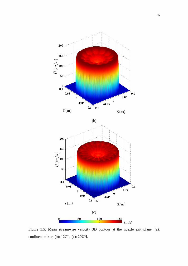
Figure 3.5: Mean streamwise velocity 3D contour at the nozzle exit plane. (a):

confluent mixer; (b): 12CL; (c): 20UH. ········································· 55

Figure 3.6: Time-averaged mean streamwise velocity contour for the three cases

along jet center plane. (a): confluent mixer; (b): 12CL; (c): 20UH. ········· 56

Figure 3.7: Center-line mean streamwise velocity. Blue line: confluent mixer;

green line: 12CL; red line: 20UH. ················································ 57

Figure 3.8: Time-averaged mean turbulent kinetic energy contour. (a): confluent

mixer; (b): 12CL; (c): 20UH. ····················································· 58

Figure 3.9: Non-dimensional center-line mean turbulent kinetic energy. Blue line:

confluent mixer; green line: 12CL; red line: 20UH. ··························· 58

Figure 3.10: Transwise views of mean streamwise velocity contour at different

streamwise locations. From left to right: confluent mixer, 12CL, 20UH; (a):

at mixer exit plane; (b): at nozzle exit plane; (c): 1Dj downstream of the

nozzle exit; (d): 2Dj downstream of the nozzle exit; (e): 3Dj downstream of

the nozzle exit; (f): 4Dj downstream of the nozzle exit.······················· 60

Figure 3.11: Downstream plume survey of mean streamwise velocity across

transverse cross-section of the jet at different downstream locations. (a):

confluent mixer; (b): 12CL; (c): 20UH. Dark blue line: at nozzle exit plane;

green line: 0.2Dj downstream of the nozzle exit; red line: 0.5Dj downstream

of the nozzle exit; light blue line: 1Dj downstream of the nozzle exit; purple

line: 3Dj downstream of the nozzle exit; brown line: 5Dj downstream of the

nozzle exit. ··········································································· 62

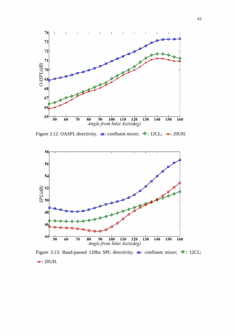
Figure 3.12: OASPL directivity. : confluent mixer; : 12CL; : 20UH. 63

Figure 3.13: Band-passed 120hz SPL directivity. : confluent mixer; :

12CL; : 20UH. ·································································· 63

Figure 3.14: Band-passed 1200hz SPL directivity. : confluent mixer; :

12CL; : 20UH. ·································································· 64

Figure 3.15: Band-passed 4500hz SPL directivity. : confluent mixer; :

vii

12CL; : 20UH. ·································································· 64

Figure 4.1: Instantaneous total velocity contours of the four mixers. (a):

confluent mixer; (b): 20UH; (c): 20MH; (d): 20DH. ·························· 75

Figure 4.2: Close-up view of instantaneous vorticity inside the four nozzles. (a):

confluent mixer; (b): 20UH; (c): 20MH; (d): 20DH. ·························· 77

Figure 4.3: Lambda 2 criterion iso-surface for the four mixers. (a): confluent

mixer; (b): 20UH; (c): 20MH; (d): 20DH. (iso-surface value = -100) ······ 78

Figure 4.4: Mean streamwise velocity 3D contour at the nozzle exit plane. (a):

confluent mixer; (b): 20UH; (c): 20MH; (d): 20DH. ·························· 80

Figure 4.5: Time-averaged mean streamwise velocity contour for the four cases

along jet center plane. (a): confluent mixer; (b): 20UH; (c): 20MH; (d):

20DH. ················································································· 81

Figure 4.6: Center-line mean streamwise velocity. Dark blue line: confluent

mixer; green line: 20UH; red line: 20MH; light blue line: 20DH. ·········· 82

Figure 4.7: Time-averaged mean turbulent kinetic energy contour. (a): confluent

mixer; (b): 20UH; (c): 20MH; (d): 20DH. ······································ 83

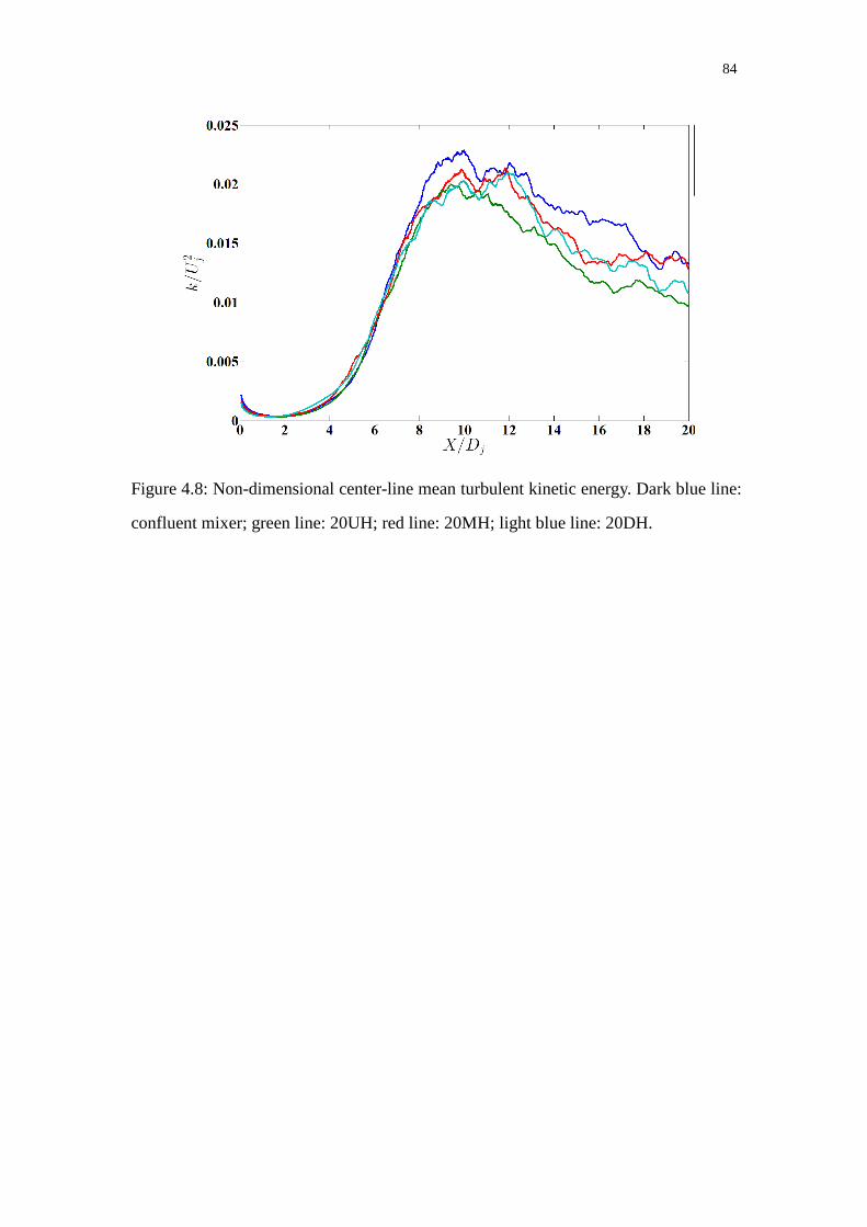
Figure 4.8: Non-dimensional center-line mean turbulent kinetic energy. Dark

blue line: confluent mixer; green line: 20UH; red line: 20MH; light blue line:

20DH. ················································································· 84

Figure 4.9: Transwise views of mean streamwise velocity contour at different

streamwise locations. From left to right: 20UH, 20MH, 20DH; (a): at mixer

exit plane; (b): at nozzle exit plane; (c): 1Dj downstream of the nozzle exit;

(d): 2Dj downstream of the nozzle exit; (e): 3Dj downstream of the nozzle

exit; (f): 4Dj downstream of the nozzle exit. ···································· 86

Figure 4.10: Downstream plume survey of mean streamwise velocity across

transverse cross-section of the jet at different downstream locations. (a):

confluent mixer; (b): 20UH; (c): 20MH; (d): 20DH. Dark blue line: at

nozzle exit plane; green line: 0.2Dj downstream of the nozzle exit; red line:

0.5Dj downstream of the nozzle exit; light blue line: 1Dj downstream of the

viii

nozzle exit; purple line: 3Dj downstream of the nozzle exit; brown line: 5Dj

downstream of the nozzle exit. ··················································· 88

Figure 4.11: OASPL directivity. : confluent mixer; : 20UH; : 20MH;

: 20DH. ············································································ 89

Figure 4.12: Band-passed 120hz SPL directivity. : confluent mixer; :

20UH; : 20MH; : 20DH. ·················································· 89

Figure 4.13: Band-passed 1200hz SPL directivity. : confluent mixer; :

20UH; : 20MH; : 20DH. ·················································· 90

Figure 4.14: Band-passed 4500hz SPL directivity. : confluent mixer; :

20UH; : 20MH; : 20DH. ·················································· 90

ix

NOMENCLATURE

Roman Symbols

A Area

ci Particle speed

Cp Specific heat capacity at constant pressure

D Diameter

Dmp Diameter of the mixing plane

fi Distribution function

Fi Equilibrium distribution function

Hmp Height of mixing plane

Hm Height of mixer lobe

L Nozzle nominal mixing length

Lchar Characteristic length

Ls Scalloping depth

m Mass

M Mach number

NPR Total pressure ratio

NTR Total temperature ratio

p Pressure

pchar Characteristic pressure

R Ideal gas constant

S Symmetric parts of the velocity gradient tensor

r Radial distance

T Lattice temperature

Tchar Characteristic temperature

t Time

tts Simulation time

x

ts Simulated physical time in one time step

U Streamwise velocity

Vchar Characteristic velocity

v Mean velocity of flow

wi Weight parameter for lattice model

x,y,z Cartesian coordinates

Greek Symbols

t Time resolution

r Simulation resolution

k Turbulent kinetic energy

Fluid density

char Characteristic density

u(x,t) First order moment of fluid velocity

Wavelength

Relaxation time

Kinematic viscosity

char Characteristic viscosity

Energy dissipation rate

Ω Anti-symmetric parts of the velocity gradient tensor

u Velocity gradient tensor

Superscripts, Subscripts, and Accents

( )i Direction of particles in a lattice model

( )j Jet properties

( )f Fan stream properties

( )c Core stream properties

( )0 Stagnation properties

( )s Static properties

xi

( )amb Ambient condition

Time averaged mean value

Flow rates

Abbreviations

LDV Laser Doppler Velocimetry

RANS Reynolds Averaged Navier-Stokes

LES Large Eddy Simulation

DNS Direct Numerical Simulation

FWH Ffowcs-Williams- Hawkings

CFD Computational Fluid Dynamics

LBM Lattice Boltzmann Method

LBE Lattice-Boltzmann Equation

BGK Bhatnagar-Gross-Krook

SRT Single Relaxation Time

RNG Renormalization Group

VLES Very Large Eddy Simulation

OASPL Overall Sound Pressure Level

SPL Sound Pressure Level

CONF Confluent mixer

12CL 12-lobe, unscalloped, low-penetration mixer

20UH 20-lobe, unscalloped, high-penetration mixer

20MH 20-lobe, mediumly-scalloped, high-penetration mixer

20DH 20-lobe, highly-scalloped, high-penetration mixer

CAD Computer Aided Design

STL Stereolithography

VR Variable Resolution

dB Decibel

BPR Bypass Ratio

xii

ABSTRACT

The growing stringency of community noise regulations for commercial turbo-fan

engines requires the development of effective jet noise suppression configurations.

The lobed mixer has been previously found to be an effective noise reduction device

for medium or low bypass engines typical of regional jet aircraft applications. The

large number of geometrical design parameters for lobed mixers precludes trial and

error experimental studies. In this study, a robust computational tool was used to

investigate the effects of lobe number, penetration depth and scalloping depth on the

sound radiated from a lobed mixer. The near field sound and flow were simulated

using a flow solver based on the Lattice Boltzmann Method (LBM). The far-field

radiated sound was predicted using the Ffwocs William-Hawkings (FWH) surface

integral method. The Reynolds number based on jet diameter was 1.36×106 and the

peak Mach number reached 0.5. The low-Mach setting was to abide by the constraints

of the 19-stage LBM algorithm used in this study, with operating conditions selected

to best approach the operating conditions of actual engines. The effects of an outer

mean flow to simulate forward flight were not included.

Two groups of one quarter scale mixers were selected for investigation. Flow

results and statistics were obtained. Plume survey data was obtained across transverse

cross-sections of the jet at different downstream locations. Far-field overall sound

pressure level (OASPL) and sound pressure level (SPL) directivity results were

obtained. All lobed mixers configurations were found to be quieter than the baseline

confluent mixer.

The results showed that a greater lobe number and a greater penetration depth

leads to lower low-to-mid frequency noise, and relatively higher sound pressure levels

at high frequency at locations far downstream. Lobed mixers were found to decrease

the sound pressure level at mid frequencies, and to significantly decrease noise

emissions at low frequencies.

xiii

The introduction of scalloping did not provide the same low-frequency noise

reduction advantage as unscalloped mixers, but yielded noise reduction benefits at

low frequencies compared to the baseline case. Deep scalloping tended to trade off

low-frequency noise suppression for a noise decrease at high frequencies. The SPL

directivity indicated the angle of maximum emissions changed with scalloping depth.

The results were found to be in qualitative agreement with published experimental

data.

xiv

Résumé

Les récentes mesures prises afin de règlementer le bruit provenant des

turboréacteurs à double flux nécessitent le développement de nouvelles configurations

de tuyères pour réduire le bruit de ces moteurs. Il a déjà été démontré que les

mélangeurs lobés peuvent aider à réduire les émissions sonores. La construction des

mélangeurs à lobes comprend un grand nombre de paramètres géométriques, ce qui

rend difficiles les approches d’optimisation expérimentales pour trouver la

configuration idéale. Dans la présente étude, un logiciel a été utilisé pour analyser

l’effet du nombre de lobes sur les niveaux de bruit. Les effets de la largeur et

profondeur des lobes, et la profondeur des festons furent aussi étudiés. L’écoulement

et le bruit à proximité du jet ont été simulés en utilisant un logiciel basé sur la

méthode de Boltzmann sur réseau (MBR). Le bruit en champ lointain a été prédit en

utilisant la méthode analogique de Ffwocs-Williams et Hawkings. Le nombre de

Reynolds, basé sur le diamètre du jet, était de 1.36x106, et le nombre de Mach

maximum était 0.5. Le nombre de Mach est limité en raison de restrictions inhérentes

au schéma de calcul MBR utilisé. Les paramètres de l’écoulement ont été choisis pour

approcher les conditions de vol de vrais moteurs. Les effets d’un écoulement

extérieur pour simuler le mouvement de l’avion ne furent pas pris en considération.

Deux groupes de mélangeurs à l’échelle d’un quart ont été sélectionnés pour cette

étude. Les résultats et statistiques de l’écoulement instantané et moyenné ont été

obtenus. Les données du panache ont été obtenues sur des coupes transversales à

plusieurs positions en aval du jet. Les niveaux de pression acoustiques pondérés et la

directivité du bruit ont été obtenus. Tous les résultats indiquent que les mélangeurs à

lobes étudiés sont plus silencieux que le mélangeur confluent standard, tel qu’attendu.

Les résultats suggèrent qu’un plus grand nombre de lobes et une profondeur de

pénétration plus prononcée sont préférables vis à vis les fréquences moyennes et

basses, au prix d’émissions accrues en aval pour les fréquences élevées. Les

mélangeurs à lobes semblent produire moins de bruit aux fréquences moyennes, mais

xv

la réduction est plus prononcée pour le bruit à basse fréquence.

Les mélangeurs avec festons n’ont pas réduit le bruit à basse fréquence autant que

les mélangeurs sans festons. Ceci semble indiquer que les festons à haute-profondeur

sont préférables aux fréquences élevées et non aux basses fréquences. La directivité

du bruit suggère un décalage de crête associé à la variation de la profondeur des

festons. Les résultats obtenus sont en bon accord qualitatif avec les données

expérimentales publiées dans la littérature.

1

Chapter 1 Introduction

1.1 Motivation

Government and airport regulations have implemented stricter regulations for

aircraft noise emissions over the past decades. Aircraft noise has been found to cause

physical and mental damage to the communities surrounding airports1. In the United

States, a goal was stated in 1997 that the perceived noise levels of future subsonic

aircraft would be reduced by a factor of two by 2007 and by a factor of four by 20222.

Jet noise is the dominant contributor to aircraft noise at takeoff. Noise reduction at the

source requires a deep understanding of the turbulent flow processes responsible for

the generation of sound radiated in the surrounding environment. Jet noise still

remains one of the most elusive problems in aeroacoustics due to the complexity of

the flow-generated sound processes.

For the case of subsonic single stream jets, noise is created by the turbulent

mixing of the jet stream with the ambient air. For coaxial jets, additional noise may be

generated by the mixing of the primary and secondary flows. Complex jet

configurations can have additional mixing enhancement devices, such as lobed mixers

or chevrons. Currently, there is no well developed industrial design tool for the

prediction of the noise characteristics resulting from complex jet flows. As a result,

the jet noise levels of modern turbofan jet engine configurations can only be

determined through expensive experimental testing after they have been designed and

built. The current study focused on noise predictions from jets with internal forced

lobed mixers which are currently used in regional jet aircraft.

2

1.2 Lobed Mixers and Key Parameters

Reduction of jet noise has been sought earlier by mixing the hot core flow and the

cooler fan flow before they exit through the nozzle. A more uniform flow at the nozzle

exit plane leads to reduced noise levels. Uniform flow at the nozzle exit plane yields

better cruise thrust efficiency thermodynamically than partially mixed flow or

separate unmixed flow nozzle systems. That is the primary reason for mixing the

flows internally. However, the overall noise benefit and penalty resulting from

internal mixing to achieve the uniform exit flow is not well understood. The actual

level of noise abatement realized in a specific application must be critically related to

the manner and extent to which internal mixing is achieved. So far various kinds of

devices proposed include confluent mixers, vortex generators, chevrons, exhaust tabs,

diverters and lobed mixers. Among these devices tested, the lobed mixer configuration

has been found to yield significantly enhanced mixing with acceptable pressure

losses.

A lobed mixer is basically a splitter plate with a convoluted trailing edge which

alternately diverts the upper and lower streams into the lobe troughs. The key

parameters of a lobed mixer nozzle include lobe number, lobe penetration, scalloping

shape, perimeter of the trailing edge and mixing length.

The lobe number is directly related to the wetted perimeter. By increasing the

lobe number in the mixer, the interface area between the two flow streams is increased,

which leads to an overall increase in turbulent mixing. However, this process is not

entirely straightforward. Because all mixers must fit within the same duct

cross-sectional area, increasing the number of lobes produces a corresponding

decrease in lobe width and in diameter of the axial vortex shed from each lobe

sidewall. The resulting changes in vortex growth, diffusion, and interaction

substantially alter and complicate the mixing process. The possible acoustic benefit is

offset by increases in skin friction and total pressure loss, which adversely affect

thrust production. Other factors such as weight, blockage due to the lobe metal

thickness, and the manufacturing of the mixers also need to be considered.

3

The introduction of scalloping to the lobed mixer allows the two streams to

interact with each other gradually and further upstream. Because the two streams are

not parallel near the lobe sidewall, their radial velocity components give rise to axial

or streamwise vorticity shed from the leading edge of the scallop. Streamwise

vorticity enhances mixing between two streams compared with mixing only due to

Kelvin-Helmholtz type vortex-sheet instability.3,4

Scalloping should be designed such

that the vorticity is introduced gradually. The axial gradient at which net vorticity is

introduced into the flow should be smooth and gradually increasing, presumably

reducing the relatively high-frequency noise sources. In comparison, high-frequency

noise generation is expected for unscalloped mixers because the two streams merge

with each other suddenly after the exit of the mixer across the full height of the lobe,

the generation of high-frequency noise is expected. To minimize the dipole noise, the

scalloped edge should be shaped such that it acts as a trailing edge over its entire

length with respect to both streams around it.

1.3 Previous Experimental Studies of Lobed Mixers

1.3.1 Mixing Mechanisms

A combination of several lobed mixer design parameters significantly affects the

mixing process, thereby the associated noise generation.

It has been suggested that the mixing process in a lobed mixer is controlled by

three major factors4. These are the streamwise vorticity generated by lobe shape, the

increase in the interfacial area between the two fluid streams, and the Brown-Roshko

type structures that occur in any free shear layer due to the Kelvin-Helmholtz

instabilities. Manning5 attempted to isolate the effects of these three mechanisms. He

studied a flat plate as a baseline case and two different lobed mixers. Mixing

performance of the lobed mixer exceeded the performance of the convoluted plate by

an amount that increased with velocity ratio. At velocity ratios close to unity, the

increased mixing was mainly due to the increased contact area, whereas the

4

streamwise vorticity had a larger role at a velocity ratio of two.

Paterson6,7

studied subsonic flow issuing from a lobed nozzle for both cold and

heated flows. Detailed pressure and temperature data were obtained as well as three

dimensional laser Doppler velocimetry (LDV) measurements. Paterson found that

large-scale secondary flows, set up by the nozzle, produced streamwise vortices of

low intensity with a length scale on the order of the nozzle radius. Also, a horseshoe

vortex on the order of the lobe half-width was found in the lobe troughs. The

respective contribution of these flow features to the overall mixing process was not

clear, but the secondary flow vortices were argued to be dominant because of their

much greater size. Werle et al.8 found that the vortex formation process was an

inviscid one. Also, the mixing process was proposed to take place in three basic steps:

the vortices formed, intensified, and then rapidly broke down into small scale

turbulence. In effect, the lobed mixer was thought to act as a “stirrer” initially to mix

the flow, until the rapid breakdown of the vortices produced small scale, and possibly,

molecular mixing. Eckerle et al.9 used a two component LDV to study mixing

downstream of a lobed mixer at two velocity ratios. They determined that the

breakdown of the large scale vortices, and the accompanying increase in turbulent

mixing, was an important part of the mixing process. This vortex breakdown occurred

further upstream for a velocity ratio of 2:1 than for 1:1. Barber et al.10

studied both

analytically and experimentally three different two-dimensional lobed mixers.

Performing a one-dimensional inviscid analysis to predict lobe circulation and

geometrical scaling relations produced results in reasonable agreement with their data,

further emphasizing the inviscid nature of the overall large scale mixing process. One

of the conclusions of that study was that lobed mixers with parallel side walls

produced higher streamwise circulation than lobes with sinusoidal or triangular shapes.

The close proximity of the walls in the lobe peak region for the triangular shapes

created thicker boundary layers which reduced the effective lobe height and therefore

reduced circulation. A detailed study by McCormick11

revealed several more details

of the flow patterns downstreams of a lobed mixer. Extensive flow visualizations and

5

three-dimensional velocity measurements showed that the interaction between

Kelvin-Helmholtz vortices and the streamwise vortices produced high levels of

mixing. The streamwise vortices pinched off the normal vortices, thus enhancing the

stirring effect in the flow. This pinching caused the normal vortices to merge within

1.5 lobe heights downstream, where they were observed to break down shortly

thereafter, leading to intense turbulent mixing. Another interesting observation by

McCormick was that the scale of the normal vortices shed from the lobed mixer was

about 25% of that shed from a planar baseline case. From this, McCormick and

Bennet12

inferred that the lobed mixer introduced smaller scales into the flow stream

further upstream, which might enhance molecular mixing.

1.3.2 Evaluation of Lobed Mixers

Experimental research on lobed mixers has been extensive in the past few

decades. Pioneering work by Frost13

and Hartmann14

showed the theoretical thrust

gain for ideal mixing and presented results from turbofan engine scale model tests

with nominal low bypass ratios. Since then, both far-field noise data for lobed

mixers15

and detailed measurements of aerodynamic properties16,17,18

have been

reported in the literature. Couch et al.19

and Packman et al.15

reported that jet noise

could be reduced by mixing the turbofan engine fan and primary streams. Shumpert20

investigated four types of internal mixers (confluent, injection, vortex generator, and

lobed mixer) for turbofan engines with a nominal engine airflow bypass ratio of six.

The experimental results were presented in terms of mixer nozzle pressure losses,

mixing effectiveness, thrust gain, and primary thrust recovery. It was concluded that

the lobed mixer favored rapid mixing of the two streams, and 70% of the ideal thrust

gain was achievable. Kuchar’s experimental study17

on scale model performance first

revealed the qualitative correlation between lobed mixer geometric properties and the

engine performance. Their conclusion was that scalloping enhanced mixing with

essentially no increase in mixer pressure loss. Kozlowski and Kraft 21

later conducted

a similar study. They found that increasing the lobe number and radial penetration of a

6

lobed mixer within a certain range offered overall performance improvement. The

introduction of scalloping was also found to be beneficial. Barber et al.10, 22, 23

showed that a forced mixer reduced the exit jet velocity without significant thrust

penalties for turbofan engines. Barber et al. also established the inviscid nature of the

streamwise vortices formation at the mixer trailing edge. They compared streamwise

circulation measurements near the trailing edge with analytical results based on the

principle of two-dimensional continuity within the penetration region, and good

agreement was obtained. Booher et al.24

showed that lobed mixers with high

penetration yielded substantial performance improvements at typical subsonic

cruising relative to an unmixed nozzle configuration. According to their experimental

results, the generation of streamwise vorticity and the rapid mixing of the fan and core

streams downstream of the mixer yielded very high mixing effectiveness values with

low total pressure losses. In an acoustic study of lobed mixers on a high bypass ratio

engine, Meade25

showed that internal forced mixing significantly reduced jet noise

compared to internal confluent mixing. Publications by Presz et al.26, 27, 28

again

indicated that the enhanced mixing between the core and the bypass flows caused by

the lobed mixer not only reduced jet noise, but also provided some gains on net thrust.

Nevertheless, a systematic study on the effects of lobed mixer parameters is not

practical without predictions from numerical simulations.

1.4 Jet Noise Prediction Methods

Computational simulations have been established as a primary tool for recent jet

noise sound generation studies. Three basic approaches to computational

aeroacoustics are the direct, the semi-empirical, and the indirect approach.

In the direct approach, the complete and fully coupled compressible Navier-Stokes

equations are solved. The computational domain includes both the source region and

the far-field observer. Sound generation and propagation phenomena are part of the

solution. Because the acoustic perturbations are very small compared to the mean

flow properties, high-order, low-dissipative, and low-dispersion schemes are required

7

to provide reliable results. Therefore, the direct approach is usually very expensive

and suitable only for fundamental studies and academic configurations.

In the semi-empirical approach, a steady or unsteady Reynolds Averaged Navier

Stokes (RANS) computation is performed to obtain information about turbulence

length and time scales. This information is then transformed into sound-source spectra

using empirical relations. This approach is inexpensive, but the reliability of the

results is heavily dependent on the validity and accuracy of the empirical relations in

the case being considered.

The indirect approach consists of two steps. The first step is to perform a detailed

and accurate flow simulation in the near-field where all possible sources are contained

in the computational domain using large eddy simulation (LES) or direct numerical

simulation (DNS). The second step is to use an acoustic analogy method such as

Lighthill’s acoustic analogy, the Ffowcs-Williams-Hawkings (FWH) method, or the

Kirchhoff surface integral method to obtain the far-field noise. This approach is less

expensive than the direct approach and provides valuable information about the

overall sound level and directivity in the far-field. Limitations include the neglect of

flow-sound interactions and scattering through shear layers. In the present study, the

indirect approach was adopted. The investigation was categorized into near-field flow

simulation and far-field noise prediction.

1.4.1 Near-field Simulations

Previous researchers have performed calculations to capture the near-field flow

features generated by lobed mixers. Povinelli and Anderson29

developed a computer

code that could predict the complex three-dimensional temperature contours within

the mixing duct, however, their prediction largely depended on the accurate

knowledge of the 3D velocity field at lobe exit for use as inlet boundary conditions.

To tackle this problem, Barber et al.30,31

and Koutmos and McGuirk32

modeled the

lobe flow itself. Malecki and Lord33

and Abolfad and Sehra34

later performed an

analytical modeling of the mixer utilizing the full Navier-Stokes analysis and

8

provided some insight into the design of lobed mixers. In the last two decades, some

researchers investigated lobed mixer flows using RANS computational fluid dynamics

(CFD) analysis. Barber et al.35

performed RANS simulations of jet flows with lobed

mixers. Salman et al.36,37

used both structured and unstructured grids to study lobed

mixer jet flows. Garrison38

carried out RANS calculations based on the WIND flow

solver with a two-equation turbulence model, and the results were able to capture

some features of lobed mixer flows.

Most numerical methods now involve the solution of some form of the basic

equations of motion using finite difference schemes. With the continuous

improvements in computing power, the application of DNS is now feasible in some

cases39,40

. The approach involves the simulation of the flow dynamics for all the

relevant turbulence scales. Hence it requires no turbulence model. The wide range of

time and length scales present in turbulent flows and the current computational

resources limit the use of DNS for high Reynolds number flows. LES involves direct

computation of the large scales, in conjunction with sub-grid scale models. It is

assumed that the large scales in turbulence are generally more energetic than the small

scales and are affected by the boundary conditions directly. In contrast, the small

scales are more dissipative, weaker, and tend to be more universal in nature. Most

turbulent jet flows that occur in experimental or industrial settings are at high

Reynolds numbers. LES methods for high Reynolds number flows cost a fraction of

DNS. One of the first uses of LES as an investigative tool for jet noise prediction was

carried out by Mankbadi et al.41

They performed a simulation of a low Reynolds

number supersonic jet and applied Lighthill’s analogy42

to calculate the far-field

noise. Lyrintzis and Mankbadi43

used Kirchhoff’s method with LES to compute the

far-field noise. Other numerical studies44,45,46

were then carried out by investigators at

higher Reynolds numbers. A comprehensive overview of applications of LES to jet

noise prediction was given by Uzun47

. In general, the results have been found to be

accurate, and in good agreement with experimental results.

However, the aforementioned simulations did not include a nozzle in the

9

computational domain, which precluded possible dipole contributions from the nozzle

surfaces. Instead, ad hoc inflow conditions that typically include random Gaussian or

pipe flow simulation output data as forcing were specified to mimic the nozzle exit

plume. Although the exclusion of the nozzle reduces computational costs, inflow

forcing tends to result in higher noise levels in the far-field compared to experiments.

The inclusion of the nozzles in LES simulations is rather recent, and the works of

Anderson et al.48

, Paliath and Morris49

, Schur et al.50

, and Uzun and Hussaini51

are

the most notable. The simulation results obtained following the inclusion of the nozzle

geometry did improve the far-field noise prediction but at the expense of

computational cost. Even if the computational expense with the addition of the nozzle

is acceptable, the setup for these simulations includes tedious body-fitted meshing for

complex geometries. Thus, despite recent progress in computational aeroacoustics,

detailed LES studies remain largely confined to academic jet configurations.

Hence, computational tools with high accuracy, high efficiency, stability, and

relatively low cost have to be developed to uncover the flow and noise characteristics

resulting from complex jet flows, such as lobed mixer flows. The tool based on the

Lattice Boltzmann Method (LBM) is a potential candidate in addition to

Navier-Stokes based methods, and it was employed in the present study.

Recent advances have been made in kinetic based methodologies such as the

lattice-Boltzmann method (LBM). These methods have been shown to be accurate for

the simulation of complex fluid phenomena52

. While Navier-Stokes equations solve

the macroscopic properties of the fluid explicitly, LBM solves the Lattice-Boltzmann

equation (LBE) by explicitly tracking the development of particle distribution

functions either at the mesoscopic or the microscopic scale. Through the use of the

Chapman-Enskog expansion53

, the LBE has been shown to recover the compressible

Navier-Stokes equation at the hydrodynamic limit52, 54, 55

. The conserved variables

such as density, momentum and internal energy are obtained by performing a local

integration of the particle distribution. The LBM has been recently applied to

aeroacoustic problems. Lew et al.75

applied LBM to study the far-field noise

10

generated from an unheated round jet of Mach 0.4. The predicted far-field sound

pressure levels were within 2 dB from experimental data. Lew et al.56

conducted a

study to predict the noise radiation from a round jet with impinging microjets using

LBM. The results were found to be in qualitative agreement with experimental

observations. Habibi et al.57

used LBM to investigate the aeroacoustic problem of

low-Mach heated round jets. Qualitative comparison between simulated results and

experimental data supported the viability of the LBM schemes application. More

detailed background of LBM is discussed in section 1.5.

1.4.2 Far-field Sound Predictions

In the indirect approach, the flow field data is usually post-processed using the

acoustic analogy to determine the far-field sound. The acoustic analogy was first

formed by Lighthill42

through the derivation of an equation to describe

aerodynamically generated noise by rearranging the Navier-Stokes equations. In

particular, Lighthill derived the acoustic analogy by combining the continuity and

momentum equations. He then formed a wave equation on the left-hand side and

moved all other terms to the right-hand side. In this form, the wave operator on the

left-hand side represents the propagation of the sound and the terms on the right-hand

side are regarded as known source terms that are responsible for the generation of the

sound. Further developments have been made to the standard acoustic analogy

developed by Lighthill to account for noise sources that are embedded in a mean flow.

Lilley derived another acoustic analogy58

, and the governing equation is linearized for

a parallel sheared mean flow, which is representative of the mean flow in a jet. The

advantage of this approach is that in addition to the propagation of the sound it also

accounts for the refraction of sound waves in the jet mean flow.

In the current study, a modified porous FWH surface integral acoustic method59

was used to predict the far-field noise. An FWH formulation is the generalization of

Lighthill’s equation to account for the effect of a moving solid surface. The

formulation source terms include monopoles, dipoles, and quadrupoles. The surface

11

integral method follows the description of Lyrintzis & Uzun60

and Lyrintzis61

. For

simplicity, a continuous stationary control surface around the turbulent jet was used.

Details regarding the numerical implementation of the FWH method can be found in

Uzun47

.

1.5 Lattice-Boltzmann Method

The Lattice-Boltzmann equation has the following form52, 53

:

)),,(),((),(),( txFtxft

txftttcxf iiiii

(1.1)

where the distribution function fi (x,t) yields the number density of kinetic particles at

position, x, with a particle velocity ci in the i direction at time t. The left-hand side of

(1) computes the particle advection from one center cell to another whereas the

right-hand side of (1), known as the collision operator, represents the relaxation of the

particles. The Bhatnagar-Gross-Krook (BGK) approximation62

is used to relax the

equilibrium distribution function Fi (x,t). The relaxation time , however, is related

to the kinematic viscosity, , such that = ( + t )/T. This relation is also

commonly referred to as single relaxation time (SRT). The conservative macroscopic

variables, such as density and momentum density, are obtained through the zeroth and

first-order moments of the distribution function:

,),(),( i

i txftx .),(),( i

ii txfctxu

(1.2)

The pressure is obtained using the equation of state for an ideal gas with the

assumption that the gas constant is taken to be unity. This can be expressed as p= T.

In addition, the LBM approach recovers the compressible, viscous Navier-Stokes

equation in the hydrodynamic limit for wavelengths and frequencies

To recover the macroscopic hydrodynamics, Fi(x,t) must be chosen in

such a way that the essential conservation laws are satisfied and the resulting

macroscopic equations are Galilean invariant. In the three-dimensional situation, one

of the common choices is the D3Q19 model63

shown in Figure 1.1:

12

,26

)(

22

)(1 2

23

3

2

2

2

2

u

T

uc

T

uc

T

u

T

uc

T

ucwF iiii

ii

(1.3)

where wi has the weighting parameters of 1/18 in the 6 coordinate directions, 1/36 in

the 12 bi-diagonal directions and 1/3 for the ‘rest’ particle. T is the lattice temperature,

which is set to 1/3 for isothermal simulations. The LBM used in this study has been

shown to be second-order accurate in time and space64

.

To account for the presence of solid boundaries in the simulation, the no-slip

boundary condition used a simple particle bounce back and reflection process on a

solid surface64

. In addition, an improved volumetric boundary scheme for arbitrary

geometries has been devised and implemented to accurately control and govern the

momentum flux across the boundary. Further details regarding the handling of solid

geometries can be found in references64, 65

.

To include the unresolved turbulent scales, an eddy viscosity turbulence model

was used. Specifically, the commercial code used in this study employed the

two-equation k- renormalization group (RNG) turbulence model to compute the

turbulence viscosity with the addition of a swirl corrector to model part of the large

scale structures. This methodology is also commonly referred to as very large eddy

simulation (VLES). This procedure has been argued to be analogous to an LES66

.

The potential advantages of LBM over the conventional Navier-Stokes solvers

include: 1) linearity of the convection operator (Equation (1.1)) due to the kinetic

nature of the LBE method; 2) easy calculation of the strain rate from the

non-equilibrium distribution function; 3) suitability for complex geometries, due to

the absence of Jacobians to compute grid metrics; 4) ease of parallelization for large

to massive supercomputing architectures due to its simplicity in terms of form.

The most notable disadvantage is that the LBM does not recover flow physics

correctly for cases with high Mach numbers (M > 0.5). Efforts are being made to

extend the current LBM for higher Mach number jet flows. Recently, Sun and Hsu67

used an LBM technique to study a shock tube problem and obtained good results

compared to the Reimann solution. Shan et al.68

and Chen et al.69

have laid a firm

13

theoretical groundwork to efficiently extend the LBM to higher Mach numbers and

arbitrary Knudsen numbers. Recently, Li et al.70

devised a modified Boltzmann

equation and applied it to a 2D aeroacoustic benchmark problem. They obtained good

results and showed that their methodology is valid up to a Mach number of 0.9.

1.6 Research Objectives

Investigating the impact of various parameters of a lobed mixer on the generated

noise requires a systematic study; however, the underlying mixing mechanism is

affected by only three main factors4. Through a comprehensive study of several key

parameters, some understanding of these underlying physical mechanisms can be

obtained and used for a better mixer design. The objective of this study is, therefore,

to investigate the three most important lobed mixer parameters on noise suppression:

lobe number, penetration depth, and scalloping effects. One group of three mixers was

selected with the aim to uncover the compound effect of increased lobe number and

penetration depth, which is equivalent to the effect of increased interface area. The

second group of four mixers was chosen to investigate the far-field sound pressure

level differences caused by different scalloping depth. Another goal of the study is to

showcase the capacity and applicability of the LBM scheme in simulating complex jet

flow.

1.7 Organization of the Thesis

This thesis is organized as follows. In chapter 2, five different mixer-nozzle

configurations are introduced, and the setting of grid distribution and measurement

windows in the simulation is discussed. The characteristic parameters, initial

condition, boundary conditions, and the use of forcing function are also presented. In

chapter 3, three mixers are selected to study the compound effect of lobe number and

penetration depth. Both instantaneous and time-averaged flow results and statistics are

presented. Plume survey data is given. Overall sound pressure level (OASPL) and

sound pressure level (SPL) directivity results are shown for the three mixers to

14

analyze the far-field radiated noise. In chapter 4, three scalloped mixers along with a

confluent mixer are investigated for the aerodynamic and acoustic effect of scalloping.

The same set of simulation results as those in chapter 3 is given and compared among

the four mixers. Chapter 5 summarizes the results and gives an outlook on future

work.

15

Figure 1.1: Schematic of the D3Q19 LBM Model71

.

16

Chapter 2 Numerical Procedures

In this chapter, the five selected mixer configurations are briefly described. The

configuration of the computational grid distribution and measurement window is

discussed. The characteristic parameters, initial condition, and adjusted inflow

boundary conditions are given. Although the simulations were conducted without heat

transfer, a verified approach was applied to approximate heated flow conditions with

isothermal conditions. The use of artificial forcing techniques is presented at the end.

The simulations were performed using a commercial LBM code (i.e., PowerFLOW

4.3d) for a maximum Mach number below the upper limit of 0.5.

2.1 Lobed Mixer and Nozzle Models

Five lobed mixer-nozzle geometries were extracted from a NASA report72

:

confluent mixer (CONF); 12-lobe, unscalloped, low-penetration mixer (12CL);

20-lobe, unscalloped, high-penetration mixer (20UH); 20-lobe, mediumly scalloped,

high-penetration mixer (20MH); and 20-lobe, highly scalloped, high-penetration

mixer (20DH). Figure 2.1 shows the mixer-nozzle configurations. All mixer-nozzle

configurations have common inner flow lines and consist of three parts: nozzle, mixer,

and center-cone. Mixer key parameters are listed in Table 2.1. Figures 2.2 and 2.3

illustrate the mixer-nozzle configuration and five test models. The selected nozzle

geometry is the same for all five configurations. The converging nozzle diameter

decreases from about 261.37mm at the inlet to 184mm at the nozzle exit plane. The

nozzle has a nominal mixing length, L, of 279.4mm which yields a mixing length to

mixing plane diameter ratio (L/Dmp) of about 1.10.

The confluent mixer was used as the baseline reference configuration. Acoustic

data obtained from the previous tests72,73

confirmed that aggressive, high-penetration,

17

unscalloped mixer configurations suppressed low-frequency noise emissions, which

are characteristic of unmixed, coaxial turbofan exhausts, but also produced greater

emissions at higher frequencies. Previously presented data74

for scalloped sidewall

mixers shows that they reduced low frequency emissions without incurring a penalty

at the higher frequency regimes. Hence, it can be inferred that the scalloping on the

mixer sidewall can be beneficial to the overall sound pressure level reduction. This is

the reason why 20UH, 20MH, and 20DH mixers were included in this study. These

three mixers were designed for NASA tests72

and varied parametrically in the

scalloping depth and shape while holding all other parameters fixed. The purpose of

studying this group of mixers is to discover the impact of different sidewall scalloping

on far-field sound radiation. Meanwhile, the 12CL mixer was selected to gauge the

combining effects of different lobe number and penetration depth.

The mixer-nozzle solid boundaries were incorporated into the computational

domains as follows. A solid model was created using CAD software and then

imported into the code as a stereolithography (STL) file format. The STL file

contained the information representing the surface features of a 3D body of the mixers.

The interaction between a surface mesh and a discrete voxel generated a surface

element. This element acted as a boundary lattice element that imposed a no-slip

boundary condition on the flow field via the bounce-back scheme which is utilized in

LBM56

. Despite the very complex shape of the lobed mixers, the LBM approach

allows relatively easy geometries import.

2.2 Geometries Configurations

2.2.1 Simulation Domain and Variable Resolution Regions

The dimensions of the computational domain were (x,y,z)=(37Dj, ±15Dj, ±15Dj).

The domain length was sufficiently long to include twice the length of the jet core, as

well as a sponge layer to dissipate and absorb the reflected acoustic waves. The

outermost contour in Figures 2.4 and 2.5 illustrates the outer boundary of the

18

computational domain.

The computational domain was partitioned into several variable resolution (VR)

regions to tailor the grid as needed to resolve the flow details and reduce

computational costs. This methodology is similar to grid-stretching techniques

typically employed in CFD. Figure 2.4 shows a side view of the computational

domain. Successive VR regions were concentric and cylindrical as shown in Figure

2.5, but the voxels are cubic. The second outermost rectangular bounding region

shows the inner boundary of the sponge layer. Sufficient spacing must be provided

between successive VR regions radially and in the streamwise direction. Simulation

with no spacing in the streamwise direction between VR regions usually causes “VR

tones” to be generated in the far-field pressure spectra. These tones can have very

significant levels of 15 dB above the underlying broadband spectral density levels75

,

and therefore bias the overall spectrum. Sufficient streamwise spacing between VR

regions eliminated these tones to a large extent. Each grid cell is called a “voxel”.

Hence, each VR region represented one grid resolution level and the VRs cascaded

outwards from the fine resolution region towards the coarse resolution region. The

voxel cell size between each successive VR region differed by a factor of two to keep

the lattice velocity directions consistent between VR interfaces. The domain included

a total of around 76 million voxels. The entire simulation domain was divided into

seven VR regions. To the same end, coarse VR regions further away from the jet

dissipated the outgoing traveling waves and thus acted as ‘sponge’ zones. In addition,

an anechoic sponge layer with depth equivalent to five jet diameters was inserted

between the two outermost rectangular VR regions to minimize acoustic wave

reflection. Close-up views of the VR regions near the nozzle geometry are shown in

Figures 2.6 and 2.7. Figure 2.8 shows the voxel distribution over the entire domain.

Figures 2.9 and 2.10 show a close-up view of the voxel distribution inside the nozzle.

Figure 2.11 shows the voxel distribution at the nozzle exit.

Inside the nozzle, voxels of size 4.25×10-4

m were distributed very close to the

solid boundaries of the nozzle, the mixer, and the center-body (Figures 2.9 and 2.10)

19

to accurately capture the boundary layer characteristics. A high resolution in regions

of high shear is required for accurate sound production modeling. The smallest voxel

size corresponds to approximately /Dj 0.09 which may be considered coarse for

wall-bounded flow studies. The ratio needed to resolve the duct boundary layers is at

least one order of magnitude lower without the implementation of a wall model,

which is prohibitively expensive. Although the adopted cell size did not fully resolve

the boundary layer details, a carefully selected artificial forcing technique was utilized

to perturb the flow within the boundary layer to achieve physical jet inflow conditions.

The forcing function used in this study is discussed in section 2.3.2. A VR region with

second resolution level was placed right off the finest level to act as a smooth

transition from the smallest to coarser grids in the outer region.

The shear layer is a major contributor to the far-field sound radiation due to the

large velocity gradients and turbulence levels. Possible flow separation downstream of

the center-body may also generate flow patterns with high turbulence intensity, which

also contribute to the far-field sound. A second finest VR level was therefore put at the

downstream of both the mixer and the center-body to resolve the shear layer, vortex

shedding and flow separation. A comparison between initial and later studies showed

a satisfactory improvement on the resolved flow pattern when the second finest VR

level (Figure 2.9) was added.

Outside the nozzle, two finest cylindrical VR regions were placed downstream of

the nozzle tip to capture the initial development of turbulence in the shear layer. In

addition, a larger VR region with third finest resolution level was located further

downstream of the nozzle exit to yield a smooth transition to the outer coarser VR

regions. Experience from previous simulations showed that the shear layer and vortex

shedding features generated from the mixer tip have their footprint downstream close

to the nozzle exit. Therefore a third VR level was added to properly cover that region

(Figures 2.6 and 2.9).

20

2.2.2 Measurement Windows

Two volume measurement windows and one surface measurement window were

used in the simulation. A rectangular streamwise measurement window with a

thickness of two lattice lengths was placed at the symmetric plane of the simulation

domain, as indicated in Figure 2.12. This measurement window was used to check the

flow evolution and convergence and to generate snapshots of transient and

time-averaged flow fields. The flow data was recorded every 100 time steps, from the

establishment of flow convergence to the end of the simulation. Meanwhile, a

cylindrical measurement window was inserted in the near field. The window had an

initial diameter of 2Dj and a diameter of 6Dj at the end. It started upstream of the

nozzle inlet and extended to the downstream of the FWH surface measurement

window, with a length of 22Dj. This measurement window was mainly used for the

analysis of the near flow field, such as the turbulence kinetic energy, the center-line

mean velocity decay rate, the plume survey, and the 3D Lamda-2 criteria isosurface.

Due to the large amount of data included in the measurement window at each frame,

the data was sampled every 500 time steps and recorded after the establishment of

flow convergence to the end of the simulation.

A surface measurement window was utilized for the near-field sound data

recording, as indicated in Figure 2.13. This surface acted as a porous control surface

in the FWH surface integral method. For simplicity, a continuous stationary surface

around the turbulent jet was used. The funnel-shaped control surface started slightly

upstream of the nozzle exit and had an initial diameter of 3Dj. It extended streamwise

over a distance of 21 Dj and had diameter of 18Dj at the end. The shape of FWH

surface was reasonable compared to previous simulations75

, and the size was large

enough to include the jet potential core. The entire surface remained in the same VR

level to avoid different data sampling rates and different resolved Strouhal numbers.

The end of the surface also managed to keep a reasonable distance from the VR

transition to avoid spurious noise source caused by the VR tones. No data recording

surface was present at the two ends of the FWH surface to avoid spurious sound

21

caused by interaction between the surface and vortices. Flow data was collected on

the control surface at every 87 time steps over a period of 500,000 time steps. The

sampling data was recorded after the first jet plume and the first reflected acoustic

wave exited the computational domain. Based on the variable resolution around the

control surface, and assuming that LBM required 12 cells per wavelength to

accurately resolve an acoustic wave, the maximum resolved frequency corresponded

to a Strouhal number of three.

2.2.3 Inlet and Outlet Geometry

As shown in Figure 2.14, two annular surfaces were located at the inlet of the

nozzle and were fitted into the fan and core inflow area to help impose the inlet

boundary conditions.

Six planar rectangular surfaces were located at the boundaries of the simulation

domain to help impose the outlet boundary conditions. The surface at the outlet of the

computational domain is shown in Figure 2.15 as an example.

Four ring-shape surfaces were extracted from the solid mixer-nozzle geometries

to help define the forcing for the inflow perturbation. The application of the forcing

was referred to the trip procedure used by Bogey & Baily76

, and the forcing surfaces

were placed close to the inlet with a length of approximately 0.1Dj. Figure 2.16 shows

the four surfaces used for the forcing of the nozzle, mixer (both upper and lower

surface), and center-body.

2.3 Parameters and Operating Conditions

2.3.1 Characteristic Parameters

The characteristic parameters used in all the simulations are listed in Table 2.2.

The values were used to establish a dynamic range for the simulation case. Table 2.3

shows the grids points used in each case.

The atmospheric pressure was selected as the characteristic pressure (pchar) when

22

specifying the initial and boundary conditions and calculating the characteristic

density ( char). It was assumed to be approximately in the average of the pressure

range encountered in the cases. The characteristic velocity (Vchar) was selected to be

the inflow velocity of the core stream. It was used to calculate the simulated Reynolds

number (Re). The detailed calculation of Vchar is discussed in section 2.3.2. The

characteristic temperature (Tchar) was selected by the usual isothermal test conditions.

It was also used to calculate char. The characteristic viscosity ( char) was chosen by

the air viscosity at Tchar. The characteristic length (Lchar) was selected to be the nozzle

exit plane diameter. The value was used to calculate the smallest grid size and the Re.

The resolution ( r) was defined as the number of the smallest grid points along the

characteristic length. It specified the size of grids and surfels in the case. The smallest

grid size was calculated as the ratio of Lchar and r. The value in this case was

selected after careful consideration of the trade-off between accuracy and computation

time. The flow Mach number is limited to values below 0.5 in the LBM scheme. In

this range, flow results are approximately independent of Mach number. The flow

field converges more rapidly when running a simulation at higher Mach number

because the particles comprising the digital fluid move faster on the voxel lattice. This

is part of the reason why the inflow boundary conditions were chosen such that the jet

velocity at the nozzle exit reached a Mach number of 0.5. The simulation was

performed at the same Mach number as experiments, which means acoustic waves

were assumed to propagate at the same rate relative to the main flow as they do in

experiments. The simulation time (ts) of a million time steps was considered sufficient

for the flow to reach a steady state, and for the FWH surface to obtain enough

sampling data for the far-field sound analysis. In LBM, the time step size was

determined from Tchar, Lchar and resolution, and it was calculated as follows:

char

char

ts

L

rT

Kt

(2.1)

where tts is the simulated physical time in one time step, and the constant K=0.0288

s/m. Turbulence intensity of 5% is the common value for flow conditions within

23

turbomachinery devices. It should be noted that the overall actual turbulence intensity

value was the sum of 5% and the values specified in the forcing function. The

turbulence length scale defined the mean size of the turbulent eddies and the value

used in the current study was common for external flows.

2.3.2 Initial Conditions, Inlet and Outlet Boundary Conditions

The initial condition specified the initial pressure and three velocity components

for the simulation case. The initial pressure was set to be equal to the characteristic

pressure. Because no free stream effect outside the nozzle was considered in this study,

the initial velocity was set to zero.

Because the computational domain was far larger than the nozzle, the pressure

value at the outlet boundary was considered constant and equal to the atmospheric

pressure. For the same reason, velocity components were not specified at the outlet to

avoid imposing a flow direction.

The inlet boundary conditions imposed on the fan and core stream were extracted

from the NASA report72

. Total pressure ratios of the fan (NPRf ) and core (NPRc )

streams, total temperature ratio (NTR), mass flow rates for fan (

fm ) and the core

streams ( fm

) were obtained from the experimental data to calculate the static

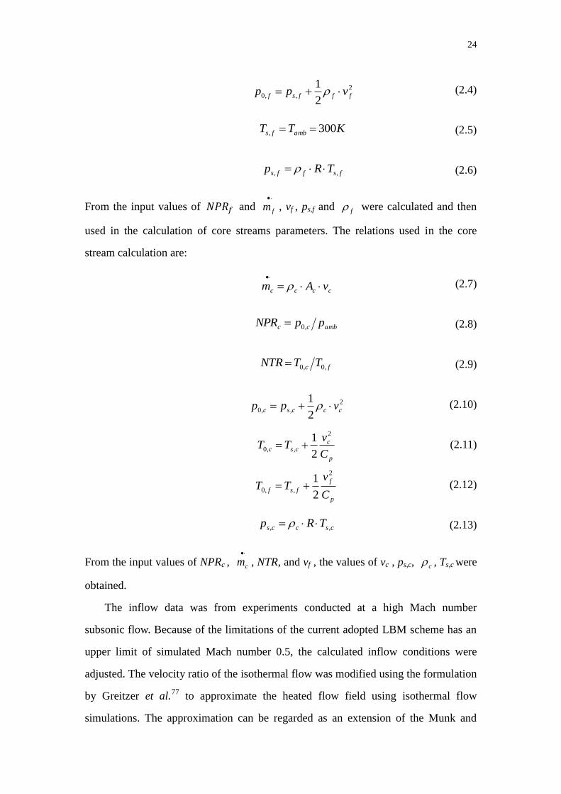
pressure and mean velocity values. The calculation was based on the assumption of an

isentropic flow condition, therefore it is an approximation. The relations used in the

fan stream calculation are as follows:

ffff vAm

(2.2)

ambff ppNPR ,0

(2.3)

24

2

,,02

1fffsf vpp (2.4)

KTT ambfs 300, (2.5)

fsffs TRp ,, (2.6)

From the input values of and

fm , vf , ps,f and f were calculated and then

used in the calculation of core streams parameters. The relations used in the core

stream calculation are:

cccc vAm

(2.7)

ambcc ppNPR ,0 (2.8)

fc TTNTR ,0,0 (2.9)

2

,,02

1cccsc vpp (2.10)

p

ccsc

C

vTT

2

,,02

1 (2.11)

p

f

fsfC

vTT

2

,,02

1 (2.12)

csccs TRp ,, (2.13)

From the input values of NPRc ,

cm , NTR, and vf , the values of vc , ps,c, c , Ts,c were

obtained.

The inflow data was from experiments conducted at a high Mach number

subsonic flow. Because of the limitations of the current adopted LBM scheme has an

upper limit of simulated Mach number 0.5, the calculated inflow conditions were

adjusted. The velocity ratio of the isothermal flow was modified using the formulation

by Greitzer et al.77

to approximate the heated flow field using isothermal flow

simulations. The approximation can be regarded as an extension of the Munk and

25

Prim substitution for steady isentropic flows to non-isentropic flows. The adjusted

operating conditions are listed in Table 2.3. A comparison between the simulated

operating conditions in the current study and the experimental test conditions in

previous studies72

is shown in Table 2.5.

A hyperbolic tangent velocity profile was used to mimic the fully turbulent

velocity profile at the nozzle inlet. The formulation was given by Freund78

:

,tanh12

1)( 0

0

r

r

r

rbvrv

(2.14)

where 22 yxr , r0=1, b is a constant, and v is the mean inlet velocity for fan or

core stream.

In order to match with the actual turbulent intensity level and to perturb the

boundary layer close to the nozzle tip, a forcing procedure76

was followed. The

boundary layer was perturbed close to the nozzle inlet. Random velocity fluctuations

of low amplitude were added in the boundary layer to generate negligible spurious

acoustic waves. These fluctuations were random both in time and space, whereas they

were based on vortical disturbances decorrelated in the azimuthal direction as in LES

schemes. The tripping magnitudes were empirically chosen to obtain, at the nozzle

exit, a turbulence intensity of 5%. In this study, the three forcing velocity components

were applied in the following way:

,

),,,(3

),,,(2

),,,(

tzr

tzr

tzr

v

v

v

v

v

v

v

z

r

j

z

r

z

r

(2.15)

where ),,,( tzrr , ),,,( tzr , and ),,,( tzrz were random numbers between -1

and 1 updated at every time step and at every grid point. =0.00625 was used here

to achieve the desired turbulence intensity level.

26

Mixer ID Lobe Penetration

Hm/Hmp

Scalloping

Depth

Ls/Hm

Area Ratio

Af/Ac

*CONF N/A N/A 2.34

†20UH 0.48 0 2.34

‡20MH 0.48 0.399 2.34

§20DH

**12CL

0.48

0.41

0.686

N/A

2.34

2.34

Table 2.1: Mixer geometric parameters.

*Confluent mixer; †20 lobe unscalloped mixer with high penetration; ‡20 lobe medium scalloped

mixer with high penetration; §20 lobe highly scalloped mixer with high penetration; **12-lobe

unscalloped mixer with low-penetration.

pchar 101,000 Pa

Vchar 67.32 m/s

Tchar 300 K

char 15.75×10-5

m2/s

Lchar 0.1847 m

Re 1.36×106

r 435

Simulated highest Mach number 0.5

(Same as experiment)

ts 1,000,000 time steps

tts 6.918×10-7

s

Turbulent intensity 5%

Turbulent length scale 0.0129 m

(0.07 ×characteristic length)

Table 2.2: Numerical simulation characteristic parameters.

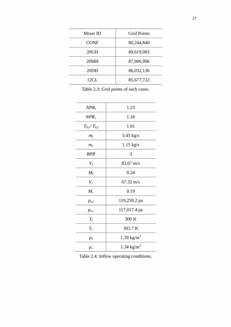
27

Mixer ID Grid Points

CONF 80,244,840

20UH 89,619,083

20MH 87,906,996

20DH 86,032,136

12CL 85,677,722

Table 2.3: Grid points of each cases.

NPRf 1.23

NPRc 1.18

T0,c/ T0,f 1.01

mf 3.45 kg/s

mc 1.15 kg/s

BPR 3

Vf 83.67 m/s

Mf 0.24

Vc 67.32 m/s

Mc 0.19

ps,f 119,259.2 pa

ps,c 117,017.4 pa

Tf 300 K

Tc 303.7 K

f 1.39 kg/m3

c 1.34 kg/m3

Table 2.4: Inflow operating conditions.

28

Mixer

ID

Simulation Operating Condition Experimental Operating Condition

NPRf NPRc T0,c/ T0,f Vf

(m/s)

Vc

(m/s) NPRf NPRc T0,c/ T0,f

Vf

(m/s)

Vc

(m/s)

CONF 1.22 1.18 1.01 83.67 67.32 1.44 1.40 2.34 129.0 148.7

20UH 1.22 1.18 1.01 83.67 67.32 1.44 1.39 2.50 129.0 160.8

20MH 1.22 1.18 1.01 83.67 67.32 1.44 1.39 2.50 129.0 160.8

20DH 1.22 1.18 1.01 83.67 67.32 1.44 1.39 2.50 129.0 160.8

12CL 1.22 1.18 1.01 83.67 67.32 1.44 1.40 2.35 129.0 149.3

Table 2.5: Operating conditions of the current study and previous experiments.

29

Figure 2.1: Schematic of the mixer-nozzle configuration.

Figure 2.2: Sketch of a scalloped mixer.

30

(a) (b)

(c) (d)

(e)

Figure 2.3: Drawings of the five mixer models. (a): CONF; (b): 12CL; (c) 20UH; (d)

20MH; (e) 20DH.

31

Figure 2.4: Streamwise view of the computational domain and VR regions.

Figure 2.5: A different view of the computational domain and VR regions.

32

Figure 2.6: A schematic of the VR regions close to the nozzle.

Figure 2.7: An isometric view of the zoom-in VR regions.

33

Figure 2.8: Streamwise view of voxel distribution in the entire domain.

Figure 2.9: Streamwise view of voxel distribution inside the nozzle.

34

Figure 2.10: An isometric view of voxel distribution near the nozzle.

Figure 2.11: Voxel distribution at the nozzle exit.

35

Figure 2.12: Streamwise measurement window and 3D measurement window. Blue

square box: Streamwise measurement window; red cylinder: 3D measurement

window.

Figure 2.13: Porous FWH control surface.

36

Figure 2.14: Inlet geometries. Blue plate: fan stream inlet; yellow plate: core stream

inlet.

Figure 2.15: Outlet boundary geometry. Red solid plate: outlet.

37

Figure 2.16: Inlet surfaces of the artificial forcing.

38

Chapter 3 Effects of Lobe Number and Penetration Depth

The aerodynamic performance and noise emissions of three unscalloped mixers

(i.e., CONF, 12CL, 20UH) were investigated. With the confluent mixer as a baseline,

the 12CL and 20UH configurations were selected to study the compounded effects of

lobe number and penetration depth. Although the consequences of changes in these

two geometrical parameters are not independent, the effects of increased interface area

between core and fan streams were studied. Instantaneous and time-averaged flow

results and statistics were obtained. Plume survey data revealed the local velocity

distribution across transverse cross-sections of the jet at different downstream

locations to help relate the plume flow physics and the radiated sound. Overall sound

pressure levels (OASPL) and sound pressure level (SPL) directivity results were

obtained for the three mixers. The results qualitatively matched previous experimental

findings.

3.1 Aerodynamic Results and Analysis

The same operating conditions (i.e., velocity and static pressure) were imposed in

the simulation for the three mixer-nozzle configurations. Because the three models

also had the same fan inlet and core inlet area, the bypass ratios (BPR, defined as mf

/mc) were identical. Figure 3.1 shows a snapshot of the transient streamwise velocity

iso-surface (Ux=80 m/s) qualitatively representing the diffusion of momentum in the

quiescent fluid medium interacting with the jet shear layer. Figure 3.2 (a) to (c) shows

the instantaneous total velocity contours of the three mixers. These are within planes

along the jet centerline, through the lobe crests of 12CL and 20UH. The 12CL mixer

had the highest jet exit velocity (i.e., time- and space-averaged velocity magnitude at

the nozzle exit) of 149.65 m/s (Mach 0.43), while the 20UH mixer had the lowest jet

39

velocity of 142.30 m/s (Mach 0.41). It can be observed from Figures 3.1 and 3.2 that

the flow field reached a fully turbulent state within one jet diameter downstream of

the nozzle exit. The turbulent jet cores broke approximately eight jet diameters

downstream of the exit.

Figure 3.3 (a) to (c) shows close-up views of instantaneous vorticity inside the

three nozzles. It can be seen from Figure 3.3 (a) that there was hardly any mixing

between core and fan streams downstream of the confluent mixer. The only turbulent

vortex shedding pattern observed was immediately downstream of the center body

due to flow separation. For the two lobed mixers, Figures 3.3 (b) and (c) show clearly

the mixing phenomenon inside the nozzle. For both the 12CL and the 20UH mixers,

flow separation occurred near the upper wall of the lobe. The vortex shedding process

occurred immediately downstream to the 20UH mixer exit. For the 12CL mixer, there

was no vortex observed until around one lobe height downstream of the mixer exit.

Due to a greater lobe number, the 20UH mixer had smaller lobe widths which were

the characteristic length for the vortex produced by the mixer. Figures 3.3 (b) and (c)

confirm that the 20UH mixer had a much smaller vortex length scale compared to the

12CL mixer. Figures 3.3 (b) and (c) show that the vortex shedding location of 20UH

was much closer to the nozzle wall, and the vortex detached from the 20UH mixer

entered the shear layer downstream of the nozzle exit plane. This can be explained by

the high penetration depth of the 20UH mixer. It can be inferred that increased

turbulent intensity added into the shear layer might increase the far-field noise level.

However, as discussed in section 3.2, it was observed that this penalty is not

significant in comparison with noise reduction benefits of the 20UH mixer.

Figure 3.4 (a) to (c) shows the lambda 2 criterion iso-surface for the three mixers

(iso-surface value = -100). Lambda 2 was defined as the second eigenvalue of the

symmetric tensor S2+Ω

2, where S and Ω were respectively the symmetric and

anti-symmetric parts of the velocity gradient tensor u. This criterion has been shown

to accurately capture vortex structure79

and to properly visualize the 3D turbulent

coherent structures. The 12CL and 20UH mixer featured intensive mixing processes,

40

while the confluent mixer did not produce any significant mixing pattern.

Figures 3.5 (a) to (c) show the mean streamwise velocity contour at the nozzle

exit plane. In terms of magnitude, the 12CL mixer had the highest average and peak

velocities, and the 20UH had the lowest. The confluent mixer had a contour similar to

that of the simple dual stream coaxial jet. The circular ring region of low velocity

magnitude indicated the mixing area where interaction between the two streams

occurred due to Kelvin-Helmholtz instability. The energy loss caused by flow

separation behind the center body led to the velocity deficit visible in the center

region of the contour. As seen from Figures 3.5 (b) and (c), there are clear indications

of the 12CL and 20UH lobe shapes at the exit of the nozzle. The lobed mixers

considerably reduced the velocity within the core region associated with the confluent

mixer. The greater lobe number and deeper penetration caused the 20UH mixer to

exhibit a relatively more uniform flow profile than that of the 12CL.In comparison

with the 12CL mixer, the wetted area of the high velocity region for the 20UH mixer

was smaller and closer to the nozzle wall due to the high penetration length. Because

a more uniform flow velocity profile at the nozzle exit should lead to reduced noise

levels, the OASPL level for the 20UH was expected to be lower than that for 12CL.

Figure 3.6 (a) to (c) shows the time-averaged mean streamwise velocity contour

for the three cases along the jet center plane. Identical to the previous results, for all

three cases, a velocity deficit region extended from the end of the center body to

approximately two diameters downstream of the nozzle exit plane. The confluent

mixer did not show any evidence of significant mixing, and there were velocity peaks

close to the nozzle lip. The 12CL mixer produced a high velocity region close to the

nozzle lip line, which extended from slightly upstream of the nozzle exit to about 1.5

jet diameters downstream of the exit. In contrast to the confluent mixer, the 20UH had

a fairly well mixed flow profile, with high velocity regions confined within the nozzle.

The three mixers produced about the same potential jet core length.

The corrugated azimuthal flow profiles in the lobed mixer cases became smooth

and axisymmetric downstream of the nozzle exit due to the good azimuthal mixing

41

produced by the axial vortices. Hence, a center line velocity decay comparison should

give a fairly good indication of the overall relative noise levels produced by the lobed

mixer. The centerline mean streamwise velocity comparison is shown in Figure 3.7.

The velocities were normalized by the jet velocity, and the measurement started from

the nozzle exit plane. Within the first jet diameter, there were initial increases for all

three cases due to the velocity deficit. From approximately two to six diameters

downstream of the exit, the velocities remained nearly constant, except that inside the

confluent mixer-nozzle the velocity continued to rise gently. Note that the peak

velocity of the confluent mixer was about 10% Uj higher than the 12CL. The next

section looks at whether this would affect the far-field noise level. Further

downstream, the three cases yielded a similar decay rate for the centerline velocity.

Figure 3.8 (a) to (c) shows the mean turbulent kinetic energy contour for the three

cases. The low energy near the nozzle lip indicates a nearly laminar exit shear layer.

Interestingly the flow reached a fully turbulent state, or its peak turbulent kinetic

energy level, at different downstream locations for the three mixers. The peak

turbulent kinetic energy level was reached at around 0.6Dj, 0.5Dj, and 0.4Dj

downstream of nozzle exit plane for the confluent, 12CL, and 20UH mixers

respectively. Lobed mixers are expected to produce higher turbulent energy levels

than the confluent mixer in the shear layer because of enhanced mixing. The 20UH

mixer had turbulent kinetic energy concentrations closer to the nozzle than did the

12CL. The addition of streamwise vorticity into the nozzle exit shear layer clearly

increased mixing, causing the turbulent kinetic energy to peak further upstream.

Figure 3.9 shows non-dimensional centerline mean turbulent kinetic energies as a

functions of streamwise distance. It can be observed that the 12CL and 20UH mixers

reached a peak level further upstream than the confluent mixer. Comparing the two

lobed mixers, it appeared that the 12CL reached the highest turbulent kinetic energy

level earlier than the 20UH. This might be because the high penetration of the 20UH

mixer tended to guide the energy-containing vortices towards the nozzle wall and

away from the nozzle centerline. In terms of magnitude, the value of the confluent

42

mixer was 0.3% higher than that of the 20UH, and 0.5% higher than that of the 12CL.

Further downstream, the turbulent kinetic energy of the 12CL and 20UH mixers

decayed at about the same rate, slightly faster than that of the confluent mixer.

Figure 3.10 (a) to (f) shows cross-stream views of mean streamwise velocity

contours at different streamwise locations. From Figure 3.10 (a), it can be seen that

small-scale vortices started to form at the crest and valley of the lobes of the 12CL

and the 20UH mixers. This observation has been reported previously 5,72

. The velocity

magnitude of the fan and core streams was similar for the 12CL and 20UH mixers,

whereas the two streams surrounding the confluent mixer did not show any sign of

mixing. Viscous mixing in the confluent mixer, the dominant mechanism available,

was obviously not effective. The Kelvin-Helmholtz instability was apparently not a

strong mixing mechanism for the confluent mixer with a fan-to-core velocity ratio of

1.24. From Figure 3.10 (b), at the nozzle exit, clear ‘footprints’ of the lobe shape can

be detected for the 12CL and 20UH mixers. One can qualitatively say the 20UH

mixer was better mixed than the 12CL. The greater penetration and lobe number of

the 20UH mixer increased the interface area between the two streams. Previous

experimental results have indicated that this effect is conducive to faster mixing3. The

enhanced mixing mechanism was largely attributed to the streamwise vorticity

generated by the difference in radial velocity components of the core and fan flows

near each lobe sidewall. The axial vorticity generated downstream of the lobe

sidewalls rotated the two flows around each other in tight spirals, increasing the

interface area, producing better mixing. The effect of lobe penetration on the radial

location of the vortices at the nozzle exit plane was also clearly captured. The 12CL

mixer, with low penetration, had its axial vortices closer to the central axis than 20UH.

Because the nozzle exit radius is smaller than the radial height of the lobe crests in

20UH, it appeared that these axial vortices could be interacting with the nozzle wall at

the very aft end. This was confirmed by results from Figure 3.3 (c). Figure (c) to (f)

shows that after one jet diameter, the lobed pattern started to become diffuse, and then

became axisymmetric further downstream.

43

Figure 3.11 (a) to (c) shows a plume survey of mean streamwise velocity across

transverse cross-sections of the jet at different downstream locations. For all cases, the

initial complicated structure of the velocity profiles gave way to a simpler plume

further downstream. The velocity magnitude continued to increase beyond the exit

until one diameter downstream. High-velocity gradients were observed at the nozzle

lip shear layer. For the confluent mixer, in the region within one diameter from the

exit plane, high-velocity gradients were observed at the radial locations where the two

streams interacted. The velocity deficit also caused high-velocity gradients in the

vicinity of the centerline. As for the 12CL mixer, within one diameter downstream of

the exit, there were high-velocity gradients concentrated close to the inner side of the

nozzle lip line. The velocity deficit effect was decreased due to mixing. It is

interesting to see that for the 20UH mixer the large velocity gradient near the inner

surface of the nozzle lip line was diffused almost immediately downstream of the

nozzle exit, and the velocity profile varied gently further downstream. This should be

attributed to the high penetration depth and enhanced mixing process of the 20UH

mixer. The radial gradients in axial velocity govern part of the turbulence intensity

and are strong sources of noise. The plume generates noise not only from the radial

gradient in velocity at the nozzle-lip shear layer, but also from axial vortex structures

and velocity peaks. These are excess noise sources, in the sense that they do not occur

in a jet with equivalent uniform velocity at the nozzle exit plane. In the next section,

the impact of velocity gradients on the far-field noise was examined.

The mean thrust coefficients of the three cases were compared and listed in Table

3.1. The coefficient was calculated as follows:

Au

FCT

2

2

1

, (3.1)

where

)()( ajj PPAdAnVVF . (3.2)

44

The results showed that the geometric difference of the different lobed mixers didn’t

have a significant impact on the produced mean thrust coefficient.

3.2 Acoustic Results and Analysis

Figures 3.12 to 3.15 show the OASPL directivity and the associated SPL

directivity comparison for the confluent, 12CL, and 20UH mixers. Recall that the

results were obtained for a stationary mean flow with no forward flight effects. The

virtual microphones were located on a circle with a radius of 45m (21Dj), covering the

angles from 45 to 160 degree relative to the nozzle inlet axis.

The OASPL level of the confluent mixer was the highest, as expected. Compared

to the confluent mixer, 12CL had the largest OASPL reduction of 2.7 dB at a

45-degree angle and around 2 dB reduction at aft angles. The 20UH OASPL

directivity followed a trend similar to that of the 12CL mixer, but it had the lowest

OASPL level at all angles. The two lobed mixers both reached a peak level at around

140-degree angle, which is consistent with experimental results72

. The OASPL

directivity of the confluent mixer reached a peak value at 145 degrees, and remained

constant in locations further downstream. The OASPL result further confirmed

experiment results72,73

that the two tested lobed mixers yielded a significant noise

reduction benefit over the confluent mixer. It also indicated that the increased

interface area offered by the 20UH mixer produced additional OASPL reductions

compared to the 12CL mixer.

From Figure 3.13, band-passed SPL directivity at 120 hz, it can be observed that

the confluent mixer was 4 dB higher than the 20UH mixer at most angular locations

and about 5 dB higher than the 12CL mixer at a shallow angle of 160 degrees. All

three mixers reached a peak level at a 160-degree angle. This can be explained by the

fact that the jet plume usually decays far downstream of the nozzle exit, and large

eddies there govern the low frequency domain. This trend was also consistent with

previous experimental results72

. Lobed mixers were expected to do fairly well in

suppressing low frequency noise. The introduction of the lobed mixer was intended to

45

break the large vortices into smaller eddies to reduce the dominant low frequency

noise of the confluent mixer. The 20UH mixer yielded a lower low frequency SPL

level than 12CL at most of the angles. As explained earlier, the lobe width (i.e., the

characteristic length of the vortex produced by the mixer) of 20UH was smaller than

that of 12CL. It seems plausible to relate this fact to the noise suppression at low

frequencies.

Figure 3.14 shows the 1200 hz SPL directivity for the three mixers. The confluent

mixer was not the noisiest mixer in the mid-frequency domain, as found in previous

experiments72,73

. Instead, the 12CL mixer yielded the highest levels at most observer

angles. At locations downstream of 140 degrees, both of the lobed mixers yielded

higher SPL levels than the confluent, as expected. The peak of the lobed mixers’ SPL

level appeared to be shifted with the variation of lobe number and penetration depth.

The 12CL and 20UH mixer had a 3 dB difference in terms of SPL peak value. The

20UH mixer remained quieter than 12CL; however, the advantage of 20UH over

12CL in suppressing mid-frequency noise was not as significant as in the low

frequency domain. The results indicate that the dominant contribution to the overall

mid-frequency noise of lobed mixers was from the downstream angles between 135

and 150 degrees.

The SPL directivity comparison at 4500 hz is shown in Figure 3.15. Except at

locations of 85 to 125 degree angles, the high frequency SPL level for the confluent

mixer was mostly lower than for the 12CL and 20UH mixers. At positions

downstream of the 140-degree angles, the 12CL mixer was quieter than 20UH, and a

reduction of 4 dB at a 160-degree angle was obtained. The overall high frequency SPL

trends of 12CL and 20UH were similar, and the magnitude was comparable. The

20UH mixer did not seem to produce a significant increase in the high frequency

range while suppressing low-to-mid frequency noise. Note that the peak SPL value for

12CL and 20UH was reached at 125- and 135-degree angles respectively. In

comparison with the SPL trends over the mid-frequency range, the peak angles were

reached further upstream because high frequency noise is usually attributable to

46

smaller eddies which predominate near the nozzle exit plane or even inside the nozzle,

according to turbulent jet theory80

. High frequency noise is more likely to concentrate

at upstream locations81

.

Considering the overall trends for the three mixers, the large reduction in

low-frequency noise was found to lead to a lower OASPL level for the two lobed

mixers. In the mid-to-high frequency domain, the confluent mixer was mostly quieter

than 12CL and 20UH. The 12CL mixer had higher low-to-mid frequency noise and

lower high frequency SPL level in the far downstream than 20UH. The high

penetration depth and greater lobe number of 20UH brought the extra benefit of

decreasing mid-frequency noise while maintaining considerable reduction in

low-frequency noise.

3.3 Summary

Inside the 20UH mixer-nozzle were small-scale vortices shed from the mixer tip

which entered the downstream nozzle lip shear layer. This effect, however, did not

increase the turbulent kinetic energy significantly. The data showed that the peak

value of turbulent kinetic energy along the nozzle lip-line was lower downstream of

the 20UH mixer-nozzle than for the 12CL. Figure 3.15 shows that the far-field

high-frequency noise level of 20UH remained comparable to that of the 12CL.

Although the high penetration tended to guide the vortices towards the nozzle wall

and the downstream shear layer, this factor did not seem to increase far-field sound.

The uniformity of the velocity profile at the nozzle exit may be indicative of the

differences in the three mixers’ OASPL level. The 20UH mixer had the most uniform

exit velocity profile, followed by the 12CL and confluent mixer. From Figure 3.12, it

was found that 20UH had the lowest OASPL level. The decreased high velocity

gradient of 20UH as seen in Figure 3.11 (c) provided a possible explanation for the

low high-frequency SPL level of 20UH. The high velocity gradient near the jet center

line downstream to the confluent mixer might explain why it had a relatively higher

SPL level in the high-frequency domain (see Figure 3.15).

47

For a simple round jet, a correlation exists between the downstream mean

centerline velocity decay rate and the far-field low frequency noise level72

. A faster

decay rate usually results in reduced low frequency noise level. However, from

Figures 3.7 and 3.13, it is hard to determine whether there was a direct relation

between the two factors for jet flow exited from lobed mixers.

Figure 3.8 (a) to (c) showed that the turbulent kinetic energy of the 20UH mixer

peaked downstream those of the 12CL and confluent mixer. Calculations showed,

however, that the peak turbulent kinetic energy value along the 20UH nozzle lip line

was lower than that of 12CL. On the other hand, the OASPL level in Figure 3.12

shows that 20UH had the lowest OASPL level. Therefore, for lobed mixers, it is

plausible that it should be the magnitude of the turbulent kinetic energy inside the

nozzle lip shear layer that determined the far-field sound level, rather than the

increasing rate of the turbulent kinetic energy.

Finally, the overall effect of increasing lobe number and penetration depth

increases the interface area between the fan and the core flows and decreases the

length scale of the axial vortices. This should enhance mixing between the two flows.

A decrease in the length scale of the axial vortices seems to imply an increase in the

dominant frequency, but it is true only if their strengths remained the same. As the

lobe number and penetration depth increase, the number of vortices occupying the

space within the nozzle must also increase. This promotes upstream azimuthal

interaction between the vortices and reduces their strength. It has been shown from

Figure 3.14 that the mid-to-high frequency sound of 12CL and 20UH was associated

with these axial vortices. In Figure 3.12, the mid-frequency content of the 20UH

mixer was less than that of the comparable 12CL mixer. This seemed to imply that an

increase in the lobe count produced a reduction in the strength of the axial vortices

due to better azimuthal mixing of the axial vortices. On the other hand, the 20-lobe

mixer, 20UH, was also effective in reducing the low frequency portion of the

spectrum which was typically related with the far downstream plume characteristics.

Penetration played a role in the radial migration of the axial vortices generated by the

48

mixers. This change in radial migration determined whether the vortices would

interact with the outer nozzle wall and modify the ambient-jet shear layer. The12CL

low-penetration mixer kept the axial vortices closer to the jet centerline. This should,

to some extent, prevent the core flow from immediately interacting with the ambient

shear layer, and hence reduce the mid-to-high frequency noise from that region.

However, these vortices could modify the flow further downstream and change the

noise characteristics in a different manner which might be why (shown in Figure 3.15)

substantial reduction was not obtained in the high-frequency domain.

49

Mixer ID Ts,c/Ts,f Mj CT

Confluent 1.0 0.41 1.95

12CL 1.0 0.42 1.94

20UH 1.0 0.43 1.94

Table 3.1: Mean thrust coefficient comparison between the three tested cases.

50

Figure 3.1: Transient streamwise velocity iso-surface (Ux=80 m/s).

(a)

(b)

51

(c)

Figure 3.2: Instantaneous total velocity contours of the three mixers. (a): confluent

mixer; (b): 12CL; (c): 20UH.

(a)

52

(b)

(c)

Figure 3.3: Close-up view of instantaneous vorticity inside the three nozzles. (a):

confluent mixer; (b): 12CL; (c): 20UH.

53

(a)

(b)

54

(c)

Figure 3.4: Lambda 2 criterion iso-surface for the three mixers. (a): confluent mixer;

(b): 12CL; (c): 20UH. (iso-surface value = -100)

(a)

55

(b)

(c)

(m/s)

Figure 3.5: Mean streamwise velocity 3D contour at the nozzle exit plane. (a):

confluent mixer; (b): 12CL; (c): 20UH.

56

(a)

(b)

(c)

Figure 3.6: Time-averaged mean streamwise velocity contour for the three cases along

jet center plane. (a): confluent mixer; (b): 12CL; (c): 20UH.

57

Figure 3.7: Center-line mean streamwise velocity. Blue line: confluent mixer; green

line: 12CL; red line: 20UH.

(a)

(b)

58

(c)

Figure 3.8: Time-averaged mean turbulent kinetic energy contour. (a): confluent mixer;

(b): 12CL; (c): 20UH.

Figure 3.9: Non-dimensional center-line mean turbulent kinetic energy. Blue line:

confluent mixer; green line: 12CL; red line: 20UH.

59

(a)

(b)

(c)

(d)

60

(e)

(f)

Figure 3.10: Transwise views of mean streamwise velocity contour at different

streamwise locations. From left to right: confluent mixer, 12CL, 20UH; (a): at mixer

exit plane; (b): at nozzle exit plane; (c): 1Dj downstream of the nozzle exit; (d): 2Dj

downstream of the nozzle exit; (e): 3Dj downstream of the nozzle exit; (f): 4Dj

downstream of the nozzle exit.

61

(a)

(b)

62

(c)

Figure 3.11: Downstream plume survey of mean streamwise velocity across

transverse cross-section of the jet at different downstream locations. (a): confluent

mixer; (b): 12CL; (c): 20UH. Dark blue line: at nozzle exit plane; green line: 0.2Dj

downstream of the nozzle exit; red line: 0.5Dj downstream of the nozzle exit; light

blue line: 1Dj downstream of the nozzle exit; purple line: 3Dj downstream of the

nozzle exit; brown line: 5Dj downstream of the nozzle exit.

63

Figure 3.12: OASPL directivity. : confluent mixer; : 12CL; : 20UH.

Figure 3.13: Band-passed 120hz SPL directivity. : confluent mixer; : 12CL;

: 20UH.

64

Figure 3.14: Band-passed 1200hz SPL directivity. : confluent mixer; : 12CL;

: 20UH.

Figure 3.15: Band-passed 4500hz SPL directivity. : confluent mixer; : 12CL;

: 20UH.

65

Chapter 4 Effects of Scalloping

In this chapter, effects of scalloping of the lobe mixers are discussed. A group of

three 20-lobe high-penetration mixers with various scalloping depth was investigated.

The confluent mixer was chosen as the baseline. Instantaneous and time-averaged

flow results and statistics were obtained. Plume survey data is shown in terms of local

velocity distribution across transverse cross-sections of the jet at different downstream

locations. Overall sound pressure level (OASPL) and sound pressure level (SPL)

directivity results are also reported for the four mixers to characterize the far-field

radiated noise. The results are in qualitative agreement with experimental data.

4.1 Aerodynamic Results and Analysis

The same operating conditions (i.e., velocity and static pressure) were imposed in

the simulation for the four mixer-nozzle configurations. All four models had the same

fan inlet and core inlet area, therefore the bypass ratios were also the same. Figure 4.1

(a) to (c) shows instantaneous streamwise velocity contours for the four cases. These

are slices along the jet centerline, through the lobe crests. The exit jet velocities for

the three 20-lobe mixers were almost the same, at around 141m/s (Mach 0.406), while

the confluent mixer had an exit jet velocity of 142.5 m/s (Mach 0.411). Transition

from laminar to turbulent for the three lobed mixers occurred upstream of confluent

mixer. The 20UH and 20DH mixers turned fully turbulent at around 0.8 Dj

downstream of the nozzle exit, while 20MH underwent transition at around 0.4 Dj.

This quantitative difference should result in differences between turbulent kinetic

energy levels and far-field sound pressure levels. Whether or not the 20MH mixer is

distinct from the other two lobed mixers is examined in the next sections. Because the

potential jet core length is often used as an indicator of noise level, the values for the

66

four cases are compared. The length of the potential core is defined here as the

distance over which the jet centerline velocity is reduced to 95% of its peak value,

Ucenterilne(xcenterline) = 0.95Upeak. The values of the potential core lengths are listed in

Table 4.1. Note that as scalloping depth increased, the potential core length decreased.

The jet core length of 20DH was 8.7% shorter than that of the 20UH mixer.

Figures 4.2 (a) to (d) show close-up views of the instantaneous vorticity inside the

four nozzles. In comparison with lobed mixers, the confluent mixer does not exhibit

significant mixing between core and fan streams. In contrast, the three lobed mixers

do exhibit extensive mixing inside the nozzle. Flow separation along the lobe crest is

observed, due to the high penetration depth. Vortices are initiated and shed from the

lobe almost immediately downstream of the mixer exit. These vortices are then

convected over the nozzle lip shear layer, increasing the turbulent intensity level.

Because scalloping led to upstream mixing and interaction between the two streams,

the lobe width may not constitute an appropriate characteristic length for the

streamwise vortices. There are some differences, therefore, between the vortex

shedding patterns of the three lobed mixers. Increased dissipation occurred

downstream of the mixer exit as the scalloping depth was increased. In contrast to

20UH, the 20DH mixer produced more small-scale vortices. This is because the

distance over which mixing occurs for 20DH is greater than for the 20UH. At the

mixer exit plane, 20DH is already partially mixed while the 20UH mixer is only

slightly beyond mixing initiation. It was mentioned in the last chapter that a high

penetration depth, or lobe height, tends to lead the shed vortices towards the nozzle

wall and away from the jet center line. It is interesting to see here that the path of the

two scalloped mixers vortices is directed towards the jet flow central region

interacting with the flow further downstream. This implies that the introduction of

scalloping produced an effective lobe penetration that is no longer characterized by

the lobe height only. Both the scalloping depth and the lobe height should be taken

into account for a better characterization of the vortex-affected area.

Lambda 2 criterion iso-surface was shown in Figure 4.3 (a) to (d). Mixing was

67

initiated along the scalloping profile in the two scalloped mixers. The mixing for the

20MH and 20DH cases, indeed, started earlier than that for the 20UH unscalloped

mixer.

Figure 4.4 (a) to (d) shows the 3D mean streamwise velocity contour at the nozzle

exit plane. The three lobed mixers had more uniform velocity profiles than the

confluent mixer. Furthermore, the two scalloped mixers had more uniformity than the

20UH mixer. The 20DH mixer seemed to have a better mixed flow profile than 20MH.

The clear ‘footprint’ of the lobe in 20UH was not seen in 20MH or 20DH.

Qualitatively, the high velocity gradient region was closer to the nozzle wall in the

scalloped mixers. The energy loss caused by flow separation behind the center body

led to the velocity deficit in the center region of the contour.

Figure 4.5 (a) to (d) shows the time-averaged mean streamwise velocity contours

both inside and outside the nozzle. There were velocity ‘hot spots’ at the nozzle exit

wall for all the cases. The 20DH mixer appeared to have a more uniform velocity

profile from the nozzle exit to several jet diameters downstream. It has been said that

the design philosophy behind scalloping is to introduce axial vorticity gradually into

the flow so that fan and core stream mixing can proceed more gradually than in the

unscalloped mixer. The most intense turbulence spots are then acoustically shielded

by the nozzle duct. This does not necessarily lead to a more uniform velocity profile

by the time the two streams reach the nozzle exit plane; however, it tends to reduce

the mid-to-high frequency noise generated by internal mixing and by the interaction

of the partially mixed flow with the ambient.

A centerline mean streamwise velocity comparison is shown in Figure 4.6. Within

the first jet diameter downstream of the nozzle exit, all four cases experienced a rapid

increase and reached a relatively stable stage, until the values started to decay at

around six jet diameters. The 20UH and 20MH mixers reached a peak value upstream

of the confluent mixer, and there was no significant difference between these two

cases. The 20DH mixer is distinct from the other two lobe mixers. It featured a steady

velocity increase from the nozzle exit to four diameters downstream. Its peak value

68

was nearly the same as that of the confluent mixer. The magnitude was 7% larger than

that of the 20UH mixer. This might be attributed to the interaction between the

vortices shed from the 20DH mixer and the downstream jet flow, as shown in Figure

4.2 (d). The 20MH mixer also featured a similar vortex shedding pattern. A more

plausible explanation needs to be found to clarify this phenomenon. The impact on the

far-field sound level is discussed in the next section. Further downstream, beyond ten

jet diameters, all the cases exhibited a similar decay rate.

Figure 4.7 (a) to (d) shows the time-averaged mean turbulent kinetic energy

contours for the four mixers. The low energy level close to the nozzle exit indicated a

nearly laminar exit shear layer. A difference between the turbulent kinetic energy

concentration location was observed among the four cases. The fully turbulent state

was reached at around 0.6Dj, 0.4Dj, 0.2Dj, and 0.5Dj downstream to the nozzle exit

plane for confluent, 20UH, 20MH, and 20DH mixers respectively. The lobed mixers

turbulent kinetic energy was concentrated closer to the nozzle than for the confluent

mixer, as expected. The increase in scalloping depth did not lead to a monotonic

variation of the downstream peak locations. As illustrated in Figure 4.1, the 20MH

mixer flow transition is upstream to that of the other cases. For all three mixer-nozzles,

vortices shed from the mixer tips were convected into the nozzle lip shear layer. The

strengths of the vortices in the three mixers were different. It is reasonable to infer

that the medium scalloping depth of 20MH allowed proper vortex growth producing

the strongest vortices near the nozzle wall. In comparison, 20UH only started to form

vortices after the mixer exit, and the distance over which the vortices developed might

not be long enough. On the other hand, vortices inside the 20DH mixer were formed

much earlier, but by the time those vortices entered the downstream shear layer they

were already partially dissipated. The peak turbulent kinetic energy magnitude of

20MH along the nozzle lip line was 18% higher than those of 20UH and 20DH.

Figure 4.8 presents the normalized centerline mean turbulent kinetic energy

variation along the downstream direction. The confluent mixer produced the highest

turbulent kinetic energy level among the four cases. The turbulent kinetic energy level

69

of the three lobed mixers reached a peak value at approximately the same location,

nine jet diameters downstream of the nozzle exit. The two scalloped lobed mixers had

relatively higher levels than 20UH. This confirmed the previous presumption that the

vortices shed from the scalloped mixer interacted with the jet flow near the centerline

region, and modified the downstream flow development.

Figure 4.9 (a) to (f) shows the mean streamwise velocity contour at different

streamwise locations downstream of the exit. As seen in Figure 4.9 (a), small-scale

vortices were found at the crest and valley of the lobes. The 20MH mixer had larger

and stronger vortices than the other two in the lobe valleys. This fact can be explained

using the previous reasoning: the 20MH mixer offered the appropriate distance for

vortex development and strengthening; 20UH started to form vortices at a later stage,

and hence did not evolve over a long enough distance to acquire sufficient energy;

although the vortices inside the 20DH mixer were formed and shed earlier, they were

dissipated to some extent when they reached the downstream shear layer. From Figure

4.9 (b), it is evident that the 20MH and 20DH mixers did not preserve the lobe shape

‘foot print’ at the exit. Due to the same lobe penetration, the axial vortices had

approximately similar radial locations for the three lobed mixers. The 20MH and

20DH mixers appeared to yield more uniform profiles at the nozzle exit. Beyond one

jet diameter, the growth of the shear layer thickness began to diffuse the lobe pattern,

as shown in Figure 4.9 (c) to (f). The transwise velocity contours tend to be

axisymmetric further downstream.

Figure 4.10 (a) to (d) shows a plume survey of the mean streamwise velocity

across transverse cross-sections of the jet at different downstream locations. For all

cases, the initially complex velocity profile gave way to a simpler plume profile

further downstream. Velocity deficits caused velocity gradients in the vicinity of the

jet center line. High velocity gradients existed for all the mixers, from the nozzle exit

to one diameter downstream. It appeared that the high velocity gradient of the 20MH

mixer started to decrease earlier than the others.

In Table 4.2, the comparison of the mean thrust coefficients between the four

70

cases were made. The values were found to be close to each other.

4.2 Acoustic Results and Analysis

Figures 4.11 to 4.14 show the OASPL directivity and the associated SPL

spectrum for the confluent, 20UH, 20MH, and 20DH mixers. Recall that the results

were obtained for a stationary medium. The fixed virtual probes were located along a

circle with a radius of 45m (21Dj), covering the angles from 45 to 160 degree relative

to the nozzle inlet axis.

The OASPL level of the confluent mixer was again the highest. Among the three

20-lobe mixers, 20MH was the loudest and 20DH was the quietest. Previous

experimental results indicate that the effect of the scalloping depth on the far-field

sound pressure level does not obey a linear relation72

. Aerodynamic results from

Figures 4.1 and 4.7 confirmed this notion. The three mixers had a similar OASPL

trend. The OASPL level of the 20DH mixer was on average 2 dB lower than 20MH,

and 1 dB lower than 20UH. The largest reduction of 4 dB was obtained at 45 and 160

degrees, when comparing confluent and 20DH OASPL levels. The peak magnitude

was reached at a 140-degree angle for the lobed mixers. There was a scalloping depth

threshold to determine whether scalloping would bring noise reduction benefit or

penalty. The medium scalloping of 20MH seemed to be below that value. The deep

scalloping of the 20DH mixer, on the other hand, was over that threshold and brought

the expected noise reduction benefit.

Some interesting points arise when looking at the SPL directivity at 120 hz in

Figure 4.12. The magnitude of all mixers’ SPL level peaked at the 160 degree angle.

This is because the jet plume decayed far downstream of the nozzle exit, where large

eddies governed the low frequency domain. The 20UH mixer had the lowest level of

all, almost 4 dB lower than the confluent and 20MH mixer at shallow angles.

Surprisingly, the 20MH mixer emissions were similar to those for the confluent mixer

at locations downstream of 145 degrees. 20 DH did not yield significant suppression

of low frequency noise, as indicated by experimental results72,73

. The introduction of

71

scalloping did not yield the same low-frequency noise reduction advantage as the

20UH unscalloped mixer, although the scalloped mixers provided reduction benefits

in the low-frequency domain. Because of scalloping and the fact that the vortex length

was not characterized by the lobe width, the development and size of the shed vortex

were changed. This impact can be brought to the further downstream jet flow to

modify the low-frequency noise radiation mechanism, as indicated in Figure 4.2 (c)

and (d). The relatively high low-frequency level partly explained the higher OASPL

level of 20MH.

Figure 4.13 shows the 1200 hz SPL directivity comparison among the three

mixers. As with the experimental results72

, the confluent mixer had lower a

mid-frequency sound pressure level than lobed mixers. 20MH had the highest SPL

level among the four cases at angles upstream of 115 degrees. 20MH was the quietest

mixer downstream of 135 degrees. The 20DH mixer had a higher mid-frequency level

than confluent and 20UH at angles between 45 and 90 degrees. Now recall that the

20MH mixer had the highest peak turbulent kinetic energy level in the nozzle shear

layer. It also had the turbulent kinetic energy concentration region closest to the

nozzle exit. Turbulent kinetic energy in the shear layer is a major contributor to the

mid-to-high frequency noise, and mid-to-high frequency noise is generally located

near the nozzle exit81

. This can explain why at angles of 45 to 125 degrees 20MH had

higher mid-frequency noise level. This should also be the case in the high-frequency

domain. Noise from the three lobed mixers peaked at different locations: 150 degrees,

120 degrees, and 140 degrees for the 20UH, 20MH, and 20DH mixers respectively.

There was clearly a correlation between the scalloping depth and the peak angle, but

further investigation is beyond the scope of the current study.

The SPL directivity comparison at 4500 hz is shown in Figure 4.14. Upstream of

125 degrees, 20MH had the highest high-frequency SPL level among the lobed mixers,

as mentioned earlier. Downstream of 125 degrees, the 20UH mixer produced higher

levels than the others, while the 20MH and 20DH mixers shared a similar SPL trend

and magnitude. From 85- to 125-degree angles there was an SPL variation associated

72

with the scalloping depth. In that range, 20DH had the lowest level. Combining

Figures 4.12 and 4.14, it appears that scalloping tended to trade part of the advantage

of suppressing low-frequency noise for decreasing the noise in the high-frequency

domain. The 20UH, 20MH, and 20DH mixers peaked at 135 degrees, 115 degrees,

and 120 degrees respectively. In addition to a peak shift due to the geometry

difference, there was also an upstream peak shift related to an increase in frequency

domain for the three cases. That is presumably because high frequency noise near the

nozzle exit plane or inside the nozzle may have been emitted to upstream locations.

In summary, all three lobed mixers were quieter than the confluent mixer. There

seemed to be a threshold that determined the benefit or penalty scalloping could bring

to noise reduction. In terms of OASPL and SPL directivity, 20MH distinguished itself

from the other two mixers because of its high turbulent kinetic energy concentration

near the nozzle exit. It was the significant suppression of 20UH in the low-frequency

domain that made it the second quietest mixer. The improved reduction in the

high-frequency domain of the 20DH mixer led to the lowest OASPL level of the

mixers tested. Finally, the peak angles of the three mixers’ SPL level were found to be

shifted upstream when the investigated frequency was increased.

4.3 Summary

As in the Fisher et al.82

coaxial jet model, there appears to be at least two

dominant regions of frequency in lobed mixers. One is the low-frequency peak

governed by the fully mixed region far downstream and the other is the mid-to-high

frequency peak governed by the shear layer between the ambient and the partially

mixed fan-core flow close to nozzle exit. The geometry of the lobed mixer and

changes to the mixing process can be used beneficially to control one or the other of

these peaks. The unscalloped 20UH mixer produced a substantial reduction in

low-frequency noise compared to the confluent design, but an increase in the

mid-to-high frequency domain at angles downstream to 140 degrees was also

observed. The presence of sidewall scalloping maintained the low frequency

73

suppression, although not as much as for the 20UH mixer, and reduced the

mid-to-high frequency penalty.

The unique turbulent kinetic energy distribution of the 20MH mixer led to its

differentiation from the other two lobed mixers in terms of OASPL and SPL levels.

The higher turbulent kinetic energy in the shear layer apparently increased the 20MH

mixer’s noise level in the mid-to-high frequency domain, as reflected in Figures 4.13

and 4.14. The 20DH mixer, however, was able to suppress the mid-to-high frequency

noise to some extent. On the other hand, it has been shown that in the 20MH and

20DH mixers, there were vortices going towards the flow downstream to the center

body and interacting with jet flow. The effect of this was seen in the low frequency

SPL directivity. Both the 20MH and 20DH mixers had higher levels than 20UH in the

low frequency domain. Finally, the higher velocity peak for 20DH at five diameters

downstream to the nozzle exit plane, as shown in Figure 4.6, did not seem to produce

measurable consequence in the far-field sound pressure level.

74

Mixer ID CONF 20UH 20MH 20DH

xcenterline /Dj 8.33 8.36 8.19 7.69

Table 4.1: Potential core length for the four tested cases.

Mixer ID Ts,c/Ts,f Mj CT

Confluent 1.0 0.41 1.95

20UH 1.0 0.43 1.94

20MH 1.0 0.42 1.94

20DH 1.0 0.41 1.93

Table 4.2: Mean thrust coefficient comparison between the four tested cases.

75

(a)

(b)

(c)

(d)

Figure 4.1: Instantaneous total velocity contours of the four mixers. (a): confluent

mixer; (b): 20UH; (c): 20MH; (d): 20DH.

76

(a)

(b)

(c)

77

(d)

Figure 4.2: Close-up view of instantaneous vorticity inside the four nozzles. (a):

confluent mixer; (b): 20UH; (c): 20MH; (d): 20DH.

(a)

78

(b)

(c)

(d)

Figure 4.3: Lambda 2 criterion iso-surface for the four mixers. (a): confluent mixer;

(b): 20UH; (c): 20MH; (d): 20DH. (iso-surface value = -100)

79

(a)

(b)

80

(c)

(d)

(m/s)

Figure 4.4: Mean streamwise velocity 3D contour at the nozzle exit plane. (a):

confluent mixer; (b): 20UH; (c): 20MH; (d): 20DH.

81

(a)

(b)

(c)

(d)

Figure 4.5: Time-averaged mean streamwise velocity contour for the four cases along

jet center plane. (a): confluent mixer; (b): 20UH; (c): 20MH; (d): 20DH.

82

Figure 4.6: Center-line mean streamwise velocity. Dark blue line: confluent mixer;

green line: 20UH; red line: 20MH; light blue line: 20DH.

(a)

(b)

83

(c)

(d)

Figure 4.7: Time-averaged mean turbulent kinetic energy contour. (a): confluent mixer;

(b): 20UH; (c): 20MH; (d): 20DH.

84

Figure 4.8: Non-dimensional center-line mean turbulent kinetic energy. Dark blue line:

confluent mixer; green line: 20UH; red line: 20MH; light blue line: 20DH.

85

(a)

(b)

(c)

(d)

86

(e)

(f)

Figure 4.9: Transwise views of mean streamwise velocity contour at different

streamwise locations. From left to right: 20UH, 20MH, 20DH; (a): at mixer exit plane;

(b): at nozzle exit plane; (c): 1Dj downstream of the nozzle exit; (d): 2Dj downstream

of the nozzle exit; (e): 3Dj downstream of the nozzle exit; (f): 4Dj downstream of the

nozzle exit.

87

(a)

(b)

88

(c)

(d)

Figure 4.10: Downstream plume survey of mean streamwise velocity across

transverse cross-section of the jet at different downstream locations. (a): confluent

mixer; (b): 20UH; (c): 20MH; (d): 20DH. Dark blue line: at nozzle exit plane; green

line: 0.2Dj downstream of the nozzle exit; red line: 0.5Dj downstream of the nozzle

exit; light blue line: 1Dj downstream of the nozzle exit; purple line: 3Dj downstream

of the nozzle exit; brown line: 5Dj downstream of the nozzle exit.

89

Figure 4.11: OASPL directivity. : confluent mixer; : 20UH; : 20MH; :

20DH.

Figure 4.12: Band-passed 120hz SPL directivity. : confluent mixer; : 20UH;

: 20MH; : 20DH.

90

Figure 4.13: Band-passed 1200hz SPL directivity. : confluent mixer; : 20UH;

: 20MH; : 20DH.

Figure 4.14: Band-passed 4500hz SPL directivity. : confluent mixer; : 20UH;

: 20MH; : 20DH.

91

Chapter 5 Conclusions and Future Work

5.1 Conclusions

Four lobed mixers and one baseline confluent mixer were investigated in a

computational study of the aerodynamic and aeroacoustic effects of actual turbo-fan

jet engine mixer-nozzle geometries. The Lattice Boltzmann Method (LBM) was used

because of its advantages to handle complex geometries in the computational domain.

The grid distribution and measurement settings were refined to capture the sensitivity

of the near-field flow patterns and far-field sound levels to the mixer geometric

difference, as was shown by the aerodynamic and acoustic results. The data showed

that the boundary conditions and artificial forcing functions imposed at the inlet

produced realistic turbulent kinetic energy levels downstream of the nozzle exit.

5.1.1 Effects of Lobe Number and Penetration Depth

The first group of mixers was studied to understand the effects of different lobe

number and penetration depth. As expected, lobed mixers enhanced mixing inside the

nozzle relative to the baseline confluent mixer. Results showed that the three mixers

(i.e., confluent, 12CL and 20UH) reached a fully turbulent state within one jet

diameter downstream of the nozzle. Due to a smaller lobe number, the scale of the

vortices shed from the 12CL mixer was found to be larger than from the 20UH mixer.

This may have led to the greater levels of noise in the low-to-mid frequency domain

for the 12CL mixer. The high penetration of 20UH guided part of the vortex into the

shear layer, and, as a consequence, the turbulent kinetic energy level was raised in the

downstream shear layer. The 20UH mixer features a turbulent kinetic energy

concentration at the nozzle exit. However, this did not seem to result in a considerable

92

increase in mid-to-high frequency noise and Overall Sound Pressure Level (OASPL).

The velocity exit profile of 20UH was found to be more uniform than that of 12CL.

The high velocity gradient of 20UH was also smaller and decayed faster than that of

12CL. These two differences were attributed to the increased interface area of the

20UH mixer. There were some differences in mean streamwise centerline velocity

decay pattern, but it did not seem to affect the far-field sound levels.

The two lobed mixers showed their noise reduction benefit over the confluent

mixer. The 20UH mixer demonstrated its capacity for greater noise reduction

compared with 12CL. The smaller scale vortex of 20UH did lead to an improvement

over 12CL in the low-frequency domain. At high frequencies, the noise reduction

advantage of 20UH was not as significant. The 12CL mixer had higher low-to-mid

frequency noise and a lower high frequency SPL level in the far downstream than

20UH. The high penetration depth and higher lobe number of 20UH had the benefit of

decreasing the mid-frequency noise while maintaining considerable reduction in

low-frequency noise. In addition, the results implied an upstream shift in the SPL

level peaks with the frequency increase for all the mixers.

5.1.2 Effects of Scalloping

The 20UH, 20MH and 20DH mixers along with confluent mixer were studied to

uncover the impact of scalloping. The medium scalloping brought the 20MH mixer

the earliest transition to a fully turbulent state and the fastest turbulent kinetic energy

increasing rate among the three lobed mixers. This directly led to the differentiation of

20MH from the other two lobed mixers in far-field sound field. The results suggested

that there might exist a threshold value that determines whether or not scalloping

could yield noise reduction benefits. Because of the different sidewall scalloping, the

characteristic length and strength of the shed vortex in the three mixers were different.

Some vorticity dissipation existed downstream of the scalloped mixers exit. This

impact was reflected in the differences in turbulent kinetic energy levels in the shear

layer, and hence on the far-field SPL directivity level. Scalloping tended to guide the

93

shed vortices towards the central jet flow region thus interacting with the flow further

downstream. All three scalloped mixers had a fairly uniform velocity profile at the

exit, and the high velocity gradient was found close to the nozzle exit wall. The 20DH

mixer had a high peak value of the centerline mean streamwise velocity variation;

however, this did not produce an increase in the far-field sound pressure level.

Among the three mixers, 20DH had the lowest OASPL level, and 20MH had the

highest. The introduction of scalloping did not yield the same low-frequency noise

reduction advantage as for the 20UH unscalloped mixer, but it yielded reduction

benefits in the low-frequency domain. The 20DH results showed that deep scalloping

tended to trade some of the advantage of suppressing low-frequency noise for

decreasing the noise in the high-frequency domain. The SPL directivity showed that

there was a peak shift associated with the scalloping depth variation. The SPL levels

also confirmed an upstream peak shift related to the frequency domain for the three

cases.

5.2 Plans for Future Work

5.2.1 High Mach Number Simulations

Due to the current limit of simulated Mach of LBM, the exit flow velocity was

relatively low compared to practical commercial jet engine operating conditions. A

high Mach version of the LBM-based commercial code is expected to be released for

validation and practice in the near future. By then, the same experimental conditions

of lobed mixers will be utilized in the simulation to achieve the exit jet Mach number

close to 0.9.

5.2.2 Heated Jet Simulation

The current LBM model only allows heated jet simulation with a limit of Mach

0.2. This is apparently not of much practical use for jet noise prediction. With the

release of the high Mach LBM code, high Mach heated jet simulation will be carried

94

out with a fully coupled LBM-heat transfer scheme.

5.2.3 Two-Step Simulation

Jet flow simulation can be divided into internal and external flow simulation.

Depending on whether the simulation domain is inside or outside of the nozzle, the

flow is called internal or external flow. The idea of two-step simulation is to first run

the internal simulation and record all the interested data (i.e., velocity, pressure and

temperature). The recorded data is then fed to the second-step external simulation.

The advantage of this approach is that considerable computational cost is saved

because the expensive second-step external simulation does not need to be started

until the internal flow reaches the fully convergent state. The difficulties are to impose

the proper outlet boundary condition in the first step and reduce the size of the

recorded data. Preliminary study on the confluent mixer has already been conducted,

and it proved technically feasible at the current stage.

5.2.4 Parametric Studies of the Lobed Mixer Geometry

The key parameters of a lobed mixer include lobe number, penetration depth,

scalloping shape, lobe width, lobe height and sidewall cut-off angle. In this study, the

investigation of the scalloping effect can be considered a first step. Because a

systematic experimental study on these parameters is practically almost impossible,

the LBM-based simulation tailored particularly for the complex flow appears to be an

excellent option.

95

References

[1] Hygge, S., Evans, G.W., and Bullinger, M., “A Prospective Study of Some

Effects of Aircraft Noise on Cognitive Performance in Schoolchildren,”

Psychological Science, Vol. 13, No. 5, September 2002, pp. 469–474.

[2] “AeroAcoustics Research Consortium,” (http://www.oai.org/aeroacoustic

/challenge.html).

[3] McCormick, D. C., and Bennett, J. C., Jr., "Vortical and Turbulent Structure of

a Lobed Mixer Free Shear Layer," AIAA Journal, Vol. 32, No. 9, 1994, pp.

1852-1859.

[4] Belovich, V. M., Samimy, M., and Reeder, M. F., "Dual Stream Axisymmetric

Mixing in the Presence of Axial Vorticity," AIAA-94-3084, 30th

AIAA/ASME/SAE/ASEE Joint Propulsion Conference, Indianapolis, Indiana, June

1994.

[5] Manning, T. A., "Experimental Studies of Mixing Flows with Streamwise

Vorticity," M.S. Thesis, Massachusetts Inst. of Technology, Cambridge, MA,

September 1991.

[6] Paterson, R.W., “Turbofan Forced Mixer-Nozzle Internal Flow Field,” NASA

Contractor Report 3492.

[ 7 ] Paterson, R.W., “Turbofan Mixer Nozzle Flow Field-A Benchmark

Experimental Study,” ASME Journal of Engineering for Gas Turbines and Power,

Vol. 106, pp.692-698.

[8] Werle, M. J., Paterson, R. W., and Presz, W. M., Jr.,"Flow Structure in a

Periodic Axial Vortex Array," AIAA-87-610, AIAA 25th

Aerospace Sciences Meeting,

Reno, Nevada, January 1987.

[9] Eckerle, W.A, Sheibani, H. and J. Awad, “Experimental Measurement of the

Vortex Development Downstream of a Lobed Forced Mixer,” ASME Paper 90-GT-27.

96

[10] Barber, T. Paterson, R. W., and Skebe, S. A., "Turbofan Forced Mixer Lobe

Flow Modeling, I-Experimental and Analytical Assessment," NAS3-23039, NASA

CR 4147, Part I, 1988.

[11] McCormick, D.C., “Vortical and TurbulentStructure of Planar and Lobed

Mixer Free-Shear Layers,” Ph.D. Dissertation, University of Connecticut.

[12] McCormick, D. C., and Bennett, J. C., Jr., "Vortical and Turbulent Structure of

a Lobed Mixer Free Shear Layer," AIAA Journal, Vol. 32, No. 9, 1994, pp.

1852-1859.

[13] Frost, T. H., “Practical Bypass Mixing Systems for Fan Jet Aero Engines,” The

Aeronautical Quarterly, pp. 141-160, May 1966.

[14] Hartmann, A., “Studies of Mixing in Ducted Fan Jet Engines,” NASA Report

TT F-12, 562, November 1969.

[15] Packman, A. B., Kozlowskim, H., and Gutierrez, O., "Jet Noise Characteristics

of Unsuppressed Duct Burnig Turbofan Exhaust System," AIAA-76-149, AIAA 14th

Aerospace Sciences Meeting, Washington, D.C., January 1976.

[16] Shumpert, P. K., "An Experiment Model Investigation of Turbofan Engine

Internal Exhaust Gas Mixer Configurations." AIAA-80-0228, AIAA 18th

Aerospace

Sciences Meeting, Pasadena, California, January 1980.

[17] Kuchar, A., "Scale Model Performance Test Investigation of Exhaust System

Mixer for an Energy Efficient Propulsion (E3) System." AIAA-80-0229, AIAA 18th

Aerospace Sciences Meeting, Pasadena, California, January 1980.

[18] Larkin, M. J. and Blatt, J. R., "Energy Efficient Engine Exhaust Mixer Model

Technology Report Addendum, Phase III Test Program." NASA CR 174799, April

1984.

[19] Crouch, R. W., Coughlin, C. L., and Paynter, G.C., "Nozzle Exit Flow Profile

shaping for Jet Noise Reduction," AIAA-76-511, 3rd

AIAA Aeroacoustics Conference,

Palo Alto, California, July 1976.

97

[20] Shumpert, P. K., "An Experiment Model Investigation of Turbofan Engine

Internal Exhaust Gas Mixer Configurations." AIAA-80-0228, AIAA 18th

Aerospace

Sciences Meeting, Pasadena, California, January 1980.

[21] Kozlowski, H., and Kraft, G., "Experimental Evaluation of Exhaust Mixers for

an Energy Efficient Engine Propulsion System," AIAA-80-1088, AIAA/SAE/ASME

16th

Joint Propulsion Conference, Hartford, Connecticut, January 1980.

[ 22 ] Barber, T., "Turbofan Forced Mixer Lobe Flow Modeling, II-Three-

Dimensional Inviscid Mixer Analysis (FLOMIX)," NAS3-23039, NASA CR 4147,

Part II, 1988.

[23] Barber, T., Moore, G. C. and Blatt, J. R., "Turbofan Forced Mixer Lobe Flow

Modeling, III- Application to Augment Engines," NAS3-23039, NASA CR 4147, Part

III, 1988.

[24] Booher, M. E., Kwon, O., Barta, A. B., Vittal, B. R., and Krishnan, M. R.,

"Development of an Advanced Exhaust Mixer for a High Bypass Ratio Turbofan

Engine," AIAA-93-2435, AIAA/SAE/ASME/ASEE 29th

Joint Propulsion Conference

and Exhibit, Monterey, California, June 1993.

[25] Meade, J. P., "Acoustic Evaluation of a Forced Mixer on a High Bypass Ratio

Engine," AIAA-94-2954, AIAA/SAE/ASME 30th

Joint Propulsion Conference,

Indianapolis, Indiana, June 1994.

[26] Presz, W. M., Blinn, R. F., and Morin, B., "Short Efficient Ejector System,"

AIAA-87-1837, AIAA/SAE/ASME/ASEE 23rd

Joint Propulsion Conference, San

Diego, California, June 1987.

[27] Presz, W. M., Gousy, R., and Morin, B., "Forced Mixer Lobes in Ejector

Design," Journal of Propulsion and Power, Vol. 4, No. 4, 1988, pp. 350-360.

[28] Presz, W. M., Reynolds, G., and McCormick, D., "Thrust Augmentation Using

Mixer-Ejector-Diffuser System," AIAA-94-0020, 32nd

Aerospace Sciences Meeting &

Exhibit, Reno, Nevada, January 1994.

98

[29] Povinelli, L. A. and Anderson, B. H., "Investigation of Mixing in turbofan

Exhaust Duct, Part II: Computer Code Application of Verification," AIAA Journal,

Vol. 22, No. 4, 1984, pp. 518-525.

[30] Barber, T. J., Muller, G. L., Ramsey, S. M., and Murman, E. M., "Three

Dimensional Inviscid Flow in Mixers, Part I: Mixer Analysis Using a Cartesian Grid,"

AIAA Journal of Propulsion and Power, Vol. 2, No. 3, 1986, pp. 275-281.

[31] Barber, T. J., Muller, G. L., Ramsey, S. M., and Murman, E. M., "Three

Dimensional Inviscid Flow in Mixers, Part II: Analysis of Turbofan Forced Mixers,"

AIAA Journal of Propulsion and Power, Vol. 2, No. 4, 1986, pp. 339-344.

[32] Koutmos, P., and McGuirk, J. J., "Turbofan Forced Mixer/Nozzle Temperature

and Flow Field Modeling," International Journal of Heat and Mass Transfer, Vol. 32,

No. 6, 1989, pp. 1141-1152.

[33] Malecki, R. and Lord, W., "Navier-Stokes Analysis of a Lobed Mixer and

Nozzle," AIAA-90-0453, 28th

Aerospace Sciences Meeting, Reno, Nevada, January

1990.

[34] Abolfad, M., and Sehra, A., "Applications of Three Dimensional Viscous

Analysis to Turbofan Mixers," 29th Aerospace Science Meeting, Reno, NV, January

1991.

[35] Barber, T. J., Chiappetta, L. M., and Zysman, S. H., "An Assessment of Jet

Noise Analysis Codes for Multistream Axiaymmetric and Forced Mixer Nozzles,"

AIAA-96-0750, 34th

Aerospace Sciences Meeting, Reno, Nevada, January 1996.

[ 36 ] Salman, H., "Numerical Simulation of Streamwise Vorticity Enhanced

Mixing." PhD. Dissertation, Loughborough University, January 2001.

[37] Salman, H., McGuirk, J. J., and Page, G. J., "A Numerical Study of Vortex

Interactions in Lobed Mixer Flow Fields," AIAA-99-3409, 30th

AIAA Fluid

Dynamics Conference, Norfolk,VA, 1999.

99

[38] Garrison, L. A., "Computational Fluid Bynamics Analysis and Noise Modeling

of Jets with Internal Forced Mixers," PhD. Dissertation, Purdue University, West

Lafayette, IN, May 2006.

[39] Freund, J. B., Lele, S. K., and Moin, P., “Direct Numerical Simulation of a

Mach 1.92 Turbulent Jet and Its Sound Field,” AIAA Journal, Vol. 38, No. 11,

November 2000, pp. 2023–2031.

[40] Freund, J. B., “Noise Sources in a Low-Reynolds-number Turbulent Jet at

Mach 0.9,” Journal of Fluid Mechanics, Vol. 438, 2001, pp. 277–305.

[41] Mankbadi, R. R., Hayder, M. E., and Povinelli, L. A., “Structure of Supersonic

Jet Flow and Its Radiated Sound,” AIAA Journal, Vol. 32, No. 5, May 1994, pp.

897–906.

[42] Lighthill, M. J., “On the Sound Generated Aerodynamically: I, General

Theory,” Proc. Royal Soc. London A, Vol. 211, 1952, pp. 564–587.

[43] Lyrintzis, A. S. and Mankbadi, R. R., “Prediction of the Far-field Jet Noise

Using Kirchhoff’s Formulation,” AIAA Journal, Vol. 36, No. 12, 1996, pp. 1–4.

[44] Constantinescu, G. S. and Lele, S. K., “Large Eddy Simulation of a Near Sonic

Turbulent Jet and Its Radiated Noise,” AIAA-2001-0376, 39th

AIAA Aerospace

Sciences Meeting & Exhibit, Reno, Nevada, January 2001.

[45] Uzun, A., Blaisdell, G. A., and Lyrintzis, A. S., “Coupling of Integral Acoustic

Methods with LES for Jet Noise Prediction,” International Journal of Aeroacoustics,

Vol. 3, No. 4, 2005, pp. 297–346.

[46] Bogey, C. and Bailly, C., “LES of High Reynolds, High Subsonic Jet: Effects

of the Inflow Conditions on Flow and Noise,” AIAA-2003-3170, 9th

AIAA/CEAS

Aeroacoustics Conference and Exhibit, Hilton Head, South California, May 2003.

[47] A. Uzun., “3-D Large Eddy Simulation for Jet Aeroacoustics,” PhD thesis,

School of Aeronautics and Astronautics, Purdue University, West Lafayette, IN,

December 2003.

100

[48] Andersson, N., Eriksson, L.-E., and Davidson, L., “Large-Eddy Simulation of

Subsonic Turbulent Jets and Their Radiated Sound,” AIAA Journal, Vol. 43, No. 9,

2005, pp. 1899–1912.

[49] Paliath, U. and Morris, P. J., “Prediction of Noise from Jets with Different

Nozzle Geometries,” AIAA-2004-3026, 10th

AIAA/CEAS Aeroacoustics Conference,

May 2004.

[50] Shur, M. L., Spalart, P. R., and Strelets, M. K., “Noise Prediction for

Increasingly Complex Jets, Part I: Methods and Tests,” International Journal of

Aeroacoustics, Vol. 4, No. 3 and 4, 2005, pp. 213–246.

[51] Uzun, A. and Hussaini, M. Y., “High Frequency Noise Generation in the

Near-Nozzle Region of a Jet,” AIAA-2006-2499, 12th

AIAA/CEAS Aeroacoustics

Conference, Cambridge, Massachusetts, May 2006.

[52] Chen, S. and Doolen, G., “Lattice Boltzmann Method for Fluid Flows,” Ann.

Rev. Fluid Mech., Vol. 30, 1998, pp. 329–364.

[53] Chapman, P. and Cowling, T., The Mathematical Theory of Non-uniform

Gases, Cambridge University Press, 1990.

[54] Chen, H., Teixeira, C., and Molvig, K., “Digital Physics Approach to

Computational Fluid Dynamics: Some Basic Theoretical Features,” Int. J. Mod. Phys.

C, Vol. 8, 1997, pp. 675–684.

[55] Chen, H., Chen, S., and Matthaeus, W. H., “Recovery of the Navier-Stokes

Equations using a lattice-gas Boltzmann Method,” Phys. Rev. A, Vol. 45, No. 8, 1992,

pp. R5339–R5342.

[56] Lew, P., Najafiyazdi, A. and Mongeau, L., “Unsteady Numerical Simulation of

a Round Jet with Impinging Microjets for Noise Suppression,” AIAA-2010-0018, 48th

Aerospace Sciences Meeting, Orlando, Florida, January 2010.

[57] Habibi, K., Najafiyazdi, A., Lew, P. and Mongeau, L., “Simulation of Sound

Radiated from Turbulent Heated Jets using the Lattice Boltzmann Method,”

101

AIAA-2011-2885, 17th

AIAA/CEAS Aeroascoustics Conference, Portland, Oregon,

June 2011.

[58] G. M. Lilley. The generation and radiation of supersonic jet noise. Part IV:

Theory of turbulence generated jet noise, noise radiation from upstream sources and

combustion noise. AFAPL-TR-72-53 Volume IV, 1972.

[59] Najafi-Yazdi, A., Brès, G. A., & Mongeau, L. (2011). “An acoustic analogy

formulation for moving sources in uniformly moving media”. Proceedings of the

Royal Society A: Mathematical, Physical and Engineering Science, 467(2125),

144-165.

[60] Lyrintzis, A. S. and Uzun, A., “Integral Techniques for Jet Aeroacoustics

Calculations,” AIAA-2001-2253, 7th

AIAA/CEAS Aeroacoustics Conference,

Maastricht, Netherlands, May 2001.

[61] Lyrintzis, A. S., “Surface Integral Methods in Computational Aeroacoustics -

From the (CFD) Near-field to the (Acoustic) Far-Field,” International Journal of

Aeroacoustics, Vol. 2, No. 2, 2003.

[62] Bhatnagar, P., Gross, E., and Krook, M., “A Model for Collision Processes in

Gases I. Small Amplitude Processes in Charged and Neutral One-Component System,”

Physics Review, Vol. 94, 1954, pp. 511–525.

[63] Chen, H., “Volumetric Formulation of the Lattice Boltzmann Method for Fluid

Dynamics: Basic Concept,” Physics Review E, Vol. 58, 1998, pp. 3955–3963.

[64] Crouse, B., Senthooran, S., Balasubramanian, G., Freed, D., Lew, P., and

Mongeau, L., “Fundamental Aeroacoustics Capabilities of the Lattice-Boltzmann

Method,” AIAA Paper No. 2006-2571, 2006.

[65] Chen, H., Chen, S., and Matthaeus, W. H., “Realization of Fluid Boundary

Conditions via Discrete Boltzmann Dynamics,” Intl. J. Mod. Phys. C, Vol. 9, No. 8,

1998, pp. 1281–1292.

[66] Bogey, C. and Bailly, C., “Decrease of the Effective Reynolds Number with

Eddy-Viscosity Subgrid-Scale Modeling,” AIAA Journal, Vol. 43, 2005, pp. 437–439.

102

[67] Sun, C. and Hsu, A., “Multi-level lattice Boltzmann model on square lattice

for compressible flows,” Computers and Fluids, Vol. 33, 2004, pp. 1363–1385.

[68] Shan, X., Yuan, X., and Chen, H., “Kinetic Theory Representation of

Hydrodynamics: A way beyond the Navier-Stokes Equation,” Journal of Fluid

Mechanics, Vol. 550, 2006, pp. 413–441.

[69] Chen, H., Orszag, S. A., and Staroselsky, I., “Macroscopic Desciption of

Arbitrary Knudsen Number Flow using Boltzmann-BGK Kinetic Theory,” Journal of

Fluid Mechanics, Vol. 574, 2007, pp. 495–505.

[70] Li, X. M., Leung, R. C. L., and So, R. M. C., “One-Step Aeroacoustics

Simulation Using Lattice Boltzmann Method,” AIAA Journal, Vol. 44, No. 1, January

2006, pp. 78–89.

[71] Li, Y., Shock, R., Zhang, R., and Chen, H., “Numerical Study of flow past an

impulsively started cylinder by the lattice-Boltzmann method,” Journal of Fluid

Mechanics, Vol. 519, 2004, pp. 273–300.

[ 72 ] Mengle, V. G., and Dalton, W. N., "Lobed Mixer Design for Noise

Suppression: Vol. 1," NASA CR-2002-210823/Vol1, July 2002.

[73] Mengle, V. G., Barker, V. D., and Dalton, W. N., "Lobed Mixer Design for

Noise Suppression: Vol. 2," NASA CR-2002-210823/Vol2, July 2002.

[74] Packman, A.B and Eiler, D.C., “Internal mixer Investigation for JT8D Engine

Jet noise Reduction, Vol.I-Results.”U.S. Dept. of Transportation, Federal Aviation

Administration Report No. FAA RD-77-132.1.

[75] Lew, P., Lyrintzis, A., Crouse, B., Balasubramanian, G., Freed, D., Mongeau,

L., “Noise Prediction of a Subsonic Turbulent Round Jet using the Lattice-Boltzmann

Method,” AIAA-2007-3636, 13th

AIAA/CEAS Aeroacoustics Conference, Roma,

Italy, May 2007.

[76] Bogey, C., Marsden, O., & Bailly, C., “Large-eddy simulation of the flow and

acoustic fields of a Reynolds number 105 subsonic jet with tripped exit boundary

layers,” Physics of Fluids, Vol. 23, 2011

103

[77] Greitzer, E., Paterson, R. W. and Tan, S. C., 1985, “An Approximation

Substitution Principle for Viscous Heat Conducting Flows,” Proceedings of the Royal

Society of London, Vol. 401, No. 5, pp. 162-192.

[78] Freund, J. B., “Direct Numerical Simulation of the Noise from a Mach 0.9 Jet,”

FEDSM Paper No. 99-7251, July 1999.

[79] Jeong, J., Hussain, F., “On the Identification of a Vortex,” Journal of Fluid

Mechanics, Vol. 285., pp.69-94

[80] Abramovich,G.N., The Theory of Turbulent Jets, the MIT Press, Cambridge,

Massachusetts, 1936.

[81] Tam, C.K.W., Viswanathan, K., Ahuja, K.K., Panda, J., “The Sources of Jet

Noise: Experimental Evidence, ” Journal of Fluid Mechanics, Vol. 615, pp.253-292.

[82] Fisher, M.J., Preston, G.A. and Bryce, W.D, “A Modeling of the Noise from

Simple Co-Axial Jets,” AIAA-93-4413, 2nd

AIAA/CEAS Aeroacoustics Conference,

State College, Pennsylvania, October 1993.