Mathematics of Signal Processing: A First Course Charles L. Byrne Department of Mathematical Sciences University of Massachusetts Lowell Lowell, MA 01854 March 31, 2013 (Text for 92.548 Mathematics of Signal Processing) (The most recent version is available as a pdf file at http://faculty.uml.edu/cbyrne/cbyrne.html)
Transcript
Mathematics of Signal Processing:
A First Course
Charles L. ByrneDepartment of Mathematical Sciences
University of Massachusetts LowellLowell, MA 01854
March 31, 2013
(Text for 92.548 Mathematics of Signal Processing)(The most recent version is available as a pdf file at
32.3 The Laplace Transform and Energy Spectral Estimation . . 32532.3.1 The Attenuation Coefficient Function . . . . . . . . 32532.3.2 The Absorption Function as a Laplace Transform . . 326
In a course in signal processing it is easy to get lost in the details and losesight of the big picture. The main goals of this first course are to presentthe most important ideas, techniques and methods, to describe how theyrelate to one another, and to illustrate their uses in several applications.For signal processing, the most important mathematical tools are Fourierseries and related notions, matrices, and probability and statistics. Moststudents with a solid mathematical background have probably encounteredeach of these topics in previous courses, and therefore already know somesignal processing, without realizing it.
Our discussion here will involve primarily functions of a single real vari-able, although most of the concepts will have multi-dimensional versions.It is not our objective to treat each topic with the utmost mathematicalrigor, and we shall seek to avoid issues that are primarily of mathematicalconcern.
1.2 Course Aims and Topics
The term signal processing has broad meaning and covers a wide variety ofapplications. In this course we focus on those applications of signal process-ing that can loosely be called remote sensing, although the mathematicswe shall study is fundamental to all areas of signal processing.
There are a wide variety of problems in which what we want to knowabout is not directly available to us and we need to obtain information bymore indirect methods.
1
2 CHAPTER 1. PREFACE
1.2.1 Some Examples of Remote Sensing
Here are several examples of remote sensing.
Full-Body Scanners
Recently there has been much discussion about the use of full-body scannersin airports. What we really want to know about the passenger can onlybe completely determined by methods that are completely impractical,particularly if we want to discover explosive material that may be carriedwithin the body. Instead, we use these low-energy back-scatter scannersthat penetrate only clothing.
CAT Scans and MRI
Someone who has been hit in the head may have a concussion or a fracturedskull. To know with perfect confidence is impossible. Instead, we performan x-ray CAT scan or take a magnetic-resonance image (MRI).
Cosmic Ray Tomography
Because of their ability to penetrate granite, cosmic rays are being used toobtain transmission-tomographic three-dimensional images of the interiorsof active volcanos. Where magma has replaced granite there is less attenu-ation of the rays, so the image can reveal the size and shape of the magmacolumn. It is hoped that this will help to predict the size and occurrenceof eruptions.
Spectral Analysis
Scientists want to know what elements are in the outer layers of the sunand other stars. We cannot travel there to find out, but we can performspectral analysis on the electro-magnetic radiation coming from the sun andlook for spectral lines that indicate the presence of particular elements.
Seismic Exploration
Oil companies want to know if it is worth their while drilling in a particularplace. If they go ahead and drill, they will find out, but they would like toknow what is the chance of finding oil without actually drilling. Instead,they set off explosions and analyze the signals produced by the seismicwaves, which will tell them something about the materials the waves en-countered.
1.2. COURSE AIMS AND TOPICS 3
Astronomy
Astronomers know that there are radio waves, visible-light waves, and otherforms of electro-magnetic radiation coming from distant regions of space,and they would like to know precisely what is coming from which regions.They cannot go there to find out, so they set up large telescopes andantenna arrays and process the signals that they are able to measure.
Radar
Those who predict the weather use radar to help them see what is going onin the atmosphere. Radio waves are sent out and the returns are analyzedand turned into images. The location of airplanes is also determined byradar. The radar returns from different materials are different from oneanother and can be analyzed to determine what materials are present.Synthetic-aperture radar is used to obtain high-resolution images of regionsof the earth’s surface. The radar returns from different geometric shapesalso differ in strength; by avoiding right angles in airplane design stealthtechnology attempts to make the plane invisible to radar.
Sonar
Features on the bottom of the ocean are imaged with sonar, in whichsound waves are sent down to the bottom and the returning waves areanalyzed. Sometimes near or distant objects of interest in the ocean emittheir own sound, which is measured by sensors. The signals received by thesensors are processed to determine the nature and location of the objects.Even changes in the temperature at different places in the ocean can bedetermined by sending sound waves through the region of interest andmeasuring the travel times.
Gravity Maps
The pull of gravity varies with the density of the material. Features on thesurface of the earth, such as craters from ancient asteroid impacts, can beimaged by mapping the variations in the pull of gravity, as measured bysatellites.
Echo Cancelation
In a conference call between locations A and B, what is transmitted from Ato B can get picked up by microphones in B, transmitted back to speakersin A and then retransmitted to B, producing an echo of the original trans-mission. Signal processing performed at the transmitter in A can reducethe strength of the second version of the transmission and decrease theecho effect.
4 CHAPTER 1. PREFACE
Hearing Aids
Makers of digital hearing aids include signal processing to enhance thequality of the received sounds, as well as to improve localization, that is,the ability of the hearer to tell where the sound is coming from. When ahearing aid is used, sounds reach the ear in two ways: first, the usual routedirectly into the ear, and second, through the hearing aid. Because thatpart that passes through the hearing aid is processed, there is a slight delay.In order for the delay to go unnoticed, the processing must be very fast.When hearing aids are used in both ears, more sophisticated processingcan be used.
1.2.2 A Role for Mathematics
The examples just presented look quite different from one another, but thedifferences are often more superficial than real. As we begin to use mathe-matics to model these various situations we often discover a common coreof mathematical tools and ideas at the heart of each of these applications.
1.2.3 Limited Data
As we shall see, it is often the case that the data we measure is not sufficientto provide a single unique answer to our problem. There may be many,often quite different, answers that are consistent with what we have mea-sured. In the absence of prior information about what the answer shouldlook like, we do not know how to select one solution from the many possi-bilities. For that reason, I believe that to get information out we must putinformation in. How to do this is one of the main topics of the course. Theexample at the end of this chapter will illustrate this point.
1.2.4 Course Emphasis
This text is designed to provide the necessary mathematical backgroundto understand and employ signal processing techniques in an applied en-vironment. The emphasis is on a small number of fundamental problemsand essential tools, as well as on applications. Certain topics that are com-monly included in textbooks are touched on only briefly or in exercises ornot mentioned at all. Other topics not usually considered to be part ofsignal processing, but which are becoming increasingly important, such asmatrix theory and linear algebra, are included.
The term signal is not meant to imply a specific context or a restrictionto functions of time, or even to functions of a single variable; indeed, mostof what we discuss in this text applies equally to functions of one andseveral variables and therefore to image processing. However, there arespecial problems that arise in image processing, such as edge detection,
1.3. APPLICATIONS OF INTEREST 5
and special techniques to deal with such problems; we shall not considersuch techniques in this text.
1.2.5 Course Topics
Topics discussed include the following: Fourier series and transforms inone and several variables; applications to acoustic and EM propagationmodels, transmission and emission tomography, and image reconstruction;sampling and the limited data problem; matrix methods, singular value de-composition, and data compression; optimization techniques in signal andimage reconstruction from projections; autocorrelations and power spectra;high-resolution methods; detection and optimal filtering; eigenvector-basedmethods for array processing and statistical filtering.
1.3 Applications of Interest
The applications of interest to us here can be summarized as follows: thedata has been obtained through some form of sensing; physical models,often simplified, describe how the data we have obtained relates to theinformation we seek; there usually isn’t enough data and what we haveis corrupted by noise and other distortions. Although applications differfrom one another in their details they often make use of a common coreof mathematical ideas; for example, the Fourier transform and its variantsplay an important role in many areas of signal and image processing, asdo the language and theory of matrix analysis, iterative optimization andapproximation techniques, and the basics of probability and statistics. Thiscommon core provides the subject matter for this course. Applications ofthe core material to tomographic medical imaging, optical imaging, andacoustic signal processing are included.
1.4 Sensing Modalities
1.4.1 Active and Passive Sensing
In some signal and image processing applications the sensing is active,meaning that we have initiated the process, by, say, sending an x-raythrough the body of a patient, injecting a patient with a radionuclide,transmitting an acoustic signal through the ocean, as in sonar, or trans-mitting a radio wave, as in radar. In such cases, we are interested inmeasuring how the system, the patient, the quiet submarine, the oceanfloor, the rain cloud, will respond to our probing. In many other applica-tions, the sensing is passive, which means that the object of interest to usprovides its own signal of some sort, which we then detect, analyze, image,
6 CHAPTER 1. PREFACE
or process in some way. Certain sonar systems operate passively, listeningfor sounds made by the object of interest. Optical and radio telescopesare passive, relying on the object of interest to emit or reflect light, orother electromagnetic radiation. Night-vision instruments are sensitive tolower-frequency, infrared radiation.
From Aristotle and Euclid until the middle ages there was an ongoingdebate concerning the active or passive nature of human sight [162]. Those,like Euclid, whose interests were largely mathematical, believed that theeye emitted rays, the extramission theory. Aristotle and others, more in-terested in the physiology and anatomy of the eye than in mathematics,believed that the eye received rays from observed objects outside the body,the intromission theory. Finally, around 1000 AD, the Arabic mathemati-cian and natural philosopher Alhazen demolished the extramission theoryby noting the potential for bright light to hurt the eye, and combined themathematics of the extramission theorists with a refined theory of intro-mission.
1.4.2 A Variety of Modalities
Although acoustic and electromagnetic sensing are the most commonlyused methods, there are other modalities employed in remote sensing.
Radiation
In transmission tomography x-rays are transmitted along line segmentsthrough the object and the drop in intensity along each line is recorded.In emission tomography radioactive material is injected into the body ofthe living subject and the photons resulting from the radioactive decay aredetected and recorded outside the body.
Cosmic-Ray Scattering
In addition to mapping the interior of volcanos, cosmic rays can also beused to detect the presence of shielding around nuclear material in a cargocontainer. The shielding can be sensed by the characteristic scattering byit of muons from cosmic rays; here neither we nor the objects of interestare the sources of the probing. This is about as “remote” as sensing canbe.
Variations in Gravity
Gravity, or better, changes in the pull of gravity from one location toanother, was used in the discovery of the crater left behind by the asteroidstrike in the Yucatan that led to the extinction of the dinosaurs. The rocksand other debris that eventually filled the crater differ in density from the
1.4. SENSING MODALITIES 7
surrounding material, thereby exerting a slightly different gravitational pullon other masses. This slight change in pull can be detected by sensitiveinstruments placed in satellites in earth orbit. When the intensity of thepull, as a function of position on the earth’s surface, is displayed as atwo-dimensional image, the presence of the crater is evident.
Seismic Exploration
In seismic oil exploration, explosive charges create waves that travel throughthe ground and are picked up by sensors. The waves travel at differentspeeds through different materials. Information about the location of dif-ferent materials in the ground is then extracted from the received signals.
Spectral Analysis
In our detailed discussion of transmission and remote sensing we shall, forsimplicity, concentrate on signals consisting of a single frequency. Never-theless, there are many important applications of signal processing in whichthe signal being studied has a broad spectrum, indicative of the presenceof many different frequencies. The purpose of the processing is often todetermine which frequencies are present, or not present, and to determinetheir relative strengths. The hotter inner body of the sun emits radiationconsisting of a continuum of frequencies. The cooler outer layer absorbsthe radiation whose frequencies correspond to the elements present in thatouter layer. Processing these signals reveals a spectrum with a numberof missing frequencies, the so-called Fraunhofer lines, and provides infor-mation about the makeup of the sun’s outer layers. This sort of spectralanalysis can be used to identify the components of different materials, mak-ing it an important tool in many applications, from astronomy to forensics.
Back-Scatter Detectors
There is considerable debate at the moment about the use of so-calledfull-body scanners at airports. These are not scanners in the sense of aCAT-scan; indeed, if the images were skeletons there would probably beless controversy. These are images created by the returns, or backscatter, ofmillimeter-wavelength (MMW) radio-frequency waves, or sometimes low-energy x-rays, that penetrate only the clothing and then reflect back to themachine. The controversies are not really about safety to the passengerbeing imaged. The MMW imaging devices use about 10, 000 times lessenergy than a cell phone, and the x-ray exposure is equivalent to two min-utes of flying in an airplane. At present, the images are fuzzy and facesare intentionally blurred, but there is some concern that the images willget sharper, will be permanently stored, and eventually end up on the net.
8 CHAPTER 1. PREFACE
Given what is already available on the net, the market for these imageswill almost certainly be non-existent.
Near-Earth Asteroids
An area of growing importance is the search for potentially damaging near-earth asteroids. These objects are initially detected by passive opticalobservation, as small dots of reflected sunlight; once detected, they arethen imaged by active radar to determine their size, shape, rotation, path,and other important parameters.
1.5 Inverse Problems
Many of the problems we study in applied mathematics are direct problems.For example, we imagine a ball dropped from a building of known height hand we calculate the time it takes for it to hit the ground and the impactvelocity. Once we make certain simplifying assumptions about gravity andair resistance, we are able to solve this problem easily. Using his inverse-square law of universal gravitation, Newton was able to show that planetsmove in ellipses, with the sun at one focal point. Generally, direct problemsconform to the usual flow of time and seek the effects due to known causes.Problems we call inverse problems go the other way, seeking the causes ofobserved effects; we measure the impact velocity to determine the height hof the building. Newton solved an inverse problem when he determined thatKepler’s empirical laws of planetary motion follow from an inverse-squarelaw of universal gravitation.
In each of the examples of remote sensing just presented, we have mea-sured some of the effects and want to know the causes. In x-ray tomography,for example, we observe that the x-rays that passed through the body ofthe patient come out weaker than when they went in. We know that theywere weakened, or attenuated, because they were partially absorbed by thematerial they had to pass through; we want to know precisely where theattenuation took place. This is an inverse problem; we are trying to goback in time, to uncover the causes of the observed effects.
Direct problems have been studied for a long time, while the theoryof inverse problems is still being developed. Generally speaking, directproblems are easier than inverse problems. Direct problems, at least thosecorresponding to actual physical situations, tend to be well-posed in thesense of Hadamard, while inverse problems are often ill-posed. A prob-lem is said to be well-posed if there is a unique solution for each input tothe problem and the solution varies continuously with the input; roughlyspeaking, small changes in the input lead to small changes in the solution.If we vary the height of the building slightly, the time until the ball hits the
1.6. USING PRIOR KNOWLEDGE 9
ground and its impact velocity will change only slightly. For inverse prob-lems, there may be many solutions, or none, and slight changes in the datacan cause the solutions to differ greatly. In [14] Bertero and Boccacci givea nice illustration of the difference between direct and inverse problems,using the heat equation.
Suppose that u(x, t) is the temperature distribution for x in the interval[0, a] and t ≥ 0. The function u(x, t) satisfies the heat equation
∂2u
∂x2=
1
D
∂u
∂t,
where D > 0 is the thermal conductivity. In addition, we adopt the bound-ary conditions u(x, 0) = f(x), and u(0, t) = u(a, t) = 0, for all t. Byseparating the variables, and using Fourier series, we find that, if
f(x) =
∞∑n=1
fn sin(nπx
a),
where
fn =2
a
∫ a
0
f(x) sin(nπx
a)dx,
then
u(x, t) =
∞∑n=1
fne−D(πna )2t sin(
nπx
a).
The direct problem is to find u(x, t), given f(x). Suppose that we knowf(x) with some finite precision, that is, we know those Fourier coefficientsfn for which |fn| ≥ ε > 0. Because of the decaying exponential factor,fewer Fourier coefficients in the expansion of u(x, t) will be above thisthreshold, and we can determine u(x, t) with the same precision or better.The solution to the heat equation tends to be smoother than the inputdistribution.
The inverse problem is to determine the initial distribution f(x) fromknowledge of u(x, t) at one or more times t > 0. As we just saw, for anyfixed time t > 0, the Fourier coefficients of u(x, t) will die off faster thanthe fn do, leaving fewer coefficients above the threshold of ε. This meanswe can determine fewer and fewer of the fn as t grows larger. For t beyondsome point, it will be nearly impossible to say anything about f(x).
1.6 Using Prior Knowledge
An important point to keep in mind when doing signal processing is that,while the data is usually limited, the information we seek may not be lost.Although processing the data in a reasonable way may suggest otherwise,
10 CHAPTER 1. PREFACE
other processing methods may reveal that the desired information is stillavailable in the data. Figure 1.1 illustrates this point.
The original image on the upper right of Figure 1.1 is a discrete rect-angular array of intensity values simulating a slice of a head. The datawas obtained by taking the two-dimensional discrete Fourier transform ofthe original image, and then discarding, that is, setting to zero, all thesespatial frequency values, except for those in a smaller rectangular regionaround the origin. The problem then is under-determined. A minimum-norm solution would seem to be a reasonable reconstruction method.
The minimum-norm solution is shown on the lower right. It is calcu-lated simply by performing an inverse discrete Fourier transform on thearray of modified discrete Fourier transform values. The original imagehas relatively large values where the skull is located, but the minimum-norm reconstruction does not want such high values; the norm involves thesum of squares of intensities, and high values contribute disproportionatelyto the norm. Consequently, the minimum-norm reconstruction chooses in-stead to conform to the measured data by spreading what should be theskull intensities throughout the interior of the skull. The minimum-normreconstruction does tell us something about the original; it tells us aboutthe existence of the skull itself, which, of course, is indeed a prominentfeature of the original. However, in all likelihood, we would already knowabout the skull; it would be the interior that we want to know about.
Using our knowledge of the presence of a skull, which we might have ob-tained from the minimum-norm reconstruction itself, we construct the priorestimate shown in the upper left. Now we use the same data as before, andcalculate a minimum-weighted-norm reconstruction, using as the weightvector the reciprocals of the values of the prior image. This minimum-weighted-norm reconstruction is shown on the lower left; it is clearly almostthe same as the original image. The calculation of the minimum-weightednorm solution can be done iteratively using the ART algorithm [204].
When we weight the skull area with the inverse of the prior image,we allow the reconstruction to place higher values there without havingmuch of an effect on the overall weighted norm. In addition, the reciprocalweighting in the interior makes spreading intensity into that region costly,so the interior remains relatively clear, allowing us to see what is reallypresent there.
When we try to reconstruct an image from limited data, it is easy toassume that the information we seek has been lost, particularly when areasonable reconstruction method fails to reveal what we want to know.As this example, and many others, show, the information we seek is oftenstill in the data, but needs to be brought out in a more subtle way.
1.6. USING PRIOR KNOWLEDGE 11
Figure 1.1: Extracting information in image reconstruction.
12 CHAPTER 1. PREFACE
Chapter 2
Urn Models in RemoteSensing
2.1 Chapter Summary
Most of the signal processing that we shall discuss in this book is relatedto the problem of remote sensing, which we might also call indirect mea-surement. In such problems we do not have direct access to what we arereally interested in, and must be content to measure something else that isrelated to, but not the same as, what interests us. For example, we wantto know what is in the suitcases of airline passengers, but, for practicalreasons, we cannot open every suitcase. Instead, we x-ray the suitcases. Arecent paper [197] describes progress in detecting nuclear material in cargocontainers by measuring the scattering, by the shielding, of cosmic rays;you can’t get much more remote than that. Before we get into the mathe-matics of signal processing, it is probably a good idea to consider a modelthat, although quite simple, manages to capture many of the importantfeatures of remote sensing applications. To convince the reader that this isindeed a useful model, we relate it to the problem of image reconstructionin single-photon computed emission tomography (SPECT).
2.2 The Urn Model
There seems to be a tradition in physics of using simple models or examplesinvolving urns and marbles to illustrate important principles. In keepingwith that tradition, we have here two examples, to illustrate various aspectsof remote sensing.
Suppose that we have J urns numbered j = 1, ..., J , each containingmarbles of various colors. Suppose that there are I colors, numbered i =
13
14 CHAPTER 2. URN MODELS IN REMOTE SENSING
1, ..., I. Suppose also that there is a box containing a large number of smallpieces of paper, and on each piece is written the number of one of the Jurns. Assume that I know the precise contents of each urn. My objective isto determine the precise contents of the box, that is, to estimate, for eachj = 1, ..., J , the probability of selecting the jth urn, which is the relativenumber of pieces of paper containing the number j.
Out of my view, my assistant removes one piece of paper from the box,takes one marble from the indicated urn, announces to me the color of themarble, and then replaces both the piece of paper and the marble. Thisaction is repeated N times, at the end of which I have a long list of colors,i = i1, i2, ..., iN, where in denotes the color of the nth marble drawn.This list i is my data, from which I must determine the contents of thebox.
This is a form of remote sensing; what we have access to is related to,but not equal to, what we are interested in. What I wish I had is the list ofurns used, j = j1, j2, ..., jN; instead I have i, the list of colors. Sometimesdata such as the list of colors is called “incomplete data” , in contrast tothe “complete data” , which would be the list j of the actual urn numbersdrawn from the box.
Using our urn model, we can begin to get a feel for the resolutionproblem. If all the marbles of one color are in a single urn, the problem istrivial; when I hear a color, I know immediately which urn contained thatmarble. My list of colors is then a list of urn numbers; I have the completedata now. My estimate of the number of pieces of paper containing theurn number j is then simply the proportion of draws that resulted in urnj being selected.
At the other extreme, suppose two urns have identical contents. Then Icannot distinguish one urn from the other and I am unable to estimate morethan the total number of pieces of paper containing either of the two urnnumbers. If the two urns have nearly the same contents, we can distinguishthem only by using a very large N . This is the resolution problem.
Generally, the more the contents of the urns differ, the easier the taskof estimating the contents of the box. In remote sensing applications, theseissues affect our ability to resolve individual components contributing tothe data.
2.3 Some Mathematical Notation
To introduce some mathematical notation, let us denote by xj the propor-tion of the pieces of paper that have the number j written on them. Let Pijbe the proportion of the marbles in urn j that have the color i. Let yi be theproportion of times the color i occurs in the list of colors. The expectedproportion of times i occurs in the list is E(yi) =
∑Jj=1 Pijxj = (Px)i,
2.4. AN APPLICATION TO SPECT IMAGING 15
where P is the I by J matrix with entries Pij and x is the J by 1 columnvector with entries xj . A reasonable way to estimate x is to replace E(yi)
with the actual yi and solve the system of linear equations yi =∑Jj=1 Pijxj ,
i = 1, ..., I. Of course, we require that the xj be nonnegative and sum toone, so special algorithms may be needed to find such solutions. In a num-ber of applications that fit this model, such as medical tomography, thevalues xj are taken to be parameters, the data yi are statistics, and the xjare estimated by adopting a probabilistic model and maximizing the likeli-hood function. Iterative algorithms, such as the expectation maximization(EMML) algorithm are often used for such problems.
2.4 An Application to SPECT Imaging
In single-photon computed emission tomography (SPECT) the patient isinjected with a chemical to which a radioactive tracer has been attached.Once the chemical reaches its destination within the body the photonsemitted by the radioactive tracer are detected by gamma cameras outsidethe body. The objective is to use the information from the detected photonsto infer the relative concentrations of the radioactivity within the patient.
We discretize the problem and assume that the body of the patientconsists of J small volume elements, called voxels, analogous to pixels indigitized images. We let xj ≥ 0 be the unknown amount of the radioactiv-ity that is present in the jth voxel, for j = 1, ..., J . There are I detectors,denoted i = 1, 2, ..., I. For each i and j we let Pij be the known proba-bility that a photon that is emitted from voxel j is detected at detector i.We denote by in the detector at which the nth emitted photon is detected.This photon was emitted at some voxel, denoted jn; we wish that we hadsome way of learning what each jn is, but we must be content with knowingonly the in. After N photons have been emitted, we have as our data thelist i = i1, i2, ..., iN; this is our incomplete data. We wish we had thecomplete data, that is, the list j = j1, j2, ..., jN, but we do not. Our goalis to estimate the frequency with which each voxel emitted a photon, whichwe assume, reasonably, to be proportional to the unknown amounts xj , forj = 1, ..., J .
This problem is completely analogous to the urn problem previouslydiscussed. Any mathematical method that solves one of these problemswill solve the other one. In the urn problem, the colors were announced;here the detector numbers are announced. There, I wanted to know theurn numbers; here I want to know the voxel numbers. There, I wanted toestimate the frequency with which the jth urn was used; here, I want toestimate the frequency with which the jth voxel is the site of an emission.In the urn model, two urns with nearly the same contents are hard todistinguish unless N is very large; here, two neighboring voxels will be
16 CHAPTER 2. URN MODELS IN REMOTE SENSING
very hard to distinguish (i.e., to resolve) unless N is very large. But in theSPECT case, a large N means a high dosage, which will be prohibited bysafety considerations. Therefore, we have a built-in resolution problem inthe SPECT case.
Both problems are examples of probabilistic mixtures, in which themixing probabilities are the xj that we seek. The maximum likelihood(ML) method of statistical parameter estimation can be used to solve suchproblems. The interested reader should consult the text [48].
2.5 Hidden Markov Models
In the urn model we just discussed, the order of the colors in the list isunimportant; we could randomly rearrange the colors on the list withoutaffecting the nature of the problem. The probability that a green marblewill be chosen next is the same, whether a blue or a red marble was justchosen the last time. This independence from one selection to another isfine for modeling certain physical situations, such as emission tomography.However, there are other situations in which this independence does notconform to reality.
In written English, for example, knowing the current letter helps us,sometimes more, sometimes less, to predict what the next letter will be.We know that if the current letter is a “q”, then there is a high probabilitythat the next one will be a “u” . So what the current letter is affects theprobabilities associated with the selection of the next one.
Spoken English is even tougher. There are many examples in whichthe pronunciation of a certain sound is affected, not only by the sound orsounds that preceded it, but by the sound or sounds that will follow. Forexample, the sound of the “e” in the word “bellow” is different from thesound of the “e” in the word “below” ; the sound changes, depending onwhether there is a double “l” or a single “l” following the “e” . Here theentire context of the letter affects its sound.
Hidden Markov models (HMM) are increasingly important in speechprocessing, optical character recognition and DNA sequence analysis. Theyallow us to incorporate dependence on the past into our model. In thissection we illustrate HMM using a modification of the urn model.
Suppose, once again, that we have J urns, indexed by j = 1, ..., J andI colors of marbles, indexed by i = 1, ..., I. Associated with each of theJ urns is a box, containing a large number of pieces of paper, with thenumber of one urn written on each piece. My assistant selects one box,say the j0th box, to start the experiment. He draws a piece of paper fromthat box, reads the number written on it, call it j1, goes to the urn withthe number j1 and draws out a marble. He then announces the color. Hethen draws a piece of paper from box number j1, reads the next number,
2.5. HIDDEN MARKOV MODELS 17
say j2, proceeds to urn number j2, etc. After N marbles have been drawn,the only data I have is a list of colors, i = i1, i2, ..., iN.
The transition probability that my assistant will proceed from the urnnumbered k to the urn numbered j is bjk, with
∑Jj=1 bjk = 1. The num-
ber of the current urn is the current state. In an ordinary Markov chainmodel, we observe directly a sequence of states governed by the transitionprobabilities. The Markov chain model provides a simple formalism for de-scribing a system that moves from one state into another, as time goes on.In the hidden Markov model we are not able to observe the states directly;they are hidden from us. Instead, we have indirect observations, the colorsof the marbles in our urn example.
The probability that the color numbered i will be drawn from the urnnumbered j is aij , with
∑Ii=1 aij = 1, for all j. The colors announced
are the visible states, while the unannounced urn numbers are the hiddenstates.
There are several distinct objectives one can have, when using HMM.We assume that the data is the list of colors, i.
• Evaluation: For given probabilities aij and bjk, what is the proba-bility that the list i was generated according to the HMM? Here, theobjective is to see if the model is a good description of the data.
• Decoding: Given the model, the probabilities and the list i, whatlist j = j1, j2, ..., jN of urns is most likely to be the list of urnsactually visited? Now, we want to infer the hidden states from thevisible ones.
• Learning: We are told that there are J urns and I colors, but are nottold the probabilities aij and bjk. We are given several data vectorsi generated by the HMM; these are the training sets. The objectiveis to learn the probabilities.
Once again, the ML approach can play a role in solving these problems[102]. The Viterbi algorithm is an important tool used for the decodingphase (see [209]).
18 CHAPTER 2. URN MODELS IN REMOTE SENSING
Part II
Fundamental Examples
19
Chapter 3
Transmission and RemoteSensing- I
3.1 Chapter Summary
In this chapter we illustrate the roles played by Fourier series and Fouriercoefficients in the analysis of signal transmission and remote sensing, anduse these examples to motivate several of the problems we shall considerin detail later in the text.
3.2 Fourier Series and Fourier Coefficients
We suppose that f(x) is defined for −L ≤ x ≤ L, with Fourier seriesrepresentation
f(x) =1
2a0 +
∞∑n=1
an cos(nπ
Lx) + bn sin(
nπ
Lx). (3.1)
To find the Fourier coefficients an and bn we make use of orthogonality.
For any m and n we have∫ L
−Lcos(
mπ
Lx) sin(
nπ
Lx)dx = 0,
and for m 6= n we have∫ L
−Lcos(
mπ
Lx) cos(
nπ
Lx)dx = 0,
21
22 CHAPTER 3. TRANSMISSION AND REMOTE SENSING- I
and ∫ L
−Lsin(
mπ
Lx) sin(
nπ
Lx)dx = 0.
Therefore, to find the an and bn we multiply both sides of Equation (3.1) bycos(mπL x), or sin(mπL x) and integrate. We find that the Fourier coefficientsare
an =1
L
∫ L
−Lf(x) cos(
nπ
Lx)dx, (3.2)
and
bn =1
L
∫ L
−Lf(x) sin(
nπ
Lx)dx. (3.3)
In the examples in this chapter, we shall see how Fourier coefficientscan arise as data obtained through measurements. However, we shall beable to measure only a finite number of the Fourier coefficients. One issuethat will concern us is the effect on the representation of f(x) if we usesome, but not all, of its Fourier coefficients.
Suppose that we have an and bn for n = 0, 1, 2, ..., N . It is not un-reasonable to try to estimate the function f(x) using the discrete Fouriertransform (DFT) estimate, which is
fDFT (x) =1
2a0 +
N∑n=1
an cos(nπ
Lx) + bn sin(
nπ
Lx). (3.4)
In Figure 3.1 below, the function f(x) is the solid-line figure in both graphs.In the bottom graph, we see the true f(x) and a DFT estimate. The topgraph is the result of band-limited extrapolation, a technique for predictingmissing Fourier coefficients that we shall discuss later.
3.3 The Unknown Strength Problem
In this example, we imagine that each point x in the interval [−L,L] issending a sine function signal at the frequency ω, each with its own strengthf(x); that is, the signal sent by the point x is
f(x) sin(ωt). (3.5)
In our first example, we imagine that the strength function f(x) is unknownand we want to determine it. It could be the case that the signals originateat the points x, as with light or radio waves from the sun, or are simplyreflected from the points x, as is sunlight from the moon or radio wavesin radar. Later in this chapter, we shall investigate a related example, inwhich the points x transmit known signals and we want to determine whatis received elsewhere.
3.3. THE UNKNOWN STRENGTH PROBLEM 23
3.3.1 Measurement in the Far-Field
Now let us consider what is received by a point P on the circumferenceof a circle centered at the origin and having large radius D. The point Pcorresponds to the angle θ as shown in Figure 3.2; we use θ in the interval[0, π]. It takes a finite time for the signal sent from x at time t to reach P ,so there is a delay.
We assume that c is the speed at which the signal propagates. BecauseD is large relative to L, we make the far-field assumption, which allows usto approximate the distance from x to P by D− x cos(θ). Therefore, whatP receives at time t from x is approximately what was sent from x at timet− 1
c (D − x cos(θ)).
Exercise 3.1 Show that, for any point P on the circle of radius D andany x 6= 0, the distance from x to P is always greater than or equal to thefar-field approximation D − x cos(θ), with equality if and only if θ = 0 orθ = π.
At time t, the point P receives from x the signal
f(x) sin(ω(t− D
c) +
ω cos θ
cx)
=
f(x)(
sin(ω(t− D
c)) cos(
ω cos(θ)
cx) + cos(ω(t− D
c)) sin(
ω cos(θ)
cx)),(3.6)
and the point Q corresponding to the angle θ + π receives
f(x)(
sin(ω(t− D
c)) cos(
ω cos(θ)
cx)− cos(ω(t− D
c)) sin(
ω cos(θ)
cx)).(3.7)
Because P and Q receive signals from all the x, not just from one x, whatP and Q receive at time t involves integrating over all x. Therefore, fromour measurements at P and Q, we obtain the quantities∫ L
−Lf(x)
(sin(ω(t− D
c)) cos(
ω cos(θ)
cx) + cos(ω(t− D
c)) sin(
ω cos(θ)
cx))dx,(3.8)
and∫ L
−Lf(x)
(sin(ω(t− D
c)) cos(
ω cos(θ)
cx)− cos(ω(t− D
c)) sin(
ω cos(θ)
cx))dx.(3.9)
Adding the quantities in (3.8) and (3.9), we obtain
2(∫ L
−Lf(x) cos(
ω cos(θ)
cx)dx
)sin(ω(t− D
c)), (3.10)
24 CHAPTER 3. TRANSMISSION AND REMOTE SENSING- I
while subtracting the latter from the former, we get
2(∫ L
−Lf(x) sin(
ω cos(θ)
cx)dx
)cos(ω(t− D
c)). (3.11)
Evaluating the signal in Equation (3.10) at the time when
ω(t− D
c) =
π
2,
and dividing by 2, we get∫ L
−Lf(x) cos(
ω cos(θ)
cx)dx,
while evaluating the signal in Equation (3.11) at the time when
ω(t− D
c) = 2π
and dividing by 2 gives us∫ L
−Lf(x) sin(
ω cos(θ)
cx)dx.
If we can select an angle θ for which
ω cos(θ)
c=nπ
L, (3.12)
then we have an and bn.
3.3.2 Limited Data
Note that we will be able to solve Equation (3.12) for θ only if we have
n ≤ Lω
πc. (3.13)
This tells us that we can measure only finitely many of the Fourier coeffi-cients of f(x). It is common in signal processing to speak of the wavelengthof a sinusoidal signal; the wavelength associated with a given ω and c is
λ =2πc
ω. (3.14)
Therefore the numberN of Fourier coefficients we can measure is the largestinteger not greater than 2L
λ , which is the length of the interval [−L,L],measured in units of wavelength λ. We get more Fourier coefficients whenthe product Lω is larger; this means that when L is small, we want ω to belarge, so that λ is small and N is large. As we saw previously, using thesefinitely many Fourier coefficients to calculate the DFT reconstruction off(x) can lead to a poor estimate of f(x), particularly when N is small.
3.3. THE UNKNOWN STRENGTH PROBLEM 25
3.3.3 Can We Get More Data?
As we just saw, we can make measurements at any points P and Q in thefar-field; perhaps we do not need to limit ourselves to just those angles thatlead to the an and bn. It may come as somewhat of a surprise, but fromthe theory of complex analytic functions we can prove that there is enoughdata available to us here to reconstruct f(x) perfectly, at least in principle.The drawback, in practice, is that the measurements would have to be freeof noise and impossibly accurate. All is not lost, however.
3.3.4 The Fourier Cosine and Sine Transforms
As we just saw, if θ is chosen so that
ω cos(θ)
c=nπ
L, (3.15)
then our measurements give us the Fourier coefficients an and bn. But wecan select any angle θ and use any P and Q we want. In other words, wecan obtain the values∫ L
−Lf(x) cos(
ω cos(θ)
cx)dx, (3.16)
and ∫ L
−Lf(x) sin(
ω cos(θ)
cx)dx (3.17)
for any angle θ. With the change of variable
γ =ω cos(θ)
c,
we can obtain the values of the functions
Fc(γ) =
∫ L
−Lf(x) cos(γx)dx (3.18)
and
Fs(γ) =
∫ L
−Lf(x) sin(γx)dx, (3.19)
for any γ in the interval [−ωc ,ωc ]. The functions Fc(γ) and Fs(γ) are the
Fourier cosine transform and Fourier sine transform of f(x), respectively.We are free to measure at any P and Q and therefore to obtain values
of Fc(γ) and Fs(γ) for any value of γ in the interval [−ωc ,ωc ]. We need to
be careful how we process the resulting data, however.
26 CHAPTER 3. TRANSMISSION AND REMOTE SENSING- I
3.3.5 Over-Sampling
Suppose, for the sake of illustration, that we measure the far-field signalsat points P and Q corresponding to angles θ that satisfy
ω cos(θ)
c=nπ
2L, (3.20)
instead ofω cos(θ)
c=nπ
L.
Now we have twice as many data points and from our new measurementswe can obtain
cn =
∫ L
−Lf(x) cos(
nπ
2Lx)dx,
and
dn =
∫ L
−Lf(x) sin(
nπ
2Lx)dx,
for n = 0, 1, ..., 2N . We say now that our data is twice over-sampled. Notethat we call it over-sampled because the rate at which we are sampling ishigher, even though the distance between samples is lower.
Since f(x) = 0 for L < |x| ≤ 2L, we can say that we have
An =1
2Lcn =
1
4L
∫ 2L
−2L
g(x) cos(nπ
2Lx)dx, (3.21)
and
Bn =1
2Ldn =
1
4L
∫ 2L
−2L
g(x) sin(nπ
2Lx)dx, (3.22)
for n = 0, 1, ..., 2N , which are Fourier coefficients for the function g(x) thatequals f(x) for |x| ≤ L, and equals zero for L < |x| ≤ 2L.
We have twice the number of Fourier coefficients that we had previously,but for the function g(x). A DFT reconstruction using this larger set ofFourier coefficients will reconstruct g(x) on the interval [−2L, 2L]. Thiswill give us a reconstruction of f(x) itself over the interval [−L,L], but willalso give us a reconstruction of the rest of g(x), which we already knowto be zero. So we are wasting the additional data by reconstructing g(x)instead of f(x). We need to use our prior knowledge that g(x) = 0 forL < |x| ≤ 2L.
Later, we shall describe in detail the use of prior knowledge about f(x)to obtain reconstructions that are better than the DFT. In the examplewe are now considering, we have prior knowledge that f(x) = 0 for L <|x| ≤ 2L. We can use this prior knowledge to improve our reconstruction.
3.3. THE UNKNOWN STRENGTH PROBLEM 27
Suppose that we take as our reconstruction the modified DFT (MDFT),which is a function defined only for |x| ≤ L and having the form
fMDFT (x) =1
2u0 +
2N∑n=1
un cos(nπ
2Lx) + vn sin(
nπ
2Lx), (3.23)
where the un and vn are unknowns to be determined. Then we calculatethe un and vn by requiring that it be possible for the function fMDFT (x)to be the correct answer; that is, we require that fMDFT (x) be consistentwith the measured data. Therefore, we must have∫ L
−LfMDFT (x) cos(
nπ
2Lx)dx = cn, (3.24)
and ∫ L
−LfMDFT (x) sin(
nπ
2Lx)dx = dn, (3.25)
for n = 0, 1, ..., 2N . It is important to note now that the un and vn arenot the An and Bn; this is because we no longer have orthogonality. Forexample, when we calculate the integrals∫ L
−Lcos(
nπ
2Lx) cos(
mπ
2Lx)dx, (3.26)
for m 6= n, we do not get zero. To find the un and vn we need to solve asystem of linear equations in these unknowns.
The top graph in Figure (3.1) illustrates the improvement over the DFTthat can be had using the MDFT. In that figure, we took data that wasthirty times over-sampled, not just twice over-sampled, as in our previousdiscussion. Consequently, we had thirty times the number of Fourier coeffi-cients we would have had otherwise, but for an interval thirty times longer.To get the top graph, we used the MDFT, with the prior knowledge thatf(x) was non-zero only within the central thirtieth of the long interval. Thebottom graph shows the DFT reconstruction using the larger data set, butonly for the central thirtieth of the full period, which is where the originalf(x) is non-zero.
3.3.6 Other Forms of Prior Knowledge
As we just showed, knowing that we have over-sampled in our measure-ments can help us improve the resolution in our estimate of f(x). Wemay have other forms of prior knowledge about f(x) that we can use. If
28 CHAPTER 3. TRANSMISSION AND REMOTE SENSING- I
we know something about large-scale features of f(x), but not about finerdetails, we can use the PDFT estimate, which is a generalization of theMDFT. In an earlier chapter, the PDFT was compared to the DFT in atwo-dimensional example of simulated head slices. There are other thingswe may know about f(x).
For example, we may know that f(x) is non-negative, which we havenot assumed explicitly previously in this chapter. Or, we may know thatf(x) is approximately zero for most x, but contains very sharp peaks ata few places. In more formal language, we may be willing to assume thatf(x) contains a few Dirac delta functions in a flat background. There arenon-linear methods, such as the maximum entropy method, the indirectPDFT (IPDFT), and eigenvector methods that can be used to advantagein such cases; these methods are often called high-resolution methods.
3.4 Estimating the Size of Distant Objects
Suppose, in the previous example of the unknown strength problem, weassume that f(x) = B, for all x in the interval [−L,L], where B > 0 is theunknown brightness constant, and we don’t know L. More realistic, two-dimensional versions of this problem arise in astronomy, when we want toestimate the diameter of a distant star.
In this case, the measurement of the signal at the point P gives us∫ L
−Lf(x) cos
(ω cos θ
cx)dx
= B
∫ L
−Lcos(ω cos θ
cx)dx =
2Bc
ω cos(θ)sin(
Lω cos(θ)
c), (3.27)
when cos θ 6= 0, whose absolute value is then the strength of the signal at P .Notice that we have zero signal strength at P when the angle θ associatedwith P satisfies the equation
sin(Lω cos(θ)
c) = 0,
without
cos(θ) = 0.
But we know that the first positive zero of the sine function is at π, so thesignal strength at P is zero when θ is such that
Lω cos(θ)
c= π.
3.4. ESTIMATING THE SIZE OF DISTANT OBJECTS 29
IfLω
c≥ π,
then we can solve for L and get
L =πc
ω cos(θ).
When Lω is too small, there will be no angle θ for which the received signalstrength at P is zero. If the signals being sent are actually broadband,meaning that the signals are made up of components at many differentfrequencies, not just one ω, which is usually the case, then we might beable to filter our measured data, keep only the component at a sufficientlyhigh frequency, and then proceed as before.
But even when we have only a single frequency ω and Lω is too small,there is something we can do. The received strength at θ = π
2 is
Fc(0) = B
∫ L
−Ldx = 2BL.
If we knew B, this measurement alone would give us L, but we do notassume that we know B. At any other angle, the received strength is
Fc(γ) =2Bc
ω cos(θ)sin(
Lω cos(θ)
c).
Therefore,
Fc(γ)/Fc(0) =sin(A)
A,
where
A =Lω cos(θ)
c.
From the measured value Fc(γ)/Fc(0) we can solve for A and then for L.In actual optical astronomy, atmospheric distortions make these measure-ments noisy and the estimates have to be performed more carefully. Thisissue is discussed in more detail in a later chapter, in the section on theTwo-Dimensional Fourier Transform.
There is a wonderful article by Eddington [104], in which he discussesthe use of signal processing methods to discover the properties of the starAlgol. This star, formally Algol (Beta Persei) in the constellation Perseus,turns out to be three stars, two revolving around the third, with both ofthe first two taking turns eclipsing the other. The stars rotate aroundtheir own axes, as our star, the sun, does, and the speed of rotation canbe estimated by calculating the Doppler shift in frequency, as one side ofthe star comes toward us and the other side moves away. It is possible tomeasure one side at a time only because of the eclipse caused by the otherrevolving star.
30 CHAPTER 3. TRANSMISSION AND REMOTE SENSING- I
3.5 The Transmission Problem
3.5.1 Directionality
Now we turn the table around and suppose that we are designing a broad-casting system, using transmitters at each x in the interval [−L,L]. Ateach x we will transmit f(x) sin(ωt), where both f(x) and ω are chosen byus. We now want to calculate what will be received at each point P in thefar-field. We may wish to design the system so that the strengths of thesignals received at the various P are not all the same. For example, if weare broadcasting from Los Angeles, we may well want a strong signal in thenorth and south directions, but weak signals east and west, where there arefewer people to receive the signal. Clearly, our model of a single-frequencysignal is too simple, but it does allow us to illustrate several importantpoints about directionality in array processing.
3.5.2 The Case of Uniform Strength
For concreteness, we investigate the case in which f(x) = 1 for |x| ≤L. Since this function is even, we need only the an. In this case, themeasurement of the signal at the point P gives us
F (P ) =
∫ L
−Lf(x) cos
(ω cos θ
cx)dx
=
∫ L
−Lcos(ω cos θ
cx)dx =
2c
ω cos(θ)sin(
Lω cos(θ)
c), (3.28)
when cos θ 6= 0. The absolute value of F (P ) is then the strength of thesignal at P .
In the figures below we see the plots of the function 12LF (P ), for various
values of the aperture
A =Lω
πc=
2L
λ.
Beam-Pattern Nulls
Is it possible for the strength of the signal received at some P to be zero?As we saw in the previous section, to have zero signal strength, that is, tohave F (P ) = 0, we need
sin(Lω cos(θ)
c) = 0,
withoutcos(θ) = 0.
3.5. THE TRANSMISSION PROBLEM 31
Therefore, we need
Lω cos(θ)
c= nπ, (3.29)
for some positive integers n ≥ 1. Notice that this can happen only if
n ≤ Lωπ
c=
2L
λ. (3.30)
Therefore, if 2L < λ, there can be no P with signal strength zero. Thelarger 2L is, with respect to the wavelength λ, the more angles at whichthe signal strength is zero.
Local Maxima
Is it possible for the strength of the signal received at some P to be a localmaximum, relative to nearby points in the farfield? We write
F (P ) =2c
ω cos(θ)sin(
Lω cos(θ)
c) = 2Lsinc (A(θ)),
where
A(θ) =Lω cos(θ)
c
and
sinc (A(θ)) =sinA(θ)
A(θ),
for A(θ) 6= 0, and equals one for A(θ) = 1. The value of A used previouslyis then A = A(0).
Local maxima or minima of F (P ) occur when the derivative of sinc (A(θ))equals zero, which means that
A(θ) cosA(θ)− sinA(θ) = 0,
or
tanA(θ) = A(θ).
If we can solve this equation for A(θ) and then for θ, we will have foundangles corresponding to local maxima of the received signal strength. Thelargest value of F (P ) occurs when θ = π
2 , and the peak in the plot of F (P )centered at θ = π
2 is called the main lobe. The smaller peaks on either sideare called the grating lobes. We can see grating lobes in some of the polarplots.
32 CHAPTER 3. TRANSMISSION AND REMOTE SENSING- I
3.6 Remote Sensing
A basic problem in remote sensing is to determine the nature of a distantobject by measuring signals transmitted by or reflected from that object.If the object of interest is sufficiently remote, that is, is in the farfield, thedata we obtain by sampling the propagating spatio-temporal field is related,approximately, to what we want by Fourier transformation. The problemis then to estimate a function from finitely many (usually noisy) valuesof its Fourier transform. The application we consider here is a commonone of remote-sensing of transmitted or reflected waves propagating fromdistant sources. Examples include optical imaging of planets and asteroidsusing reflected sunlight, radio-astronomy imaging of distant sources of radiowaves, active and passive sonar, radar imaging using micro-waves, andinfra-red (IR) imaging to monitor the ocean temperature .
3.7 One-Dimensional Arrays
Now we imagine that the points P are the sources of the signals and weare able to measure the transmissions at points x in [−L,L]. The P cor-responding to the angle θ sends F (θ) sin(ωt), where the absolute value ofF (θ) is the strength of the signal coming from P . In narrow-band pas-sive sonar, for example, we may have hydrophone sensors placed at variouspoints x and our goal is to determine how much acoustic energy at a spec-ified frequency is coming from different directions. There may be only afew directions contributing significant energy at the frequency of interest.
3.7.1 Measuring Fourier Coefficients
To simplify notation, we shall introduce the variable u = cos(θ). We thenhave
du
dθ= − sin(θ) = −
√1− u2,
so that
dθ = − 1√1− u2
du.
Now let G(u) be the function
G(u) =F (arccos(u))√
1− u2,
defined for u in the interval [−1, 1].Measuring the signals received at x and −x, we can obtain the integrals∫ 1
−1
G(u) cos(xω
cu)du, (3.31)
3.7. ONE-DIMENSIONAL ARRAYS 33
and ∫ 1
−1
G(u) sin(xω
cu)du. (3.32)
The Fourier coefficients of G(u) are
1
2
∫ 1
−1
G(u) cos(nπu)du, (3.33)
and
1
2
∫ 1
−1
G(u) sin(nπu)du. (3.34)
Therefore, in order to have our measurements match Fourier coefficients ofG(u) we need
xω
c= nπ, (3.35)
for some positive integer n. Therefore, we need to take measurements atthe points x and −x, where
x = nπc
ω= n
λ
2= n∆, (3.36)
where ∆ = λ2 is the Nyquist spacing. Since x is restricted to [−L,L], there
is an upper limit to the n we can use; we must have
n ≤ L
λ/2=
2L
λ. (3.37)
The upper bound 2Lλ , which is the length of our array of sensors, in units
of wavelength, is often called the aperture of the array.Once we have some of the Fourier coefficients of the function G(u), we
can estimate G(u) for |u| ≤ 1 and, from that estimate, obtain an estimateof the original F (θ).
As we just saw, the number of Fourier coefficients of G(u) that wecan measure, and therefore the resolution of the resulting reconstructionof F (θ), is limited by the aperture, that is, the length 2L of the array ofsensors, divided by the wavelength λ. One way to improve resolution isto make the array of sensors longer, which is more easily said than done.However, synthetic-aperture radar (SAR) effectively does this. The idea ofSAR is to mount the array of sensors on a moving airplane. As the planemoves, it effectively creates a longer array of sensors, a virtual array if youwill. The one drawback is that the sensors in this virtual array are not
34 CHAPTER 3. TRANSMISSION AND REMOTE SENSING- I
all present at the same time, as in a normal array. Consequently, the datamust be modified to approximate what would have been received at othertimes.
As in the examples discussed previously, we do have more measurementswe can take, if we use values of x other than those described by Equation(3.36). The issue will be what to do with these over-sampled measurements.
3.7.2 Over-sampling
One situation in which over-sampling arises naturally occurs in sonar arrayprocessing. Suppose that an array of sensors has been built to operate ata design frequency of ω0, which means that we have placed sensors at thepoints x in [−L,L] that satisfy the equation
x = nπc
ω0= n
λ0
2= n∆0, (3.38)
where λ0 is the wavelength corresponding to the frequency ω0 and ∆0 = λ0
2is the Nyquist spacing for frequency ω0. Now suppose that we want tooperate the sensing at another frequency, say ω. The sensors cannot bemoved, so we must make due with sensors at the points x determined bythe design frequency.
Consider, first, the case in which the second frequency ω is less thanthe design frequency ω0. Then its wavelength λ is larger than λ0, and theNyquist spacing ∆ = λ
2 for ω is larger than ∆0. So we have over-sampled.The measurements taken at the sensors provide us with the integrals
1
2K
∫ 1
−1
G(u) cos(nπ
Ku)du, (3.39)
and
1
2K
∫ 1
−1
G(u) sin(nπ
Ku)du, (3.40)
where K = ω0
ω > 1. These are Fourier coefficients of the function G(u),viewed as defined on the interval [−K,K], which is larger than [−1, 1], andtaking the value zero outside [−1, 1]. If we then use the DFT estimate ofG(u), it will estimate G(u) for the values of u within [−1, 1], which is whatwe want, as well as for the values of u outside [−1, 1], where we alreadyknow G(u) to be zero. Once again, we can use the modified DFT, theMDFT, to include the prior knowledge that G(u) = 0 for u outside [−1, 1]to improve our reconstruction of G(u) and F (θ). In the over-sampled casethe interval [−1, 1] is called the visible region (although audible region seemsmore appropriate for sonar), since it contains all the values of u that cancorrespond to actual angles of arrival of acoustic energy.
3.7. ONE-DIMENSIONAL ARRAYS 35
3.7.3 Under-sampling
Now suppose that the frequency ω that we want to consider is greater thanthe design frequency ω0. This means that the spacing between the sensorsis too large; we have under-sampled. Once again, however, we cannot movethe sensors and must make due with what we have.
Now the measurements at the sensors provide us with the integrals
1
2K
∫ 1
−1
G(u) cos(nπ
Ku)du, (3.41)
and
1
2K
∫ 1
−1
G(u) sin(nπ
Ku)du, (3.42)
where K = ω0
ω < 1. These are Fourier coefficients of the function G(u),viewed as defined on the interval [−K,K], which is smaller than [−1, 1],and taking the value zero outside [−K,K]. Since G(u) is not necessarilyzero outside [−K,K], treating it as if it were zero there results in a typeof error known as aliasing, in which energy corresponding to angles whoseu lies outside [−K,K] is mistakenly assigned to values of u that lie within[−K,K]. Aliasing is a common phenomenon; the strobe-light effect isaliasing, as is the apparent backward motion of the wheels of stage-coachesin cowboy movies. In the case of the strobe light, we are permitted to viewthe scene at times too far apart for us to sense continuous, smooth motion.In the case of the wagon wheels, the frames of the film capture instants oftime too far apart for us to see the true rotation of the wheels.
36 CHAPTER 3. TRANSMISSION AND REMOTE SENSING- I
Figure 3.1: The non-iterative band-limited extrapolation method (MDFT)(top) and the DFT (bottom) for N = 64, 30 times over-sampled data.
3.7. ONE-DIMENSIONAL ARRAYS 37
Figure 3.2: Farfield Measurements.
38 CHAPTER 3. TRANSMISSION AND REMOTE SENSING- I
Figure 3.3: Relative strength at P for A = 0.5.
Figure 3.4: Relative strength at P for A = 1.0.
3.7. ONE-DIMENSIONAL ARRAYS 39
Figure 3.5: Relative strength at P for A = 1.5.
Figure 3.6: Relative strength at P for A = 1.8.
40 CHAPTER 3. TRANSMISSION AND REMOTE SENSING- I
Figure 3.7: Relative strength at P for A = 3.2.
Figure 3.8: Relative strength at P for A = 6.5.
Part III
Signal Models
41
Chapter 4
Undetermined-ParameterModels
4.1 Chapter Summary
All of the techniques discussed in this book deal, in one way or another,with one fundamental problem: estimate the values of a function f(x) fromfinitely many (usually noisy) measurements related to f(x); here x can bea multi-dimensional vector, so that f can be a function of more than onevariable. To keep the notation relatively simple here, we shall assume,throughout this chapter, that x is a real variable, but all of what we shallsay applies to multi-variate functions as well.
4.2 Fundamental Calculations
In this section we present the two most basic calculational problems insignal processing. Both problems concern a real trigonometric polynomialf(x), with
f(x) =1
2a0 +
K∑k=1
ak cos(kx) + bk sin(kx). (4.1)
After we have discussed the complex exponential functions, we shall revisitthe material in this section, using complex numbers. Then it will becomeclear why we call such functions trigonometric polynomials.
43
44 CHAPTER 4. UNDETERMINED-PARAMETER MODELS
4.2.1 Evaluating a Trigonometric Polynomial
This function f(x) is 2π-periodic, so we need to study it only over oneperiod. For that reason, we shall restrict the variable x to the interval[0, 2π]. Now let N = 2K + 1, and
xn =2π
Nn,
for n = 0, 1, ..., N − 1. We define fn = f(xn). The computational problemis to calculate the N real numbers fn, knowing the N real numbers a0 andak and bk, for k = 1, ...,K.
This problem may seem trivial, and it is, in a sense. All we need to dois to write
fn =1
2a0 +
K∑k=1
ak cos(2π
Nnk) + bk sin(
2π
Nnk), (4.2)
and compute the sum of the right side, for each n = 0, 1, ..., N − 1. Theproblem is that, in most practical applications, the N is very large, calcu-lating each sum requires N multiplications, and there are N such sums tobe evaluated. So this is an “N -squared problem” . As we shall see later, thefast Fourier transform (FFT) can be used to accelerate these calculations.
4.2.2 Determining the Coefficients
Now we reverse the problem. Suppose that we have determined the valuesfn, say from measurements, and we want to find the coefficients a0 and akand bk, for k = 1, ...,K. Again we have
fn =1
2a0 +
K∑k=1
ak cos(2π
Nnk) + bk sin(
2π
Nnk), (4.3)
only now it is the left side of each equation that we know. This problemis also trivial, in a sense; all we need to do is to solve this system of linearequations. Again, it is the size of N that is the problem, and again theFFT comes to the rescue.
In the next section we discuss two examples that lead to these calcula-tional problems. Then we show how trigonometric identities can be usedto obtain a type of orthogonality for finite sums of trig functions. Thisorthogonality will provide us with a quicker way to determine the coeffi-cients. It will reduce the problem of solving the N by N system of linearequations to the simpler problem of evaluation discussed in the previoussection. But we can simplify even further, as we shall see in our discussionof the FFT.
4.3. TWO EXAMPLES 45
4.3 Two Examples
Signal processing begins with measurements. The next step is to use thesemeasurements to perform various calculations. We consider two examples.
4.3.1 The Unknown Strength Problem
In our discussion of remote sensing we saw that, if each point x in theinterval [−L,L] is emitting a signal f(x) sinωt, and f(x) has the Fourierseries expansion
f(x) =1
2a0 +
∞∑k=1
ak cos(kπ
Lx) + bk sin(
kπ
Lx), (4.4)
then, by measuring the propagating signals in the far-field, we can deter-mine the Fourier coefficients ak and bk, for k = 0, 1, 2, ...,K, where K isthe largest positive integer such that
K ≤ Lω
πc.
Once we have these ak and bk, we can approximate f(x) by calculating thefinite sum
fDFT (x) =1
2a0 +
K∑k=1
ak cos(kπ
Lx) + bk sin(
kπ
Lx). (4.5)
To plot this approximation or to make use of it in some way, we need toevaluate fDFT (x) for some finite set of values of x.
To evaluate this function at a single x requires 2K + 1 multiplications.If K is large, and there are many x at which we wish to evaluate fDFT (x),then we must perform quite a few multiplications. The fast Fourier trans-form (FFT) algorithm, which we shall study later, is a fast method forobtaining these evaluations.
Suppose, for example, that we choose to evaluate fDFT (x) at N =2K+ 1 values of x, equi-spaced within the interval [−L,L]; in other words,we evaluate fDFT (x) at the points
xn = −L+2L
Nn,
for n = 0, 1, ..., N − 1. Using trig identities, we can easily show that
fDFT (xn) =1
2a0 +
K∑k=1
ak(−1)k cos(2π
Nkn) + bk(−1)k sin(
2π
Nkn). (4.6)
46 CHAPTER 4. UNDETERMINED-PARAMETER MODELS
4.3.2 Sampling in Time
Much of signal processing begins with taking samples, or evaluations, of afunction of time. Let f(t) be the function we are interested in, with thevariable t denoting time. To learn about f(t), we evaluate it at, say, thepoints t = tn, for n = 1, 2, ..., N , so that our data are the N numbers f(tn).
Our ultimate objective may be to estimate a value of f(t) that wehaven’t measured, perhaps to predict a future value of the function, or tofill in values of f(t) for t between the tn at which we have measurements.
It may be the case that the function f(t) represents sound, someonesinging or speaking, perhaps, and contains noise that we want to remove,if we can. In such cases, we think of f(t) as f(t) = s(t)+v(t), where v(t) isthe noise function, and s(t) is the clear signal that we want. Then we maywant to use all the values f(tn) to estimate s(t) at some finite number ofvalues of t, not necessarily the same tn at which we have measured f(t).
To estimate f(t) from the sampled values, we often use signal models.These models are functions with finitely many unknown parameters, whichare to be determined from the samples. For example, we may wish to thinkof the function f(t) as made up of some finite number of sines and cosines;then
f(t) =1
2a0 +
K∑k=1
(ak cos(ωkt) + bk sin(ωkt)
), (4.7)
where the ωk are chosen by us and, therefore, known, but the ak and bk arenot known. Now the goal is to use the N data points f(tn) to determine theak and bk. Once again, if N and K are large, this can be computationallycostly. As with the previous problem, the FFT can help us here.
4.3.3 The Issue of Units
When we write cosπ = −1, it is with the understanding that π is a measureof angle, in radians; the function cos will always have an independent vari-able in units of radians. Therefore, when we write cos(xω), we understandthe product xω to be in units of radians. If x is measured in seconds, thenω is in units of radians per second; if x is in meters, then ω is in units ofradians per meter. When x is in seconds, we sometimes use the variableω2π ; since 2π is then in units of radians per cycle, the variable ω
2π is in unitsof cycles per second, or Hertz. When we sample f(x) at values of x spaced∆ apart, the ∆ is in units of x-units per sample, and the reciprocal, 1
∆ ,which is called the sampling frequency, is in units of samples per x-units.If x is in seconds, then ∆ is in units of seconds per sample, and 1
∆ is inunits of samples per second.
4.4. ESTIMATION AND MODELS 47
4.4 Estimation and Models
Our measurements, call them dm, for m = 1, ...,M , can be actual valuesof f(x) measured at several different values of x, or the measurements cantake the form of linear functional values:
dm =
∫f(x)gm(x)dx,
for known functions gm(x). For example, we could have Fourier cosinetransform values of f(x),
dm =
∫ ∞−∞
f(x) cos(ωmx)dx,
or Fourier sine transform values of f(x),
dm =
∫ ∞−∞
f(x) sin(ωmx)dx,
where the ωm are known real constants, or Laplace transform values
dm =
∫ ∞0
f(x)e−smxdx,
where the sm > 0 are known constants. The point to keep in mind isthat the number of measurements is finite, so, even in the absence of mea-surement error or noise, the data are not usually sufficient to single outprecisely one function f(x). For this reason, we think of the problem asapproximating or estimating f(x), rather than finding f(x).
The process of approximating or estimating the function f(x) ofteninvolves making simplifying assumptions about the algebraic form of f(x).For example, we may assume that f(x) is a polynomial, or a finite sum oftrigonometric functions. In such cases, we are said to be adopting a modelfor f(x). The models involve finitely many as yet unknown parameters,which we can determine from the data by solving systems of equations.
In the next section we discuss briefly the polynomial model, and thenturn to a more detailed treatment of trigonometric models. In subsequentchapters we focus on the important topic of complex exponential-functionmodels, which combine features of polynomial models and trigonometricmodels.
4.5 A Polynomial Model
A fundamental problem in signal processing is to extract information abouta function f(x) from finitely many values of that function. One way to solve
48 CHAPTER 4. UNDETERMINED-PARAMETER MODELS
the problem is to model the function f(x) as a member of a parametricfamily of functions. For example, suppose we have the measurements f(xn),for n = 1, ..., N , and we model f(x) as a polynomial of degree N − 1, sothat
f(x) = a0 + a1x+ a2x2 + ...+ aN−1x
N−1 =
N−1∑k=0
akxk,
for some coefficients ak to be determined. Inserting the known values, wefind that we must solve the system of N equations in N unknowns givenby
f(xn) = a0 + a1xn + a2x2n + ...+ aN−1x
N−1n =
N−1∑k=0
akxkn,
for n = 1, ..., N . In theory, this is simple; all we need to do is to use MAT-LAB or some similar software that includes routines to solve such systems.In practice, the situation is usually more complicated, in that the systemmay be ill-conditioned and the solution highly sensitive to errors in themeasurements f(xn); this will be the case if the xn are not well separated.It is unwise, in such cases, to use as many parameters as we have data. Forexample, if we have reason to suspect that the function f(x) is actuallylinear, we can do linear regression. When there are fewer parameters thanmeasurements, we usually calculate a least-squares solution for the systemof equations.
At this stage in our discussion, however, we shall ignore these practicalproblems and focus on the use of finite-parameter models.
4.6 Linear Trigonometric Models
Another popular finite-parameter model is to consider f(x) as a finite sumof trigonometric functions.
Suppose that we have the values f(xn), for N values x = xn, n =1, ..., N , where, for convenience, we shall assume that N = 2K + 1 is odd.It is not uncommon to assume that f(x) is a function of the form
f(x) =1
2a0 +
K∑k=1
(ak cos(ωkx) + bk sin(ωkx)
), (4.8)
where the ωk are chosen by us and, therefore, known, but the ak and bkare not known. It is sometimes the case that the data values f(xn) areused to help us select the values of ωk prior to using the model for f(x)given by Equation (4.8); the problem of determining the ωk from data willbe discussed later, when we consider Prony’s method.
4.6. LINEAR TRIGONOMETRIC MODELS 49
Once again, we find the unknown ak and bk by fitting the model to thedata. We insert the data f(xn) corresponding to the N points xn, and wesolve the system of N linear equations in N unknowns,
f(xn) =1
2a0 +
K∑k=1
(ak cos(ωkxn) + bk sin(ωkxn)
),
for n = 0, ..., N − 1, to find the ak and bk. When K is large, calculatingthe coefficients can be time-consuming. One particular choice for the xnand ωk reduces the computation time significantly.
4.6.1 Equi-Spaced Frequencies
It is often the case in signal processing that the variable x is time, in whichcase we usually replace the letter x with the letter t. The variables ωk arethen frequencies. When the variable x represents distance along its axis,the ωk are called spatial frequencies. Here, for convenience, we shall refer tothe ωk as frequencies, without making any assumptions about the natureof the variable x.
Unless we have determined the frequencies ωk from our data, or haveprior knowledge of which frequencies ωk are involved in the problem, it isconvenient to select the ωk equi-spaced within some interval. The simplestchoice, from an algebraic stand-point, is ωk = k, with appropriately chosenunits. Then our model becomes
f(x) =1
2a0 +
K∑k=1
(ak cos(kx) + bk sin(kx)
). (4.9)
The function f(x) is then 2π-periodic, so we restrict the variable x to theinterval [0, 2π], which is one full period. The goal is still the same: calculatethe coefficients from the values f(xn), n = 0, 1, ..., N−1, where N = 2K+1;this involves solving a system of N linear equations in N unknowns, whichis computationally expensive when N is large. For particular choices of thexn the computational cost can be considerably reduced.
4.6.2 Equi-Spaced Sampling
It is often the case that we can choose the xn at which we evaluate thefunction f(x). We suppose now that we have selected xn = n∆, for ∆ = 2π
Nand n = 0, ..., N − 1. In keeping with the common notation, we writefn = f(n∆) for n = 0, ..., N − 1. Then we have to solve the system
fn =1
2a0 +
K∑k=1
(ak cos(
2π
Nkn) + bk sin(
2π
Nkn)), (4.10)
50 CHAPTER 4. UNDETERMINED-PARAMETER MODELS
for n = 0, ..., N − 1, to find the N coefficients a0 and ak and bk, for k =1, ...,K.
4.7 Recalling Fourier Series
4.7.1 Fourier Coefficients
In the study of Fourier series we encounter models having the form inEquation (4.9). The function f(x) in that equation is 2π-periodic, andwhen we want to determine the coefficients, we integrate:
ak =1
π
∫ 2π
0
f(x) cos(kx)dx, (4.11)
and
bk =1
π
∫ 2π
0
f(x) sin(kx)dx. (4.12)
It is the mutual orthogonality of the functions cos(kx) and sin(kx) over theinterval [0, 2π] that enables us to write the values of the coefficients in sucha simple way.
To determine the coefficients this way, we need to know the functionf(x) ahead of time, since we have to be able to calculate the integrals, orthese integrals must be among the measurements we have taken. Whenall we know about f(x) are its values at finitely many values of x, wecannot find the coefficients this way. As we shall see shortly, we can stillexploit a type of orthogonality to obtain a relatively simple expression forthe coefficients in terms of the sampled values of f(x).
4.7.2 Riemann Sums
Suppose that we have obtained the values of the function f(x) at the Npoints 2πn
N , for n = 0, 1, ..., N − 1. We can get at least approximate valuesof the ak and bk by replacing the integrals in Equations (4.11) and (4.12)with Riemann sums. Then these integrals are replaced by the sums
1
π
∫ 2π
0
f(x) cos(kx)dx ≈ 2
N
N−1∑n=0
f(2πn
N) cos(
2π
Nnk), (4.13)
and
1
π
∫ 2π
0
f(x) sin(kx)dx ≈ 2
N
N−1∑n=0
f(2πn
N) sin(
2π
Nnk). (4.14)
4.8. SIMPLIFYING THE CALCULATIONS 51
What is remarkable here is that these sums give us the ak and bk exactly,not just approximately, when we select N = 2K + 1, so that the numberof values of f(x) is the same as the number of unknown coefficients we areattempting to find. This happens because there is a type of orthogonalityfor these finite sums of trigonometric functions that is analogous to theintegral orthogonality of the trig functions. The details are in the nextsection.
4.8 Simplifying the Calculations
As we shall see in this section, choosing N = 2K + 1, ωk = k and ∆ =2πN leads to a form of orthogonality that will allow us to calculate theparameters in a relatively simple manner. Because the function in Equation(4.9) is 2π-periodic, the measurements f(n∆), n = 0, 1, ..., N − 1 will berepeated if we continue to sample f(x) at points n∆, for n > N − 1.
4.8.1 The Main Theorem
As we remarked earlier, when we replace the integrals in Equations (4.11)and (4.12) with the particular Riemann sum approximations in Equations(4.13) and (4.14), we do not get approximate values of the ak and bk; weget the exact values.
We can view the Riemann sums another way. To calculate the Fouriercoefficients in Equation (4.4), we multiply both sides of the equation by asine or cosine function and integrate over x; orthogonality does the rest.Now we multiply each side of Equation (4.10) by a sine or cosine and sumover n; orthogonality does the rest once again.
For fixed j = 1, ...,K consider the sums
N−1∑n=0
fn cos(2π
Njn)
andN−1∑n=0
fn sin(2π
Njn).
Replacing fn with the right side of Equation (4.10), we get
N−1∑n=0
fn cos(2π
Njn) =
1
2a0
N−1∑n=0
cos(2π
Njn)
+
K∑k=1
(ak
(N−1∑n=0
cos(2π
Nkn) cos(
2π
Njn))
52 CHAPTER 4. UNDETERMINED-PARAMETER MODELS
+bk
(N−1∑n=0
sin(2π
Nkn) cos(
2π
Njn)))
, (4.15)
and
N−1∑n=0
fn sin(2π
Njn) =
1
2a0
N−1∑n=0
sin(2π
Njn)
+
K∑k=1
(ak
(N−1∑n=0
cos(2π
Nkn) sin(
2π
Njn))
+bk
(N−1∑n=0
sin(2π
Nkn) sin(
2π
Njn)))
. (4.16)
Our main goal is the proof of the next theorem, which will follow im-mediately from Lemma 4.1.
Theorem 4.1 The trigonometric coefficients can be found using the fol-lowing formulas:
N−1∑n=0
fn =N
2a0,
N−1∑n=0
fn cos(2π
Nnj) =
N
2aj ,
andN−1∑n=0
fn sin(2π
Nnj) =
N
2bj ,
for j = 1, ...,K.
Lemma 4.1 For N = 2K + 1 and j, k = 0, 1, 2, ...,K, we have
N−1∑n=0
sin(2π
Nkn) cos(
2π
Njn) = 0,
N−1∑n=0
cos(2π
Nkn) cos(
2π
Njn) =
0, if j 6= k;N2 , if j = k 6= 0;N, if j = k = 0;
andN−1∑n=0
sin(2π
Nkn) sin(
2π
Njn) =
0, if j 6= k, or j = k = 0;N2 , if j = k 6= 0.
The proof of this lemma is contained in the following sequence of exercises.
4.8. SIMPLIFYING THE CALCULATIONS 53
4.8.2 The Proofs as Exercises
Exercise 4.1 Using trigonometric identities, show that
cos(2π
Nkn) cos(
2π
Njn) =
1
2
(cos(
2π
N(k + j)n) + cos(
2π
N(k − j)n)
),
sin(2π
Nkn) cos(
2π
Njn) =
1
2
(sin(
2π
N(k + j)n) + sin(
2π
N(k − j)n)
),
and
sin(2π
Nkn) sin(
2π
Njn) = −1
2
(cos(
2π
N(k + j)n)− cos(
2π
N(k − j)n)
).
Exercise 4.2 Use trigonometric identities to show that
sin((n+1
2)x)− sin((n− 1
2)x) = 2 sin(
x
2) cos(nx),
and
cos((n+1
2)x)− cos((n− 1
2)x) = −2 sin(
x
2) sin(nx).
Exercise 4.3 Use the previous exercise to show that
2 sin(x
2)
N−1∑n=0
cos(nx) = sin((N − 1
2)x) + sin(
x
2),
and
2 sin(x
2)
N−1∑n=0
sin(nx) = cos(x
2)− cos((N − 1
2)x).
Hints: sum over n = 0, 1, ..., N − 1 on both sides and note that
sin(x
2) = − sin(−x
2).
Exercise 4.4 Use trigonometric identities to show that
sin((N − 1
2)x) + sin(
x
2) = 2 cos(
N − 1
2x) sin(
N
2x),
and
cosx
2− cos((N − 1
2)x) = 2 sin(
N
2x) sin(
N − 1
2x).
Hints: Use
N − 1
2=N
2+N − 1
2,
and1
2=N
2− N − 1
2.
54 CHAPTER 4. UNDETERMINED-PARAMETER MODELS
Exercise 4.5 Use the previous exercises to show that
sin(x
2)
N−1∑n=0
cos(nx) = sin(N
2x) cos(
N − 1
2x),
and
sin(x
2)
N−1∑n=0
sin(nx) = sin(N
2x) sin(
N − 1
2x).
Let m be any integer. Substituting x = 2πmN in the equations in the
previous exercise, we obtain
sin(π
Nm)
N−1∑n=0
cos(2πmn
N) = sin(πm) cos(
N − 1
Nπm), (4.17)
and
sin(π
Nm)
N−1∑n=0
sin(2πmn
N) = sin(πm) sin(
N − 1
Nπm). (4.18)
With m = k + j, we have
sin(π
N(k + j))
N−1∑n=0
cos(2π(k + j)n
N) = sin(π(k + j)) cos(
N − 1
Nπ(k + j)),(4.19)
and
sin(π
N(k + j))
N−1∑n=0
sin(2π(k + j)n
N) = sin(π(k + j)) sin(
N − 1
Nπ(k + j)).(4.20)
Similarly, with m = k − j, we obtain
sin(π
N(k − j))
N−1∑n=0
cos(2π(k − j)n
N) = sin(π(k − j)) cos(
N − 1
Nπ(k − j)),(4.21)
and
sin(π
N(k − j))
N−1∑n=0
sin(2π(k − j)n
N) = sin(π(k − j)) sin(
N − 1
Nπ(k − j)).(4.22)
Exercise 4.6 Prove Lemma 4.1.
4.9. APPROXIMATION, MODELS, OR TRUTH? 55
4.8.3 More Computational Issues
In many applications of signal processing N , the number of measurementsof the function f(x), can be quite large. In the previous subsection, wefound a relatively inexpensive way to find the undetermined parametersof the trigonometric model, but even this way poses computational prob-lems when N is large. The computation of a single aj or bj requires Nmultiplications and we have to calculate N − 1 of these parameters. Thus,the complexity of the problem is on the order of N squared. Fortunately,there is a fast algorithm, known as the fast Fourier transform (FFT), thatenables us to perform these calculations in far fewer multiplications. Weshall investigate the FFT in a later chapter, after we have discussed thecomplex exponential functions.
4.9 Approximation, Models, or Truth?
4.9.1 Approximating the Truth
In the unknown strength problem we are interested in the unknown functionf(x), with the Fourier series
f(x) =1
2a0 +
∞∑k=1
ak cos(kπ
Lx) + bk sin(
kπ
Lx). (4.23)
Because our far-field measurements only give us finitely many of its Fouriercoefficients, we cannot obtain a perfect description of f(x). Instead, we cantry to approximate f(x). One way to do this is to use the DFT:
fDFT (x) =1
2a0 +
K∑k=1
ak cos(kπ
Lx) + bk sin(
kπ
Lx). (4.24)
Once we have decided to use fDFT (x) as our approximation, we probablywant to evaluate this approximation at some number of values of x, in orderto plot fDFT (x), for example. This step is purely a calculation problem.
4.9.2 Modeling the Data
In the problem of sampling in time, we have some unknown function oftime, f(t), and we measure its values f(tn) at the N sampling points t = tn,n = 1, ..., N . There are several different possible objectives that we mayhave at this point.
56 CHAPTER 4. UNDETERMINED-PARAMETER MODELS
Extrapolation
We may want to estimate values of f(t) at points t at which we do nothave measurements; these other points may represent time in the future,for example, and we are trying to predict future values of f(t). In suchcases, it is common to adopt a model for f(t), which is typically somefunction of t with finitely many as yet undetermined parameters, such asa polynomial or a sum of trig functions. We must select our model withcare, particularly if the data is assumed to be noisy, as most data is. Eventhough we may have a large number of measurements, it may be a mistaketo model f(t) with as many parameters as we have data.
We do not really believe that f(t) is a polynomial or a finite sum of trigfunctions. We may not even believe that the model is a good approximationof f(t) for all values of t. We do believe, however, that adopting sucha model will enable us to carry out our prediction task in a reasonablyaccurate way. The task may be something like predicting the temperatureat noon tomorrow, on the basis of noon-time temperatures for the previousfive days.
Filtering the Data
Suppose that the values f(tn) are sampled data from an old recording ofa singer. We may want to clean up this digitized data, in order to be ableto recapture the original sound. Now we may only desire to modify eachof the values f(tn) in some way, to improve the quality. To perform thisrestoring task, we may model the data as samples of a finite sum of trigfunctions
f(tn) =1
2a0 +
K∑k=1
(ak cos(ωktn) + bk sin(ωktn)
), (4.25)
where the frequencies ωk are chosen by us. We then solve for the parametersak and bk.
To clean up the sound, we may modify the values of the ak and the bk.For example, we may believe that certain of the frequencies come primarilyfrom a noise component in the recording. To remove, or at least diminish,this component, we can reduce the associated ak and bk. We may feelthat the original recording technology failed to capture some of the highernotes sung by the soprano. Then we can increase the values of the ak andbk associated with those frequencies that need to be restored. Obviously,restoring old recordings of opera singers is more involved than this, butyou get the idea.
The point here is that we need not believe that the entire recordingcan be accurately described, or even approximated, by a finite sum of trigfunctions. The sum of trig functions in Equation (4.7) does give another
4.10. FROM REAL TO COMPLEX 57
way to describe the measured data, and as such, another way to modifythis data, namely by modifying the ak and bk. We do not need to believethat the entire opera can be accurately approximated by such a sum inorder for this restoring procedure to be helpful.
Note that if our goal is to recapture a high note sung by the soprano,we do not really need to use samples of the function f(t) that correspondto times when only the tenor was on stage singing. It would make moresense to process only those measurements taken right around the time thehigh note was sung by the soprano. This is short-time Fourier analysis, anissue that we deal with in the appendix on wavelets.
4.10 From Real to Complex
Throughout this chapter we have limited the discussion to real data andmodels involving only real coefficients and real-valued functions. Beginningwith the next chapter, we shall turn to complex data and complex-valuedmodels. Limiting the discussion to the real numbers comes at a price.Although complex variables may not be as familiar to the reader as realvariables, there is some advantage in allowing the data and the models tobe complex, as is the common practice in signal processing. The algebrais a bit simpler, in that we will no longer need to involve trigonometricidentities at every turn, and the results that we shall obtain are, in somerespects, better than those we obtained in this chapter.
58 CHAPTER 4. UNDETERMINED-PARAMETER MODELS
Chapter 5
Complex Numbers
5.1 Chapter Summary
It is standard practice in signal processing to employ complex numberswhenever possible. One of the main reasons for doing this is that it enablesus to represent the important sine and cosine functions in terms of com-plex exponential functions and to replace trigonometric identities with thesomewhat simpler rules for the manipulation of exponents. In this chapterwe review the basic algebra of complex numbers.
5.2 Definition and Basics
The complex numbers are the points in the x, y-plane: the complex numberz = (a, b) is identified with the point in the plane having a = Re(z), thereal part of z, for its x-coordinate and b = Im(z), the imaginary part ofz, for its y-coordinate. We call (a, b) the rectangular form of the complexnumber z. The conjugate of the complex number z is z = (a,−b). Wecan also represent z in its polar form: let the magnitude of z be |z| =√a2 + b2 and the phase angle of z, denoted θ(z), be the angle in [0, 2π)
with cos θ(z) = a/|z|. Then the polar form for z is
z = (|z| cos θ(z), |z| sin θ(z)).
Any complex number z = (a, b) for which the imaginary part Im(z) = bis zero is identified with (treated the same as) its real part Re(z) = a;that is, we identify a and z = (a, 0). These real complex numbers liealong the x-axis in the plane, the so-called real line. If this were the wholestory complex numbers would be unimportant; but they are not. It is thearithmetic associated with complex numbers that makes them important.
59
60 CHAPTER 5. COMPLEX NUMBERS
We add two complex numbers using their rectangular representations:
(a, b) + (c, d) = (a+ c, b+ d).
This is the same formula used to add two-dimensional vectors. We multiplycomplex numbers more easily when they are in their polar representations:the product of z and w has |z||w| for its magnitude and θ(z)+θ(w) modulo2π for its phase angle. Notice that the complex number z = (0, 1) hasθ(z) = π/2 and |z| = 1, so z2 = (−1, 0), which we identify with the realnumber −1. This tells us that within the realm of complex numbers thereal number −1 has a square root, i = (0, 1); note that −i = (0,−1) is alsoa square root of −1.
To multiply z = (a, b) = a + ib by w = (c, d) = c + id in rectangularform, we simply multiply the binomials
(a+ ib)(c+ id) = ac+ ibc+ iad+ i2bd
and recall that i2 = −1 to get
zw = (ac− bd, bc+ ad).
If (a, b) is real, that is, if b = 0, then (a, b)(c, d) = (a, 0)(c, d) = (ac, ad),which we also write as a(c, d). Therefore, we can rewrite the polar form forz as
z = |z|(cos θ(z), sin θ(z)) = |z|(cos θ(z) + i sin θ(z)).
We will have yet another way to write the polar form of z when we considerthe complex exponential function.
Exercise 5.1 Derive the formula for dividing one complex number in rect-angular form by another (nonzero) one.
Exercise 5.2 Show that for any two complex numbers z and w we have
|zw| ≥ 1
2(zw + zw). (5.1)
Hint: Write |zw| as |zw| and zw as zw.
Exercise 5.3 Show that, for any constant a with |a| 6= 1, the function
G(z) =z − a1− az
has |G(z)| = 1 whenever |z| = 1.
5.3. COMPLEX NUMBERS AS MATRICES 61
5.3 Complex Numbers as Matrices
The rules for multiplying and dividing two complex numbers may seema bit ad hoc; everything works out in the end, but there seems to be alack of motivation for the definitions. In this section we take a differ-ent approach to complex numbers, thinking of them as special two-by-twomatrices. From this perspective, multiplication and division of complexnumbers become the usual matrix multiplication and multiplication by theinverse, respectively.
Let K be the set of all two-by-two real matrices having the form
Z =
[a −bb a
], (5.2)
where a and b are any real numbers. Let R be the subset of K consisting ofthose matrices for which b = 0. Clearly, if we make the natural associationbetween the real numbers a and c and the matrices
A =
[a 00 a
]and
C =
[c 00 c
],
respectively, then the product AC of the two matrices is in R and is nat-urally associated with the real number ac. In fact, the set R, with theusual matrix operations, is isomorphic to the set of real numbers, whichmeans that any differences between the two sets are merely superficial. Inthe exercises that follow, we shall study the isomorphism between the setK and the set of complex numbers.
Exercise 5.4 • a. Show that multiplying a matrix Z by a matrix ofthe form
D =
[d 00 d
]gives the matrix dZ.
• b. Let z = a + bi be the complex number naturally associated withthe matrix Z, and w = c+di the complex number associated with thematrix
W =
[c −dd c
].
Show that the matrix ZW is a member of K and is associated withthe complex number zw.
62 CHAPTER 5. COMPLEX NUMBERS
Exercise 5.5 The matrix naturally associated with the real number 1 isthe identity matrix
I =
[1 00 1
],
since a = 1 and b = 0. Show that the matrix naturally associated with thepurely imaginary number i = 0 + 1i, the matrix
E =
[0 −11 0
],
has the property that E2 = −I, so E is the square root of the matrix −I,just as i is the square root of −1.
Exercise 5.6 Relate the formula for the inverse of Z to the formula fordividing a non-zero complex number by z. Note that the non-zero z arenaturally associated with the invertible matrices Z in K.
Exercise 5.7 Show that multiplying a two-dimensional column vector (x, y)T
by the matrix
Rθ =
[cos θ − sin θsin θ cos θ
]rotates the vector (x, y)T counter-clockwise through an angle θ, so thatmultiplying a complex number z = a+bi by the complex number cos θ+i sin θrotates z the same way.
Chapter 6
Complex ExponentialFunctions
6.1 Chapter Summary
In signal processing, we are concerned with extracting information frommeasured data. Often, the data are values of some underlying function ofone or several real variables. This function of interest may be the sum ofseveral simpler component functions from parameterized families and theinformation we seek pertains to the number of these components and thevalues of their parameters. For example, the function may be the sum oftrigonometric functions, each with an amplitude, a frequency and a phase.For reasons of notational and computational convenience, such trigonomet-ric functions are often replaced by complex exponential functions, the maintopic of this chapter.
6.2 The Complex Exponential Function
The most important function in signal processing is the complex-valuedfunction of the real variable x defined by
h(x) = cos(x) + i sin(x). (6.1)
For reasons that will become clear shortly, this function is called the com-plex exponential function. Notice that the magnitude of the complex num-ber h(x) is always equal to one, since cos2(x) + sin2(x) = 1 for all real x.Since the functions cos(x) and sin(x) are 2π-periodic, that is, cos(x+2π) =cos(x) and sin(x+ 2π) = sin(x) for all x, the complex exponential functionh(x) is also 2π-periodic.
63
64 CHAPTER 6. COMPLEX EXPONENTIAL FUNCTIONS
6.2.1 Real Exponential Functions
In calculus we encounter functions of the form g(x) = ax, where a > 0 isan arbitrary constant. These functions are the exponential functions, themost well-known of which is the function g(x) = ex. Exponential functionsare those with the property
g(u+ v) = g(u)g(v) (6.2)
for every u and v. Recall from calculus that for exponential functionsg(x) = ax with a > 0 the derivative g′(x) is
g′(x) = ax ln(a) = g(x) ln(a). (6.3)
Now we consider the function h(x) in light of these ideas.
6.2.2 Why is h(x) an Exponential Function?
We show now that the function h(x) in Equation (6.1) has the propertygiven in Equation (6.2), so we have a right to call it an exponential function;that is, h(x) = cx for some constant c. Since h(x) has complex values, theconstant c cannot be a real number, however.
So h(x) is an exponential function; h(x) = cx for some complex constantc. Inserting x = 1, we find that c is
c = cos(1) + i sin(1).
Let’s find another way to express c, using Equation (6.3). Since
h′(x) = − sin(x) + i cos(x) = i(cos(x) + i sin(x)) = ih(x),
we conjecture that ln(c) = i; but what does this mean?For a > 0 we know that b = ln(a) means that a = eb. Therefore, we
say that ln(c) = i means c = ei; but what does it mean to take e to acomplex power? To define ei we turn to the Taylor series representationfor the exponential function g(x) = ex, defined for real x:
ex = 1 + x+ x2/2! + x3/3! + ....
Inserting i in place of x and using the fact that i2 = −1, we find that
note that the two series are the Taylor series for cos(1) and sin(1), respec-tively, so ei = cos(1) + i sin(1). Then the complex exponential function inEquation (6.1) is
h(x) = (ei)x = eix.
Inserting x = π, we get
h(π) = eiπ = cos(π) + i sin(π) = −1
oreiπ + 1 = 0,
which is the remarkable relation discovered by Euler that combines the fivemost important constants in mathematics, e, π, i, 1, and 0, in a singleequation.
Note that e2πi = e0i = e0 = 1, so
e(2π+x)i = e2πieix = eix
for all x.
6.2.3 What is ez, for z complex?
We know from calculus what ex means for real x, and now we also knowwhat eix means. Using these we can define ez for any complex numberz = a+ ib by ez = ea+ib = eaeib.
We know from calculus how to define ln(x) for x > 0, and we have justdefined ln(c) = i to mean c = ei. But we could also say that ln(c) = i(1 +2πk) for any integer k; that is, the periodicity of the complex exponentialfunction forces the function ln(x) to be multi-valued.
For any nonzero complex number z = |z|eiθ(z), we have
for any integer k. If z = a > 0 then θ(z) = 0 and ln(z) = ln(a) + i(kπ)for any even integer k; in calculus class we just take the value associatedwith k = 0. If z = a < 0 then θ(z) = π and ln(z) = ln(−a) + i(kπ) forany odd integer k. So we can define the logarithm of a negative number; itjust turns out not to be a real number. If z = ib with b > 0, then θ(z) = π
2and ln(z) = ln(b) + i(π2 + 2πk) for any integer k; if z = ib with b < 0, thenθ(z) = 3π
2 and ln(z) = ln(−b) + i( 3π2 + 2πk) for any integer k.
Adding e−ix = cos(x)− i sin(x) to eix given by Equation (6.1), we get
cos(x) =1
2(eix + e−ix);
subtracting, we obtain
sin(x) =1
2i(eix − e−ix).
66 CHAPTER 6. COMPLEX EXPONENTIAL FUNCTIONS
These formulas allow us to extend the definition of cos and sin to complexarguments z:
cos(z) =1
2(eiz + e−iz)
and
sin(z) =1
2i(eiz − e−iz).
In signal processing the complex exponential function is often used to de-scribe functions of time that exhibit periodic behavior:
h(ωt+ θ) = ei(ωt+θ) = cos(ωt+ θ) + i sin(ωt+ θ),
where the frequency ω and phase angle θ are real constants and t denotestime. We can alter the magnitude by multiplying h(ωt + θ) by a positiveconstant |A|, called the amplitude, to get |A|h(ωt+ θ). More generally, wecan combine the amplitude and the phase, writing
|A|h(ωt+ θ) = |A|eiθeiωt = Aeiωt,
where A is the complex amplitude A = |A|eiθ. Many of the functionsencountered in signal processing can be modeled as linear combinations ofsuch complex exponential functions or sinusoids, as they are often called.
6.3 Complex Exponential Signal Models
In a previous chapter we considered signal models f(x) that are sums oftrigonometric functions;
f(x) =1
2a0 +
L∑k=1
(ak cos(ωkx) + bk sin(ωkx)
), (6.4)
where the ωk are known, but the ak and bk are not. Now that we see howto convert sines and cosines to complex exponential functions, using
cos(ωkx) =1
2
(exp(iωkx) + exp(−iωkx)
)(6.5)
and
sin(ωkx) =1
2i
(exp(iωkx)− exp(−iωkx)
), (6.6)
we can write f(x) as
f(x) =
L∑m=−L
cm exp(iωmx), (6.7)
6.4. COHERENT AND INCOHERENT SUMMATION 67
where c0 = 12a0,
ck =1
2(ak − ibk), (6.8)
and
c−k =1
2(ak + ibk), (6.9)
for k = 1, ..., L. Note that if the original coefficients ak and bk are realnumbers, then c−m = cm.
6.4 Coherent and Incoherent Summation
We begin this section with an exercise.
Exercise 6.1 On a blank sheet of paper, draw a horizontal and verticalaxis. Starting at the origin, draw a vector with length one unit (a unit canbe, say, one inch), in an arbitrary direction. Now, from the tip of the firstvector, draw another vector of length one, again in an arbitrary direction.Repeat this process several times, using M vectors in all. Now measure thedistance from the origin to the tip of the last vector drawn. Compare thislength with the number M , which would be the distance from the origin tothe tip of the last vector, if all the vectors had had the same direction.
This exercise reveals the important difference between coherent andincoherent summation, or, if you will, between constructive and destructiveinterference. Each of the unit vectors drawn can be thought of as a complexnumber eiθm , where θm is its arbitrary angle. The distance from the originto the tip of the last vector drawn is then
|eiθ1 + eiθ2 + ...+ eiθM |. (6.10)
If all the angles θm are equal, then this distance is M ; in all other casesthe distance is quite a bit less than M . The distinction between coherentand incoherent summation plays a central role in signal processing, as wellas in quantum physics, as we discuss briefly in the next section.
6.5 Uses in Quantum Electrodynamics
In his experiments with light, Newton discovered the phenomenon of partialreflection. The proportion of the light incident on a glass surface that isreflected varies with the thickness of the glass, but the proportion oscillatesbetween zero and about sixteen percent as the glass thickens. He tried toexplain this puzzling behavior, but realized that he had not obtained a
68 CHAPTER 6. COMPLEX EXPONENTIAL FUNCTIONS
satisfactory explanation. In his beautiful small book “QED: The StrangeTheory of Light and Matter” [108], the physicist Richard Feynman illus-trates how the quantum theory applied to light, quantum electrodynamicsor QED, can be used to unravel many phenomena involving the interactionof light with matter, including the partial reflection observed by Newton,the least time principle, the array of colors we see on the surface of an oilymud puddle, and so on. He is addressing an audience of non-physicists,including even some non-scientists, and avoids mathematics as much aspossible. The one mathematical notion that he uses repeatedly is the ad-dition of two-dimensional vectors pointing in a variety of directions, thatis, coherent and incoherent summation. The vector sum is the probabilityamplitude of the event being discussed, and the square of its length is theprobability of the event.
6.6 Using Coherence and Incoherence
Suppose we are given as data the M complex numbers dm = eimγ , form = 1, ...,M , and we are asked to find the real number γ. We can exploitthe ideas of the previous section to get our answer.
First of all, from the data we have been given, we cannot distinguish γfrom γ + 2π, since, for all integers m
eim(γ+2π) = eimγe2mπi = eimγ(1) = eimγ .
Therefore, we assume, from the beginning, that the γ we want to find liesin the interval [−π, π). Note that we could have selected any interval oflength 2π, not necessarily [−π, π); if we have no prior knowledge of whereγ is located, the intervals [−π, π) or [0, 2π) are the most obvious choices.
6.6.1 The Discrete Fourier Transform
Now we take any value ω in the interval [−π, π), multiply each of thenumbers dm by e−imω, and sum over m to get
DFTd(ω) =
M∑m=1
dme−imω. (6.11)
The sum we denote by DFTd will be called the discrete Fourier transform(DFT) of the data (column) vector d = (d1, ..., dM )T . We define the columnvector eω to be
eω = (eiω, e2iω, ..., eiMω)T , (6.12)
which allows us to write DFTd = e†ωd, where the dagger denotes conjugatetransformation of a matrix or vector.
6.7. SOME EXERCISES ON COHERENT SUMMATION 69
Rewriting the exponential terms in the sum in Equation (6.11), weobtain
DFTd(ω) =
M∑m=1
dme−imω =
M∑m=1
eim(γ−ω). (6.13)
Performing this calculation for each ω in the interval [−π, π), we obtain thefunction DFTd(ω). For each ω, the complex number DFTd(ω) is the sumof M complex numbers, each having length one, and angle θm = m(γ−ω).So long as ω is not equal to γ, these θm are all different, and DFTd(ω)is an incoherent sum; consequently, |DFTd(ω)| will be smaller than M .However, when ω = γ, each θm equals zero, and DFTd(ω) = |DFTd(ω)| =M ; the reason for putting the minus sign in the exponent e−imω is so thatwe get the term γ − ω, which is zero when γ = ω. We find the true γby computing the value |DFTd(ω)| for finitely many values of ω, plot theresult and look for the highest value. Of course, it may well happen thatthe true value ω = γ is not exactly one of the points we choose to plot;it may happen that the true γ is half way between two of the plot’s gridpoints, for example. Nevertheless, if we know in advance that there is onlyone true γ, this approach will give us a good idea of its value.
In many applications, the number M will be quite large, as will be thenumber of grid points we wish to use for the plot. This means that thenumber DFTd(ω) is a sum of a large number of terms, and that we mustcalculate this sum for many values of ω. Fortunately, there is a wonderfulalgorithm, called the fast Fourier transform (FFT), that we can use forthis purpose.
6.7 Some Exercises on Coherent Summation
The exercises in this section are designed to make a bit more quantitativethe ideas of the previous sections pertaining to coherent and incoherentsummation. The formulas obtained in these exercises will be used repeat-edly throughout the text.
Exercise 6.2 Show that if sin x2 6= 0 then
EM (x) =
M∑m=1
eimx = eix(M+12 ) sin(Mx/2)
sin(x/2). (6.14)
Hint: Note that EM (x) is the sum of terms in a geometric progression;
1− eit = eit/2(e−it/2 − eit/2) = eit/2(−2i) sin(t/2).
Exercise 6.3 The Dirichlet kernel of size M is defined as
DM (x) =∑M
m=−Meimx.
Use Equation (6.14) to obtain the closed-form expression
DM (x) =sin((M + 1
2 )x)
sin(x2 );
note that DM (x) is real-valued.
Hint: Reduce the problem to that of Exercise 6.2 by factoring appropri-ately.
Exercise 6.4 Use the result in Equation (6.14) to obtain the closed-formexpressions
M∑m=N
cosmx = cos(M +N
2x)
sin(M−N+12 x)
sin x2
(6.15)
and
M∑m=N
sinmx = sin(M +N
2x)
sin(M−N+12 x)
sin x2
. (6.16)
Hint: Recall that cosmx and sinmx are the real and imaginary parts ofeimx.
Exercise 6.5 Obtain the formulas in the previous exercise using the trigono-metric identity
sin((n+1
2)x)− sin((n− 1
2)x) = 2 sin(
x
2) cos(nx).
Exercise 6.6 Graph the function EM (x) for various values of M .
We note in passing that the function EM (x) equals M for x = 0 andequals zero for the first time at x = 2π/M . This means that the mainlobe of EM (x), the inverted parabola-like portion of the graph centered atx = 0, crosses the x-axis at x = 2π/M and x = −2π/M , so its height is M
6.8. COMPLICATIONS 71
and its width is 4π/M . As M grows larger the main lobe of EM (x) getshigher and thinner.
In the exercise that follows we examine the resolving ability of the DFT.Suppose we have M equi-spaced samples of a function f(x) having the formFor f(x) have the form
f(x) = eixγ1 + eixγ2 ,
where γ1 and γ2 are in the interval (−π, π). If M is sufficiently large, theDFT should show two peaks, at roughly the values ω = γ1 and ω = γ2. Asthe distance |γ2 − γ1| grows smaller, it will require a larger value of M forthe DFT to show two peaks.
Exercise 6.7 For this exercise, we take γ1 = −α and γ2 = α, for someα in the interval (0, π). Select a value of M that is greater than two andcalculate the values f(m) for m = 1, ...,M . Plot the graph of the function|DFTd(ω)| on (−π, π). Repeat the exercise for various values of M andvalues of α closer to zero. Notice how DFTd(0) behaves as α goes to zero.For each fixed value of M there will be a critical value of α such that, forany smaller values of α, DFTd(0) will be larger than DFTd(α). This isloss of resolution.
6.8 Complications
In the real world, of course, things are not so simple. In most applications,the data comes from measurements, and so contains errors, also callednoise. The noise terms that appear in each dm are usually viewed asrandom variables, and they may or may not be independent. If the noiseterms are not independent, we say that we have correlated noise. If we knowsomething about the statistics of the noises, we may wish to process thedata using statistical estimation methods, such as the best linear unbiasedestimator (BLUE).
6.8.1 Multiple Signal Components
It sometimes happens that there are two or more distinct values of ω thatwe seek. For example, suppose the data is
dm = eimα + eimβ ,
for m = 1, ...,M , where α and β are two distinct numbers in the interval[0, 2π), and we need to find both α and β. Now the function DFTd(ω) willbe
DFTd(ω) =
M∑m=1
(eimα + eimβ)e−imω =
M∑m=1
eimαe−imω +
M∑m=1
eimβe−imω,
72 CHAPTER 6. COMPLEX EXPONENTIAL FUNCTIONS
so that
DFTd(ω) =
M∑m=1
eim(α−ω) +
M∑m=1
eim(β−ω).
So the function DFTd(ω) is the sum of the DFTd(ω) that we would haveobtained separately if we had had only α and only β.
6.8.2 Resolution
If the numbers α and β are well separated in the interval [0, 2π) or Mis very large, the plot of |DFTd(ω)| will show two high values, one nearω = α and one near ω = β. However, if the M is smaller or the α and βare too close together, the plot of |DFTd(ω)| may show only one broaderhigh bump, centered between α and β; this is loss of resolution. How closeis close will depend on the value of M and where loss of resolution occurswill depend on the M
6.8.3 Unequal Amplitudes and Complex Amplitudes
It is also often the case that two two signal components, the one from αand the one from β, are not equally strong. We could have
dm = Aeimα +Beimβ ,
where A > B > 0. In fact, both A and B could be complex numbers, thatis, A = |A|eiθ1 and B = |B|eiθ2 , so that
dm = |A|eimα+θ1 + |B|eimβ+θ2 .
In stochastic signal processing, the A and B are viewed as random variables;A and B may or may not be mutually independent.
6.8.4 Phase Errors
It sometimes happens that the hardware that provides the measured datais imperfect and instead of giving us the values dm = eimα, we get dm =eimα+φm . Now each phase error φm depends on m, which makes mattersworse than when we had θ1 and θ2 previously, neither depending on theindex m.
6.9 Undetermined Exponential Models
In our previous discussion, we assumed that the frequencies were knownand only the coefficients needed to be determined. The problem was thena linear one. It is sometimes the case that we also want to estimate the
6.9. UNDETERMINED EXPONENTIAL MODELS 73
frequencies from the data. This is computationally more difficult and is anonlinear problem. Prony’s method is one approach to this problem.
The date of publication of [190] is often taken by editors to be a typo-graphical error and is replaced by 1995; or, since it is not written in English,perhaps 1895. But the 1795 date is the correct one. The mathematicalproblem Prony solved arises also in signal processing, and his method forsolving it is still used today. Prony’s method is also the inspiration for theeigenvector methods described in a later chapter.
6.9.1 Prony’s Problem
Prony considers a function of the form
f(x) =
N∑n=1
aneγnx, (6.17)
where we allow the an and the γn to be complex. If we take the γn = iωnto be imaginary, f(x) becomes the sum of complex exponentials, whichwe discuss later; if we take γn to be real, then f(x) is the sum of realexponentials, either increasing or decreasing. The problem is to determinefrom samples of f(x) the number N , the γn, and the an.
6.9.2 Prony’s Method
Suppose that we have data fm = f(m∆), for some ∆ > 0 and for m =1, ...,M , where we assume that M = 2N . We seek a vector c with entriescj , j = 0, ..., N such that
for k = 0, 1, ...,M − N − 1. So, we want a complex vector c in CN+1
orthogonal to M −N = N other vectors. In matrix-vector notation we aresolving the linear system
f1 f2 ... fN+1
f2 f3 ... fN+2
.
.
.fN fN+1 ... fM
c0c1...cN
=
00...0
,
which we write as Fc = 0. Since F †Fc = 0 also, we see that c is aneigenvector associated with the eigenvalue zero of the hermitian nonnega-tive definite matrix F †F ; here F † denotes the conjugate transpose of thematrix F .
74 CHAPTER 6. COMPLEX EXPONENTIAL FUNCTIONS
Fix a value of k and replace each of the fk+j in Equation (6.18) withthe value given by Equation (6.17) to get
0 =
N∑n=0
an[
N∑j=0
cjeγn(k+j+1)∆]
=
N∑n=0
aneγn(k+1)∆[
N∑j=0
cj(eγn∆)j ].
Since this is true for each of the N fixed values of k, we conclude that theinner sum is zero for each n; that is,
N∑j=0
cj(eγn∆)j = 0,
for each n. Therefore, the polynomial
C(z) =
N∑j=0
cjzj
has for its roots the N values z = eγn∆. Once we find the roots of thispolynomial we have the values of eγn∆. If the γn are real, they are uniquelydetermined from the values eγn∆, whereas, for non-real γn, this is not thecase, as we saw when we studied the complex exponential functions.
Then, we obtain the an by solving a linear system of equations. In prac-tice we would not know N so would overestimate N somewhat in selectingM . As a result, some of the an would be zero.
If we believe that the number N is considerably smaller than M , we donot assume that 2N = M . Instead, we select L somewhat larger than webelieve N is and then solve the linear system
f1 f2 ... fL+1
f2 f3 ... fL+2
.
.
.
.fM−L fM−L+1 ... fM
c0c1...cL
=
00...00
.
This system has M − L equations and L + 1 unknowns, so is quite over-determined. We would then use the least-squares approach to obtain thevector c. Again writing the system as Fc = 0, we note that the matrixF †F is L+1 by L+1 and has λ = 0 for its lowest eigenvalue; therefore, it is
6.9. UNDETERMINED EXPONENTIAL MODELS 75
not invertible. When there is noise in the measurements, this matrix maybecome invertible, but will still have at least one very small eigenvalue.
Finding the vector c in either case can be tricky because we are look-ing for a nonzero solution of a homogeneous system of linear equations.For a discussion of the numerical issues involved in these calculations, theinterested reader should consult the book by Therrien [214].
76 CHAPTER 6. COMPLEX EXPONENTIAL FUNCTIONS
Chapter 7
Transmission and RemoteSensing- II
7.1 Chapter Summary
An important example of the use of the DFT is the design of directionaltransmitting or receiving arrays of antennas. In this chapter we revisittransmission and remote sensing, this time with emphasis on the rolesplayed by complex exponential functions and the DFT.
7.2 Directional Transmission
Parabolic mirrors behind car headlamps reflect the light from the bulb, con-centrating it directly ahead. Whispering at one focal point of an ellipticalroom can be heard clearly at the other focal point. When I call to someoneacross the street, I cup my hands in the form of a megaphone to concen-trate the sound in that direction. In all these cases the transmitted signalhas acquired directionality. In the case of the elliptical room, not only doesthe soft whispering reflect off the walls toward the opposite focal point,but the travel times are independent of where on the wall the reflectionsoccur; otherwise, the differences in time would make the received soundunintelligible. Parabolic satellite dishes perform much the same function,concentrating incoming signals coherently. In this chapter we discuss theuse of amplitude and phase modulation of transmitted signals to concen-trate the signal power in certain directions. Following the lead of RichardFeynman in [109], we use radio broadcasting as a concrete example of theuse of directional transmission.
Radio broadcasts are meant to be received and the amount of energythat reaches the receiver depends on the amount of energy put into the
77
78 CHAPTER 7. TRANSMISSION AND REMOTE SENSING- II
transmission as well as on the distance from the transmitter to the receiver.If the transmitter broadcasts a spherical wave front, with equal power inall directions, the energy in the signal is the same over the spherical wave-fronts, so that the energy per unit area is proportional to the reciprocalof the surface area of the front. This means that, for omni-directionalbroadcasting, the energy per unit area, that is, the energy supplied to anyreceiver, falls off as the distance squared. The amplitude of the receivedsignal is then proportional to the reciprocal of the distance.
Returning to the example we studied previously, suppose that you owna radio station in Los Angeles. Most of the population resides along thenorth-south coast, with fewer to the east, in the desert, and fewer still tothe west, in the Pacific Ocean. You might well want to transmit the radiosignal in a way that concentrates most of the power north and south. Buthow can you do this? The answer is to broadcast directionally. By shapingthe wavefront to have most of its surface area north and south you willenable to have the broadcast heard by more people without increasing thetotal energy in the transmission. To achieve this shaping you can use anarray of multiple antennas.
7.3 Multiple-Antenna Arrays
7.3.1 The Array of Equi-Spaced Antennas
We place 2N + 1 transmitting antennas a distance ∆ > 0 apart along aneast-west axis, as shown in Figure 7.1. For convenience, let the locationsof the antennas be n∆, n = −N, ..., N . To begin with, let us suppose thatwe have a fixed frequency ω and each of the transmitting antennas sendsout the same signal fn(t) = 1√
2N+1cos(ωt). With this normalization the
total energy is independent of N . Let (x, y) be an arbitrary location onthe ground, and let s be the vector from the origin to the point (x, y).Let θ be the angle measured clockwise from the positive horizontal axisto the vector s. Let D be the distance from (x, y) to the origin. Then,if (x, y) is sufficiently distant from the antennas, the distance from n∆ onthe horizontal axis to (x, y) is approximately D − n∆ cos(θ). The signalsarriving at (x, y) from the various antennas will have traveled for differenttimes and so will be out of phase with one another to a degree that dependson the location of (x, y).
7.3.2 The Far-Field Strength Pattern
Since we are concerned only with wavefront shape, we omit for now thedistance-dependence in the amplitude of the received signal. The signal
7.3. MULTIPLE-ANTENNA ARRAYS 79
received at (x, y) is proportional to
f(s, t) =1√
2N + 1
N∑n=−N
cos(ω(t− tn)),
where
tn =1
c(D − n∆ cos(θ))
and c is the speed of propagation of the signal. Writing
cos(ω(t− tn)) = cos(ω(t− D
c) + nγ cos(θ))
for γ = ω∆c , we have
cos(ω(t−tn)) = cos(ω(t−Dc
)) cos(nγ cos(θ))−sin(ω(t−Dc
)) sin(nγ cos(θ)).
Using Equations (6.15) and (6.16), we find that the signal received at (x, y)is
f(s, t) =1√
2N + 1A(θ) cos(ω(t− D
c)) (7.1)
for
A(θ) =sin((N + 1
2 )γ cos(θ))
sin( 12γ cos(θ))
;
when the denominator equals zero the signal equals√
2N + 1 cos(ω(t−Dc )).
7.3.3 Can the Strength be Zero?
We see from Equation (7.1) that the maximum power is in the north-southdirection. What about the east-west direction? In order to have negligiblesignal power wasted in the east-west direction, we want the numerator, butnot the denominator, in Equation (7.1) to be zero when θ = 0. This meansthat ∆ = mλ/(2N + 1), where λ = 2πc/ω is the wavelength and m is somepositive integer less than 2N + 1. Recall that the wavelength for broadcastradio is tens to hundreds of meters.
Exercise 7.1 Graph the function A(θ) in polar coordinates for variouschoices of N and ∆.
Figures at the end of this chapter show that transmission pattern A(θ)for various choices of m and N . In Figure 7.2 N = 5 for each plot andthe m changes, illustrating the effect of changing the spacing of the arrayelements. The plots in Figure 7.3 differ from those in Figure 7.2 only inthat N = 21 now. In Figure 7.4 we allow the m to be less than one, showingthe loss of the nulls in the east and west directions.
80 CHAPTER 7. TRANSMISSION AND REMOTE SENSING- II
7.3.4 Diffraction Gratings
I have just placed on the table next to me a CD, with the shinier sideup. Beyond it is a lamp. The CD acts as a mirror, and I see in the CDthe reflection of the lamp. Every point of the lamp seems to be copied ina particular point on the surface of the CD, as if the ambient light thatilluminates a particular point of the lamp travels only to a single point onthe CD and then is reflected on into my eye. Each point of the lamp has itsown special point on the CD. We know from basic optics that that pointis such that the angle of incidence equals the angle of reflection, and thepath (apparently) taken by the light beam is the shortest path the lightcan take to get from the lamp to the CD and then on to my eye. But howdoes the light know where to go?
In fact, what happens is that light beams take many paths from eachparticular point on the lamp to the CD and on to my eye. The reason I seeonly the one path is that all the other paths require different travel times,and so light beams on different paths arrive at my eye out of phase withone another. Only those paths very close to the one I see have travel timessufficiently similar to avoid this destructive interference. Speaking a bitmore mathematically, if we define the function that associates with eachpath the time to travel along that path, then, at the shortest path, thefirst derivative of this function, in the sense of the calculus of variations,is zero. Therefore deviations from the shortest path correspond only tosecond-order changes in travel time, not first-order ones, which reduces thedestructive interference.
But, as I look at the CD on the table, I see more than the reflection ofthe lamp. I see streaks of color also. There is a window off to the side andthe sun is shining into the room through this window. When I place myhand between the CD and the window, some of the colored streaks disap-pear, and other colored streaks seem to appear. I am not seeing a directreflection of the sun; it is off to the side. What is happening is that thegrooves on the surface of the CD are each reflecting sunlight and acting aslittle transmitters. Each color in the spectrum corresponds to a particularfrequency ω of light and at just the proper angle the spacing between thegrooves on the CD leads to coherent transmission of the reflected light inthe direction of my eye. The combination of frequency and spacing betweenthe grooves determines what color I see and at what angle. When I reachover and tilt the CD off the table, the colors of the streaks change, becauseI have changed the spacing of the little transmitters, relative to my eye.An arrangement like this is called a diffraction grating and has many usesin physics. For a wonderful, and largely math-free, introduction to theseideas, see the book by Feynman [108].
7.4. PHASE AND AMPLITUDE MODULATION 81
7.4 Phase and Amplitude Modulation
In the previous section the signal broadcast from each of the antennas wasthe same. Now we look at what directionality can be obtained by usingdifferent amplitudes and phases at each of the antennas. Let the signalbroadcast from the antenna at n∆ be
fn(t) = |An| cos(ωt− φn) = |An| cos(ω(t− τn)),
for some amplitude |An| > 0 and phase φn = ωτn. Now the signal receivedat s is proportional to
f(s, t) =
N∑n=−N
|An| cos(ω(t− tn − τn)). (7.2)
If we wish, we can repeat the calculations done earlier to see what the effectof the amplitude and phase changes is. Using complex notation simplifiesthings somewhat.
Let us consider a complex signal; suppose that the signal transmittedfrom the antenna at n∆ is gn(t) = |An|eiω(t−τn). Then, the signal receivedat location s is proportional to
g(s, t) =
N∑n=−N
|An|eiω(t−tn−τn).
Then we haveg(s, t) = B(θ)eiω(t−Dc )
for An = |An|e−iφn , x = ω∆c cos(θ), and
B(θ) =
N∑n=−N
Aneinx.
Note that the complex amplitude function B(θ) depends on our choices ofN and ∆ and takes the form of a finite Fourier series or DFT. We can designB(θ) to approximate the desired directionality by choosing the appropriatecomplex coefficients An and selecting the amplitudes |An| and phases φnaccordingly. We can generalize further by allowing the antennas to bespaced irregularly along the east-west axis, or even distributed irregularlyover a two-dimensional area on the ground.
7.5 Steering the Array
In our previous discussion, we selected An = 1 and φn = 0 for all n andsaw that the maximum transmitted power was along the north-to-south
82 CHAPTER 7. TRANSMISSION AND REMOTE SENSING- II
axis. Suppose that we want to design a transmitting array that maximallyconcentrates signal power in another direction. Theoretically, we couldphysically rotate or steer the array until it ran along a different axis, andthen proceed as before, with An = 1 and φn = 0. This is not practical, inmost cases. There is an alternative, fortunately. We can “steer” the arraymathematically.
If An = 1, and
φn = −n∆ω
ccosα,
for some angle α, then, for x = ω∆c cos(θ), we have
B(θ) =
N∑n=−N
einxeiφn =
N∑n=−N
einω∆c (cos θ−cosα).
The maximum absolute value of B(θ) occurs when cos θ = cosα, or whenθ = α or θ = −α. Now the greatest power is concentrated in these direc-tions. The point here is that we have altered the directionality of the trans-mission, not by physically moving the array of antennas, but by changingthe phases of the transmitted signals. This approach is sometimes calledphase steering. The same basic idea applies when we are receiving sig-nals, rather than sending them. In radar and sonar, the array of sensors issteered mathematically, by modifying the phases of the measured data, tofocus the sensitivity of the detecting array in a particular direction.
7.6 Maximal Concentration in a Sector
In this section we take ∆ = πcω , so that ω∆
c = π. Suppose that we wantto concentrate the transmitted power in the directions θ corresponding tox = ω∆
c cos(θ) in the sub-interval [a, b] of the interval [−ω∆c ,
ω∆c ]. Let
u = (A−N , ..., AN )T be the vector of coefficients for the function
B(x) =
N∑n=−N
Ane−inx.
We want |B(x)| to be concentrated in the interval a ≤ x ≤ b.
Exercise 7.2 Show that
1
2π
∫ ω∆c
−ω∆c
|B(x)|2dx = u†u,
and1
2π
∫ b
a
|B(x)|2dx = u†Qu,
7.7. HIGHER DIMENSIONAL ARRAYS 83
where Q is the matrix with entries
Qmn =1
2π
∫ b
a
exp(i(m− n)x) dx.
Maximizing the concentration of power within the interval [a, b] is thenequivalent to finding the vector u that maximizes the ratio u†Qu/u†u.The matrix Q is positive-definite, all its eigenvalues are positive, and theoptimal u is the eigenvector of Q associated with the largest eigenvalue.This largest eigenvalue is the desired ratio and is always less than one. AsN increases this ratio approaches one, for any fixed sub-interval [a, b].
7.7 Higher Dimensional Arrays
Up to now, we have considered sensors placed within a one-dimensionalinterval [−L,L] and signals propagating within a plane containing [−L,L].In such an arrangement there is a bit of ambiguity; we cannot tell if asignal is coming from the angle θ or the angle θ + π. When propagatingsignals can come to the array from any direction in three-dimensional space,there is greater ambiguity. To resolve the ambiguities, we can employ two-and three-dimensional arrays of sensors. To analyze the higher-dimensionalcases, it is helpful to use the wave equation.
7.7.1 The Wave Equation
In many areas of remote sensing, what we measure are the fluctuationsin time of an electromagnetic or acoustic field. Such fields are describedmathematically as solutions of certain partial differential equations, suchas the wave equation. A function u(x, y, z, t) is said to satisfy the three-dimensional wave equation if
utt = c2(uxx + uyy + uzz) = c2∇2u, (7.3)
where utt denotes the second partial derivative of u with respect to the timevariable t twice and c > 0 is the (constant) speed of propagation. Morecomplicated versions of the wave equation permit the speed of propagationc to vary with the spatial variables x, y, z, but we shall not consider thathere.
We use the method of separation of variables at this point, to get someidea about the nature of solutions of the wave equation. Assume, for themoment, that the solution u(t, x, y, z) has the simple form
u(t, x, y, z) = f(t)g(x, y, z). (7.4)
84 CHAPTER 7. TRANSMISSION AND REMOTE SENSING- II
Inserting this separated form into the wave equation, we get
f ′′(t)g(x, y, z) = c2f(t)∇2g(x, y, z) (7.5)
or
f ′′(t)/f(t) = c2∇2g(x, y, z)/g(x, y, z). (7.6)
The function on the left is independent of the spatial variables, while theone on the right is independent of the time variable; consequently, theymust both equal the same constant, which we denote −ω2. From this wehave two separate equations,
f ′′(t) + ω2f(t) = 0, (7.7)
and
∇2g(x, y, z) +ω2
c2g(x, y, z) = 0. (7.8)
Equation (7.8) is the Helmholtz equation.Equation (7.7) has for its solutions the functions f(t) = cos(ωt) and
sin(ωt). Functions u(t, x, y, z) = f(t)g(x, y, z) with such time dependenceare called time-harmonic solutions.
7.7.2 Planewave Solutions
Suppose that, beginning at time t = 0, there is a localized disturbance.As time passes, that disturbance spreads out spherically. When the radiusof the sphere is very large, the surface of the sphere appears planar, toan observer on that surface, who is said then to be in the far field. Thismotivates the study of solutions of the wave equation that are constant onplanes; the so-called planewave solutions.
Let s = (x, y, z) and u(s, t) = u(x, y, z, t) = eiωteik·s. Then we can showthat u satisfies the wave equation utt = c2∇2u for any real vector k, so longas ||k||2 = ω2/c2. This solution is a planewave associated with frequencyω and wavevector k; at any fixed time the function u(s, t) is constant onany plane in three-dimensional space having k as a normal vector.
In radar and sonar, the field u(s, t) being sampled is usually viewed asa discrete or continuous superposition of planewave solutions with variousamplitudes, frequencies, and wavevectors. We sample the field at variousspatial locations s, for various times t. Here we simplify the situation abit by assuming that all the planewave solutions are associated with thesame frequency, ω. If not, we can perform an FFT on the functions of timereceived at each sensor location s and keep only the value associated withthe desired frequency ω.
7.7. HIGHER DIMENSIONAL ARRAYS 85
7.7.3 Superposition and the Fourier Transform
It is notationally convenient now to use the complex exponential functions
eiωt = cos(ωt) + i sin(ωt)
instead of cos(ωt) and sin(ωt).
In the continuous superposition model, the field is
u(s, t) = eiωt∫F (k)eik·sdk. (7.9)
Our measurements at the sensor locations s give us the values
f(s) =
∫F (k)eik·sdk. (7.10)
The data are then Fourier transform values of the complex function F (k);F (k) is defined for all three-dimensional real vectors k, but is zero, intheory, at least, for those k whose squared length ||k||2 is not equal toω2/c2. Our goal is then to estimate F (k) from measured values of itsFourier transform. Since each k is a normal vector for its planewave fieldcomponent, determining the value of F (k) will tell us the strength of theplanewave component coming from the direction k.
7.7.4 The Spherical Model
We can imagine that the sources of the planewave fields are the points Pthat lie on the surface of a large sphere centered at the origin. For eachP , the ray from the origin to P is parallel to some wavevector k. Thefunction F (k) can then be viewed as a function F (P ) of the points P . Ourmeasurements will be taken at points s inside this sphere. The radius ofthe sphere is assumed to be orders of magnitude larger than the distancebetween sensors. The situation is that of astronomical observation of theheavens using ground-based antennas. The sources of the optical or electro-magnetic signals reaching the antennas are viewed as lying on a large spheresurrounding the earth. Distance to the sources is not considered now, andall we are interested in are the amplitudes F (k) of the fields associatedwith each direction k.
7.7.5 The Two-Dimensional Array
In some applications the sensor locations are essentially arbitrary, whilein others their locations are carefully chosen. Sometimes, the sensors arecollinear, as in sonar towed arrays. Figure 14.1 illustrates a line array.
86 CHAPTER 7. TRANSMISSION AND REMOTE SENSING- II
Suppose now that the sensors are in locations s = (x, y, 0), for variousx and y; then we have a planar array of sensors. Then the dot product s ·kthat occurs in Equation (7.10) is
s · k = xk1 + yk2; (7.11)
we cannot see the third component, k3. However, since we know the sizeof the vector k, we can determine |k3|. The only ambiguity that remainsis that we cannot distinguish sources on the upper hemisphere from thoseon the lower one. In most cases, such as astronomy, it is obvious in whichhemisphere the sources lie, so the ambiguity is resolved.
The function F (k) can then be viewed as F (k1, k2), a function of thetwo variables k1 and k2. Our measurements give us values of f(x, y), thetwo-dimensional Fourier transform of F (k1, k2). Because of the limitation||k|| = ω
c , the function F (k1, k2) has bounded support. Consequently, itsFourier transform cannot have bounded support. As a result, we can neverhave all the values of f(x, y), and so cannot hope to reconstruct F (k1, k2)exactly, even for noise-free data.
7.7.6 The One-Dimensional Array
If the sensors are located at points s having the form s = (x, 0, 0), then wehave a line array of sensors, as we discussed previously. The dot productin Equation (7.10) becomes
s · k = xk1. (7.12)
Now the ambiguity is greater than in the planar array case. Once we havek1, we know that
k22 + k2
3 = (ω
c)2 − k2
1, (7.13)
which describes points P lying on a circle on the surface of the distantsphere, with the vector (k1, 0, 0) pointing at the center of the circle. Itis said then that we have a cone of ambiguity. One way to resolve thesituation is to assume k3 = 0; then |k2| can be determined and we haveremaining only the ambiguity involving the sign of k2. Once again, in manyapplications, this remaining ambiguity can be resolved by other means.
Once we have resolved any ambiguity, we can view the function F (k)as F (k1), a function of the single variable k1. Our measurements give usvalues of f(x), the Fourier transform of F (k1). As in the two-dimensionalcase, the restriction on the size of the vectors k means that the functionF (k1) has bounded support. Consequently, its Fourier transform, f(x),cannot have bounded support. Therefore, we shall never have all of f(x),and so cannot hope to reconstruct F (k1) exactly, even for noise-free data.
7.7. HIGHER DIMENSIONAL ARRAYS 87
7.7.7 Limited Aperture
In both the one- and two-dimensional problems, the sensors will be placedwithin some bounded region, such as |x| ≤ A, |y| ≤ B for the two-dimensional problem, or |x| ≤ L for the one-dimensional case. The sizeof these bounded regions, in units of wavelength, are the apertures of thearrays. The larger these apertures are, the better the resolution of thereconstructions. In digital array processing there are only finitely manysensors, which then places added limitations on our ability to reconstruc-tion the field amplitude function F (k).
7.7.8 Other Limitations on Resolution
In imaging regions of the earth from satellites in orbit there is a trade-offbetween resolution and the time available to image a given site. Satellitesin geostationary orbit, such as weather and TV satellites, remain stationary,relative to a fixed position on the earth’s surface, but to do so must orbit22, 000 miles above the earth. If we tried to image the earth from thatheight, a telescope like the Hubble Space Telescope would have a resolutionof about 21 feet, due to the unavoidable blurring caused by the optics ofthe lens itself. The Hubble orbits 353 miles above the earth, but becauseit looks out into space, not down to earth, it only needs to be high enoughto avoid atmospheric distortions. Spy satellites operate in low Earth orbit(LEO), about 200 miles above the earth, and achieve a resolution of about2 or 3 inches, at the cost of spending only about 1 or 2 minutes over theirtarget. The satellites used in the GPS system maintain a medium Earthorbit (MEO) at a height of about 12, 000 miles, high enough to be seen overthe horizon most of the time, but no so high as to require great power tosend their signals.
In the February 2003 issue of Harper’s Magazine there is an article on“scientific apocalypse”, dealing with the search for near-earth asteroids.These objects are initially detected by passive optical observation, as smalldots of reflected sunlight; once detected, they are then imaged by activeradar to determine their size, shape, rotation and such. Some Russianastronomers are concerned about the near-earth asteroid Apophis 2004MN4, which, they say, will pass within 30, 000 km of earth in 2029, andcome even closer in 2036. This is closer to earth than the satellites ingeostationary orbit. As they say, “Stay tuned for further developments.”
88 CHAPTER 7. TRANSMISSION AND REMOTE SENSING- II
7.8 An Example: The Solar-Emission Prob-lem
In [23] Bracewell discusses the solar-emission problem. In 1942, it wasobserved that radio-wave emissions in the one-meter wavelength range werearriving from the sun. Were they coming from the entire disk of the sunor were the sources more localized, in sunspots, for example? The problemthen was to view each location on the sun’s surface as a potential source ofthese radio waves and to determine the intensity of emission correspondingto each location.
For electromagnetic waves the propagation speed is the speed of lightin a vacuum, which we shall take here to be c = 3× 10⁸ meters per second.The wavelength λ for gamma rays is around one Angstrom, that is, 10−10
meters, which is about the diameter of an atom; for x-rays it is about onemillimicron, or 10−9 meters. The visible spectrum has wavelengths thatare a little less than one micron, that is, 10−6 meters, while infrared radia-tion (IR), predominantly associated with heat, has a wavelength somewhatlonger. Infrared radiation with a wavelength around 6 or 7 microns can beused to detect water vapor; we use near IR, with a wavelength near thatof visible light, to change the channels on our TV sets. Shortwave radiohas a wavelength around one millimeter. Microwaves have wavelengthsbetween one centimeter and one meter; those used in radar imaging havea wavelength about one inch and can penetrate clouds and thin layers ofleaves. Broadcast radio has a λ running from about 10 meters to 1000 me-ters. The so-called long radio waves can have wavelengths several thousandmeters long, necessitating clever methods of large-antenna design for radioastronomy.
The sun has an angular diameter of 30 min. of arc, or one-half of adegree, when viewed from earth, but the needed resolution was more like3 min. of arc. Such resolution requires a radio telescope 1000 wavelengthsacross, which means a diameter of 1km at a wavelength of 1 meter; in1942 the largest military radar antennas were less than 5 meters across.A solution was found, using the method of reconstructing an object fromline-integral data, a technique that surfaced again in tomography.
7.9 Another Example: Scattering in Crystal-lography
In [150] Korner reveals how surprised he was when he heard that largeamounts of computer time are spent by crystallographers computing Fouriertransforms numerically. He goes on to describe this application.
The structure to be analyzed consists of some finite number of particles
7.9. ANOTHER EXAMPLE: SCATTERING IN CRYSTALLOGRAPHY89
that will retransmit (scatter) in all directions any electromagnetic radiationthat hits them. A beam of monochromatic light with unit strength andfrequency ω is sent into the structure and the resulting scattered beamsare measured at some number of observation points.
We say that the scattering particles are located in space at the pointsrm, m = 1, ...,M , and that the incoming light arrives as a planewave withwavevector k0. Then the planewave field generated by the incoming lightis
g(s, t) = eiωteik0·s.
What is received at each rm is then
g(rm, t) = eiωteik0·rm .
We observe the scattered signals at s, where the retransmitted signal com-ing from rm is
f(s, t) = eiωteik0·rmei‖s−rm‖.
When s is sufficiently remote from the scattering particles, the retransmit-ted signal from rm arrives at s as a planewave with wavevector
km =ω
c(s− rm)/‖s− rm‖.
Therefore, at s we receive
u(s, t) = eiωtM∑m=1
eikm·s.
The objective is to determine the km, which will then tell us the lo-cations rm of the scattering particles. To do this, we imagine an infinityof possible locations r for the particles and define a(r) = 1 if r = rm forsome m, and a(r) = 0 otherwise. More precisely, we define a(r) as a sumof unit-strength Dirac delta functions supported at the rm, a topic we shalldeal with later. At each r we obtain (in theory) a value of the functionA(k), the Fourier transform of the function a(r).
In practice, the crystallographers cannot measure the complex numbersA(k), but only the magnitudes |A(k)|; the phase angle of A(k) is lost. Thispresents the crystallographers with the phase problem, in which we mustestimate a function from values of the magnitude of its Fourier transform.
In 1985, Hauptman and Karle won the Nobel Prize in Chemistry fordeveloping a new method for finding a(s) from measurements. Their tech-nique is highly mathematical. It is comforting to know that, although thereis no Nobel Prize in Mathematics, it is still possible to win the prize fordoing mathematics.
90 CHAPTER 7. TRANSMISSION AND REMOTE SENSING- II
Figure 7.1: Antenna array and far-field receiver.
7.9. ANOTHER EXAMPLE: SCATTERING IN CRYSTALLOGRAPHY91
Figure 7.2: Transmission Pattern A(θ): m = 1, 2, 4, 8 and N = 5.
92 CHAPTER 7. TRANSMISSION AND REMOTE SENSING- II
Figure 7.3: Transmission Pattern A(θ): m = 1, 2, 4, 8 and N = 21.
7.9. ANOTHER EXAMPLE: SCATTERING IN CRYSTALLOGRAPHY93
Figure 7.4: Transmission Pattern A(θ): m = 0.9, 0.5, 0.25, 0.125 and N =21.
94 CHAPTER 7. TRANSMISSION AND REMOTE SENSING- II
Part IV
Fourier Methods
95
Chapter 8
Fourier Analysis
8.1 Chapter Summary
The Fourier transform and Fourier series play major roles in signal andimage processing. They are useful in understanding the workings of a broadclass of linear systems. In transmission tomography, magnetic-resonanceimaging, radar, sonar and array processing in general, what we are able tomeasure is related by the Fourier transform to what we are interested in.
8.2 The Fourier Transform
Let f(x) be a complex-valued function of the real variable x. The Fouriertransform (FT) of f(x), also called the Fourier integral, is the functionF (ω) defined for all real ω by
F (ω) =
∫ ∞−∞
f(x)eixω. (8.1)
If we know F (ω), we can recapture f(x) using the formula for the InverseFourier Transform (IFT)
f(x) =1
2π
∫ ∞−∞
F (ω)e−ixωdω. (8.2)
The Fourier transform is related to Fourier series, a topic that may be morefamiliar.
In particular applications the variables x and ω will take on actualphysical meaning. If x is time, in which case we usually replace x with t,the variable ω becomes frequency. If x is spatial, that is, position alongthe x-axis, then ω is spatial frequency. Spatial frequencies become more
97
98 CHAPTER 8. FOURIER ANALYSIS
important when we consider functions of more than one variable, as inimage processing. In our theoretical discussions of Fourier transformation,however, the variables x and ω have no physical significance.
There is one situation, which we encounter in the next section, in whichthe use of the variable ω may cause some confusion and the reader is cau-tioned to be careful. In the unknown strength problem, we have botha temporal frequency and a spatial frequency, so we need two differentvariables. We are interested in what is received at various locations in thefar-field when a single-frequency signal is broadcast from the various pointsof the interval [−L,L]. By convention, we denote by ω the fixed frequencyof signal that is broadcast. The strength of the signal broadcast at x isf(x), and its Fourier transform, which we shall denote by F (γ), will thenbe evaluated at points on a circle in the far-field. The variable γ will beproportional to the cosine of the angle determined by the far-field pointand the x-axis. We use γ, and not ω, in this case, because ω is alreadybeing used to denote the temporal frequency of the broadcast signal. In thelater sections and in the chapters that follow,we shall return to the originalchoice of the variables.
As an example of Fourier transformation, consider the function F (ω) =χΩ(ω) that is one for |ω| ≤ Ω, and zero otherwise. Inserting this functioninto Equation (8.2), we get
f(x) =1
2π
∫ Ω
−Ω
e−ixωdω =1
2π
∫ Ω
−Ω
cos(xω)dω,
since the sine function is odd and its integral is therefore zero. We can seeeasily that
f(0) =Ω
π.
For x 6= 0, we perform the integration, and obtain
f(x) =1
2π
1
x
(sin(Ωx)− sin(−Ωx)
)=
sin(Ωx)
πx. (8.3)
8.3 The Unknown Strength Problem Again
To help us appreciate the role of the Fourier transform in remote sensing,we revisit the unknown strength problem discussed earlier.
In our previous discussion, we assumed that each point x in the interval[−L,L] was sending the signal f(x) sinωt, where the value of f(x) wasthe strength of the signal sent from x. Because we had not yet introducedcomplex exponential functions, it was necessary to rely on sines and cosinesthroughout. As you may recall, this required the use of trigonometricidentities and led to somewhat involved calculations. In addition, to obtain
8.3. THE UNKNOWN STRENGTH PROBLEM AGAIN 99
the Fourier coefficients, it was necessary to combine the readings at twodifferent locations 180 degrees apart. Now we want to make use of complexexponential functions to simplify the calculations.
Note that in the discussion of the transmission problems the variable ωis the frequency of the signal transmitted, not the argument of the Fouriertransform, as it is elsewhere in this chapter.
Because sinωt can be written as
sinωt =1
2i
(eiωt − e−iωt
),
we shall consider the purely theoretical problem of finding what each pointP in the far-field would receive if each point x is sending only the signalf(x)eiωt, where
f(x) = |f(x)|eiφ(x),
with |f(x)| ≥ 0 the strength of the signal, and φ(x) its phase. We shallreturn to the original problem at the end.
The same far-field assumption we used previously tells us that the pointP receives from x a delayed version of what x sent; the point P receives
f(x) exp(iω(t−1
c(D−x cos θ))) = f(x) exp(i
ω cos θ
cx) exp(iωt) exp(−iωD
c).
What P receives from all the points x in [−L,L] is then
exp(iωt) exp(−iωDc
)
∫ L
−Lf(x) exp(i
ω cos θ
cx)dx.
Ignoring the first two factors, which do not depend on what is coming fromthe points x, we see that what P receives is F (ω cos θ
c ), which we can write
as F (γ), where γ = ω cos θc .
So, by measuring what each point P in the far-field receives, we obtainvalues of F (γ), the Fourier transform of the function f(x), for any value ofthe variable γ in the interval [−ωc ,
ωc ].
To get back to the original problem, in which the point x sends f(x) sinωt,we simply repeat the derivation in the previous paragraphs, but imaginethat the point x now sends the signal f(x)e−iωt. Then P receives
exp(−iωt) exp(iωD
c)
∫ L
−Lf(x) exp(−iω cos θ
cx)dx.
Combining what P receives in the two cases, we get back what we foundin our earlier discussion.
The point here is that we can simplify our calculations by using com-plex exponential signals and complex exponential functions in the defini-tion of the Fourier transform, without losing anything. While it is true that
100 CHAPTER 8. FOURIER ANALYSIS
what is actually sent and received involves only real-valued functions, notcomplex-valued ones, we can always return to the real case by expressingthe complex exponential functions in terms of sines and cosines. We aresimply replacing the more complicated calculations of trigonometric iden-tities with the simpler algebra of exponential functions. This is standardpractice throughout signal processing.
8.4 Two-Dimensional Fourier Transforms
More generally, we consider a function f(x, y) of two real variables. ItsFourier transformation is
F (α, β) =
∫ ∫f(x, y)ei(xα+yβ)dxdy. (8.4)
For example, suppose that f(x, y) = 1 for√x2 + y2 ≤ R, and zero,
otherwise. Then we have
F (α, β) =
∫ π
−π
∫ R
0
e−i(αr cos θ+βr sin θ)rdrdθ. (8.5)
In polar coordinates, with α = ρ cosφ and β = ρ sinφ, we have
F (ρ, φ) =
∫ R
0
∫ π
−πeirρ cos(θ−φ)dθrdr. (8.6)
The inner integral is well known;∫ π
−πeirρ cos(θ−φ)dθ = 2πJ0(rρ), (8.7)
where J0 and Jn denote the 0th order and nth order Bessel functions,respectively. Using the following identity∫ z
0
tnJn−1(t)dt = znJn(z), (8.8)
we have
F (ρ, φ) =2πR
ρJ1(ρR). (8.9)
Notice that, since f(x, z) is a radial function, that is, dependent only onthe distance from (0, 0) to (x, y), its Fourier transform is also radial.
The first positive zero of J1(t) is around t = 4, so when we measureF at various locations and find F (ρ, φ) = 0 for a particular (ρ, φ), we canestimate R ≈ 4/ρ. So, even when a distant spherical object, like a star,is too far away to be imaged well, we can sometimes estimate its size byfinding where the intensity of the received signal is zero [150].
8.5. FOURIER SERIES AND FOURIER TRANSFORMS 101
8.4.1 Two-Dimensional Fourier Inversion
Just as in the one-dimensional case, the Fourier transformation that pro-duced F (α, β) can be inverted to recover the original f(x, y). The FourierInversion Formula in this case is
f(x, y) =1
4π2
∫ ∫F (α, β)e−i(αx+βy)dαdβ. (8.10)
It is important to note that this procedure can be viewed as two one-dimensional Fourier inversions: first, we invert F (α, β), as a function of,say, β only, to get the function of α and y
g(α, y) =1
2π
∫F (α, β)e−iβydβ; (8.11)
second, we invert g(α, y), as a function of α, to get
f(x, y) =1
2π
∫g(α, y)e−iαxdα. (8.12)
If we write the functions f(x, y) and F (α, β) in polar coordinates, we obtainalternative ways to implement the two-dimensional Fourier inversion. Weshall consider these other ways when we discuss the tomography problemof reconstructing a function f(x, y) from line-integral data.
8.5 Fourier Series and Fourier Transforms
When the function F (ω) is zero outside of some finite interval, there is auseful relationship between the Fourier coefficients of F (ω) and its inverseFourier transform, f(x).
8.5.1 Support-Limited F (ω)
Suppose now that F (ω) is zero, except for ω in the interval [−Ω,Ω]. Wethen say that F (ω) is support-limited to the band [−Ω,Ω]. Then F (ω) hasa Fourier series expansion
F (ω) =
+∞∑n=−∞
anei πΩnω, (8.13)
where the Fourier coefficients an are given by
an =1
2Ω
∫ Ω
−Ω
F (ω)e−iπΩnωdω. (8.14)
102 CHAPTER 8. FOURIER ANALYSIS
Comparing Equations (8.2) and (8.14), we see that an = πΩf(n πΩ ). With
∆ = πΩ , we can write
F (ω) = ∆
+∞∑n=−∞
f(n∆)eiωn∆. (8.15)
8.5.2 Shannon’s Sampling Theorem
This tells us that if F (ω) is zero outside the interval [−Ω,Ω], then F (ω)can be completely determined by the values of its inverse Fourier transformf(x) at the infinite discrete set of points x = n πΩ . Once we have determinedF (ω) from these discrete samples, as they are called, we can also determineall of the function f(x), by applying the inversion formula in Equation (8.2).Inserting F (ω) as given in Equation (8.15) into the integral in Equation(8.2), and using Equation (8.3), we get
f(x) =
+∞∑n=−∞
f(n∆)sin(Ω(n∆− x))
Ω(n∆− x). (8.16)
This result is known as Shannon’s Sampling Theorem.
8.5.3 Sampling Terminology
In electrical engineering it is common to consider frequency in units ofcycles per second, or Hertz, and to denote frequency by the variable f, notto be confused with the function f(x), where 2πf= ω. When we say thatω lies in the interval [−Ω,Ω], we are also saying that f lies in the interval[− Ω
2π ,Ω2π ]. Then
∆ =π
Ω=
1
2fmax,
where fmax is the largest value of f involved. For this reason, we sometimesspeak of the sampling rate as
1
∆= 2fmax,
and say that the appropriate sampling rate is twice the highest frequencyinvolved.
It is important to remember that this rule of thumb that the appropri-ate sampling rate is twice the highest frequency, measured in Hertz, hasmeaning only in the context of Shannon’s Sampling Theorem, which dealswith infinite sequences of data.
8.5. FOURIER SERIES AND FOURIER TRANSFORMS 103
8.5.4 What Shannon Does Not Say
It is important to remember that Shannon’s Sampling Theorem tells us thatthe doubly infinite sequence of values f(n∆)∞n=−∞ is sufficient to recoverexactly the function F (ω) and, thereby, the function f(x). Therefore, sam-pling at the rate of twice the highest frequency (in Hertz) is sufficient onlywhen we have the complete doubly infinite sequence of samples. Of course,in practice, we never have an infinite number of values of anything, sothe rule of thumb expressed by Shannon’s Sampling Theorem is not valid.Since we know that we will end up with only finitely many samples, eachadditional data value is additional information. There is no reason to stickto the sampling rate of twice the highest frequency.
Exercise 8.1 Let ∆ = π, fm = f(m), and gm = g(m). Use the orthogo-nality of the functions eimω on [−π, π] to establish Parseval’s equation:
〈f, g〉 =∑∞
m=−∞fmgm =
∫ π
−πF (ω)G(ω)dω/2π,
from which it follows that
〈f, f〉 =
∫ ∞−∞|F (ω)|2dω/2π.
Exercise 8.2 Let f(x) be defined for all real x and let F (ω) be its FT. Let
g(x) =
∞∑k=−∞
f(x+ 2πk),
assuming the sum exists. Show that g is a 2π -periodic function. Computeits Fourier series and use it to derive the Poisson summation formula:
∞∑k=−∞
f(2πk) =1
2π
∞∑n=−∞
F (n).
8.5.5 Sampling from a Limited Interval
It is often the case that we have the opportunity to extract as many valuesof f(x) as we desire, provided we take x within some fixed interval. If x = tis time, for example, the signal f(t) may die out rapidly, so that we cantake measurements of f(t) only for t in an interval [0, T ], say. Do we limitourselves to a sampling rate of twice the highest frequency, if by doing thatwe obtain only a small number of values of f(t)? No! We should over-sample, and take data at a faster rate, to get more values of f(t). How wethen process this over-sampled data becomes an important issue, and noise
104 CHAPTER 8. FOURIER ANALYSIS
is ultimately the limiting factor in how much information we can extractfrom over-sampled data.
In the next section we take a closer look at the problems presented bythe finiteness of the data.
8.6 The Problem of Finite Data
In practice, of course, we never have infinite sequences; we have finitelymany data points. In a number of important applications, such as sonar,radar, and medical tomography, the object of interest will be representedby the function F (ω), or a multi-dimensional version, and the data will befinitely many values of f(x). Our goal is then to estimate F (ω) from thedata.
Suppose, for example, that F (ω) = 0, for |ω| > Ω, ∆ = πΩ , and we have
the values f(n∆), for n = 0, 1, ..., N −1. Motivated by Equation (8.15), wemay take as an estimate of the function F (ω) the discrete Fourier transform(DFT) of the data from the function f(x), which is the finite sum
DFT (ω) = ∆
N−1∑n=0
f(n∆)ein∆ω, (8.17)
defined for |ω| ≤ Ω. It is good to note that the DFT is consistent withthe data, meaning that, if we insert DFT (ω) into the integral in Equation(8.2) and set x = n∆, for any n = 0, 1, ..., N − 1 the result is exactly thedata value f(n∆).
8.7 Best Approximation
The basic problem here is to estimate F (ω) from finitely many values off(x), under the assumption that F (ω) = 0 for |ω| > Ω, for some Ω > 0.Since we do not have all of f(x), the best we can hope to do is to approxi-mate F (ω) in some sense. To help us understand how best approximationworks, we consider the orthogonality principle.
8.7.1 The Orthogonality Principle
Imagine that you are standing and looking down at the floor. The pointB on the floor that is closest to the tip of your nose, which we label F ,is the unique point on the floor such that the vector from B to any otherpoint A on the floor is perpendicular to the vector from B to F ; that is,FB ·AB = 0. This is a simple illustration of the orthogonality principle.
When two vectors are perpendicular to one another, their dot productis zero. This idea can be extended to functions. We say that two functions
8.7. BEST APPROXIMATION 105
F (ω) and G(ω) defined on the interval [−Ω,Ω] are orthogonal if∫ Ω
−Ω
F (ω)G(ω)dω = 0. (8.18)
Suppose that Gn(ω), n = 0, ..., N − 1, are known functions, and
A(ω) =
N−1∑n=0
anGn(ω),
for any coefficients an. We want to minimize the approximation error∫ Ω
−Ω
|F (ω)−A(ω)|2dω, (8.19)
over all coefficients an. Suppose that the best choices are an = bn. Theorthogonality principle tells us that the best approximation
B(ω) =
N−1∑n=0
bnGn(ω)
is such that the function F (ω) − B(ω) is orthogonal to A(ω) − B(ω) forevery choice of the an.
Suppose that we fix m and select an = bn, for n 6= m, and am = bm+1.Then we have ∫ Ω
−Ω
(F (ω)−B(ω))Gm(ω)dω = 0. (8.20)
We can use Equation (8.20) to help us find the best bn.From Equation (8.20) we have∫ Ω
−Ω
F (ω)Gm(ω)dω =
N−1∑n=0
bn
∫ Ω
−Ω
Gn(ω)Gm(ω)dω.
Since we know the Gn(ω), we know the integrals∫ Ω
−Ω
Gn(ω)Gm(ω)dω.
If we can learn the values ∫ Ω
−Ω
F (ω)Gm(ω)dω
from measurements, then we simply solve a system of linear equations tofind the bn.
106 CHAPTER 8. FOURIER ANALYSIS
8.7.2 An Example
Suppose that we have measured the values f(xn), for n = 0, ..., N − 1,where the xn are arbitrary real numbers. Then, from these measurements,we can find the best approximation of F (ω) of the form
A(ω) =
N−1∑n=0
anGn(ω),
if we select Gn(ω) = eiωxn .
8.7.3 The DFT as Best Approximation
Suppose now that our data values are f(∆n), for n = 0, 1, ..., N − 1, wherewe have chosen ∆ = π
Ω . We can view the DFT as a best approximation ofthe function F (ω) over the interval [−Ω,Ω], in the following sense. Considerall functions of the form
A(ω) =
N−1∑n=0
anein∆ω, (8.21)
where the best coefficients an = bn are to be determined. Now select thosebn for which the approximation error∫ Ω
−Ω
|F (ω)−A(ω)|2dω (8.22)
is minimized. Then it is easily shown that these optimal bn are precisely
bn = ∆f(n∆),
for n = 0, 1, ..., N − 1.
Exercise 8.3 Show that bn = ∆f(n∆), for n = 0, 1, ..., N − 1, are theoptimal coefficients.
The DFT estimate is reasonably accurate when N is large, but whenN is not large there are usually better ways to estimate F (ω), as we shallsee.
8.7.4 The Modified DFT (MDFT)
We suppose, as in the previous subsection, that F (ω) = 0, for |ω| > Ω,and that our data values are f(n∆), for n = 0, 1, ..., N − 1. It is oftenconvenient to use a sampling interval ∆ that is smaller than π
Ω in order to
8.7. BEST APPROXIMATION 107
obtain more data values. Therefore, we assume now that ∆ < πΩ . Once
again, we seek the function of the form
A(ω) =
N−1∑n=0
anein∆ω, (8.23)
defined for |ω| ≤ Ω, for which the error measurement∫ Ω
−Ω
|F (ω)−A(ω)|2dω
is minimized.
In the previous example, for which ∆ = πΩ , we have∫ Ω
−Ω
ei(n−m)∆ωdω = 0,
for m 6= n. As the reader will discover in doing Exercise 8.3, this greatlysimplifies the system of linear equations that we need to solve to get theoptimal bn. Now, because ∆ 6= π
Ω , we have∫ Ω
−Ω
ei(n−m)∆ωdω =sin((n−m)∆Ω)
π(n−m)∆,
which is not zero when n 6= m. This means that we have to solve amore complicated system of linear equations in order to find the bn. It isimportant to note that the optimal bn are not equal to ∆f(n∆) now, sothe DFT is not the optimal approximation. The best approximation in thiscase we call the modified DFT (MDFT).
8.7.5 The PDFT
In the previous subsection, the functions A(ω) were defined for |ω| ≤ Ω.Therefore, we could have written them as
A(ω) = χΩ(ω)
N−1∑n=0
anein∆ω,
where χΩ(ω) is the function that is one for |ω| ≤ Ω and zero otherwise.The factor χΩ(ω) serves to incorporate into our approximating functionour prior knowledge that F (ω) = 0 outside the interval [−Ω,Ω]. What canwe do if we have additional prior knowledge about the broad features ofF (ω) that we wish to include?
108 CHAPTER 8. FOURIER ANALYSIS
Suppose that P (ω) ≥ 0 is a prior estimate of |F (ω)|. Now we approxi-mate F (ω) with functions of the form
C(ω) = P (ω)
N−1∑n=0
cnein∆ω. (8.24)
As we shall see later in the text, the best choice of the cn are the ones thatsatisfy the equations
f(m∆) =
N−1∑n=0
cnp((n−m)∆), (8.25)
for m = 0, 1, ..., N − 1, where
p(x) =1
2π
∫ Ω
−Ω
P (ω)e−ixωdω
is the inverse Fourier transform of the function P (ω). This best approxi-mation we call the PDFT.
8.8 The Vector DFT
We turn now to the vector DFT, which may appear, initially, to be unre-lated to the Fourier transform and Fourier series.
Let f = (f0, f1, ..., fN−1)T be a column vector with complex entries;here the superscript T denotes transposition. For k = 0, 1, ..., N − 1, definethe complex number Fk by
Fk =
N−1∑n=0
fnei 2πN kn, (8.26)
and let F = (F0, F1, ..., FN−1)T . We shall call the vector F the vector DFT(vDFT) of the vector f . For the moment we attach no specific significanceto the entries of f or F.
Exercise 8.4 Let G be the N by N matrix with entries
Gjm = ei2πN (j−1)(m−1).
Show thatF = Gf .
Exercise 8.5 Show that the inverse of G is 1NG
†, where the superscript †denotes conjugate transposition. Therefore,
f =1
NG†F.
8.9. USING THE VECTOR DFT 109
Exercise 8.6 Suppose that the function f(x) of interest is known to havethe form
f(x) =
N−1∑k=0
akei 2πN kx,
for some coefficients ak, and suppose also that we have sampled f(x) toobtain the values f(n), for n = 0, 1, ..., N−1. Use the results of the previousexercises to show that ak = 1
N FN−k, for k = 0, 1, ..., N−1. If, once we havefound the ak, we insert these values into the sum above and set x = n, foreach n = 0, 1, ..., N − 1, do we get back the original values f(n)? Comparethese results with those obtained previously for the function given by thetrigonometric polynomial in Equation (4.9).
Later, we shall study the fast Fourier transform (FFT) algorithm, whichprovides an efficient way to calculate F from f . Now, we relate the vectorDFT to the DFT.
8.9 Using the Vector DFT
Suppose now that the function we want to estimate is F (ω) and thatF (ω) = 0 for |ω| > Ω. We take ∆ = π
Ω and sample the function f(x)to get our data f(n∆), for n = 0, 1, ..., N − 1. Note that we could haveused any N sample points with spacing ∆ and our choice here is simply fornotational convenience.
Let us take N equi-spaced values of ω in the interval [−Ω,Ω), withω0 = −Ω, ω1 = −Ω + 2Ω
N , and so on, that is, with
ωk = −Ω +2Ω
Nk,
for k = 0, 1, ..., N − 1. Now we evaluate the function
DFT (ω) = ∆
N−1∑n=0
f(n∆)ein∆ω
at the points ω = ωk. We get
DFT (ωk) = ∆
N−1∑n=0
f(n∆)ein∆(−Ω+ 2ΩN k),
or
DFT (ωk) = ∆
N−1∑n=0
f(n∆)e−inπei2πN kn.
110 CHAPTER 8. FOURIER ANALYSIS
If we let fn = ∆f(n∆)e−inπ in the definition of the vector DFT, we findthat
DFT (ωk) = Fk =
N−1∑n=0
fnei 2πN kn,
for k = 0, 1, ..., N − 1.What we have just seen is that the vector DFT, applied to the fn
obtained from the sampled data f(n∆), has for its entries the values ofthe DFT (ω) at the N points ωk. So, when the vector DFT is used ondata consisting of sampled values of the function f(x), what we get arenot values of F (ω) itself, but rather values of the DFT estimate of F (ω).How useful or accurate the vector DFT is in such cases depends entirelyon how useful or accurate the DFT is as an estimator of the true F (ω) ineach case.
There is one case, which we shall discuss in the next section, in whichthe vector DFT gives us more than merely an approximation. This case,although highly unrealistic, is frequently employed to motivate the use ofthe vector DFT.
8.10 A Special Case of the Vector DFT
For concreteness, in this section we shall replace the variable x with thetime variable t and speak of the variable ω as frequency.
Suppose that we have sampled the function f(t) at the times t = n∆,and that F (ω) = 0 for |ω| > Ω = π
∆ . In addition, we assume that f(t) hasthe special form
f(t) =
N−1∑k=0
cke−i(−Ω+ 2Ω
N k)t, (8.27)
for some coefficients ck. Inserting t = n∆, we get
f(n∆) =N−1∑k=0
cke−i(−Ω+ 2Ω
N k)n∆ =N−1∑k=0
ckeinπe−i
2πN kn.
Therefore, we can write
f(n∆)e−inπ =
N−1∑k=0
cke−i 2π
N kn.
It follows that
ck =1
NFk,
8.11. PLOTTING THE DFT 111
for
fn = f(n∆)e−inπ.
So, in this special case, the vector DFT formed by using fn provides us withexact values of ck, and so allows us to recapture f(t) completely. However,this special case is not at all realistic and gives a misleading impression ofwhat the vector DFT is doing.
First of all, the complex exponential functions e−i(−Ω+ 2ΩN k)t are peri-
odic, with periodN∆. This means that, if we were to observe more values ofthe function f(t), at the spacing ∆, we would see merely an endless stringof the N values already observed. How convenient that we stopped ourmeasurements of f(t) precisely when taking more of them would have beenunnecessary anyway. Besides, how would we ever know that a real-worldfunction of time was actually periodic? Second, the number of periodiccomponents in f(t) happens to be N , precisely the number of data valueswe have taken. Third, the frequency of each component is an integer mul-tiple of the fundamental frequency 2Ω
N , which just happens to involve N ,the number of data points. It should be obvious by now that this specialcase serves no practical purpose and only misleads us into thinking that thevector DFT is doing more than it really is. In general, the vector DFT issimply giving us N values of the DFT estimate of the true function F (ω).
8.11 Plotting the DFT
Once we have decided to use the DFT as an estimate of the function F (ω),we may wish to plot it. Then we need to evaluate the DFT at some finitenumber of ω points. There is no particular reason why we must let thenumber of grid points be N ; we can take any number.
As we noted previously, the FFT is a fast algorithm for calculatingthe vector DFT of any vector f . When we have as our data f(n∆), forn = 0, 1, ..., N − 1, we can use the FFT to evaluate the DFT of the dataat N equi-spaced values of ω. The FFT is most efficient when the numberof entries in f is a power of two. Therefore, it is common to augment thedata by including some number of zero values, to make a vector with thenumber of its entries a power of two. For example, suppose we have sixdata points, f(0), f(∆), ..., f(5∆). We form the vector
f = (∆f(0),∆f(∆),∆f(2∆), ...,∆f(5∆), 0, 0)T ,
which has eight entries. The vector DFT has for its entries eight equi-spaced values of the DFT estimator in the interval [−Ω,Ω).
Appending zero values to make the vector f longer is called zero-padding.We can also use it to obtain the values of the DFT on a grid with anynumber of points. Suppose, for example, that we have 400 samples of f(t),
112 CHAPTER 8. FOURIER ANALYSIS
that is, f(n∆), for n = 0, 1, ..., 399. If we want to evaluate the DFT at, say,512 grid points, for the purpose of graphing, we make the first 400 entriesof f the data, and make the remaining 112 entries all zero. The DFT, as afunction of ω, is unchanged by this zero-padding, but the vector DFT nowproduces 512 evaluations.
In a later chapter we consider how we can use prior knowledge to im-prove the DFT estimate.
8.12 The Vector DFT in Two Dimensions
We consider now a complex-valued function f(x, y) of two real variables,with Fourier transformation
F (α, β) =
∫ ∫f(x, y)ei(xα+yβ)dxdy. (8.28)
Suppose that F (α, β) = 0, except for α and β in the interval [0, 2π]; thismeans that the function F (α, β) represents a two-dimensional object withbounded support, such as a picture. Then F (α, β) has a Fourier seriesexpansion
F (α, β) =
∞∑m=−∞
∞∑n=−∞
f(m,n)eimαeinβ (8.29)
for 0 ≤ α ≤ 2π and 0 ≤ β ≤ 2π.In image processing, F (α, β) is our two-dimensional analogue image,
where α and β are continuous variables. The first step in digital imageprocessing is to digitize the image, which means forming a two-dimensionalarray of numbers Fj,k, for j, k = 0, 1, ..., N − 1. For concreteness, we letthe Fj,k be the values F ( 2π
N j,2πN k).
From Equation (8.29) we can write
Fj,k = F (2π
Nj,
2π
Nk) =
∞∑m=−∞
∞∑n=−∞
f(m,n)ei2πN jmei
2πN kn, (8.30)
for j, k = 0, 1, ..., N − 1.We can also find coefficients fm,n, for m,n = 0, 1, ..., N − 1, such that
Fj,k = F (2π
Nj,
2π
Nk) =
N−1∑m=0
N−1∑n=0
fm,nei 2πN jmei
2πN kn, (8.31)
for j, k = 0, 1, ..., N − 1. These fm,n are only approximations of the valuesf(m,n), as we shall see.
8.12. THE VECTOR DFT IN TWO DIMENSIONS 113
Just as in the one-dimensional case, we can make use of orthogonalityto find the coefficients fm,n. We have
fm,n =1
N2
N−1∑j=0
N−1∑k=0
F (2π
Njm,
2π
Nkn)e−i
2πN jme−i
2πN kn, (8.32)
for m,n = 0, 1, ..., N − 1. Now we show how the fm,n can be thought of asapproximations of the f(m,n).
We know from the Fourier Inversion Formula in two dimensions, Equa-tion (8.10), that
f(m,n) =1
4π2
∫ 2π
0
∫ 2π
0
F (α, β)e−i(αm+βn)dαdβ. (8.33)
When we replace the right side of Equation (8.33) with a Riemann sum,we get
f(m,n) ≈ 1
N2
N−1∑j=0
N−1∑k=0
F (2π
Njm,
2π
Nkn)e−i
2πN jme−i
2πN kn; (8.34)
the right side is precisely fm,n, according to Equation (8.32).Notice that we can compute the fm,n from the Fj,k using one-dimensional
vDFTs. For each fixed j we compute the one-dimensional vDFT
Gj,n =1
N
N−1∑k=0
Fj,ke−i 2π
N kn,
for n = 0, 1, ..., N−1. Then for each fixed n we compute the one-dimensionalvDFT
fm,n =
N−1∑j=0
Gj,ne−i 2π
N jm,
for m = 0, 1, ..., N − 1. From this, we see that estimating f(x, y) by calcu-lating the two-dimensional vDFT of the values from F (α, β) requires us toobtain 2N one-dimensional vector DFTs.
Calculating the fm,n from the pixel values Fj,k is the main operationin digital image processing. The fm,n approximate the spatial frequenciesin the image and modifications to the image, such as smoothing or edgeenhancement, can be made by modifying the values fm,n. Improving theresolution of the image can be done by extrapolating the fm,n, that is, byapproximating values of f(x, y) other than x = m and y = n. Once wehave modified the fm,n, we return to the new values of Fj,k, so calculatingFj,k from the fm,n is also an important step in image processing.
114 CHAPTER 8. FOURIER ANALYSIS
In some areas of medical imaging, such as transmission tomographyand magnetic-resonance imaging, the scanners provide the fm,n. Then thedesired digitized image of the patient is the array Fj,k. In such cases, thefmn are considered to be approximate values of f(m,n). For more on therole of the two-dimensional Fourier transform in medical imaging, see theappendices on transmission tomography.
Even if we managed to have the true values, that is, even if fm,n =f(m,n), the values Fj,k are not the true values F ( 2π
N m,2πN n). The number
Fj,k is a value of the DFT approximation of F (α, β). This DFT approxi-mation is the function given by
DFT (α, β) =
N−1∑m=0
N−1∑n=0
fm,neiαmeiβn. (8.35)
The number Fj,k is the value of this approximation at the point α = 2πN j
and β = 2πN k. In other words,
Fj,k = DFT (2π
Nj,
2π
Nk),
for j, k = 0, 1, ..., N − 1. How good this discrete image is as an approx-imation of the true F (α, β) depends primarily on two things: first, howaccurate an approximation of the numbers f(m,n) the numbers fm,n are;and second, how good an approximation of the function F (α, β) the func-tion DFT (α, β) is.
We can easily see now how important the fast Fourier transform algo-rithm is. Without the fast Fourier transform to accelerate the calculations,obtaining a two-dimensional vDFT would be prohibitively expensive.
Exercise 8.7 Show that if f(x, y) is radial then its FT F is also radial.Find the FT of the radial function f(x, y) = 1√
x2+y2.
Chapter 9
Properties of the FourierTransform
9.1 Chapter Summary
In this chapter we review the basic properties of the Fourier transform.
9.2 Fourier-Transform Pairs
Let f(x) be defined for the real variable x in (−∞,∞). The Fourier trans-form (FT) of f(x) is the function of the real variable ω given by
F (ω) =
∫ ∞−∞
f(x)eiωxdx. (9.1)
Precisely how we interpret the infinite integrals that arise in the discussionof the Fourier transform will depend on the properties of the function f(x).A detailed treatment of this issue, which is beyond the scope of this book,can be found in almost any text on the Fourier transform (see, for example,[116]).
If we have F (ω) for all real ω, then we can recover the function f(x)using the Fourier Inversion Formula:
f(x) =1
2π
∫ ∞−∞
F (ω)e−iωxdω. (9.2)
The functions f(x) and F (ω) are called a Fourier-transform pair, and f(x)is sometimes called the inverse Fourier transform (IFT) of F (ω).
Note that the definitions of the FT and IFT just given may differ slightlyfrom the ones found elsewhere; our definitions are those of Bochner and
115
116 CHAPTER 9. PROPERTIES OF THE FOURIER TRANSFORM
Chandrasekharan [20] and Twomey [218]. The differences are minor andinvolve only the placement of the quantity 2π and of the minus sign inthe exponent. One sometimes sees the Fourier transform of the function fdenoted f ; here we shall reserve the symbol f for estimates of the functionf .
Once again, the proper interpretation of Equation (9.2) will dependon the properties of the functions involved. It may happen that one orboth of these integrals will fail to be defined in the usual way and will beinterpreted as the principal value of the integral [116].
9.2.1 Decomposing f(x)
One way to view Equation (9.2) is that it shows us the function f(x)as a superposition of complex exponential functions e−iωx, where ω runsover the entire real line. The use of the minus sign here is simply fornotational convenience later. For each fixed value of ω, the complex numberF (ω) = |F (ω)|eiθ(ω) tells us that the amount of eiωx in f(x) is |F (ω)|, andthat eiωx involves a phase shift by θ(ω).
9.3 Basic Properties of the Fourier Trans-form
In this section we present the basic properties of the Fourier transform.Proofs of these assertions are left as exercises.
Exercise 9.1 Let F (ω) be the FT of the function f(x). Use the definitionsof the FT and IFT given in Equations (9.1) and (9.2) to establish thefollowing basic properties of the Fourier transform operation:
• Symmetry: The FT of the function F (x) is 2πf(−ω). For example,
the FT of the function f(x) = sin(Ωx)πx is χΩ(ω), so the FT of g(x) =
χΩ(x) is G(ω) = 2π sin(Ωω)πω .
• Conjugation: The FT of f(x) is F (−ω).
• Scaling: The FT of f(ax) is 1|a|F (ωa ) for any nonzero constant a.
• Shifting: The FT of f(x− a) is eiaωF (ω).
• Modulation: The FT of f(x) cos(ω0x) is 12 [F (ω+ω0) +F (ω−ω0)].
• Differentiation: The FT of the nth derivative, f (n)(x) is (−iω)nF (ω).The IFT of F (n)(ω) is (ix)nf(x).
9.4. SOME FOURIER-TRANSFORM PAIRS 117
• Convolution in x: Let f, F , g,G and h,H be FT pairs, with
h(x) =
∫f(y)g(x− y)dy,
so that h(x) = (f ∗ g)(x) is the convolution of f(x) and g(x). ThenH(ω) = F (ω)G(ω). For example, if we take g(x) = f(−x), then
h(x) =
∫f(x+ y)f(y)dy =
∫f(y)f(y − x)dy = rf (x)
is the autocorrelation function associated with f(x) and
H(ω) = |F (ω)|2 = Rf (ω) ≥ 0
is the power spectrum of f(x).
• Convolution in ω: Let f, F , g,G and h,H be FT pairs, with h(x) =f(x)g(x). Then H(ω) = 1
2π (F ∗G)(ω).
9.4 Some Fourier-Transform Pairs
In this section we present several Fourier-transform pairs.
Exercise 9.2 Show that the Fourier transform of f(x) = e−α2x2
is F (ω) =√πα e−( ω2α )2
.
Hint: Calculate the derivative F ′(ω) by differentiating under the integralsign in the definition of F and integrating by parts. Then solve the resultingdifferential equation. Alternatively, perform the integration by completingthe square.
Let u(x) be the Heaviside function that is +1 if x ≥ 0 and 0 otherwise.Let χA(x) be the characteristic function of the interval [−A,A] that is +1for x in [−A,A] and 0 otherwise. Let sgn(x) be the sign function that is+1 if x > 0, −1 if x < 0 and zero for x = 0.
Exercise 9.3 Show that the FT of the function f(x) = u(x)e−ax is F (ω) =1
a−iω , for every positive constant a, where u(x) is the Heaviside function.
Exercise 9.4 Show that the FT of f(x) = χA(x) is F (ω) = 2 sin(Aω)ω .
118 CHAPTER 9. PROPERTIES OF THE FOURIER TRANSFORM
Exercise 9.5 Show that the IFT of the function F (ω) = 2i/ω is f(x) =sgn(x).
Hints: Write the formula for the inverse Fourier transform of F (ω) as
f(x) =1
2π
∫ +∞
−∞
2i
ωcosωxdω − i
2π
∫ +∞
−∞
2i
ωsinωxdω,
which reduces to
f(x) =1
π
∫ +∞
−∞
1
ωsinωxdω,
since the integrand of the first integral is odd. For x > 0 consider theFourier transform of the function χx(t). For x < 0 perform the change ofvariables u = −x.
Generally, the functions f(x) and F (ω) are complex-valued, so that wemay speak about their real and imaginary parts. The next exercise exploresthe connections that hold among these real-valued functions.
Exercise 9.6 Let f(x) be arbitrary and F (ω) its Fourier transform. LetF (ω) = R(ω) + iX(ω), where R and X are real-valued functions, andsimilarly, let f(x) = f1(x) + if2(x), where f1 and f2 are real-valued. Findrelationships between the pairs R,X and f1,f2.
Definition 9.1 We define the even part of f(x) to be the function
fe(x) =f(x) + f(−x)
2,
and the odd part of f(x) to be
fo(x) =f(x)− f(−x)
2;
define Fe and Fo similarly for F the FT of f .
Exercise 9.7 Show that F (ω) is real-valued and even if and only if f(x)is real-valued and even.
Exercise 9.8 Let F (ω) = R(ω)+ iX(ω) be the decomposition of F into itsreal and imaginary parts. We say that f is a causal function if f(x) = 0 forall x < 0. Show that, if f is causal, then R and X are related; specifically,show that X is the Hilbert transform of R, that is,
X(ω) =1
π
∫ ∞−∞
R(α)
ω − αdα.
9.5. DIRAC DELTAS 119
Hint: If f(x) = 0 for x < 0 then f(x)sgn(x) = f(x). Apply the convolutiontheorem, then compare real and imaginary parts.
9.5 Dirac Deltas
We saw earlier that the F (ω) = χΩ(ω) has for its inverse Fourier transformthe function f(x) = sin Ωx
πx ; note that f(0) = Ωπ and f(x) = 0 for the first
time when Ωx = π or x = πΩ . For any Ω-band-limited function g(x) we
have G(ω) = G(ω)χΩ(ω), so that, for any x0, we have
g(x0) =
∫ ∞−∞
g(x)sin Ω(x− x0)
π(x− x0)dx.
We describe this by saying that the function f(x) = sin Ωxπx has the sifting
property for all Ω-band-limited functions g(x).As Ω grows larger, f(0) approaches +∞, while f(x) goes to zero for
x 6= 0. The limit is therefore not a function; it is a generalized functioncalled the Dirac delta function at zero, denoted δ(x). For this reason thefunction f(x) = sin Ωx
πx is called an approximate delta function. The FTof δ(x) is the function F (ω) = 1 for all ω. The Dirac delta function δ(x)enjoys the sifting property for all g(x); that is,
g(x0) =
∫ ∞−∞
g(x)δ(x− x0)dx.
It follows from the sifting and shifting properties that the FT of δ(x− x0)is the function eix0ω.
The formula for the inverse FT now says
δ(x) =1
2π
∫ ∞−∞
e−ixωdω. (9.3)
If we try to make sense of this integral according to the rules of calculus weget stuck quickly. The problem is that the integral formula doesn’t meanquite what it does ordinarily and the δ(x) is not really a function, butan operator on functions; it is sometimes called a distribution. The Diracdeltas are mathematical fictions, not in the bad sense of being lies or fakes,but in the sense of being made up for some purpose. They provide helpfuldescriptions of impulsive forces, probability densities in which a discretepoint has nonzero probability, or, in array processing, objects far enoughaway to be viewed as occupying a discrete point in space.
We shall treat the relationship expressed by Equation (9.3) as a formalstatement, rather than attempt to explain the use of the integral in whatis surely an unconventional manner.
120 CHAPTER 9. PROPERTIES OF THE FOURIER TRANSFORM
If we move the discussion into the ω domain and define the Dirac deltafunction δ(ω) to be the FT of the function that has the value 1
2π for allx, then the FT of the complex exponential function 1
2π e−iω0x is δ(ω−ω0),
visualized as a ”spike” at ω0, that is, a generalized function that has thevalue +∞ at ω = ω0 and zero elsewhere. This is a useful result, in thatit provides the motivation for considering the Fourier transform of a signals(t) containing hidden periodicities. If s(t) is a sum of complex exponentialswith frequencies −ωn, then its Fourier transform will consist of Dirac deltafunctions δ(ω−ωn). If we then estimate the Fourier transform of s(t) fromsampled data, we are looking for the peaks in the Fourier transform thatapproximate the infinitely high spikes of these delta functions.
Exercise 9.9 Use the fact that sgn(x) = 2u(x) − 1 and Exercise 9.5 toshow that f(x) = u(x) has the FT F (ω) = i/ω + πδ(ω).
Exercise 9.10 Let f, F be a FT pair. Let g(x) =∫ x−∞ f(y)dy. Show that
the FT of g(x) is G(ω) = πF (0)δ(ω) + iF (ω)ω .
Hint: For u(x) the Heaviside function we have∫ x
−∞f(y)dy =
∫ ∞−∞
f(y)u(x− y)dy.
9.6 More Properties of the Fourier Trans-form
We can use properties of the Dirac delta functions to extend the ParsevalEquation in Fourier series to Fourier transforms, where it is usually calledthe Parseval-Plancherel Equation.
Exercise 9.11 Let f(x), F (ω) and g(x), G(ω) be Fourier transform pairs.Use Equation (9.3) to establish the Parseval-Plancherel equation
〈f, g〉 =
∫f(x)g(x)dx =
1
2π
∫F (ω)G(ω)dω,
from which it follows that
||f ||2 = 〈f, f〉 =
∫|f(x)|2dx =
1
2π
∫|F (ω)|2dω.
9.7. CONVOLUTION FILTERS 121
Exercise 9.12 The one-sided Laplace transform (LT) of f is F given by
F(z) =
∫ ∞0
f(x)e−zxdx.
Compute F(z) for f(x) = u(x), the Heaviside function. Compare F(−iω)with the FT of u.
9.7 Convolution Filters
Let h(x) and H(ω) be a Fourier-transform pair. We have mentioned severaltimes the basic problem of estimating the function H(ω) from finitely manyvalues of h(x); for convenience now we use the symbols h and H, ratherthan f and F , as we did previously. Sometimes it is H(ω) that we reallywant. Other times it is the unmeasured values of h(x) that we want, andwe try to estimate them by first estimating H(ω). Sometimes, neitherof these functions is our main interest; it may be the case that what wewant is another function, f(x), and h(x) is a distorted version of f(x).For example, suppose that x is time and f(x) represents what a speakersays into a telephone. The phone line distorts the signal somewhat, oftendiminishing the higher frequencies. What the person at the other endhears is not f(x), but a related signal function, h(x). For another example,suppose that f(x, y) is a two-dimensional picture viewed by someone withpoor eyesight. What that person sees is not f(x, y) but a related function,h(x, y), that is a distorted version of the true f(x, y). In both examples,our goal is to recover the original undistorted signal or image. To do this,it helps to model the distortion. Convolution filters are commonly used forthis purpose.
9.7.1 Blurring and Convolution Filtering
We suppose that what we measure are not values of f(x), but values ofh(x), where the Fourier transform of h(x) is
H(ω) = F (ω)G(ω).
The function G(ω) describes the effects of the system, the telephone line inour first example, or the weak eyes in the second example, or the refractionof light as it passes through the atmosphere, in optical imaging. If wecan use our measurements of h(x) to estimate H(ω) and if we have someknowledge of the system distortion function, that is, some knowledge ofG(ω) itself, then there is a chance that we can estimate F (ω), and therebyestimate f(x).
122 CHAPTER 9. PROPERTIES OF THE FOURIER TRANSFORM
If we apply the Fourier Inversion Formula to H(ω) = F (ω)G(ω), we get
h(x) =1
2π
∫F (ω)G(ω)e−iωxdx. (9.4)
The function h(x) that results is h(x) = (f ∗ g)(x), the convolution of thefunctions f(x) and g(x), with the latter given by
g(x) =1
2π
∫G(ω)e−iωxdx. (9.5)
Note that, if f(x) = δ(x), then h(x) = g(x). In the image processingexample, this says that if the true picture f is a single bright spot, theblurred image h is g itself. For that reason, the function g is called thepoint-spread function of the distorting system.
Convolution filtering refers to the process of converting any given func-tion, say f(x), into a different function, say h(x), by convolving f(x) with afixed function g(x). Since this process can be achieved by multiplying F (ω)by G(ω) and then inverse Fourier transforming, such convolution filters arestudied in terms of the properties of the function G(ω), known in this con-text as the system transfer function, or the optical transfer function (OTF);when ω is a frequency, rather than a spatial frequency, G(ω) is called thefrequency-response function of the filter. The magnitude of G(ω), |G(ω)|,is called the modulation transfer function (MTF). The study of convolu-tion filters is a major part of signal processing. Such filters provide bothreasonable models for the degradation signals undergo, and useful toolsfor reconstruction. For an important example of the use of filtering, seeAppendix: Reverberation and Echo-Cancellation.
Let us rewrite Equation (9.4), replacing F (ω) with its definition, asgiven by Equation (9.1). Then we have
h(x) =
∫(
1
2π
∫f(t)eiωtdt)G(ω)e−iωxdω. (9.6)
Interchanging the order of integration, we get
h(x) =
∫f(t)(
1
2π
∫G(ω)eiω(t−x)dω)dt. (9.7)
The inner integral is g(x− t), so we have
h(x) =
∫f(t)g(x− t)dt; (9.8)
this is the definition of the convolution of the functions f and g.
9.8. FUNCTIONS IN THE SCHWARTZ CLASS 123
9.7.2 Low-Pass Filtering
If we know the nature of the blurring, then we know G(ω), at least to somedegree of precision. We can try to remove the blurring by taking mea-surements of h(x), then estimating H(ω) = F (ω)G(ω), then dividing thesenumbers by the value of G(ω), and then inverse Fourier transforming. Theproblem is that our measurements are always noisy, and typical functionsG(ω) have many zeros and small values, making division by G(ω) danger-ous, except where the values of G(ω) are not too small. These values of ωtend to be the smaller ones, centered around zero, so that we end up withestimates of F (ω) itself only for the smaller values of ω. The result is alow-pass filtering of the object f(x).
To investigate such low-pass filtering, we suppose that G(ω) = 1, for|ω| ≤ Ω, and is zero, otherwise. Then the filter is called the ideal Ω-low-pass filter. In the far-field propagation model, the variable x is spatial,and the variable ω is spatial frequency, related to how the function f(x)changes spatially, as we move x. Rapid changes in f(x) are associated withvalues of F (ω) for large ω. For the case in which the variable x is time, thevariable ω becomes frequency, and the effect of the low-pass filter on f(x)is to remove its higher-frequency components.
One effect of low-pass filtering in image processing is to smooth outthe more rapidly changing features of an image. This can be useful ifthese features are simply unwanted oscillations, but if they are importantdetail, such as edges, the smoothing presents a problem. Restoring suchwanted detail is often viewed as removing the unwanted effects of the low-pass filtering; in other words, we try to recapture the missing high-spatial-frequency values that have been zeroed out. Such an approach to imagerestoration is called frequency-domain extrapolation . How can we hopeto recover these missing spatial frequencies, when they could have beenanything? To have some chance of estimating these missing values we needto have some prior information about the image being reconstructed.
9.8 Functions in the Schwartz Class
As we noted previously, the integrals in Equations (9.1) and (9.2) may haveto be interpreted carefully if they are to be applied to fairly general classesof functions f(x) and F (ω). In this section we describe a class of functionsfor which these integrals can be defined. This section may be skipped withno great loss.
If both f(x) and F (ω) are measurable and absolutely integrable thenboth functions are continuous. To illustrate some of the issues involved, weconsider the functions in the Schwartz class [116]
124 CHAPTER 9. PROPERTIES OF THE FOURIER TRANSFORM
9.8.1 The Schwartz Class
A function f(x) is said to be in the Schwartz class, or to be a Schwartzfunction, if f(x) is infinitely differentiable and
|x|mf (n)(x)→ 0 (9.9)
as x goes to −∞ and +∞. Here f (n)(x) denotes the nth derivative of f(x).
An example of a Schwartz function is f(x) = e−x2
, with Fourier transform
F (ω) =√πe−ω
2/4. The following proposition tells us that Schwartz func-tions are absolutely integrable on the real line, and so the Fourier transformis well defined.
Proposition 9.1 If f(x) is a Schwartz function, then∫ ∞−∞|f(x)|dx < +∞.
Proof: There is a constant M > 0 such that |x|2|f(x)| ≤ 1, for |x| ≥ M .Then ∫ ∞
−∞|f(x)|dx ≤
∫ M
−M|f(x)|dx+
∫|x|≥M
|x|−2dx < +∞.
If f(x) is a Schwartz function, then so is its Fourier transform. To provethe Fourier Inversion Formula it is sufficient to show that
f(0) =
∫ ∞−∞
F (ω)dω/2π. (9.10)
Write
f(x) = f(0)e−x2
+ (f(x)− f(0)e−x2
) = f(0)e−x2
+ g(x). (9.11)
Then g(0) = 0, so g(x) = xh(x), where h(x) = g(x)/x is also a Schwartzfunction. Then the Fourier transform of g(x) is the derivative of the Fouriertransform of h(x); that is,
G(ω) = H ′(ω). (9.12)
The function H(ω) is a Schwartz function, so it goes to zero at the infini-ties. Computing the Fourier transform of both sides of Equation (9.11), weobtain
F (ω) = f(0)√πe−ω
2/4 +H ′(ω). (9.13)
9.8. FUNCTIONS IN THE SCHWARTZ CLASS 125
Therefore,∫ ∞−∞
F (ω)dω = 2πf(0) +H(+∞)−H(−∞) = 2πf(0). (9.14)
To prove the Fourier Inversion Formula, we let K(ω) = F (ω)e−ix0ω, forfixed x0. Then the inverse Fourier transform of K(ω) is k(x) = f(x+ x0),and therefore ∫ ∞
−∞K(ω)dω = 2πk(0) = 2πf(x0). (9.15)
In the next subsection we consider a discontinuous f(x).
9.8.2 A Discontinuous Function
Consider the function f(x) = 12A , for |x| ≤ A, and f(x) = 0, otherwise.
The Fourier transform of this f(x) is
F (ω) =sin(Aω)
Aω, (9.16)
for all real ω 6= 0, and F (0) = 1. Note that F (ω) is nonzero throughoutthe real line, except for isolated zeros, but that it goes to zero as we goto the infinities. This is typical behavior. Notice also that the smaller theA, the slower F (ω) dies out; the first zeros of F (ω) are at |ω| = π
A , so themain lobe widens as A goes to zero. The function f(x) is not continuous,so its Fourier transform cannot be absolutely integrable. In this case, theFourier Inversion Formula must be interpreted as involving convergence inthe L2 norm.
126 CHAPTER 9. PROPERTIES OF THE FOURIER TRANSFORM
Chapter 10
The Fourier Transformand Convolution Filtering
10.1 Chapter Summary
A major application of the Fourier transform is in the study of systems.We may think of a system as a device that accepts functions as inputand produces functions as output. For example, the differentiation systemaccepts a differentiable function f(x) as input and produces its derivativefunction f ′(x) as output. If the input is the function f(x) = 5f1(x)+3f2(x),then the output is 5f ′1(x) + 3f ′2(x); the differentiation system is linear.We shall describe systems algebraically by h = Tf , where f is any inputfunction, h is the resulting output function from the system, and T denotesthe operator induced by the system itself. For the differentiation systemwe would write the differentiation operator as Tf = f ′.
10.2 Linear Filters
The system operator T is linear if
T (af1 + bf2) = aT (f1) + bT (f2),
for any scalars a and b and functions f1 and f2. We shall be interestedonly in linear systems.
10.3 Shift-Invariant Filters
We denote by Sa the system that shifts an input function by a; that is,if f(x) is the input to system Sa, then f(x − a) is the output. A system
127
128CHAPTER 10. THE FOURIER TRANSFORM AND CONVOLUTION FILTERING
operator T is said to be shift-invariant if
T (Sa(f)) = Sa(T (f)),
which means that, if input f(x) leads to output h(x), then input f(x− a)leads to output h(x − a); shifting the input just shifts the output. Whenthe variable x is time, we speak of time-invariant systems. When T is ashift-invariant linear system operator we say that T is a SILO.
10.4 Some Properties of a SILO
We show first that (Tf)′ = Tf ′. Suppose that h(x) = (Tf)(x). For any∆x we can write
Now we take limits, as ∆x → 0, so that, assuming continuity, we canconclude that Tf ′ = h′. We apply this now to the case in which f(x) =e−ixω for some real constant ω.
Since f ′(x) = −iωf(x) and f(x) = iωf′(x) in this case, we have
h(x) = (Tf)(x) =i
ω(Tf ′)(x) =
i
ωh′(x),
so thath′(x) = −iωh(x).
Solving this differential equation, we obtain
h(x) = ce−ixω,
for some constant c. Note that since the c may vary when we vary theselected ω, we must write c = c(ω). The main point here is that, when T isa SILO and the input function is a complex exponential with frequency ω,then the output is again a complex exponential with the same frequencyω, multiplied by a complex number c(ω). This multiplication by c(ω) onlymodifies the amplitude and phase of the exponential function; it does notalter its frequency. So SILOs do not change the input frequencies, but onlymodify their strengths and phases.
10.5. THE DIRAC DELTA 129
Exercise 10.1 Let T be a SILO. Show that T is a convolution operator byshowing that, for each input function f , the output function h = Tf is theconvolution of f with g, where g(x) is the inverse FT of the function c(ω)obtained above. Hint: write the input function f(x) as
f(x) =1
2π
∫ ∞−∞
F (ω)e−ixωdω,
and assume that
(Tf)(x) =1
2π
∫ ∞−∞
F (ω)(Te−ixω)dω.
Now that we know that a SILO is a convolution filter, the obviousquestion to ask is What is g(x)? This is the system identification problem.One way to solve this problem is to consider what the output is when theinput is the Heaviside function u(x). In that case, we have
h(x) =
∫ ∞−∞
u(y)g(x− y)dy =
∫ ∞0
g(x− y)dy =
∫ x
−∞g(t)dt.
Therefore, h′(x) = g(x).
10.5 The Dirac Delta
The Dirac delta, denoted δ(x), is not truly a function. Its job is bestdescribed by its sifting property: for any fixed value of x,
f(x) =
∫f(y)δ(x− y)dy.
In order for the Dirac delta to perform the sifting operator on any f(x) itwould have to be zero, except at x = 0, where it would have to be infinitelylarge. It is possible to give a rigorous treatment of the Dirac delta, usinggeneralized functions, but that is beyond the scope of this course. TheDirac delta is useful in our discussion of filters, which is why it is used.
10.6 The Impulse Response Function
We can solve the system identification problem by seeing what the outputis when the input is the Dirac delta; as we shall see, the output is g(x);that is, Tδ = g. Since the SILO T is a convolution operator, we know that
h(x) =
∫ ∞−∞
δ(y)g(x− y)dy = g(x).
For this reason, the function g(x) is called the impulse-response functionof the system.
130CHAPTER 10. THE FOURIER TRANSFORM AND CONVOLUTION FILTERING
10.7 Using the Impulse-Response Function
Suppose now that we take as our input the function f(x), but write it as
f(x) =
∫f(y)δ(x− y)dy.
Then, since T is linear, and the integral is more or less a big sum, we have
T (f)(x) =
∫f(y)T (δ(x− y))dy =
∫f(y)g(x− y)dy.
The function on the right side of this equation is the convolution of thefunctions f and g, written f ∗ g. This shows, as we have seen, that Tdoes its job by convolving any input function f with its impulse-responsefunction g, to get the output function h = Tf = f ∗ g. It is useful toremember that order does not matter in convolution:∫
f(y)g(x− y)dy =
∫g(y)f(x− y)dy.
10.8 The Filter Transfer Function
Now let us take as input the complex exponential f(x) = e−ixω, where ωis fixed. Then the output is
h(x) = T (f)(x) =
∫e−iyωg(x− y)dy =
∫g(y)e−i(x−y)ωdy = e−ixωG(ω),
where G(ω) is the Fourier transform of the impulse-response function g(x);note that G(ω) = c(ω) from Exercise 10.1. This tells us that when the inputto T is a complex exponential function with “frequency” ω, the output isthe same complex exponential function, the “frequency” is unchanged, butmultiplied by a complex number G(ω). This multiplication by G(ω) canchange both the amplitude and phase of the complex exponential, but the“frequency” ω does not change. In filtering, this function G(ω) is called thetransfer function of the filter, or sometimes the frequency-response function.
10.9 The Multiplication Theorem for Convo-lution
Now let’s take as input a function f(x), but now write it using Equation(8.2),
f(x) =1
2π
∫F (ω)e−ixωdω.
10.10. SUMMING UP 131
Then, taking the operator inside the integral, we find that the output is
h(x) = T (f)(x) =1
2π
∫F (ω)T (e−ixω)dω =
1
2π
∫e−ixωF (ω)G(ω)dω.
But, from Equation (8.2), we know that
h(x) =1
2π
∫e−ixωH(ω)dω.
This tells us that the Fourier transform H(ω) of the function h = f ∗ g isthe simply product of F (ω) and G(ω); this is the most important propertyof convolution.
10.10 Summing Up
It is helpful to take stock of what we have just discovered:
• 1. if h = T (f) then h′ = T (f ′);
• 2. T (e−iωx) = G(ω)e−iωx;
• 3. writing
f(x) =1
2π
∫F (ω)e−iωxdω,
we obtain
h(x) = (Tf)(x) =1
2π
∫F (ω)T (e−iωx)dω,
so that
h(x) =1
2π
∫F (ω)G(ω)e−iωxdω;
• 4. since we also have
h(x) =1
2π
∫H(ω)e−iωxdω,
we can conclude that H(ω) = F (ω)G(ω);
• 5. if we define g(x) to be (Tδ)(x), then
g(x− y) = (Tδ)(x− y).
Writing
f(x) =
∫f(y)δ(x− y)dy,
132CHAPTER 10. THE FOURIER TRANSFORM AND CONVOLUTION FILTERING
we get
h(x) = (Tf)(x) =
∫f(y)(Tδ)(x− y)dy =
∫f(y)g(x− y)dy,
so that h is the convolution of f and g;
• 6. g(x) is the inverse Fourier transform of G(ω).
10.11 A Project
Previously, we allowed the operator T to move inside the integral. We know,however, that this is not always permissible. The differentiation operatorT = D, with D(f) = f ′, cannot always be moved inside the integral;as we learn in advanced calculus, we cannot always differentiate underthe integral sign. This raises the interesting issue of how to represent thedifferentiation operator as a shift-invariant linear filter. In particular, whatis the impulse-response function? The exercise is to investigate this issue.Pay some attention to the problem of differentiating the delta function,to the Green’s Function method for representing the inversion of lineardifferential operators, and to generalized functions or distributions.
10.12 Band-Limiting
Suppose that G(ω) = χΩ(ω). Then if F (ω) is the Fourier transform of theinput function, the Fourier transform of the output function h(t) will be
H(ω) =
F (ω), if |ω| ≤ Ω ;
0, if |ω| > Ω .
The effect of the filter is to leave values F (ω) unchanged, if |ω| ≤ Ω, andto replace F (ω) with zero, if |ω| > Ω. This is called band-limiting. Sincethe inverse Fourier transform of G(ω) is
g(t) =sin(Ωt)
πt,
the band-limiting system can be described using convolution:
h(t) =
∫f(s)
sin(Ω(t− s))π(t− s)
ds.
Chapter 11
Infinite Sequences andDiscrete Filters
11.1 Chapter Summary
Many textbooks on signal processing present filters in the context of infinitesequences. Although infinite sequences are no more realistic than functionsf(t) defined for all times t, they do simplify somewhat the discussion offiltering, particularly when it comes to the impulse response and to randomsignals. Systems that have as input and output infinite sequences are calleddiscrete systems.
11.2 Shifting
We denote by f = fn∞n=−∞ an infinite sequence. For a fixed integerk, the system that accepts f as input and produces as output the shiftedsequence h = hn = fn−k is denoted Sk; therefore, we write h = Skf .
11.3 Shift-Invariant Discrete Linear Systems
A discrete system T is linear if
T (af1 + bf2) = aT (f1) + bT (f2),
for any infinite sequences f1 and f2 and scalars a and b. As previously,a system T is shift-invariant if TSk = SkT . This means that if input fhas output h, then input Skf has output Skh; shifting the input by k justshifts the output by k.
133
134CHAPTER 11. INFINITE SEQUENCES AND DISCRETE FILTERS
11.4 The Delta Sequence
The delta sequence δ = δn has δ0 = 1 and δn = 0, for n not equal to zero.Then Sk(δ) is the sequence Sk(δ) = δn−k. For any sequence f we have
fn =
∞∑m=−∞
fmδn−m =
∞∑m=−∞
δmfn−m. (11.1)
This means that we can write the sequence f as an infinite sum of thesequences Smδ:
f =
∞∑m=−∞
fmSm(δ). (11.2)
As in the continuous case, we use the delta sequence to understand betterhow a shift-invariant discrete linear system T works.
11.5 The Discrete Impulse Response
We let δ be the input to the shift-invariant discrete linear system T , anddenote the output sequence by g = T (δ). Now, for any input sequence fwith h = T (f), we write f using Equation (11.2), so that
h = T (f) = T (
∞∑m=−∞
fmSmδ) =
∞∑m=−∞
fmTSm(δ)
=
∞∑m=−∞
fmSmT (δ) =
∞∑m=−∞
fmSm(g).
Therefore, we have
hn =
∞∑m=−∞
fmgn−m, (11.3)
for each n. Equation (11.3) is the definition of discrete convolution or theconvolution of sequences. This tells us that the output sequence h = T (f) isthe convolution of the input sequence f with the impulse-response sequenceg; that is, h = T (f) = f ∗ g.
11.6 The Discrete Transfer Function
Associated with each ω in the interval [0, 2π) we have the sequence eω =e−inω∞n=−∞; the minus sign in the exponent is just for notational conve-nience later. What happens when we let f = eω be the input to the system
11.7. USING FOURIER SERIES 135
T? The output sequence h will be the convolution of the sequence eω withthe sequence g; that is,
hn =
∞∑m=−∞
e−imωgn−m =
∞∑m=−∞
gme−i(n−m)ω = e−inω
∞∑m=−∞
gmeimω.
Defining
G(ω) =
∞∑m=−∞
gmeimω (11.4)
for 0 ≤ ω < 2π, we can write
hn = e−inωG(ω),
orh = T (eω) = G(ω)eω.
This tells us that when eω is the input, the output is a multiple of theinput; the “frequency” ω has not changed, but the multiplication by G(ω)can alter the amplitude and phase of the complex-exponential sequence.
Notice that Equation (11.4) is the definition of the Fourier series asso-ciated with the sequence g viewed as a sequence of Fourier coefficients. Itfollows that, once we have the function G(ω), we can recapture the originalgn from the formula for Fourier coefficients:
gn =1
2π
∫ 2π
0
G(ω)e−inωdω. (11.5)
11.7 Using Fourier Series
For any sequence f = fn, we can define the function
F (ω) =
∞∑n=−∞
fneinω, (11.6)
for ω in the interval [0, 2π). Then each fn is a Fourier coefficient of F (ω)and we have
fn =1
2π
∫ 2π
0
F (ω)e−inωdω. (11.7)
It follows that we can write
f =1
2π
∫ 2π
0
F (ω)eωdω. (11.8)
We interpret this as saying that the sequence f is a superposition of theindividual sequences eω, with coefficients F (ω).
136CHAPTER 11. INFINITE SEQUENCES AND DISCRETE FILTERS
11.8 The Multiplication Theorem for Convo-lution
Now consider f as the input to the system T , with h = T (f) as output.Using Equation (11.8), we can write
h = T (f) = T( 1
2π
∫ 2π
0
F (ω)eωdω)
=1
2π
∫ 2π
0
F (ω)T (eω)dω =1
2π
∫ 2π
0
F (ω)G(ω)eωdω.
But, applying Equation (11.8) to h, we have
h =1
2π
∫ 2π
0
H(ω)eωdω.
It follows that H(ω) = F (ω)G(ω), which is analogous to what we foundin the case of continuous systems. This tells us that the system T worksby multiplying the function F (ω) associated with the input by the transferfunction G(ω), to get the function H(ω) associated with the output h =T (f). In the next section we give an example.
11.9 The Three-Point Moving Average
We consider now the linear, shift-invariant system T that performs thethree-point moving average operation on any input sequence. Let f be anyinput sequence. Then the output sequence is h with
hn =1
3(fn−1 + fn + fn+1).
The impulse-response sequence is g with g−1 = g0 = g1 = 13 , and gn = 0,
otherwise.To illustrate, for the input sequence with fn = 1 for all n, the output
is hn = 1 for all n. For the input sequence
f = ..., 3, 0, 0, 3, 0, 0, ...,
the output h is again the sequence hn = 1 for all n. If our input isthe difference of the previous two input sequences, that is, the input is..., 2,−1,−1, 2,−1,−1, ..., then the output is the sequence with all en-tries equal to zero.
The transfer function G(ω) is
G(ω) =1
3(eiω + 1 + e−iω) =
1
3(1 + 2 cosω).
11.10. AUTOCORRELATION 137
The function G(ω) has a zero when cosω = − 12 , or when ω = 2π
3 or ω = 4π3 .
Notice that the sequence given by
fn =(ei
2π3 n + e−i
2π3 n)
= 2 cos2π
3n
is the sequence ..., 2,−1,−1, 2,−1,−1, ..., which, as we have just seen,has as its output the zero sequence. We can say that the reason the outputis zero is that the transfer function has a zero at ω = 2π
3 and at ω = 4π3 =
−2π3 . Those complex-exponential components of the input sequence that
correspond to values of ω where G(ω) = 0 will be removed in the output.This is a useful role that filtering can play; we can null out undesiredcomplex-exponential components of an input signal by designing G(ω) tohave a root at those values of ω.
11.10 Autocorrelation
If we take the input to our convolution filter to be the sequence f relatedto the impulse-response sequence by
fn = g−n,
then the output sequence is h with entries
hn =
+∞∑k=−∞
gkgk−n
and H(ω) = |G(ω)|2. The sequence h is called the autocorrelation sequencefor g and |G(ω)|2 is the power spectrum of g.
Autocorrelation sequences have special properties not shared with or-dinary sequences, as the exercise below shows. The Cauchy inequality isvalid for infinite sequences: with the length of g defined by
‖g‖ =( +∞∑n=−∞
|gn|2)1/2
and the inner product of any sequences f and g given by
〈f, g〉 =
+∞∑n=−∞
fngn,
we have|〈f, g〉| ≤ ‖f‖ ‖g‖,
with equality if and only if g is a constant multiple of f .
Exercise 11.1 Let h be the autocorrelation sequence for g. Show thath−n = hn and h0 ≥ |hn| for all n.
138CHAPTER 11. INFINITE SEQUENCES AND DISCRETE FILTERS
11.11 Stable Systems
An infinite sequence f = fn is called bounded if there is a constantA > 0 such that |fn| ≤ A, for all n. The shift-invariant linear system withimpulse-response sequence g = T (δ) is said to be stable [179] if the outputsequence h = hn is bounded whenever the input sequence f = fn is.In Exercise 11.2 below we ask the reader to prove that, in order for thesystem to be stable, it is both necessary and sufficient that
∞∑n=−∞
|gn| < +∞.
Given a doubly infinite sequence, g = gn+∞n=−∞, we associate with g itsz-transform, the function of the complex variable z given by
G(z) =
+∞∑n=−∞
gnz−n.
Doubly infinite series of this form are called Laurent series and occur inthe representation of functions analytic in an annulus. Note that if we takez = e−iω then G(z) becomes G(ω) as defined by Equation (11.4). Thez-transform is a somewhat more flexible tool in that we are not restrictedto those sequences g for which the z-transform is defined for z = e−iω.
Exercise 11.2 Show that the shift-invariant linear system with impulse-response sequence g is stable if and only if
+∞∑n=−∞
|gn| < +∞.
Hint: If, on the contrary,
+∞∑n=−∞
|gn| = +∞,
consider as input the bounded sequence f with
fn = g−n/|gn|
and show that h0 = +∞.
Exercise 11.3 Consider the linear system determined by the sequence g0 =2, gn = ( 1
2 )|n|, for n 6= 0. Show that this system is stable. Calculate thez-transform of gn and determine its region of convergence.
11.12. CAUSAL FILTERS 139
11.12 Causal Filters
The shift-invariant linear system with impulse-response sequence g is saidto be a causal system if the sequence gn is itself causal; that is, gn = 0for n < 0.
Exercise 11.4 Show that the function G(z) = (z−z0)−1 is the z-transformof a causal sequence g, where z0 is a fixed complex number. What is theregion of convergence? Show that the resulting linear system is stable ifand only if |z0| < 1.
140CHAPTER 11. INFINITE SEQUENCES AND DISCRETE FILTERS
Chapter 12
Convolution and theVector DFT
12.1 Chapter Summary
Convolution is an important concept in signal processing and occurs in sev-eral distinct contexts. In previous chapters, we considered the convolutionof functions of a continuous variable and of infinite sequences. The readermay also recall an earlier encounter with convolution in a course on differ-ential equations. In this chapter we shall discuss non-periodic convolutionand periodic convolution of vectors.
The simplest example of convolution is the non-periodic convolution offinite vectors, which is what we do to the coefficients when we multiply twopolynomials together.
12.2 Non-periodic Convolution
Recall the algebra problem of multiplying one polynomial by another. Sup-pose
A(x) = a0 + a1x+ ...+ aMxM
andB(x) = b0 + b1x+ ...+ bNx
N .
Let C(x) = A(x)B(x). With
C(x) = c0 + c1x+ ...+ cM+NxM+N ,
each of the coefficients cj , j = 0, ...,M+N, can be expressed in terms of theam and bn (an easy exercise!). The vector c = (c0, ..., cM+N ) is called the
141
142 CHAPTER 12. CONVOLUTION AND THE VECTOR DFT
non-periodic convolution of the vectors a = (a0, ..., aM ) and b = (b0, ..., bN ).Non-periodic convolution can be viewed as a particular case of periodicconvolution, as we shall see.
12.3 The DFT as a Polynomial
Given the complex numbers f0, f1, ..., fN−1, we form the vector f = (f0, f1, ..., fN−1)T .The DFT of the vector f is the function
DFTf (ω) =
N−1∑n=0
fneinω,
defined for ω in the interval [0, 2π). Because einω = (eiω)n, we can writethe DFT as a polynomial
DFTf (ω) =
N−1∑n=0
fn(eiω)n.
If we have a second vector, say d = (d0, d1, ..., dN−1)T , then we defineDFTd(ω) similarly. When we multiply DFTf (ω) by DFTd(ω), we aremultiplying two polynomials together, so the result is a sum of powers ofthe form
This is non-periodic convolution again. In the next section, we considerwhat happens when, instead of using arbitrary values of ω, we consideronly the N special values ωk = 2π
N k, k = 0, 1, ..., N − 1. Because of theperiodicity of the complex exponential function, we have
(eiωk)N+j = (eiωk)j ,
for each k. As a result, all the powers higher than N − 1 that showedup in the previous multiplication in Equation (12.1) now become equalto lower powers, and the product now only has N terms, instead of the2N − 1 terms we got previously. When we calculate the coefficients ofthese powers, we find that we get more than we got when we did the non-periodic convolution. Now what we get is called periodic convolution.
12.4. THE VECTOR DFT AND PERIODIC CONVOLUTION 143
12.4 The Vector DFT and Periodic Convolu-tion
As we just discussed, non-periodic convolution is another way of lookingat the multiplication of two polynomials. This relationship between con-volution on the one hand and multiplication on the other is a fundamentalaspect of convolution. Whenever we have a convolution we should ask whatrelated mathematical objects are being multiplied. We ask this questionnow with regard to periodic convolution; the answer turns out to be thevector discrete Fourier transform (vDFT).
12.4.1 The Vector DFT
Let f = (f0, f1, ..., fN−1)T be a column vector whose entries are N arbitrarycomplex numbers. For k = 0, 1, ..., N − 1, we let
Fk =
N−1∑n=0
fne2πikn/N = DFTf (ωk). (12.2)
Then we let F = (F0, F1, ..., FN−1)T be the column vector with the Ncomplex entries Fk. The vector F is called the vector discrete Fouriertransform of the vector f , and we denote it by F = vDFTf .
The entries of the vector F = vDFTf are N equi-spaced values of thefunction DFTf (ω). If the Fourier transform F (ω) is zero for ω outside theinterval [0, 2π], and fn = f(n), for n = 0, 1, ..., N − 1, then the entries ofthe vector F are N estimated values of F (ω).
Exercise 12.1 Let fn be real, for each n. Show that FN−k = Fk, for eachk.
As we can see from Equation (12.2), there are N multiplications in-volved in the calculation of each Fk, and there are N values of k, so itwould seem that, in order to calculate the vector DFT of f , we need N2
multiplications. In many applications, N is quite large and calculating thevector F using the definition would be unrealistically time-consuming. Thefast Fourier transform algorithm (FFT), to be discussed later, gives a quickway to calculate the vector F from the vector f . The FFT, usually creditedto Cooley and Tukey, was discovered in the mid-1960’s and revolutionizedsignal and image processing.
12.4.2 Periodic Convolution
Given the N by 1 vectors f and d with complex entries fn and dn, respec-tively, we define a third N by 1 vector f ∗ d, the periodic convolution of f
for n = 0, 1, ..., N − 1.Notice that the term on the right side of Equation (12.3) is the sum of
all products of entries, one from f and one from d, where the sum of theirrespective indices is either n or n + N . Periodic convolution is illustratedin Figure 12.1. The first exercise relates the periodic convolution to thevector DFT.
In the exercises that follow we investigate properties of the vector DFTand relate it to periodic convolution. It is not an exaggeration to say thatthese two exercises are the most important ones in signal processing. Thefirst exercise establishes for finite vectors and periodic convolution a versionof the multiplication theorems we saw earlier for continuous and discreteconvolution.
Exercise 12.2 Let F = vDFTf and D = vDFTd. Define a third vectorE having for its kth entry Ek = FkDk, for k = 0, ..., N − 1. Show that Eis the vDFT of the vector f ∗ d.
The vector vDFTf can be obtained from the vector f by means ofmatrix multiplication by a certain matrix G, called the DFT matrix. Thematrix G has an inverse that is easily computed and can be used to gofrom F = vDFTf back to the original f . The details are in Exercise 12.3.
Exercise 12.3 Let G be the N by N matrix whose entries are Gjk =ei(j−1)(k−1)2π/N . The matrix G is sometimes called the DFT matrix. Showthat the inverse of G is G−1 = 1
NG†, where G† is the conjugate transpose
of the matrix G. Then f ∗ d = G−1E = 1NG
†E.
12.5 The vDFT of Sampled Data
For a doubly infinite sequence fn| − ∞ < n < ∞, the function of F (γ)given by the infinite series
F (γ) =
∞∑n=−∞
fneinγ (12.4)
is sometimes called the discrete-time Fourier transform (DTFT) of thesequence, and the fn are called its Fourier coefficients. The function F (γ)is 2π-periodic, so we restrict our attention to the interval 0 ≤ γ ≤ 2π. If
12.5. THE VDFT OF SAMPLED DATA 145
we start with a function F (γ), for 0 ≤ γ ≤ 2π, we can find the Fouriercoefficients by
fn =1
2π
∫ 2π
0
F (γ)e−iγndγ. (12.5)
12.5.1 Superposition of Sinusoids
This equation suggests a model for a function of a continuous variable x:
f(x) =1
2π
∫ 2π
0
F (γ)e−iγxdγ. (12.6)
The values fn then can be viewed as fn = f(n), that is, the fn are sampledvalues of the function f(x), sampled at the points x = n. The functionF (γ) is now said to be the spectrum of the function f(x). The functionf(x) is then viewed as a superposition of infinitely many simple functions,namely the complex exponentials or sinusoidal functions e−iγx, for valuesof γ that lie in the interval [0, 2π]. The relative contribution of each e−iγx
to f(x) is given by the complex number 12πF (γ).
12.5.2 Rescaling
In the model just discussed, we sampled the function f(x) at the points x =n. In applications, the variable x can have many meanings. In particular, xis often time, denoted by the variable t. Then the variable γ will be relatedto frequency. Depending on the application, the frequencies involved inthe function f(t) may be quite large numbers, or quite small ones; there isno reason to assume that they will all be in the interval [0, 2π]. For thisreason, we have to modify our formulas.
Suppose that the function g(t) is known to involve only frequencies inthe interval [0, 2π
∆ ]. Define f(x) = g(x∆), so that
g(t) = f(t/∆) =1
2π
∫ 2π
0
F (γ)e−iγt/∆dγ. (12.7)
Introducing the variable ω = γ/∆, and writing G(ω) = ∆F (ω∆), we get
g(t) =1
2π
∫ 2π∆
0
G(ω)e−iωtdω. (12.8)
Now the typical problem is to estimate G(ω) from measurements of g(t).Note that, using Equation (12.4), the function G(ω) can be written asfollows:
G(ω) = ∆F (ω∆) = ∆
∞∑n=−∞
fneinω∆,
146 CHAPTER 12. CONVOLUTION AND THE VECTOR DFT
so that
G(ω) = ∆
∞∑n=−∞
g(n∆)ei(n∆)ω. (12.9)
Note that this is the same result as in Equation (8.15) and shows thatthe functions G(ω) and g(t) can be completely recovered from the infinitesequence of samples g(n∆), whenever G(ω) is zero outside an interval oftotal length 2π
∆ .
12.5.3 The Aliasing Problem
In the previous subsection, we assumed that we knew that the only fre-quencies involved in g(t) were in the interval [0, 2π
∆ ], and that ∆ was oursampling spacing. Notice that, given our data g(n∆), it is impossible forus to distinguish a frequency ω from ω + 2πk
∆ , for any integer k: for anyintegers k and n we have
ei(ω+ 2πk∆ )n∆ = eiωn∆e2πikn.
12.5.4 The Discrete Fourier Transform
In practice, we will have only finitely measurements g(n∆); even these willtypically be noisy, but we shall overlook this for now. Suppose our data isg(n∆), for n = 0, 1, ..., N−1. For notational simplicity, we let fn = g(n∆).It seems reasonable, in this case, to base our estimate G(ω) of G(ω) onEquation (12.9) and write
G(ω) = ∆
N−1∑n=0
g(n∆)ei(n∆)ω. (12.10)
We shall call G(ω) the DFT estimate of the function G(ω) and write
DFT (ω) = G(ω);
it will be clear from the context that the DFT uses samples of g(t) andestimates G(ω).
12.5.5 Calculating Values of the DFT
Suppose that we want to evaluate this estimate of G(ω) at the N−1 pointsωk = 2πk
N∆ , for k = 0, 1, ..., N − 1. Then we have
G(ωk) = ∆
N−1∑n=0
g(n∆)ei(n∆) 2πkN∆ =
N−1∑n=0
∆g(n∆)e2πikn/N . (12.11)
12.5. THE VDFT OF SAMPLED DATA 147
Notice that this is the vector DFT entry Fk for the choices fn = ∆g(n∆).To summarize, given the samples g(n∆), for n = 0, 1, ..., N − 1, we
can get the N values G( 2πkN∆ ) by taking the vector DFT of the vector
f = (∆g(0),∆g(∆), ...,∆g((N − 1)∆))T . We would normally use the FFTalgorithm to perform these calculations.
12.5.6 Zero-Padding
Suppose we simply want to graph the DFT estimate DFT (ω) = G(ω) onsome uniform grid in the interval [0, 2π
∆ ], but want to use more than Npoints in the grid. The FFT algorithm always gives us back a vector withthe same number of entries as the one we begin with, so if we want to get,say, M > N points in the grid, we need to give the FFT algorithm a vectorwith M entries. We do this by zero-padding, that is, by taking as our inputto the FFT algorithm the M by 1 column vector
for k = 0, 1, ...,M − 1; therefore, we have Fk = G(2πk/M).
12.5.7 What the vDFT Achieves
It is important to note that the values Fk we calculate by applying theFFT algorithm to the sampled data g(n∆) are not values of the functionG(ω), but of the estimate, G(ω). Zero-padding allows us to use the FFT tosee more of the values of G(ω). It does not improve resolution, but simplyshows us what is already present in the function G(ω), which we may nothave seen without the zero-padding. The FFT algorithm is most efficientwhen N is a power of two, so it is common practice to zero-pad f using asM the smallest power of two not less than N .
12.5.8 Terminology
In the signal processing literature no special name is given to what we callhere DFT (ω), and the vector DFT of the data vector is called the DFTof the data. This is unfortunate, because the function of the continuousvariable given in Equation (12.10) is the more fundamental entity, thevector DFT being merely the evaluation of that function at N equi-spacedpoints. If we should wish to evaluate the DFT (ω) at M > N equi-spaced
148 CHAPTER 12. CONVOLUTION AND THE VECTOR DFT
points, say, for example, for the purpose of graphing the function, we wouldzero-pad the data vector, as we just discussed. The resulting vector DFTis not the same vector as the one obtained prior to zero-padding; it is noteven the same size. But both of these vectors have, as their entries, valuesof the same function, DFT (ω).
12.6 Understanding the Vector DFT
Let g(t) be the signal we are interested in. We sample the signal at thepoints t = n∆, for n = 0, 1, ..., N − 1, to get our data values, which welabel fn = g(n∆). To illustrate the significance of the vector DFT, weconsider the simplest case, in which the signal g(t) we are sampling is asingle sinusoid.
Suppose that g(t) is a complex exponential function with frequency thenegative of ωm = 2πm/N∆; the reason for the negative is a technical onethat we can safely ignore at this stage. Then
g(t) = e−i(2πm/N∆)t, (12.12)
for some non-negative integer 0 ≤ m ≤ N − 1. Our data is then
fn = ∆g(n∆) = ∆e−i(2πm/N∆)n∆ = ∆e−2πimn/N .
Now we calculate the components Fk of the vector DFT. We have
Fk =
N−1∑n=0
fne2πikn/N = ∆
N−1∑n=0
e2πi(k−m)/N .
If k = m, then Fm = N∆, while, according to Exercise 6.14, Fk = 0, for knot equal to m. Let’s try this on a more complicated signal.
Suppose now that our signal has the form
f(t) =
N−1∑m=0
Ame−2πimt/N∆. (12.13)
The data vector is now
fn = ∆
N−1∑m=0
Ame−2πimn/N .
The entry Fm of the vector DFT is now the sum of the values it would haveif the signal had consisted only of the single sinusoid e−i(2πm/N∆)t. As wejust saw, all but one of these values would be zero, and so Fm = N∆Am,and this holds for each m = 0, 1, ..., N − 1.
12.6. UNDERSTANDING THE VECTOR DFT 149
Summarizing, when the signal f(t) is a sum of N sinusoids, with thefrequencies ωk = 2πk/N∆, for k = 0, 1, ..., N−1, and we sample at t = n∆,for n = 0, 1, ..., N − 1, the entries Fk of the vector DFT are precisely N∆times the corresponding amplitudes Ak. For this particular situation, cal-culating the vector DFT gives us the amplitudes of the different sinusoidalcomponents of f(t). We must remember, however, that this applies onlyto the case in which f(t) has the form in Equation (12.13). In general, theentries of the vector DFT are to be understood as approximations, in thesense discussed above.
As mentioned previously, non-periodic convolution is really a specialcase of periodic convolution. Extend the M+1 by 1 vector a to an M+N+1by 1 vector by appending N zero entries; similarly, extend the vector b toan M + N + 1 by 1 vector by appending zeros. The vector c is now theperiodic convolution of these extended vectors. Therefore, since we havean efficient algorithm for performing periodic convolution, namely the FastFourier Transform algorithm (FFT), we have a fast way to do the periodic(and thereby non-periodic) convolution and polynomial multiplication.
150 CHAPTER 12. CONVOLUTION AND THE VECTOR DFT
Figure 12.1: Periodic convolution of vectors a = (a(0), a(1), a(2), a(3)) andb = (b(0), b(1), b(2), b(3)).
Chapter 13
The Fast FourierTransform (FFT)
13.1 Chapter Summary
A fundamental problem in signal processing is to estimate finitely manyvalues of the function F (ω) from finitely many values of its (inverse) Fouriertransform, f(t). As we have seen, the DFT arises in several ways in thatestimation effort. The fast Fourier transform (FFT), discovered in 1965 byCooley and Tukey, is an important and efficient algorithm for calculatingthe vector DFT [86]. John Tukey has been quoted as saying that his maincontribution to this discovery was the firm and often voiced belief that suchan algorithm must exist.
13.2 Evaluating a Polynomial
To illustrate the main idea underlying the FFT, consider the problem ofevaluating a real polynomial P (x) at a point, say x = c. Let the polynomialbe
P (x) = a0 + a1x+ a2x2 + ...+ a2Kx
2K ,
where a2K might be zero. Performing the evaluation efficiently by Horner’smethod,
P (c) = (((a2Kc+ a2K−1)c+ a2K−2)c+ a2K−3)c+ ...,
requires 2K multiplications, so the complexity is on the order of the degreeof the polynomial being evaluated. But suppose we also want P (−c). Wecan write
P (x) = (a0 + a2x2 + ...+ a2Kx
2K) + x(a1 + a3x2 + ...+ a2K−1x
2K−2)
151
152 CHAPTER 13. THE FAST FOURIER TRANSFORM (FFT)
or
P (x) = Q(x2) + xR(x2).
Therefore, we have P (c) = Q(c2) + cR(c2) and P (−c) = Q(c2) − cR(c2).If we evaluate P (c) by evaluating Q(c2) and R(c2) separately, one moremultiplication gives us P (−c) as well. The FFT is based on repeated useof this idea, which turns out to be more powerful when we are using complexexponentials, because of their periodicity.
13.3 The DFT and Vector DFT
Suppose that the data are the samples are f(n∆), n = 1, ..., N, where∆ > 0 is the sampling increment or sampling spacing.
The DFT estimate of F (ω) is the function FDFT (ω), defined for ω in[−π/∆, π/∆], and given by
FDFT (ω) = ∆
N∑n=1
f(n∆)ein∆ω.
The DFT estimate FDFT (ω) is data consistent; its inverse Fourier-transformvalue at t = n∆ is f(n∆) for n = 1, ..., N . The DFT is sometimes used ina slightly more general context in which the coefficients are not necessarilyviewed as samples of a function f(t).
Given the complexN -dimensional column vector f = (f0, f1, ..., fN−1)T ,define the DFT of vector f to be the function DFTf (ω), defined for ω in[0, 2π), given by
DFTf (ω) =
N−1∑n=0
fneinω.
Let F be the complex N -dimensional vector F = (F0, F1, ..., FN−1)T , whereFk = DFTf (2πk/N), k = 0, 1, ..., N−1. So the vector F consists ofN valuesof the function DFTf , taken at N equispaced points 2π/N apart in [0, 2π).
From the formula for DFTf we have, for k = 0, 1, ..., N − 1,
Fk = F (2πk/N) =
N−1∑n=0
fne2πink/N . (13.1)
To calculate a single Fk requires N multiplications; it would seem that tocalculate all N of them would require N2 multiplications. However, usingthe FFT algorithm, we can calculate vector F in approximately N log2(N)multiplications.
13.4. EXPLOITING REDUNDANCY 153
13.4 Exploiting Redundancy
Suppose that N = 2M is even. We can rewrite Equation (13.1) as follows:
Fk =
M−1∑m=0
f2me2πi(2m)k/N +
M−1∑m=0
f2m+1e2πi(2m+1)k/N ,
or, equivalently,
Fk =
M−1∑m=0
f2me2πimk/M + e2πik/N
M−1∑m=0
f2m+1e2πimk/M . (13.2)
Note that if 0 ≤ k ≤M − 1 then
Fk+M =
M−1∑m=0
f2me2πimk/M − e2πik/N
M−1∑m=0
f2m+1e2πimk/M , (13.3)
so there is no additional computational cost in calculating the second halfof the entries of F, once we have calculated the first half. The FFT is thealgorithm that results when we take full advantage of the savings obtainableby splitting a DFT calculating into two similar calculations of half the size.
We assume now that N = 2L. Notice that if we use Equations (13.2)and (13.3) to calculate vector F, the problem reduces to the calculation oftwo similar DFT evaluations, both involving half as many entries, followedby one multiplication for each of the k between 0 and M − 1. We can splitthese in half as well. The FFT algorithm involves repeated splitting of thecalculations of DFTs at each step into two similar DFTs, but with half thenumber of entries, followed by as many multiplications as there are entriesin either one of these smaller DFTs. We use recursion to calculate the costC(N) of computing F using this FFT method. From Equation (13.2) wesee that C(N) = 2C(N/2) + (N/2). Applying the same reasoning to getC(N/2) = 2C(N/4) + (N/4), we obtain
C(N) = 2C(N/2) + (N/2) = 4C(N/4) + 2(N/2) = ...
= 2LC(N/2L) + L(N/2) = N + L(N/2).
Therefore, the cost required to calculate F is approximately N log2N .From our earlier discussion of discrete linear filters and convolution, we
see that the FFT can be used to calculate the periodic convolution (or eventhe nonperiodic convolution) of finite length vectors.
Finally, let’s return to the original context of estimating the Fouriertransform F (ω) of function f(t) from finitely many samples of f(t). If wehave N equispaced samples, we can use them to form the vector f and
154 CHAPTER 13. THE FAST FOURIER TRANSFORM (FFT)
perform the FFT algorithm to get vector F consisting of N values of theDFT estimate of F (ω). It may happen that we wish to calculate morethan N values of the DFT estimate, perhaps to produce a smooth lookinggraph. We can still use the FFT, but we must trick it into thinking we havemore data that the N samples we really have. We do this by zero-padding.Instead of creating the N -dimensional vector f , we make a longer vector byappending, say, J zeros to the data, to make a vector that has dimensionN + J . The DFT estimate is still the same function of ω, since we haveonly included new zero coefficients as fake data; but, the FFT thinks wehave N + J data values, so it returns N + J values of the DFT, at N + Jequispaced values of ω in [0, 2π).
13.5 The Two-Dimensional Case
Suppose now that we have the data f(m∆x, n∆y), for m = 1, ...,M andn = 1, ..., N , where ∆x > 0 and ∆y > 0 are the sample spacings in thex and y directions, respectively. The DFT of this data is the functionFDFT (α, β) defined by
FDFT (α, β) = ∆x∆y
M∑m=1
N∑n=1
f(m∆x, n∆y)ei(αm∆x+βn∆y),
for |α| ≤ π/∆x and |β| ≤ π/∆y. The two-dimensional FFT produces MNvalues of FDFT (α, β) on a rectangular grid of M equi-spaced values of αand N equi-spaced values of β. This calculation proceeds as follows. First,for each fixed value of n, a FFT of the M data points f(m∆x, n∆y),m =1, ...,M is calculated, producing a function, say G(αm, n∆y), of M equi-spaced values of α and the N equispaced values n∆y. Then, for eachof the M equi-spaced values of α, the FFT is applied to the N valuesG(αm, n∆y), n = 1, ..., N , to produce the final result.
Chapter 14
Plane-wave Propagation
14.1 Chapter Summary
In this chapter we demonstrate how the Fourier transform arises naturallyas we study the signals received in the far-field from an array of transmittersor reflectors. We restrict our attention to single-frequency, or narrow-band,signals. We begin with a simple illustration of some of the issues we dealwith in greater detail later in this chapter.
14.2 The Bobbing Boats
Imagine a large swimming pool in which there are several toy boats arrayedin a straight line. Although we use Figure 14.1 for a slightly differentpurpose elsewhere, for now we can imagine that the black dots in thatfigure represent our toy boats. Far across the pool, someone is slapping thewater repeatedly, generating waves that proceed outward, in essentiallyconcentric circles, across the pool. By the time the waves reach the boats,the circular shape has flattened out so that the wavefronts are essentiallystraight lines. The straight lines in Figure 14.1 at the end of this chaptercan represent these wavefronts.
As the wavefronts reach the boats, the boats bob up and down. If thelines of the wavefronts were oriented parallel to the line of the boats, thenthe boats would bob up and down in unison. When the wavefronts comein at some angle, as shown in the figure, the boats will bob up and downout of sync with one another, generally. By measuring the time it takes forthe peak to travel from one boat to the next, we can estimate the angle ofarrival of the wavefronts.
155
156 CHAPTER 14. PLANE-WAVE PROPAGATION
This leads to two questions:
• 1. Is it possible to get the boats to bob up and down in unison, eventhough the wavefronts arrive at an angle, as shown in the figure?
• 2. Is it possible for wavefronts corresponding to two different anglesof arrival to affect the boats in the same way, so that we cannot tellwhich of the two angles is the real one?
We need a bit of mathematical notation. We let the distance from eachboat to the ones on both sides be a constant distance ∆. We assume thatthe water is slapped f times per second, so f is the frequency, in units ofcycles per second. As the wavefronts move out across the pool, the distancefrom one peak to the next is called the wavelength, denoted λ. The productλf is the speed of propagation c; so λf = c. As the frequency changes, sodoes the wavelength, while the speed of propagation, which depends solelyon the depth of the pool, remains constant. The angle θ measures the tiltbetween the line of the wavefronts and the line of the boats, so that θ = 0indicates that these wavefront lines are parallel to the line of the boats,while θ = π
2 indicates that the wavefront lines are perpendicular to the lineof the boats.
Exercise 14.1 Let the angle θ be arbitrary, but fixed, and let ∆ be fixed.Can we select the frequency f in such a way that we can make all the boatsbob up and down in unison?
Exercise 14.2 Suppose now that the frequency f is fixed, but we are freeto alter the spacing ∆. Can we choose ∆ so that we can always determinethe true angle of arrival?
14.3 Transmission and Remote-Sensing
For pedagogical reasons, we shall discuss separately what we shall call thetransmission and the remote-sensing problems, although the two problemsare opposite sides of the same coin, in a sense. In the one-dimensionaltransmission problem, it is convenient to imagine the transmitters locatedat points (x, 0) within a bounded interval [−A,A] of the x-axis, and themeasurements taken at points P lying on a circle of radius D, centeredat the origin. The radius D is large, with respect to A. It may well bethe case that no actual sensing is to be performed, but rather, we aresimply interested in what the received signal pattern is at points P distantfrom the transmitters. Such would be the case, for example, if we wereanalyzing or constructing a transmission pattern of radio broadcasts. In theremote-sensing problem, in contrast, we imagine, in the one-dimensional
14.4. THE TRANSMISSION PROBLEM 157
case, that our sensors occupy a bounded interval of the x-axis, and thetransmitters or reflectors are points of a circle whose radius is large, withrespect to the size of the bounded interval. The actual size of the radiusdoes not matter and we are interested in determining the amplitudes of thetransmitted or reflected signals, as a function of angle only. Such is the casein astronomy, farfield sonar or radar, and the like. Both the transmissionand remote-sensing problems illustrate the important role played by theFourier transform.
14.4 The Transmission Problem
We identify two distinct transmission problems: the direct problem andthe inverse problem. In the direct transmission problem, we wish to deter-mine the farfield pattern, given the complex amplitudes of the transmittedsignals. In the inverse transmission problem, the array of transmitters orreflectors is the object of interest; we are given, or we measure, the farfieldpattern and wish to determine the amplitudes. For simplicity, we consideronly single-frequency signals.
We suppose that each point x in the interval [−A,A] transmits thesignal f(x)eiωt, where f(x) is the complex amplitude of the signal andω > 0 is the common fixed frequency of the signals. Let D > 0 be large,with respect to A, and consider the signal received at each point P givenin polar coordinates by P = (D, θ). The distance from (x, 0) to P isapproximately D − x cos θ, so that, at time t, the point P receives from(x, 0) the signal f(x)eiω(t−(D−x cos θ)/c), where c is the propagation speed.Therefore, the combined signal received at P is
B(P, t) = eiωte−iωD/c∫ A
−Af(x)eix
ω cos θc dx. (14.1)
The integral term, which gives the farfield pattern of the transmission, is
F (ω cos θ
c) =
∫ A
−Af(x)eix
ω cos θc dx, (14.2)
where F (γ) is the Fourier transform of f(x), given by
F (γ) =
∫ A
−Af(x)eixγdx. (14.3)
How F (ω cos θc ) behaves, as a function of θ, as we change A and ω, is dis-
cussed in some detail in the chapter on direct transmission.Consider, for example, the function f(x) = 1, for |x| ≤ A, and f(x) = 0,
otherwise. The Fourier transform of f(x) is
F (γ) = 2Asinc(Aγ), (14.4)
158 CHAPTER 14. PLANE-WAVE PROPAGATION
where sinc(t) is defined to be
sinc(t) =sin(t)
t, (14.5)
for t 6= 0, and sinc(0) = 1. Then F (ω cos θc ) = 2A when cos θ = 0, so when
θ = π2 and θ = 3π
2 . We will have F (ω cos θc ) = 0 when Aω cos θ
c = π, orcos θ = πc
Aω . Therefore, the transmission pattern has no nulls if πcAω > 1. In
order for the transmission pattern to have nulls, we need A > λ2 , where λ =
2πcω is the wavelength. This rather counterintuitive fact, namely that we
need more signals transmitted in order to receive less at certain locations,illustrates the phenomenon of destructive interference.
14.5 Reciprocity
For certain remote-sensing applications, such as sonar and radar array pro-cessing and astronomy, it is convenient to switch the roles of sender andreceiver. Imagine that superimposed planewave fields are sensed at pointswithin some bounded region of the interior of the sphere, having beentransmitted or reflected from the points P on the surface of a sphere whoseradius D is large with respect to the bounded region. The reciprocity prin-ciple tells us that the same mathematical relation holds between points Pand (x, 0), regardless of which is the sender and which the receiver. Con-sequently, the data obtained at the points (x, 0) are then values of theinverse Fourier transform of the function describing the amplitude of thesignal sent from each point P .
14.6 Remote Sensing
A basic problem in remote sensing is to determine the nature of a distantobject by measuring signals transmitted by or reflected from that object.If the object of interest is sufficiently remote, that is, is in the farfield, thedata we obtain by sampling the propagating spatio-temporal field is related,approximately, to what we want by Fourier transformation. The problemis then to estimate a function from finitely many (usually noisy) valuesof its Fourier transform. The application we consider here is a commonone of remote-sensing of transmitted or reflected waves propagating fromdistant sources. Examples include optical imaging of planets and asteroidsusing reflected sunlight, radio-astronomy imaging of distant sources of radiowaves, active and passive sonar, and radar imaging.
14.7. THE WAVE EQUATION 159
14.7 The Wave Equation
In many areas of remote sensing, what we measure are the fluctuationsin time of an electromagnetic or acoustic field. Such fields are describedmathematically as solutions of certain partial differential equations, suchas the wave equation. A function u(x, y, z, t) is said to satisfy the three-dimensional wave equation if
utt = c2(uxx + uyy + uzz) = c2∇2u, (14.6)
where utt denotes the second partial derivative of u with respect to the timevariable t twice and c > 0 is the (constant) speed of propagation. Morecomplicated versions of the wave equation permit the speed of propagationc to vary with the spatial variables x, y, z, but we shall not consider thathere.
We use the method of separation of variables at this point, to get someidea about the nature of solutions of the wave equation. Assume, for themoment, that the solution u(t, x, y, z) has the simple form
u(t, x, y, z) = g(t)f(x, y, z). (14.7)
Inserting this separated form into the wave equation, we get
g′′(t)f(x, y, z) = c2g(t)∇2f(x, y, z) (14.8)
or
g′′(t)/g(t) = c2∇2f(x, y, z)/f(x, y, z). (14.9)
The function on the left is independent of the spatial variables, while theone on the right is independent of the time variable; consequently, theymust both equal the same constant, which we denote −ω2. From this wehave two separate equations,
g′′(t) + ω2g(t) = 0, (14.10)
and
∇2f(x, y, z) +ω2
c2f(x, y, z) = 0. (14.11)
Equation (14.11) is the Helmholtz equation.Equation (14.10) has for its solutions the functions g(t) = cos(ωt) and
sin(ωt), or, in complex form, the complex exponential functions g(t) = eiωt
and g(t) = e−iωt. Functions u(t, x, y, z) = g(t)f(x, y, z) with such timedependence are called time-harmonic solutions.
160 CHAPTER 14. PLANE-WAVE PROPAGATION
14.8 Planewave Solutions
Suppose that, beginning at time t = 0, there is a localized disturbance.As time passes, that disturbance spreads out spherically. When the radiusof the sphere is very large, the surface of the sphere appears planar, toan observer on that surface, who is said then to be in the far field. Thismotivates the study of solutions of the wave equation that are constant onplanes; the so-called planewave solutions.
Let s = (x, y, z) and u(s, t) = u(x, y, z, t) = eiωteik·s. Then we can showthat u satisfies the wave equation utt = c2∇2u for any real vector k, so longas ||k||2 = ω2/c2. This solution is a planewave associated with frequencyω and wavevector k; at any fixed time the function u(s, t) is constant onany plane in three-dimensional space having k as a normal vector.
In radar and sonar, the field u(s, t) being sampled is usually viewed asa discrete or continuous superposition of planewave solutions with variousamplitudes, frequencies, and wavevectors. We sample the field at variousspatial locations s, for various times t. Here we simplify the situation abit by assuming that all the planewave solutions are associated with thesame frequency, ω. If not, we can perform an FFT on the functions of timereceived at each sensor location s and keep only the value associated withthe desired frequency ω.
14.9 Superposition and the Fourier Transform
In the continuous superposition model, the field is
u(s, t) = eiωt∫F (k)eik·sdk. (14.12)
Our measurements at the sensor locations s give us the values
f(s) =
∫F (k)eik·sdk. (14.13)
The data are then Fourier transform values of the complex function F (k);F (k) is defined for all three-dimensional real vectors k, but is zero, intheory, at least, for those k whose squared length ||k||2 is not equal toω2/c2. Our goal is then to estimate F (k) from measured values of itsFourier transform. Since each k is a normal vector for its planewave fieldcomponent, determining the value of F (k) will tell us the strength of theplanewave component coming from the direction k.
14.9.1 The Spherical Model
We can imagine that the sources of the planewave fields are the points Pthat lie on the surface of a large sphere centered at the origin. For each
14.10. SENSOR ARRAYS 161
P , the ray from the origin to P is parallel to some wavevector k. Thefunction F (k) can then be viewed as a function F (P ) of the points P . Ourmeasurements will be taken at points s inside this sphere. The radius ofthe sphere is assumed to be orders of magnitude larger than the distancebetween sensors. The situation is that of astronomical observation of theheavens using ground-based antennas. The sources of the optical or electro-magnetic signals reaching the antennas are viewed as lying on a large spheresurrounding the earth. Distance to the sources is not considered now, andall we are interested in are the amplitudes F (k) of the fields associatedwith each direction k.
14.10 Sensor Arrays
In some applications the sensor locations are essentially arbitrary, whilein others their locations are carefully chosen. Sometimes, the sensors arecollinear, as in sonar towed arrays. Figure 14.1 illustrates a line array.
14.10.1 The Two-Dimensional Array
Suppose now that the sensors are in locations s = (x, y, 0), for various xand y; then we have a planar array of sensors. Then the dot product s · kthat occurs in Equation (14.13) is
s · k = xk1 + yk2; (14.14)
we cannot see the third component, k3. However, since we know the sizeof the vector k, we can determine |k3|. The only ambiguity that remainsis that we cannot distinguish sources on the upper hemisphere from thoseon the lower one. In most cases, such as astronomy, it is obvious in whichhemisphere the sources lie, so the ambiguity is resolved.
The function F (k) can then be viewed as F (k1, k2), a function of thetwo variables k1 and k2. Our measurements give us values of f(x, y), thetwo-dimensional Fourier transform of F (k1, k2). Because of the limitation||k|| = ω
c , the function F (k1, k2) has bounded support. Consequently, itsFourier transform cannot have bounded support. As a result, we can neverhave all the values of f(x, y), and so cannot hope to reconstruct F (k1, k2)exactly, even for noise-free data.
14.10.2 The One-Dimensional Array
If the sensors are located at points s having the form s = (x, 0, 0), then wehave a line array of sensors. The dot product in Equation (14.13) becomes
s · k = xk1. (14.15)
162 CHAPTER 14. PLANE-WAVE PROPAGATION
Now the ambiguity is greater than in the planar array case. Once we havek1, we know that
k22 + k2
3 = (ω
c)2 − k2
1, (14.16)
which describes points P lying on a circle on the surface of the distantsphere, with the vector (k1, 0, 0) pointing at the center of the circle. Itis said then that we have a cone of ambiguity. One way to resolve thesituation is to assume k3 = 0; then |k2| can be determined and we haveremaining only the ambiguity involving the sign of k2. Once again, in manyapplications, this remaining ambiguity can be resolved by other means.
Once we have resolved any ambiguity, we can view the function F (k)as F (k1), a function of the single variable k1. Our measurements give usvalues of f(x), the Fourier transform of F (k1). As in the two-dimensionalcase, the restriction on the size of the vectors k means that the functionF (k1) has bounded support. Consequently, its Fourier transform, f(x),cannot have bounded support. Therefore, we shall never have all of f(x),and so cannot hope to reconstruct F (k1) exactly, even for noise-free data.
14.10.3 Limited Aperture
In both the one- and two-dimensional problems, the sensors will be placedwithin some bounded region, such as |x| ≤ A, |y| ≤ B for the two-dimensional problem, or |x| ≤ A for the one-dimensional case. Thesebounded regions are the apertures of the arrays. The larger these aperturesare, in units of the wavelength, the better the resolution of the reconstruc-tions.
In digital array processing there are only finitely many sensors, whichthen places added limitations on our ability to reconstruction the fieldamplitude function F (k).
14.11 The Remote-Sensing Problem
We shall begin our discussion of the remote-sensing problem by consid-ering an extended object transmitting or reflecting a single-frequency, ornarrowband, signal. The narrowband, extended-object case is a good placeto begin, since a point object is simply a limiting case of an extended ob-ject, and broadband received signals can always be filtered to reduce theirfrequency band.
14.11.1 The Solar-Emission Problem
In [23] Bracewell discusses the solar-emission problem. In 1942, it wasobserved that radio-wave emissions in the one-meter wavelength range were
14.12. SAMPLING 163
arriving from the sun. Were they coming from the entire disk of the sunor were the sources more localized, in sunspots, for example? The problemthen was to view each location on the sun’s surface as a potential source ofthese radio waves and to determine the intensity of emission correspondingto each location.
For electromagnetic waves the propagation speed is the speed of lightin a vacuum, which we shall take here to be c = 3× 10⁸ meters per second.The wavelength λ for gamma rays is around one Angstrom, which is 10−10
meters; for x-rays it is about one millimicron, or 10−9 meters. The visi-ble spectrum has wavelengths that are a little less than one micron, thatis, 10−6 meters. Shortwave radio has a wavelength around one millime-ter; microwaves have wavelengths between one centimeter and one meter.Broadcast radio has a λ running from about 10 meters to 1000 meters,while the so-called long radio waves can have wavelengths several thousandmeters long.
The sun has an angular diameter of 30 min. of arc, or one-half of adegree, when viewed from earth, but the needed resolution was more like3 min. of arc. As we shall see shortly, such resolution requires a radiotelescope 1000 wavelengths across, which means a diameter of 1km at awavelength of 1 meter; in 1942 the largest military radar antennas wereless than 5 meters across. A solution was found, using the method ofreconstructing an object from line-integral data, a technique that surfacedagain in tomography. The problem here is inherently two-dimensional, but,for simplicity, we shall begin with the one-dimensional case.
14.12 Sampling
In the one-dimensional case, the signal received at the point (x, 0, 0) isessentially the inverse Fourier transform f(x) of the function F (k1); fornotational simplicity, we write k = k1. The F (k) supported on a boundedinterval |k| ≤ ω
c , so f(x) cannot have bounded support. As we notedearlier, to determine F (k) exactly, we would need measurements of f(x)on an unbounded set. But, which unbounded set?
Because the function F (k) is zero outside the interval [−ωc ,ωc ], the func-
tion f(x) is band-limited. The Nyquist spacing in the variable x is therefore
∆x =πc
ω. (14.17)
The wavelength λ associated with the frequency ω is defined to be
λ =2πc
ω, (14.18)
so that
∆x =λ
2. (14.19)
164 CHAPTER 14. PLANE-WAVE PROPAGATION
The significance of the Nyquist spacing comes from Shannon’s SamplingTheorem, which says that if we have the values f(m∆x), for all integers m,then we have enough information to recover F (k) exactly. In practice, ofcourse, this is never the case.
14.13 The Limited-Aperture Problem
In the remote-sensing problem, our measurements at points (x, 0, 0) in thefarfield give us the values f(x). Suppose now that we are able to takemeasurements only for limited values of x, say for |x| ≤ A; then 2A is theaperture of our antenna or array of sensors. We describe this by saying thatwe have available measurements of f(x)h(x), where h(x) = χA(x) = 1, for|x| ≤ A, and zero otherwise. So, in addition to describing blurring andlow-pass filtering, the convolution-filter model can also be used to modelthe limited-aperture problem. As in the low-pass case, the limited-apertureproblem can be attacked using extrapolation, but with the same sort of risksdescribed for the low-pass case. A much different approach is to increasethe aperture by physically moving the array of sensors, as in syntheticaperture radar (SAR).
Returning to the farfield remote-sensing model, if we have Fourier trans-form data only for |x| ≤ A, then we have f(x) for |x| ≤ A. Usingh(x) = χA(x) to describe the limited aperture of the system, the point-spread function is H(γ) = 2Asinc(γA), the Fourier transform of h(x). Thefirst zeros of the numerator occur at |γ| = π
A , so the main lobe of thepoint-spread function has width 2π
A . For this reason, the resolution of sucha limited-aperture imaging system is said to be on the order of 1
A . Since|k| ≤ ω
c , we can write k = ωc sin θ, where θ denotes the angle between the
positive y-axis and the vector k = (k1, k2, 0); that is, θ points in the direc-tion of the point P associated with the wavevector k. The resolution, asmeasured by the width of the main lobe of the point-spread function H(γ),in units of k, is 2π
A , but, the angular resolution will depend also on thefrequency ω. Since k = 2π
λ sin θ, a distance of one unit in k may correspondto a large change in θ when ω is large, but only to a relatively small changein θ when ω is small. For this reason, the aperture of the array is usuallymeasured in units of the wavelength; an aperture of A = 5 meters may beacceptable if the frequency is high, so that the wavelength is small, but notif the radiation is in the one-meter-wavelength range.
14.14 Resolution
If F (k) = δ(k) and h(x) = χA(x) describes the aperture-limitation of theimaging system, then the point-spread function is H(γ) = 2Asinc(γA).The maximum of H(γ) still occurs at γ = 0, but the main lobe of H(γ)
14.14. RESOLUTION 165
extends from − πA to π
A ; the point source has been spread out. If the point-source object shifts, so that F (k) = δ(k−a), then the reconstructed imageof the object is H(k−a), so the peak is still in the proper place. If we knowa priori that the object is a single point source, but we do not know itslocation, the spreading of the point poses no problem; we simply look forthe maximum in the reconstructed image. Problems arise when the objectcontains several point sources, or when we do not know a priori what weare looking at, or when the object contains no point sources, but is just acontinuous distribution.
Suppose that F (k) = δ(k − a) + δ(k − b); that is, the object consistsof two point sources. Then Fourier transformation of the aperture-limiteddata leads to the reconstructed image
R(k) = 2A(
sinc(A(k − a)) + sinc(A(k − b))). (14.20)
If |b − a| is large enough, R(k) will have two distinct maxima, at approx-imately k = a and k = b, respectively. For this to happen, we need π/A,half the width of the main lobe of the function sinc(Ak), to be less than|b− a|. In other words, to resolve the two point sources a distance |b− a|apart, we need A ≥ π/|b− a|. However, if |b− a| is too small, the distinctmaxima merge into one, at k = a+b
2 and resolution will be lost. How smallis too small will depend on both A and ω.
Suppose now that F (k) = δ(k − a), but we do not know a priori thatthe object is a single point source. We calculate
R(k) = H(k − a) = 2Asinc(A(k − a)) (14.21)
and use this function as our reconstructed image of the object, for all k.What we see when we look at R(k) for some k = b 6= a is R(b), which isthe same thing we see when the point source is at k = b and we look atk = a. Point-spreading is, therefore, more than a cosmetic problem. Whenthe object is a point source at k = a, but we do not know a priori that itis a point source, the spreading of the point causes us to believe that theobject function F (k) is nonzero at values of k other than k = a. When welook at, say, k = b, we see a nonzero value that is caused by the presenceof the point source at k = a.
Suppose now that the object function F (k) contains no point sources,but is simply an ordinary function of k. If the aperture A is very small, thenthe function H(k) is nearly constant over the entire extent of the object.The convolution of F (k) and H(k) is essentially the integral of F (k), sothe reconstructed object is R(k) =
∫F (k)dk, for all k.
Let’s see what this means for the solar-emission problem discussed ear-lier.
166 CHAPTER 14. PLANE-WAVE PROPAGATION
14.14.1 The Solar-Emission Problem Revisited
The wavelength of the radiation is λ = 1 meter. Therefore, ωc = 2π, and
k in the interval [−2π, 2π] corresponds to the angle θ in [0, π]. The sunhas an angular diameter of 30 minutes of arc, which is about 10−2 radians.Therefore, the sun subtends the angles θ in [π2 −(0.5)·10−2, π2 +(0.5)·10−2],which corresponds roughly to the variable k in the interval [−3 · 10−2, 3 ·10−2]. Resolution of 3 minutes of arc means resolution in the variable k of3 · 10−3. If the aperture is 2A, then to achieve this resolution, we need
π
A≤ 3 · 10−3, (14.22)
or
A ≥ π
3· 103 (14.23)
meters, or A not less than about 1000 meters.The radio-wave signals emitted by the sun are focused, using a parabolic
radio-telescope. The telescope is pointed at the center of the sun. Becausethe sun is a great distance from the earth and the subtended arc is small(30 min.), the signals from each point on the sun’s surface arrive at theparabola nearly head-on, that is, parallel to the line from the vertex to thefocal point, and are reflected to the receiver located at the focal point ofthe parabola. The effect of the parabolic antenna is not to discriminateagainst signals coming from other directions, since there are none, but toeffect a summation of the signals received at points (x, 0, 0), for |x| ≤ A,where 2A is the diameter of the parabola. When the aperture is large, thefunction h(x) is nearly one for all x and the signal received at the focalpoint is essentially ∫
f(x)dx = F (0); (14.24)
we are now able to distinguish between F (0) and other values F (k). Whenthe aperture is small, h(x) is essentially δ(x) and the signal received at thefocal point is essentially∫
f(x)δ(x)dx = f(0) =
∫F (k)dk; (14.25)
now all we get is the contribution from all the k, superimposed, and allresolution is lost.
Since the solar emission problem is clearly two-dimensional, and we need3 min. resolution in both dimensions, it would seem that we would need acircular antenna with a diameter of about one kilometer, or a rectangularantenna roughly one kilometer on a side. Eventually, this problem wassolved by converting it into essentially a tomography problem and applyingthe same techniques that are today used in CAT scan imaging.
14.15. DISCRETE DATA 167
14.15 Discrete Data
A familiar topic in signal processing is the passage from functions of con-tinuous variables to discrete sequences. This transition is achieved by sam-pling, that is, extracting values of the continuous-variable function at dis-crete points in its domain. Our example of farfield propagation can be usedto explore some of the issues involved in sampling.
Imagine an infinite uniform line array of sensors formed by placingreceivers at the points (n∆, 0, 0), for some ∆ > 0 and all integers n. Thenour data are the values f(n∆). Because we defined k = ω
c cos θ, it is clearthat the function F (k) is zero for k outside the interval [−ωc ,
ωc ].
Our discrete array of sensors cannot distinguish between the signal ar-riving from θ and a signal with the same amplitude, coming from an angleα with
ω
ccosα =
ω
ccos θ +
2π
∆m, (14.26)
where m is an integer. To resolve this ambiguity, we select ∆ > 0 so that
−ωc
+2π
∆≥ ω
c, (14.27)
or
∆ ≤ πc
ω=λ
2. (14.28)
The sensor spacing ∆s = λ2 is the Nyquist spacing.
In the sunspot example, the object function F (k) is zero for k outsideof an interval much smaller than [−ωc ,
ωc ]. Knowing that F (k) = 0 for
|k| > K, for some 0 < K < ωc , we can accept ambiguities that confuse
θ with another angle that lies outside the angular diameter of the object.Consequently, we can redefine the Nyquist spacing to be
∆s =π
K. (14.29)
This tells us that when we are imaging a distant object with a small angulardiameter, the Nyquist spacing is greater than λ
2 . If our sensor spacing has
been chosen to be λ2 , then we have oversampled. In the oversampled case,
band-limited extrapolation methods can be used to improve resolution.
14.15.1 Reconstruction from Samples
From the data gathered at our infinite array we have extracted the Fouriertransform values f(n∆), for all integers n. The obvious question is whetheror not the data is sufficient to reconstruct F (k). We know that, to avoid
168 CHAPTER 14. PLANE-WAVE PROPAGATION
ambiguity, we must have ∆ ≤ πcω . The good news is that, provided this
condition holds, F (k) is uniquely determined by this data and formulasexist for reconstructing F (k) from the data; this is the content of theShannon’s Sampling Theorem. Of course, this is only of theoretical interest,since we never have infinite data. Nevertheless, a considerable amount oftraditional signal-processing exposition makes use of this infinite-sequencemodel. The real problem, of course, is that our data is always finite.
14.16 The Finite-Data Problem
Suppose that we build a uniform line array of sensors by placing receiversat the points (n∆, 0, 0), for some ∆ > 0 and n = −N, ..., N . Then our dataare the values f(n∆), for n = −N, ..., N . Suppose, as previously, that theobject of interest, the function F (k), is nonzero only for values of k in theinterval [−K,K], for some 0 < K < ω
c . Once again, we must have ∆ ≤ πcω
to avoid ambiguity; but this is not enough, now. The finite Fourier datais no longer sufficient to determine a unique F (k). The best we can hopeto do is to estimate the true F (k), using both our measured Fourier dataand whatever prior knowledge we may have about the function F (k), suchas where it is nonzero, if it consists of Dirac delta point sources, or if it isnonnegative. The data is also noisy, and that must be accounted for in thereconstruction process.
In certain applications, such as sonar array processing, the sensors arenot necessarily arrayed at equal intervals along a line, or even at the gridpoints of a rectangle, but in an essentially arbitrary pattern in two, or eventhree, dimensions. In such cases, we have values of the Fourier transformof the object function, but at essentially arbitrary values of the variable.How best to reconstruct the object function in such cases is not obvious.
14.17 Functions of Several Variables
Fourier transformation applies, as well, to functions of several variables. Asin the one-dimensional case, we can motivate the multi-dimensional Fouriertransform using the farfield propagation model. As we noted earlier, thesolar emission problem is inherently a two-dimensional problem.
14.17.1 Two-Dimensional Farfield Object
Assume that our sensors are located at points s = (x, y, 0) in the x,y-plane.As discussed previously, we assume that the function F (k) can be viewedas a function F (k1, k2). Since, in most applications, the distant object hasa small angular diameter when viewed from a great distance - the sun’s is
14.18. BROADBAND SIGNALS 169
only 30 minutes of arc - the function F (k1, k2) will be supported on a smallsubset of vectors (k1, k2).
14.17.2 Limited Apertures in Two Dimensions
Suppose we have the values of the Fourier transform, f(x, y), for |x| ≤ Aand |y| ≤ A. We describe this limited-data problem using the functionh(x, y) that is one for |x| ≤ A, and |y| ≤ A, and zero, otherwise. Then thepoint-spread function is the Fourier transform of this h(x, y), given by
H(α, β) = 4ABsinc(Aα)sinc(Bβ). (14.30)
The resolution in the horizontal (x) direction is on the order of 1A , and
1B in the vertical, where, as in the one-dimensional case, aperture is bestmeasured in units of wavelength.
Suppose our aperture is circular, with radius A. Then we have Fouriertransform values f(x, y) for
√x2 + y2 ≤ A. Let h(x, y) equal one, for√
x2 + y2 ≤ A, and zero, otherwise. Then the point-spread function ofthis limited-aperture system is the Fourier transform of h(x, y), given by
H(α, β) = 2πAr J1(rA), with r =
√α2 + β2. The resolution of this system is
roughly the distance from the origin to the first null of the function J1(rA),which means that rA = 4, roughly.
For the solar emission problem, this says that we would need a circularaperture with radius approximately one kilometer to achieve 3 minutes ofarc resolution. But this holds only if the antenna is stationary; a movingantenna is different! The solar emission problem was solved by using arectangular antenna with a large A, but a small B, and exploiting therotation of the earth. The resolution is then good in the horizontal, but badin the vertical, so that the imaging system discriminates well between twodistinct vertical lines, but cannot resolve sources within the same verticalline. Because B is small, what we end up with is essentially the integralof the function f(x, z) along each vertical line. By tilting the antenna, andwaiting for the earth to rotate enough, we can get these integrals alongany set of parallel lines. The problem then is to reconstruct F (k1, k2) fromsuch line integrals. This is also the main problem in tomography.
14.18 Broadband Signals
We have spent considerable time discussing the case of a distant pointsource or an extended object transmitting or reflecting a single-frequencysignal. If the signal consists of many frequencies, the so-called broadbandcase, we can still analyze the received signals at the sensors in terms oftime delays, but we cannot easily convert the delays to phase differences,and thereby make good use of the Fourier transform. One approach is
170 CHAPTER 14. PLANE-WAVE PROPAGATION
to filter each received signal, to remove components at all but a singlefrequency, and then to proceed as previously discussed. In this way we canprocess one frequency at a time. The object now is described in terms of afunction of both k and ω, with F (k, ω) the complex amplitude associatedwith the wave vector k and the frequency ω. In the case of radar, thefunction F (k, ω) tells us how the material at P reflects the radio waves atthe various frequencies ω, and thereby gives information about the natureof the material making up the object near the point P .
There are times, of course, when we do not want to decompose a broad-band signal into single-frequency components. A satellite reflecting a TVsignal is a broadband point source. All we are interested in is receiving thebroadband signal clearly, free of any other interfering sources. The direc-tion of the satellite is known and the antenna is turned to face the satellite.Each location on the parabolic dish reflects the same signal. Because of itsparabolic shape, the signals reflected off the dish and picked up at the focalpoint have exactly the same travel time from the satellite, so they combinecoherently, to give us the desired TV signal.
14.18. BROADBAND SIGNALS 171
Figure 14.1: A uniform line array sensing a planewave field.
172 CHAPTER 14. PLANE-WAVE PROPAGATION
Part V
Nonlinear Models
173
Chapter 15
Random Sequences
15.1 Chapter Summary
When we sample a function f(x) we usually make some error, and thedata we get is not precisely f(n∆), but contains additive noise, that is, ourdata value is really f(n∆) + noise. Noise is best viewed as random, so itbecomes necessary to treat random sequences f = fn in which each fnis a random variable. The random variables fn and fm may or may not bestatistically independent.
15.2 What is a Random Variable?
The simplest answer to the question What is a random variable? is Arandom variable is a mathematical model. Imagine that we repeatedlydrop a baseball from eye-level to the floor. Each time, the baseball behavesthe same. If we were asked to describe this behavior with a mathematicalmodel, we probably would choose to use a differential equation as ourmodel. Ignoring everything except the force of gravity, we would write
h′′(t) = −32
as the equation describing the downward acceleration due to gravity. Inte-grating, we have
h′(t) = −32t+ h′(0)
as the velocity of the baseball at time t ≥ 0, and integrating once more,
h(t) = −16t2 + h′(0)t+ h(0)
as the equation of position of the baseball at time t ≥ 0, up to the momentwhen it hits the floor. Knowing h(0), the distance from eye-level to the
175
176 CHAPTER 15. RANDOM SEQUENCES
floor, and knowing that, since we dropped the ball, h′(0) = 0, we candetermine how long it will take the baseball to hit the floor, and the speedwith which it will hit. This analysis will apply every time we drop thebaseball. There will, of course, be slight differences from one drop to thenext, depending, perhaps, on how the ball was held, but these will be sosmall as to be insignificant.
Now imagine that, instead of a baseball, we drop a feather. A fewrepetitions are all that is necessary to convince us that the model usedfor the baseball no longer suffices. The factors such as air resistance, aircurrents and how the object was held that we safely ignored with regardto the baseball, now become important. The feather does not always landin the same place, it doesn’t always take the same amount of time to reachthe floor, and doesn’t always land with the same velocity. It doesn’t evenfall in straight vertical line. How can we possibly model such behavior?Must we try to describe accurately the air resistance encountered by thefeather? The answer is that we use random variables as our model.
While we cannot say precisely where the feather will land, and, ofcourse, we must be careful to specify how we are to determine “the place” ,we can learn, from a number of trials, where it tends to land, and we canpostulate the probability that it will land within any given region of thefloor. In this way, the place where the feather will land becomes a randomvariable with associated probability density function. Similarly, we canpostulate the probability that the time for the fall will lie within any inter-val of elapsed time, making the elapsed time a random variable. Finally,we can postulate the probability that its velocity vector upon hitting theground will lie within any given set of three-dimensional vectors, makingthe velocity a random vector. On the basis of these probabilistic modelswe can proceed to predict the outcome of the next drop.
It is important to remember that the random variable is the model thatwe set up prior to the dropping of the feather, not the outcome of anyparticular drop.
15.3 The Coin-Flip Random Sequence
The simplest example of a random sequence is the coin-flip sequence, whichwe denote by c = cn∞n=−∞. We imagine that, at each “time” n, a coin isflipped, and cn = 1 if the coin shows heads, and cn = −1 if the coin showstails. When we speak of this coin-flip sequence, we refer to this randommodel, not to any specific sequence of ones and minus ones; the randomcoin-flip sequence is not, therefore, a particular sequence, just as a randomvariable is not actually a specific number. Any particular sequence of onesand minus ones can be thought of as having resulted from such an infinitenumber of flips of the coin, and is called a realization of the random coin-flip
15.4. CORRELATION 177
sequence.It will be convenient to allow for the coin to be biased, that is, for
the probabilities of heads and tails to be unequal. We denote by p theprobability that heads occurs and 1− p the probability of tails; the coin iscalled unbiased or fair if p = 1/2. To find the expected value of cn, writtenE(cn), we multiply each possible value of cn by its probability and sum;that is,
E(cn) = (+1)p+ (−1)(1− p) = 2p− 1.
If the coin is fair then E(cn) = 0. The variance of the random variablecn, measuring its tendency to deviate from its expected value, is var(cn) =E([cn − E(cn)]2). We have
If the coin is fair then var(cn) = 1. It is important to note that we do notchange the coin at any time during the generation of a realization of therandom sequence c; in particular, the p does not depend on n. Also, weassume that the random variables cn are statistically independent.
15.4 Correlation
Let u and v be (possibly complex-valued) random variables with expectedvalues E(u) and E(v), respectively. The covariance between u and v isdefined to be
cov(u, v) = E(
(u− E(u))(v − E(v))),
and the cross-correlation between u and v is
corr(u, v) = E(uv).
It is easily shown that cov(u, v) = corr(u, v) − E(u)E(v). When u = vwe get cov(u, u) = var(u) and corr(u, u) = E(|u|2). If E(u) = E(v) = 0then cov(u, v) = corr(u, v). In statistics the “correlation coefficient” is thequantity cov(u, v) divided by the standard deviations of u and v.
When u and v are independent, we have
E(uv) = E(u)E(v),
and
E(
(u− E(u))(v − E(v)))
= E(u− E(u))E((v − E(v))) = 0.
To illustrate, let u = cn and v = cn−m. Then, if the coin is fair,E(cn) = E(cn−m) = 0 and
cov(cn, cn−m) = corr(cn, cn−m) = E(cncn−m).
178 CHAPTER 15. RANDOM SEQUENCES
Because the cn are independent, E(cncn−m) = 0 for m not equal to 0, andE(|cn|2) = var(cn) = 1. Therefore
cov(cn, cn−m) = corr(cn, cn−m) = 0, form 6= 0,
and
cov(cn, cn) = corr(cn, cn) = 1.
In the next section we shall use the random coin-flip sequence to gen-erate a wide class of random sequences, obtained by viewing c = cn asthe input into a shift-invariant discrete linear filter.
15.5 Filtering Random Sequences
Suppose, once again, that T is a shift-invariant discrete linear filter withimpulse-response sequence g. Now let us take as input, not a particular se-quence, but the random coin-flip sequence c, with p = 0.5. The output willtherefore not be a particular sequence either, but will be another randomsequence, say d. Then, for each n the random variable dn is
dn =
∞∑m=−∞
cmgn−m =
∞∑m=−∞
gmcn−m. (15.1)
We compute the correlation corr(dn, dn−m) = E(dndn−m). Using the con-volution formula Equation (15.1), we find that
corr(dn, dn−m) =
∞∑k=−∞
∞∑j=−∞
gkgjcorr(cn−k, cn−m−j).
Since
corr(cn−k, cn−m−j) = 0, for k 6= m+ j,
we have
corr(dn, dn−m) =
∞∑k=−∞
gkgk−m. (15.2)
The expression of the right side of Equation (15.2) is the definition of theautocorrelation of the non-random sequence g, denoted ρg = ρg(m); thatis,
ρg(m) =
∞∑k=−∞
gkgk−m. (15.3)
15.6. AN EXAMPLE 179
It is important to note that the expected value of dn is
E(dn) =
∞∑k=−∞
gkE(cn−k) = 0
and the correlation corr(dn, dn−m) depends only on m; neither quantitydepends on n and the sequence d is therefore called weak-sense stationary.Let’s consider an example.
15.6 An Example
Take g0 = g1 = 0.5 and gk = 0 otherwise. Then the system is the two-pointmoving-average, with
dn = 0.5cn + 0.5cn−1.
In the case of the random-coin-flip sequence c each cn is unrelated to allother cm; the coin flips are independent. This is no longer the case for thedn; one effect of the filter g is to introduce correlation into the output. Toillustrate, since d0 and d1 both depend, to some degree, on the value c0,they are related. Using Equation (15.3) we have
So we see that dn and dn−m are related, for m = −1, 0,+1, but not other-wise.
15.7 Correlation Functions and Power Spec-tra
As we have seen, any non-random sequence g = gn has its autocorrelationfunction defined, for each integer m, by
ρg(m) =
∞∑k=−∞
gkgk−m.
For a random sequence dn that is wide-sense stationary, its correlationfunction is defined to be
ρd(m) = E(dndn−m).
180 CHAPTER 15. RANDOM SEQUENCES
The power spectrum of g is defined for ω in [−π, π] by
Rg(ω) =
∞∑m=−∞
ρg(m)eimω.
It is easy to see thatRg(ω) = |G(ω)|2,
where
G(ω) =
∞∑n=−∞
gneinω,
so that Rg(ω) ≥ 0. The power spectrum of the random sequence d = dnis defined as
Rd(ω) =
∞∑m=−∞
ρd(m)eimω.
Although it is not immediately obvious, we also have Rd(ω) ≥ 0. One wayto see this is to consider
D(ω) =
∞∑n=−∞
dneinω
and to calculate
E(|D(ω)|2) =
∞∑m=−∞
E(dndn−m)eimω = Rd(ω).
Given any power spectrum Rd(ω) ≥ 0 we can construct G(ω) by selectingan arbitrary phase angle θ and letting
G(ω) =√Rd(ω)eiθ.
We then obtain the non-random sequence g associated with G(ω) using
gn =1
2π
∫ π
−πG(ω)e−inωdω.
It follows that ρg(m) = ρd(m) for each m and Rg(ω) = Rd(ω) for each ω.What we have discovered is that, when the input to the system is the
random-coin-flip sequence c, the output sequence d has a correlation func-tion ρd(m) that is equal to the autocorrelation of the sequence g. As we justsaw, for any weak-sense stationary random sequence d with expected valueE(dn) constant and correlation function corr(dn, dn−m) independent of n,there is a shift-invariant discrete linear system T with impulse-responsesequence g, such that ρg(m) = ρd(m) for each m. Therefore, any weak-sense stationary random sequence d can be viewed as the output of a shift-invariant discrete linear system, when the input is the random-coin-flipsequence c = cn.
15.8. THE DIRAC DELTA IN FREQUENCY SPACE 181
15.8 The Dirac Delta in Frequency Space
Consider the “function” defined by the infinite sum
δ(ω) =1
2π
∞∑n=−∞
einω =1
2π
∞∑n=−∞
e−inω. (15.4)
This is a Fourier series in which all the Fourier coefficients are one. Theseries doesn’t converge in the usual sense, but still has some uses. Inparticular, look what happens when we take
F (ω) =
∞∑n=−∞
f(n)e−inω,
for π ≤ ω ≤ π, and calculate∫ π
−πF (ω)δ(ω)dω =
∞∑n=−∞
1
2π
∫ π
−πF (ω)e−inωdω.
We have ∫ π
−πF (ω)δ(ω)dω =
1
2π
∞∑n=−∞
f(n) = F (0),
where the f(n) are the Fourier coefficients of F (ω). This means that δ(ω)has the sifting property, just like we saw with the Dirac delta δ(x); that iswhy we call it δ(ω). When we shift δ(ω) to get δ(ω − α), we find that∫ π
−πF (ω)δ(ω − α)dω = F (α).
The “function” δ(ω) is the Dirac delta for ω space.
15.9 Random Sinusoidal Sequences
Consider A = |A|eiθ, with amplitude |A| a positive-valued random variableand phase angle θ a random variable taking values in the interval [−π, π];then A is a complex-valued random variable. For a fixed frequency ω0 wedefine a random sinusoidal sequence s = sn by sn = Ae−inω0 . We assumethat θ has the uniform distribution over [−π, π] so that the expected valueof sn is zero. The correlation function for s is
ρs(m) = E(snsn−m) = E(|A|2)e−imω0
and the power spectrum of s is
Rs(ω) = E(|A|2)
∞∑m=−∞
e−im(ω0−ω),
182 CHAPTER 15. RANDOM SEQUENCES
so that, by Equation (15.4), we have
Rs(ω) = 2πE(|A|2)δ(ω − ω0).
We generalize this example to the case of multiple independent sinusoids.Suppose that, for j = 1, ..., J , we have fixed frequencies ωj and indepen-dent complex-valued random variables Aj . We let our random sequence bedefined by
sn =
J∑j=1
Aje−inωj .
Then the correlation function for s is
ρs(m) =J∑j=1
E(|Aj |2)e−imωj
and the power spectrum for s is
Rs(ω) = 2π
J∑j=1
E(|Aj |2)δ(ω − ωj).
This is the commonly used model of independent sinusoids. The problemof power spectrum estimation is to determine the values J , the frequenciesωj and the variances E(|Aj |2) from finitely many samples from one or morerealizations of the random sequence s.
15.10 Random Noise Sequences
Let q = qn be an arbitrary weak-sense stationary discrete random se-quence, with correlation function ρq(m) and power spectrum Rq(ω). Wesay that q is white noise if ρq(m) = 0 for m not equal to zero, or, equiv-alently, if the power spectrum Rq(ω) is constant over the interval [−π, π].The independent sinusoids in additive white noise model is a random se-quence of the form
xn =
J∑j=1
Aje−inωj + qn.
The signal power is defined to be ρs(0), which is the sum of the E(|Aj |2),while the noise power is ρq(0). The signal-to-noise ratio (SNR) is the ratioof signal power to noise power.
15.11. INCREASING THE SNR 183
15.11 Increasing the SNR
It is often the case that the SNR is quite low and it is desirable to processthe data from x to enhance this ratio. The data we have is typically finitelymany values of one realization of x. We say we have fn for n = 1, 2, ..., N ;we don’t say we have xn because xn is the random variable, not one valueof the random variable. One way to process the data is to estimate ρx(m)for some small number of integers m around zero, using, for example, thelag products estimate
ρx(m) =1
N −m
N−m∑n=1
fnfn−m,
for m = 0, 1, ...,M < N and ρx(−m) = ρx(m). Because ρq(m) = 0 for mnot equal to zero, we will have ρx(m) approximating ρs(m) for nonzero val-ues of m, thereby reducing the effect of the noise. Therefore, our estimatesof ρs(m) are relatively noise-free for m 6= 0.
15.12 Colored Noise
The additive noise is said to be correlated or non-white if it is not the casethat ρx(m) = 0 for all nonzero m. In this case the noise power spectrum isnot constant, and so may be concentrated in certain regions of the interval[−π, π].
The next few sections deal with applications of random sequences.
15.13 Spread-Spectrum Communication
In this section we return to the random-coin-flip model, this time allowingthe coin to be biased, that is, p need not be 0.5. Let s = sn be a randomsequence, such as sn = Aeinω0 , with E(sn) = µ and correlation functionρs(m). Define a second random sequence x by
xn = sncn.
The random sequence x is generated from the random signal s by randomlychanging its signs. We can show that
E(xn) = µ(2p− 1)
and, for m not equal to zero,
ρx(m) = ρs(m)(2p− 1)2,
184 CHAPTER 15. RANDOM SEQUENCES
withρx(0) = ρs(0) + 4p(1− p)µ2.
Therefore, if p = 1 or p = 0 we get ρx(m) = ρs(m) for all m, but forp = 0.5 we get ρx(m) = 0 for m not equal to zero. If the coin is unbiased,then the random sign changes convert the original signal s into white noise.Generally, we have
which says that the power spectrum of x is a combination of the signalpower spectrum and a white-noise power spectrum, approaching the white-noise power spectrum as p approaches 0.5. If the original signal powerspectrum is concentrated within a small interval, then the effect of therandom sign changes is to spread that spectrum. Once we know whatthe particular realization of the random sequence c is that has been used,we can recapture the original signal from sn = xncn. The use of sucha spread spectrum permits the sending of multiple narrow-band signals,without confusion, as well as protecting against any narrow-band additiveinterference.
15.14 Stochastic Difference Equations
The ordinary first-order differential equation y′(t) + ay(t) = f(t), with
initial condition y(0) = 0, has for its solution y(t) = e−at∫ t
0easf(s)ds.
One way to look at such differential equations is to consider f(t) to bethe input to a system having y(t) as its output. The system determineswhich terms will occur on the left side of the differential equation. In manyapplications the input f(t) is viewed as random noise and the output is thena continuous-time random process. Here we want to consider the discreteanalog of such differential equations.
We replace the first derivative with the first difference, yn+1−yn and wereplace the input with the random-coin-flip sequence c = cn, to obtainthe random difference equation
yn+1 − yn + ayn = cn. (15.5)
With b = 1− a and 0 < b < 1 we have
yn+1 − byn = cn. (15.6)
The solution is y = yn given by
yn = bn−1n−1∑k=−∞
b−kck. (15.7)
15.15. RANDOM VECTORS AND CORRELATION MATRICES 185
Comparing this with the solution of the differential equation, we see thatthe term bn−1 plays the role of e−at = (e−a)t, so that b = 1 − a is substi-tuting for e−a. The infinite sum replaces the infinite integral, with b−kckreplacing the integrand easf(s).
The solution sequence y given by Equation (15.7) is a weak-sense sta-tionary random sequence and its correlation function is
ρy(m) = bm/(1− b2).
Since
bn−1n−1∑k=−∞
b−k =1
1− b
the random sequence (1− b)yn = ayn is an infinite moving-average randomsequence formed from the random sequence c.
We can derive the solution in Equation (15.7) using z-transforms. Wewrite
Y (z) =
∞∑n=−∞
ynz−n,
and
C(z) =
∞∑n=−∞
cnz−n.
From Equation (15.6) we have
zY (z)− bY (z) = C(z),
orY (z) = C(z)(z − b)−1.
Expanding in a geometric series, we get
Y (z) = C(z)z−1(
1 + bz−1 + b2z−2 + ...),
from which the solution given in Equation (15.7) follows immediately.
15.15 Random Vectors and Correlation Ma-trices
In estimation and detection theory, the task is to distinguish signal vectorsfrom noise vectors. In order to perform such a task, we need to know howsignal vectors differ from noise vectors. Most frequently, what we have isstatistical information. The signal vectors of interest, which we denote bys = (s1, ..., sN )T , typically exhibit some patterns of behavior among their
186 CHAPTER 15. RANDOM SEQUENCES
entries. For example, a constant signal, such as s = (1, 1, ..., 1)T , has all itsentries identical. A sinusoidal signal, such as s = (1,−1, 1,−1, ..., 1,−1)T ,exhibits a periodicity in its entries. If the signal is a vectorization of a two-dimensional image, then the patterns will be more difficult to describe, butwill be there, nevertheless. In contrast, a typical noise vector, denotedq = (q1, ..., qN )T , may have entries that are statistically unrelated to eachother, as in white noise. Of course, what is signal and what is noise dependson the context; unwanted interference in radio may be viewed as noise, eventhough it may be a weather report or a song.
To deal with these notions mathematically, we adopt statistical models.The entries of s and q are taken to be random variables, so that s andq are random vectors. Often we assume that the mean values, E(s) andE(q), are both equal to the zero vector. Then patterns that may existamong the entries of these vectors are described in terms of correlations.The noise covariance matrix, which we denote by Q, has for its entries
Qmn = E(
(qm − E(qm))(qn − E(qn)))
, for m,n = 1, ..., N . The signal
covariance matrix is defined similarly. If E(qn) = 0 and E(|qn|2) = 1for each n, then Q is the noise correlation matrix. Such matrices Q areHermitian and non-negative definite, that is, x†Qx is non-negative, forevery vector x. If Q is a positive multiple of the identity matrix, then thenoise vector q is said to be a white noise random vector.
Chapter 16
Classical and ModernMethods
16.1 Chapter Summary
It is common to speak of classical, as opposed to modern, signal processingmethods. In this chapter we describe briefly the distinction.
16.2 The Classical Methods
In [66] Candy locates the beginning of the classical period of spectral esti-mation in Schuster’s use of Fourier techniques in 1898 to analyze sun-spotdata [198]. The role of Fourier techniques grew with the discovery, byWiener in the USA and Khintchine in the USSR, of the relation betweenthe power spectrum and the autocorrelation function. Much of Wiener’simportant work on control and communication remained classified and be-came known only with the publication of his classic text Time Series in1949 [225]. The book by Blackman and Tukey, Measurement of PowerSpectra [17], provides perhaps the best description of the classical meth-ods. With the discovery of the FFT by Cooley and Tukey in 1965, all thepieces were in place for the rapid development of this DFT-based approachto spectral estimation.
16.3 Modern Signal Processing and Entropy
Until about the middle of the 1970s most signal processing depended almostexclusively on the DFT, as implemented using the FFT. Algorithms such asthe Gerchberg-Papoulis bandlimited extrapolation method were performed
187
188 CHAPTER 16. CLASSICAL AND MODERN METHODS
as iterative operations on finite vectors, using the FFT at every step. Linearfilters and related windowing methods involving the FFT were also usedto enhance the resolution of the reconstructed objects. The proper designof these filters was an area of interest to quite a number of researchers,John Tukey among them. Then, around the end of that decade, interestin entropy maximization began to grow, as researchers began to wonderif high-resolution methods developed for seismic oil exploration could beapplied successfully in other areas.
John Burg had developed his maximum entropy method (MEM) whileworking in the oil industry in the 1960s. He then went to Stanford as amature graduate student and received his doctorate in 1975 for a thesisbased largely on his earlier work on MEM [32]. This thesis and a handfulof earlier presentations at meetings [30, 31] fueled the interest in entropy.
It was not only the effectiveness of Burg’s techniques that attracted theattention of members of the signal-processing community. The classicalmethods seemed to some to be ad hoc, and they sought a more intellectuallysatisfying basis for spectral estimation. Classical methods start with thetime series data, say xn, for n = 1, ..., N . In the direct approach, slightlysimplified, the data is windowed; that is, xn is replaced with xnwn forsome choice of constants wn. Then, the vDFT is computed, using theFFT, and the squared magnitudes of the entries of the vDFT provide thedesired estimate of the power spectrum. In the more indirect approach,autocorrelation values rx(m) are first estimated, for m = 0, 1, ...,M , whereM is some fraction of the data length N . Then, these estimates of rx(m)are windowed and the vDFT calculated, again using the FFT.
What some people objected to was the use of these windows. Afterall, the measured data was xn, not xnwn, so why corrupt the data at thefirst step? The classical methods produced answers that depended to someextent on which window function one used; there had to be a better way.Entropy maximization was the answer to their prayers.
In 1981 the first of several international workshops on entropy maxi-mization was held at the University of Wyoming, bring together most ofthe people working in this area. The books [205] and [206] contain thepapers presented at those workshops. As one can see from reading thosepapers, the general theme is that a new day has dawned.
16.4 Related Methods
It was soon recognized that maximum entropy methods were closely relatedto model-based techniques that had been part of statistical time seriesfor decades. This realization led to a broader use of autoregressive (AR)and autoregressive, moving average (ARMA) models for spectral estimation[189], as well as of eigenvector methods, such as Pisarenko’s method [186].
16.4. RELATED METHODS 189
What Candy describes as the modern approach to spectral estimation isone based on explicit parametric models, in contrast to the classical non-parametric approach. The book edited by Don Childers [76] is a collectionof journal articles that captures the state-of-the-art at the end of the 1970s.
In a sense the transition from the classical ways to the modern methodssolved little; the choice of models is as ad hoc as the choice of windows wasbefore. On the other hand, we do have a wider collection of techniquesfrom which to choose and we can examine these techniques to see whenthey perform well and when they do not. We do not expect one approachto work in all cases. High-speed computation permits the use of morecomplicated parametric models tailored to the physics of a given situation.
Our estimates will, eventually, be used for some purpose. In medicalimaging a doctor is going to make a diagnosis based in part on what theimage reveals. How good the image needs to be depends on the purposefor which it is made. Judging the quality of a reconstructed image basedon somewhat subjective criteria, such as how useful it is to a doctor, is aproblem that is not yet solved. Human-observer studies are one way toobtain this nonmathematical evaluation of reconstruction and estimationmethods. The next step beyond that is to develop computer software thatjudges the images or spectra as a human would.
190 CHAPTER 16. CLASSICAL AND MODERN METHODS
Chapter 17
Entropy Maximization
17.1 Chapter Summary
The problem of estimating the nonnegative function R(ω), for |ω| ≤ π,from the finitely many Fourier-transform values
r(n) =
∫ π
−πR(ω) exp(−inω)dω/2π, n = −N, ..., N
is an under-determined problem, meaning that the data alone is insufficientto determine a unique answer. In such situations we must select one so-lution out of the infinitely many that are mathematically possible. Theobvious questions we need to answer are: What criteria do we use in thisselection? How do we find algorithms that meet our chosen criteria? Inthis chapter we look at some of the answers people have offered and at oneparticular algorithm, Burg’s maximum entropy method (MEM) [30, 31].
17.2 Estimating Non-Negative Functions
The values r(n) are autocorrelation function values associated with a ran-dom process having R(ω) for its power spectrum. In many applications,such as seismic remote sensing, these autocorrelation values are estimatesobtained from relatively few samples of the underlying random process, sothat N is not large. The DFT estimate,
RDFT (ω) =
N∑n=−N
r(n) exp(inω),
is real-valued and consistent with the data, but is not necessarily nonneg-ative. For small values of N , the DFT may not be sufficiently resolving
191
192 CHAPTER 17. ENTROPY MAXIMIZATION
to be useful. This suggests that one criterion we can use to perform ourselection process is to require that the method provide better resolutionthan the DFT for relatively small values of N , when reconstructing powerspectra that consist mainly of delta functions.
17.3 Philosophical Issues
Generally speaking, we would expect to do a better job of estimating afunction from data pertaining to that function if we also possess additionalprior information about the function to be estimated and are able to em-ploy estimation techniques that make use of that additional information.There is the danger, however, that we may end up with an answer thatis influenced more by our prior guesses than by the actual measured data.Striking a balance between including prior knowledge and letting the dataspeak for itself is a noble goal; how to achieve that is the question. At thisstage, we begin to suspect that the problem is as much philosophical as itis mathematical.
We are essentially looking for principles of induction that enable us toextrapolate from what we have measured to what we have not. Unwilling toturn the problem over entirely to the philosophers, a number of mathemati-cians and physicists have sought mathematical solutions to this inferenceproblem, framed in terms of what the most likely answer is, or which answerinvolves the smallest amount of additional prior information [90]. This isnot, of course, a new issue; it has been argued for centuries with regard tothe use of what we now call Bayesian statistics; objective Bayesians allowthe use of prior information, but only if it is the right prior information.The interested reader should consult the books [205] and [206], contain-ing papers by Ed Jaynes, Roy Frieden, and others originally presented atworkshops on this topic held in the early 1980s.
The maximum entropy method is a general approach to such problemsthat includes Burg’s algorithm as a particular case. It is argued that bymaximizing entropy we are, in some sense, being maximally noncommittalabout what we do not know and thereby introducing a minimum of priorknowledge (some would say prior guesswork) into the solution. In the caseof Burg’s MEM, a somewhat more mathematical argument is available.
Let xn∞n=−∞ be a stationary random process with autocorrelationsequence r(m) and power spectrum R(ω), |ω| ≤ π. The prediction problemis the following: suppose we have measured the values of the process priorto time n and we want to predict the value of the process at time n.On average, how much error do we expect to make in predicting xn fromknowledge of the infinite past? The answer, according to Szego’s theorem
17.4. THE AUTOCORRELATION SEQUENCE R(N) 193
[135], is
exp[
∫ π
−πlogR(ω)dω];
the integral ∫ π
−πlogR(ω)dω
is the Burg entropy of the random process [189]. Processes that are verypredictable have low entropy, while those that are quite unpredictable, or,like white noise, completely unpredictable, have high entropy; to makeentropies comparable, we assume a fixed value of r(0). Given the datar(n), |n| ≤ N , Burg’s method selects that power spectrum consistent withthese autocorrelation values that corresponds to the most unpredictablerandom process.
Other similar procedures are also based on selection through optimiza-tion. We have seen the minimum norm approach to finding a solutionto an underdetermined system of linear equations, and the minimum ex-pected squared error approach in statistical filtering, and later we shallsee the maximum likelihood method used in detection. We must keep inmind that, however comforting it may be to know that we are on solidphilosophical ground (if such exists) in choosing our selection criteria, ifthe method does not work well, we must use something else. As we shallsee, the MEM, like every other reasonable method, works well sometimesand not so well other times. There is certainly philosophical precedent forconsidering the consequences of our choices, as Blaise Pascal’s famous wa-ger about the existence of God nicely illustrates. As an attentive reader ofthe books [205] and [206] will surely note, there is a certain theological toneto some of the arguments offered in support of entropy maximization. Onegroup of authors (reference omitted) went so far as to declare that entropymaximization was what one did if one cared what happened to one’s data.
The objective of Burg’s MEM for estimating a power spectrum is toseek better resolution by combining nonnegativity and data-consistency ina single closed-form estimate. The MEM is remarkable in that it is the onlyclosed-form (that is, noniterative) estimation method that is guaranteedto produce an estimate that is both nonnegative and consistent with theautocorrelation samples. Later we shall consider a more general method,the inverse PDFT (IPDFT), that is both data-consistent and positive inmost cases.
17.4 The Autocorrelation Sequence r(n)We begin our discussion with important properties of the sequence r(n).Because R(ω) ≥ 0, the values r(n) are often called autocorrelation values.
194 CHAPTER 17. ENTROPY MAXIMIZATION
Since R(ω) ≥ 0, it follows immediately that r(0) ≥ 0. In addition,r(0) ≥ |r(n)| for all n:
|r(n)| = |∫ π
−πR(ω) exp(−inω)dω/2π|
≤∫ π
−πR(ω)| exp(−inω)|dω/2π = r(0).
In fact, if r(0) = |r(n)| > 0 for some n > 0, then R is a sum of at mostn + 1 delta functions with nonnegative amplitudes. To see this, supposethat r(n) = |r(n)| exp(iθ) = r(0) exp(iθ). Then,∫ π
Therefore, R(ω) > 0 only at the values of ω where |1−exp(i(θ+nω))|2 = 0;that is, only at ω = n−1(2πk − θ) for some integer k. Since |ω| ≤ π, thereare only finitely many such k.
This result is important in any discussion of resolution limits. It isnatural to feel that if we have only the Fourier coefficients r(n) for |n| ≤ Nthen we have only the low frequency information about the function R(ω).How is it possible to achieve higher resolution? Notice, however, thatin the case just considered, the infinite sequence of Fourier coefficients isperiodic. Of course, we do not know this a priori, necessarily. The factthat |r(N)| = r(0) does not, by itself, tell us that R(ω) consists solely ofdelta functions and that the sequence of Fourier coefficients is periodic.But, under the added assumption that R(ω) ≥ 0, it does! When we putin this prior information about R(ω) we find that the data now tells usmore than it did before. This is a good example of the point made in theIntroduction; to get information out we need to put information in.
In discussing the Burg MEM estimate, we shall need to refer to theconcept of minimum-phase vectors. We consider that briefly now.
17.5 Minimum-Phase Vectors
We say that the finite column vector with complex entries (a0, a1, ..., aN )T
is a minimum-phase vector if the complex polynomial
A(z) = a0 + a1z + ...+ aNzN
17.6. BURG’S MEM 195
has the property that A(z) = 0 implies that |z| > 1; that is, all roots ofA(z) are outside the unit circle. Consequently, the function B(z) given byB(z) = 1/A(z) is analytic in a disk centered at the origin and includingthe unit circle. Therefore, we can write
The point here is that B(exp(iω)) is a one-sided trigonometric series, withonly terms corresponding to exp(inω) for nonnegative n.
17.6 Burg’s MEM
The approach is to estimate R(ω) by the function S(ω) > 0 that maximizesthe so-called Burg entropy,
∫ π−π logS(ω)dω, subject to the data constraints.
The Euler-Lagrange equation from the calculus of variations allows usto conclude that S(ω) has the form
S(ω) = 1/H(ω)
for
H(ω) =
N∑n=−N
hneinω > 0.
From the Fejer-Riesz Theorem 31.1 we know that H(ω) = |A(eiω)|2 forminimum phase A(z). As we now show, the coefficients an satisfy a systemof linear equations formed using the data r(n).
Given the data r(n), |n| ≤ N , we form the autocorrelation matrix Rwith entries Rmn = r(m − n), for −N ≤ m,n ≤ N . Let δ be the columnvector δ = (1, 0, ..., 0)T . Let a = (a0, a1, ..., aN )T be the solution of thesystem Ra = δ. Then, Burg’s MEM estimate is the function S(ω) =RMEM (ω) given by
RMEM (ω) = a0/|A(exp(iω))|2, |ω| ≤ π.
Once we show that a0 ≥ 0, it will be obvious that RMEM (ω) ≥ 0. We alsomust show that RMEM is data-consistent; that is,
r(n) =
∫ π
−πRMEM (ω) exp(−inω)dω/2π =, n = −N, ..., N.
Let us write RMEM (ω) as a Fourier series; that is,
RMEM (ω) =
+∞∑n=−∞
q(n) exp(inω), |ω| ≤ π.
196 CHAPTER 17. ENTROPY MAXIMIZATION
From the form of RMEM (ω), we have
RMEM (ω)A(exp(iω)) = a0B(exp(iω)). (17.1)
Suppose, as we shall see shortly, that A(z) has all its roots outside theunit circle, so B(exp(iω)) is a one-sided trigonometric series, with onlyterms corresponding to exp(inω) for nonnegative n. Then, multiplying onthe left side of Equation (17.1), and equating coefficients corresponding ton = 0,−1,−2, ..., we find that, provided q(n) = r(n), for |n| ≤ N , we musthave Ra = δ. Notice that these are precisely the same equations we solvein calculating the coefficients of an AR process. For that reason the MEMis sometimes called an autoregressive method for spectral estimation.
17.6.1 The Minimum-Phase Property
We now show that if Ra = δ then A(z) has all its roots outside the unitcircle. Let r exp(iθ) be a root of A(z). Then, write
A(z) = (z − r exp(iθ))C(z),
whereC(z) = c0 + c1z + c2z
2 + ...+ cN−1zN−1.
The vector a = (a0, a1, ..., aN )T can be written as a = −r exp(iθ)c + d,where c = (c0, c1, ..., cN−1, 0)T and d = (0, c0, c1, ..., cN−1)T . So, δ = Ra =−r exp(iθ)Rc+Rd and
0 = d†δ = −r exp(iθ)d†Rc+ d†Rd,
so thatr exp(iθ)d†Rc = d†Rd.
From the Cauchy inequality we know that
|d†Rc|2 ≤ (d†Rd)(c†Rc) = (d†Rd)2, (17.2)
where the last equality comes from the special form of the matrix R andthe similarity between c and d.
WithD(ω) = c0e
iω + c1e2iω...+ cN−1e
iNω
andC(ω) = c0 + c1e
iω + ...+ cN−1ei(N−1)ω,
we can easily show that
d†Rd = c†Rc =1
2π
∫ π
−πR(ω)|D(ω)|2dω
17.6. BURG’S MEM 197
and
d†Rc =1
2π
∫ π
−πR(ω)D(ω)C(ω)dω.
If there is equality in the Cauchy Inequality (17.2), then r = 1 and wewould have
exp(iθ)1
2π
∫ π
−πR(ω)D(ω)C(ω)dω =
1
2π
∫ π
−πR(ω)|D(ω)|2dω.
From the Cauchy Inequality for integrals, we can conclude that
exp(iθ)D(ω)C(ω) = |D(ω)|2
for all ω for which R(ω) > 0. But,
exp(iω)C(ω) = D(ω).
Therefore, we cannot have r = 1 unless R(ω) consists of a single deltafunction; that is, R(ω) = δ(ω − θ). In all other cases we have
|d†Rc|2 < |r|2|d†Rc|2,
from which we conclude that |r| > 1.
17.6.2 Solving Ra = δ Using Levinson’s Algorithm
Because the matrix R is Toeplitz, that is, constant on diagonals, and pos-itive definite, there is a fast algorithm for solving Ra = δ for a. Instead ofa single R, we let RM be the matrix defined for M = 0, 1, ..., N by
RM =
r(0) r(−1) ... r(−M)r(1) r(0) ... r(−M + 1)...
r(M) r(M − 1) ... r(0)
so that R = RN . We also let δM be the (M + 1)-dimensional columnvector δM = (1, 0, ..., 0)T . We want to find the column vector aM =(aM0 , aM1 , ..., aMM )T that satisfies the equation RMa
M = δM . The pointof Levinson’s algorithm is to calculate aM+1 quickly from aM .
For fixed M find constants α and β so that
δM = RM
α
aM−10
aM−11
.
.
.aM−1M−1
0
+ β
0aM−1M−1
aM−1M−2
.
.
.aM−1
0
198 CHAPTER 17. ENTROPY MAXIMIZATION
=
α
10...0γM
+ β
γM
0...01
,
whereγM = r(M)aM−1
0 + r(M − 1)aM−11 + ...+ r(1)aM−1
M−1.
We then haveα+ βγM = 1, αγM + β = 0
orβ = −αγM , α− α|γM |2 = 1,
soα = 1/(1− |γM |2), β = −γM/(1− |γM |2).
Therefore, the algorithm begins with M = 0, R0 = [r(0)], a00 = r(0)−1. At
each step calculate the γM , solve for α and β and form the next aM .The MEM resolves better than the DFT when the true power spectrum
being reconstructed is a sum of delta functions plus a flat background.When the background itself is not flat, performance of the MEM degradesrapidly; the MEM tends to interpret any nonflat background in terms ofadditional delta functions. In the next chapter we consider an extension ofthe MEM, called the indirect PDFT (IPDFT), that corrects this flaw.
Why Burg’s MEM and the IPDFT are able to resolve closely spacedsinusoidal components better than the DFT is best answered by studyingthe eigenvalues and eigenvectors of the matrix R; we turn to this topic ina later chapter.
17.7 A Sufficient Condition for Positive-definiteness
If the function
R(ω) =
∞∑n=−∞
r(n)einω
is nonnegative on the interval [−π, π], then the matricesRM are nonnegative-definite for every M . Theorems by Herglotz and by Bochner go in thereverse direction [4]. Katznelson [148] gives the following result.
Theorem 17.1 Let f(n)∞n=−∞ be a sequence of nonnegative real num-bers converging to zero, with f(−n) = f(n) for each n. If, for each n > 0,we have
(f(n− 1)− f(n))− (f(n)− f(n+ 1)) > 0,
17.7. A SUFFICIENT CONDITION FOR POSITIVE-DEFINITENESS199
then there is a nonnegative function R(ω) on the interval [−π, π] withf(n) = r(n) for each n.
The following figures illustrate the behavior of the MEM. In Figures 17.1,17.2, and 17.3, the true object has two delta functions at 0.95π and 1.05π.The data is f(n) for |n| ≤ 10. The DFT cannot resolve the two spikes. TheSNR is high in Figure 17.1, and the MEM easily resolves them. In Figure17.2 the SNR is much lower and MEM no longer resolves the spikes.
Exercise 17.1 In Figure 17.3 the SNR is much higher than in Figure 17.1.Explain why the graph looks as it does.
In Figure 17.4 the true object is a box supported between 0.75π and1.25π. Here N = 10, again. The MEM does a poor job reconstructing thebox. This weakness in MEM will become a problem in the last two figures,in which the true object consists of the box with the two spikes added. InFigure 17.5 we have N = 10, while, in Figure 17.6, N = 25.
200 CHAPTER 17. ENTROPY MAXIMIZATION
Figure 17.1: The DFT and MEM, N = 10, high SNR.
17.7. A SUFFICIENT CONDITION FOR POSITIVE-DEFINITENESS201
Figure 17.2: The DFT and MEM, N = 10, low SNR.
202 CHAPTER 17. ENTROPY MAXIMIZATION
Figure 17.3: The DFT and MEM, N = 10, very high SNR. What hap-pened?
17.7. A SUFFICIENT CONDITION FOR POSITIVE-DEFINITENESS203
Figure 17.4: MEM and DFT for a box object; N = 10.
204 CHAPTER 17. ENTROPY MAXIMIZATION
Figure 17.5: The DFT and MEM: two spikes on a large box; N = 10.
17.7. A SUFFICIENT CONDITION FOR POSITIVE-DEFINITENESS205
Figure 17.6: The DFT and MEM: two spikes on a large box; N = 25.
206 CHAPTER 17. ENTROPY MAXIMIZATION
Chapter 18
Eigenvector Methods inEstimation
18.1 Chapter Summary
Prony’s method showed that information about the signal can sometimesbe obtained from the roots of certain polynomials formed from the data.Eigenvectors methods are similar, as we shall see.
18.2 Some Eigenvector Methods
Eigenvector methods assume the data are correlation values and involvepolynomials formed from the eigenvectors of the correlation matrix. Schmidt’smultiple signal classification (MUSIC) algorithm is one such method [196].A related technique used in direction-of-arrival array processing is the esti-mation of signal parameters by rotational invariance techniques (ESPRIT)of Paulraj, Roy, and Kailath [183].
18.3 The Sinusoids-in-Noise Model
We suppose now that the function f(t) being measured is signal plus noise,with the form
f(t) =
J∑j=1
|Aj |eiθje−iωjt + n(t) = s(t) + n(t),
where the phases θj are random variables, independent and uniformly dis-tributed in the interval [0, 2π), and n(t) denotes the random complex sta-tionary noise component. Assume that E(n(t)) = 0 for all t and that
207
208 CHAPTER 18. EIGENVECTOR METHODS IN ESTIMATION
the noise is independent of the signal components. We want to estimateJ , the number of sinusoidal components, their magnitudes |Aj | and theirfrequencies ωj .
18.4 Autocorrelation
The autocorrelation function associated with s(t) is
rs(τ) =
J∑j=1
|Aj |2e−iωjτ ,
and the signal power spectrum is the Fourier transform of rs(τ),
Rs(ω) =
J∑j=1
|Aj |2δ(ω − ωj).
The noise autocorrelation is denoted rn(τ) and the noise power spectrumis denoted Rn(ω). For the remainder of this section we shall assume thatthe noise is white noise; that is, Rn(ω) is constant and rn(τ) = 0 for τ 6= 0.
We collect samples of the function f(t) and use them to estimate someof the values of rs(τ). From these values of rs(τ), we estimate Rs(ω),primarily looking for the locations ωj at which there are delta functions.
We assume that the samples of f(t) have been taken over an intervalof time sufficiently long to take advantage of the independent nature ofthe phase angles θj and the noise. This means that when we estimate the
rs(τ) from products of the form f(t+ τ)f(t), the cross terms between onesignal component and another, as well as between a signal component andthe noise, are nearly zero, due to destructive interference coming from therandom phases.
Suppose now that we have the values rf (m) for m = −(M−1), ...,M−1,where M > J , rf (m) = rs(m) for m 6= 0, and rf (0) = rs(0) + σ2, for σ2
the variance (or power) of the noise. We form the M by M autocorrelationmatrix R with entries Rm,k = rf (m− k).
Exercise 18.1 Show that the matrix R has the following form:
R =
J∑j=1
|Aj |2eje†j + σ2I,
where ej is the column vector with entries e−iωjn, for n = 0, 1, ...,M − 1.
18.5. DETERMINING THE FREQUENCIES 209
Let u be an eigenvector of R with ‖u‖ = 1 and associated eigenvalue λ.Then we have
λ = u†Ru =
J∑j=1
|Aj |2|e†ju|2 + σ2 ≥ σ2.
Therefore, the smallest eigenvalue of R is σ2
Because M > J , there must be non-zero M -dimensional vectors v thatare orthogonal to all of the ej ; in fact, we can say that there are M − Jlinearly independent such v. For each such vector v we have
Rv =
J∑j=1
|Aj |2e†jvej + σ2v = σ2v;
consequently, v is an eigenvector of R with associated eigenvalue σ2.Let λ1 ≥ λ2 ≥ ... ≥ λM > 0 be the eigenvalues of R and let um be
a norm-one eigenvector associated with λm. It follows from the previousparagraph that λm = σ2, for m = J + 1, ...,M , while λm > σ2 for m =1, ..., J . This leads to the MUSIC method for determining the ωj .
18.5 Determining the Frequencies
By calculating the eigenvalues of R and noting how many of them aregreater than the smallest one, we find J . Now we seek the ωj .
For each ω, we let eω have the entries e−iωn, for n = 0, 1, ...,M − 1 andform the function
T (ω) =
M∑m=J+1
|e†ωum|2.
This function T (ω) will have zeros at precisely the values ω = ωj , forj = 1, ..., J . Once we have determined J and the ωj , we estimate the magni-tudes |Aj | using Fourier transform estimation techniques already discussed.This is basically Schmidt’s MUSIC method.
We have made several assumptions here that may not hold in practiceand we must modify this eigenvector approach somewhat. First, the timeover which we are able to measure the function f(t) may not be long enoughto give good estimates of the rf (τ). In that case we may work directly withthe samples of f(t). Second, the smallest eigenvalues will not be exactlyequal to σ2 and some will be larger than others. If the ωj are not wellseparated, or if some of the |Aj | are quite small, it may be hard to tellwhat the value of J is. Third, we often have measurements of f(t) thathave errors other than those due to background noise; inexpensive sensorscan introduce their own random phases that can complicate the estimation
210 CHAPTER 18. EIGENVECTOR METHODS IN ESTIMATION
process. Finally, the noise may not be white, so that the estimated rf (τ)will not equal rs(τ) for τ 6= 0, as before. If we know the noise powerspectrum or have a decent idea what it is, we can perform a pre-whiteningto R, which will then return us to the case considered above, although thiscan be a tricky procedure.
18.6 The Case of Non-White Noise
When the noise power spectrum has a component that is not white theeigenvalues and eigenvectors of R behave somewhat differently from thewhite-noise case. The eigenvectors tend to separate into three groups.Those in the first group correspond to the smallest eigenvalues and areapproximately orthogonal to both the signal components and the nonwhitenoise component. Those in the second group, whose eigenvalues are some-what larger than those in the previous group, tend to be orthogonal to thesignal components but to have a sizable projection onto the nonwhite-noisecomponent. Those in the third group, with the largest eigenvalues, have siz-able projection onto both the signal and nonwhite noise components. Sincethe DFT estimate uses R, as opposed to R−1, the DFT spectrum is deter-mined largely by the eigenvectors in the third group. The MEM estimator,which uses R−1, makes most use of the eigenvectors in the first group, butin the formation of the denominator. In the presence of a nonwhite-noisecomponent, the orthogonality of those eigenvectors to both the signals andthe nonwhite noise shows up as peaks throughout the region of interest,masking or distorting the signal peaks we wish to see.
There is a second problem exacerbated by the nonwhite component-sensitivity of nonlinear and eigenvector methods to phase errors. We haveassumed up to now that the data we have obtained is accurate, but thereisn’t enough of it. In some cases the machinery used to obtain the measureddata may not be of the highest quality; certain applications of SONARmake use of relatively inexpensive hydrophones that will sink into the oceanafter they have been used briefly. In such cases the complex numbers r(n)will be distorted. Errors in the measurement of their phases are particularlydamaging. The following figures illustrate these issues.
18.7 Sensitivity
In the following figures the true power spectrum is the box and spikesobject used earlier in our discussion of the MEM and IPDFT. It consistsof two delta functions at ω = 0.95π and 1.05π, along with a box extendingfrom 0.75π to 1.25π. There is also a small white-noise component that isflat across [0, 2π], contributing only to the r(0) value. The data, in the
18.7. SENSITIVITY 211
absence of phase errors, is r(n), |n| ≤ N = 25. Three different amounts ofphase perturbation are introduced in the other cases.
Figure 18.1 shows the function T (ω) for the two eigenvectors in thesecond group; here, J = 18 and M = 21. The approximate zeros at0.95π and 1.05π are clearly seen in the error-free case and remain fairlystable as the phase errors are introduced. Figure 18.2 uses the eigenvectorsin the first group, with J = 0 and M = 18. The approximate nulls at0.95π and 1.05π are hard to distinguish even in the error-free case andget progressively worse as phase errors are introduced. Stable nonlinearmethods, such as the IPDFT, rely most on the eigenvectors in the secondgroup.
Figure 18.1: T (ω) for J = 18, M = 21, varying degrees of phase errors.
212 CHAPTER 18. EIGENVECTOR METHODS IN ESTIMATION
Figure 18.2: T (ω) for J = 0, M = 18, varying degrees of phase errors.
Chapter 19
The IPDFT
19.1 Chapter Summary
Experience with Burg’s MEM shows that it is capable of resolving closelyspaced delta functions better than the DFT, provided that the backgroundis flat. When the background is not flat, MEM tends to interpret the non-flat background as additional delta functions to be resolved. In this chapterwe consider an extension of MEM based on the PDFT that can resolve inthe presence of non-flat background. This method is called the indirectPDFT (IPDFT) [56].
19.2 The Need for Prior Information in Non-Linear Estimation
As we saw previously, the PDFT is a linear method for incorporating priorknowledge into the estimation of the Fourier transform. Burg’s MEM is anonlinear method for estimating a non-negative Fourier transform.
The IPDFT applies to the reconstruction of one-dimensional powerspectra, but the main idea can be used to generate high-resolution methodsfor multi-dimensional spectra as well. The IPDFT method is suggested byconsidering the MEM equations Ra = δ as a particular case of the equa-tions that arise in Wiener filter approximation. As in the previous chapter,we assume that we have the autocorrelation values r(n) for |n| ≤ N , fromwhich we wish to estimate the power spectrum
R(ω) =
+∞∑n=−∞
r(n)einω, |ω| ≤ π.
213
214 CHAPTER 19. THE IPDFT
19.3 What Wiener Filtering Suggests
In the appendix on Wiener filter approximation, we show that the bestfinite length filter approximation of the Wiener filter is obtained by mini-mizing the integral in Equation (30.4)∫ π
−π|H(ω)−
L∑k=−K
fkeikω|2(Rs(ω) +Ru(ω))dω.
The optimal coefficients then must satisfy Equation (30.5):
rs(m) =
L∑k=−K
fk(rs(m− k) + ru(m− k)), (19.1)
for −K ≤ m ≤ L.Consider the case in which the power spectrum we wish to estimate
consists of a signal component that is the sum of delta functions and a noisecomponent that is white noise. If we construct a finite-length Wiener filterthat filters out the signal component and leaves only the noise, then thatfilter should be able to zero out the delta function components. By findingthe locations of those zeros, we can find the supports of the delta functions.So the approach is to reverse the roles of signal and noise, viewing thesignal as the component called u and the noise as the component called sin the discussion of the Wiener filter. The autocorrelation function rs(n)corresponds to the white noise now and so rs(n) = 0 for n 6= 0. The termsrs(n) + ru(n) are the data values r(n), for |n| ≤ N . Taking K = 0 andL = N in Equation (19.1), we obtain
N∑k=0
fkr(m− k) = 0,
for m = 1, 2, ..., N and
N∑k=0
fkr(0− k) = r(0),
which is precisely that same system Ra = δ that occurs in MEM.This approach reveals that the vector a = (a0, ..., aN )T we find in MEM
can be viewed an a finite-length approximation of the Wiener filter designedto remove the delta-function component and to leave the remaining flatwhite-noise component untouched. The polynomial
A(ω) =
N∑n=0
aneinω
19.4. USING A PRIOR ESTIMATE 215
will then have zeros near the supports of the delta functions. What happensto MEM when the background is not flat is that the filter tries to eliminateany component that is not white noise and so places the zeros of A(ω) inthe wrong places.
19.4 Using a Prior Estimate
Suppose we take P (ω) ≥ 0 to be our estimate of the background componentof R(ω); that is, we believe that R(ω) equals a multiple of P (ω) plus a sumof delta functions. We now ask for the finite length approximation of theWiener filter that removes the delta functions and leaves any backgroundcomponent that looks like P (ω) untouched. We then take rs(n) = p(n),where
P (ω) =
+∞∑n=−∞
p(n)einω, |ω| ≤ π.
The desired filter is f = (f0, ..., fN )T satisfying the equations
p(m) =
N∑k=0
fkr(m− k). (19.2)
Once we have found f we form the polynomial
F (ω) =
N∑k=0
fkeikω, |ω| ≤ π.
The zeros of F (ω) should then be near the supports of the delta func-tion components of the power spectrum R(ω), provided that our originalestimate of the background is not too inaccurate.
In the PDFT it is important to select the prior estimate P (ω) nonzerowherever the function being reconstructed is nonzero; for the IPDFT thesituation is different. Comparing Equation (19.2) with Equation (28.5), wesee that in the IPDFT the true R(ω) is playing the role previously given toP (ω), while P (ω) is in the role previously played by the function we wishedto estimate, which, in the IPDFT, is R(ω). It is important, therefore, thatR(ω) not be zero where P (ω) 6= 0; that is, we should choose the P (ω) = 0wherever R(ω) = 0. Of course, we usually do not know the support of R(ω)a priori. The point is simply that it is better to make P (ω) = 0 than tomake it nonzero, if we have any doubt as to the value of R(ω).
19.5 Properties of the IPDFT
In our discussion of the MEM, we obtained an estimate for the functionR(ω), not simply a way of locating the delta-function components. As
216 CHAPTER 19. THE IPDFT
we shall show, the IPDFT can also be used to estimate R(ω). Althoughthe resulting estimate is not guaranteed to be either nonnegative nor dataconsistent, it usually is both of these.
For any function G(ω) on [−π, π] with Fourier series
G(ω) =
∞∑n=−∞
g(n)einω,
the additive causal part of the function G(ω) is
G+(ω) =
∞∑n=0
g(n)einω.
Any function such as G+ that has Fourier coefficients that are zero fornegative indices is called a causal function. The Equation (19.2) then saysthat the two causal functions P+ and (FR)+ have Fourier coefficients thatagree for m = 0, 1, ..., N .
Because F (ω) is a finite causal trigonometric polynomial, we can write
(FR)+(ω) = R+(ω)F (ω) + J(ω),
where
J(ω) =
N−1∑m=0
[
N−m∑k=1
r(−k)f(m+ k)]eimω.
Treating P+ as approximately equal to (FR)+ = R+F + J , we obtain asan estimate of R+ the function Q = (P+−J)/F . In order for this estimateof R+ to be causal, it is sufficient that the function 1/F be causal. Thismeans that the trigonometric polynomial F (ω) must be minimum phase;that is, all its roots lie outside the unit circle. In the chapter on MEM, wesaw that this is always the case for MEM. It is not always the case for theIPDFT, but it is usually the case in practice; in fact, it was difficult (butpossible) to construct a counterexample. We then construct our IPDFTestimate of R(ω), which is
RIPDFT (ω) = 2Re(Q(ω))− r(0).
The IPDFT estimate is real-valued and, when 1/F is causal, guaranteedto be data consistent. Although this estimate is not guaranteed to benonnegative, it usually is.
We showed in the chapter on entropy maximization that the vector athat solves Ra = δ corresponds to a polynomial A(z) having all its roots onor outside the unit circle; that is, it is minimum phase. The IPDFT involvesthe solution of the system Rf = p, where p = (p(0), ..., p(N))T is thevector of initial Fourier coefficients of another power spectrum, P (ω) ≥ 0
19.6. ILLUSTRATIONS 217
on [−π, π]. When P (ω) is constant, we get p = δ. For the IPDFT to bedata-consistent, it is sufficient that the polynomial F (z) = f0+...+fNz
N beminimum phase. Although this need not be the case, it is usually observedin practice.
Exercise 19.1 Find conditions on the power spectra R(ω) and P (ω) thatcause F (z) to be minimum phase.
Warning: This is probably not an easy exercise.
19.6 Illustrations
The following figures illustrate the IPDFT. The prior function in each caseis the box object supported on the central fourth of the interval [0, 2π]. Thevalue r(0) has been increased slightly to regularize the matrix inversion.Figure 19.1 shows the behavior of the IPDFT when the object is only thebox. Contrast this with the behavior of MEM in this case, as seen in Figure17.4. Figures 19.2 and 19.3 show the abilty of the IPDFT to resolve the twospikes at 0.95π and 1.05π against the box background. Again, contrast thiswith the MEM reconstructions in Figures 17.5 and 17.6. To show that theIPDFT is actually indicating the presence of the spikes and not just rollingacross the top of the box, we reconstruct two unequal spikes in Figure 19.4.Figure 19.5 shows how the IPDFT behaves when we increase the numberof data points; now, N = 25 and the SNR is very low.
218 CHAPTER 19. THE IPDFT
Figure 19.1: The DFT and IPDFT: box only, N = 1.
19.6. ILLUSTRATIONS 219
Figure 19.2: The DFT and IPDFT, box and two spikes, N = 10, high SNR.
220 CHAPTER 19. THE IPDFT
Figure 19.3: The DFT and IPDFT, box and two spikes, N = 10, moderateSNR.
19.6. ILLUSTRATIONS 221
Figure 19.4: The DFT and IPDFT, box and unequal spikes, N = 10, highSNR.
222 CHAPTER 19. THE IPDFT
Figure 19.5: The DFT and IPDFT, box and unequal spikes, N = 25, verylow SNR.
Part VI
Wavelets
223
Chapter 20
Analysis and Synthesis
20.1 Chapter Summary
Analysis and synthesis in signal processing refers to the effort to studycomplicated functions in terms of simpler ones. The basic building blocksare orthogonal bases and frames.
20.2 The Basic Idea
An important theme that runs through most of mathematics, from thegeometry of the early Greeks to modern signal processing, is analysis andsynthesis, or, less formally, breaking up and putting back together. TheGreeks estimated the area of a circle by breaking it up into sectors thatapproximated triangles. The Riemann approach to integration involvesbreaking up the area under a curve into pieces that approximate rectanglesor other simple shapes. Viewed differently, the Riemann approach is firstto approximate the function to be integrated by a step function and thento integrate the step function.
Along with geometry, Euclid includes a good deal of number theory,in which we find analysis and synthesis. His theorem that every positiveinteger is divisible by a prime is analysis; division does the breaking upand the simple pieces are the primes. The fundamental theorem of arith-metic, which asserts that every positive integer can be written in an essen-tially unique way as the product of powers of primes, is synthesis, with theputting back together done by multiplication.
225
226 CHAPTER 20. ANALYSIS AND SYNTHESIS
20.3 Polynomial Approximation
The individual power functions, xn, are not particularly interesting bythemselves, but when finitely many of them are scaled and added to form apolynomial, interesting functions can result, as the famous approximationtheorem of Weierstrass confirms [150]:
Theorem 20.1 If f : [a, b] → R is continuous and ε > 0 is given, we canfind a polynomial P such that |f(x)− P (x)| ≤ ε for every x in [a, b].
The idea of building complicated functions from powers is carried astep further with the use of infinite series, such as Taylor series. The sinefunction, for example, can be represented for all real x by the infinite powerseries
sinx = x− 1
3!x3 +
1
5!x5 − 1
7!x7 + ....
The most interesting thing to note about this is that the sine function hasproperties that none of the individual power functions possess; for exam-ple, it is bounded and periodic. So we see that an infinite sum of simplefunctions can be qualitatively different from the components in the sum. Ifwe take the sum of only finitely many terms in the Taylor series for the sinefunction we get a polynomial, which cannot provide a good approximationof the sine function for all x; that is, the finite sum does not approximatethe sine function uniformly over the real line. The approximation is betterfor x near zero and poorer as we move away from zero. However, for anyselected x and for any ε > 0, there is a positive integer N , depending onthe x and on the ε, with the sum of the first n terms of the series within ε ofsinx for n ≥ N ; that is, the series converges pointwise to sinx for each realx. In Fourier analysis the trigonometric functions themselves are viewedas the simple functions, and we try to build more complicated functions as(possibly infinite) sums of trig functions. In wavelet analysis we have morefreedom to design the simple functions to fit the problem at hand.
20.4 Signal Analysis
When we speak of signal analysis, we often mean that we believe the signalto be a superposition of simpler signals of a known type and we wish toknow which of these simpler signals are involved and to what extent. Forexample, received sonar or radar data may be the superposition of individ-ual components corresponding to spatially localized targets of interest. Aswe shall see in our discussion of the ambiguity function and of wavelets,we want to tailor the family of simpler signals to fit the physical problembeing considered.
20.5. PRACTICAL CONSIDERATIONS IN SIGNAL ANALYSIS 227
Sometimes it is not the individual components that are significant bythemselves, but groupings of these components. For example, if our re-ceived signal is believed to consist of a lower frequency signal of interestplus a noise component employing both low and high frequencies, we can re-move some of the noise by performing a low-pass filtering. This amounts toanalyzing the received signal to determine what its low-pass and high-passcomponents are. We formulate this operation mathematically using theFourier transform, which decomposes the received signal f(t) into complexexponential function components corresponding to different frequencies.
More generally, we may analyze a signal f(t) by calculating certain in-ner products 〈f, gn〉 , n = 1, ..., N . We may wish to encode the signal usingthese N numbers, or to make a decision about the signal, such as recog-nizing a voice. If the signal is a two-dimensional image, say a fingerprint,we may want to construct a data-base of these N -dimensional vectors, foridentification. In such a case we are not necessarily claiming that the signalf(t) is a superposition of the gn(t) in any sense, nor do we necessarily ex-pect to reconstruct f(t) at some later date from the stored inner products.For example, one might identify a piece of music using only the upward ordownward progression of the first few notes.
There are many cases, on the other hand, in which we do wish to recon-struct the signal f(t) from measurements or stored compressed versions.In such cases we need to consider this when we design the measuring orcompression procedures. For example, we may have values of the signal orits Fourier transform at some finite number of points and want to recapturef(t) itself. Even in those cases mentioned previously in which reconstruc-tion is not desired, such as the fingerprint case, we do wish to be reasonablysure that similar vectors of inner products correspond to similar signals anddistinct vectors of inner products correspond to distinct signals, within theobvious limitations imposed by the finiteness of the stored inner products.The twin processes of analysis and synthesis are dealt with mathematicallyusing the notions of frames and bases.
20.5 Practical Considerations in Signal Anal-ysis
Perhaps the most basic problem in signal analysis is determining whichsinusoidal components make up a given signal. Let the analog signal f(t)be given for all real t by
f(t) =
J∑j=1
Ajeiωjt, (20.1)
228 CHAPTER 20. ANALYSIS AND SYNTHESIS
where the Aj are complex amplitudes and the ωj are real numbers. If weview the variable t as time, then the ωj are frequencies. In theory, we candetermine J , the ωj , and the Aj simply by calculating the Fourier transformF (ω) of f(t). The function F (ω) will have Dirac delta components at ω =ωj for each j, and will be zero elsewhere. Obviously, this is not a practicalsolution to the problem. The first step in developing a practical approach isto pass from analog signals, which are functions of the continuous variablet, to digital signals or sequences, which are functions of the integers.
In theoretical discussions of digital signal processing, analog signalsare converted to discrete signals or sequences by sampling. We begin bychoosing a positive sampling spacing ∆ > 0 and define the nth entry of thesequence x = x(n) by
x(n) = f(n∆), (20.2)
for all integers n.Notice that, since
eiωjn∆ = ei(ωj+2π∆ )n∆
for all n, we cannot distinguish frequency ωj from ωj+ 2π∆ . We try to select
∆ small enough so that each of the ωj we seek lies in the interval (− π∆ ,
π∆ ).
If we fail to make ∆ small enough we under-sample, with the result thatsome of the ωj will be mistaken for lower frequencies; this is aliasing. Ourgoal now is to process the sequence x to determine J , the ωj , and the Aj .We do this with matched filtering.
Every linear shift-invariant system operates through convolution; as-sociated with the system is a sequence h, such that, when x is the inputsequence, the output sequence is y, with
y(n) =
∞∑k=−∞
h(k)x(n− k), (20.3)
for each integer n. In theoretical matched filtering we design a whole familyof such systems or filters, one for each frequency ω in the interval (− π
∆ ,π∆ ).
We then use our sequence x as input to each of these filters and use theoutputs of each to solve our signal-analysis problem.
For each ω in the interval (− π∆ ,
π∆ ) and each positive integer K, we
consider the shift-invariant linear filter with h = eK,ω, where
eω(k) =1
2K + 1eiωk∆, (20.4)
for |k| ≤ K and eK,ω(k) = 0 otherwise. Using x as input to this system,we find that the output value y(0) is
y(0) =
J∑j=1
Aj [1
2K + 1
K∑k=−K
ei(ω−ωj)k∆]. (20.5)
20.5. PRACTICAL CONSIDERATIONS IN SIGNAL ANALYSIS 229
Recall the following identity for the Dirichlet kernel:
K∑k=−K
eikω =sin((K + 1
2 )ω)
sin(ω2 ), (20.6)
for sin(ω2 ) 6= 0. As K → +∞, the inner sum in equation (20.5) goes to zerofor every ω except ω = ωj . Therefore the limit, as K → +∞, of y(0) iszero, if ω is not equal to any of the ωj , and equals Aj , if ω = ωj . Therefore,in theory, at least, we can successfully decompose the digital signal into itsconstituent parts and distinguish one frequency component from another,no matter how close together the two frequencies may be.
It is important to note that, to achieve the perfect analysis describedabove, we require noise-free values x(n) and we need to take K to infinity;in practice, of course, neither of these conditions is realistic. We considernext the practical matter of having only finitely many values of x(n); weleave the noisy case for another chapter.
20.5.1 The Finite Data Problem
In reality we have only finitely many values of x(n), say for n = −N, ..., N .In matched filtering we can only take K ≤ N . For the choice of K = N ,we get
y(0) =
J∑j=1
Aj [1
2N + 1
N∑k=−N
ei(ω−ωj)k∆], (20.7)
for each fixed ω different from the ωj , and y(0) = Aj for ω = ωj . We canthen write
y(0) =
J∑j=1
Aj [1
2N + 1
sin((ω − ωj)(N + 12 )∆)
sin((ω − ωj)(∆2 ))
], (20.8)
for ω not equal to ωj . The problem we face for finite data is that the y(0)is not necessarily zero when ω is not one of the ωj .
In our earlier discussion of signal analysis it was shown that, if we arewilling to make a simplifying assumption, we can continue as in the infinite-data case. The simplifying assumption is that the ωj we seek are J of the2N + 1 frequencies equally spaced in the interval (− π
∆ ,π∆ ), beginning with
α1 = − π∆ + 2π
(2N+1)∆ and ending with α2N+1 = π∆ . Therefore,
αm = − π∆
+2πm
(2N + 1)∆,
for m = 1, ..., 2N + 1.
230 CHAPTER 20. ANALYSIS AND SYNTHESIS
Having made this simplifying assumption, we then design the matchedfilters corresponding to the frequencies αn, for n = 1, ..., 2N + 1. Because
N∑k=−N
ei(αm−αn)k∆ =
N∑k=−N
e2πi m−n2N+1k
=sin(2π m−n
2N+1 (N + 12 ))
sin(π m−n2N+1 )
, (20.9)
it follows thatN∑
k=−N
ei(αm−αn)k∆ = 0,
for m 6= n and it is equal to 2N + 1 when m = n. We conclude that,provided the frequencies we seek are among the αm, we can determine Jand the ωj . Once we have these pieces of information, we find the Ajsimply by solving a system of linear equations.
20.6 Frames
Although in practice we deal with finitely many measurements or innerproduct values, it is convenient, in theoretical discussions, to imagine thatthe signal f(t) has been associated with an infinite sequence of inner prod-ucts 〈f, gn〉 , n = 1, 2, .... It is also convenient to assume that ||f ||2 =∫∞−∞ |f(t)|2dt < +∞; that is, we assume that f is in the Hilbert space
H = L2. The sequence gn|n = 1, 2, ... in any Hilbert space H is called aframe for H if there are positive constants A ≤ B such that, for all f in H,
A||f ||2 ≤∞∑n=1
|〈f, gn〉|2 ≤ B||f ||2. (20.10)
The inequalities in (20.10) define the frame property. A frame is said to betight if A = B.
To motivate this definition, suppose that f = g − h. If g and h arenearly equal, then f is near zero, so that ||f ||2 is near zero. Consequently,the numbers |〈f, gn〉|2 are all small, meaning that 〈g, gn〉 is nearly equal to〈h, gn〉 for each n. Conversely, if 〈g, gn〉 is nearly equal to 〈h, gn〉 for eachn, then the numbers |〈f, gn〉|2 are all small. Therefore, ||f ||2 is small, fromwhich we conclude that g is close to h. The analysis operator is the onethat takes us from f to the sequence 〈f, gn〉, while the synthesis operatortakes us from the sequence 〈f, gn〉 to f . This discussion of frames andrelated notions is based on the treatment in Christensen’s book [77].
20.7. BASES, RIESZ BASES AND ORTHONORMAL BASES 231
In the case of finite dimensional space, any finite set gn, n = 1, ..., Nis a frame for the space H of all f that are linear combinations of the gn.
Exercise 20.1 An interesting example of a frame in H = R2 is the so-called Mercedes frame: let g1 = (0, 1), g2 = (−
√3/2,−1/2) and g3 =
(√
3/2,−1/2). Show that for this frame A = B = 3/2, so the Mercedesframe is tight.
The frame property in (20.10) provides a necessary condition for stableapplication of the decomposition and reconstruction operators. But it doesmore than that; it actually provides a reconstruction algorithm. The frameoperator S is given by
Sf =
∞∑n=1
〈f, gn〉 gn.
The frame property implies that the frame operator is invertible. The dualframe is the sequence S−1gn, n = 1, 2, ....
Exercise 20.2 Use the definitions of the frame operator S and the dualframe to obtain the following reconstruction formulas:
f =
∞∑n=1
〈f, gn〉S−1gn;
and
f =
∞∑n=1
〈f, S−1gn〉 gn.
If the frame is tight, then the dual frame is 1Agn, n = 1, 2, ...; if the frame
is not tight, inversion of the frame operator is done only approximately.
20.7 Bases, Riesz Bases and Orthonormal Bases
The sequence gn, n = 1, 2, ... in H is a basis for H if, for every f in H,there is a unique sequence cn, n = 1, 2, ... with
f =
∞∑n=1
cngn.
A basis is called a Riesz basis if it is also a frame for H. It can be shownthat a frame is a Riesz basis if the removal of any one element causes the
232 CHAPTER 20. ANALYSIS AND SYNTHESIS
loss of the frame property; since the second inequality in Inequality (20.10)is not lost, it follows that it is the first inequality that can now be violatedfor some f . A basis is an orthonormal basis for H if ||gn|| = 1 for all n and〈gn, gm〉 = 0 for distinct m and n.
We know that the complex exponentials
en(t) =1√2πeint, −∞ < n <∞
form an orthonormal basis for the Hilbert space L2(−π, π) consisting of allf supported on (−π, π) with
∫ π−π |f(t)|2dt < +∞. Every such f can be
written as
f(t) =1√2π
+∞∑n=−∞
aneint,
for
an = 〈f, en〉 =1√2π
∫ π
−πf(t)e−intdt.
Consequently, this is true for every f in L2(−π/2, π/2), although the set offunctions gn formed by restricting the en to the interval (−π/2, π/2) isno longer a basis forH = L2(−π/2, π/2). It is still a tight frame withA = 1,but is no longer normalized, since the norm of gn in L2(−π/2, π/2) is 1/
√2.
An orthonormal basis can be characterized as any sequence with ||gn|| = 1for all n that is a tight frame with A = 1. The sequence
√2g2k, k =
−∞, ...,∞ is an orthonormal basis for L2(−π/2, π/2), as is the sequence√
2g2k+1, k = −∞, ...,∞. The sequence 〈f, gn〉 , n = −∞, ...,∞ is re-dundant; the half corresponding either to the odd n or to the even n sufficesto recover f . Because of this redundancy we can tolerate more inaccuracyin measuring these values; indeed, this is one of the main attractions offrames in signal processing.
Chapter 21
Ambiguity Functions
21.1 Chapter Summary
We turn now to signal-processing problems arising in radar. Not only doesradar provide an important illustration of the application of the theoryof Fourier transforms and matched filters, but it also serves to motivateseveral of the mathematical concepts we shall encounter in our discussionof wavelets. The connection between radar signal processing and waveletsis discussed in some detail in Kaiser’s book [145].
21.2 Radar Problems
In radar a real-valued function ψ(t) representing a time-varying voltage isconverted by an antenna in transmission mode into a propagating electro-magnetic wave. When this wave encounters a reflecting target an echo isproduced. The antenna, now in receiving mode, picks up the echo f(t),which is related to the original signal by
f(t) = Aψ(t− d(t)),
where d(t) is the time required for the original signal to make the round tripfrom the antenna to the target and return back at time t. The amplitude Aincorporates the reflectivity of the target as well as attenuation suffered bythe signal. As we shall see shortly, the delay d(t) depends on the distancefrom the antenna to the target and, if the target is moving, on its radialvelocity. The main signal-processing problem here is to determine targetrange and radial velocity from knowledge of f(t) and ψ(t).
If the target is stationary, at a distance r0 from the antenna, thend(t) = 2r0/c, where c is the speed of light. In this case the original signal
233
234 CHAPTER 21. AMBIGUITY FUNCTIONS
and the received echo are related simply by
f(t) = Aψ(t− b),
for b = 2r0/c. When the target is moving so that its distance to theantenna, r(t), is time-dependent, the relationship between f and ψ is morecomplicated.
Exercise 21.1 Suppose the target is at a distance r0 > 0 from the antennaat time t = 0, and has radial velocity v, with v > 0 indicating away fromthe antenna. Show that the delay function d(t) is now
d(t) = 2r0 + vt
c+ v
and f(t) is related to ψ(t) according to
f(t) = Aψ(t− ba
), (21.1)
for
a =c+ v
c− vand
b =2r0
c− v.
Show also that if we select A = ( c−vc+v )1/2 then energy is preserved; that is,||f || = ||ψ||.
Exercise 21.2 Let Ψ(ω) be the Fourier transform of the signal ψ(t). Showthat the Fourier transform of the echo f(t) in Equation (21.1) is then
F (ω) = AaeibωΨ(aω). (21.2)
The basic problem is to determine a and b, and therefore the range andradial velocity of the target, from knowledge of f(t) and ψ(t). An obviousapproach is to do a matched filter.
21.3 The Wideband Cross-Ambiguity Func-tion
Note that the received echo f(t) is related to the original signal by theoperations of rescaling and shifting. We therefore match the received echo
21.3. THE WIDEBAND CROSS-AMBIGUITY FUNCTION 235
with all the shifted and rescaled versions of the original signal. For eacha > 0 and real b, let
ψa,b(t) = ψ(t− ba
).
The wideband cross-ambiguity function (WCAF) is
(Wψf)(b, a) =1√a
∫ ∞−∞
f(t)ψa,b(t)dt. (21.3)
In the ideal case the values of a and b for which the WCAF takes on itslargest absolute value should be the true values of a and b.
More generally, there will be many individual targets or sources of echos,each having their own values of a, b, and A. The resulting received echofunction f(t) is a superposition of the individual functions ψa,b(t), which,for technical reasons, we write as
f(t) =
∫ ∞−∞
∫ ∞0
D(b, a)ψa,b(t)dadb
a2. (21.4)
We then have the inverse problem of determining D(b, a) from f(t).Equation (21.4) provides a representation of the echo f(t) as a super-
position of rescaled translates of a single function, namely the original sig-nal ψ(t). We shall encounter this representation again in our discussion ofwavelets, where the signal ψ(t) is called the mother wavelet and the WCAFis called the integral wavelet transform. One reason for discussing radar andambiguity functions now is to motivate some of the wavelet theory. Ourdiscussion here follows closely the treatment in [145], where Kaiser em-phasizes the important connections between wavelets and radar ambiguityfunctions.
As we shall see in the chapter on wavelets, we can recover the signalf(t) from the WCAF using the following inversion formula: at points twhere f(t) is continuous we have
f(t) =1
Cψ
∫ ∞−∞
∫ ∞−∞
(Wψf)(b, a)ψ(t− ba
)dadb
a2,
with
Cψ =
∫ ∞−∞
|Ψ(ω)|2
|ω|dω
for Ψ(ω) the Fourier transform of ψ(t). The obvious conjecture is then thatthe distribution functon D(b, a) is
D(b, a) =1
Cψ(Wψf)(b, a).
However, this is not generally the case. Indeed, there is no particularreason why the physically meaningful function D(b, a) must have the form
236 CHAPTER 21. AMBIGUITY FUNCTIONS
(Wψg)(b, a) for some function g. So the inverse problem of estimatingD(b, a) from f(t) is more complicated. One approach mentioned in [145]involves transmitting more than one signal ψ(t) and estimating D(b, a)from the echos corresponding to each of the several different transmittedsignals.
21.4 The Narrowband Cross-Ambiguity Func-tion
The real signal ψ(t) with Fourier transform Ψ(ω) is said to be a narrowbandsignal if there are constants α and γ such that the conjugate-symmetricfunction Ψ(ω) is concentrated on α ≤ |ω| ≤ γ and γ−α
γ+α is nearly equal to
zero, which means that α is very much greater than β = γ−α2 . The center
frequency is ωc = γ+α2 .
Exercise 21.3 Let φ = 2ωcv/c. Show that aωc is approximately equal toωc + φ.
It follows then that, for ω > 0, F (ω), the Fourier transform of the echof(t), is approximately AaeibωΨ(ω + φ). Because the Doppler shift affectspositive and negative frequencies differently, it is convenient to construct arelated signal having only positive frequency components.
Let G(ω) = 2F (ω) for ω > 0 and G(ω) = 0 otherwise. Let g(t) bethe inverse Fourier transform of G(ω). Then, the complex-valued functiong(t) is called the analytic signal associated with f(t). The function f(t) isthe real part of g(t); the imaginary part of g(t) is the Hilbert transform off(t). Then, the demodulated analytic signal associated with f(t) is h(t) withFourier transformH(ω) = G(ω+ωc). Similarly, let γ(t) be the demodulatedanalytic signal associated with ψ(t).
Exercise 21.4 Show that the demodulated analytic signals h(t) and γ(t)are related by
h(t) = Beiφtγ(t− b) = Bγφ,b(t),
for B a time-independent constant.
Hint: Use the fact that Ψ(ω) = 0 for 0 ≤ ω < α and φ < α.
To determine the range and radial velocity in the narrowband casewe again use the matched filter, forming the narrowband cross-ambiguityfunction (NCAF)
Nh(φ, b) = 〈h, γφ,b〉 =
∫ ∞−∞
h(t)e−iφtγ(t− b)dt. (21.5)
21.5. RANGE ESTIMATION 237
Ideally, the values of φ and b corresponding to the largest absolute valueof Nh(φ, b) will be the true ones, from which the range and radial velocitycan be determined. For each fixed value of b, the NCAF is the Fouriertransform of the function h(t)γ(t− b), evaluated at ω = −φ; so the NCAFcontains complete information about the function h(t). In the chapter onwavelets we shall consider the NCAF in a different light, with γ playing therole of a window function and the NCAF the short-time Fourier transformof h(t), describing the frequency content of h(t) near the time b.
In the more general case in which the narrowband echo function f(t) isa superposition of narrowband reflections,
f(t) =
∫ ∞−∞
∫ ∞0
D(b, a)ψa,b(t)dadb
a2,
we have
h(t) =
∫ ∞−∞
∫ ∞0
DNB(b, φ)eiφtγ(t− b)dφdb,
where DNB(b, φ) is the narrowband distribution of reflecting target points,as a function of b and φ = 2ωcv/c. The inverse problem now is to estimatethis distribution, given h(t).
21.5 Range Estimation
If the transmitted signal is ψ(t) = eiωt and the target is stationary atrange r, then the echo received is f(t) = Aeiω(t−b), where b = 2r/c. Soour information about r is that we know the value e2iωr/c. Because ofthe periodicity of the complex exponential function, this is not enoughinformation to determine r; we need e2iωr/c for a variety of values of ω. Toobtain these values we can transmit a signal whose frequency changes withtime, such as a chirp of the form
ψ(t) = eiωt2
with the frequency 2ωt at time t.
238 CHAPTER 21. AMBIGUITY FUNCTIONS
Chapter 22
Time-Frequency Analysis
22.1 Chapter Summary
There are applications in which the frequency composition of the signal ofinterest will change over time. A good analogy is a piece of music, wherenotes at certain frequencies are heard for a while and then are replaced bynotes at other frequencies. We do not usually care what the overall contri-bution of, say, middle C is to the song, but do want to know which notes areto be sounded when and for how long. Analyzing such non-stationary sig-nals requires tools other than the Fourier transform: the short-time Fouriertransform is one such tool; wavelet expansion is another.
22.2 Non-stationary Signals
The inverse Fourier transform formula
f(t) =1
2π
∫ ∞−∞
F (ω)e−iωtdω
provides a representation of the function of time f(t) as a superposition ofsinusoids e−iωt with frequencies ω. The value at ω of the Fourier transform
F (ω) =
∫ ∞−∞
f(t)eiωtdt
is the complex amplitude associated with the sinusoidal component e−iωt.It quantifies the contribution to f(t) made by that sinusoid, over all of t.To determine each individual number F (ω) we need f(t) for all t. It isimplicit that the frequency content has not changed over time.
239
240 CHAPTER 22. TIME-FREQUENCY ANALYSIS
22.3 The Short-Time Fourier Transform
To estimate the frequency content of the signal f(t) around the time t = b,we could proceed as follows. Multiply f(t) by the function that is equal to12ε on the interval [b − ε, b + ε] and zero otherwise. Then take the Fouriertransform. The multiplication step is called windowing.
To see how well this works, consider the case in which f(t) = exp(−iω0t)for all t. The Fourier transform of the windowed signal is then
exp(i(ω − ω0)b)sin(ε(ω − ω0))
ε(ω − ω0).
This function attains its maximum value of one at ω = ω0. But, the firstzeros of the function are at |ω− ω0| = π
ε , which says that as ε gets smallerthe windowed Fourier transform spreads out more and more around ω =ω0; that is, better time localization comes at the price of worse frequencylocalization. To achieve a somewhat better result we can change the windowfunction.
The standard normal (or Gaussian) curve is
g(t) =1√2π
exp(−1
2t2),
which has its peak at t = 0 and falls off to zero symmetrically on eitherside. For σ > 0, let
gσ(t) =1
σg(t/σ).
Then the function gσ(t− b) is centered at t = b and falls off on either side,more slowly for large σ, faster for smaller σ. Also we have∫ ∞
−∞gσ(t− b)dt = 1
for each b and σ > 0. Such functions were used by Gabor [115] for win-dowing signals and are called Gabor windows.
Gabor’s idea was to multiply f(t), the signal of interest, by the windowgσ(t− b) and then to take the Fourier transform, obtaining the short-timeFourier transform (STFT)
Gσb (ω) =
∫ ∞−∞
f(t)gσ(t− b)eiωtdt.
Since gσ(t − b) falls off to zero on either side of t = b, multiplying bythis window essentially restricts the signal to a neighborhood of t = b.The STFT then measures the frequency content of the signal, near thetime t = b. The STFT therefore performs a time-frequency analysis of thesignal.
22.4. THE WIGNER-VILLE DISTRIBUTION 241
We focus more tightly around the time t = b by choosing a small valuefor σ. Because of the uncertainty principle, the Fourier transform of thewindow gσ(t− b) grows wider as σ gets smaller; the time-frequency windowremains constant [78]. This causes the STFT to involve greater blurringin the frequency domain. In short, to get good resolution in frequency, weneed to observe for a longer time; if we focus on a small time interval, wepay the price of reduced frequency resolution. This is unfortunate becausewhen we focus on a short interval of time, it is to uncover a part of the signalthat is changing within that short interval, which means it must have highfrequency components within that interval. There is no reason to believethat the spacing is larger between those high frequencies we wish to resolvethan between lower frequencies associated with longer time intervals. Wewould like to have the same resolving capability when focusing on a shorttime interval that we have when focusing on a longer one.
22.4 The Wigner-Ville Distribution
In [171] Meyer describes Ville’s approach to determining the instantaneouspower spectrum of the signal, that is, the energy in the signal f(t) thatcorresponds to time t and frequency ω. The goal is to find a functionWf (t, ω) having the properties∫
Wf (t, ω)dω/2π = |f(t)|2,
which is the total energy in the signal at time t, and∫Wf (t, ω)dt = |F (ω)|2,
which is the total energy in the Fourier transform at frequency ω. Be-cause these two properties do not specify a unique Wf (t, ω), two additionalproperties are usually required:∫ ∫
Wf (t, ω)Wg(t, ω)dtdω/2π = |∫f(t)g(t)dt|2
and, for f(t) = gσ(t− b) exp(iαt),
Wf (t, ω) = 2 exp(−σ−2(t− b)2) exp(−σ2(ω − α)2).
The Wigner-Ville distribution of f(t), given by
WVf (t, ω) =
∫ ∞−∞
f(t+τ
2)f(t− τ
2) exp(−iωτ)dτ,
242 CHAPTER 22. TIME-FREQUENCY ANALYSIS
has all four of the desired properties. The Wigner-Ville distribution isalways real-valued, but its values need not be nonnegative.
In [95] De Bruijn defines the score of a signal f(t) to be H(x, y; f, f),where
H(x, y; f1, f2) = 2
∫ ∞−∞
f1(x+ t)f2(x− t)e−4πiytdt.
Exercise 22.1 Relate the narrowband cross-ambiguity function to the DeBruijn’s score and the Wigner-Ville distribution.
Chapter 23
Wavelets
23.1 Chapter Summary
In this chapter we present a short overview of wavelet signal processing.
23.2 Background
The fantastic increase in computer power over the last few decades hasmade possible, even routine, the use of digital procedures for solving prob-lems that were believed earlier to be intractable, such as the modeling oflarge-scale systems. At the same time, it has created new applicationsunimagined previously, such as medical imaging. In some cases the math-ematical formulation of the problem is known and progress has come withthe introduction of efficient computational algorithms, as with the FastFourier Transform. In other cases, the mathematics is developed, or per-haps rediscovered, as needed by the people involved in the applications.Only later it is realized that the theory already existed, as with the de-velopment of computerized tomography without Radon’s earlier work onreconstruction of functions from their line integrals.
It can happen that applications give a theoretical field of mathematicsa rebirth; such seems to be the case with wavelets [138]. Sometime in the1980s researchers working on various problems in electrical engineering,quantum mechanics, image processing, and other areas became aware thatwhat the others were doing was related to their own work. As connec-tions became established, similarities with the earlier mathematical theoryof approximation in functional analysis were noticed. Meetings began totake place, and a common language began to emerge around this rebornarea, now called wavelets. One of the most significant meetings took placein June of 1990, at the University of Massachusetts Lowell. The keynote
243
244 CHAPTER 23. WAVELETS
speaker was Ingrid Daubechies; the lectures she gave that week were sub-sequently published in the book [94].
There are a number of good books on wavelets, such as [145], [18], and[222]. A recent issue of the IEEE Signal Processing Magazine has an inter-esting article on using wavelet analysis of paintings for artist identification[143].
Fourier analysis and synthesis concerns the decomposition, filtering,compressing, and reconstruction of signals using complex exponential func-tions as the building blocks; wavelet theory provides a framework in whichother building blocks, better suited to the problem at hand, can be used.As always, efficient algorithms provide the bridge between theory and prac-tice.
Since their development in the 1980s wavelets have been used for manypurposes. In the discussion to follow, we focus on the problem of analyzing asignal whose frequency composition is changing over time. As we saw in ourdiscussion of the narrowband cross-ambiguity function in radar, the needfor such time-frequency analysis has been known for quite a while. Othermethods, such as Gabor’s short time Fourier transform and the Wigner-Ville distribution, have also been considered for this purpose.
23.3 A Simple Example
Imagine that f(t) is defined for all real t and we have sampled f(t) everyhalf-second. We focus on the time interval [0, 2). Suppose that f(0) = 1,f(0.5) = −3, f(1) = 2 and f(1.5) = 4. We approximate f(t) within theinterval [0, 2) by replacing f(t) with the step function that is 1 on [0, 0.5),−3 on [0.5, 1), 2 on [1, 1.5), and 4 on [1.5, 2); for notational convenience, werepresent this step function by (1,−3, 2, 4). We can decompose (1,−3, 2, 4)into a sum of step functions
The first basis element, (1, 1, 1, 1), does not vary over a two-second interval.The second one, (1, 1,−1,−1), is orthogonal to the first, and does not varyover a one-second interval. The other two, both orthogonal to the previoustwo and to each other, vary over half-second intervals. We can think of thesebasis functions as corresponding to different frequency components andtime locations; that is, they are giving us a time-frequency decomposition.
Suppose we let φ0(t) be the function that is 1 on the interval [0, 1) and0 elsewhere, and ψ0(t) the function that is 1 on the interval [0, 0.5) and −1on the interval [0.5, 1). Then we say that
It what follows we shall be interested in extending these ideas, to find otherfunctions φ0(t) and ψ0(t) that lead to bases consisting of functions of theform
ψj,k(t) = ψ0(2jt− k).
These will be our wavelet bases.
23.4 The Integral Wavelet Transform
For real numbers b and a 6= 0, the integral wavelet transform (IWT) of thesignal f(t) relative to the basic wavelet (or mother wavelet) ψ(t) is
(Wψf)(b, a) = |a|− 12
∫ ∞−∞
f(t)ψ(t− ba
)dt.
This function is also the wideband cross-ambiguity function in radar. Thefunction ψ(t) is also called a window function and, like Gaussian functions,it will be relatively localized in time. However, it must also have propertiesquite different from those of Gabor’s Gaussian windows; in particular, wewant ∫ ∞
−∞ψ(t)dt = 0.
An example is the Haar wavelet ψHaar(t) that has the value +1 for 0 ≤t < 1
2 , −1 for 12 ≤ t < 1 and zero otherwise.
As the scaling parameter a grows larger the wavelet ψ(t) grows wider,so choosing a small value of the scaling parameter permits us to focus on aneighborhood of the time t = b. The IWT then registers the contributionto f(t) made by components with features on the scale determined bya, in the neightborhood of t = b. Calculations involving the uncertaintyprinciple reveal that the IWT provides a flexible time-frequency windowthat narrows when we observe high frequency components and widens forlower frequencies [78].
246 CHAPTER 23. WAVELETS
Given the integral wavelet transform (Wψf)(b, a), it is natural to askhow we might recover the signal f(t). The following inversion formulaanswers that question: at points t where f(t) is continuous we have
f(t) =1
Cψ
∫ ∞−∞
∫ ∞−∞
(Wψf)(b, a)ψ(t− ba
)da
a2db,
with
Cψ =
∫ ∞−∞
|Ψ(ω)|2
|ω|dω
for Ψ(ω) the Fourier transform of ψ(t).
23.5 Wavelet Series Expansions
The Fourier series expansion of a function f(t) on a finite interval is arepresentation of f(t) as a sum of orthogonal complex exponentials. Lo-calized alterations in f(t) affect every one of the components of this sum.Wavelets, on the other hand, can be used to represent f(t) so that local-ized alterations in f(t) affect only a few of the components of the waveletexpansion. The simplest example of a wavelet expansion is with respect tothe Haar wavelets.
Exercise 23.1 Let w(t) = ψHaar(t). Show that the functions wjk(t) =w(2jt− k) are mutually orthogonal on the interval [0, 1], where j = 0, 1, ...and k = 0, 1, ..., 2j − 1.
These functions wjk(t) are the Haar wavelets. Every continuous func-tion f(t) defined on [0, 1] can be written as
f(t) = c0 +
∞∑j=0
2j−1∑k=0
cjkwjk(t)
for some choice of c0 and cjk. Notice that the support of the function wjk(t),the interval on which it is nonzero, gets smaller as j increases. Therefore,the components corresponding to higher values of j in the Haar expansionof f(t) come from features that are localized in the variable t; such featuresare transients that live for only a short time. Such transient componentsaffect all of the Fourier coefficients but only those Haar wavelet coefficientscorresponding to terms supported in the region of the disturbance. Thisability to isolate localized features is the main reason for the popularity ofwavelet expansions.
23.6. MULTIRESOLUTION ANALYSIS 247
The orthogonal functions used in the Haar wavelet expansion are them-selves discontinuous, which presents a bit of a problem when we representcontinuous functions. Wavelets that are themselves continuous, or betterstill, differentiable, should do a better job representing smooth functions.
We can obtain other wavelet series expansions by selecting a basicwavelet ψ(t) and defining ψjk(t) = 2j/2ψ(2jt − k), for integers j and k.We then say that the function ψ(t) is an orthogonal wavelet if the familyψjk is an orthonormal basis for the space of square-integrable functionson the real line, the Hilbert space L2(R). This implies that for every suchf(t) there are coefficients cjk so that
f(t) =
∞∑j=−∞
∞∑k=−∞
cjkψjk(t),
with convergence in the mean-square sense. The coefficients cjk are foundusing the IWT:
cjk = (Wψf)(k
2j,
1
2j).
It is also of interest to consider wavelets ψ for which ψjk form a basis,but not an orthogonal one, or, more generally, form a frame, in which theseries representations of f(t) need not be unique.
As with Fourier series, wavelet series expansion permits the filtering ofcertain components, as well as signal compression. In the case of Fourierseries, we might attribute high frequency components to noise and achievea smoothing by setting to zero the coefficients associated with these highfrequencies. In the case of wavelet series expansions, we might attribute tonoise localized small-scale disturbances and remove them by setting to zerothe coefficients corresponding to the appropriate j and k. For both Fourierand wavelet series expansions we can achieve compression by ignoring thosecomponents whose coefficients are below some chosen level.
23.6 Multiresolution Analysis
One way to study wavelet series expansions is through multiresolution anal-ysis (MRA) [166]. Let us begin with an example involving band-limitedfunctions. This example is called the Shannon MRA.
23.6.1 The Shannon Multiresolution Analysis
Let V0 be the collection of functions f(t) whose Fourier transform F (ω)is zero for |ω| > π; so V0 is the collection of π-band-limited functions.Let V1 be the collection of functions f(t) whose Fourier transform F (ω) iszero for |ω| > 2π; so V1 is the collection of 2π-band-limited functions. In
248 CHAPTER 23. WAVELETS
general, for each integer j, let Vj be the collection of functions f(t) whoseFourier transform F (ω) is zero for |ω| > 2jπ; so Vj is the collection of2jπ-band-limited functions.
Exercise 23.2 Show that if the function f(t) is in Vj then the functiong(t) = f(2t) is in Vj+1.
We then have a nested sequence of sets of functions Vj, with Vj ⊆ Vj+1
for each integer j. The intersection of all the Vj is the set containing onlythe zero function. Every function in L2(R) is arbitrarily close to a functionin at least one of the sets Vj ; more mathematically, we say that the unionof the Vj is dense in L2(R). In addition, we have f(t) in Vj if and only ifg(t) = f(2t) is in Vj+1. In general, such a collection of sets of functionsis called a multiresolution analysis for L2(R). Once we have a MRA forL2(R), how do we get a wavelet series expansion?
A function φ(t) is called a scaling function or sometimes the fatherwavelet for the MRA if the collection of integer translates φ(t− k) formsa basis for V0 (more precisely, a Riesz basis). Then, for each fixed j, thefunctions φjk(t) = φ(2jt− k), for integer k, will form a basis for Vj . In thecase of the Shannon MRA, the scaling function is φ(t) = sinπt
πt . But howdo we get a basis for all of L2(R)?
23.6.2 The Haar Multiresolution Analysis
To see how to proceed, it is helpful to return to the Haar wavelets. LetφHaar(t) be the function that has the value +1 for 0 ≤ t < 1 and zeroelsewhere. Let V0 be the collection of all functions in L2(R) that are linearcombinations of integer translates of φ(t); that is, all functions f(t) thatare constant on intervals of the form [k, k + 1), for all integers k. Now V1
is the collection of all functions g(t) of the form g(t) = f(2t), for some f(t)in V0. Therefore, V1 consists of all functions in L2(R) that are constant onintervals of the form [k/2, (k + 1)/2).
Every function in V0 is also in V1 and every function g(t) in V1 can bewritten uniquely as a sum of a function f(t) in V0 and a function h(t) inV1 that is orthogonal to every function in V0. For example, the functiong(t) that takes the value +3 for 0 ≤ t < 1/2, −1 for 1/2 ≤ t < 1, and zeroelsewhere can be written as g(t) = f(t) +h(t), where h(t) has the value +2for 0 ≤ t < 1/2, −2 for 1/2 ≤ t < 1, and zero elsewhere, and f(t) takes thevalue +1 for 0 ≤ t < 1 and zero elsewhere. Clearly, h(t), which is twice theHaar wavelet function, is orthogonal to all functions in V0.
23.6. MULTIRESOLUTION ANALYSIS 249
Exercise 23.3 Show that the function f(t) can be written uniquely asf(t) = d(t) + e(t), where d(t) in V−1 and e(t) is in V0 and is orthogo-nal to every function in V−1. Relate the function e(t) to the Haar waveletfunction.
23.6.3 Wavelets and Multiresolution Analysis
To get an orthogonal wavelet expansion from a general MRA, we write theset V1 as the direct sum V1 = V0 ⊕W0, so every function g(t) in V1 can beuniquely written as g(t) = f(t) + h(t), where f(t) is a function in V0 andh(t) is a function in W0, with f(t) and h(t) orthogonal. Since the scalingfunction or father wavelet φ(t) is in V1, it can be written as
φ(t) =
∞∑k=−∞
pkφ(2t− k), (23.1)
for some sequence pk called the two-scale sequence for φ(t). This mostimportant identity is the scaling relation for the father wavelet. The motherwavelet is defined using a similar expression
ψ(t) =∑k
(−1)kp1−kφ(2t− k). (23.2)
We define
φjk(t) = 2j/2φ(2jt− k) (23.3)
and
ψjk(t) = 2j/2ψ(2jt− k). (23.4)
The collection ψjk(t), −∞ < j, k <∞ then forms an orthogonal waveletbasis for L2(R). For the Haar MRA, the two-scale sequence is p0 = p1 = 1and pk = 0 for the rest.
Exercise 23.4 Show that the two-scale sequence pk has the properties
pk = 2
∫φ(t)φ(2t− k)dt;
∞∑k=−∞
pk−2mpk = 0,
for m 6= 0 and equals two when m = 0.
250 CHAPTER 23. WAVELETS
23.7 Signal Processing Using Wavelets
Once we have an orthogonal wavelet basis for L2(R), we can use the basisto represent and process a signal f(t). Suppose, for example, that f(t) isband-limited but essentially zero for t not in [0, 1] and we have samplesf( kM ), k = 0, ...,M . We assume that the sampling rate ∆ = 1
M is fasterthan the Nyquist rate so that the Fourier transform of f(t) is zero outside,say, the interval [0, 2πM ]. Roughly speaking, the Wj component of f(t),given by
gj(t) =
2j−1∑k=0
βjkψjk(t),
with βjk = 〈f(t), ψjk(t)〉, corresponds to the components of f(t) with fre-
quencies ω between 2j−1 and 2j . For 2j > 2πM we have βjk = 0, sogj(t) = 0. Let J be the smallest integer greater than log2(2π) + log2(M).Then, f(t) is in the space VJ and has the expansion
f(t) =
2J−1∑k=0
αJkφJk(t),
for αJk = 〈f(t), φJk(t)〉. It is common practice, but not universally ap-proved, to take M = 2J and to estimate the αJk by the samples f( kM ).Once we have the sequence αJk, we can begin the decomposition of f(t)into components in Vj and Wj for j < J . As we shall see, the algorithmsfor the decomposition and subsequent reconstruction of the signal are quitesimilar to the FFT.
23.7.1 Decomposition and Reconstruction
The decomposition and reconstruction algorithms both involve the equa-tion ∑
k
ajkφjk =∑m
aj−1m φ(j−1),m + bj−1
m ψ(j−1),m ; (23.5)
in the decomposition step we know the ajk and want the aj−1m and
bj−1m , while in the reconstruction step we know the aj−1
m and bj−1m
and want the ajk.
Using Equations (23.1) and (23.3), we obtain
φ(j−1),l = 2−1/2∑k
pkφj,(k+2l) = 2−1/2∑k
pk−2lφjk; (23.6)
23.7. SIGNAL PROCESSING USING WAVELETS 251
using Equations (23.2), (23.3) and (23.4), we get
ψ(j−1),l = 2−1/2∑k
(−1)kp1−k+2lφjk. (23.7)
Therefore,
〈φjk, φ(j−1),l〉 = 2−1/2pk−2l; (23.8)
this comes from substituting φ(j−1),l as in Equation (23.6) into the secondterm in the inner product. Similarly, we have
〈φjk, ψ(j−1),l〉 = 2−1/2(−1)kp1−k+2l. (23.9)
These relationships are then used to derive the decomposition and recon-struction algorithms.
The decomposition step:
To find aj−1l we take the inner product of both sides of Equation (23.5)
with the function φ(j−1),l. Using Equation (23.8) and the fact that φ(j−1),l
is orthogonal to all the φ(j−1),m except for m = l and is orthogonal to allthe ψ(j−1),m, we obtain
2−1/2∑k
ajkpk−2l = aj−1l ;
similarly, using Equation (23.9), we get
2−1/2∑k
ajk(−1)kp1−k+2l = bj−1l .
The decomposition step is to apply these two equations to get the aj−1l
and bj−1l from the ajk.
The reconstruction step:
Now we use Equations (23.6) and (23.7) to substitute into the right handside of Equation (23.5). Combining terms, we get
ajk = 2−1/2∑l
aj−1l pk−2l + bj−1
l (−1)kp1−k+2l.
This takes us from the aj−1l and bj−1
l to the ajk.We have assumed that we have already obtained the scaling function
φ(t) with the property that φ(t − k) is an orthogonal basis for V0. Buthow do we actually obtain such functions?
252 CHAPTER 23. WAVELETS
23.8 Generating the Scaling Function
The scaling function φ(t) is generated from the two-scale sequence pkusing the following iterative procedure. Start with φ0(t) = φHaar(t), theHaar scaling function that is one on [0, 1] and zero elsewhere. Now, foreach n = 1, 2, ..., define
φn(t) =
∞∑k=−∞
pkφn−1(2t− k).
Provided that the sequence pk has certain properties to be discussedbelow, this sequence of functions converges and the limit is the desiredscaling function.
The properties of pk that are needed can be expressed in terms ofproperties of the function
P (z) =1
2
∞∑k=−∞
pkzk.
For the Haar MRA, this function is P (z) = 12 (1 + z). We require that
• 1. P (1) = 1,
• 2. |P (eiθ)|2 + |P (ei(θ+π))|2 = 1, for 0 ≤ θ ≤ π, and
• 3. |P (eiθ)| > 0 for −π2 ≤ θ ≤π2 .
23.9 Generating the Two-scale Sequence
The final piece of the puzzle is the generation of the sequence pk itself, or,equivalently, finding a function P (z) with the properties listed above. Thefollowing example, also used in [18], illustrates Ingrid Daubechies’ method[93].
We begin with the identity
cos2 θ
2+ sin2 θ
2= 1
and then raise both sides to an odd power n = 2N−1. Here we use N = 2,obtaining
1 = cos6 θ
2+ 3 cos4 θ
2sin2 θ
2
+ cos6 (θ + π)
2+ 3 cos4 (θ + π)
2sin2 (θ + π)
2.
23.9. GENERATING THE TWO-SCALE SEQUENCE 253
We then let
|P (eiθ)|2 = cos6 θ
2+ 3 cos4 θ
2sin2 θ
2,
so that
|P (eiθ)|2 + |P (ei(θ+π))|2 = 1
for 0 ≤ θ ≤ π. Now we have to find P (eiθ).Writing
|P (eiθ)|2 = cos4 θ
2[cos2 θ
2+ 3 sin2 θ
2],
we have
P (eiθ) = cos2 θ
2[cos
θ
2+√
3i sinθ
2]eiα(θ),
where the real function α(θ) is arbitrary. Selecting α(θ) = 3 θ2 , we get
P (eiθ) = p0 + p1eiθ + p2e
2iθ + p3e3iθ,
for
p0 =1 +√
3
4,
p1 =3 +√
3
4,
p2 =3−√
3
4,
p3 =1−√
3
4,
and all the other coefficients are zero. The resulting Daubechies’ wavelet iscompactly supported and continuous, but not differentiable [18, 93]. Figure23.1 shows the scaling function and mother wavelet for N = 2. When largervalues of N are used, the resulting wavelet, often denoted ψN (t), which isagain compactly supported, has approximately N/5 continuous derivatives.
These notions extend to nonorthogonal wavelet bases and to frames.Algorithms similar to the fast Fourier transform provide the wavelet de-composition and reconstruction of signals. The recent text by Boggess andNarcowich [18] is a nice introduction to this fast-growing area; the moreadvanced book by Chui [78] is also a good source. Wavelets in the contextof Riesz bases and frames are discussed in Christensen’s book [77]. Appli-cations of wavelets to medical imaging are found in [187], as well as in theother papers in that special issue.
254 CHAPTER 23. WAVELETS
23.10 Wavelets and Filter Banks
In [212] Strang and Nguyen take a somewhat different approach to wavelets,emphasizing the role of filters and matrices. To illustrate one of their mainpoints, we consider the two-point moving average filter.
The two-point moving average filter transforms an input sequence x =x(n) to output y = y(n), with y(n) = 1
2x(n) + 12x(n − 1). The filter
h = h(k) has h(0) = h(1) = 12 and all the remaining h(n) are zero. This
filter is a finite impulse response (FIR) low-pass filter and is not invertible;the input sequence with x(n) = (−1)n has output zero. Similarly, the two-point moving difference filter g = g(k), with g(0) = 1
2 , g(1) = − 12 , and
the rest zero, is a FIR high-pass filter, also not invertible. However, if weperform these filters in parallel, as a filter bank, no information is lost andthe input can be completely reconstructed, with a unit delay. In addition,the outputs of the two filters contain redundancy that can be removed bydecimation, which is taken here to mean downsampling, that is, throwingaway every other term of a sequence.
The authors treat the more general problem of obtaining perfect recon-struction of the input from the output of a filter bank of low- and high-passfilters followed by downsampling. The properties that must be required ofthe filters are those we encountered earlier with regard to the two-scale se-quences for the father and mother wavelets. When the filter operations areconstrued as matrix multiplications, the decomposition and reconstructionalgorithms become matrix factorizations.
23.11 Using Wavelets
We consider the Daubechies mother wavelet ψN (t), for N = 1, 2, ..., andn = 2N−1. The two-scale sequence pk then has nonzero terms p0, ..., pn.For example, when N = 1, we get the Haar wavelet, with p0 = p1 = 1/2,and all the other pk = 0.
The wavelet signal analysis usually begins by sampling the signal f(t)closely enough so that we can approximate the aj+1
k by the samples f(k/2j+1).An important aspect of the Daubechies wavelets is the vanishing of
moments. For k = 0, 1, ..., N − 1 we have∫tkψN (t)dt = 0;
for the Haar case we have only that∫ψ1(t)dt = 0. We consider now the
significance of vanishing moments for detection.For an arbitrary signal f(t) the wavelet coefficients bjk are given by
bjk =
∫f(t)2j/2ψN (2jt− k)dt.
23.11. USING WAVELETS 255
We focus on N = 2The function ψ2(2jt− k) is supported on the interval [k/2j , (k+ 3)/2j ]
so we have
bjk =
∫ 3/2j
0
f(t+ k/2j)ψ2(2jt)dt.
If f(t) is smooth near t = k/2j , and j is large enough, then
f(t+ k/2j) = f(k/2j) + f ′(k/2j)t+1
2!f ′′(k/2j)t2 + · · ·,
and so
bjk ' 2j/2[f(k/2j)
∫ 3/2j
0
ψ2(2jt)dt
+f ′(k/2j)
∫ 3/2j
0
tψ2(2jt)dt+ f ′′(k/2j)
∫ 3/2j
0
t2ψ2(2jt)dt].
Since ∫ψ2(t)dt =
∫tψ2(t)dt = 0
and ∫t2ψ2(t)dt ' −1
8
√3
2π,
we have
bjk ' −1
16
√3
2π2−5j/2f ′′(k/2j).
On the other hand, if f(t) is not smooth near t = k/2j , we expect the bjkto have a larger magnitude.
Example 1 Suppose that f(t) is piecewise linear. Then f ′′(t) = 0, exceptat the places where the lines meet. So we expect the bjk to be zero, exceptat the nodes.
Example 2 Let f(t) = t(1−t), for t ∈ [0, 1], and zero elsewhere. We mightbegin with the sample values f(k/27) and then consider b6k. Again usingN = 2, we find that b6k ' f ′′(k/26) = 2, independent of k, except near theendpoints t = 0 and t = 1. The discontinuity of f ′(t) at the ends will makethe b6k there larger.
Example 3 Now let g(t) = t2(1 − t)2, for t ∈ [0, 1], and zero elsewhere.The first derivative is continuous at the endpoints t = 0 and t = 1, but thesecond derivative is discontinuous there. Using N = 2, we won’t be able todetect this discontinuity, but using N = 3 we will.
256 CHAPTER 23. WAVELETS
Example 4 Suppose that f(t) = eiωt. Then we have
bjk = 2−j/2eiωk/2j
ΨN (ω/2j),
independent of k, where ΨN denotes the Fourier transform of ψN . If weplot these values for various j, the maximum is reached when
ω/2j = argmax ΨN ,
from which we can find ω.
23.11. USING WAVELETS 257
Figure 23.1: Daubechies’ scaling function and mother wavelet for N = 2.
258 CHAPTER 23. WAVELETS
Part VII
Estimation and Detection
259
Chapter 24
The BLUE and TheKalman Filter
24.1 Chapter Summary
In most signal- and image-processing applications the measured data in-cludes (or may include) a signal component we want and unwanted com-ponents called noise. Estimation involves determining the precise natureand strength of the signal component; deciding if that strength is zero ornot is detection.
Noise often appears as an additive term, which we then try to remove. Ifwe knew precisely the noisy part added to each data value we would simplysubtract it; of course, we never have such information. How then do weremove something when we don’t know what it is? Statistics provides away out.
The basic idea in statistics is to use procedures that perform well onaverage, when applied to a class of problems. The procedures are builtusing properties of that class, usually involving probabilistic notions, andare evaluated by examining how they would have performed had they beenapplied to every problem in the class. To use such methods to removeadditive noise, we need a description of the class of noises we expect toencounter, not specific values of the noise component in any one particularinstance. We also need some idea about what signal components look like.In this chapter we discuss solving this noise removal problem using the bestlinear unbiased estimation (BLUE). We begin with the simplest case andthen proceed to discuss increasingly complex scenarios.
An important application of the BLUE is in Kalman filtering. Theconnection between the BLUE and Kalman filtering is best understood byconsidering the case of the BLUE with a prior estimate of the signal com-
261
262 CHAPTER 24. THE BLUE AND THE KALMAN FILTER
ponent, and mastering the various matrix manipulations that are involvedin this problem. These calculations then carry over, almost unchanged, tothe Kalman filtering.
Kalman filtering is usually presented in the context of estimating asequence of vectors evolving in time. Kalman filtering for image processingis derived by analogy with the temporal case, with certain parts of theimage considered to be in the “past” of a fixed pixel.
24.2 The Simplest Case
Suppose our data is zj = c + vj , for j = 1, ..., J , where c is an unknownconstant to be estimated and the vj are additive noise. We assume thatE(vj) = 0, E(vjvk) = 0 for j 6= k, and E(|vj |2) = σ2
j . So, the additivenoises are assumed to have mean zero and to be independent (or at leastuncorrelated). In order to estimate c, we adopt the following rules:
• 1. The estimate c is linear in the data z = (z1, ..., zJ)T ; that is,c = k†z, for some vector k = (k1, ..., kJ)T .
• 2. The estimate is unbiased; E(c) = c. This means∑Jj=1 kj = 1.
• 3. The estimate is best in the sense that it minimizes the expectederror squared; that is, E(|c− c|2) is minimized.
Exercise 24.1 Show that the resulting vector k is
ki = σ−2i /(
J∑j=1
σ−2j ),
and the BLUE estimator of c is then
c =
J∑i=1
ziσ−2i /(
J∑j=1
σ−2j ).
Exercise 24.2 Suppose we have data z1 = c + v1 and z2 = c + v2 andwe want to estimate the constant c. Assume that E(v1) = E(v2) = 0 andE(v1v2) = ρ, with 0 < |ρ| < 1. Find the BLUE estimate of c.
Exercise 24.3 The concentration of a substance in solution decreases ex-ponentially during an experiment. Noisy measurements of the concentra-tion are made at times t1 and t2, giving the data
zi = x0e−ti + vi, i = 1, 2,
where the vi have mean zero, and are uncorrelated. Find the BLUE for theinitial concentration x0.
24.3. A MORE GENERAL CASE 263
24.3 A More General Case
Suppose now that our data vector is z = Hx + v. Here, x is an unknownvector whose value is to be estimated, the random vector v is additivenoise whose mean is E(v) = 0 and whose known covariance matrix isQ = E(vv†), not necessarily diagonal, and the known matrix H is J by N ,with J > N . Now we seek an estimate of the vector x. We now use thefollowing rules:
• 1. The estimate x must have the form x = K†z, where the matrixK is to be determined.
• 2. The estimate is unbiased; that is, E(x) = x.
• 3. The K is determined as the minimizer of the expected squarederror; that is, once again we minimize E(|x− x|2).
Exercise 24.4 Show that for the estimator to be unbiased we need K†H =I, the identity matrix.
Exercise 24.5 Show that
E(|x− x|2) = traceK†QK.
Hints: Write the left side as
E(trace ((x− x)(x− x)†)).
Also use the fact that the trace and expected-value operations commute.
The problem then is to minimize trace K†QK subject to the constraintequation K†H = I. We solve this problem using a technique known asprewhitening.
Since the noise covariance matrix Q is Hermitian and nonnegative def-inite, we have Q = UDU†, where the columns of U are the (mutuallyorthogonal) eigenvectors of Q and D is a diagonal matrix whose diago-nal entries are the (necessarily nonnegative) eigenvalues of Q; therefore,U†U = I. We call C = UD1/2U† the Hermitian square root of Q, sinceC† = C and C2 = Q. We assume that Q is invertible, so that C is also.Given the system of equations
z = Hx + v,
264 CHAPTER 24. THE BLUE AND THE KALMAN FILTER
as before, we obtain a new system
y = Gx + w
by multiplying both sides by C−1 = Q−1/2; here, G = C−1H and w =C−1v. The new noise correlation matrix is
E(ww†) = C−1QC−1 = I,
so the new noise is white. For this reason the step of multiplying by C−1
is called prewhitening.With J = CK and M = C−1H, we have
K†QK = J†J
andK†H = J†M.
Our problem then is to minimize trace J†J , subject to J†M = I. Recallthat the trace of the matrix A†A is simply the square of the 2-norm of thevectorization of A.
Our solution method is to transform the original problem into a simplerproblem, where the answer is obvious.
First, for any given matrices L and M such that J and ML have thesame dimensions, the minimum value of
f(J) = trace[(J† − L†M†)(J −ML)]
is zero and occurs when J = ML.Now let L = L† = (M†M)−1. The solution is again J = ML, but now
this choice for J has the additional property that J†M = I. So, minimizingf(J) is equivalent to minimizing f(J) subject to the constraint J†M = Iand both problems have the solution J = ML.
Now using J†M = I, we expand f(J) to get
f(J) = trace[J†J − J†ML− L†M†J + L†M†ML]
= trace[J†J − L− L† + L†M†ML].
The only term here that involves the unknown matrix J is the first one.Therefore, minimizing f(J) subject to J†M = I is equivalent to minimizingtrace J†J subject to J†M = I, which is our original problem. Therefore,the optimal choice for J is J = ML. Consequently, the optimal choice forK is
K = Q−1HL = Q−1H(H†Q−1H)−1,
and the BLUE estimate of x is
xBLUE = x = K†z = (H†Q−1H)−1H†Q−1z.
24.4. SOME USEFUL MATRIX IDENTITIES 265
The simplest case can be obtained from this more general formula by takingN = 1, H = (1, 1, ..., 1)T and x = c.
Note that if the noise is white, that is, Q = σ2I, then x = (H†H)−1H†z,which is the least-squares solution of the equation z = Hx. The effect ofrequiring that the estimate be unbiased is that, in this case, we simplyignore the presence of the noise and calculate the least squares solution ofthe noise-free equation z = Hx.
The BLUE estimator involves nested inversion, making it difficult tocalculate, especially for large matrices. In the exercise that follows, wediscover an approximation of the BLUE that is easier to calculate.
Exercise 24.6 Show that for ε > 0 we have
(H†Q−1H + εI)−1H†Q−1 = H†(HH† + εQ)−1. (24.1)
Hint: Use the identity
H†Q−1(HH† + εQ) = (H†Q−1H + εI)H†.
It follows from Equation (24.1) that
xBLUE = limε→0
H†(HH† + εQ)−1z. (24.2)
Therefore, we can get an approximation of the BLUE estimate by selectingε > 0 near zero, solving the system of linear equations
(HH† + εQ)a = z
for a and taking x = H†a.
24.4 Some Useful Matrix Identities
In the exercise that follows we consider several matrix identities that areuseful in developing the Kalman filter.
Exercise 24.7 Establish the following identities, assuming that all theproducts and inverses involved are defined:
CDA−1B(C−1 −DA−1B)−1 = (C−1 −DA−1B)−1 − C; (24.3)
(A−BCD)−1 = A−1 +A−1B(C−1 −DA−1B)−1DA−1; (24.4)
266 CHAPTER 24. THE BLUE AND THE KALMAN FILTER
A−1B(C−1 −DA−1B)−1 = (A−BCD)−1BC; (24.5)
(A−BCD)−1 = (I +GD)A−1, (24.6)
forG = A−1B(C−1 −DA−1B)−1.
Hints: To get Equation (24.3) use
C(C−1 −DA−1B) = I − CDA−1B.
For the second identity, multiply both sides of Equation (24.4) on the leftby A−BCD and at the appropriate step use Equation (24.3). For Equation(24.5) show that
BC(C−1 −DA−1B) = B −BCDA−1B = (A−BCD)A−1B.
For Equation (24.6), substitute what G is and use Equation (24.4).
24.5 The BLUE with a Prior Estimate
In Kalman filtering we have the situation in which we want to estimatean unknown vector x given measurements z = Hx + v, but also given aprior estimate y of x. It is the case there that E(y) = E(x), so we writey = x + w, with w independent of both x and v and E(w) = 0. Thecovariance matrix for w we denote by E(ww†) = R. We now require thatthe estimate x be linear in both z and y; that is, the estimate has the form
x = C†z +D†y,
for matrices C and D to be determined.The approach is to apply the BLUE to the combined system of linear
equationsz = Hx + v and
y = x + w.
In matrix language this combined system becomes u = Jx + n, with uT =[zT yT ], JT = [HT IT ], and nT = [vT wT ]. The noise covariance matrixbecomes
P =
[Q 00 R
].
The BLUE estimate is K†u, with K†J = I. Minimizing the variance, wefind that the optimal K† is
K† = (J†P−1J)−1J†P−1.
24.6. ADAPTIVE BLUE 267
The optimal estimate is then
x = (H†Q−1H +R−1)−1(H†Q−1z +R−1y).
Therefore,C† = (H†Q−1H +R−1)−1H†Q−1
andD† = (H†Q−1H +R−1)−1R−1.
Using the matrix identities in Equations (24.4) and (24.5) we can rewritethis estimate in the more useful form
x = y +G(z−Hy),
for
G = RH†(Q+HRH†)−1. (24.7)
The covariance matrix of the optimal estimator is K†PK, which can bewritten as
K†PK = (R−1 +H†Q−1H)−1 = (I −GH)R.
In the context of the Kalman filter, R is the covariance of the prior estimateof the current state, G is the Kalman gain matrix, and K†PK is the pos-terior covariance of the current state. The algorithm proceeds recursivelyfrom one state to the next in time.
24.6 Adaptive BLUE
We have assumed so far that we know the covariance matrix Q corre-sponding to the measurement noise. If we do not, then we may attemptto estimate Q from the measurements themselves; such methods are callednoise-adaptive. To illustrate, let the innovations vector be e = z − Hy.Then the covariance matrix of e is S = HRH† + Q. Having obtained anestimate S of S from the data, we use S−HRH† in place of Q in Equation(24.7).
24.7 The Kalman Filter
So far in this chapter we have focused on the filtering problem: given thedata vector z, estimate x, assuming that z consists of noisy measurementsof Hx; that is, z = Hx + v. An important extension of this problem isthat of stochastic prediction. Shortly, we discuss the Kalman-filter method
268 CHAPTER 24. THE BLUE AND THE KALMAN FILTER
for solving this more general problem. One area in which prediction playsan important role is the tracking of moving targets, such as ballistic mis-siles, using radar. The range to the target, its angle of elevation, and itsazimuthal angle are all functions of time governed by linear differentialequations. The state vector of the system at time t might then be a vec-tor with nine components, the three functions just mentioned, along withtheir first and second derivatives. In theory, if we knew the initial stateperfectly and our differential equations model of the physics was perfect,that would be enough to determine the future states. In practice neitherof these is true, and we need to assist the differential equation by takingradar measurements of the state at various times. The problem then is toestimate the state at time t using both the measurements taken prior totime t and the estimate based on the physics.
When such tracking is performed digitally, the functions of time arereplaced by discrete sequences. Let the state vector at time k∆t be de-noted by xk, for k an integer and ∆t > 0. Then, with the derivatives inthe differential equation approximated by divided differences, the physicalmodel for the evolution of the system in time becomes
xk = Ak−1xk−1 + mk−1.
The matrix Ak−1, which we assume is known, is obtained from the differen-tial equation, which may have nonconstant coefficients, as well as from thedivided difference approximations to the derivatives. The random vectorsequence mk−1 represents the error in the physical model due to the dis-cretization and necessary simplification inherent in the original differentialequation itself. We assume that the expected value of mk is zero for eachk. The covariance matrix is E(mkm
†k) = Mk.
At time k∆t we have the measurements
zk = Hkxk + vk,
where Hk is a known matrix describing the nature of the linear measure-ments of the state vector and the random vector vk is the noise in thesemeasurements. We assume that the mean value of vk is zero for each k.The covariance matrix is E(vkv
†k) = Qk. We assume that the initial state
vector x0 is arbitrary.
Given an unbiased estimate xk−1 of the state vector xk−1, our priorestimate of xk based solely on the physics is
yk = Ak−1xk−1.
Exercise 24.8 Show that E(yk − xk) = 0, so the prior estimate of xk isunbiased. We can then write yk = xk + wk, with E(wk) = 0.
24.8. KALMAN FILTERING AND THE BLUE 269
24.8 Kalman Filtering and the BLUE
The Kalman filter [147, 117, 79] is a recursive algorithm to estimate thestate vector xk at time k∆t as a linear combination of the vectors zk andyk. The estimate xk will have the form
xk = C†kzk +D†kyk, (24.8)
for matrices Ck and Dk to be determined. As we shall see, this estimatecan also be written as
xk = yk +Gk(zk −Hkyk), (24.9)
which shows that the estimate involves a prior prediction step, the yk,followed by a correction step, in which Hkyk is compared to the measureddata vector zk; such estimation methods are sometimes called predictor-corrector methods.
In our discussion of the BLUE, we saw how to incorporate a priorestimate of the vector to be estimated. The trick was to form a largermatrix equation and then to apply the BLUE to that system. The Kalmanfilter does just that.
The correction step in the Kalman filter uses the BLUE to solve thecombined linear system
zk = Hkxk + vk
andyk = xk + wk.
The covariance matrix of xk−1 − xk−1 is denoted by Pk−1, and we letQk = E(wkw
†k). The covariance matrix of yk − xk is
cov(yk − xk) = Rk = Mk−1 +Ak−1Pk−1A†k−1.
It follows from our earlier discussion of the BLUE that the estimate of xkis
xk = yk +Gk(zk −Hyk),
withGk = RkH
†k(Qk +HkRkH
†k)−1.
Then, the covariance matrix of xk − xk is
Pk = (I −GkHk)Rk.
The recursive procedure is to go from Pk−1 and Mk−1 to Rk, then to Gk,from which xk is formed, and finally to Pk, which, along with the knownmatrix Mk, provides the input to the next step. The time-consuming partof this recursive algorithm is the matrix inversion in the calculation of Gk.
270 CHAPTER 24. THE BLUE AND THE KALMAN FILTER
Simpler versions of the algorithm are based on the assumption that thematrices Qk are diagonal, or on the convergence of the matrices Gk to alimiting matrix G [79].
There are many variants of the Kalman filter, corresponding to varia-tions in the physical model, as well as in the statistical assumptions. Thedifferential equation may be nonlinear, so that the matrices Ak depend onxk. The system noise sequence wk and the measurement noise sequencevk may be correlated. For computational convenience the various func-tions that describe the state may be treated separately. The model mayinclude known external inputs to drive the differential system, as in thetracking of spacecraft capable of firing booster rockets. Finally, the noisecovariance matrices may not be known a priori and adaptive filtering maybe needed. We discuss this last issue briefly in the next section.
24.9 Adaptive Kalman Filtering
As in [79] we consider only the case in which the covariance matrixQk of themeasurement noise vk is unknown. As we saw in the discussion of adaptiveBLUE, the covariance matrix of the innovations vector ek = zk −Hkyk is
Sk = HkRkH†k +Qk.
Once we have an estimate for Sk, we estimate Qk using
Qk = Sk −HkRkH†k.
We might assume that Sk is independent of k and estimate Sk = S usingpast and present innovations; for example, we could use
S =1
k − 1
k∑j=1
(zj −Hjyj)(zj −Hjyj)†.
Chapter 25
Signal Detection andEstimation
25.1 Chapter Summary
In this chapter we consider the problem of deciding whether or not a par-ticular signal is present in the measured data; this is the detection problem.The underlying framework for the detection problem is optimal estimationand statistical hypothesis testing [117].
25.2 The Model of Signal in Additive Noise
The basic model used in detection is that of a signal in additive noise. Thecomplex data vector is x = (x1, x2, ..., xN )T . We assume that there are twopossibilities:
Case 1: Noise onlyxn = zn, n = 1, ..., N,
or
Case 2: Signal in noise
xn = γsn + zn,
where z = (z1, z2, ..., zN )T is a complex vector whose entries zn are valuesof random variables that we call noise, about which we have only statisticalinformation (that is to say, information about the average behavior), s =(s1, s2, ..., sN )T is a complex signal vector that we may known exactly, or atleast for which we have a specific parametric model, and γ is a scalar that
271
272 CHAPTER 25. SIGNAL DETECTION AND ESTIMATION
may be viewed either as deterministic or random (but unknown, in eithercase). Unless otherwise stated, we shall assume that γ is deterministic.
The detection problem is to decide which case we are in, based on somecalculation performed on the data x. Since Case 1 can be viewed as aspecial case of Case 2 in which the value of γ is zero, the detection problemis closely related to the problem of estimating γ, which we discussed in thechapter dealing with the best linear unbiased estimator, the BLUE.
We shall assume throughout that the entries of z correspond to randomvariables with means equal to zero. What the variances are and whether ornot these random variables are mutually correlated will be discussed next.In all cases we shall assume that this information has been determinedpreviously and is available to us in the form of the covariance matrix Q =E(zz†) of the vector z; the symbol E denotes expected value, so the entriesof Q are the quantities Qmn = E(zmzn). The diagonal entries of Q areQnn = σ2
n, the variance of zn.
Note that we have adopted the common practice of using the samesymbols, zn, when speaking about the random variables and about thespecific values of these random variables that are present in our data. Thecontext should make it clear to which we are referring.
In Case 2 we say that the signal power is equal to |γ|2 1N
∑Nn=1 |sn|2 =
1N |γ|
2s†s and the noise power is 1N
∑Nn=1 σ
2n = 1
N tr(Q), where tr(Q) is thetrace of the matrix Q, that is, the sum of its diagonal terms; therefore, thenoise power is the average of the variances σ2
n. The input signal-to-noiseratio (SNRin) is the ratio of the signal power to that of the noise, prior toprocessing the data; that is,
SNRin =1
N|γ|2s†s/ 1
Ntr(Q) = |γ|2s†s/tr(Q).
25.3 Optimal Linear Filtering for Detection
In each case to be considered next, our detector will take the form of alinear estimate of γ; that is, we shall compute the estimate γ given by
γ =
N∑n=1
bnxn = b†x,
where b = (b1, b2, ..., bN )T is a vector to be determined. The objective isto use what we know about the situation to select the optimal b, whichwill depend on s and Q.
For any given vector b, the quantity
γ = b†x = γb†s + b†z
25.3. OPTIMAL LINEAR FILTERING FOR DETECTION 273
is a random variable whose mean value is equal to γb†s and whose varianceis
Therefore, the output signal-to-noise ratio (SNRout) is defined as
SNRout = |γb†s|2/b†Qb.
The advantage we obtain from processing the data is called the gain asso-ciated with b and is defined to be the ratio of the SNRout to SNRin; thatis,
gain(b) =|γb†s|2/(b†Qb)
|γ|2(s†s)/tr(Q)=|b†s|2 tr(Q)
(b†Qb)(s†s).
The best b to use will be the one for which gain(b) is the largest. So,ignoring the terms in the gain formula that do not involve b, we see that
the problem becomes maximize |b†s|2
b†Qb, for fixed signal vector s and fixed
noise covariance matrix Q.The Cauchy inequality plays a major role in optimal filtering and de-
tection:
Cauchy’s inequality: For any vectors a and b we have
|a†b|2 ≤ (a†a)(b†b),
with equality if and only if a is proportional to b; that is, there is a scalarβ such that b = βa.
Exercise 25.1 Use Cauchy’s inequality to show that, for any fixed vectora, the choice b = βa maximizes the quantity |b†a|2/b†b, for any constantβ.
Exercise 25.2 Use the definition of the covariance matrix Q to show thatQ is Hermitian and that, for any vector y, y†Qy ≥ 0. Therefore, Q is anonnegative definite matrix and, using its eigenvector decomposition, canbe written as Q = CC†, for some invertible square matrix C.
Exercise 25.3 Consider now the problem of maximizing |b†s|2/b†Qb. Us-ing the two previous exercises, show that the solution is b = βQ−1s, forsome arbitrary constant β.
274 CHAPTER 25. SIGNAL DETECTION AND ESTIMATION
We can now use the results of these exercises to continue our discussion.We choose the constant β = 1/(s†Q−1s) so that the optimal b has b†s = 1;that is, the optimal filter b is
b = (1/(s†Q−1s))Q−1s,
and the optimal estimate of γ is
γ = b†x = (1/(s†Q−1s))(s†Q−1x).
The mean of the random variable γ is equal to γb†s = γ, and the varianceis equal to 1/(s†Q−1s). Therefore, the output signal power is |γ|2, theoutput noise power is 1/(s†Q−1s), and so the output signal-to-noise ratio(SNRout) is
SNRout = |γ|2(s†Q−1s).
The gain associated with the optimal vector b is then
maximum gain =(s†Q−1s) tr(Q)
(s†s).
The calculation of the vector C−1x is sometimes called prewhitening sinceC−1x = γC−1s + C−1z and the new noise vector, C−1z, has the identitymatrix for its covariance matrix. The new signal vector is C−1s. Thefiltering operation that gives γ = b†x can be written as
γ = (1/(s†Q−1s))(C−1s)†C−1x;
the term (C−1s)†C−1x is described by saying that we prewhiten, then doa matched filter. Now we consider some special cases of noise.
25.4 The Case of White Noise
We say that the noise is white noise if the covariance matrix is Q = σ2I,where I denotes the identity matrix that is one on the main diagonal andzero elsewhere and σ > 0 is the common standard deviation of the zn. Thismeans that the zn are mutually uncorrelated (independent, in the Gaussiancase) and share a common variance.
In this case the optimal vector b is b = 1(s†s)
s and the gain is N . Notice
that γ now involves only a matched filter. We consider now some specialcases of the signal vectors s.
25.4.1 Constant Signal
Suppose that the vector s is constant; that is, s = 1 = (1, 1, ..., 1)T . Then,we have
γ =1
N
N∑n=1
xn.
25.5. THE CASE OF CORRELATED NOISE 275
This is the same result we found in our discussion of the BLUE, when weestimated the mean value and the noise was white.
25.4.2 Sinusoidal Signal, Frequency Known
Suppose that
s = e(ω0) = (exp(−iω0), exp(−2iω0), ..., exp(−Niω0))T ,
where ω0 denotes a known frequency in [−π, π). Then, b = 1N e(ω0) and
γ =1
N
N∑n=1
xn exp(inω0);
so, we see yet another occurrence of the DFT.
25.4.3 Sinusoidal Signal, Frequency Unknown
If we do not know the value of the signal frequency ω0, a reasonable thingto do is to calculate the γ for each (actually, finitely many) of the possiblefrequencies within [−π, π) and base the detection decision on the largestvalue; that is, we calculate the DFT as a function of the variable ω. If thereis only a single ω0 for which there is a sinusoidal signal present in the data,the values of γ obtained at frequencies other than ω0 provide estimates ofthe noise power σ2, against which the value of γ for ω0 can be compared.
25.5 The Case of Correlated Noise
We say that the noise is correlated if the covariance matrix Q is not amultiple of the identity matrix. This means either that the zn are mutuallycorrelated (dependent, in the Gaussian case) or that they are uncorrelated,but have different variances.
In this case, as we saw previously, the optimal vector b is
b =1
(s†Q−1s)Q−1s
and the gain is
maximum gain =(s†Q−1s) tr(Q)
(s†s).
How large or small the gain is depends on how the signal vector s relatesto the matrix Q.
For sinusoidal signals, the quantity s†s is the same, for all values of theparameter ω; this is not always the case, however. In passive detection of
276 CHAPTER 25. SIGNAL DETECTION AND ESTIMATION
sources in acoustic array processing, for example, the signal vectors arisefrom models of the acoustic medium involved. For far-field sources in an(acoustically) isotropic deep ocean, planewave models for s will have theproperty that s†s does not change with source location. However, for near-field or shallow-water environments, this is usually no longer the case.
It follows from Exercise 25.3 that the quantity s†Q−1ss†s
achieves its max-imum value when s is an eigenvector of Q associated with its smallesteigenvalue, λN ; in this case, we are saying that the signal vector does notlook very much like a typical noise vector. The maximum gain is thenλ−1N tr(Q). Since tr(Q) equals the sum of its eigenvalues, multiplying bytr(Q) serves to normalize the gain, so that we cannot get larger gain simplyby having all the eigenvalues of Q small.
On the other hand, if s should be an eigenvector of Q associated withits largest eigenvalue, say λ1, then the maximum gain is λ−1
1 tr(Q). Ifthe noise is signal-like, that is, has one dominant eigenvalue, then tr(Q)is approximately λ1 and the maximum gain is around one, so we havelost the maximum gain of N we were able to get in the white-noise case.This makes sense, in that it says that we cannot significantly improve ourability to discriminate between signal and noise by taking more samples, ifthe signal and noise are very similar.
25.5.1 Constant Signal with Unequal-Variance Uncor-related Noise
Suppose that the vector s is constant; that is, s = 1 = (1, 1, ..., 1)T . Sup-pose also that the noise covariance matrix is Q = diagσ1, ..., σN.
In this case the optimal vector b has entries
bm =1
(∑Nn=1 σ
−1n )
σ−1m ,
for m = 1, ..., N , and we have
γ =1
(∑Nn=1 σ
−1n )
N∑m=1
σ−1m xm.
This is the BLUE estimate of γ in this case.
25.5.2 Sinusoidal signal, Frequency Known, in Corre-lated Noise
Suppose that
s = e(ω0) = (exp(−iω0), exp(−2iω0), ..., exp(−Niω0))T ,
25.5. THE CASE OF CORRELATED NOISE 277
where ω0 denotes a known frequency in [−π, π). In this case the optimalvector b is
b =1
e(ω0)†Q−1e(ω0)Q−1e(ω0)
and the gain is
maximum gain =1
N[e(ω0)†Q−1e(ω0)]tr(Q).
How large or small the gain is depends on the quantity q(ω0), where
q(ω) = e(ω)†Q−1e(ω).
The function 1/q(ω) can be viewed as a sort of noise power spectrum,describing how the noise power appears when decomposed over the variousfrequencies in [−π, π). The maximum gain will be large if this noise powerspectrum is relatively small near ω = ω0; however, when the noise is similarto the signal, that is, when the noise power spectrum is relatively largenear ω = ω0, the maximum gain can be small. In this case the noise powerspectrum plays a role analogous to that played by the eigenvalues of Qearlier.
To see more clearly why it is that the function 1/q(ω) can be viewedas a sort of noise power spectrum, consider what we get when we applythe optimal filter associated with ω to data containing only noise. Theaverage output should tell us how much power there is in the component ofthe noise that resembles e(ω); this is essentially what is meant by a noisepower spectrum. The result is b†z = (1/q(ω))e(ω)†Q−1z. The expectedvalue of |b†z|2 is then 1/q(ω).
25.5.3 Sinusoidal Signal, Frequency Unknown, in Cor-related Noise
Again, if we do not know the value of the signal frequency ω0, a reasonablething to do is to calculate the γ for each (actually, finitely many) of thepossible frequencies within [−π, π) and base the detection decision on thelargest value. For each ω the corresponding value of γ is
γ(ω) = [1/(e(ω)†Q−1e(ω))]
N∑n=1
an exp(inω),
where a = (a1, a2, ..., aN )T satisfies the linear system Qa = x or a = Q−1x.It is interesting to note the similarity between this estimation procedure andthe PDFT discussed earlier; to see the connection, view [1/(e(ω)†Q−1e(ω))]in the role of P (ω) and Q its corresponding matrix of Fourier-transformvalues. The analogy breaks down when we notice that Q need not beToeplitz, as in the PDFT case; however, the similarity is intriguing.
278 CHAPTER 25. SIGNAL DETECTION AND ESTIMATION
25.6 Capon’s Data-Adaptive Method
When the noise covariance matrix Q is not available, perhaps because wecannot observe the background noise in the absence of any signals that mayalso be present, we may use the signal-plus-noise covariance matrix R inplace of Q.
Exercise 25.4 Show that for
R = |γ|2ss† +Q
maximizing the ratio|b†s|2/b†Rb
is equivalent to maximizing the ratio
|b†s|2/b†Qb.
In [67] Capon offered a high-resolution method for detecting and re-solving sinusoidal signals with unknown frequencies in noise. His estimatorhas the form
1/e(ω)†R−1e(ω). (25.1)
The idea here is to fix an arbitrary ω, and then to find the vector b(ω) thatminimizes b(ω)†Rb(ω), subject to b(ω)†e(ω) = 1. The vector b(ω) turnsout to be
b(ω) =1
e(ω)†R−1e(ω)R−1e(ω). (25.2)
Now we allow ω to vary and compute the expected output of the filter b(ω),operating on the signal plus noise input. This expected output is then
1/e(ω)†R−1e(ω). (25.3)
The reason that this estimator resolves closely spaced delta functions betterthan linear methods such as the DFT is that, when ω is fixed, we obtain anoptimal filter using R as the noise covariance matrix, which then includesall sinusoids not at the frequency ω in the noise component. This is actu-ally a good thing, since, when we are looking at a frequency ω that doesnot correspond to a frequency actually present in the data, we want thesinusoidal components present at nearby frequencies to be filtered out.
Part VIII
Appendices
279
Chapter 26
Appendix: Inner Products
26.1 Chapter Summary
Many methods for analyzing measured signals are based on the idea ofmatching the data against various potential signals to see which ones matchbest. The role of inner products in this matching approach is the topic ofthis chapter.
26.2 Cauchy’s Inequality
The matching is done using the complex dot product, e†ωd. In the idealcase this dot product is large, for those values of ω that correspond to anactual component of the signal; otherwise it is small. Why this shouldbe the case is the Cauchy-Schwarz inequality (or sometimes, dependingon the context, just Cauchy’s inequality, just Schwarz’s inequality, or, inthe Russian literature, Bunyakovsky’s inequality). The proof of Cauchy’sinequality rests on four basic properties of the complex dot product. Theseproperties can then be used to obtain the more general notion of an innerproduct.
26.3 The Complex Vector Dot Product
Let u = (a, b) and v = (c, d) be two vectors in two-dimensional space. Letu make the angle α > 0 with the positive x-axis and v the angle β > 0. Let||u|| =
√a2 + b2 denote the length of the vector u. Then a = ||u|| cosα,
b = ||u|| sinα, c = ||v|| cosβ and d = ||v|| sinβ. So u · v = ac + bd =
281
282 CHAPTER 26. APPENDIX: INNER PRODUCTS
||u||||v||(cosα cosβ + sinα sinβ = ||u|| ||v|| cos(α− β). Therefore, we have
u · v = ||u|| ||v|| cos θ, (26.1)
where θ = α− β is the angle between u and v. Cauchy’s inequality is
|u · v| ≤ ||u|| ||v||,
with equality if and only if u and v are parallel.Cauchy’s inequality extends to vectors of any size with complex entries.
For example, the complex M -dimensional vectors eω and eθ defined earlierboth have length equal to
√M and
|e†ωeθ| ≤M,
with equality if and only if ω and θ differ by an integer multiple of π.From Equation (26.1) we know that the dot product u ·v is zero if and
only if the angle between these two vectors is a right angle; we say thenthat u and v are mutually orthogonal. Orthogonality was at the core of ourfirst approach to signal analysis: the vectors ej and ek are orthogonal ifk 6= j. The notion of orthogonality is fundamental in signal processing, andwe shall return to it repeatedly in what follows. The idea of using the dotproduct to measure how similar two vectors are is called matched filtering;it is a popular method in signal detection and estimation of parameters.
Proof of Cauchy’s inequality: To prove Cauchy’s inequality for thecomplex vector dot product, we write u · v = |u · v|eiθ. Let t be a realvariable and consider
0 ≤ ||e−iθu− tv||2 = (e−iθu− tv) · (e−iθu− tv)
= ||u||2 − t[(e−iθu) · v + v · (e−iθu)] + t2||v||2
= ||u||2 − 2Re(t|u · v|) + t2||v||2 = ||u||2 − 2t|u · v|+ t2||v||2.This is a nonnegative quadratic polynomial in the variable t, so it can-not have two distinct real roots. Therefore, the discriminant 4|u · v|2 −4||v||2||u||2 must be non-positive; that is, |u · v|2 ≤ ||u||2||v||2. This isCauchy’s inequality.
Exercise 26.1 Use Cauchy’s inequality to show that
||u + v|| ≤ ||u||+ ||v||;
this is called the triangle inequality.
26.4. ORTHOGONALITY 283
A careful examination of the proof just presented shows that we did notexplicitly use the definition of the complex vector dot product, but onlysome of its properties. This suggested to mathematicians the possibility ofabstracting these properties and using them to define a more general con-cept, an inner product, between objects more general than complex vectors,such as infinite sequences, random variables, and matrices. Such an innerproduct can then be used to define the norm of these objects and thereby adistance between such objects. Once we have an inner product defined, wealso have available the notions of orthogonality and best approximation.We shall address all of these topics in a later chapter.
26.4 Orthogonality
Consider the problem of writing the two-dimensional real vector (3,−2) asa linear combination of the vectors (1, 1) and (1,−1); that is, we want tofind constants a and b so that (3,−2) = a(1, 1) + b(1,−1). One way to dothis, of course, is to compare the components: 3 = a + b and −2 = a − b;we can then solve this simple system for the a and b. In higher dimensionsthis way of doing it becomes harder, however. A second way is to makeuse of the dot product and orthogonality.
The dot product of two vectors (x, y) and (w, z) in R2 is (x, y) · (w, z) =xw+yz. If the dot product is zero then the vectors are said to be orthogonal;the two vectors (1, 1) and (1,−1) are orthogonal. We take the dot productof both sides of (3,−2) = a(1, 1) + b(1,−1) with (1, 1) to get
approach is that it does not get much harder as we go to higher dimensions.Since the cosine of the angle θ between vectors u and v is
cos θ = u · v/||u|| ||v||,
where ||u||2 = u · u, the projection of vector v on to the line through theorigin parallel to u is
Proju(v) =u · vu · u
u.
Therefore, the vector v can be written as
v = Proju(v) + (v − Proju(v)),
284 CHAPTER 26. APPENDIX: INNER PRODUCTS
where the first term on the right is parallel to u and the second one isorthogonal to u.
How do we find vectors that are mutually orthogonal? Suppose webegin with (1, 1). Take a second vector, say (1, 2), that is not parallel to(1, 1) and write it as we did v earlier, that is, as a sum of two vectors,one parallel to (1, 1) and the second orthogonal to (1, 1). The projectionof (1, 2) onto the line parallel to (1, 1) passing through the origin is
(1, 1) · (1, 2)
(1, 1) · (1, 1)(1, 1) =
3
2(1, 1) = (
3
2,
3
2)
so
(1, 2) = (3
2,
3
2) + ((1, 2)− (
3
2,
3
2)) = (
3
2,
3
2) + (−1
2,
1
2).
The vectors (− 12 ,
12 ) = − 1
2 (1,−1) and, therefore, (1,−1) are then orthogo-nal to (1, 1). This approach is the basis for the Gram-Schmidt method forconstructing a set of mutually orthogonal vectors.
Exercise 26.2 Use the Gram-Schmidt approach to find a third vector inR3 orthogonal to both (1, 1, 1) and (1, 0,−1).
Orthogonality is a convenient tool that can be exploited whenever wehave an inner product defined.
26.5 Generalizing the Dot Product: InnerProducts
The proof of Cauchy’s inequality rests not on the actual definition of thecomplex vector dot product, but rather on four of its most basic properties.We use these properties to extend the concept of the complex vector dotproduct to that of inner product. Later in this chapter we shall give severalexamples of inner products, applied to a variety of mathematical objects,including infinite sequences, functions, random variables, and matrices.For now, let us denote our mathematical objects by u and v and the innerproduct between them as 〈u,v〉 . The objects will then be said to bemembers of an inner-product space. We are interested in inner productsbecause they provide a notion of orthogonality, which is fundamental tobest approximation and optimal estimation.
Defining an inner product: The four basic properties that will serve todefine an inner product are:
1: 〈u,u〉 ≥ 0, with equality if and only if u = 0;
26.5. GENERALIZING THE DOT PRODUCT: INNER PRODUCTS285
2. 〈v,u〉 = 〈u,v〉 ;
3. 〈u,v + w〉 = 〈u,v〉+ 〈u,w〉;
4. 〈cu,v〉 = c〈u,v〉 for any complex number c.
The inner product is the basic ingredient in Hilbert space theory. Usingthe inner product, we define the norm of u to be
||u|| =√〈u,u〉
and the distance between u and v to be ||u− v||.
The Cauchy-Schwarz inequality: Because these four properties wereall we needed to prove the Cauchy inequality for the complex vector dotproduct, we obtain the same inequality whenever we have an inner product.This more general inequality is the Cauchy-Schwarz inequality:
|〈u,v〉| ≤√〈u,u〉
√〈v,v〉
or|〈u,v〉| ≤ ||u|| ||v||,
with equality if and only if there is a scalar c such that v = cu. We saythat the vectors u and v are orthogonal if 〈u,v〉 = 0. We turn now tosome examples.
Inner product of infinite sequences: Let u = un and v = vn beinfinite sequences of complex numbers. The inner product is then
〈u,v〉 =∑
unvn,
and
||u|| =√∑
|un|2.
The sums are assumed to be finite; the index of summation n is singly ordoubly infinite, depending on the context. The Cauchy-Schwarz inequalitysays that
|∑
unvn| ≤√∑
|un|2√∑
|vn|2.
Inner product of functions: Now suppose that u = f(x) and v = g(x).Then,
〈u,v〉 =
∫f(x)g(x)dx
286 CHAPTER 26. APPENDIX: INNER PRODUCTS
and
||u|| =
√∫|f(x)|2dx.
The integrals are assumed to be finite; the limits of integration depend onthe support of the functions involved. The Cauchy-Schwarz inequality nowsays that
|∫f(x)g(x)dx| ≤
√∫|f(x)|2dx
√∫|g(x)|2dx.
Inner product of random variables: Now suppose that u = X andv = Y are random variables. Then,
〈u,v〉 = E(XY )
and
||u|| =√E(|X|2),
which is the standard deviation of X if the mean of X is zero. The expectedvalues are assumed to be finite. The Cauchy-Schwarz inequality now saysthat
|E(XY )| ≤√E(|X|2)
√E(|Y |2).
If E(X) = 0 and E(Y ) = 0, the random variables X and Y are orthogonalif and only if they are uncorrelated.
Inner product of complex matrices: Now suppose that u = A andv = B are complex matrices. Then,
〈u,v〉 = trace(B†A)
and
||u|| =√
trace(A†A),
where the trace of a square matrix is the sum of the entries on the maindiagonal. As we shall see later, this inner product is simply the complexvector dot product of the vectorized versions of the matrices involved. TheCauchy-Schwarz inequality now says that
|trace(B†A)| ≤√
trace(A†A)√
trace(B†B).
26.6. THE ORTHOGONALITY PRINCIPLE 287
Weighted inner product of complex vectors: Let u and v be complexvectors and let Q be a Hermitian positive-definite matrix; that is, Q† = Qand u†Qu > 0 for all nonzero vectors u. The inner product is then
〈u,v〉 = v†Qu
and||u|| =
√u†Qu.
We know from the eigenvector decomposition of Q that Q = C†C for somematrix C. Therefore, the inner product is simply the complex vector dotproduct of the vectors Cu and Cv. The Cauchy-Schwarz inequality saysthat
|v†Qu| ≤√
u†Qu√
v†Qv.
Weighted inner product of functions: Now suppose that u = f(x)and v = g(x) and w(x) > 0. Then define
〈u,v〉 =
∫f(x)g(x)w(x)dx
and
||u|| =
√∫|f(x)|2w(x)dx.
The integrals are assumed to be finite; the limits of integration depend onthe support of the functions involved. This inner product is simply theinner product of the functions f(x)
√w(x) and g(x)
√w(x). The Cauchy-
Schwarz inequality now says that
|∫f(x)g(x)w(x)dx| ≤
√∫|f(x)|2w(x)dx
√∫|g(x)|2w(x)dx.
Once we have an inner product defined, we can speak about orthogonalityand best approximation. Important in that regard is the orthogonalityprinciple.
26.6 The Orthogonality Principle
Imagine that you are standing and looking down at the floor. The pointB on the floor that is closest to N , the tip of your nose, is the uniquepoint on the floor such that the vector from B to any other point A on thefloor is perpendicular to the vector from N to B; that is, 〈BN,BA〉 = 0.This is a simple illustration of the orthogonality principle. Whenever we
288 CHAPTER 26. APPENDIX: INNER PRODUCTS
have an inner product defined we can speak of orthogonality and apply theorthogonality principle to find best approximations.
The orthogonality principle: Let u and v1, ...,vN be members of aninner-product space. For all choices of scalars a1, ..., aN , we can computethe distance from u to the member a1v
1 + ...aNvN . Then, we minimizethis distance over all choices of the scalars; let b1, ..., bN be this best choice.The orthogonality principle tells us that the member u− (b1v
1 + ...bNvN )is orthogonal to the member (a1v
1 + ...+ aNvN )− (b1v1 + ...bNvN ), that
is,
〈u− (b1v1 + ...bNvN ), (a1v
1 + ...+ aNvN )− (b1v1 + ...bNvN ) = 0,
for every choice of scalars an. We can then use the orthogonality principleto find the best choice b1., , , .bN .
For each fixed index value j in the set 1, ..., N, let an = bn if j is notequal to n and aj = bj + 1. Then we have
0 = 〈u− (b1v1 + ...bNvN ),vj〉,
or
〈u,vj〉 =
N∑n=1
bn〈vn,vj〉,
for each j. The vn are known, so we can calculate the inner products〈vn,vj〉 and solve this system of equations for the best bn.
We shall encounter a number of particular cases of the orthogonalityprinciple in subsequent chapters. The example of the least-squares solutionof a system of linear equations provides a good example of the use of thisprinciple.
The least-squares solution: Let V a = u be a system of M linear equa-tions in N unknowns. For n = 1, ..., N let vn be the nth column of thematrix V . For any choice of the vector a with entries an, n = 1, ..., N , thevector V a is
V a =
N∑n=1
anvn.
Solving V a = u amounts to representing the vector u as a linear combina-tion of the columns of V .
If there is no solution of V a = u then we can look for the best choice ofcoefficients so as to minimize the distance ||u− (a1v
1 + ...+ aNvN )||. Thematrix with entries 〈vn,vj〉 is V †V , and the vector with entries 〈u,vj〉 isV †u. According to the orthogonality principle, we must solve the systemof equations V †u = V †V a, which leads to the least-squares solution.
26.6. THE ORTHOGONALITY PRINCIPLE 289
Exercise 26.3 Find polynomial functions f(x), g(x) and h(x) that areorthogonal on the interval [0, 1] and have the property that every polynomialof degree two or less can be written as a linear combination of these threefunctions.
Exercise 26.4 Show that the functions einx, n an integer, are orthogonalon the interval [−π, π]. Let f(x) have the Fourier expansion
f(x) =
∞∑n=−∞
aneinx, |x| ≤ π.
Use orthogonality to find the coefficients an.
We have seen that orthogonality can be used to determine the coeffi-cients in the Fourier series representation of a function. There are otheruseful representations in which orthogonality also plays a role; wavelets isone example. Let f(x) be defined on the closed interval [0, X]. Supposethat we change the function f(x) to a new function g(x) by altering thevalues for x within a small interval, keeping the remaining values the same:then all of the Fourier coefficients change. Looked at another way, a local-ized disturbance in the function f(x) affects all of its Fourier coefficients.It would be helpful to be able to represent f(x) as a sum of orthogonalfunctions in such a way that localized changes in f(x) affect only a smallnumber of the components in the sum. One way to do this is with wavelets,as we shall see shortly.
290 CHAPTER 26. APPENDIX: INNER PRODUCTS
Chapter 27
Appendix: Reverberationand Echo Cancellation
27.1 Chapter Summary
A nice application of Dirac delta function models is the problem of rever-beration and echo cancellation, as discussed in [168]. The received signalis viewed as a filtered version of the original and we want to remove theeffects of the filter, thereby removing the echo. This leads to the problem offinding the inverse filter. A version of the echo cancellation problem arisesin telecommunications, as discussed in [208] and [207].
27.2 The Echo Model
Suppose that x(t) is the original transmitted signal and the received signalis
y(t) = x(t) + αx(t− d), (27.1)
where d > 0 is the delay present in the echo term. We assume that theecho term is weaker than the original signal, so we make 0 < α < 1. Withthe filter function h(t) defined by
h(t) = δ(t) + αδ(t− d) = δ(t) + αδd(t), (27.2)
where δd(t) = δ(t − d), we can write y(t) as the convolution of x(t) andh(t); that is,
y(t) = x(t) ∗ h(t). (27.3)
291
292CHAPTER 27. APPENDIX: REVERBERATION AND ECHO CANCELLATION
A more general model is used to describe reverberation:
h(t) =
K∑k=0
αkδ(t− dk), (27.4)
with α0 = 1, d0 = 0, and dk > 0 and 0 < αk < 1 for k = 1, 2, ...,K.Our goal is to find a second filter, denoted hi(t), the inverse of h(t) in
Equation (27.2), such that
h(t) ∗ hi(t) = δ(t), (27.5)
and therefore
x(t) = y(t) ∗ hi(t). (27.6)
For now, we use trial and error to find hi(t); later we shall use the Fouriertransform.
Exercise 27.1 Use the sifting property of the Dirac delta and the defini-tion of convolution to show that
δd(t) ∗ δd(t) = δ2d(t).
The Fourier transform of δd(t) is the function exp(idω), so that theFourier transform of the convolution of δd(t) with itself is the square ofexp(idω), or exp(i(2d)ω). This tells us again that the convolution of δd(t)with itself is δ2d(t). Therefore,
h(t) ∗ g1(t) = δ(t)− α2δ2d(t). (27.9)
We do not quite have what we want, but since 0 < α < 1, the α2 is muchsmaller than α.
Suppose that we continue down this path, and take for our next guessthe filter function g2(t) given by
g2(t) = δ(t)− αδd(t) + α2δ2d(t). (27.10)
27.4. USING THE FOURIER TRANSFORM 293
We then find that
h(t) ∗ g2(t) = δ(t) + α3δ3d(t); (27.11)
the coefficient is α3 now, which is even smaller, and the delay in the echoterm has moved to 3d. We could continue along this path, but a finalsolution is beginning to suggest itself.
Suppose that we define
gN (t) =
N∑n=0
(−1)nαnδnd(t). (27.12)
It would then follow that
h(t) ∗ gN (t) = δ(t)− (−1)N+1αN+1δ(N+1)d(t). (27.13)
The coefficient αN+1 goes to zero and the delay goes to infinity, as N →∞.This suggests that the inverse filter should be the infinite sum
which tells us that hi(t) is precisely as given in Equation (27.14).
27.5 The Teleconferencing Problem
In teleconferencing, each separate room is equipped with microphones fortransmitting to the other rooms and loudspeakers for broadcasting what thepeople in the other rooms are saying. For simplicity, consider two rooms,the transmitting room (TR), in which people are currently speaking, andthe receiving room (RR), where the people are currently listening to thebroadcast from the TR. The RR also has microphones and the problemarises when the signal broadcast into the RR from the TR reaches themicrophones in the RR and is broadcast back into the TR. If it reachesthe microphones in the TR, it will be re-broadcast to the RR, creating anecho, or worse.
The signal that reaches a microphone in the RR will depend on thesignals broadcast into the RR from the TR, as well as on the acoustics ofthe RR and on the placement of the microphone in the RR; that is, it willbe a filtered version of what is broadcast into the RR. The hope is to beable to estimate the filter, generate an approximation of what is about to bere-broadcast, and subtract the estimate prior to re-broadcasting, therebyreducing to near zero what is re-broadcast back to the TR.
In practice, all signals are viewed as discrete time series, and all filtersare taken to be finite impulse response (FIR) filters. Because the acousticsof the RR are not known a priori, the filter that the RR imposes mustbe estimated. This is done adaptively, by comparing vectors of samplesof the original transmissions with the filtered version that is about to bere-broadcast, as described in [208].
Chapter 28
Appendix: Using PriorKnowledge to Estimatethe Fourier Transform
28.1 Chapter Summary
A basic problem in signal processing is the estimation of the function F (ω)from finitely many values of its inverse Fourier transform f(x). The DFTis one such estimator. As we shall see in this chapter, there are otherestimators that are able to make better use of prior information aboutF (ω) and thereby provide a better estimate.
28.2 Over-sampling
In our discussions above, we assumed that F (ω) = 0 for |ω| > Ω and that∆ = π
Ω . In Figure 28.1 below, we show the DFT estimate for F (ω) for acase in which Ω = π
30 . This would tell us that the proper sampling spacingis ∆ = 30. However, it is not uncommon to have situations in which x istime and we can take as many samples of f(x) as we wish, but must takethe samples at points x within some limited time interval, say [0, A]. In thecase considered in the figure, A = 130. If we had used ∆ = 30, we wouldhave obtained only four data points, which is not sufficient information.Instead, we used ∆ = 1 and took N = 129 data points; we over-sampled.There is a price to be paid for over-sampling, however.
The DFT estimation procedure does not “know” about the true valueof Ω; it only “sees” ∆. It “assumes” incorrectly that Ω must be π, since∆ = 1. Consequently, it “thinks” that we want it to estimate F (ω) on
295
296CHAPTER 28. APPENDIX: USING PRIOR KNOWLEDGE TO ESTIMATE THE FOURIER TRANSFORM
the interval [−π, π]. It doesn’t “know” that we know that F (ω) is zero onmost of this interval. Therefore, the DFT spends a lot of its energy tryingto describe the part of the graph of F (ω) where it is zero, and relativelylittle of its energy describing what is happening within the interval [−Ω,Ω],which is all that we are interested in. This is why the bottom graph in thefigure shows the DFT to be poor within [−Ω,Ω]. There is a second graphin the figure. It looks quite a bit better. How was that graph obtained?
Figure 28.1: The non-iterative band-limited extrapolation method(MDFT) (top) and the DFT (bottom) for N = 129, ∆ = 1 and Ω = π/30.
We know that F (ω) = 0 outside the interval [−Ω,Ω]. Can we somehowlet the estimation process know that we know this, so that it doesn’t wasteits energy outside this interval? Yes, we can.
The characteristic function of the interval [−Ω,Ω] is
χΩ(ω) =
1, if |ω| ≤ Ω ;0, if |ω| > Ω .
We take as our estimator of F (ω) a function called the modified DFT,(MDFT) having the form
MDFT (ω) = χΩ(ω)
N−1∑m=0
ameim∆ω. (28.1)
28.3. USING OTHER PRIOR INFORMATION 297
We determine the coefficients am by making MDFT (ω) consistent with thedata. Inserting MDFT (ω) into the integral in Equation (8.2) and settingx = n∆, for each n = 0, 1, ..., N − 1, in turn, we find that we must have
f(n∆) =1
2π
N−1∑m=0
am
∫ Ω
−Ω
ei(m−n)∆ωdω.
Performing the integration, we find that we need
f(n∆) =
N−1∑m=0
amsin(Ω(n−m)∆)
π(n−m)∆, (28.2)
for n = 0, 1, ..., N −1. We solve for the am and insert these coefficients intothe formula for the MDFT. The graph of the MDFT is the top graph inthe figure.
The main idea in the MDFT is to use a form of the estimator that al-ready includes whatever important features of F (ω) we may know a priori.In the case of the MDFT, we knew that F (ω) = 0 outside the interval[−Ω,Ω], so we introduced a factor of χΩ(ω) in the estimator. Now, what-ever coefficients we use, any estimator of the form given in Equation (28.1)will automatically be zero outside [−Ω,Ω]. We are then free to select thecoefficients so as to make the MDFT consistent with the data. This involvessolving the system of linear equations in (28.2).
28.3 Using Other Prior Information
The approach that led to the MDFT estimate suggests that we can intro-duce other prior information besides the support of F (ω). For example,if we have some idea of the overall shape of the function F (ω), we couldchoose P (ω) > 0 to indicate this shape and use it instead of χΩ(ω) in ourestimator. This leads to the PDFT estimator, which has the form
PDFT (ω) = P (ω)
N−1∑n=0
bmeim∆ω. (28.3)
Now we find the bm by forcing the right side of Equation (28.3) to beconsistent with the data. Inserting the function PDFT (ω) into the integralin Equation (8.2), we find that we must have
f(n∆) =1
2π
N−1∑m=0
bm
∫ ∞−∞
P (ω)ei(m−n)∆ωdω. (28.4)
Using p(x), the inverse Fourier transform of P (ω), given by
p(x) =1
2π
∫ ∞−∞
P (ω)e−ixωdω,
298CHAPTER 28. APPENDIX: USING PRIOR KNOWLEDGE TO ESTIMATE THE FOURIER TRANSFORM
we find that we must have
f(n∆) =
N−1∑m=0
bmp((n−m)∆), (28.5)
for n = 0, 1, ..., N − 1. We solve this system of equations for the bm andinsert them into the PDFT estimator in Equation (28.3).
In Figure 28.2 we have the function F (ω) in the upper left corner. Itconsists of one large bump in the center and one smaller bump toward theright side. The DFT on the upper right side gives only slight indicationthat the smaller bump exists. The data here is somewhat over-sampled, sowe can try the MDFT. The prior for the MDFT is P (ω) = χΩ(ω), whichis pictured in the center left frame; it is shown only over [−Ω,Ω], whereit is just one. The MDFT estimate is in the center right frame; it showsonly slight improvement over the DFT. Now, suppose we know that thereis a large bump in the center. Both the DFT and the MDFT tell us clearlythat this is the case, so even if we did not know it at the start, we know itnow. Let’s select as our prior a function P (ω) that includes the big bumpin the center, as shown in the lower left. The PDFT on the lower right nowshows the smaller bump more clearly.
A more dramatic illustration of the use of the PDFT is shown in Figure28.3. The function F (ω) is a function of two variables simulating a slice of ahead. It has been approximated by a discrete image, called here the “orig-inal” . The data was obtained by taking the two-dimensional vector DFTof the discrete image and replacing most of its values with zeros. Whenwe formed the inverse vector DFT, we obtained the estimate in the lowerright. This is essentially the DFT estimate, and it tells us nothing aboutthe inside of the head. From prior information, or even from the DFTestimate itself, we know that the true F (ω) includes a skull. We thereforeselect as our prior the (discretized) function of two variables shown in theupper left. The PDFT estimate is the image in the lower left. The impor-tant point to remember here is that the same data was used to generateboth pictures.
We saw previously how the MDFT can improve the estimate of F (ω),by incorporating the prior information about its support. Precisely whythe improvement occurs is the subject of the next section.
28.4 Analysis of the MDFT
Let our data be f(xm), m = 1, ...,M , where the xm are arbitrary values ofthe variable x. If F (ω) is zero outside [−Ω,Ω], then minimizing the energy
28.4. ANALYSIS OF THE MDFT 299
over [−Ω,Ω] subject to data consistency produces an estimate of the form
FΩ(ω) = χΩ(ω)
M∑m=1
bm exp(ixmω),
with the bm satisfying the equations
f(xn) =
M∑m=1
bmsin(Ω(xm − xn))
π(xm − xn),
for n = 1, ...,M . The matrix SΩ with entries sin(Ω(xm−xn))π(xm−xn) we call a sinc
matrix.
28.4.1 Eigenvector Analysis of the MDFT
Although it seems reasonable that incorporating the additional informationabout the support of F (ω) should improve the estimation, it would be moreconvincing if we had a more mathematical argument to make. For that weturn to an analysis of the eigenvectors of the sinc matrix. Throughout thissubsection we make the simplification that xn = n.
Exercise 28.1 The purpose of this exercise is to show that, for an Her-mitian nonnegative-definite M by M matrix Q, a norm-one eigenvector u1
of Q associated with its largest eigenvalue, λ1, maximizes the quadraticform a†Qa over all vectors a with norm one. Let Q = ULU† be theeigenvector decomposition of Q, where the columns of U are mutually or-thogonal eigenvectors un with norms equal to one, so that U†U = I, andL = diagλ1, ..., λM is the diagonal matrix with the eigenvalues of Q asits entries along the main diagonal. Assume that λ1 ≥ λ2 ≥ ... ≥ λM .Then maximize
a†Qa =
M∑n=1
λn |a†un|2,
subject to the constraint
a†a = a†U†Ua =
M∑n=1
|a†un|2 = 1.
Hint: Show a†Qa is a convex combination of the eigenvalues of Q.
300CHAPTER 28. APPENDIX: USING PRIOR KNOWLEDGE TO ESTIMATE THE FOURIER TRANSFORM
Exercise 28.2 Show that, for the sinc matrix Q = SΩ, the quadratic forma†Qa in the previous exercise becomes
a†SΩa =1
2π
∫ Ω
−Ω
|M∑n=1
aneinω|2dω.
Show that the norm of the vector a is the integral
1
2π
∫ π
−π|M∑n=1
aneinω|2dω.
Exercise 28.3 For M = 30 compute the eigenvalues of the matrix SΩ forvarious choices of Ω, such as Ω = π
k , for k = 2, 3, ..., 10. For each k arrangethe set of eigenvalues in decreasing order and note the proportion of themthat are not near zero. The set of eigenvalues of a matrix is sometimescalled its eigenspectrum and the nonnegative function χΩ(ω) is a powerspectrum; here is one time in which different notions of a spectrum arerelated.
28.4.2 The Eigenfunctions of SΩ
Suppose that the vector u1 = (u11, ..., u
1M )T is an eigenvector of SΩ corre-
sponding to the largest eigenvalue, λ1. Associate with u1 the eigenfunction
U1(ω) =
M∑n=1
u1neinω.
Then
λ1 =
∫ Ω
−Ω
|U1(ω)|2dω/∫ π
−π|U1(ω)|2dω
and U1(ω) is the function of its form that is most concentrated within theinterval [−Ω,Ω].
Similarly, if uM is an eigenvector of SΩ associated with the smallesteigenvalue λM , then the corresponding eigenfunction UM (ω) is the functionof its form least concentrated in the interval [−Ω,Ω].
Exercise 28.4 Plot for |ω| ≤ π the functions |Um(ω)| corresponding toeach of the eigenvectors of the sinc matrix SΩ. Pay particular attention tothe places where each of these functions is zero.
28.4. ANALYSIS OF THE MDFT 301
The eigenvectors of SΩ corresponding to different eigenvalues are orthog-onal, that is (um)†un = 0 if m is not n. We can write this in terms ofintegrals: ∫ π
−πUn(ω)Um(ω)dω = 0
if m is not n. The mutual orthogonality of these eigenfunctions is relatedto the locations of their roots, which were studied in the previous exercise.
Any Hermitian matrix Q is invertible if and only if none of its eigenval-ues is zero. With λm and um, m = 1, ...,M , the eigenvalues and eigenvec-tors of Q, the inverse of Q can then be written as
Q−1 = (1/λ1)u1(u1)† + ...+ (1/λM )uM (uM )†.
Exercise 28.5 Show that the MDFT estimator given by Equation (28.1)FΩ(ω) can be written as
FΩ(ω) = χΩ(ω)
M∑m=1
1
λm(um)†dUm(ω),
where d = (f(1), f(2), ..., f(M))T is the data vector.
Exercise 28.6 Show that the DFT estimate of F (ω), restricted to the in-terval [−Ω,Ω], is
FDFT (ω) = χΩ(ω)
M∑m=1
(um)†dUm(ω).
From these two exercises we can learn why it is that the estimate FΩ(ω)resolves better than the DFT. The former makes more use of the eigen-functions Um(ω) for higher values of m, since these are the ones for whichλm is closer to zero. Since those eigenfunctions are the ones having most oftheir roots within the interval [−Ω,Ω], they have the most flexibility withinthat region and are better able to describe those features in F (ω) that arenot resolved by the DFT.
302CHAPTER 28. APPENDIX: USING PRIOR KNOWLEDGE TO ESTIMATE THE FOURIER TRANSFORM
Figure 28.2: The DFT, the MDFT, and the PDFT.
28.4. ANALYSIS OF THE MDFT 303
Figure 28.3: The PDFT in image reconstruction.
304CHAPTER 28. APPENDIX: USING PRIOR KNOWLEDGE TO ESTIMATE THE FOURIER TRANSFORM
Chapter 29
Appendix: The VectorWiener Filter
29.1 Chapter Summary
The vector Wiener filter (VWF) provides another method for estimatingthe vector x given noisy measurements z, where
z = Hx + v,
with x and v independent random vectors and H a known matrix. Weshall assume throughout this chapter that E(v) = 0 and let Q = E(vv†).
29.2 The Vector Wiener Filter in Estimation
It is common to formulate the VWF in the context of filtering a signalvector s from signal plus noise. The data is the vector
z = s + v,
and we want to estimate s. Each entry of our estimate of the vector swill be a linear combination of the data values; that is, our estimate iss = B†z for some matrix B to be determined. This B will be called thevector Wiener filter. To extract the signal from the noise, we must knowsomething about possible signals and possible noises. We consider severalstages of increasing complexity and correspondence with reality.
305
306 CHAPTER 29. APPENDIX: THE VECTOR WIENER FILTER
29.3 The Simplest Case
Suppose, initially, that all signals must have the form s = au, where a isan unknown scalar and u is a known vector. Suppose that all noises musthave the form v = bw, where b is an unknown scalar and w is a knownvector. Then, to estimate s, we must find a. So long as J ≥ 2, we shouldbe able to solve for a and b. We form the two equations
u†z = au†u + bu†w
andw†z = aw†u + bw†w.
This system of two equations in two unknowns will have a unique solu-tion unless u and w are proportional, in which case we cannot expect todistinguish signal from noise.
29.4 A More General Case
We move now to a somewhat more complicated model. Suppose that allsignals must have the form
s =
N∑n=1
anun,
where the an are unknown scalars and the un are known vectors. Supposethat all noises must have the form
v =
M∑m=1
bmwm,
where the bm are unknown scalars and wm are known vectors. Then, toestimate s, we must find the an. So long as J ≥ N +M , we should be ableto solve for the unique an and bm. However, we usually do not know a greatdeal about the signal and the noise, so we find ourselves in the situationin which the N and M are large. Let U be the J by N matrix whose nthcolumn is un and W the J by M matrix whose mth column is wm. Let Vbe the J by N + M matrix whose first N columns contain U and whoselast M columns contain W ; so, V = [U W ]. Let c be the N + M by 1column vector whose first N entries are the an and whose last M entriesare the bm. We want to solve z = V c. But this system of linear equationshas too many unknowns when N +M > J , so we seek the minimum normsolution. In closed form this solution is
c = V †(V V †)−1z.
29.5. THE STOCHASTIC CASE 307
The matrix V V † = (UU† + WW †) involves the signal correlation matrixUU† and the noise correlation matrix WW †. Consider UU†. The matrixUU† is J by J and the (i, j) entry of UU† is given by
UU†ij =
N∑n=1
uni unj ,
so the matrix 1NUU
† has for its entries the average, over all the n = 1, ..., N ,of the product of the ith and jth entries of the vectors un. Therefore,1NUU
† is statistical information about the signal; it tells us how theseproducts look, on average, over all members of the family un, the en-semble, to use the statistical word.
29.5 The Stochastic Case
To pass to a more formal statistical framework, we let the coefficient vec-tors a = (a1, a2, ..., aN )T and b = (b1, b2, ..., bM )T be independent ran-dom white-noise vectors, both with mean zero and covariance matricesE(aa†) = I and E(bb†) = I. Then,
UU† = E(ss†) = Rs
andWW † = E(vv†) = Q = Rv.
The estimate of s is the result of applying the vector Wiener filter to thevector z and is given by
s = UU†(UU† +WW †)−1z.
Exercise 29.1 Apply the vector Wiener filter to the simplest problem dis-cussed earlier in the chapter on the BLUE; let N = 1 and assume that c isa random variable with mean zero and variance one. It will help to use thematrix-inversion identity
To apply the VWF to the problem considered in the discussion of theBLUE, let the vector s be Hx. We assume, in addition, that the vector xis a white-noise vector; that is, E(xx†) = σ2I. Then, Rs = σ2HH†.
In the VWF approach we estimate s using
s = B†z,
308 CHAPTER 29. APPENDIX: THE VECTOR WIENER FILTER
where the matrix B is chosen so as to minimize the mean squared error,E||s− s||2. This is equivalent to minimizing
traceE((B†z− s)(B†z− s)†).
Expanding the matrix products and using the previous definitions, we seethat we must minimize
trace (B†(Rs +Rv)B −RsB −B†Rs +Rs).
Differentiating with respect to the matrix B using Equations (34.1) and(34.3), we find
(Rs +Rv)B −Rs = 0,
so thatB = (Rs +Rv)
−1Rs.
Our estimate of the signal component is then
s = Rs(Rs +Rv)−1z.
With s = Hx, our estimate of s is
s = σ2HH†(σ2HH† +Q)−1z,
and the VWF estimate of x is
x = σ2H†(σ2HH† +Q)−1z.
How does this estimate relate to the one we got from the BLUE?The BLUE estimate of x is
x = (H†Q−1H)−1H†Q−1z.
From the matrix identity in Equation (24.5), we know that
(H†Q−1H + σ−2I)−1H†Q−1 = σ2H†(σ2HH† +Q)−1.
Therefore, the VWF estimate of x is
x = (H†Q−1H + σ−2I)−1H†Q−1z.
Note that the BLUE estimate is unbiased and unaffected by changes inthe signal strength or the noise strength. In contrast, the VWF is notunbiased and does depend on the signal-to-noise ratio; that is, it dependson the ratio σ2/trace (Q). The BLUE estimate is the limiting case of theVWF estimate, as the signal-to-noise ratio goes to infinity.
The BLUE estimates s = Hx by first finding the BLUE estimate of xand then multiplying it by H to get the estimate of the signal s.
29.7. WIENER FILTERING OF FUNCTIONS 309
Exercise 29.2 Show that the mean-squared error in the estimation of s is
E(||s− s||2) = trace (H(H†Q−1H)−1H†).
The VWF finds the linear estimate of s = Hx that minimizes the mean-squared error E(||s − s||2). Consequently, the mean squared error in theVWF is less than that in the BLUE.
Exercise 29.3 Assume that E(xx†) = σ2I. Show that the mean squarederror for the VWF estimate is
E(||s− s||2) = trace (H(H†Q−1H + σ−2I)−1H†).
29.7 Wiener Filtering of Functions
The Wiener filter is often presented in the context of random functions of,say, time. In this model the signal is s(t) and the noise is q(t), where thesefunctions of time are viewed as random functions (stochastic processes).The data is taken to be z(t), a function of t, so that the matrices UU†
and WW † are now infinite matrices; the discrete index j = 1, ..., J is nowreplaced by the continuous index variable t. Instead of the finite familyun, n = 1..., N, we now have an infinite family of functions u(t) in U . Theentries of UU† are essentially the average values of the products u(t1)u(t2)over all the members of U . It is often assumed that this average of productsis a function not of t1 and t2 separately, but only of their difference t1− t2;this is called stationarity. So, averu(t1)u(t2) = rs(t1 − t2) comes from afunction rs(τ) of a single variable. The Fourier transform of rs(τ) is Rs(ω),the signal power spectrum. The matrix UU† is then an infinite Toeplitzmatrix, constant on each diagonal. The Wiener filtering can actually beachieved by taking Fourier transforms and multiplying and dividing bypower spectra, instead of inverting infinite matrices. It is also common todiscretize the time variable and to consider the Wiener filter operating oninfinite sequences, as we see in the next chapter.
310 CHAPTER 29. APPENDIX: THE VECTOR WIENER FILTER
Chapter 30
Appendix: Wiener FilterApproximation
30.1 Chapter Summary
As we saw in the chapter on the vector Wiener filter, when the data isa finite vector composed of signal plus noise the vector Wiener filter canbe used to estimate the signal component, provided we know somethingabout the possible signals and possible noises. In theoretical discussionof filtering signal from signal plus noise, it is traditional to assume thatboth components are doubly infinite sequences of random variables. Inthis case the Wiener filter is a convolution filter that operates on the inputsignal plus noise sequence to produce the output estimate of the signal-onlysequence. The derivation of the Wiener filter is in terms of the autocorre-lation sequences of the two components, as well as their respective powerspectra.
30.2 The Discrete Stationary Case
Suppose now that the discrete stationary random process to be filtered isthe doubly infinite sequence zn = sn + qn∞n=−∞, where sn is the signalcomponent with autocorrelation function rs(k) = E(sn+ksn) and powerspectrum Rs(ω) defined for ω in the interval [−π, π], and qn is the noisecomponent with autocorrelation function rq(k) and power spectrum Rq(ω)defined for ω in [−π, π]. We assume that for each n the random variablessn and qn have mean zero and that the signal and noise are independentof one another. Then the autocorrelation function for the signal-plus-noisesequence zn is
rz(n) = rs(n) + rq(n)
311
312CHAPTER 30. APPENDIX: WIENER FILTER APPROXIMATION
for all n and
Rz(ω) = Rs(ω) +Rq(ω).
is the signal-plus-noise power spectrum.
Let h = hk∞k=−∞ be a linear filter with transfer function
H(ω) =
∞∑k=−∞
hkeikω,
for ω in [−π, π]. Given the sequence zn as input to this filter, the outputis the sequence
yn =
∞∑k=−∞
hkzn−k. (30.1)
The goal of Wiener filtering is to select the filter h so that the output se-quence yn approximates the signal sn sequence as well as possible. Specifi-cally, we seek h so as to minimize the expected squared error, E(|yn−sn|2),which, because of stationarity, is independent of n. We have
E(|yn|2) =
∞∑k=−∞
hk(
∞∑j=−∞
hj(rs(j − k) + rq(j − k)))
=
∞∑k=−∞
hk(rz ∗ h)k
which, by the Parseval equation, equals
1
2π
∫H(ω)Rz(ω)H(ω)dω =
1
2π
∫|H(ω)|2Rz(ω)dω.
Similarly,
E(snyn) =
∞∑j=−∞
hjrs(j),
which equals1
2π
∫Rs(ω)H(ω)dω,
and
E(|sn|2) =1
2π
∫Rs(ω)dω.
30.3. APPROXIMATING THE WIENER FILTER 313
Therefore,
E(|yn − sn|2) =1
2π
∫|H(ω)|2Rz(ω)dω − 1
2π
∫Rs(ω)H(ω)dω
− 1
2π
∫Rs(ω)H(ω)dω +
1
2π
∫Rs(ω)dω.
As we shall see shortly, minimizing E(|yn − sn|2) with respect to the func-tion H(ω) leads to the equation
Rz(ω)H(ω) = Rs(ω),
so that the transfer function of the optimal filter is
H(ω) = Rs(ω)/Rz(ω).
The Wiener filter is then the sequence hk of the Fourier coefficients ofthis function H(ω).
To prove that this choice of H(ω) minimizes E(|yn−sn|2), we note that
|H(ω)|2Rz(ω)−Rs(ω)H(ω)−Rs(ω)H(ω) +Rs(ω)
= Rz|H(ω)−Rs(ω)/Rz(ω)|2 +Rs(ω)−Rs(ω)2/Rz(ω).
Only the first term involves the function H(ω).
30.3 Approximating the Wiener Filter
Since H(ω) is a nonnegative function of ω, therefore real-valued, its Fouriercoefficients hk will be conjugate symmetric; that is, h−k = hk. This posesa problem when the random process zn is a discrete time series, with zndenoting the measurement recorded at time n. From Equation (30.1) wesee that to produce the output yn corresponding to time n we need theinput for every time, past and future. To remedy this we can obtain thebest causal approximation of the Wiener filter h.
A filter g = gk∞k=−∞ is said to be causal if gk = 0 for k < 0; thismeans that given the input sequence zn, the output
wn =
∞∑k=−∞
gkzn−k =
∞∑k=0
gkzn−k
requires only values of zm up to m = n. To obtain the causal filter gthat best approximates the Wiener filter, we find the coefficients gk thatminimize the quantity E(|yn − wn|2), or, equivalently,∫ π
−π|H(ω)−
+∞∑k=0
gkeikω|2Rz(ω)dω. (30.2)
314CHAPTER 30. APPENDIX: WIENER FILTER APPROXIMATION
The orthogonality principle tells us that the optimal coefficients must sat-isfy the equations
rs(m) =
+∞∑k=0
gkrz(m− k), (30.3)
for all m. These are the Wiener-Hopf equations [181].Even having a causal filter does not completely solve the problem, since
we would have to record and store the infinite past. Instead, we can decideto use a filter f = fk∞k=−∞ for which fk = 0 unless −K ≤ k ≤ L forsome positive integers K and L. This means we must store L values andwait until time n+K to obtain the output for time n. Such a linear filteris a finite memory, finite delay filter, also called a finite impulse response(FIR) filter. Given the input sequence zn the output of the FIR filter is
vn =
L∑k=−K
fkzn−k.
To obtain such an FIR filter f that best approximates the Wiener filter,we find the coefficients fk that minimize the quantity E(|yn − vn|2), or,equivalently, ∫ π
−π|H(ω)−
L∑k=−K
fkeikω|2Rz(ω)dω. (30.4)
The orthogonality principle tells us that the optimal coefficients must sat-isfy the equations
rs(m) =
L∑k=−K
fkrz(m− k), (30.5)
for −K ≤ m ≤ L.In [52] it was pointed out that the linear equations that arise in Wiener-
filter approximation also occur in image reconstruction from projections,with the image to be reconstructed playing the role of the power spectrumto be approximated. The methods of Wiener-filter approximation werethen used to derive linear and nonlinear image-reconstruction procedures.
30.4 Adaptive Wiener Filters
Once again, we consider a stationary random process zn = sn + vn withautocorrelation function E(znzn−m) = rz(m) = rs(m) + rv(m). The finite
30.4. ADAPTIVE WIENER FILTERS 315
causal Wiener filter (FCWF) f = (f0, f1, ..., fL)T is convolved with zn toproduce an estimate of sn given by
sn =
L∑k=0
fkzn−k.
With y†n = (zn, zn−1, ..., zn−L) we can write sn = y†nf . The FCWF fminimizes the expected squared error
J(f) = E(|sn − sn|2)
and is obtained as the solution of the equations
rs(m) =
L∑k=0
fkrz(m− k),
for 0 ≤ m ≤ L. Therefore, to use the FCWF we need the values rs(m) andrz(m− k) for m and k in the set 0, 1, ..., L. When these autocorrelationvalues are not known, we can use adaptive methods to approximate theFCWF.
30.4.1 An Adaptive Least-Mean-Square Approach
We assume now that we have z0, z1, ..., zN and p0, p1, ..., pN , where pn is aprior estimate of sn, but that we do not know the correlation functions rzand rs.
The gradient of the function J(f) is
∇J(f) = Rzzf − rs,
where Rzz is the square matrix with entries rz(m−n) and rs is the vectorwith entries rs(m). An iterative gradient descent method for solving thesystem of equations Rzzf = rs is
fτ = fτ−1 − µτ∇J(fτ−1),
for some step-size parameters µτ > 0.The adaptive least-mean-square (LMS) approach [66] replaces the gra-
dient of J(f) with an approximation of the gradient of the function G(f) =|sn − sn|2, which is −2(sn − sn)yn. Since we do not know sn, we replacethat term with the estimate pn. The iterative step of the LMS method is
fτ = fτ−1 + µτ (pτ − y†τ fτ−1)yτ , (30.6)
for L ≤ τ ≤ N . Notice that it is the approximate gradient of the function|sτ − sτ |2 that is used at this step, in order to involve all the data z0, ..., zNas we iterate from τ = L to τ = N . We illustrate the use of this methodin adaptive interference cancellation.
316CHAPTER 30. APPENDIX: WIENER FILTER APPROXIMATION
30.4.2 Adaptive Interference Cancellation (AIC)
Adaptive interference cancellation (AIC) [224] is used to suppress a dom-inant noise component vn in the discrete sequence zn = sn + vn. It isassumed that we have available a good estimate qn of vn. The main ideais to switch the roles of signal and noise in the adaptive LMS method anddesign a filter to estimate vn. Once we have that estimate, we subtract itfrom zn to get our estimate of sn.
In the role of zn we use
qn = vn + εn,
where εn denotes a low-level error component. In the role of pn, we takezn, which is approximately vn, since the signal sn is much lower than thenoise vn. Then, y†n = (qn, qn−1, ..., qn−L). The iterative step used to findthe filter f is then
fτ = fτ−1 + µτ (zτ − y†τ fτ−1)yτ ,
for L ≤ τ ≤ N . When the iterative process has converged to f , we take asour estimate of sn
sn = zn −L∑k=0
fkqn−k.
It has been suggested that this procedure be used in computerized tomog-raphy to correct artifacts due to patient motion [99].
30.4.3 Recursive Least Squares (RLS)
An alternative to the LMS method is to find the least squares solution ofthe system of N − L+ 1 linear equations
pn =
L∑k=0
fkzn−k,
for L ≤ n ≤ N . The recursive least squares (RLS) method is a recursiveapproach to solving this system.
For L ≤ τ ≤ N let Zτ be the matrix whose rows are y†n for n = L, ..., τ ,pTτ = (pL, pL+1, ..., pτ ) and Qτ = Z†τZτ . The least squares solution we seekis
f = Q−1N Z†NpN .
Exercise 30.1 Show that Qτ = Qτ−1 + yτy†τ , for L < τ ≤ N .
30.4. ADAPTIVE WIENER FILTERS 317
Exercise 30.2 Use the matrix-inversion identity in Equation (29.1) towrite Q−1
τ in terms of Q−1τ−1.
Exercise 30.3 Using the previous exercise, show that the desired leastsquares solution f is f = fN , where, for L ≤ τ ≤ N we let
fτ = fτ−1 + (pτ − y†τ fτ−1
1 + y†τQ−1τ−1yτ
)Q−1τ−1yτ .
Comparing this iterative step with that given by Equation (30.6), we seethat the former gives an explicit value for µτ and uses Q−1
τ−1yτ instead of yτas the direction vector for the iterative step. The RMS iteration producesa more accurate estimate of the FCWF than does the LMS method, butrequires more computation.
318CHAPTER 30. APPENDIX: WIENER FILTER APPROXIMATION
Chapter 31
Appendix: Fourier Seriesand Analytic Functions
31.1 Chapter Summary
We first encounter infinite series expansions for functions in calculus whenwe study Maclaurin and Taylor series. Fourier series are usually first metin different contexts, such as partial differential equations and boundaryvalue problems. Laurent expansions come later when we study functions ofa complex variable. There are, nevertheless, important connections amongthese different types of infinite series expansions, which provide the subjectfor this chapter.
31.2 Laurent Series
Suppose that f(z) is analytic in an annulus containing the unit circle C =z | |z| = 1. Then f(z) has a Laurent series expansion
f(z) =∞∑
n=−∞fnz
n
valid for z within that annulus. Substituting z = eiθ, we get f(eiθ), alsowritten as f(θ), defined for θ in the interval [−π, π] by
f(θ) = f(eiθ) =
∞∑n=−∞
fneinθ;
here the Fourier series for f(θ) is derived from the Laurent series for theanalytic function f(z). If f(z) is actually analytic in (1 + ε)D, where
319
320CHAPTER 31. APPENDIX: FOURIER SERIES AND ANALYTIC FUNCTIONS
D = z| |z| < 1 is the open unit disk, then f(z) has a Taylor seriesexpansion and the Fourier series for f(θ) contains only terms correspondingto nonnegative n.
31.3 An Example
As an example, consider the rational function
f(z) =1
z − 12
− 1
z − 3= −5
2/(z − 1
2)(z − 3).
In an annulus containing the unit circle this function has the Laurent seriesexpansion
f(z) =
−1∑n=−∞
2n+1zn +
∞∑n=0
(1
3)n+1zn;
replacing z with eiθ, we obtain the Fourier series for the function f(θ) =f(eiθ) defined for θ in the interval [−π, π].
The function F (z) = 1/f(z) is analytic for all complex z, but becauseit has a root inside the unit circle, its reciprocal, f(z), is not analytic ina disk containing the unit circle. Consequently, the Fourier series for f(θ)is doubly infinite. We saw in the chapter on complex varables that thefunction G(z) = z−a
1−az has |G(eiθ)| = 1. With a = 2 and H(z) = F (z)G(z),we have
H(z) =1
5(z − 3)(z − 2),
and its reciprocal has the form
1/H(z) =
∞∑n=0
anzn.
BecauseG(eiθ)/H(eiθ) = 1/F (eiθ),
it follows that|1/H(eiθ)| = |1/F (eiθ)| = |f(θ)|
and so
|f(θ)| = |∞∑n=0
aneinθ|.
Multiplication by G(z) permits us to move a root from inside C to outsideC without altering the magnitude of the function’s values on C.
The relationships between functions defined on C and functions ana-lytic (or harmonic) in D form the core of harmonic analysis [135]. Thefactorization F (z) = H(z)/G(z) above is a special case of the inner-outerfactorization for functions in Hardy spaces; the function H(z) is an outerfunction, and the functions G(z) and 1/G(z) are inner functions.
31.4. FEJER-RIESZ FACTORIZATION 321
31.4 Fejer-Riesz Factorization
Sometimes we start with an analytic function and restrict it to the unitcircle. Other times we start with a function f(eiθ) defined on the unitcircle, or, equivalently, a function of the form f(θ) for θ in [−π, π], andview this function as the restriction to the unit circle of a function that isanalytic in a region containing the unit circle. One application of this ideais the Fejer-Riesz factorization theorem:
Theorem 31.1 Let h(eiθ) be a finite trigonometric polynomial
h(eiθ) =
N∑n=−N
hneinθ,
such that h(eiθ) ≥ 0 for all θ in the interval [−π, π]. Then there is
y(z) =
N∑n=0
ynzn
with h(eiθ) = |y(eiθ)|2. The function y(z) is unique if we require, in addi-tion, that all its roots be outside D.
To prove this theorem we consider the function
h(z) =
N∑n=−N
hnzn,
which is analytic in an annulus containing the unit circle. The rest of theproof is contained in the following exercise.
Exercise 31.1 Use the fact that h−n = hn to show that zj is a root of h(z)if and only if 1/zj is also a root. From the nonnegativity of h(eiθ), concludethat if h(z) has a root on the unit circle then it has even multiplicity. Takey(z) to be proportional to the product of factors z− zj for all the zj outsideD; for roots on C, include them with half their multiplicities.
31.5 Burg Entropy
The Fejer-Riesz theorem is used in the derivation of Burg’s maximum en-tropy method for spectrum estimation. The problem there is to estimate afunction R(θ) > 0 knowing only the values
rn =1
2π
∫ π
−πR(θ)e−inθdθ,
322CHAPTER 31. APPENDIX: FOURIER SERIES AND ANALYTIC FUNCTIONS
for |n| ≤ N . The approach is to estimate R(θ) by the function S(θ) > 0that maximizes the so-called Burg entropy,
∫ π−π logS(θ)dθ, subject to the
data constraints.The Euler-Lagrange equation from the calculus of variations allows us
to conclude that S(θ) has the form
S(θ) = 1/
N∑n=−N
hneinθ.
The function
h(θ) =
N∑n=−N
hneinθ
is nonnegative, so, by the Fejer-Riesz theorem, it factors as h(θ) = |y(θ)|2.We then have S(θ)y(θ) = 1/y(θ). Since all the roots of y(z) lie outside Dand none are on C, the function 1/y(z) is analytic in a region containing Cand D so it has a Taylor series expansion in that region. Restricting thisTaylor series to C, we obtain a one-sided Fourier series having zero termsfor the negative indices.
Exercise 31.2 Show that the coefficients yn in y(z) satisfy a system oflinear equations whose coefficients are the rn.
Hint: Compare the coefficients of the terms on both sides of the equationS(θ)y(θ) = 1/y(θ) that correspond to negative indices.
Chapter 32
Appendix: InverseProblems and the LaplaceTransform
32.1 Chapter Summary
In the farfield propagation examples considered previously, we found themeasured data to be related to the desired object function by a Fouriertransformation. The image reconstruction problem then became one of es-timating a function from finitely many noisy values of its Fourier transform.In this chapter we consider two inverse problems involving the Laplacetransform.
32.2 The Laplace Transform and the OzoneLayer
The example is taken from Twomey’s book [218].
32.2.1 The Laplace Transform
The Laplace transform of the function f(x) defined for 0 ≤ x < +∞ is thefunction
F(s) =
∫ +∞
0
f(x)e−sxdx. (32.1)
323
324CHAPTER 32. APPENDIX: INVERSE PROBLEMS AND THE LAPLACE TRANSFORM
32.2.2 Scattering of Ultraviolet Radiation
The sun emits ultraviolet (UV) radiation that enters the Earth’s atmo-sphere at an angle θ0 that depends on the sun’s position, and with intensityI(0). Let the x-axis be vertical, with x = 0 at the top of the atmosphereand x increasing as we move down to the Earth’s surface, at x = X. Theintensity at x is given by
I(x) = I(0)e−kx/ cos θ0 . (32.2)
Within the ozone layer, the amount of UV radiation scattered in the direc-tion θ is given by
S(θ, θ0)I(0)e−kx/ cos θ0∆p, (32.3)
where S(θ, θ0) is a known parameter, and ∆p is the change in the pressureof the ozone within the infinitesimal layer [x, x+∆x], and so is proportionalto the concentration of ozone within that layer.
32.2.3 Measuring the Scattered Intensity
The radiation scattered at the angle θ then travels to the ground, a distanceof X − x, weakened along the way, and reaches the ground with intensity
S(θ, θ0)I(0)e−kx/ cos θ0e−k(X−x)/ cos θ∆p. (32.4)
The total scattered intensity at angle θ is then a superposition of the in-tensities due to scattering at each of the thin layers, and is then
S(θ, θ0)I(0)e−kX/ cos θ0
∫ X
0
e−xβdp, (32.5)
where
β = k[1
cos θ0− 1
cos θ]. (32.6)
This superposition of intensity can then be written as
S(θ, θ0)I(0)e−kX/ cos θ0
∫ X
0
e−xβp′(x)dx. (32.7)
32.2.4 The Laplace Transform Data
Using integration by parts, we get∫ X
0
e−xβp′(x)dx = p(X)e−βX − p(0) + β
∫ X
0
e−βxp(x)dx. (32.8)
32.3. THE LAPLACE TRANSFORM AND ENERGY SPECTRAL ESTIMATION325
Since p(0) = 0 and p(X) can be measured, our data is then the Laplacetransform value ∫ +∞
0
e−βxp(x)dx; (32.9)
note that we can replace the upper limit X with +∞ if we extend p(x) aszero beyond x = X.
The variable β depends on the two angles θ and θ0. We can alter θ aswe measure and θ0 changes as the sun moves relative to the earth. In thisway we get values of the Laplace transform of p(x) for various values of β.The problem then is to recover p(x) from these values. Because the Laplacetransform involves a smoothing of the function p(x), recovering p(x) fromits Laplace transform is more ill-conditioned than is the Fourier transforminversion problem.
32.3 The Laplace Transform and Energy Spec-tral Estimation
In x-ray transmission tomography, x-ray beams are sent through the objectand the drop in intensity is measured. These measurements are then usedto estimate the distribution of attenuating material within the object. Atypical x-ray beam contains components with different energy levels. Be-cause components at different energy levels will be attenuated differently,it is important to know the relative contribution of each energy level to theentering beam. The energy spectrum is the function f(E) that describesthe intensity of the components at each energy level E > 0.
32.3.1 The Attenuation Coefficient Function
Each specific material, say aluminum, for example, is associated with at-tenuation coefficients, which is a function of energy, which we shall denoteby µ(E). A beam with the single energy E passing through a thickness x ofthe material will be weakened by the factor e−µ(E)x. By passing the beamthrough various thicknesses x of aluminum and registering the intensitydrops, one obtains values of the absorption function
R(x) =
∫ ∞0
f(E)e−µ(E)xdE. (32.10)
Using a change of variable, we can write R(x) as a Laplace transform.
326CHAPTER 32. APPENDIX: INVERSE PROBLEMS AND THE LAPLACE TRANSFORM
32.3.2 The Absorption Function as a Laplace Trans-form
For each material, the attenuation function µ(E) is a strictly decreasingfunction of E, so µ(E) has an inverse, which we denote by g; that is,g(t) = E, for t = µ(E). Equation (32.10) can then be rewritten as
R(x) =
∫ ∞0
f(g(t))e−txg′(t)dt. (32.11)
We see then that R(x) is the Laplace transform of the function r(t) =f(g(t))g′(t). Our measurements of the intensity drops provide values ofR(x), for various values of x, from which we must estimate the functionsr(t), and, ultimately, f(E).
Chapter 33
Appendix: Matrix Theory
33.1 Chapter Summary
Matrices and their algebraic properties play an ever-increasing role in sig-nal processing. In this chapter we outline the most important of theseproperties.
33.2 Matrix Inverses
A square matrix A is said to have inverse A−1 provided that
AA−1 = A−1A = I,
where I is the identity matrix. The 2 by 2 matrix A =
[a bc d
]has an
inverse
A−1 =1
ad− bc
[d −b−c a
]whenever the determinant of A, det(A) = ad− bc is not zero. More gener-ally, associated with every complex square matrix is the complex numbercalled its determinant, which is obtained from the entries of the matrixusing formulas that can be found in any text on linear algebra. The sig-nificance of the determinant is that the matrix is invertible if and onlyif its determinant is not zero. This is of more theoretical than practicalimportance, since no computer can tell when a number is precisely zero.A matrix A that is not square cannot have an inverse, but does have apseudo-inverse, which is found using the singular-value decomposition.
327
328 CHAPTER 33. APPENDIX: MATRIX THEORY
33.3 Basic Linear Algebra
In this section we discuss systems of linear equations, Gaussian elimination,and the notions of basic and non-basic variables.
33.3.1 Bases and Dimension
The notions of a basis and of linear independence are fundamental in linearalgebra. Let V be a vector space.
Definition 33.1 A collection of vectors u1, ..., uN in V is linearly inde-pendent if there is no choice of scalars α1, ..., αN , not all zero, such that
0 = α1u1 + ...+ αNu
N . (33.1)
Definition 33.2 The span of a collection of vectors u1, ..., uN in V isthe set of all vectors x that can be written as linear combinations of the un;that is, for which there are scalars c1, ..., cN , such that
x = c1u1 + ...+ cNu
N . (33.2)
Definition 33.3 A collection of vectors w1, ..., wN in V is called a span-ning set for a subspace S if the set S is their span.
Definition 33.4 A collection of vectors u1, ..., uN in V is called a basisfor a subspace S if the collection is linearly independent and S is their span.
Definition 33.5 A collection of vectors u1, ..., uN in an inner productspace V is called orthonormal if ||un||2 = 1, for all n, and 〈um, un〉 = 0,for m 6= n.
Suppose that S is a subspace of V, that w1, ..., wN is a spanning setfor S, and u1, ..., uM is a linearly independent subset of S. Beginningwith w1, we augment the set u1, ..., uM with wj if wj is not in the span ofthe um and the wk previously included. At the end of this process, we havea linearly independent spanning set, and therefore, a basis, for S (Why?).Similarly, beginning with w1, we remove wj from the set w1, ..., wN if wj
is a linear combination of the wk, k = 1, ..., j − 1. In this way we obtaina linearly independent set that spans S, hence another basis for S. Thefollowing lemma will allow us to prove that all bases for a subspace S havethe same number of elements.
Lemma 33.1 Let W = w1, ..., wN be a spanning set for a subspace Sin RI , and V = v1, ..., vM a linearly independent subset of S. ThenM ≤ N .
33.3. BASIC LINEAR ALGEBRA 329
Proof: Suppose that M > N . Let B0 = w1, ..., wN. To obtain the setB1, form the set C1 = v1, w1, ..., wN and remove the first member of C1
that is a linear combination of members of C1 that occur to its left in thelisting; since v1 has no members to its left, it is not removed. Since W isa spanning set, v1 is a linear combination of the members of W , so thatsome member of W is a linear combination of v1 and the members of Wthat precede it in the list; remove the first member of W for which this istrue.
We note that the set B1 is a spanning set for S and has N members.Having obtained the spanning set Bk, with N members and whose first kmembers are vk, ..., v1, we form the set Ck+1 = Bk ∪ vk+1, listing themembers so that the first k+1 of them are vk+1, vk, ..., v1. To get the setBk+1 we remove the first member of Ck+1 that is a linear combination ofthe members to its left; there must be one, since Bk is a spanning set, andso vk+1 is a linear combination of the members of Bk. Since the set V islinearly independent, the member removed is from the set W . Continuingin this fashion, we obtain a sequence of spanning sets B1, ..., BN , each withN members. The set BN is BN = v1, ..., vN and vN+1 must then bea linear combination of the members of BN , which contradicts the linearindependence of V .
Corollary 33.1 Every basis for a subspace S has the same number of el-ements.
Exercise 33.1 Let W = w1, ..., wN be a spanning set for a subspace Sin RI , and V = v1, ..., vM a linearly independent subset of S. Let A bethe matrix whose columns are the vm, B the matrix whose columns are thewn. Show that there is an N by M matrix C such that A = BC. ProveLemma 33.1 by showing that, if M > N , then there is a non-zero vector xwith Cx = Ax = 0.
Definition 33.6 The dimension of a subspace S is the number of elementsin any basis.
Lemma 33.2 For any matrix A, the maximum number of linearly inde-pendent rows equals the maximum number of linearly independent columns.
Proof: Suppose that A is an I by J matrix, and that K ≤ J is themaximum number of linearly independent columns of A. Select K linearlyindependent columns of A and use them as the K columns of an I by Kmatrix U . Since every column of A must be a linear combination of theseK selected ones, there is a K by J matrix M such that A = UM . FromAT = MTUT we conclude that every column of AT is a linear combinationof the K columns of the matrix MT . Therefore, there can be at most Klinearly independent columns of AT .
330 CHAPTER 33. APPENDIX: MATRIX THEORY
Definition 33.7 The rank of A is the maximum number of linearly inde-pendent rows or of linearly independent columns of A.
33.3.2 Systems of Linear Equations
Consider the system of three linear equations in five unknowns given by
This system can be written in matrix form as Ax = 0, with A the coefficientmatrix
A =
1 2 0 2 1−1 −1 1 1 01 2 −3 −1 −2
, (33.4)
and x = (x1, x2, x3, x4, x5)T . Applying Gaussian elimination to this sys-tem, we obtain a second, simpler, system with the same solutions:
x1 −2x4 +x5 = 0x2 +2x4 = 0
x3 +x4 +x5 = 0. (33.5)
From this simpler system we see that the variables x4 and x5 can be freelychosen, with the other three variables then determined by this system ofequations. The variables x4 and x5 are then independent, the others de-pendent. The variables x1, x2 and x3 are then called basic variables. Toobtain a basis of solutions we can let x4 = 1 and x5 = 0, obtaining thesolution x = (2,−2,−1, 1, 0)T , and then choose x4 = 0 and x5 = 1 to getthe solution x = (−1, 0,−1, 0, 1)T . Every solution to Ax = 0 is then alinear combination of these two solutions. Notice that which variables arebasic and which are non-basic is somewhat arbitrary, in that we could havechosen as the non-basic variables any two whose columns are independent.
Having decided that x4 and x5 are the non-basic variables, we can writethe original matrix A as A = [B N ], where B is the square invertiblematrix
B =
1 2 0−1 −1 11 2 −3
, (33.6)
and N is the matrix
N =
2 11 0−1 −2
. (33.7)
33.3. BASIC LINEAR ALGEBRA 331
With xB = (x1, x2, x3)T and xN = (x4, x5)T we can write
Ax = BxB +NxN = 0, (33.8)
so that
xB = −B−1NxN . (33.9)
33.3.3 Real and Complex Systems of Linear Equations
A system Ax = b of linear equations is called a complex system, or a realsystem if the entries of A, x and b are complex, or real, respectively. For anymatrix A, we denote by AT and A† the transpose and conjugate transposeof A, respectively.
Any complex system can be converted to a real system in the followingway. A complex matrix A can be written as A = A1 + iA2, where A1 andA2 are real matrices and i =
√−1. Similarly, x = x1 + ix2 and b = b1 + ib2,
where x1, x2, b1 and b2 are real vectors. Denote by A the real matrix
A =
[A1 −A2
A2 A1
], (33.10)
by x the real vector
x =
[x1
x2
], (33.11)
and by b the real vector
b =
[b1
b2
]. (33.12)
Then x satisfies the system Ax = b if and only if x satisfies the systemAx = b.
Definition 33.8 A square matrix A is symmetric if AT = A and Hermi-tian if A† = A.
Definition 33.9 A non-zero vector x is said to be an eigenvector of thesquare matrix A if there is a scalar λ such that Ax = λx. Then λ is saidto be an eigenvalue of A.
If x is an eigenvector of A with eigenvalue λ, then the matrix A − λIhas no inverse, so its determinant is zero; here I is the identity matrix withones on the main diagonal and zeros elsewhere. Solving for the roots of the
332 CHAPTER 33. APPENDIX: MATRIX THEORY
determinant is one way to calculate the eigenvalues of A. For example, theeigenvalues of the Hermitian matrix
B =
[1 2 + i
2− i 1
](33.13)
are λ = 1 +√
5 and λ = 1 −√
5, with corresponding eigenvectors u =(√
5, 2 − i)T and v = (√
5, i − 2)T , respectively. Then B has the sameeigenvalues, but both with multiplicity two. Finally, the associated eigen-vectors of B are [
u1
u2
], (33.14)
and [−u2
u1
], (33.15)
for λ = 1 +√
5, and [v1
v2
], (33.16)
and [−v2
v1
], (33.17)
for λ = 1−√
5.
33.4 Solutions of Under-determined Systemsof Linear Equations
Suppose that Ax = b is a consistent linear system of M equations inN unknowns, where M < N . Then there are infinitely many solutions.A standard procedure in such cases is to find that solution x having thesmallest norm
||x|| =
√√√√ N∑n=1
|xn|2.
As we shall see shortly, the minimum norm solution of Ax = b is a vectorof the form x = A†z, where A† denotes the conjugate transpose of thematrix A. Then Ax = b becomes AA†z = b. Typically, (AA†)−1 willexist, and we get z = (AA†)−1b, from which it follows that the minimum
33.4. SOLUTIONS OF UNDER-DETERMINED SYSTEMS OF LINEAR EQUATIONS333
norm solution is x = A†(AA†)−1b. When M and N are not too large,forming the matrix AA† and solving for z is not prohibitively expensiveand time-consuming. However, in image processing the vector x is often avectorization of a two-dimensional (or even three-dimensional) image andM and N can be on the order of tens of thousands or more. The ARTalgorithm gives us a fast method for finding the minimum norm solutionwithout computing AA†.
We begin by proving that the minimum norm solution of Ax = b hasthe form x = A†z for some M -dimensional complex vector z.
Let the null space of the matrix A be all N -dimensional complex vectorsw with Aw = 0. If Ax = b then A(x + w) = b for all w in the null spaceof A. If x = A†z and w is in the null space of A, then
||x + w||2 = ||A†z + w||2 = (A†z + w)†(A†z + w)
= (A†z)†(A†z) + (A†z)†w + w†(A†z) + w†w
= ||A†z||2 + (A†z)†w + w†(A†z) + ||w||2
= ||A†z||2 + ||w||2,
since
w†(A†z) = (Aw)†z = 0†z = 0
and
(A†z)†w = z†Aw = z†0 = 0.
Therefore, ||x + w|| = ||A†z + w|| > ||A†z|| = ||x|| unless w = 0. Thiscompletes the proof.
Exercise 33.2 Show that if z = (z1, ..., zN )T is a column vector with com-plex entries and H = H† is an N by N Hermitian matrix with com-plex entries then the quadratic form z†Hz is a real number. Show thatthe quadratic form z†Hz can be calculated using only real numbers. Letz = x + iy, with x and y real vectors and let H = A + iB, where A andB are real matrices. Then show that AT = A, BT = −B, xTBx = 0 andfinally,
z†Hz = [ xT yT ]
[A −BB A
] [xy
].
Use the fact that z†Hz is real for every vector z to conclude that the eigen-values of H are real.
334 CHAPTER 33. APPENDIX: MATRIX THEORY
33.5 Eigenvalues and Eigenvectors
Given N by N complex matrix A, we say that a complex number λ is aneigenvalue of A if there is a nonzero vector u with Au = λu. The columnvector u is then called an eigenvector of A associated with eigenvalue λ;clearly, if u is an eigenvector of A, then so is cu, for any constant c 6= 0.If λ is an eigenvalue of A, then the matrix A− λI fails to have an inverse,since (A − λI)u = 0 but u 6= 0. If we treat λ as a variable and computethe determinant of A − λI, we obtain a polynomial of degree N in λ. Itsroots λ1, ..., λN are then the eigenvalues of A. If ||u||2 = u†u = 1 thenu†Au = λu†u = λ.
It can be shown that it is possible to find a set of N mutually orthogonaleigenvectors of the Hermitian matrix H; call them u1, ...,uN. The matrixH can then be written as
H =
N∑n=1
λnun(un)†,
a linear superposition of the dyad matrices un(un)†. We can also write H =ULU†, where U is the matrix whose nth column is the column vector un
and L is the diagonal matrix with the eigenvalues down the main diagonaland zero elsewhere.
The matrix H is invertible if and only if none of the λ are zero and itsinverse is
H−1 =
N∑n=1
λ−1n un(un)†.
We also have H−1 = UL−1U†.A Hermitian matrix Q is said to be nonnegative-definite (positive-
definite) if all the eigenvalues of Q are nonnegative (positive). The matrixQ is a nonnegative-definite matrix if and only if there is another matrixC such that Q = C†C. Since the eigenvalues of Q are nonnegative, thediagonal matrix L has a square root,
√L. Using the fact that U†U = I,
we haveQ = ULU† = U
√LU†U
√LU†;
we then take C = U√LU†, so C† = C. Then z†Qz = z†C†Cz = ||Cz||2,
so that Q is positive-definite if and only if C is invertible.
Exercise 33.3 Let A be an M by N matrix with complex entries. ViewA as a linear function with domain CN , the space of all N -dimensionalcomplex column vectors, and range contained within CM , via the expressionA(x) = Ax. Suppose that M > N . The range of A, denoted R(A), cannotbe all of CM . Show that every vector z in CM can be written uniquely in
33.6. VECTORIZATION OF A MATRIX 335
the form z = Ax + w, where A†w = 0. Show that ‖z‖2 = ‖Ax‖2 + ‖w‖2,where ‖z‖2 denotes the square of the norm of z.
Hint: If z = Ax + w then consider A†z. Assume A†A is invertible.
33.6 Vectorization of a Matrix
When the complex M by N matrix A is stored in the computer it is usuallyvectorized; that is, the matrix
Exercise 33.4 (a) Show that the complex dot product vec(A)·vec(B) =vec(B)†vec(A) can be obtained by
vec(A)·vec(B) = trace (AB†) = tr(AB†),
where, for a square matrix C, trace (C) means the sum of the entries alongthe main diagonal of C. We can therefore use the trace to define an innerproduct between matrices: < A,B >= trace (AB†).
(b) Show that trace (AA†) ≥ 0 for all A, so that we can use the trace todefine a norm on matrices: ||A||2 = trace (AA†).
Exercise 33.5 Let B = ULD† be an M by N matrix in diagonalized form;that is, L is an M by N diagonal matrix with entries λ1, ..., λK on its maindiagonal, where K = min(M,N), and U and V are square matrices. Letthe n-th column of U be denoted un and similarly for the columns of V .Such a diagonal decomposition occurs in the singular value decomposition(SVD). Show that we can write
B = λ1u1(v1)† + ...+ λKuK(vK)†.
336 CHAPTER 33. APPENDIX: MATRIX THEORY
If B is an N by N Hermitian matrix, then we can take U = V and K =M = N , with the columns of U the eigenvectors of B, normalized tohave Euclidean norm equal to one, and the λn to be the eigenvalues ofB. In this case we may also assume that U is a unitary matrix; that is,UU† = U†U = I, where I denotes the identity matrix.
33.7 The Singular Value Decomposition (SVD)
We have just seen that an N by N Hermitian matrix H can be written interms of its eigenvalues and eigenvectors as H = ULU† or as
H =
N∑n=1
λnun(un)†.
The singular value decomposition (SVD) is a similar result that applies toany rectangular matrix. It is an important tool in image compression andpseudo-inversion.
33.7.1 The SVD
Let C be any N by K complex matrix. In presenting the SVD of C weshall assume that K ≥ N ; the SVD of C† will come from that of C. LetA = C†C and B = CC†; we assume, reasonably, that B, the smaller ofthe two matrices, is invertible, so all the eigenvalues λ1, ..., λN of B arepositive. Then, write the eigenvalue/eigenvector decomposition of B asB = ULU†.
Exercise 33.6 Show that the nonzero eigenvalues of A and B are thesame.
Let V be the K by K matrix whose first N columns are those of thematrix C†UL−1/2 and whose remaining K −N columns are any mutuallyorthogonal norm-one vectors that are all orthogonal to each of the firstN columns. Let M be the N by K matrix with diagonal entries Mnn =√λn for n = 1, ..., N and whose remaining entries are zero. The nonzero
entries of M ,√λn, are called the singular values of C. The singular value
decomposition (SVD) of C is C = UMV †. The SVD of C† is C† = VMTU†.
Exercise 33.7 Show that UMV † equals C.
33.7. THE SINGULAR VALUE DECOMPOSITION (SVD) 337
Using the SVD of C we can write
C =
N∑n=1
√λnun(vn)†, (33.18)
where vn denotes the nth column of the matrix V .
33.7.2 Using the SVD in Image Compression
In image processing, matrices such as C are used to represent discrete two-dimensional images, with the entries of C corresponding to the grey levelor color at each pixel. It is common to find that most of the N singularvalues of C are nearly zero, so that C can be written approximately as asum of far fewer than N dyads; this is SVD image compression.
Figures 33.1 and 33.2 illustrate what can be achieved with SVD com-pression. In both Figure the original is in the upper left. It is a 128 by128 digitized image, so M = 128. In the images that follow, the number ofterms retained in the sum in Equation (33.18) is, first, 2, then 4, 6, 8, 10, 20and finally 30. The full sum has 128 terms, remember. In Figure 33.1 thetext is nearly readable using only 10 terms, and certainly could be madeperfectly readable with suitable software, so storing just this compressedimage would be acceptable. In Figure 33.2, an image of a satellite, we geta fairly good idea of the general shape of the object from the beginning,with only two terms.
33.7.3 An Application in Space Exploration
The Galileo was deployed from the space shuttle Atlantis on October 18,1989. After a detour around Venus and back past Earth to pick up gravity-assisted speed, Galileo headed for Jupiter. Its mission included a study ofJupiter’s moon Europa, and the plan was to send back one high-resolutionphoto per minute, at a rate of 134 KB per second, via a huge high-gainantenna. When the time came to open the antenna, it stuck. Without thepictures, the mission would be a failure.
There was a much smaller low-gain antenna on board, but the besttransmission rate was going to be ten bits per second. All that could bedone from earth was to reprogram an old on-board computer to compressthe pictures prior to transmission. The problem was that pictures couldbe taken much faster than they could be transmitted to earth; some wayto store them prior to transmission was key. The original designers ofthe software had long since retired, but the engineers figured out a way tointroduce state-of-the art image compression algorithms into the computer.It happened that there was an ancient reel-to-reel storage device on boardthat was there only to serve as a backup for storing atmospheric data.
338 CHAPTER 33. APPENDIX: MATRIX THEORY
Using this device and the compression methods, the engineers saved themission [12].
33.7.4 Pseudo-Inversion
If N 6= K then C cannot have an inverse; it does, however, have a pseudo-inverse, C∗ = VM∗U†, where M∗ is the matrix obtained from M by takingthe inverse of each of its nonzero entries and leaving the remaining zerosthe same. The pseudo-inverse of C† is
(C†)∗ = (C∗)† = U(M∗)TV † = U(M†)∗V †.
Some important properties of the pseudo-inverse are the following:
1. CC∗C = C,
2. C∗CC∗ = C∗,
3. (C∗C)† = C∗C,
4. (CC∗)† = CC∗.
The pseudo-inverse of an arbitrary I by J matrix G can be used in muchthe same way as the inverse of nonsingular matrices to find approximate orexact solutions of systems of equations Gx = d. The following examplesillustrate this point.
Exercise 33.8 If I > J the system Gx = d probably has no exact solution.Show that whenever G†G is invertible the pseudo-inverse of G is G∗ =(G†G)−1G† so that the vector x = G∗d is the least squares approximatesolution.
Exercise 33.9 If I < J the system Gx = d probably has infinitely manysolutions. Show that whenever the matrix GG† is invertible the pseudo-inverse of G is G∗ = G†(GG†)−1, so that the vector x = G∗d is the exactsolution of Gx = d closest to the origin; that is, it is the minimum normsolution.
33.8. SINGULAR VALUES OF SPARSE MATRICES 339
33.8 Singular Values of Sparse Matrices
In image reconstruction from projections the M by N matrix A is usuallyquite large and often ε-sparse; that is, most of its elements do not exceed εin absolute value, where ε denotes a small positive quantity. In transmissiontomography each column of A corresponds to a single pixel in the digitizedimage, while each row of A corresponds to a line segment through theobject, along which an x-ray beam has traveled. The entries of a givenrow of A are nonzero only for those columns whose associated pixel lies onthat line segment; clearly, most of the entries of any given row of A willthen be zero. In emission tomography the I by J nonnegative matrix Phas entries Pij ≥ 0; for each detector i and pixel j, Pij is the probabilitythat an emission at the jth pixel will be detected at the ith detector.When a detection is recorded at the ith detector, we want the likely sourceof the emission to be one of only a small number of pixels. For singlephoton emission tomography (SPECT), a lead collimator is used to permitdetection of only those photons approaching the detector straight on. Inpositron emission tomography (PET), coincidence detection serves muchthe same purpose. In both cases the probabilities Pij will be zero (ornearly zero) for most combinations of i and j. Such matrices are calledsparse (or almost sparse). We discuss now a convenient estimate for thelargest singular value of an almost sparse matrix A, which, for notationalconvenience only, we take to be real.
In [44] it was shown that if A is normalized so that each row has lengthone, then the spectral radius of ATA, which is the square of the largestsingular value of A itself, does not exceed the maximum number of nonzeroelements in any column of A. A similar upper bound on ρ(ATA) can beobtained for non-normalized, ε-sparse A.
Let A be an M by N matrix. For each n = 1, ..., N , let sn > 0 bethe number of nonzero entries in the nth column of A, and let s be themaximum of the sn. Let G be the M by N matrix with entries
Gmn = Amn/(
N∑l=1
slA2ml)
1/2.
Lent has shown that the eigenvalues of the matrix GTG do not exceed one[159]. This result suggested the following proposition, whose proof wasgiven in [44].
Proposition 33.1 Let A be an M by N matrix. For each m = 1, ...,M letνm =
∑Nn=1A
2mn > 0. For each n = 1, ..., N let σn =
∑Mm=1 emnνm, where
emn = 1 if Amn 6= 0 and emn = 0 otherwise. Let σ denote the maximumof the σn. Then the eigenvalues of the matrix ATA do not exceed σ. If Ais normalized so that the Euclidean length of each of its rows is one, then
340 CHAPTER 33. APPENDIX: MATRIX THEORY
the eigenvalues of ATA do not exceed s, the maximum number of nonzeroelements in any column of A.
Proof: For simplicity, we consider only the normalized case; the proof forthe more general case is similar.
Let ATAv = cv for some nonzero vector v. We show that c ≤ s. Wehave AATAv = cAv and so wTAATw = vTATAATAv = cvTATAv =cwTw, for w = Av. Then, with emn = 1 if Amn 6= 0 and emn = 0otherwise, we have
(
M∑m=1
Amnwm)2 = (
M∑m=1
Amnemnwm)2
≤ (
M∑m=1
A2mnw
2m)(
M∑m=1
e2mn) =
(
M∑m=1
A2mnw
2m)sj ≤ (
M∑m=1
A2mnw
2m)s.
Therefore,
wTAATw =
N∑n=1
(
M∑m=1
Amnwm)2 ≤N∑n=1
(
M∑m=1
A2mnw
2m)s,
and
wTAATw = c
M∑m=1
w2m = c
M∑m=1
w2m(
N∑n=1
A2mn)
= c
M∑m=1
N∑n=1
w2mA
2mn.
The result follows immediately.
If we normalize A so that its rows have length one, then the trace ofthe matrix AAT is tr(AAT ) = M , which is also the sum of the eigenvaluesof ATA. Consequently, the maximum eigenvalue of ATA does not exceedM ; this result improves that upper bound considerably, if A is sparse andso s << M .
In image reconstruction from projection data that includes scattering weoften encounter matrices A most of whose entries are small, if not exactlyzero. A slight modification of the proof provides us with a useful upperbound for L, the largest eigenvalue of ATA, in such cases. Assume thatthe rows of A have length one. For ε > 0 let s be the largest number ofentries in any column of A whose magnitudes exceed ε. Then we have
L ≤ s+MNε2 + 2ε(MNs)1/2.
The proof of this result is similar to that for Proposition 33.1.
33.8. SINGULAR VALUES OF SPARSE MATRICES 341
Figure 33.1: Compressing text with the SVD.
342 CHAPTER 33. APPENDIX: MATRIX THEORY
Figure 33.2: Compressing an image with the SVD.
Chapter 34
Appendix: Matrix andVector Differentiation
34.1 Chapter Summary
The notation associated with matrix and vector algebra is designed toreduce the number of things we have to think about as we perform ourcalculations. This notation can be extended to multi-variable calculus, aswe show in this chapter.
34.2 Functions of Vectors and Matrices
As we saw in the previous chapter, the least squares approximate solutionof Ax = b is a vector x that minimizes the function ||Ax−b||. In our dis-cussion of band-limited extrapolation we showed that, for any nonnegativedefinite matrixQ, the vector having norm one that maximizes the quadraticform x†Qx is an eigenvector of Q associated with the largest eigenvalue.In the chapter on best linear unbiased optimization we seek a matrix thatminimizes a certain function. All of these examples involve what we cancall matrix-vector differentiation, that is, the differentiation of a functionwith respect to a matrix or a vector. The gradient of a function of severalvariables is a well-known example and we begin there. Since there is somepossibility of confusion, we adopt the notational convention that boldfacedsymbols, such as x, indicate a column vector, while x denotes a scalar.
343
344CHAPTER 34. APPENDIX: MATRIX AND VECTOR DIFFERENTIATION
34.3 Differentiation with Respect to a Vector
Let x = (x1, ..., xN )T be an N -dimensional real column vector. Let z =f(x) be a real-valued function of the entries of x. The derivative of z withrespect to x, also called the gradient of z, is the column vector
∂z
∂x= a = (a1, ..., aN )T
with entries
an =∂z
∂xn.
Exercise 34.1 Let y be a fixed real column vector and z = f(x) = yTx.Show that
∂z
∂x= y.
Exercise 34.2 Let Q be a real symmetric nonnegative definite matrix, andlet z = f(x) = xTQx. Show that the gradient of this quadratic form is
∂z
∂x= 2Qx.
Hint: Write Q as a linear combination of dyads involving the eigenvectors.
Exercise 34.3 Let z = ||Ax− b||2. Show that
∂z
∂x= 2ATAx− 2ATb.
Hint: Use z = (Ax− b)T (Ax− b).
We can also consider the second derivative of z = f(x), which is theHessian matrix of z
H =∂2z
∂x2= ∇2f(x)
with entries
Hmn =∂2z
∂xm∂xn.
If the entries of the vector z = (z1, ..., zM )T are real-valued functions ofthe vector x, the derivative of z is the matrix whose mth column is thederivative of the real-valued function zm. This matrix is usually called theJacobian matrix of z. If M = N the determinant of the Jacobian matrix isthe Jacobian.
34.4. DIFFERENTIATION WITH RESPECT TO A MATRIX 345
Exercise 34.4 Suppose (u, v) = (u(x, y), v(x, y)) is a change of variablesfrom the Cartesian (x, y) coordinate system to some other (u, v) coordinatesystem. Let x = (x, y)T and z = (u(x), v(x))T .
• (a) Calculate the Jacobian for the rectangular coordinate system ob-tained by rotating the (x, y) system through an angle of θ.
• (b) Calculate the Jacobian for the transformation from the (x, y)system to polar coordinates.
34.4 Differentiation with Respect to a Ma-trix
Now we consider real-valued functions z = f(A) of a real matrix A. As anexample, for square matrices A we have
z = f(A) = trace (A) =
N∑n=1
Ann,
the sum of the entries along the main diagonal of A.The derivative of z = f(A) is the matrix
∂z
∂A= B
whose entries are
Bmn =∂z
∂Amn.
Exercise 34.5 Show that the derivative of trace (A) is B = I, the identitymatrix.
Exercise 34.6 Show that the derivative of z = trace (DAC) with respectto A is
∂z
∂A= DTCT . (34.1)
Consider the function f defined for all J by J positive-definite symmet-ric matrices by
f(Q) = − log det(Q). (34.2)
Proposition 34.1 The gradient of f(Q) is g(Q) = −Q−1.
346CHAPTER 34. APPENDIX: MATRIX AND VECTOR DIFFERENTIATION
Proof: Let ∆Q be symmetric. Let γj , for j = 1, 2, ..., J , be the eigenvaluesof the symmetric matrix Q−1/2(∆Q)Q−1/2. These γj are then real andare also the eigenvalues of the matrix Q−1(∆Q). We shall consider ‖∆Q‖small, so we may safely assume that 1 + γj > 0.
Note that
〈Q−1,∆Q〉 =
J∑j=1
γj ,
since the trace of any square matrix is the sum of its eigenvalues. Then wehave
f(Q+ ∆Q)− f(Q) = − log det(Q+ ∆Q) + log det(Q)
= − log det(I +Q−1(∆Q)) = −J∑j=1
log(1 + γj).
From the submultiplicativity of the Frobenius norm we have
‖Q−1(∆Q)‖/‖Q−1‖ ≤ ‖∆Q‖ ≤ ‖Q−1(∆Q)‖‖Q‖.
Therefore, taking the limit as ‖∆Q‖ goes to zero is equivalent to takingthe limit as ‖γ‖ goes to zero, where γ is the vector whose entries are theγj .
To show that g(Q) = −Q−1 note that
lim sup‖∆Q‖→0
f(Q+ ∆Q)− f(Q)− 〈−Q−1,∆Q〉‖∆Q‖
= lim sup‖∆Q‖→0
| − log det(Q+ ∆Q) + log det(Q) + 〈Q−1,∆Q〉|‖∆Q‖
≤ lim sup‖γ‖→0
∑Jj=1 | log(1 + γj)− γj |‖γ‖/‖Q−1‖
≤ ‖Q−1‖J∑j=1
limγj→0
γj − log(1 + γj)
|γj |= 0.
We note in passing that the derivative of det(DAC) with respect to Ais the matrix det(DAC)(A−1)T .
Although the trace is not independent of the order of the matrices in aproduct, it is independent of cyclic permutation of the factors:
trace (ABC) = trace (CAB) = trace (BCA).
34.4. DIFFERENTIATION WITH RESPECT TO A MATRIX 347
Therefore, the trace is independent of the order for the product of twomatrices:
We shall use this trick in the chapter on detection.
Exercise 34.7 Let z = trace (ATCA). Show that the derivative of z withrespect to the matrix A is
∂z
∂A= CA+ CTA. (34.3)
Therefore, if C = Q is symmetric, then the derivative is 2QA.
We have restricted the discussion here to real matrices and vectors. Itoften happens that we want to optimize a real quantity with respect to acomplex vector. We can rewrite such quantities in terms of the real andimaginary parts of the complex values involved, to reduce everything tothe real case just considered. For example, let Q be a hermitian matrix;then the quadratic form k†Qk is real, for any complex vector k. As we sawin Exercise 33.2, we can write the quadratic form entirely in terms of realmatrices and vectors.
If w = u+ iv is a complex number with real part u and imaginary partv, the function z = f(w) = |w|2 is real-valued. The derivative of z = f(w)with respect to the complex variable w does not exist. When we writez = u2 +v2, we consider z as a function of the real vector x = (u, v)T . Thederivative of z with respect to x is the vector (2u, 2v)T .
Similarly, when we consider the real quadratic form k†Qk, we view eachof the complex entries of the N by 1 vector k as two real numbers forming atwo-dimensional real vector. We then differentiate the quadratic form withrespect to the 2N by 1 real vector formed from these real and imaginaryparts. If we turn the resulting 2N by 1 real vector back into an N by1 complex vector, we get 2Qk as the derivative; so, it appears as if theformula for differentiating in the real case carries over to the complex case.
348CHAPTER 34. APPENDIX: MATRIX AND VECTOR DIFFERENTIATION
34.5 Eigenvectors and Optimization
We can use these results concerning differentiation with respect to a vectorto show that eigenvectors solve certain optimization problems.
Consider the problem of maximizing the quadratic form x†Qx, subjectto x†x = 1; here the matrix Q is Hermitian, positive-definite, so that allof its eigenvalues are positive. We use the Lagrange-multiplier approach,with the Lagrangian
L(x, λ) = x†Qx− λx†x,
where the scalar variable λ is the Lagrange multiplier. We differentiateL(x, λ) with respect to x and set the result equal to zero, obtaining
2Qx− 2λx = 0,
orQx = λx.
Therefore, x is an eigenvector of Q and λ is its eigenvalue. Since
x†Qx = λx†x = λ,
we conclude that λ = λ1, the largest eigenvalue of Q, and x = u1, anorm-one eigenvector associated with λ1.
Now consider the problem of maximizing x†Qx, subject to x†x = 1,and x†u1 = 0. The Lagrangian is now
L(x, λ, α) = x†Qx− λx†x− αx†u1.
Differentiating with respect to the vector x and setting the result equal tozero, we find that
2Qx− 2λx− αu1 = 0,
orQx = λx + βu1,
for β = α/2. But, we know that
(u1)†Qx = λ(u1)†x + β(u1)†u1 = β,
and(u1)†Qx = (Qu1)†x = λ1(u1)†x = 0,
so β = 0 and we haveQx = λx.
Sincex†Qx = λ,
34.5. EIGENVECTORS AND OPTIMIZATION 349
we conclude that x is a norm-one eigenvector of Q associated with thesecond-largest eigenvalue, λ = λ2.
Continuing in this fashion, we can show that the norm-one eigenvectorof Q associated with the nth largest eigenvalue λn maximizes the quadraticform x†Qx, subject to the constraints x†x = 1 and x†um = 0, for m =1, 2, ..., n− 1.
350CHAPTER 34. APPENDIX: MATRIX AND VECTOR DIFFERENTIATION
Chapter 35
Appendix: CompressedSensing
35.1 Chapter Summary
One area that has attracted much attention lately is compressed sensing orcompressed sampling (CS) [101]. For applications such as medical imaging,CS may provide a means of reducing radiation dosage to the patient withoutsacrificing image quality. An important aspect of CS is finding sparsesolutions of under-determined systems of linear equations, which can oftenbe accomplished by one-norm minimization. The best reference to date isprobably [27].
35.2 Compressed Sensing
The objective in CS is exploit sparseness to reconstruct a vector f in RJ
from relatively few linear functional measurements [101].
Let U = u1, u2, ..., uJ and V = v1, v2, ..., vJ be two orthonormalbases for RJ , with all members of RJ represented as column vectors. Fori = 1, 2, ..., J , let
µi = max1≤j≤J
|〈ui, vj〉|
and
µ(U, V ) = max1≤i≤J
µi.
We know from Cauchy’s Inequality that
|〈ui, vj〉| ≤ 1,
351
352 CHAPTER 35. APPENDIX: COMPRESSED SENSING
and from Parseval’s Equation
J∑j=1
|〈ui, vj〉|2 = ||ui||2 = 1.
Therefore, we have1√J≤ µ(U, V ) ≤ 1.
The quantity µ(U, V ) is the coherence measure of the two bases; the closerµ(U, V ) is to the lower bound of 1√
J, the more incoherent the two bases
are.Let f be a fixed member of RJ ; we expand f in the V basis as
f = x1v1 + x2v
2 + ...+ xJvJ .
We say that the coefficient vector x = (x1, ..., xJ) is S-sparse if S is thenumber of non-zero xj .
If S is small, most of the xj are zero, but since we do not know whichones these are, we would have to compute all the linear functional values
xj = 〈f, vj〉
to recover f exactly. In fact, the smaller S is, the harder it would be tolearn anything from randomly selected xj , since most would be zero. Theidea in CS is to obtain measurements of f with members of a differentorthonormal basis, which we call the U basis. If the members of U are verymuch like the members of V , then nothing is gained. But, if the members ofU are quite unlike the members of V , then each inner product measurement
yi = 〈f, ui〉 = fTui
should tell us something about f . If the two bases are sufficiently inco-herent, then relatively few yi values should tell us quite a bit about f .Specifically, we have the following result due to Candes and Romberg [64]:suppose the coefficient vector x for representing f in the V basis is S-sparse.Select uniformly randomly M ≤ J members of the U basis and computethe measurements yi = 〈f, ui〉 . Then, if M is sufficiently large, it is highlyprobable that z = x also solves the problem of minimizing the one-norm
||z||1 = |z1|+ |z2|+ ...+ |zJ |,
subject to the conditions
yi = 〈g, ui〉 = gTui,
for those M randomly selected ui, where
g = z1v1 + z2v
2 + ...+ zJvJ .
The smaller µ(U, V ) is, the smaller the M is permitted to be withoutreducing the probability of perfect reconstruction.
35.3. SPARSE SOLUTIONS 353
35.3 Sparse Solutions
Suppose that A is a real M by N matrix, with M < N , and that the linearsystem Ax = b has infinitely many solutions. For any vector x, we definethe support of x to be the subset S of 1, 2, ..., N consisting of those nfor which the entries xn 6= 0. For any under-determined system Ax = b,there will, of course, be at least one solution of minimum support, that is,for which |S|, the size of the support set S, is minimum. However, findingsuch a maximally sparse solution requires combinatorial optimization, andis known to be computationally difficult. It is important, therefore, to havea computationally tractable method for finding maximally sparse solutions.
35.3.1 Maximally Sparse Solutions
Consider the problem P0: among all solutions x of the consistent systemb = Ax, find one, call it x, that is maximally sparse, that is, has theminimum number of non-zero entries. Obviously, there will be at leastone such solution having minimal support, but finding one, however, is acombinatorial optimization problem and is generally NP-hard.
35.3.2 Minimum One-Norm Solutions
Instead, we can seek a minimum one-norm solution, that is, we can solvethe problem P1: minimize
||x||1 =
N∑n=1
|xn|,
subject to Ax = b. Denote the solution by x∗. Problem P1 can be for-mulated as a linear programming problem, so is more easily solved. Thebig questions are: when does P1 have a unique solution x∗, and when isx∗ = x? The problem P1 will have a unique solution if and only if A issuch that the one-norm satisfies
||x∗||1 < ||x∗ + v||1,
for all non-zero v in the null space of A.
35.3.3 Minimum One-Norm as an LP Problem
The entries of x need not be non-negative, so the problem is not yet a linearprogramming problem. Let
B = [A −A ] ,
354 CHAPTER 35. APPENDIX: COMPRESSED SENSING
and consider the linear programming problem of minimizing the function
cT z =
2J∑j=1
zj ,
subject to the constraints z ≥ 0, and Bz = b. Let z∗ be the solution. Wewrite
z∗ =
[u∗
v∗
].
Then, as we shall see, x∗ = u∗ − v∗ minimizes the one-norm, subject toAx = b.
First, we show that u∗jv∗j = 0, for each j. If, say, there is a j such that
0 < v∗j < u∗j , then we can create a new vector z by replacing the old u∗jwith u∗j−v∗j and the old v∗j with zero, while maintaining Bz = b. But then,
since u∗j−v∗j < u∗j +v∗j , it follows that cT z < cT z∗, which is a contradiction.
Consequently, we have ‖x∗‖1 = cT z∗.Now we select any x with Ax = b. Write uj = xj , if xj ≥ 0, and uj = 0,
otherwise. Let vj = uj − xj , so that x = u− v. Then let
z =
[uv
].
Then b = Ax = Bz, and cT z = ‖x‖1. Consequently,
‖x∗‖1 = cT z∗ ≤ cT z = ‖x‖1,
and x∗ must be a minimum one-norm solution.
35.3.4 Why the One-Norm?
When a system of linear equations Ax = b is under-determined, we canfind the minimum-two-norm solution that minimizes the square of the two-norm,
||x||22 =
N∑n=1
x2n,
subject to Ax = b. One drawback to this approach is that the two-normpenalizes relatively large values of xn much more than the smaller ones,so tends to provide non-sparse solutions. Alternatively, we may seek thesolution for which the one-norm,
||x||1 =
N∑n=1
|xn|,
35.3. SPARSE SOLUTIONS 355
is minimized. The one-norm still penalizes relatively large entries xn morethan the smaller ones, but much less than the two-norm does. As a result,it often happens that the minimum one-norm solution actually solves P0
as well.
35.3.5 Comparison with the PDFT
The PDFT approach to solving the under-determined system Ax = b is toselect weights wn > 0 and then to find the solution x that minimizes theweighted two-norm given by
N∑n=1
|xn|2wn.
Our intention is to select weights wn so that w−1n is reasonably close to
|x∗n|; consider, therefore, what happens when w−1n = |x∗n|. We claim that x
is also a minimum-one-norm solution.To see why this is true, note that, for any x, we have
N∑n=1
|xn| =N∑n=1
|xn|√|x∗n|
√|x∗n|
≤
√√√√ N∑n=1
|xn|2|x∗n|
√√√√ N∑n=1
|x∗n|.
Therefore,
N∑n=1
|xn| ≤
√√√√ N∑n=1
|xn|2|x∗n|
√√√√ N∑n=1
|x∗n|
≤
√√√√ N∑n=1
|x∗n|2|x∗n|
√√√√ N∑n=1
|x∗n| =N∑n=1
|x∗n|.
Therefore, x also minimizes the one-norm.
35.3.6 Iterative Reweighting
Let x be the truth. Generally, we want each weight wn to be a goodprior estimate of the reciprocal of |xn|. Because we do not yet know x,we may take a sequential-optimization approach, beginning with weightsw0n > 0, finding the PDFT solution using these weights, then using this
PDFT solution to get a (we hope!) better choice for the weights, and soon. This sequential approach was successfully implemented in the early1980’s by Michael Fiddy and his students [111].
356 CHAPTER 35. APPENDIX: COMPRESSED SENSING
In [65], the same approach is taken, but with respect to the one-norm.Since the one-norm still penalizes larger values disproportionately, balancecan be achieved by minimizing a weighted-one-norm, with weights close tothe reciprocals of the |xn|. Again, not yet knowing x, they employ a sequen-tial approach, using the previous minimum-weighted-one-norm solution toobtain the new set of weights for the next minimization. At each step ofthe sequential procedure, the previous reconstruction is used to estimatethe true support of the desired solution.
It is interesting to note that an on-going debate among users of thePDFT concerns the nature of the prior weighting. Does wn approximate|xn|−1 or |xn|−2? This is close to the issue treated in [65], the use of aweight in the minimum-one-norm approach.
It should be noted again that finding a sparse solution is not usuallythe goal in the use of the PDFT, but the use of the weights has much thesame effect as using the one-norm to find sparse solutions: to the extentthat the weights approximate the entries of x, their use reduces the penaltyassociated with the larger entries of an estimated solution.
35.4 Why Sparseness?
One obvious reason for wanting sparse solutions of Ax = b is that we haveprior knowledge that the desired solution is sparse. Such a problem arisesin signal analysis from Fourier-transform data. In other cases, such as inthe reconstruction of locally constant signals, it is not the signal itself, butits discrete derivative, that is sparse.
35.4.1 Signal Analysis
Suppose that our signal f(t) is known to consist of a small number ofcomplex exponentials, so that f(t) has the form
f(t) =
J∑j=1
ajeiωjt,
for some small number of frequencies ωj in the interval [0, 2π). For n =0, 1, ..., N − 1, let fn = f(n), and let f be the N -vector with entries fn;we assume that J is much smaller than N . The discrete (vector) Fourier
transform of f is the vector f having the entries
fk =1√N
N−1∑n=0
fne2πikn/N ,
for k = 0, 1, ..., N−1; we write f = Ef , where E is the N by N matrix withentries Ekn = 1√
Ne2πikn/N . If N is large enough, we may safely assume
35.4. WHY SPARSENESS? 357
that each of the ωj is equal to one of the frequencies 2πik and that the
vector f is J-sparse. The question now is: How many values of f(n) do weneed to calculate in order to be sure that we can recapture f(t) exactly?We have the following theorem [63]:
Theorem 35.1 Let N be prime. Let S be any subset of 0, 1, ..., N − 1with |S| ≥ 2J . Then the vector f can be uniquely determined from themeasurements fn for n in S.
We know that
f = E†f ,
where E† is the conjugate transpose of the matrix E. The point here isthat, for any matrix R obtained from the identity matrix I by deletingN − |S| rows, we can recover the vector f from the measurements Rf .
If N is not prime, then the assertion of the theorem may not hold, sincewe can have n = 0 modN , without n = 0. However, the assertion remainsvalid for most sets of J frequencies and most subsets S of indices; therefore,with high probability, we can recover the vector f from Rf .
Note that the matrix E is unitary, that is, E†E = I, and, equivalently,the columns of E form an orthonormal basis for CN . The data vector is
b = Rf = RE†f .
In this example, the vector f is not sparse, but can be represented sparselyin a particular orthonormal basis, namely as f = E†f , using a sparse vectorf of coefficients. The representing basis then consists of the columns of thematrix E†. The measurements pertaining to the vector f are the valuesfn, for n in S. Since fn can be viewed as the inner product of f with δn,the nth column of the identity matrix I, that is,
fn = 〈δn, f〉,
the columns of I provide the so-called sampling basis. With A = RE† andx = f , we then have
Ax = b,
with the vector x sparse. It is important for what follows to note that thematrix A is random, in the sense that we choose which rows of I to use toform R.
35.4.2 Locally Constant Signals
Suppose now that the function f(t) is locally constant, consisting of somenumber of horizontal lines. We discretize the function f(t) to get the
358 CHAPTER 35. APPENDIX: COMPRESSED SENSING
vector f = (f(0), f(1), ..., f(N))T . The discrete derivative vector is g =(g1, g2, ..., gN )T , with
gn = f(n)− f(n− 1).
Since f(t) is locally constant, the vector g is sparse. The data we will havewill not typically be values f(n). The goal will be to recover f from Mlinear functional values pertaining to f , where M is much smaller than N .We shall assume, from now on, that we have measured, or can estimate,the value f(0).
Our M by 1 data vector d consists of measurements pertaining to thevector f :
dm =
N∑n=0
Hmnfn,
for m = 1, ...,M , where the Hmn are known. We can then write
dm = f(0)( N∑n=0
Hmn
)+
N∑k=1
( N∑j=k
Hmj
)gk.
Since f(0) is known, we can write
bm = dm − f(0)( N∑n=0
Hmn
)=
N∑k=1
Amkgk,
where
Amk =
N∑j=k
Hmj .
The problem is then to find a sparse solution of Ax = g. As in the previousexample, we often have the freedom to select the linear functions, that is,the values Hmn, so the matrix A can be viewed as random.
35.4.3 Tomographic Imaging
The reconstruction of tomographic images is an important aspect of med-ical diagnosis, and one that combines aspects of both of the previous ex-amples. The data one obtains from the scanning process can often beinterpreted as values of the Fourier transform of the desired image; this isprecisely the case in magnetic-resonance imaging, and approximately truefor x-ray transmission tomography, positron-emission tomography (PET)and single-photon emission tomography (SPECT). The images one encoun-ters in medical diagnosis are often approximately locally constant, so theassociated array of discrete partial derivatives will be sparse. If this sparsederivative array can be recovered from relatively few Fourier-transform val-ues, then the scanning time can be reduced.
We turn now to the more general problem of compressed sampling.
35.5. COMPRESSED SAMPLING 359
35.5 Compressed Sampling
Our goal is to recover the vector f = (f1, ..., fN )T from M linear functionalvalues of f , where M is much less than N . In general, this is not possiblewithout prior information about the vector f . In compressed sampling,the prior information concerns the sparseness of either f itself, or anothervector linearly related to f .
Let U and V be unitary N by N matrices, so that the column vectorsof both U and V form orthonormal bases for CN . We shall refer to thebases associated with U and V as the sampling basis and the representingbasis, respectively. The first objective is to find a unitary matrix V so thatf = V x, where x is sparse. Then we want to find a second unitary matrixU such that, when an M by N matrix R is obtained from U by deletingrows, the sparse vector x can be determined from the data b = RV x = Ax.Theorems in compressed sensing describe properties of the matrices U andV such that, when R is obtained from U by a random selection of the rowsof U , the vector x will be uniquely determined, with high probability, asthe unique solution that minimizes the one-norm.
360 CHAPTER 35. APPENDIX: COMPRESSED SENSING
Chapter 36
Appendix: TransmissionTomography I
36.1 Chapter Summary
Our topic is now transmission tomography. This chapter will provide adetailed description of how the data is gathered, the mathematical modelof the scanning process, and the problem to be solved. In the next chapterwe shall study the various mathematical techniques needed to solve thisproblem and the manner in which these techniques are applied, includingfiltering methods for inverting the two-dimensional Fourier transform.
36.2 X-ray Transmission Tomography
Although transmission tomography is not limited to scanning living beings,we shall concentrate here on the use of x-ray tomography in medical diag-nosis and the issues that concern us in that application. The mathematicalformulation will, of course, apply more generally.
In x-ray tomography, x-rays are transmitted through the body alongmany lines. In some, but not all, cases, the lines will all lie in the sameplane. The strength of the x-rays upon entering the body is assumedknown, and the strength upon leaving the body is measured. This data canthen be used to estimate the amount of attenuation the x-ray encounteredalong that line, which is taken to be the integral, along that line, of theattenuation function. On the basis of these line integrals, we estimate theattenuation function. This estimate is presented to the physician as one ormore two-dimensional images.
361
362 CHAPTER 36. APPENDIX: TRANSMISSION TOMOGRAPHY I
36.3 The Exponential-Decay Model
As an x-ray beam passes through the body, it encounters various types ofmatter, such as soft tissue, bone, ligaments, air, each weakening the beamto a greater or lesser extent. If the intensity of the beam upon entry is Iinand Iout is its lower intensity after passing through the body, then
Iout = Iine−∫Lf,
where f = f(x, y) ≥ 0 is the attenuation function describing the two-dimensional distribution of matter within the slice of the body being scannedand
∫Lf is the integral of the function f over the line L along which the
x-ray beam has passed. To see why this is the case, imagine the line Lparameterized by the variable s and consider the intensity function I(s)as a function of s. For small ∆s > 0, the drop in intensity from the startto the end of the interval [s, s + ∆s] is approximately proportional to theintensity I(s), to the attenuation f(s) and to ∆s, the length of the interval;that is,
I(s)− I(s+ ∆s) ≈ f(s)I(s)∆s.
Dividing by ∆s and letting ∆s approach zero, we get
I ′(s) = −f(s)I(s).
Exercise 36.1 Show that the solution to this differential equation is
I(s) = I(0) exp(−∫ u=s
u=0
f(u)du).
Hint: Use an integrating factor.
From knowledge of Iin and Iout, we can determine∫Lf . If we know
∫Lf
for every line in the x, y-plane we can reconstruct the attenuation functionf . In the real world we know line integrals only approximately and onlyfor finitely many lines. The goal in x-ray transmission tomography is toestimate the attenuation function f(x, y) in the slice, from finitely manynoisy measurements of the line integrals. We usually have prior informa-tion about the values that f(x, y) can take on. We also expect to findsharp boundaries separating regions where the function f(x, y) varies onlyslightly. Therefore, we need algorithms capable of providing such images.
36.4 Difficulties to be Overcome
There are several problems associated with this model. X-ray beams arenot exactly straight lines; the beams tend to spread out. The x-rays are notmonochromatic, and their various frequency components are attenuated at
36.5. RECONSTRUCTION FROM LINE INTEGRALS 363
different rates, resulting in beam hardening, that is, changes in the spectrumof the beam as it passes through the object. The beams consist of photonsobeying statistical laws, so our algorithms probably should be based onthese laws. How we choose the line segments is determined by the natureof the problem; in certain cases we are somewhat limited in our choiceof these segments. Patients move; they breathe, their hearts beat, and,occasionally, they shift position during the scan. Compensating for thesemotions is an important, and difficult, aspect of the image reconstructionprocess. Finally, to be practical in a clinical setting, the processing thatleads to the reconstructed image must be completed in a short time, usuallyaround fifteen minutes. This time constraint is what motivates viewingthe three-dimensional attenuation function in terms of its two-dimensionalslices.
As we shall see, the Fourier transform and the associated theory of con-volution filters play important roles in the reconstruction of transmissiontomographic images.
The data we actually obtain at the detectors are counts of detectedphotons. These counts are not the line integrals; they are random quan-tities whose means, or expected values, are related to the line integrals.The Fourier inversion methods for solving the problem ignore its statisticalaspects; in contrast, other methods, such as likelihood maximization, arebased on a statistical model that involves Poisson-distributed emissions.
36.5 Reconstruction from Line Integrals
We turn now to the underlying problem of reconstructing attenuation func-tions from line-integral data.
36.5.1 The Radon Transform
Our goal is to reconstruct the function f(x, y) ≥ 0 from line-integral data.Let θ be a fixed angle in the interval [0, π). Form the t, s-axis system withthe positive t-axis making the angle θ with the positive x-axis, as shownin Figure 36.1. Each point (x, y) in the original coordinate system hascoordinates (t, s) in the second system, where the t and s are given by
t = x cos θ + y sin θ,
and
s = −x sin θ + y cos θ.
If we have the new coordinates (t, s) of a point, the old coordinates are(x, y) given by
x = t cos θ − s sin θ,
364 CHAPTER 36. APPENDIX: TRANSMISSION TOMOGRAPHY I
andy = t sin θ + s cos θ.
We can then write the function f as a function of the variables t and s.For each fixed value of t, we compute the integral∫
L
f(x, y)ds =
∫f(t cos θ − s sin θ, t sin θ + s cos θ)ds
along the single line L corresponding to the fixed values of θ and t. Werepeat this process for every value of t and then change the angle θ andrepeat again. In this way we obtain the integrals of f over every line L inthe plane. We denote by rf (θ, t) the integral
rf (θ, t) =
∫L
f(x, y)ds =
∫f(t cos θ − s sin θ, t sin θ + s cos θ)ds. (36.1)
The function rf (θ, t) is called the Radon transform of f .
36.5.2 The Central Slice Theorem
For fixed θ the function rf (θ, t) is a function of the single real variable t;let Rf (θ, ω) be its Fourier transform. Then
Rf (θ, ω) =
∫rf (θ, t)eiωtdt
=
∫ ∫f(t cos θ − s sin θ, t sin θ + s cos θ)eiωtdsdt
=
∫ ∫f(x, y)eiω(x cos θ+y sin θ)dxdy = F (ω cos θ, ω sin θ),
where F (ω cos θ, ω sin θ) is the two-dimensional Fourier transform of thefunction f(x, y), evaluated at the point (ω cos θ, ω sin θ); this relationshipis called the Central Slice Theorem. For fixed θ, as we change the valueof ω, we obtain the values of the function F along the points of the linemaking the angle θ with the horizontal axis. As θ varies in [0, π), we get allthe values of the function F . Once we have F , we can obtain f using theformula for the two-dimensional inverse Fourier transform. We concludethat we are able to determine f from its line integrals. As we shall see,inverting the Fourier transform can be implemented by combinations offrequency-domain filtering and back-projection.
36.5. RECONSTRUCTION FROM LINE INTEGRALS 365
Figure 36.1: The Radon transform of f at (t, θ) is the line integral of falong line L.
366 CHAPTER 36. APPENDIX: TRANSMISSION TOMOGRAPHY I
Chapter 37
Appendix: TransmissionTomography II
37.1 Chapter Summary
According to the Central Slice Theorem, if we have all the line integralsthrough the attenuation function f(x, y) then we have the two-dimensionalFourier transform of f(x, y). To get f(x, y) we need to invert the two-dimensional Fourier transform; that is the topic of this chapter.
37.2 Inverting the Fourier Transform
The Fourier-transform inversion formula for two-dimensional functions tellsus that the function f(x, y) can be obtained as
f(x, y) =1
4π2
∫ ∫F (u, v)e−i(xu+yv)dudv. (37.1)
We now derive alternative inversion formulas.
37.2.1 Back-Projection
For 0 ≤ θ < π and all real t, let h(θ, t) be any function of the variables θand t; for example, it could be the Radon transform. As with the Radontransform, we imagine that each pair (θ, t) corresponds to one line throughthe x, y-plane. For each fixed point (x, y) we assign to this point the aver-age, over all θ, of the quantities h(θ, t) for every pair (θ, t) such that thepoint (x, y) lies on the associated line. The summing process is integration
367
368 CHAPTER 37. APPENDIX: TRANSMISSION TOMOGRAPHY II
and the back-projection function at (x, y) is
BPh(x, y) =
∫ π
0
h(θ, x cos θ + y sin θ)dθ. (37.2)
The operation of back-projection will play an important role in what followsin this chapter.
37.2.2 Ramp Filter, then Back-project
Expressing the double integral in Equation (37.1) in polar coordinates(ω, θ), with ω ≥ 0, u = ω cos θ, and v = ω sin θ, we get
f(x, y) =1
4π2
∫ 2π
0
∫ ∞0
F (u, v)e−i(xu+yv)ωdωdθ,
or
f(x, y) =1
4π2
∫ π
0
∫ ∞−∞
F (u, v)e−i(xu+yv)|ω|dωdθ.
Now writeF (u, v) = F (ω cos θ, ω sin θ) = Rf (θ, ω),
where Rf (θ, ω) is the FT with respect to t of rf (θ, t), so that∫ ∞−∞
F (u, v)e−i(xu+yv)|ω|dω =
∫ ∞−∞
Rf (θ, ω)|ω|e−iωtdω.
The function gf (θ, t) defined for t = x cos θ + y sin θ by
gf (θ, x cos θ + y sin θ) =1
2π
∫ ∞−∞
Rf (θ, ω)|ω|e−iωtdω (37.3)
is the result of a linear filtering of rf (θ, t) using a ramp filter with transferfunction H(ω) = |ω|. Then,
f(x, y) =1
2πBPgf (x, y) =
1
2π
∫ π
0
gf (θ, x cos θ + y sin θ)dθ (37.4)
gives f(x, y) as the result of a back-projection operator; for every fixed valueof (θ, t) add gf (θ, t) to the current value at the point (x, y) for all (x, y)lying on the straight line determined by θ and t by t = x cos θ + y sin θ.The final value at a fixed point (x, y) is then the average of all the valuesgf (θ, t) for those (θ, t) for which (x, y) is on the line t = x cos θ + y sin θ.It is therefore said that f(x, y) can be obtained by filtered back-projection(FBP) of the line-integral data.
Knowing that f(x, y) is related to the complete set of line integrals byfiltered back-projection suggests that, when only finitely many line integralsare available, a similar ramp filtering and back-projection can be used toestimate f(x, y); in the clinic this is the most widely used method for thereconstruction of tomographic images.
37.2. INVERTING THE FOURIER TRANSFORM 369
37.2.3 Back-project, then Ramp Filter
There is a second way to recover f(x, y) using back-projection and filtering,this time in the reverse order; that is, we back-project the Radon transformand then ramp filter the resulting function of two variables. We begin withthe back-projection operation, as applied to the function h(θ, t) = rf (θ, t).
We have
BPrf (x, y) =
∫ π
0
rf (θ, x cos θ + y sin θ)dθ. (37.5)
Replacing rf (θ, t) with
rf (θ, t) =1
2π
∫ ∞−∞
Rf (θ, ω)e−iωtdω,
and inserting
Rf (θ, ω) = F (ω cos θ, ω sin θ),
and
t = x cos θ + y sin θ,
we get
BPrf (x, y) =
∫ π
0
( 1
2π
∫ ∞−∞
F (ω cos θ, ω sin θ)e−i(x cos θ+y sin θ)dω)dθ.
With u = ω cos θ and v = ω sin θ, this becomes
BPrf (x, y) =
∫ π
0
( 1
2π
∫ ∞−∞
F (u, v)√u2 + v2
e−i(xu+yv)|ω|dω)dθ,
=
∫ π
0
( 1
2π
∫ ∞−∞
G(u, v)e−i(xu+yv)|ω|dω)dθ
=1
2π
∫ ∞−∞
∫ ∞−∞
G(u, v)e−i(xu+yv)dudv.
This tells us that the back-projection of rf (θ, t) is the function g(x, y) whosetwo-dimensional Fourier transform is
G(u, v) =1
2πF (u, v)/
√u2 + v2.
Therefore, we can obtain f(x, y) from rf (θ, t) by first back-projecting rf (θ, t)to get g(x, y) and then filtering g(x, y) by forming G(u, v), multiplying by√u2 + v2, and taking the inverse Fourier transform.
370 CHAPTER 37. APPENDIX: TRANSMISSION TOMOGRAPHY II
37.2.4 Radon’s Inversion Formula
To get Radon’s inversion formula, we need two basic properties of theFourier transform. First, if f(x) has Fourier transform F (γ) then thederivative f ′(x) has Fourier transform −iγF (γ). Second, if F (γ) = sgn(γ),the function that is γ
|γ| for γ 6= 0, and equal to zero for γ = 0, then its
inverse Fourier transform is f(x) = 1iπx .
Writing equation (37.3) as
gf (θ, t) =1
2π
∫ ∞−∞
ωRf (θ, ω)sgn(ω)e−iωtdω,
we see that gf is the inverse Fourier transform of the product of the twofunctions ωRf (θ, ω) and sgn(ω). Consequently, gf is the convolution oftheir individual inverse Fourier transforms, i ∂∂trf (θ, t) and 1
iπt ; that is,
gf (θ, t) =1
π
∫ ∞−∞
∂
∂trf (θ, s)
1
t− sds,
which is the Hilbert transform of the function ∂∂trf (θ, t), with respect to
the variable t. Radon’s inversion formula is then
f(x, y) =1
2π
∫ π
0
HT (∂
∂trf (θ, t))dθ.
37.3 From Theory to Practice
What we have just described is the theory. What happens in practice?
37.3.1 The Practical Problems
Of course, in reality we never have the Radon transform rf (θ, t) for allvalues of its variables. Only finitely many angles θ are used, and, for eachθ, we will have (approximate) values of line integrals for only finitely manyt. Therefore, taking the Fourier transform of rf (θ, t), as a function ofthe single variable t, is not something we can actually do. At best, we canapproximate Rf (θ, ω) for finitely many θ. From the Central Slice Theorem,we can then say that we have approximate values of F (ω cos θ, ω sin θ), forfinitely many θ. This means that we have (approximate) Fourier transformvalues for f(x, y) along finitely many lines through the origin, like thespokes of a wheel. The farther from the origin we get, the fewer values wehave, so the coverage in Fourier space is quite uneven. The low-spatial-frequencies are much better estimated than higher ones, meaning that wehave a low-pass version of the desired f(x, y). The filtered back-projectionapproaches we have just discussed both involve ramp filtering, in which the
37.4. SOME PRACTICAL CONCERNS 371
higher frequencies are increased, relative to the lower ones. This too canonly be implemented approximately, since the data is noisy and carelessramp filtering will cause the reconstructed image to be unacceptably noisy.
37.3.2 A Practical Solution: Filtered Back-Projection
We assume, to begin with, that we have finitely many line integrals, thatis, we have values rf (θ, t) for finitely many θ and finitely many t. Foreach fixed θ we estimate the Fourier transform, Rf (θ, ω). This step canbe performed in various ways, and we can freely choose the values of ωat which we perform the estimation. The FFT will almost certainly beinvolved in calculating the estimates of Rf (θ, ω).
For each fixed θ we multiply our estimated values of Rf (θ, ω) by |ω| andthen use the FFT again to inverse Fourier transform, to achieve a rampfiltering of rf (θ, t) as a function of t. Note, however, that when |ω| is large,we may multiply by a smaller quantity, to avoid enhancing noise. We dothis for each angle θ, to get a function of (θ, t), which we then back-projectto get our final image. This is ramp-filtering, followed by back-projection,as applied to the finite data we have.
It is also possible to mimic the second approach to inversion, that is, toback-project onto the pixels each rf (θ, t) that we have, and then to performa ramp filtering of this two-dimensional array of numbers to obtain thefinal image. In this case, the two-dimensional ramp filtering involves manyapplications of the FFT.
There is a third approach. Invoking the Central Slice Theorem, we cansay that we have finitely many approximate values of F (u, v), the Fouriertransform of the attenuation function f(x, y), along finitely many linesthrough the origin. The first step is to use these values to estimate thevalues of F (u, v) at the points of a rectangular grid. This step involvesinterpolation [215, 219]. Once we have (approximate) values of F (u, v) ona rectangular grid, we perform a two-dimensional FFT to obtain our finalestimate of the (discretized) f(x, y).
37.4 Some Practical Concerns
As computer power increases and scanners become more sophisticated,there is pressure to include more dimensionality in the scans. This meansgoing beyond slice-by-slice tomography to fully three-dimensional images,or even including time as the fourth dimension, to image dynamically. Thisincrease in dimensionality comes at a cost, however [202]. Besides the in-crease in radiation to the patient, there are other drawbacks, such as longeracquisition time, storing large amounts of data, processing and analyzing
372 CHAPTER 37. APPENDIX: TRANSMISSION TOMOGRAPHY II
this data, displaying the results, reading and understanding the higher-dimensional images, and so on.
37.5 Summary
We have seen how the problem of reconstructing a function from line inte-grals arises in transmission tomography. The Central Slice Theorem con-nects the line integrals and the Radon transform to the Fourier transformof the desired attenuation function. Various approaches to implementingthe Fourier Inversion Formula lead to filtered back-projection algorithmsfor the reconstruction. In x-ray tomography, as well as in PET, viewing thedata as line integrals ignores the statistical aspects of the problem, and inSPECT, it ignores, as well, the important physical effects of attenuation.To incorporate more of the physics of the problem, iterative algorithmsbased on statistical models have been developed. We consider some ofthese algorithms in the books [46] and [48].
Bibliography
[1] Agmon, S. (1954) “The relaxation method for linear inequali-ties.”Canadian Journal of Mathematics 6, pp. 382–392.
[2] Anderson, T. (1972) “Efficient estimation of regression coefficientsin time series.”Proc. of Sixth Berkeley Symposium on MathematicalStatistics and Probability, Volume 1: The Theory of Statistics Uni-versity of California Press, Berkeley, CA, pp. 471–482.
[3] Anderson, A. and Kak, A. (1984) “Simultaneous algebraic reconstruc-tion technique (SART): a superior implementation of the ART algo-rithm.”Ultrasonic Imaging 6, pp. 81–94.
[4] Ash, R. and Gardner, M. (1975) Topics in Stochastic Processes Boston:Academic Press.
[5] Axelsson, O. (1994) Iterative Solution Methods. Cambridge, UK:Cambridge University Press.
[6] Baggeroer, A., Kuperman, W., and Schmidt, H. (1988) “Matched fieldprocessing: source localization in correlated noise as optimum param-eter estimation.”Journal of the Acoustical Society of America 83, pp.571–587.
[7] Baillon, J. and Haddad, G. (1977) “Quelques proprietes des operateursangle-bornes et n-cycliquement monotones.”Israel J. of Mathematics26, pp. 137–150.
[8] Barrett, H., White, T., and Parra, L. (1997) “List-mode likelihood.”J.Opt. Soc. Am. A 14, pp. 2914–2923.
[9] Bauschke, H. (2001) “Projection algorithms: results and open prob-lems.”in Inherently Parallel Algorithms in Feasibility and Optimiza-tion and their Applications, Butnariu, D., Censor, Y., and Reich, S.,editors, Amsterdam: Elsevier Science. pp. 11–22.
373
374 BIBLIOGRAPHY
[10] Bauschke, H. and Borwein, J. (1996) “On projection algorithms forsolving convex feasibility problems.”SIAM Review 38 (3), pp. 367–426.
[11] Bauschke, H., Borwein, J., and Lewis, A. (1997) “The method of cyclicprojections for closed convex sets in Hilbert space.”ContemporaryMathematics: Recent Developments in Optimization Theory and Non-linear Analysis 204, American Mathematical Society, pp. 1–38.
[12] Benson, M. (2003) “What Galileo Saw.” in The New Yorker; reprintedin [81].
[13] Bertero, M. (1992) “Sampling theory, resolution limits and inversionmethods.”in [15], pp. 71–94.
[14] Bertero, M., and Boccacci, P. (1998) Introduction to Inverse Problemsin Imaging Bristol, UK: Institute of Physics Publishing.
[15] Bertero, M. and Pike, E.R., editors (1992) Inverse Problems in Scat-tering and Imaging Malvern Physics Series, Adam Hilger, IOP Pub-lishing, London.
[16] Bertsekas, D.P. (1997) “A new class of incremental gradient methodsfor least squares problems.”SIAM J. Optim. 7, pp. 913–926.
[17] Blackman, R. and Tukey, J. (1959) The Measurement of Power Spec-tra. New York: Dover Publications.
[18] Boggess, A. and Narcowich, F. (2001) A First Course in Wavelets,with Fourier Analysis. Englewood Cliffs, NJ: Prentice-Hall.
[19] Born, M. and Wolf, E. (1999) Principles of Optics: 7th edition. Cam-bridge, UK: Cambridge University Press.
[20] Bochner, S. and Chandrasekharan, K. (1949) Fourier Transforms, An-nals of Mathematical Studies, No. 19. Princeton, NJ: Princeton Uni-versity Press.
[21] Bolles, E.B. (1997) Galileo’s Commandment: 2,500 Years of GreatScience Writing. New York: W.H. Freeman.
[22] Borwein, J. and Lewis, A. (2000) Convex Analysis and Nonlinear Op-timization. Canadian Mathematical Society Books in Mathematics,New York: Springer-Verlag.
[23] Bracewell, R.C. (1979) “Image reconstruction in radio astronomy.” in[128], pp. 81–104.
BIBLIOGRAPHY 375
[24] Bregman, L.M. (1967) “The relaxation method of finding the commonpoint of convex sets and its application to the solution of problems inconvex programming.”USSR Computational Mathematics and Math-ematical Physics 7: pp. 200–217.
[25] Brodzik, A. and Mooney, J. (1999) “Convex projections algorithmfor restoration of limited-angle chromotomographic images.”Journalof the Optical Society of America A 16 (2), pp. 246–257.
[26] Browne, J. and A. DePierro, A. (1996) “A row-action alternative tothe EM algorithm for maximizing likelihoods in emission tomogra-phy.”IEEE Trans. Med. Imag. 15, pp. 687–699.
[27] Bruckstein, A., Donoho, D., and Elad, M. (2009) “From sparse solu-tions of systems of equations to sparse modeling of signals and images.”SIAM Review, 51(1), pp. 34–81.
[28] Bruyant, P., Sau, J., and Mallet, J.J. (1999) “Noise removal usingfactor analysis of dynamic structures: application to cardiac gatedstudies.”Journal of Nuclear Medicine 40 (10), pp. 1676–1682.
[29] Bucker, H. (1976) “Use of calculated sound fields and matched fielddetection to locate sound sources in shallow water.”Journal of theAcoustical Society of America 59, pp. 368–373.
[30] Burg, J. (1967) “Maximum entropy spectral analysis.”paper presentedat the 37th Annual SEG meeting, Oklahoma City, OK.
[31] Burg, J. (1972) “The relationship between maximum entropy spectraand maximum likelihood spectra.”Geophysics 37, pp. 375–376.
[32] Burg, J. (1975) Maximum Entropy Spectral Analysis, Ph.D. disserta-tion, Stanford University.
[33] Byrne, C. (1992) “Effects of modal phase errors on eigenvector andnonlinear methods for source localization in matched field process-ing.”Journal of the Acoustical Society of America 92(4), pp. 2159–2164.
[34] Byrne, C. (1993) “Iterative image reconstruction algorithms based oncross-entropy minimization.”IEEE Transactions on Image ProcessingIP-2, pp. 96–103.
[35] Byrne, C. (1995) “Erratum and addendum to ‘Iterative image re-construction algorithms based on cross-entropy minimization’.”IEEETransactions on Image Processing IP-4, pp. 225–226.
376 BIBLIOGRAPHY
[36] Byrne, C. (1996) “Iterative reconstruction algorithms based on cross-entropy minimization.”in Image Models (and their Speech ModelCousins), S.E. Levinson and L. Shepp, editors, IMA Volumes inMathematics and its Applications, Volume 80, pp. 1–11. New York:Springer-Verlag.
[37] Byrne, C. (1996) “Block-iterative methods for image reconstructionfrom projections.”IEEE Transactions on Image Processing IP-5, pp.792–794.
[38] Byrne, C. (1997) “Convergent block-iterative algorithms for imagereconstruction from inconsistent data.”IEEE Transactions on ImageProcessing IP-6, pp. 1296–1304.
[39] Byrne, C. (1998) “Accelerating the EMML algorithm and related it-erative algorithms by rescaled block-iterative (RBI) methods.”IEEETransactions on Image Processing IP-7, pp. 100–109.
[40] Byrne, C. (1999) “Iterative projection onto convex sets using multipleBregman distances.”Inverse Problems 15, pp. 1295–1313.
[41] Byrne, C. (2000) “Block-iterative interior point optimization methodsfor image reconstruction from limited data.”Inverse Problems 16, pp.1405–1419.
[42] Byrne, C. (2001) “Bregman-Legendre multidistance projection algo-rithms for convex feasibility and optimization.”in Inherently ParallelAlgorithms in Feasibility and Optimization and their Applications,Butnariu, D., Censor, Y., and Reich, S., editors, pp. 87–100. Amster-dam: Elsevier Publ.,
[43] Byrne, C. (2001) “Likelihood maximization for list-mode emissiontomographic image reconstruction.”IEEE Transactions on MedicalImaging 20(10), pp. 1084–1092.
[44] Byrne, C. (2002) “Iterative oblique projection onto convex sets andthe split feasibility problem.”Inverse Problems 18, pp. 441–453.
[45] Byrne, C. (2004) “A unified treatment of some iterative algorithms insignal processing and image reconstruction.”Inverse Problems 20, pp.103–120.
[46] Byrne, C. (2008) Applied Iterative Methods, Wellesley, MA: AK Peters,Publ.
[47] Byrne, C. (2009) A First Course in Optimization, unpublished textavailable at my web site.
BIBLIOGRAPHY 377
[48] Byrne, C. (2009) Applied and Computational Linear Algebra: A FirstCourse, unpublished text available at my web site.
[49] Byrne, C., Brent, R., Feuillade, C., and DelBalzo, D (1990) “A stabledata-adaptive method for matched-field array processing in acousticwaveguides.”Journal of the Acoustical Society of America 87(6), pp.2493–2502.
[50] Byrne, C. and Censor, Y. (2001) “Proximity function minimizationusing multiple Bregman projections, with applications to split feasibil-ity and Kullback-Leibler distance minimization.”Annals of OperationsResearch 105, pp. 77–98.
[51] Byrne, C. and Fiddy, M. (1987) “Estimation of continuous objectdistributions from Fourier magnitude measurements.”JOSA A 4, pp.412–417.
[52] Byrne, C. and Fiddy, M. (1988) “Images as power spectra; reconstruc-tion as Wiener filter approximation.”Inverse Problems 4, pp. 399–409.
[53] Byrne, C. and Fitzgerald, R. (1979) “A unifying model for spec-trum estimation.”in Proceedings of the RADC Workshop on SpectrumEstimation- October 1979, Griffiss AFB, Rome, NY.
[54] Byrne, C. and Fitzgerald, R. (1982) “Reconstruction from partial in-formation, with applications to tomography.”SIAM J. Applied Math.42(4), pp. 933–940.
[55] Byrne, C., Fitzgerald, R., Fiddy, M., Hall, T. and Darling, A. (1983)“Image restoration and resolution enhancement.”J. Opt. Soc. Amer.73, pp. 1481–1487.
[56] Byrne, C. and Fitzgerald, R. (1984) “Spectral estimators that extendthe maximum entropy and maximum likelihood methods.”SIAM J.Applied Math. 44(2), pp. 425–442.
[57] Byrne, C., Frichter, G., and Feuillade, C. (1990) “Sector-focused sta-bility methods for robust source localization in matched-field process-ing.”Journal of the Acoustical Society of America 88(6), pp. 2843–2851.
[58] Byrne, C., Haughton, D., and Jiang, T. (1993) “High-resolution in-version of the discrete Poisson and binomial transformations.”InverseProblems 9, pp. 39–56.
[59] Byrne, C., Levine, B.M., and Dainty, J.C. (1984) “Stable estimationof the probability density function of intensity from photon frequencycounts.”JOSA Communications 1(11), pp. 1132–1135.
378 BIBLIOGRAPHY
[60] Byrne, C., and Steele, A. (1985) “Stable nonlinear methods for sen-sor array processing.”IEEE Transactions on Oceanic Engineering OE-10(3), pp. 255–259.
[61] Byrne, C., and Wells, D. (1983) “Limit of continuous and discretefinite-band Gerchberg iterative spectrum extrapolation.”Optics Let-ters 8 (10), pp. 526–527.
[62] Byrne, C., and Wells, D. (1985) “Optimality of certain iterative andnon-iterative data extrapolation procedures.”Journal of MathematicalAnalysis and Applications 111 (1), pp. 26–34.
[63] Candes, E., Romberg, J., and Tao, T. (2006) “Robust uncer-tainty principles: Exact signal reconstruction from highly incompletefrequency information.”IEEE Transactions on Information Theory,52(2), pp. 489–509.
[64] Candes, E., and Romberg, J. (2007) “Sparsity and incoherence in com-pressive sampling.”Inverse Problems, 23(3), pp. 969–985.
[65] Candes, E., Wakin, M., and Boyd, S. (2007) “Enhancingsparsity by reweighted l1 minimization.” preprint available athttp://www.acm.caltech.edu/ emmanuel/publications.html .
[66] Candy, J. (1988) Signal Processing: The Modern Approach New York:McGraw-Hill Publ.
[67] Capon, J. (1969) “High-resolution frequency-wavenumber spectrumanalysis.”Proc. of the IEEE 57, pp. 1408–1418.
[68] Cederquist, J., Fienup, J., Wackerman, C., Robinson, S., andKryskowski, D. (1989) “Wave-front phase estimation from Fourier in-tensity measurements.”Journal of the Optical Society of America A6(7), pp. 1020–1026.
[69] Censor, Y. (1981) “Row-action methods for huge and sparse systemsand their applications.”SIAM Review, 23: 444–464.
[70] Censor, Y. and Elfving, T. (1994) “A multiprojection algorithm usingBregman projections in a product space.”Numerical Algorithms 8, pp.221–239.
[71] Censor, Y., Eggermont, P.P.B., and Gordon, D. (1983) “Strongunderrelaxation in Kaczmarz’s method for inconsistent sys-tems.”Numerische Mathematik 41, pp. 83–92.
BIBLIOGRAPHY 379
[72] Censor, Y., Iusem, A.N. and Zenios, S.A. (1998) “An interior pointmethod with Bregman functions for the variational inequality problemwith paramonotone operators.”Mathematical Programming, 81, pp.373–400.
[73] Censor, Y. and Segman, J. (1987) “On block-iterative maximiza-tion.”J. of Information and Optimization Sciences 8, pp. 275–291.
[74] Censor, Y. and Zenios, S.A. (1997) Parallel Optimization: Theory,Algorithms and Applications. New York: Oxford University Press.
[75] Chang, J.-H., Anderson, J.M.M., and Votaw, J.R. (2004) “Regular-ized image reconstruction algorithms for positron emission tomogra-phy.”IEEE Transactions on Medical Imaging 23(9), pp. 1165–1175.
[76] Childers, D., editor (1978) Modern Spectral Analysis. New York:IEEEPress.
[77] Christensen, O. (2003) An Introduction to Frames and Riesz Bases.Boston: Birkhauser.
[78] Chui, C. (1992) An Introduction to Wavelets. Boston: Academic Press.
[79] Chui, C. and Chen, G. (1991) Kalman Filtering, second edition. Berlin:Springer-Verlag.
[80] Cimmino, G. (1938) “Calcolo approssimato per soluzioni dei sistemidi equazioni lineari.”La Ricerca Scientifica XVI, Series II, Anno IX 1,pp. 326–333.
[81] Cohen, J. (2010) (editor) The Best of The Best American ScienceWriting, Harper-Collins Publ.
[82] Combettes, P. (1993) “The foundations of set theoretic estima-tion.”Proceedings of the IEEE 81 (2), pp. 182–208.
[83] Combettes, P. (1996) “The convex feasibility problem in image recov-ery.”Advances in Imaging and Electron Physics 95, pp. 155–270.
[84] Combettes, P. (2000) “Fejer monotonicity in convex optimization.”inEncyclopedia of Optimization, C.A. Floudas and P. M. Pardalos, edi-tors, Boston: Kluwer Publ.
[85] Combettes, P., and Trussell, J. (1990) “Method of successive projec-tions for finding a common point of sets in a metric space.”Journal ofOptimization Theory and Applications 67 (3), pp. 487–507.
[86] Cooley, J. and Tukey, J. (1965) “An algorithm for the machine calcu-lation of complex Fourier series.”Math. Comp., 19, pp. 297–301.
380 BIBLIOGRAPHY
[87] Cox, H. (1973) “Resolving power and sensitivity to mismatch of opti-mum array processors.”Journal of the Acoustical Society of America54, pp. 771–785.
[88] Csiszar, I. and Tusnady, G. (1984) “Information geometry and alter-nating minimization procedures.”Statistics and Decisions Supp. 1,pp. 205–237.
[89] Csiszar, I. (1989) “A geometric interpretation of Darroch and Rat-cliff’s generalized iterative scaling.”The Annals of Statistics 17 (3),pp. 1409–1413.
[90] Csiszar, I. (1991) “Why least squares and maximum entropy? An ax-iomatic approach to inference for linear inverse problems.”The Annalsof Statistics 19 (4), pp. 2032–2066.
[91] Dainty, J. C. and Fiddy, M. (1984) “The essential role of prior knowl-eldge in phase retrieval.”Optica Acta 31, pp. 325–330.
[92] Darroch, J. and Ratcliff, D. (1972) “Generalized iterative scaling forlog-linear models.”Annals of Mathematical Statistics 43, pp. 1470–1480.
[93] Daubechies, I. (1988) “Orthogonal bases of compactly supportedwavelets.”Commun. Pure Appl. Math. 41, pp. 909–996.
[94] Daubechies, I. (1992) Ten Lectures on Wavelets. Philadelphia: Societyfor Industrial and Applied Mathematics.
[95] De Bruijn, N. (1967) “Uncertainty principles in Fourier analysis.”inInequalties, O. Shisha, editor, pp. 57–71, Boston: Academic Press.
[96] Dempster, A.P., Laird, N.M. and Rubin, D.B. (1977) “Maximum like-lihood from incomplete data via the EM algorithm.”Journal of theRoyal Statistical Society, Series B 37, pp. 1–38.
[97] De Pierro, A. (1995) “A modified expectation maximization algorithmfor penalized likelihood estimation in emission tomography.”IEEETransactions on Medical Imaging 14, pp. 132–137.
[98] De Pierro, A. and Iusem, A. (1990) “On the asymptotic behaviour ofsome alternate smoothing series expansion iterative methods.”LinearAlgebra and its Applications 130, pp. 3–24.
[99] Dhanantwari, A., Stergiopoulos, S., and Iakovidis, I. (2001) “Correct-ing organ motion artifacts in x-ray CT medical imaging systems byadaptive processing. I. Theory.”Med. Phys. 28(8), pp. 1562–1576.
BIBLIOGRAPHY 381
[100] Dolidze, Z.O. (1982) “Solution of variational inequalities associatedwith a class of monotone maps.”Ekonomika i Matem. Metody 18 (5),pp. 925–927 (in Russian).
[101] Donoho, D. (2006) “Compressed sampling” IEEE Transactions onInformation Theory, 52 (4). (download preprints at http://www.stat.stanford.edu/ donoho/Reports).
[102] Duda, R., Hart, P., and Stork, D. (2001) Pattern Classification, Wi-ley.
[103] Dugundji, J. (1970) Topology Boston: Allyn and Bacon, Inc.
[104] Eddington, A. (1927) “The story of Algol.”Stars and Atoms;reprinted in [21].
[105] Eggermont, P.P.B., Herman, G.T., and Lent, A. (1981) “Iterativealgorithms for large partitioned linear systems, with applications toimage reconstruction.”Linear Algebra and its Applications 40, pp. 37–67.
[106] Everitt, B. and Hand, D. (1981) Finite Mixture Distributions London:Chapman and Hall.
[107] Feuillade, C., DelBalzo, D., and Rowe, M. (1989) “Environmentalmismatch in shallow-water matched-field processing: geoacoustic pa-rameter variability.”Journal of the Acoustical Society of America 85,pp. 2354–2364.
[108] Feynman, R. (1985) QED: The Strange Theory of Light and Matter.Princeton, NJ: Princeton University Press.
[109] Feynman, R., Leighton, R., and Sands, M. (1963) The Feynman Lec-tures on Physics, Vol. 1. Boston: Addison-Wesley.
[110] Fiddy, M. (1983) “The phase retrieval problem.”in Inverse Optics,SPIE Proceedings 413 (A.J. Devaney, editor), pp. 176–181.
[111] Fiddy, M. (2008) private communication.
[112] Fienup, J. (1979) “Space object imaging through the turbulent at-mosphere.”Optical Engineering 18, pp. 529–534.
[113] Fienup, J. (1987) “Reconstruction of a complex-valued objectfrom the modulus of its Fourier transform using a support con-straint.”Journal of the Optical Society of America A 4(1), pp. 118–123.
382 BIBLIOGRAPHY
[114] Frieden, B. R. (1982) Probability, Statistical Optics and Data Test-ing. Berlin: Springer-Verlag.
[115] Gabor, D. (1946) “Theory of communication.”Journal of the IEE(London) 93, pp. 429–457.
[116] Gasquet, C. and Witomski, F. (1998) Fourier Analysis and Applica-tions. Berlin: Springer-Verlag.
[117] Gelb, A., editor, (1974) Applied Optimal Estimation, written by thetechnical staff of The Analytic Sciences Corporation, MIT Press, Cam-bridge, MA.
[118] Geman, S., and Geman, D. (1984) “Stochastic relaxation, Gibbs dis-tributions and the Bayesian restoration of images.”IEEE Transactionson Pattern Analysis and Machine Intelligence PAMI-6, pp. 721–741.
[119] Gerchberg, R. W. (1974) “Super-restoration through error energyreduction.”Optica Acta 21, pp. 709–720.
[120] Golshtein, E., and Tretyakov, N. (1996) Modified Lagrangians andMonotone Maps in Optimization. New York: John Wiley and Sons,Inc.
[121] Gordon, R., Bender, R., and Herman, G.T. (1970) “Algebraic recon-struction techniques (ART) for three-dimensional electron microscopyand x-ray photography.”J. Theoret. Biol. 29, pp. 471–481.
[122] Green, P. (1990) “Bayesian reconstructions from emission tomogra-phy data using a modified EM algorithm.”IEEE Transactions on Med-ical Imaging 9, pp. 84–93.
[123] Groetsch, C. (1999) Inverse Problems: Activities for Undergraduates.The Mathematical Association of America.
[124] Gubin, L.G., Polyak, B.T. and Raik, E.V. (1967) “The method ofprojections for finding the common point of convex sets.”USSR Com-putational Mathematics and Mathematical Physics 7, pp. 1–24.
[125] Haacke, E., Brown, R., Thompson, M., and Venkatesan, R. (1999)Magnetic Resonance Imaging. New York: Wiley-Liss.
[126] Haykin, S. (1985) Array Signal Processing. Englewood Cliffs, NJ:Prentice-Hall.
[127] Hebert, T. and Leahy, R. (1989) “A generalized EM algorithm for 3-DBayesian reconstruction from Poisson data using Gibbs priors.”IEEETransactions on Medical Imaging 8, pp. 194–202.
BIBLIOGRAPHY 383
[128] Herman, G.T. (ed.) (1979) “Image Reconstruction from Projec-tions” , Topics in Applied Physics, Vol. 32, Springer-Verlag, Berlin.
[129] Herman, G.T. (1999) private communication.
[130] Herman, G. T. and Meyer, L. (1993) “Algebraic reconstruction tech-niques can be made computationally efficient.”IEEE Transactions onMedical Imaging 12, pp. 600–609.
[131] Higbee, S. (2004) private communication.
[132] Hildreth, C. (1957) “A quadratic programming procedure.”Naval Re-search Logistics Quarterly 4, pp. 79–85. Erratum, p. 361.
[133] Hinich, M. (1973) “Maximum likelihood signal processing for a ver-tical array.”Journal of the Acoustical Society of America 54, pp. 499–503.
[134] Hinich, M. (1979) “Maximum likelihood estimation of the position ofa radiating source in a waveguide.”Journal of the Acoustical Societyof America 66, pp. 480–483.
[135] Hoffman, K. (1962) Banach Spaces of Analytic Functions EnglewoodCliffs, NJ: Prentice-Hall.
[136] Hogg, R. and Craig, A. (1978) Introduction to Mathematical Statis-tics MacMillan, New York.
[137] Holte, S., Schmidlin, P., Linden, A., Rosenqvist, G. and Eriksson,L. (1990) “Iterative image reconstruction for positron emission to-mography: a study of convergence and quantitation problems.”IEEETransactions on Nuclear Science 37, pp. 629–635.
[138] Hubbard, B. (1998) The World According to Wavelets. Natick, MA:A K Peters, Inc.
[139] Hudson, H.M. and Larkin, R.S. (1994) “Accelerated image recon-struction using ordered subsets of projection data.”IEEE Transactionson Medical Imaging 13, pp. 601–609.
[140] Huesman, R., Klein, G., Moses, W., Qi, J., Ruetter, B., and Vi-rador, P. (2000) “List-mode maximum likelihood reconstruction ap-plied to positron emission mammography (PEM) with irregular sam-pling.”IEEE Transactions on Medical Imaging 19 (5), pp. 532–537.
[141] Hutton, B., Kyme, A., Lau, Y., Skerrett, D., and Fulton, R. (2002)“A hybrid 3-D reconstruction/registration algorithm for correction ofhead motion in emission tomography.”IEEE Transactions on NuclearScience 49 (1), pp. 188–194.
384 BIBLIOGRAPHY
[142] Johnson, R. (1960) Advanced Euclidean Geometry. New York: DoverPubl.
[143] Johnson, C., Hendriks, E., Berezhnoy, I., Brevdo, E., Hughes, S.,Daubechies, I., Li, J., Postma, E., and Wang, J. (2008) “Image Pro-cessing for Artist Identification.” IEEE Signal Processing Magazine,25(4), pp. 37–48.
[144] Kaczmarz, S. (1937) “Angenaherte Auflosung von Systemen linearerGleichungen.”Bulletin de l’Academie Polonaise des Sciences et LettresA35, pp. 355–357.
[145] Kaiser, G. (1994) A Friendly Guide to Wavelets. Boston: Birkhauser.
[146] Kak, A., and Slaney, M. (2001) “Principles of Computerized Tomo-graphic Imaging” , SIAM, Philadelphia, PA.
[147] Kalman, R. (1960) “A new approach to linear filtering and predictionproblems.”Trans. ASME, J. Basic Eng. 82, pp. 35–45.
[148] Katznelson, Y. (1983) An Introduction to Harmonic Analysis. NewYork: John Wiley and Sons, Inc.
[151] Korner, T. (1996) The Pleasures of Counting. Cambridge, UK: Cam-bridge University Press.
[152] Kullback, S. and Leibler, R. (1951) “On information and suffi-ciency.”Annals of Mathematical Statistics 22, pp. 79–86.
[153] Landweber, L. (1951) “An iterative formula for Fredholm integralequations of the first kind.”Amer. J. of Math. 73, pp. 615–624.
[154] Lane, R. (1987) “Recovery of complex images from Fourier magni-tude.”Optics Communications 63(1), pp. 6–10.
[155] Lange, K. and Carson, R. (1984) “EM reconstruction algorithms foremission and transmission tomography.”Journal of Computer AssistedTomography 8, pp. 306–316.
[156] Lange, K., Bahn, M. and Little, R. (1987) “A theoretical study ofsome maximum likelihood algorithms for emission and transmissiontomography.”IEEE Trans. Med. Imag. MI-6(2), pp. 106–114.
BIBLIOGRAPHY 385
[157] Leahy, R., Hebert, T., and Lee, R. (1989) “Applications of Markovrandom field models in medical imaging.”in Proceedings of the Confer-ence on Information Processing in Medical Imaging Lawrence-BerkeleyLaboratory, Berkeley, CA.
[158] Leahy, R. and Byrne, C. (2000) “Guest editorial: Recent developmentin iterative image reconstruction for PET and SPECT.”IEEE Trans.Med. Imag. 19, pp. 257–260.
[159] Lent, A. (1998) private communication.
[160] Levitan, E. and Herman, G. (1987) “A maximum a posteriori proba-bility expectation maximization algorithm for image reconstruction inemission tomography.”IEEE Transactions on Medical Imaging 6, pp.185–192.
[161] Liao, C.-W., Fiddy, M., and Byrne, C. (1997) “Imaging from the zerolocations of far-field intensity data.”Journal of the Optical Society ofAmerica -A 14 (12), pp. 3155–3161.
[162] Lindberg, D. (1992) The Beginnings of Western Science, Universityof Chicago Press.
[163] Luenberger, D. (1969) Optimization by Vector Space Methods. NewYork: John Wiley and Sons, Inc.
[164] Lustig, M., Donoho, D., and Pauly, J. (2008) Magnetic Resonance inMedicine, to appear.
[165] Magness, T., and McQuire, J. (1962) “Comparison of least squaresand minimum variance estimates of regression parameters.”Annals ofMathematical Statistics 33, pp. 462–470.
[166] Mallat, S.G. (1989) “A theory of multiresolution signal decompo-sition: The wavelet representation.”IEEE Transactions on PatternAnalysis and Machine Intelligence PAMI-11, pp. 674–693.
[167] Mann, W. (1953) “Mean value methods in iteration.”Proc. Amer.Math. Soc. 4, pp. 506–510.
[168] McClellan, J., Schafer, R., and Yoder, M. (2003) Signal ProcessingFirst. Upper Saddle River, New Jersey: Prentice Hall, Inc.
[169] McLachlan, G.J. and Krishnan, T. (1997) The EM Algorithm andExtensions. New York: John Wiley and Sons, Inc.
386 BIBLIOGRAPHY
[170] Meidunas, E. (2001) Re-scaled Block Iterative Expectation Max-imization Maximum Likelihood (RBI-EMML) Abundance Estima-tion and Sub-pixel Material Identification in Hyperspectral Imagery,MS thesis, Department of Electrical Engineering, University of Mas-sachusetts Lowell.
[171] Meyer, Y. (1993) Wavelets: Algorithms and Applications. Philadel-phia, PA: SIAM Publ.
[172] Mooney, J., Vickers, V., An, M., and Brodzik, A. (1997) “High-throughput hyperspectral infrared camera.”Journal of the Optical So-ciety of America, A 14 (11), pp. 2951–2961.
[173] Motzkin, T. and Schoenberg, I. (1954) “The relaxation method forlinear inequalities.”Canadian Journal of Mathematics 6, pp. 393–404.
[174] Narayanan, M., Byrne, C. and King, M. (2001) “An interior pointiterative maximum-likelihood reconstruction algorithm incorporatingupper and lower bounds with application to SPECT transmissionimaging.”IEEE Transactions on Medical Imaging TMI-20 (4), pp.342–353.
[175] Nash, S. and Sofer, A. (1996) Linear and Nonlinear Programming.New York: McGraw-Hill.
[176] Natterer, F. (1986) Mathematics of Computed Tomography. NewYork: John Wiley and Sons, Inc.
[177] Natterer, F., and Wubbeling, F. (2001) Mathematical Methods inImage Reconstruction. Philadelphia, PA: SIAM Publ.
[178] Nelson, R. (2001) “Derivation of the missing cone.”unpublishednotes.
[179] Oppenheim, A. and Schafer, R. (1975) Digital Signal Processing. En-glewood Cliffs, NJ: Prentice-Hall.
[180] Papoulis, A. (1975) “A new algorithm in spectral analysis and band-limited extrapolation.”IEEE Transactions on Circuits and Systems 22,pp. 735–742.
[181] Papoulis, A. (1977) Signal Analysis. New York: McGraw-Hill.
[182] Parra, L. and Barrett, H. (1998) “List-mode likelihood: EM algo-rithm and image quality estimation demonstrated on 2-D PET.”IEEETransactions on Medical Imaging 17, pp. 228–235.
BIBLIOGRAPHY 387
[183] Paulraj, A., Roy, R., and Kailath, T. (1986) “A subspace rotationapproach to signal parameter estimation.”Proceedings of the IEEE 74,pp. 1044–1045.
[184] Peressini, A., Sullivan, F., and Uhl, J. (1988) The Mathematics ofNonlinear Programming. Berlin: Springer-Verlag.
[185] Pelagotti, A., Del Mastio, A., De Rosa, A., Piva, A. (2008) “Mul-tispectral imaging of paintings.” IEEE Signal Processing Magazine,25(4), pp. 27–36.
[186] Pisarenko, V. (1973) “The retrieval of harmonics from a covariancefunction.”Geoph. J. R. Astrom. Soc., 30.
[187] Pizurica, A., Philips, W., Lemahieu, I., and Acheroy, M. (2003)“A versatile wavelet domain noise filtration technique for medicalimaging.”IEEE Transactions on Medical Imaging: Special Issue onWavelets in Medical Imaging 22, pp. 323–331.
[188] Poggio, T. and Smale, S. (2003) “The mathematics of learning: deal-ing with data.”Notices of the American Mathematical Society 50 (5),pp. 537–544.
[189] Priestley, M. B. (1981) Spectral Analysis and Time Series. Boston:Academic Press.
[190] Prony, G.R.B. (1795) “Essai experimental et analytique sur les loisde la dilatabilite de fluides elastiques et sur celles de la force expansionde la vapeur de l’alcool, a differentes temperatures.”Journal de l’EcolePolytechnique (Paris) 1(2), pp. 24–76.
[191] Qian, H. (1990) “Inverse Poisson transformation and shot noise fil-tering.”Rev. Sci. Instrum. 61, pp. 2088–2091.
[192] Ribes, A., Pillay, R., Schmitt, F., and Lahanier,C. (2008) “Studyingthat smile.” IEEE Signal Processing Magazine, 25(4), pp. 14–26.
[193] Rockafellar, R. (1970) Convex Analysis. Princeton, NJ: PrincetonUniversity Press.
[194] Rockmore, A., and Macovski, A. (1976) “A maximum likelihoodapproach to emission image reconstruction from projections.” IEEETransactions on Nuclear Science, NS-23, pp. 1428–1432.
[195] Schmidlin, P. (1972) “Iterative separation of sections in tomographicscintigrams.”Nucl. Med. 15(1).
[196] Schmidt, R. (1981) A Signal Subspace Approach to Multiple EmitterLocation and Spectral Estimation. PhD thesis, Stanford University.
388 BIBLIOGRAPHY
[197] Schultz, L., Blanpied, G., Borozdin, K., et al. (2007) “Statisticalreconstruction for cosmic ray muon tomography.” IEEE Transactionson Image Processing, 16(8), pp. 1985–1993.
[198] Schuster, A. (1898) “On the investigation of hidden periodicities withapplication to a supposed 26 day period of meteorological phenom-ena.”Terrestrial Magnetism 3, pp. 13–41.
[199] Shang, E. (1985) “Source depth estimation in waveguides.”Journalof the Acoustical Society of America 77, pp. 1413–1418.
[200] Shang, E. (1985) “Passive harmonic source ranging in waveguides byusing mode filter.”Journal of the Acoustical Society of America 78,pp. 172–175.
[201] Shang, E., Wang, H., and Huang, Z. (1988) “Waveguide characteriza-tion and source localization in shallow water waveguides using Prony’smethod.”Journal of the Acoustical Society of America 83, pp. 103–106.
[202] Shaw, C. (2010) “Dimensions in medical imaging: the more the bet-ter?” Proceedings of the IEEE, 98(1), pp. 2–5.
[203] Shepp, L., and Vardi, Y. (1982) “Maximum likelihood reconstructionfor emission tomography.” IEEE Transactions on Medical Imaging,MI-1, pp. 113–122.
[204] Shieh, M., Byrne, C., Testorf, M., and Fiddy, M. (2006) “Iterativeimage reconstruction using prior knowledge.” Journal of the OpticalSociety of America, A, 23(6), pp. 1292–1300.
[205] Smith, C. Ray and Grandy, W.T., editors (1985) Maximum-Entropyand Bayesian Methods in Inverse Problems. Dordrecht: Reidel Publ.
[206] Smith, C. Ray and Erickson, G., editors (1987) Maximum-Entropyand Bayesian Spectral Analysis and Estimation Problems. Dordrecht:Reidel Publ.
[207] Sondhi, M. (2006) “The History of Echo Cancellation.” IEEE SignalProcessing Magazine, September 2006, pp. 95–102.
[208] Sondhi, M., Morgan, D., and Hall, J. (1995) “Stereophonic acousticecho cancellation- an overview of the fundamental problem.” IEEESignal Processing Letters, 2(8), pp. 148–151.
[209] Stark, H., and Woods, J. (2002) Probability and Random Pro-cesses, with Applications to Signal Processing. Upper Saddle River,NJ: Prentice-Hall.
BIBLIOGRAPHY 389
[210] Stark, H. and Yang, Y. (1998) Vector Space Projections: A NumericalApproach to Signal and Image Processing, Neural Nets and Optics.New York: John Wiley and Sons, Inc.
[211] Strang, G. (1980) Linear Algebra and its Applications. New York:Academic Press.
[212] Strang, G. and Nguyen, T. (1997) Wavelets and Filter Banks. Welles-ley, MA: Wellesley-Cambridge Press.
[213] Tanabe, K. (1971) “Projection method for solving a singular systemof linear equations and its applications.”Numer. Math. 17, pp. 203–214.
[214] Therrien, C. (1992) Discrete Random Signals and Statistical SignalProcessing. Englewood Cliffs, NJ: Prentice-Hall.
[215] Thevenaz, P., Blu, T., and Unser, M. (2000) “Interpolation revis-ited.” IEEE Transactions on Medical Imaging, 19, pp.739–758.
[216] Tindle, C., Guthrie, K., Bold, G., Johns, M., Jones, D., Dixon, K.,and Birdsall, T. (1978) “Measurements of the frequency dependenceof normal modes.”Journal of the Acoustical Society of America 64,pp. 1178–1185.
[217] Tolstoy, A. (1993) Matched Field Processing for Underwater Acous-tics. Signapore: World Scientific.
[218] Twomey, S. (1996) Introduction to the Mathematics of Inversion inRemote Sensing and Indirect Measurement. New York: Dover Publ.
[219] Unser, M. (1999) “Splines: A perfect fit for signal and image process-ing.” IEEE Signal Processing Magazine, 16, pp. 22–38.
[220] Van Trees, H. (1968) Detection, Estimation and Modulation Theory.New York: John Wiley and Sons, Inc.
[221] Vardi, Y., Shepp, L.A. and Kaufman, L. (1985) “A statistical modelfor positron emission tomography.”Journal of the American StatisticalAssociation 80, pp. 8–20.
[222] Walnut, D. (2002) An Introduction to Wavelets. Boston: Birkhauser.
[223] Wernick, M. and Aarsvold, J., editors (2004) Emission Tomography:The Fundamentals of PET and SPECT. San Diego: Elsevier AcademicPress.
[224] Widrow, B. and Stearns, S. (1985) Adaptive Signal Processing. En-glewood Cliffs, NJ: Prentice-Hall.
390 BIBLIOGRAPHY
[225] Wiener, N. (1949) Time Series. Cambridge, MA: MIT Press.
[226] Wright, W., Pridham, R., and Kay, S. (1981) “Digital signal process-ing for sonar.”Proc. IEEE 69, pp. 1451–1506.
[227] Yang, T.C. (1987) “A method of range and depth estimation bymodal decomposition.”Journal of the Acoustical Society of America82, pp. 1736–1745.
[228] Yin, W., and Zhang, Y. (2008) “Extracting salient features fromless data via l1-minimization.”SIAG/OPT Views-and-News, 19(1),pp. 11–19.
[229] Youla, D. (1978) “Generalized image restoration by the method ofalternating projections.”IEEE Transactions on Circuits and SystemsCAS-25 (9), pp. 694–702.
[230] Youla, D.C. (1987) “Mathematical theory of image restoration by themethod of convex projections.”in Image Recovery: Theory and Appli-cations, pp. 29–78, Stark, H., editor (1987) Orlando FL: AcademicPress.
[231] Young, R. (1980) An Introduction to Nonharmonic Fourier Analysis.Boston: Academic Press.
[232] Zeidler, E. (1990) Nonlinear Functional Analysis and its Applications:II/B- Nonlinear Monotone Operators. Berlin: Springer-Verlag.
Index
AT , 331A†, 331, 332χΩ(ω), 117δ(x), 119ε-sparse matrix, 339


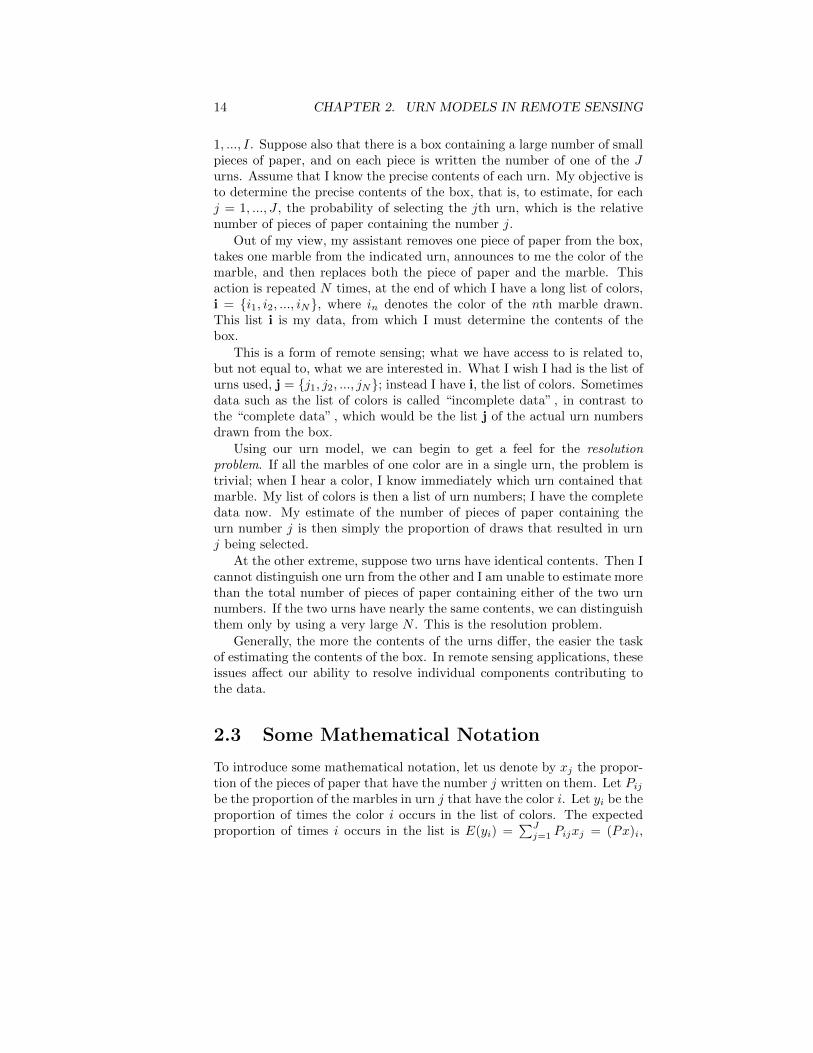


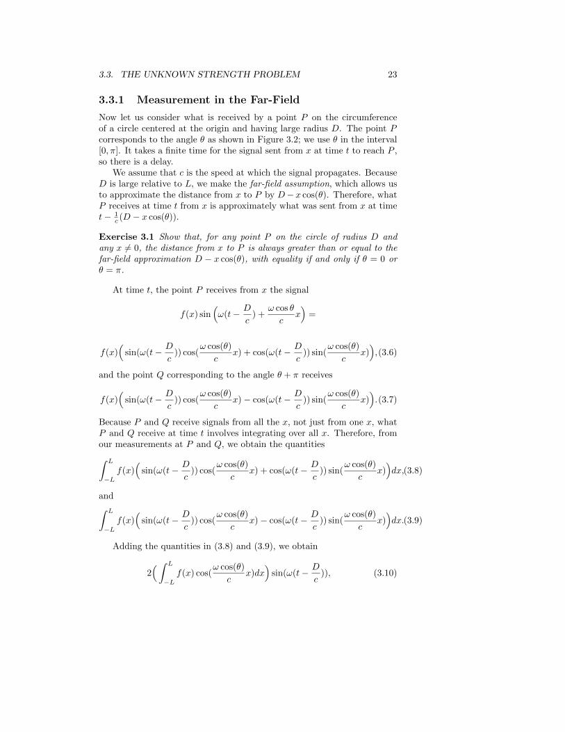


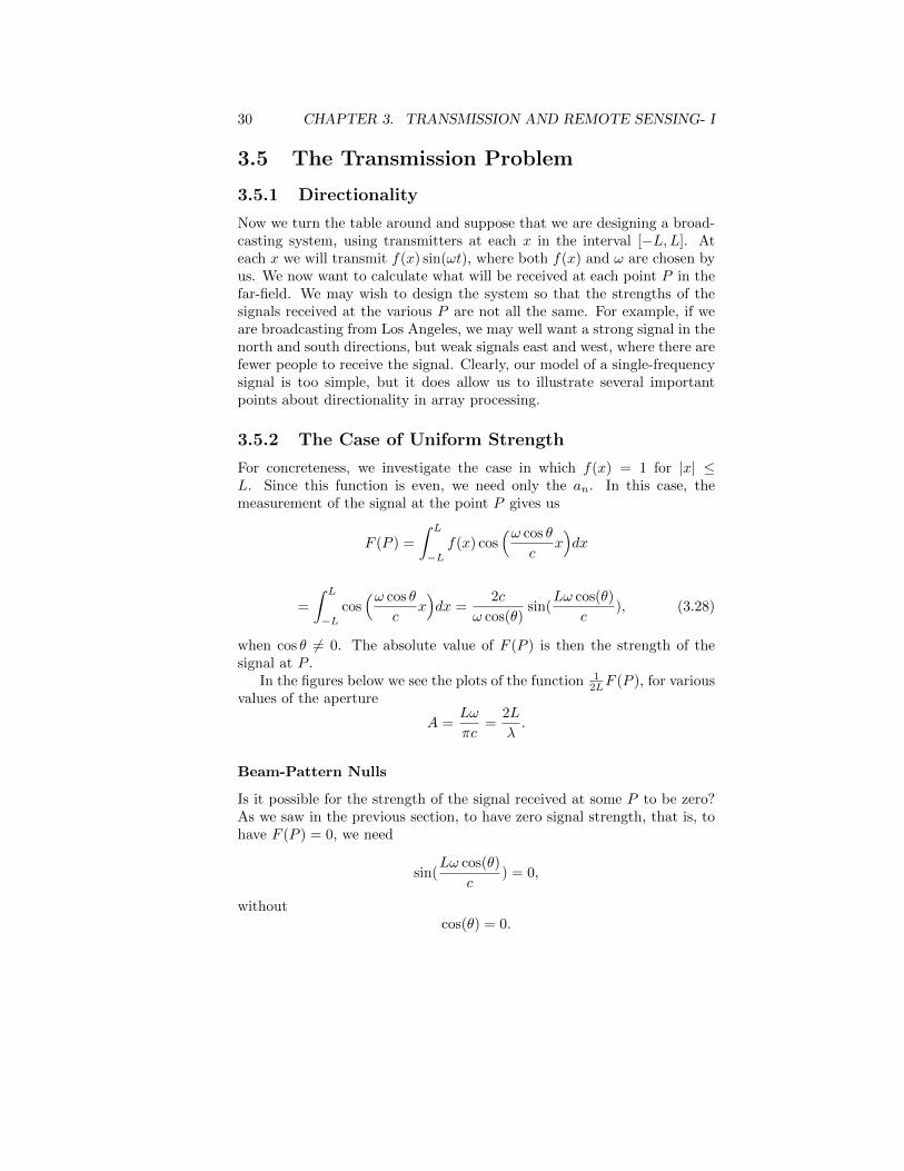


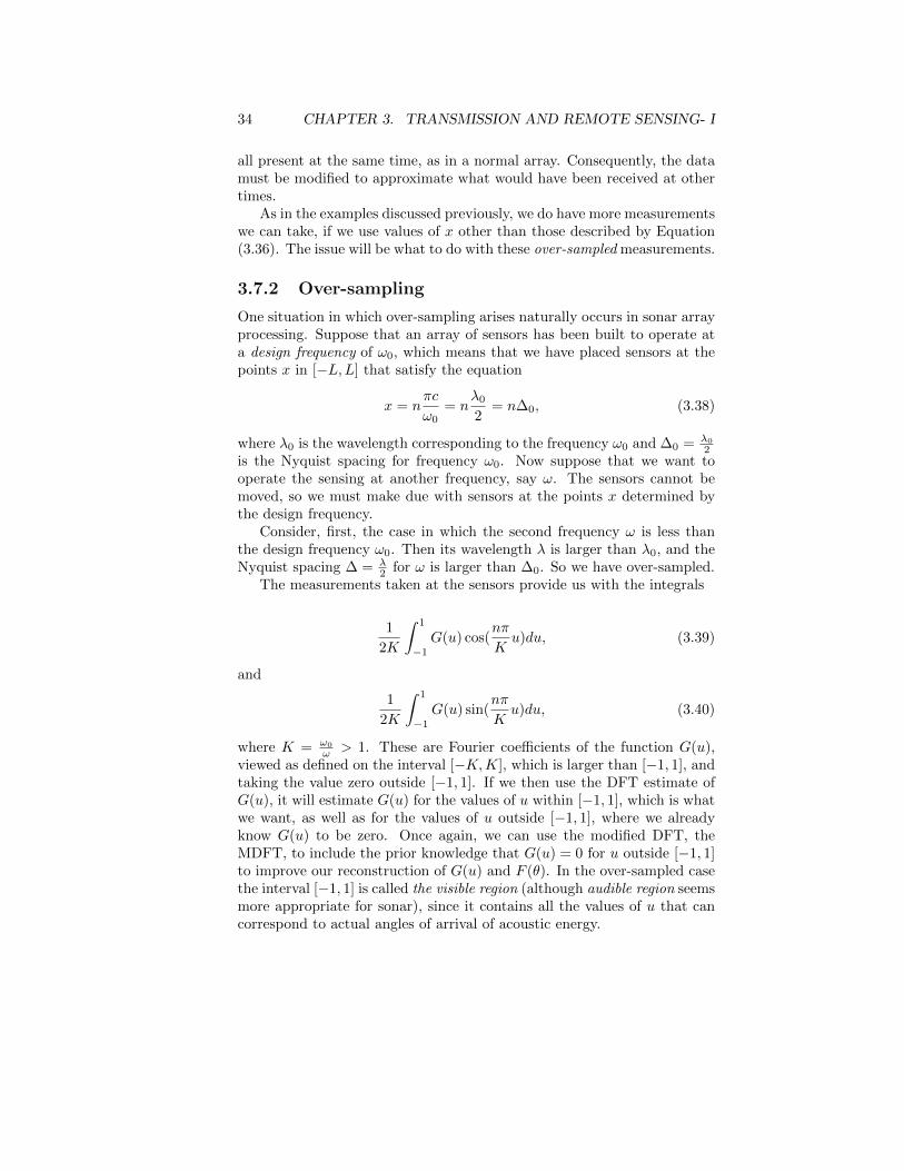
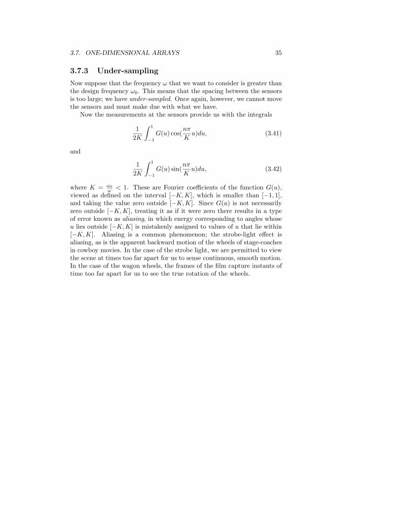


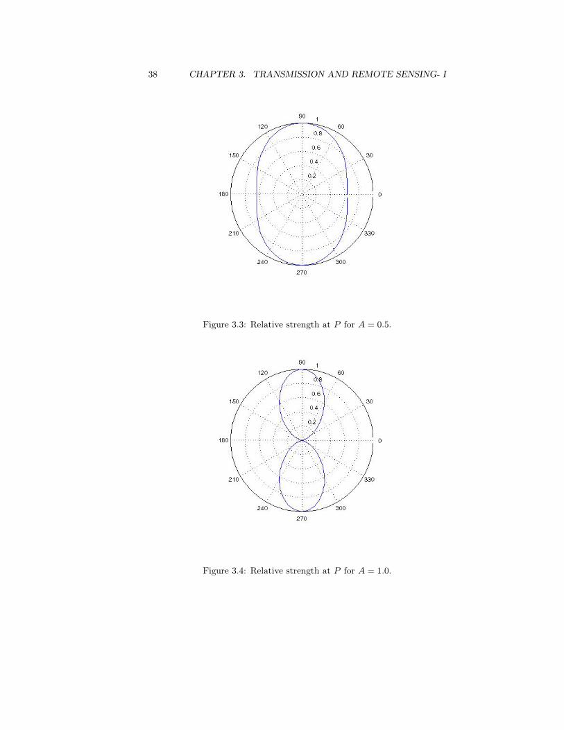
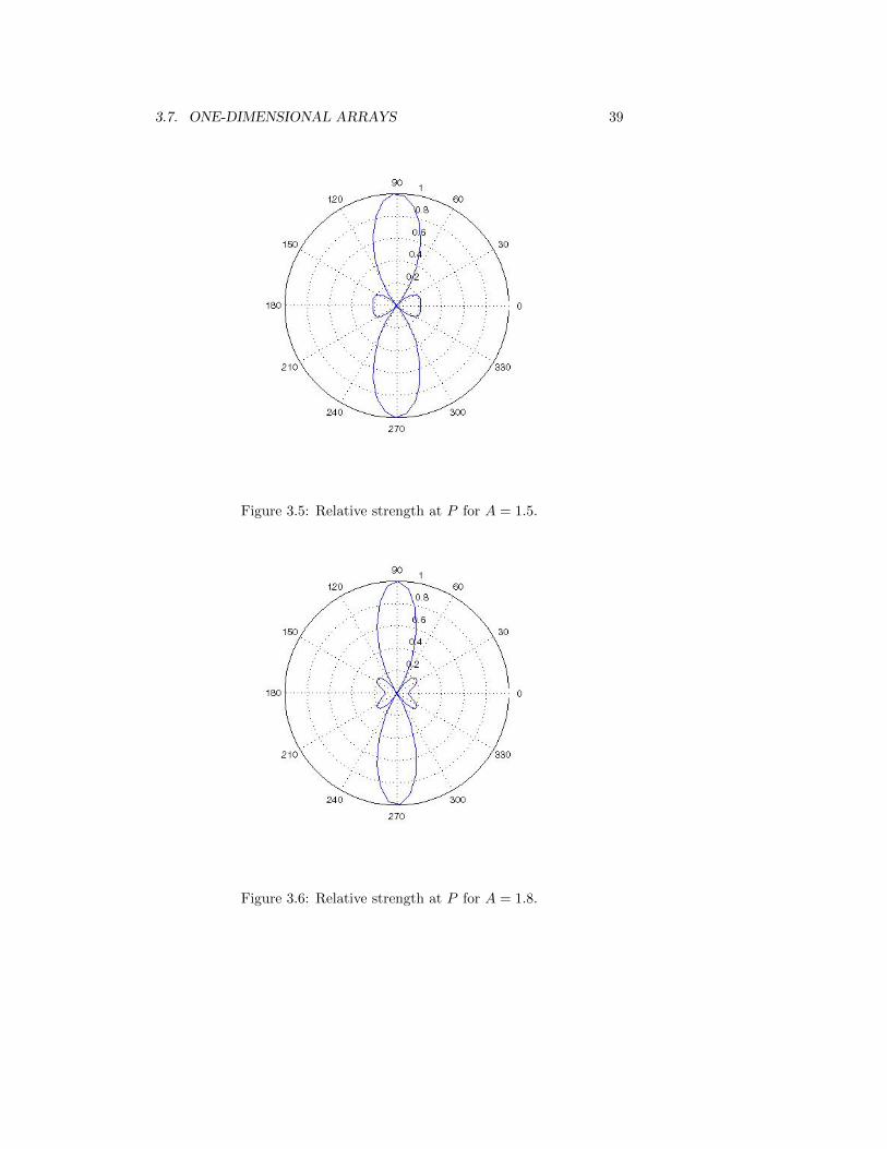


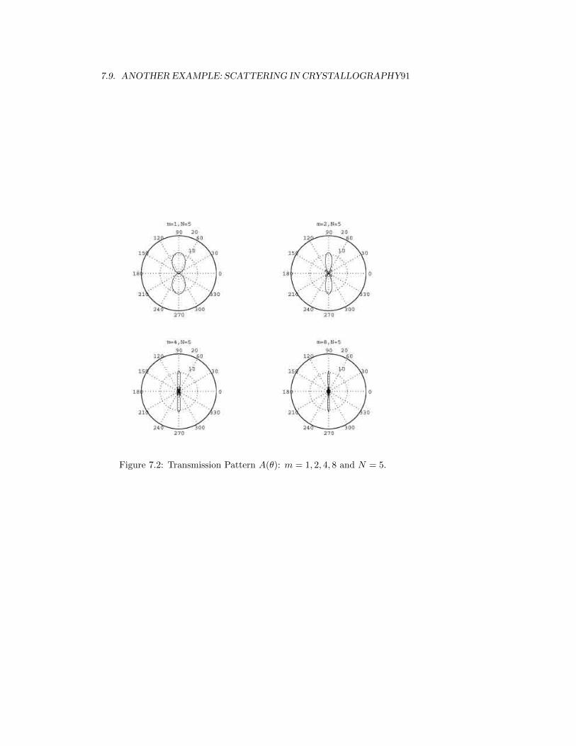
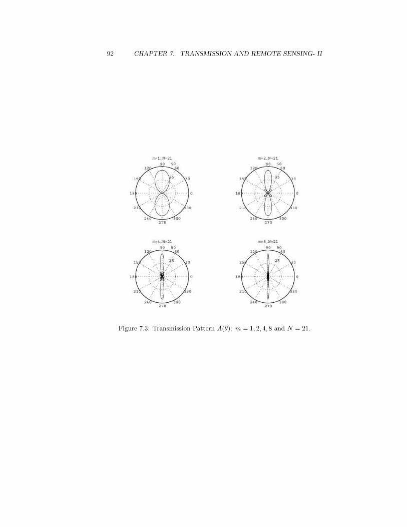


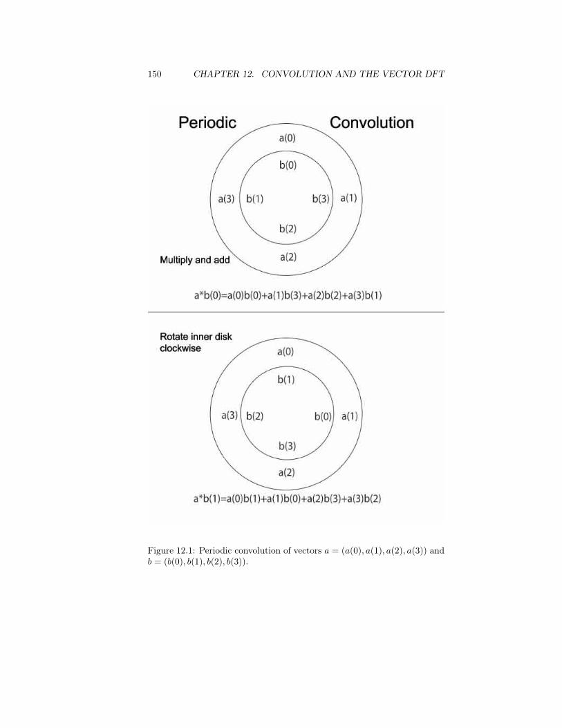


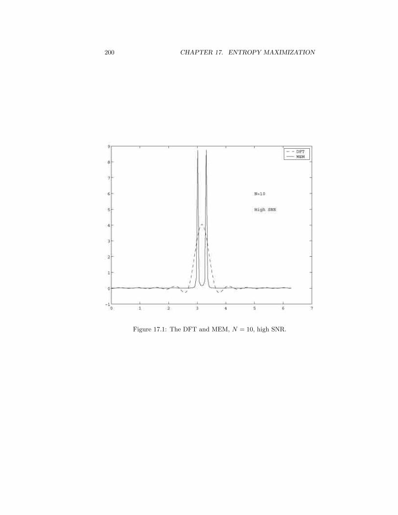


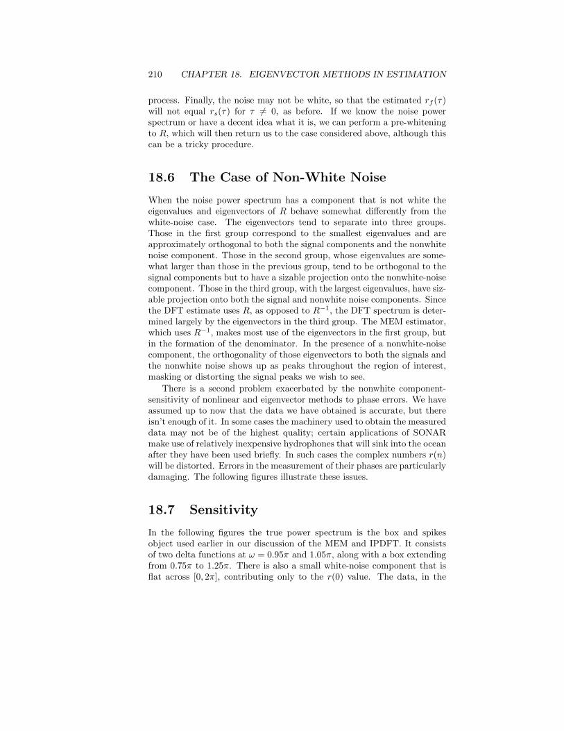


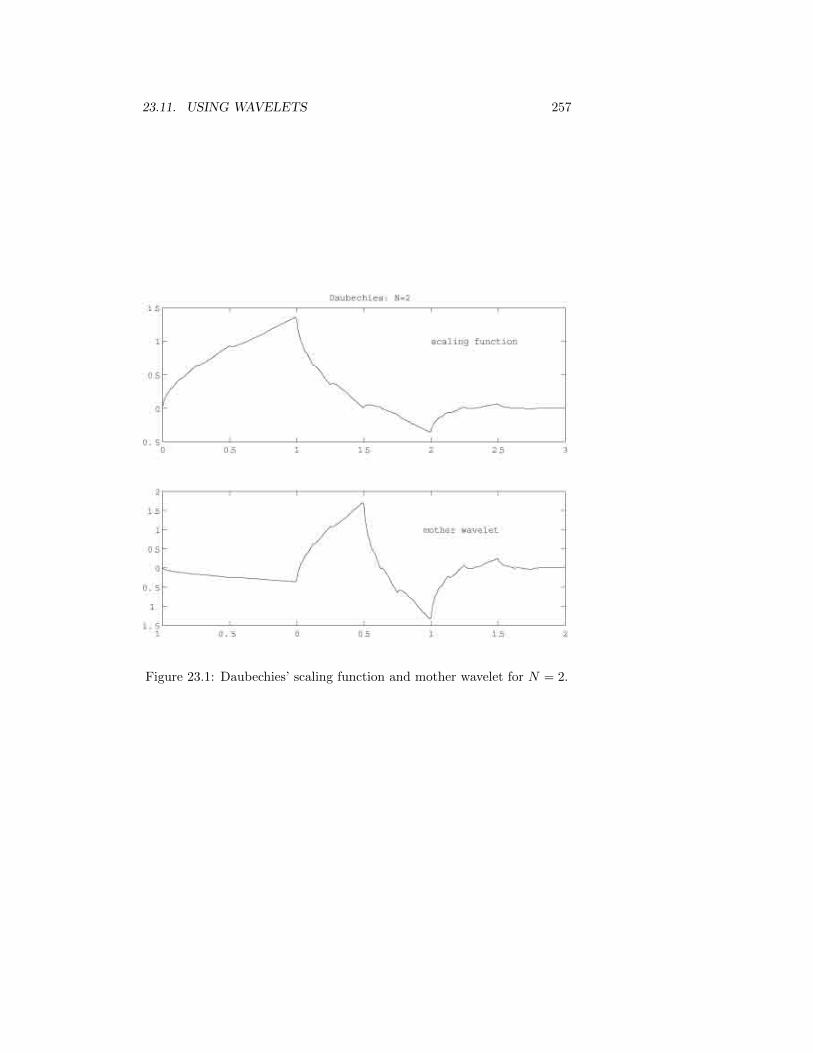


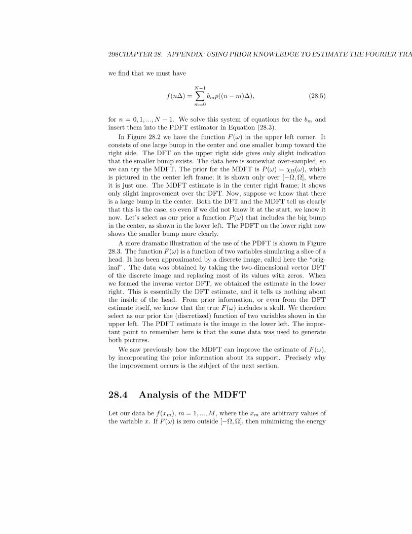


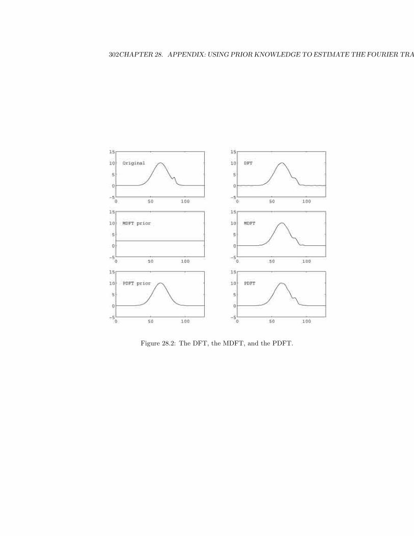


![ECE-V-DIGITAL SIGNAL PROCESSING [10EC52] …vtusolution.in/.../digital-signal-processing-10ec52.pdfDigital vtusolution.in Signal Processing 10EC52 TEXT BOOK: 1. DIGITAL SIGNAL PROCESSING](https://static.documents.pub/doc/80x56/5afe42bb7f8b9a256b8ccd2e/ece-v-digital-signal-processing-10ec52-signal-processing-10ec52-text-book.jpg)


