Matlab Tool in NM Image InTech Maria Lyra 2011

23

MATLAB as a Tool in Nuclear Medicine Image Processing

Maria Lyra, Agapi Ploussi and Antonios Georgantzoglou

Radiation Physics Unit, A’ Radiology Department, University of Athens Greece

1. Introduction Advanced techniques of image processing and analysis find widespread use in medicine. In medical applications, image data are used to gather details regarding the process of patient imaging whether it is a disease process or a physiological process. Information provided by medical images has become a vital part of today’s patient care. The images generated in medical applications are complex and vary notably from application to application. Nuclear medicine images show characteristic information about the physiological properties of the structures-organs. In order to have high quality medical images for reliable diagnosis, the processing of image is necessary. The scope of image processing and analysis applied to medical applications is to improve the quality of the acquired image and extract quantitative information from medical image data in an efficient and accurate way. MatLab (Matrix Laboratory) is a high performance interactive software package for scientific and engineering computation developed by MathWorks (Mathworks Inc., 2009). MatLab allows matrix computation, implementation of algorithms, simulation, plotting of functions and data, signal and image processing by the Image Processing Toolbox. It enables quantitative analysis and visualisation of nuclear medical images of several modalities, such as Single Photon Emission Computed Tomography (SPECT), Positron Emission Tomography (PET) or a hybrid system (SPECT/CT) where a Computed Tomography system (CT) is incorporated to the SPECT system. The Image Processing Toolbox (Mathworks Inc., 2009) is a comprehensive set of reference-standard algorithms and graphical tools for image processing, analysis, visualisation and algorithm development. It offers the possibility to restore noisy or degraded images, enhance images for improved intelligibility, extract features, analyse shapes and textures, and register two images. Thus, it includes all the functions that MatLab utilises in order to perform any sophisticated analysis needed after the acquisition of an image. Most toolbox functions are written in open MatLab language offering the opportunity to the user to inspect the algorithms, to modify the source code and create custom functions (Wilson et al., 2003, Perutka, 2010). This chapter emphasises on the utility of MatLab in nuclear medicine images’ processing. It includes theoretical background as well as examples. After an introduction to the imaging techniques in nuclear medicine and the quality of nuclear medicine images, this chapter proceeds to a study about image processing in nuclear medicine through MatLab. Image processing techniques presented in this chapter include organ contouring, interpolation,

MATLAB – A Ubiquitous Tool for the Practical Engineer

478

filtering, segmentation, background activity removal, registration and volume quantification. A section about DICOM image data processing using MatLab is also presented as this type of image is widely used in nuclear medicine.

2. Nuclear medicine imaging Nuclear Medicine is the section of science that utilises the properties of radiopharmaceuticals in order to derive clinical information of the human physiology and biochemistry. According to the examination needed for each patient, a radionuclide is attached to a pharmaceutical (tracer) and the whole complex is then delivered to the patient intravenously or by swallowing or even by inhalation. The radiopharmaceutical follows its physiological pathway and it is concentrated on specific organs and tissues for short periods of time. Then, the patient is positioned under a nuclear medicine equipment which can detect the radiation emitted by the human body resulting in images of the biodistribution of the radiopharmaceutical. In Nuclear Medicine, there are two main methods of patient imaging, the imaging with Planar Imaging, Dynamic Imaging or SPECT and the PET. During the last decade, hybrid systems have been developed integrating the CT technique with either SPECT or PET resulting in SPECT/CT and PET/CT respectively. This chapter will concentrate on the implementation of MatLab code in gamma camera planar imaging, SPECT and SPECT/CT methods. The gamma camera is composed of a collimator, a scintillator crystal usually made of NaI (or CsI), the photomultiplier tubes, the electronic circuits and a computer equipped with the suitable software to depict the nuclear medicine examinations. In planar imaging, the patient, having being delivered with the suitable radiopharmaceutical, is sited under the gamma camera head. The gamma camera head remains stable at a fixed position over the patient for a certain period of time, acquiring counts (disintegrations). These will constitute the radiopharmaceutical distribution image. The counts measured in a specific planar projection originate from the whole thickness of patient (Wernick & Aarsvold, 2004). In SPECT, the gamma camera head rotates around the patient remaining at well defined angles and acquiring counts for specific periods of time per angle. What makes SPECT a valuable tool in nuclear medicine is the fact that information in the three dimensions of the patient can be collected in a number of slices with a finite known volume (in voxels). Thus, SPECT technique is used to display the radiopharmaceutical distribution in a single slice removing the contribution from the overlying and underlying tissues. In order to obtain the most accurate quantitative data from SPECT images, two issues that have to be resolved are the attenuation correction and the Compton scattering that the photons are undergone until reach and interact with the slice of interest tissues. As an examining organ has certain dimensions, each slice along the axis of the gamma camera has different distance from the detector. Thus, each photon experiences different attenuation. These two phenomena usually lead to distortion of the measured activity concentration (Wernick & Aarsvold, 2004). The acquired data are processed in order to correct and compensate the undesired effect of these physical phenomena. The projection data of each slice constitute the sinogram. As a result, a series of sinograms is the files acquired. However, this kind of files needs reconstruction in order to get an image with diagnostic value. The most known reconstruction methods are the Filtered Back-Projection (FBP) and the Iterative methods.


479

Attenuation correction is resolved by using the constant linear attenuation coefficient (μ) method or using the transmission source method. In the first one, the distance that each photon has travelled is calculated based on the patient geometry and the exponential reduction of their intensity. Then, considering the human body as a uniform object, an attenuation map is implemented in the reconstructed image. The latter method utilises a transmission source which scans the patient. This depicts each pixel or voxel of the patient with a specific μ producing an attenuation coefficient map. Finally, the attenuation map is implemented on the image resulting in a more accurate diagnosis. The second issue of scatter correction can be resolved by the electronics of the gamma camera and the filtering process during reconstruction. When a photon undergoes scattering, its energy reduces. So, a well defined function can accept for imaging photons with energy at a certain narrow energy window around the central photopeak of the γ-emission. A hybrid SPECT/CT scanner is capable of implementing both a CT scan and a SPECT scan or it can be used for each of these scans separately. Using the CT scan, the anatomy of a specific patient area can be imaged while the SPECT scan can depict the physiology of this area. Then, the registration of the two images drives at an image of advanced diagnostic value. Moreover, the CT data is used for the implementation of attenuation correction. (Delbeke et al., 2006) The range of nuclear medicine examinations is fairly wide. It includes, among others, patients’ studies, as myocardium perfusion by 99mTc-Tetrofosmin or 99mTc-Sestamibi, striatum imaging in brain by 123I-Ioflupane (DaTSCAN), renal parenchyma imaging by 99mTc-De-Methylo-Sulfo-Acid (DMSA) and 99mTc-Methylo-Di-Phosphonate (MDP) for bone scintigraphy. Fundamental image analysis methods of myocardium, brain, kidneys, thyroid, lungs and oncological (e.g. neuroblastoma) nuclear medicine studies include regions’ properties, boundary analysis, curvature analysis or line and circle detection. Image processing serves in reconstruction of images acquired using SPECT techniques, in improvement of the quality of images for viewing and in preparation of images for quantitative results. Data of the mentioned examinations are used in the following applications of MatLab algorithms to make the image processing and analysis in nuclear medicine clear and show the MatLab utility for these studies.

2.1 Image quality in nuclear medicine Image quality plays an important role in nuclear medicine imaging as the goal is a reliable image of the projected organ to be provided, for accurate diagnosis or therapy. The physical characteristics that are used to describe image quality are (1) contrast, (2) spatial resolution and (3) noise. Image contrast is the difference in intensity corresponding to different concentration of activity in the patient. For high diagnostic accuracy, nuclear medicine images must be of high contrast. The image contrast is principally affected by the radiopharmaceutical that is used for imaging and the scattered radiation. In general, it is desirable to use a radiopharmaceutical which has a high uptake within the target organ. Spatial resolution is defined as the ability of the imaging modality to reproduce the details of a nonuniform radioactive distribution. The spatial resolution is separated into intrinsic resolution (scintillator, photomultiplier tubes and electronic circuit) and system resolution


480

(collimator, scintillator, photomultiplier tubes and electronic circuit). The intrinsic resolution depends on the thickness of scintillation crystal while the system resolution depends mainly on the distance from the emitting source to collimator. The resolution of a gamma camera is limited by several factors. Some of these are the patient motion, the statistical fluctuation in the distribution of visible photons detected and the collimators geometry (Wernick & Aarsvold, 2004). Noise refers to any unwanted information that prevents the accurate imaging of an object. Noise is the major factor in the degradation of image quality. Image noise may be divided into random and structured noise. Random noise (also referred as statistical noise) is the result of statistical variations in the counts being detected. The image noise is proportional to N1/2 where N is the number of detected photons per pixel. Therefore, as the number of counts increases the noise level reduces. Image noise is usually analysed in terms of signal-to-noise-ratio (SNR). SNR is equal to N/ N1/2. If the SNR is high, the diagnostic information of an image is appreciated regardless of the noise level. Structured noise is derived from non-uniformities in the scintillation camera and overlying structures in patient body.

2.2 Complex topics In the previous section, several issues arising from the need of achieving the best image quality have to be resolved. Sometimes, the whole procedure becomes really hard to be completed. Some concepts in image processing and analysis are theory-intensive and may be difficult for medical professionals to comprehend. Apart from that, each manufacturer uses different software environment for the application of reconstruction and presentation of the images. This drives at a lack of a standard pattern based on which a physician can compare or parallel two images acquired and reconstructed by nuclear imaging systems of different vendors. This is a node on which MatLab can meet a wide acceptance and utilisation. These complex topics can be analysed and resolved using MatLab algorithms to turn up the most effective techniques to emerge information through medical imaging.

3. Image analysis and processing in nuclear medicine In the last several decades, medical imaging systems have advanced in a dynamic progress. There have been substantial improvements in characteristics such as sensitivity, resolution, and acquisition speed. New techniques have been introduced and, more specifically, analogue images have been substituted by digital ones. As a result, issues related to the digital images’ quality have emerged. The quality of acquired images is degraded by both physical factors, such as Compton scattering and photon attenuation, and system parameters, such as intrinsic and extrinsic spatial resolution of the gamma camera system. These factors result in blurred and noisy images. Most times, the blurred images present artefacts that may lead to a fault diagnosis. In order the images to gain a diagnostic value for the physician, it is compulsory to follow a specific series of processing. Image processing is a set of techniques in which the data from an image are analysed and processed using algorithms and tools to enhance certain image information that is more useful to human interpretation (Nailon, 2010). The processing of an image permits the


481

extraction of useful parameters and increases the possibility of detection of small lesions more accurately. Image processing in nuclear medicine serves three major purposes: a) the reconstruction of the images acquired with tomographic (SPECT) techniques, b) the quality improvement of the image for viewing in terms of contrast, uniformity and spatial resolution and, c) the preparation of the image in order to extract useful diagnostic qualitative and quantitative information.

3.1 Digital images In all modern nuclear medicine imaging systems, the images are displayed as an array of discrete picture elements (pixels) in two dimensions (2D) and are referred as digital images. Each pixel in a digital image has an intensity value and a location address (Fig. 1). In a nuclear medicine image the pixel value shows the number of counts recorded in it. The benefit of a digital image compared to the analogue one is that data from a digital image are available for further computer processing.

Fig. 1. A digital image is a 2D array of pixels. Each pixel is characterised by its (x, y) coordinates and its value.

Digital images are characterised by matrix size, pixel depth and resolution. The matrix size is determined from the number of the columns (m) and the number of rows (n) of the image matrix (m×n). The size of a matrix is selected by the operator. Generally, as the matrix dimension increases the resolution is getting better (Gonzalez et al., 2009). Nuclear medicine images matrices are, nowadays, ranged from 64×64 to 1024×1024 pixels. Pixel or bit depth refers to the number of bits per pixel that represent the colour levels of each pixel in an image. Each pixel can take 2k different values, where k is the bit depth of the image. This means that for an 8-bit image, each pixel can have from 1 to 28 (=256) different colour levels (grey-scale levels). Nuclear medicine images are frequently represented as 8- or 16- bit images. The term resolution of the image refers to the number of pixels per unit length of the image. In digital images the spatial resolution depends on pixel size. The pixel size is calculated by the Field of View (FoV) divided by the number of pixels across the matrix. For a standard FoV, an increase of the matrix size decreases the pixel size and the ability to see details is improved.


482

3.2 Types of digital images – MatLab MatLab offers simple functions that can read images of many file formats and supports a number of colour maps. Depending on file type and colour space, the returned matrix is either a 2D matrix of intensity values (greyscale images) or a 3D matrix of RGB values. Nuclear medicine images are grey scale or true colour images (RGB that is Red, Green and Blue). The image types supported from the Image Processing Toolbox are listed below: • Binary Images. In these, pixels can only take 0 or 1 value, black or white. • Greyscale or intensity images. The image data in a greyscale image represent intensity

or brightness. The integers’ value is within the range of [0… 2k-1], where k is the bit depth of the image. For a typical greyscale image each pixel can represented by 8 bits and intensity values are in the range of [0…255], where 0 corresponds to black and 255 to white.

• True color or RGB. In these, an image can be displayed using three matrices, each one corresponding to each of red-green-blue colour. If in an RGB image each component uses 8 bits, then the total number of bits required for each pixel is 3×8=24 and the range of each individual colour component is [0…255].

• Indexed images. Indexed images consist of a 2D matrix together with an m×3 colour map (m= the number of the columns in image matrix). Each row of map specifies the red, green, and blue components of a single colour. An indexed image uses direct mapping of pixel values to colour map values. The colour of each image pixel is determined by using the corresponding value of matrix as an index into map.

The greyscale image is the most convenient and preferable type utilised in nuclear medicine image processing. When colouring depiction is needed, the RGB one should be used and processed. The indexed type images should be converted to any of the two other types in order to be processed. The functions used for image type conversion are: rgb2gray, ind2rgb, ind2gray and reversely. Any image can be also transformed to binary one using the command: im2bw. Moreover, in any image, the function impixelinfo can be used in order to detect any pixel value. The user can move the mouse cursor inside the image and the down left corner appears the pixel identity (x, y) as well as the (RGB) values. The pixel range of the image can be displayed by the command imdisplayrange.

3.3 MatLab image tool The Image Tool is a simple and user-friendly toolkit which can contribute to a quick image processing and analysis without writing a code and use MatLab language. These properties makes it a very useful tool when deep analysis is not the ultimate goal but quick processing for better view is desirable. The Image Tool opens by simply writing the command imtool in the main function window. Then a new window opens and the next step is loading an image. In the menu, there are many functions already installed in order to use it as simple image processing software. The tools include image information appearance, image zooming in and out, panning, adjustment of the window level and width, adjustment of contrast, cropping, distance measurement, conversion of the image to a pixel matrix and colour map choices (grey scale, bone colour, hot regions among others). These are the most common functions likely to be performed in the initial processing approach. Moreover, the user can make some further manipulations such as 3D rotation to respective 3D images and plotting of pixel data.


483

3.4 Image processing techniques - MatLab Image processing techniques include all the possible tools used to change or analyse an image according to individuals’ needs. This subchapter presents the most widely performed image processing techniques that are applicable to nuclear medicine images. The examples used are mostly come from nuclear medicine renal studies, as kidneys’ planar images and SPECT slices are simple objects to show the application of image processing MatLab tools.

3.4.1 Contrast enhancement One of the very first image processing issues is the contrast enhancement. The acquired image does not usually present the desired object contrast. The improvement of contrast is absolutely needed as the organ shape, boundaries and internal functionality can be better depicted. In addition, organ delineation can be achieved in many cases without removing the background activity. The command that implements contrast processing is the imadjust. Using this, the contrast in an image can be enhanced or degraded if needed. Moreover, a very useful result can be the inversion of colours, especially in greyscale images, where an object of interest can be efficiently outlined. The general function that implements contrast enhancement is the following:

J = imadjust(I,[low_in high_in],[low_out high_out],gamma);

while the function for colour inversion is the following:

J = imadjust(I,[0 1],[1 0],gamma); or J = imcomplement(I);

suppose that J, is the new image, I, is the initial image and gamma factor depicts the shape of the curve that describes the relationship between the values of I and J. If the gamma factor is omitted, it is considered to be 1.

3.4.2 Organ contour In many nuclear medicine images, the organs’ boundaries are presented unclear due to low resolution or presence of high percentage of noise. In order to draw the contour of an organ in a nuclear medicine image, the command imcontour is used. In addition, a variable n defines the number of equally spaced contours required. This variable is strongly related with the intensity of counts. For higher n values, the lines are drawn with smaller spaces in between and depict different streaks of intensity. The type of line contouring can be specified as well. For example, when a contour of 5 level contours, drawn with solid line, is the desirable outcome, the whole function is:

Example 1I = imread(‘kindeys.jpg’); figure, imshow(I) J = imcontour(I,5,’-‘); Figure, imshow(J) where J and I stands for the final and the initial image respectively and the symbol (’-‘) stands for the solid line drawing. An example of the initial image, the contour with n=15 and n=5 respectively, follows.


484

Fig. 2. (a) Original image depicting kidneys, (b) organs contoured with n = 15, (c) organs contoured with n = 5.

3.4.3 Image interpolation Interpolation is a topic that has been widely used in image processing. It constitutes of the most common procedure in order to resample an image, to generate a new image based on the pattern of an existing one. Moreover, re-sampling is usually required in medical image processing in order to enhance the image quality or to retrieve lost information after compression of an image (Lehmann et al., 1999). Interpreting the interpolation process, the user is provided with several options. These options include the resizing of an image according to a defined scaling factor, the choice of the interpolation type and the choice of low-pass filter. The general command that performs image resizing is imresize. However, the way that the whole function has to be written depends heavily on the characteristics of the new image. The size of the image can be defined as a scaling factor of the existing image or by exact number of pixels in rows and columns. Concerning the interpolation types usually used in nuclear medicine, these are the following: a) nearest-neighbour interpolation (‘nearest’), where the output pixel obtains the value of the pixel that the point falls within, without considering other pixels, b) bilinear interpolation (‘bilinear’), where the output pixel obtains a weighted average value of the nearest 2x2 pixels, c) cubic interpolation (‘bicubic’), where the output pixel obtains a weighted average value of the nearest 4x4 pixels (Lehmann et al., 1999). When an image has to resize in a new one, with specified scaling factor and method, then the function Implementing that, is the following:

NewImage = imresize(Image, scale, method);

For example, for a given image I, the new image J shrunk twice of the initial one, using the bilinear interpolation method, the function will be:

J = imresize(I, 0.5, ‘bilinear’);

This way of image resizing contributes to the conversion of image information during any such process, a fact that is valuable in the precision of a measurement. Bilinear interpolation is often used to zoom into a 2D image or for rendering, for display purposes. Apart from the previous methods, the cubic convolution method can be applied to 3D images.

3.4.4 Image filtering The factors that degrade the quality of nuclear medicine images result in blurred and noisy images with poor resolution. One of the most important factors that greatly affect the


485

quality of clinical nuclear medicine images is image filtering. Image filtering is a mathematical processing for noise removal and resolution recovery. The goal of the filtering is to compensate for loss of detail in an image while reducing noise. Filters suppressed noise as well as deblurred and sharpened the image. In this way, filters can greatly improve the image resolution and limit the degradation of the image. An image can be filtered either in the frequency or in the spatial domain. In the first case the initial data is Fourier transformed, multiplied with the appropriate filter and then taking the inverse Fourier transform, re-transformed into the spatial domain. The basics steps of filtering in the frequency domain are illustrated in Fig. 3.

Fig. 3. Basics steps of frequency domain filtering.

The filtering in the spatial domain demands a filter mask (it is also referred as kernel or convolution filter). The filter mask is a matrix of odd usually size which is applied directly on the original data of the image. The mask is centred on each pixel of the initial image. For each position of the mask the pixel values of the image is multiplied by the corresponding values of the mask. The products of these multiplications are then added and the value of the central pixel of the original image is replaced by the sum. This must be repeated for every pixel in the image. The procedure is described schematically in Fig. 4. If the filter, by which the new pixel value was calculated, is a linear function of the entire pixel values in the filter mask (e.g. the sum of products), then the filter is called linear. If the output pixel is not a linear weighted combination of the input pixel of the image then the filtered is called non-linear. According to the range of frequencies they allow to pass through filters can be classified as low pass or high pass. Low pass filters allow the low frequencies to be retained unaltered and block the high frequencies. Low pass filtering removes noise and smooth the image but at the same time blur the image as it does not preserve the edges. High pass filters sharpness the edges of the image (areas in an image where the signal changes rapidly) and enhance object edge information. A severe disadvantage of high pass filtering is the amplification of statistical noise present in the measured counts. The next section is referred to three of the most common filters used by MatLab: the mean, median and Gaussian filter.


486

Fig. 4. Illustration of filtering process in spatial domain.

3.4.4.1 Mean filter Mean filter is the simplest low pass linear filter. It is implemented by replacing each pixel value with the average value of its neighbourhood. Mean filter can be considered as a convolution filter. The smoothing effect depends on the kernel size. As the kernel size increases, the smoothing effect increases too. Usually a 3×3 (or larger) kernel filter is used. An example of a single 3×3 kernel is shown in the Fig. 5.

Fig. 5. Filtering approach of mean filter.

The Fig.5 depicts that by using the mean filter, the central pixel value would be changed from “e” to ‘’ (a+b+c+d+e+f+g+h+i) 1/9’’. 3.4.4.2 Median filter Median filter is a non linear filter. Median filtering is done by replacing the central pixel with the median of all the pixels value in the current neighbourhood. A median filter is a useful tool for impulse noise reduction (Toprak & Göller, 2006). The impulse noise (it is also known as salt and paper noise) appears as black or (/and) white


487

pixels randomly distributed all over the image. In other words, impulse noise corresponds to pixels with extremely high or low values. Median filters have the advantage to preserve edges without blurring the image in contrast to smoothing filters.

Fig. 6. Filtering approach of Median Filter.

3.4.4.3 Gaussian filter Gaussian filter is a linear low pass filter. A Gaussian filter mask has the form of a bell-shaped curve with a high point in the centre and symmetrically tapering sections to either side (Fig.7). Application of the Gaussian filter produces, for each pixel in the image, a weighted average such that central pixel contributes more significantly to the result than pixels at the mask edges (O’Gorman et al., 2008). The weights are computed according to the Gaussian function (Eq.1):

2 21 ( ) /(2 )( )

2xf x e μ σ

σ π− −= (1)

where μ, is the mean and σ, the standard deviation.

Fig. 7. A 2D Gaussian function.

The degree of smoothing depends on the standard deviation. The larger the standard deviation, the smoother the image is depicted. The Gaussian filter is very effective in the reduction of impulse and Gaussian noise. Gaussian noise is caused by random variations in the intensity and has a distribution that follows the Gaussian curve.


488

3.5 Filtering in MatLab In MatLab, using Image Processing Toolbox we can design and implemented filters for image data. For linear filtering, MatLab provides the fspecial command to generate some predefined common 2D filters.

h=fspecial(filtername, parameters)

The filtername is one of the average, disk, gaussian, laplacian, log, motion, prewitt, sobel and unsharp filters; that is the parameters related to the specific filters that are used each time. Filters are applied to 2D images using the function filter2 with the syntax:

Y = filter2(h,X)

The function filter2 filters the data in matrix X with the filter h. For multidimensional images the function imfilter is used.

B = imfilter(A,h)

This function filters the multidimensional array A with the multidimensional filter h. imfilter function is more general than filter2 function. For nonlinear filtering in MatLab the function nlfilter is applied, requiring three arguments: the input image, the size of the filter and the function to be used.

B = nlfilter(A, [m n], fun)

Example 2 The following example describes the commands’ package that can be used for the application of the mean (average) filter in a SPECT slice for different convolution kernel sizes (for 3×3, 9×9, 25×25 average filter).

h=fspecial('average', [3 3]); b=imfilter(a,h); figure, imshow(b); i=fspecial('average', [9 9]); c=imfilter(b,h); figure, imshow(c); j=fspecial('average', [25 25]); d=imfilter(c,h); figure, imshow(d);

Figure 8 presents different implementations of the mean filter on a kidneys image with filters 3x3, 9x9, 15x15, 20x20 and 25x25. As it can be easily noticed, the mean filter balances and smoothes the image, flattening the differences. The filtered images do not present edges at the same extent as in the original one. For larger kernel size, the blurring of the image is more intense. Image smoothening can be used in several areas of nuclear medicine and can serve in different points of view of the examined organ.

Example 3

In this example we will try to remove impulse noise from a SPECT slice, for example in a renal study. For this reason we mix the image with impulse noise (salt and pepper). The image has a 512×512 matrix size and grey levels between 0 and 255. The most suitable filter


489

for removing impulse noise is the median filter. Because it is a nonlinear filter, the command nlfilter is now used.

Fig. 8. Mean filter applied on kidneys image (a) Original image, (b) average filter 3x3, (c) average filter 9x9, (d) average filter 15x15, (e) average filter 20x20 and, (f) average filter 25x25 [(a) to (f) from left to right].

I = imread('kidneys.tif'); figure, imshow(I); J = imnoise(I,'salt & pepper',0.05); figure, imshow(J); fun = @(x) median(x(:)); K = nlfilter(J,[3 3],fun); figure, imshow(K);

Fig. 9. Impulse noise elimination by median filter. (a) Original image (b) the image with impulse noise (c) the image on which the noise is suppressed with the median filter. [(a) to (c) from left to right]


490

Example 3 can be very useful in the nuclear medicine examinations of parenchymatous organs (liver, lungs, thyroid or kidneys) as it consists of a simple enough method for the reduction of noise which interferes in the image due to the construction of electronic circuits.

3.6 Image segmentation The image segmentation describes the process through which an image is divided into constituent parts, regions or objects in order to isolate and study separately areas of special interest. This process assists in detecting critical parts of a nuclear medicine image that are not easily displayed in the original image. The process of segmentation has been developed based on lots of intentions such as delineating an object in a gradient image, defining the region of interest or separating convex components in distance-transformed images. Attention should be spent in order to avoid ‘over-segmentation’ or ‘under-segmentation’. In nuclear medicine, segmentation techniques are used to detect the extent of a tissue, an organ, a tumour inside an image, the boundaries of structures in cases that these are ambiguous and the areas that radiopharmaceutical concentrate in a greater extent. Thus, the segmentation process serves in assisting the implementation of other procedures; in other words, it constitutes the fundamental step of some basic medical image processing (Behnaz et al., 2010). There are two ways of image segmentation: a) based on the discontinuities and, b) based on the similarities of structures inside an image. In nuclear medicine images, the discontinuity segmentation type finds more applications. This type depends on the detection of discontinuities or else, edges, inside the image using a threshold. The implementation of threshold helps in two main issues: i) the removal of unnecessary information from the image (background activity) and, ii) the appearance of details not easily detected. The edge detection uses the command edge. In addition, a threshold is applied in order to detect edges above defined grey-scale intensity. Also, different methods of edge detection can be applied according to the filter each of them utilises. The most useful methods in nuclear medicine are the ‘Sobel’, ‘Prewitt’, ‘Roberts’, ‘Canny’ as well as ‘Laplacian of Gaussian'. It is noted that the image is immediately transformed into a binary image and edges are detected. The general function used for the edge detection is the following:

[BW] = edge (image, ‘method’, threshold)

Where [BW] is the new binary image produced, image is the initial one; ‘method’ refers to the method of edge detection and ‘threshold’ to the threshold applied. In nuclear medicine, the methods that find wide application are the sorbel, prewitt and canny. In the following example, the canny method is applied in order to detect edges in an image.

Example 4

I = imread(‘kidneys.jpg’); figure, imshow(I) J = edge(I,'canny', 0.048); figure, imshow(J)

Another application of segmentation in nuclear medicine is the use of gradient magnitude. The original image is loaded. Then, the edge detection method of sobel is applied in accordance with a gradient magnitude which gives higher regions with higher grey-scale intensity. Finally, the foreground details are highlighted and segmented image of the kidneys is produced. The whole code for that procedure is described below.


491

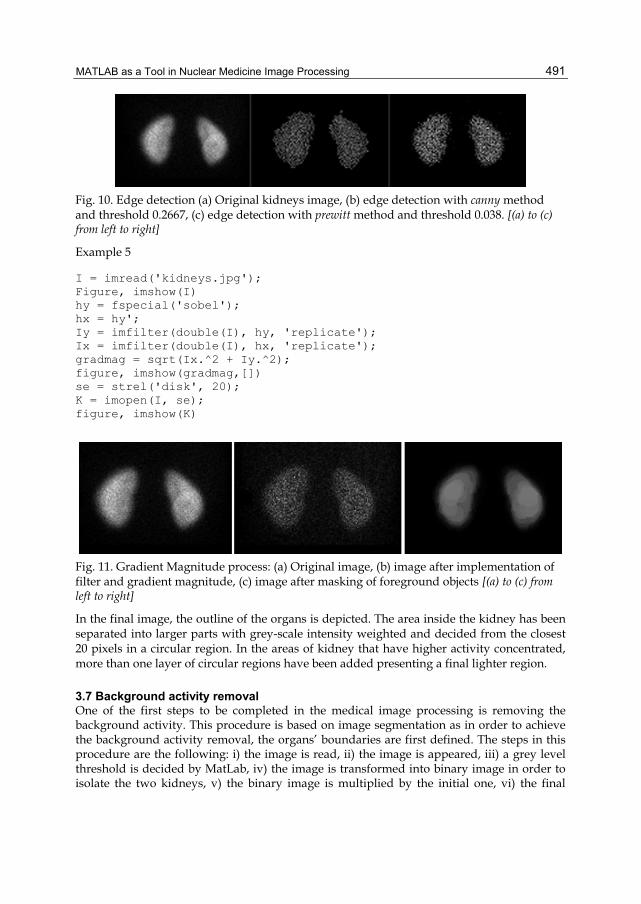
Fig. 10. Edge detection (a) Original kidneys image, (b) edge detection with canny method and threshold 0.2667, (c) edge detection with prewitt method and threshold 0.038. [(a) to (c) from left to right]

Example 5

I = imread('kidneys.jpg'); Figure, imshow(I) hy = fspecial('sobel'); hx = hy'; Iy = imfilter(double(I), hy, 'replicate'); Ix = imfilter(double(I), hx, 'replicate'); gradmag = sqrt(Ix.^2 + Iy.^2); figure, imshow(gradmag,[]) se = strel('disk', 20); K = imopen(I, se); figure, imshow(K)

Fig. 11. Gradient Magnitude process: (a) Original image, (b) image after implementation of filter and gradient magnitude, (c) image after masking of foreground objects [(a) to (c) from left to right]

In the final image, the outline of the organs is depicted. The area inside the kidney has been separated into larger parts with grey-scale intensity weighted and decided from the closest 20 pixels in a circular region. In the areas of kidney that have higher activity concentrated, more than one layer of circular regions have been added presenting a final lighter region.

3.7 Background activity removal One of the first steps to be completed in the medical image processing is removing the background activity. This procedure is based on image segmentation as in order to achieve the background activity removal, the organs’ boundaries are first defined. The steps in this procedure are the following: i) the image is read, ii) the image is appeared, iii) a grey level threshold is decided by MatLab, iv) the image is transformed into binary image in order to isolate the two kidneys, v) the binary image is multiplied by the initial one, vi) the final


492

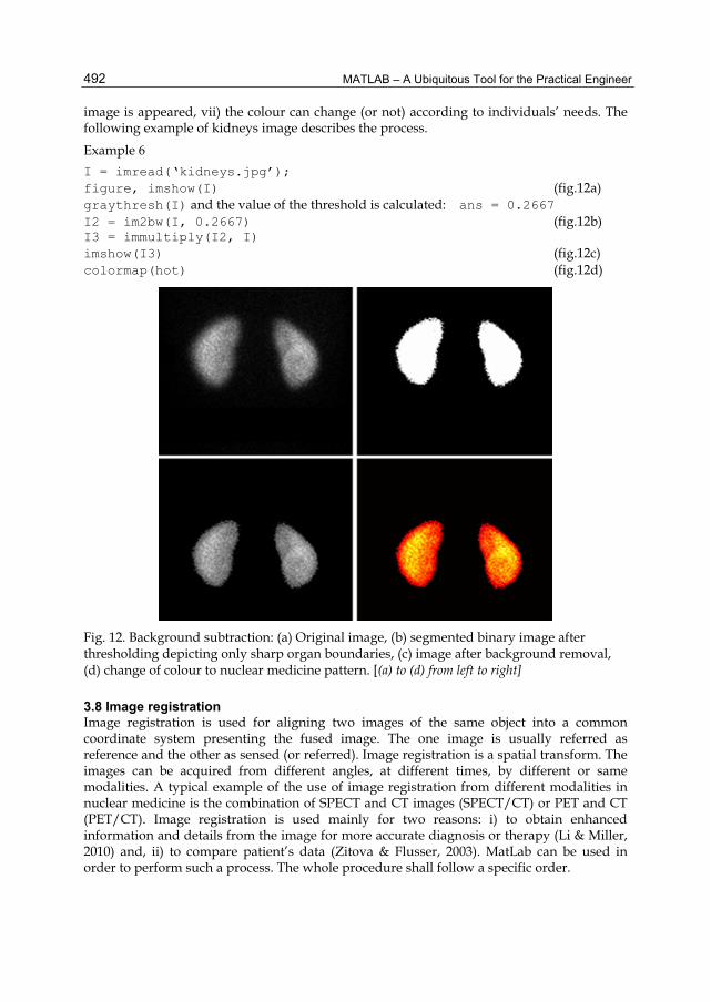
image is appeared, vii) the colour can change (or not) according to individuals’ needs. The following example of kidneys image describes the process. Example 6 I = imread(‘kidneys.jpg’); figure, imshow(I) (fig.12a) graythresh(I) and the value of the threshold is calculated: ans = 0.2667 I2 = im2bw(I, 0.2667) (fig.12b) I3 = immultiply(I2, I) imshow(I3) (fig.12c) colormap(hot) (fig.12d)

Fig. 12. Background subtraction: (a) Original image, (b) segmented binary image after thresholding depicting only sharp organ boundaries, (c) image after background removal, (d) change of colour to nuclear medicine pattern. [(a) to (d) from left to right]

3.8 Image registration Image registration is used for aligning two images of the same object into a common coordinate system presenting the fused image. The one image is usually referred as reference and the other as sensed (or referred). Image registration is a spatial transform. The images can be acquired from different angles, at different times, by different or same modalities. A typical example of the use of image registration from different modalities in nuclear medicine is the combination of SPECT and CT images (SPECT/CT) or PET and CT (PET/CT). Image registration is used mainly for two reasons: i) to obtain enhanced information and details from the image for more accurate diagnosis or therapy (Li & Miller, 2010) and, ii) to compare patient’s data (Zitova & Flusser, 2003). MatLab can be used in order to perform such a process. The whole procedure shall follow a specific order.


493

The first step of the procedure includes the image acquisition. After that, each image is reconstructed separately. Any filters needed are applied as well as enhancements in brightness and contrast. The process of filter application has been described in a previous section. The next step includes the foundation of a spatial transformation between the two images, the one of SPECT and the other of CT. The key figure in this step concerns about the alignment of the two images. A spatial transformation modifies the spatial relationship between the pixels of an image relocating them to new positions in a new image. There are several types of spatial transformation including the affine, the projective the box and the composite (Delbeke et al., 2006). The final step in image registration is the overlapping of the two images allowing a suitable level of transparency. A new image is created containing information from both pictures from which, the first has been produced. The whole procedure can be described with a set of commands which is user customised as different registration function packages can be constructed for different uses.

3.9 Intensity volume and 3-D visualisation Volume visualisation in nuclear medicine consists of a method for extracting information from volumetric data utilising and processing a nuclear medicine image (Lyra et al., 2010b). In MatLab, this can be achieved by constructing a 3D surface plot which uses the pixel identities for (x, y) axes and the pixel value is transformed into surface plot height and, consequently, colour. Apart from that, 3D voxel images can be constructed; SPECT projections are acquired, iso-contours are depicted on them including a number of voxels and, finally all of them can be added in order to create the desirable volume image. (Lyra et al., 2010a). Volume rendering - very often used in 3D SPECT images - is an example of efficient coding in MatLab. Inputs to the function are the original 3D array, the position angle, zoom or focus of the acquired projections. The volume rendering used in 3D myocardium, kidneys, thyroid, lungs and liver studies, took zoom and angles of 5.6 degrees, a focal length in pixels depending of the organs’ size. The size of the re-projection is the same as the main size of input image (e.g. 128x128 for the 128x128x256 input image). The volume rendering by MatLab is slow enough but similar to other codes’ volume rendering. An example image of myocardial 3-D voxel visualisation follows (Fig. 13):

Fig. 13. 3D myocardial voxel visualisation; the image does not depicts the real volume but the voxelised one (Lyra et al 2010a).


494

4. MatLab mesh plot MatLab is unique in data analysis in neurological imaging. We used MatLab and the functions of Image Processing Toolbox, to extract 3D basal ganglia activity measurements in dopamine transporters DaTSCAN scintigraphy. It can be easily run in an ordinary computer with Windows software, provides reproducible - user independent - results allowing better follow-up control comparing to the semi-quantitative evaluation of tracer uptake in basal ganglia. The surface plot or the mesh plot can be used in order to extract information about the consistency of an organ or the loss of functionality. In order to construct a surface plot from a striatum image, the series of images that include the highest level of information was selected (Lyra et al 2010b) (Fig. 14):

Fig. 14. A Series of central 123I-DaTSCAN SPECT imaging slices of I-123/Ioflupane; uptake is highest in middle 4 slices, and these were summarized for region of interest analysis (Lyra et al 2010b).

After the selection, ROI analysis was performed in order to concentrate on the area of interest which is the middle site of the image. The area of interest was selected and a package of functions was implemented. Example 7

I = imread(‘striatum.jpg’); figure, imshow(I) [x,y] = size(I); X = 1:x; Y = 1:y; [xx,yy] = meshgrid(Y,x); J = im2double(I); figure, surf(xx,yy,J); shading interp view(-40,60)

The whole procedure was, finally, resulted in the surface plot that is presented in the Fig. 15. A point of interest could be that although the images that were used to construct the surface plot were small and blurred, the final plot is clear and gives a lot of information regarding the activity concentration in these two lobes. The angle of view can


495

be defined by the user giving the opportunity to inspect the whole plot from any point of view.

Fig. 15. Surface Plot of pixel intensity; x and y axes represent the pixels identities while the z axis represents the pixel intensity.

5. DICOM image processing using MatLab The digital medical image processing started with the development of a standard for transferring digital images in order to enable users to retrieve images and related information from different modalities with a standardised way that is identical for all imaging modalities. In 1993, a new image format was established by National Electrical Manufacturers Association (NEMA). The Digital Imaging and Communication in Medicine (DICOM) standard allows the communication between equipment from different modalities and vendors facilitating the management of digital images. The DICOM standard defines a set of common rules for the exchange, storage and transmission of digital medical images with their accompanying information (Bidgood & Horii, 1992). A DICOM file consists of the data header (so called metadata) and the DICOM image data set. The header includes image related information such as image type, study, modality,


496

matrix dimensions, number of stored bits, patient’s name. The image data follow the header and contains 3D information of the geometry (Bankman, 2000). The DICOM files have a .dcm extension.

Fig. 16. Posterior image of kidneys in a DICOM format.

In nuclear medicine, the most common and supported format for storing 3D data using DICOM is to partition the volume (as myocardium or kidneys) into slices and to save each slice as a simple DICOM image. The slices can be distinguished either by a number coding in the file name or by specific DICOM tags. MatLab supports DICOM files and is a very useful tool in the processing of DICOM images. An example of reading and writing metadata and image data of a DICOM file using MatLab is given in the next section. Let us consider a planar projection from a kidneys scan study for a 10-month-old boy as the DICOM image (Fig. 16). The specific DICOM image is a greyscale image. Assuming “kidneys” is the name of the DICOM image we want to read, in order to read the image data from the DICOM file use the command dicomread in the following function.

I = dicomread('kidneys.dcm');

To read metadata from a DICOM file, use the dicominfo command. The latter returns the information in a MatLab structure where every field contains a specific piece of DICOM metadata. For the same DICOM image as previously,

info = dicominfo('kidneys.dcm')

A package of information appears in the command window including all the details that accompany a DICOM image. This is a great advantage of this image format in comparison to jpeg or tiff formats as the images retain all the information whereas the jpeg or tiff ones lose a great majority of it. For the specific image, the following information appears:

info = Filename: 'kidneys.dcm' FileModDate: '17-Feb-2011 14:04:18' FileSize: 128000 Format: 'DICOM' FormatVersion: 3 Width: 256 Height: 256 BitDepth: 16


497

ColorType: 'grayscale' FileMetaInformationGroupLength: 212 FileMetaInformationVersion: [2x1 uint8] MediaStorageSOPClassUID: '1.2.840.10008.5.1.4.1.1.7' MediaStorageSOPInstanceUID: [1x57 char] TransferSyntaxUID: '1.2.840.10008.1.2.1' ImplementationClassUID: '1.2.840.113619.6.184' ImplementationVersionName: 'Xeleris 2.1220' SourceApplicationEntityTitle: 'XELERIS-6400'.

The rest of the information has been omitted as there is a huge amount of details. To view the image data imported from a DICOM file, use one of the toolbox image display functions imshow or imtool.

imshow(I,'DisplayRange',[]);

Similarly, an anterior planar image of thyroid gland can be imported and displayed in a DICOM format by using the toolbox image display function

imshow(K,'DisplayRange',[]);

Fig. 17. Anterior planar image of thyroid gland in a DICOM format.

The image loaded can be now modified and processed in any desirable way. Many times, words or letters that describe the slice or projection appear within the image. These can be deleted and a new image without letters is created. To modify or write image data or metadata to a file in DICOM format, use the dicomwrite function. The following commands write the images I or K to the DICOM file kidneys_file.dcm and the DICOM file thyroid_file.dcm

dicomwrite(I, .dcm'), dicomwrite(K, .dcm')


498

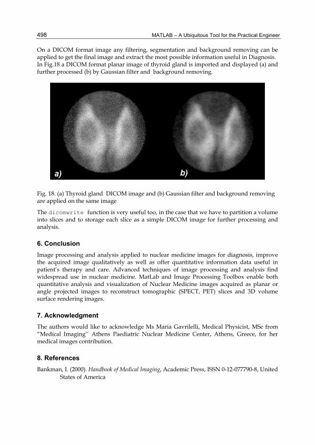
On a DICOM format image any filtering, segmentation and background removing can be applied to get the final image and extract the most possible information useful in Diagnosis. In Fig.18 a DICOM format planar image of thyroid gland is imported and displayed (a) and further processed (b) by Gaussian filter and background removing.

Fig. 18. (a) Thyroid gland DICOM image and (b) Gaussian filter and background removing are applied on the same image

The dicomwrite function is very useful too, in the case that we have to partition a volume into slices and to storage each slice as a simple DICOM image for further processing and analysis.

6. Conclusion Image processing and analysis applied to nuclear medicine images for diagnosis, improve the acquired image qualitatively as well as offer quantitative information data useful in patient’s therapy and care. Advanced techniques of image processing and analysis find widespread use in nuclear medicine. MatLab and Image Processing Toolbox enable both quantitative analysis and visualization of Nuclear Medicine images acquired as planar or angle projected images to reconstruct tomographic (SPECT, PET) slices and 3D volume surface rendering images.

7. Acknowledgment The authors would like to acknowledge Ms Maria Gavrilelli, Medical Physicist, MSc from “Medical Imaging’’ Athens Paediatric Nuclear Medicine Center, Athens, Greece, for her medical images contribution.

8. References Bankman, I. (2000). Handbook of Medical Imaging, Academic Press, ISSN 0-12-077790-8, United

States of America


499

Bidgood, D. & Horii, S. (1992). Introduction to the ACR-NEMA DICOM standard. RadioGraphics, Vol. 12, (May 1992), pp. (345-355)

Delbeke, D.; Coleman, R.E.; Guiberteau M.J.; Brown, M.L.; Royal, H.D.; Siegel, B.A.; Townsend, D.W.; Berland, L.L.; Parker, J.A.; Zubal, G. & Cronin, V. (2006). Procedure Guideline for SPECT/CT Imaging 1.0. The Journal of Nuclear Medicine, Vol. 47, No. 7, (July 2006), pp. (1227-1234).

Gonzalez, R.; Woods, R., & Eddins, S. (2009) Digital Image Processing using MATLAB, (second edition), Gatesmark Publishing, ISBN 9780982085400, United States of America

Lehmann, T.M.; Gönner, C. & Spitzer, K. (1999). Survey: Interpolation Methods in Medical Image Processing. IEEE Transactions on Medical Imaging, Vol.18, No.11, (November 1999), pp. (1049-1075), ISSN S0278-0062(99)10280-5

Lyra, M.; Sotiropoulos, M.; Lagopati, N. & Gavrilleli, M. (2010a). Quantification of Myocardial Perfusion in 3D SPECT images – Stress/Rest volume differences, Imaging Systems and Techniques (IST), 2010 IEEE International Conference on 1-2 July 2010, pp 31 – 35, Thessaloniki, DOI: 10.1109/IST.2010.5548486

Lyra, M.; Striligas, J.; Gavrilleli, M. & Lagopati, N. (2010b). Volume Quantification of I-123 DaTSCAN Imaging by MatLab for the Differentiation and Grading of Parkinsonism and Essential Tremor, International Conference on Science and Social Research, Kuala Lumpur, Malaysia, December 5-7, 2010. http://edas.info/p8295

Li, G. & Miller, R.W. (2010). Volumetric Image Registration of Multi-modality Images of CT, MRI and PET, Biomedical Imaging, Youxin Mao (Ed.), ISBN: 978-953-307-071-1, InTech, Available from:

http://www.intechopen.com/articles/show/title/volumetric-image-registration-of-multi-modality-images-of-ct-mri-and-pet

O’ Gorman, L.; Sammon, M. & Seul M. (2008). Practicals Algorithms for image analysis, (second edition), Cambridge University Press, 978-0-521-88411-2, United States of America

Nailon, W.H. (2010). Texture Analysis Methods for Medical Image Characterisation, Biomedical Imaging, Youxin Mao (Ed.), ISBN: 978-953-307-071-1, InTech, Available from:

http://www.intechopen.com/articles/show/title/texture-analysis-methods-for-medical-image-characterisation

MathWorks Inc. (2009) MATLAB User’s Guide. The MathWorks Inc., United States of America

Perutka K. (2010). Tips and Tricks for Programming in Matlab, Matlab - Modelling, Programming and Simulations, Emilson Pereira Leite (Ed.), ISBN: 978-953-307-125-1, InTech, Available from: http://www.intechopen.com/articles/show/title/tips-and-tricks-for-programming-in-matlab

Toprak, A. & Guler, I. (2006). Suppression of Impulse Noise in Medical Images with the Use of Fuzzy Adaptive Median Filter. Journal of Medical Systems, Vol. 30, (November 2006), pp. (465-471)


500

Wernick, M. & Aarsvold, J. (2004). Emission Tomography: The Fundamentals of PET and SPECT, Elsevier Academic Press, ISBN 0-12-744482-3, China

Wilson, H.B.; Turcotte, L.H. & Halpern, D. (2003). Advanced Mathematics and Mechanics Applications Using MATLAB (third edition), Chapman & Hall/CRC, ISBN 1-58488-262-X, United States of America

Zitova, B. & Flusser J. (2003). Image Registration methods: a survey. Image and Vision Computing. Vol 21, (June 2003), pp. (977-1000)

Date post:	04-Dec-2015
Category:	Documents
Upload:	eko-wahyude
View:	221 times
Download:	0 times

Matlab Tool in NM Image InTech Maria Lyra 2011

Documents