AbstractWe study soliton solutions of matrix Kadomtsev–Petviashvili (KP) equations in atropical limit, in which their support at fixed time is a planar graph and polarizationsare attached to its constituting lines. There is a subclass of “pure line soliton solutions”for which we find that, in this limit, the distribution of polarizations is fully determinedby a Yang–Baxter map. For a vector KP equation, this map is given by an R-matrix,whereas it is a nonlinearmap in the case of amore general matrix KP equation.We alsoconsider the corresponding Korteweg–deVries reduction. Furthermore, exploiting thefine structure of soliton interactions in the tropical limit, we obtain an apparently newsolution of the tetrahedron (or Zamolodchikov) equation. Moreover, a solution of thefunctional tetrahedron equation arises from the parameter dependence of the vectorKP R-matrix.
A line soliton solution of the scalar Kadomtsev–Petviashvili (KP-II) equation (see,e.g., [16]) is, at fixed time t , an exponentially localized wave on a plane. The “tropicallimit” takes it to a piecewise linear structure, a planar graph that represents the wavecrest, with values of the dependent variable attached to its edges. Via the Maslovdequantization formula (also used in “ultra-discretization” [22]), the tropical limit
graph at fixed t can be conveniently computed as the boundary of “dominating phaseregions” in the (xy) plane (see Sect. 4). Applications of this method in the context ofintegrable PDEs can be found in [3,4,6–8,14,19], for example.
In this work, we consider the m × n matrix potential KP equation
where K is a constant n×m matrix and φ anm×n matrix, depending on independentvariables x, y, t , and a subscript indicates a corresponding partial derivative. We willrefer to this equation as pKPK .
If φ is a solution of (1.1), then φR := φK and φL := Kφ solve the ordinarym×m,respectively, n × n, matrix potential KP equation. We also note that, if K = T K ′Swith a constant m′ × m matrix S and a constant n × n′ matrix T , then the m′ × n′matrix φ′ = SφT satisfies the pKPK ′ equation, as a consequence of (1.1).
In the vector case n = 1, writing K = (k1, . . . , km) and φ = (φ1, . . . , φm)ᵀ, (1.1)becomes the following system of coupled equations,
4φi,xt − φi,xxxx − 3φi,yy − 6m∑
j=1
k j((φi,xφ j,x )x − φi,xφ j,y + φi,yφ j,x
) = 0
i = 1, . . . ,m.
By choosing T = 1 and any invertible m × m matrix S that has K as its first row,we have K = K ′S with K ′ = (1, 0, . . . , 0). In terms of the new variable φ′ = Sφ,the above system thus consists of one scalar pKP equation and m − 1 linear equationsinvolving the dependent variable of the former.
For
u := 2φx ,
we obtain from (1.1) the m × n matrix KP equation
( 4 ut − uxxx − 3 (uKu)x )x − 3 uyy + 3
(uK
∫uy dx −
∫uy dx Ku
)
x= 0.
(1.2)
The extension of the scalar KP equation to amatrix version achieves that solitons carryinternal degrees of freedom. The value of the dependent variable along a segmentof the suitably defined (piecewise linear) tropical limit graph will be referred to as“polarization” in the following.
The Korteweg–deVries (KdV) reduction of (1.2) is
4 ut − uxxx − 3 (uKu)x = 0, (1.3)
which we will refer to as KdVK . If K is the identity matrix, this is the matrix KdVequation (see, e.g., [11]). The 2-soliton solution of the latter yields a map from polar-
123
Matrix KP: tropical limit and Yang–Baxter maps
izations at t � 0 to polarizations at t � 0. It is known [12,24] that this yields aYang–Baxter map, i.e., a set-theoretical solution of the (quantum) Yang–Baxter equa-tion (also see [1,23] for the case of the vector Nonlinear Schrödinger equation). Notsurprisingly, this is a feature preserved in the tropical limit. The surprising new insight,however, is that this map governs the evolution of polarizations throughout the tropicallimit graph of a soliton solution. In case of a vector KdV equation, i.e., KdVK withn = 1, it is given by an R-matrix, a linear map solution of the Yang–Baxter equation.
More generally, wewill explore in this work the tropical limit of “pure” (see Sect. 3)soliton solutions of the above K -modified matrix KP equation and demonstrate that aYang–Baxter map governs their structure. There are lots of soliton solutions beyondpure solitons (see, e.g., [16] for the scalar case), but for them a Yang–Baxter map isno longer sufficient to describe the behavior.
In the case of the vector KP equation, the expression for a pure soliton solutioninvolves a function τ which is a τ -function of the scalar KP equation. Its tropical limitat fixed t determines a planar graph, and the vector KP soliton solution associates inthis limit a constant vector (polarization) with each linear segment of the graph. Thepolarization values are then related by a linear Yang–Baxter map, represented by anR-matrix, which does not depend on the independent variables x, y, t , but only on the“spectral parameters” of the soliton solution.
Section 2 summarizes a binary Darboux transformation for the pKPK equation andapplies it to a trivial seed solution in order to obtain soliton solutions. In Sect. 3, werestrict out consideration to the subclass of “pure” soliton solutions. This essentiallydisregards solutions with substructures of the form of Miles resonances. Section 4addresses the tropical limit of pure soliton solutions. The cases of two and three solitonsare then treated in Sects. 5 and 6. Section 7 provides a general proof of the fact that,in the vector case, an R-matrix relates the polarizations at crossings. The linearity ofthe Yang–Baxter map in the vector case is certainly related to the particularly simplestructure of the vector pKP equation mentioned above. In Sect. 8 we show how toconstruct a pure N -soliton solution of the vector KP equation from a pure N -solitonsolution of the scalar KP equation, N vector data and the aforementioned R-matrix.Section 9 extends our exploration of the vector KP 3-soliton case and presents anapparently newsolutionof the tetrahedron (Zamolodchikov) equation (see, e.g., [9] andreferences cited there). In Sect. 10, we reveal the structure of the vector KP R-matrix,which leads us to a more general two-parameter R-matrix. Its parameter dependencedetermines, via a “local” Yang–Baxter equation [18] (also see [9]), a solution of thefunctional tetrahedron equation (see, e.g., [9,15,20]), i.e., the set-theoretical versionof the tetrahedron equation. Finally, Sect. 11 contains some concluding remarks.
2 Soliton solutions of the K -modifiedmatrix KP equation
The following describes a binary Darboux transformation for the pKPK Eq. (1.1). Thisis a simple extension of what is presented in [5], for example. Let φ0 be a solutionof (1.1). Let θ and χ be m × N , respectively, N × n, matrix solutions of the linearequations
123
A. Dimakis, F. Müller-Hoissen
θy = θxx + 2φ0,x K θ θt = θxxx + 3φ0,x K θx + 3
2(φ0,y + φ0,xx )K θ,
χy = −χxx − 2χKφ0,x , χt = χxxx + 3χx Kφ0,x − 3
2χK (φ0,y − φ0,xx ).
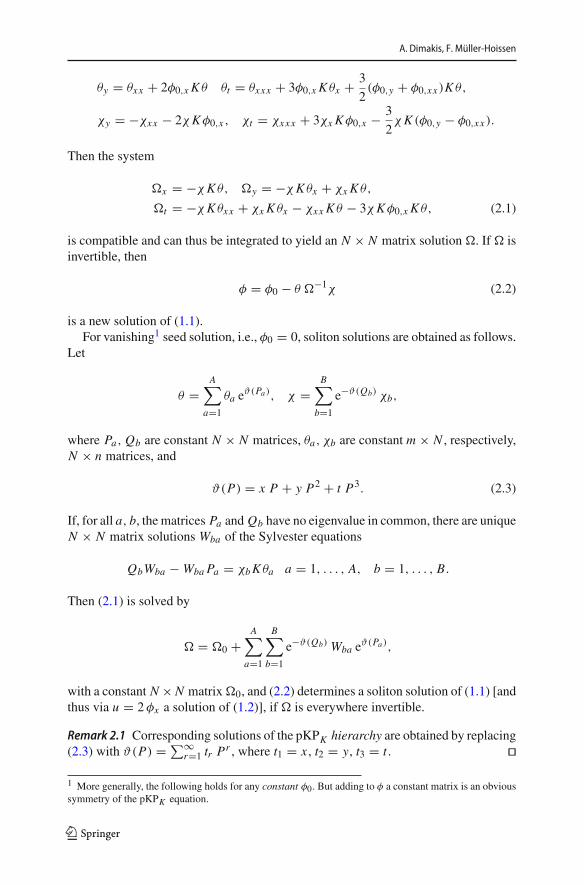
Then the system
�x = −χK θ, �y = −χK θx + χx K θ,
�t = −χK θxx + χx K θx − χxx K θ − 3χKφ0,x K θ, (2.1)
is compatible and can thus be integrated to yield an N × N matrix solution �. If � isinvertible, then
φ = φ0 − θ �−1χ (2.2)
is a new solution of (1.1).For vanishing1 seed solution, i.e., φ0 = 0, soliton solutions are obtained as follows.
Let
θ =A∑
a=1
θa eϑ(Pa), χ =
B∑
b=1
e−ϑ(Qb) χb,
where Pa, Qb are constant N × N matrices, θa, χb are constant m × N , respectively,N × n matrices, and
ϑ(P) = x P + y P2 + t P3. (2.3)
If, for all a, b, the matrices Pa and Qb have no eigenvalue in common, there are uniqueN × N matrix solutions Wba of the Sylvester equations
QbWba − Wba Pa = χbK θa a = 1, . . . , A, b = 1, . . . , B.
Then (2.1) is solved by
� = �0 +A∑
a=1
B∑
b=1
e−ϑ(Qb) Wba eϑ(Pa),
with a constant N ×N matrix�0, and (2.2) determines a soliton solution of (1.1) [andthus via u = 2φx a solution of (1.2)], if � is everywhere invertible.
Remark 2.1 Corresponding solutions of the pKPK hierarchy are obtained by replacing(2.3) with ϑ(P) = ∑∞
r=1 tr Pr , where t1 = x , t2 = y, t3 = t . ��
1 More generally, the following holds for any constant φ0. But adding to φ a constant matrix is an obvioussymmetry of the pKPK equation.
123
Matrix KP: tropical limit and Yang–Baxter maps
3 Pure soliton solutions
In the following, we restrict our considerations to the case where A = B = 1. Thenthere remains only a single Sylvester equation,
Q1W − WP1 = χ1K θ1.
Moreover, we will restrict the matrices P1 and Q1 to be diagonal. It is convenient toname the diagonal entries (“spectral parameters”) in two different ways,
where ξi arem-component column vectors and ηi are n-component row vectors. Thenthe solution of the above Sylvester equation is given by
W = (wi j ), wi j = q j − p j
qi − p jηi K ξ j i, j = 1, . . . , N .
Furthermore, we set �0 = IN , the N × N identity matrix. Hence � = (�i j ) with
�i j = δi j + wi j eϑ(p j )−ϑ(qi ), (3.1)
where δi j is the Kronecker delta. We call soliton solutions obtained from (2.2), withthe above restrictions, “pure solitons”. All what follows refer to them.
We introduce
ϑI :=N∑
i=1
ϑ(pi,ai ) if I = (a1, . . . , aN ) ∈ {1, 2}N .
Instead of using (a1, . . . , aN ) as a subscript (or superscript), we will simply writea1 . . . aN in the following. For example, ϑa1...aN = ϑ(a1,...,aN ).
From (2.2), we find that the pure soliton solutions of the pKPK equation are givenby
φ = F
τ, (3.2)
123
A. Dimakis, F. Müller-Hoissen
with
τ := eϑ2 det�, (3.3)
F := −eϑ2 θ1 eϑ(P1) adj(�) e−ϑ(Q1) χ1, (3.4)
where adj(�) denotes the adjugate of the matrix � and 2 := 2 . . . 2 = (2, . . . , 2).
Proposition 3.1 τ and F have expansions
τ =∑
I∈{1,2}NμI e
ϑI , (3.5)
F =∑
I∈{1,2}NMI e
ϑI , (3.6)
with constants μI and constant m × n matrices MI , where μ2 = 1 and M2 = 0.
Proof From the definition of the determinant, det� = εi1...iN �1i1 · · ·�NiN , with theLevi–Civita symbol εi1...iN and summation convention, we know that det� consistsof a sum of monomials of order N in the entries�i j . Here the latter is given by (3.1). Ifno diagonal term�i i appears in a monomial, its phase factor is eϑ1−ϑ2 . If one diagonalentry �i i = 1 + wi i eϑ(pi,1)−ϑ(pi,2) appears in a monomial, the latter splits into twoparts. Only the part arising from the summand 1 is different as now the phase factor iseϑ1−ϑ2−ϑ(pi,1)+ϑ(pi,2). From monomials containing several diagonal entries of �, weobtain summands with a phase factor of the form
Finally, from a monomial with N diagonal entries of �, we also obtain a constantterm, namely 1. Now our assertion (3.5) follows since τ is det� multiplied by eϑ2 .Clearly, μ2 = 1.
According to the Laplace (cofactor) expansion det� = ∑Nj=1 �i j adj(�) j i with
respect to the i th row, the term �i j adj(�) j i consists of all summands in det�having �i j as a factor. (3.5) implies that a summand of eϑ2adj(�) j i then hasa phase factor of the form eϑI−ϑ(p j,1)+ϑ(pi,2), with some I ∈ {1, 2}N , so thateϑ2 (eϑ(P1) adj(�) e−ϑ(Q1)) j i has the phase factor eϑI . Hence (3.6) holds. Further-more, no entry of eϑ(P1) adj(�) e−ϑ(Q1) is constant, and hence, M2 = 0. ��Remark 3.2 The introduction of the redundant factor eϑ2 in (3.2), via the definitions(3.3) and (3.4), achieves that τ and F are linear combinations of exponentials eϑI ,I ∈ {1, 2}N , in which case we have a very convenient labeling. This is also so if wechoose the factor e−ϑ1 instead, which leads to an expansion in terms of e−ϑI , nowwith M1 = 0. ��
Regularity of a pure soliton solution requires μI ≥ 0 for all I ∈ {1, 2}N (orequivalently μI ≤ 0 for all I ∈ {1, 2}N ) and μI �= 0 for at least one I . If μI = 0 for
123
Matrix KP: tropical limit and Yang–Baxter maps
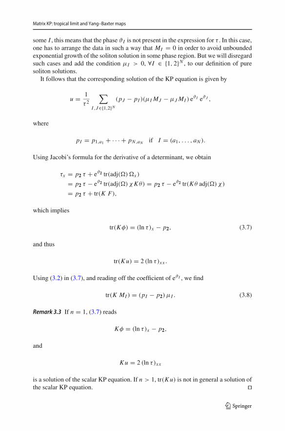
some I , this means that the phase ϑI is not present in the expression for τ . In this case,one has to arrange the data in such a way that MI = 0 in order to avoid unboundedexponential growth of the soliton solution in some phase region. But we will disregardsuch cases and add the condition μI > 0, ∀I ∈ {1, 2}N , to our definition of puresoliton solutions.
It follows that the corresponding solution of the KP equation is given by
u = 1
τ 2
∑
I ,J∈{1,2}N(pJ − pI )(μI MJ − μJ MI ) e
ϑI eϑJ ,
where
pI = p1,a1 + · · · + pN ,aN if I = (a1, . . . , aN ).
Using Jacobi’s formula for the derivative of a determinant, we obtain
Using (3.2) in (3.7), and reading off the coefficient of eϑI , we find
tr(K MI ) = (pI − p2) μI . (3.8)
Remark 3.3 If n = 1, (3.7) reads
Kφ = (ln τ)x − p2,
and
Ku = 2 (ln τ)xx
is a solution of the scalar KP equation. If n > 1, tr(Ku) is not in general a solution ofthe scalar KP equation. ��
123
A. Dimakis, F. Müller-Hoissen
Remark 3.4 Dropping the redundant factor eϑ2 in (3.3) and (3.4) means that we haveto multiply the above expressions (3.5) and (3.6) for τ and F by e−ϑ2 . It is thenevident that φ only depends on differences of phases of the form ϑ(pi,1)−ϑ(pi,2) =(pi,1−pi,2) x+(p2i,1−p2i,2) y+(p3i,1−p3i,2) t . As a consequence, setting pi,2 = −pi,1,i.e.,qi = −pi , eliminates the y terms in all phases. Thismeans that under this conditionfor the parameters, we could have started as well with ϑ(P) = x P + t P3, hencewithout the y term in (2.3). In this way, contact is made with the KdVK reduction inKPK . ��
4 Tropical limit of pure soliton solutions
A crucial point is that we define the tropical limit of the matrix soliton solution viathe tropical limit of the scalar function τ (cf. [6–8]). Let
φI := φ
∣∣∣ϑJ→−∞,J �=I
= MI
μI. (4.1)
In a region where a phase ϑI dominates all others, in the sense that log(μI eϑI ) >
log(μJ eϑJ ) for all participating J �= I , the tropical limit of the potential φ is givenby (4.1). It should be noticed that these expressions do not depend on the coordinatesx, y, t .
The boundary between the regions associated with the phases ϑI and ϑJ is deter-mined by the condition
μI eϑI = μJ e
ϑJ . (4.2)
Not all parts of such a boundary are visible at fixed time, since some of themmay lie ina region where a third phase dominates the two phases. The tropical limit of a solitonsolution at a fixed time t has support on the visible parts of the boundaries between theregions associated with phases appearing in τ . On such a visible boundary segment,the value of u is given by
uI J = 1
2(pI − pJ ) (φI − φJ ) .
For I = (a1, . . . , aN ) we set
Ik(a) = (a1, . . . , ak−1, a, ak+1, . . . , aN ).
At fixed time, the set of line segments associated with the kth soliton are obtainedfrom (4.2) with I = Ik(1) and J = Ik(2), for all possible I . They satisfy
(pk,2 − pk,1) x + (p2k,2 − p2k,1) y + (p3k,2 − p3k,1) t + lnμIk (2)
μIk (1)= 0. (4.3)
123
Matrix KP: tropical limit and Yang–Baxter maps
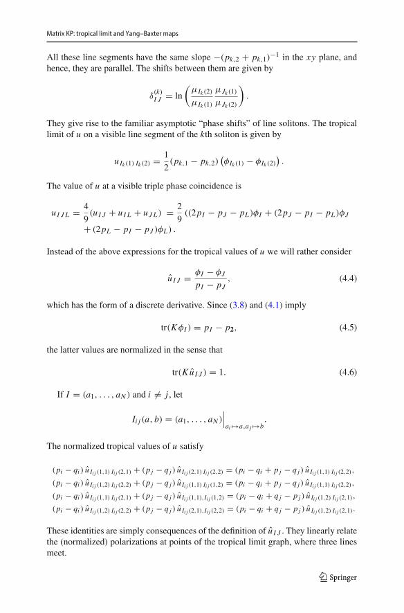
All these line segments have the same slope −(pk,2 + pk,1)−1 in the xy plane, andhence, they are parallel. The shifts between them are given by
δ(k)I J = ln
(μIk (2)
μIk (1)
μJk (1)
μJk (2)
).
They give rise to the familiar asymptotic “phase shifts” of line solitons. The tropicallimit of u on a visible line segment of the kth soliton is given by
uIk (1) Ik (2) = 1
2(pk,1 − pk,2)
(φIk (1) − φIk (2)
).
The value of u at a visible triple phase coincidence is
uI J L = 4
9(uI J + uI L + uJ L) = 2
9((2pI − pJ − pL)φI + (2pJ − pI − pL)φJ
+ (2pL − pI − pJ )φL) .
Instead of the above expressions for the tropical values of u we will rather consider
u I J = φI − φJ
pI − pJ, (4.4)
which has the form of a discrete derivative. Since (3.8) and (4.1) imply
tr(KφI ) = pI − p2, (4.5)
the latter values are normalized in the sense that
tr(Ku I J ) = 1. (4.6)
If I = (a1, . . . , aN ) and i �= j , let
Ii j (a, b) = (a1, . . . , aN )
∣∣∣ai �→a,a j �→b
.
The normalized tropical values of u satisfy
(pi − qi ) u Ii j (1,1) Ii j (2,1) + (p j − q j ) u Ii j (2,1) Ii j (2,2) = (pi − qi + p j − q j ) u Ii j (1,1) Ii j (2,2),
(pi − qi ) u Ii j (1,2) Ii j (2,2) + (p j − q j ) u Ii j (1,1) Ii j (1,2) = (pi − qi + p j − q j ) u Ii j (1,1) Ii j (2,2),
(pi − qi ) u Ii j (1,1) Ii j (2,1) + (p j − q j ) u Ii j (1,1),Ii j (1,2) = (pi − qi + q j − p j ) u Ii j (1,2) Ii j (2,1),
(pi − qi ) u Ii j (1,2) Ii j (2,2) + (p j − q j ) u Ii j (2,1),Ii j (2,2) = (pi − qi + q j − p j ) u Ii j (1,2) Ii j (2,1).
These identities are simply consequences of the definition of u I J . They linearly relatethe (normalized) polarizations at points of the tropical limit graph, where three linesmeet.
The tropical values of the pKPK solution φ in the dominant phase regions are thengiven by
φ11 = (q1 − p1)(q2 − p2)
α κ11 κ22
(κ22
p2 − q2ξ1 ⊗ η1 + κ11
p1 − q1ξ2 ⊗ η2
+ κ12
q1 − p2ξ1 ⊗ η2 + κ21
q2 − p1ξ2 ⊗ η1
),
φ12 = (p1 − q1)ξ1 ⊗ η1
κ11, φ21 = (p2 − q2)
ξ2 ⊗ η2
κ22, φ22 = 0.
Remark 5.1 The above values φab solve the following nonlinear equation,
(1 + tr
K (φ12 − φ22)K (φ21 − φ22)
(q1 − p2)(p1 − q2)
)(φ11 − φ22) − (φ12 − φ22)K (φ21 − φ22)
q1 − p2
+ (φ21 − φ22)K (φ12 − φ22)
p1 − q2− (φ12 − φ22) − (φ21 − φ22) = 0. (5.1)
Addressing more than two solitons, nonzero counterparts of φ22 will show up, asdisplayed in this equation. ��
For the tropical values of u along the phase region boundaries, we obtain
u1,in := u11,21 = α−1(1m − q2 − p2
q2 − p1
ξ2 ⊗ η2
κ22K
)ξ1 ⊗ η1
κ11
(1n − q2 − p2
q1 − p2K
ξ2 ⊗ η2
κ22
),
u2,in := u21,22 = ξ2 ⊗ η2
κ22,
u1,out := u12,22 = ξ1 ⊗ η1
κ11,
123
Matrix KP: tropical limit and Yang–Baxter maps
u2,out := u11,12 = α−1(1m − q1 − p1
q1 − p2
ξ1 ⊗ η1
κ11K
)ξ2 ⊗ η2
κ22
(1n − q1 − p1
q2 − p1K
ξ1 ⊗ η1
κ11
),
(5.2)
where 1m stands for the m ×m identity matrix. For the in/out classification, see Fig. 1below. All the matrices in (5.2) have rank one, which is not at all obvious from theform of φab. We obtain the following nonlinear relation between “incoming” and“outgoing” polarizations,
u1,out = α−1in
(1m − q2 − p2
p1 − p2u2,inK
)u1,in
(1n − p2 − q2
q1 − q2Ku2,in
),
u2,out = α−1in
(1m − q1 − p1
q1 − q2u1,inK
)u2,in
(1n − p1 − q1
p1 − p2Ku1,in
), (5.3)
where
αin = 1 − (p1 − q1)(p2 − q2)
(p1 − p2)(q1 − q2)tr
(Ku1,inKu2,in
).
We note that α αin = 1. (5.3) determines a new nonlinear Yang–Baxter map
R : (u1,in, u2,in) �→ (u1,out, u2,out), (5.4)
with parameters pi , qi , i = 1, 2.We verified directly that this satisfies theYang–Baxterequation
R12 ◦ R13 ◦ R23 = R23 ◦ R13 ◦ R12, (5.5)
where the subscripts indicate on which two factors of a threefold Cartesian productthe mapR acts. An explanation why the Yang–Baxter equation holds will be providedin Sect. 6.
Writing
ua,in = ξa,in ⊗ ηa,in
ηa,inK ξa,in, ua,out = ξa,out ⊗ ηa,out
ηa,outK ξa,outa = 1, 2,
determines ξ1,in/out and η1,in/out up to scalings. We find
ξ1,out = α−1/2in
(1m − p2 − q2
p2 − p1
ξ2,in ⊗ η2,in
η2,inK ξ2,inK
)ξ1,in,
ξ2,out = α−1/2in
(1m − q1 − p1
q1 − q2
ξ1,in ⊗ η1,in
η1,inK ξ1,inK
)ξ2,in,
η1,out = α−1/2in η1,in
(1n − q2 − p2
q2 − q1K
ξ2,in ⊗ η2,in
η2,inK ξ2,in
),
123
A. Dimakis, F. Müller-Hoissen
Fig. 1 The first is a contour plot of tr(Ku) = 2(ln τ)xx for a 2-soliton solution of the 2 × 3 matrix KPequation, at t = 0 in the xy plane, using the data of Example 5.3. Viewed as a process in y direction, theYB map takes the values of the KP variable on the lower two legs to those on the upper two. A numberi j indicates the respective dominating phase region. In the second plot, the value of p2 is replaced by−1/4+ 10−5, so that p2 is very close to q1. Here, a boundary segment between phase regions 11 and 22 isvisible. The third plot presents an example, where the parameters of the 2-soliton solution are now chosensuch that the latter boundary is hidden and instead a boundary segment between phase regions 12 and 21 isvisible
Remark 5.2 In (5.2), we found that u2,in and u1,out have a simple elementary form.They are the polarizations at the two boundary lines of the dominating phase regionnumbered by 22 = (2, 2), see Fig. 1. We know from Proposition 3.1 that it is specialsince M22 = 0. Considering an “evolution” in negative x direction (instead of ydirection), thus, offers a more direct derivation of the Yang–Baxter map. ��Example 5.3 Let m = 3 and n = 2. Choosing
p1 = −3/4, p2 = 1/4, q1 = −1/4, q2 = 3/4,
and
η1 = (1, 0), η2 = (0, 1), ξ1 =⎛
⎝2/35
−2
⎞
⎠ , ξ2 =⎛
⎝12/32
⎞
⎠ , K =(1 1 11 2 1
),
we obtain the first contour plot, at t = 0, shown in Fig. 1. Figure 2 shows plots of thecomponents of the transpose of u. Choosing instead p2 close to q1 reveals an “innerstructure” of crossings, see the second plot in Fig. 1. This is the (phase) shift mentionedin Sect. 4. ��
123
Matrix KP: tropical limit and Yang–Baxter maps
Fig. 2 Plot of the six components of the transpose of u at t = 0 for the solution of the 3 × 2 matrix KPequation with the (first) data specified in Example 5.3. The components are localized exactly where tr(Ku)
is localized, cf. Fig. 1
Remark 5.4 Weshould stress that the relevant structures are actually three-dimensionaland our figures only display a two-dimensional cross section. Instead of displayingstructures in the xy plane at constant t , we may as well look at those in the xt planeat constant y. The latter becomes relevant if we consider the KdVK reduction. ��Remark 5.5 Soliton solutions of KdVK are obtained from those of KPK by settingqi = −pi , i = 1, . . . , N , see Remark 3.4. Then the above equations reduce to
ξ1,out = α−1/2in
(1m − 2p2
p2 − p1
ξ2,in ⊗ η2,in
η2,inK ξ2,inK
)ξ1,in,
ξ2,out = α−1/2in
(1m − 2p1
p1 − p2
ξ1,in ⊗ η1,in
η1,inK ξ1,inK
)ξ2,in,
η1,out = α−1/2in η1,in
(1n − 2p2
p2 − p1K
ξ2,in ⊗ η2,in
η2,inK ξ2,in
),
η2,out = α−1/2in η2,in
(1n − 2p1
p1 − p2K
ξ1,in ⊗ η1,in
η1,inK ξ1,in
),
with
αin = 1 + 4p1 p2(p1 − p2)2
η1,inK ξ2,in η2,inK ξ1,in
η1,inK ξ1,in η2,inK ξ2,in.
If K is the N × N identity matrix, this becomes the Yang–Baxter map first found byVeselov [24], also see [12,21]. The factor α
−1/2in is missing in these publications, but
such a factor is necessary for the map to satisfy the Yang–Baxter equation. It shouldbe noticed that Veselov’s “Lax pair” [24] only determines the Yang–Baxter map upto a factor, but such a factor has to be chosen appropriately in order to satisfy theYang–Baxter equation. One can avoid the square root in the above expression at theprice of having an asymmetric appearance of factors α−1
in . ��
123
A. Dimakis, F. Müller-Hoissen
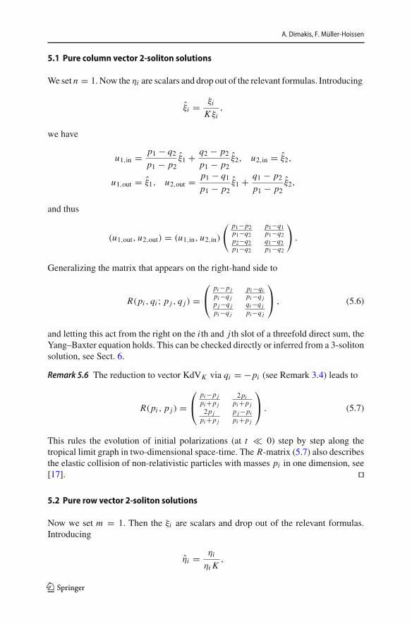
5.1 Pure column vector 2-soliton solutions
We set n = 1. Now the ηi are scalars and drop out of the relevant formulas. Introducing
ξi = ξi
K ξi,
we have
u1,in = p1 − q2p1 − p2
ξ1 + q2 − p2p1 − p2
ξ2, u2,in = ξ2,
u1,out = ξ1, u2,out = p1 − q1p1 − p2
ξ1 + q1 − p2p1 − p2
ξ2,
and thus
(u1,out, u2,out) = (u1,in, u2,in)
( p1−p2p1−q2
p1−q1p1−q2
p2−q2p1−q2
q1−q2p1−q2
).
Generalizing the matrix that appears on the right-hand side to
R(pi , qi ; p j , q j ) =⎛
⎝pi−p jpi−q j
pi−qipi−q j
p j−q jpi−q j
qi−q jpi−q j
⎞
⎠ , (5.6)
and letting this act from the right on the i th and j th slot of a threefold direct sum, theYang–Baxter equation holds. This can be checked directly or inferred from a 3-solitonsolution, see Sect. 6.
Remark 5.6 The reduction to vector KdVK via qi = −pi (see Remark 3.4) leads to
R(pi , p j ) =⎛
⎝pi−p jpi+p j
2pipi+p j
2p jpi+p j
p j−pipi+p j
⎞
⎠ . (5.7)
This rules the evolution of initial polarizations (at t � 0) step by step along thetropical limit graph in two-dimensional space-time. The R-matrix (5.7) also describesthe elastic collision of non-relativistic particles with masses pi in one dimension, see[17]. ��
5.2 Pure row vector 2-soliton solutions
Now we set m = 1. Then the ξi are scalars and drop out of the relevant formulas.Introducing
ηi = ηi
ηi K,
123
Matrix KP: tropical limit and Yang–Baxter maps
we have
u1,in = q1 − p2q1 − q2
η1 + p2 − q2q1 − q2
η2, u2,in = η2,
u1,out = η1, u2,out = q1 − p1q1 − q2
η1 + p1 − q2q1 − q2
η2,
so that
(u1,outu2,out
)=
( q2−q1p2−q1
p2−q2p2−q1
p1−q1p2−q1
p2−p1p2−q1
)(u1,inu2,in
),
which determines a Yang–Baxter map. Let
R(pi , qi ; p j , q j ) :=⎛
⎝q j−qip j−qi
p j−q jp j−qi
pi−qip j−qi
p j−pip j−qi
⎞
⎠
act on the i th and j th slot of a direct sum. Then the Yang–Baxter equation holds. Wenote that R(pi , qi ; p j , q j ) = R(qi , pi ; q j , p j )
Note that αi j = αi j j . Recall that the coefficient of eϑabc in the expression for τ ,respectively, F , has been named μabc, respectively, Mabc. The tropical value in theregion where ϑabc dominates all other phases is given by
φabc = Mabc
μabc.
The corresponding values can be read off from (6.1) and (6.2).The Yang–Baxter property of the nonlinear map (5.4) can be deduced from the
pure 3-soliton solution in the following way. Numbering the (in y direction) incomingsolitons by 1, 2, 3 in x direction, for t � 0 first (according to increasing values ofy) solitons 1 and 2 interact, then solitons 1 and 3, and finally solitons 2 and 3. Fort � 0 solitons 2 and 3 meet first, then solitons 1 and 3, and finally solitons 1 and 2.Also see Fig. 3 below. Recalling that the polarizations along the tropical limit graphdo not depend on the variables x, y, t , this implies that in both cases we obtain thesame outgoing polarizations. Hence, the Yang–Baxter equation (5.5) holds. This isworked out in detail only for the simpler vector KP case in the next subsection. Butwe checked the general case as well.
That we can check the Yang–Baxter equation in this way is because of the factthat, in the tropical limit and at fixed t , we have well-defined interaction points ofsolitons. In the original wave description, we can only compute the asymptotics, i.e.,
123
Matrix KP: tropical limit and Yang–Baxter maps
Fig. 3 Yang–Baxter relation in terms of vector KP line solitons. These are contour plots in the xy plane(horizontal x- and vertical y-axis) of a 3-soliton solution at negative, respectively, positive t . A number abcindicates the respective dominating phase region
the structure of incoming and outgoing solitons, but we have no description of whathappens in the interaction region.
Because of the exponential localization of waves, a pure N -soliton solution, N > 2,looks like a 2-soliton solution close enough to a crossing in the tropical limit graph.This becomes exact in the tropical limit. It implies that the Yang–Baxter map (5.4)acts at any crossing of the tropical limit graph. We will discuss this in more detail forthe vector KP case in Sect. 7.
6.1 Pure vector KP 3-soliton solutions
Now we restrict our considerations to the vector case n = 1. Using
ξi = ξi
K ξi,
we obtain
u122,222 = ξ1, u212,222 = ξ2, u221,222 = ξ3,
u111,211 = (p1 − q2)(p1 − q3)
(p1 − p2)(p1 − p3)ξ1 − (p2 − q2)(p2 − q3)
(p1 − p2)(p2 − p3)ξ2 + (p3 − q2)(p3 − q3)
(p1 − p3)(p2 − p3)ξ3,
u111,121 = (p1 − q1)(p1 − q3)
(p1 − p2)(p1 − p3)ξ1 − (p2 − q1)(p2 − q3)
(p1 − p2)(p2 − p3)ξ2 + (p3 − q1)(p3 − q3)
(p2 − p3)(p1 − p3)ξ3,
u111,112 = (p1 − q1)(p1 − q2)
(p1 − p2)(p1 − p3)ξ1 − (p2 − q1)(p2 − q2)
(p1 − p2)(p2 − p3)ξ2 + (p3 − q1)(p3 − q2)
(p1 − p3)(p2 − p3)ξ3,
u121,221 = p1 − q3p1 − p3
ξ1 − p3 − q3p1 − p3
ξ3, u121,122 = p1 − q1p1 − p3
ξ1 − p3 − q1p1 − p3
ξ3,
u112,122 = p1 − q1p1 − p2
ξ1 − p2 − q1p1 − p2
ξ2, u211,221 = p2 − q3p2 − p3
ξ2 − p3 − q3p2 − p3
ξ3,
u211,212 = p2 − q2p2 − p3
ξ2 − p3 − q2p2 − p3
ξ3, u112,212 = p1 − q2p1 − p2
ξ1 − p2 − q2p1 − p2
ξ2.
123
A. Dimakis, F. Müller-Hoissen
The contour plots in Fig. 3 show the structure at fixed t with t < 0 and t > 0,respectively. The lines extending to the bottomare numberedby1, 2, 3 from left to right(displayed as blue, red, green, respectively). Thinking of three particles undergoing ascattering process in y direction, they carry polarizations that change at crossings. Asy increases we have
for t > 0. The numbers i j assigned to the steps refer to the “particles” involved. Inboth cases, we start and end with the same vectors, and this implies the Yang–Baxterequation for the associated transformations. Let Va1a2a3,b1b2b3 be the column vectorformed by the coefficients of ua1a2a3,b1b2b3 with respect to ξ1, ξ2, ξ3. The followingmatrices are composed of these column vectors,
U123 = (V111,211 V211,221 V221,222
), U213 = (
V121,221 V111,121 V221,222),
U231 = (V122,222 V111,121 V121,122
), U321 = (
V122,222 V112,122 V111,112),
U132 = (V111,211 V212,222 V211,212
), U312 = (
V112,212 V212,222 V111,112).
They represent the triplets of polarizations constituting the above chains. Next wedefine matrices
r12 = U−1123U213 = U−1
312U321, r13 = U−1213U231 = U−1
132U312,
r23 = U−1231U321 = U−1
123U132,
which turn out to be given in terms of the R-matrix (5.6). For example,
r13 =
⎛
⎜⎜⎝
p1−p3p1−q3
0 p1−q1p1−q3
0 1 0p3−q3p1−q3
0 q1−q3p1−q3
⎞
⎟⎟⎠ .
The Yang–Baxter equation reads
r12 r13 r23 = r23 r13 r12.
Figure 4 shows plots of Ku for a choice of the parameters.
123
Matrix KP: tropical limit and Yang–Baxter maps
Fig. 4 Plots of the scalar Ku for a “Yang–Baxter line soliton configuration” of a vector KP equation attimes t < 0, t = 0 and t > 0
6.2 Vector KdV 3-soliton solutions
We impose the KdV reduction, see Remark 3.4, and replace (2.3) by
ϑ(P) = x P + t P3 + s P5.
The additional last term introduces the next evolution variable s of the KdV hierarchy,also see Remark 2.1.
Let us consider, for simplicity, the KdVK equation with m = 3 and K = (1, 1, 1),and the special solution with parameters
θ1 = I3, χ1 = (1,− 1, 1)ᵀ.
The tropical limit graph is displayed in Fig. 5 for p1 = 1/2, p2 = 3/4, p3 = 1, anddifferent values of s. We have the matrix
U123 = (u111,211 u211,221 u221,222
) =
⎛
⎜⎜⎝
(p1+p2)(p1+p3)(p1−p2)(p1−p3)
0 0
− 2p2(p2+p3)(p1−p2)(p2−p3)
p2+p3p2−p3
02p3(p2+p3)
(p1−p3)(p2−p3)− 2p3
p2−p31
⎞
⎟⎟⎠
Fig. 5 Tropical limit graph and dominating phase regions of a vector KdV solution in two-dimensionalspace-time (x horizontal, t vertical), at s = − 10, s = 0 and s = 10. See Sect. 6.2. Numbers 1, 2, 3 (in red)attached to lines identify appearances of the respective soliton. Here bounded lines are formally associatedwith a pair of a (virtual) anti-soliton, indicated by a bar over the respective number, and a (virtual) soliton.At s = 0, a “composite” of three virtual solitons (123) shows up (color figure online)
123
A. Dimakis, F. Müller-Hoissen
of initial polarizations. The next values uabc,de f are then obtained by application ofthe R-matrix (5.7) from the right, and so forth, following either the left or the rightgraph in Fig. 5 in upwards (i.e., t) direction. Since the initial and the final polarizationsare the same, the Yang–Baxter equation holds. Here the R-matrix describes the timeevolution of polarizations in the tropical limit.
Figure 5 suggests to think of R-matrices as being associated with bounded lines,which may be thought of as representing “virtual solitons”. Interaction of two solitonsthen means exchange of a virtual soliton, frequently called a “resonance”.
At s = 0, see the plot in the middle of Fig. 5, something peculiar occurs, namely asort of three-particle interaction. This is a degenerate special case to which the Yang–Baxter description does not apply. To be precise, the statement that the Yang–Baxtermap rules the polarizations along the tropical limit graph thus holds for s �= 0.
Tounderstandwhat thismeans, let usmore generally think of any system, dependingcontinuously on a parameter, say s, and carrying a structure, which is described by amap such that the left-hand side of the Yang–Baxter equation is realized for s < 0,and the right-hand side for s > 0. Then there is a “transition point”, s = 0, where theYang–Baxter equation does not apply. The system is actually more complete, sinceit also contains a transition structure. The latter, however, cannot be resolved into asequence of three applications of a map. This is the situation we meet in the tropicallimit analysis of pure KP multi-soliton solutions. There are isolated parameter values,corresponding to “transitions”, at which the Yang–Baxter equation does not apply.
7 Tropical limit of pure vector solitons and the R-matrix
We set n = 1 (vector case). The following results describe what happens at a crossingof two solitons, numbered by i and j , depicted as a contour plot in Fig. 6.
Proof This is quickly verified for the 2-soliton solution (N = 2). But at a crossing, ageneral solution φ is equivalent to a 2-soliton solution, since there the four elementary
Fig. 6 A crossing of solitonswith numbers i and j at fixedtime in the xy plane, and thenumbers of the four phases thatare involved
123
Matrix KP: tropical limit and Yang–Baxter maps
phases ϑ(pi,a), ϑ(p j,a), a = 1, 2, dominate all others, and hence, the exponential ofany other phase vanishes in the tropical limit. ��Remark 7.2 (7.1) can be regarded as a vector version of a scalar linear quadrilateralequation, satisfying “consistency on a cube”, see (15) in [2]. Such a linear relationdoes not hold in the matrix case where m, n > 1. But (5.1), with φab replaced byφIi j (a,b) (in which case we have φIi j (2,2) �= 0, in general) is a nonlinear counterpart of(7.1). The latter can be deduced from it for n = 1 by using (4.5). ��Theorem 7.3
(u Ii j (1,1),Ii j (2,1) u Ii j (2,1),Ii j (2,2)
)R(pi , qi ; p j , q j ) = (
u Ii j (1,2),Ii j (2,2) u Ii j (1,1),Ii j (1,2))
(7.2)
with
R(pi , qi ; p j , q j ) =( pi−p j
pi−q j
pi−qipi−q j
p j−q jpi−q j
qi−q jpi−q j
).
Proof Using (4.4) we can directly verify that the following relations hold as a conse-quence of (7.1),
pi − p j
pi − q ju Ii j (1,1),Ii j (2,1) + p j − q j
pi − q ju Ii j (2,1),Ii j (2,2) = u Ii j (1,2),Ii j (2,2),
pi − qipi − q j
u Ii j (1,1),Ii j (2,1) + qi − q j
pi − q ju Ii j (2,1),Ii j (2,2) = u Ii j (1,1),Ii j (1,2).
In matrix form, this is (7.2). ��We already know that R(pi , qi ; p j , q j ) satisfies the Yang–Baxter equation.
8 Construction of pure vector KP soliton solutions from a scalar KPsolution and the R-matrix
Given a τ -function for a pure N -soliton solution of the scalar KP equation, the Yang–Baxter R-matrix found above can be used to construct a pure N -soliton solution ofthe vector KP equation. We will explain this for the case N = 3.
The τ -function of the pure 3-soliton solution of the scalar KP-II equation is givenby
as obtained by the Wronskian method (see, e.g., [13]). Comparison with (3.5) showsthat μI = �I .
123
A. Dimakis, F. Müller-Hoissen
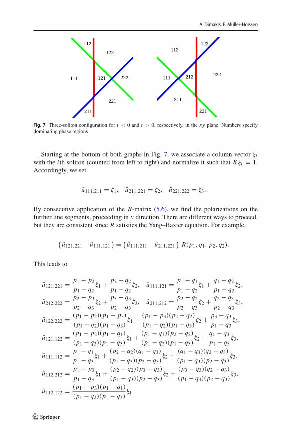
Fig. 7 Three-soliton configuration for t < 0 and t > 0, respectively, in the xy plane. Numbers specifydominating phase regions
Starting at the bottom of both graphs in Fig. 7, we associate a column vector ξiwith the i th soliton (counted from left to right) and normalize it such that K ξi = 1.Accordingly, we set
u111,211 = ξ1, u211,221 = ξ2, u221,222 = ξ3.
By consecutive application of the R-matrix (5.6), we find the polarizations on thefurther line segments, proceeding in y direction. There are different ways to proceed,but they are consistent since R satisfies the Yang–Baxter equation. For example,
From (4.1) we can read off Mabc and thus obtain via (3.2) and (3.4) the solution
φ = 1
τ
2∑
a,b,c=1
Mabc eϑabc
of the vector pKP equation. This procedure can easily be applied to a larger numberof solitons.
Remark 8.1 The construction described in this section cannot be extended to thematrixKP case, since then the function τ does not correspond to a solution of the scalar KPequation, or of any other meaningful equation.
9 A solution of the tetrahedron equation
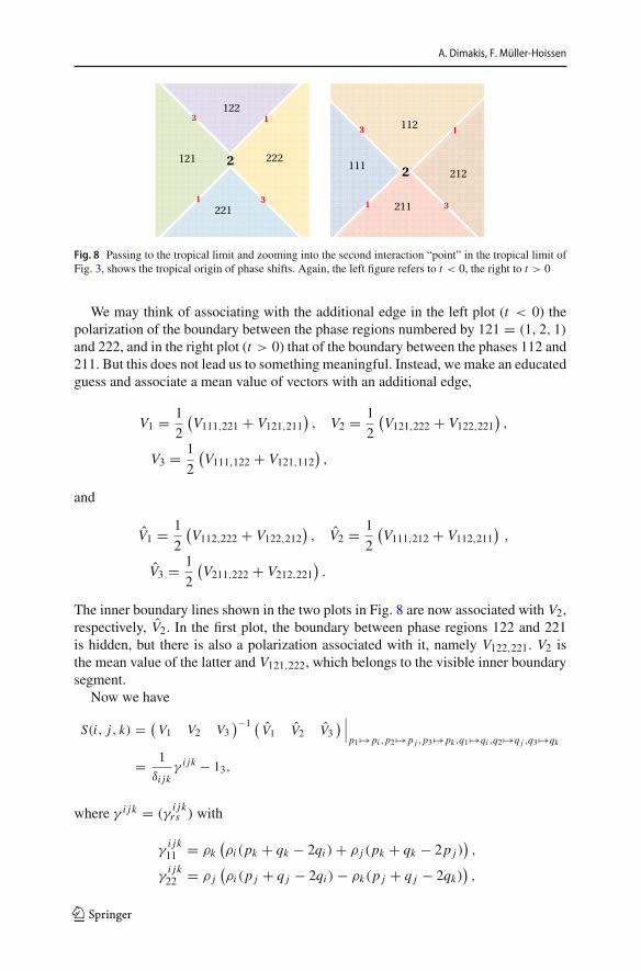
In this section, we address again the case of three pure solitons, see Sect. 6. Becauseof the occurrence of phase shifts, in the tropical limit a crossing of two solitons doesnot really take place in a point. Figure 8 shows this for the second interaction (in thevertical y direction) in Fig. 3, or Fig. 7.
123
A. Dimakis, F. Müller-Hoissen
Fig. 8 Passing to the tropical limit and zooming into the second interaction “point” in the tropical limit ofFig. 3, shows the tropical origin of phase shifts. Again, the left figure refers to t < 0, the right to t > 0
We may think of associating with the additional edge in the left plot (t < 0) thepolarization of the boundary between the phase regions numbered by 121 = (1, 2, 1)and 222, and in the right plot (t > 0) that of the boundary between the phases 112 and211. But this does not lead us to something meaningful. Instead, we make an educatedguess and associate a mean value of vectors with an additional edge,
V1 = 1
2
(V111,221 + V121,211
), V2 = 1
2
(V121,222 + V122,221
),
V3 = 1
2
(V111,122 + V121,112
),
and
V1 = 1
2
(V112,222 + V122,212
), V2 = 1
2
(V111,212 + V112,211
),
V3 = 1
2
(V211,222 + V212,221
).
The inner boundary lines shown in the two plots in Fig. 8 are now associated with V2,respectively, V2. In the first plot, the boundary between phase regions 122 and 221is hidden, but there is also a polarization associated with it, namely V122,221. V2 isthe mean value of the latter and V121,222, which belongs to the visible inner boundarysegment.
We verified that this constitutes a (to our knowledge new) solution of the tetrahedron(Zamolodchikov) equation (see, e.g., [9] and references cited there)
R123R145R246R356 = R356R246R145R123. (9.1)
An explanation for the choices of numbers in the above definition of Rαβγ can befound in Fig. 9. Also see [15].
Remark 9.1 The KdVK reduction qi = −pi yields
SKdV(i, j, k) =
⎛
⎜⎜⎜⎝
− (pi+pk )(p j−pk )(pi−pk )(p j+pk )
2(pi−p j )pk(pi−pk )(p j+pk )
2(pi−p j )pk(pi−pk )(p j+pk )
2p j (pi+pk )(pi+p j )(p j+pk )
(pi−p j )(p j−pk )(pi+p j )(p j+pk )
2p j (pi+pk )(pi+p j )(p j+pk )
2pi (p j−pk )(pi+p j )(pi−pk )
2pi (p j−pk )(pi+p j )(pi−pk )
− (pi−p j )(pi+pk )(pi+p j )(pi−pk )
⎞
⎟⎟⎟⎠ ,
which determines a simpler solution of the tetrahedron equation. ��
123
A. Dimakis, F. Müller-Hoissen
Fig. 9 KP line solitons remain parallel while moving. The two chains of line configurations (here shiftsare disregarded) show the two different ways in which a 4-soliton solution can evolve from the same initialto the same final configuration. (The two chains represent the higher Bruhat order B(4, 2), cf. [9].) Thisimplies the tetrahedron equation. Here (red) numbers attached to lines enumerate the four solitons. Also thecrossings of pairs of them are enumerated (by numbers in black). Time evolution proceeds by inversion oftriangles. In the first chain, the first step is the inversion of the triangle formed by the crossings numbered1, 2, 3. The second step is the inversion of the triangle formed by the crossings 1, 4, 5. The latter involvesthe solitons with numbers 1, 2, 4 (color figure online)
10 A generalization of the vector KP R-matrix and a solution of thefunctional tetrahedron equation
The vector KdV R-matrix (5.7) is obtained from the one-parameter R-matrix (see,e.g., [15,20] for a similar R-matrix)
R(x) =(
x 1 + x1 − x −x
),
by setting x = (p1 − p2)/(p1 + p2). The local Yang–Baxter equation
R12(x) R13(y) R23(z) = R23(Z) R13(Y ) R12(X),
where indices αβ indicate on which components of a threefold direct sum R acts,determines the map (x, y, z) �→ (X ,Y , Z) given by
X = xy
x + z − xyz, Y = x + z − xyz, Z = yz
x + z − xyz.
A similar map appeared in [15,20]. A general argument (cf., e.g., [9] and referencescited there) implies that
R(x, y, z) := (X ,Y , Z)
solves the (functional) tetrahedron equation (9.1), where a “product” of R’s now hasto be interpreted as composition of maps. This tetrahedron map is involutive. Settingx = (p1 − p2)/(p1 + p2), y = (p1 − p3)/(p1 + p3) and z = (p2 − p3)/(p2 + p3),it becomes the identity.
123
Matrix KP: tropical limit and Yang–Baxter maps
Correspondingly, the vector KP R-matrix (5.6) is obtained from the more generaltwo-parameter R-matrix
R(x, y) =(
x y1 − x 1 − y
),
by setting x = (p1 − p2)/(p1 − q2) and y = (p1 − q1)/(p1 − q2). The local Yang–Baxter equation
determines the map (x, y; z, u; v,w) �→ (X ,Y ; Z ,U ; V ,W ), where
X = z C, Y =(z − A
x
)C, Z = x
C,
U = 1 − B, V = vz (x − y)
A, W = 1 − (1 − u)(1 − w)
B,
with
A = uvx − ux − vy + xz, B = uwx − ux − wy + 1,
C = AB − A(1 − u)(1 − w)x − Bv (x − y)
AB − A(1 − u)(1 − w) − Bvz (x − y).
Then
R(x, y; z, u; v,w) := (X ,Y ; Z ,U ; V ,W )
solves the functional (i.e., set-theoretical) tetrahedron equation.
11 Conclusions
In this work, we explored “pure” soliton solutions of matrix KP equations in a trop-ical limit. In case of the reduction to matrix KdV, this consists of a planar graph in(two-dimensional) space-time, with polarizations assigned to its edges. Given initialpolarizations, the evolution of them along the graph is ruled by a Yang–Baxter map.For the vector KdV equation, this is a linear map, hence an R matrix. The classicalscattering process of matrix KdV solitons resembles in the tropical limit the scatter-ing of point particles in a 2-dimensional integrable quantum field theory, which ischaracterized by a scattering matrix that solves the (quantum) Yang–Baxter equation.
We have shown that all this holds more generally for KPK , where the tropical limitat a fixed time t is given by a graph in the xy plane, with polarizations attached tothe soliton lines. Moreover, the vector KP case provides us with a realization of the“classical straight-string model” considered in [15]. It should be noticed, however,
123
A. Dimakis, F. Müller-Hoissen
that KP line solitons in the tropical limit are not, in general, straight because of theappearance of (phase) shifts.
As a side product of our explorations of the tropical limit of pure vector KP solitons,we derived apparently new solutions of the tetrahedron (Zamolodchikov) equation.Whether these solutions are relevant, e.g., for the construction of solvable models ofstatistical mechanics in three dimensions, has still to be seen.
Another subclass of soliton solutions of the vector KP equation consists of those,for which the support at fixed time is a rooted and generically binary tree in the tropicallimit. For the scalar KP equation, this has been extensively explored in [6,7]. Instead ofthe Yang–Baxter equation, the pentagon equation (see [9] and references therein) nowplays a role in governing corresponding vector solitons. This is treated in a separatework [10].
Acknowledgements Open access funding provided by Max Planck Society. A.D. thanks V. Papageorgioufor a very helpful discussion.
Open Access This article is distributed under the terms of the Creative Commons Attribution 4.0 Interna-tional License (http://creativecommons.org/licenses/by/4.0/), which permits unrestricted use, distribution,and reproduction in any medium, provided you give appropriate credit to the original author(s) and thesource, provide a link to the Creative Commons license, and indicate if changes were made.
References
1. Ablowitz, M., Prinari, B., Trubatch, A.: Soliton interactions in the vector NLS equation. Inverse Probl.20, 1217–1237 (2004)
2. Atkinson, J.: Linear quadrilateral lattice equations and multidimensional consistency. J. Phys. AMath.Theor. 42, 454005 (2009)
3. Biondini, G., Chakravarty, S.: Soliton solutions of the Kadomtsev–Petviashvili II equation. J. Math.Phys. 47, 033514–1–033514–26 (2006)
4. Chakravarty, S., Kodama, Y.: Classification of the line-soliton solutions of KPII. J. Phys. A Math.Theor. 41, 275209 (2008)
5. Chvartatskyi, O., Dimakis, A., Müller-Hoissen, F.: Self-consistent sources for integrable equations viadeformations of binary Darboux transformations. Lett. Math. Phys. 106, 1139–1179 (2016)
6. Dimakis, A., Müller-Hoissen, F.: KP line solitons and Tamari lattices. J. Phys. A Math. Theor. 44,025203 (2011)
7. Dimakis, A., Müller-Hoissen, F.: KP solitons, higher Bruhat and Tamari orders. In: Müller-Hoissen,F., Pallo, J., Stasheff, J. (eds.) Associahedra, Tamari Lattices and Related Structures, Progress inMathematics, vol. 299, pp. 391–423. Birkhäuser, Basel (2012)
8. Dimakis, A., Müller-Hoissen, F.: KdV soliton interactions: a tropical view. J. Phys. Conf. Ser. 482,012010 (2014)
9. Dimakis, A., Müller-Hoissen, F.: Simplex and polygon equations. SIGMA 11, 042 (2015)10. Dimakis,A.,Müller-Hoissen, F.:MatrixKadomtsev–Petviashvili equation: tropical limit, Yang–Baxter
and pentagon maps. Theor. Math. Phys. 196, 1164–1173 (2018)11. Goncharenko, V.: Multisoliton solutions of the matrix KdV equation. Theor. Math. Phys. 126, 81–91
(2001)12. Goncharenko, V., Veselov, A.: Yang–Baxter maps and matrix solitons. In: Shabat, A. (ed.) New Trends
in Integrability and Partial Solvability, NATO Science Series II: Mathematics, Physics & Chemistry,vol. 132, pp. 191–197. Kluwer, Dordrecht (2004)
13. Hirota, R.: The Direct Method in Soliton Theory, Cambridge Tracts in Mathematics, vol. 155. Cam-bridge University Press, Cambridge (2004)
14. Isojima, S., Willox, R., Satsuma, J.: Spider-web solutions of the coupled KP equation. J. Phys. AMath.Gen. 36, 9533–9552 (2003)
15. Kashaev, R., Korepanov, I., Sergeev, S.: Functional tetrahedron equation. Theor. Math. Phys. 117,1402–1403 (1998)
16. Kodama, Y.: KP Solitons and the Grassmannians. Springer Briefs in Mathematical Physics, vol. 22.Springer, Singapore (2017)
17. Kouloukas, T.: Relativistic collisions as Yang–Baxter maps. Phys. Lett. A 381, 3445–3449 (2017)18. Maillet, J., Nijhoff, F.: Integrability for multidimensional lattice models. Phys. Lett. B 224, 389–396
(1989)19. Maruno,K.,Biondini,G.:Resonance andweb structure in discrete soliton systems: the two-dimensional
Toda lattice and its fully discrete and ultra-discrete analogues. J. Phys. AMath. Gen. 37, 11819–11839(2004)
20. Sergeev, S.: Solutions of the functional tetrahedron equation connected with the local Yang-Baxterequation for the ferro-electric condition. Lett. Math. Phys. 45, 113–119 (1998)
21. Suris, Y., Veselov, A.: Lax matrices for Yang–Baxter maps. J. Nonlinear Math. Phys. 10, 223–230(2003)
22. Tokihiro, S., Takahashi, D., Matsukidaira, J., Satsuma, J.: From soliton equations to integrable cellularautomata through a limiting procedure. Phys. Rev. Lett. 76, 3247–3250 (1996)
23. Tsuchida, T.: N -soliton collision in the Manakov model. Progr. Theor. Phys. 111, 151–182 (2004)24. Veselov, A.: Yang-Baxter maps and integrable dynamics. Phys. Lett. A 314, 214–221 (2003)