MAX-PLUS ALGEBRA AS A TOOL FOR THE MODELLING AND ...

O P E R A T I O N S R E S E A R C H A N D D E C I S I O N S No. 3 2018 DOI: 10.5277/ord180306

Jarosław STAŃCZYK 1

MAX-PLUS ALGEBRA AS A TOOL FOR THE MODELLING AND PERFORMANCE ANALYSIS

OF MANUFACTURING SYSTEMS

This contribution discusses the usefulness of (max, +) algebra as a mathematical framework for a class of manufacturing systems. This class can be described as dynamic and asynchronous, where the state transitions are initiated by events that occur at di screte instants of time. An event corresponds to the start or the end of an activity. Such systems are known as discrete event systems (DES). An overview of the concepts of modelling and analysis using the (max, +) algebra approach to DES has been given. Also, examples of manufacturing systems have been provided to illustrate the potential of this approach. The type of production process used, such as serial line, assembly line, etc., influences the modelling of different basic manufacturing systems. We have also presented the impact of the ca-pacity of interoperable buffers. Based on an analytical model, effectiveness and performance indexes have been evaluated.

Keywords: discrete event system, max-plus algebra, performance evaluation, manufacturing systems

1. Introduction

Many phenomena from manufacturing systems, telecommunication networks or transportation systems can be described as so-called discrete event systems (DES), or discrete event dynamic systems (to emphasize their dynamic character). These are systems made by humans, which consist of a finite amount of resources (e.g., processing units, buffers, communications channels, etc.), which are shared between a certain num-ber of processes (e.g., tasks, product types, information packets, etc.). Processes coop-

_________________________ 1Wroclaw University of Environmental and Life Science, Department of Genetics, ul. Kożuchowska 7,

51-631 Wroclaw, Poland, e-mail address: [email protected]

J. STAŃCZYK 78

erate or compete to reach a goal or an objective (e.g., final product, transmission, cal-culation in a distributed computing system, etc.). A DES is a dynamic asynchronous system where the state transitions are initiated by events that occur at discrete instants of time. An event corresponds to the start or the end of an activity. A common feature of such processes is that the start of an activity may require the termination of several other activities. Such systems cannot conveniently be described by differential or dif-ference equations, and naturally exhibit periodic behaviour.

DES dynamics are characterized by two phenomena: synchronization – consists of bringing two or more processes into conformity over

time, concurrency – simultaneous use of the system by several processes, leading to the

phenomenon of competition for access to resources. An introduction to DES has been given, e.g., in [2]. Many frameworks exist to study

DES. DES theory can be presently divided into three main approaches: logical which considers the occurrence of events or the impossibility of their occur-

rence and sequences of such events, but does not consider the precise time of these occur-rences, i.e., does not consider performance, e.g., automata theory [14] or Petri nets [13],

deterministic which addresses the issue of performance evaluation (evaluated by the number of events occurring in a given period of time), and that of performance op-timization, e.g., timed Petri nets or (max, +) algebra [1, 6],

stochastic – used when certain statistical characteristics of the system are known, e.g., Markov chain [9], queueing theory [5] or computer simulation.

However, the most widely used technique to analyse DES is computer simulation. An important drawback of this approach is that it often does not give a real understand-ing of how parameter changes affect important properties of a system, such as stability, robustness and optimality of system performance. Analytical techniques can provide a much better insight in this respect. Therefore, formal methods are preferred as tools for modelling, analysis and control of DES.

The aim of this paper is to discuss problems of modelling and analysing a certain class of DES using (max, +) algebra. The considered class of DES is limited to such systems whose models are (max, +) linear and stationary, i.e., deterministic systems in which there is no possibility of choosing a resource while it is involved in executing a process. Examples of such systems include, but are not limited to, production sys-tems [14], transport [18] and batch chemical processes [11].

The article is organized as follows: Section 2 presents an example of a production system, a valve assembly line, which can be configured in several ways at the planning stage. At the end of this section the research problem is formulated, which is how to choose the best solution from those proposed, in terms of some quantitative criterion. Section 3 contains the basics of (max, +) algebra, where we will consider only a few aspects of the theory, required for the systems modelling considered. Section 4 gives

Max-plus algebra for the modelling and performance analysis of manufacturing systems 79

some exposition of the modelling of selected production systems using (max, +) algebra. The analysis of the case study introduced in Section 2 is presented in Section 5. Finally, Section 6 summarizes this paper, presents the results, and outlines the direction of fur-ther research.

2. An example manufacturing system as a case study

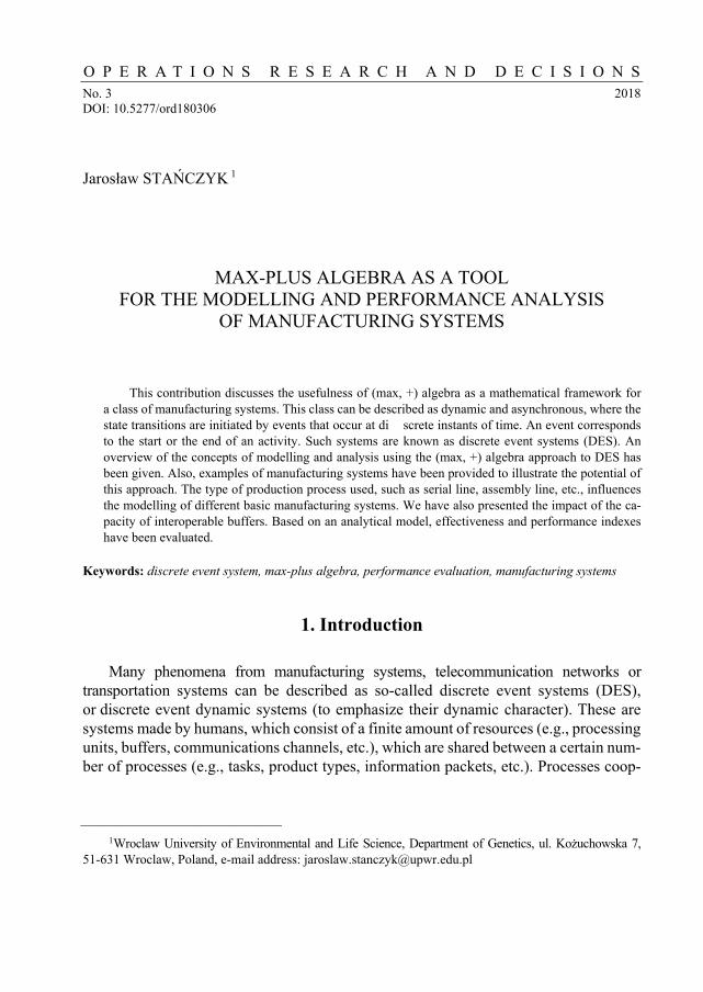
We will consider an assembly line for producing back flushing control valves [4]. Each valve consists of parts shown in Fig. 1.

Fig. 1. Valve components (from [4])

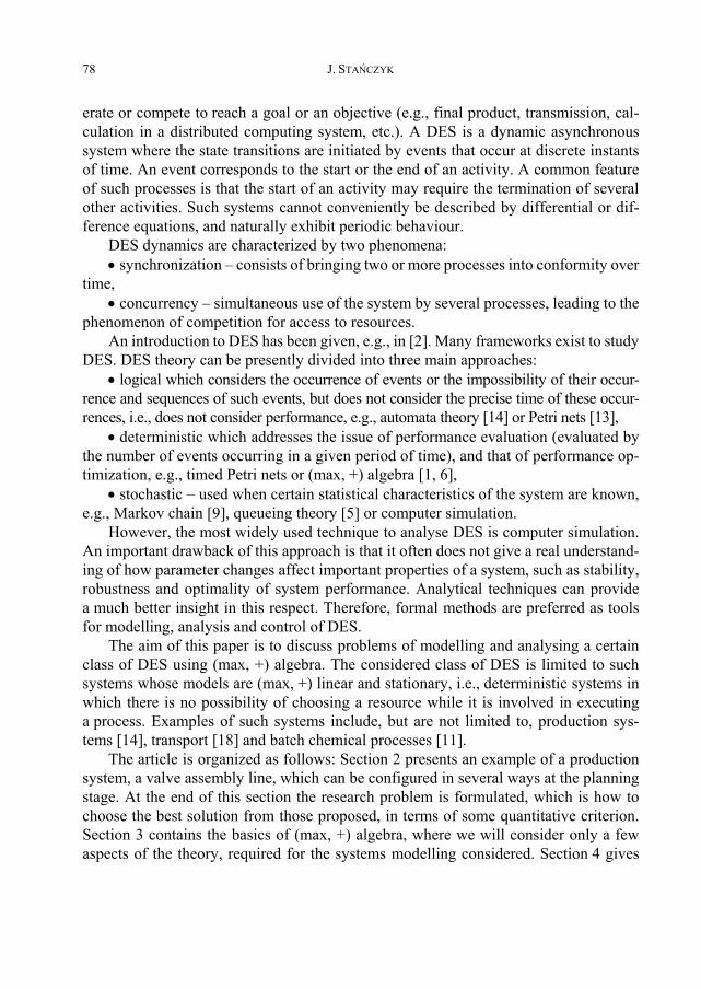
The sequence tree is shown in Fig. 2. In this tree, each node represents an independ-ent assembly operation, e.g., in the highlighted part: assembly of part number 3 with part number 4, and next with 5.

Fig. 2. Assembly sequence tree (after [7])

Translation of the sequence defined by the sequence tree into possible configura-tions of the actual production line depends on many factors, such as available space,

J. STAŃCZYK 80

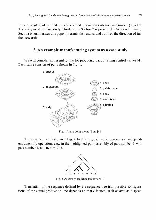
available staffing, the tools required to perform a given operation, etc. It is accomplished through appropriate production planning techniques. Assume that, at the production planning stage, 3 potential configurations of the assembly line have been obtained. All of them consist of a different number of production units. These configurations are shown in Fig. 3.

Fig. 3. Three possible assembly line configurations for the sequence tree of Fig. 2

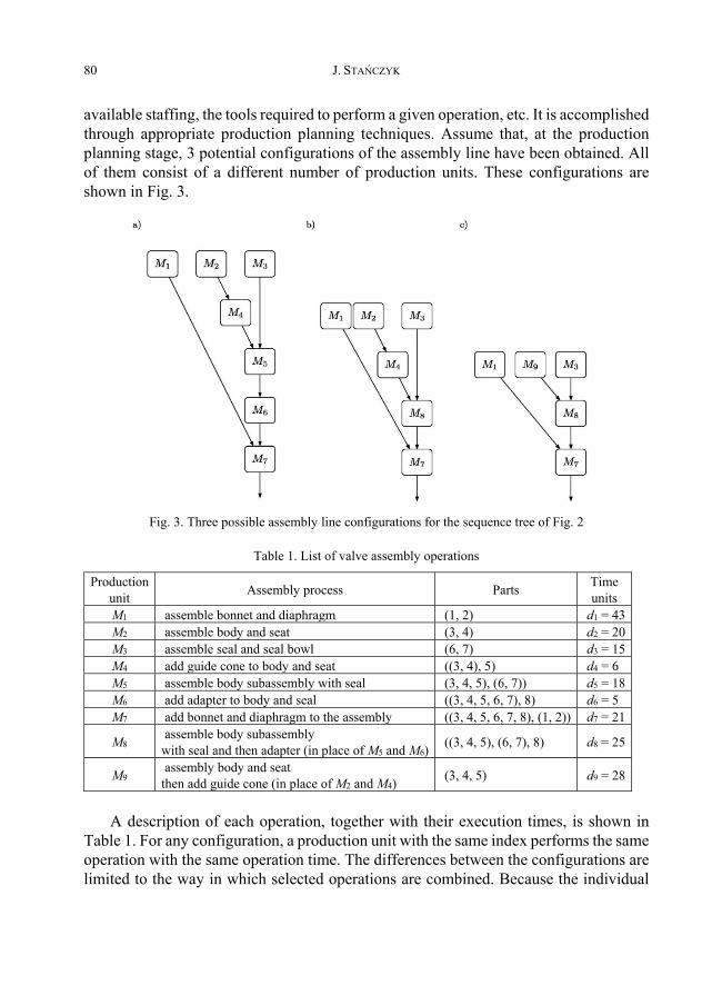
Table 1. List of valve assembly operations

Production unit Assembly process Parts Time

units M1 assemble bonnet and diaphragm (1, 2) d1 = 43 M2 assemble body and seat (3, 4) d2 = 20 M3 assemble seal and seal bowl (6, 7) d3 = 15 M4 add guide cone to body and seat ((3, 4), 5) d4 = 6 M5 assemble body subassembly with seal (3, 4, 5), (6, 7)) d5 = 18 M6 add adapter to body and seal ((3, 4, 5, 6, 7), 8) d6 = 5 M7 add bonnet and diaphragm to the assembly ((3, 4, 5, 6, 7, 8), (1, 2)) d7 = 21

M8 assemble body subassembly with seal and then adapter (in place of M5 and M6) ((3, 4, 5), (6, 7), 8) d8 = 25

M9 assembly body and seat then add guide cone (in place of M2 and M4) (3, 4, 5) d9 = 28

A description of each operation, together with their execution times, is shown in

Table 1. For any configuration, a production unit with the same index performs the same operation with the same operation time. The differences between the configurations are limited to the way in which selected operations are combined. Because the individual


configurations are similar, the problem is reduced to choosing the optimal configuration in the sense of the accepted criterion. Considering the set of given configurations, as shown in Fig. 3, the problem is formulated as follows: from the possible configurations of the assembly line choose the optimal configuration in the sense of the given criterion. For the analysis of the problem, the fastest execution time for an order consisting of N pieces was chosen as an example criterion. The solution based on the shortest down- -time is also presented. Of course, you can employ other criteria and many restrictions may be defined, such as, e.g., the capacity of interoperable buffers – as will be shown later in this paper.

3. Max-plus algebra

The (max, +) algebra was first introduced in [3]. A standard reference is [1], a brief survey of the methods and applications of this algebra is given in [6] and [8]. In certain aspects, the (max, +) algebra is comparable to conventional algebra. In the (max, +) algebra the addition (+) and multiplication (×) operators from conventional algebra are replaced by the maximization (max) and addition (+) operators, respectively. Using these operators, a linear description (in the (max, +) algebra sense) of certain non-linear systems (in conventional algebra) is achieved. In recent years, the theory of (max, +) algebra and its applications has been constantly developing and it suffices to mention a few directions: optimal control [10] predictive control [16], production modelling and planning [15, 12].

3.1. The basics

The (max, +) algebra is defined as follows:

{ }R R , where R is the field of real numbers and def= ,

, : max( , ),a b R a b a b , : .a b R a b a b

The algebraic structure def

max ( , , , , ), 0,R R e e is called the max-plus alge-bra. In this paper, the notation presented in [1] is used. This means ε and e are used instead of −∞ and 0, respectively (to emphasize their special meaning and to avoid con-fusion with their roles in conventional algebra). Additionally, the notation ab is used instead of a b everywhere where it does not cause ambiguity.

Now, we extend the (max, +) algebra operations to matrices in the following way. The sum of matrices A, B m nR

is defined to be the matrix (AB) m nR ob-

tained by adding corresponding entries. That is,

J. STAŃCZYK 82

(AB)ij = (A)ij, (B)ij, i = 1, ..., m, j = 1, ..., n (1)

The product of matrices m pRA and p nR

B is defined to be the m×n ma-trix whose (i, j)-entry is the inner product of the ith row of A with the jth column in B. That is,

1

( )p

ij k A B ((A)ik (B)ik) max

k ((A)ik (B)ik), i = 1, ..., m, j = 1, ..., n (2)

where: 1

m

jja

is short-hand for 1 ... .ma a

The matrix Inn nR with e’s on the main diagonal and ε’s else-where is called the

identity matrix of order n. The matrix n nR with εi,j = ε for all i, j is the zero matrix.

The operator * is defined for square matrix n nRA by:

0

* k

k NA A (3)

where: Ak = AAk – 1, A0 = I, 0N is the set of nonnegative integers. (3) is only mean-ingful if the right-hand side converges [3]. The operator * will be needed later, because it can be used to solve the following implicit equation for x:

x = Ax b (4)

so

x = A*b (5)

The proof can be found, e.g., in [1].

3.2. Description of the state space

One of the best-known equations defining a dynamic system is

( ) ( 1), 1, 2, ...t t t x Ax (6)

where the vector x nR is the state of the system considered, and the matrix A n nR is the state (or system) matrix. If the starting conditions are known, i.e., 0(0) ,x x then


the behaviour of the system is determined. When x nR , A ,n nR Eq. (6) written in

(max, +) algebra is as follows:

: ( ) ( 1)k N k k x A x (7)

In Equation (7) k is used instead of t, since k is not the time of an event, but the index of the cycle in which an event takes place. The most general state-space represen-tation of a (max, +)-linear system is given by:

: ( ) ( 1) ( )k N k k k x Ax Bu (8)

( ) ( ) ( )k k k y Cx Du (9)

where ,rRu ,n rRB ,mRy ,m nR

C and .m rRD

In a general case, for an Nth order system, i.e., where the N previous iterations affect the current behaviour of the system given by an implicit formula for x(k), the model is represented by:

1

00: ( ) ( ) ( )

NNi iii

k N k k i k i

x A x B u (10)

1

0( ) ( ) ( )

Ni i

ik k i k i

y C x D u (11)

After removing x(k) from the right hand side of Eq. (10) (assuming that *0A is con-

vergent) and after introducing the new vectors

( ) ( 1) ... ( 1) ,Tk k k N x x x x ( ) ( 1) ... ( 1) Tk k k N u u u u

and matrices:

* * ** *0 1 0 2 00 0 0 1

... ...

... ...,...

......

NN

A A A A A A A B A BI

A BI

0 1 0 1... , ...N N C C C D D D

J. STAŃCZYK 84

where I and ε are the (max, +)-algebraic identity and zero matrix of the appropriate sizes, a 1st order model, described by (8) and (9), is obtained.

In the rest of the paper, the part Du(k) in (9) is omitted and the equation describing takes the form:

( ) ( )k ky Cx (12)

4. Modelling manufacturing systems

Before we go back to the production system described in Section 2, let us look at modelling the individual fragments of such a system. These fragments will be then com-bined into an entire production system. Modelling simple fragments is needed to gain intuition and experience for modelling more comprehensive systems.

We start by modelling a sequential production line, i.e., a line in which individual production sites are connected in series. Then we move on to modelling an assembly line in which flow can come from several lines. Finally, we will look at the modelling of interoperability buffers.

4.1. Modelling of serial flow

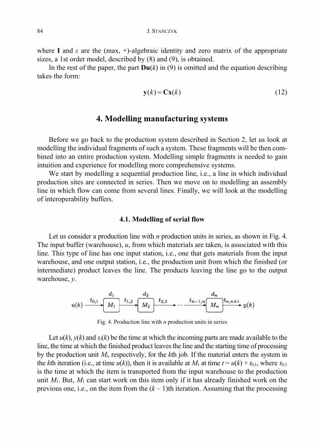
Let us consider a production line with n production units in series, as shown in Fig. 4. The input buffer (warehouse), u, from which materials are taken, is associated with this line. This type of line has one input station, i.e., one that gets materials from the input warehouse, and one output station, i.e., the production unit from which the finished (or intermediate) product leaves the line. The products leaving the line go to the output warehouse, y.

Fig. 4. Production line with n production units in series

Let u(k), y(k) and xi(k) be the time at which the incoming parts are made available to the line, the time at which the finished product leaves the line and the starting time of processing by the production unit Mi, respectively, for the kth job. If the material enters the system in the kth iteration (i.e., at time u(k)), then it is available at M1 at time t = u(k) + t0,1, where t0,1 is the time at which the item is transported from the input warehouse to the production unit M1. But, M1 can start work on this item only if it has already finished work on the previous one, i.e., on the item from the (k – 1)th iteration. Assuming that the processing


time at M1 is d1, then the item from the (k – 1)th iteration will leave the production unit at time t = x1(k − 1) + d1. We assume that this item will leave the production unit imme-diately after processing is finished and processing of the next item will start as soon as the production unit is available.

The above conditions can be translated into the following equation describing the time at which the kth item will begin to be processed on M1:

1 1 1 0,1: ( ) max ( 1), ( )k N x k d x k t u k (13)

which in (max, +) algebra is as follows:

1 1 1 0,1: ( ) ( 1) ( )k N x k d x k t u k (14)

Similarly, for production unit Mi, the kth item will start being processed by this unit when:

processing on Mi−1 has finished and it is delivered to Mi (the transportation time is ti−1,i),

processing of the (k – 1)th item on Mi has been completed. In the (max, +) algebra this is expressed as follows:

1, 1 1: ( ) ( ) ( 1)i i i i i i ik N x k t d x k d x k (15)

By combining the above equations into matrix notation:

0 1 0: ( ) ( ) ( 1) ( )k N k k k k x A x A x B u (16)

where:

1

1,2 120

1, 1

...( )

...( )( ) ,

( ) n n nn

x kt dx k

k

t dx k

x A

1 0,1

1 0

...

, , ( ) ( )

...

n

n

d td

k u k

d

A B u

J. STAŃCZYK 86

By applying the * operator, Eq. (16) can be described as Eq. (8), where: *0 1A A A

and *0 0.B A B The output of the production line is described by Eq. (12), in which:

, 1( ) ( ) and ... n n nk y k t d y C

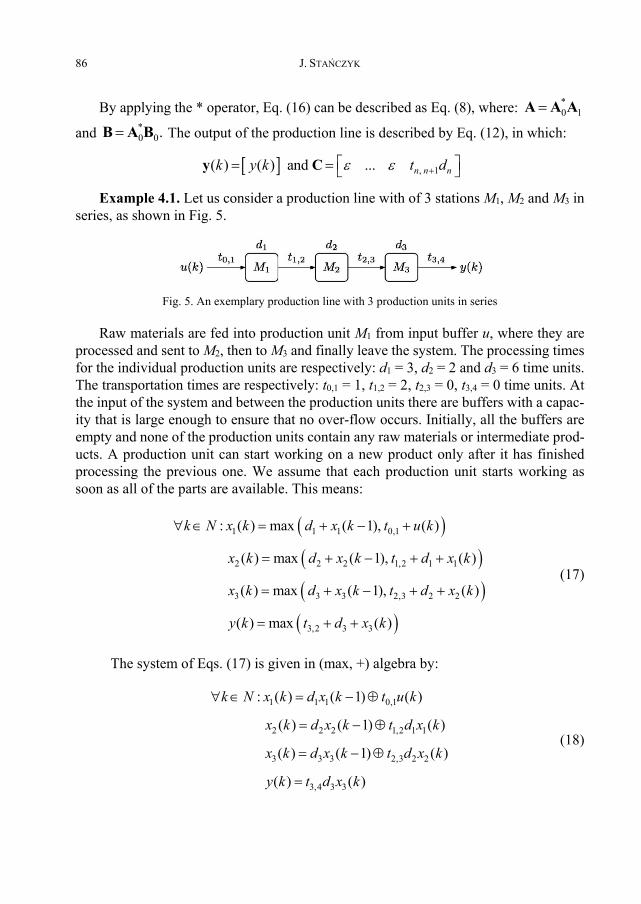
Example 4.1. Let us consider a production line with of 3 stations M1, M2 and M3 in series, as shown in Fig. 5.

Fig. 5. An exemplary production line with 3 production units in series

Raw materials are fed into production unit M1 from input buffer u, where they are processed and sent to M2, then to M3 and finally leave the system. The processing times for the individual production units are respectively: d1 = 3, d2 = 2 and d3 = 6 time units. The transportation times are respectively: t0,1 = 1, t1,2 = 2, t2,3 = 0, t3,4 = 0 time units. At the input of the system and between the production units there are buffers with a capac-ity that is large enough to ensure that no over-flow occurs. Initially, all the buffers are empty and none of the production units contain any raw materials or intermediate prod-ucts. A production unit can start working on a new product only after it has finished processing the previous one. We assume that each production unit starts working as soon as all of the parts are available. This means:

1 1 1 0,1

2 2 2 1,2 1 1

3 3 3 2,3 2 2

3,2 3 3

: ( ) max ( 1), ( )

( ) max ( 1), ( )

( ) max ( 1), ( )

( ) max ( )

k N x k d x k t u k

x k d x k t d x k

x k d x k t d x k

y k t d x k

(17)

The system of Eqs. (17) is given in (max, +) algebra by:

1 1 1 0,1

2 2 2 1,2 1 1

3 3 3 2,3 2 2

3,4 3 3

: ( ) ( 1) ( )

( ) ( 1) ( )

( ) ( 1) ( )

( ) ( )

k N x k d x k t u k

x k d x k t d x k

x k d x k t d x k

y k t d x k

(18)


Using matrix notation, this system can be written in the form of (16), then of (8), and the output equation is in the form of (12), where:

1 1

2 0 1,2 1 1 2

3 2,3 2 3

( )( ) ( ) , ,

( )

x k dk x k t d d

x k t d d

x A A

1 0,1 0,12

1,2 1 2 0 0,1 1,2 12 2

0,1 1,2 1 2,3 21,2 1 2,3 2 2,3 2 3

, ,d t t

t d d t t dt t d t dt d t d t d d

A B B

3,4 3( ) ( ) , ( ) ( ) ,k u k k y k t d u y C

After substituting in the appropriate numerical values, we obtain:

*0 1 0

3 05 , 2 , 5 0

2 6 7 2 0

A A A

0

3 1 18 2 , , 6 , 6

10 4 6 8

A B B C

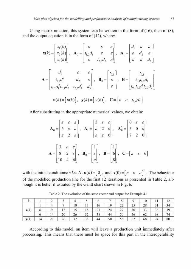
with the initial conditions: : ( ) 0 ,k N k u and (0) .T x The behaviour of the modelled production line for the first 12 iterations is presented in Table 2, alt-hough it is better illustrated by the Gantt chart shown in Fig. 6.

Table 2. The evolution of the state vector and output for Example 4.1

k 1 2 3 4 5 6 7 8 9 10 11 12

x(k) 1 4 7 10 13 16 19 22 25 28 31 34 6 9 12 15 18 21 24 27 30 33 36 39 6 14 20 26 32 38 44 50 56 62 68 74

y(k) 14 20 26 32 38 44 50 56 62 68 74 80 According to this model, an item will leave a production unit immediately after

processing. This means that there must be space for this part in the interoperability

J. STAŃCZYK 88

buffer. As shown in Fig. 6, the number of items stored in the buffer between M2 and M3 increases with each iteration. The interoperability of buffer capacity is the subject of Section 4.3.

Fig. 6. The Gantt chart for Example 4.1

4.2. Modelling the merging of lines

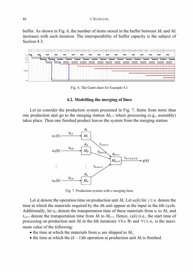
Let us consider the production system presented in Fig. 7. Items from more than one production unit go to the merging station Mn+1 where processing (e.g., assembly) takes place. Then one finished product leaves the system from the merging station.

Fig. 7. Production system with n merging lines

Let di denote the operation time on production unit Mi. Let ui(k) for i n denote the time at which the materials required by the ith unit appear at the input in the kth cycle. Additionally, let t0,i denote the transportation time of these materials from ui to Mi, and ti,n+1 denote the transportation time from Mi to Mn+1. Hence, xi(k) (i.e., the start time of processing on production unit Mi in the kth iteration) k ℕ: and ,i n is the maxi-mum value of the following:

the time at which the materials from ui are shipped to Mi, the time at which the (k – 1)th operation at production unit Mi is finished.


Analogously, xn+1(k) is the maximum of the following: the time at which the kth operation at Mi is both finished and the item transported

to Mn+1, (i = 1, 2, ..., n), the (k – 1)th operation at Mn+1 is finished. Thus, an equation of the form (16) has been obtained, where:

11

20 1

11, 1 1 , 1 1

... ...( )

( ) , ,... : . :

( )... ...n

n n n n n

dx k

dk

x kt d t d d

x A A

0,1

10,2

0

0,

...( )

, ( )( )

...nn

tu kt

ku kt

B u

The finished product reaches the output warehouse y(k) when the kth operation at production unit Mn+1 is finished and this item is transported to the warehouse, so the equation of output is expressed as in (12), in which:

( ) ( )k y ky

and

1, 2 1... n n nt d C

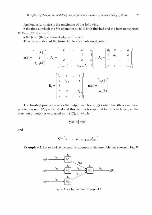
Example 4.2. Let us look at the specific example of the assembly line shown in Fig. 8.

Fig. 8. Assembly line from Example 4.2

J. STAŃCZYK 90

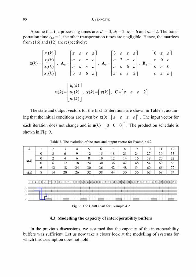
Assume that the processing times are: d1 = 3, d2 = 2, d3 = 6 and d4 = 2. The trans-portation time t2,4 = 1, the other transportation times are negligible. Hence, the matrices from (16) and (12) are respectively:

1

20 0 0

3

4

( ) 3 0( ) 2 0

( ) , , ,( ) 6 0( ) 3 3 6 2

x kx k

kx kx k

x A A B

1

2

3

( )( ) ( ) , ( ) ( ) , 2

( )

u kk u k k y k

u k

u y C

The state and output vectors for the first 12 iterations are shown in Table 3, assum-ing that the initial conditions are given by (0) .T x The input vector for

each iteration does not change and is ( ) 0 0 0 .Tk u The production schedule is shown in Fig. 9.

Table 3. The evolution of the state and output vector for Example 4.2

k 1 2 3 4 5 6 7 8 9 10 11 12

x(k)

0 3 6 9 12 15 18 21 24 27 30 33 0 2 4 6 8 10 12 14 16 18 20 22 0 6 12 18 24 30 36 42 48 54 60 66 6 12 18 24 30 36 42 48 54 60 66 72

y(k) 8 14 20 26 32 38 44 50 56 62 68 74


4.3. Modelling the capacity of interoperability buffers

In the previous discussions, we assumed that the capacity of the interoperability buffers was sufficient. Let us now take a closer look at the modelling of systems for which this assumption does not hold.


4.3.1. No buffers at all

Assume that there are no buffers between any production units. This means that an item from Mi goes to the next production unit, Mi+1, only if it is free, or the item must wait for Mi until such a time that Mi+1 would be ready to operate. To illustrate this situ-ation, consider again the system illustrated in Fig. 4. The raw materials entering the system in the kth iteration are available at M1 at time t = u(k) + t0,1. M1 can start processing the ma-terials when the previous operation is finished, i.e., at time t = x1(k − 1) + d1. In addition, production unit M1 must be ready to load the materials for the kth iteration. This means that the (k – 1)th item has already left the production unit and processing on M2 has started. Hence:

1 1 1 2 0,1: ( ) ( 1) 0 ( 1) ( )k N x k d x k x k t u k (19)

The remaining equations describing the system are formulated in the same way. If the transport time of an item from Mi to Mi+1 is significant and denoted ti,i+1, then pro-cessing at Mi should be completed before processing at Mi+1 is started, more specifically at time = −ti,i+1xi+1 instead of 0xi+1 for the case where the transportation time is insignif-icant. So, x1(k) is given by:

1 1 1 1,2 2 0,1: ( ) ( 1) ( 1) ( )k N x k d x k t x k t u k (20)

In the matrix description given by (16), the only difference occurs in the matrix A1. When there are no buffers

1 1,2

2 2,3

1

n

d td t

d

A

.

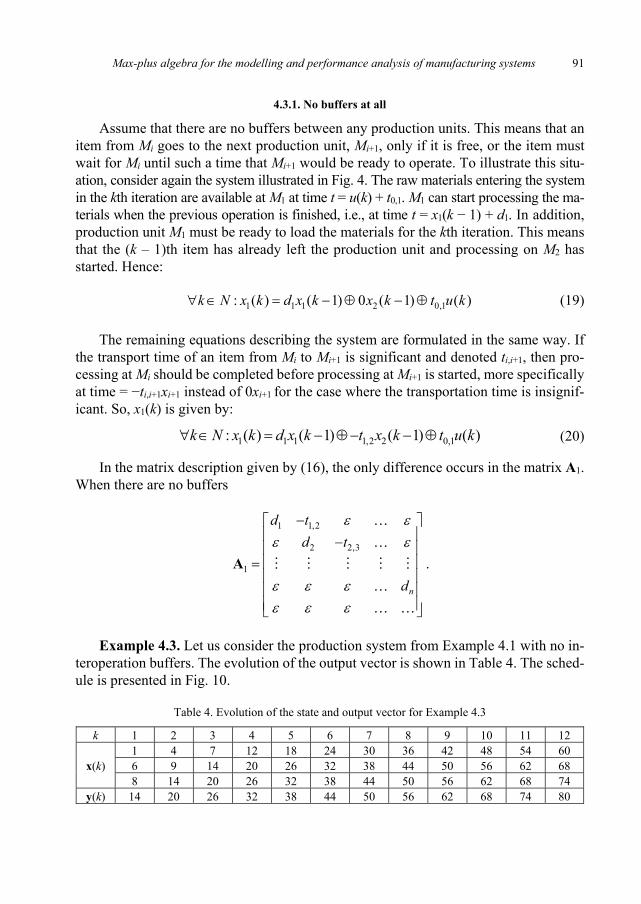
Example 4.3. Let us consider the production system from Example 4.1 with no in-teroperation buffers. The evolution of the output vector is shown in Table 4. The sched-ule is presented in Fig. 10.

Table 4. Evolution of the state and output vector for Example 4.3

k 1 2 3 4 5 6 7 8 9 10 11 12

x(k) 1 4 7 12 18 24 30 36 42 48 54 60 6 9 14 20 26 32 38 44 50 56 62 68 8 14 20 26 32 38 44 50 56 62 68 74

y(k) 14 20 26 32 38 44 50 56 62 68 74 80

J. STAŃCZYK 92


4.3.2. Buffers with a finite capacity

The modelling of finite buffers is an extension of the no buffers case. This means that if there is a buffer of capacity n between Mi and Mi+1, then (An+1)i,i+1 = 0 (if the transportation time ti,i+1 is significant, then (An+1)i,i+1 = −ti,i+1). The modelled system is described by the equation:

0 1 0: ( ) ( ) ( 1) ... ( )k N k k k k x A x A x B u (21)

This approach, as can be seen, increases the number of matrices in the model, and transformation into a model described by (16) significantly increases the size of the matrices.

Example 4.4. Let us consider the behaviour of the production system from Example 4.1 with finite buffers:

between M1 and M2 there is a buffer with capacity 1, between M2 and M3 there is a buffer with capacity 2. The model of such a system is described by the equations:

0 1 2 3 0

0

: ( ) ( ) ( 1) ( 2) ( 3) ( )

( ) ( )

k N k k k k k k

k k

x A x A x A x A x B u

y C x (22)

where

1 1 1,2

2 0 1,2 1 1 2 2

3 2,3 2 3

( )( ) ( ) , , ,

( )

x k d tk x k t d d

x k t d d

x A A A

0,1

3 0 0 3,4 30 , , ( ) ( ) , ( ) ( ) ,t

k u k k y k t d

A B u y C


After introducing a new state vector x , Eqs. (22) can be reduced to (16), and the output Eq. (12), where

1 2 3 4 5 6 7 8 9( ) ( ) ( ) ( ) ( ) ( ) ( ) ( ) ( ) ( ) Tk x k x k x k x k x k x k x k x k x kx

* * * *0 1 0 2 0 3 0 0

0, ,

A A A A A A A BA I B C C

I

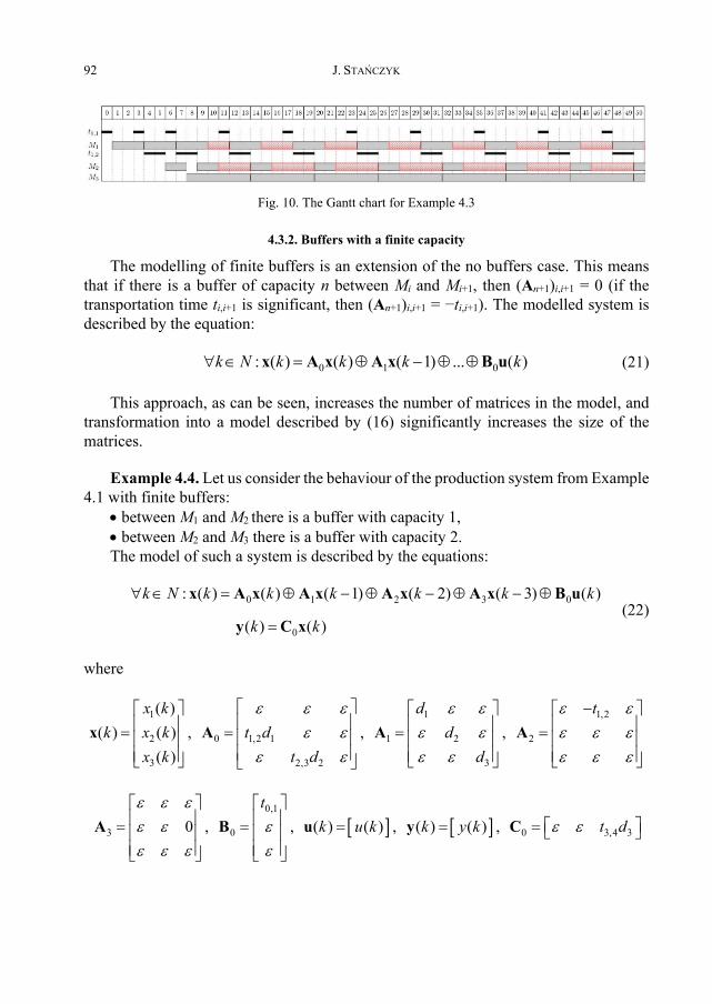
The behaviour of the modelled system, i.e., the behaviour of the first three state variables xi(k) and output y(k) is shown in Table 5 and Fig. 11.

Table 5. Evolution of the state and output vector for Example 4.4

k 1 2 3 4 5 6 7 8 9 10 11 12

x(k) 1 4 7 10 13 16 19 22 25 28 31 34 6 9 12 15 18 21 26 32 38 44 50 56 8 14 20 26 32 38 44 50 56 62 68 74

y(k) 14 20 26 32 38 44 50 56 62 68 74 80


The capacity of the interoperability buffers can also be modelled differently. A buffer of capacity n can be treated as n machines with 0 operation time and no buffers in between them. The matrices describing models generated in this way are usually smaller than those derived using the previous approach. This case is illustrated by Ex-ample 4.5.

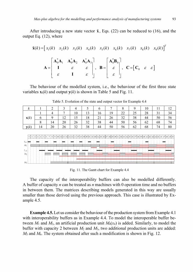
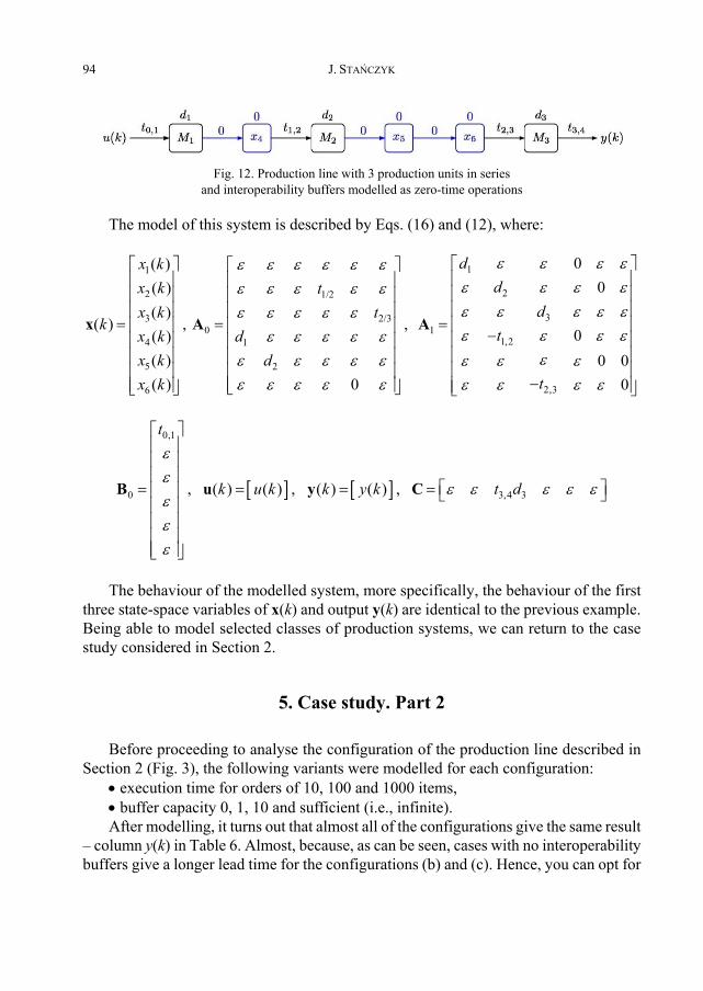
Example 4.5. Let us consider the behaviour of the production system from Example 4.1 with interoperability buffers as in Example 4.4. To model the interoperable buffer be-tween M1 and M2, an artificial production unit M4(x4) is added. Similarly, to model the buffer with capacity 2 between M2 and M3, two additional production units are added: M5 and M6. The system obtained after such a modification is shown in Fig. 12.

J. STAŃCZYK 94

Fig. 12. Production line with 3 production units in series

and interoperability buffers modelled as zero-time operations

The model of this system is described by Eqs. (16) and (12), where:

11

22 1/2

33 2/30 1

1,24 1

5 2

2,36

0( )0( )

( )( ) , ,

0( )( ) 0 0( ) 0 0

dx kdx k t

dx k tk

tx k dx k d

tx k

x A A

0,1

0 3,4 3, ( ) ( ) , ( ) ( ) ,

t

k u k k y k t d

B u y C

The behaviour of the modelled system, more specifically, the behaviour of the first three state-space variables of x(k) and output y(k) are identical to the previous example. Being able to model selected classes of production systems, we can return to the case study considered in Section 2.

5. Case study. Part 2

Before proceeding to analyse the configuration of the production line described in Section 2 (Fig. 3), the following variants were modelled for each configuration:

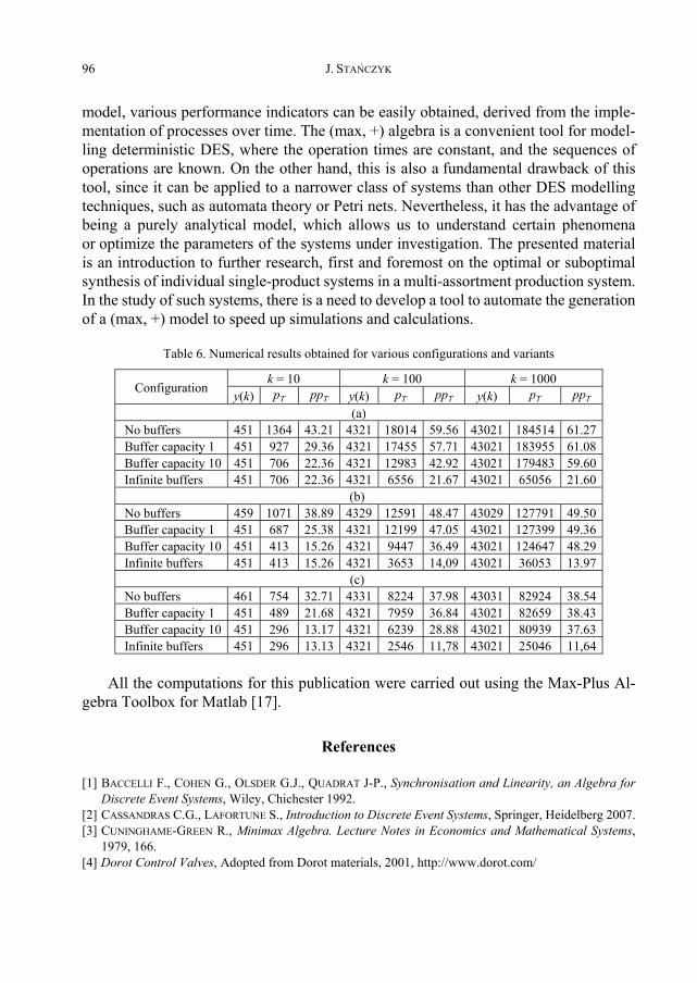
execution time for orders of 10, 100 and 1000 items, buffer capacity 0, 1, 10 and sufficient (i.e., infinite). After modelling, it turns out that almost all of the configurations give the same result

– column y(k) in Table 6. Almost, because, as can be seen, cases with no interoperability buffers give a longer lead time for the configurations (b) and (c). Hence, you can opt for


any configuration and any variant (except for the two variants mentioned above) or de-fine an additional criterion for selection. To choose one of the configurations, let us adopt minimisation of the total downtime of production units as an additional criterion. Let the downtime pi of production unit Mi in the course of m cycles be expressed by:

1

( ( ) ( ( 1) ))m

i i i ik

p x k x k d

(23)

where ( )ix k – start time of the kth operation on production unit Mi, di – processing time on Mi. It is assumed that ( ( 1) )) 0i ix k d for 1.k

The total downtime, pT, is defined as the sum of the downtimes for the individual production units (n – number of production units), i.e.,

1

n

T ii

p p

(24)

The average downtime is given by:

TT

ppn

(25)

A convenient indicator is the percentage downtime, defined as:

100%( )

TT

pppy m

(26)

where y(m) is the time at which the order is completed (output time of the mth item). After adding this new selection criterion, configuration (c) is preferred. This is because the order will be executed in the same time as for the other configurations, but in this configuration, the individual production units are released the fastest. In addition, in-creasing the capacity of the interoperability buffers further improves this index.

6. Conclusions

We encounter many complex analytical problems when designing, analysing and planning production systems. This paper presents an application of (max, +) algebra to the modelling of manufacturing systems to obtain an analytical model. Based on this

J. STAŃCZYK 96

model, various performance indicators can be easily obtained, derived from the imple-mentation of processes over time. The (max, +) algebra is a convenient tool for model-ling deterministic DES, where the operation times are constant, and the sequences of operations are known. On the other hand, this is also a fundamental drawback of this tool, since it can be applied to a narrower class of systems than other DES modelling techniques, such as automata theory or Petri nets. Nevertheless, it has the advantage of being a purely analytical model, which allows us to understand certain phenomena or optimize the parameters of the systems under investigation. The presented material is an introduction to further research, first and foremost on the optimal or suboptimal synthesis of individual single-product systems in a multi-assortment production system. In the study of such systems, there is a need to develop a tool to automate the generation of a (max, +) model to speed up simulations and calculations.

Table 6. Numerical results obtained for various configurations and variants

Configuration k = 10 k = 100 k = 1000

y(k) pT ppT y(k) pT ppT y(k) pT ppT (a)

No buffers 451 1364 43.21 4321 18014 59.56 43021 184514 61.27 Buffer capacity 1 451 927 29.36 4321 17455 57.71 43021 183955 61.08 Buffer capacity 10 451 706 22.36 4321 12983 42.92 43021 179483 59.60 Infinite buffers 451 706 22.36 4321 6556 21.67 43021 65056 21.60

(b) No buffers 459 1071 38.89 4329 12591 48.47 43029 127791 49.50 Buffer capacity 1 451 687 25.38 4321 12199 47.05 43021 127399 49.36 Buffer capacity 10 451 413 15.26 4321 9447 36.49 43021 124647 48.29 Infinite buffers 451 413 15.26 4321 3653 14,09 43021 36053 13.97

(c) No buffers 461 754 32.71 4331 8224 37.98 43031 82924 38.54 Buffer capacity 1 451 489 21.68 4321 7959 36.84 43021 82659 38.43 Buffer capacity 10 451 296 13.17 4321 6239 28.88 43021 80939 37.63 Infinite buffers 451 296 13.13 4321 2546 11,78 43021 25046 11,64

All the computations for this publication were carried out using the Max-Plus Al-

gebra Toolbox for Matlab [17].

References

[1] BACCELLI F., COHEN G., OLSDER G.J., QUADRAT J-P., Synchronisation and Linearity, an Algebra for Discrete Event Systems, Wiley, Chichester 1992.

[2] CASSANDRAS C.G., LAFORTUNE S., Introduction to Discrete Event Systems, Springer, Heidelberg 2007. [3] CUNINGHAME-GREEN R., Minimax Algebra. Lecture Notes in Economics and Mathematical Systems,

1979, 166. [4] Dorot Control Valves, Adopted from Dorot materials, 2001, http://www.dorot.com/


[5] GROSS D., SHORTIE J.F., THOMPSON J.M., HARRIS C.M., Fundamentals of Queueing Theory, Wiley, Hoboken 2008.

[6] HEIDERGOTT B., OLSDER G.J., VAN DER WOUDE J., Max Plus at Work. Modelling and Analysis of Syn-chronized Systems, Princeton University Press, Princeton 2006.

[7] KASHKOUSH M., ELMARAGHY H., Consensus tree method for generating master assembly sequence, Prod. Eng., 2014, 8, 233–242.

[8] KOMEDA J., LAHAYE S., BOIMOND J.-L., VAN DEN BOOM T., Max-plus algebra and discrete event sys-tems, IFAC Papers Online, 2017, 50 (1), 1784–1790.

[9] LIMNIOS N., OPROŞAN G., Semi-Markov Processes and Reliability, Springer Science, Business Media, New York 2013.

[10] MAIA C.A., HARDOUIN L., SANTOS-MENDES R., COTTENCEAU B., Optimal closed-loop control of timed event graphs in dioids, IEEE Trans. on Automatic Control, 2003, 12, 2284–2287.

[11] MUTSAERS M., ÖZKAN L., BACKX T., Scheduling of energy flows for parallel batch processing using max-plus systems, Proc. 8 IFAC Symposium on Advanced Control of Chemical Processes, Singapore, 2012.

[12] NAMBIAR A.N., IMAEV A., JUDD R.P., CARLO H.J., Production planning models using max-plus alge-bra, [In:] V. Modrak, R.S. Pandian (Eds.), Operations management research and cellular manufac-turing systems, IGI Global, Hershey 2012, 227–257.

[13] PETRI C.A., Kommunikation mit Automaten, PhD Thesis, University of Bonn, 1962. [14] RAMADGE P.J., WONHAM W.M., The control of discrete event systems, Proc. of the IEEE, 1989, 77,

81–98. [15] SELEIM A., EL MARAGHY H., Max-plus modeling of manufacturing flow lines, Proc. 47 CIRP Confer-

ence Manufacturing Systems (CMS2014), 2014, 17, 302–307. [16] SEYBOLD L., WITCZAK M., MAJDZIK P., STETTER R., Towards robust predictive fault-tolerant control

for a battery assembly system, Int. J. Appl. Math. Comp. Sci., 2015, 25 (4), 849–862. [17] STAŃCZYK J., Max-Plus Algebra Toolbox for Matlab ver. 1.7, 2016, http://gen.up.wroc.pl/stanczyk/mpa/ [18] STAŃCZYK J., MAYER E., RAISCH J., Modelling and performance evaluation of DES, Proc. International

Conference Informatics in Control, Automation and Robotics, Setubal, Portugal, 2004, 3, 270–275.

Received 9 October 2017 Accepted 14 August 2018

Date post:	05-Nov-2021
Category:	Documents
Upload:	others
View:	2 times
Download:	0 times

MAX-PLUS ALGEBRA AS A TOOL FOR THE MODELLING AND ...

Documents