105
Maximizing Fuel Economy of Power Split Hybrid Electric Vehicle ME 555 Term Project Shubham Khadria: 13382389 Shounak Bapat: 31341331 Pradeep Kodali: 69416665 Vijay Kumar Singla: 45228918

Maximizing Fuel Economy of Power Split
Hybrid Electric Vehicle ME 555 Term Project
Shubham Khadria: 13382389 Shounak Bapat: 31341331 Pradeep Kodali: 69416665
Vijay Kumar Singla: 45228918
Contents I) SUBSYSTEM: CAR RADIATOR ..................................................................................................................... 6
1. INTRODUCTION ..................................................................................................................................... 6
2. PROBLEM STATEMENT .......................................................................................................................... 7
OBJECTIVE ............................................................................................................................................. 7
ASSUMPTIONS ...................................................................................................................................... 8
MATHEMATICAL MODEL ....................................................................................................................... 8
NOMENCLATURE ................................................................................................................................. 10
DESIGN VARIABLE ............................................................................................................................... 12
DESIGN PARAMETERS ......................................................................................................................... 12
DESIGN CONSTRAINTS ........................................................................................................................ 14
FEASIBLE POINT ................................................................................................................................... 15
3. MATLAB RESULTS ................................................................................................................................ 15
4. RESULT AND DISCUSSIONS .............................................................................................................. 16
II) ENGINE SUBSYSTEM: Shounak Bapat ..................................................................................................... 17
1. INTRODUCTION: .................................................................................................................................. 17
VARIABLES: .......................................................................................................................................... 17
ASSUMPTIONS: ................................................................................................................................... 18
2. NOMENCLATURE: ................................................................................................................................ 19
3. DIESEL ENGINE MODEL: ...................................................................................................................... 20
AMESIM Model ................................................................................................................................... 20
OBJECTIVE FUNCTION: ........................................................................................................................ 23
CONSTRAINTS: .................................................................................................................................... 23
OVERALL MODEL: ................................................................................................................................ 23
MONOTONICITY TABLE: ...................................................................................................................... 25
4. OPTIMIZATION RESULTS: .................................................................................................................... 26
SUMMARIZED RESULT: ....................................................................................................................... 27
5. PARAMETRIC SWEEP: .......................................................................................................................... 28
CONSTRAINT RELAXATION: [RELAX LOWER BOUND] ......................................................................... 28
VARIATION IN ENGINE SPEED: ............................................................................................................ 30
VARIATION IN MASS OF FUEL INJECTED [INJECTION DURATION]: ..................................................... 32
CONCLUSION: ...................................................................................................................................... 33
1

III) ELECTRICAL SUBSYSTEM ........................................................................................................................ 34
1. INTRODUCTION ................................................................................................................................... 34
ABOUT AMESIM .................................................................................................................................. 34
COMPONENTS OF THE SUBSYSTEM .................................................................................................... 34
PROBLEM DEFINITION............................................................................................................................. 38
ASSUMPTIONS .................................................................................................................................... 38
DESIGN PARAMETERS ......................................................................................................................... 38
DESIGN VARIABLES .............................................................................................................................. 39
CONSTRAINTS ON DESIGN VARIABLES ................................................................................................ 41
OBJECTIVE FUNCTION ......................................................................................................................... 41
OPTIMIZATION PROBLEM ................................................................................................................... 42
APPROACH .............................................................................................................................................. 43
GENETIC ALGORITHM ......................................................................................................................... 43
RESULTS OF GENETIC ALGORITHM ..................................................................................................... 44
FMINCON WITH SQP ALGORITHM ...................................................................................................... 45
RESULTS OF FMINCON ........................................................................................................................ 47
FINAL RESULTS ........................................................................................................................................ 47
SENSITIVITY ANALYSIS – FOR SYSTEM OPTIMIZATION ........................................................................... 48
GENERATION OF MAPS ....................................................................................................................... 48
CONCLUSION OF ELECTRICAL SUBSYSTEM ............................................................................................. 50
ACKNOWLEDGEMENTS ....................................................................................................................... 50
IV) TRANSMISSION SUBSYSTEM .................................................................................................................. 51
1 PROBLEM STATEMENT ......................................................................................................................... 51
2 ASSUMPTIONS...................................................................................................................................... 51
3 NOMENCLATURE .................................................................................................................................. 51
4 OBJECTIVE ............................................................................................................................................ 52
5 VARIABLES ............................................................................................................................................ 52
6 PARAMETERS ....................................................................................................................................... 52
7 Constraints ........................................................................................................................................... 52
8 PLANETARY GEAR MODEL .................................................................................................................. 53
9 VARIATION OF FUEL CONSUMPTION WITH CHANGE IN VARIABLES ................................................... 55
10 MODEL OPTIMISATION ...................................................................................................................... 57
11 SUBSYSTEM OPTIMISATION ............................................................................................................... 60
2

12 RESULT DISCUSSION ........................................................................................................................... 60
V) SYSTEM OPTIMIZATION .......................................................................................................................... 61
1. PROBLEM STATEMENT ........................................................................................................................ 61
2. MATHEMATICAL MODEL ..................................................................................................................... 61
4. OPTIMIZATION RESULTS ..................................................................................................................... 63
5. SYSTEM ANALYSIS ............................................................................................................................... 63
6 CONCLUSION ........................................................................................................................................ 64
VI) REFERENCES ........................................................................................................................................... 67
VI) APPENDIX ............................................................................................................................................... 68
A) MATLAB CODE – Radiator Subsystem (SHUBHAM KHADRIA) ........................................................ 68
Code for optimization ......................................................................................................................... 68
Code for Modelling the radiator ......................................................................................................... 69
B) Engine Subsystem-BFSC MAPS and MATLAB code (SHOUNAK BAPAT) .......................................... 72
BSFC Maps: .......................................................................................................................................... 72
MATLAB Code for Subsystem Optimization:....................................................................................... 73
MATLAB Code for generating fuel consumption maps:...................................................................... 75
C) MATLAB Code – Electrical Subsystem (Pradeep Kodali) ................................................................. 78
RRR) MATLAB Code – Planetary Gear system (Vijay Kumar Singla) .................................................... 95
3
Table 1 Set of Initial values ..................................................................................................................... 15 Table 2 Design variable with their reference........................................................................................ 15 Table 3 Matlab result for different sets of inital value ......................................................................... 16 Table 4 Engine Subsystem Variables List ............................................................................................ 19 Table 5 Engine Subsystem Parameters list ......................................................................................... 19 Table 6 Engine Subsystem Monotonicity Analysis ............................................................................. 25 Table 7 Engine Subsystem Optimization Results ............................................................................... 26 Table 8 Engine Subsystem Constraint relaxation ............................................................................... 28 Table 9 Engine Subsystem Variation in RPM ...................................................................................... 30 Table 10 Engine Subsystem Injection Duration Variation .................................................................. 32 Table 11 Subsystem Optimisation results ............................................................................................ 60 Table 12 System level optimization ....................................................................................................... 63
Figure 1 Diagram of a Car Radiator ........................................................................................................ 6 Figure 2 drawing of a radiator design to highlight various variables [Ref. E Y Ng et al.] ................ 7 Figure 3 AMESIM Diesel Engine Model ............................................................................................... 22 Figure 4 BSFC v/s CR ............................................................................................................................. 24 Figure 5 BSFC v/s Bore .......................................................................................................................... 24 Figure 6 BSFC v/s stroke ........................................................................................................................ 24 Figure 7 BSFC v/s Injection Timing ....................................................................................................... 24 Figure 8 Simulink model of planetary gear subsystem ...................................................................... 54 Figure 9 Simulink model of the Power Split Hybrid vehicle with rule based control ...................... 55 Figure 10 Variation in fuel consumption corresponding to variation in Final Drive Ratio .............. 56 Figure 11 Variation in fuel consumption corresponding to variation in No. of sun gears .............. 56 Figure 12 Variation in fuel consumption corresponding to variation in No. of ring gears.............. 57 Figure 13 Plot of f (SOC) with variation in SOC .................................................................................. 58 Figure 14 Surface plot for Engine optimal power obtained by using ECMS ................................... 59 Figure 15 ECMS control implemented in Power Management of the Simulink Model .................. 59
4

Introduction to the System In today’s world, where the limited amounts of fossil fuel resources and with the rising threat to
human health from vehicular emissions it is necessary to develop vehicles that have high
efficiency and low emissions. One such solution is the class of Hybrid electric vehicles. The HEV
consist of an internal combustion engine and a battery- motor system. The radiator cools the
engine and in some cases a dedicated battery cooling system is present to dissipate heat from
the battery. In addition to these, the planetary gear system is the most critical part as it chooses
the distribution of power amongst the engine and the battery.
This study attempts to optimize the mileage of a HEV based on optimization of the above
mentioned four subsystems. Thus, the overall objective of the system is to minimize the ‘miles
per gallon’ for the HEV such that it shows controlled deviation of velocity output from the drive
cycle. The radiator (cooling fan) effects the working of the engine. Electrical system and engine
inefficiencies (heat loss) also lead to lower vehicle efficiency. To meet the Corporate Average
Fuel Economy (CAFÉ) targets of 55mpg by 2025, there is a need of a strong and concerted effort
to push the automobile efficiency above 60mph. The hybridization of the vehicle can play a crucial
role in achieving this.
Subsystem level goal for radiator was to optimize the radiator design for a given heat dissipation
requirement and dimensional constraint and minimize the coolant temperature outlet to put a
lower bound on the wall temperature for the engine cylinder. Thus, the subsystem level
optimization goal for the engine subsystem was to minimize the brake specific fuel consumption
(BSFC). Subsystem level goal for electrical subsystem was to maximize the efficiency. Subsystem
level goal for planetary gear subsystem was to optimize the fuel economy.
1. Radiator Subsystem – Shubham Khadria
2. Engine Subsystem – Shounak Bapat
3. Electrical Subsystem – Pradeep Kodali
4. Planetary Gear subsystem – Vijay Kumar Singla
5
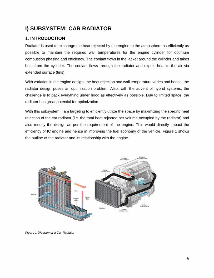
I) SUBSYSTEM: CAR RADIATOR 1. INTRODUCTION Radiator is used to exchange the heat rejected by the engine to the atmosphere as efficiently as
possible to maintain the required wall temperatures for the engine cylinder for optimum
combustion phasing and efficiency. The coolant flows in the jacket around the cylinder and takes
heat from the cylinder. The coolant flows through the radiator and expels heat to the air via
extended surface (fins).
With variation in the engine design, the heat rejection and wall temperature varies and hence, the
radiator design poses an optimization problem. Also, with the advent of hybrid systems, the
challenge is to pack everything under hood as effectively as possible. Due to limited space, the
radiator has great potential for optimization.
With this subsystem, I am targeting to efficiently utilize the space by maximizing the specific heat
rejection of the car radiator (i.e. the total heat rejected per volume occupied by the radiator) and
also modify the design as per the requirement of the engine. This would directly impact the
efficiency of IC engine and hence in improving the fuel economy of the vehicle. Figure 1 shows
the outline of the radiator and its relationship with the engine.
Figure 1 Diagram of a Car Radiator
6

Figure 2 drawing of a radiator design to highlight various variables [Ref. E Y Ng et al.]
2. PROBLEM STATEMENT OBJECTIVE
The heat dissipation would be maximum at lower engine wall temperatures which would result
from the lower temperatures of the coolant. Hence, to design a robust radiator, the problem was
framed to optimize the radiator design for a given heat dissipation requirement and dimensional
constraint and minimize the coolant temperature outlet to put a lower bound on the wall
temperature for the engine.
The objective problem was to minimize the outlet temperature of the coolant
f = min (Tc_out)
7

ASSUMPTIONS
1. The cooling system operates under steady state conditions, i.e. a constant coolant
flowrate and fluid temperatures at both inlets.
2. Heat carried by the coolant only transfers to the airflow that travels through the radiator.
Any other heat losses to, or heat gains from, the surroundings are negligible.
3. There are no phase changes in the fluid streams flowing through the radiator.
4. Longitudinal heat conduction in the fluid and in the wall is negligible.
5. The coolant flowrate in coolant tubes is uniformly distributed through the radiator, with no
flow misdistribution, flow stratification, flow bypassing, or flow leakage occurring.
6. Coolant flow is in a fully developed condition in each tube.
7. Both fluids are considered incompressible flow, and unmixed at any cross-section
between passes. The term ‘unmixed’ is defined as each fluid through the radiator that
behaves as if it was divided into a large number of separate passages with no lateral
mixing.
8. All dimensions are uniform throughout the radiator and the heat transfer surface area is
consistent and distributed uniformly.
9. There are no heat sources and sinks in the radiator walls or fluids.
10. Pure water is used as the coolant.
11. The thermal conductivity of the radiator material is constant.
12. The thermal resistance (fouling) induced by fluid impurities, rust formation, or other
reactions between the fluids and the material is assumed to be small.
MATHEMATICAL MODEL
A set of 1-D heat transfer equations based on reference [1] [2] for extended surface was modelled
using MATLAB (code shared in the appendix A). The input is the dimensions of the extended
surface, heat rejection and outputs are the dimensions of radiator core and the coolant outlet
temperature.
Effectiveness – NTU (ε- NTU) Method [2] was used to build a Mathematical Model of heat transfer
in a radiator. The basic working can be understood by following equations.
Following equations were modelled:
1. Initial Temperature Difference (ITD)
ITD = Coolant Temperature - Air Temperature
8

2. Overall Heat Transfer Coefficient:
3. Number of Transfer Units (NTU)
Cmin = Cc or Ca whichever is smaller.
4. ε- NTU Relation for a Cross-flow heat exchanger with unmixed fluids:
A mathematical expression of heat exchange effectiveness vs. the number of transfer
units:
Where,
5. Heat Transfer Equation:
The rate of conductive heat transfer
Apart from the above equations the other intermediate equations used to build the complete
model are as given below.
1. Reynolds Number:
A dimensionless modulus that represents fluid flow conditions:
2. Nusselt Number:
It gives the ratio of convective heat transfer to conductive heat transfer over a boundary. Larger
Nusselt number corresponds to greater convective heat transfer which is a characteristic of
turbulent flow.
3. Extended Surfaces
Equations to calculate the efficiency of extended surfaces were modeled.
9
4. Heat transfer coefficient for air and coolant at different Reynolds number.
5. The equation for the dimension of the radiator.
• Bh = Fh *(Nct -1) - Nct *Ycw
• Bw= Y1
• Bt = (Nr-1)-Nr *Ycl
• Ycl = Ft *Np – Lp *(Np-1)
Equations to calculate heat transfer coefficient for different fluid properties and Reynolds number
were modeled.
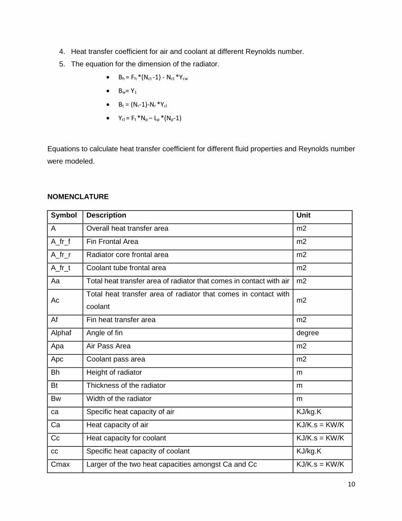
NOMENCLATURE
Symbol Description Unit
A Overall heat transfer area m2
A_fr_f Fin Frontal Area m2
A_fr_r Radiator core frontal area m2
A_fr_t Coolant tube frontal area m2
Aa Total heat transfer area of radiator that comes in contact with air m2
Ac Total heat transfer area of radiator that comes in contact with
coolant m2
Af Fin heat transfer area m2
Alphaf Angle of fin degree
Apa Air Pass Area m2
Apc Coolant pass area m2
Bh Height of radiator m
Bt Thickness of the radiator m
Bw Width of the radiator m
ca Specific heat capacity of air KJ/kg.K
Ca Heat capacity of air KJ/K.s = KW/K
Cc Heat capacity for coolant KJ/K.s = KW/K
cc Specific heat capacity of coolant KJ/kg.K
Cmax Larger of the two heat capacities amongst Ca and Cc KJ/K.s = KW/K
10
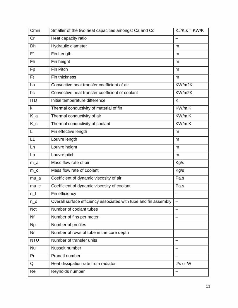
Cmin Smaller of the two heat capacities amongst Ca and Cc KJ/K.s = KW/K
Cr Heat capacity ratio –
Dh Hydraulic diameter m
F1 Fin Length m
Fh Fin height m
Fp Fin Pitch m
Ft Fin thickness m
ha Convective heat transfer coefficient of air KW/m2K
hc Convective heat transfer coefficient of coolant KW/m2K
ITD Initial temperature difference K
k Thermal conductivity of material of fin KW/m.K
K_a Thermal conductivity of air KW/m.K
K_c Thermal conductivity of coolant KW/m.K
L Fin effective length m
L1 Louvre length m
Lh Louvre height m
Lp Louvre pitch m
m_a Mass flow rate of air Kg/s
m_c Mass flow rate of coolant Kg/s
mu_a Coefficient of dynamic viscosity of air Pa.s
mu_c Coefficient of dynamic viscosity of coolant Pa.s
n_f Fin efficiency –
n_o Overall surface efficiency associated with tube and fin assembly –
Nct Number of coolant tubes –
Nf Number of fins per meter –
Np Number of profiles
Nr Number of rows of tube in the core depth
NTU Number of transfer units –
Nu Nusselt number –
Pr Prandtl number –
Q Heat dissipation rate from radiator J/s or W
Re Reynolds number –
11

Rf Fin end radius m
Rho_a Density of air kg/m3
Rho_c Density of coolant kg/m3
Rt Coolant tube end radius m
Ta_in Ambient air temperature K
Tc_in Temperature of coolant coming out of engine core K
U Overall heat transfer coefficient KW/m2K
Va Velocity of air m/s
Y1 coolant tube length (equals the width of the radiator) m
Ycl Coolant tube cross sectional length m
Ycw Coolant tube cross sectional width m
Yp Coolant tube pitch( surface distance between 2 tubes) m
Yt Coolant tube thickness m
ε Overall Effectiveness –
DESIGN VARIABLE
Based on literature review and initial sensitivity check of model for all data variables, following
were identified as the design variables for this problem. The rest were not very influential and
were taken as design parameters to reduce the modelling complexity. The focus was to provide
the best possible metamodel to approximate the functioning of real radiator.
• No. of coolant tubes in one row • No. of rows of tube in the core depth
• Coolant tube length
• Fin Height
• No. of Profiles (No of fins in the depth direction per coolant tube)
• Fin width
• Coolant tube cross section width
• Coolant Inlet temperature.
DESIGN PARAMETERS
• Heat dissipation requirement Qmin= 40KW X 2 (Taken from Engine subsystem)
12
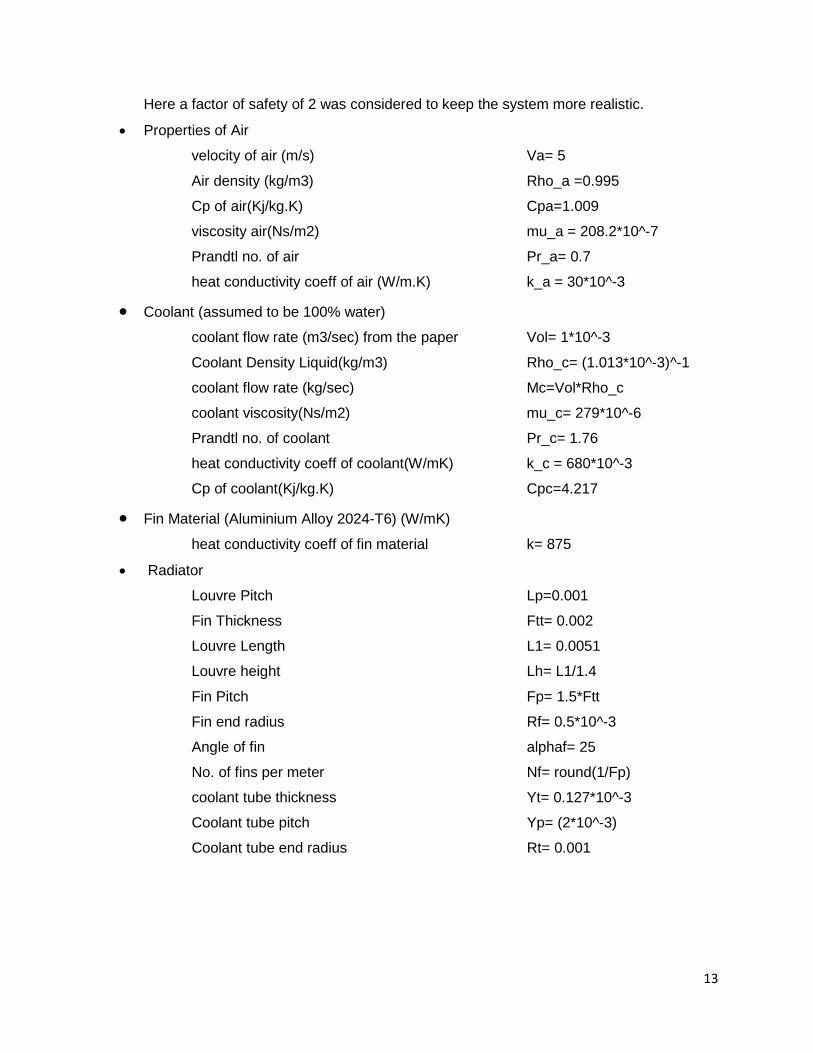
Here a factor of safety of 2 was considered to keep the system more realistic.
• Properties of Air
velocity of air (m/s) Va= 5 Air density (kg/m3) Rho_a =0.995 Cp of air(Kj/kg.K) Cpa=1.009 viscosity air(Ns/m2) mu_a = 208.2*10^-7 Prandtl no. of air Pr_a= 0.7 heat conductivity coeff of air (W/m.K) k_a = 30*10^-3
• Coolant (assumed to be 100% water) coolant flow rate (m3/sec) from the paper Vol= 1*10^-3 Coolant Density Liquid(kg/m3) Rho_c= (1.013*10^-3)^-1 coolant flow rate (kg/sec) Mc=Vol*Rho_c coolant viscosity(Ns/m2) mu_c= 279*10^-6 Prandtl no. of coolant Pr_c= 1.76 heat conductivity coeff of coolant(W/mK) k_c = 680*10^-3 Cp of coolant(Kj/kg.K) Cpc=4.217
• Fin Material (Aluminium Alloy 2024-T6) (W/mK) heat conductivity coeff of fin material k= 875
• Radiator
Louvre Pitch Lp=0.001
Fin Thickness Ftt= 0.002
Louvre Length L1= 0.0051
Louvre height Lh= L1/1.4
Fin Pitch Fp= 1.5*Ftt
Fin end radius Rf= 0.5*10^-3
Angle of fin alphaf= 25
No. of fins per meter Nf= round(1/Fp)
coolant tube thickness Yt= 0.127*10^-3
Coolant tube pitch Yp= (2*10^-3)
Coolant tube end radius Rt= 0.001
13

DESIGN CONSTRAINTS
Bounds
From literature review, a maximum limit on the dimensions of radiator were identified. An initial
15% reduction on each dimension was applied and based on that following bounds were applied
on height, width and thickness of the radiator. After an initial sensitivity test, these bounds were
later on further reduced to put additional dimensional constraints.
1. Width of the radiator
g(1)= Bw-0.30 ≤ 0
2. Height of the radiator
g(2)= Bh-0.30 ≤ 0
3. Thickness of the radiator
g(3)= Bt-0.025 ≤ 0
4. To avoid division by zero, a lower limit infinitesimally greater than 0 was set
g(11)=-Bw+0.01 ≤ 0
g(12)=-Bh+0.01 ≤ 0
g(13)=-Bt+0.01 ≤ 0
g(14)= -Apa+0.001 ≤ 0
g(15)=-Ycw+0.002 ≤ 0
g(16)= -Ycl+0.01 ≤ 0
Inequality constraints used in the model are described as follows:
5. Number of cooling tubes in one row of cooling tubes
g(4)=-Nct+2 ≤ 0
6. Number of rows of coolant tube along the thickness of the radiator
g(5)=-Nr+1 ≤ 0
7. Coolant tube length
g(6)=-Y1+0.01 ≤ 0
8. Fin height
g(7)=-Fh+0.005 ≤ 0
9. Number of profiles
g(8)=-Np+1 ≤ 0
10. Fin width
14

g(9)=-Ft+0.005 ≤ 0
11. Effectiveness of the extended surface
g(10)= -effect+2 ≤ 0
12. The Heat dissipation should be greater than the minimum requirement of the design
g(17)=(+Qmin-Q) ≤ 0
13. Lower temperature limit on the outlet temperature of the coolant
g(18)= (-Tc_in+Tc_out) ≤ 0
FEASIBLE POINT
6 set of feasible initial values were identified to test the function.
Table 1 Set of Initial values
Table 2 Design variable with their reference
Variable Reference
No. of coolant tubes in one row X(1)
No. of rows of tube in the core depth X(2)
Coolant tube length X(3)
Fin Height X(4)
No. of Profiles (No of fins in the depth direction per coolant tube) X(5)
Fin width X(6)
Coolant tube cross section width X(7)
Coolant Inlet temperature X(8)
3. MATLAB RESULTS Fmincon function was used with different initial values with two algorithm- Active set strategy and
Sequential quadratic programing to compare the result. The values converged to a similar values
with different starting points.
15

Table 3 Matlab result for different sets of inital value
Based on the output of various values, a set of variables minimizing the temperature were
identified. Since all the starting points with different models converged to the same value, we can
conclude the values are global minima.
The coolant outlet temperature (Tc_out): 428 K
4. RESULT AND DISCUSSIONS 1. Based on the output from various initial values and algorithm, a global convergence was
achieved.
2. The value of minimum outlet temperature of coolant from the heat exchanger was
achieved at 428K (155 °C).
3. Radiator was able to dissipate heat at 80 KW rate which was taken as a design parameter
from the engine subsystem.
4. No. of iterations taken by the system was around 20.
5. The dimension of the radiator converged to upper limit. This was expected as the heat
dissipation depends on the size of the radiator.
6. The average of inlet and outlet temperature (165 °C) is used in setting the lower bound for
the engine design.
16
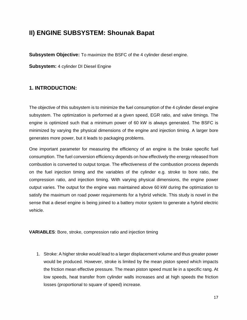
II) ENGINE SUBSYSTEM: Shounak Bapat
Subsystem Objective: To maximize the BSFC of the 4 cylinder diesel engine.
Subsystem: 4 cylinder DI Diesel Engine
1. INTRODUCTION:
The objective of this subsystem is to minimize the fuel consumption of the 4 cylinder diesel engine
subsystem. The optimization is performed at a given speed, EGR ratio, and valve timings. The
engine is optimized such that a minimum power of 60 kW is always generated. The BSFC is
minimized by varying the physical dimensions of the engine and injection timing. A larger bore
generates more power, but it leads to packaging problems.
One important parameter for measuring the efficiency of an engine is the brake specific fuel
consumption. The fuel conversion efficiency depends on how effectively the energy released from
combustion is converted to output torque. The effectiveness of the combustion process depends
on the fuel injection timing and the variables of the cylinder e.g. stroke to bore ratio, the
compression ratio, and injection timing. With varying physical dimensions, the engine power
output varies. The output for the engine was maintained above 60 kW during the optimization to
satisfy the maximum on road power requirements for a hybrid vehicle. This study is novel in the
sense that a diesel engine is being joined to a battery motor system to generate a hybrid electric
vehicle.
VARIABLES: Bore, stroke, compression ratio and injection timing
1. Stroke: A higher stroke would lead to a larger displacement volume and thus greater power
would be produced. However, stroke is limited by the mean piston speed which impacts
the friction mean effective pressure. The mean piston speed must lie in a specific rang. At
low speeds, heat transfer from cylinder walls increases and at high speeds the friction
losses (proportional to square of speed) increase.
17

2. Bore: The bore to stroke ratio is limited by engine packaging constraint and mechanical
constraints from bore to stroke ratio. A larger bore would lead to greater power.
3. Compression ratio: A higher compression ratio leads to higher engine efficiency. However,
the maximum compression ratio is limited by the maximum level of peak pressures that
can be tolerated by the engine. If pressures exceed this limit, failure of engine may occur.
4. Injection Timing: Injection timing controls the phasing of combustion in the engine. Ideally,
the injection timing should be such that the CA50 lies in the range of 6 to 10 CAD ATDC.
In the present study, the lower and upper bounds on injection timing are placed to ensure
operation in normal diesel engine regime. Late injection timings can lead to lower
combustion efficiency and too early injections would lead to higher cylinder temperatures
and there by generate higher NOx.
ASSUMPTIONS:
1. No analysis of mechanical or thermal stresses due to pressure and temperature was
considered. The cap on engine design due to stress considerations was reflected in form
of maximum limit of compression ratio.
2. Effect of valve timings is not considered. The inlet and exhaust valve overlap can affect
the amount of EGR within the cylinder. However, in the optimization, their values were not
varied.
3. A minimum power requirement of 60 kW is assumed. The minimum power requirement is
based on typical engine power requirements in hybrid vehicles.
4. Weight and mechanical stress constraints are adequately represented in the bounds on
bore size. The bounds were adopted from Heywood
5. Combustion is not resolved into premixed and diffusion burn.
18

2. NOMENCLATURE:
Variables:
Symbol Description Units
B Bore size mm
S Stroke size mm
CR Compression Ratio ---
InjTiming Injection timing CAD BTDC Table 4 Engine Subsystem Variables List
Intermediate Variables:
Symbol Description Units
P Power generated kW
Vd Sweep volume m^3
Vc Clearance Volume m^3
Vp Mean Piston speed m/s
Parameters:
Table 5 Engine Subsystem Parameters list
Symbol Description Value Units
length Connecting rod length 150 mm
squish Engine squish height 0.8 mm
Ncyl Number of cylinders 4 --
T_fuel Injected fuel temperature 293 K
P_fuel Injected fuel pressure 1000 bar
Twall Wall temperature 533 K
EGR_valve EGR gas used 7% --
RPM Engine Speed 3000 rpm
Fuel_injected Mass of fuel injected per cycle 103 mg
19

3. DIESEL ENGINE MODEL:
AMESIM Model
The engine subassembly is generated using a simulation model in AMESim software. The model
has 4 cylinders and an EGR loop which is set to achieve a 7% burned gas fraction in the intake
manifold. Fuel is injected into the cylinder directly via a single injector on each cylinder. The
injection process is single stage and the injection timing can be controlled as a model parameter
which can be reset for every run. The fuel used is diesel fuel (C12H26) with a LHV of 44MJ/kg.
Combustion Model: Extended Chemela based model
The combustion model used is based on Chmela approach. The Chmela approach can be used
primarily for single injection events only. In this model, the burned gases are taken into account
in the combustion process. In Chmela model, the heat release rate is a function of the fuel
available in the chamber and the turbulence induced by the spray. The combustion delay is set
to zero. It is assumed that the total kinetic energy is provided by the spray
The combustion heat release is computed using the following relationship-
𝑑𝑑𝑑𝑑𝑐𝑐𝑐𝑐𝑐𝑐𝑐𝑐
𝑑𝑑𝑑𝑑= 𝐶𝐶𝑐𝑐𝑐𝑐𝑑𝑑, 𝑒𝑒 × 𝑐𝑐𝑓𝑓 × 𝑒𝑒
𝐶𝐶𝑟𝑟𝑟𝑟𝑑𝑑𝑒𝑒× √𝑘𝑘√𝑉𝑉𝑐𝑐𝑐𝑐𝑐𝑐3
Where, mf is the mass of fuel in the combustion chamber and Crate defines the turbulence in the
chamber. To make the model robust, the heat loss to the surroundings is also modeled.
Heat transfer to the walls:
The heat transfer to the walls is modeled using the Annand model. The Annand model of heat
exchange takes into account radiation as well as convection. The convection heat transfer is
determined by the Nusselt number which has the form𝐴𝐴 × 𝑅𝑅𝑒𝑒𝑏𝑏, where ‘A’ and ‘b’ are values set
by the user.
ℎ𝑐𝑐𝑐𝑐𝑐𝑐𝑐𝑐 = 𝑁𝑁𝑁𝑁 ×𝜆𝜆𝐵𝐵
where the Nusselt number is assumed to be of the form:
Nu = A Re^b with b = 0.7 and A ε [0.26,0.8]
20

And Reynolds number of the form,
Re = Vp * B / ν
With, Vp = mean piston speed = 2 x stroke x w
And, the Radiation heat transfer is given by-
𝑑𝑑𝑐𝑐𝑐𝑐𝑐𝑐𝑐𝑐. = ℎ𝑐𝑐𝑐𝑐𝑐𝑐𝑐𝑐 ∗ (𝑇𝑇𝑔𝑔𝑟𝑟𝑔𝑔 – 𝑇𝑇𝑤𝑤𝑟𝑟𝑐𝑐𝑐𝑐) × 𝑆𝑆𝑤𝑤𝑟𝑟𝑐𝑐𝑐𝑐 + 𝛽𝛽𝛽𝛽 × (𝑇𝑇𝑔𝑔𝑟𝑟𝑔𝑔4 − 𝑇𝑇𝑤𝑤𝑟𝑟𝑐𝑐𝑐𝑐4) × 𝑆𝑆𝑤𝑤𝑟𝑟𝑐𝑐𝑐𝑐
Where, is the radiation factor and is the Stefan Boltzman constant = 5.67 × 10⁻⁸[𝑊𝑊/𝑐𝑐2/𝐾𝐾4]
The model was simulated in AMEsim and data of BSFC for various runs was plotted. The graphs
are attached below. In all the below analysis, the amount of fuel injected was maintained the
same. Engine RMP = 3000 rev/min. The mean speed of the engine was calculated as:
Vp = 2 * stroke * RPM/60
The objective of the optimization was to calculate the brake specific fuel consumption [BSFC]. To
calculate the BSFC, power from the engine at every operating point was calculated based on the
BMEP as determined by the AMESIM simulation. The mass of fuel injected is divided by the power
to obtain the BSFC.
BMEP = IMEP – FMEP
And,
𝑃𝑃 =𝑉𝑉𝑑𝑑 ∗ 𝐵𝐵𝐵𝐵𝐵𝐵𝑃𝑃 ∗ 𝑁𝑁𝑐𝑐𝑐𝑐𝑐𝑐 ∗ 𝑅𝑅𝑃𝑃𝐵𝐵
(𝑐𝑐𝑟𝑟 ∗ 60)
where P is power in kW and nr = 2 for 4 stroke engine
The flowchart of the AMESIM model is shown on the next page.
21
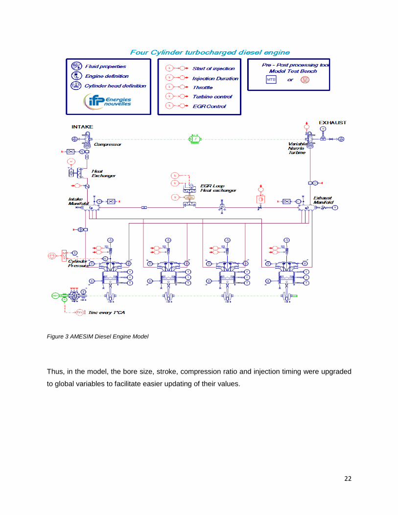
Figure 3 AMESIM Diesel Engine Model
Thus, in the model, the bore size, stroke, compression ratio and injection timing were upgraded
to global variables to facilitate easier updating of their values.
22

OBJECTIVE FUNCTION:
The objective function is:
minimize BSFC = Fuel_injected/P
CONSTRAINTS: The following constraints were implemented in the matlab optimization
code and the subsystem optimum was obtained.
1. The minimum power produced by the engine should be greater than 60kW which is typical
output of engines in hybrid vehicles.
2. The bore size (B) is limited by the weight of the engine. Higher weight reduces efficiency.
Also, larger bore size leads to larger engines. Also, larger bores lead to packaging
constraint. The constraint selected for this study was adopted from Heywood as bore size
must be between 75 mm and 100 mm
3. Compression ratio is limited by the maximum pressure that can be sustained in the
cylinder 17<CR<22. These constrains are dictated by the maximum pressures
[mechanical and thermal stresses] that can be sustained by the engine.
4. Stroke size (S) is limited by the bore to stroke ratio as 0.9<S/B<1.2. This, along with the
bore size gives a range of 67.5 mm to 120mm.
5. The mean piston speed must lie between 7m/s and 15 m/s
6. The injection timing must lie with the range -10 to 25 CAD BTDC to prevent low efficiencies
and high emissions
OVERALL MODEL:
minimize BSFC = f( CR, B,S, InjTiming)
subject to:
g1: B – 100 ≤ 0 g2: 75 – B ≤ 0 g3: S – 1.2*B ≤ 0 g4: 0.9*B – S ≤ 0 g5: CR - 22 ≤ 0 g6: 17 – CR ≤ 0 g7: Vp – 15 ≤ 0 g8: 7 – Vp ≤ 0 g9: -10- InjTiming ≤ 0 g10: InjTiming – 25 ≤ 0 g11: 60- P ≤ 0
23
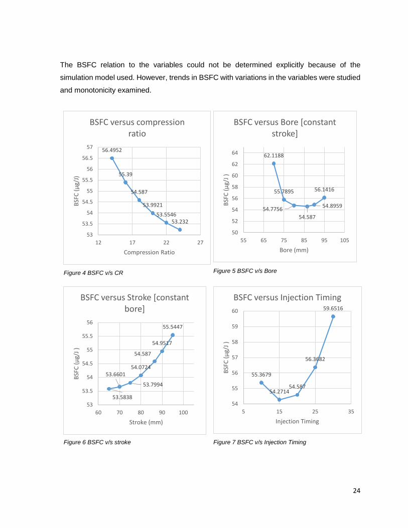
The BSFC relation to the variables could not be determined explicitly because of the
simulation model used. However, trends in BSFC with variations in the variables were studied
and monotonicity examined.
Figure 4 BSFC v/s CR
Figure 5 BSFC v/s Bore
Figure 6 BSFC v/s stroke
Figure 7 BSFC v/s Injection Timing
56.4952
55.39
54.587
53.9921
53.554653.232
53
53.5
54
54.5
55
55.5
56
56.5
57
12 17 22 27
BSFC
(µg/
J)
Compression Ratio
BSFC versus compression ratio
62.1188
55.7895
54.775654.587
54.8959
56.1416
50
52
54
56
58
60
62
64
55 65 75 85 95 105
BSFC
(µg/
J)
Bore (mm)
BSFC versus Bore [constant stroke]
53.5838
53.6601
53.7994
54.0724
54.587
54.9517
55.5447
53
53.5
54
54.5
55
55.5
56
60 70 80 90 100
BSFC
(µg/
J)
Stroke (mm)
BSFC versus Stroke [constant bore] 59.6516
56.3682
54.58754.2714
55.3679
54
55
56
57
58
59
60
5 15 25 35
BSFC
(µg/
J)
Injection Timing
BSFC versus Injection Timing
24

The graphs show that with increasing injection timing the BSFC first decreases till about 15 CAD
and then increases. With increasing compression ratio, the BSFC continues to decrease. This is
expected as higher compression ratios increase the thermal efficiency leading to improved BSFC.
With increase in bore, the BSFC decreases, until about 85mm. Thus using the above plots, the
behavior of BSFC with respect to the 4 variables was estimated.
MONOTONICITY TABLE:
B S CR InjTiming
Obj. Func. N/A N/A - N/A
g1 +
g2 -
g3 - +
g4 + -
g5 +
g6 -
g7 +
g8 -
g9 -
g10 +
Table 6 Engine Subsystem Monotonicity Analysis
Thus, every variable is bounded from above and below by at least one constraint. Thus the
problem is well bounded. Thus, the variation in BSFC with each of the four variables suggests
that the bore size can be expected to be the critical variable that dominates BSFC outcome. From
the trend analysis, it can be expected that constraint g5 would be an active constraint.
25

4. OPTIMIZATION RESULTS:
To carry out optimization of the engine subsystem, the AMESIM model was connected to Matlab
and fmincon solver was used. Initial trials with InteriorPoint Algorithm, the default option for
fmincon, failed to generate optimization results within reasonable time. That and the robustness
of SQP prompted us to pursue optimization using the DQP algorithm.
Results-
Table 7 Engine Subsystem Optimization Results
Sr.
No.
Initial Point Optimum
[ B , S , CR , InjTiming ]
Obj
Value
@initial
pt.
Objective
Value
(µg/j)
DiffMinChange
1 [80;81;18;9.7] [82.291;74.062;21.99;12.0752] 55.8627 53.4577 Default
2 [83;80;18;10]* [79.1099;79.459;22.0;12.1619] - 53.8598 Default
3 [82;84;19;12]* [81.369;74.65;22.0;14.17] - 53.4756 Default
4 [81;76;20;10] [81.8534;73.6691;22.0;13.25] 54.5269 53.3856 0.01
5 [83;79;20;12] [82.39;75.96;22.0;13.93] 54.5868 53.5058 0.01
6 [81;77;20;13] [82.16;73.94;22.0;13.64] 54.22 53.3906 0.01
7 [83;75;20;14] [82.41;74.38;21.999;13.8689] 54.0383 53.4077 0.05
8 [81;73;20;15] [81.83;73.65;22.0;13.6523] 54.0548 53.3875 0.05
9 [78;71;20;15] [80.36;72.33;22.0;12.2785] 54.4612 53.4204 0.05
10 [72;74;21;11] [82.1507;74.004;22.0;13.0585] 54.5152 53.3986 0.05
11 [82;72;21;12] [81.0487;72.94;22.0;12.3821] 53.6191 53.4028 0.05
12 [80;70;21;12] [79.8436;71.8593;22.0;11.891] 53.6639 53.4558 0.05
26

13 [90;90;21;20] [81.5299;73.383;21.99;13.242] 56.4775 53.3861 0.05
14 [90;90;20;0] [75.0;75.46;20.37;3.56] 61.7055 56.4641 0.05
15 [90;90;20;7] [80.797;72.71;21.99;12.49] 61.1078 53.4062 0.05
SUMMARIZED RESULT:
Bore = 81.85mm
Stroke = 73.669mm
CR = 22 Inj_Timing = 13.25
BSFC = 53.3856µg/J
Discussion of Results:
Since the variables were continuous, the gradient based optimization algorithm – fmincon was
used. An initial optimization exercise revealed that the system had multiple local minima. This
caused several problems in use of interior point algorithm. As a result, the interior point algorithm
was replaced by the SQP method. In addition the parameter DiffMinChange was used to vary the
minimum step size of SQP algorithm.
The problem of multiple local minima was handled by optimizing the subsystem from multiple
initial points. Thus, if the system reached the similar optimum even after starting from dissimilar
points, the optimum can be assumed to be a global minimum.
From the above table, it can be seen that the optimum result of 53.3856µg/J was obtained at
about bore size of 81.85mm, stroke size of 73.6691 mm, compression ratio of about 22 and
injection timing of 13.25 CAD BTDC. The slight variation in the optimum solution is attributed to
the existence of multiple local minima.
27

5. PARAMETRIC SWEEP:
CONSTRAINT RELAXATION: [RELAX LOWER BOUND]
Variation in Constraint on mean piston speed: Tightening the constraint
It was observed that the lower speed bound of 7m/s could become an active constraint if it was
tightened. Thus, the lower bound was progressively increased and its effect on the design
variables and objective function was observed.
Speed Constraint
Limit : Lower bound
Minimizer Objective
Value:
BSFC B(mm) S(mm) CR Injection
Timing
7 m/s 81.8534 73.6691 22 13.25 53.3856
7.5 m/s 82.9317 75 21.99 13.8345 53.4362
8 m/s 81.5188 80 22 14.3357 53.7934
8.5 m/s 79.5528 85 22 14.4456 54.1538
9 m/s 77.2047 90 22 14.4054 54.5139 Table 8 Engine Subsystem Constraint relaxation
The variation of BSFC and design variables with the constraint is shown below.
53
53.5
54
54.5
55
6 7 8 9 10
BSFC
Constraint lower limit
Objective v/s constraint
76
78
80
82
84
6 7 8 9 10
Bore
(mm
)
Constraint lower limit
Bore v/s speed constraint
28

Thus, as the constraint is relaxed, BSFC decreases. The compression ratio does not change with
the constraint. The optimum value of bore reaches a maximum at about a lower bound of 7.5m/s.
The stroke size decreases with relaxing the constraint. This is to be expected since the constraint
on mean piston speed binds the stroke. The injection timing does not show any significant trends.
The relaxation in mean piston speed constraint allows lower values of stroke size. This in turn
allows for smaller bore sizes (remember S/B is also limited) and bore size has an optimum around
82mm.
65
75
85
95
6 7 8 9 10
Stro
ke (m
m)
Constraint lower limit
Stroke v/s speed constraint
20
22
24
6 7 8 9 10
Com
pres
sion
Ratio
Constraint lower limit
Compression ratio v/s speed constraint
1313.5
1414.5
15
6 7 8 9 10Inje
ctio
n tim
ing
Constraint lower limit
Injection timing v/s speed constraint
29
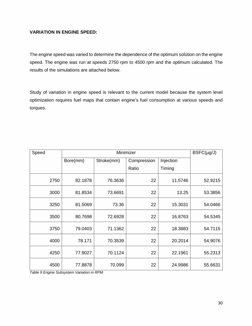
VARIATION IN ENGINE SPEED:
The engine speed was varied to determine the dependence of the optimum solution on the engine
speed. The engine was run at speeds 2750 rpm to 4500 rpm and the optimum calculated. The
results of the simulations are attached below.
Study of variation in engine speed is relevant to the current model because the system level
optimization requires fuel maps that contain engine’s fuel consumption at various speeds and
torques.
Speed Minimizer BSFC(µg/J)
Bore(mm) Stroke(mm) Compression
Ratio
Injection
Timing
2750 82.1878 76.3636 22 11.5746 52.9215
3000 81.8534 73.6691 22 13.25 53.3856
3250 81.5069 73.36 22 15.3031 54.0466
3500 80.7698 72.6928 22 16.8763 54.5345
3750 79.0403 71.1362 22 18.3883 54.7115
4000 78.171 70.3539 22 20.2014 54.9076
4250 77.9027 70.1124 22 22.1961 55.2313
4500 77.8878 70.099 22 24.9986 55.6631 Table 9 Engine Subsystem Variation in RPM
30

The variation of BSFC and design variables is shown below.
Thus, with increasing speed, the objective value steadily increases. The compression ratio is
largely unaffected as expected. The injection timing steadily advances with increasing speed. The
stroke and bore size reduces with increasing speed.
5253545556
2250 2750 3250 3750 4250 4750BSFC
(mic
ro-g
/J)
Speed(RPM)
Objective v/s speed
767880828486
2250 2750 3250 3750 4250 4750
Bore
(mm
)
Speed(RPM)
Bore v/s speed
0
10
20
30
2250 2750 3250 3750 4250 4750
Com
pres
sion
Ratio
Speed (RPM)
Compression Ratio v/s speed
65
70
75
80
85
2250 2750 3250 3750 4250 4750
Stro
ke(m
m)
Speed (RPM)
Stroke v/s speed
0
10
20
30
2250 2750 3250 3750 4250 4750Inje
ctio
n Ti
min
g
Speed (RPM)
Injection timing v/s speed
31

VARIATION IN MASS OF FUEL INJECTED [INJECTION DURATION]:
Tinj stands for injection duration i.e. time for which injector inserted the fuel
Tinj Injected Mass
(mg/cycle)
Minimizer Optimal
Value
(BSFC)
Bore(mm) Stroke(mm) CR Injection
Timing
0.0014 111.936 78.924 71.5121 22 9.5585 53.8157
0.0015 125.18 80.1108 72.5295 22 11.9395 53.5384
0.0016 139.8068 81.8534 73.6691 22 13.25 53.3856
0.0017 156.168 82.2277 74.005 22 15.0902 53.3395
0.0018 174.684 82.3001 75.9992 20.9995 14.2994 53.2118
0.0019 195.816 85.5179 77.179 21.2826 14.1272 52.6121 Table 10 Engine Subsystem Injection Duration Variation
The behavior of the design variables and objective function with the mass injected was plotted.
The graphs are shown below.
52.553
53.554
0.0013 0.0015 0.0017 0.0019 0.0021
BSFC
(mic
ro-g
/J)
Injection Duration
Objective v/s injection duration
78
80
82
84
86
0.0013 0.0015 0.0017 0.0019 0.0021
Bore
(mm
)
Injection Duration
Bore v/s injection duration
7072747678
0.0013 0.0015 0.0017 0.0019 0.0021
Stro
ke(m
m)
Injection Duration
Stroke v/s Injection Duration
20
22
24
0.0013 0.0015 0.0017 0.0019 0.0021
CR
Injection Duration
Compression ratio v/s Injection duration
32

Thus, with increasing mass of fuel injected, the objective function i.e. BSFC decreases. The bore
and stroke size increases to maintain the lower bsfc values. It is critical to note that at around
0.0016 to 0.0018 sec injection duration, the bore size essentially remains constant. This is
relevant operation wise under changing engine load conditions. The compression ratio variation
cannot be explained. The injection timing remains largely constant for injection durations greater
than the base case of 0.0016 sec.
CONCLUSION:
A BSFC optimum value of 53.3856µg/J is achieved. It is practical in the sense that all relevant
geometrical constraints on bore and stroke size have been specified. However, a study of engine
mechanical stresses and a study with a combustion model that can simulate the diffusion and
premixed burn would yield greater insight into the optimal result. But in the current domain of the
problem, the result is practical. The parametric tradeoffs are summarized below.
• At higher speeds, the engine friction losses increase, but the heat transfer losses decrease
because of lesser combustion duration. Thus, BSFC increases.
• Optimum value of compression ration remains unchanged with speed. This is expected
because increase in compression ratio leads to an increase in efficiency.
• Injection timing is advanced as speed is increased. The fuel injection is advanced because
of smaller ignition delay lesser time available for combustion.
• The relaxing of constraint on mean piston speed leads to a decrease in BSFC value. This
happens because a decrease in stroke size allows a decrease in bore size which has an
optimum about 82mm for the present model.
• The bore size is the variable that has the most impact on the BSFC
0
10
20
0.0013 0.0015 0.0017 0.0019 0.0021
Inje
ctio
n Ti
min
g
Injection Duration
Injection timing v/s injection duration
33
III) ELECTRICAL SUBSYSTEM 1. INTRODUCTION
ABOUT AMESIM
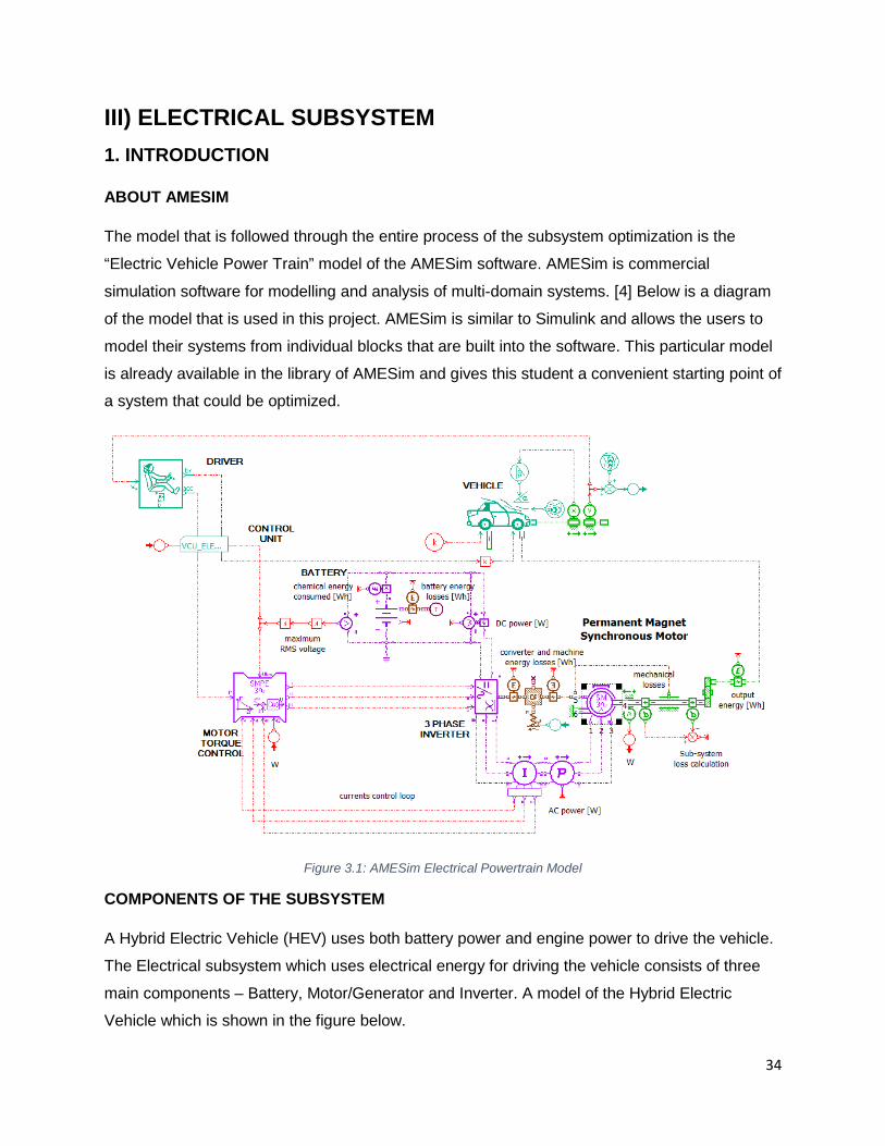
The model that is followed through the entire process of the subsystem optimization is the
“Electric Vehicle Power Train” model of the AMESim software. AMESim is commercial
simulation software for modelling and analysis of multi-domain systems. [4] Below is a diagram
of the model that is used in this project. AMESim is similar to Simulink and allows the users to
model their systems from individual blocks that are built into the software. This particular model
is already available in the library of AMESim and gives this student a convenient starting point of
a system that could be optimized.
Figure 3.1: AMESim Electrical Powertrain Model
COMPONENTS OF THE SUBSYSTEM
A Hybrid Electric Vehicle (HEV) uses both battery power and engine power to drive the vehicle.
The Electrical subsystem which uses electrical energy for driving the vehicle consists of three
main components – Battery, Motor/Generator and Inverter. A model of the Hybrid Electric
Vehicle which is shown in the figure below.
34

Figure 3.2:: Model of HEV
Battery
EV battery packs are assembled from connected battery cells and modules. The model of an
average electromechanical battery is given in the figure below. For this model the Open Circuit
Voltage (OCV) and the Internal Resistance (r) of the battery are assumed to be independent of
temperature influence. U is the output voltage across the terminals 1 and 2 and Cf is the filtering
Capacitance. The relationship between these variables is given by the equation
𝑑𝑑𝑑𝑑𝑑𝑑𝑑𝑑
= 𝐼𝐼2− 𝑑𝑑 − 𝑐𝑐𝑐𝑐𝑐𝑐
𝑟𝑟𝐶𝐶𝑓𝑓
Figure 3.3: Battery Representation
35

The performance of a battery is primarily defined by State of Charge (SoC), Nominal Capacity
and Specific Energy. The Open Circuit Voltage (ocv) and the internal resistance are dependent
on SoC and the number of cells in series. It is very important to maintain state of charge within
limits and it is assumed here that the AMESim model would ensure the limits are followed.
Nominal capacity defines the capacity of the battery in Ampere hours and is measured by
discharging the battery at a specific current from 100% SoC. [7] Specific Energy defines the
energy stored per unit mass and defines the size of the battery for delivering necessary power
requirements. The car battery market is currently dominated by Ni-MH (Nickel-Metal Hydride)
batteries and Lithium-ion batteries (Li-ion) and examples are shown below (source: internet).
Motor/Generator
The model for a motor used in HEV is shown in the figure below. The motors used in HEVs
have a requirement of high rate of acceleration and deceleration, high torque low speed hill
climbing, low torque high speed cruising and a wide speed range of operation. [5] Conceptually
motor and generator mode of operation will result in the same efficiency even though in actuality
there is some difference. Modern power electronics control the mode of operation of the motor.
The motor used in this case is a permanent magnet synchronous AC motor.
36

Figure 3.4: Motor Representation
As the motor can also act as a generator when power is supplied from the engine, it is important
to keep in mind the sign conventions of the directions and appropriately work on the model. The
below figure provides us with the details of motor related conventions used in the AMESim
Model.
Figure 3.5: AMESim Motor Conventions
Inverter
The model of the inverter used in the AMESim follows a continuous conduction mode. The
characteristics of the diodes and the transistors used are all assumed to be linear. As can be
seen from the figure 3.1, the current and voltage values to the motor/generator pass through the
inverter and hence the inverter is an important part of the subsystem. However, this project
37

does not focus on the inverter as the overall efficiency is far less dependent on the setting of the
individual components of the inverter model in AMESim.
PROBLEM DEFINITION
ASSUMPTIONS
The following list comprises of all the important assumptions made for the completion of this
project
• AMESim model is an accurate representation of the electrical sub-system of a hybrid
sedan car
• There are no spatial restrictions on the battery
• Upper and lower bounds on the battery cells reflect the weight and cost constraints
adequately. This student has not considered separate cost and weight constraints as the
bounds have been derived from previous project work that already took this into
consideration.
• Similarly, weight and cost limitations of the motor are reflected in the bounds of its
variables
• It is also assumed that there are no incongruities between AMESim model variable
values and actual physical range of variable values. So we assume there are no physical
limitations on variable values as long as AMESim allows them.
DESIGN PARAMETERS
The design parameters that are kept constant throughout the design optimization problem, after
identification of the variables, are as follows:
• A standard drive cycle has been used – The North European Drive Cycle (NEDC) is
used throughout the optimization process. This parameter is critical in determining the
bounds or the constraints, especially the power.
• The nominal voltage of each cell of the battery is kept at 6 volts. This is important for
determining the bounds on the voltage.
• Number of battery packs in parallel is taken as one.
• Motor/generator is a Permanent Magnet Synchronous machine with star (Y)
configuration
38

• The motor gear ratio is kept constant throughout the problem at 5. The output is
measured before the gear but this is still listed as a parameter as it might affect the
process maps generated for the system level optimization.
DESIGN VARIABLES
After starting with eight initial variables, mostly based on what the AMESim model allows to be
changed readily, the following four variables are selected as design variables based on the
amount of impact these variables have on the efficiency of the subsystem.
• Number of cells in series in the battery pack – Ns
The relationship between efficiency and Ns is shown in the graph below. It can been
seen that the efficiency increases till about 150 cells and stays more or less constant
thereafter. The upper and lower bounds for this variable are set at 150 cells and 50 cells
respectively. The limits are partly based on the below graph and partly on the weight
calculations performed in a previous project of Swetha Viswanatha [9].
• Number of pole pairs of the motor – P
The number of pole pairs in the motor has an impact on the efficiency of the subsystem.
They control the speed of the motor. The efficiency peaks at around 2 or 3 pole-pairs but
reduces as the pole-pairs increase. The upper and lower bounds on the pole-pairs is
taken to be 5 and 1 based on the limitation on the size of the motor that can be used in a
car system.
39

• Inductance of the stator winding – Ls
The next variable, also of the motor, is the inductance of the stator winding. The
efficiency of the model with increase in Ls increases monotonically. An inductance
represents a temporary storage of energy and one can see that as this goes up the
efficiency of the system goes up. The upper and lower bounds on this variable are
decided to be 0.006 Henry and 0.0015 Henry.
• Permanent Magnet Flux linkage of the motor – Phif The last of the design variables is the permanent magnet flux linkage of the motor. This
variable is responsible for the magnetic force developed in the motor. The efficiency
curve against this variable shows that the best efficiency value is achieved between 0.3
Weber and 0.4 Weber. The bounds on this variable are set between 0.5 Weber and 0.1
Weber.
40

CONSTRAINTS ON DESIGN VARIABLES
The AMESim model internally has many constraints that govern the physics of the variables
used. In addition to these variables the model also has error input constraints and limit
constraints. So, instead of setting constraints that might violate the model behaviour and
assumptions, this student has chosen to apply upper bounds on the voltage of the battery,
speed of the motor and have upper and lower bounds on the power of the motor. The bounds
on the power output of the motor also in turn control the power supplied by the battery due to
the closed loop nature of the system. One can see that the constraints are not directly on the
design variables but on intermediate variables which in turn are affected by the changes in the
design variables. The four constraints are listed below:
• Maximum Voltage of a battery <= Ns*6 V
• Maximum absolute speed <= 6500 RPM
• Maximum absolute power <= 60 KW
• Minimum absolute power >= 26 KW
OBJECTIVE FUNCTION
The objective function then is to maximize the efficiency of the electrical subsystem, measured
by the output energy of the motor divided by the input energy supplied by the battery. In the
model the output is measured by using the power value at a power sensor immediately after the
motor and then integrating it over the entire drive cycle. The input similarly is calculated by using
the open circuit voltage value of the battery for a given configuration, which changes based on
the value of Ns and the current output at the output port of the battery. The open circuit voltage
41

is considered in order to account for the losses due to internal resistance of the battery. The
equation used in AMESim model is given below.
𝜂𝜂 = ∫ (𝐵𝐵𝑐𝑐𝑑𝑑𝑐𝑐𝑟𝑟 𝑂𝑂𝑁𝑁𝑑𝑑𝑂𝑂𝑁𝑁𝑑𝑑 𝑃𝑃𝑐𝑐𝑤𝑤𝑒𝑒𝑟𝑟)𝑑𝑑𝑑𝑑𝑑𝑑𝑑𝑑𝑑𝑑 𝑐𝑐𝑐𝑐𝑐𝑐𝑐𝑐𝑑𝑑0 𝑑𝑑𝑑𝑑
∫ (𝐵𝐵𝑟𝑟𝑑𝑑𝑑𝑑𝑒𝑒𝑟𝑟𝑐𝑐 𝐼𝐼𝑐𝑐𝑂𝑂𝑁𝑁𝑑𝑑 𝑃𝑃𝑐𝑐𝑤𝑤𝑒𝑒𝑟𝑟)𝑑𝑑𝑑𝑑𝑑𝑑𝑑𝑑𝑑𝑑 𝑐𝑐𝑐𝑐𝑐𝑐𝑐𝑐𝑑𝑑0 𝑑𝑑𝑑𝑑
OPTIMIZATION PROBLEM
Bringing it all together, the optimization problem for the electrical subsystem is shown below.
f = minimize (- η), where η = f (Ns, P, Ls, Phif)
Subject to the constraints:
g1: V battery – Ns*6 <= 0
g2: Maximum absolute motor speed – 6500 <= 0
g3: Maximum absolute motor power – 60000 <= 0
g4: 26000 - Minimum absolute motor power <= 0
g5: 50-Ns <=0
g6: Ns-150 <= 0
g7: 1-P <= 0
g8: P-5 <= 0
g9: 0.0015-Ls <= 0
g10: Ls-0.006 <= 0
g11: 0.1-Phif <= 0
g12: Phif – 0.5 <= 0
42
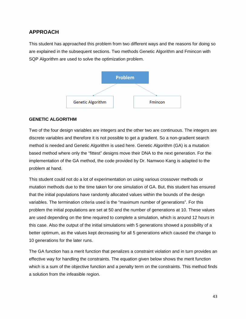
APPROACH
This student has approached this problem from two different ways and the reasons for doing so
are explained in the subsequent sections. Two methods Genetic Algorithm and Fmincon with
SQP Algorithm are used to solve the optimization problem.
GENETIC ALGORITHM
Two of the four design variables are integers and the other two are continuous. The integers are
discrete variables and therefore it is not possible to get a gradient. So a non-gradient search
method is needed and Genetic Algorithm is used here. Genetic Algorithm (GA) is a mutation
based method where only the “fittest” designs move their DNA to the next generation. For the
implementation of the GA method, the code provided by Dr. Namwoo Kang is adapted to the
problem at hand.
This student could not do a lot of experimentation on using various crossover methods or
mutation methods due to the time taken for one simulation of GA. But, this student has ensured
that the initial populations have randomly allocated values within the bounds of the design
variables. The termination criteria used is the “maximum number of generations”. For this
problem the initial populations are set at 50 and the number of generations at 10. These values
are used depending on the time required to complete a simulation, which is around 12 hours in
this case. Also the output of the initial simulations with 5 generations showed a possibility of a
better optimum, as the values kept decreasing for all 5 generations which caused the change to
10 generations for the later runs.
The GA function has a merit function that penalizes a constraint violation and in turn provides an
effective way for handling the constraints. The equation given below shows the merit function
which is a sum of the objective function and a penalty term on the constraints. This method finds
a solution from the infeasible region.
43

RESULTS OF GENETIC ALGORITHM
The plot shown below is the output of the final simulation of the GA method. The minimum
output value which is the result of all the mutations from the 50 initial populations is -0.80601.
The value of fval variable is also the same and this means that the penalty term is zero in the
above described equation. The maximum efficiency value output by the GA method is therefore
80.6% and this is given at the value of X where Ns = 150 cells, P = 5 pole-pairs, Ls = 0.004533
H and Phif = 0.2834 Wb. Number of cells and Ls are absolutely in line with the expectations but
the pole pairs are expected to be around 3, and Phif is expected to be around 0.35 when looked
at the performance of efficiency against individual variables alone. The output shows that the
best solution is not necessarily a combination of best individual variable values.
Figure 3.6: GA Result Plot
44

FMINCON WITH SQP ALGORITHM
Genetic Algorithm method is usually not used for finding the true optima and is a good method
for exploring the region. But, in this case no further analysis is done on the results of the genetic
algorithm and the optimum value returned by this method is cross-checked by a more robust
optimum finding method – fmincon with Sequential Quadratic Programming (SQP) algorithm. To
use this method, all four design variables are assumed to be continuous. As AMESim would not
allow one to make this assumption, a meta model is built using the output from AMESim and the
function and the constraints are estimated using the curve fitting app of matlab function
nnstart().
In order to build a meta-model, 625 samples are identified from the design space by dividing
each variable into 5 uniformly spaced values, thereby giving us 5X5X5X5 samples. Then the
AMESim model is used to output the actual function and constraint values for these 625
samples. Using these 625 samples, the neural network method is used with 10 hidden layer
neurons to train the data. As the sample size is small, the Bayersian Regularization algorithm is
used to train the data. The sample set is divided into 70% training data, 15% validation data and
15% testing data in order to check for proper generalization of the fitted curve.
The results of the curve fitting tool for the objective function values of the samples are shown
below. The curve fit is able to closely match the AMESim model as seen from the high R value
which is above 0.99 for both training and test data. The mean square error value is also very
low, here error representing the difference between the actual value and the estimate.
45

A similar approach for the four constraints is followed and the graphs for all four constraints
have a high R value. Therefore the function meta-model and the constraint meta-model are
close predictors of the actual AMESim model used but with the assumption that the variables
are all continuous. The regression graphs for the four constraints are shown below. The same
procedure is followed to generate the models of all the constraints with the same training set
ratios.
Power Maximum Constraint Power Minimum Constraint
Speed Maximum Constraint Voltage Maximum Constraint
Once the model is built, matlab is used for optimizing the variables using fmincon() for the
generated function and constraint meta-models. The results of the fmincon() method are
discussed next.
46

RESULTS OF FMINCON
The table below lists the optimum values of fmincon() for various starting values. The function
uses the SQP algorithm that is taught in class and is known to be a very robust algorithm in
finding an optimum solution. The optimum found through this method is not necessarily a global
optimum but the algorithm ensures a global convergence and therefore finds an optimum
solution from any initial point.
The output gives two solutions, one of which is closer to what the GA algorithm has given at
similar values of the minimizer to those obtained from GA. The other solution is a better one
than what GA has output. In the second case, the pole-pair value is 2.9769 which is not an
integer and when a integer value closer to it, i.e. , 3 is used along with the other minimizer
values in AMESim the output is shown to be 0.8051, which is lower than the optimum returned
by GA. The number of cells is always at 150 in both the cases and for all the different solutions
of the output. This is the only variable of the battery component and it is expected to hit the
upper end of the bound from the initial analysis.
FINAL RESULTS
Fmincon() has in a way helped us cross-check the output of the GA method but there is still no
guarantee that the output is a global minimum. Nevertheless, the result of the optimization is
better than the efficiency that was being returned by the model before the optimization. The
value of efficiency has increased by 5.4% (80.6% - 75.2%) as shown in the table below.
47

SENSITIVITY ANALYSIS – FOR SYSTEM OPTIMIZATION
In order to perform system level optimization all the variables of the subsystem are normally
considered. But because of time constraints, it is decided that the most important design
variable will be identified and maps corresponding to this variable would be generated for
system level optimization. In order to perform this analysis, the value of each of the solution is
moved to the next possible value or 1%, whichever is higher, and the corresponding change in
the function value from optimum is measured. The variable exhibiting the maximum change in
the function value is selected and in this case it is the permanent magnet flux linkage (Phif).
GENERATION OF MAPS
Map generation exercise is about identifying the efficiency values at different levels of the
design variable, over the range of speed and torque values of the motor. The speed and torque
values are discretized arbitrarily but at almost equal intervals and using the AMESim model
shown below, the efficiency values are calculated for 5 different levels of Phif, in the feasible
region. A new model in AMESim is created with the battery, inverter, the motor and the SMPE.
The torque value is set through the SMPE and the speed value is directly set at the motor. A
Matlab script is then used to pass the combination of values to compute the efficiency maps
automatically.
48

Figure 3.8: AMESim model for map generation
The efficiency calculated here is just that of the motor and the inverter and therefore the values
are higher than overall values by almost 15%. The maps generated are shown below. The map
at the optimizer Phif is steeper than the other maps. The maps shown here are only for the
motor region of operation and the efficiency values are assumed to be similar for the generator.
Figure 3.9: Maps of Phif for System Optimization
49

CONCLUSION OF ELECTRICAL SUBSYSTEM
After going through the experience of this project this student now have a better understanding
of how to approach an optimization problem. In retrospect there are a few things this student
would have liked to do differently. He should have been more proactive in thinking about the
problem earlier. At that time it was too overwhelming and seemed very confusing. A little effort a
little earlier in the project would have allowed him time for doing a few things which he now feels
he should have done. Like, doing parametric analysis to understand the effect of the various
parameters chosen to be constant throughout the problem. Sensitivity analysis of the
constraints to understand how the optimum value changes with change in the constraints.
Lastly, this student would have liked to repeat the exercise with more initial populations and
more generations. This project has given me a flavour of how complex and time-consuming an
optimization problem could be and for that he is thankful.
ACKNOWLEDGEMENTS
This student would sincerely like to thank Dr. Alparslan Emrah Bayrak, the team project advisor,
for being so helpful throughout the project. This project taught this student a lot about Design
Optimization and that learning would have been completely missing had it not been for the
continuous support of Dr. Bayrak, who helped this student cross many roadblocks along the
way.
In the process of doing this project, previous projects of Swetha Viswanatha [9] and Archit
Rastogi [8] both on battery systems are referred to and some ideas are derived from there.
50

IV) TRANSMISSION SUBSYSTEM 1 PROBLEM STATEMENT The power split transmission system will use one planetary gear and Final drive to couple the power from engine, motor and generator to the vehicle. In the actual planetary device there are 3 different gear sizes: planet gears, sun gear and ring gear. Planetary gear has one degree of freedom corresponding to torques i.e the torques for other two gears can be calculated if the torque of one gear is known .Also, the planetary has two degrees of freedom corresponding to the rotational speed. According to the driving cycle, the torque required by vehicles can be known and the torque to sun and ring gear can be evaluated. According to that torques, both motor and engine have optimal operating points. So, a trade-off is needed to maximise the fuel economy.
2 ASSUMPTIONS The number of ring gears, sun gears and planetary gears are considered to be continuous for the problem instead of discrete values. The inertia of sun gear, ring gear and planetary gear is very small compared to other values .So, it is considered to be zero in the problem .The vehicle is considered to have same generator and battery as of THS II.
3 NOMENCLATURE Symbol Description Units Value
sI Inertia of sun gear Kg.m^2 0
cI Inertia of carrier gear Kg.m^2 0
rI Inertia of ring gear Kg.m^2 0
mI Inertia of motor Kg.m^2 0.0226
gI Inertia of generator Kg.m^2 0.0226
eI Inertia of Engine Kg.m^2 0.18
R No. of ring gears - -
S No. of sun gears - -
K Final Drive Ratio - -
F Friction force between gear tooth F -
ρ Density of air Kg.m^3 1.2
A Frontal Area m^2 2.1840
rf Rolling resistance coefficient - 0.015
51
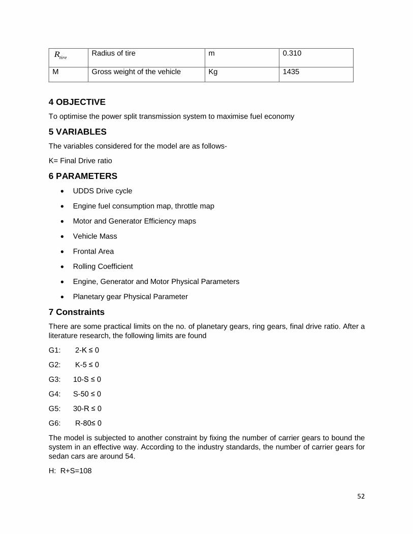
tireR Radius of tire m 0.310
M Gross weight of the vehicle Kg 1435
4 OBJECTIVE To optimise the power split transmission system to maximise fuel economy
5 VARIABLES The variables considered for the model are as follows-
K= Final Drive ratio
6 PARAMETERS • UDDS Drive cycle
• Engine fuel consumption map, throttle map
• Motor and Generator Efficiency maps
• Vehicle Mass
• Frontal Area
• Rolling Coefficient
• Engine, Generator and Motor Physical Parameters
• Planetary gear Physical Parameter
7 Constraints There are some practical limits on the no. of planetary gears, ring gears, final drive ratio. After a literature research, the following limits are found
G1: 2-K ≤ 0
G2: K-5 ≤ 0
G3: 10-S ≤ 0
G4: S-50 ≤ 0
G5: 30-R ≤ 0
G6: R-80≤ 0
The model is subjected to another constraint by fixing the number of carrier gears to bound the system in an effective way. According to the industry standards, the number of carrier gears for sedan cars are around 54.
H: R+S=108
52
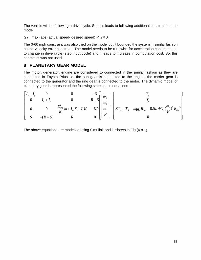
The vehicle will be following a drive cycle. So, this leads to following additional constraint on the model
G7: max (abs (actual speed- desired speed))-1.7≤ 0
The 0-60 mph constraint was also tried on the model but it bounded the system in similar fashion as the velocity error constraint. The model needs to be run twice for acceleration constraint due to change in drive cycle (step input cycle) and it leads to increase in computation cost. So, this constraint was not used.
8 PLANETARY GEAR MODEL The motor, generator, engine are considered to connected in the similar fashion as they are connected in Toyota Prius i.e. the sun gear is connected to the engine, the carrier gear is connected to the generator and the ring gear is connected to the motor. The dynamic model of planetary gear is represented the following state space equations-
22 3
0 00 0
0.5 ( )0 0
0( ) 0
s g gg
c e ee
rtirer m fb r tire d tirem r
I I S TI I R S T
R KT T mgf R AC Rm I K I K KRKK FS R S R
ωω
ωω ρ
+ − + + = − − −+ + − − +
The above equations are modelled using Simulink and is shown in Fig (4.8.1).
53

Figure 8 Simulink model of planetary gear subsystem
This planetary gear system is subsystem of vehicle system. So, this needs to have a vehicle model with control strategy. The vehicle model integrated with rule based control strategy shown in Figure 8 will be used for initial analysis.
The control strategy model will be optimised using ECMS algorithm. An engine map, and motor map will be fed as parameters .The vehicle will be following UDDS Drive cycle .So, the gear ratio will be optimised in such a way that the engine and motor will operate in high efficiency zones.
54
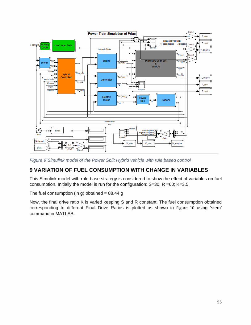
Figure 9 Simulink model of the Power Split Hybrid vehicle with rule based control
9 VARIATION OF FUEL CONSUMPTION WITH CHANGE IN VARIABLES This Simulink model with rule base strategy is considered to show the effect of variables on fuel consumption. Initially the model is run for the configuration: S=30, R =60; K=3.5
The fuel consumption (in g) obtained = 88.44 g
Now, the final drive ratio K is varied keeping S and R constant. The fuel consumption obtained corresponding to different Final Drive Ratios is plotted as shown in Figure 10 using ‘stem’ command in MATLAB.
55

Figure 10 Variation in fuel consumption corresponding to variation in Final Drive Ratio
Figure 11 Variation in fuel consumption corresponding to variation in No. of sun gears
Similarly, the variation in fuel consumption is plotted against the variation in no. of sun gears, keeping K and R fixed and is shown by Figure 11
56

Figure 12 Variation in fuel consumption corresponding to variation in No. of ring gears
The variation in fuel consumption is plotted against the variation in no. of ring gears, keeping K and S fixed and is shown by Figure 12
It can be concluded from the above plots that the final drive ratio, no. of sun gears, no. of planetary gears are good design variables and they can be optimised within the constraints to obtain maximum fuel economy.
10 MODEL OPTIMISATION The Simulink model used above uses rule based control strategy and this is not an optimal control strategy. So, the model is initially designed for optimal control by developing a cost Hamiltonian and optimising it using PMP principles. There is an approximation to PMP technique called ECMS technique that is used for optimising control strategy.
ECMS
The Equivalent consumption minimization strategy is based on the concept of instantaneous equivalent fuel consumption. It is calculated by defining an equivalent total fuel consumption as
( ). .
( ) ( ) *fequi feng fbattm t m f SOC m= + Equation 1
Where
/ _fbatt eng battm SC P Eff batt= Equation 2
In Equation (1) mfbatt represents the equivalent fuel consumption of the electric power. The average engine fuel consumption SCeng is selected based on the engine fuel map. Similarly, the average power efficiency of the motor/generator Eff_batt is selected from its efficiency map. This results in an approximated equivalent fuel consumption value regardless of the speed and torque of the engine and the motor/generator. Therefore, Equation (1) is only an approximation. f(soc) is
57

a weighting factor (Figure 13) to achieve SOC regulation. It sets the target SOC at around 0.6 and weights the SOC away from this target value by varying the additional weight f (soc).
Figure 13 Plot of f (SOC) with variation in SOC
Given a driver power demand, the optimal engine power can be calculated by comparing all the possible solutions and select the engine power that achieves minimal equivalent fuel consumption. The calculated optimal engine power map is determined offline and is as shown in Figure 14. This map is implemented as part of the power management controller as shown in Figure 15
58

Figure 14 Surface plot for Engine optimal power obtained by using ECMS
Figure 15 ECMS control implemented in Power Management of the Simulink Model
59

ECMS algorithm optimised the control strategy. So, the final model is obtained by integration of 2D look up tables obtained from the ECMS algorithm.
11 SUBSYSTEM OPTIMISATION There are 3 variables in the system. The number of ring gears variable is eliminated by using the equality constraint H .This leads to two variables in the system. The Simulink model is initialised from MATLAB file .So, a model function for MPG and velocity error constraint is created for the two variables that can be called by another function. SQP algorithm with fmincon is used to optimise the subsystem in MATLAB. As the Simulink model takes value from the default MATLAB workspace and we made the file as model function, So, the Simulink model was not able to take values from the workspace as the anything defined inside the function does not get saved in the default workspace. The following command is used to solve this problem-
options = simset('SrcWorkspace','current');
sim ('Model',[],options);
The system is run for different values different initial conditions and the optimized values are obtained as shown in Table 11.
Initial values [S, K]
Xopt [Sopt,Kopt]
Ropt=108- Sopt MPG
[30 3.5] [28.91 2.96] 79.09 50.6473
[19 3] [28 2.49] 80 50.1546
[18 3.5] [27.96 2.54] 80.04 50.2816
[24 2.8] [28.82 3.04] 79.18 50.7028
[40 5] [28.55 3.29] 79.45 50.7038
Table 11 Subsystem Optimization results
12 RESULT DISCUSSION It can be concluded from the Table 4.11.1 that the optimum values xopt = [28.55 79.45 3.29] and the maximum MPG is 50.7038 as all the results for different initial conditions are really close. This optimum value is obtained by assuming variables to be discrete ad this optimum value is within constraint limits. This optima is obtained at constant maps for engine, generator and motor .This optima can be varied by changing the maps for engine motor and generator and this will be done in the system level optimisation.
60
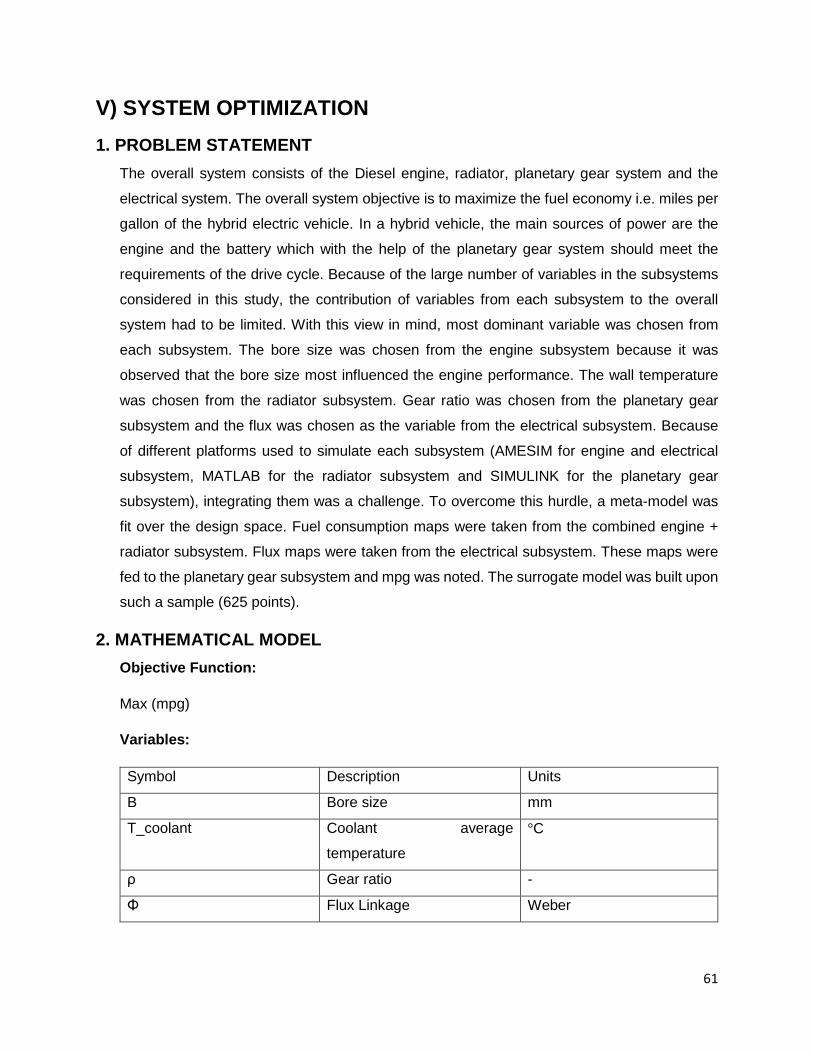
V) SYSTEM OPTIMIZATION 1. PROBLEM STATEMENT
The overall system consists of the Diesel engine, radiator, planetary gear system and the
electrical system. The overall system objective is to maximize the fuel economy i.e. miles per
gallon of the hybrid electric vehicle. In a hybrid vehicle, the main sources of power are the
engine and the battery which with the help of the planetary gear system should meet the
requirements of the drive cycle. Because of the large number of variables in the subsystems
considered in this study, the contribution of variables from each subsystem to the overall
system had to be limited. With this view in mind, most dominant variable was chosen from
each subsystem. The bore size was chosen from the engine subsystem because it was
observed that the bore size most influenced the engine performance. The wall temperature
was chosen from the radiator subsystem. Gear ratio was chosen from the planetary gear
subsystem and the flux was chosen as the variable from the electrical subsystem. Because
of different platforms used to simulate each subsystem (AMESIM for engine and electrical
subsystem, MATLAB for the radiator subsystem and SIMULINK for the planetary gear
subsystem), integrating them was a challenge. To overcome this hurdle, a meta-model was
fit over the design space. Fuel consumption maps were taken from the combined engine +
radiator subsystem. Flux maps were taken from the electrical subsystem. These maps were
fed to the planetary gear subsystem and mpg was noted. The surrogate model was built upon
such a sample (625 points).
2. MATHEMATICAL MODEL Objective Function:
Max (mpg)
Variables:
Symbol Description Units
B Bore size mm
T_coolant Coolant average
temperature
°C
ρ Gear ratio -
Φ Flux Linkage Weber
61

Parameters
Symbol Description Value Units
CR Compression ratio 22 --
InjTiming Injection Timing 13.25 CAD BTDC
Ncyl Number of cylinders 4 --
T_fuel Fuel temperature 293 K
Q Heat rejection 80 KW
Bh, Bw, Bt Radiator dimensions [0.3,0.3,0.025] m
K Final drive ratio 3.29 -
Ns Cells in series 150 -
P Number of pole-pairs 5 -
Ls Stator Inductance 0.004533 H
Constraints:
A total of five constraints were chosen. One for bounding each of the four variables and one
constraint which limited the error in velocity as the hybrid vehicle followed the drive cycle.
g(1)= B- 95 ≤0
g(2)= -B+75≤0
g(3)= T_coolant - 205≤0
g(4)= -T_coolant+ 165≤0
g(5)= ρ -5 ≤0
g(6)= - ρ +2≤0
g(7)= Φ -0.5≤0
g(8)= -Φ+ 0.2834≤0
3. SYSTEM MODELLING
25 fuel consumption maps from engine-radiator, 5 efficiency maps from the motor and 5 change
in the gear ratio were fed into the vehicle model to get MPG values and velocity constraint values
from the vehicle model. The MPG values were obtained for different 625 combinations of 4 system
62

variables (See Apendix) and the metamodel was created for the system using neural networks.
The R value obtained for the model was found out to be 0.99.
4. OPTIMIZATION RESULTS The metamodel is optimized using ‘SQP algorithm with fmincon in MATLAB and the optimum
values are listed in Table 12
initial values B_opt T_opt Ρ_opt Ф_opt mpg_opt [80,180,0.35,4] 85.2029 182.8967 2.5662 0.5000 -62.3011 [100,205,0.29,2] 91.1812 205.0000 2.5662 0.5000 -61.7334 [95,205,0.29,2] 86.3540 205.0000 2.5621 0.4948 -66.1849 [85,165,0.5,2] 85.2029 182.8967 2.5662 0.5000 -62.3011 [85,225,0.5,2] 85.2029 182.8967 2.5662 0.5000 -62.3011 [90,185,0.4,4] 85.2029 182.8966 2.5662 0.5000 -62.3011 [80,195,0.5,3.3] 86.3540 205.0000 2.5621 0.4948 -66.1849 [82,191,0.37,3.8] 85.2029 182.8967 2.5662 0.5000 -62.3011 [87,198,0.47,4.46] 86.3540 205.0000 2.5621 0.4948 -66.1849 [94,188,0.44,5] 85.2029 182.8967 2.5662 0.5000 -62.3011
Table 12 System level optimization
It can be concluded from the Table that there are various local minima in the model and the global
minimum is [85.2029 182.8967 2.5621 0.5] and the optimum value of MPG is 66.1849.
5. SYSTEM ANALYSIS The following regression analysis in R shows that all the variables considered in the analysis are significant
63

6 CONCLUSION MPG value obtained from the system level optimization was found out to be 66.1849,which is
good enough for industry standards. Thus, it can be concluded from the project that fuel economy
of the vehicle can be optimized by optimizing the radiator, engine, electrical driveline and
Transmission System.
BSFC Maps:
Below are three representative examples of the BSFC maps that were constructed.
Bore: 75mm and Wall temperature = 165 °C
64
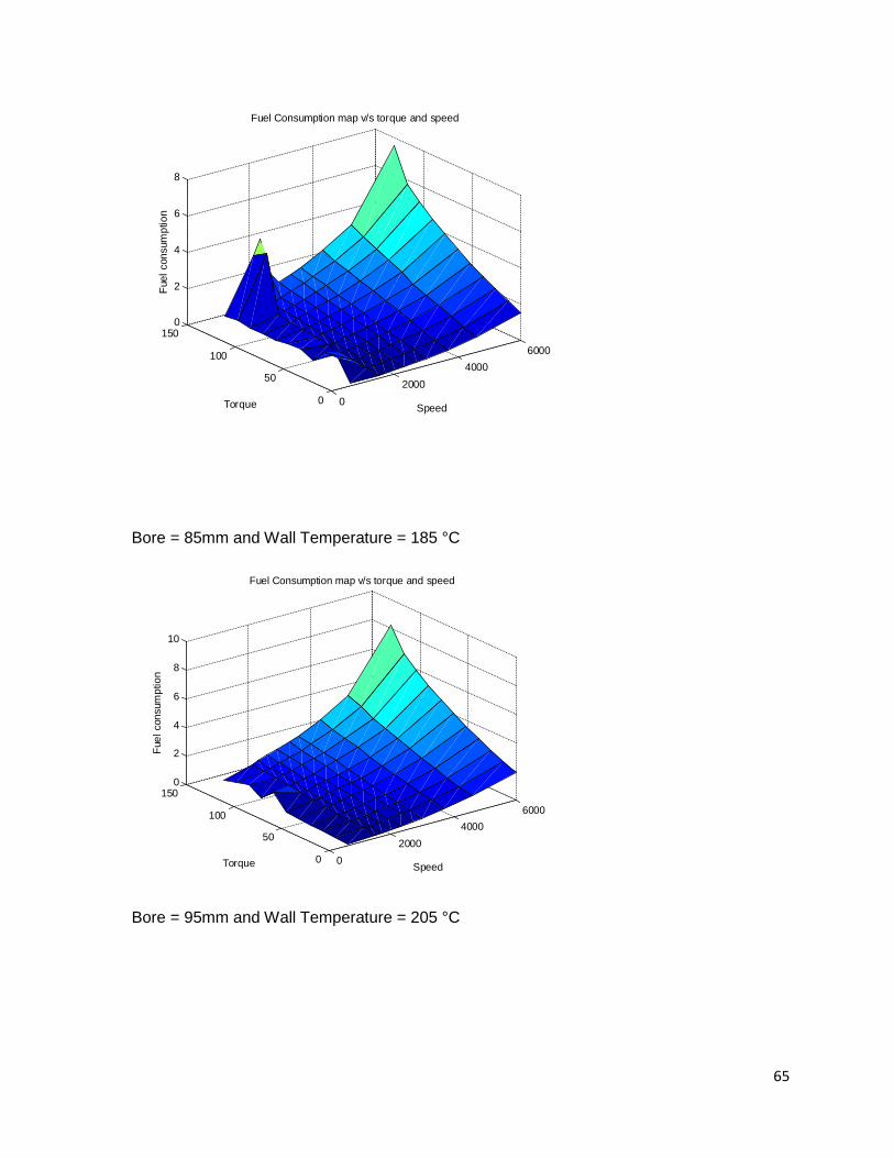
Bore = 85mm and Wall Temperature = 185 °C
Bore = 95mm and Wall Temperature = 205 °C
02000
40006000
0
50
100
1500
2
4
6
8
Speed
Fuel Consumption map v/s torque and speed
Torque
Fuel
con
sum
ptio
n
02000
40006000
0
50
100
1500
2
4
6
8
10
Speed
Fuel Consumption map v/s torque and speed
Torque
Fuel
con
sum
ptio
n
65

02000
40006000
0
50
100
1500
5
10
15
Speed
Fuel Consumption map v/s torque and speed
Torque
Fuel
con
sum
ptio
n
66

VI) REFERENCES [1]. E Y Ng, P W Johnson,S Watkins1 An analytical study on heat transfer performance of
radiators with non-uniform airflow distribution. DOI: 10.1243/095440705X35116
[2] Theodore L. Bergman, Frank P. Incropera, Adrienne S. Lavine Fundamentals of heat and mass
transfer 7th Edition.
[3] Heywood J.B. “Internal Combustion Engines fundamentals,” New York: McGrawHill, 1988
[4] AMESim. (n.d.). Retrieved April 22, 2015, from http://en.wikipedia.org/wiki/AMESim
[5] (n.d.). Retrieved April 22, 2015, from http://www.uotechnology.edu.iq/dep-
eee/lectures/3rd/Electrical/Machines 2/III_SM.pdf
[6] (n.d.). Retrieved April 22, 2015, from
http://www.nrel.gov/transportation/energystorage/pdfs/long_beach_btm.pdf
[7] (n.d.). Retrieved April 22, 2015, from
http://web.mit.edu/evt/summary_battery_specifications.pdf
[8] Previous Project - Rastogi, A. (2012). Optimal Design of Hybrid Electric Vehicle for Fuel Economy
[9] Previous Proejct - Viswanatha, S. (2014). Combining battery and ultra capacitor in parallel in a
pure electric vehicle. In Final Report.
67

VI) APPENDIX A) MATLAB CODE – Radiator Subsystem (SHUBHAM KHADRIA) Code for optimization
%% initial values x0=[10 1 0.2 0.006146 3 0.03 0.003 423.15 ]; % x0(1)=7; %No. of coolant tubes in one row ## To be varied % x0(2)=1; %No. of rows of tube in the core depth % x0(3)= 0.20; %Coolant tube length (m) ## equals the width of the core % x0(4)=(6.146*10^-3)*2; %Fin Height (m) ## to be varied % x0(5)=3; %No. of Profiles ## ## No of fins in the depth direction per coolant tube % %x0(8)=0.001; %Louvre Pitch (m)## ## to be varied % % x0(6)=0.005;% Fin material thickness; % x0(6)=0.03; %Fin width (m)## to be varied % x0(7)=0.003; %coolant tube cross section width (m) ## fixed very small value % x0(8)= 273.15+200; opt=2; %A=[];B=[]; Aeq=[];Beq=[];Lb=[];Ub=[]; if opt==1 OPTION= optimoptions('fmincon','Algorithm','sqp'); end if opt==2 OPTION= optimoptions('fmincon','Algorithm','active-set'); else OPTION=[]; end [x,fval,exitflag,output, lambda]= cheap_optim(x0, OPTION); [T,m]= objective(x); function [x,f,eflag, output, lambda] = cheap_optim(x0, opts) if nargin == 1 % No options supplied opts = []; end xLast = []; % Last place model was called myf = []; % Use for objective at xLast myc = []; % Use for nonlinear inequality constraint myceq = []; % Use for nonlinear equality constraint fun =@objfun; % the objective function cfun = @constr; % the constraint function [x,f,eflag, output, lambda] = fmincon(fun,x0,[],[],[],[],[],[],cfun,opts); function f = objfun(x) if ~isequal(x,xLast) [myf, myc] = objective(x); xLast = x; end f = myf;
68
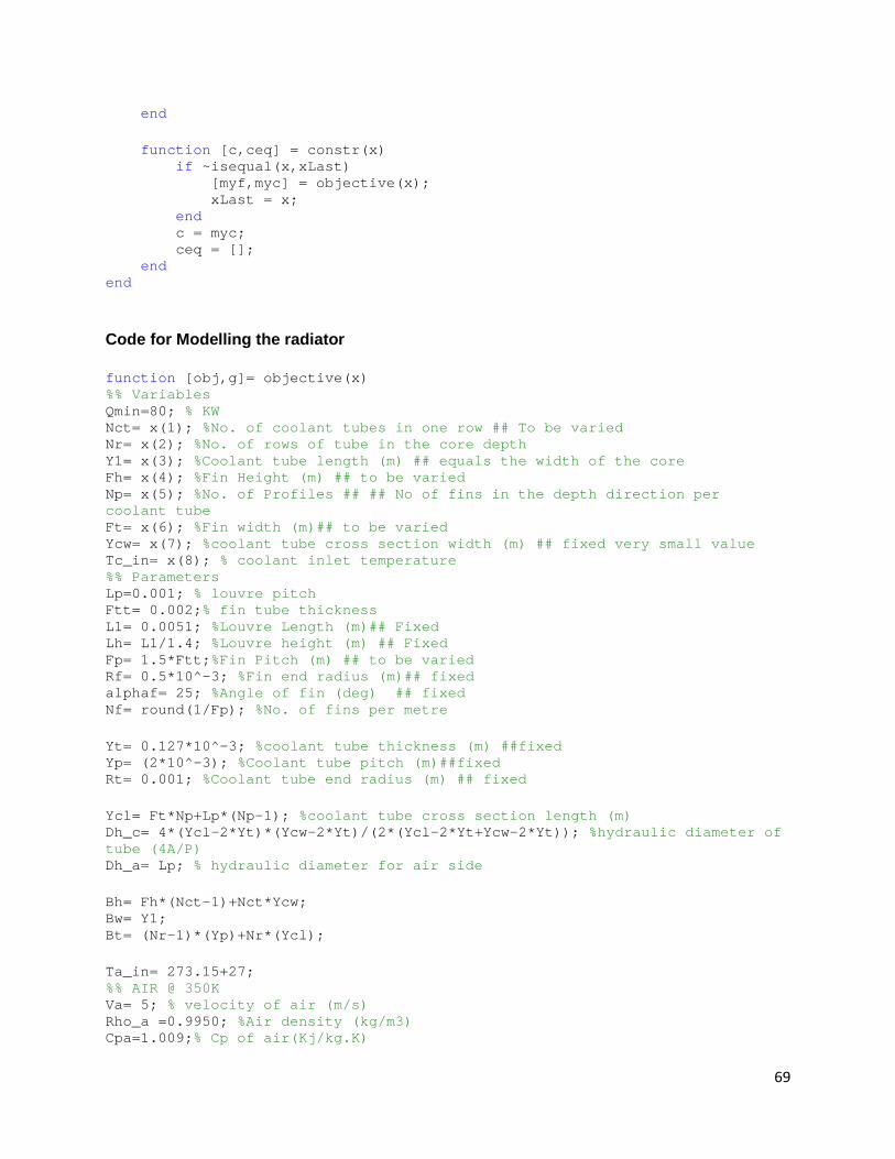
end function [c,ceq] = constr(x) if ~isequal(x,xLast) [myf,myc] = objective(x); xLast = x; end c = myc; ceq = []; end end Code for Modelling the radiator
function [obj,g]= objective(x) %% Variables Qmin=80; % KW Nct= x(1); %No. of coolant tubes in one row ## To be varied Nr= x(2); %No. of rows of tube in the core depth Y1= x(3); %Coolant tube length (m) ## equals the width of the core Fh= x(4); %Fin Height (m) ## to be varied Np= x(5); %No. of Profiles ## ## No of fins in the depth direction per coolant tube Ft= x(6); %Fin width (m)## to be varied Ycw= x(7); %coolant tube cross section width (m) ## fixed very small value Tc_in= x(8); % coolant inlet temperature %% Parameters Lp=0.001; % louvre pitch Ftt= 0.002;% fin tube thickness L1= 0.0051; %Louvre Length (m)## Fixed Lh= L1/1.4; %Louvre height (m) ## Fixed Fp= 1.5*Ftt;%Fin Pitch (m) ## to be varied Rf= 0.5*10^-3; %Fin end radius (m)## fixed alphaf= 25; %Angle of fin (deg) ## fixed Nf= round(1/Fp); %No. of fins per metre Yt= 0.127*10^-3; %coolant tube thickness (m) ##fixed Yp= (2*10^-3); %Coolant tube pitch (m)##fixed Rt= 0.001; %Coolant tube end radius (m) ## fixed Ycl= Ft*Np+Lp*(Np-1); %coolant tube cross section length (m) Dh_c= 4*(Ycl-2*Yt)*(Ycw-2*Yt)/(2*(Ycl-2*Yt+Ycw-2*Yt)); %hydraulic diameter of tube (4A/P) Dh_a= Lp; % hydraulic diameter for air side Bh= Fh*(Nct-1)+Nct*Ycw; Bw= Y1; Bt= (Nr-1)*(Yp)+Nr*(Ycl); Ta_in= 273.15+27; %% AIR @ 350K Va= 5; % velocity of air (m/s) Rho_a =0.9950; %Air density (kg/m3) Cpa=1.009;% Cp of air(Kj/kg.K)
69
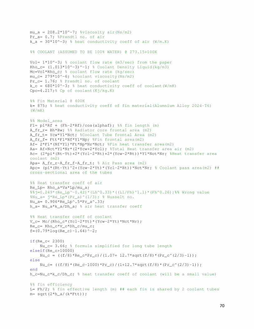
mu_a = 208.2*10^-7; %viscosity air(Ns/m2) Pr_a= 0.7; %Prandtl no. of air k_a = 30*10^-3; % heat conductivity coeff of air (W/m.K) %% COOLANT (ASSUMED TO BE 100% WATER) @ 273.15+100K Vol= 1*10^-3; % coolant flow rate (m3/sec) from the paper Rho_c= (1.013*10^-3)^-1; % Coolant Density Liquid(kg/m3) Mc=Vol*Rho_c; % coolant flow rate (kg/sec) mu_c= 279*10^-6; %coolant viscosity(Ns/m2) Pr_c= 1.76; % Prandtl no. of coolant k_c = 680*10^-3; % heat conductivity coeff of coolant(W/mK) Cpc=4.217;% Cp of coolant(Kj/kg.K) %% Fin Material @ 400K k= 875; % heat conductivity coeff of fin material(Alumnium Alloy 2024-T6) (W/mK) %% Model_area F1= pi*Rf + (Fh-2*Rf)/cos(alphaf); %% fin length (m) A_fr_r= Bh*Bw; %% Radiator core frontal area (m2) A_fr_t= Ycw*Y1*Nct; %Coolant Tube frontal Area (m2) A_fr_f= Ftt*F1*Nf*Y1*Np; %Fin frontal area(m2) Af= 2*F1*(Nf*Y1)*Ft*Np*Nr*Nct; %Fin heat transfer area(m2) Aa= Af+Nct*Y1*Nr*(2*Ycw+2*Ycl); %Total Heat transfer area air (m2) Ac= (2*pi*(Rt-Yt)+2*(Ycl-2*Rt)+2*(Ycw-2*Rt))*Y1*Nct*Nr; %Heat transfer area coolant (m2) Apa= A_fr_r-A_fr_f-A_fr_t; % Air Pass area (m2) Apc= (pi*(Rt-Yt)^2+(Ycw-2*Yt)*(Ycl-2*Rt))*Nct*Nr; % Coolant pass area(m2) ## cross-sectional area of the tubes %% Heat transfer coeff of air Re_Lp= Rho_a*Va*Lp/mu_a; %%j=0.249*(Re_Lp^-0.42)*(Lh^0.33)*((L1/Fh)^1.1)*(Fh^0.26);%% Wrong value %Nu_a= j*Re_Lp*(Pr_a)^(1/3); % Nusselt no. Nu_a= 0.906*Re_Lp^.5*Pr_a^.33; h_a= Nu_a*k_a/Dh_a; % air heat transfer coeff %% Heat transfer coeff of coolant V_c= Mc/(Rho_c*(Ycl-2*Yt)*(Ycw-2*Yt)*Nct*Nr); Re_c= Rho_c*V_c*Dh_c/mu_c; f=(0.79*log(Re_c)-1.64)^-2; if(Re_c< 2300) Nu_c= 3.66; % formula simplified for long tube length elseif(Re_c>10000) Nu_c = ((f/8)*Re_c*Pr_c)/(1.07+ 12.7*sqrt(f/8)*(Pr_c^(2/3)-1)); else Nu_c= ((f/8)*(Re_c-1000)*Pr_c)/(1+12.7*sqrt(f/8)*(Pr_c^(2/3)-1)); end h_c=Nu_c*k_c/Dh_c; % heat transfer coeff of coolant (will be a small value) %% fin efficiency L= Fh/2; % fin effective length (m) ## each fin is shared by 2 coolant tubes m= sqrt(2*h_a/(k*Ftt));
70

n_f= tanh((m*L))/(m*L); %fin Efficiency n_o= 1-Af/Aa*(1-n_f); %total Efficiency effect= sqrt(k*2/h_a/Ftt); % Fin effectivness %% Overall Heat transfer coeff. U= 1/A_fr_r*(1/(n_o*h_a*Aa)+1/(h_c*Ac))^-1; % Neglecting wall thickness and fouling resistance Ca= Rho_a*Va*Aa*Cpa; Cc= Mc*Cpc; if(Ca<Cc) Cmin= Ca; Cmax= Cc; else Cmin= Cc; Cmax= Ca; end NTU=U*A_fr_r/(Cmin*1000);%% Watt/Watt Cr=Cmin/Cmax; E= 1-exp(1/Cr*NTU^0.22*(exp(-Cr*NTU^0.78)-1)); Q= E*Cmin*(Tc_in-Ta_in); %(KW) %obj= -(Q/(Bh*Bw*Bt)); %obj= -Q; Tc_out= -Q/(Cc)+ Tc_in; Ta_out= Q/Ca+Ta_in; obj= Tc_out; %% constraints (inequality) g(1)=Bw-0.30; %0.4 g(2)=Bh-0.30; g(3)=Bt-0.025;%0.04 g(4)=-Nct+2; g(5)=-Nr+1; g(6)=-Y1+0.01; g(7)=-Fh+0.005; g(8)=-Np+1; g(9)=-Ft+0.005; %g(10)= -NTU+ 2.5; g(10)= -effect+2; g(11)=-Bw+0.01; g(12)=-Bh+0.01; g(13)=-Bt+0.01; g(14)= -Apa+0.001; g(15)=-Ycw+0.002; g(16)= -Ycl+0.01; g(17)=(+Qmin-Q); g(18)= (-Tc_in+Tc_out); end
71
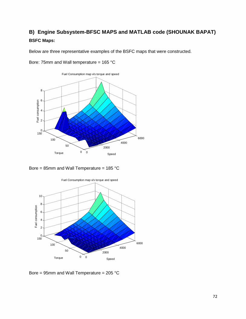
B) Engine Subsystem-BFSC MAPS and MATLAB code (SHOUNAK BAPAT) BSFC Maps:
Below are three representative examples of the BSFC maps that were constructed.
Bore: 75mm and Wall temperature = 165 °C
Bore = 85mm and Wall Temperature = 185 °C
Bore = 95mm and Wall Temperature = 205 °C
02000
40006000
0
50
100
1500
2
4
6
8
Speed
Fuel Consumption map v/s torque and speed
Torque
Fuel
con
sum
ptio
n
02000
40006000
0
50
100
1500
2
4
6
8
10
Speed
Fuel Consumption map v/s torque and speed
Torque
Fuel
con
sum
ptio
n
72

MATLAB Code for Subsystem Optimization:
Fmincon Code:
%% ME 555 Design Optimization Course Project % Engine Subsystem - Shounak Bapat %-------------------------------------------------------------------------- %Code using fmincon to optimize the bsfc of an engine %-------------------------------------------------------------------------- %clc; clear all; %Initial Guess x0 = [80; 74; 21; 10]; % x1 = bore(mm); x2 = stroke(mm); x3 = compression ratio; x4 = injection timing (CAD BTDC); LB = [75 60 17 -10]'; %Lower Bound UB = [100 110 22 25]'; %Upper Bound opts = optimset('Algorithm', 'sqp', 'DiffMinChange',0.02) [t,feval,eflag,output] = cheap_optim(x0, LB,UB, opts)
Cheap_Optim Code:
function [x,f,eflag, output] = cheap_optim(x0,LB,UB, opts) if nargin == 1 % No options supplied opts = []; end xLast = []; % Last place model was called myf = []; % Use for objective at xLast myc = []; % Use for nonlinear inequality constraint myceq = []; % Use for nonlinear equality constraint
02000
40006000
0
50
100
1500
5
10
15
Speed
Fuel Consumption map v/s torque and speed
Torque
Fuel
con
sum
ptio
n
73

fun =@objfun; % the objective function cfun = @constr; % the constraint function [x,f,eflag, output] = fmincon(fun,x0,[],[],[],[],LB,UB,cfun,opts); function f = objfun(x) if ~isequal(x,xLast) [myf, myc] = engine_model(x); xLast = x end f = myf; end function [c,ceq] = constr(x) if ~isequal(x,xLast) [myf,myc] = engine_model(x); xLast = x end c = myc; ceq = []; end end
AMESIM_Code:
%% Engine Subsystem Objective function function [f,c] = engine_model(x) %% Unpack the AMESim model file [sts, res]=system('AMELoad N:\windat.V2\Desktop\ME_555_Design_Optimization\Engine_Subsystem\ME555_Eng_SS_DID4C'); if sts~=0 disp('Loading error!') disp(res) end %% Set paramters bore = x(1) % in mm stroke = x(2) % in mm ratio = x(3) % compression ratio InjTiming = x(4) %CAD BTDC %% Assign simulation parameters ameputgpar('ME555_Eng_SS_DID4C', 'bore', bore); ameputgpar('ME555_Eng_SS_DID4C', 'stroke', stroke); ameputgpar('ME555_Eng_SS_DID4C', 'ratio', ratio); ameputgpar('ME555_Eng_SS_DID4C', 'InjTiming', InjTiming);
74

%% Run simulation [Results, VarNames]= amerun('ME555_Eng_SS_DID4C', 0, 1); %% Extract results bmep = 100*max(amegetvar(Results,VarNames,'ENGFMEP03_1 brake mean effective pressure at port 4 [bar]'));% value in kPa fuel_injected = max(amegetvar(Results,VarNames,'ENGCHMELA12_4 mass of fuel injected [mg]')) %mass in miligram injected per cylinder [? confirm once] rpm = max(amegetvar(Results,VarNames,'ENGCHMELA12_4 engine speed [rev/min]'));%speed in rev/min Vcyl = 1000 * (pi*(1/4)*((bore*0.001)^2 )* (stroke*0.001));% volume of a cylinder in dm^3 power = bmep*(4*Vcyl)*(rpm/60)/(1000*2) % in kilowatt inj_duration = 120/rpm; mass_inj_rate = ((4*fuel_injected)/inj_duration)*0.001 %in gram per second bsfc = (mass_inj_rate/power)*1000 % in micro-gram/Joule f = bsfc; c = [60 - power; x(2) - 1.2*x(1); 0.9*x(1) - x(2);7 - 2*(rpm/60)*0.001*stroke; 2*(rpm/60)*0.001*stroke - 15]; MATLAB Code for generating fuel consumption maps:
Outer Loop: close all; clear all; clc; bore=[75,80,85,90,95]; temp = [165,175,185,195,205]; %lower limit decided by maximum drop in temperature radiator can produce and upper limit decided by the average of T50 and T90 standard diesel %speed = linspace(600,6000,10); speed = [600,1500,1700,2000,2300,2700,3000, 3700,4600,6000] injec = [0.0004 0.0008,0.0010,0.0012,0.0014,0.0016,0.0017,0.0018,0.0020,0.0022,0.0024]; %Bore loop for i = 4:length(bore) %temperature loop for j = 5:length(temp) filename = ['./ExFiles/Map_',num2str(i),'_',num2str(j),'.mat']; %Map = zeros(length(injec),length(speed)); Map = zeros(11,length(speed)); tic %Speed loop for w = 1:length(speed)
75
Torque = zeros(1,length(injec)); %array to store torque total_mass = zeros(1,length(injec));%array to store mass %Injection timing loop for t = 1:length(injec) %Get the torque and mass injected data [tor,mass] = model(bore(i),temp(j),speed(w),injec(t)); Torque(t) = tor; total_mass(t) = mass; end Torque total_mass A = [Torque; total_mass]' A = sortrows(A) Torque = A(:,1); total_mass = A(:,2) %Data analysis of the torque and mass arrays f = fit(Torque,total_mass,'linearinterp'); %f = fit(Torque,total_mass,'poly2'); plot(Torque, f(Torque)) torque_set = linspace(0,130,11) %calculate new total mass new_tot_mass = f(torque_set) Map(:,w) = new_tot_mass; speed(w) end save(filename, 'Map'); toc end end Calling AMESIM: %% My engine Model for generating Fuel Maps % Stroke, CR and Inj Timing is maintained at the optimum value obtained % from subsystem optimization function [Torque, mass] = model(bore,T, speed, Tinj) %% Unpack the AMESim model file % EV_metamodel is the name of my AMESim model file. [sts, res]=system('AMELoad N:\windat.V2\Desktop\ME_555_Design_Optimization\Engine_Subsystem\making_maps\ME555_Eng_SS_DID4C'); if sts~=0 disp('Loading error!') disp(res) end
76

%% Set paramters % Design variables: Temperatures, bore, speed and injection % duration. Set the optimized values for stroke, CR and % injection timing %T is to be given in degree celsius Twall3 = T + 273; %temperature of cylinder wall in K Twall2 = Twall3 + 20; %temperature of cylinder head in K Twall1 = Twall3 - 10;% in K the piston temperature %from subsystm optimization: stroke = 80;% in mm ratio = 22; % compression ratio InjTiming = 13.8;%CAD BTDC % Tinj is injection duration in seconds. It is given % directly by the parent function %% Assign simulation parameters % ameputgpar is the function allows you to edit the value of a global parameter %Assign Optimized parameters ameputgpar('ME555_Eng_SS_DID4C', 'stroke', stroke); % assign stroke value ameputgpar('ME555_Eng_SS_DID4C', 'InjTiming', InjTiming);%assign injection timing ameputgpar('ME555_Eng_SS_DID4C', 'ratio', ratio);% assign compression ratio %Assign bore and injection duration ameputgpar('ME555_Eng_SS_DID4C', 'bore', bore); % assign bore value ameputgpar('ME555_Eng_SS_DID4C', 'Tinj', Tinj); % assign injection duration %Assign wall temperatures ameputgpar('ME555_Eng_SS_DID4C', 'Twall1', Twall1); ameputgpar('ME555_Eng_SS_DID4C', 'Twall2', Twall2); ameputgpar('ME555_Eng_SS_DID4C', 'Twall3', Twall3); %Assign Speed ameputgpar('ME555_Eng_SS_DID4C', 'RPM', speed); %% Run simulation % amerun is the function that runs the simulation. % 0 is the simulation start time, 1 is the final time [Results, VarNames]= amerun('ME555_Eng_SS_DID4C', 0, 1); %% Extract results % amegetvar is the function that allow you to get values from blocks. % Run up to this point and check VarNames from workspace to see what variables you have.
77

% time [s] is the name of the variable that AMESim saves. You can see it in VarNames bmep = 100*max(amegetvar(Results,VarNames,'ENGFMEP03_1 brake mean effective pressure at port 4 [bar]'));% value in kPa fuel_injected = 4*(max(amegetvar(Results,VarNames,'ENGCHMELA12_4 mass of fuel injected [mg]'))) %mass in miligram injected per cylinder [? confirm once] rpm = max(amegetvar(Results,VarNames,'ENGCHMELA12_4 engine speed [rev/min]'));%speed in rev/min Vcyl = 1000 * (pi*(1/4)*((bore*0.001)^2 )* (stroke*0.001));% volume of a cylinder in dm^3 power = bmep*(4*Vcyl)*(rpm/60)/(1000*2) % in kilowatt %inj_duration = 120/rpm; %mass_inj_rate = ((fuel_injected)/inj_duration)*0.001 %in gram per second %bsfc = (mass_inj_rate/power)*1000 % in micro-gram/Joule omega = rpm*2*pi/60 Torque = (1000*power)/omega; %to convert power from kilowatt to watt, multiplying by 1000 mass = fuel_injected;
C) MATLAB Code – Electrical Subsystem (Pradeep Kodali) D) % ------------------------------------------------- E) Objective function Code F) %----------------------------------------------------------------- G) function f = obj(x) H) x1 = x(1) I) x2 = x(2) J) x3 = x(3) K) x4 = x(4) L) M) % put variables N) Ti = 1199; O) ameputgpar('01_ElectricVehicle_powertrain', 'p', x1); P) ameputgpar('01_ElectricVehicle_powertrain', 'Ls', x2); Q) ameputp('01_ElectricVehicle_powertrain', 'EMDBATF05 instance 1 number of
cells in series in one branch', x3); R) ameputgpar('01_ElectricVehicle_powertrain', 'Phif', x4); S) T) % get variables U) [Results, VarNames]= amerun('01_ElectricVehicle_powertrain', 0, Ti); V) Motor_Power = amegetvar(Results,VarNames,'PTR10_1 power [W]'); W) Batt_Volt = amegetvar(Results,VarNames,'EMDBATF05_1 open circuit voltage
[V]'); X) Batt_Curr = amegetvar(Results,VarNames,'EMDBATF05_1 output current [A]'); Y) t = amegetvar(Results,VarNames,'time [s]'); Z) eff = trapz(t,Motor_Power)/trapz(t,(Batt_Volt.*Batt_Curr))
78

AA) BB) %eff = Batt_Volt.*Batt_Curr CC) f =-eff; DD) end EE) ------------------------------------------------------------------- FF) Non linear constraints Code GG) ------------------------------------------------------------------- HH) function [g,h] = NONLCON(x) II) %non linear constraints JJ) KK) x1 = x(1); LL) x2 = x(2); MM) x3 = x(3); NN) x4 = x(4); OO) PP) Vcell = 6; % V QQ) Ti = 1199; RR) %Put variables------------------- SS) ameputgpar('01_ElectricVehicle_powertrain', 'p', x1) TT) ameputgpar('01_ElectricVehicle_powertrain', 'Ls', x2); UU) ameputp('01_ElectricVehicle_powertrain', 'EMDBATF05 instance 1 number
of cells in series in one branch', x3); VV) ameputgpar('01_ElectricVehicle_powertrain', 'Phif', x4); WW) XX) [Results, VarNames]= amerun('01_ElectricVehicle_powertrain', 0, Ti); YY) %Get Variables------------------------ ZZ) Voc = amegetvar(Results,VarNames,'EMDBATF05_1 open circuit voltage
[V]'); AAA) V = amegetvar(Results,VarNames,'EMDBATF05_1 open circuit voltage [V]'); BBB) I = amegetvar(Results,VarNames,'EMDBATF05_1 output current [A]'); CCC) R = amegetvar(Results,VarNames,'EMDBATF05_1 internal resistance
[Ohm]'); DDD) Power_Motor = amegetvar(Results,VarNames,'PTR10_2 power [W]'); EEE) Motor_Speed = amegetvar(Results,VarNames,'PTR10_2 angular velocity at
port 1 [rev/min]'); FFF) GGG) g = [ HHH) max(0.5*(Voc - sqrt(Voc.^2 - 4.*R.*V.*I)))-x3*Vcell; III) max(abs(Power_Motor)) - 60000; JJJ) 26000-max(abs(Power_Motor)); KKK) max(abs(Motor_Speed)) - 12000; LLL) ]; MMM) h = []; NNN) end OOO) %------------------------------------------------------------------- PPP) Main function code QQQ) %------------------------------------------------------------------- %% ME 555 Design Optimization Battery Subsystem %Pradeep Kodali clear all
79

close all clc %------------------------------------------------------------ % Use your own path % EV_metamodel is the name of my AMESim model file. [sts, res]=system('AMELoad N:\windat.V2\Documents\Downloads\DES_OPT\01_ElectricVehicle_powertrain'); if sts~=0 disp('Loading error!') disp(res) end diary; %------------------------------------------------------------- % options =optimset('Display','iter','LargeScale','off'); A=[];b=[];Aeq=[];beq=[]; LB=[1;0.0015;50;0.1]; UB=[5;0.006;150;0.5]; vfun=@(x)obj(x); % Set constraint function nonlcon=@(x)NONLCON(x); populations=50; %set population size generations=10; %set number of generations des_var =4; intcon =[1,3]; % initial guess will be 100 x 4 matrix %ini=rand(100,4); rng(1); ini(:,1) = randi([1 5],50,1); ini(:,3) = randi([50 150],50,1); ini(:,2) = 0.0015 + (0.006-0.0015)*rand(50,1); ini(:,4) = 0.1 + (0.5-0.1)*rand(50,1); % ini_values = [2,0.002,114,0.2]; % ini = repmat(ini_values,100,1); %-------------------------------------------------------------------- % @gaplotbestfun will show you a convergence plot. Based on this, tune population size and number of generations options = gaoptimset('InitialPopulation',ini,'PopulationSize',populations,'Generations',generations,'PlotFcns',@gaplotbestfun); [xopt,fval,exitflag,output] = ga(vfun,des_var,A,b,Aeq,beq,LB,UB,nonlcon,intcon,options); %[xopt,fval,exitflag,ouput] = ga(@obj,des_var,A,b,Aeq,beq,LB,UB,[],x0,options); [sts, res]=system('AMESave N:\windat.V2\Documents\Downloads\DES_OPT\01_ElectricVehicle_powertrain'); %------------------------------------------------------------------- Neural network meta function for f %-------------------------------------------------------------------
80

function [Y,Xf,Af] = f_obj(X,~,~) %MYNEURALNETWORKFUNCTION neural network simulation function. % % Generated by Neural Network Toolbox function genFunction, 14-Apr-2015 21:09:56. % % [Y] = myNeuralNetworkFunction(X,~,~) takes these arguments: % % X = 1xTS cell, 1 inputs over TS timsteps % Each X{1,ts} = 4xQ matrix, input #1 at timestep ts. % % and returns: % Y = 1xTS cell of 1 outputs over TS timesteps. % Each Y{1,ts} = 1xQ matrix, output #1 at timestep ts. % % where Q is number of samples (or series) and TS is the number of timesteps. %#ok<*RPMT0> % ===== NEURAL NETWORK CONSTANTS ===== % Input 1 x1_step1_xoffset = [1;50;0.002;0.15]; x1_step1_gain = [0.5;0.02;500;10]; x1_step1_ymin = -1; % Layer 1 b1 = [-0.45656982664811491;1.0630832215016865;0.60583829063205197;0.29794457931781065;3.0499664158104611;-1.8448314678291473]; IW1_1 = [-1.0296512591183156 0.35846075064946981 0.22565450677956578 -0.29243338711112371;0.29764057315443554 0.36764936978931256 0.067269573276008604 -0.016665733067330754;0.52039511712763442 -0.030212349365546096 0.025441613588724439 -0.5474781660667799;1.0164163185647175 -0.19967659131284521 -0.15004715022074799 0.021847133221980678;-0.84425729046823716 0.47693078686662793 1.568693840290009 -0.7967721730508488;-1.3220622236851736 0.21029908014347576 -0.025536064718731179 -0.49938252822003276]; % Layer 2 b2 = 3.3702753514105139; LW2_1 = [1.4127082988405084 -1.9893914688796244 -0.64243999950488928 1.8012943378262791 -0.71335806684407266 1.5578873519977672]; % Output 1 y1_step1_ymin = -1; y1_step1_gain = 5.10836402396209; y1_step1_xoffset = -0.813930037344394; % ===== SIMULATION ======== % Format Input Arguments isCellX = iscell(X); if ~isCellX, X = {X}; end;
81

% Dimensions TS = size(X,2); % timesteps if ~isempty(X) Q = size(X{1},2); % samples/series else Q = 0; end % Allocate Outputs Y = cell(1,TS); % Time loop for ts=1:TS % Input 1 Xp1 = mapminmax_apply(X{1,ts},x1_step1_gain,x1_step1_xoffset,x1_step1_ymin); % Layer 1 a1 = tansig_apply(repmat(b1,1,Q) + IW1_1*Xp1); % Layer 2 a2 = repmat(b2,1,Q) + LW2_1*a1; % Output 1 Y{1,ts} = mapminmax_reverse(a2,y1_step1_gain,y1_step1_xoffset,y1_step1_ymin); end % Final Delay States Xf = cell(1,0); Af = cell(2,0); % Format Output Arguments if ~isCellX, Y = cell2mat(Y); end end % ===== MODULE FUNCTIONS ======== % Map Minimum and Maximum Input Processing Function function y = mapminmax_apply(x,settings_gain,settings_xoffset,settings_ymin) y = bsxfun(@minus,x,settings_xoffset); y = bsxfun(@times,y,settings_gain); y = bsxfun(@plus,y,settings_ymin); end % Sigmoid Symmetric Transfer Function function a = tansig_apply(n) a = 2 ./ (1 + exp(-2*n)) - 1; end % Map Minimum and Maximum Output Reverse-Processing Function function x = mapminmax_reverse(y,settings_gain,settings_xoffset,settings_ymin)
82
x = bsxfun(@minus,y,settings_ymin); x = bsxfun(@rdivide,x,settings_gain); x = bsxfun(@plus,x,settings_xoffset); end %------------------------------------------------------------------- Neural network meta function for g speed %------------------------------------------------------------------- function [Y,Xf,Af] = g_speed(X,~,~) %MYNEURALNETWORKFUNCTION neural network simulation function. % % Generated by Neural Network Toolbox function genFunction, 14-Apr-2015 23:13:47. % % [Y] = myNeuralNetworkFunction(X,~,~) takes these arguments: % % X = 1xTS cell, 1 inputs over TS timsteps % Each X{1,ts} = 4xQ matrix, input #1 at timestep ts. % % and returns: % Y = 1xTS cell of 1 outputs over TS timesteps. % Each Y{1,ts} = 1xQ matrix, output #1 at timestep ts. % % where Q is number of samples (or series) and TS is the number of timesteps. %#ok<*RPMT0> % ===== NEURAL NETWORK CONSTANTS ===== % Input 1 x1_step1_xoffset = [1;50;0.002;0.15]; x1_step1_gain = [0.5;0.02;500;10]; x1_step1_ymin = -1; % Layer 1 b1 = [-0.39718929665494851;0.087890619156085939;1.4408656455971101;1.9634377542621735;1.4512564350888224;-1.9198872084252443;0.26006031320005085;-0.22562847969330335;1.089115324465914;-0.040839963032721416]; IW1_1 = [-0.28345773335270064 0.032311266704569949 0.33690273716288505 -0.069729734074586117;-0.020919475347270892 -0.91417364871456608 0.12273869338901218 -0.78041338860593124;0.0052627916313738735 1.2211533449504144 -0.32458649799579475 -0.16883830065857561;0.018147505349268029 -2.0065019725557822 2.6683979536694209 -2.1076663222394809;0.054958980096212175 0.36204359476626563 -0.21943414248583962 1.1285217222228727;-0.012473542023031041 2.3610808376352219 -2.9568034785213499 2.1361447629796637;-0.0013004913627570201 0.92699325004217592 -0.68107076740048078 0.51228392054262539;-0.36427584283971381 0.074709016448828644 0.26963471210918116 -0.2049358858719206;0.16130060563999216 -0.054210442153161384 0.2223208270033869 0.37702356492425521;0.0091624053498097421 0.97566859860169153 -0.31898484116756293 0.60768500260054481]; % Layer 2 b2 = 0.48416888824251142;
83
LW2_1 = [1.1863272443025858 -0.73955563096174703 0.52620637060318975 0.39655978820040849 0.50037587744012546 0.44476575391987483 1.0426524126838852 -0.98105522559355829 -0.98044856212646458 -1.349689532151241]; % Output 1 y1_step1_ymin = -1; y1_step1_gain = 0.000637064162171028; y1_step1_xoffset = -9686.36817635052; % ===== SIMULATION ======== % Format Input Arguments isCellX = iscell(X); if ~isCellX, X = {X}; end; % Dimensions TS = size(X,2); % timesteps if ~isempty(X) Q = size(X{1},2); % samples/series else Q = 0; end % Allocate Outputs Y = cell(1,TS); % Time loop for ts=1:TS % Input 1 Xp1 = mapminmax_apply(X{1,ts},x1_step1_gain,x1_step1_xoffset,x1_step1_ymin); % Layer 1 a1 = tansig_apply(repmat(b1,1,Q) + IW1_1*Xp1); % Layer 2 a2 = repmat(b2,1,Q) + LW2_1*a1; % Output 1 Y{1,ts} = mapminmax_reverse(a2,y1_step1_gain,y1_step1_xoffset,y1_step1_ymin); end % Final Delay States Xf = cell(1,0); Af = cell(2,0); % Format Output Arguments if ~isCellX, Y = cell2mat(Y); end end % ===== MODULE FUNCTIONS ========
84
% Map Minimum and Maximum Input Processing Function function y = mapminmax_apply(x,settings_gain,settings_xoffset,settings_ymin) y = bsxfun(@minus,x,settings_xoffset); y = bsxfun(@times,y,settings_gain); y = bsxfun(@plus,y,settings_ymin); end % Sigmoid Symmetric Transfer Function function a = tansig_apply(n) a = 2 ./ (1 + exp(-2*n)) - 1; end % Map Minimum and Maximum Output Reverse-Processing Function function x = mapminmax_reverse(y,settings_gain,settings_xoffset,settings_ymin) x = bsxfun(@minus,y,settings_ymin); x = bsxfun(@rdivide,x,settings_gain); x = bsxfun(@plus,x,settings_xoffset); end %------------------------------------------------------------------- Neural network meta function for g power max %------------------------------------------------------------------- function [Y,Xf,Af] = g_power_max(X,~,~) %MYNEURALNETWORKFUNCTION neural network simulation function. % % Generated by Neural Network Toolbox function genFunction, 14-Apr-2015 23:07:02. % % [Y] = myNeuralNetworkFunction(X,~,~) takes these arguments: % % X = 1xTS cell, 1 inputs over TS timsteps % Each X{1,ts} = 4xQ matrix, input #1 at timestep ts. % % and returns: % Y = 1xTS cell of 1 outputs over TS timesteps. % Each Y{1,ts} = 1xQ matrix, output #1 at timestep ts. % % where Q is number of samples (or series) and TS is the number of timesteps. %#ok<*RPMT0> % ===== NEURAL NETWORK CONSTANTS ===== % Input 1 x1_step1_xoffset = [1;50;0.002;0.15]; x1_step1_gain = [0.5;0.02;500;10]; x1_step1_ymin = -1; % Layer 1 b1 = [-0.20770968683623722;-0.061787199466784973;3.6964731943243518;0.74270786820051182;-2.7903294737048174;1.2300683757572952;-1.744743928962063;0.8329705165310809;1.0404780760858297;2.7803050193798828];
85
IW1_1 = [-0.08553970426878986 1.0331105611052873 -0.45013155333612909 0.22098971820071947;0.0065689405839856763 0.26173612930503204 0.89239823017306064 -0.048973961600320519;1.1729165935620218 -0.73989913817712061 0.97830713759477561 0.22627181797417734;-0.016343398453510859 0.95255159873783379 0.25956333547287685 0.0038159992139904131;-1.0188457003875833 0.83824950169028312 -0.78094149787898703 -0.22103090748695609;-0.12644401914261369 -0.50682264591752046 0.96055289742923522 -0.62583535238924448;0.07846235575531256 0.43443464481216465 -1.1570432542660685 0.98418548520075055;-0.037477184513176748 -0.42867342337457004 0.0339773997305199 0.17945570824030704;-0.030312045181915964 1.3526776806469949 0.044503703721885286 0.064417502161218526;0.1816620663570945 -1.5804855092455412 2.8223584532595578 -1.3305207012882032]; % Layer 2 b2 = -1.8238621129449175; LW2_1 = [0.55816676545948607 0.21235298900170185 2.3757886726430275 -0.99992408825277768 0.87682191933423748 -1.2930713227723014 -0.92350532928102924 0.84300732058681682 0.88464161493801663 -0.22516315479560911]; % Output 1 y1_step1_ymin = -1; y1_step1_gain = 5.11494078973706e-05; y1_step1_xoffset = -56220.257566847; % ===== SIMULATION ======== % Format Input Arguments isCellX = iscell(X); if ~isCellX, X = {X}; end; % Dimensions TS = size(X,2); % timesteps if ~isempty(X) Q = size(X{1},2); % samples/series else Q = 0; end % Allocate Outputs Y = cell(1,TS); % Time loop for ts=1:TS % Input 1 Xp1 = mapminmax_apply(X{1,ts},x1_step1_gain,x1_step1_xoffset,x1_step1_ymin); % Layer 1 a1 = tansig_apply(repmat(b1,1,Q) + IW1_1*Xp1); % Layer 2
86

a2 = repmat(b2,1,Q) + LW2_1*a1; % Output 1 Y{1,ts} = mapminmax_reverse(a2,y1_step1_gain,y1_step1_xoffset,y1_step1_ymin); end % Final Delay States Xf = cell(1,0); Af = cell(2,0); % Format Output Arguments if ~isCellX, Y = cell2mat(Y); end end % ===== MODULE FUNCTIONS ======== % Map Minimum and Maximum Input Processing Function function y = mapminmax_apply(x,settings_gain,settings_xoffset,settings_ymin) y = bsxfun(@minus,x,settings_xoffset); y = bsxfun(@times,y,settings_gain); y = bsxfun(@plus,y,settings_ymin); end % Sigmoid Symmetric Transfer Function function a = tansig_apply(n) a = 2 ./ (1 + exp(-2*n)) - 1; end % Map Minimum and Maximum Output Reverse-Processing Function function x = mapminmax_reverse(y,settings_gain,settings_xoffset,settings_ymin) x = bsxfun(@minus,y,settings_ymin); x = bsxfun(@rdivide,x,settings_gain); x = bsxfun(@plus,x,settings_xoffset); end %------------------------------------------------------------------- Neural network meta function for g power min %------------------------------------------------------------------- function [Y,Xf,Af] = g_power_min(X,~,~) %MYNEURALNETWORKFUNCTION neural network simulation function. % % Generated by Neural Network Toolbox function genFunction, 14-Apr-2015 23:11:23. % % [Y] = myNeuralNetworkFunction(X,~,~) takes these arguments: % % X = 1xTS cell, 1 inputs over TS timsteps % Each X{1,ts} = 4xQ matrix, input #1 at timestep ts. % % and returns: % Y = 1xTS cell of 1 outputs over TS timesteps. % Each Y{1,ts} = 1xQ matrix, output #1 at timestep ts. %
87

% where Q is number of samples (or series) and TS is the number of timesteps. %#ok<*RPMT0> % ===== NEURAL NETWORK CONSTANTS ===== % Input 1 x1_step1_xoffset = [1;50;0.002;0.15]; x1_step1_gain = [0.5;0.02;500;10]; x1_step1_ymin = -1; % Layer 1 b1 = [-1.0025412250829158;-0.20831623137998739;2.3292600181725418;-0.67481349040261707;0.50859022570692691;0.51122559053756111;-0.32283971721613863;-0.28633586774415987;0.55524473136508501;0.8469905818021799]; IW1_1 = [-0.15282379226858703 0.54902716666790363 -0.9442730527328822 0.78690433046224384;0.026905885953630887 0.16098681210156818 -0.69839107741684769 0.21240303561103782;0.061524442022090849 -1.3602197667443883 2.1517355451428339 -1.1697201008188853;0.050669535183569585 -0.29151840830039849 -0.14345497329154761 0.35313371721643766;0.80950920779608981 -0.27101842052450836 0.77765744215160015 -0.037422622729810555;-0.017490936586495188 -0.95282952891570249 0.33805961671273604 -0.16334063548773989;0.0015545967886123439 0.75612600638341976 -0.51913341768392163 0.22361614017769582;0.078610046487505331 -0.060260422308445243 -0.43733818753040943 0.30993818848934473;0.10299964860176426 -0.2720104461571613 -0.29927799496110397 -0.1166816290913275;0.13799325918611399 -0.70120856350869387 1.2834473095855234 -0.99689636793535608]; % Layer 2 b2 = 0.064222069601250778; LW2_1 = [1.0622820876307635 1.0770880802228704 0.52000828512199782 1.0916543048334524 0.11453967036757944 -1.2014777810573911 -1.8933271193793237 -1.9180656701980154 0.68717113831751664 0.57644533881241944]; % Output 1 y1_step1_ymin = -1; y1_step1_gain = 5.11494078973706e-05; y1_step1_xoffset = -16880.8793224192; % ===== SIMULATION ======== % Format Input Arguments isCellX = iscell(X); if ~isCellX, X = {X}; end; % Dimensions TS = size(X,2); % timesteps if ~isempty(X) Q = size(X{1},2); % samples/series else Q = 0;
88

end % Allocate Outputs Y = cell(1,TS); % Time loop for ts=1:TS % Input 1 Xp1 = mapminmax_apply(X{1,ts},x1_step1_gain,x1_step1_xoffset,x1_step1_ymin); % Layer 1 a1 = tansig_apply(repmat(b1,1,Q) + IW1_1*Xp1); % Layer 2 a2 = repmat(b2,1,Q) + LW2_1*a1; % Output 1 Y{1,ts} = mapminmax_reverse(a2,y1_step1_gain,y1_step1_xoffset,y1_step1_ymin); end % Final Delay States Xf = cell(1,0); Af = cell(2,0); % Format Output Arguments if ~isCellX, Y = cell2mat(Y); end end % ===== MODULE FUNCTIONS ======== % Map Minimum and Maximum Input Processing Function function y = mapminmax_apply(x,settings_gain,settings_xoffset,settings_ymin) y = bsxfun(@minus,x,settings_xoffset); y = bsxfun(@times,y,settings_gain); y = bsxfun(@plus,y,settings_ymin); end % Sigmoid Symmetric Transfer Function function a = tansig_apply(n) a = 2 ./ (1 + exp(-2*n)) - 1; end % Map Minimum and Maximum Output Reverse-Processing Function function x = mapminmax_reverse(y,settings_gain,settings_xoffset,settings_ymin) x = bsxfun(@minus,y,settings_ymin); x = bsxfun(@rdivide,x,settings_gain); x = bsxfun(@plus,x,settings_xoffset); end %-------------------------------------------------------------------
89

Neural network meta function for g volt max %------------------------------------------------------------------- function [Y,Xf,Af] = g_voltage(X,~,~) %MYNEURALNETWORKFUNCTION neural network simulation function. % % Generated by Neural Network Toolbox function genFunction, 14-Apr-2015 22:07:58. % % [Y] = myNeuralNetworkFunction(X,~,~) takes these arguments: % % X = 1xTS cell, 1 inputs over TS timsteps % Each X{1,ts} = 4xQ matrix, input #1 at timestep ts. % % and returns: % Y = 1xTS cell of 1 outputs over TS timesteps. % Each Y{1,ts} = 1xQ matrix, output #1 at timestep ts. % % where Q is number of samples (or series) and TS is the number of timesteps. %#ok<*RPMT0> % ===== NEURAL NETWORK CONSTANTS ===== % Input 1 x1_step1_xoffset = [1;50;0.002;0.15]; x1_step1_gain = [0.5;0.02;500;10]; x1_step1_ymin = -1; % Layer 1 b1 = [-0.15525095401584785;0.083859853463873119;1.3825833449142824;-0.64158424285469051;0.02916403726839685;0.51629222733090874;-0.10756667348626293;0.5223470572856459;0.19326930828456759;-1.2281020721071085]; IW1_1 = [0.52133244636470499 0.1874363798513147 0.085643294753188326 0.2838511436856414;-0.06822838294248873 0.19659459210007571 0.03067335418669449 0.23643015337074741;0.009179489928275119 -0.65466574376554754 0.80068771028742758 0.44928307873850232;0.020267413360626058 -0.66157086800209586 0.35685044586861164 -0.23114261901434896;0.024760446939503581 -0.16327491949831563 -0.17348458060397015 -0.22225713188790974;0.007379234327457059 0.98829581222260388 0.22619499130576015 -0.1582139049681732;0.41879206234285954 0.18519130474555151 0.096937664213596259 0.25783563948941357;0.00040339544820285804 0.87136185824657086 0.06327827715293266 -0.044382185911144928;-0.059584915502767122 0.24799818889839609 -0.12297943991083449 0.26003397303861414;-0.0024470655593651653 1.6641931923595574 -0.0018370086156256533 0.00026473169698248592]; % Layer 2 b2 = 0.21948086561590049; LW2_1 = [0.20046349588740589 -0.65079382278286013 0.0090185698993558248 0.16381293354812185 -0.32127129993199233 0.21878375901738753 -0.28223458621252207 -1.2792961179240629 0.44988714011393038 -0.41889579916024983];
90

% Output 1 y1_step1_ymin = -1; y1_step1_gain = 0.00220456853314718; y1_step1_xoffset = -1344.93557324929; % ===== SIMULATION ======== % Format Input Arguments isCellX = iscell(X); if ~isCellX, X = {X}; end; % Dimensions TS = size(X,2); % timesteps if ~isempty(X) Q = size(X{1},2); % samples/series else Q = 0; end % Allocate Outputs Y = cell(1,TS); % Time loop for ts=1:TS % Input 1 Xp1 = mapminmax_apply(X{1,ts},x1_step1_gain,x1_step1_xoffset,x1_step1_ymin); % Layer 1 a1 = tansig_apply(repmat(b1,1,Q) + IW1_1*Xp1); % Layer 2 a2 = repmat(b2,1,Q) + LW2_1*a1; % Output 1 Y{1,ts} = mapminmax_reverse(a2,y1_step1_gain,y1_step1_xoffset,y1_step1_ymin); end % Final Delay States Xf = cell(1,0); Af = cell(2,0); % Format Output Arguments if ~isCellX, Y = cell2mat(Y); end end % ===== MODULE FUNCTIONS ======== % Map Minimum and Maximum Input Processing Function function y = mapminmax_apply(x,settings_gain,settings_xoffset,settings_ymin) y = bsxfun(@minus,x,settings_xoffset);
91

y = bsxfun(@times,y,settings_gain); y = bsxfun(@plus,y,settings_ymin); end % Sigmoid Symmetric Transfer Function function a = tansig_apply(n) a = 2 ./ (1 + exp(-2*n)) - 1; end % Map Minimum and Maximum Output Reverse-Processing Function function x = mapminmax_reverse(y,settings_gain,settings_xoffset,settings_ymin) x = bsxfun(@minus,y,settings_ymin); x = bsxfun(@rdivide,x,settings_gain); x = bsxfun(@plus,x,settings_xoffset); end %------------------------------------------------------------------- Nonlcon for fmincon %------------------------------------------------------------------- function [g,h] = NONLCON_fmincon(x) %non linear constraints g=[g_voltage(x); g_power_max(x); g_power_min(x); g_speed(x)]; h=[]; %------------------------------------------------------------------- Nonlcon for fmincon %------------------------------------------------------------------- %% ME 555 Design Optimization Battery Subsystem %Pradeep Kodali clear all close all clc %------------------------------------------------------------ % Use your own path % EV_metamodel is the name of my AMESim model file. % [sts, res]=system('AMELoad N:\windat.V2\Documents\Downloads\DES_OPT\01_ElectricVehicle_powertrain'); % if sts~=0 % disp('Loading error!') % disp(res) % end diary; %------------------------------------------------------------- % options =optimset('Display','iter','LargeScale','off'); A=[];b=[];Aeq=[];beq=[]; lb=[1;50;0.0015;0.1]; ub=[5;150;0.006;0.5]; % vfun=@(x)f_obj(x); % % Set constraint function % nonlcon=@(x)NONLCON_fmincon(x); % populations=50; %set population size
92

% generations=10; %set number of generations % des_var =4; % intcon =[1,3]; % initial guess will be 100 x 4 matrix %ini=rand(100,4); % rng(1); % ini(:,1) = randi([1 5],50,1); % ini(:,3) = randi([50 150],50,1); % ini(:,2) = 0.0015 + (0.006-0.0015)*rand(50,1); % ini(:,4) = 0.1 + (0.5-0.1)*rand(50,1); ini_values = [1,50,0.002,0.2]'; % ini = repmat(ini_values,100,1); %-------------------------------------------------------------------- % @gaplotbestfun will show you a convergence plot. Based on this, tune population size and number of generations %options = gaoptimset('InitialPopulation',ini,'PopulationSize',populations,'Generations',generations,'PlotFcns',@gaplotbestfun); %options =optimset('Display','iter','LargeScale','off'); options = optimoptions(@fmincon,'Algorithm','sqp','Display','off'); [xopt,fval,exitflag,ouput] = fmincon('f_obj',ini_values,A,b,Aeq,beq,lb,ub,'NONLCON_fmincon',options) %[xopt,fval,exitflag,ouput] = ga(@obj,des_var,A,b,Aeq,beq,LB,UB,[],x0,options); [sts, res]=system('AMESave N:\windat.V2\Documents\Downloads\DES_OPT\01_ElectricVehicle_powertrain'); %------------------------------------------------------------------- Code for map generation %------------------------------------------------------------------- %% ME 555 Design Optimization Battery Subsystem %Pradeep Kodali clear all close all clc %------------------------------------------------------------ % Use your own path % EV_metamodel is the name of my AMESim model file. [sts, res]=system('AMELoad N:\windat.V2\Documents\Downloads\DES_OPT\01_ElectricVehicle_maps'); if sts~=0 disp('Loading error!') disp(res) end %diary; %------------------------------------------------------------- % cd(matlabroot); % cd('N:\windat.V2\Documents\Downloads\DES_OPT'); % ds = dataset('XLSFile','map_var.xlsx'); i=1;j=1;k=1; %speed_trq = zeros(25,25); eff_val = NaN*zeros(12,10,5);
93

speed_val_op = NaN*zeros(12,10,5); trq_val_op = NaN*zeros(12,10,5); trq_val_ip = NaN*zeros(12,10,5); phi =[0.2834,0.35,0.4,0.45,0.5]; speed = [-500,-1000,-1500,-2000,-2500,-3000,-3500,-4000,-4500,-5000,-5500,-6000]/5; torque = [305,275,250,225,200,175,150,125,100,50]; Ti = 350; for i=1:length(phi) ameputgpar('01_ElectricVehicle_maps', 'Phif', phi(i)); for j=1:length(speed) ameputgpar('01_ElectricVehicle_maps', 'SpeedIn', speed(j)); for k = 1:length(torque) torque(k) try ameputgpar('01_ElectricVehicle_maps', 'TorqueIn', torque(k)); [Results, VarNames]= amerun('01_ElectricVehicle_maps', 0, Ti); Mot_speed = amegetvar(Results,VarNames,'MECRSS0B_1 angular velocity at port 3 [rev/min]'); Mot_Torque = amegetvar(Results,VarNames,'MECRSS0B_1 torque at port 3 [Nm]'); Input_torque = amegetvar(Results,VarNames,'EMDSMPEFOC01_1 torque command at port 9 [Nm]'); output_power = amegetvar(Results,VarNames,'PTR10_1 power [W]'); input_volt = amegetvar(Results,VarNames,'ESCAVINV01_1 DC potential at port 8 [V]'); input_curr = amegetvar(Results,VarNames,'ESCAVINV01_1 DC current at port 8 [A]'); eff = output_power(end)/(-input_volt(end)*input_curr(end)); eff_val(j,k,i) =eff; speed_val_op(j,k,i) = Mot_speed(end); trq_val_op(j,k,i) = Mot_Torque(end); trq_val_ip(j,k,i) = Input_torque(end); catch disp(i) disp(j) disp(k) end end end end [sts, res]=system('AMESave N:\windat.V2\Documents\Downloads\DES_OPT\01_ElectricVehicle_maps');
94

RRR) MATLAB Code – Planetary Gear system (Vijay Kumar Singla) sim_data.m
%by Vijay Kumar Singla scale=0.2; e_inertia=0.18; % (kg*m^2), rotational inertia of the engine % SPEED & TORQUE RANGES over which data is defined % (rad/s), speed range of the engine eng_map_spd=[600:200:2400, 2800:400:4000, 4800:400:6400]*2*pi/60; eng_map_fuel=0:0.05:1; eng_map_trq = [-32 -46 -61.0157 -72.0418 -88.5749 -113.05 -121.754 -133.211 -149.115 -155.8 -161.783 -179.27 -202 -226 -291 -313 -326 -329 -334 63.2274 18.3572 -6.65404 -20.8056 -35.8626 -54.5064 -66.1904 -77.923 -92.6959 -103.4 -112.11 -131.211 -150 -180 -249 -271 -271 -278 -281 162.046 112.123 73.8496 44.1625 19.4438 4.03722 -10.6267 -22.6354 -36.2766 -49.2 -62.4367 -83.1514 -104 -140.991 -204 -218 -227 -231 -236 241.396 199.546 152.977 116.651 89.3922 67.0513 49.0455 33.3358 20.1428 6.31236 -12.7637 -35.0921 -59 -87.2085 -151 -167 -173.327 -172.828 -172.329 291.911 269.978 235.086 197.766 160.047 131.786 110.02 90.8644 73.6912 60.8065 36.3067 12.9672 -5.44728 -33.4263 -90 -105.706 -111.43 -117.154 -122.878 327.075 317.388 295.385 268.212 238.284 207.273 175.003 155.504 132.594 114.731 88.9138 59.8482 38.3908 20.356 -25.6394 -37.5853 -49.5312 -61.4771 -73.423 346.42 350.631 351.7 341.8 332.089 313.374 293.784 269.418 246.786 224.05 180.873 143.932 115.613 90.2755 48.5938 30.5351 12.4764 -5.5823 -23.641 349.281 362.497 372.1 377.103 381.798 376.26 366.595 359.843 347.256 329.945 296.299 259.138 219.179 184.254 125.861 103.157 80.453 57.749 35.045 352.143 368 379.3 390.82 398.6 408.848 406.54 405.697 397.687 389.591 372.719 338.564 312.511 279.313 199.295 174.543 149.791 125.039 100.287 355.004 373 386.1 396 407.41 421.386 425.556 429.651 429.188 430.66 419 400 382.177 358.394 288.322 259.317 230.312 201.307 172.302 357.866 378 389.52 402.3 412.231 426.807 435.015 441.503 447.205 449.526 451.055 436 423.741 411.318 362.61 331.317 300.024 268.731 237.438 360.727 381.89 391.087 407.3 417.053 432.228 440.759 447.608 453.557 462.963 464.551 458 458.579 448.932 419.75 394.06 361.7 321.5 277.8 363.589 383.04 392.654 411.59 421.874 437.649 446.502 453.713 459.909 473.702 476.043 474.857 478.396 479.511 458.966 436.686 402.8 358.6 311.6 366.45 384.19 394.221 412.94 425.678 443.727 452.246 459.818 466.262 479.3 486.831 485.58 492.224 503.186 487.831 468.491 435.7 393.3 343.7 369.311 385.34 395.788 414.29 427.994 445.726 457.989 465.923 472.614 483.054 494.789 496.302 503.436 510.051 507.663 488.126 458.7 413.6 366.7 372.173 386.49 397.355 415.64 430.31 447.725 463.733 469.9 478.43 484.685 496.266 506.215 514.648 516.917 515.903 500.317 472.7 429.4 379.3 375.034 387.64 398.922 416.99 432.626 449.724 469.476 471.93 480.162 486.316 497.743 507.932 519.701 523.782 523.93 508.06 482.2 442 393.8 377.896 388.79 400.489 418.34 434.942 451.723 470.126 473.96 481.894 487.947 499.219 509.649 521.466 530.486 531.957 515.392 490.8 449.3 401.9
95

380.757 389.94 402.056 419.69 437.258 453.722 470.298 475.99 483.626 489.578 500.696 511.366 523.23 532.871 535.643 518.851 496.7 459.6 411.8 383.619 391.09 403.623 421.04 439.574 455.721 470.469 478.02 485.358 491.209 502.173 513.083 524.995 535.255 538.736 522.311 499.8 468.2 422.2 386.48 392.24 405.19 422.39 440.89 457.72 470.64 480.05 487.09 492.84 503.65 514.8 526.76 537.64 541.83 525.77 504.4 472.37 431.15 ]'*scale; % ENGINE FUEL CONSUMPTION %lookup map for calculate fuel consumption eng_consum_spd=[600:200:2400, 2800:400:4000, 4800:400:6400]*2*pi/60; eng_consum_trq=linspace(0,541.83*scale,21); % lbft2Nm=1.356; %conversion from lbft to Nm % (g/s), fuel use map indexed vertically by eng_consum_spd and horizontally by eng_consum_trq eng_consum_fuel=[0 0 0 0 0 0 0 0 0 0 0 0 0 0 0 0 0 0 0 0.46417 0.466285 0.471238 0.471786 0.456106 0.430872 0.417824 0.409022 0.406724 0.405708 0.415145 0.49 0.52 0.52 0.62 0.7 0.75 0.78 0.86 0.81312 0.824123 0.835126 0.846129 0.857132 0.868135 0.879138 0.890141 0.901144 0.912147 0.92315 1 1.04 1.09 1.3 1.34478 1.43 1.43 1.56 1.10624 1.22613 1.25124 1.27635 1.30146 1.32657 1.35168 1.37679 1.4019 1.42701 1.51 1.54 1.61 1.64 1.9 2.01717 2.13 2.19 2.34 1.32233 1.57292 1.72721 1.79727 1.80095 1.80463 1.80831 1.81199 1.81567 1.87 1.9 1.95 2.03 2.16 2.45 2.68955 2.81 2.89 3 1.47621 1.84244 2.1171 2.29343 2.41153 2.46909 2.4763 2.48351 2.49072 2.49793 2.6 2.63 2.73 2.81 3.07 3.36194 3.58 3.75 3.9 1.57054 2.08504 2.51113 2.85105 3.20303 3.44497 3.64347 3.75038 3.85181 3.8969 4 4.1 4.1 4.2 4.52 4.84474 5.07 5.23 5.44 1.59536 2.24719 2.74716 3.19286 3.68029 4.05266 4.41808 4.78327 5.07176 5.30439 5.71378 5.97113 6.18 6.38 7.16 7.48503 8 8.27 8.51 1.62018 2.39417 2.90107 3.38498 3.89021 4.4007 4.86025 5.31065 5.69407 6.09608 6.87164 7.39779 7.9138 8.53 9.86 10.2876 10.56 10.8 10.98 1.645 2.54115 3.05498 3.56526 4.01152 4.595 5.09443 5.59559 6.09357 6.64284 7.65 8.41333 9.34813 10.3 12.7 13.53 13.89 14.08 14.36 1.66982 2.655 3.20889 3.74553 4.13282 4.74286 5.29509 5.82413 6.35834 6.91098 8.22 9.06961 10.2034 11.47 15.07 16.11 16.68 17.09 17.25 1.69464 2.6695 3.3628 3.92581 4.25413 4.89071 5.48272 6.03345 6.61068 7.40008 8.85 10.02 11.4 13.24 17.28 18.58 19.2 19.41 19.54 1.71945 2.684 3.4858 4.10609 4.37543 5.03857 5.67035 6.24277 6.86302 7.83 9.37 10.56 12.1 14.26 19 20.4328 20.82 21.18 21.26 1.74427 2.6985 3.53999 4.20386 4.49674 5.18643 5.85798 6.45208 7.11536 8.09 9.81 11.08 12.83 15.22 20.19 21.6859 22.14 22.43 22.53 1.76909 2.713 3.59417 4.27585 4.61804 5.33428 6.04561 6.6614 7.36771 8.33 10.12 11.58 13.44 15.83 20.92 22.4603 23 23.42 23.55 1.79391 2.7275 3.64836 4.34784 4.73935 5.48214 6.23324 6.87072 7.62005 8.56085 10.3456 12.0776 13.9079 16.2008 21.2991 22.9554 23.47 23.89 24.04 1.81873 2.742 3.70255 4.41983 4.86066 5.63 6.42086 7.08004 7.87239 8.64868 10.4113 12.1621 14.278 16.3888 21.5731 23.2834 23.89 24.38 24.69 1.84355 2.7565 3.75674 4.49182 4.97754 5.72222 6.46953 7.18001 7.98226 8.73651 10.477 12.2466 14.367 16.575 21.8471 23.5947 24.22 24.77 25.11 1.86836 2.771 3.81092 4.56382 5.09082 5.78148 6.50512 7.23401 8.04207 8.82434 10.5427 12.331 14.456 16.7126 21.9649 23.7482 24.41 25.03 25.47
96

1.89318 2.7855 3.86511 4.63581 5.20411 5.84074 6.54071 7.288 8.10189 8.91217 10.6083 12.4155 14.545 16.8503 22.0615 23.9016 24.59 25.29 25.71 1.918 2.8 3.9193 4.7078 5.3174 5.9 6.5763 7.342 8.1617 9 10.674 12.5 14.634 16.988 22.158 24.055 24.811 25.6 26 ]'*scale; %%%%%%%%%%%%%%%%%%%%%%%%%%%%%%%%%%%%%%%%%%%%%%%%%%%% % electric motor parameters %%%%%%%%%%%%%%%%%%%%%%%%%%%%%%%%%%%%%%%%%%%%%%%%%%%% m_description='PRIUS_JPN 30-kW permanent magnet motor/controller'; m_inertia=0.0226; % (kg*m^2), rotor's rotational inertia m_mass=56.75; % (kg), mass of motor and enclosure % (rad/s), speed range of the motor m_map_spd=[0 500 1000 1500 2000 2500 3000 3500 4000 4500 6000]*(2*pi)/60; % (N*m), torque range of the motor m_map_trq=[-305 -275 -245 -215 -185 -155 -125 -95 -65 -35 -5 0 5 35 65 95 125 155 185 215 245 275 305]; % (--), efficiency map indexed vertically by m_map_spd and horizontally by m_map_trq % multiplied by 0.95 because data was for motor only, .95 accounts for inverter/controller efficiencies m_eff_map=0.95*[... .905 .905 .905 .905 .905 .905 .905 .905 .905 .905 .905 .905 .905 .905 .905 .905 .905 .905 .905 .905 .905 .905 .905 0.56 0.59 0.62 0.65 0.68 0.72 0.76 0.80 0.85 0.90 0.87 .905 0.87 0.90 0.85 0.80 0.76 0.72 0.68 0.65 0.62 0.59 0.56 0.72 0.74 0.76 0.78 0.81 0.83 0.86 0.89 0.91 0.94 0.85 .905 0.85 0.94 0.91 0.89 0.86 0.83 0.81 0.78 0.76 0.74 0.72 0.72 0.74 0.76 0.78 0.86 0.88 0.90 0.92 0.93 0.94 0.83 .905 0.83 0.94 0.93 0.92 0.90 0.88 0.86 0.78 0.76 0.74 0.72 0.72 0.74 0.76 0.78 0.86 0.88 0.92 0.93 0.95 0.95 0.82 .905 0.82 0.95 0.95 0.93 0.92 0.88 0.86 0.78 0.76 0.74 0.72 0.72 0.74 0.76 0.78 0.86 0.88 0.92 0.94 0.95 0.95 0.81 .905 0.81 0.95 0.95 0.94 0.92 0.88 0.86 0.78 0.76 0.74 0.72 0.72 0.74 0.76 0.78 0.86 0.88 0.92 0.95 0.96 0.95 0.81 .905 0.81 0.95 0.96 0.95 0.92 0.88 0.86 0.78 0.76 0.74 0.72 0.72 0.74 0.76 0.78 0.86 0.88 0.92 0.95 0.96 0.95 0.80 .905 0.80 0.95 0.96 0.95 0.92 0.88 0.86 0.78 0.76 0.74 0.72 0.72 0.74 0.76 0.78 0.86 0.88 0.92 0.95 0.95 0.95 0.80 .905 0.80 0.95 0.95 0.95 0.92 0.88 0.86 0.78 0.76 0.74 0.72 0.72 0.74 0.76 0.78 0.86 0.88 0.92 0.95 0.95 0.95 0.79 .905 0.79 0.95 0.95 0.95 0.92 0.88 0.86 0.78 0.76 0.74 0.72 0.72 0.74 0.76 0.78 0.86 0.88 0.92 0.95 0.95 0.95 0.79 .905 0.79 0.95 0.95 0.95 0.92 0.88 0.86 0.78 0.76 0.74 0.72];
97
% LIMITS %m_max_crrnt=90; % maximum current draw for motor/controller set, A m_max_crrnt=120; % UQM's max current is 'adjustable,' above is an estimate m_min_volts=60; % minimum voltage for motor/controller set, V % maximum continuous torque corresponding to speeds in mc_map_spd m_max_trq_data=[305.0 305.0 305.0 305.0 305.0 244.0 203.3 174.3 152.5 135.6 122.0 110.9 101.7 93.8 87.1 81.3 76.3 71.8 67.8 47.7]; m_spd_data=[0 235 470 705 940 1175 1410 1645 1880 2115 2350 2585 2820 3055 3290 3525 3760 3995 4230 6000]*(2*pi)/60; m_max_trq=interp1(m_spd_data,m_max_trq_data,m_map_spd,'linear'); m_max_gen_trq=-m_max_trq; % estimate clear m_max_trq_data m_spd_data %%%%%%%%%%%%%%%%%%%%%%%%%%%%%%%%%%%%%%%%%%%%%%%%%%%% % electric generator parameters %%%%%%%%%%%%%%%%%%%%%%%%%%%%%%%%%%%%%%%%%%%%%%%%%%%% g_description='PRIUS_JPN 15-kW permanent magnet motor/controller'; g_inertia=0.0226; % (kg*m^2), rotor's rotational inertia g_mass=32.7; % (kg), mass of machine and enclosure % (N*m), torque vector corresponding to columns of efficiency & loss maps g_map_trq=[-55 -45 -35 -25 -15 -5 0 5 15 25 35 45 55]; % (rad/s), speed vector corresponding to rows of efficiency & loss maps g_map_spd=[-5500 -4000 -3500 -3000 -2500 -2000 -1500 -1000 -500 0 500 1000 1500 2000 2500 3000 3500 4000 5500]*(2*pi)/60; % data reported was from 500 rpm to 4000 rpm, values for 0 and 5500 rpm are identical % to nearest neighbors. Map was mirrored for negative values % LOSSES AND EFFICIENCIES %multiply everything by 0.95 for power electronics efficiency g_eff_map=0.95*[... 0.88 0.89 0.90 0.91 0.90 0.79 0.79 0.79 0.90 0.91 0.90 0.89 0.88 0.88 0.89 0.90 0.91 0.90 0.79 0.79 0.79 0.90 0.91 0.90 0.89 0.88 0.87 0.88 0.90 0.90 0.90 0.80 0.80 0.80 0.90 0.90 0.90 0.88 0.87 0.85 0.87 0.89 0.90 0.90 0.81 0.81 0.81 0.90 0.90 0.89 0.87 0.85 0.83 0.85 0.87 0.89 0.89 0.82 0.82 0.82 0.89 0.89 0.87 0.85 0.83 0.80 0.83 0.85 0.87 0.89 0.82 0.82 0.82 0.89 0.87 0.85 0.83 0.80 0.76 0.79 0.82 0.85 0.87 0.82 0.82 0.82 0.87 0.85 0.82 0.79 0.76 0.68 0.72 0.76 0.80 0.84 0.81 0.80 0.81 0.84 0.80 0.76 0.72 0.68 0.52 0.57 0.63 0.69 0.77 0.80 0.80 0.80 0.77 0.69 0.63 0.57 0.52 0.52 0.57 0.63 0.69 0.77 0.80 0.80 0.80 0.77 0.69 0.63 0.57 0.52 0.52 0.57 0.63 0.69 0.77 0.80 0.80 0.80 0.77 0.69 0.63 0.57 0.52 0.68 0.72 0.76 0.80 0.84 0.81 0.80 0.81 0.84 0.80 0.76 0.72 0.68 0.76 0.79 0.82 0.85 0.87 0.82 0.82 0.82 0.87 0.85 0.82 0.79 0.76
98

0.80 0.83 0.85 0.87 0.89 0.82 0.82 0.82 0.89 0.87 0.85 0.83 0.80 0.83 0.85 0.87 0.89 0.89 0.82 0.82 0.82 0.89 0.89 0.87 0.85 0.83 0.85 0.87 0.89 0.90 0.90 0.81 0.81 0.81 0.90 0.90 0.89 0.87 0.85 0.87 0.88 0.90 0.90 0.90 0.80 0.80 0.80 0.90 0.90 0.90 0.88 0.87 0.88 0.89 0.90 0.91 0.90 0.79 0.79 0.79 0.90 0.91 0.90 0.89 0.88 0.88 0.89 0.90 0.91 0.90 0.79 0.79 0.79 0.90 0.91 0.90 0.89 0.88]; % LIMITS g_max_crrnt=300; % maximum current draw for motor/controller set, A g_min_volts=60; % minimum voltage for motor/controller set, V % maximum continuous torque corresponding to speeds in g_map_spd %a guess!! g_max_spd=[-200000 -10000 -8000 -6500 -5500 -4000 -3500 -3000 -2500 -2000 -1500 -1000 -500 0 500 1000 1500 2000 2500 3000 3500 4000 5500 6500 8000 10000 200000]*(2*pi)/60; g_max_trq=1.2*[0.01 14.3 18 22 26 36 41 48 55 55 55 55 55 55 55 55 55 55 55 48 41 36 26 22 18 14.3 0.01]; % (N*m) %%%%%%%%%%%%%%%%%%%%%%%%%%%%%%%%%%%%%%%%%%%%%%%%%%%% % NIMH battery parameters %%%%%%%%%%%%%%%%%%%%%%%%%%%%%%%%%%%%%%%%%%%%%%%%%%%% % ADVISOR data file: ESS_NIMH6.m ess_description='Spiral Wound NiMH Used in Insight & Japanese Prius'; % Assume fix temperature of the model ess_fixtemp=40; enable_stop=1; % SOC RANGE over which data is defined ess_soc=[0 0.1 0.2 0.3 0.4 0.5 0.6 0.7 0.8 0.9 1]; % (--) % The following data was obtained at 25 deg C. Assume all values are the same for all temperatures ess_tmp=[0 25]; % (C) place holder for now % LOSS AND EFFICIENCY parameters (from ESS_Prius_pack) % Parameters vary by SOC horizontally, and temperature vertically % the average of 5 discharge cycles at 6.5A at 25 deg C was 5.995Ah. % Data (Ah): 6.030 5.973 5.990 5.989 5.995 ess_max_ah_cap=[6.0 6.0]; % (A*h), max. capacity at 6.5 A, indexed by ess_tmp % module's resistance to being discharged, indexed by ess_soc and ess_tmp % The discharge resistance is the average of 4 tests from 10 to 90% soc at the following % discharge currents: 6.5, 6.5, 18.5 and 32 Amps % The 0 and 100 % soc points were extrapolated ess_r_dis=[ 0.0377 0.0338 0.0300 0.0280 0.0275 0.0268 0.0269 0.0273 0.0283 0.0298 0.0312 0.0377 0.0338 0.0300 0.0280 0.0275 0.0268 0.0269 0.0273 0.0283 0.0298 0.0312 ]; % module's resistance to being charged, indexed by ess_soc and ess_tmp
99
% The discharge resistance is the average of 4 tests from 10 to 90% soc at the following % discharge currents: 5.2, 5.2, 15 and 26 Amps % The 0 and 100 % soc points were extrapolated ess_r_chg=[ 0.0235 0.0220 0.0205 0.0198 0.0198 0.0196 0.0198 0.0197 0.0203 0.0204 0.0204 0.0235 0.0220 0.0205 0.0198 0.0198 0.0196 0.0198 0.0197 0.0203 0.0204 0.0204 ]; % module's open-circuit (a.k.a. no-load) voltage, indexed by ess_soc and ess_tmp ess_voc=[ 7.2370 7.4047 7.5106 7.5873 7.6459 7.6909 7.7294 7.7666 7.8078 7.9143 8.3645 7.2370 7.4047 7.5106 7.5873 7.6459 7.6909 7.7294 7.7666 7.8078 7.9143 8.3645 ]; % LIMITS (from ESS_Prius_pack) ess_min_volts=6;% 1 volt per cell times 6 cells lowest from data was 255V so far 8/26/99 ess_max_volts=9; % 1.5 volts per cell times 6 cells highest from data so far was 361V 8/26/99 % OTHER DATA (from ESS_Prius_pack except where noted) ess_module_mass=(44*.4536)/20; % (kg), mass of Insight pack (44 lb Automotive News, July 12) divided by 20 modules ess_module_num=40; %20 modules in INSIGHT pack, 40 modules in Prius Pack ess_cap_scale=1; % scale factor for module max ah capacity % user definable mass scaling relationship ess_mass_scale_fun=inline('(x(1)*ess_module_num+x(2))*(x(3)*ess_cap_scale+x(4))*(ess_module_mass)','x','ess_module_num','ess_cap_scale','ess_module_mass'); ess_mass_scale_coef=[1 0 1 0]; % coefficients in ess_mass_scale_fun % user definable resistance scaling relationship ess_res_scale_fun=inline('(x(1)*ess_module_num+x(2))/(x(3)*ess_cap_scale+x(4))','x','ess_module_num','ess_cap_scale'); ess_res_scale_coef=[1 0 1 0]; % coefficients in ess_res_scale_fun %%%%%%%%%%%%%%%%%%%%%%%%%%%%%%%%%%%%%%%%%%%%%%%%%%%%%%%%% % vehicle parameters %%%%%%%%%%%%%%%%%%%%%%%%%%%%%%%%%%%%%%%%%%%%%%%%%%%%%%%%% M_total = 1.435*10^3; % Vehicle total mass (kg) % 2765 lb from Toyota Prius Specification g_gravity = 9.81; R_tire = 0.310; % Refer to PSAT SAE paper %0.622/2; Tire radius (m) % standard P185/65R15 tire %num_tire = 4; % Number of tires per axle A_frontal = 2.52/3*2.6; % Refer to PSAT SAE paper % 5.2026; % Vehicle frontal area (m^2)% GUESS rho_air = 1.2; % From ADVISOR % Air density % kg/m^3 C_d = 0.3; % Refer to PSAT SAE paper % Aerodynamic drag coefficient f_rolling = 0.015; % Rolling resistance %%Jim%%
100

%%%%%%%%%%%%%%%%%%%%%%%%%%%%%%%%%%%%%%%%%%%%%%%%%%%% % mechanical gear set parameters %%%%%%%%%%%%%%%%%%%%%%%%%%%%%%%%%%%%%%%%%%%%%%%%%%%% % planetary gear set parameters gear_no=4; %number of pinion gears %prius Japanese planetary gear inertia I_r=0; % ring gear inertia I_s=0; % sun gear inertia I_c=0; % carrier gear inertia I_m = m_inertia; % motor inertia I_g = g_inertia; % generator inertia I_e = e_inertia; % engine inertia ---------------------------------------------------------------- model.m
function [mpg_final,c]= model(x) %%%%%%%%%%%%%%%%%%%%%%%%%%%%%%%%%%%%%% %load initialization data file %%%%%%%%%%%%%%%%%%%%%%%%%%%%%%%%%%%%%% sim_data; disp('Data loaded sucessfully!'); load output_ECMS_4-19-2015.mat; load output_ECMS_4-19-2015_g_fact.mat; Pdemand=Pdemanded; % Pdemand=Pdemanded; g_modi=1; %%%%%%%%%%%%%%%%%%%%%%%%%%%%%%%%%%%%%%%%%%%%%%%%%%%% % mechanical gear set parameters %%%%%%%%%%%%%%%%%%%%%%%%%%%%%%%%%%%%%%%%%%%%%%%%%%%% % planetary gear set parameters tx_pg_s=x(1)%number of teeth in sun gear tx_pg_r=108-x(1)%number of teeth in ring gear gear_no=4; %number of pinion gears % gear ratios %FR = 4.155; % final drive gear ratio FR = x(2) % reference from http://www.spectrum.ieee.org/select/1198/hyb.html %%%%%%%%%%%%%%%%%%%%%%%%%%%%%%% % dynamic model coefficients %%%%%%%%%%%%%%%%%%%%%%%%%%%%%%% % new matrix representation of the dynamic model W2T = [I_s+I_g 0 0 -tx_pg_s*gear_no; 0 I_c+I_e 0 (tx_pg_s+tx_pg_r)*gear_no; 0 0 M_total*R_tire^2/FR+I_m*FR+I_r*FR -FR*tx_pg_r*gear_no; tx_pg_s -(tx_pg_s+tx_pg_r) tx_pg_r 0]; T2W = inv(W2T); %%%%%%%%%%%%%%%%%%%%%%%%%%%%%%%%%%%%%%%%%%
101
%%%%%%% load driving cycle %%%%%%%% %%%%%%%%%%%%%%%%%%%%%%%%%%%%%%%%%%%%%%%%%% drivingcycle = 2; %1:US06 acceleration %2:EPA UDDS cycle %3:EPA Highway cycle switch (drivingcycle) case 1 %load US06 cycle (compare the results in paper SAE2001-01-1335 load CYC_US06.mat; % Load driving cycle (US06 cycle) % cyc_mph=cyc_mph(133:163,:); % % cyc_mph=cyc_mph*2/3; % % cyc_mph=cyc_mph(133:500,:);%(133:163,:); % tt0=cyc_mph(1,1); % cyc_mph(:,1)=cyc_mph(:,1)-tt0+1; time_final=length(cyc_mph(:,2))-1; case 2 %load EPA cycle (compare the results of fuel comsuption load CYC_UDDS.mat; % Load driving cycle (EPA urban cycle) %cyc_mph=cyc_mph(190:400,:); % tt0=cyc_mph(1,1); % cyc_mph(:,1)=cyc_mph(:,1)-tt0+1; % % CYC_HWFET; % Load driving cycle (EPA highway cycle) time_final = 1*length(cyc_mph(:,2)); case 3 %load EPA cycle (compare the results of fuel comsuption load CYC_HWFET.mat; % Load driving cycle (EPA highway cycle) %cyc_mph=cyc_mph(190:400,:); %tt0=cyc_mph(1,1); %cyc_mph(:,1)=cyc_mph(:,1)-tt0+1; %CYC_HWFET; % Load driving cycle (EPA highway cycle) time_final = 1*length(cyc_mph(:,2)); case 4 load CYC_INDIA_URBAN_SAMPLE.mat; time_final = 1*length(cyc_mph(:,2)); case 5 load CYC_INDIA_HWY_SAMPLE.mat; time_final = 1*length(cyc_mph(:,2)); end %%%%%%%%%%%%%%%%%%%%%%%%%%%%%%%%%%%%%%%%%%%%%%%%%%%%%%%%%%%%%%%%%%%%%%%%%%%%%%%%%%%%%%%%%%%%%%%%%%%%%%%%%% %%%%%%%%%%%%%%%%%%%%%%%%%%%%%%%%%%%%%%%%%%%%%%%%%%%%%%%%%%%%%%%%%%%%%%%%%%%%%%%%%%%%%%%%%%%%%%%%%%%%%%%%%% %% All Control related parameters %%%%%%%%%%%%%%%%%%%%%%%%%%%%%%%%%%%%%%%%%%%%%%%%%%%%%%%%%%%%%%%%%%%%%%%%%%%%%%%%%%%%%%%%%%%%%%%%%%%%%%%%%% %%%%%%%%%%%%%%%%%%%%%%%%%%%%%%%%%%%%%%%%%%%%%%%%%%%%%%%%%%%%%%%%%%%%%%%%%%%%%%%%%%%%%%%%%%%%%%%%%%%%%%%%%% %made by Jinming Liu Mar.26.2004 %updated by Jinming Liu Oct.31.2004 %updated by Jinming Liu Feb.27.2005 %%%%%%%%%%%%%%%%%%%%%%%%%%%%%%%%%%%%%%%%%%%%%%%%%%%% % driver controller parameters %%%%%%%%%%%%%%%%%%%%%%%%%%%%%%%%%%%%%%%%%%%%%%%%%%%% % keep unchanged (Note: Jinming Liu)
102
Kf_c = 1/10; Kp_c = 30; Ti_c = 60; Tt_c = 65; v_max_c = 100; %%%%%%%%%%%%%%%%%%%%%%%%%%%%%%%%%%%%%% % ENGINE CONTROL %%%%%%%%%%%%%%%%%%%%%%%%%%%%%%%%%%%%%% %lookup map for calculate maxmum engine driving power eng_ctrl_spd=[600:200:2400, 2800:400:4000, 4800:400:6400]*2*pi/60; eng_ctrl_max_trq=[386.48 392.24 405.19 422.39 440.89 457.72 470.64 480.05 487.09 492.84 503.65 514.8 526.76 537.64 541.83 525.77 504.4 472.37 431.15]*scale; %base on engine optimal speed map in Advisor %proved by later engine operating discovery eng_spd_opt=eng_ctrl_spd; eng_pwr_opt=eng_spd_opt.*eng_ctrl_max_trq*0.9; % to smooth the control curve, we apply 0.9 throttle, close to the optimized curve eng_pwr_max=40000; %engine max power (W) eng_idle_spd=1000*pi/30; % (rad/s), engine's idle speed max_eng_spd=4000*pi/30; %rad/s %eng_off_time=5; %(guess)% (sec), before lasting this time, engine cant be totally shut off. needs to be set at engine's idle speed %%%%%%%%%%%%%%%%%%%%%%%%%%%%%%%%%%%%%% % GENERATOR CONTROL %%%%%%%%%%%%%%%%%%%%%%%%%%%%%%%%%%%%%% max_gen_spd=5000*pi/30; %rad/s min_gen_spd=-5000*pi/30; %rad/s %Generator Speed PI Control (base on PSAT) gc_kp_on= 0.9;%*0.1; % Proportional Factor Controller gains N*m/(rad/s) gc_ki_on=0.005; % Integration Factor N*m/(rad/s)/sec %%%%%%%%%%%%%%%%%%%%%%%%%%%%%%%%%%%%%% % BATTERY CONTROL %%%%%%%%%%%%%%%%%%%%%%%%%%%%%%%%%%%%%% %%% SOC boundaries regstop_soc=0.8; % reach this point, regenerative brake will stop %%%%%%%%%%%%%%%%%%%%%%%%%%%%%%%%%%%%%% % Rule Base Control Strategy %%%%%%%%%%%%%%%%%%%%%%%%%%%%%%%%%%%%%% %in ADVISOR %eng_launch_spd=45*1000/3600; % 9/6/00 from recent files looks like 28 mph (45 kph) is max speed with which engine can be off. w_engine_on = 30*1600/3600/R_tire; % (rad/s) (30 mph Guess) P_ev_mode = 12000; %(w) (Guess) P_eng_mode = 40000; %(w) %P_engbat_mode = 55000; %(w) time_step = 0.02; options = simset('SrcWorkspace','current');
103

sim(‘model.mdl',[],options); display('Simulation completed!'); mpg_final=-distance_in_mile(2)./fuel_consum_in_g(2)*1000*3.8*0.75; c(1)=max(abs(actual_spd-demand_spd))-1.7; c(2)=108-x(1)-80; c(3)=x(1)+30-108; -----------------------------------------------------------------------------
cheap_optim.m function [x,f,eflag, output] = cheap_optim(x0, opts) if nargin == 1 % No options supplied opts = []; end xLast = []; % Last place model was called myf = []; % Use for objective at xLast myc = []; % Use for nonlinear inequality constraint myceq = []; % Use for nonlinear equality constraint fun =@objfun; % the objective function cfun = @constr; % the constraint function lb = [10 2]; ub = [50 5]; % opts = optimset('Algorithm', 'sqp', 'DiffMinChange',0.05); [x,f,eflag, output] = fmincon(fun,x0,[],[],[],[],lb,ub,cfun,opts); function f = objfun(x) if ~isequal(x,xLast) [myf, myc] = model(x); xLast = x; end f = myf; end function [c,ceq] = constr(x) if ~isequal(x,xLast) [myf,myc] = model(x); xLast = x; end c = myc; ceq = []; end
104


