1. Introduction: Meta Analysis and Interlaboratory Studies This article is concerned with mathematical aspects of an ubiquitous problem in applied statistics: how to combine measurement data nominally on the same property by methods, instruments, studies, medical centers, clusters or laboratories of different precision. One of the first approaches to this problem was sug- gested by Cochran [1], who investigated maximum likelihood (ML) estimates for one-way, unbalanced, heteroscedastic random-effects model. Cochran re- turned to this problem throughout his career [2, 3], and Ref. [4] reviews this work. Reference [5] discusses applications in metrology and gives more references. The problem of combining data from several sources is central to the broad field of meta-analysis. It is most difficult when the unknown measurement precision varies among methods whose summary results may not seem to conform to the same measured property. Reference [6] provides some practical suggestions for dealing with the problem. In this paper we investigate the ML solutions of the random effects model which is formulated in Sec. 2. By representing the likelihood equations as simultaneous polynomial equations, the so-called Groebner basis for them is derived when there are two sources. A parametrization of such solutions is suggested in Sec. 2.1. The maxima of the likelihood function are compared for positive and zero between-labs variance. A numerical method for solving likelihood equations by reducing them to an optimization problem for a homogeneous objective function is given in Sec. 2.2. An alternative to the ML method, the restricted maxi- Volume 116, Number 1, January-February 2011 Journal of Research of the National Institute of Standards and Technology 539 [J. Res. Natl. Inst. Stand. Technol. 116, 539-556 (2011)] Maximum Likelihood and Restricted Likelihood Solutions in Multiple-Method Studies Volume 116 Number 1 January-February 2011 Andrew L. Rukhin National Institute of Standards and Technology, Gaithersburg, MD 20899-8980 [email protected]A formulation of the problem of combining data from several sources is discussed in terms of random effects models. The unknown measurement precision is assumed not to be the same for all methods. We investigate maximum likelihood solutions in this model. By representing the likelihood equations as simultaneous polynomial equations, the exact form of the Groebner basis for their stationary points is derived when there are two methods. A parametrization of these solutions which allows their comparison is suggested. A numerical method for solving likelihood equations is outlined, and an alternative to the maximum likelihood method, the restricted maximum likelihood, is studied. In the situation when methods variances are considered to be known an upper bound on the between-method variance is obtained. The relationship between likelihood equations and moment-type equations is also discussed. Key words: DerSimonian-Laird estimator; Groebner basis; heteroscedasticity; interlaboratory studies; iteration scheme; Mandel-Paule algorithm; meta-analysis; parametrized solutions; polynomial equations; random effects model. Accepted: August 20, 2010 Available online: http://www.nist.gov/jres
Transcript
1. Introduction: Meta Analysis andInterlaboratory Studies
This article is concerned with mathematical aspectsof an ubiquitous problem in applied statistics: how tocombine measurement data nominally on the sameproperty by methods, instruments, studies, medicalcenters, clusters or laboratories of different precision.One of the first approaches to this problem was sug-gested by Cochran [1], who investigated maximumlikelihood (ML) estimates for one-way, unbalanced,heteroscedastic random-effects model. Cochran re-turned to this problem throughout his career [2, 3], andRef. [4] reviews this work. Reference [5] discussesapplications in metrology and gives more references.
The problem of combining data from several sourcesis central to the broad field of meta-analysis. It is most
difficult when the unknown measurement precisionvaries among methods whose summary results may notseem to conform to the same measured property.Reference [6] provides some practical suggestions fordealing with the problem.
In this paper we investigate the ML solutions of therandom effects model which is formulated in Sec. 2. Byrepresenting the likelihood equations as simultaneouspolynomial equations, the so-called Groebner basisfor them is derived when there are two sources. Aparametrization of such solutions is suggested inSec. 2.1. The maxima of the likelihood function arecompared for positive and zero between-labs variance.A numerical method for solving likelihood equationsby reducing them to an optimization problem for ahomogeneous objective function is given in Sec. 2.2.An alternative to the ML method, the restricted maxi-
Volume 116, Number 1, January-February 2011Journal of Research of the National Institute of Standards and Technology
A formulation of the problem ofcombining data from several sources isdiscussed in terms of random effectsmodels. The unknown measurementprecision is assumed not to be the samefor all methods. We investigate maximumlikelihood solutions in this model. Byrepresenting the likelihood equations assimultaneous polynomial equations,the exact form of the Groebner basis fortheir stationary points is derived whenthere are two methods. A parametrizationof these solutions which allows theircomparison is suggested. A numericalmethod for solving likelihood equationsis outlined, and an alternative to themaximum likelihood method, the restrictedmaximum likelihood, is studied. In thesituation when methods variances are
considered to be known an upper boundon the between-method variance isobtained. The relationship betweenlikelihood equations and moment-typeequations is also discussed.
mum likelihood is considered in Sec. 3. An explicitformula for the restricted likelihood estimator isdiscovered in Sec. 3.2 in the case of two methods.Section 4 deals with the situation when methodsvariances are considered to be known, and an upperbound on the between-method variance is obtained.The Sec. 5 discusses the relationship between likeli-hood equations and moment-type equations, andSec. 6 gives some conclusions. All auxiliary materialrelated to an optimization problem and to elementarysymmetric polynomials is collected in the Appendix.
2. ML Method and Polynomial Equations
To model interlaboratory testing situation, denote byni the number of observations made in laboratoryi, i = 1, ..., p, whose observations xij have the form
(1)
Here μ is the true property value, bi represents themethod (or laboratory) effect, which is assumed to benormal with mean 0 and unknown variance σ 2, and εij
represent independent normal, zero mean randomerrors with unknown variances τi
2.For a fixed i, the i-th sample mean xi = ∑j xij /ni is
normally distributed with the mean μ and the varianceσ 2 + σi
2, where σi2 = τi
2 /ni . If the σ’s were known, thenthe best estimator of μ would be the weighted averageof xi with weights proportional to 1 / (σ 2 + σi
2). Sincethese variances are unknown, the weights have to beestimated. Traditionally to evaluate σi
2 one uses theclassical unbiased statistic si
2 = ∑j (xij −xi)2 / (nivi),vi = ni −1, which has the distribution σi
2χ 2(vi) /vi. Sincestatistics xi , si
2, i = 1, ..., p, are sufficient, we use thelikelihood function based on them.
The ML solution minimizes in μ, σ 2, σi2, i = 1, ..., p,
the negative logarithm of this function which isproportional to
(2)
It follows from (2) that if σ^i2 is the ML estimator of
σi2, then σ^
i2 > 0. However, it is quite possible that
σ^i2 = 0. In order to find these estimates one can replace
μ in (2) by
(3)
which reduces the number of parameters from p + 2 top + 1.
Our goal is to represent the set of all stationary points of the likelihood equations as solutions to simultaneouspolynomial equations. To that end, note that
(4)
This formula, which easily follows from theLagrange identity [7, Sec. 1.3], will be used withwi = (σ 2 + σi
2)−1.We introduce a polynomial P of degree p in σ 2,
(5)
elementary symmetric polynomial. Another polynomial
(6)
Since
(7)
the identity (4) can be written as
(8)
Volume 116, Number 1, January-February 2011Journal of Research of the National Institute of Standards and Technology
The negative log-likelihood function (2) in thisnotation is
(9)
Let Pi = Π k≠i (σ2+σk2) be the partial derivative of P
with regard to σi2; denote by Qi the same partial deriv-
ative of Q and by P′i = ∑j:j≠i Pij the derivative ofP′ (σ2, σ2,…,σp
2). By differentiating (9), we see that thestationary points of (2) satisfy polynomial equations,
(10)
Each of these polynomials has degree 4 in σi2,
i = 1,…, p. When σ 2 = 0, P = ∏σi2, and the equations
(10) simplify to
(11)
These polynomials have degree 3 in σi2. If σ2 > 0, in
addition to (10) one has
(12)
and F has degree 3p−3 in σ 2.In both cases the collection of all stationary points
forms an affine variety whose structure can be studiedvia the Groebner basis of the ideal of polynomials (11)or (10) and (12) which vanish on this variety. TheGroebner basis allows for successive elimination ofvariables leading to a description of the points in thevariety, i.e., to the characterization of all (complex)solutions. There are powerful numerical algorithms forevaluation of such bases [8]. Many polynomial likeli-hood equations are reviewed in Ref. [9]. We determine the Groebner basis for equations (11) when p = 2 in thenext section.
2.1 ML Method: p = 2
When p = 2, Q = (x1−x2)2. If σ 2 = 0, the polynomialequations (11) take the form
(13)
The Groebner basis is useful for solving theseequations as it allows elimination of one of the
variables, say, σ22. With n = n1 + n2, f = n + n2,
u = σ12 / (x1−x2)2, υ = σ2
2 / (x1−x2)2, z1 = v1s12 / (x1−x2)2
and z2 = v2 s22 / (x1−x2)2, under lexicographic order,
σ12 > σ2
2 , the Groebner basis for equations (13) writtenin the form
(14)
(15)
consists of two polynomials,
(16)
and
(17)
This fact can be derived from the definition of theGroebner basis and confirmed by existing computa-tional algebra software.
It follows that for stationary points u,υ, G1(u,υ) =G2(u,υ) = 0. All these points can be found by express-ing u through υ via (17),
(18)
Volume 116, Number 1, January-February 2011Journal of Research of the National Institute of Standards and Technology
541
22
2log log .i ii i
i ii
v sQL P vP'
σσ
= + + +∑ ∑
4 2 2 4 2
2 2 2 2
( )( ) ( )
( )( ) 0 .i i i i i
i i i i
Q P' QP' P'
v s P'
σ σ σ σσ σ σ
+ − +
+ − + =
2 2 2
2 2 2
( ) ( )
( ) ( ) 0 .i i i i i
i i i i
P Q P' QP' P P'
v s P P'
σ σσ− +
+ − =
3( ) ( ) 0 ,F P Q P QP P′ ′ ′ ′′= + − =
2 4 2 2 2 2 21 2 1 2( ) ( )( ) 0, 1,2 .i i i i ix x n v s iσ σ σ σ− − − + = =
2 21 1( )( ) 0,u z n u u υ+ − + =
2 22 2( )( ) 0,z n uυ υ υ+ − + =
2 5 4 3 21 0 1 2 3 4( , ) ,G u c u c c c cυ υ υ υ υ= + + + +
2 30 1 2 1 1 2[ (1 ) ] ,c n z f z n z= + +
2 3 3 2 31 2 1 1 2 1 2 2 2( 3 ) ,c n n f z n n n n n z n n f= − + + −
3 2 3 2 2 32 2 1 2 1 1 2 1 2 2 1 22 2 ( 4 4 2 )c n n f z n n n n n n n n z z= − + + + +
2 2 2 2 21 1 2 1 2 2 2 1 2 1( 4 6 )n n n n n n n z f n n z− + + +
3 3 3 2 2 3 23 2 1 2 1 1 2 1 2 2 1 2( 4 5 4 )c f n z n n n n n n n z z= − + + + +
4 3 2 2 3 4 21 1 2 1 2 1 2 2 1 2(2 8 12 7 2 )n n n n n n n n z z− + + + +
2 24 1 1 2 1 1 2[ (1 ) ] ,c n z z f z n z= − + +
4 3 2 2 2 3 41 1 2 1 2 1 2 2 2(5 5 8 4 4 )n n n n n n n n n z− + + + −
2 2 22 1 1 2 2( 2 2 ) ,f n n n n n+ + +
2 3 3 2 3 2 2 3 21 2 2 2 1 1 2 1 2 1 2 1 23 3 (3 10 6 )n n n z f n z n n n n n n z z+ − + + +
2 2 22 1 1 2 2 2(5 7 2 )n n n n n n z+ + −
3 3 2 2 3 32 1 2 1 1 2 1 2 2 2 23 (2 6 4 ) ,f n z n n n n n n n z f n+ + + + − −
5 4 3 22 0 1 2 3 4( , ) ,G u d u d d d dυ υ υ υ υ υ= + + + +
20 1 2 1 1 22 [ (1 ) ] ,d n z f z n z= + +
2 21 2 ,d n f n= −
2 2 22 2 1 1 1 2 2 2
2 2 21 1 2 2
2 ( 3 4 )
( 2 2 ) ,
d nn f z n f n n n n z
f n n n n
= − + + +
+ + +2 2 2 2
3 2 1 1 1 2 2 1 22 ( 2 2 )d n f z f n n n n z z= − + + +2 2 2 2 3
2 1 1 2 2 2 2 1 2 2 2(3 6 4 ) 2 4 ,n n n n n z n f z nn fz f n− + + − − −
4 1 2 1 2 1 1 2(1 )[ (1 ) ] .d n z z z f z n z= + + + +
3 21 2 3 4 0( ) / ,u d d d d dυ υ υ υ= − + + +
substituting this expression in (16), and solving thenthe resulting sextic equation for υ,
(19)
Thus, there are 3 × 6 = 18 complex root pairs out ofwhich positive roots u, υ are to be chosen. Although inpractice most all these roots are complex or nega-tive and are not meaningful, sometimes the numberof positive roots is fairly large. For example, x1=
particular case one has to compare the likeli-hood function evaluated at these solutions with the
(The likelihood is maximized at the last solution.)
(20)
+ vi si2 ] /ni . Evaluation of second derivatives shows that
These solutions are to be compared with the solutions
(21)
(22)
(23)
equivalent. The fact excludes the possibility that
(24)
Unfortunately, the Groebner basis for equations(21)-(23) has a much more complicated structure: theform of the monomials entering into the basis poly-nomials depends on z1, z2, n1 and n2 . To find solutionsto (21)-(23) we start with conditions on u and υ forwhich y > 0 in (21)-(23).
For fixed u and υ the behavior of the derivative of (9)with respect to σ 2 is determined by that of the cubicpolynomial (12) which now takes the form,
(25)
This derivative is positive if and only if F(y) > 0.As is easy to check, the derivative of F has two roots:
−(u + υ) /2 and y* = 1/6 − (u + υ) /2. The polynomialF has no positive roots if and only if either y* ≤ 0,F(0) ≥ 0 or if y* > 0, F( y*) ≥ 0 . We rewrite theseconditions as follows: (21) has a positive root if andonly if either
(26)
or
(27)
If (26) holds, there is a unique positive stationarypoint. When condition (27) is met, only the largest rootof F(y) = 0 (i.e., the one exceeding y*) can be the MLestimator σ^ 2. Analysis of second derivatives showsthat ( y, u, υ), y > 0, can provide the minimum onlyif 2y + u + υ > √3
−|u − υ | and ( y + u)(y + υ) min
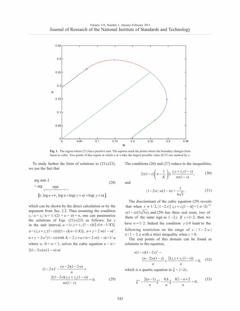
(v1( y + u) /u, v2 ( y + υ) /υ) ≥ y |u − υ | .Figure 1 shows the region where (21) has a positive
root in the (u, υ) plane. Its boundary is formed by twostraight segments where 3√3
−|u − υ | = 1, 3(u + υ) ≤ 1,
and by a cubic curve when u + υ ≥ 1/3. The largestpossible value of u or υ such that σ^ 2 > 0 is 8/27.
Volume 116, Number 1, January-February 2011Journal of Research of the National Institute of Standards and Technology
542
3 2 20 1 2 3 4
2 3 20 1 2 3 4
( )
( ) = 0.
c d d d d
d c c c c
υ υ υυ υ υ
+ + +
+ + + +
2 2 21 2 1 1 1 2 2 22 2 2 2 4 2 4
1 2 1 1 2 2
( )= = ,
( )x x n s n sν ν
σ σ σ σ σ σ−
− −+
3(2 ) 2( )( ) = 0,y u y u yυ υ+ + − + +
22 1 2( )ˆ .
4x xσ −
≤
31 , ( ) < 2 ,3
u u uυ υ υ+ ≥ +
2 22 1 2 1 20.391, = 0.860, = 0.075, = 0.102, 3 ,x s s n n− = =
there are three positive solutions,( = 0.2 63, = 0.053),= 0.138, = 0.106), ( = 0.035, = 0.312). In this
uu u
υυ υ
2ˆlikelihood evaluated when > 0, in which case theσstationary points are ( = = 0.065, = 0.230),u zυ( = 0.246, = 0.055, = 0.003), ( = 0.042, =0.234, = 0.019),( = 0.048, = 0.065, = 0.193) .u z u
z u zυ υ
υ
2 2 21 2ˆ ˆ ˆIf 0, the estimators , satisfy the equations,σ σ σ=
2 2 21 2ˆwhich imply the inequalities / < < [( )i i i is n x xν σ −
2 2 2 2 21 2 1 2 1 2 1 2ˆ ˆ ˆ ˆ2 ( ) ( ) .n x x n nσ σ σ σ− ≤ +
2 2 21 2ˆwhen > 0, in which case with = /( ) > 0,y x xσ σ −
21 1( ) 2( )( )( ) = 0,u u z u y u yυ ν υ− + − + +
22 2( ) 2( )( )( ) = 0.u z y u yυ υ ν υ υ− + − + +
2
2 2 2 2 2 21 1 2 2 1 2
ˆNotice that (21)-(23) imply that if > 0, then theˆ ˆ ˆ ˆinequalities , , and , are all s s
σσ σ σ σ≥ ≤ ≤
3( ) = (2 ) 2( )( ) .F y y u y u yυ υ+ + − + +
1 1< , | |< .3 3 3
u uυ υ+ −
2 21 2 1
2 2
[( ) /4 ] , = max(0, ). In this and only inˆthis situation (whose probability is zero), = . The
equation (21) implies that 2 1/2, so that i i
x x s x x
sy u
συ
+ +− −
+ + ≤
2 2 2 2 2 21 2 1 2 1ˆ ˆ ˆunless = , in which case = = , =s s sσ σ σ
2 2ˆ = ,i isσ
To study further the form of solutions to (21)-(23),we use the fact that
(28)
which can be shown by the direct calculation or by theargument from Sec. 2.2. Thus assuming the conditionz1 / u + z2 /υ + 1/ (2y + u + υ) = n, one can parametrizethe solutions of Eqs. (21)-(23) as follows: for sin the unit interval, u =
where w, 0 < w < 1, solves the cubic equation u − υ =
(29)
The conditions (26) and (27) reduce to the inequalities,
(30)
and
(31)
The discriminant of the cubic equation (29) reveals
following restriction on the range of s : | 1 − 2 w |≤ | 1 − 2 s| with a strict inequality when y > 0.
The end points of this domain can be found assolutions to the equation,
(32)
which is a quartic equation in ξ = 1−2s,
(33)
Volume 116, Number 1, January-February 2011Journal of Research of the National Institute of Standards and Technology
543
Fig. 1. The region where (21) has a positive root. The squares mark the points where the boundary changes fromlinear to cubic. Two points of this region at which u or υ take the largest possible value (8/27) are marked by o.
[ ]/ / 1/(2 )=1 2
1 2
arg min= arg min
log log log( ) log( ) ,z u z v y u v n
L
u y u yν ν υ υ+ + + +
+ + + + +
1 2( (1 ))/[ ( 1/ )],z s z s s n K+ − −2
1 2= ( (1 ))/[(1 )( 1/ )] , = 2 (1 ) ,z s z s s n K u y w wυ + − − − + −2= 2 (1 ) with = 2 = 2 (1 ) >1/ ,y w w K y u w w nυ υ+ − + + −
2(1 2 ) (1 ) orw w w− −
3
1 2
( 2)(1 2 )(1 2 )
2(1 2 )( (1 ))= 0.
(1 )
n wwn
s z s z sns s
− −− − +
− + −−
1 2 (1 )12 (1 ) ,(1 )
z s z ss s n
K ns s+ −⎛ ⎞− − ≥⎜ ⎟ −⎝ ⎠
1|1 2 | (1 ) < .6 3
w w w− −
3/21 2that when 1/ 2, |1 2 | [ (1 )] < ( 2)s s z s z s n≠ − + − −
(1 )/(3 3 ), and (29) has three real roots, two ofs s n−them of the same sign as 1 2 . 1/ 2, then wes If s− =have 1/ 2. Indeed the condition 0 leads to thew y= ≥
2
1 2
(1 )(1 2 )2( (1 ))( 2) (1 ) = 0,
s s sz s z sn s s
n n
− − −+ −− − +
4 22( 1) 8 8 2 = 0 .n z nn n n
ξ ξ ξ− Δ − +− − −
If the equation (33) has two distinct roots ξ_, ξ_
inthe interval (−1, 1), then the range of s-values is theinterval [s_, s
_], 0 < s_ = (1 − ξ
_) / 2 < s
_= (1−ξ_) / 2 < 1,
and for s ∈ (s_, s_
) the polynomial in (32) is negative.Therefore, if there are two roots of (29) in the interval(0, 1) which have the same sign as 1 − 2s, the one withthe smallest absolute value of |1 − 2w|, i.e., the one with
tions of equations (21)-(23) are parameterized by s∈ [s_, s_
]. To determine conditions for the equation (33) to have
two roots ξ_, ξ_
, in the interval (−1, 1), observe first thatit cannot have more than two roots there. Indeed thepolynomial in (33) assumes negative values at the endpoints, and it has exactly two roots if and only if thereis a point in this region at which that polynomial ispositive.
If the derivative of this polynomial, 4ξ 3− 4 (n − 1)ξ /n − 8Δ /n, does not vanish in (−1, 1), then (33)cannot have two roots there. This happens when thisderivative has just one real root, or equivalently thediscriminant of the cubic polynomial is negative whichmeans that | Δ | > [(n − 1) / (3n)]3/2 and which implies
that | Δ | > 1/2. Then the derivative takes negativevalues at the end points of the interval (−1, 1).
If ξ0 is the point of maximum of the polynomial (33)in (−1, 1), then 4ξ 0
3− 4(n − 1) ξ0 /n = 8Δ/n, and theroots ξ_, ξ
_exist if and only if
(34)
According to inequality (34),
(35)
(36)
Volume 116, Number 1, January-February 2011Journal of Research of the National Institute of Standards and Technology
544
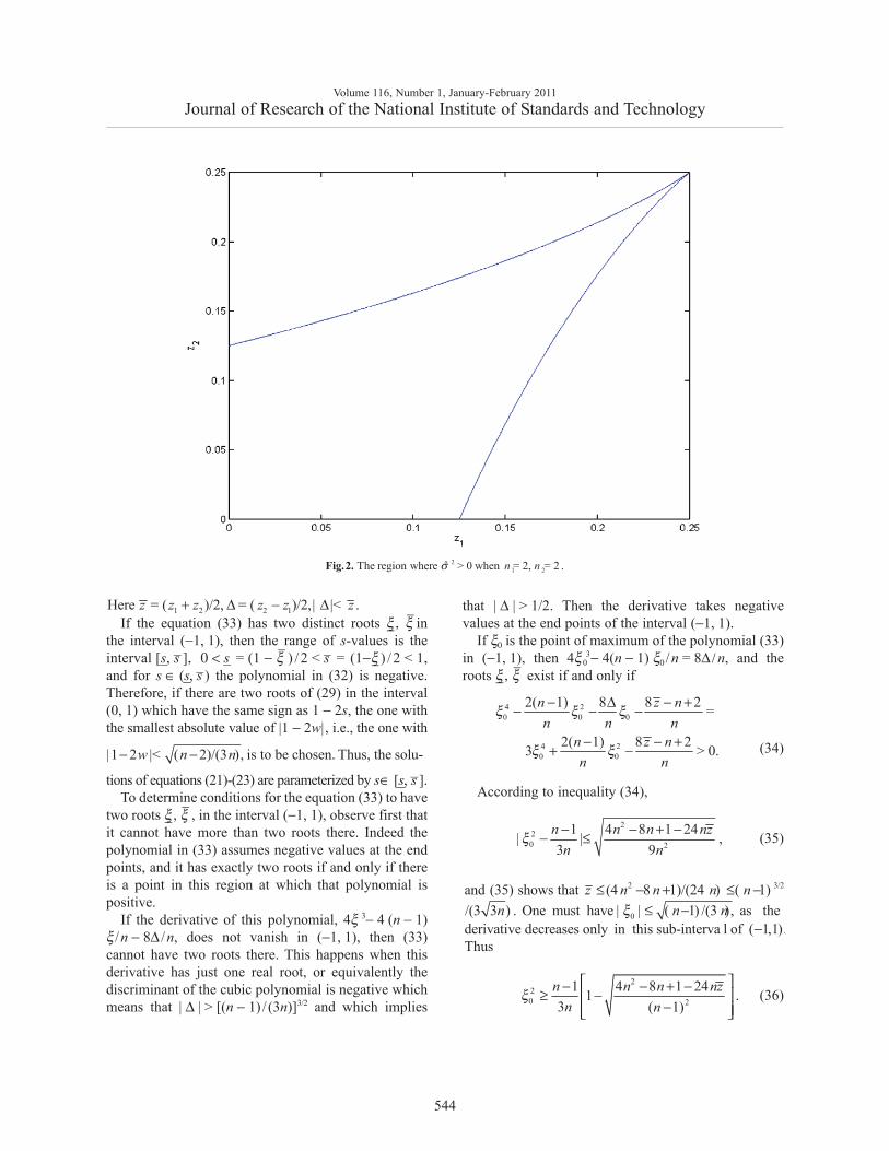
21 2ˆThe region where > 0 when = 2, = 2 .n nσFig.2.
1 2 2 1Here = ( )/2, = ( )/2,| |< .z z z z z z+ Δ − Δ
|1 2 |< ( 2)/(3 ), is to be chosen. Thus, the solu-w n n− −
4 20 0 0
4 20 0
2( 1) 8 8 2 =
2( 1) 8 23 > 0.
n z nn n n
n z nn n
ξ ξ ξ
ξ ξ
− Δ − +− − −
− − ++ −
220 2
1 4 8 1 24| | ,3 9
n n n nzn n
ξ − − + −− ≤
2 3/2
0
and (35) shows that (4 8 1)/(24 ) ( 1)/(3 3 ) . One must have | | ( 1) /(3 ), as thederivative decreases only in this sub-interva l of ( 1,1).Thus
z n n n nn n nξ
≤ − + ≤ −≤ −
−
220 2
1 4 8 1 241 .3 ( 1)
n n n nzn n
ξ⎡ ⎤− − + −≥ −⎢ ⎥
−⎢ ⎥⎣ ⎦
Volume 116, Number 1, January-February 2011Journal of Research of the National Institute of Standards and Technology
545
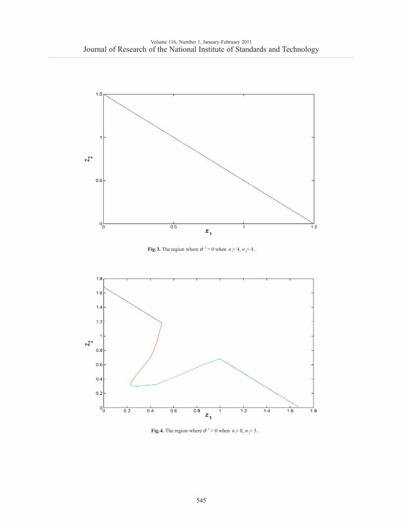
21 2ˆThe region where > 0 when = 4, = 4 .n nσFig.3.
21 2ˆThe region where > 0 when = 8, = 3 .n nσFig.4.
must have two roots ξ_, ξ_
as it takes a positive valuewhen ξ = 0. Since sign(ξ 0) = −sign (Δ), assuming that
(37)
which means that
(38)
The condition (38) can also be shown to be sufficientfor the existence of ξ_, ξ
_.
This parametrization and the Groebner basis for (13)allow for given z1, z2 to compare the minimal values of(9) when y > 0 with that when y = 0. Figures 2-4 showbounded regions where σ̂ 2 > 0 in the space (z1, z2) whenn1 = n2 = 2, n1 = n
2= 4, or n1 = 8, n2 = 3. When
n1 = n2≥ 3, this region is a triangle, z1 + z2 < c; for
n1 ≠ n2 it is more complicated.We summarize the obtained results.
Theorem 2.1. When p = 2, the Groebner basis for (13)is given by (16), (17). The solutions of (21)-(23) satisfyconditions (26) and (27). These solutions can beparametrized via (29) by s ∈ (s_, s
_) where the end points
can be found from (32) given that (38) holds.
We conclude by noticing the relationship of the prob-lem discussed here to the likelihood solutions to theclassical Behrens-Fisher problem [10] which assumesthat σ 2 = 0.
2.2 Solving Likelihood Equations Numerically
In view of the difficulty in evaluating the Groebnerbasis for p > 2, an iterative method to solve the opti-mization problem in (2) is of interest. Notice that thesum of the first two terms in (2) is a homogeneousfunction of σ 2, σ 1
2, …, σ p2, of degree −1. Therefore,
with n = ∑i ni ,
(39)
which reduces the problem to minimization of such
To minimize the objective function in (39)
(40)
one can impose a restriction on y0, y1, …, yp such as∑ yi = 1 or λ0 = 1. Note that F tends to +∞ whenyi → 0 or yi → +∞ for any fixed y0 > 0 . Since∑i (xi − μ
_) / (y0 + yi) = 0, one sees that
(41)
which must be positive for large yi and negative forsufficiently small yi .
Volume 116, Number 1, January-February 2011Journal of Research of the National Institute of Standards and Technology
546
2 2If 8 < 2 (i.e., 4 8 1 24 > ( 1) ), Eq. (33)z n n n nz n− − + − −
8 2, we getz n≥ −
20 0
3/2 2
2
1/22
2
2 | | 1= ( ) | |
1 4 8 1 2423 ( 1)
4 8 1 241 ,( 1)
nn n
n n n nzn n
n n nzn
ξ ξΔ − −
⎡ ⎤− − + −⎛ ⎞≥ +⎢ ⎥⎜ ⎟ −⎝ ⎠ ⎢ ⎥⎣ ⎦
⎡ ⎤− + −−⎢ ⎥−⎢ ⎥⎣ ⎦
2 3/2
2
3 2
(4 8 1 24 )3( 1)(4 8 1 24 )4[( 1) 27 ] 0 .
n n nzn n n nzn n
− + −+ − − + −≥ − − Δ ≥
( )
2 2 2 2 2 2, , , , , ,1 1
2 2
2 2 22 2 2, , , ,1
2 2 2
2
2 22 2 2, , ,1
22 2
2
=min min
( )= min
( )
log( ( )) log( )
( )1= [ (min min
) log ] log
l
p p
i i i
i ii ip
i i ii i
i
i ip
i ii
i ii
ii
L L
x s
x
sn
σ σ σ λσ λσ λσ
λ σ σ σ
λσ σ σ
μ νλ σ σ λσ
λ σ σ ν λσ
μλ σ σ
νλ σ σ
σ
ν
⎡ −+⎢ +⎣
⎤+ + + ⎥⎦⎡ −⎢ +⎣
+ + + +
+
∑ ∑
∑ ∑
∑
∑ ∑
∑
2
2 2
, , ,0 1 0
0
og
( )= logmin
log( ) log
log .
i
i i i
y y y i ip i i
i i ii i
x sn
y y y
y y y
n n n
σ
μ ν
ν
⎤⎥⎦
⎡ ⎛ ⎞−+⎢ ⎜ ⎟+⎢ ⎝ ⎠⎣
⎤+ + + ⎥⎦+ −
∑ ∑
∑ ∑
20 0
2
0 1
The minimizing value of is =( ( ) /( )/ )/ . Thus the objective function in (39)
becomes homogeneous of degree 0 in , , ,
i ii
i i ii
p
x y ys y n
y y y
λ λ μν
− ++
∑∑
0 1
2 2
0
0
( , , , )
( )= log
log( ) log ,
p
i i i
i ii i
i i ii i
F y y y
x sn
y y y
y y y
μ ν
ν
⎛ ⎞−+⎜ ⎟+⎝ ⎠
+ + +
∑ ∑
∑ ∑
2 2
2 20
2 20
0
( )( ) 1= ,
( )
i i i
i i i
i i ij j j
j j j
x sy y y
F ny y y yx s
y y y
μ νν
μ ν
− ++∂ − + +
∂ +⎡ ⎤−+⎢ ⎥+⎢ ⎥⎣ ⎦
∑
0 12 2 2
0 0 1 0 1 0
a function. If , , , is a solution to the problemˆ ˆ ˆ(39), then = , = , , = is a ML
solution.
p
p p
y y yy y yσ λ σ λ σ λ
If y0 > 0, by equating this derivative to zero, we obtain
(42)
The equation (42) must have a positive root, whichmeans that for λi evaluated at a stationary point,
(43)
and
(44)
It follows that for any stationary point, 2si2 > λ0yi, i.e.,
(45)
For a fixed value of λ0, say, λ0 = 1, the Eq. (42) leadsto an iteration scheme, with specified initial values ofy0
(0) and μ_
0. We take these to be the estimates arrived atby the method of moments as described later in Sec. 5,but once they are given, one can solve the cubicequation for υi = y0 / yi ,
(46)
It is easy to see that each of these equations haseither one or three positive roots. If there is just oneroot, then it uniquely defines υi. In case of three positiveroots, the root which minimizes (40) is chosen. Underthis agreement, at stage k in (46) υi = υi
(k), y0 = y0(k),
μ_
= μ_
k , and after solving (46) we put
(47)
and
(48)
k = 0, 1, ….
As in [11], (46) defines a sequence converging to astationary point, and at each step the value of (40) isdecreased.
Theorem 2.2 Successive-substitution iteration definedby equations (46), (47) and (48) converges to a station-ary point of (40) so that at each step thisfunction decreases. At any stationary point inequalities(43) and (44) hold and (45) is valid.
Notice that Vangel and Rukhin tacitly assume in [11]that y0 > 0. The case of the global minimum attainedat the boundary, i.e., when y0 = 0, can be handled asfollows. Equating (41) to zero gives
(49)
and a simpler version of an iterative scheme
(50)
k = 0, 1, …, yj(0) = sj
2, y0 = 0, converges fast. Howeverthe solutions obtained via (46), (47), (48) and (50)are to be compared by evaluating L. To assure that aglobal minimum has been found, several starting valuesshould be tried.
The maximum likelihood estimator and the restrict-ed maximum likelihood estimator discussed in the nextsection can be computed via their R-language imple-mentation through the lme function from nlme library[12]. However this routine has a potential (false orsingular) convergence problem occurring in somepractical situations.
Volume 116, Number 1, January-February 2011Journal of Research of the National Institute of Standards and Technology
547
20 0
20
= 0 ,i i i
i ii
s ny yyλ λ λ
ν−
− +
2 20 0where = ( ) /( ) / ,so that = .i i i i i i ix y y s y nλ μ ν λ λ− + + Σ
0 02 2
0
,4
i i i
i
y ns
ν λ λλ−
≥
2 20 0 0 0 0 0
2 20 0
= < .2 24 4
i i ii
i i i i ii i
n nsy s y s ys s
λ λ λ λ λ λ λν ν
−+ + + +
22 2
2
2
2 ˆ< < 2 .41 1
ˆ
ii i
i i
i
ss
n sσ
ν σ+ +
2 2 20
20
(1 ) (1 )
(1 ) ( ) = 0.i i i i i i
i i i
s y
y v x
υ υ ν υ νυ μ
+ − +
− + + −
( 1)
( 1)
1 ( 1)
( 1)
1= ,
1
kj j
kj j
k kj
kj j
xυυ
μυ
υ
+
+
+ +
+
+
+
∑
∑
( 1) 2( 1) 2 ( 1)10 ( 1)
( )1= ,1
kk ki i k
i i iki ii
xy s
nυ μ ν υ
υ
++ ++
+
⎡ ⎤−+⎢ ⎥+⎣ ⎦
∑ ∑
2 2( ),i i i
ii
x sy
nμ ν− +
∝
2 2
( 1)12 2
( )
1
( 1) ( 1)
( )
= ,( )
1= ,
i k i i
k ii k
j k j jk
j j
jk k
j jj j
x sn
yx s
y
xy y
μ ν
μμ ν
++
−
+ +
− +
− +
⎡ ⎤⎢ ⎥⎢ ⎥⎣ ⎦
∑
∑ ∑
3. Restricted Maximum Likelihood
The possible drawback of the maximum likelihoodmethod is that it may lead to biased estimators. Indeedthe maximum likelihood estimators of σ ’s do not takeinto account the loss in degrees of freedom that resultsfrom estimating μ. This undesirable feature is eliminat-ed in the restricted maximum likelihood (REML)method which maximizes the likelihood correspondingto the distribution associated with linear combinationsof observations whose expectation is zero. This methoddiscussed in detail by Harville [13] has gained consid-erable popularity and is employed now as a tool ofchoice by many statistical software packages.
The negative restricted likelihood function has theform
(51)
By using notation (5) and (6), we can rewrite
(52)
To estimate σ 2 and σi2, i = 1, …, p one has to find the
minimal value of Q /P′ + log P′. The derivative of thisfunction in σ 2 is proportional to the polynomial H ofdegree 2p−3 in this variable,
(53)
as opposed to 3p−3 which is the degree of the corre-sponding polynomial F in (12) under the ML scenario.
For fixed σi2, i = 1, …, p , all p roots of the poly-
nomial P = P (σ 2) are real numbers, so that
(54)
[14, 3.3.29].
An application of (54) shows that
(55)
Since P (σ 2) > 0, if F has a positive root σ 2, thenH also must have a positive root τ 2. Moreover,τ 2 ≤ σ 2, so that the ML estimator of σ 2 is always small-er than the REML estimator of the same parameter forthe same data.
The polynomial equations for the restricted likeli-hood method have the form,
(56)
with each of these polynomials being of degree 3 in σi2,
i = 1, …, p. When σ 2 > 0, Eqs. (56) have to be aug-mented by the equation H = 0.
3.1 Solving REML Equations
To solve the optimization problem in (51) in practiceone can use a method similar to that in Sec. 2.2. Indeed,
(57)
Volume 116, Number 1, January-February 2011Journal of Research of the National Institute of Standards and Technology
548
2 2 1
122 2 1
2 2 2 21 <
2 2 1 2 2
22
2
= log( ( ) ) =
( )( )
( )( )
log( ( ) ) log( )
log .
ii
i ji
i j p ii j
i ii i
i ii i
i ii
RL L
x x
s
σ σ
σ σσ σ σ σ
σ σ σ σ
ν ν σσ
−
−−
≤ ≤
−
+ +
− ⎡ ⎤+⎢ ⎥+ + ⎣ ⎦+ + + +
+ +
∑
∑ ∑
∑ ∑
∑ ∑
22
2= log log .i ii i
i ii
sQRL PP
νν σ
σ′+ + +
′ ∑ ∑
= ,H P P Q P QP′ ′′ ′ ′ ′′+ −
2 21[ ] [ ]pPP P Pp−′′ ′ ′≤ ≤
( ) = .F P P P Q P QP PH′ ′′ ′ ′ ′′≥ + −
4 2 2 2( ) ( )( ) = 0 ,i i i i i i iQ P QP PP s Pσ ν σ′ ′ ′ ′ ′ ′− + + −
2 2
2 2 22 2 2 2 2 2, , , , , , ,1 1
2 22 2
2
2 2
2 2 22 2 2, , ,1
2 2
( )=min min
( )
1log( ) log( ( ))( )
log( )
( )1= [ ( )min min
1( 1) log ] log
i i i
i ii ip p
ii ii
i ii
i i i
i ii ip
i i
x sRL
x s
n
σ σ σ λ σ σ σ
λσ σ σ
μ νλ σ σ λσ
λ σ σλ σ σ
ν λσ
μ νλ σ σ σ
λσ σ
⎡ −+⎢ +⎣
+ + ++
⎤+ ⎥⎦⎡ −
+⎢ +⎣
⎛+ − +
+⎝
∑ ∑
∑ ∑
∑
∑ ∑
∑
( )2 2
2
2 2
, , ,0 1 0
00
log
log
( )= ( 1) logmin
1log log( ) log
1 ( 1) log( 1) .
ii
i ii
i i i
y y y i ip i i
i i ii i ii
x sn
y y y
y y yy y
n n n
σ σ
ν σ
μ ν
ν
⎞+ +⎜ ⎟
⎠⎤+ ⎥⎦
⎡ ⎛ ⎞−− +⎢ ⎜ ⎟+⎢ ⎝ ⎠⎣
⎤⎛ ⎞+ + + + ⎥⎜ ⎟+ ⎥⎝ ⎠ ⎦+ − − − −
∑
∑
∑ ∑
∑ ∑ ∑
The minimizing value of λ is λ 0 = (∑i(xi−μ_
)2 /(y0 + yi) + ∑i visi
2 /yi) / (n−1), and the objective functionin (57) is homogeneous of degree 0 in y’s. Ify0, y1, …, yp is a solution to the problem (57), thenσ∼ 2 = λ0 y0, σ∼
12 = λ0 y1, …, σ∼
p2 = λ0 yp is a REML
solution.When y0 > 0, the function in (57) takes the form
(58)
Its derivative with respect to yi is
(59)
As in Sec. 2.2, for a fixed value λ0 = 1 we can use aniterative scheme which is based on (59). However, nowone has to specify initial values of y0
(0), μ_
0 and ofA(0) = ∑(y0 + yj)−1 after which the cubic equations forυi = y0 / yi ,
(60)
are solved for i = 1, …, p, with updating as in (47) and(48). Each of these equations has either one or threepositive roots. If there is just one root, then it definesvi , out of three roots the largest is taken.
If y = 0, then with the vectors e = (1, …, 1)T,z = (z1,…, (zp)T, zi = 1/σi
2, and p × p symmetric matrixdefined by positive elements ((xi − xj)2+vi si
2+vj sj2) /2,
(58) takes the form
(61)
The gradient of the function in (61)
(62)
and its Hessian is
(63)
where n→/ z is the vector with coordinates ni / zi ,i = 1, …, p, leads to the iteration scheme,
(64)
k = 0, 1, …, which converges fast.The solutions obtained via (60) and (64) are to be
compared by evaluating RL in (57).
3.2 REML p = 2
To find the REML solutions σ∼i2 and σ∼ 2 when p = 2
notice that (51) takes the form
(65)
which shows that if (x1 − x2)2 ≥ s12 + s2
2,
(66)
(67)
Indeed this choice simultaneously minimizes each ofthree bracketed terms in (65) guaranteeing the globalminimum at this point. When (x1 − x2)2 < s1
2 + s22, as we
will see, σ 2 = 0. To find σi2, i = 1, 2, one can employ
the Groebner basis of the polynomial equations (56)which in the notation of Sec. 2.1 takes the form
Volume 116, Number 1, January-February 2011Journal of Research of the National Institute of Standards and Technology
549
2 2
0
0 0
( )( 1) log
1 1log log log .
i i i
i ii i
i ii i ii i
x sn
y y y
yy y y y
μ ν
ν
⎛ ⎞−− +⎜ ⎟+⎝ ⎠
⎛ ⎞ ⎛ ⎞+ − +⎜ ⎟ ⎜ ⎟+ +⎝ ⎠ ⎝ ⎠
∑ ∑
∑ ∑ ∑
2 2
2 20
2 2
0
20
0
0
( )( )
( 1)( )
1( ) 1 .
1
i i i
i i
j i j
j j j
i i
i i
j j
x sy y y
nx sy y y
y yy y y
y y
μ ν
μ ν
ν
− ++
− −⎡ ⎤−
+⎢ ⎥+⎢ ⎥⎣ ⎦
+− + +
++
∑
∑
2 2 20 0
2
(1 ) (1 ) (1 )
/ ( ) = 0i i i i i i i
i i i
s y y
A x
υ υ ν υ ν υυ υ μ
+ − + − +
+ + −
, , >01
( 1) log( ) ( 2) log( ) log .min T Ti i
z z ip
n z z n z e n z⎡ ⎤− − − −⎢ ⎥⎣ ⎦∑
2( 1) ( 2) ,T T
n z e nnzz z z e
− − − −
22 2
2
2( 1) 4( 1) ( 2)=( ) ( )
.
T T
T T T
n n z z n eeFz z z z z e
ndiagz
− − −∇ − +
⎛ ⎞+ ⎜ ⎟⎝ ⎠
( )
( 1) ( ) ( )
2(0) ( )
2
2( 1) ( 2) ,( )
= , = 1 ,
k
k k T k
T kii
kk
n n z n ez z z
sz e z
s
+
−
−
−∝ − −
∑
22 21 2
1 22 21 2
2 22 21 2
1 1 2 22 21 2
( )= log(2 )
2
log log ,
x xRL y
y
s s
σ σσ σ
ν σ ν σσ σ
⎛ ⎞−+ + +⎜ ⎟+ +⎝ ⎠
⎛ ⎞ ⎛ ⎞+ + + +⎜ ⎟ ⎜ ⎟
⎝ ⎠ ⎝ ⎠
2 2= , = 1,2 ,i is iσ
2 2 2 21 2 1 2
1= ( ) .2
x x s sσ ⎡ ⎤− − −⎣ ⎦
(68)
(69)
This Groebner basis consists of three polynomials
(70)
whose coefficients are not needed here,
All stationary points of the restricted likelihoodequations can be found by solving the cubic equationG5 (υ) = 0 for υ > 0, and substituting this solution in(71), allowing one to express u through v,
Thus, in this case there are 3 complex non-zero rootspairs u, v.
Another approach is to use the argument in Sec. 3.1which for a fixed sum 2y0 + y1 + y2 = 1, leads to theoptimization problem,
(73)
If (x1 − x2)2 < s12 + s2
2, then according to Lemma 1 inthe Appendix, for a fixed sum y1 + y2 = y, the minimumin (73) monotonically decreases when 0 < y ≤ 1, so thatthis minimum is attained at the boundary, y1 + y2 = 1, inwhich case indeed σ∼ 2 = 0. Thus, one can solve thecubic equation for w = 1 − 2y1 ,
(74)
An alternative method is to use the iteration scheme(64) to solve (57).
4. Known Variances4.1 Conditions and Bounds for Strictly Positive
Variance Estimates
In view of the rather complicated nature of likeli-hood equations, in many situations it is desirable tohave a simpler estimating method for the commonmean μ. The most straightforward way is to assumethat the variances σi
2, i = 1, …, p, are known. In thiscase, essentially suggested in Ref. [15], but also pur-sued in Refs. [16, 17], these variances are taken to besi
2 (or a multiple thereof). Because of (3), the onlyparameter to estimate is y = σ 2.
Volume 116, Number 1, January-February 2011Journal of Research of the National Institute of Standards and Technology
550
2 21 1( 1) ( )( ) = 0u u u z uυ ν υ+ − + − +
2 22 2( 1) ( )( ) = 0 .v u z uυ ν υ υ+ − + − +
2 5 4 3 23 0 1 2 3 4( , ) = ,G u a u a a a aυ υ υ υ υ+ + + +
5 4 3 24 0 1 2 3 4
20 1 2 1 1 2 2 1 1 2 1
21 2 1 2
2 22 1 2 1 2 2 1 2 1
3 2 2 3 21 2 1 1 2 1 2 2 1
21 2 2 1
( , ) = ,
= 2 [ 2( 1) ( 2) 2],
= ( 1)( 2)( 2 2) ,
= ( 2 2) (2 2 4 2)
( 2 2)( 4 7 4 5
14 12 8 1
G u v b u b b b b
b n z n z z n z n z n
b n n n n n
b n n n n n n n z
n n n n n n n n n
n n n n
υ υ υ υ υ+ + + +
− + − + − + −
− − − + −
− + − + − − +
+ + − + + + −
− − + + 2 22 2 2
1 2 1 1 2 2 1 2
2 23 1 2 2 1
2 21 2 1 1 2 2 1 2 1 2
2 2 3 2 21 2 1 2 2 1 1 2 2 1
22 2
22 1 2 1 1 2
1 2 2
2 4)
( 2 2) ( 2 2 3 4 2),
= ( 2 2)
2( 2 2)( 2 2 3 4 2)
(3 6 4 12 12 4
12 4)
2 ( 2 2) 2( 2 2)
(2 2
n z
n n n n n n n n
b n n z
n n n n n n n n z z
n n n n n n n n n n
n z
n n z n n
n n n
ν
ν
−
+ + − + + − − +
− + −
+ + − + + − − +
− + + − − − +
+ −
− + − − + −
+ 21 2 2
22 1 2
4 1 2 1 2 1 2 1 1 2
1 2
6 5 4 35 0 1 2 3
0 2
21 2 1 2 1 2 1
2 21 2 1 2 1 2 2
2 21 2 1 2
4 2)
2 ( 2 2) ,
= (1 )[( 2 2) ( 2)
2 2],and
( , ) = ,with
= ( 1)( 2),
= (2 2 4 2)
( 3 4 3 6 2)
2 2
n n z
n n
b n z z z n n z n z
n n
G u c c c c
c n n n
c n n n n n z
n n n n n n z
n n n n
ν
υ υ υ υ υ
− − +
− + −
+ + + − + −
+ + −
+ + +
− −
+ − − +
− + + − − +
− − − + 1 22
2 2 1 1 2 1 2
21 2 2 2 1 1 2 2 2
23 2 1 2 1 2
3 4 2,
= (2 4 4)
(2 3 3) 2 (2 4 4) ,
= [( ) 2( ) 1] .
n n
c z n n z z
n n z z n n z
c z z z z z
νν ν
+ −
− + −
+ + − + + + − +
− − + + +
and
with
(71)
(72)
3 21 2 3 4 0= ( )/ .u b b b b bυ υ υ υ− + + +
1 2
11 2 1 2>0, >01 2
( 1) log 1 log ,min i iy y
y y
z zn y
y yν
+ ≤
⎡ ⎤⎛ ⎞− + + +⎢ ⎥⎜ ⎟
⎢ ⎥⎝ ⎠⎣ ⎦∑
3 2( 2) (4 2 ) ( 8 4 2)4 ( 1) 2 (1 4 ) = 0 ,
n w w n nz wn z
δ δδ
− − Δ + − + Δ − −− Δ − − +
2 1 1 2
2 1
where = ( )/2, and as before = ( )/2, =( )/2.
n n z z zz z
δ − + Δ−
We give here upper bounds on the ML estimatorσ^ 2 and on the REML estimator σ~ 2.
Theorem 4.1 Assume that the variances σi2,
i = 1, …, p, are known. Then
(75)
and
(76)
In particular, if
(77)
then σ^ 2 = 0. If
(78)
σ~ 2 = 0.Proof: We prove first that
(79)
Indeed, one can write
(80)
and Lemma 3 in the Appendix shows that since(p − 1 − ) | k − 1 − | ≤ (p − 1)(k − 1), (79) holds.
One gets for the polynomial H in (53),
(81)
which is positive under condition (78). Then σ~ 2 = 0.Similarly (77) and (54) imply that
(82)
To prove (76) observe that with y replaced by y + aa formula like (79) holds for any positive a. The onlymodification is that p − (σ1
2, …, σp2) is replaced by
p − (a + σ12, …, a + σp
2) and the H(k)(a) /k! representpolynomial coefficients. Then a version of Lemma 3 inthe Appendix states that
(83)
When p = 2, the bounds (75) and (76) are sharp as(24) and (67) show. When p increases, their accuracydecreases. Section 4.2 gives necessary and sufficientconditions for σ~ 2 = 0 when p = 3. It is possible to getbetter estimates under additional conditions. For exam-ple, if the ordering of sequences p − (σ−ij
2) (σi2 + σj
2)(notation of Lemma 2) and (xi − xj)2 (σi
2 + σj2)−1 is the
same, then the maximum of (xi − xj)2 (σi2 + σj
2),1 ≤ i < j ≤ p, in (77) and (78) can be replaced by theiraverage.
4.2 Example: Restricted Maximum Likelihood forp = 3
When p = 3, Q(y) = q0y + q1, is a polynomial ofdegree one, and
(84)
is a polynomial of degree three. If H(0) = h3 < 0, it hasa positive root, which means that σ~ 2 > 0. Otherwise theexistence of a positive root is related to the sign of thediscriminant
(85)
If D < 0 and h3 ≥ 0, there is just one real root whichmust be negative, and then σ∼ 2 = 0. If D ≥ 0, then thereare three real roots. The condition h3 ≥ 0 implies thateither two of them are positive and one is negative (sothat at least one of the coefficients h1 or h2 is negative)and σ∼ 2 > 0, or all three roots are negative (so thatσ∼ 2 > 0.)
Volume 116, Number 1, January-February 2011Journal of Research of the National Institute of Standards and Technology
551
2 22 2 2( 1) ( )1ˆ ( ) ,max
2i j
i ji j
p x xp
σ σ σ≠
+
⎡ ⎤− −≤ − +⎢ ⎥
⎢ ⎥⎣ ⎦
2 2 2 21 ( 1)( ) ( ) .max2 i j i j
i jp x xσ σ σ
+≠⎡ ⎤≤ − − − +⎣ ⎦
2
2 2 21 <
( ),max
( 1)i j
i j p i j
x x ppσ σ≤ ≤
−≤
+ −
2
2 21 <
( ) 1 ,max1
i j
i j p i j
x xpσ σ≤ ≤
−≤
−+
2
2 21 <
( )| | ( 1) .max i j
i j p i j
x xQP Q P p P P
σ σ≤ ≤
−′′ ′ ′ ′ ′′− ≤ −
+
22
,
= ( 1 ) ,kp p k
kQP Q P k k q y + −
− − −′′ ′ ′− − −∑
2
2 21 <
( )1 ( 1) ,max i j
i j p i j
x xH P P p
σ σ≤ ≤
⎡ ⎤−′ ′′≥ − −⎢ ⎥
+⎢ ⎥⎣ ⎦
22
2 21 <
( )( ) ( 1) 0 .max i j
i j p i j
x xF P P p PP
σ σ≤ ≤
⎡ ⎤−′ ′ ′′≥ − − ≥⎢ ⎥
+⎢ ⎥⎣ ⎦
( )
2 ( 1)
2 21 <
2 ( 1)
2 21 <
( ) ( 1)( 1)!
( ) ( )max
( 1)!2
( ) ( )= ( 1) .max!2
i j
i j p i j
i j
i j p i j
Q a p
x x P aa
x x P apa
σ σ
σ σ
+
≤ ≤
+
≤ ≤
≤ + − −
⎡ ⎤−⎢ ⎥
++ +⎢ ⎥⎣ ⎦
⎡ ⎤−− − ⎢ ⎥
+ +⎢ ⎥⎣ ⎦
2 2 2 11 <
( ) 2
1 2
2 2
The argument, as before, shows now that if( ) / (2 ) ( 1) , thenmax
( ) 0, = 0, , 2 3 . It follows that ,so that (76) is valid with = 2 m ax[( 1)( )
( )] . The proof of (75) is similar
i j i ji j pk
i j
i j
x x a pH a k p a
a p x x
σ σσ
σ σ
−≤ ≤
−
+
− + + ≤ −≥ − ≤
− −− +
. +
3 21 0
22 1 1 2 1 0 2 1 1
3
30
( ) = 18 3(6 )
(6 4 6 ) 2 2
= kk
H y y q y
q y q q
h y−
+ −
+ + − + + −
∑
2 2 3 31 2 0 2 1 3
2 20 3 0 1 2 3
= 4 427 18 .
D h h h h h hh h h h h h− −
− +
Separation between these cases depends on the ratio
the proof of Theorem 4.1, E1 ≥ λ , but we do not usethis fact here.
h2 = 0, i.e., when E2 = λ −2 E12/3, D factorizes as fol-
(86)
which is defined for λ < 0.5137…, and let E
1 be the(only) positive root of the equation
(87)
The discriminant of (87) is negative, and accordingto Descartes’s rule there are always two complex roots,and one positive root. It is easy to check that E
1 = E
1(λ)is monotonically increasing in λ < 0 and E
1(1/16) = 1/4.In this notation, when λ ≤ 1/16 (so that h2 ≤ 0
implies that h1 ≤ 0), the region {(E1, E2) : E2 ≤ E12/3,
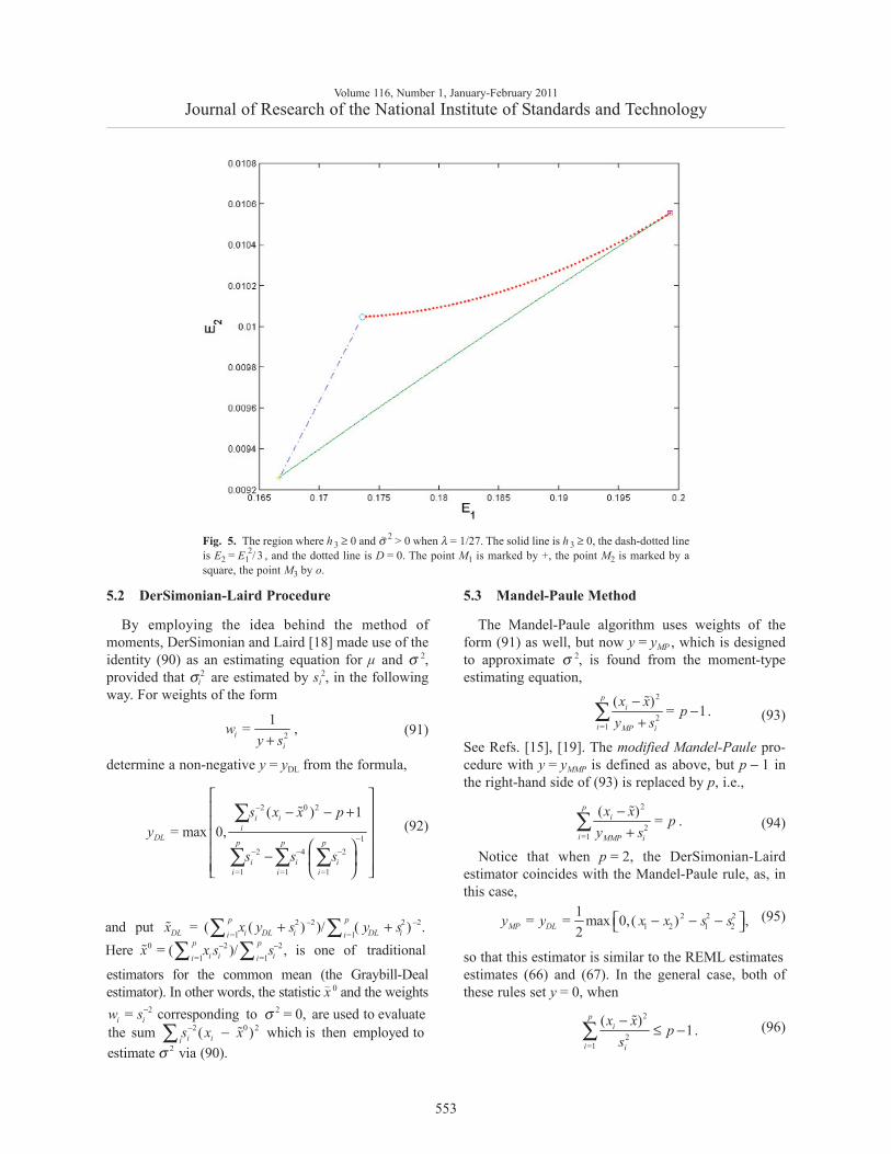
h3 ≥ 0, σ∼ 2 > 0}, is formed by three curves: (i ) h3 = 0
between the point
but the probability of having the likelihood solutionthere is zero.
5. Moment-Type Equations5.1 Weighted Means Statistics
When the within-lab and between-lab variances σi2
and σ 2 are known, the best (in terms of the meansquared error) unbiased estimator of the treatmenteffect μ in the model (1) is a weighted means statistic(3) with wi = wi
0 = 1 / (σ 2 + σi2 ). Even without the
normality assumption for these optimal weights,E ∑i wi
0 (xi − μ− )2 = p − 1, and
(88)
If V ar(xi) = σi2 + σ 2, but the weights wi are arbitrary,
(89)
In particular, when wi = 1/σi2
(90)
The simplest estimate of the within-trials vari-ances σi
2 is by the available si2 , but the problem of
estimating the between-trial component of varianceσ2 remains.
Volume 116, Number 1, January-February 2011Journal of Research of the National Institute of Standards and Technology
Algebra shows that when = /3, one has =544( 3 ) (3 1/16 ) , when = 0, i.e., if
= /( 0.5), then = 36(4 3 )(8 20 10 1 48 )(1 2 ) , and on the curve
E E DE E h
E E E D E EE E E E
λ λλ λ
λ −
− + −+ + −
− − + + +
3 21 1 18 20 10 1 48 = 0 ,E E E λ− − + +
3 21 14 2 3 = 0 .E E λ+ −
1 = (( 1 48 1)/4, (1 24M λ λ+ − + −
3 22 2
1 1 1 22
1 1 2 12 2
1 2 1
2
1 48 )/24), where = 0 intersects the curve =/3, and the point ( , 2 /3) on = 0,/3 between and the point = ( = 3 1/6,/3) where 0 intersects = /3,
the cubic in curve corresponding to the equatio n0, w
h EE E E hE M M EE D E E
ED
λλ
λ
+−
+=
=
2 32
1
3 1 1
hich connects the point and the point =(3 1/6, /3). See Fig. 5. If 2 /81, this region also
ˆincludes the part of the curve = 0 where ,
M ME
h E Eλ λ+ <
≤
1 1
1 2 1 22
3
When 1/16, one has 1/ 4 (1/16), so that0. Also then /3, , so that 0.
Thus in this situation 0 if and only if 0.
E Eh E E h
h
λλ λσ
> > => > > >
> ≥
20 2 2 1
1 1( ) = = .( )i i
i i
Ew
μ μσ σ −−
+∑ ∑
2 2 2
2 2 2 1
1
1
2 2 2
2 21 1
1 1
1 1
( )( ) = ( )
= .
p
i ip
i i i i pi
i
p p
i i ip p
i i ip p
i i
wE w x w
w
w ww w
w w
σ σμ σ σ
σσ σ
+− + −
⎡ ⎤⎢ ⎥⎢ ⎥− + −⎢ ⎥⎢ ⎥⎣ ⎦
∑∑ ∑
∑
∑ ∑∑ ∑
∑ ∑
2 412
2 21
21
1( ) 1= 1 .
1
p
pi i
pi i i
i
xE p
μ σσ
σ σσ
⎡ ⎤⎢ ⎥− ⎢ ⎥− + −⎢ ⎥⎢ ⎥⎣ ⎦
∑∑ ∑
∑
3 2 3 21 1 1 1 1
1
lows, = 36(4 2 3 ) (108 162 18ˆ81 ). Let be the smallest positive root of the
cubic equation
D E E E E EE
λλ
+ − − −+
2( )i i E =
and by ( ) i i i
5.2 DerSimonian-Laird Procedure
By employing the idea behind the method ofmoments, DerSimonian and Laird [18] made use of theidentity (90) as an estimating equation for μ and σ 2,provided that σi
2 are estimated by si2, in the following
way. For weights of the form
(91)
determine a non-negative y = yDL from the formula,
(92)
estimators for the common mean (the Graybill-Dealestimator). In other words, the statistic x~ 0 and the weights
5.3 Mandel-Paule Method
The Mandel-Paule algorithm uses weights of theform (91) as well, but now y = yMP , which is designedto approximate σ 2, is found from the moment-typeestimating equation,
(93)
See Refs. [15], [19]. The modified Mandel-Paule pro-cedure with y = yMMP is defined as above, but p − 1 inthe right-hand side of (93) is replaced by p, i.e.,
(94)
Notice that when p = 2, the DerSimonian-Lairdestimator coincides with the Mandel-Paule rule, as, inthis case,
(95)
so that this estimator is similar to the REML estimatesestimates (66) and (67). In the general case, both ofthese rules set y = 0, when
(96)
Volume 116, Number 1, January-February 2011Journal of Research of the National Institute of Standards and Technology
553
Fig. 5. The region where h 3 ≥ 0 and σ∼ 2 > 0 when λ = 1/27. The solid line is h 3 ≥ 0, the dash-dotted lineis E2 = E1
2/ 3 , and the dotted line is D = 0. The point M1 is marked by +, the point M2 is marked by asquare, the point M3 by o.
2
1= ,ii
wy s+
2 0 2
12 4 2
=1 =1 =1
( ) 1= max 0,
i ii
DL p p p
i i ii i i
s x x py
s s s
−
−− − −
⎡ ⎤⎢ ⎥− − +⎢ ⎥⎢ ⎥⎛ ⎞⎢ ⎥− ⎜ ⎟⎢ ⎥⎝ ⎠⎣ ⎦
∑
∑ ∑ ∑
2 2 2 2=1 =1
0 2 2=1 =1
and put = ( ( ) )/ ( ) .Here = ( )/ , is one of traditional
p pDL i DL i DL ii i
p pi i ii i
x x y s y sx x s s
− −
− −
+ +∑ ∑∑ ∑
2
2=1
( )= 1.
pi
i MP i
x xp
y s−
−+∑
2
2=1
( )= .
pi
i MMP i
x xp
y s−
+∑
2 2 21 2 1 2
1= = max 0,( ) ,2MP DLy y x x s s⎡ ⎤− − −⎣ ⎦
2
2=1
( )1.
pi
i i
x xp
s−
≤ −∑ 2 2
2 0 2
2
= corresponding to = 0, are used to evaluatethe sum ( ) which is then employed toestimate via (90).
i i
i ii
w ss x x
σ
σ
−
− −∑
It was shown in Ref. [20] that the modified Mandel-Paule is characterized by the following fact: the MLestimator σ^ 2 of σ 2 coincides with yMMP , if in the repa-rametrized version of the likelihood equation theweights wi admit representation (91). As a conse-quence, the corresponding weighted means statistic (3)must be close to the ML estimator, so that the modifiedMandel-Paule estimator approximates its ML counter-part. Thus, the modified Mandel-Paule estimator can beinterpreted as a procedure which uses weights of theform 1 / (y + si
2), instead of solutions of the likelihoodequation that are more difficult to find, and still main-tains the same estimate of σ 2 as ML.
A similar interpretation holds for the originalMandel-Paule rule and the REML function [21]. Forthis reason both Mandel-Paule rules are quite natural. Itis also suggestive to use the weights (91) withy = yMP determined from the Mandel-Paule equation(93) as a first approximation when solving thelikelihood equations via the iterative scheme (47) and(48).
5.4 Uncertainty Assessment
It is tempting to use formula (88) to obtain an estima-tor of the variance of x~ . For example, DerSimonian andLaird [18] suggested an approximate formula for theestimate of the variance of their estimator,
(97)
Similarly motivated by (88), Paule and Mandel [19]suggested to use [∑i (yMP + si
2)−1]−1 to estimate thevariance of x~MP . However these estimators typicallyunderestimate the true variance, Ref. [5]. They are notGUM consistent [22] in the sense that the variance esti-mate is not representable as a quadratic form in devia-tions xi − x~ .
Horn, Horn and Duncan [23] in the more generalcontext of linear models have suggested the followingGUM consistent estimate of V ar (x~), which has theform ∑i ωi
2 (xi − x~ )2 / (1 − ωi), with ωi = wi / ∑k wk .When the plug-in weights are ωi = (y + si
2)−1 /∑k (y + sk
2)−1, i = 1, …, p, this estimate is
(98)
Simulations show that (98) gives good confidence in-
Paule rule or the DerSimonian-Laird procedure they
when all sample means are close xi ≈ x~ , then yDL = 0and the uncertainty estimate (∑i si
−2)−1 may be a moresatisfactory answer than δ ≈ 0.
When p = 2,
(99)
In this case δ is an increasing function of y with thelargest value (x1 − x2)2 /4 attained when y → ∞.
An alternative method of obtaining confidenceintervals for μ on the basis of REML estimators wassuggested in Ref. [24] for an adjusted estimator of
based on the inverse of the Fisher informa-tion matrix. This (not GUM consistent) estimator ismore complicated.
6. Conclusions
The original motivation for this work was an attemptto employ modern computational algebra techniques byevaluating the Groebner bases of likelihood polynomi-al equations for the random effects model. While thisattempt leads to an explicit answer when there are twolabs with no between-lab effect, it was not successful ina more general situation. The classical iterative algo-rithms appear to be more efficient in this applicationalthough they do not guarantee the global optimum.Simplified, method of moments based procedures,especially the DerSimonian-Laird method, deservemuch wider use in interlaboratory studies.
Volume 116, Number 1, January-February 2011Journal of Research of the National Institute of Standards and Technology
554
2 1
1( ) = .( )DL
DL ii
Var xy s −+∑
/ 2 2tervals of the form, ( 1) . For the Mandel-x t pα δ± −
/2outperform the intervals, ( 1) ( ). StillDLx t p Var xα± −
2 2 21 2 1 2
2 2 21 2
( ) ( )( )= .
(2 )x x y s y s
y s sδ − + +
+ +
( )Var μ
12
2 2 2:
2
( ) 1( )
= .1
i
i k k ii k
i i
x xy s y s
y s
δ
−
≠
⎡ ⎤−⎢ ⎥+ +⎣ ⎦
+
∑ ∑
∑
7. Appendix7.1 Lemma 1
(100)
is monotonically nondecreasing in the interval (0, 1)
Proof: With B = (1 + z1 / y1 + z2 / y2) / (n − 1), anystationary point (y1, y2) in (100) satisfies the simultane-ous equations,
(101)
where ζ is the Lagrange multiplier. By multiplyingthese equations by y1 and y2 respectively and addingthem, we see that ζ y = 1 − 1/B. Notice that B ≤ 1 ifand only if ζ ≤ 0, which means that B ≥ zi / (vi yi) fori = 1, 2. Then z1 /v1 + z2 /v2 ≤ 1, which contradicts thecondition of the Lemma 1. Therefore, B > 1.
To prove Lemma 1 it suffices to show that the deriv-ative of (100) is negative. This fact follows from theinequality
(102)
which can be proven by differentiation of (101). Indeedfor i = 1, 2,
(103)
Since y1 + y2 = y, and y′1 + y′2 = 1, by adding these iden-tities we get
(104)
7.2 Elementary Symmetric Polynomials:Lemmas 2 and 3
We note the following identities for elementarysymmetric polynomials.
(105)
Comparison of the coefficients of the polynomial
(106)
By differentiating the identity,
(107)
Combined with (105), identities (106) and (107)demonstrate the following formula (108) (which theauthor was unable to find in the literature.)
Lemma 2 Under the notation above, for
(108)
The following result Lemma 2 gives an upper boundon the coefficients of polynomial Q.
Lemma 3 For = 0, 1, , …, p − 2,
(109)
Volume 116, Number 1, January-February 2011Journal of Research of the National Institute of Standards and Technology
[1] W. G. Cochran, Problems arising in the analysis of a series ofsimilar experiments, J. Royal Statist. Soc. Supplement 4, 102-118 (1937).
[2] W. G. Cochran, The combination of estimates from differentexperiments, Biometrics 10, 101-129 (1954).
[3] P. S. R. S. Rao, J. Kaplan, and W. G. Cochran, Estimators forthe one-way random effects model with unequal error vari-ances, J. Am. Stat. Assoc. 76, 89-97 (1981).
[4] P. S. R. S. Rao, Cochran’s contributions to variance componentmodels for combining estimates, in P. Rao and J. Sedransk,edis., W. G. Cochran’s Impact on Statistics, Wiley, New York,(1981), pp. 203-222.
[5] A. L. Rukhin, Weighted means statistics in interlaboratorystudies, Metrologia 46, 323-331 (2009).
[6] D. R. Cox, Combination of data, in Encyclopedia of StatisticalSciences, Vol 2, S. Kotz, C. B. Read, N. Balakrishnan, andB. Vidakovic, eds., Wiley, New York (2006), pp. 1074-1081.
[7] E. F. Beckenbach and R. Bellman, Inequalities, Springer,Berlin, (1961), p. 3.
[8] D. Cox, J. Little, and D. O’Shea, Ideals, Varieties andAlgorithms, 2nd ed, Springer, New York (1997), pp. 96-97.
[9] M. Drton, B. Sturmfels, and S. Sullivant, Lectures on AlgebraicStatistics, Birkhauser, (2009), pp. 15-55.
[10] A. Belloni and G. Didier, On the Behrens-Fisher problem: aglobally convergent algorithm and a finite-sample study of theWald, LR and LM tests, Ann. Statist. 36, 2377-2408 (2008).
[11] M. G. Vangel and A. L. Rukhin, Maximum likelihood analysisfor heteroscedastic one-way random effects ANOVA in inter-laboratory studies, Biometrics 55, 129-136 (1999).
[12] R Development Core Team R: A language and environment forstatistical computing, R Foundation for Statistical Computing,Vienna, Austria (2009) ISBN 3-900051-07-0, URLhttp://www.R-project.org.
[13] D. Harville, Maximum likelihood approaches to variance com-ponents estimation and related problems, J. Am. Stat. Assoc.72, 320-340 (1977).
[14] D. S. Mitrinovich, Analytic Inequalities, Springer, Berlin,(1970) p 227.
[15] J. Mandel and R. C. Paule, Interlaboratory evaluation of amaterial with unequal number of replicates, Anal. Chem. 42,1194-1197 (1970).
[16] R. Willink, Statistical determination of a comparison referencevalue using hidden errors, Metrologia 39, 343-354 (2002).
[17] E. Demidenko, Mixed Models, Wiley, New York, (2004), pp.253-255.
[18] R. DerSimonian and N. Laird, Meta-analysis in clinical trials,Control. Clin. Trials 7, 177-188 (1986).
[19] R. C. Paule and J. Mandel, Consensus values and weightingfactors, J. Res. Natl. Bureau Stand. 87, 377-385 (1982).
[20] A. L. Rukhin and M. G. Vangel, Estimation of a common meanand weighted means statistics, J. Am. Stat. Assoc. 93, 303-308(1998).
[21] A. L. Rukhin, B. Biggerstaff, and M. G. Vangel, Restrictedmaximum likelihood estimation of a common mean andMandel-Paule algorithm, J. Stat. Plann. Inf. 83, 319-330(2000).
[22] International Organization for Standardization, Guide to theExpression of Uncertainty in Measurement. Geneva,Switzerland, (1993).
[23] S. A. Horn, R. A. Horn, and D. B. Duncan, Estimatingheteroscedastic variance in linear models. J. Am. Stat. Assoc.70, 380-385 (1975).
[24] M. G. Kenward and J. H. Roger, Small sample inference forfixed effects from restricted maximum likelihood. Biometrics,53, 983-997 (1997).
About the author: Andrew L. Rukhin is a Mathe-matical Statistician in the Statistical EngineeringDivision of the NIST Information TechnologyLaboratory. He got his M.S. in Mathematics (Honors)from the Leningrad State University (Russia) in 1967and his Ph.D. from the Steklov Mathematical Institutein 1970. After emigrating from the USSR he worked asa professor at Purdue University (1977-1987), atUniversity of Massachusetts, Amherst (1987-1989) andat the University of Maryland at Baltimore County(1989-2008). Now Rukhin is a Professor Emeritus atthis university. Rukhin is a Fellow of the Institute ofMathematical Statistics, and a Fellow of the AmericanStatistical Association. He won Senior DistinguishedScientist Award By Alexander von Humboldt-Foundation in 1990, and the Youden Prize forInterlaboratory Studies in 1998 and in 2008. TheNational Institute of Standards and Technology is anagency of the U.S. Department of Commerce.
Volume 116, Number 1, January-February 2011Journal of Research of the National Institute of Standards and Technology


![HITRUST CSF Risk FactorsTypical risk factors include threat, vulnerability, impact, likelihood, and predisposing condition [emphasis added]. 16 NIST defines a predisposing condition](https://static.documents.pub/doc/80x56/6006edc4ec5cc202641ec6f7/hitrust-csf-risk-factors-typical-risk-factors-include-threat-vulnerability-impact.jpg)


![Restricted maximum likelihood estimation of covariances in ...neum/ms/reml.pdf · In 1987 Graser et al. [18] introduced the derivative free optimization, which in the following years](https://static.documents.pub/doc/80x56/6067c918988aa736b30045d3/restricted-maximum-likelihood-estimation-of-covariances-in-neummsremlpdf.jpg)
