56
MBA7020_07.ppt/July 11, 2005/Page 1 Georgia State University - Confidential MBA 7020 Business Analysis Foundations Simulation July 11, 2005
| Date post: | 19-Dec-2015 |
| Category: |
Documents |
| View: | 214 times |
| Download: | 0 times |
MBA7020_07.ppt/July 11, 2005/Page 1Georgia State University - Confidential
MBA 7020
Business Analysis Foundations
Simulation
July 11, 2005
MBA7020_07.ppt/July 11, 2005/Page 2Georgia State University - Confidential
Agenda
Simulation with Crystal
Ball
Spreadsheet Simulation
What is Simulation
MBA7020_07.ppt/July 11, 2005/Page 3Georgia State University - Confidential
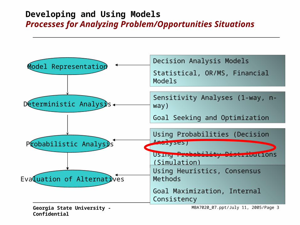
Developing and Using Models Processes for Analyzing Problem/Opportunities Situations
Model Representation
Deterministic Analysis
Probabilistic Analysis
Evaluation of Alternatives
Decision Analysis Models
Statistical, OR/MS, Financial Models
Sensitivity Analyses (1-way, n-way)
Goal Seeking and Optimization
Using Probabilities (Decision Analyses)
Using Probability Distributions (Simulation)
Using Heuristics, Consensus Methods
Goal Maximization, Internal Consistency
MBA7020_07.ppt/July 11, 2005/Page 4Georgia State University - Confidential
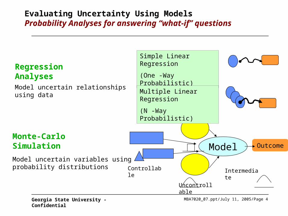
Evaluating Uncertainty Using Models Probability Analyses for answering “what-if” questions
Controllable
Uncontrollable
Intermediate
Model Outcome
Regression Analyses
Simple Linear Regression
(One -Way Probabilistic)
Multiple Linear Regression
(N -Way Probabilistic)
Model uncertain relationships using data
Monte-Carlo Simulation
Model uncertain variables using probability distributions
MBA7020_07.ppt/July 11, 2005/Page 5Georgia State University - Confidential
What is Simulation?
• Modeling a real system to learn about its behavior
• The model is a set of mathematical and logical relationships
• You can vary conditions to test different scenarios
MBA7020_07.ppt/July 11, 2005/Page 6Georgia State University - Confidential
Advantages / Disadvantages
Advantages of Simulation
• Inexpensive to evaluate decisions before implementation
• Reveals critical components of the system
• Excellent tool for selling the need for change
Disadvantages of Simulation
• Results are sensitive to the accuracy of input data• Garbage in, Garbage out• Intelligent agents using secret rules
• Investment in time and resources
MBA7020_07.ppt/July 11, 2005/Page 7Georgia State University - Confidential
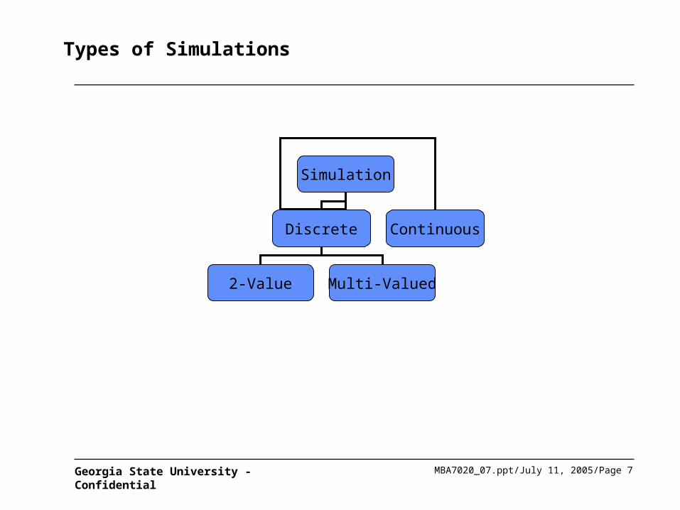
Types of Simulations
Simulation
Discrete Continuous
2-Value Multi-Valued
MBA7020_07.ppt/July 11, 2005/Page 8Georgia State University - Confidential
Simulating with a Spreadsheet
• Simulations can be performed with spreadsheets alone. However, add-in software packages can enhance the capabilities of Excel.
• Two Excel add-in packages that will be used are Crystal Ball and @Risk.
• These add-ins offer additional random distributions and easy commands to set up and run many more iterations than could be run in Excel.
• In addition, they automatically gather statistical and graphical summaries of the results.

MBA7020_07.ppt/July 11, 2005/Page 9Georgia State University - Confidential
Agenda
Spreadsheet Simulation
Simulation with Crystal
Ball
What is Simulation

MBA7020_07.ppt/July 11, 2005/Page 10Georgia State University - Confidential
A Capital Budgeting Example: Adding A New Product LineSpreadsheet: Spreadsheet_Simulation.xls
• Airbus Industry is considering adding a new jet airplane (model A3XX) to its product line. The following financial information is available:
• Tax depreciation on the new equipment would be $10,000 per year over the 4 year expected product life.
• Salvage value of the equipment at the end of the 4 years is estimated to be 0.
• Airbus’ cost of capital is 10% and tax rate is 34%.
Startup CostsStartup Costs $150,000$150,000Sales PriceSales Price $ 35,000$ 35,000Fixed Costs (per year)Fixed Costs (per year) $ 15,000$ 15,000Variable Costs (per year) 75% of revenuesVariable Costs (per year) 75% of revenues

MBA7020_07.ppt/July 11, 2005/Page 11Georgia State University - Confidential
If demand is known, then a spreadsheet can be used to calculate the net present value (NPV). For example, assume that the demand for A3XXs is 10 units for each of the next 4 years:
=C9*$B$3=$B$4
=C10*$D$2=$B$5
=C10-SUM(C11:C13)=$D$4*C14=C14 – C15=C16 + C13
=-$B$2
=NPV($D$3,C17:F17)+B17
MBA7020_07.ppt/July 11, 2005/Page 12Georgia State University - Confidential
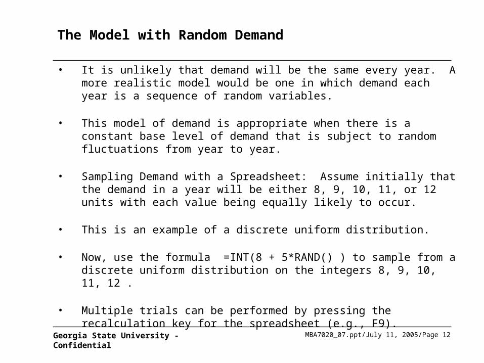
The Model with Random Demand
• It is unlikely that demand will be the same every year. A more realistic model would be one in which demand each year is a sequence of random variables.
• This model of demand is appropriate when there is a constant base level of demand that is subject to random fluctuations from year to year.
• Sampling Demand with a Spreadsheet: Assume initially that the demand in a year will be either 8, 9, 10, 11, or 12 units with each value being equally likely to occur.
• This is an example of a discrete uniform distribution.
• Now, use the formula =INT(8 + 5*RAND() ) to sample from a discrete uniform distribution on the integers 8, 9, 10, 11, 12 .
• Multiple trials can be performed by pressing the recalculation key for the spreadsheet (e.g., F9).
MBA7020_07.ppt/July 11, 2005/Page 13Georgia State University - Confidential
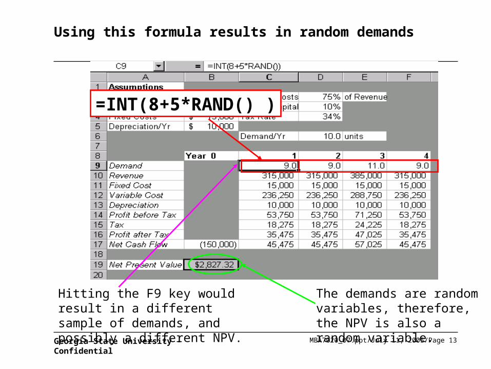
=INT(8+5*RAND() )
Using this formula results in random demands
Hitting the F9 key would result in a different sample of demands, and possibly a different NPV.
The demands are random variables, therefore, the NPV is also a random variable.
MBA7020_07.ppt/July 11, 2005/Page 14Georgia State University - Confidential
Evaluating The Proposal
• Two questions need to be answered about the NPV distribution:
1. What is the mean or expected value of the NPV?
2. What is the probability that the NPV assumes a negative value (making the proposal to add the A3XX less attractive)?
• To answer these questions, a simulation model must be built. To run the simulation automatically and capture the resulting NPV in a separate spreadsheet, use the Data Table command.

MBA7020_07.ppt/July 11, 2005/Page 15Georgia State University - Confidential
Start with a blank worksheet by clicking on the Insert menu and select Worksheet
Next, rename this blank worksheet 100 Iterations

MBA7020_07.ppt/July 11, 2005/Page 16Georgia State University - Confidential
Type the starting value (1) in cell A2 and hit Enter, then return to cell A2.
Click the Edit menu and choose Fill – Series.
In the resulting dialog, select Series in Columns and enter a stop value of 100. Click OK to fill series.
MBA7020_07.ppt/July 11, 2005/Page 17Georgia State University - Confidential
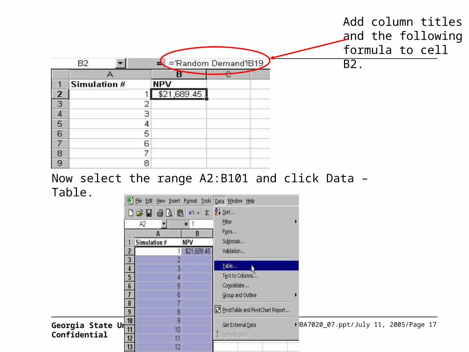
Add column titles and the following formula to cell B2.
Now select the range A2:B101 and click Data – Table.
MBA7020_07.ppt/July 11, 2005/Page 18Georgia State University - Confidential
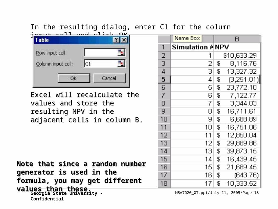
In the resulting dialog, enter C1 for the column input cell and click OK.
Note that since a random number Note that since a random number generator is used in the formula, you generator is used in the formula, you may get different values than these.may get different values than these.
Excel will recalculate the values and Excel will recalculate the values and store the resulting NPV in the store the resulting NPV in the adjacent cells in column B. adjacent cells in column B.
MBA7020_07.ppt/July 11, 2005/Page 19Georgia State University - Confidential
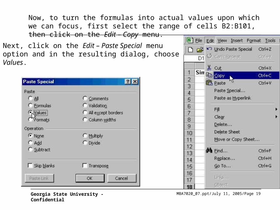
Now, to turn the formulas into actual values upon which we can focus, first select the range of cells B2:B101, then click on the Edit – Copy menu.
Next, click on the Edit – Paste Special menu option and in the resulting dialog, choose Values.
MBA7020_07.ppt/July 11, 2005/Page 20Georgia State University - Confidential
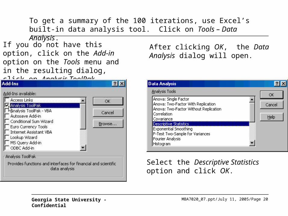
To get a summary of the 100 iterations, use Excel’s built-in data analysis tool. Click on Tools – Data Analysis.
If you do not have this option, click on the Add-in option on the Tools menu and in the resulting dialog, click on Analysis ToolPak.
After clicking OK, the Data Analysis dialog will open.
Select the Descriptive Statistics option and click OK.

MBA7020_07.ppt/July 11, 2005/Page 21Georgia State University - Confidential
In the resulting dialog, choose the Input Range (or $C$2:$C$101) to include the 100 iterations.
Now click on Output Range and enter the cell where the output will be placed.
In addition, select Summary Statistics and click OK.
MBA7020_07.ppt/July 11, 2005/Page 22Georgia State University - Confidential
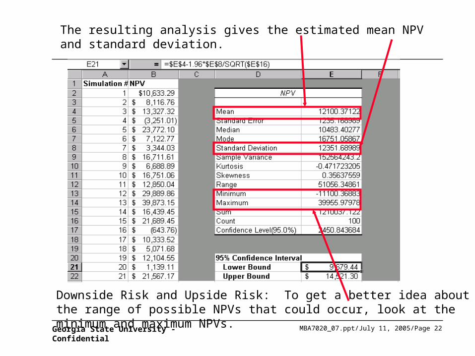
The resulting analysis gives the estimated mean NPV and standard deviation.
Downside Risk and Upside Risk: To get a better idea about the range of possible NPVs that could occur, look at the minimum and maximum NPVs.
MBA7020_07.ppt/July 11, 2005/Page 23Georgia State University - Confidential
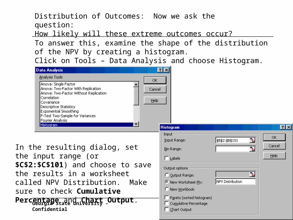
Distribution of Outcomes: Now we ask the question:How likely will these extreme outcomes occur?
To answer this, examine the shape of the distribution of the NPV by creating a histogram. Click on Tools – Data Analysis and choose Histogram.
In the resulting dialog, set the input range (or $C$2:$C$101) and choose to save the results in a worksheet called NPV Distribution. Make sure to check Cumulative Percentage and Chart Output.
MBA7020_07.ppt/July 11, 2005/Page 24Georgia State University - Confidential
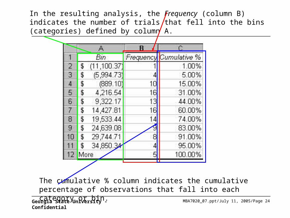
In the resulting analysis, the Frequency (column B) indicates the number of trials that fell into the bins (categories) defined by column A.
The cumulative % column indicates the cumulative percentage of observations that fall into each category or bin.

MBA7020_07.ppt/July 11, 2005/Page 25Georgia State University - Confidential
The histogram gives a visual representation of the distribution of NPVs. The histogram gives a visual representation of the distribution of NPVs. Note that it is somewhat bell shaped. Note that it is somewhat bell shaped.
MBA7020_07.ppt/July 11, 2005/Page 26Georgia State University - Confidential
How Reliable is the Simulation?
• Now the two questions about the distribution can be answered:
1. What is the mean or expected value of the NPV?In this trial, the mean is $12,100.
2. What is the probability that the NPV assumes a negative value (making the proposal to add the A3XX less attractive)?In this trial, the probability is >15%.
• The next questions to ask are:
1. How much confidence do we have in the answers from the first trial?
2. Would we be more confident if we ran more trials?
MBA7020_07.ppt/July 11, 2005/Page 27Georgia State University - Confidential
How Reliable is the Simulation?
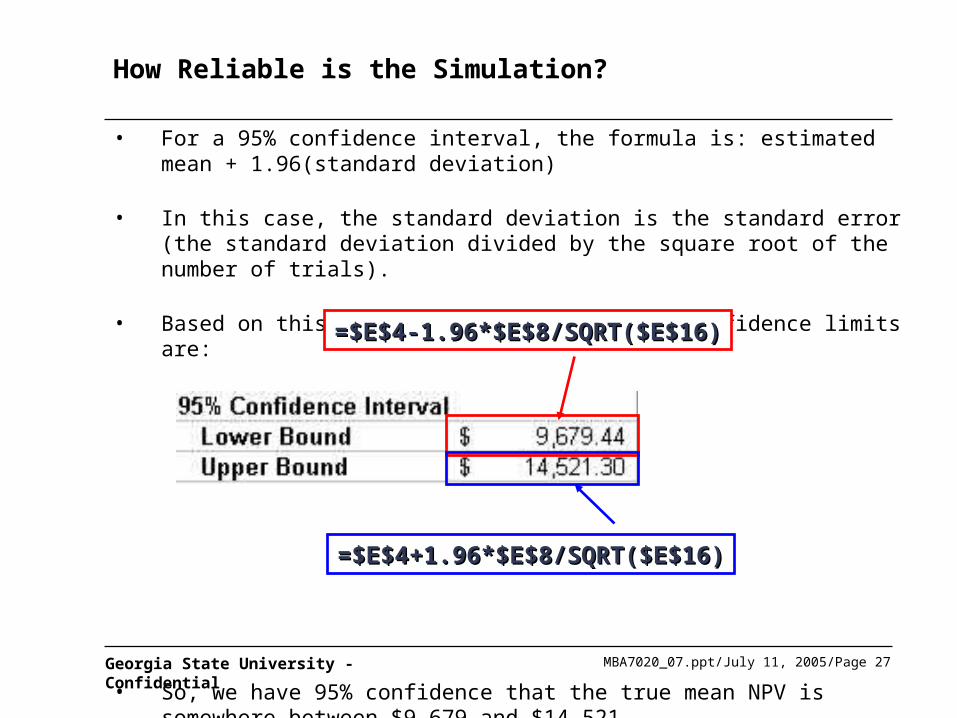
• For a 95% confidence interval, the formula is: estimated mean + 1.96(standard deviation)
• In this case, the standard deviation is the standard error (the standard deviation divided by the square root of the number of trials).
• Based on this trial, the upper and lower confidence limits are:
• So, we have 95% confidence that the true mean NPV is somewhere between $9,679 and $14,521.
=$E$4-1.96*$E$8/SQRT($E$16)=$E$4-1.96*$E$8/SQRT($E$16)
=$E$4+1.96*$E$8/SQRT($E$16)=$E$4+1.96*$E$8/SQRT($E$16)
MBA7020_07.ppt/July 11, 2005/Page 28Georgia State University - Confidential
Agenda
Simulation with Crystal
Ball
Spreadsheet Simulation
What is Simulation
MBA7020_07.ppt/July 11, 2005/Page 29Georgia State University - Confidential
Simulating with Spreadsheet Add-ins – Crystal Ball
• Spreadsheet add-ins such as Crystal Ball and @Risk simplify the process of generating random variables and assembling the statistical results.
• To illustrate, return to the capital budgeting example.
MBA7020_07.ppt/July 11, 2005/Page 30Georgia State University - Confidential
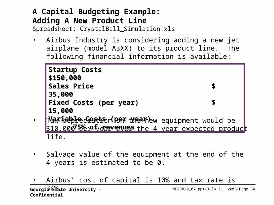
A Capital Budgeting Example: Adding A New Product LineSpreadsheet: CrystalBall_Simulation.xls
• Airbus Industry is considering adding a new jet airplane (model A3XX) to its product line. The following financial information is available:
• Tax depreciation on the new equipment would be $10,000 per year over the 4 year expected product life.
• Salvage value of the equipment at the end of the 4 years is estimated to be 0.
• Airbus’ cost of capital is 10% and tax rate is 34%.
Startup CostsStartup Costs $150,000$150,000Sales PriceSales Price $ 35,000$ 35,000Fixed Costs (per year)Fixed Costs (per year) $ 15,000$ 15,000Variable Costs (per year) 75% of revenuesVariable Costs (per year) 75% of revenues
MBA7020_07.ppt/July 11, 2005/Page 31Georgia State University - Confidential
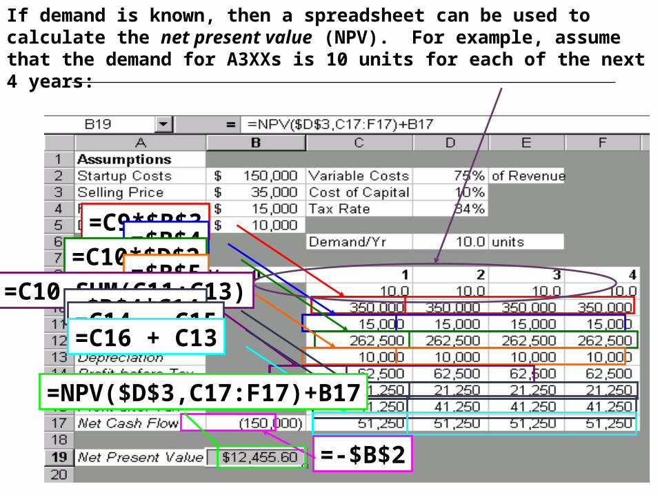
If demand is known, then a spreadsheet can be used to calculate the net present value (NPV). For example, assume that the demand for A3XXs is 10 units for each of the next 4 years:
=C9*$B$3=$B$4
=C10*$D$2=$B$5
=C10-SUM(C11:C13)=$D$4*C14=C14 – C15=C16 + C13
=-$B$2
=NPV($D$3,C17:F17)+B17
MBA7020_07.ppt/July 11, 2005/Page 32Georgia State University - Confidential
The Model with Random Demand
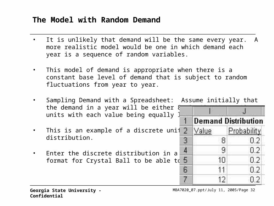
• It is unlikely that demand will be the same every year. A more realistic model would be one in which demand each year is a sequence of random variables.
• This model of demand is appropriate when there is a constant base level of demand that is subject to random fluctuations from year to year.
• Sampling Demand with a Spreadsheet: Assume initially that the demand in a year will be either 8, 9, 10, 11, or 12 units with each value being equally likely to occur.
• This is an example of a discrete uniform distribution.
• Enter the discrete distribution in a two-column format for Crystal Ball to be able to use it.
MBA7020_07.ppt/July 11, 2005/Page 33Georgia State University - Confidential
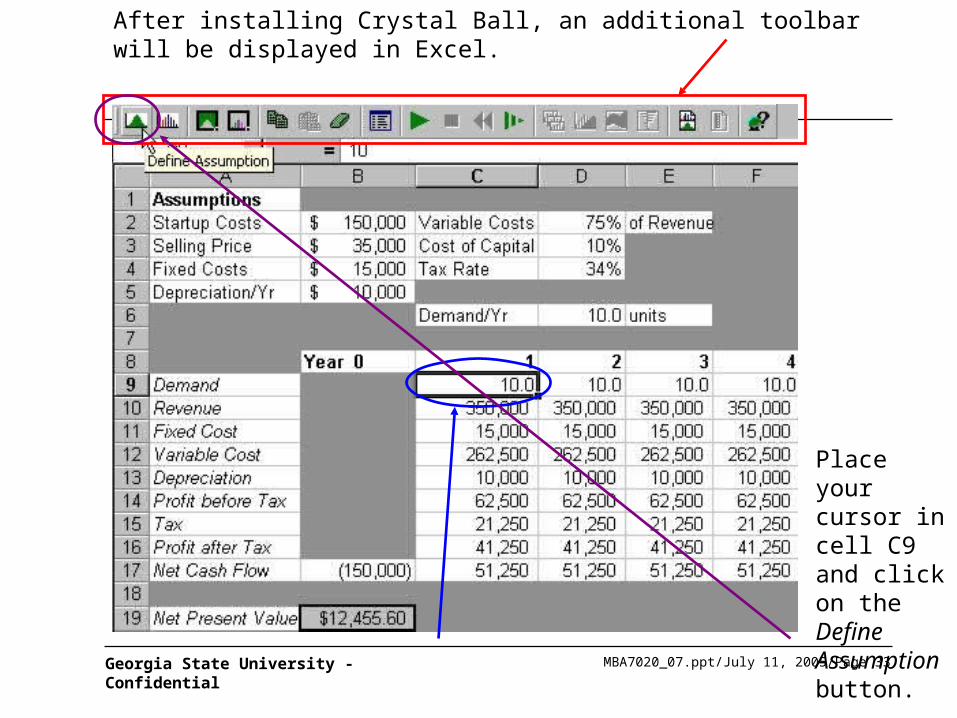
After installing Crystal Ball, an additional toolbar will be displayed in Excel.
Place your cursor in cell C9 and click on the Define Assumption button.
MBA7020_07.ppt/July 11, 2005/Page 34Georgia State University - Confidential
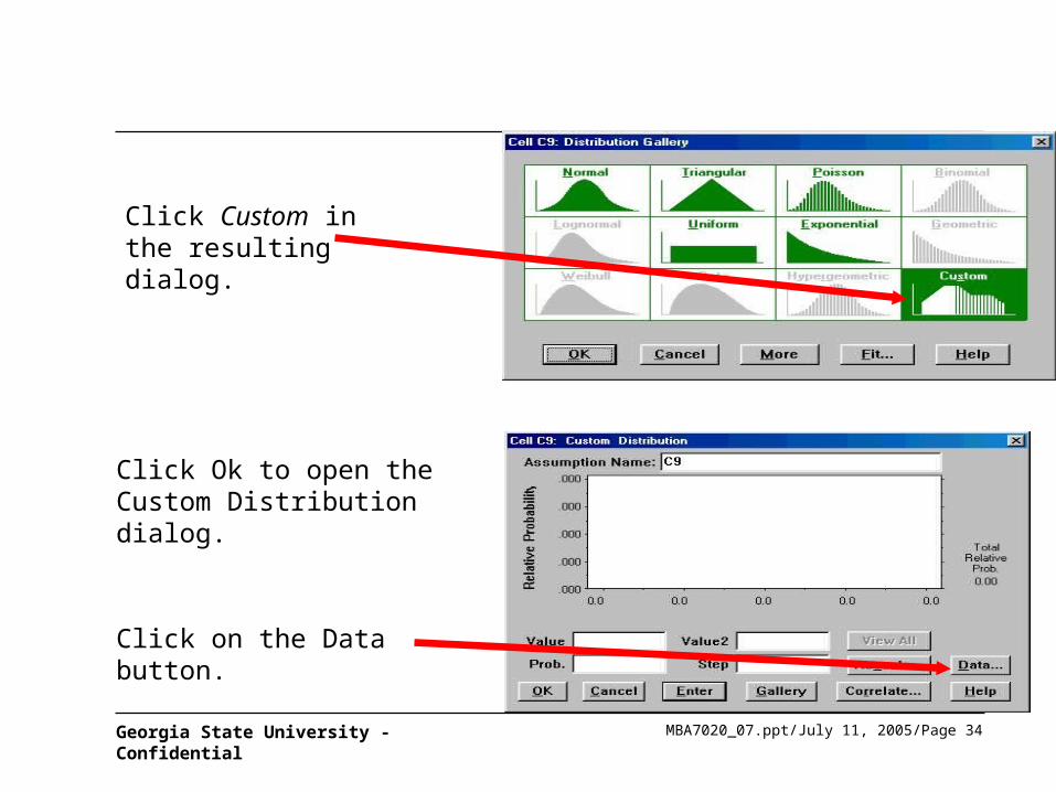
Click Custom in the resulting dialog.
Click Ok to open the Custom Distribution dialog.
Click on the Data button.
MBA7020_07.ppt/July 11, 2005/Page 35Georgia State University - Confidential
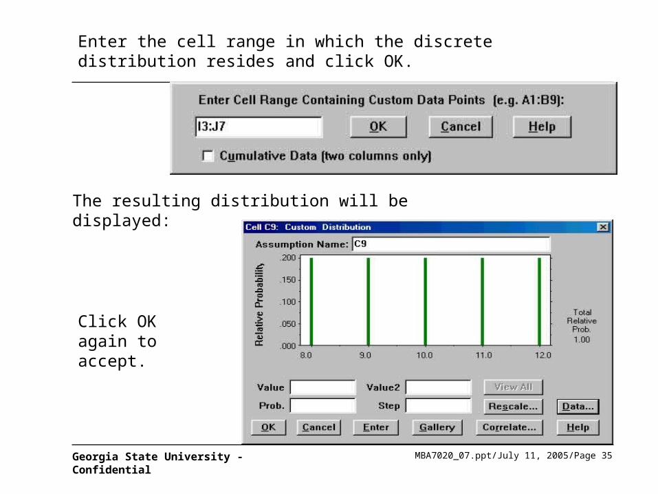
Enter the cell range in which the discrete distribution resides and click OK.
The resulting distribution will be displayed:
Click OK again to accept.
MBA7020_07.ppt/July 11, 2005/Page 36Georgia State University - Confidential
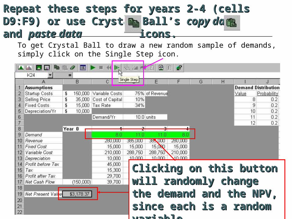
Repeat these steps for years 2-4 (cells D9:F9) or use Repeat these steps for years 2-4 (cells D9:F9) or use Crystal Ball’s Crystal Ball’s copy datacopy data and and paste datapaste data icons. icons.
To get Crystal Ball to draw a new random sample of demands, simply click on the Single Step icon.
Clicking on this button will Clicking on this button will randomly change the demand randomly change the demand and the NPV, since each is a and the NPV, since each is a random variable.random variable.
MBA7020_07.ppt/July 11, 2005/Page 37Georgia State University - Confidential
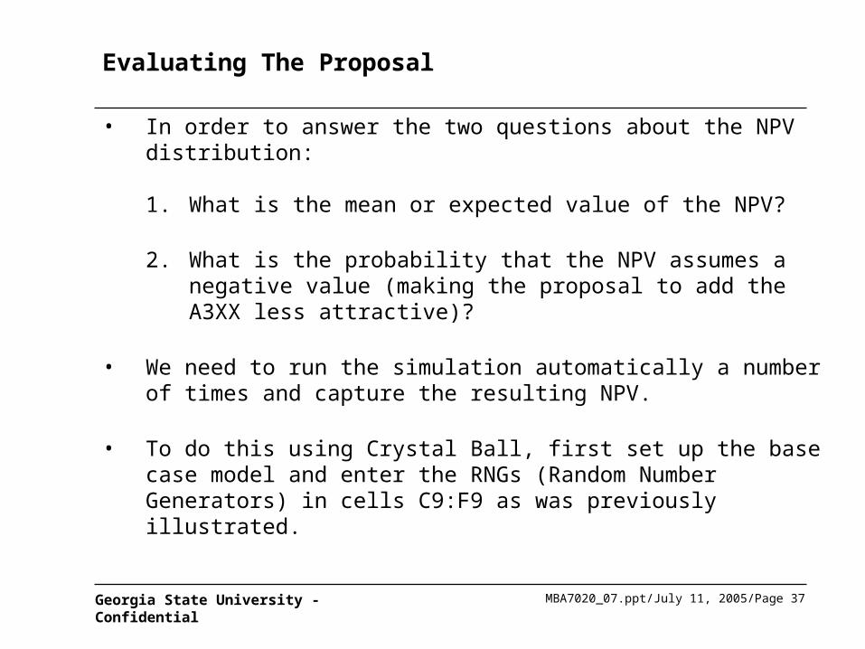
Evaluating The Proposal
• In order to answer the two questions about the NPV distribution:
1. What is the mean or expected value of the NPV?
2. What is the probability that the NPV assumes a negative value (making the proposal to add the A3XX less attractive)?
• We need to run the simulation automatically a number of times and capture the resulting NPV.
• To do this using Crystal Ball, first set up the base case model and enter the RNGs (Random Number Generators) in cells C9:F9 as was previously illustrated.
MBA7020_07.ppt/July 11, 2005/Page 38Georgia State University - Confidential
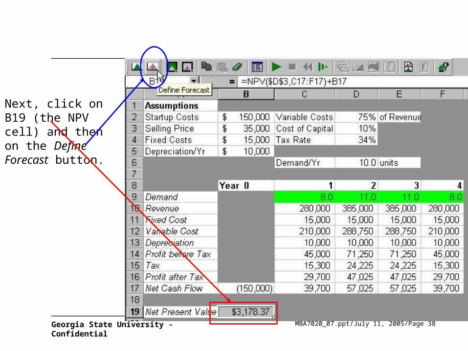
Next, click on B19 (the NPV cell) and then on the Define Forecast button.
MBA7020_07.ppt/July 11, 2005/Page 39Georgia State University - Confidential
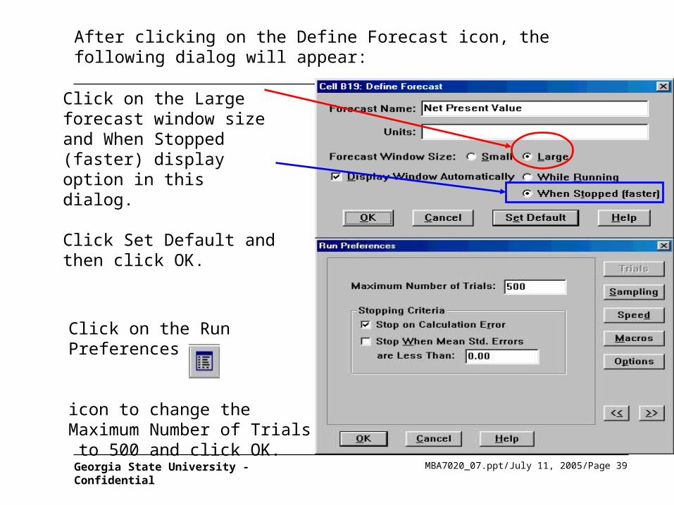
After clicking on the Define Forecast icon, the following dialog will appear:
Click on the Large forecast window size and When Stopped (faster) display option in this dialog.
Click Set Default and then click OK.
Click on the Run Preferences
icon to change the Maximum Number of Trials to 500 and click OK.
MBA7020_07.ppt/July 11, 2005/Page 40Georgia State University - Confidential
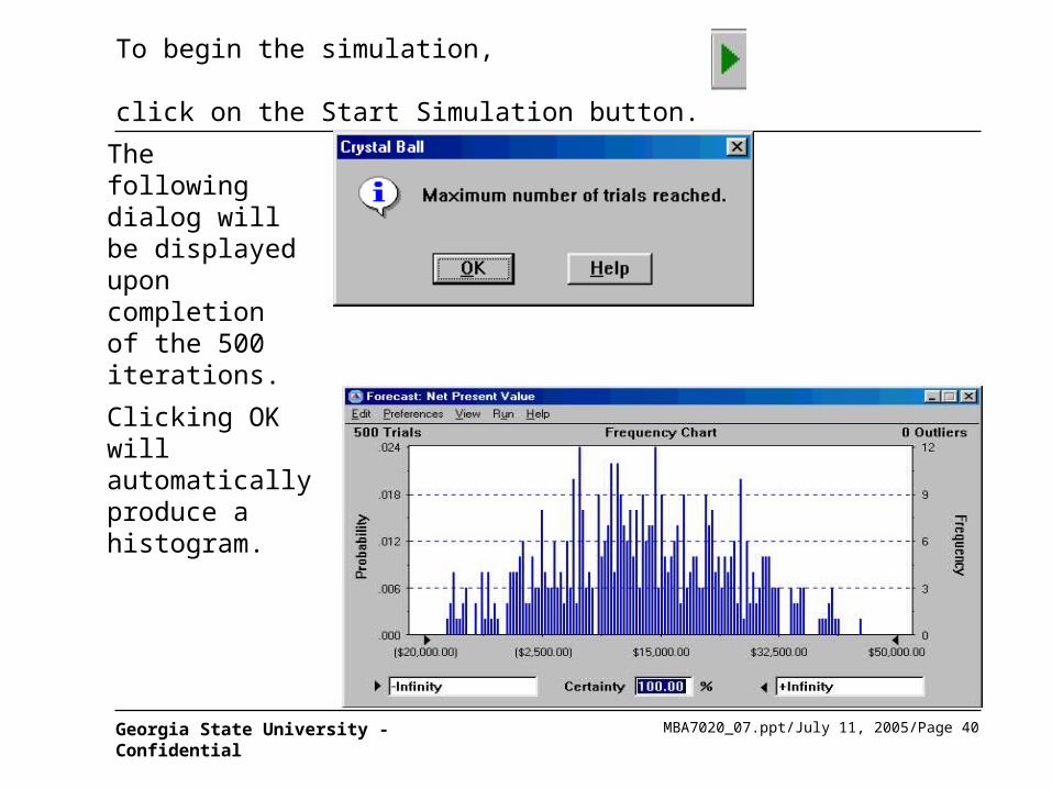
To begin the simulation,
click on the Start Simulation button.
The following dialog will be displayed upon completion of the 500 iterations.
Clicking OK will automatically produce a histogram.
MBA7020_07.ppt/July 11, 2005/Page 41Georgia State University - Confidential
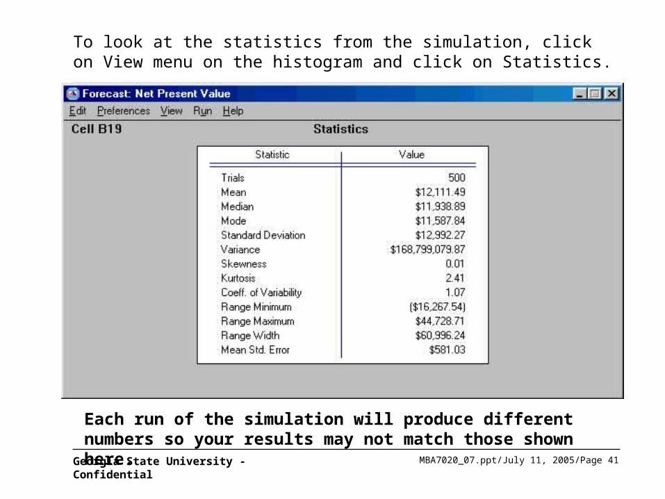
To look at the statistics from the simulation, click on View menu on the histogram and click on Statistics.
Each run of the simulation will produce different numbers so your results may not match those shown here.
MBA7020_07.ppt/July 11, 2005/Page 42Georgia State University - Confidential
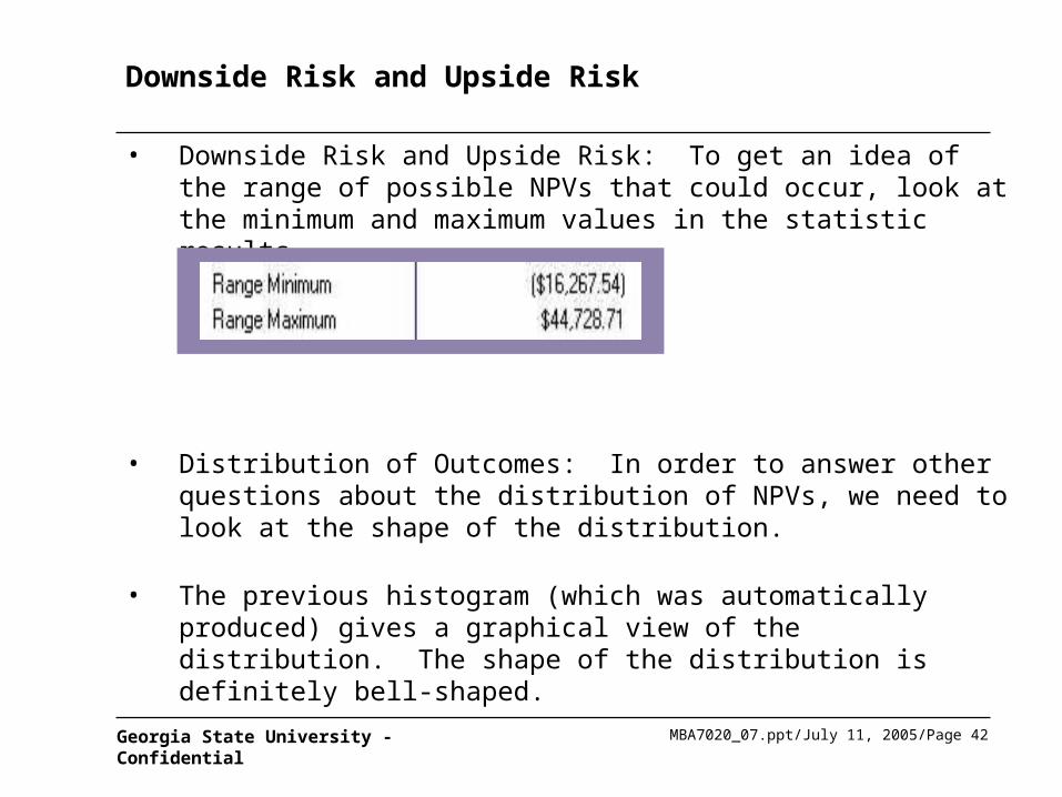
Downside Risk and Upside Risk
• Downside Risk and Upside Risk: To get an idea of the range of possible NPVs that could occur, look at the minimum and maximum values in the statistic results.
• Distribution of Outcomes: In order to answer other questions about the distribution of NPVs, we need to look at the shape of the distribution.
• The previous histogram (which was automatically produced) gives a graphical view of the distribution. The shape of the distribution is definitely bell-shaped.
MBA7020_07.ppt/July 11, 2005/Page 43Georgia State University - Confidential
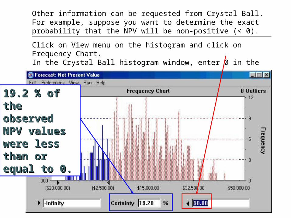
Other information can be requested from Crystal Ball. For example, suppose you want to determine the exact probability that the NPV will be non-positive (< 0).
Click on View menu on the histogram and click on Frequency Chart. In the Crystal Ball histogram window, enter 0 in the cell in the lower right
corner and hit enter.
19.2 % of the 19.2 % of the observed NPV observed NPV values were values were less than or less than or equal to 0.equal to 0.
MBA7020_07.ppt/July 11, 2005/Page 44Georgia State University - Confidential
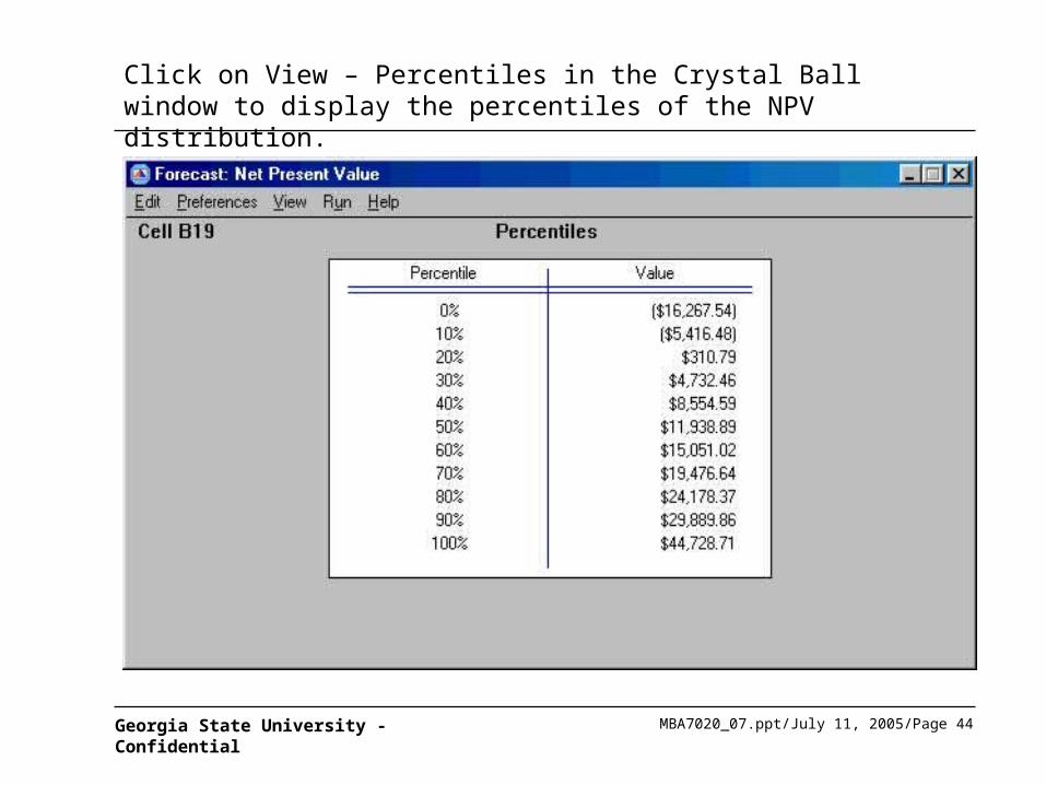
Click on View – Percentiles in the Crystal Ball window to display the percentiles of the NPV distribution.
MBA7020_07.ppt/July 11, 2005/Page 45Georgia State University - Confidential
How Reliable is the Simulation?
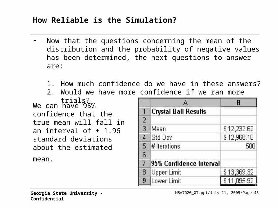
• Now that the questions concerning the mean of the distribution and the probability of negative values has been determined, the next questions to answer are:
1. How much confidence do we have in these answers?2. Would we have more confidence if we ran more trials?
We can have 95% confidence that the true mean will fall in an interval of + 1.96 standard deviations about the
estimated mean.
MBA7020_07.ppt/July 11, 2005/Page 46Georgia State University - Confidential
Other Distributions of Demand
• Originally, we started with equal mean demands of 10 for each period (year). Then, we allowed for random variation in mean demand (between 8 and 12 units). :
• Now, assume the mean demand will stay the same over the next four years, somewhere between 6 and 14 units a year, with all values being equally likely.
• This scenario can be modeled as a continuous, uniform distribution between 6 and 14.
• In addition, we can explore the impact of different demand distributions on the NPV. When the mean demand is relatively small, a distribution called the Poisson distribution is often a good fit.
MBA7020_07.ppt/July 11, 2005/Page 47Georgia State University - Confidential
Other Distributions of Demand
• The Poisson distribution is a one-parameter distribution. Specifying the mean of this distribution completely determines it.
• The Poisson distribution is a discrete distribution and the Poisson random variable can only take on non-negative integer values.
• Using Crystal Ball’s Distribution Gallery, we can easily sample from a discrete Poisson distribution or from a continuous uniform distribution.
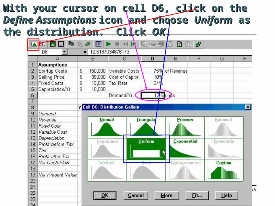
• First, indicate in Crystal Ball that the cell D6 will have the uniform distribution and that cells C9:F9 will have a Poisson distribution with a mean value driven by the value in cell D6.
MBA7020_07.ppt/July 11, 2005/Page 48Georgia State University - Confidential
With your cursor on cell D6, click on the With your cursor on cell D6, click on the Define Define Assumptions Assumptions icon and choose icon and choose UniformUniform as the as the distribution. Click distribution. Click OKOK..
MBA7020_07.ppt/July 11, 2005/Page 49Georgia State University - Confidential
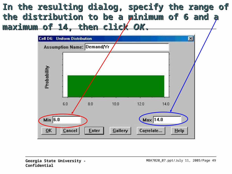
In the resulting dialog, specify the range of the In the resulting dialog, specify the range of the distribution to be a minimum of 6 and a maximum of 14, distribution to be a minimum of 6 and a maximum of 14, then click then click OKOK..
MBA7020_07.ppt/July 11, 2005/Page 50Georgia State University - Confidential
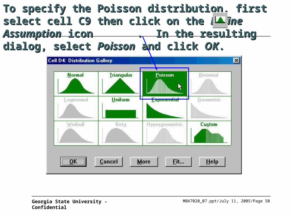
To specify the Poisson distribution, first select cell C9 To specify the Poisson distribution, first select cell C9 then click on the then click on the Define AssumptionDefine Assumption icon . In the icon . In the resulting dialog, select resulting dialog, select PoissonPoisson and click and click OKOK..
MBA7020_07.ppt/July 11, 2005/Page 51Georgia State University - Confidential
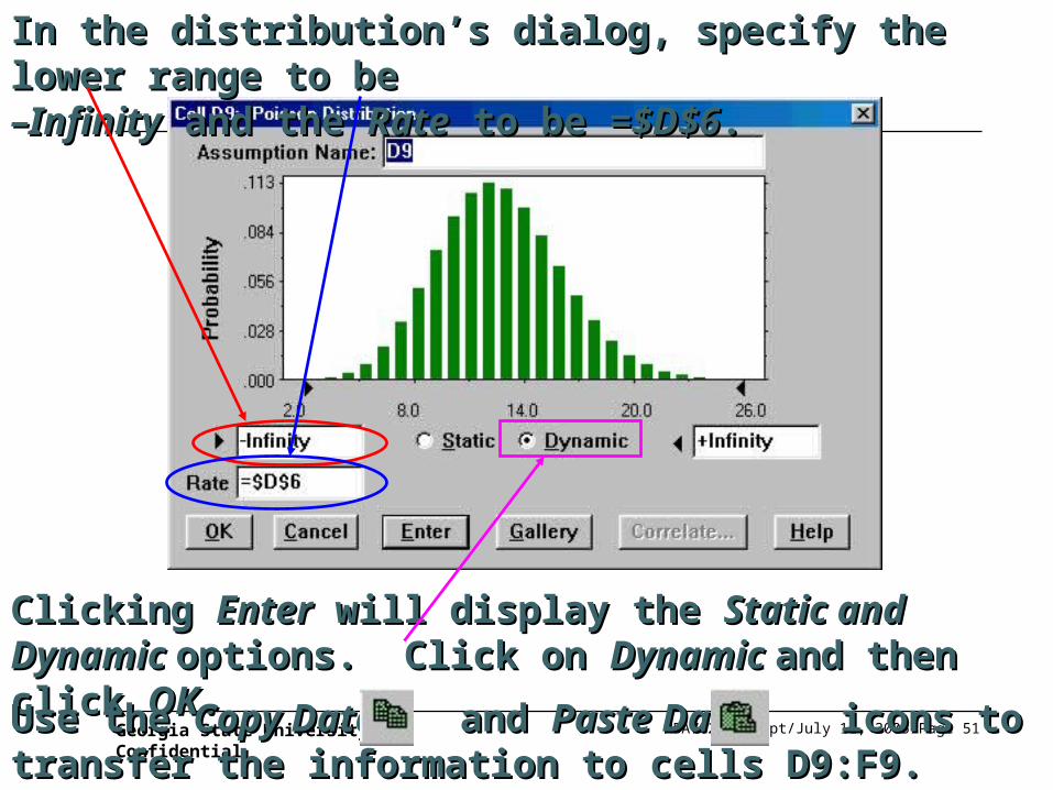
In the distribution’s dialog, specify the lower range to be In the distribution’s dialog, specify the lower range to be
–Infinity–Infinity and the and the RateRate to be to be =$D$6=$D$6. .
Clicking Clicking EnterEnter will display the will display the Static and Dynamic Static and Dynamic options. Click on options. Click on Dynamic Dynamic and then click and then click OKOK..
Use the Use the Copy Data Copy Data and and Paste Data Paste Data icons to icons to transfer the information to cells D9:F9.transfer the information to cells D9:F9.
MBA7020_07.ppt/July 11, 2005/Page 52Georgia State University - Confidential
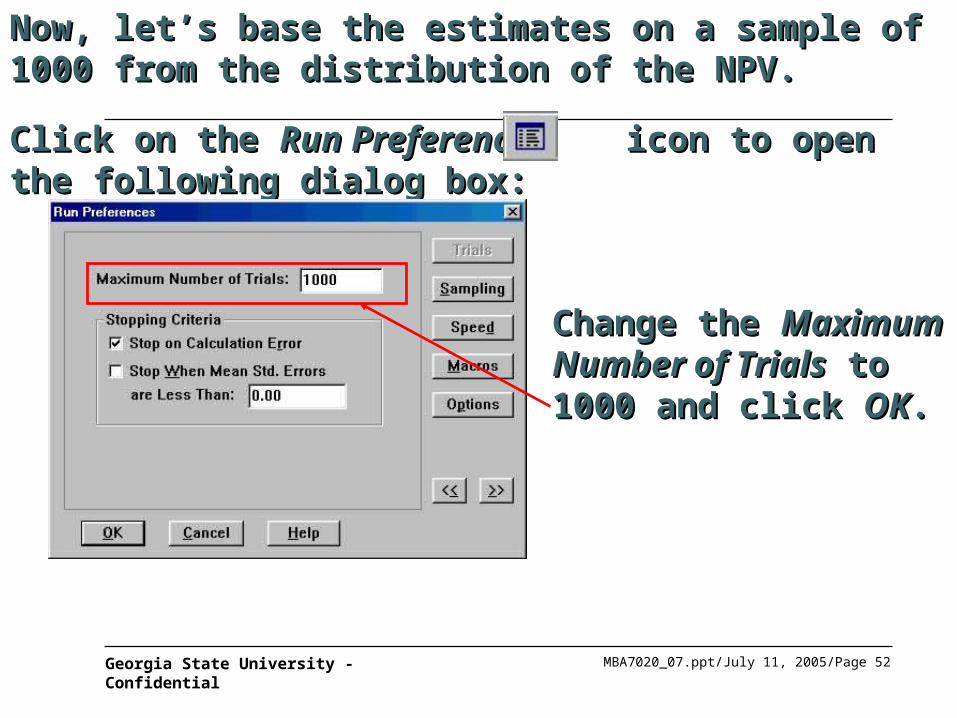
Now, let’s base the estimates on a sample of 1000 from Now, let’s base the estimates on a sample of 1000 from the distribution of the NPV.the distribution of the NPV.
Click on the Click on the Run Preferences Run Preferences icon to open the icon to open the following dialog box:following dialog box:
Change the Change the Maximum Maximum Number of TrialsNumber of Trials to to 1000 and click 1000 and click OKOK..
MBA7020_07.ppt/July 11, 2005/Page 53Georgia State University - Confidential
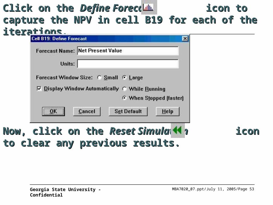
Click on the Click on the Define ForecastDefine Forecast icon to capture the icon to capture the NPV in cell B19 for each of the iterations.NPV in cell B19 for each of the iterations.
Now, click on the Now, click on the Reset SimulationReset Simulation icon to clear any icon to clear any previous results. previous results.
MBA7020_07.ppt/July 11, 2005/Page 54Georgia State University - Confidential
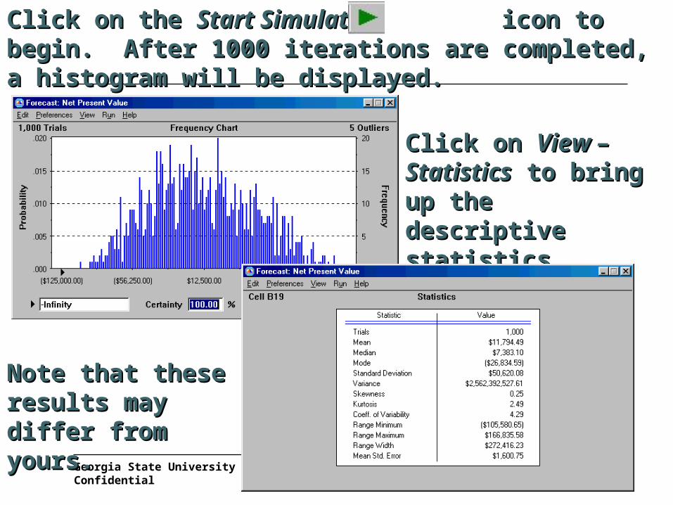
Click on the Click on the Start SimulationStart Simulation icon to begin. After icon to begin. After 1000 iterations are completed, a histogram will be 1000 iterations are completed, a histogram will be displayed.displayed.
Click on Click on View – View – StatisticsStatistics to bring up to bring up the descriptive the descriptive statistics dialog.statistics dialog.
Note that these Note that these results may differ results may differ from yours.from yours.

MBA7020_07.ppt/July 11, 2005/Page 55Georgia State University - Confidential
Based on these results, the probability of a Based on these results, the probability of a negative NPV is 44.2%.negative NPV is 44.2%.
MBA7020_07.ppt/July 11, 2005/Page 56Georgia State University - Confidential
In summary,In summary,
1.1. Increasing the number of trials is apt to give a Increasing the number of trials is apt to give a better estimate of the expected return. However, better estimate of the expected return. However, there can still be a difference between the there can still be a difference between the simulated simulated averageaverage and the true expected return. and the true expected return.
2.2. Simulations can provide useful information on the Simulations can provide useful information on the distribution results. distribution results.
3.3. Simulation results are sensitive to assumptions Simulation results are sensitive to assumptions affecting the input parameters. affecting the input parameters.


