61
MBA7020_12.ppt/July 25, 2005/Page 1 Georgia State University - Confidential MBA 7020 Business Analysis Foundations Optimization Modeling July 25, 2005
| Date post: | 03-Jan-2016 |
| Category: |
Documents |
| Upload: | dustin-oconnor |
| View: | 213 times |
| Download: | 1 times |

MBA7020_12.ppt/July 25, 2005/Page 1Georgia State University - Confidential
MBA 7020
Business Analysis Foundations
Optimization Modeling
July 25, 2005

MBA7020_12.ppt/July 25, 2005/Page 2Georgia State University - Confidential
Agenda
Sensitivity Analysis and
the Solver Add-In
Quantitative Forecasting
Models
Linear Programming
MBA7020_12.ppt/July 25, 2005/Page 3Georgia State University - Confidential
Linear Programming
• Linear programming (LP) is a method of spreadsheet optimization.
• LP is used in all type of organizations and it is used to solve an extremely wide variety of problems.
• The simplex method is a systematic, arithmetic intensive search through the set of all possible solutions for the solution that optimizes a given objective.
• We will not be using the simplex method; instead, we will learn to formulate problems as LP models.

MBA7020_12.ppt/July 25, 2005/Page 4Georgia State University - Confidential
Background Information
• The Monet Company produces four types of picture frames, which we label 1, 2, 3, and 4. The four types of frames differ in respect to size, shape, and materials used.
• Each type requires a certain amount of skilled labor, metal, and glass as shown here. The table also lists the unit selling price Monet charges for each type of frame.
Skilled Labor Metal Glass Selling Price
Frame 1 2 4 6 $28.50Frame 2 1 2 2 $12.50Frame 3 3 1 1 $29.25Frame 4 2 2 2 $21.50
MBA7020_12.ppt/July 25, 2005/Page 5Georgia State University - Confidential
Background Information -- continued
• During the coming week Monet can purchase up to 4000 hours of skilled labor, 6000 ounces of metal, and 10,000 ounces of glass.
• The unit costs are $8.00 per labor hour, $0.50 per ounce of metal and $0.75 per ounce of glass.
• Also, market constraints are such that it is impossible to sell more than 1000 type 1 frames, 2000 type 2 frames, 500 type 3 frames, and 1000 type 4 frames.
• The company wants to maximize its weekly profit.
MBA7020_12.ppt/July 25, 2005/Page 6Georgia State University - Confidential
Solution
• In the traditional algebraic solution method, we first identify the decision variables.
• In this small problem they are the number of frames of type 1, 2, 3, and 4 to produce.
• We label these x1, x2, x3, and x4.
• Next, we write total profit and the constraints in terms of x’s.
• Finally, since only nonnegative amounts can be produced, we add explicit constraints to ensure that the x’s are nonnegative.
MBA7020_12.ppt/July 25, 2005/Page 7Georgia State University - Confidential
Solution -- continued
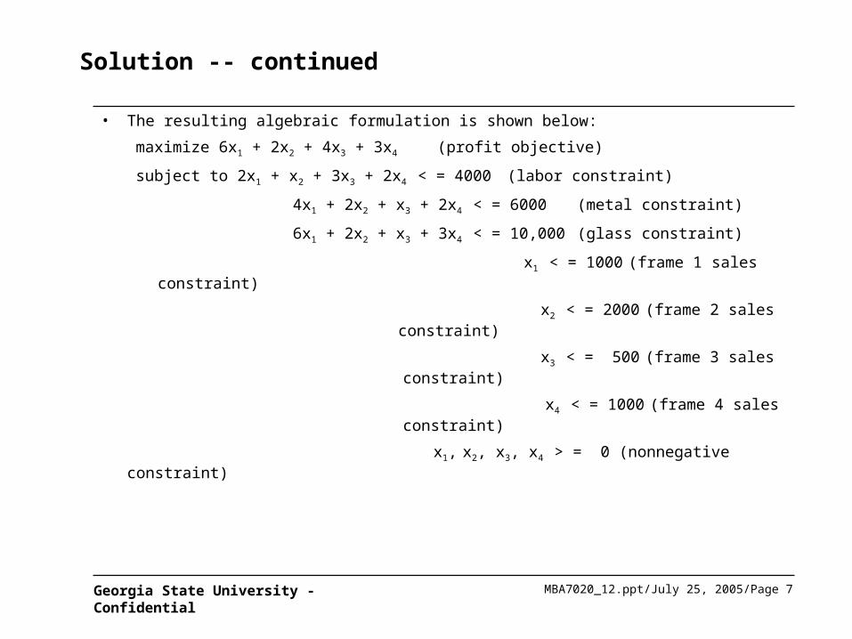
• The resulting algebraic formulation is shown below:
maximize 6x1 + 2x2 + 4x3 + 3x4 (profit objective)
subject to 2x1 + x2 + 3x3 + 2x4 < = 4000 (labor constraint)
4x1 + 2x2 + x3 + 2x4 < = 6000 (metal constraint)
6x1 + 2x2 + x3 + 3x4 < = 10,000 (glass constraint)
x1 < = 1000 (frame 1 sales constraint)
x2 < = 2000 (frame 2 sales constraint)
x3 < = 500 (frame 3 sales constraint)
x4 < = 1000 (frame 4 sales constraint)
x1, x2, x3, x4 > = 0 (nonnegative constraint)
MBA7020_12.ppt/July 25, 2005/Page 8Georgia State University - Confidential
Solution -- continued
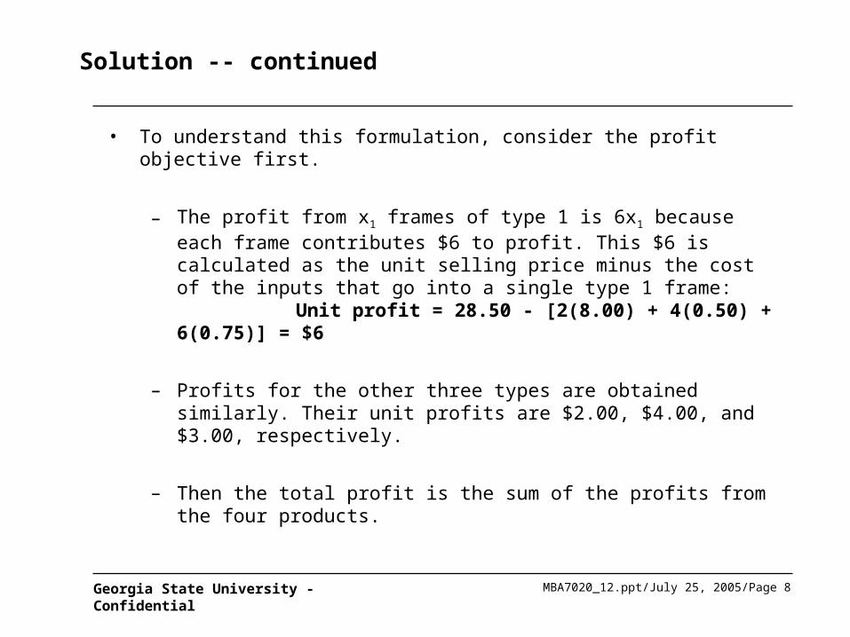
• To understand this formulation, consider the profit objective first.
– The profit from x1 frames of type 1 is 6x1 because each frame contributes $6 to profit. This $6 is calculated as the unit selling price minus the cost of the inputs that go into a single type 1 frame:
Unit profit = 28.50 - [2(8.00) + 4(0.50) + 6(0.75)] = $6
– Profits for the other three types are obtained similarly. Their unit profits are $2.00, $4.00, and $3.00, respectively.
– Then the total profit is the sum of the profits from the four products.
MBA7020_12.ppt/July 25, 2005/Page 9Georgia State University - Confidential
Solution -- continued
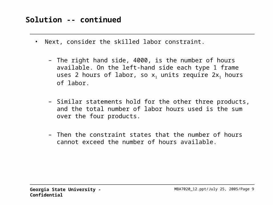
• Next, consider the skilled labor constraint.
– The right hand side, 4000, is the number of hours available. On the left-hand side each type 1 frame uses 2 hours of labor, so x1 units require 2x1 hours of labor.
– Similar statements hold for the other three products, and the total number of labor hours used is the sum over the four products.
– Then the constraint states that the number of hours cannot exceed the number of hours available.
MBA7020_12.ppt/July 25, 2005/Page 10Georgia State University - Confidential
Solution -- continued
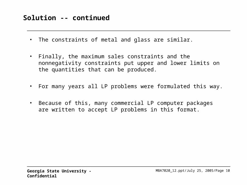
• The constraints of metal and glass are similar.
• Finally, the maximum sales constraints and the nonnegativity constraints put upper and lower limits on the quantities that can be produced.
• For many years all LP problems were formulated this way.
• Because of this, many commercial LP computer packages are written to accept LP problems in this format.
MBA7020_12.ppt/July 25, 2005/Page 11Georgia State University - Confidential
Solution -- continued
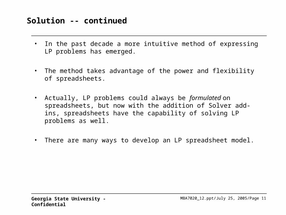
• In the past decade a more intuitive method of expressing LP problems has emerged.
• The method takes advantage of the power and flexibility of spreadsheets.
• Actually, LP problems could always be formulated on spreadsheets, but now with the addition of Solver add-ins, spreadsheets have the capability of solving LP problems as well.
• There are many ways to develop an LP spreadsheet model.
MBA7020_12.ppt/July 25, 2005/Page 12Georgia State University - Confidential
Spreadsheet Elements
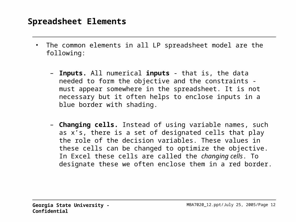
• The common elements in all LP spreadsheet model are the following:
– Inputs. All numerical inputs - that is, the data needed to form the objective and the constraints - must appear somewhere in the spreadsheet. It is not necessary but it often helps to enclose inputs in a blue border with shading.
– Changing cells. Instead of using variable names, such as x’s, there is a set of designated cells that play the role of the decision variables. These values in these cells can be changed to optimize the objective. In Excel these cells are called the changing cells. To designate these we often enclose them in a red border.
MBA7020_12.ppt/July 25, 2005/Page 13Georgia State University - Confidential
Spreadsheet Elements -- continued
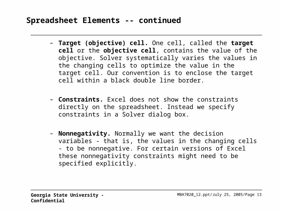
– Target (objective) cell. One cell, called the target cell or the objective cell, contains the value of the objective. Solver systematically varies the values in the changing cells to optimize the value in the target cell. Our convention is to enclose the target cell within a black double line border.
– Constraints. Excel does not show the constraints directly on the spreadsheet. Instead we specify constraints in a Solver dialog box.
– Nonnegativity. Normally we want the decision variables - that is, the values in the changing cells - to be nonnegative. For certain versions of Excel these nonnegativity constraints might need to be specified explicitly.
MBA7020_12.ppt/July 25, 2005/Page 14Georgia State University - Confidential
Solution -- continued
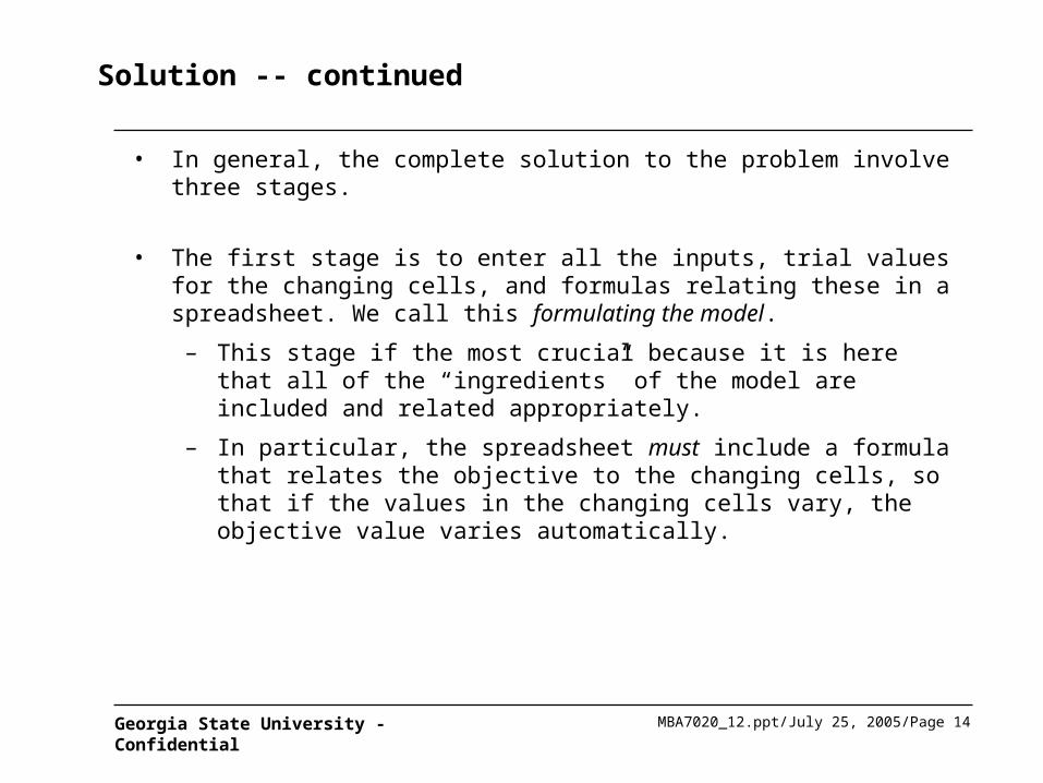
• In general, the complete solution to the problem involve three stages.
• The first stage is to enter all the inputs, trial values for the changing cells, and formulas relating these in a spreadsheet. We call this formulating the model.
– This stage if the most crucial because it is here that all of the “ingredients” of the model are included and related appropriately.
– In particular, the spreadsheet must include a formula that relates the objective to the changing cells, so that if the values in the changing cells vary, the objective value varies automatically.

MBA7020_12.ppt/July 25, 2005/Page 15Georgia State University - Confidential
Solution -- continued
• After the model is formulated, we can proceed to the second stage: invoking Solver. At this point we formally designate the objective cell, the changing cell, and the constraints, and we tell solver to find the optimal solution.
– If the first stage is done correctly, the second stage is usually very straightforward.

MBA7020_12.ppt/July 25, 2005/Page 16Georgia State University - Confidential
Solution -- continued
• The third stage is sensitivity analysis. In most model formulations of real problems, we make “best guesses” for the numerical inputs to the problem. There is typically some uncertainty about quantities such as the unit prices, forecasted demands, and resource availability.
– When we use Solver to solve he problem, we use our best estimates of these quantities to obtain an optimal solution.

MBA7020_12.ppt/July 25, 2005/Page 17Georgia State University - Confidential
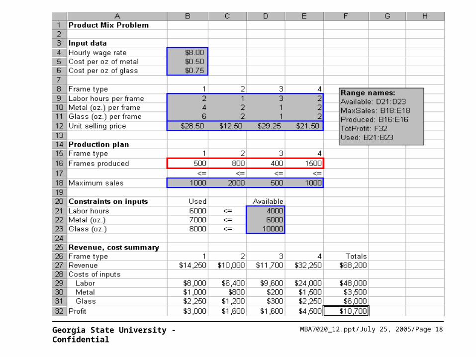
PRODUCTMIX.XLS
• This file illustrates the solution procedure for Monet’s product mix problem.
• The first stage is to set up the spreadsheet, as explained in step-by-step fashion.
MBA7020_12.ppt/July 25, 2005/Page 18Georgia State University - Confidential
MBA7020_12.ppt/July 25, 2005/Page 19Georgia State University - Confidential
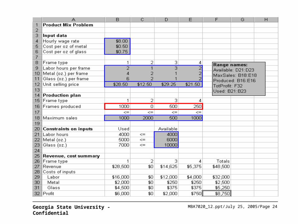
Developing the Spreadsheet Model
• Inputs. Enter the various inputs in the range B4:B6, B9:E12, B18:E18, and D21:D23.
• Production levels. Enter any four values in cells B16:E16. These do not have to be the values shown in 14.1. These cells are the changing cells; that is, the cells where the decision variables are placed. Any trail values can be used initially; Solver will eventually find the optimal values. Note that the four values shown in the initial solution cannot be optimal because they do not satisfy all of the constraints.
MBA7020_12.ppt/July 25, 2005/Page 20Georgia State University - Confidential
Developing the Spreadsheet Model -- continued
• Resources used. Enter the formula =SUMPRODUCT(B9:E9,Produced)
in cell B21 and copy it to the range B22:B23. These formulas calculate the units of labor, metal, and glass used by the current product mix. The SUMPRODUCT function is particularly helpful: it multiplies each value in the range by the corresponding value in the Products range and then sums these products.
MBA7020_12.ppt/July 25, 2005/Page 21Georgia State University - Confidential
Developing the Spreadsheet Model -- continued
• Revenues, costs and profits. The area from row 25 down shows the summary of monetary values. Actually, all we need is the total profit in cell F32, but it is useful to calculate the ingredients of this total profit (that is, the revenues and costs associated with each product). To obtain the revenues enter the formula =B12*B16 in cell B27 and copy this to the range C27:E27. For the costs, enter the formula =$B$4*B$16*B9 in cell B29 and copy this to the range B29:E21.

MBA7020_12.ppt/July 25, 2005/Page 22Georgia State University - Confidential
Developing the Spreadsheet Model -- continued
• Revenues, costs and profits - continued. Then calculate profits for each product by entering the formula =B27-SUM(B29:B31) in cell B32 and copy this to range C32:E32. Finally, calculate the totals in column F by summing across each row with the SUM function.
• The next step is to specify the changing cells, the objective cell, and the constraints in a Solver dialog box, and to instruct Solver to find the optimal solution. Before we do this, it is useful to try a few guesses in the changing cell.
MBA7020_12.ppt/July 25, 2005/Page 23Georgia State University - Confidential
Developing the Spreadsheet Model -- continued
• Trying a few guesses has two purposes.
– First, by entering different sets of values in the changing cells, we can confirm that the formulas in the other cells are working properly.
– Second, is to provide a better understanding of the model
• The resulting solution appears next.
• The corresponding profit is $8750.
MBA7020_12.ppt/July 25, 2005/Page 24Georgia State University - Confidential

MBA7020_12.ppt/July 25, 2005/Page 25Georgia State University - Confidential
Solution -- continued
• We have now produced as much as possible of the three frame type with the three highest profit margins. Does this guarantee that this solution is the best possible product? Unfortunately, it does not!
• The solution is not optimal. Even in this small model it is difficult to guess the optimal solution, even when we use a relatively intelligent trial and error procedure.
• The problem is that a frame type with a high profit margin can use up a lot of the resources and preclude other profitable frames from being produced.

MBA7020_12.ppt/July 25, 2005/Page 26Georgia State University - Confidential
Using Solver
• To invoke Excel’s Solver, select the Tools/Solver menu item. This dialog box appears.
MBA7020_12.ppt/July 25, 2005/Page 27Georgia State University - Confidential
Using Solver -- continued
• It has three important sections that you must fill in: the target cell, the changing cells, and the constraints.
• For the product mix problem, we can fill these in by typing cell references or we can point, click and drag the appropriate range in the usual way.
– Objective. Select TotProfit (cell F32) as the target cell, and click on the Maximize button.
– Changing cells. Select the Produced range (B16:E16), the numbers of frames to produce, as the changing cells.
– Constraints. Click on the Add button to add the following constraints:Used <= Available
Produced < = MaxSalesThe first constraint says to use no more of each resource than is available. The second constraint say to produce no more of each product than can be sold.
– Nonnegativity. Although negative production quantities obviously make no sense, we must tell Solver explicitly to make changing cells nonnegative. There are two ways to do this:

MBA7020_12.ppt/July 25, 2005/Page 28Georgia State University - Confidential
Using Solver -- continued
• First, we can add another constraint in Step 3:Produced >=0.
• Second, Excel 97 we can click the options button in the Solver dialog box and we can check the Assume Non-negative box in the resulting dialog box (see here).
MBA7020_12.ppt/July 25, 2005/Page 29Georgia State University - Confidential
Using Solver -- continued
– Linear model. There is one last step before clicking on the Solve button. Solvers uses one of the several numerical methods to solve various type of problems. Linear problems can be solved most efficiently by the simplex method. We must check the Assume Linear Model in the Solver options.
– Optimize. Click on the Solve button.
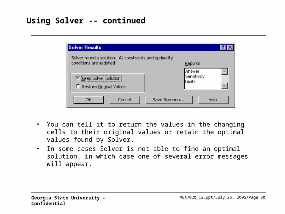
• At this point, Solver searches through a number of possible solutions until it finds the optimal solution. When it finishes it displays this message.
MBA7020_12.ppt/July 25, 2005/Page 30Georgia State University - Confidential
Using Solver -- continued
• You can tell it to return the values in the changing cells to their original values or retain the optimal values found by Solver.
• In some cases Solver is not able to find an optimal solution, in which case one of several error messages will appear.

MBA7020_12.ppt/July 25, 2005/Page 31Georgia State University - Confidential
Using Solver -- continued
• For now, clicking on the OK button to keep the Solver Solution. You should see the solutions shown on the next slide.
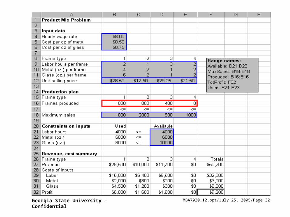
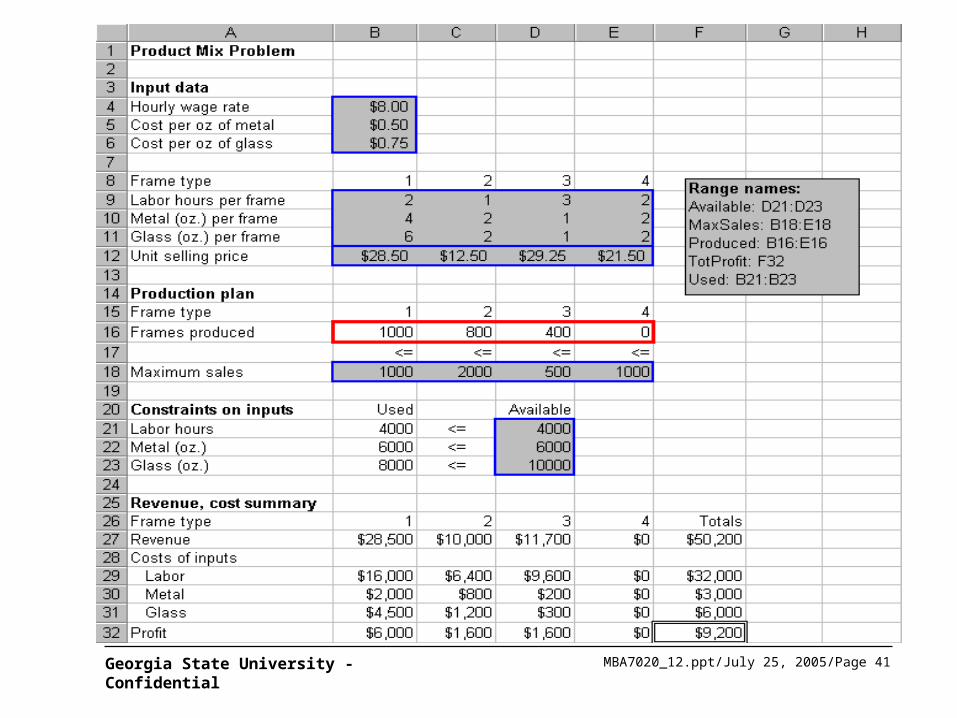
• The optimal plan is to produce 1000 type 1 frames, 800 type 2 frames, 400 type 3 frames, and no type 4 frames.
• This is close to the production plan, but the current plan earns $450 more profit.
• Also, it uses all available labor hours and metal, but only 8000 of the 10,000 ounces of glass available.
MBA7020_12.ppt/July 25, 2005/Page 32Georgia State University - Confidential

MBA7020_12.ppt/July 25, 2005/Page 33Georgia State University - Confidential
Using Solver -- continued
• Finally, in terms of maximum sales, the optimal plan could produce more of frame types 2, 3, 4 (if there were more skilled labor and/or metal available).
• This is typical of an LP solution.
• Some of the constraints are met exactly; that is, as equalities, while others contain a certain amount of “slack”.
MBA7020_12.ppt/July 25, 2005/Page 34Georgia State University - Confidential
Experimenting
• If we want to experiment with different inputs to this problem - the unit revenues or resources available, for example - we can simply change the inputs and then rerun Solver.
• As a simple what-if example, consider the modified model in the output on the next slide.
MBA7020_12.ppt/July 25, 2005/Page 35Georgia State University - Confidential
Solution to Product Mix with New Inputs
MBA7020_12.ppt/July 25, 2005/Page 36Georgia State University - Confidential
Experimenting -- continued
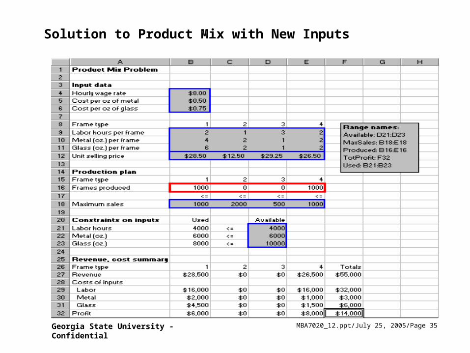
• Here the unit price for frame type 4 has increased from $21.50 to $26.50, and all other inputs have remained the same.
• By making type 4 frames more profitable, we might expect them to enter the optimal mix.
• This is exactly what happens.
• The new optimal plan discontinues production of frame type 2 and 3, and instead calls for production of 1000 units of frame type 4.
MBA7020_12.ppt/July 25, 2005/Page 37Georgia State University - Confidential
Experimenting -- continued
• There is one technical note you should be aware of.
• Because of the way the numbers are stored and calculated on a computer, the optimal values in the changing cells and elsewhere can contain small roundoff errors.
• For example for all practical purposes .000000008731 can be be treated as 0.
MBA7020_12.ppt/July 25, 2005/Page 38Georgia State University - Confidential
Agenda
Sensitivity Analysis and
the Solver Add-In
Quantitative Forecasting
Models
Linear Programming
MBA7020_12.ppt/July 25, 2005/Page 39Georgia State University - Confidential
Question
• Check how sensitive the optimal profit and the optimal product mix are to– changes in the number of labor hours available and– the cost per per ounce of metal.
• Then check how sensitive the optimal profit is to simultaneous changes in the hourly labor cost and the total labor hours available.

MBA7020_12.ppt/July 25, 2005/Page 40Georgia State University - Confidential
PRODUCTMIX.XLS
• This file illustrates the solution procedure for Monet’s product mix problem from Example 14.1.
• The product mix model has been formulated and optimized (as seen on the next slide), and the Solver/Table add-in has been installed.
MBA7020_12.ppt/July 25, 2005/Page 41Georgia State University - Confidential
MBA7020_12.ppt/July 25, 2005/Page 42Georgia State University - Confidential
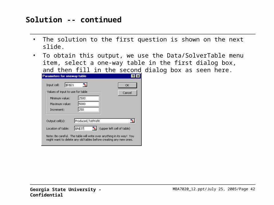
Solution -- continued
• The solution to the first question is shown on the next slide.• To obtain this output, we use the Data/SolverTable menu item, select a one-
way table in the first dialog box, and then fill in the second dialog box as seen here.
MBA7020_12.ppt/July 25, 2005/Page 43Georgia State University - Confidential
Sensitivity to available Labor Hours
MBA7020_12.ppt/July 25, 2005/Page 44Georgia State University - Confidential
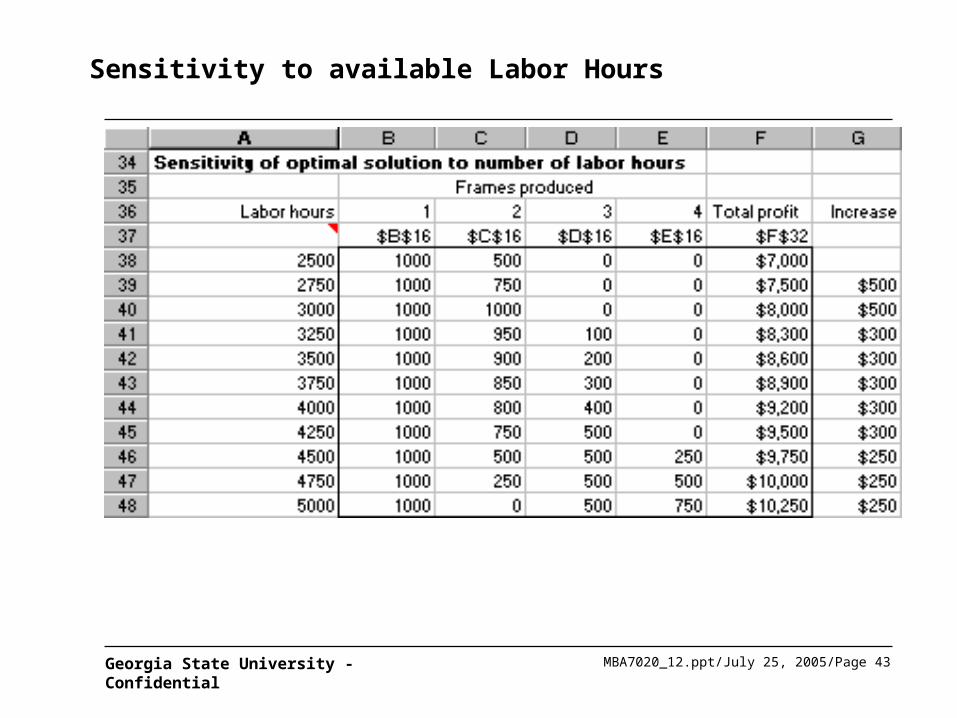
Solution -- continued
• When we click on OK, Solver solves a separate optimization problem for each of the 11 rows of the table and then reports the requested outputs in the table.
• There are several ways to interpret the output from this sensitivity analysis.
– First, we can look at columns B-E see how the product mix changes as more labor hours become available.
– Second, we can see how extra labor hours add to total profit.

MBA7020_12.ppt/July 25, 2005/Page 45Georgia State University - Confidential
Solution -- continued
• The net effect is that the labor cost increases by $2000, but this is more than offset by the increase in revenue that comes from having the extra labor hours.
• As column G illustrates, it is worthwhile to obtain extra labor hours, even though we have to pay for them, because profit increases.
• However, the increase in profit per extra labor hour, called the shadow price of labor hours, is not constant.
MBA7020_12.ppt/July 25, 2005/Page 46Georgia State University - Confidential
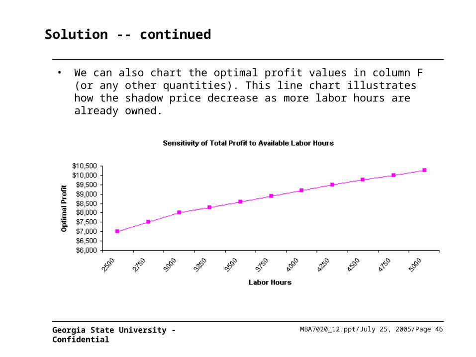
Solution -- continued
• We can also chart the optimal profit values in column F (or any other quantities). This line chart illustrates how the shadow price decrease as more labor hours are already owned.
MBA7020_12.ppt/July 25, 2005/Page 47Georgia State University - Confidential
Solution -- continued
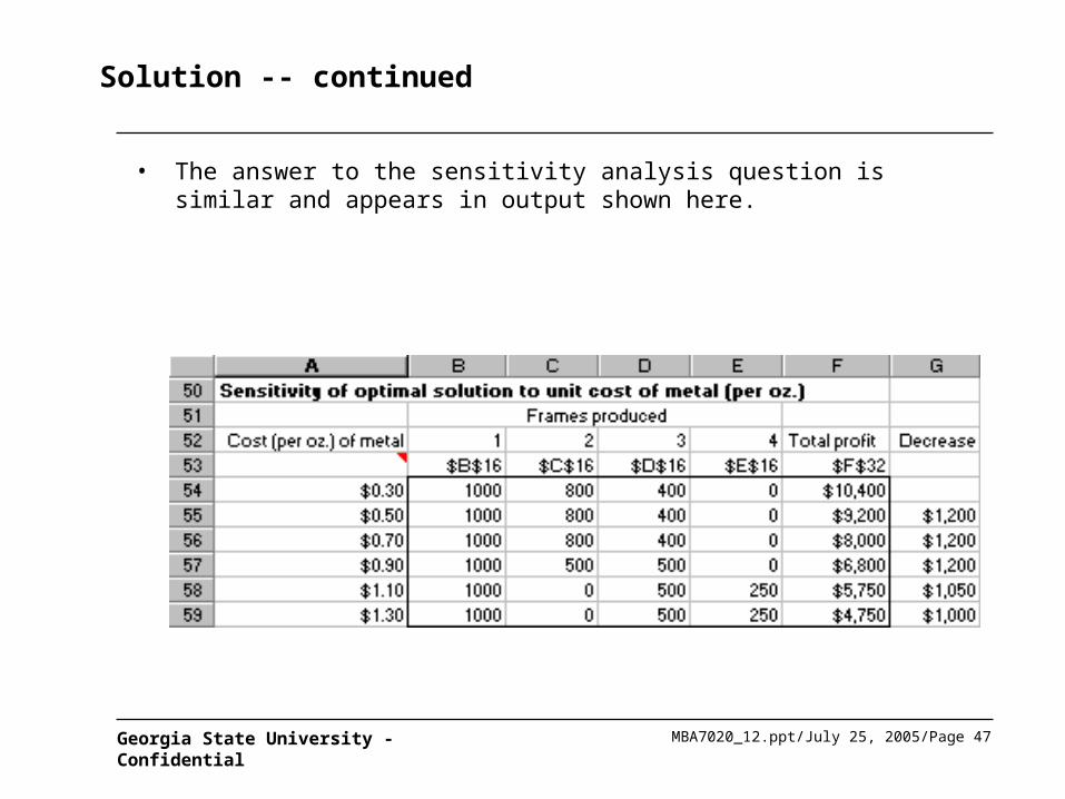
• The answer to the sensitivity analysis question is similar and appears in output shown here.
MBA7020_12.ppt/July 25, 2005/Page 48Georgia State University - Confidential
Solution -- continued
• We used Solver/Table exactly as before; only the input cell and input values differ.
• Note how the optimal product mix remains unchanged for a cost of metal in the $0.30 to $0.70 range.
• Within this range the only thing that changes is the profit.
• Intuitively, once metal becomes expensive enough, products that use metal most heavily become less attractive. They will be produced at lower levels or dropped from the mix altogether.
MBA7020_12.ppt/July 25, 2005/Page 49Georgia State University - Confidential
Solution -- continued
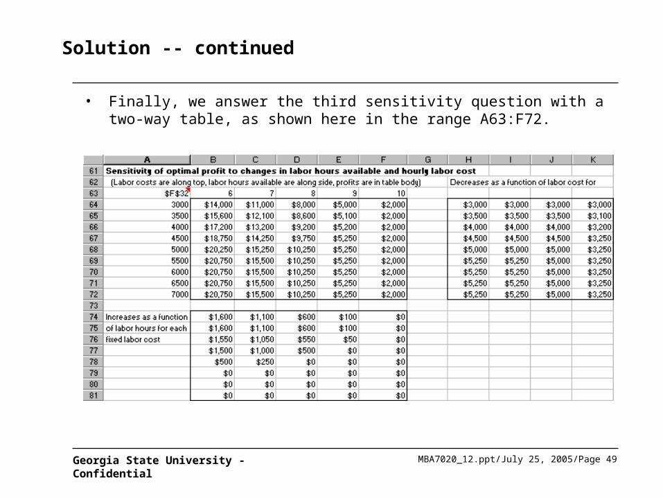
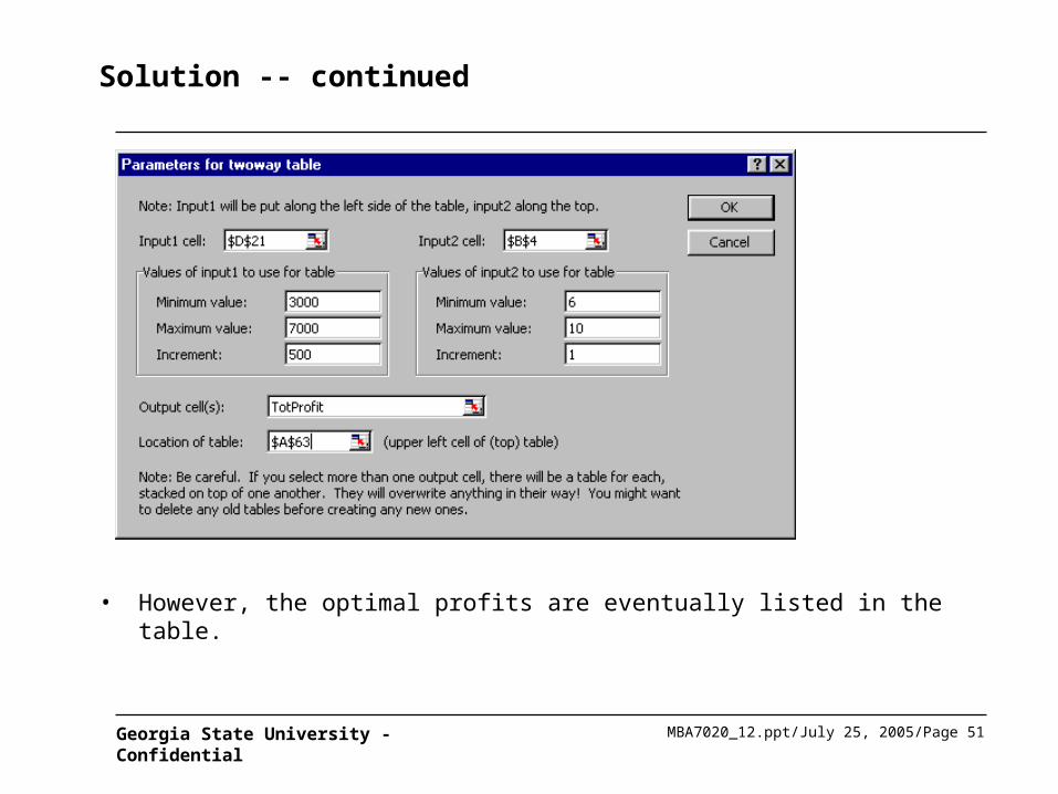
• Finally, we answer the third sensitivity question with a two-way table, as shown here in the range A63:F72.
MBA7020_12.ppt/July 25, 2005/Page 50Georgia State University - Confidential
Solution -- continued
• Now the values of the two inputs, hourly labor costs and labor hours available, are listed along the top and left-hand side, and the address of the single output, total profit, is placed in the upper left cell of the table.
• To produce this table we will complete Solver’s second dialog box as shown on the next slide.
• Now Solver must solve 45 separate problems, one for each combination of input values, so it can take up to a minute or more.
MBA7020_12.ppt/July 25, 2005/Page 51Georgia State University - Confidential
Solution -- continued
• However, the optimal profits are eventually listed in the table.
MBA7020_12.ppt/July 25, 2005/Page 52Georgia State University - Confidential
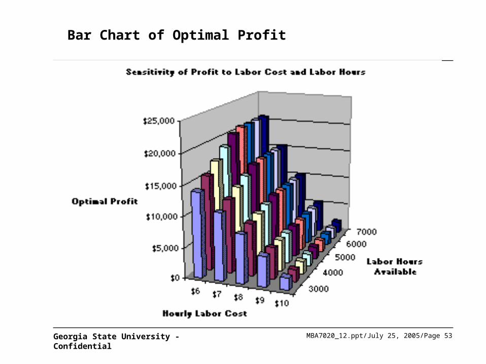
Solution -- continued
• From these, we can see how much total profit decreases in each row as the hourly labor cost increases and see how it increases in each column as the available labor hours increase.
• We also chart the profits in the table. The next slide shows one possibility.
MBA7020_12.ppt/July 25, 2005/Page 53Georgia State University - Confidential
Bar Chart of Optimal Profit
MBA7020_12.ppt/July 25, 2005/Page 54Georgia State University - Confidential
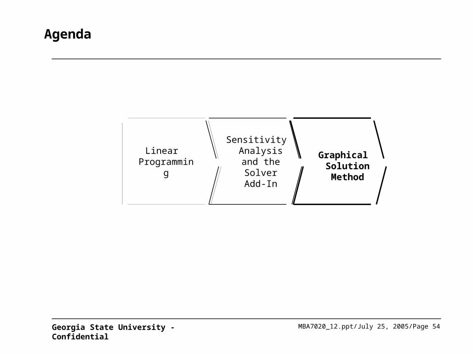
Agenda
Graphical Solution Method
Linear Programming
Sensitivity Analysis and
the Solver Add-In
MBA7020_12.ppt/July 25, 2005/Page 55Georgia State University - Confidential
Background Information
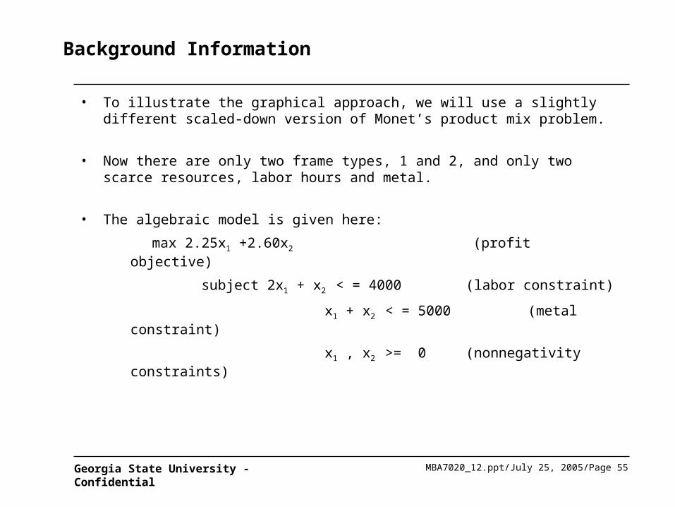
• To illustrate the graphical approach, we will use a slightly different scaled-down version of Monet’s product mix problem.
• Now there are only two frame types, 1 and 2, and only two scarce resources, labor hours and metal.
• The algebraic model is given here:
max 2.25x1 +2.60x2 (profit objective)
subject 2x1 + x2 < = 4000 (labor constraint)
x1 + x2 < = 5000 (metal constraint)
x1 , x2 >= 0 (nonnegativity constraints)

MBA7020_12.ppt/July 25, 2005/Page 56Georgia State University - Confidential
Background Information
• The objective implies that each type 1 frame contributes a profit of $2.25, whereas each type 2 frame contributes a profit of $2.60.
• The first constraint is a labor constraint.
– There are 4000 hours available. Each type 1 frame requires 2 labor hours, and each type 2 frame requires 1 labor hour.
• Similarly, the second constraint is a metal constraint.
– There are 5000 ounces of metal available. Each type 1 frame requires 1 ounce of metal, and each type 2 frame requires 2 ounces of metal.
• Find the optimal produce mix graphically.
MBA7020_12.ppt/July 25, 2005/Page 57Georgia State University - Confidential
Solution -- continued
• The idea is to graph constraints on a two-dimensional graph to see which points (x1, x2) satisfy all of the constraints.
• This set of points is labeled the feasible region. Then we see which point in the feasible region provides the largest profit.
• The graphical solution is shown on the next slide.

MBA7020_12.ppt/July 25, 2005/Page 58Georgia State University - Confidential
Graphical Solution for Monet’s Two Variable Problem
MBA7020_12.ppt/July 25, 2005/Page 59Georgia State University - Confidential
Producing the Graph
• To produce the graph, we first locate the lines where the constraints hold as equalities.
• The easiest way to graph this is to find the two points where it crosses the axes. It crosses the x1-axis when x2=0; that is, at x1=2000. Similarly it crosses the x2- axis when x1= 0; that is, at x2=4000.
• Joining these points we get the line where the labor constraint is satisfied exactly; that is, as an equality. All points below and to the left of this line are feasible; these are the points where less than the maximum of 4000 labor hours are used.
• Similarly, the metal constraint line crosses the axes at point (0,2500) and (5000,0), so we join these two points to find the line where all 5000 ounces of metal are used.
• Then all points below this line use less than 5000 ounces of metal.
• Finally, the points below both of these lines constitute the feasible region.

MBA7020_12.ppt/July 25, 2005/Page 60Georgia State University - Confidential
Producing the Graph -- continued
• The next step is to bring profit into the picture.This is done by looking at the “isoprofit” line - that is, lines where the total profit is a constant.
• Any such line can be written as 2.25x1 +2.60x2 = P where P is a constant profit level. Solving for x2 , we can determine that the isoprofit line has slope -2.25/2.60, and it crosses the vertical axis at the value P/2.60
• Graphically, we can see that the point it will touch is the point where the labor hour and metal constraint lines cross.
MBA7020_12.ppt/July 25, 2005/Page 61Georgia State University - Confidential
Producing the Graph -- continued
• We can then solve two equations and determine that x1 = 1000 and x2 = 2000, with a corresponding profit of P = $7450.
• Note that if the isoprofit lines are steep, this is because the unit price for type 1 is large relative to the unit price for frame type 2.
• If there is a large enough disparity, Monet will produce only frame type 1 and none of frame type 2. The opposite statement is true if the isoprofit lines are much less steep.
• The crucial point, however, is that only three points can be optimal: the three “corner” points in the feasible region.
• The best of these depends on the relative slopes of the constraint lines and isoprofit lines in the graph.


