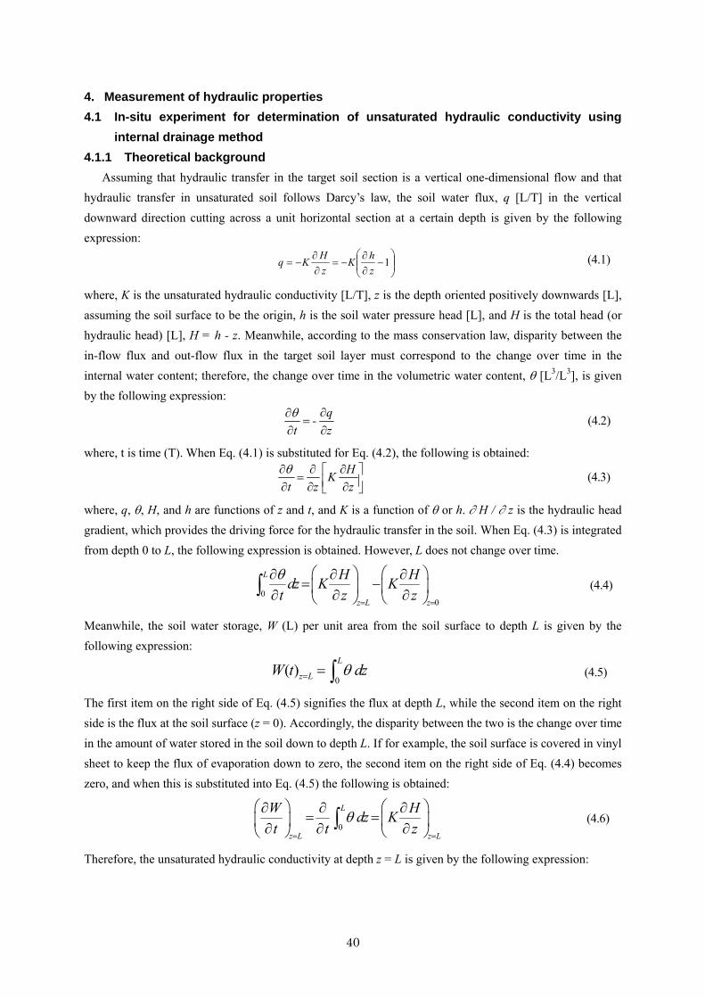
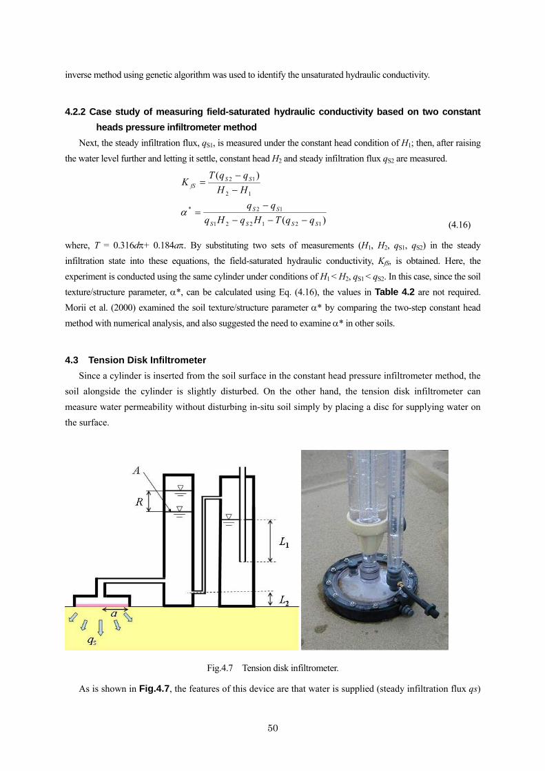
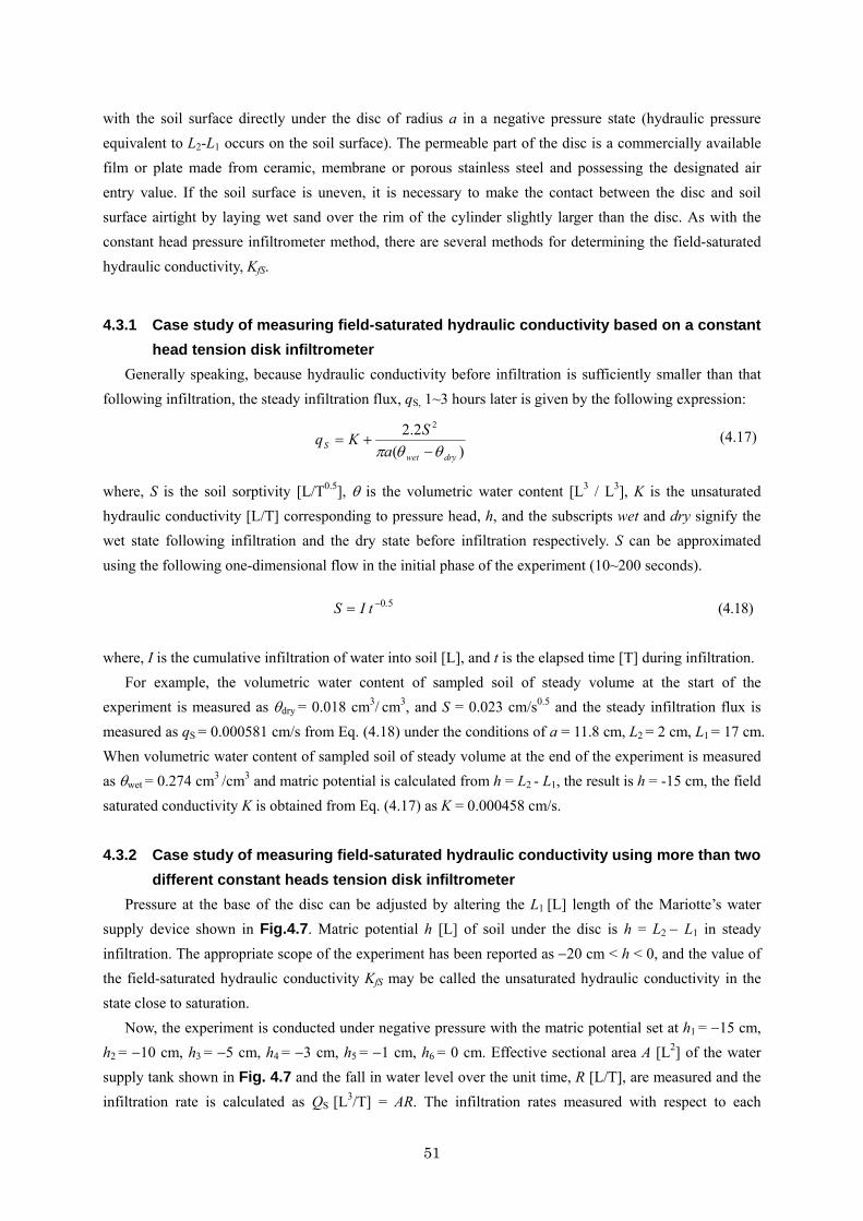
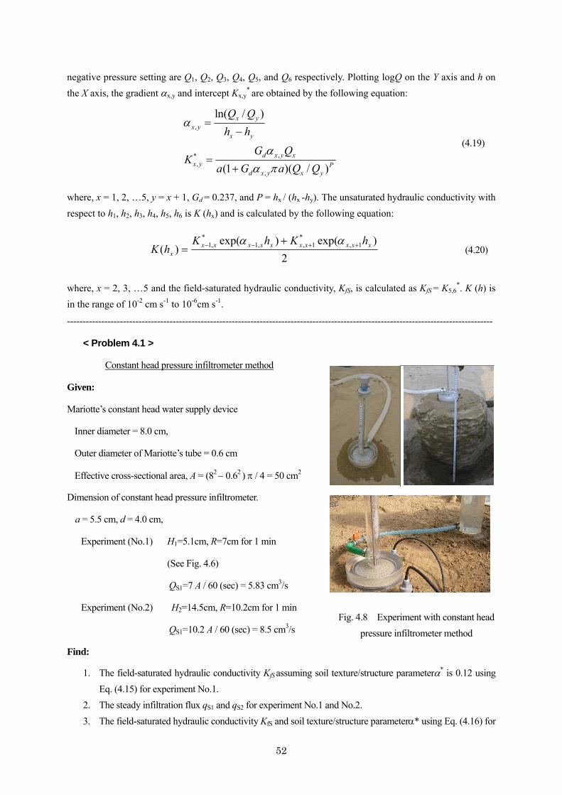
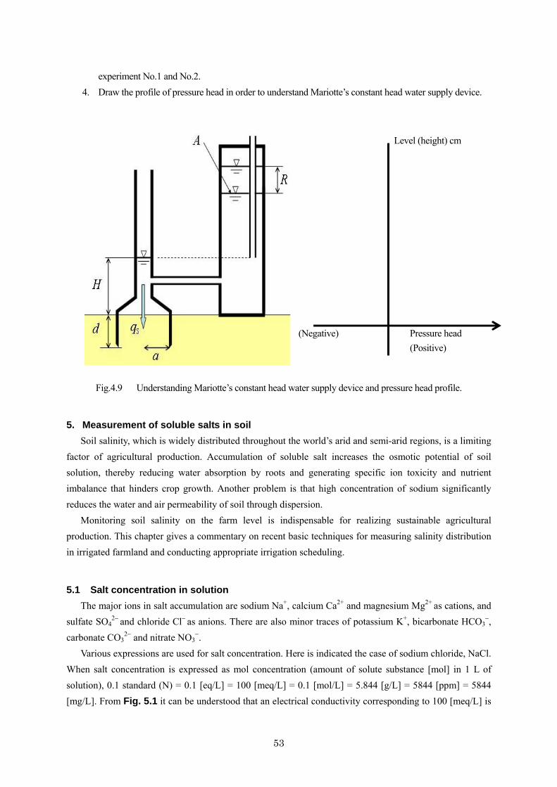
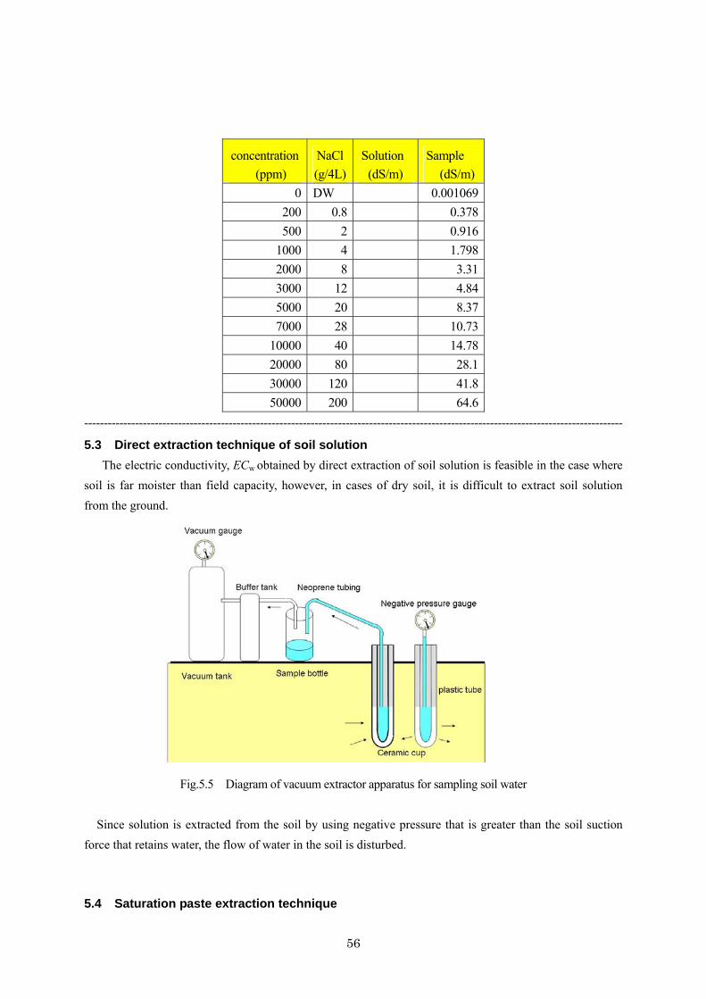
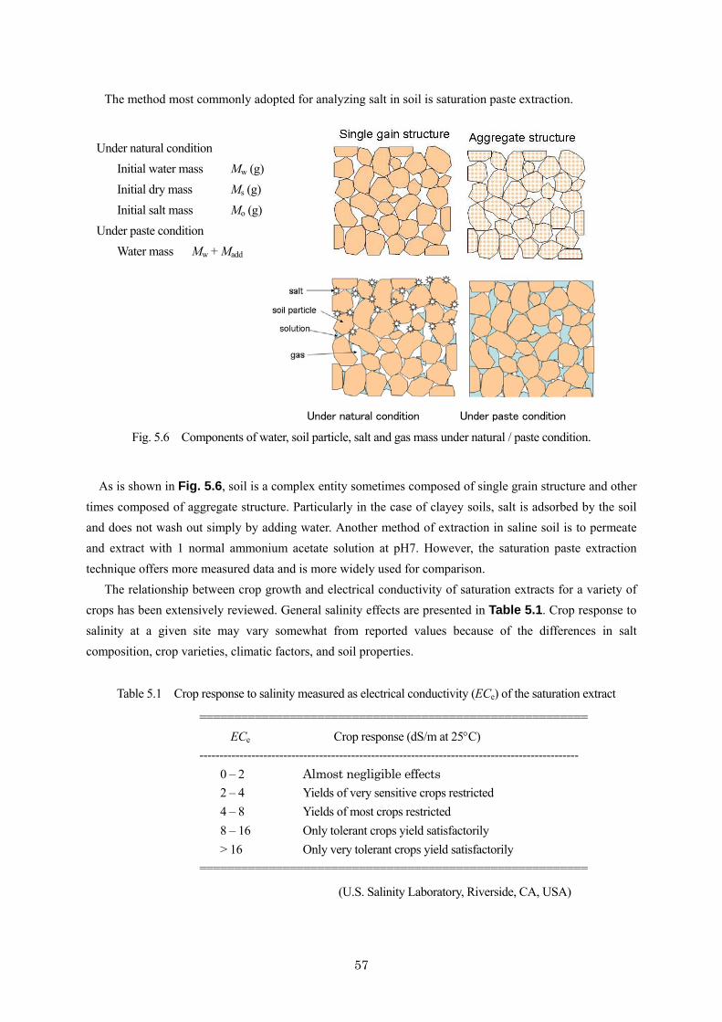
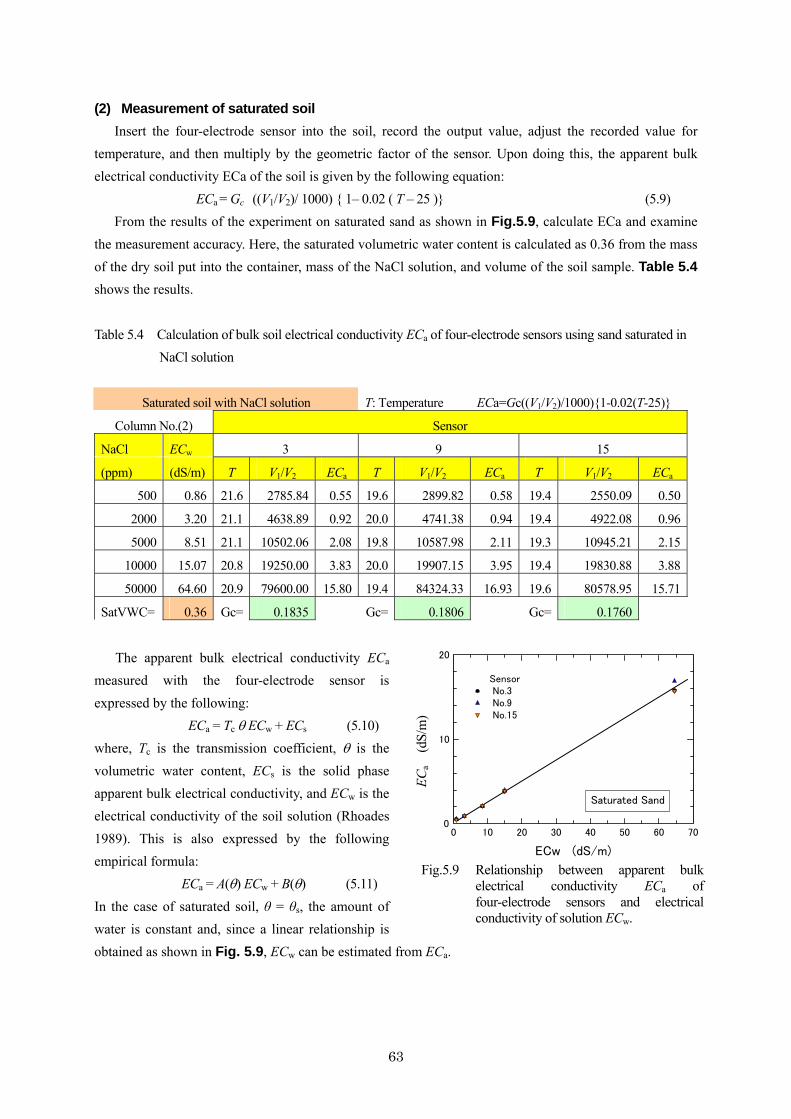
1 Management of soil physical properties Measurement of soil physical properties Dr. INOUE Mitsuhiro (Arid Land Research Center, Tottori University) 1. Introduction World population will increase to 8.6 billion in AD 2030, with approximately 85% of the population located in developing countries. With the increase in population, enough food and fibers must be secured. Attempts to achieve this have involved the deforestation and land reclamation to expand agricultural land area and the agricultural development to intensify crop production on available land. As a result, in many areas around the world, deterioration in pasture land due to over-grazing, decline in soil fertility from over-cultivation, waterlogging by over-irrigation or soil salinization due to a rise in groundwater level, may enhance soil erosion and salts accumulation in agricultural land. Thus, desertification is becoming perceptible in arid and semiarid areas. Social problems arising from the loss of agricultural land due to soil degradation have become well known. Since there is high solar radiation in arid and semiarid areas experiencing desertification, there is a potential for maximum plant photosynthesis, which is beneficial to crop production. Thus, if water resources are available through irrigation with appropriate fertilizer and salt management practices, it is possible to develop a sustainable agricultural production system. On the technology for reducing salts accumulation, there are a variety of research subjects in both wide and narrow fields, from the establishment of regional water management technology on a global scale of several hundred hectares, to the clarification of the mechanism of water flow and solute transport in unsaturated soil in columns of only a few centimeters in diameter. We take notice of the field scale studies here for the purpose of prevention of salts accumulation. When salts accumulate on soil surface in an actual field, leaching with low solute concentration water is an effective method for ensuring well-drained soils. The degree of leaching depends on the salt tolerance level of the crop at each growing stage and the relationship between concentration of soluble salts in soil solution and crops yield. It is necessary therefore to establish a soil and water management practice that will be appropriate for any specific condition. For this purpose, it is important to establish the relation between crop yield and solute concentration of soil water, as well as improving water use efficiency and soil permeability. Soil water content and electrolyte concentration of soil solution in the crop root zone need to be managed adequately. It is difficult to measure water and salt distribution in a tilled soil layer and lower layers of a field. To establish a sustainable agricultural production system, an appropriate field level management of both soil water and salt concentration in the root zone is required, making it essential to quantitatively measure the water and salt distribution both vertically and horizontally in the plow layer. In order to achieve this, there is a pressing need for the development of practical sensors that can precisely measure both water and salt content in soil under field conditions. At the same time, accurate measurement of the upward flux in soil due to evaporation from bare soil and evapotranspiration in plants, as well as the downward flux due to rainfall, irrigation, and leaching, is also required.
Transcript
1
Management of soil physical properties
Measurement of soil physical properties
Dr. INOUE Mitsuhiro
(Arid Land Research Center, Tottori University) 1. Introduction
World population will increase to 8.6 billion in AD 2030, with approximately 85% of the population located in developing countries. With the increase in population, enough food and fibers must be secured. Attempts to achieve this have involved the deforestation and land reclamation to expand agricultural land area and the agricultural development to intensify crop production on available land. As a result, in many areas around the world, deterioration in pasture land due to over-grazing, decline in soil fertility from over-cultivation, waterlogging by over-irrigation or soil salinization due to a rise in groundwater level, may enhance soil erosion and salts accumulation in agricultural land. Thus, desertification is becoming perceptible in arid and semiarid areas. Social problems arising from the loss of agricultural land due to soil degradation have become well known.
Since there is high solar radiation in arid and semiarid areas experiencing desertification, there is a potential for maximum plant photosynthesis, which is beneficial to crop production. Thus, if water resources are available through irrigation with appropriate fertilizer and salt management practices, it is possible to develop a sustainable agricultural production system. On the technology for reducing salts accumulation, there are a variety of research subjects in both wide and narrow fields, from the establishment of regional water management technology on a global scale of several hundred hectares, to the clarification of the mechanism of water flow and solute transport in unsaturated soil in columns of only a few centimeters in diameter. We take notice of the field scale studies here for the purpose of prevention of salts accumulation.
When salts accumulate on soil surface in an actual field, leaching with low solute concentration water is an effective method for ensuring well-drained soils. The degree of leaching depends on the salt tolerance level of the crop at each growing stage and the relationship between concentration of soluble salts in soil solution and crops yield. It is necessary therefore to establish a soil and water management practice that will be appropriate for any specific condition. For this purpose, it is important to establish the relation between crop yield and solute concentration of soil water, as well as improving water use efficiency and soil permeability. Soil water content and electrolyte concentration of soil solution in the crop root zone need to be managed adequately. It is difficult to measure water and salt distribution in a tilled soil layer and lower layers of a field. To establish a sustainable agricultural production system, an appropriate field level management of both soil water and salt concentration in the root zone is required, making it essential to quantitatively measure the water and salt distribution both vertically and horizontally in the plow layer. In order to achieve this, there is a pressing need for the development of practical sensors that can precisely measure both water and salt content in soil under field conditions. At the same time, accurate measurement of the upward flux in soil due to evaporation from bare soil and evapotranspiration in plants, as well as the downward flux due to rainfall, irrigation, and leaching, is also required.
2
To establish a practical system for measuring water content and salt concentration in soil, the author used an undisturbed measurement to avoid disturbing the root zone, to improve four-electrode sensors and tensiometers with pressure transducer for the simultaneous measurement of salt and water in soil. In addition, basic research was performed on the effects of salt using a dielectric soil moisture probe. While incorporating this new information, we will explain the basic theory and practice as well as measurements of soil water flow and solute transport at the field level. 2. Measurement of soil water content 2.1 Three-phase model
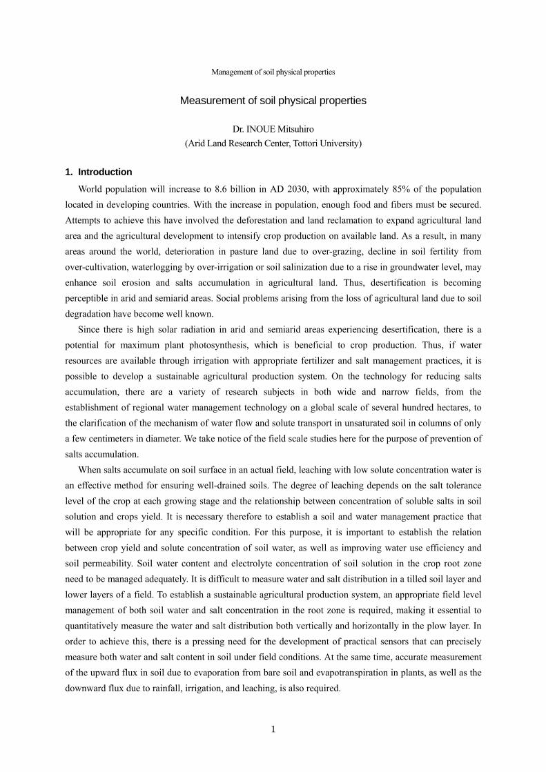
The soil is a heterogeneous entity, containing a wide range of materials such as solid particles, soil solution, gasses, vegetative roots (organic matter), small animals such as earthworms and microorganisms, and man-made materials such as nails and glasses. Therefore, when investigating the mechanics, physics, and chemistry of a soil, samples must be collected from many locations so that a statistical evaluation can be performed based on average values and standard deviation. A simplified model with three soil phases is used to collect soil samples and determine water content. (See Fig. 2.1.)
Volume components Mass components
Vt : Total bulk volume Vp : Volume of pores Va : Volume of air Vw : Volume of water Vs : Volume of solids Mw : Mass of water Ms : Mass of solid Mt : Total bulk mass
Fig. 2.1 Schematic diagram of the soil as a three-phase system.
Soils are made up of three phases: a solid phase (s), liquid phase (w), and gaseous phase (a). If the mass
of each is defined as Ms, Mw, and Ma, the volume of each is defined as Vs, Vw, and Va, the total volume of all samples is defined as Vt, and the total mass of all samples is defined as Mt, the basic index for water content in soil is expressed as:
Water content mass ratio: w = Mw /Ms
Volumetric water content: θ = Vw / Vt (2.1) Degree of saturation Sr = Vw / (Vw + Va)
In addition, dry bulk density ρd is the mass of the solid phase divided by the total volume of soil samples, and can be expressed as: ρd = Ms / Vt.
Wet bulk density ρt is the mass of total soil divided by the total volume of samples, and can be expressed as: ρt = Mt / Vt.
Relationship between volumetric water content and water content: θ = w ρd / ρw
Va
Vt
Air
Water Vp
Mw Vw
Vs
Mt
Solid Ms
Soil particle
Soil water
Air
3
Relationship between volumetric water content and saturation ratio: θ = φ Sr (2.2) where, φ is porosity defined as φ = Vp / Vt =1 - (ρ d / ρ s). ρw is the density of water, and ρ s is soil particle density, with ρ s= Ms / Vs. 2.2 Core soil sampling techniques
The core soil sampling technique is performed so that uniform sample volumes are obtained. Although sampling may be undisturbed or disturbed, the volumetric water content and dry density for undisturbed soil can be determined by sampling at a constant volume. The variation in the values of volumetric water content and dry density is dependent upon the sample size. In general, the measured variation will be larger as the sample size is smaller. In addition, variation will increase even for the same sample size as the aggregate structure develops, clay content increases, and the soil volume is subject to shrinkage and swelling. It is necessary to use the minimum sample volume where physical and chemical properties are uniform within the target region, and consider a representative sample size to determine the size of the core soil sample.
In a laboratory experiment, for example, take 100cm3 of undisturbed sample with the core soil sampler and use it for soil water retention test and unsaturated hydraulic conductivity test, using the suction method and the multi-step outflow method. For the soil column method of water retention test, for example, pile up transparent acrylic cylinders with an inner diameter of 50mm, an outer diameter of 60mm, and a height of 20mm, and fill soil into the cylinders uniformly. Place this column perpendicularly on a water surface, and when the distribution of the internal soil water reaches an equilibrium, take soil samples in rings starting from the top to find the water content. This method can be applied to disturbed core soil samples to simultaneously determine volumetric water content and dry bulk density.
Unlike the core soil sampling technique, a device called a stick-type soil sampler, for example, is used in-situ to sample soil from a deep layer, and the gravimetric method is used to determine the water content. If the dry bulk density is already known, you can multiply the water content mass ratio by the dry bulk density to determine the volumetric water content. When using a manual stick-type soil sampler to sample soil on-site, the depth limit is approximately 2 meters.
Problems with the core soil sampling technique include: (1) Since the gravimetric method is based on mass measurements, the container mass Mv is measured. As measurements are made before (Ms+Mw+Mv) and after drying (Ms+Mv), instrument error occurs when measuring with an electronic balance; (2) For a soil containing hygroscopic water, like heavy clays, soil moisture cannot be completely removed with 105°C dry heat; (3) Approximately 12 to 24 hours is required to get soil dried; (4) When measuring soil samples on-site, undisturbed soil may become disturbed, and errors may occur during conveyance; (5) Although the soil sampling technique is used to directly measure water content in soil, the site is disturbed by the collection of a large number of samples, making this technique ill-suited for continued measurements; (6) Regular sampling requires a lot of time and labor. However, this technique is simple and necessary for calibration tests that use indirect techniques, such as the electric resistance method and dielectric constant method described in Example 2.2.
For in-situ testing, earth boring equipment is used to open a hole to a specified depth, to sample undisturbed core samples at the lower horizon. Boring equipment that can be mounted on the rear of a passenger truck can be used for cylindrical sampling with an internal diameter of 80mm and a height of
4
60mm, while motorized soil sampling equipment mounted on tractors or Caterpillars can take samples with an internal diameter of 50, 80, or 100mm and length of 250mm, for continuous soil sampling to a maximum depth of 5m (for 50mm diameter). Although core samplers with volumes of 50 to 2000cm3 are commercially available, there is no global standard. When cylindrical samples with an inner diameter from 200mm to 600mm are used, major work operations are needed. Blades are mounted at the bottom of the cylinder, perpendicular to the surface of the earth. Shovels are used to dig around the periphery of the cylinder as it is pushed into the ground. At the bottom, a horizontal board is pressed down by a hydraulic pump, and the top and bottom of the cylinder are supported by horizontal boards, which are fixed into place by bolts. For example, an undisturbed soil sample with an inner diameter of 590mm and a length of 1670mm is taken to use as a monolithic lysimeter for water retention, permeability, and percolation tests. One problem with sampling is that the degree of difficulty for a soil sampling differs according to the type of soil and its water content. For example, it is very difficult to use the normal auger with extremely dry sand or very moist mud, and therefore special augers are available for these kinds of samplings.
The following three methods are used to dry soil after sampling: (1) Gravimetric method: The soil sample is normally dried in an oven at 105°C for 24 to 48 hours, and then the difference in mass before and after drying (using a weighing method precise to 0.01g for a 100cm3 sampling cylinder) is divided by the volume of the container to determine the volumetric water content. (2) Microwave oven drying method: This method was devised to reduce drying time. Using a kitchen microwave oven, approximately 10g of sample can be dried in 10 to 20 minutes. Since microwaves heat the sample from inside, it is difficult to adjust temperature and the sample may be lost due to the kinds of soil aggregates or minerals. (3) Vacuum-freeze drying method: For organic soil, such as peat soil, which contains a large amount of undegraded vegetative organic matter, this organic matter may burn when using the gravimetric or microwave oven drying methods. The vacuum-freeze drying method for removing moisture without heating the sample allows drying with minimal change to the solid phase.
< Example 2.1 > Given:
A sampling cylinder has an inside diameter of 5.0 cm and height of 5.1 cm. A soil sample taken at 15 cm depth is weighed. Total mass of soil sample plus cylinder with saucer, Wa is 210.82g. After drying, the total mass of dry soil sample plus the cylinder with saucer, Wb is 174.71g. Mass of the cylinder with saucer, Wc is 91.91g. Assume the density of water ρw is 1.0 g/cm3 and the soil particle density ρs is 2.60 g/cm3.
Find: 1. Dimension of the sample cylinder by the micrometer. 2. Total volume of core sample, Vt 3. Void ratio e = Vp / Vs , soil porosity φ 4. Relative saturation S = Vw / Vp
Solution: 1. With an inside diameter of 5.0 cm and height of 5.1 cm, the total volume of the core sample is:
Vt = 3.14 ∗ 5.02 ∗ 5.1 / 4 = 100.0 cm3 2. In order to determine the void ratio e, volume of solids Vs and volume of pores Vp are obtained thus:
5
Vs = Ms / ρs = 82.80 / 2.60 = 31.85 cm3 Vp = Vt − Vs = 100 − 31.85 = 68.15 cm3
3. e = Vp / Vs = 68.15 / 31.85 = 2.14, also e = (ρ s / ρ d ) − 1 = ( 2.60 / 0.828 ) − 1 = 2.14 Soil porosity φ is φ = Vp / Vt = 68.15 / 100 = 0.68,
also, φ = 1 − ( ρ d / ρ s ) = 1 − ( 0.828 / 2.60 ) = 0.68 4. Relative saturation is calculated as S = Vw / Vp = θ Vt / Vp =36.10 / 68.15 = 0.53
2.3 Neutron scattering method
This method utilizes the following phenomenon: when a fast neutron collides with a hydrogen atom H, its speed is reduced and it becomes a thermal neutron. It is made up of a probe that uses a radioactive source (241Am-Be, for example) that emits fast neutrons and detectors (BF3 tubes, for example) to monitor thermal neutrons. In the soil, there are neutron-absorbing elements such as carbon, cadmium, boron, chlorine, and lithium that reduce the counts of the neutron moisture meter, resulting in an underestimation of water content. On the other hand, large amounts of hydrogen in forms other than H2O, such as CH3
-, NH3
-, and OH-, will result in an overestimation of water content. In addition, even in soil of the same chemical structure, the counts will increase with an increase in dry bulk density, and also with an increase in rock content. Therefore, it is necessary to perform specific calibration test on each type of soil. In addition, since the energy of the radiation source decreases according to the half-life of the specific material, it is necessary to divide the counts for the target sample by the counts for the standard device to determine the count ratio (CR), and apply it to the volumetric water content to perform a calibration test. Generally, the calibration formula is expressed as:
θ = a CR + b (2.3) Here, a and b are fitting parameters. If there is a large amount of water, or hydrogen atoms H, in the soil, there will be a large number of thermal neutrons, resulting in an increased count ratio. Therefore, the volumetric water content (θ) will increase according to the increase in the count ratio (CR). On the other hand, the range of measurement influence depends upon the water content. Now, the range of influence is defined as a sphere, with radius R.
3115θ
=R (2.4)
This is known as the van Bavel formula. As shown in Fig. 2.2, there are two types of neutron moisture meters: a depth-type neutron moisture meter and a surface-type neutron moisture meter. If a depth-type neutron moisture meter is used in an in-situ experiment, it is necessary to lay an access tube in advance, as shown in Fig. 2.2(a). For the access tube, an aluminum pipe is preferred over an iron pipe. Measurement precision drops as the clearance between the inner diameter of the access tube and the outer diameter of the probe on the neutron moisture meter (including the radioactive source and detector) gets larger. When laying the access tube, the degree of adhesion with the surrounding soil will influence the measuring precision. As shown in Eq. (2.4), if the soil near the surface is dry while the soil in deeper areas is wet, the measurement radius near the surface of the area of measurement influence for neutron moisture meters will become larger. For example, if the volumetric water content is θ= 0.125 cm3/cm3, the radius of the range of measurement influence is calculated as 30cm.
Fig.2.3 Calibration of depth-type neutron moisture meter.
This makes it necessary to create separate calibration curves by depth for water content near the surface
(See Fig. 2.3). In laboratory experiments, there are instances of mounting a neutron moisture meter on a two-dimensional earth tank and measuring the dynamic state of the moisture, but this method is less frequently used now due to a wide range of measurement influence, a high initial investment cost, and health problems due to radiation. Until now, materials with a long half-life and strong radioactive source, such as 241Am-Be, have been used to emit fast neutrons. Recently, however, materials with a short half-life and weak radioactive source (approximately 1.1Mbe), such as 252Cf, which do not require approval from the Ministry of Education, Culture, Sports, Science, and Technology are being used. This is because the
7
measuring precision of thermal neutron detection tubes using 3He proportional counters has increased. Since the range of measurement influence in low moisture areas is large when using depth-type neutron
moisture meters, surface-type neutron moisture meters are used to accurately measure the water content near the surface. As shown in Fig. 2.2(b), there are three measuring techniques: (1) the direct transmission method, in which a radiation source is placed in the soil during measurements, (2) the backscatter method, in which a radiation source and detectors are placed on the surface of the soil during measurements, and (3) the air-gap method, in which a radiation source and detectors are raised a few centimeters from the surface of the soil during measurements. If the water content near the surface is measured with a surface-type neutron moisture meter, the surface of the measurement point must first be smoothed, such as with a scraper plate.
When it is considered that both the depth-type and surface type neutron moisture meters have a range of measurement influence that is approximately within a 20cm radius sphere, this can be used as a tool for finding the average water content in soil layers. In addition, with depth-type neutron moisture meters, if the access tube is 4 meters in length, the moisture profile can be measured to a depth of up to 4 meters. If the probe is automatically set to a specific depth with a lifting and lowering device, long-term automatic moisture measurements are also possible.
If the radioactive source is weak, any neutron moisture meter can be used easily in any area as long as the following points are kept in mind: (1) Since the half-life of the radioactive source is short, the data is adjusted according to the ratio (count ratio) with the standard count (count rate measured in a standard device containing paraffin), (2) the range of measurement influence depends on the water content, and (3) since the count ratio is influenced by carbon, cadmium, boron, chlorine, lithium and rock content in the soil, if water content is measured with high precision, soil-specific calibration test is performed in advance. This allows benefits such as the undisturbed measurement of water content in soil at deep layers without time lag or hysteresis during measurement, for use at most sites. 2.4 Gamma ray attenuation technique
When gamma rays permeate soil, transmission decreases as density of the measured area increases. The gamma rays emitted from the radioactive source permeate the measured area of soil and reach the detectors. This transmission is divided by the transmission for the standard instrument to determine the relative transmission (NR).
In general, the calibration formula for gamma ray density is as follows: NR = A exp (-B ρt ) (2.5)
Here, A and B are fitting parameters, and ρt is the wet bulk density. With ρd defined as dry bulk density (Mg/m3) and ρw defined as soil water density (Mg/m3), the volumetric water content θ is expressed as:
w
dt
ρρρ
θ−
= (2.6)
Here, if the dry bulk density of the soil (ρd) is constant in the measurement area, an increase in the volumetric water content (θ) will result in an increase in the wet bulk density ρt, and the relative transmission (NR) will drop with a gamma ray density meter.
8
Fig. 2.4 Automated scanning radio isotopic density meter. In laboratory experiments, as shown in Fig. 2.4(c), a gamma ray transmission density meter is used to
measure moisture in one-dimensional and two-dimensional soil tanks, together with an automated lifting and lowering device, and applied to a system for monitoring water content in soil. By narrowing the gamma rays with a collimator mounted near the gamma ray source, for example, the range of measurement influence can be reduced to a radius of approximately 2cm for a two-dimensional soil tank with a depth of 40cm. Therefore, compared to the neutron scattering method, the spatial resolution can be increased.
In in-situ experiments, the wet bulk density can be measured with a gamma ray density meter. As shown in Fig. 2.4(a), since a dual probe gamma ray density apparatus inserts a gamma ray source (such as 60Co) in one pipe frame and a gamma ray detector (such as a Nal scintillation detector) in the other pipe frame, the addition of an automated lifting and lowering device will allow an automatic recording of changes in water content over time. An automated scanning radio isotopic density meter can perform continuous wet bulk density measurements at a scanning rate of 6cm/min. up to a depth of 90cm. For the transmission distance for a dual pipe frame, since the radioactive source and detectors can be automatically adjusted up and down in a range of 50cm to 60cm for scanning, the wet bulk density between frames can be continuously measured in a range from 1.2 (Mg/m3) to 2.5 (Mg/m3). In experiments with discharged water from saturated sites (sandy soil) for the comparison of the changes in water content over time using the core soil sampling technique with measurement values from the dual probe gamma ray density apparatus, although the volumetric water content with the core soil sampling technique shifted downward, a variation of approximately 0.01cm3/cm3 was observed. Difficulties with the use of gamma ray attenuation technique include: sampling cannot be performed at the same point with the core sampling technique, sampling precision is not constant, and the collection of sand with high water content on site. However, the trend in output values (count ratio) from measurements at the same point using the dual probe gamma ray density apparatus show little variation on a uniform rise curve. This suggests that, in order to accurately understand
9
the changes in water content over time on site, it is more effective to measure wet bulk density using a gamma ray density meter, which allows repetitive measurements at the same point, than the core soil sampling technique.
With conventional surface-type gamma ray density meters, the surface of the soil is shaped to install the apparatus, and then the wet bulk density of the soil is measured. However, as shown in Fig. 2.4(b), float-type scanning meters that float 50mm over the unshaped surface and rotate at a rate of one cycle/min. to measure the density and water content in an average area of 80cm radius and 30cm depth are recently available. 2.5 Electric resistance methods
There are two methods for measuring electric resistance by inserting electrodes into the soil: a two-electrode method and a four-electrode method.
2.5.1 Two-electrode method
With the two-electrode method, since the contact resistance between the electrode and the material being measured has an effect on the measurement value, the electrodes are not inserted directly into the soil. Instead, they are inserted and fixed in a porous block, and the electric resistance is measured over a long period of time on site.
The following relationship exists between the electric resistance (RE), temperature (T), and volumetric water content (θ). (a, b, α are fitting parameters):
)1( TaR bE Δ+= αθ
(2.7)
Since the electric resistance is dependent on the temperature, the ground temperature is measured at the same time, corrected to the standard temperature (25°C for example), and then the water content is measured.
Moisture meters that use porous blocks are inexpensive and commercially available in a variety types (such as gypsum blocks, glass blocks, and fiber glass). Since it is assumed that the measurement will be made when the water retention of the soil and that of the porous block reach an equilibrium, if there are remarkable changes in water content over time, there will be a time lag in the measurement and a measurement error will occur. In addition, the relationship between the electric resistance and water content will differ according to the property of the porous block being used, and each block will change as time passes. Further, although there are other problems such as serious effects due to salt concentration, this method is inexpensive.
2.5.2 Four-electrode method With the four-electrode method, since there are few effects due to contact resistance, the electrodes are inserted directly into the soil to accurately measure the electric resistance.
We will briefly describe the measurement principles of the four-electrode method when using four stainless steel rings, as shown in Fig. 2.5. An electric current is supplied to the external rings of the four electrodes. In order to avoid polarization of the electrodes, it is necessary to apply a high-frequency alternating current to the outer electrode. By adding the already-known value of resistance R to the
10
measurement circuitry, and measuring the differences in voltage at both ends V1, the electric current e applied to the outer electrode is found from the relationship indicated in the following expression:
RVe 1= (2.8)
Electric fields are produced around the four electrode sensors by the high-frequency wave of electric current e, and if there is any moisture in the surrounding soil, the differences in voltage V2 between the electrodes in the inner ring can be measured. The relationship between the electric current e flowing through the surrounding soil and the differences of voltages V2 between the electrodes in the inner ring is related to the electric conductivity.
bRVe 1
2= (2.9)
Here, Rb is the specific resistance of soil, expressed as reciprocal of the electrical conductivity. Since little electric current flows through the measuring electrodes with the four-electrode method, it is possible to avoid effects due to local resistance, such as contact resistance in nearby power electrodes. The following expression is derived from Eq. (2.8) and Eq. (2.9):
⎟⎟⎠
⎞⎜⎜⎝
⎛=
2
1
VVRGR cb
(2.10)
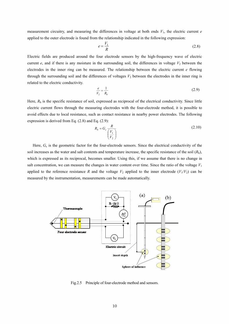
Here, Gc is the geometric factor for the four-electrode sensors. Since the electrical conductivity of the soil increases as the water and salt contents and temperature increase, the specific resistance of the soil (Rb), which is expressed as its reciprocal, becomes smaller. Using this, if we assume that there is no change in salt concentration, we can measure the changes in water content over time. Since the ratio of the voltage V1 applied to the reference resistance R and the voltage V2 applied to the inner electrode (V1/V2) can be measured by the instrumentation, measurements can be made automatically.
Fig.2.5 Principle of four-electrode method and sensors.
11
In the measurement display area on the portable soil electric conductivity meter shown in Fig. 2.5(a), a battery is used as the power source, and the ratio of voltages (V1/V2) is calculated by the elements built into the integrated circuitry. On site, an auger slightly more fine than the four-electrode sensors on the portable soil electrical conductivity meter, with 10mm of outer diameter, is used, into which sensor insertion holes are opened to the depth to be measured, the portable soil electrical conductivity meter is inserted, and the values are read from the display. On site, several measurement spots are selected on a plane, and the electrical conductivity is measured. If the value for any measured point is markedly different from any other point, core soil sampling is performed at the location, and the apparatus can be used as a preliminary tool for performing more detailed physical and chemical examinations of the soil.
With the multipoint four-electrode sensors shown in Fig. 2.5(b), a data logger and multiplexer can be used to automatically measure the electrical conductivity and temperature distribution in the soil at the same time. When the salt concentration can be ignored, there are cases where the dynamic fluctuations in vertical moisture distribution after rainfall have been recorded at multiple points with no time lag, making this method applicable for long-term fixed-point observation.
As described above, although the method for measuring electrical resistance in soil (the reciprocal of electrical conductivity) has an effect on the temperature and solution concentration in the material being measured, if there are no significant changes in the solution concentration, this apparatus can be used as a moisture content meter by performing a temperature conversion.
2.6 Capacitance method
Since the dielectric constant is approximately 81 for water, approximately 3 to 5 for dried soil, and approximately 1 for air, the capacitance method is a method for measuring moisture using the fact that the dielectric constant increases as water content increases. As shown in the following expression, capacitance (C) is proportional to the dielectric constant (Kd).
C = Gc Kd (2.11) Here, Gc is a shape factor that is dependent on the size and shape of the capacitance sensor and the distance between the electrodes. Many commercially available capacitance type moisture measuring systems resonating LC circuitry, and are manufactured so that the change in the capacitance of the soil relates to the changes in the resonating frequency of the circuitry. The maximum voltage production frequency f for the resonance is:
CLf
Cπ21
= (2.12)
Here, Lc is inductance [μH], and its units H (Henry) indicate the magnetic permeability of the coil. The dielectric constant is determined according to the water retention of the soil, capacitance C is determined from Eq. (2.11), frequency f is determined from Eq. (2.12), electronic circuitry is used to change the frequency to voltage, and by correlating the measured voltage and water content, the capacitance sensors can be used to measure the water content of the soil.
In particular, there are also measurement instruments in which the parallel plate has been designed on a cyclic conductor and the sensors inserted into the access tube so that measurements can be made on site (See Fig. 2.6(b)). Although there are differences due to probe design, the frequency is in the range of
12
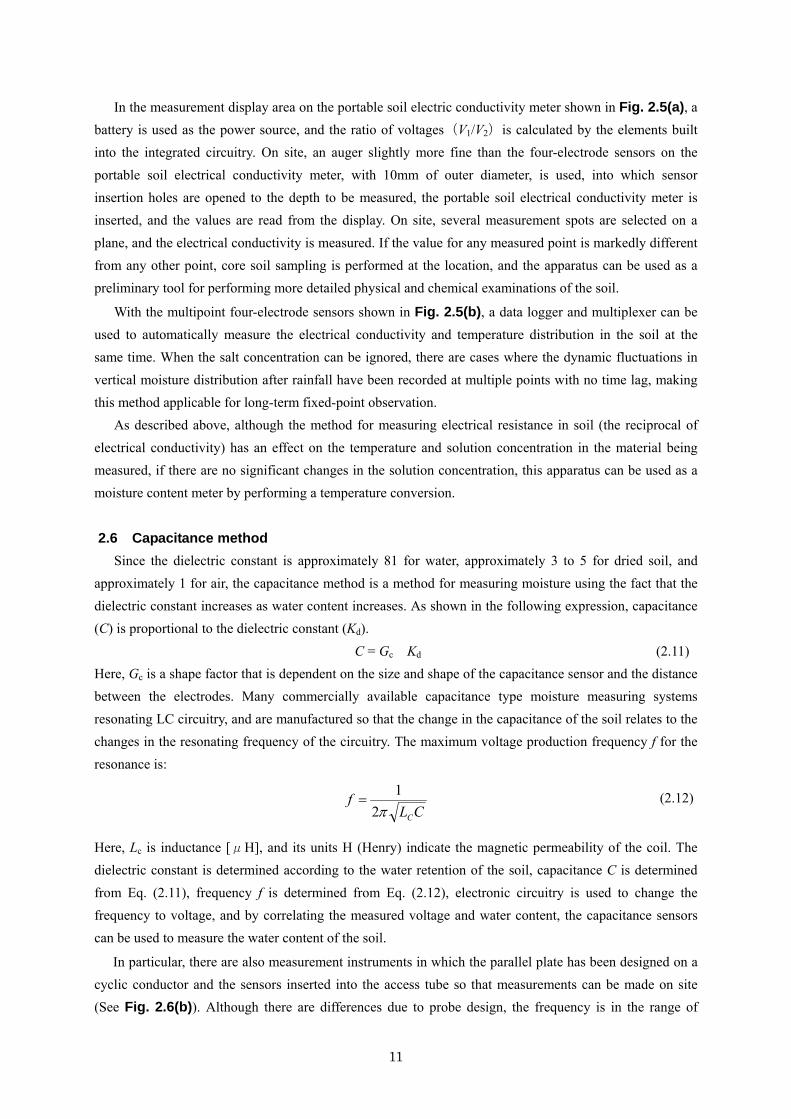
38MHz to 150MHz. Capacitance sensors are available in a variety of shapes, and can be grouped into parallel rod types, cylindrical ring types, and flat types, as shown in Fig. 2.6. The parallel rod types have 2, 3, or 4 metallic rod sensors. Since electronic circuitry is included in the sensors of each type, they are simple measuring systems in which the user needs only provide a battery for applied voltage and a data logger for measuring the output voltage.
Fig. 2.6 Soil moisture sensors based on capacitance method. In order to measure the water content of soil in deep layers on site, the cylindrical ring type capacitance
sensors are effective. If the capacitance sensor is inserted into a vinyl access tube, the frequency is measured for water only, air only, and soil, then the frequency is normalized with the following expressions, allowing the removal of individual differences of sensors and improvement of measuring precision.
wa
saS ff
ffF
−−
= (2.13)
bSFa=θ (2.14)
Here, FS is the normalized universal frequency, fa is the frequency reading in air, fs is the frequency reading in soil, fw is the frequency reading in water, and a and b are fitting parameters.
If the value of FS/FSmax from Eq. 2.13 is used as the 99% or greater range of measurement influence of the profile probe shown in Fig. 2.6(b), the radius is 10cm in the horizontal direction, and the height is 5cm in the vertical direction. There are also profile probes in which the depth is set at the following 5 points: 10cm, 20cm, 30cm, 40cm, and 50cm. The flat type capacitance sensor shown in Fig. 2.6(c) is an inexpensive and simple system for measuring moisture in soil. However, if fertilizer is added to the soil, the output value from the measuring device will drop for some sensors even if the water content is the same. Therefore, it is necessary to carefully consider which sensor to use based on the purpose of the measurements to be made. This effect due to fertilizer will be discussed in a later section.
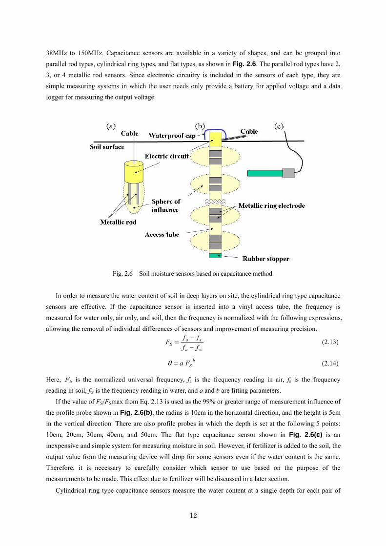
Cylindrical ring type capacitance sensors measure the water content at a single depth for each pair of
13
ring electrodes. As shown in Fig. 2.7, there are also measurement systems available where measurements can be performed to a maximum of 30m at a maximum 16 depths (depth can be set freely every 10cm) for a single point, and cables can be extended to a maximum 500m.
Fig.2.7 Soil moisture measurement system in a sloping cross-section using capacitance sensors. 2.7 Dielectric method
The dielectric constant is a specific value for each material, as follows: air 1, water 80 (20°C), ice 3 (-5°C), basalt 12, granite 8, and sandstone 10. Therefore, the dielectric method uses the fact that the dielectric constant increases as the water content in soil increases. There are three methods for making electrical measurements of the dielectric constant: the TDR (time domain reflectometry method) method, the FDR (frequency domain reflectometry method) method, and the ADR (amplitude domain reflectometry method) method.
2.7.1 Time domain reflectometry method
The TDR method measures the apparent dielectric constant by measuring within the time region the round trip rate of electromagnetic waves at a constant frequency (a high frequency from 30MHz to 3GHz) to and from rods (metal electrodes) buried in the soil.
The measurement system is made up of a cable tester that produces high-frequency electromagnetic pulses and monitors reflected waves, rods inserted into the soil, and coaxial cable connecting the cable tester and rods. The connections between the coaxial cable and rods must be fixed with epoxy to prevent short circuits, and be designed to produce clear peaks in the waveform. The rods area contains signal rods and shield rods. Systems are available with one, two, or three shield rods.
The dielectric constant (Kd) is found with the following expression:
protector
14
22
02
0
2 ⎟⎟⎠
⎞⎜⎜⎝
⎛=⎟
⎠
⎞⎜⎝
⎛=⎟
⎠
⎞⎜⎝
⎛=
p
ad LV
LL
tcv
cK
Δ (2.15)
where, c0 is the velocity of electromagnetic waves in free space [3 × 10⁸ m/s], v is propagation velocity [m/s], Δt is the round trip time of the electromagnetic pulse [ns], L is the length of the sensor rod [m], La is the apparent probe length [m], and Vp is the relative propagation velocity (Vp = 1.0 is used to measure water content), Δt in Eq. 2.15 is measured in units of ns (one billionth of a second), and therefore a highly-precise and expensive cable tester is required.
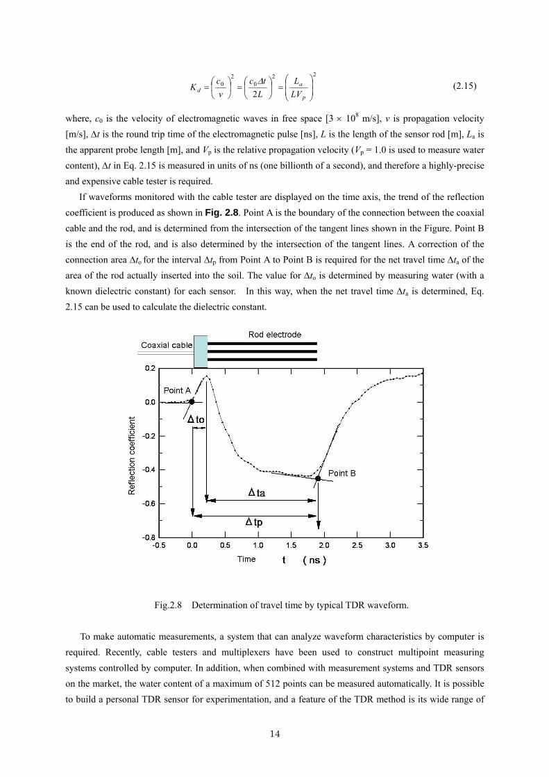
If waveforms monitored with the cable tester are displayed on the time axis, the trend of the reflection coefficient is produced as shown in Fig. 2.8. Point A is the boundary of the connection between the coaxial cable and the rod, and is determined from the intersection of the tangent lines shown in the Figure. Point B is the end of the rod, and is also determined by the intersection of the tangent lines. A correction of the connection area Δto for the interval Δtp from Point A to Point B is required for the net travel time Δta of the area of the rod actually inserted into the soil. The value for Δto is determined by measuring water (with a known dielectric constant) for each sensor. In this way, when the net travel time Δta is determined, Eq. 2.15 can be used to calculate the dielectric constant.
Fig.2.8 Determination of travel time by typical TDR waveform.
To make automatic measurements, a system that can analyze waveform characteristics by computer is required. Recently, cable testers and multiplexers have been used to construct multipoint measuring systems controlled by computer. In addition, when combined with measurement systems and TDR sensors on the market, the water content of a maximum of 512 points can be measured automatically. It is possible to build a personal TDR sensor for experimentation, and a feature of the TDR method is its wide range of
15
application to measurements in both laboratory testing and on-site testing. For example, one can build a small TDR sensor for laboratory experiments, to measure moisture behavior. There have also been cases where small coil type TDR sensors (15mm in length, 3.6mm in diameter) have been developed. With the use of such small TDR sensors, there is hope for experimentation to examine detailed moisture distribution, such as the fingering phenomenon in two-dimensional earth tanks.
The TDR method has the following features and advantages: (1) Use of a calibration curve specific to soil allows highly precise measurements with a measurement error of 0.01 to 0.02cm3/cm3 for volumetric water content, (2) rapid measurements are possible, allowing continuous measurement of the dynamic state of water after rainfall, and (3) measurement of the average water content in the soil along the length of the rod is possible. On the other hand, problems include: (1) The equipment is expensive, (2) not easily applicable to soil with a high salt concentration (for a rod length of 30cm the electrical conductivity is 4 dS/m or greater, preventing accurate measurement), (3) it is dependent on temperature, (4) additional calibrations are required for soil that has a lot of volcanic ash or organic content, (5) measurement is difficult when the soil at the ends of the rod becomes extremely dry, and (6) measurement is difficult when the ends in stratified soil are dried.
2.7.2 Frequency domain reflectometry method
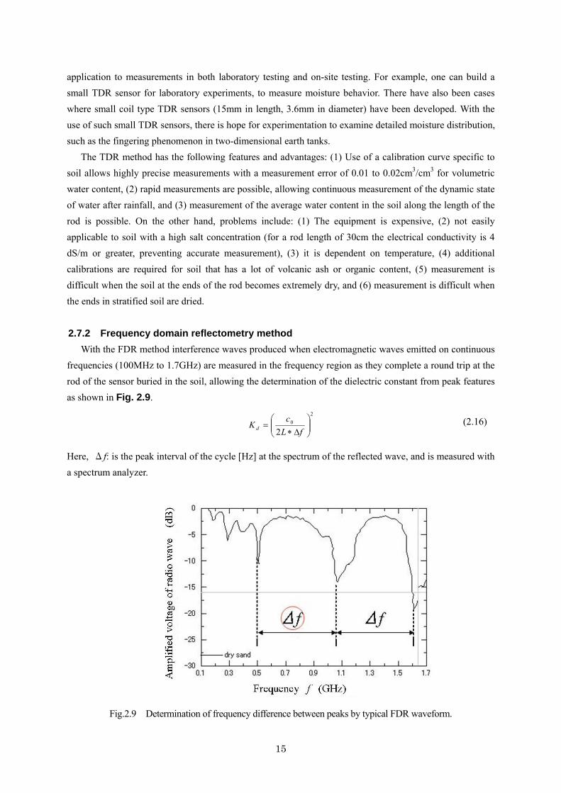
With the FDR method interference waves produced when electromagnetic waves emitted on continuous frequencies (100MHz to 1.7GHz) are measured in the frequency region as they complete a round trip at the rod of the sensor buried in the soil, allowing the determination of the dielectric constant from peak features as shown in Fig. 2.9.
20
2 ⎟⎟⎠
⎞⎜⎜⎝
⎛Δ∗
=fL
cK d
(2.16)
Here, Δf: is the peak interval of the cycle [Hz] at the spectrum of the reflected wave, and is measured with a spectrum analyzer.
Fig.2.9 Determination of frequency difference between peaks by typical FDR waveform.
16
2.7.3 Amplitude domain reflectometry method The ADR method is used to find the dielectric constant by measuring in the amplitude region the difference in voltage (vj−vo) produced when electromagnetic waves at a constant frequency (100MHz) make a round trip at the rod of the sensor buried in the soil.
⎟⎟⎠
⎞⎜⎜⎝
⎛+−
==−
⎟⎟⎠
⎞⎜⎜⎝
⎛⎟⎟⎠
⎞⎜⎜⎝
⎛=
LP
LPj
CP
d
IIII
aavv
rr
GlnI
K
22
60
0
2
1
2
ρ (2.17)
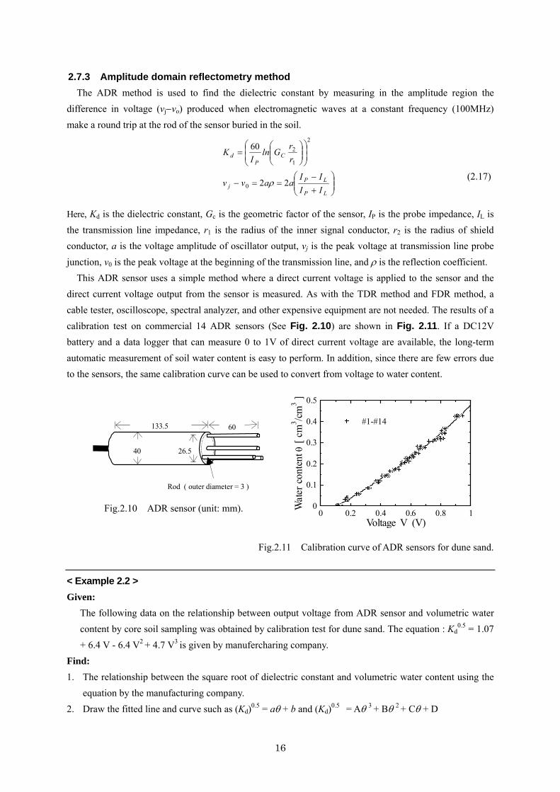
Here, Kd is the dielectric constant, Gc is the geometric factor of the sensor, IP is the probe impedance, IL is the transmission line impedance, r1 is the radius of the inner signal conductor, r2 is the radius of shield conductor, a is the voltage amplitude of oscillator output, vj is the peak voltage at transmission line probe junction, v0 is the peak voltage at the beginning of the transmission line, and ρ is the reflection coefficient. This ADR sensor uses a simple method where a direct current voltage is applied to the sensor and the direct current voltage output from the sensor is measured. As with the TDR method and FDR method, a cable tester, oscilloscope, spectral analyzer, and other expensive equipment are not needed. The results of a calibration test on commercial 14 ADR sensors (See Fig. 2.10) are shown in Fig. 2.11. If a DC12V battery and a data logger that can measure 0 to 1V of direct current voltage are available, the long-term automatic measurement of soil water content is easy to perform. In addition, since there are few errors due to the sensors, the same calibration curve can be used to convert from voltage to water content.
Fig.2.10 ADR sensor (unit: mm).
Fig.2.11 Calibration curve of ADR sensors for dune sand.
< Example 2.2 > Given:
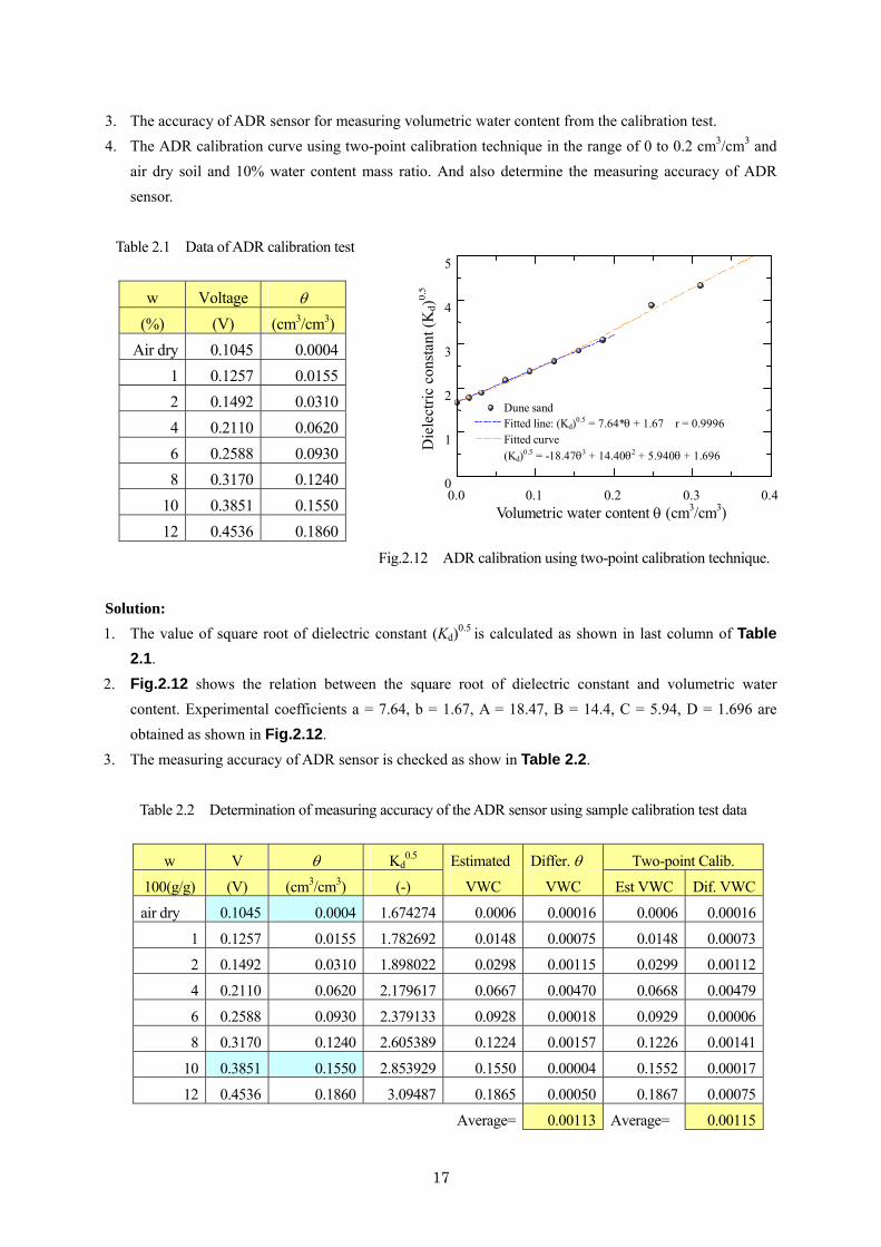
The following data on the relationship between output voltage from ADR sensor and volumetric water content by core soil sampling was obtained by calibration test for dune sand. The equation : Kd
0.5 = 1.07 + 6.4 V - 6.4 V2 + 4.7 V3 is given by manufercharing company.
Find: 1. The relationship between the square root of dielectric constant and volumetric water content using the
equation by the manufacturing company. 2. Draw the fitted line and curve such as (Kd)0.5 = aθ + b and (Kd)0.5 = Aθ 3 + Bθ 2 + Cθ + D
3. The accuracy of ADR sensor for measuring volumetric water content from the calibration test. 4. The ADR calibration curve using two-point calibration technique in the range of 0 to 0.2 cm3/cm3 and
air dry soil and 10% water content mass ratio. And also determine the measuring accuracy of ADR sensor.
Fig.2.12 ADR calibration using two-point calibration technique.
Solution: 1. The value of square root of dielectric constant (Kd)0.5 is calculated as shown in last column of Table
2.1. 2. Fig.2.12 shows the relation between the square root of dielectric constant and volumetric water
content. Experimental coefficients a = 7.64, b = 1.67, A = 18.47, B = 14.4, C = 5.94, D = 1.696 are obtained as shown in Fig.2.12.
3. The measuring accuracy of ADR sensor is checked as show in Table 2.2. Table 2.2 Determination of measuring accuracy of the ADR sensor using sample calibration test data
w V θ Kd0.5 Estimated Differ. θ Two-point Calib.
100(g/g) (V) (cm3/cm3) (-) VWC VWC Est VWC Dif. VWC
air dry 0.1045 0.0004 1.674274 0.0006 0.00016 0.0006 0.00016
The Estimated VWC value of fifth column is calculated from Eq.(2.18) based on the fitted line shown in Fig.2.12. The Difference VWC value of the sixth column is the absolute value of difference between measured volumetric water content θ and estimated volumetric water content, Dif. VWC.
647671744646071 32
..)V.V.V..( −+−+
=θ (2.18)
The difference between measured and estimated values using Eq.(2.18) is smaller than 0.005 cm3/cm3 and the average value of this difference is 0.00113 cm3/cm3.
4. An easier calibration method is the two-point calibration technique using equation: (Kd)0.5 = aθ + b. Using the data for air dry soil and 10% water content mass ratio, experimental coefficients a and b can be obtained from [(Kd)0.5]0 = 1.674, θ 0 = 0.0004, [(Kd)0.5]10 =2.854, θ 10 = 0.155. The results shows that a = 7.63 and b = 1.67.
The measuring accuracy of the ADR sensor using the two-point calibration technique is almost same as that of the calibration test.
2.7.4 Problems of dielectric method (1) Temperature dependency
The dielectric constant is dependent upon temperature T. The dielectric constant Kd of water in soil drops as temperature rises in the range from 0°C to 100°C, falling linearly within a certain range as shown in Fig. 2.13.
Fig.2.13 Relationship between dielectric constant of water and temperature.
The straight line in the figure indicates the temperature dependency in the following expression: Kd(T) = 87.740 - 0.40008 T + 9.398 × 10⁻⁴ T2 - 1.410 × 10⁻⁶ T3 (2.19)
In the range of 5°C to 50°C, 25°C is considered the standard for the dielectric constant of water, and conversion is possible with the following relational expression:
On the effects of temperature on the dielectric constant of soil, Wraith and Or (1999) separated water into
19
combined water and free water, and used a 4-phase mixed model to speculate on temperature dependency. Yamanaka (2003) used an experimental model through multiple regression analysis with water content of soil and saturated hydraulic conductivity as explanatory variables to attempt temperature conversion, but had difficulty with quantitative conversion. (2) Relationship between volumetric water content and dielectric constant
An experimental method is described below for the relationship between volumetric water content (θ) and the dielectric constant of soil (Kd). Topp et al. (1980) came up with the following empirical formula for multiple soil samples:
3 (2.21) Volumetric water content from Eq. (2.20) tends to produce underestimations for a soil that is rich in organic material such as kuroboku soil (volcanic ash soils) and viscous soil. Miyamoto et al. (2001) provided the following calibration formula for kuroboku soil:
3 (2.22) Yu et al. (1997) suggested the following empiric formula (a and b are fitting parameters.):
θ = a Kdγ + b (2.23)
(3) Dry bulk density dependency In addition to the dependency of the dielectric constant of soil on water content and temperature as
described above, it is also dependent on dry bulk density. Malicki et al. (1996) suggested the following empirical formula for a wide range of soils, from soil that contains organic material to sand, with a dry bulk density in the range of 0.13 to 2.67g/cm3:
d
ddd
.....K
ρρρ
θ181177
159016808190 2
+
−−−= (2.24)
Here, ρd is the bulk dry density of soil. As dry bulk density increases, volumetric water content also increases. For example, if the dielectric constant for soil is 15 and the dry bulk density increases by 0.1g/cm3, the volumetric water content also increases by about 0.01cm3/cm3. (4) Influence of solution concentration
If salt is contained in the soil solution, the dielectric constant changes and the calibration formula for estimating water content is affected. In addition, if the salt concentration is high, the coefficient of reflection shown to the right of Point B in Fig. 2.8 becomes smaller, and the presence of Point B becomes obscure and impossible to measure. For example, a waveform analysis using TDR100 is shown in Fig. 2.14 for the water solution with a salt concentration different from NaCl. Here, the rod length is 6cm, and the offset value is 7cm. If the salt concentration is 30,000ppm (near the concentration for seawater), it is understandable that Point B cannot be found.
The standard rod length is 10cm to 30cm, and the interval between rods is 10 times the rod diameter or less, within a range of 1.5cm to 10cm. If the rod length is too long, the transmission time for soil that includes electrolytes cannot be determined. Fig. 2.15 shows the maximum rod length is dependent on volumetric water content and electrical conductivity, as reported in Dalton and van Genuchten (1986). For example, for an electrical conductivity of 20 dS/m and a volumetric water content of 0.4cm3/cm3, the water content cannot be measured for a rod longer than 9cm. Methods for making a slight improvement include shortening the rod length, or using a heat-shrink tube to wrap the signal rod. In addition, it is important to
20
evaluate to what extent the dielectric constant measurement system being used is affected by salt, and the measuring precision of the instrumentation. As a result of examining the effect of salt on the measurement of water content in sand, Inoue (1998) reported that salt has little affect on dielectric constant measurements performed with the ADR method with a NaCl solution of 5000ppm up to an electrical conductivity of 9 dS/m. This is discussed in a later section.
Fig. 2.14 TDR waveform analysis at different NaCl (ppm).
(5) Influence of layered soil In general, TDR moisture sensors measure the average water content at the sensor. However, if the sensor
is inserted perpendicularly in stratified soil, measurement will not be possible if the soil at the end of the sensor is dry. Accurate measurement is not possible if there is wet soil on top of the dry soil. When measuring the water content of a stratified soil, more accurate moisture measurements can be made by setting the sensor horizontally and performing calibrations for each soil sample. (6) Influence of clearance between sensor and soil
If the rod area of the sensor is inserted into the soil, any small clearance between the rod and soil will affect the measurement. For example, it has been reported that if there is a clearance of 0.5mm between the sensor and the soil, the dielectric constant will drop to 1/4. It has also been reported that the flat type dielectric constant sensor shown in Fig. 2.6(c) cannot make measurements if the soil becomes dry and a clearance develops between sensor and soil, in particular when measuring the moisture in a viscous soil. Therefore, it is important to consider the target soil characteristics and moisture range when selecting a sensor shape.
2.7.5 Characteristics and measurement system of a dielectric moisture probe Dielectric moisture probes are frequently used as moisture meters in laboratory and on-site testing due to
the fact that there is no danger from radiation such as with the neutron method or gamma rays, and the recent development of a variety of probes. The TDR method is used to find the dielectric constant by measuring in the time region the speed of electromagnetic waves at a constant frequency as they make a round trip to the measuring electrodes of the sensors buried in the soil. Expensive cable testers are required for this method, as well as special software for processing waveforms. Further, the empirical formula
Fig.2.15 Maximum rod length depend on volumetric soil water content and electrical conductivity.
suggested by Topp et al. (1980) is often used for the relationship between dielectric constant and volumetric water content. However, a calibration curve different from the Topp et al. (1980) formula has recently been found for volcanic ash and soil rich in organic matter. A method for measuring dielectric constant has been developed without the use of expensive oscilloscopes and cable testers. The ADR method is used to find the dielectric constant by measuring in the amplitude region the difference in voltage produced when electromagnetic waves at a constant frequency (100MHz) make a round trip at the measurement electrode of the sensor buried in the soil.
Fig. 2.16 Different type of dielectric probes and measuring system Recently, there has been rapid expansion in measurement technology for dielectric constant. Typical
sensor shapes and measurement systems are shown in Fig. 2.16. In Fig. 2.16(a), a special table tester including a pulse generator, reflected wave receiver, and monitor is required, and is connected to the sensor by a coaxial cable. In order to measure water content, waveforms are processed using special software, and the user can select the shape of the probe. Noborio (2003) describes the probe design. Sensors have been developed with different shape, and are available with two, three, or four metal rods. There are several types of sensors for research, such as sensors installed on Cone penetrometers (Carlos et al., 2001), sensors wound on porous cup of tensiometers (Carlos et al., 2002), and sensors combined with heaters and thermocouples in rods (Ren et al., 1999). These sensors were developed to perform simultaneous measurement of water content, salt content, potential, soil bearing capacity, soil temperature, and heat conduction coefficient on site.
Fig. 2.16(b) shows a system with a rectangular stick-type probe 150cm in length and measurement display, for the simultaneous measurement of volumetric water content in ranges of 0 to 15cm, 15 to 30cm, 30 to 60cm, 60 to 90cm, and 90 to 110cm. Several of the rectangular stick-type probes can be buried in the soil on site, and the measurement display added/removed while performing manual measurements, or the measurement display can be connected to a data logger for fixed-point observation while collecting the data on computer via an RS232C cable.
Fig. 2.16(c) shows a measurement system that is applicable for the automatic recording of water
22
content at multiple points on site simultaneously. The shape of the sensor is three metal rods (3.2mm outer diameter, 300mm length, and 60mm width, for example), and up to 64 points can be measured for water and salt content with the use of the measuring apparatus, a data logger, and 9 multiplexers. The range of measuring influence for the sensor is roughly restricted by the length of the rod, and the average water content in the direction of the rod is measured. Therefore, if the sensor is buried vertically, the average water content of the entire 30cm soil layer is measured, and if the sensor is buried horizontally, the average water content is measured at a thickness of 2cm for that depth. The user can design a unique sensor by setting the offset value and sensor constant.
Fig. 2.16(d) shows a measuring system applicable for burying several access tubes in advance on site, inserting measurement sensors, and using a measurement display to manually measure the moisture profile. There are two types of moisture profile meters commercially available: one that can measure at depths of 10cm, 20cm, 30cm, 40cm, 60cm, and 100cm, and one that can measure at depths of 10cm, 20cm, 30cm, and 40cm. The range of measurement influence is a 5cm radius vertically, and a 7cm radius horizontally. They are connected to an applied voltage device (DC 5 V to 9 V) and a data logger; fixed-point observation is performed, and the data is collected by computer via a special cable.
Fig. 2.16(e) shows a measuring system that can perform portable moisture measurements (including sensors that can measure salt). For sensors that can be used for special purposes, there are sensors that can simultaneously measure moisture, salt, EC, and temperature, as well as multiple function sensors that can simultaneously measure dielectric constant, apparent electrical conductivity, electrical conductivity of soil solutions, volumetric water content, and soil temperature.
The type of sensor and measuring system that should be used depend on the measurement precision required by the user, as well as budget and purpose. As mentioned earlier, water content measurements using dielectric constant are affected by salt content, temperature, dry bulk density, and clearance between the sensor and the soil. However, if the user determines that a measurement error of ±0.03 cm3/cm3, for example, is sufficient for volumetric water content, there are many sensors that can be utilized in that range. Selection can also be made on the purpose of the measurement. For example, to measure water content to a depth of 20m, a cylindrical ring type capacitance sensor would be selected.
For water content measurement sensors and measuring systems, it is vital for the user to make a determination after collecting information such as the range of measurement influence of the sensor (what area is being measured?), measurement precision (to what degree of reliability is measurement possible?), effects due to salt, organic matter, etc., and know-how for performing auto recording.
This concludes the description of dielectric constant moisture meters. Recently, these sensors have been used for the measurement of salt concentration, added to temperature sensors to simultaneously measure the temperature and coefficient of thermal conductivity in soil (Ren et al., 1999), and the measurement of the coefficient of dispersion contributing to the permeability and solute migration in soil.
2.8 Heat probe type soil moisture meter
Heat in soil flows from areas of high temperature to areas of low temperature. Thermal volume and heat flux [W/m], which intersect the cross section in units of time, are proportional to the temperature gradient [K/m], and that proportionality coefficient is called thermal conductivity [W/m/K]. Since the thermal conductivity of the gas phase is much smaller than the thermal conductivity of the liquid and solid phases,
23
thermal conductivity increases as water content in the soil increases. The relationship between water content and thermal conductivity differs according to both the type of soil and temperature. However, while changes in soil temperature are small in the same type of soil, the change in thermal conductivity due to changes in water content are large, and therefore this relationship can be used as a gauge of water content.
In order to actually measure water content, it is necessary to know the relationship between water content and thermal conductivity in advance, and measure the thermal conductivity of the target being measured. There are three methods for measuring thermal conductivity: the heat probe method, dual heat probe method, and simple thermal conductivity measurement method. By inserting a probe equipped with a heater and thermometer into the soil and supplying an electric current to the heater to raise the temperature, if there is a lot of surrounding moisture the thermal conductivity of the soil will be large, the heat from the probe will be transmitted to the surrounding area, and the rising temperature of the probe will be contained. Thermal conductivity can be measured by measuring the change in temperature in the sensor when applying heat in pulses. With the dual heat probe method, the thermal conductivity of the standard material is measured regardless of the target material being measured, the irreversible error of the probe is offset, and the measuring precision is improved.
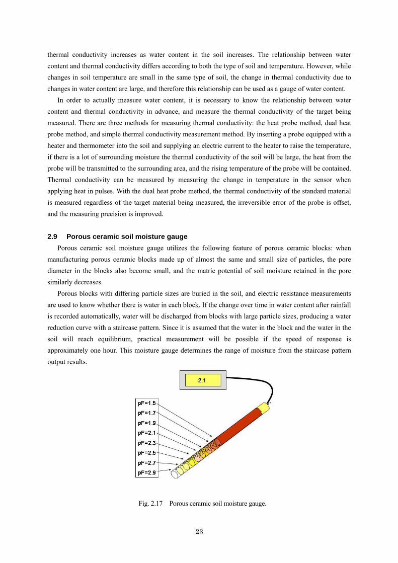
2.9 Porous ceramic soil moisture gauge
Porous ceramic soil moisture gauge utilizes the following feature of porous ceramic blocks: when manufacturing porous ceramic blocks made up of almost the same and small size of particles, the pore diameter in the blocks also become small, and the matric potential of soil moisture retained in the pore similarly decreases.
Porous blocks with differing particle sizes are buried in the soil, and electric resistance measurements are used to know whether there is water in each block. If the change over time in water content after rainfall is recorded automatically, water will be discharged from blocks with large particle sizes, producing a water reduction curve with a staircase pattern. Since it is assumed that the water in the block and the water in the soil will reach equilibrium, practical measurement will be possible if the speed of response is approximately one hour. This moisture gauge determines the range of moisture from the staircase pattern output results.
Fig. 2.17 Porous ceramic soil moisture gauge.
24
As shown in Fig. 2.17, moisture gauges that are available use ceramic blocks with eight types of different particle sizes. The range from pF1.5 to pF2.9 corresponds with an output voltage from 0 (V) to 1 (V), and the water content of soil is output in pF units of 0.1. Basically, it is assumed that the water in the ceramic block and water in the soil will reach equilibrium, and there are effects due to time lag and temperature. However, this differs according to the type of soil, and practical measurement is possible if there is approximately 3 hours available for measurement.
Since porous ceramic soil moisture gauges measure the electric resistance in ceramics buried in soil, a remarkable change in temperature will have a large impact. Further, if the soil has a high salt concentration, additional calibrations will be necessary.
< Example 2.3 > Given:
Waveform using TDR100 (Campbell Co. Ltd.) and TDR sensor (Sankeirika Co. Ltd.) as shown in Fig.2.18.
Fig. 2.18 Waveform analysis for volumetric soil water content of 0.21 Find:
1. The dielectric constant Kd using Eq. (2.15), where, Vp = 1.0 and the rod length is 0.06m. 2. Volumetric soil water content θ, when the relationship between θ and Kd was previously given
by the calibration experiment as follows: θ = − 0.000824 Kd 2 + 0.0431 Kd − 0.125.
Solution: 1. La = 0.184, L = 0.06, Vp = 1.0 as shown in Fig. 2.18. Dielectric constant Kd = (La /L /Vp)2 =
(0.184/0.06/1.0)2 = 9.4 2. Volumetric soil water content
where, z is soil depth, distance from soil surface to the center of sampler (cm), Wa is total mass of soil sample plus the cylinder with saucer (g), Wb is total mass of dry soil sample plus the cylinder with saucer (g), Wc is mass of the cylinder with saucer (g). Find: 1. The water content mass ratio w, volumetric water content θ, and soil water storage Wz on 6 June, 1990.
z Ms Mw W ρb θ Wz
(cm) (g) (g) (g/g) (g/cm3) (cm3/cm3) (mm)
5
15
25
35
50
Where, Ms is total mass of dry soil sample (g), Mw is mass of soil water in the soil sample (g), w is water content mass ratio (g/g), ρb is dry bulk density (g/cm3), and Wz is soil water storage (mm).
2. The water content mass ratio w, volumetric water content θ, and soil water storage Wz on 6 Oct., 1990.
z Ms Mw W ρb Θ Wz
(cm) (g) (g) (g/g) (g/cm3) (cm3/cm3) (mm)
5
15
25
35
50
< Example 2.4 > Given: Volumetric water content at several depths, θz as shown in Table 2.3. Find: 1. The soil water storage Wz for each layer
2. The soil water storage W from z = 0 to zr = 60 cm Solution: As soil samplings are taken at the depth of 5, 15, 25, 35, 50 cm, soil water storage W is calculated as follows
26
0
rzW dzθ= ∫ (2.25)
Table 2.3 Calculation of soil water storage
depth z (cm)
Layer (cm)
thickness dz (mm)
θz
(cm3 /cm3) soil water storage Wz
(mm)
5 15 25 35 50
0-10 10-20 20-30 30-40 40-60
100 100 100 100 200
0.059 0.085 0.124 0.157 0.163
5.9 8.5
12.4 15.7 32.0
Soil water storage W = 75.1
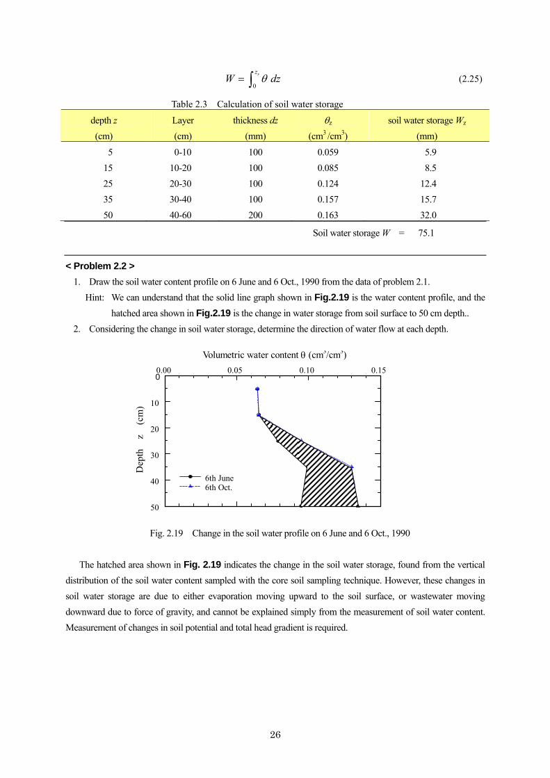
< Problem 2.2 > 1. Draw the soil water content profile on 6 June and 6 Oct., 1990 from the data of problem 2.1.
Hint: We can understand that the solid line graph shown in Fig.2.19 is the water content profile, and the hatched area shown in Fig.2.19 is the change in water storage from soil surface to 50 cm depth..
2. Considering the change in soil water storage, determine the direction of water flow at each depth.
Fig. 2.19 Change in the soil water profile on 6 June and 6 Oct., 1990
The hatched area shown in Fig. 2.19 indicates the change in the soil water storage, found from the vertical distribution of the soil water content sampled with the core soil sampling technique. However, these changes in soil water storage are due to either evaporation moving upward to the soil surface, or wastewater moving downward due to force of gravity, and cannot be explained simply from the measurement of soil water content. Measurement of changes in soil potential and total head gradient is required.
0.00 0.05 0.10 0.150
10
20
30
40
50
Volumetric water content θ (cm3/cm3)
Dep
th
z (
cm)
6th June 6th Oct.
27
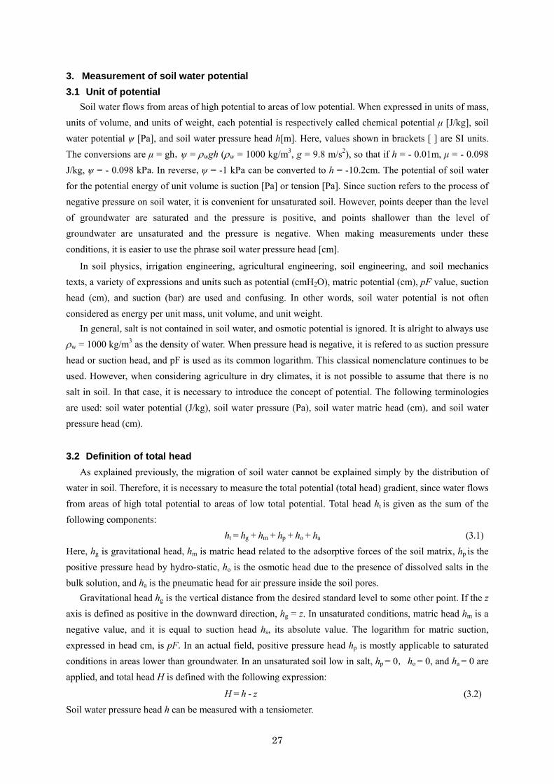
3. Measurement of soil water potential 3.1 Unit of potential
Soil water flows from areas of high potential to areas of low potential. When expressed in units of mass, units of volume, and units of weight, each potential is respectively called chemical potential μ [J/kg], soil water potential ψ [Pa], and soil water pressure head h[m]. Here, values shown in brackets [ ] are SI units. The conversions are μ = gh,ψ = ρwgh (ρw = 1000 kg/m3, g = 9.8 m/s2), so that if h = - 0.01m, μ = - 0.098 J/kg, ψ = - 0.098 kPa. In reverse, ψ = -1 kPa can be converted to h = -10.2cm. The potential of soil water for the potential energy of unit volume is suction [Pa] or tension [Pa]. Since suction refers to the process of negative pressure on soil water, it is convenient for unsaturated soil. However, points deeper than the level of groundwater are saturated and the pressure is positive, and points shallower than the level of groundwater are unsaturated and the pressure is negative. When making measurements under these conditions, it is easier to use the phrase soil water pressure head [cm].
In soil physics, irrigation engineering, agricultural engineering, soil engineering, and soil mechanics texts, a variety of expressions and units such as potential (cmH2O), matric potential (cm), pF value, suction head (cm), and suction (bar) are used and confusing. In other words, soil water potential is not often considered as energy per unit mass, unit volume, and unit weight.
In general, salt is not contained in soil water, and osmotic potential is ignored. It is alright to always use ρw = 1000 kg/m3 as the density of water. When pressure head is negative, it is refered to as suction pressure head or suction head, and pF is used as its common logarithm. This classical nomenclature continues to be used. However, when considering agriculture in dry climates, it is not possible to assume that there is no salt in soil. In that case, it is necessary to introduce the concept of potential. The following terminologies are used: soil water potential (J/kg), soil water pressure (Pa), soil water matric head (cm),and soil water pressure head (cm).
3.2 Definition of total head As explained previously, the migration of soil water cannot be explained simply by the distribution of
water in soil. Therefore, it is necessary to measure the total potential (total head) gradient, since water flows from areas of high total potential to areas of low total potential. Total head ht is given as the sum of the following components:
ht = hg + hm + hp + ho + ha (3.1) Here, hg is gravitational head, hm is matric head related to the adsorptive forces of the soil matrix, hp is the positive pressure head by hydro-static, ho is the osmotic head due to the presence of dissolved salts in the bulk solution, and ha is the pneumatic head for air pressure inside the soil pores.
Gravitational head hg is the vertical distance from the desired standard level to some other point. If the z axis is defined as positive in the downward direction, hg = z. In unsaturated conditions, matric head hm is a negative value, and it is equal to suction head hs, its absolute value. The logarithm for matric suction, expressed in head cm, is pF. In an actual field, positive pressure head hp is mostly applicable to saturated conditions in areas lower than groundwater. In an unsaturated soil low in salt, hp = 0,ho = 0, and ha = 0 are applied, and total head H is defined with the following expression:
H = h - z (3.2) Soil water pressure head h can be measured with a tensiometer.
28
3.3 Measurement of soil water pressure head 3.3.1 Tensiometer
A tensiometer is made up of a porous cup and a part for measuring the pressure inside the porous cup (See Fig.3.1). Livingston (1908) designed the current apparatus, and it is said that Gardner’s (1922) description of its functions resulted in the first tensiometer. Now, nearly a century have passed since then, but no practical instrument has been developed that can replace the tensiometer for the measurement of pressure head in soil. Here, pressure head is the pressure that indicates when the water is at equilibrium with soil water, and is a negative pressure in relation to atmospheric pressure. In general, the SI units for pressure are Pa (= N/m2). The relational expression 1kPa = 10.2 cmH2O is often used to convert this to a
head display (cmH2O), or in other words to convert it to pressure head. With a tensiometer, since the ceramic porous cup is generally buried in the soil and connected to a pressure gauge by a tube (PVC pipe is commonly used), the deaerated porous cup is filled with water in advance. If the tensiometer is inserted into unsaturated soil, the water pressure in the porous cup will be higher than the pressure of the soil water, and therefore the water will pass from the tensiometer, through the saturated porous cup, until equilibrium condition is achieved with the soil water. After rainfall or a moisturizing process such as irrigation, the direction of flow will reverse. In general, the water in the tensiometer is under negative pressure in unsaturated areas. This pressure (the difference with atmospheric pressure) is measured with a pressure gauge, such as a U-tube filled with water or mercury, a vacuum gauge (bourdon gauge), or a pressure (differential pressure) converter. (1) Tensiometer with mercury manometer
When using a U-tube filled with water or mercury, there is a large measurement time lag, and its degree is dependent on the permeability of the ceramic porous cup. Due to recent environmental issues, mercury manometers are no longer commonly used, but the measurement principles are easy to understand.
Calculating soil water pressure head h = -12.55 a + (b + z ) (3.3)
where a : reading of mercury manometer, b : distance of mercury surface to soil surface, z : depth of tensiometer cup
Fig.3.1 Tensiometer set with mercury manometer.
29
< Example 3.1 > Given:
Two tensiometers installed at the depth of 80 and 100 cm. a1 = 15cm, a2 = 16.5cm, b = 85 cm, z1 = 80 cm and z2 = 100 cm
Find: 1) Soil water pressure head h 2) Hydraulic head H 3) Hydraulic gradient dH/dz 4) Direction of flux
Solution: h, H and dH/dz are calculated using Eq.(3.3) as follows
The direction of flux is a downward flow, since the value of dH/dz is negative. If the value of dH/dz is positive, the direction of flux is an upward flow.
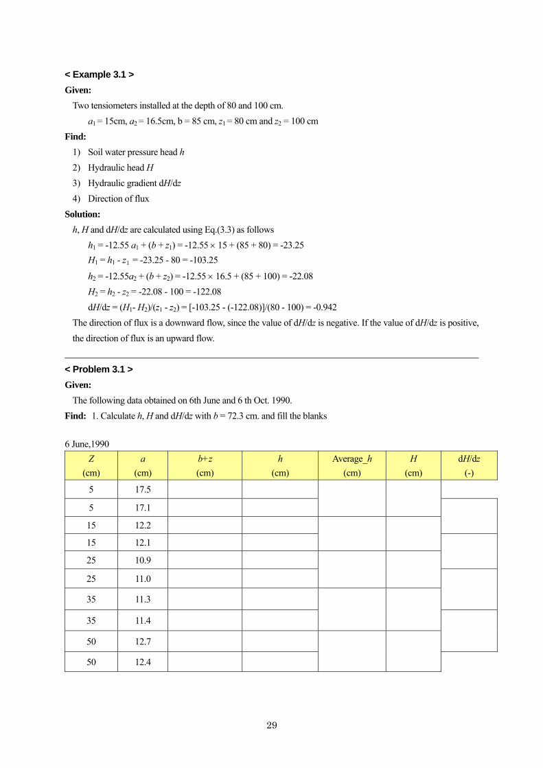
< Problem 3.1 > Given:
The following data obtained on 6th June and 6 th Oct. 1990. Find: 1. Calculate h, H and dH/dz with b = 72.3 cm. and fill the blanks 6 June,1990
Z a b+z h Average_h H dH/dz (cm) (cm) (cm) (cm) (cm) (cm) (-)
5 17.5
5 17.1
15 12.2
15 12.1
25 10.9
25 11.0
35 11.3
35 11.4
50 12.7
50 12.4
30
6 Oct,1990
Z a b+z h Average_h H dH/dz (cm) (cm) (cm) (cm) (cm) (cm) (-)
5 16.0
5 16.3
15 11.8
15 11.7
25 10.5
25 10.6
35 10.9
35 11.0
50 12.2
50 12.0
Find: 2. Draw the profile of hydraulic head and volumetric water content from 5 cm to 50 cm depth.
Hydraulic head H (cm) Volumetric water content θ (cm3/cm3)
-200 -150 -100 -50 0 0.05 0.1 0.15 0.2
Depth cm
10
20
30
40
50
31
If the soil becomes dry, the hydraulic flow between the water in the porous cup and the soil water will be lost, and measurement will not be possible. The range of measurement for a tensiometer depends on the characteristics of the ceramic porous cup. For example, depending on the air penetration value, 0.5bar, 1.0bar, and other tensiometers are available. With the former, measurements within a pressure head range of up to approximately -500cmH2O are possible, with good permeability and little time lag. For laboratory experiments, small-size tensiometers with pressure converters are commercially available. High-flow type porous cups are suitable for laboratory experiments, since the permeability and air penetration value of the porous cup are uniform and there is little individual difference. If a porous cup with insufficient dearation or poor permeability is used, air will penetrate during the experiment, and a time lag will occur in the measurement value. When measuring the changes in pressure head over time to determine the physical properties of soil using inverse analysis, it is important to rapidly change the water pressure and examine the response characteristics of each porous cup before performing an experiment. (2) Tensiometer with negative pressure gauge
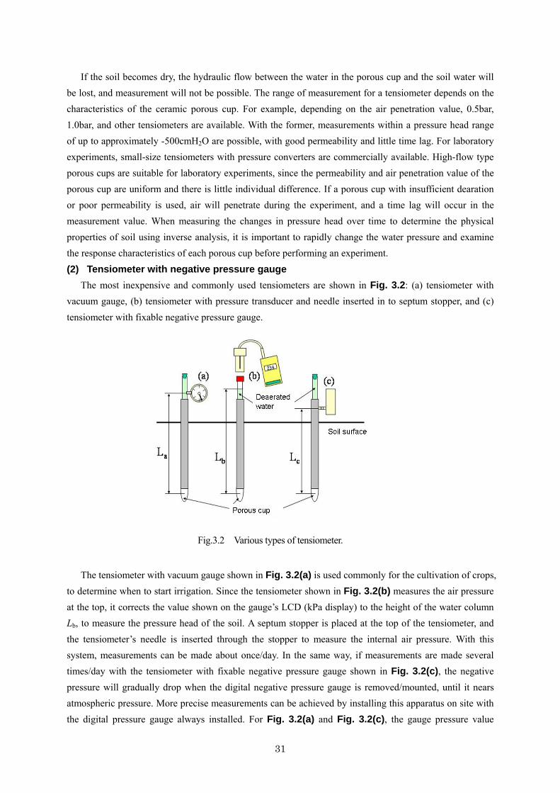
The most inexpensive and commonly used tensiometers are shown in Fig. 3.2: (a) tensiometer with vacuum gauge, (b) tensiometer with pressure transducer and needle inserted in to septum stopper, and (c) tensiometer with fixable negative pressure gauge.
The tensiometer with vacuum gauge shown in Fig. 3.2(a) is used commonly for the cultivation of crops, to determine when to start irrigation. Since the tensiometer shown in Fig. 3.2(b) measures the air pressure at the top, it corrects the value shown on the gauge’s LCD (kPa display) to the height of the water column Lb, to measure the pressure head of the soil. A septum stopper is placed at the top of the tensiometer, and the tensiometer’s needle is inserted through the stopper to measure the internal air pressure. With this system, measurements can be made about once/day. In the same way, if measurements are made several times/day with the tensiometer with fixable negative pressure gauge shown in Fig. 3.2(c), the negative pressure will gradually drop when the digital negative pressure gauge is removed/mounted, until it nears atmospheric pressure. More precise measurements can be achieved by installing this apparatus on site with the digital pressure gauge always installed. For Fig. 3.2(a) and Fig. 3.2(c), the gauge pressure value
Fig.3.2 Various types of tensiometer.
32
(converted to head) and the vertical distance La, Lc from the gauge’s installation position to the center of the porous cup are measured, and converted to pressure head. For Fig. 3.2(b), the position of the water surface is measured, corrected with the vertical distance Lb from the water surface to the center of the porous cup, and converted to pressure head. In each case, if the tensiometer is installed perpendicularly, it is necessary to correct the measurement value p (relative pressure of converted head) for the digital negative pressure gauge with the value for L in order to determine the value h of the pressure head.
h = p + L (3.4) For example, if the value of L shown in Fig. 3.2 is 100cm and the value (head conversion) read on the digital negative pressure gauge is -234cmH2O, the value for pressure head would be -134cmH2O, or pF = log (-h) = 2.13 when converted to pF value. If the measurement point becomes deep, the value for L gets larger, and even if pressure head is measured near saturated soil, the negative pressure level near the top of the tensiometer becomes larger. For example, when L = 1000cm, even if the value for pressure head is -10cm, the measured value (water head conversion) for the digital negative pressure gauge becomes -1010cm from Eq. (3.4), resulting in the measurement of condition that is close to a vacuum. Therefore, we can see that the limit for this measurement system is a depth of about 10m.
When soil is dried and the absolute value for pressure head becomes large, or when measuring a deep location, the negative pressure at the top of the tensiometer will increase, and therefore air is produced inside the tensiometer. It is necessary for the top of the tensiometer to have a transparent tube that allows the internal air to be seen, and a septum stopper or cock that allows the additional supply of degassed water is required.
When supplying degassed water, the pressure in the tensiometer would be released. To prevent this, the top is designed as a double tube with two cocks, and the bottom cock is used to supply water. When the system is sealed the upper cock is opened to refill the tube with degassed water.
Since tensiometers use water, there is the danger of freezing. To prevent this, Nakashima et al. (1995) reported that the use of propylene glycol solution is effective within a certain measurement range in an experiment under cold conditions. (3) Tensiometer with pressure transducer
There is a tensiometer with a digital negative pressure gauge that is always installed, with the same design as the removable digital negative pressure gauge shown in Fig. 3.2(c). This model includes a digital negative pressure gauge, which makes it expensive, but measurement precision is improved since the changes in pressure caused by the removal/attachment of the digital negative pressure gauge are prevented.
Automated recording is required when measuring pressure head in situ for long periods of time or through both day and night. The tensiometer shown in Fig. 3.2(c) is a commonly used model. For automatic recording, a measurement system that records an output voltage or output current from a pressure converter to a data logger is required. In general, a specific direct current voltage is applied to the voltage sensor, voltage is output according to the measured voltage, and this voltage is amplified and recorded as necessary. There are voltage sensors for -100kPa, -50kPa, and other measurement ranges, as well as those for positive pressure, negative pressure, and both positive and negative pressure. It is necessary to correct the relationship between pressure head (h) and output voltage (v) in advance.
The following linear expression is used for calibration in many cases: h = a V + b (3.5)
33
The correlation coefficient is high at 0.9999. Here, a and b are fitting parameters. When using this equipment, although there are some sensors that can be used simply by using the zero adjustment and trimmer adjustment, it is necessary to calibrate each sensor individually, and then perform a correction again for the value for the constant b in the expression for the known pressure head of the constructed system in actual measurement conditions, to develop a high-precision measurement system.
Fig. 3.3 Fluctuation of soil water pressure head reading due to hourly temperature variation.
As a measurement example, a porous cup was buried to a depth of 20cm, a data logger was connected to a fixable digital negative pressure gauge, and the pressure head was measured for 3 days, both day and night in clear weather. The trends in air temperature and results are shown in Fig. 3.3. This shows that the pressure head fluctuates 30cm or more with a change of 10°C between day and night. Tiny air bubbles formed at the top of the tensiometer, and it was affected by the differences in temperature between day and night. To prevent this, it was necessary to record the value of the tensiometer once every day at either 9am or 10am, for example, and reduce the effects due to temperature such as by shielding the top of the tensiometer from light and heat, and measuring the pressure head of the soil water, as shown by the arrows in the figure for example.
Fig.3.4 Buried-type tensiometer with pressure transducer.
34
The 38mm external diameter buried type tensiometer with pressure transducer (buried-type underground section gauge) shown in Fig. 3.4(b) was developed as a method for reducing the effects of temperature. Since this sensor includes temperature compensation circuitry, pressure head can be measured in a range up to -850cm at a precision of ±2cm for a change of 15°C. In addition, the pressure transducer is built into the porous cup, a design that makes it difficult to be affected by air temperature. The change in pressure head over time measured by the buried-type underground section gauge is shown in Fig. 3.3. It can be seen that effects due to temperature are reduced by a fluctuation of about 5cm in pressure head for a 10°C change in air temperature. This buried-type underground section gauge is applied to control water content in soil, in order to improve the yield and quality of vegetables (Nishihara et al., 2001). Since irrigation is frequently used in the cultivation of vegetables and drying is only allowed to about pF2, these sensors can be used all year without air penetrating the porous cup. However, if a significant amount of drying occurs, such as with the moisture control of trees, a negative pressure of -850cmH2O or less will occur, air will penetrate the porous cup, and measurement will not be possible. If this happens, a sensor that can refill degassed water into the porous cup is required. This type of tensiometer is also available. There are also dual buried type tensiometers with pressure transducers available that can refill the tube with degassed water, to accurately measure the dynamic water gradient between two points in the ground.
And, there are waterproof micro tensiometers (with porous cups of 6.3mm external radius and 10mm length) shown in Fig. 3.4(c), for use in small areas on site to measure pressure head in the soil. To remove even slight noise for precise measurements, a measurement system that can supply a stable voltage is required, and it is important to take measures against noise, such as providing an earth for the data logger. Recently, pressure sensors with temperature conversion circuitry have been used to precisely measure the pressure head in soil water with a resolution of 0.1cm and an error of 0.5cm, but such systems are not cheap. For self-recording tensiometers with pressure transducer shown in Fig. 3.2(c), it would be difficult to make measurements if the value for L in the figure approaches 10m, as mentioned before. However, for the buried type tensiometer with pressure transducer shown in Fig. 3.4, there is no restriction for burying depth, as long as the cord length is sufficient.
Pressure measurement systems for deep layer soil are also being tested overseas. A waterproof tensiometer with an external diameter of 25mm that can measure pressure within a range of 10kPa to -85kPa (Hobbell 1996) has been developed (See Fig. 3.4(a)). In addition, the micro tensiometer shown in Fig. 3.4(d) is also available. This is a model for burying in the soil, and makes it easy to automatically record the pressure head of soil water (Young 2002).
< Problem 3.2 > Given:
The following data obtained by calibration test using buried-type underground suction gauges (UNSUC). Find:
1) Calibration curves such as Eq.(3.5) for 8 sensors. 2) The measurement accuracy of UNSUC.
Fig.3.5 Calibration test of UNSUC (buried-type Underground Suction gauge).
(4) Buried-type underground suction gauge As shown in the right diagram of Fig. 3.6, buried-type underground suction gauges (UNSUC) have
expensive pressure receivers and electrical circuitry for converting pressure to voltage (pressure transducers) in their sensors, and a porous cylinder that can withstand a negative pressure of 1 bar. Special cords include a tube for atmospheric pressure, two wires (+ and -) for applied voltage (DC10V), and two wires (+ and -) for measuring output voltage. It is a simple measurement that applies a direct-current voltage (10V) to the sensors and reads the output voltage (from 0mV to 50mV). Measurements can be
36
made easily, with just a battery and a tester. Buried-type underground suction gauges consume 3mA/second each. In a farm, although it is preferred to observe with a battery, since 7000mA/s/(6 × 3mA/s) = 388.9 > 384h = 16day with a 7Ah battery, it can be seen that a battery cannot be used continuously for 10 days (16 days × 60% efficiency). Therefore, it is necessary to continually recharge the battery while using it, to include a preheat function so that the battery is consumed only while performing measurements, or to use a separate power supply such as a solar battery.
As shown in Fig. 3.5, a calibration box, water level adjustment tank, and a scale for measuring the level are provided to make calibrations. (1) Turn the sensor upside down, place it in the calibration box, use a screwdriver to remove the screws, and fill the calibration box with degassed water. (2) Use the bolts to fix the cover on the calibration box, seal the calibration box, and degas for 12 hours with a vacuum pump with a negative pressure of approximately 900cm. When air no longer comes out of the screw holes, the porous cylinder is saturated. At that time, if air penetrates through the O-ring on the calibration box, check for damage to the sensor and packing. (3) As shown in Fig. 3.5, use the pisco tube to connect the calibration box and water level adjustment tank. This completes the preparation for calibration. (4) When the water level in the water level adjustment tank is even with the center of the sensor (center of the porous cylinder), the pressure head is zero. To confirm this, check the water filled tube for levelness. (5) To perform an experiment to create a calibration curve, move the water level adjustment tank down and fix it in place for every 5cm or 20cm of pressure. (6) The difference between the water level in the water level adjustment tank and the center of the porous cylinder is pressure head h. Measure the output voltage V of the sensor. (7) Use spreadsheet software to find the linear regression shown in Eq. (3.5) for the relationship between the pressure head h and the output voltage V. At this time, when checking the correlation coefficient, determine whether the linearity is high. The data from the above method are given in <Problem 3.2>.
Fig.3.6 Calibration curves and inner structure of UNSUC sensor.
37
3.3.2 Psychrometer Psychrometers are used when soil becomes dry to the point where it cannot be measured with a
tensiometer, and the potential becomes -1.0MPa (approximately pF4.0). At equilibrium, the soil water potential and potential of water vapor are equal, and the relationship
between water potential Ψw [kPa] and relative humidity of water vapor hr[-] are expressed with the Kelvin equation.
⎟⎟⎠
⎞⎜⎜⎝
⎛==
RTM
eeh
w
wwr ρ
ψexp0
(3.6)
Here, e is water vapor pressure, eo is saturated vapor pressure [hPa], Mw is the molecular weight of water [0.018kg/mol], ρw is the density of water [1000kg/m3], R is the ideal gas constant [0.008314 kPa m3/(mol K)], and T is absolute temperature [K].
⎥⎦
⎤⎢⎣
⎡−⎟⎟
⎠
⎞⎜⎜⎝
⎛=⎟⎟
⎠
⎞⎜⎜⎝
⎛= 1462ln
00 eeT
ee
MRT
w
ww
ρψ (3.7)
When relative humidity hr is measured with a psychrometer, one can find the moisture potential of soil that has dried significantly. Here, moisture potential is the sum of matric potential and osmotic potential in soil. We want to pay careful attention to the fact that this is the potential energy of soil water that includes dissolved substances, for which the standard is pure water that exists outside of soil.
Let’s examine the measurement principle for relative humidity with a psychrometer. An apparatus in which two different metals are joined in two locations is called a thermocouple. If these two connections are placed in different temperatures, an electro motive force will be produced between them (Seebeck effect). One is placed in a porous cup exposed to the air, buried in soil, and allowed to come to equilibrium with the pore air (wet bulb), and the other is placed in a thermally insulated medium that buffers it from surrounding changes in temperature (dry bulb). If an electric current is passed through the contact buried in the soil, the Peltier effect (heat is produced or absorbed on a contact when an electric current is passed through contacts of different metals) is used to cool it below the dew point of the air, water droplets will condense on the contact. When cooling is stopped, the water droplets begin to evaporate, the temperature of this contact (wet bulb) drops, a difference in temperature is produced between wet bulb and the dry bulb, and an electro motive force is produced. The relative humidity of the air in equilibrium with the soil water is found by measuring this electro motive force. With psychrometers, nondestructive measurement is possible and precision is high, but the process is affected by changes in temperature. The following expression is used to measure relative humidity with psychrometers.
Te
see d Δ⎥
⎦
⎤⎢⎣
⎡ +−=
00
1γ
(3.8)
Here, sd is the slope of saturation water vapor pressure curve (sd=de0/dT),γ is the psychrometric constant [0.067 kPa/K], and Δt is the temperature difference. Quality psychrometers can measure temperature to a precision of 0.005°C, and measure drops in temperature at 0.000085°C /kPa.
For in-situ testing, thermocouple psychrometers are used to measure the moisture potential of dry soil. The sensors are buried in soil in advance, and for each measurement the dew point temperature gauge and
38
sensors are connected, and the voltage is measured. Psychrometers that can be used on site are commercially available. The water potential, which is the sum of the matric potential (ψm) and osmotic potential (ψo) in soil, is measured from the relative humidity and Eq. (3.7). Osmotic potential (ψo) is calculated from Eq. (3.9).
⎟⎠
⎞⎜⎝
⎛−=θθ
ψ seo EC036.0 (3.9)
where, ECe is the electrical conductivity of saturation extract (dS/m),θs is the saturated volumetric water content (cm3/cm3),and θ is the actual volumetric water content (cm3/cm3).
Psychrometers are affected by changes in temperature. Therefore, calibration testing is performed under different temperature conditions and different slurries, and the following calibration formula is used often:
VTVw 210 βββψ ++= (3.10)
where, β0,β1,and β2 are fitting parameters, V is microvolt output (μV), and T is temperature (°C). In order to obtain higher precision on site, it is important to perform calibration testing on each sensor, increase measurement points and number of iterations, and improve the cohesion between sensor and soil. Although the measurement range is dependent on the precision of the measurement system, it is between -100kPa and -100MPa.
3.3.3 Heat dissipation sensor Thermal conductivity has a constant relationship with matric potential, and a linear relationship in a
range drier than -10kPa. The heat source and temperature sensors are buried in a porous ceramic block, which is then placed at the measurement point in the soil. Next, the temperature is measured, a standard heat pulse is produced, and then the temperature is measured again. The matric potential is found based on this difference in temperature. The benefits of this method include a measurement range that exceeds that of tensiometers, and with good sensors measurements can be performed in a wide range from -0.1MPa to -12MPa. However, an extremely thorough assay is required, and since equilibrium between the soil and porous ceramic block is required for measurement, there is a measurement time lag. In addition, effects due to hysteresis may also occur.
Fig. 3.7 Heat dissipation sensor
39
For the heat dissipation sensor, a thermocouple for measuring the area where heat is produced and temperature is embedded in a general porous ceramic block. Although the relationship between thermal conductivity and matric potential differs according to the soil, the fact that the relationship is the same with the same porous ceramic block allows this to be used as a measuring technique.
As shown in Fig. 3.7, the heat dissipation sensor is a porous ceramic cylinder with a diameter of 14mm and a length of 28mm, and a fine needle is inserted in the center along its length. A thermocouple and wire heating element are inside the fine needle. The measurement range is from -0.01MPa to -100MPa. For ranges drier than -0.1MPa, the resolution is 0.001MPa.
The standard calibration method and temperature conversion for heat dissipation sensors for measuring matric potential are shown below:
nmT
11
*0 1⎟⎟⎠
⎞⎜⎜⎝
⎛−=
−ψψ (3.11)
wd
d
TTTT
TΔ−ΔΔ−Δ
=* (3.12)
)ln(4 0ttqT f −=Δπκ
(3.13)
where, Ψ is matric potential (MPa), Ψ0 is air entry value of cylindrical ceramic (MPa), T* is dimensionless temperature rise shown in Eq. (2.34), m and n are the fitting parameters, ΔT is the temperature rise of line heat source in ceramic because of heating for specified time (°C) as shown in Eq. (3.12), ΔTd is the temperature change for a dry cylindrical ceramic (°C), ΔT w is temperature change for a fully saturated cylindrical ceramic (°C), q is heat input to cylindrical ceramic (W/m/s),κ is thermal conductivity of cylindrical ceramic (W/m/°C),tf is final time of heating (s) (20 seconds is used for experiments), and t0 is time since the initiation of heating (s) (1 second is used for experiments). From the relationship between matric potential (Ψ) and the dimensionless temperature rise (T*) shown in Eq. (3.12), as shown in Eq. (3.11), the average absolute error in the range of -0.01MPa to -35MPa for matric potential is 23% or less, the error due to temperature dependency is reduced by a factor of 10, and the error for matric potential is also reduced by 30% or more. As shown here, it is now possible to measure matric potential in areas of significant dryness with heat dissipation sensors. Fig.3.8 Various sensors of the monitoring system for water and solute transport.
Heat dissipation sensor (Fig. 3.7)
Four-electrode sensor (Fig. 2.5)
ADR sensor (Fig. 2.10)
Buried-type underground suction gauge (Fig. 3.6)
40
4. Measurement of hydraulic properties 4.1 In-situ experiment for determination of unsaturated hydraulic conductivity using
Assuming that hydraulic transfer in the target soil section is a vertical one-dimensional flow and that hydraulic transfer in unsaturated soil follows Darcy’s law, the soil water flux, q [L/T] in the vertical downward direction cutting across a unit horizontal section at a certain depth is given by the following expression:
⎟⎟⎠
⎞⎜⎜⎝
⎛−
∂∂
−=∂∂
−= 1zhK
zHKq (4.1)
where, K is the unsaturated hydraulic conductivity [L/T], z is the depth oriented positively downwards [L], assuming the soil surface to be the origin, h is the soil water pressure head [L], and H is the total head (or hydraulic head) [L], H = h - z. Meanwhile, according to the mass conservation law, disparity between the in-flow flux and out-flow flux in the target soil layer must correspond to the change over time in the internal water content; therefore, the change over time in the volumetric water content, θ [L3/L3], is given by the following expression:
zq-
t ∂∂
=∂∂θ (4.2)
where, t is time (T). When Eq. (4.1) is substituted for Eq. (4.2), the following is obtained:
⎥⎦⎤
⎢⎣⎡
∂∂
∂∂
=∂∂
zHK
z
tθ (4.3)
where, q, θ, H, and h are functions of z and t, and K is a function of θ or h. ∂ H / ∂ z is the hydraulic head gradient, which provides the driving force for the hydraulic transfer in the soil. When Eq. (4.3) is integrated from depth 0 to L, the following expression is obtained. However, L does not change over time.
0
0
L
z L z
H Hdz K Kt z zθ
= =
⎛ ⎞ ⎛ ⎞∂ ∂ ∂= −⎜ ⎟ ⎜ ⎟∂ ∂ ∂⎝ ⎠ ⎝ ⎠
∫ (4.4)
Meanwhile, the soil water storage, W (L) per unit area from the soil surface to depth L is given by the following expression:
0
( )L
z LW t dzθ= = ∫ (4.5)
The first item on the right side of Eq. (4.5) signifies the flux at depth L, while the second item on the right side is the flux at the soil surface (z = 0). Accordingly, the disparity between the two is the change over time in the amount of water stored in the soil down to depth L. If for example, the soil surface is covered in vinyl sheet to keep the flux of evaporation down to zero, the second item on the right side of Eq. (4.4) becomes zero, and when this is substituted into Eq. (4.5) the following is obtained:
0
L
z L z L
W Hdz Kt t z
θ= =
⎛ ⎞ ⎛ ⎞∂ ∂ ∂= =⎜ ⎟ ⎜ ⎟∂ ∂ ∂⎝ ⎠ ⎝ ⎠
∫ (4.6)
Therefore, the unsaturated hydraulic conductivity at depth z = L is given by the following expression:
41
Lz
Lz
zHt
W
K
=
=
⎟⎟⎠
⎞⎜⎜⎝
⎛∂∂
⎟⎟⎠
⎞⎜⎜⎝
⎛∂
∂
= (4.7)
The numerator on the right side of Eq. (4.7) represents the time gradient during the time of soil water storage, W, down to depth z = L (hereinafter called changes in soil water storage), while the denominator shows the hydraulic head gradient at depth z = L for that time. These values change with time.
Meanwhile, the unit gradient method, which assumes that the hydraulic head gradient is –1, is a simplified method that does not require measurement of the pressure head. In this case, the unsaturated hydraulic conductivity can be calculated from the following expression obtained from Eq. (4.7):
LztW
K=
⎟⎟⎠
⎞⎜⎜⎝
⎛∂
∂−=
(4.8)
Fig.4.1 Schematic diagram for calculation of hydraulic head gradient at 40cm depth and soil water storage from soil surface to 40cm depth.
To accurately calculate unsaturated hydraulic conductivity, it is important to enhance the calculation precision of the hydraulic head gradient, ∂ H / ∂ z, and changes in soil water storage, ∂ W/∂ t, in Eq. (4.7). For this purpose, both the pressure head profile and water content profile must be accurately measured. Fig.4.1 schematically shows installation conditions of a profile probe and dual type underground suction gauge at 40 cm soil depth, as well as the depth-wise distribution of the volumetric water content and hydraulic head measured at 10 cm intervals. In the figure, ti-1, ti, ti+1 indicate the measuring times, while the subscript i letters represent their order. Division of the water content profile into 10 cm layers, as mentioned later on, is consistent with the fact that the depth-wise measurement range per moisture sensor of the profile probe is 10 cm and the fact that the interval between sensors is 10 cm. Below, taking soil depth of 40 cm as an example, the method for calculating the hydraulic head gradient and changes in soil water storage for calculating unsaturated hydraulic conductivity, K, at time ti (= (ti-1 + ti+1) / 2) using Eq. (4.7) is examined. As is shown in Fig. 4.1, the hydraulic head gradient, ∂
42
H / ∂ z, at 40 cm depth is calculated by the following expression from the pressure head values h35 and h45 at 35 cm and 45 cm depth, while the hydraulic head gradient at time t=ti is obtained as the mean hydraulic head at time t=ti-l and time t=ti+1.
103545
354535453545 )h()h(HH
zH −−−
=−−
=∂∂
(4.9)
When seeking this hydraulic head gradient, it is necessary to investigate the reliability of the measured values and accuracy of the measured depth. For measuring the pressure head in an in-situ test, when adopting a tension meter measurement system with an air pocket at the top, there have been reports of daytime and nighttime temperatures having an impact in transient experiments (see Fig. 3.3). As a result, it is clear that a buried-type underground suction gauge with the pressure converter directly attached inside a porous cup at the measurement point is less prone to the effects of temperature. In transient experiments such as the internal drainage method, it is necessary to take the effects of such temperature changes into account. 4.1.2 Calibration of profile probe
The profile probe used in this study is Profile Probe PR1/4 made by Delta-T Device Co. UK. As shown in Fig. 4.1, the moisture sensors consist of a pair of cylindrical stainless steel electrodes with an outer diameter of 25.5 mm and length of 8 mm set at an interval of 40 mm. The moisture sensors are arranged at 10 cm intervals and are able to measure the water content profile down to a depth of 40 cm. For the calibration of the profile probe, the maker has provided a calibration formula for the relationship between output voltage and volumetric water content in the case where the moisture sensor is inserted into a purpose-built access tube having an internal diameter of 25.8 mm and external diameter of 27.9 mm. However, in order to measure water content with even greater accuracy, it is necessary to calibrate the moisture sensor in in-situ soil.
Prior to the calibration, it is necessary to clarify the sphere of influence, i.e. the area measured, by the moisture sensor in the soil of the in-situ sand dune field (dune sand). Accordingly, we examined the sphere of influence using a container having the access tube fixed in the center of a PVC cylinder with an effective depth of 15 cm and effective diameter of 35 cm. The cylinder was filled with dry sand or saturated sand, and moving the moisture sensor up and down by 1 cm at a time, output voltage was measured at each point. As a result, it was confirmed that the profile probe has a sphere of influence in soil of 10 cm in the vertical direction. Next, in order to examine the sphere of influence in the horizontal direction, we measured the output voltage of the moisture sensor using PVC cylinders of differing internal diameters (5.2, 7.1, 10.7, 12.5, 14.5, 35 cm) in both the dry sand and saturated sand. As a result, it was determined that the value is constant over a radius of around 6 cm from the center of the moisture sensor. In other words, it was confirmed that the profile probe can measure a sphere of 12 cm diameter in the horizontal direction.
Based on these experiment findings on the sphere of influence of the moisture sensor, we made a PVC calibration container possessing an internal diameter of 20 cm and effective soil depth of 15 cm. Calibration experiments were conducted by setting the access tube in the center of the container and installing the profile probe. Samples of Tottori sand, that is sand with the water content mass ratio adjusted to 1, 3, 5, 7, 9, 11, 13, 15 and 17%, dry sand, and saturated sand, were used in the experiment. The dry bulk density of the sand was in the range of 1.45~1.47 g/cm3.
43
When using a profile probe in in-situ experiments, as is shown in Fig. 4.1, the centers of the moisture sensors were set to depths of 5, 15, 25 and 35 cm, so calibration was carried out for each sensor. The calibration formula was determined by fitting a curve assuming that it can be expressed by a cubic polynomial expression. The results are shown in Fig. 4.2. The mean absolute error (= ∑ | θm - θc | / n) between the measured volumetric water content θm and the estimated value θc based on the profile probe calibration formula according to the sampled soil was 0.00432, 0.00429, 0.00351, 0.00357 cm3/cm3 respectively at depths of 5, 15, 25 and 35 cm. Here, n represents the number of experiment sets conducted in each moisture state. As a result of the calibration for each moisture sensor with respect to the tested dune sand, it was confirmed that all sensors can measure the volumetric water content to a mean absolute error of 0.0045 cm3/cm3. This signifies that the functions used in the calibration formula were appropriate, whereas the mean absolute error would increase in the case of a linear regression expression.
0.0 0.1 0.2 0.3 0.4
0.4
0.3
0.2
0.1
0.0
Output Voltage V (V)
Vol
umet
ric w
ater
con
tent
θ
(c
m3 /c
m3 ) Calibration curve by Campany
z = 5 cm
Calibration curve at 5 cm depth
z =15 cm
Calibration curve at 15 cm depth
z =25 cm
Calibration curve at 25 cm depth
z =35 cm
Calibration curve at 35 cm depth
θ = aV3 + bV2 + cV Depth a b c 5 -12.7 9.95 -0.91415 -13.3 10.3 -0.94125 -11.9 9.45 -0.81235 -11.7 9.32 -0.841
Fig. 4.2 Calibration curves of a profile probe
Fig. 4.2 shows the calibration formula provided by the manufacture of the profile probe. Compared with the formula used for calibration in dune sand, it was shown that the calibration formula provided by the company overestimates water content by 0.03cm3/cm3 or more in the sphere where moisture content is lower than 0.2cm3/cm3. From this, the author wishes to stress that, in order to accurately measure water content, it is necessary to implement a calibration that is unique to the soil.
4.1.3 Changes in soil water storage
The downward flux, q at depth L, under the internal drainage condition where the soil surface flux is zero, corresponds to the gradient in the time direction of the soil water storage, W, i.e. changes in soil water storage, from the soil surface down to depth L, and is given by the following expression:
Volumetric w
ater content, θ[L
3/L3]
44
Lz
Lz tW)t(q
== ⎟⎟
⎠
⎞⎜⎜⎝
⎛∂
∂−= (4.10)
Since the soil water storage, W, from the soil surface to depth L is given in Eq. (4.5), the soil water storage at 40 cm depth, W40, is approximated as corresponding to the area shown from the surface to 40 cm depth in the water content profile shown in Fig. 4.1. This is given by the following expression:
where, θ 5, θ15, θ25 and θ35 represent the mean water content of soil measured in the depth ranges of 0~10, 10~20, 20~30, and 30~40 cm respectively. Since the sphere of influence in the vertical direction of the profile probe moisture sensor is 10 cm, the profile probe can be used to measure the mean water content of soil by conducting measurements with the center of the moisture sensor set at depths of 5, 15, 25 and 35 m.
For conducting internal drainage experiment from the in-situ steady state flood condition, taking for instance the interval between time t = ti-1 and time t = ti+1, changes in soil water storage, ∂ W / ∂ t from the soil surface to depth of 40 cm can be calculated by dividing the sum of the four shaded rectangles in Fig. 4.1 by the measuring time interval.
11
11
−+
==
= −
−≈⎟
⎠⎞
⎜⎝⎛
∂∂ −+
ii
tttt
Lz ttWW
tW ii
(4.12)
As is clear from Eq. (4.10), these changes in soil water storage correspond to the flux at 40 cm depth at time t = t.i. 4.1.4 Experimental procedure of the internal drainage method
In the sand dune field, a cylinder of 30 cm inner diameter and 45 cm length and a cylinder of 50 cm inner diameter and 25 cm length were inserted to depths of 40 cm and 20 cm respectively, so that the cylinder heads were concentric and on the same horizontal plane. A double cylinder was adopted here to ensure that a vertical one-dimensional flow is secured in the internal drainage method. Next, a purpose-built auger was used to drill a vertical hole for inserting the profile probe access tube and the dual type underground suction gauge. At this time, care was taken to secure a tight fit between the soil and the access tube and porous cup.
A CR10X data logger (Campbell Co.) was used to conduct automatic measurement of output voltage. As for power supply, comprising DC 10V for the underground suction gauge and DC 5V for the profile probe, the relay was activated so that power was supplied 3 seconds before measurement and cut after measurement in order to save on the battery.
In the in-situ experiment, water was uniformly sprinkled over the whole surface, and water was supplied continuously for 3 hours with the surface in a flooded state to 1cm. In the internal drainage experiment, the point where surface flooding disappeared following stoppage of water supply in the steady infiltration state was set as the measurement start time (t = 0). The measurement interval was set at 1 minute for t = 0~17 hours and 1 hour after that. At the same time the water supply was stopped, in order to prevent evaporation from the soil surface. The surface on the inside of the inner cylinder was covered with some vinyl sheets, then boards and soil were placed over them, and finally the whole area was covered with a vinyl sheet to keep out rainfall.
45
4.1.5 Calculation of unsaturated hydraulic conductivity using internal drainage method Unsaturated hydraulic conductivity was calculated by the internal drainage method at the target depth of
40 cm using Eq. (4.7). The unsaturated hydraulic conductivity can be easily calculated by using spreadsheet software with geometrically progressive data, for example 2, 4, 8 and 16 minutes of the complete experimental data set. Here, the changes in soil water storage were calculated using the differential procedure of Eq. (4.12). --------------------------------------------------------------------------------------------------------------------------------- <Example 4.1> The following table shows the procedure for calculating hydraulic conductivity. Table 4.1(a) Data form for internal drainage method
Elapse time (min)
Measured volumetric water content Measured pressure head
(cm) Estimated head
(cm)
Time (min) z0-z10 z10-z20 z20-z30 z30-z40 h35 h45 h40
2 0.278 0.367 0.356 0.310 -19.7 -18.7 -19.2
4 0.232 0.316 0.353 0.301 -22.6 -21.3 -21.9
8 0.199 0.256 0.244 0.269 -26.7 -25.0 -25.8
16 0.172 0.215 0.194 0.229 -29.8 -28.1 -29.0
32 0.151 0.186 0.163 0.194 -31.9 -30.1 -31.0
63 0.133 0.164 0.144 0.168 -33.5 -31.9 -32.7
126 0.117 0.145 0.126 0.145 -35.1 -33.7 -34.4
251 0.104 0.130 0.112 0.128 -36.9 -35.5 -36.2
501 0.095 0.117 0.100 0.112 -39.0 -37.4 -38.2
1000 0.086 0.107 0.090 0.099 -41.1 -39.3 -40.2
1980 0.075 0.100 0.084 0.090 -42.9 -41.2 -42.1
3960 0.072 0.094 0.078 0.082 -44.7 -43.1 -43.9
7920 0.069 0.089 0.075 0.076 -46.2 -44.5 -45.3
15840 0.065 0.085 0.070 0.072 -47.8 -46.1 -46.9
31620 0.062 0.080 0.067 0.067 -48.9 -47.9 -48.4
58800 0.059 0.077 0.064 0.064 -49.5 -50.8 -50.2
where, h40 = (h35 + h45) / 2, the pressure head values h35 and h45 are measured at the depth of 35 cm and 45 cm. Hydraulic conductivity is calculated by Eq. (4.7) as shown in following Table 4.1(b). Please check the calculation process using Excel software distributed in our class.
Fig. 4.3(a) and Fig.4.3(b) show the relationships between changes in soil water storage, volumetric water content and soil water pressure head, between unsaturated hydraulic conductivity and volumetric water content, and between unsaturated hydraulic conductivity and soil water pressure head based on the data from Example 4.1.
46
Table 4.1(b) Data form for internal drainage method
Elapse time (min)
Soil water storage (cm) Hydraulic head (cm)Hydraulic head
where, W40 is calculated by Eq. (4.11), hydraulic head gradient dH/dz is calculated by Eq. (4.9) and H = h − z.
Fig.4.3(a) Soil hydraulic properties obtained using internal drainage method.
0
2
4
6
8
10
12
14
1 100 10000
Time (min)
Wat
er
stora
ge (m
m)
-60
-50
-40
-30
-20
-10
0
0.0 0.1 0.2 0.3 0.4
Volumetric water content
Soil
wat
er
press
ure
head
(c
m)
47
Fig.4.3(b) Soil hydraulic properties obtained using internal drainage method.
In the internal drainage experiment, the soil water storage simply falls over time. Since the pressure head is measured by a dual type underground suction gauge and the soil water storage is measured by a profile probe, as shown in Fig. 4.3, it is easy to obtain the relationship between volumetric water content and soil water pressure head, i.e. the soil water characteristic curve. Moreover, the unsaturated hydraulic conductivity can be obtained by means of in-situ experiment.
When predicting the dynamic state of water by numerical simulation, etc., the curve can be fitted using the following equations: van Genuchten’s equation:
mn
rs
re
hhhS
)1(1)()(
αθθθθ
+=
−−
= (4.13)
van Genuchten-Mualem’s function
( ) 2
111 ⎥⎦⎤
⎢⎣⎡ −−=
mm/ees SSK)h(K l
(4.14)
where, t is time, z is depth positive upward, θs is saturated volumetric water content, θr is residual volumetric water content, Se is effective saturation, h is soil water pressure head, K is unsaturated hydraulic conductivity, Ks is saturated hydraulic conductivity, l is power coefficient, and α, n and m (=1−1/n) are experimental coefficients.
Fig. 4.4 and Fig. 4.5 show the results of deriving the functions of the soil water characteristic curve and unsaturated hydraulic conductivity from the data in Example 4.1.
1.E-08
1.E-07
1.E-06
1.E-05
1.E-04
1.E-03
1.E-02
1.E-01
0.0 0.1 0.2 0.3 0.4
Volumetric water content
Hyd
rau
lic c
on
duc
tivi
ty
(cm
/s)
1 .E-08
1.E-07
1.E-06
1.E-05
1.E-04
1.E-03
1.E-02
1.E-01
-60-40-200
Soil water pressure head (cm)
Hyd
raulic
condu
ctivi
ty (c
m/s)
48
0.0 0.1 0.2 0.3 0.4
-60
-50
-40
-30
-20
-10
0
Volumetirc water content θ (cm3/cm3)
Soil
wat
er p
ress
ure
head
h
(cm
)
z=40 cm fitted curve
h = -a^(-1)*(((θ-tr)/(ts-tr))^(-1/m)-1)^(1-m) a = 0.0326 tr = 0.052 ts = 0.320 m = 0.859 RMSE = 0.36
Fig. 4.4 Soil water characteristic curve and fitting of van Genuchten equation.
Fig. 4.5 Relationship between unsaturated hydraulic conductivity and volumetric water content,
and fitting of van Genuchten-Mualem’s function.
In order to calculate the soil water storage by profile probe and examine whether the unsaturated hydraulic conductivity obtained from the internal drainage method or unit gradient method accurately measures the unsaturated hydraulic conductivity in the sand dune field, comparison was made with the value obtained by the indoor method. As a result, it was shown that the relationship between unsaturated hydraulic conductivity and soil water storage based on the internal drainage method and unit gradient method is as reliable as the relationships obtained by the constant head permeability test, the steady infiltration method and the steady-state evaporation method (Inoue, 2004).
Hydraulic conductivity (cm
/s) H
ydraulic conductivity (cm/s)
49
4.2 Determination of field-saturated hydraulic conductivity using constant head pressure infiltrometer method
When determining the movement of water in a field, rather than the hydraulic conductivity in the completely saturated state, it is more realistic to use the field-saturated hydraulic conductivity, KfS, measured in-situ. Here, the constant head pressure infiltrometer method is explained as an in-situ test method. As shown in Fig. 4.6, a cylinder of radius a is inserted from the soil surface to depth d, and a Mariotte’s water supply device is used to keep the hydraulic head, H constant. Then the effective cross-sectional area, A [L2], and the steady rate of fall of water level, R [L/T], of the Mariotte’s water supply device are measured. From these figures, the infiltration rate, QS [L3/T] = A R and steady infiltration flux, qS = QS / (π a2) are measured.
Fig.4.6 Constant head pressure infiltrometer
There are several methods for obtaining the field-saturated hydraulic conductivity, KfS, indicated below. 4.2.1 Case study of measuring field-saturated hydraulic conductivity based on a constant
head pressure infiltrometer method In the case where field-saturated hydraulic conductivity, KfS, is sought by measuring the steady flow rate of
water into soil QS1 under constant head H1 conditions, the following equation is obtained:
2*
1*
1*
aGaHaGQ
K SfS παα
α++
= (4.15)
where, the dimensionless numerically determined shape parameter, G, is: G = 0.316 (d / a) + 0.184. The coefficients 0.316 and 0.184 in this equation are obtained by conducting numerical calculation in the range of 5 < a < 10 cm, 3 < d < 5 cm, 5 < H1 < 25 cm, 0.3 < d / a < 1.0. In order to obtain field-saturated hydraulic conductivity under a single constant head, the soil texture/structure parameter, α*, is required (see Table 4.2 for recommended values). For example, inserting the cylinder with inner diameter a = 5 cm down to depth d = 4 cm and assuming the setting constant head to be H1 = 10 cm, a steady flow rate of water, Qs = 0.636 cm3 s-1 is obtained. If the value of α* is set at 0.12 here, according to Eq. (4.15) the field-saturated hydraulic conductivity, KfS, becomes KfS = 0.00281 cm/s. As a separate analysis method, Takeshita et al. (2002) used the same apparatus as in the constant head pressure infiltrometer method, but inserted an ADR probe close to the cylinder and measured changes over time in the volumetric water content and infiltration rate. With respect to these data, the
Table 4.2 Recommendation of soil texture/structure parameterα*
Soil texture/structure category α* Compacted, structureless, clayey materials such as landfill caps and liners, lacustrine, or marine sediments, etc
0.01
Soils which are both fine textured (clayey) and unstructured
0.04
Most structured soils from clays through loams; also includes unstructured
0.12
Coarse and gravelly sands; may also include some highly structured soils with large cracks and macropores
0.36
50
inverse method using genetic algorithm was used to identify the unsaturated hydraulic conductivity.
4.2.2 Case study of measuring field-saturated hydraulic conductivity based on two constant heads pressure infiltrometer method
Next, the steady infiltration flux, qS1, is measured under the constant head condition of H1; then, after raising the water level further and letting it settle, constant head H2 and steady infiltration flux qS2 are measured.
)(
)(
121221
12*
12
12
SSSS
SS
SSfS
qqTHqHqqq
HHqqT
K
−−−−
=
−−
=
α (4.16)
where, T = 0.316dπ+ 0.184aπ. By substituting two sets of measurements (H1, H2, qS1, qS2) in the steady infiltration state into these equations, the field-saturated hydraulic conductivity, KfS, is obtained. Here, the experiment is conducted using the same cylinder under conditions of H1 < H2, qS1 < qS2. In this case, since the soil texture/structure parameter, α*, can be calculated using Eq. (4.16), the values in Table 4.2 are not required. Morii et al. (2000) examined the soil texture/structure parameter α* by comparing the two-step constant head method with numerical analysis, and also suggested the need to examine α* in other soils.
4.3 Tension Disk Infiltrometer Since a cylinder is inserted from the soil surface in the constant head pressure infiltrometer method, the
soil alongside the cylinder is slightly disturbed. On the other hand, the tension disk infiltrometer can measure water permeability without disturbing in-situ soil simply by placing a disc for supplying water on the surface.
Fig.4.7 Tension disk infiltrometer.
As is shown in Fig.4.7, the features of this device are that water is supplied (steady infiltration flux qs)
51
with the soil surface directly under the disc of radius a in a negative pressure state (hydraulic pressure equivalent to L2-L1 occurs on the soil surface). The permeable part of the disc is a commercially available film or plate made from ceramic, membrane or porous stainless steel and possessing the designated air entry value. If the soil surface is uneven, it is necessary to make the contact between the disc and soil surface airtight by laying wet sand over the rim of the cylinder slightly larger than the disc. As with the constant head pressure infiltrometer method, there are several methods for determining the field-saturated hydraulic conductivity, KfS.
4.3.1 Case study of measuring field-saturated hydraulic conductivity based on a constant head tension disk infiltrometer
Generally speaking, because hydraulic conductivity before infiltration is sufficiently smaller than that following infiltration, the steady infiltration flux, qS, 1~3 hours later is given by the following expression:
)(
2.2 2
drywetS a
SKqθθπ −
+= (4.17)
where, S is the soil sorptivity [L/T0.5], θ is the volumetric water content [L3 / L3], K is the unsaturated hydraulic conductivity [L/T] corresponding to pressure head, h, and the subscripts wet and dry signify the wet state following infiltration and the dry state before infiltration respectively. S can be approximated using the following one-dimensional flow in the initial phase of the experiment (10~200 seconds).
50.tIS −= (4.18)
where, I is the cumulative infiltration of water into soil [L], and t is the elapsed time [T] during infiltration. For example, the volumetric water content of sampled soil of steady volume at the start of the
experiment is measured as θdry = 0.018 cm3/ cm3, and S = 0.023 cm/s0.5 and the steady infiltration flux is measured as qS = 0.000581 cm/s from Eq. (4.18) under the conditions of a = 11.8 cm, L2 = 2 cm, L1 = 17 cm. When volumetric water content of sampled soil of steady volume at the end of the experiment is measured as θwet = 0.274 cm3 /cm3 and matric potential is calculated from h = L2 - L1, the result is h = -15 cm, the field saturated conductivity K is obtained from Eq. (4.17) as K = 0.000458 cm/s. 4.3.2 Case study of measuring field-saturated hydraulic conductivity using more than two
different constant heads tension disk infiltrometer Pressure at the base of the disc can be adjusted by altering the L1 [L] length of the Mariotte’s water
supply device shown in Fig.4.7. Matric potential h [L] of soil under the disc is h = L2 − L1 in steady infiltration. The appropriate scope of the experiment has been reported as −20 cm < h < 0, and the value of the field-saturated hydraulic conductivity KfS may be called the unsaturated hydraulic conductivity in the state close to saturation.
Now, the experiment is conducted under negative pressure with the matric potential set at h1 = −15 cm, h2 = −10 cm, h3 = −5 cm, h4 = −3 cm, h5 = −1 cm, h6 = 0 cm. Effective sectional area A [L2] of the water supply tank shown in Fig. 4.7 and the fall in water level over the unit time, R [L/T], are measured and the infiltration rate is calculated as QS [L3/T] = AR. The infiltration rates measured with respect to each
52
negative pressure setting are Q1, Q2, Q3, Q4, Q5, and Q6 respectively. Plotting logQ on the Y axis and h on the X axis, the gradient αx,y and intercept Kx,y
* are obtained by the following equation:
,
,*,
,
ln( / )
(1 )( / )
x yx y
x y
d x y xx y P
d x y x y
Q Qh h
G QK
a G a Q Q
α
αα π
=−
=+
(4.19)
where, x = 1, 2, …5, y = x + 1, Gd = 0.237, and P = hx / (hx -hy). The unsaturated hydraulic conductivity with respect to h1, h2, h3, h4, h5, h6 is K (hx) and is calculated by the following equation:
2
)exp()exp()( 1,
*1,,1
*,1 xxxxxxxxxx
x
hKhKhK ++−− +
=αα
(4.20)
where, x = 2, 3, …5 and the field-saturated hydraulic conductivity, KfS, is calculated as KfS = K5,6*. K (h) is
Dimension of constant head pressure infiltrometer.
a = 5.5 cm, d = 4.0 cm,
Experiment (No.1) H1=5.1cm, R=7cm for 1 min
(See Fig. 4.6)
QS1=7 A / 60 (sec) = 5.83 cm3/s
Experiment (No.2) H2=14.5cm, R=10.2cm for 1 min
QS1=10.2 A / 60 (sec) = 8.5 cm3/s
Find:
1. The field-saturated hydraulic conductivity KfS assuming soil texture/structure parameterα* is 0.12 using Eq. (4.15) for experiment No.1.
2. The steady infiltration flux qS1 and qS2 for experiment No.1 and No.2. 3. The field-saturated hydraulic conductivity KfS and soil texture/structure parameterα* using Eq. (4.16) for
Fig. 4.8 Experiment with constant head pressure infiltrometer method
53
experiment No.1 and No.2. 4. Draw the profile of pressure head in order to understand Mariotte’s constant head water supply device.
Level (height) cm
(Negative) Pressure head (Positive)
Fig.4.9 Understanding Mariotte’s constant head water supply device and pressure head profile.
5. Measurement of soluble salts in soil
Soil salinity, which is widely distributed throughout the world’s arid and semi-arid regions, is a limiting factor of agricultural production. Accumulation of soluble salt increases the osmotic potential of soil solution, thereby reducing water absorption by roots and generating specific ion toxicity and nutrient imbalance that hinders crop growth. Another problem is that high concentration of sodium significantly reduces the water and air permeability of soil through dispersion.
Monitoring soil salinity on the farm level is indispensable for realizing sustainable agricultural production. This chapter gives a commentary on recent basic techniques for measuring salinity distribution in irrigated farmland and conducting appropriate irrigation scheduling.
5.1 Salt concentration in solution The major ions in salt accumulation are sodium Na+, calcium Ca2+ and magnesium Mg2+ as cations, and
sulfate SO42− and chloride Cl− as anions. There are also minor traces of potassium K+, bicarbonate HCO3
−, carbonate CO3
2− and nitrate NO3−.
Various expressions are used for salt concentration. Here is indicated the case of sodium chloride, NaCl. When salt concentration is expressed as mol concentration (amount of solute substance [mol] in 1 L of solution), 0.1 standard (N) = 0.1 [eq/L] = 100 [meq/L] = 0.1 [mol/L] = 5.844 [g/L] = 5844 [ppm] = 5844 [mg/L]. From Fig. 5.1 it can be understood that an electrical conductivity corresponding to 100 [meq/L] is
54
10 [mmhos/cm] = 10 [mS/cm] = 10 [dS/m]. It can be seen that NaCl and CaCl2 are almost on the same curve. Accordingly, since salt concentration has a high correlation with the electrical conductivity of solution, electrical conductivity is used.
Fig.5.1 Relationship between salt concentration (meq/L) and electrical conductivity (mS/cm) at 25 °C.
(Diagnosis and Improvement of Saline and Alkali Soils, Agr.Hand No.60 (1954))
5.2 Electrical conductivity Whether adopting direct extraction of soil solution ECw, saturation paste extraction of soil sample ECe,
or dilution extract with constant soil-water ratio of soil sample (such as 1:5) EC1:5 providing that the subject is a solution, electrical conductivity (EC) can be easily measured with a conductivity meter. [Operation of conductivity meter B-173] 1) Confirm the battery of the simplified conductivity
meter. 2) Perform calibration. (Push the Power button and
input 1.41 dS/m of KCl standard solution into the sensor cell. Push the CAL/MODE button and display 1.41.) At 25°C, the conductivity of 0.010 M and 0.100 M KCI solutions is 1.412 and 12.90 dS/m, respectively.
3) Select the measuring unit from either the mS/cm or μS/cm (SI unit is dS/m) modes and input the sample into the cell.
4) Take the reading. After the measurement, wash the sensor in distilled water and store. This conductivity meter can measure up to 19.9mS/cm and has reproducibility of ±1.0% of full scale (FS), ±0.2dS/m.
[Operation of conductivity meter ES-51]
Fig.5.2 Conductivity meter B-173
55
1) Depending on the concentration of the solution, select the 3551-10D conductivity meter for 10 dS/m or less, and the 9382-10D conductivity meter for between 10~100 dS/m. Since these sensors have a measuring accuracy of ±0.5% of the FS, the measurement margin of error is ±0.05 dS/m for the former model and ±0.5 dS/m for the latter. For example, for 2000 ppm of NaCl, readings of 3.46 dS/m and 3.96 dS/m will be obtained if measuring the same solution with the latter conductivity meter.
2) In room temperature of 0~45°C and humidity of 80% or less, insert the temperature sensor into the temperature connector while turning the electrode connector of the conductivity meter clockwise (see the top part of the display in the photograph on the right).
3) Push the ON/OFF key for 1 second to turn power on. 4) Push the MODE key to select the electric conductivity
measurement mode. 5) In the measurement mode, push the CELL key and input the cell constant. At this time, push the , keys
to obtain the cell constant and push the MEAS key. Incidentally, the cell constant is 1.019 x 10 for the 3551-10D model and 1.019 x 10 for the 9382-10D model.
6) Immerse the electrode into the sample. At least 50 ml is required for the 3551-10D model and 30 ml for the 9382-10D model.
7) Push the MEAS key with COND displayed on the top right. When the measurement stabilizes, the HOLD display stops flashing and measurement is completed. Here, if the SET key is pushed in the measurement mode to select the temperature conversion mode and ATC is switched by pushing the ENTER key in advance, the temperature is displayed on the top right and automatic temperature conversion causes electrical conductivity to be displayed at the reference temperature of 25°C.
8) If the sensor is not used for a long period, wash the sensor in pure water and insert it into the electrode protection cap in the moist state. When in use, keep stored in deionized water or other pure water of 0.01 dS/m or less.
5.3 Direct extraction technique of soil solution The electric conductivity, ECw obtained by direct extraction of soil solution is feasible in the case where
soil is far moister than field capacity, however, in cases of dry soil, it is difficult to extract soil solution from the ground.
Fig.5.5 Diagram of vacuum extractor apparatus for sampling soil water Since solution is extracted from the soil by using negative pressure that is greater than the soil suction force that retains water, the flow of water in the soil is disturbed.
The method most commonly adopted for analyzing salt in soil is saturation paste extraction.
Under natural condition Initial water mass Mw (g) Initial dry mass Ms (g) Initial salt mass Mo (g)
Under paste condition Water mass Mw + Madd
Under natural condition Under paste condition
Fig. 5.6 Components of water, soil particle, salt and gas mass under natural / paste condition.
As is shown in Fig. 5.6, soil is a complex entity sometimes composed of single grain structure and other times composed of aggregate structure. Particularly in the case of clayey soils, salt is adsorbed by the soil and does not wash out simply by adding water. Another method of extraction in saline soil is to permeate and extract with 1 normal ammonium acetate solution at pH7. However, the saturation paste extraction technique offers more measured data and is more widely used for comparison.
The relationship between crop growth and electrical conductivity of saturation extracts for a variety of crops has been extensively reviewed. General salinity effects are presented in Table 5.1. Crop response to salinity at a given site may vary somewhat from reported values because of the differences in salt composition, crop varieties, climatic factors, and soil properties.
Table 5.1 Crop response to salinity measured as electrical conductivity (ECe) of the saturation extract
======================================================== ECe Crop response (dS/m at 25°C)
----------------------------------------------------------------------------------------------- 0 – 2 Almost negligible effects 2 – 4 Yields of very sensitive crops restricted 4 – 8 Yields of most crops restricted 8 – 16 Only tolerant crops yield satisfactorily > 16 Only very tolerant crops yield satisfactorily
5.4.1 Procedure for saturation paste extraction solution (1) Weigh from 200 to 400 g of soil with known moisture content into a container with lid. Record the total
mass of the container and the soil sample. (2) Add sufficient deionized water while mixing to saturate the soil sample. At saturation, the soil paste
glistens, flows slightly when the container is tipped and slides cleanly from the spatula. A trench carved in the soil surface will readily close upon jarring the container.
(3) Allow the sample to stand for at least 4 h and check to ensure that saturation criteria are still met. If free water has accumulated on the surface, add a weighed amount of soil and remix. If the soil has stiffened or does not glisten, add distilled water and mix thoroughly.
(4) Weigh the container with contents. Record the increase in mass, which corresponds to the amount of water added. Calculate the saturation percentage as follows:
100×+
=Ms
MMSP Wadd (5.1)
where, SP: saturation percentage, Madd: mass of H2O added, Mw: mass of H2O in sample, Ms: oven-dry mass of soil.
(5) After allowing the paste to stand for at least an additional 4 h, transfer to a Buchner funnel fitted with highly retentive filter paper. Apply vacuum and collect the extract until air passes through the filter. Turbid filtrates should be discarded or refiltered. Add 1 drop of 0.1% hexa sodium metaphosphate [(NaP03)6]. Solution per 25 mL of extract to prevent precipitation of calcium carbonate [CaC03].
(6) Store extracts at 4°C until analyzed. The above paragraphs describe the method for preparing saturation paste extraction solution as adopted
by the Soil Science Society of the United States and Canada. This method is sometimes not applicable to sand. As is shown in Fig. 5.6, sand is composed of single
grain structure. So, when it is in the saturated state, the slightest vibration causes the soil structure to change, thereby triggering liquefaction and causing water to accumulate on the surface. When this surface water is removed to leave a saturated paste, the dry bulk density increases.
5.5 Dilution extraction technique with constant soil-water ratio of soil sample
A variety of soil/water ratios can be used to obtain an aqueous extract from a soil sample. Therefore, standard extraction method must be used if saline-soil chemical data are to be compared.
For soil: water ratios of 1:2 and 1:5, the extract is obtained. Salinity estimates based on the conductivity of 1:2 and 1:5 extracts are convenient for rapid determinations, particularly if the amount of soil sampling is limited, or when repeated samplings are to be made in the same soil to determine the change in salinity with time or treatment.
In Japan and Australia, a dilution extraction technique with constant soil-water ratio of soil sample possessing a soil: water ratio of 1:5 is often used in place of the saturation paste extraction technique. Since soil in the arid areas of Australia is frequently alkaline, the 1:5 extraction method, which entails adding more water than the saturation paste extraction technique, is widely used in order to assess the soil dispersibility.
59
5.5.1 Procedure for 1:5 extraction solution (1) Take a soil sample (raw soil and fresh soil without air dry) from the field and divide it into two types: one
for measurement of the water content mass ratio, and the other for measurement of electrical conductivity of 1: 5 extraction solution. At this time, if the two samples are divided so that they have the same mass and are inserted into a covered container, the procedure described in (3) will be easier.
(2) As is shown in Fig. 2.1, Eq. (2.1) and Fig. 5.6, measure the water content w.
cb
ba
s
w
WWWW
MM
w−−
== (5.2)
where, as was indicated in <Problem 2.1>, w is the water content, Mw is the mass of the soil solution, Ms is the mass of the dry soil sample, Wa is the mass of the container and wet soil, Wb is the mass of the container and dry soil measured after putting them in a desiccator at 105°C for at least 24 hours, and Wc is the mass of the container. Incidentally, the total mass of raw soil is, Mt = Mw+Ms.
(3) Add distilled water to the raw soil used for measuring electrical conductivity until the ratio of water to soil becomes 1:5. In other words, assuming that the mass of added distilled water is Madd, it is necessary to ensure that the condition of Madd + Mw = 5 Ms is attained. The following is obtained from Mt = Mw + Ms and Eq. (5.2):
)1( w
MM ts +
= (5.3)
Moreover, Madd = 5 Ms – Mw = 5 Ms – w Ms = (5-w) Ms is obtained from Madd + Mw = 5 Ms and Eq. (5.2). By substituting Eq. (5.3) into this, the mass of distilled water Madd that needs to be added to the total mass Mt of the raw soil is as follows:
tsadd MwwMwM
+−
=−=15)5( (5.4)
where, since the value of water content w in the soil used for measuring the water content mass ratio is already known, the mass of distilled water that needs to be added can be easily determined. In other words, the mixture of raw soil and distilled water corresponding to (5-w)/(1+w) times the mass of raw soil is inserted into the covered container.
(4) Agitate the container holding the raw soil and distilled water mix prepared in (3), in a shuttle shake device for 60 minutes.
(5) After leaving still for 60 minutes, taking the clear supernatant liquid (that may contain suspension at times) as the solution for measurement, measure EC in a conductivity meter. At the same time, measure the temperature T of the solution.
(6) The value of EC is sensitive to the temperature of the solution. EC increases about 2% for each degree increase in solution temperature. All EC data are normalized to a temperature of 25°C for a valid comparison. EC25 = ECT – 0.02 (T-25) ECT (5.5) where, EC25 is the value at temperature of 25 °C and ECT is the value at temperature T°C.
60
--------------------------------------------------------------------------------------------------------------------------------- < Problem 5.1 > Given: As shown in <Example 2.1>, Wa=210.82g, Wb=174.71g, and Wc=91.91g are known. Find: 1. The water content mass ratio. w
2. The amount of water added in order to measure EC1:5. Madd
--------------------------------------------------------------------------------------------------------------------------------- As was mentioned in Section 5.4.1, the method used to prepare saturation paste extraction solution
depends on the level of skill of the individual concerned. Here, taking the case where the ratio of soil to water is 1:x in the dilution extraction technique with constant soil-water ratio of soil sample, determine the value of x where the saturated state is theoretically obtained (where there is no adsorption or desorption of salt in the soil, where the soil swells and retains the same dry density when water is added, and where all the salts indicated in Fig. 5.6 dissolve in water as dissolved salt, etc.). Water content mass ratio in this state is obtained as Mw / Ms = x Ms / Ms = x from Eq. (5.2). When (dry density ρ d / density of waterρ w) is multiplied by the water content mass ratio according to Eq. (2.2), volumetric water ratio θ s = porosity φ = 1 − (ρ d / ρ s) with respect to saturation 1 is obtained. In other words, the value of x is as follows:
⎟⎟⎠
⎞⎜⎜⎝
⎛−=
sdwx
ρρρ 11 (5.6)
where, ρ w is the density of water, ρ d is the dry density of soil, and ρ s is the density of soil particles. Once the value of x and the water content mass ratio w of raw soil are known from Eq. (5.6) and Eq. (5.2) respectively, it is possible to prepare the sample for use in the saturation paste extraction technique by adding distilled water corresponding to (x-w)/(1+w) times the mass of raw soil to the raw soil according to Eq. (5.4).
5.6 Measurement of bulk soil electrical conductivity using four-electrode sensor
Non-destructive methods for direct measurement of soil salinity include: buried porous electrical conductivity sensors, four-electrode method, electromagnetic induction sensors, time domain reflectometry method (TDR) and so on.
The principles of measurement using a four-electrode sensor have already been explained in Section 2.4.2. Here, concrete data are used to explain the calibration method and measurement accuracy of the four-electrode sensor. Electrical conductivity EC is as follows based on Eq. (2.10):
R
VV
GR
EC cb
⎟⎟⎠
⎞⎜⎜⎝
⎛
== 2
1
1 (5.7)
where, Gc is the geometric factor of the four-electrode sensor. If the amount of water stays the same, the electrical conductivity of soil increases as the salt concentration and temperature rise. In the salt dynamic state monitoring mechanism, direct automatic measurement of the ratio of voltage V1 and V2 (V1/V2) and the ground temperature at the sensor is possible. As was shown in Fig. 5.4, since the salt concentration of soil C (ppm) and electrical conductivity EC (dS/m) of solution are in proportion, it is possible to measure electrical conductivity and estimate the salt concentration of soil. For this reason, calibration of the four-electrode sensor is important.
61
5.6.1 Calibration of four-electrode sensor For experimental purposes, it is necessary to examine the output value for known water solution, that for saturated soil containing salt, and that for unsaturated soil containing salt. For a saturated soil, as is shown in Fig. 5.7, 6 kg of dry sand was inserted into a 9.5 liter sealed container; then 500, 2000, 5000, 10000 and 50000 ppm each of NaCl water solution was added, and measurement was carried out with the surface immersed to around 1 cm. As for unsaturated soil, 600 g of 0, 500, 1000, 10000 and 30000 ppm NaCl solution was added to 6 kg of dry sand and mixed well. In other words, the water content mass ratio was adjusted to 10%. Meanwhile, the geometric factor of the four-electrode senor was examined using NaCl water solutions of differing salt concentration (500, 2000, 5000, 10000 ppm). 5.6.2 Calibration test of four-electrode sensor
Here, out of the 15 four-electrode sensors for Column No. 2 installed in the Arid dome salt dynamic monitoring system, measurement accuracy is examined for three sensors by showing experimental data from the calibration test. (1) Measurement of solution Table 5.2 Data for determination of the shape coefficient of four-electrode sensors using NaCl solution
Table 5.2 shows the concentration (ppm) of the NaCl solution, the electrical conductivity ECw (dS/m)
measured using conductivity meter ES-51 as shown in Fig. 5.3, the temperature T (°C) measured using No. 3, No. 9 and No. 15 four-electrode sensors, and the ratio of (V1/V2) from Eq. (5.7). These values can be directly recorded with the salt dynamic monitoring system. Here, since resistance of 1kΩ was used as the reference resistance R, as is clear from Eq. (5.7), electrical conductivity ECW of the water solution was plotted on the vertical axis, and output in Table 5.2 divided by 1000Ω ((V1/V2) / 1000) was calculated in Eq. (5.5) as the temperature adjusted value of X, and plotted on the horizontal axis of Fig. 5.8 and in Table 5.2, and the geometric factor Gc was derived from the gradient of this by regression analysis.
Fig.5.7 Calibration of four-electrode sensors in saturated sand with NaCl.
62
ECW = Gc ((V1/V2)/ 1000) 1– 0.02 (T – 25) = Gc X (5.8) The geometric factor Gc of Sensors No.3, No.9, and No.15 are 0.1835, 0.1806 and 0.1760 respectively (see Fig.5.8).
0 10 20 30 40 50 60 70 80 90
20
10
0
X
EC
w (d
S/m
)
Sensor Gc RMSE
No.3 0.1835 0.1799
No.9 0.1806 0.1576
No.15 0.1760 0.1440
ECw = Gc X
Fig.5.8 Determination of the shape coefficient of four-electrode sensors
Table 5.3 Determine the measuring accuracy of electric conductivity using four-electrode sensors
In Eq. (5.8), the left side shows the electrical conductivity ECw (dS/m) measured at 25°C using
conductivity meter ES-51, while the right side shows the output value from the four-electrode sensor adjusted to 25°C (X) multiplied by the geometric factor Gc of the sensor. Accordingly, the value from the four-electrode sensor calculated in Eq. (5.8) signifies the electrical conductivity of the water solution. Here, with respect to each sensor, the output value of the four-electrode sensor was adjusted for temperature, and the geometric factor was multiplied. Measured values (Est_ECw) of the four-electrode sensor were indicated in Table 5.3. Table 5.3 also shows values for the absolute difference between the said values and measurements of the conductivity meter (ECw). As a result, the maximum difference was confirmed as 0.2dS/m, while the mean value was 0.15dS/m. Therefore, as was described in Section 5.2, since the measurement accuracy of commercially available conductivity meters is ±0.05dS/m or ±0.5dS/m, the four-electrode sensor can measure the electrical conductivity of water solution to a practical degree of accuracy. Commercially available conductivity meters are only able to measure in water solutions, however, the four-electrode sensor shown in Fig. 2.5, Fig. 3.8 and Fig. 5.7 can conduct automatic measurements when directly inserted into the soil.
ECw
(d
S/m
)
63
(2) Measurement of saturated soil Insert the four-electrode sensor into the soil, record the output value, adjust the recorded value for
temperature, and then multiply by the geometric factor of the sensor. Upon doing this, the apparent bulk electrical conductivity ECa of the soil is given by the following equation:
ECa = Gc ((V1/V2)/ 1000) 1– 0.02 ( T – 25 ) (5.9) From the results of the experiment on saturated sand as shown in Fig.5.9, calculate ECa and examine
the measurement accuracy. Here, the saturated volumetric water content is calculated as 0.36 from the mass of the dry soil put into the container, mass of the NaCl solution, and volume of the soil sample. Table 5.4 shows the results. Table 5.4 Calculation of bulk soil electrical conductivity ECa of four-electrode sensors using sand saturated in
NaCl solution
Saturated soil with NaCl solution T: Temperature ECa=Gc((V1/V2)/1000)1-0.02(T-25)
The apparent bulk electrical conductivity ECa measured with the four-electrode sensor is expressed by the following: ECa = Tc θ ECw + ECs (5.10) where, Tc is the transmission coefficient, θ is the volumetric water content, ECs is the solid phase apparent bulk electrical conductivity, and ECw is the electrical conductivity of the soil solution (Rhoades 1989). This is also expressed by the following empirical formula: ECa = A(θ) ECw + B(θ) (5.11) In the case of saturated soil, θ = θs, the amount of water is constant and, since a linear relationship is obtained as shown in Fig. 5.9, ECw can be estimated from ECa.
Fig.5.9 Relationship between apparent bulk electrical conductivity ECa of four-electrode sensors and electrical conductivity of solution ECw.
0 10 20 30 40 50 60 70
20
10
0
ECw (dS/m)
EC
a (dS
/m
)
Sensor No.3 No.9 No.15
Saturated Sand
ECa
(dS
/m)
64
(3) Measurement of unsaturated soil For measuring the salt concentration of unsaturated soil using the four-electrode sensor, it is necessary
to determine the apparent bulk electrical conductivity ECa measured with the sensor by means of Eq. (5.9) and examine the type of relationship that exists between the value of this with the volumetric water content θ, and the electrical conductivity of the soil solution ECw. Inoue et al (1994) obtained the results shown in Fig. 5.10 for washed sand.
Fig.5.10 Relationship between ECa and θ for unsaturated sand with NaCl solution.
This figure shows that the following empirical formula can be used to express a sample of washed sand without clay up to NaCl solution concentration of 80 dS/m and volumetric water content up to saturation:
ECa = A(θ ) ECw + B(θ ) = ( 1.45 θ 2 ) ECw + (0.102 θ ) (5.12) This empirical formula was prepared based on the hypothesis that the linear expression ECa = A ECw + B is affected assuming the parameter where the values of ECa and ECw is function of θ, and the hypothesis that the quadratic expression of ECa = a θ 2 + b θ is effected assuming the parameter where the relationship of EC and θ is ECw. Assuming that the empirical formula can be expressed using this simple expression, the following equation can be examined by dividing Eq. (5.12) by θ:
( )aw
EC ECα θ βθ
= + (5.13)
Table 5.5 and Fig. 5.11 show the relationship between θ ECw and ECa /θ for the data from No. 3, No. 9 and No. 15 four-electrode sensor. ECa measured with the four-electrode sensor includes the geometric factor and temperature conversion, and this relationship can be determined for each soil.
5.7 Measurement of bulk soil electrical conductivity using time domain reflectometry method (TDR)
The issue of measuring soil water content using the TDR method has already been explained in Section 2.6.1, while <Example 2.3> was given to explain how the soil water content is measured using actual data. Here, the method for measuring bulk soil electrical conductivity, ECa by the TDR approach is explained.
Fig. 5.12 Attenuation of the TDR signal due to increasing soil solution electrical conductivity.
As was shown in Fig. 2.8 and Fig. 2.18, attention was directed towards the horizontal axis of the TDR sensor waveform treatment in measurement of the soil solution dielectric constant, however, attention is directed to the vertical axis in measurement of electrical conductivity as shown in Fig. 5.12.
The electrical conductivity ECa (S/m) that can be measured by the TDR probe is as follows:
⎟⎟⎠
⎞⎜⎜⎝
⎛−= 1
2 0000
fc
da V
VII
LCK
EC (5.14)
Here, Kd0 is the dielectric constant of free space (8.9 ×10⁻¹² F m/s), C0 is light speed in vacuum (3 ×10⁸ m/s), L is the probe length of TDR sensor (m), I0 is the probe impedance (Ω), Ic is the characteristic impedance of TDR cable tester (typically 50 Ω), Vo is the incident pulse relative voltage, and Vf is the return pulse relative voltage (see Fig. 5.12). Furthermore, the temperature conversion factor, fT, and the cell constant of TDR probe, Kc (= Kd0 C0 I0 / L), are substituted into Eq. (5.14) and the measured resistive load impedance across probe, IL (= Ic [2 Vo / Vf − 1] − 1), is introduced. Moreover, when signal losses by inclusion of the combined series resistance such as cable, connectors and cable tester, Icable, are taken into account, Eq. (5.14) becomes
)II(
fKEC
cableL
Tca −
= (5.15)
where, the temperature conversion factor, fT is: fT = 1 − 0.02 (T − 25 ) .
66
References Andraski, B. J. and Scanlon B. R.(2002) Thermocouple Psychrometry, In Dane, J. H. and Topp, G. C.(ed.)
Methods of soil analysis. Part 4 Physical Methods, SSSA Book Ser.5. ASA and SSSA, Madison, WI.pp.609-642
Baker, J. M. and Allmaras, R. R. (1990) System for Automating and Multiplexing Soil Moisture Measurement by Time-Domain Reflectometry, Soil Sci. Soc. Am. J. 54, pp.1-6
Carlos M. P. Vaz, Jan W. Hopmans, Alvaro Macedo, Luis H. Bassoi, and Dorthe Wildenschild (2002) Soil Water Retention Measurements Using a Combined Tensiometer-Coiled Time Domain Reflectometry Probe, Soil Sci. Soc. Am. J. 66, pp.1752-1759
Carlos, Manoel Pedro Vaz and Jan W. Hopmans (2001) Simultaneous Measurement of Soil Penetration Resistance and Water Content with a Combined Penetrometer-TDR Moisture Probe, Soil Sci. Soc. Am. J. 65, pp.4-12
Dalton, F.N., and van Genuchten, M.Th.(1986) The time-domain reflectometry method for measuring soil water content and salinity, Geoderma, 38, pp.237-250
Davis, J. L. and Annan, A. P. (2002) Ground penetrating radar to measure soil water content, In Dane, J. H. and Topp, G. C.(ed.) Methods of soil analysis. Part 4 Physical Methods, SSSA Book Ser.5. ASA and SSSA, Madison, WI.pp.446-463
Dehghanisanij, H., T. Yamamoto and M. Inoue (2003) Assessing TDR method for simultaneous monitoring of water and solute in dune sand,Symposium of Soil Science Society, 45, pp.18-19
DehghaniSaniji, Hossein, Tahei Yamamoto and Mitsuhiro Inoue (2004) Practical aspects of TDR for simultaneous measurements of water and solute in a dune sand field, J. Jpn. Soc. Soil Phys. 98, pp.21-30
Derby, N. E., Knighton, R. E. and Montgomery, B. R.(2002) Construction and performance of large soil core lysimeters, Soil Sci. Soc. Am. J. 66, pp.1446-1453
Dorrance, D. W., Wilson, L. G., Everett, L. G. and Cullen, S. J. (1995) A Compendium of Soil Samplers for the Vadose Zone, Handbook of Vadose Zone Characterization & Monitoring, LEWIS, pp.401-428
Endo, T., Honna, T., Inoue, M., Inoue, A. Honjyo, K., Fujimaki, H., Yamamoto, S. and Yamamoto, T. (2003) Water flow and solute transport during leaching process using continual or intermittent irrigation in sandy column, - Application of monitoring system for water flow and solute transport -, Sand Dune Research, 49(3), pp.105-112 (in Japanese with English sammary)
Flint, A. L., Campbell, G. S., Ellett, K. M. and Calissendorff, C.(2002) Calibration and Temperature Correction of Heat Dissipation Matric Potential Sensors, Soil Sci. Soc. Am. J., No.66, pp.1439-1445
Fujimaki, H., and Inoue, M. (2002) Upward infiltration method using transparent rings for determining unsaturated hydraulic conductivity, Proc. of Annual Meeting of JSIDRE, pp.314-315 (in Japanese)
Fujimaki H. and M. Inoue (2003) A transient evaporation method for determining soil hydraulic properties at low pressure, Vadose Zone Journal, 2, pp.400-408
Fujimaki H. and M. Inoue (2003) Calibration of ECH2O soil moisture probe to different soil temperatures,Symposium of Soil Science Society, 45, pp.62-63 (in Japanese)
Fujimaki, H. and M. Inoue (2003) Flux-controlled steady evaporation method for determining unsaturated hydraulic conductivities in low pressure range, Soil Science, 168(6), pp.1-11
Fujimaki, H., Inoue, M. and Konishi K.(2004) A Multi-step Inflow Method for Estimating Hydraulic Conductivity at Low Pressure under Wetting Process, Geoderma, 120, pp.177-185
Fujimaki, H., Inoue, M., Yamamoto, T. and Togashi, T. (1999) Determination of unsaturated hydraulic conductivity at low pressure head from a water content profile under steady-state evaporation, Trans. JSIDRE, 201, pp.1-12 (in Japanese with English summary)
Fujimaki, H., Inoue, M., Yamamoto, T. and Togashi, T. (1999) Determining unsaturated hydraulic conductivity of
67
dune sand at low pressure head from a steady-state evaporation experiment, Sand Dune Research, 46(1), pp.15-26 (in Japanese with English summary)
Gardner, W., O. W. Israelsen, N. E. Edlefsen and D. Clyde (1922) The capillary potential function and its relation to irrigation practice (Abstract), Phys. Rev., 20, p196
Heimovaara, T. J. and Bouten, W. (1990) A Computer-Controlled 36-Channel Time Domain Reflectometry System for Monitoring Soil Water Contents, Water Resources Research, 26(10), pp.2311-2316
Hubbell, J.M. and Sisson, J.B.(1996) Portable tensiometer use in deep boreholes, Soil Science, 161, pp.376-381 Inoue, M. (1994) Underground Soil Suction Gauge, Sand Dune Research, 41(2), pp. 74-79 (in Japanese with
English summary) Inoue, M. (1998) Evaluation of measuring precision of field-type dielectric soil moisture probes using salty sand.
J. Japan Soc., Hydrol & Water Resour. 11(6), pp.555-564 (in Japanese with English summary) Inoue, M. (1998) Monitoring system for water flow and solute transport, Sand Dune Research, 45(1), pp.15-25
(in Japanese with English Summary) Inoue, M. (1999) Estimation of soil water and solute transport parameters by the unsteady state infiltration
method using four electrode sensors, Proc. of Annual Meeting of JSIDRE, pp.734-735 (in Japanese) Inoue, M. (2001) Development of economical and sustainable agricultural technology in arid and semi-arid areas,
Jour. JSIDRE, 69(5) pp.521-523 (in Japanese) Inoue, M. (2001) Measurement of soil water content and salt concentration using TDR method, Proc. of Japanese
Society of Sand Dune Research, 48, pp.8-9 (in Japanese) Inoue, M. (2001) Water Saving Strategies under an Irrigation System in Arid and Semi-arid Regions, Sand Dune
Research, 48(2) pp.86-95 (in Japanese with English summary) Inoue, M.(2002) Measurement of soil water content using profile probe and its application, Proc.
Chugoku-Shikoku branch of Annual Meeting of JSIDRE, 57, pp.113-114 (in Japanese) Inoue, M. (2003) Development of dielectric soil moisture sensor,Proceedings of Japanese Society of Sand Dune
Research, 50, pp.24-25 (in Japanese) Inoue, M. (2003) In-situ test of soil hydraulic properties using PR1 simple automatic soil moisture meter, Proc. of
JSIDRE, Branch of Chugoku-Shikoku, 58, pp.57-59 (in Japanese) Inoue M. (2003) Effect of salt concentration on measurement of soil water content based on dielectric constant,
Symposium of Soil Science Society, 45, pp.40-41 (in Japanese) Inoue, M. (2004) Soil moisture measurement of dune sand with high salt concentration using ADR moisture
sensor, Proceedings of Japanese Society of Sand Dune Research, 51, pp.18-19 (in Japanese) Inoue, M. (2004) Field measurement technique in agricultural engineering (7) ― In-situ measurement of soil
hydraulic properties ―,Journal of JSIDRE, 72(2), pp.127-132 (in Japanese) Inoue, M. (2004) Soil water content and salinity measurement and calibration of dune sand with high salt
concentration using WET sensor, Proc. Chugoku-Shikoku branch of Annual Meeting of JSIDRE, 59, pp.62-65 (in Japanese)
Inoue, M. (2005) Assessment and modification to selected dielectric moisture probes for simultaneous measurement of soil water and salinity, Proceedings of International Workshop on Research Progress and Current Issue of Unsaturation Processes in Vadose Zone, 59-62, Dec 16 Tsukuba JAPAN (in English)
Inoue, M. and S. Shiozawa (1994) Measurement of Electrical Conductivity in Soil Columns by the Four-electrode Method and its Application, Soil Physical Conditions and Plant Growth, 70, pp. 23-28 (in Japanese with English summary)
Inoue, M. and Takeuchi, Y. (1997) Application of buried-type electrical tensiometers to control soil moisture in sand vegetable cultivation, Sand Dune Research, 44(1), pp.30-35 (in Japanese with English Summary)
Inoue, M., Higashi, N., Yamazaki, S. Inosako, K. and Mori, Y. (2004) Effect of salt concentration on
68
measurement of soil water using various soil moisture sensors based on dielectric constant, 2004 Annual Meetings of American Society of Agronomy, Crop Science Society of America, Soil Science Society of America, Agronomy Abstracts, 2405 (Seattle, WA, USA)
Inoue, M., Kihara, Y., and Morii, T. (2002) Determination of in-situ soil hydraulic properties using profile probe, Proc. of Annual Meeting of JSIDRE, pp.38-39 (in Japanese)
Inoue, M., Morii, T., Nishimura, T. and Fujimaki, H.(2004) In-situ determination of unsaturated hydraulic conductivity using profile probe, Trans, JSIDRE, 231, pp.39-45 (in Japanese with English abstract)
Inoue, M., Ould Ahmed, B. A., T. Saito and Irshad, M., (2008) Comparison of twelve dielectric moisture probes for soil water management, American Journal of Environmental Sciences, 4(4), 367−372
Inoue, M., Ould, Ahmed, B.A., Saito, T., Irshad, M. and Uzoma, K.C., (2008) Comparison of three dielectric moisture sensors for measurement of water in saline sandy soils, Soil Use and Management, 24, 156-162
Inoue, M., Simunek, J. and Morii, T. (1999) In-situ estimating hydraulic properties by inverse method using pressure infiltrometer, Symposium of Soil Science Society, 41, pp.13-14 (in Japanese)
Inoue, M., Simunek, J., Hopmans, J. W. and Clausnitzer, V. (1998) In situ estimation of soil hydraulic functions using a multistep soil-water extraction technique, Water Resources. Res., 34(5), pp.1035-1050
Inoue, M., Simunek, J., Hopmans, J. W. and Clausnitzer, V. (1999) Using a multi-step soil-water extraction technique for in-situ estimation of soil hydraulic properties. In: van Genuchten, M.Th., Leij, F.J. and Wu L. (eds.), Proceedings of the International Workshop on Characterization and Measurement of the Hydraulic Properties of Unsaturated Porous Media, University of California, Riverside, CA. pp. 725-736
Inoue, M., Simunek, J., Shiozawa, S. and Hopmans, J. W. (2000) Simultaneous estimation of soil hydraulic and solute transport parameters from transient infiltration experiments, Advances in Water Resources, Vol.23, pp.677-688
Inoue, M., Sugimoto, F. and Morii, T. (1997) Measurement of soil water content using ADR method and estimation of hydraulic properties in sand dune filed, Proc. of JSIDRE, Branch of Chugoku-shikoku, 52, pp.127-129 (in Japanese)
Inoue, M., Tominaga, M., Fujimoto, T. and Ogawa, H. (2000) Development of Corn-type simplified soil moisture gauge, Proc. of Japanese Society of Sand Dune Research, 47 pp.25-26 (in Japanese)
Inoue, M., Y. Nomura and T. Cho (1983) Characteristics and Calibration Curves of a Surface-type Neutron Moisture Meter in a Sandy Field, Trans. JSIDRE, 105, pp.19-26 (in Japanese with English summary)
Inoue, M., Y. Nomura, T. Yano and T. Cho (1978) Research on the Use of Neutron Moisture Meter in Studies of the Soil Water Movement in a Sand Dune Field, IAEA/FAO pp.1-30(Gent, Belgium)
Inoue, M., Y. Nomura, T. Yano and T. Cho (1981) Calibration Curves of a Depth-type Neutron Moisture Meter in a Sandy Field, Trans. JSIDRE, 95, pp.11-18 (in Japanese with English summary)
Inoue, M., Y. Takeuchi and T. Yamamoto (1994) Effect of Temperature Variation on Soil Moisture Measurement and Improvement of Moisture Sensors in a Sand Dune Field, Sand Dune Research, 41(2), pp.49-55 (in Japanese with English summary)
Ji B., Mitsuno T., Akae T. and Nagahori K. (1996) Determination of field soil water content by frequency domain reflectometry (FDR) technique, Trans. Of JSIDRE,182,pp.25-30
Kimura, M., Toride, N., Cho, H. and Inoue, M. (2000) Calibration of TDR and Four-electrode sensor to measure volumetric water content and electric conductivity using Suction-head Method, Proc. of Annual Meeting of JSIDRE, pp.618-619 (in Japanese)
Kutilek, M. and Nielsen, D. R.(1994) Soil Hydrology, CATENA, pp.28-44 Livingston, B. E. (1908) A method for controlling plant moisture, Plant World 11 pp.39-40
69
Malicki, M. A., Plagge, R. and Roth, C. H. (1996) Improving the calibration of dielectric TDR soil moisture determination taking into account the solid soil, European J. Soil Sci., 47, pp.357-366
Miyamoto, T., Kobayashi, R. Annaka, T. and Chikushi, J. (2001) Applicability of multiple length TDR probes measure water distributions in an Andisol under different tillage systems in Japan, Soil & Tillage Res. 60, pp.91-99
Mori, T., Inoue, M., Takeshita, Y. (2002) In-situ measurements of field-saturated hydraulic permeability by using constant-head infiltrometer, Proc. of Annual Meeting of JSIDRE, pp.42-43 (in Japanese)
Morii, T, Inoue, M. and Y. Takeshita (2004) In-situ determination of unsaturated hydraulic conductivity of soil based on internal drainage method, Proceeding of the thirty-nineth Japan National Conference on Geotechnical Engineering, pp.1227-1228 (in Japanese)
Morii, T. and Inoue, M. (1998) Measurement of field-saturated hydraulic conductivity based on pressure infiltrometer method, Proc. of JSIDRE, pp.160-161 (in Japanese)
Morii, T., Akita, Y., Inoue, M. and Takeshita, Y. (1999) Measurement of permeability by a pressure infiltrometer method in a sand dune field, Proc. of Annual Meeting of JSIDRE, pp.740-741 (in Japanese)
Morii, T., Inoue, M. and Takeshita, Y. (1999) In-situ permeability test using pressure infiltrometer method, Trans. JSIDRE, 204, pp.149-158 (in Japanese with English summary)
Morii, T., Inoue, M. and Takeshita, Y. (2000) Accuracy of In-situ Permeability Test Using the Pressure Infiltrometer Method, Trans. JSIDRE, 207 pp.29-37 (in Japanese with English summary)
Morii, T., Inoue, M. and Takeshita, Y. (2000) Determination of field-saturated hydraulic conductivity in unsaturated soil by pressure infiltrometer method, Proceedings of the Asian Conference on unsaturated soils, pp.445-449
Morii, T., Inoue, M. and Takeshita, Y. (2000) Experimental and Numerical Examination of Theory of the Pressure Infiltrometer Method, Trans. JSIDRE, 206 pp.19-27 (in Japanese with English summary)
Morii, T., Inoue, M. and Takeshita, Y. (2000) In-situ Measurement of Soil Permeability using Pressure Infiltrometer Method, Proceedings of the 35th Japan National Conference on Geotechnical Engineering, pp.1293-1294 (in Japanese)
Morii, T., Iso, A., Takamura, M., and Inoue, M. (2002) Fundamental experiment on in-situ test of saturated and unsaturated hydraulic properties, Proc. Kyoto branch of Annual Meeting of JSIDRE, 59, pp.138-139 (in Japanese)
Morii, T., M. Inoue, S. Okake, and Y. Takeshita (2003) In-situ experiment of unsaturated hydraulic property using profile probe, Proceedings of Kyoto branch of annual meeting of JSIDRE, 60,pp.50-51 (in Japanese)
Morii, T., Y. Takeshita, and M. Inoue (2003) In-situ measurement and evaluation of soil permeability in sand sediment, Proceedings of the Asian Conference on unsaturated soils, pp.107-112
Morii, T., Y. Takeshita, and M. Inoue (2003) Practical determination of hydraulic conductivity of sand sediment soils, Journal of Rainwater Catchment Systems, 9(1), pp.1-6
Morii, T., Y. Takeshita, and M. Inoue (2003) Practical determination of soil permeability of sand sediment that includes gravel and cobbles sediment, Proceedings of the International Conference on problematic soils, pp.393-400
Nadler, A., Dasberg, S. and I. Lapid (1991) Time Domain Reflectometry Measurements of Water Content and Electrical Conductivity of Layered Soil Columns, Soil Sci. Soc. Am. J. 55, pp.938-943
Nakashima M., Kosio M., Yasuno M., Fujimoto T. and Saito H. (1995) Applicability of Propylen Glycol Solution to Tensiometer Method - Experimental Study for the Soil Moisture Measurement under Cold Condition, Journal of Groundwater Hydrology, 37(4), pp.297-308 (in Japanese with English summary)
Nakashima, M, M.Inoue, K. Sawada and C. Nicholl (1998) Measurement of Soil Water Content by Amplitude
70
Domain Reflectometry Method and Its Calibration, Journal of Groundwater Hydrology, 40(4), pp.509-519 (in Japanese with English summary)
Nakashima, M., Inoue, M., Sawada.,K. and Nicholl, C. (1997) Measurement of soil water content using amplitude domain reflectometry (ADR) method, Spring proceeding of Ground Water Society of Japan, pp.18-23 (in Japanese)
Naruoka, M., T. Yamamoto, A. Tanaka and M. Inoue (1995) Two-dimensional Analysis of Capillary Supply by Crop Water Uptake under Drip Irrigation, Trans. JSIDRE, 176, pp.23-31 (in Japanese with English summary)
Nichol, C., Beckie, R. and Smith L.(2002) Evaluation of Uncoated and Coated Time Domain Reflectometry Probes for High Electrical Conductivity Systems, Soil Sci. Soc. Am. J., 66, pp.1454-1465
Nishihara, E., Inoue, M. Kondo, K. Takahashi, K. and Nakata, N. (2001) Spinach yield and nutritional quality affected by controlled soil water matric head, Agricultural Water Management, 51, pp.217-229
Nishimura, T. and M. Inoue (2003) Measurement of near saturated hydraulic conductivity in situ,Proceedings of the Asian Conference on unsaturated soils, pp.375-378
Nishimura, T., Inoue, M. and Mizoguchi, M. (2002) Determination of permeability by diskpermeameter in situ, Proc. of Annual Meeting of JSIDRE, pp.44-45 (in Japanese)
Nissen, H. H., Moldrup, P. and Henriksen, K.(1996) High-Resolution Time Domain Reflectometry Coil Probe for Measuring Soil Water Content, Soil Sci. Soc. Am. J. 62, pp.1203-1211
Noborio, K. (2001) Measurement of soil water content and electrical conductivity by time domain reflectometry : a review. Comput. Electron. Agric., 31, pp.213-237
Or, D. and Wraith, M. (2002) Soil Water Content and Water Potential Relationships, Soil Physics Conpanion, CRC, pp.49-84
Paltineanu, I. C. and Starr, J. L. (1997) Real-time soil water dynamics using multisensor Capacitance probes, Laboratory calibration, Soil Sci. Soc. Am. J., 61, pp.1576-1585
Ren, T., Noborio, K. and Horton, R. (1999) Measuring Soil Water Content, Electrical Conductivity, and Thermal Properties with a Thermo-Time Domain Reflectometry Probe, Soil Sci. Soc. Am. J., 63, pp.450-457
Roth, K., Schulin, R., Fluhler, H. and Attinger, W.(1990) Calibration of time domain reflectometry for water content measurement using composite dielectric approach, Water Resour. Res., 26, pp.2267-2273
Saito, T., Fujimaki H. and Inoue M. (2004) Dependency of ECH2O soil moisture probe on salt concentration and calibration method, Symposium of Soil Science Society, 46, pp.48-49 (in Japanese)
Saito, T., Fujimaki, H. and Yasuda, H. (2008) Calibration of temperature dependence of a dielectric probe, Journal of the Japanese Society of Soil Physics, 15- 26 (in Japanese)
Sakaguchi, Y., T. Yamamoto, M. Inoue and T. Shimizu (2003) Measurement of soil water content and salt concentration in low moisture sandy soil,Proceedings of 2003 Annual meeting of JSIDRE, pp.676-677 (in Japanese)
Sakaguchi, Y., Yamamoto, T. and Inoue, M. (2004) Measurement of moisture and salinity of dune sand soil under irrigation with water of high NaCl concentration, Trans, JSIDRE, 232, pp.35-41 (in Japanese with English abstract)
Sakaguchi, Y., Yamamoto, T., Inoue, M. and Shimizu, T. (2000) Monitoring for movement of volumetric water content, pressure head and salinity in crop root under salty water irrigation, Proc. of JSIDRE, Branch of Chugoku-Shikoku, 55, pp.108-109 (in Japanese)
Sakaguchi, Y., Yamamoto, T., Inoue, M. and Shimizu, T. (2001) Monitoring of movement of water, pressure, salt in root zone under salt irrigation, Proc. of Annual Meeting of JSIDRE, pp.522-523 (in Japanese)
Takeshita, Y., Morii, T., and Inoue, M. (2000) Inverse analysis of in situ permeability test data for determining unsaturated soil hydraulic properties, Proceedings of the Asian Conference on unsaturated soils,
71
pp.421-426 Takeshita, Y., Yagi, K., Mori, T. and Inoue, M. (2002) Determination of soil hydraulic properties of unsaturated
sandy soil using in situ permeability tests, Journal of Groundwater Hydrology, 44(1), pp.21-33 (in Japanese with English Sammary)
Topp, G. C., Davis, J. L. and Annan, A. P. (1990) Electomagnetic Determination of Soil Water Content: Measurements in Coaxial Transmission Lines, Water Resources Research, 16(3), pp.574-582
Wraith, J. M. and Or, Dani (1999) Temperature effects on soil bulk dielectric permittivity measured by time domain reflectometry: Experimental evidence and hypothesis development, Water Resources Research, 35(2), pp.361-369
Yamanaka T., Kaihotsu I. and Oyunbaatar, D.(2003) Temperature Effect on Soil Water Content Measured by Time Domain Reflectometry and Its Correction Using in Situ Data, J. Jpn. Soc. Hydrology & Water Resources, 16(3) pp.246-254 (in Japanese with English summary)
Yamazaki, S. N. Higashi and M. Inoue (2003) Effect of solute concentration on soil moisture measurement using profile probes,Proc. of JSIDRE, Branch of Chugoku-Shikoku, 58, pp.60-61 (in Japanese)
Yano, T., M. Inoue and Y. Kodani (1983) On the Soil Moisture Characteristic Curve of Sandy Soil and its Temperature Dependence, Bull. Sand Dune Res. Inst., Tottori Univ. 22, pp.1-8 (in Japanese with English summary)
Young, M. H. (2002) Tensiometry, In Dane, J. H. and Topp, G. C.(ed.) Methods of soil analysis. Part 4 Physical Methods, SSSA Book Ser.5. ASA and SSSA, Madison, WI.pp.575-608
Yu, C., Warrick, A.W., Conklin, M. H., Young, M. H. and Zreda, M. (1997) Two- and three- parameter calibrations of time domain reflectometry for soil moisture measurement, Water Resour. Res., 33, pp.2417-2421