Measurements and Calculations of the …shelton/pdf_mypapers/ChemRev_94_3...Chem. Rev. I994 94, 3-29...

Chem. Rev. I 9 9 4 94, 3-29 3

Measurements and Calculations of the Hyperpolarkabilities of Atoms and Small Molecules in the Gas Phase

David P. Shelton’

Department of Physics, University of Nevada, Las Vegas, 4505 Maryland Parkway, Las Vegas, Nevada 89154

Julia E. Rice

IBM Research Division, Almaden Research Center, 650 Harry Road, San Jose, California 95 120-6099

Received April 29, 1993 (Revised Manuscript Received August 19, 1993)

development there has been increased interest and Contents I.

11.

111. IV.

V.

VI. VII.

V I I I .

..

Introduction Methods A. Notation, Conventions, and Units B. Survey of Experimental Techniques C. Survey of Calculation Techniques Nonlinear Optical Properties of Atoms Nonlinear Optical Properties of Diatomic Molecules Nonlinear Optical Properties of Small Polyatomic Molecules Relation to the Condensed Phase Semiempirical versus ab Initio Conclusion

3 3 3 5 6 9 13

19

24 25 27

I. Introduction

Much of the impetus for the study of the nonlinear optical properties of molecules comes from the search for materials with nonlinear properties suitable for the construction of practical devices for optical harmonic generation and signal processing. While organic crystals and polymers are envisioned for applications, studies of isolated atoms and small molecules play an important role in refining the fundamental understanding of the nonlinear optical properties of materials and in devel- oping methods for accurately predicting these properties. The nonlinear response of a molecule to applied electric fields is described in terms of the hyperpolarizabilities of the molecule. So far, the most systematic measurements and rigorous calculations of the hyperpolarizabilities have been done for atoms and small molecules. Gas-phase measurements of the hyperpolarizabilities have the special advantage of being directly comparable to the results of calculations of the properties of isolated molecules. In the following review we will be concerned with the nonresonant first and second hyperpolarizabilities /3 and y. There are several previous reviews of the nonlinear optics of individual atoms and molecules, covering the earlier work1i2 as well as more recent advance^.^-^

An important recent experimental development has been the determination of accurate hyperpolarizability dispersion curves for a number of atoms and molecules in the gas phase. This has allowed critical comparison of the results of various experimental measurements and calculations. In parallel with this experimental

0009-2665/94/0794-0003$14.QQIQ

activity in the ab initio calculation of hyperpolarizabilities. The recent explorations and development of effective calculation techniques has advanced the state of the art to the point where electron correlation, vibration, and dispersion can all be addressed in calculations for polyatomic molecules. In this review, first the experimental and calculational methods will be surveyed, and then results of the various studies will be reviewed. The results will be organized according to the complexity of the system, starting from one- electron atoms and proceeding to small polyatomic molecules.

I I. Methods

A. Notation, Conventions, and Units The molecular response tensors a, j3, and 7 may be

defined using the Taylor series for the molecular dipole p in the presence of an applied electric field E(t). The terms of the Taylor series which are linear, quadratic, and cubic in the amplitudes of the monochromatic components of the applied field are of the form:

/&(vu) = q&v,;v&(vJ (1)

Each term represents an induced dipole fluctuating at the sum frequency vu = Civi for some particular set of field components, and each combination of polarizations (subscripts) and frequencies (arguments) for the applied electric field components corresponds to a particular nonlinear optical process. The factors are required in order that all hyperpolarizabilities of the same order have the same static limit. Table I summarizes the nonlinear optical processes most commonly used in gas- phase measurements. Theoretical expressions for the hyperpolarizability tensors, their symmetry properties, and the conventions used in their definition have been considered elsewhere.l-1°

Since the gas is isotropic, the usual experiments only measure vector and scalar components of the tensors j3 and y (although incoherent light-scattering measurements would be sensitive to higher irreducible tensor components as well). In the case that all applied

0 1994 American Chemical Society

4 Chemlcal Reviews. 1994, Vol. 94. No. 1

< f ’

Bom in Canada. DavM Shenon recelved his Ph.D. degree in physics in 1979 under the SupeNIsbn of George Tabisz at the University of Manitoba. for wwk on collision-Induced lbht scattering. He spent two postdoctoral years with David Buckingham at Cambridge University. followed by positions at the University of Toronto and University of Manitoba. Since 1988 he has been at the University of Nevada. Las Vegas. where he is presently Associate Professor of Physics and has established a laboratory for the study of the nonlinear optical properties of molecules.

Julia Rice was born in Cambridge. England. She received her PhD. degree in theoretical chemishy under the supewlslon of PTofeSsor N. C. Handy at the University of Cambridge in 1986. Her thesis wolx was on the development and implementation of memods to calculate analytic derivatives of the energy of correlated wavefunctions. Such technlques allow one to determine a variety of molecular properties including harmonic frequencies, infrared intensties, and polarizabilities. After spendinga postdoctoral year with Professor H. F. Schaefer (University of California, Berkeley). shereturned tocambridgeona research fellowshipandthen joined IBM Research at the Almaden Research Center (CA) in 1988. Her main research interest is in the calculation and understanding of the molecular properties relevant for nonlinear optics. This also invOlVeS the development and implementation of new algorithms. Her current focus is now moving toward study of these properties In solution.

fields have parallel polarization, the measurable quantities are the vector component of the tensor @ in the direction of the permanent dipole moment p which defines the molecular z axis, given by

(4) and the scalar component of the tensor y, given by the isotropic average

(5) wherets =x,y,z. Analternativenotationisy, = (y)zzzz, where ( ) denotes the isotropic average and z is the space-fixed direction defined by the applied field.

811 = (’/5)Et& + &t -k @ttzj

yII = (‘/15)Ct&tt, + ytmt + y t d

shenm and Rice

Table I. Glossary of the Main Nonlinear Optical Processes Employed in Gas-Phase Measurements of Avoerwlarizabilities’

Second-Order Proeesaes stati-9 o;o,o 1 de Pockels effecte -”;”,O 2 SHGd -2”;”,” 119

Third-Order Processes static+ o;o,o.o 1 de Kerr effect‘ -v;o,o,v 3 ac Kerr effect, -”I:YI.-”I.””

CARS . ~ ~ ~ ~ . DFWMA ESHG‘ THGJ -3v;v,v,u ‘I4

0 Each process is defined by its particular combination of frequencies v l , v2, and VJ for the applied fields. The factors entering the definitions of the hyprpolarizabilitiea are essentially the combinatoric and trigonometric factors in the multinomial expansion of the n-th power of the sum of applied fields The order of the frequency arguments has been chosen to make the tensor y e a symmetric in its middle two spatial indices insofar asthisispossible. Polarizationinduced hyanelectrostaticfield; generallytoosmalltomeasure. Staticelectric field inducedphase shift or birefringence, also called the linear electrooptic effect; one measures laser heam polarization change proportional to applied electrostatic field. Second harmonic generation; one measures amplitude of frequency-doubled light produced from an incident laser beam. e Static electric field induced birefringence, also called the quadratic electrooptic effect; one measures laser beam polarization change quadratic in applied electrostatic field. Optical electric field induced phase shift or birefringence, also called optical Kerr effect (OKE); one measures probe laser beam polarization change proportional to power of overlapping pump laser beam. Coherent anti-Stokes Raman scattering; one measures amplitude of light beam produced with frequency V I

+ ( u , - u2) when a strong laser heam a t frequency Y , and a weaker beam at lower frequency v2 overlap. Degenerate four-wave mixing, also called nonlinear refractive index or intensity dependent refractive index; one measures diffracted amplitude or phase shift of probe laser beam proportional to power of overlapping pump laser beam(s). Static electric field induced second harmonic generation, also called dcSHG or EFISH; one measures amplitude of frequency-doubled light produced from an incident laser beam when an electrostatic field is also applied. j Third harmonic generation; one measures amplitude of frequency-tripled light produced from an incident laser beam.

In the case that the fields are not all polarized parallel, the notation can become more complicated. We will restrict consideration to just the few cases of most experimental importance. In the case of an ESHG (static electric field induced second harmonic generation) experiment, if the optical field is polarized perpendicular to the static field, the measured hyperpolarizabilities are

81 = ( ‘ / d C $ 2 @ , t t - 3@tzt + 28(tzl (6) and

YL = ( * / l d C f ~ ( ~ Y t m t - ytfnnl (7) Again, an alternative notation is yI = (y)zzzp In the case of a dc Kerr experiment, one measures BK = ( V 2 )

(811 - 81) and YK = (3/d(rll - rd, where 81 and YL are again given by eqs 6 and 7. Note that @.er contributing in an ESHG experiment is symmetric in the last two indices (SHG), while @,,er contributing in a dc Kerr experiment is symmetric in the first two indices (Pockels effect). In the static limit both @.,er and y.pra are symmetric in all indices (“Kleinman symmetry”), so 811

Hyperpolarizabiltties in the Gas Phase

Table 11. Atomic Unit Equivalents in Various Other Systems of Units.

Chemical Reviews, 1994, Vol. 94, No. 1 5

au SI SI alternative esu E 1 E h e-l a,-' 1.715 3 X lo7 statvolt cm-l !J 1 e a, 8.478 358 X 10-90 C m 8.478 4 X 10-90 C m 2.541 8 X statvolt cm2 CY 1 e2 a,' Ea' 1.481 7 X 1O-% cm3 B 1 e3 aO3 Eh-' 8.639 2 X 10-33 cm4 statvolt-' Y 1 e4 aO4 Eh3 5.036 7 X lW cm5 statvolt-2

5.142 208 X 10" V m-1

1.648 778 X lcT1 C2 m2 J-' 3.206 361 X 1 W C3 m3 J-* 6.235 377 X 10-65 C4 m4 J3

5.14 22 X 10" V m-l

1.862 1 X 10-90 m3 3.621 3 X 1 V 2 m4 V-l 7.042 3 X 1od4 m5 V-2

a For frequencies, w = 1 au corresponds to v = 219 474.630 7 cm-l, where v is the reciprocal of the vacuum wavelength of a photon with energy 1 au (note that experimental wavelengths differ slightly from l l v since they are measured in air). The alternative SI units are obtained when the right-hand sides of eqs 1-3 are multiplied by €0 (F m-1 = J m-1 V-* = C2 m-1 J-l). Note that statvolt = erg112 cm-l/', so y(esu) = y(cm5 statvolt2) = y(cm6 erg-'). The values in the table are based on 1986 CODATA recommended values of the fundamental constants given by Cohen and Taylor: Cohen, E. R.; Taylor, B. N. Rev. Mod. Phys. 1987,59,1221.

= 381 and 711 = 3 y l , and also PK = 611 and YK = yll. The static limiting values of the dynamic hyperpolarizabilities PI^ and 711 will be denoted by Po and yo.

In the following review we will simply refer to the calculated and measured hyperpolarizabilities as P and y whenever the context is clear. Thus, the quantity measured in an ESHG experiment is

(7 + P P / 3 k T ) (8) where P = and y = 711 unless otherwise stated. And in a dc Kerr experiment, the measured quantity is the molar Kerr constant

A , = (NA/8l~~){y + 2/@/3kT + 3/ lo[ (&lsa~) - c t c ~ ' ~ ~ ) / l z T l + [ p 2 ( a , , - a)/(k'l?211

(9)

where P = OK, y = YK, and ct = 1 /3Cp# is the mean po1arizability.l For a homonuclear diatomic molecule the terms in braces in eq 9 simplify to just (y + A ~ A C I ( ~ ) / 5kT), where Act = at, - axx is the polarizability anisotropy.

The hyperpolarizabilities have been expressed in atomic units while frequencies have been expressed either as o (au) or as v (cm-l). Table I1 gives conversion factors to other systems of units. Comparison of results from different workers is often complicated by the lack of a single agreed-upon convention, so that additional dimensionless numerical factors are often involved when comparing results reported in the literature.

B. Survey of Experimental Techniques The majority of gas-phase hyperpolarizability mea-

surements have been made using experiments based on the dc Kerr effe~t l l -~l and ESHG.3"59 A smaller number of measurements have employed THG (third- harmonic g e n e r a t i ~ n ) , ~ ~ the ac Kerr effect,wg CARS (coherent anti-Stokes Raman ~cattering),~O-~~ and DFWM (degenerate four-wave mixing).7G78 Except for a single early measurement for methane79 (reanalyzed in ref SO), there have been no gas-phase hyperpolarizability determinations using incoherent nonlinear light scattering (hyper-Rayleigh and hyper-Raman scattering). In all these experiments, the gas sample pressure is typically near 1 atm, local field corrections are usually much smaller than 1 % , and the measured quantity is directly related to the hyperpolarizabilities of an isolated molecule. The various nonlinear optical experiments have different strengths and weaknesses, and they to some extent provide complementary information about the hyperpolarizabilities of a given atom or molecule. The dc Kerr effect is unique in that it allows accurate absolute measurements. The dc Kerr

measurements are absolute in the sense that the hyperpolarizabilities of the molecule under study are obtained in terms of the experimentally measured quantities alone. Almost all other experiments are relative measurements, in the sense that the experiment determines the hyperpolarizabilities of the sample molecules calibrated in terms of the properties of some reference molecule. The dc Kerr effect is the depolarization of a light beam when it passes through a material subjected to a transverse electrostatic field. One may determine the intrinsic molecular response properties from just the measured depolarization, the sample density, the length of the interaction region, and the strength of the applied electrostatic field. The depolarization is easily measured and calibrated, and the experimental results are independent of the light intensity (a cw He-Ne laser with X = 632.8 nm is most often used as the light source). The dc Kerr effect is essentially the only nonlinear optical process which is suited to absolute susceptibility measurements. Nev- ertheless, calibration difficulties still exist in practice, as evidenced by conflicting results in those cases where independent Kerr measurements for the same molecule may be compared. (See refs 81 and 82 for a discussion of experimental techniques for gas-phase dc Kerr measurements.) The main intrinsic disadvantage of the dc Kerr effect for hyperpolarizability determinations is that the experimental results contain information about all the quantities p, a, P, and y at the same time, and the contributions from the terms in /3 and y are usually only a small fraction of the total signal. The information can be separated by fitting the measurements to a quadratic function of 1/T, but this greatly reduces the accuracy for the hyperpolarizability determinations. Furthermore, the required measurements over a wide range of temperatures are laborious to say the least. In practice, accurate hyperpolarizabilities can only be obtained by the dc Kerr effect for molecules of high symmetry, where the number of terms contributing to the signal is reduced. Finally, intermolecular interactions tend to strongly modify the polarizability anisotropy of pairs of molecules during collisions, resulting in a strong density dependence of the molar Kerr constant. In order to extract the unimolecular properties, measurements over a range of pressures and a careful extrapolation to zero density are usually required. For these reasons, most nonlinear optical measurements make use of other techniques.

In an ESHG experiment, a laser beam passes through the sample and a weak, colinear, frequency-doubled beam is produced when a transverse electrostatic field is applied to the sample. The amplitude of the

6 Chemical Reviews, 1994, Vol. 94, No. 1 Shelton and Rice

generated second harmonic wave is proportional to the molecular hyperpolarizability of the sample molecules. Measurements over a range of temperature are needed to separate the terms in fl and y in the case of noncentrosymmetric molecules, but otherwise measurements at a single temperature and sample density may suffice. The simplest experimental arrangement employs a single pair of electrodes and a pulsed l a ~ e r . ~ ' , ~ ~ All the early work was done at X = 694.3 nm with a ruby laser. Maximum signal is obtained by varying the sample gas density until the coherence length of the sample gas matches the length of the electrostatic field region. A second experimental arrangement employs a periodic array of e l e ~ t r o d e s . 3 ~ ~ ~ ~ The signal is greatly enhanced when the coherence length of the gas is made to match the spatial period of the electrodes, and this allows the use of a cw rather than a pulsed laser. The most accurate measurements of hyperpolarizability dispersion have been obtained with the periodic-phase- matching technique. Use of a mixture of sample and buffer gas allows phase match to be achieved with larger and less volatile sample m o l e c ~ l e s , 3 ~ ~ ~ ~ and also allows the determination of the ~ i g n ~ ~ l ~ ~ and phase4146 of the hyperpolarizability of the sample molecules. In any case, the apparatus is calibrated by comparing the signal produced by the sample gas with the signal produced by a gas with a known hyperpolarizability (ultimately helium). Such relative determinations are the norm since accurate absolute susceptibility determinations are notoriously difficult for most nonlinear optical experiments. As well as difficulties associated with even simple photometry of beams with widely differing intensity and wavelength, the observed nonlinear optical signals will also depend sensitively on the temporal and spatial structure of the incident laser beam.

In other gas-phase nonlinear optical experiments, the sample sees one or more laser beams but no electrostatic field is applied. In THG experiments a pulsed laser beam is focused into the sample and the frequency- tripled light is detected. The analysis of the experimental results is complicated because there are usually nonnegligible contributions to the signal due to all materials along the path of the beam. Absolute determinations have been made, but higher accuracy is obtained when helium gas is used as a reference to calibrate the measurements. A number of experimental determinations of molecular hyperpolarizabilities have been performed making use of CARS and the ac Kerr effect. In both of these experiments, laser beams a t two different frequencies, v1 and v2, intersect in the sample. In CARS the signal beam is generated at frequency 2v1 - v2, while for ac Kerr the signal is at v2. The signal intensity is quadratic in the intensity of the "pump" beam at vl . The ac Kerr experiments have used cw lasers, while the CARS experiments have used pulsed lasers. In both experiments the calibration is done using as a reference the vibrationally resonant susceptibility for a molecule such as H2 or N2. The resonant susceptibility of the reference molecule is calculated from the Raman cross section and line width of the transition. A discussion of various CARS experimental techniques may be found in ref 83. Finally, a few absolute DFWM determinations of the nonlinear susceptibility of air have been made, making use of the

self-induced polarization ellipse rotation effect76J8 and the self-induced focusing effect77 for a single high-power laser beam, but these methods are not very sensitive and accurate.

Electronic, vibrational, and rotational degrees of freedom of a molecule all contribute to the measured hyperpolarizability, but the relative size of the contribution varies with the nonlinear optical process. The contribution due to vibrational and rotational terms tends to increase in the order THG < ESGH < DFWM, ac Kerr, CARS, dc Kerr. To the extent that one is most interested in the electronic contribution to the hyperpolarizability, THG and ESGH are the preferred methods. Comparison of the results obtained in different experiments would in principle allow one to dissect the various contributions to the hyperpolarizability, but in practice the limited accuracy of the experimental measurements usually prevents this. The reported accuracy of gas-phase hyperpolarizability measurements varies for the different experimental methods: dc Kerr (0.5-loo%), ESHG (0.1-20% ), THG (3-20%), acKerr,CARSandDFWM (5-10076). There have been relatively few gas-phase determinations of hyperpolarizabilities as compared to the profusion of nonlinear optical experiments in the condensed phase.

C. Survey of Calculation Techniques There has recently been an explosion of work

calculating the hyperpolarizabilities of molecules by both ab initio and semiempirical methods. The semiempirical methods are generally applied to larger systems inaccessible to ab initio methods, but for the most part these systems are also inaccessible to gas-phase measurements. Therefore, we will limit our discussion mostly to ab initio methods. Even with this limitation, there is an embarassment of riches, and an exhaustive review will not be attempted. There have been several recent so here we will be brief. Table I11 summarizes some of the ab initio techniques often used for calculating hyperpolarizabilities.

Invoking the Born-Oppenheimer approximation, one may partition the hyperpolarizability into three parts. The first part is the electronic hyperpolarizability p" or ye, and it may be obtained from electronic wave functions calculated with clamped nuclei. In order to accurately determine the electronic hyperpolarizability, the hyperpolarizability tensor components should be calculated as functions of internuclear separation and then averaged over the ground-state vibrational wave function. No reduced mass corrections are required for vibrationally averaged hyperpolarizabilities since the effect of the finite nuclear mass is accounted for in the vibrational wave function. In order to compare with experimental measurements, the appropriate frequency-dependent isotropic average or sum of tensor components should be calculated (see eqs 4-7).

The majority of ab initio calculations determine the electronic contribution to the hyperpolarizabilities 0 and y in the static limit, i.e. a t w = 0. In general, the property is evaluated at the experimental molecular geometry or alternatively using a geometry optimized at a given level of theory. The vibrationally averaged electronic value has been determined in a small number of cases (e.g. for HFMtE5 and for Cl2 and B r 2 9 and in these systems the difference between the vibrationally

Hyperpolarizabilities in the Gas Phase

Table 111. Glossary of the Main Techniques Employed in ab Initio Calculations of Hyperpolarizabilities.


only one and two levels of finite difference are required to determine Po and yo, respectively.) Coupled cluster hyperpolarizabilities have also been determined from finite difference calculations on the analytic dipole95 as well as from finite difference of the energy.

In the case of methods which obey the Hellmann- Feynman theorem (e.g. SCF, MCSCF, and full configuration interaction (full CI), provided that the one- particle basis set is not electric field dependent), the hyperpolarizabilities determined as derivatives of the the energy with respect to an external electric field are equivalent to those obtained as derivatives of the dipole moment with respect to an external electric field since p = -a W/dE. For many electron correlation methods which do not obey the Hellmann-Feynman theorem, such as perturbation theory (MP2, MP3, MP4, etc.), truncated CI methods, and coupled-cluster (CC) techniques, the hyperpolarizabilities are usually determined from derivatives of the energy. For methods such as the second-order polarization propagator approach (SOPPA), the polarizabilities are based on a definition of the dipole m ~ m e n t . ~ ~ ~ , ~

The hyperpolarizabilities can also be expressed in terms of a “sum-over-states” formulation derived from a perturbation theory treatment of the field operator -pE. This leads to the random phase approximation (RPA)97 which in the static limit is equivalent to results obtained by the SCF finite field or analytic derivative methods. There is a similar correspondence between the MCSCF analytic derivative (or finite field) method and the multiconfiguration RPA method.93a At the semiempirical level of theory the sum-over-states formulation is often truncated, thus rendering finite field and sum-over-states results inequivalent.

Hyperpolarizabilities have been determined using a variety of levels of theory, since it has been established that the higher order static polarizabilities Po and yo can be very sensitive to the treatment of electron correlation, particularly dynamic electron correlation. For many-electron systems, probably the most accurate static and y values determined to date have used coupled cluster (CC) methods including some estimate of triple excitation^,^^*^^ e.g. CCSD(T) which includes all single and double excitations and a perturbation estimate of triple excitation^,^^ or higher order perturbation theory methods e.g. full fourth-order perturbation theory, MP4 or MBPT(4). For smaller systems (such as the two-electron systemslmJol) where explicitly correlated wave functions are tractable, these clearly give highly accurate results. For the three- and four-electron systems, full configuration interaction calculations are also possible (e.g. for Belo2), although tests of convergence with respect to completeness of the one-particle space may prove too expensive. Mul- ticonfiguration self-consistent field (MCSCF) methods (including complete active-space SCF (CASSCF) calculations) have also been used to calculate hyperpo- l a r i z a b i l i t i e ~ . ~ ~ J ~ ~ J ~ ~ These methods include nondy- namical electron correlation effects and some measure of the dynamical electron correlation contribution to the hyperpolarizability. Local density functional

have been used to calculate the hyperpolarizabilities of the noble gas atomslo5 and, more recently, those of small molecules107 using finite field methods. More investigations are needed to establish

method SCFb MP2d

MP4e

SDCIf

CCSD

CCSD(T)

CCSDT

MCSCF CI-Hylleraas

DFT

description self-consistent field second-order perturbation

theory fourth-order perturbation

theory configuration interaction

including all single and double excitations

coupled cluster including all single and double excitations

CCSD + perturbational estimate of connected triple excitations

coupled cluster including all single, double and triple excitations

multiconfiguration SCF full CI with explicit inter-

electronic coordinates density functional theory

computational cost n4 n6

iterative n6

iterative ne

n’ + iterative n6

iterative n8

>iterative n5 8 n2N+2 h

similar to SCF

a The computational cost is indicated by the scaling with the number of basis functions n used to describe the N electron system. For a general description of some of these methods, see: Szabo, A.; Ostlund, N. S. Modern Quantum Chemistry; McGraw- Hill: New York, 1989. Also called Hartree-Fock (HF). c For large molecules this reduces to n3 and even n2 since the exchange contribution goes to zero and the Coulomb contribution goes asymptotically as n2. Second-order Maller-Plesset perturbation theory, also known as second-order many-body perturbation theory [MBPT(2)]. e Fourth-order Maller-Plesset perturbation theory, also known as fourth-order many-body perturbation theory [MBPT(4)]. f Truncated CI is not size consistent; the cost of full CI scales as n2N+2. 8 Cost is a strong function of the number of configurations. Produces essentially “exact” results for two electron systems, but is too expensive for multielectron systems.

averaged value and the value determined at the equilibrium geometry is only a small percentage of the total electronic Contribution. Thus, on these grounds, vibrational averaging is generally neglected.

The static electronic contribution is calculated by a variety of techniques. Finite field calculations based on the Taylor series expansion of the energyg

W = Wo - poEo - (1/2!)a0E? - (1/3!)p0E; - (1/4!)y0E; - (1/5!)v0E; - (1/6!)e0E: (10)

are often the easiest way to determine the hyperpolarizabilities since the finite field energies can be determined with trivial modification to a program that calculates the energy at a given level of theory. However, great care must be taken in the choice of appropriate field strengths and a sufficient number of terms must be included in the fitting procedure (eq 10) to ensure accurate values for p and y.8738

Analytic derivative methods which determine the third and fourth derivatives of the energy with respect to an external electric field explicitly are clearly less expensive and do not suffer from the numerical precision problems that can plague the finite difference method. Analytic derivative methods have been im- plemented using self-consistent field (SCF) methods for and y0,89.91,92 using multiconfiguration SCF (MCSCF) methods for Pog3 and using second-order perturbation theory (MP2 or MBPT(2)) for (Finite field calculations applied to a, are more efficient and more accurate than values based on the energy since

8 Chemical Reviews, 1994, Vol. 94, No. 1

the reliability of the different nonlocal functionals for the calculation of hyperpolarizabilities.

Choice of the one-particle basis set can also be crucial for the accurate calculation of hyperpolarizabilities. The hyperpolarizabilities of most small atoms and molecules are sensitive to the description of the tails of the wave function and so high-order diffuse polarization functions are required in the basis set to determine convergence of the property. Numerical Hartree-Fock calculations have been reported for the atoms He through Ne108 and these provide a test for basis sets at the SCF level of theory. Parkinson and Oddershede have also studied the basis-set error at the SCF level of theory by comparing calculated in the dipole length and mixed velocity formalism.10g Although the requirements of the one-particle basis sets may be more rigorous at the correlated level due to the coupling of the n-particle and one-particle spaces, tests at the SCF level of theory have given a good indication of the basis set required for the calculation of the hyperpolarizability at the correlated levels of theory, e.g. for neon.l1° It should also be noted that the hyperpolarizabilities of small atoms and molecules are comprised from tensor components of almost equal magnitude, and thus the sensitivities of any one of the components to the description of the one-particle basis set can change the isotropic average (7) or the sum of tensor components

considerably. Knowledge of the frequency-dependent hyperpolar-

izabilities is required in order to make a direct comparison with experiment since all experiments involve at least one time dependent field, i.e. E = E, + E, cos ut. This now involves solution of the time-dependent (rather than the time-independent) Schrodinger equa- tion. In general, calculation of the frequency-dependent hyperpolarizabilities with current software is not ame- nable to finite field calculation since the orbitals become complex on application of the time-dependent field. Thus, frequency dependent hyperpolarizabilities are determined from analytic derivative calculation^^^^-^^^ or using the “sum-over-states” f o r m u l a t i ~ n . ~ ~ ~ J ’ ~ Fre- quency-dependent hyperpolarizabilities have been im- plemented at the SCF level of theory (known as time- dependent Hartree-Fock [TDHFl),1091111-114,118 using second-order perturbation theory (MP2) ,115 and at the MCSCF level of theory85J04J16J17 using the time- dependent gauge-invariant (TDGI) approachllg as well as for the explicitly correlated wave functions (CI- Hylleraas).” Similar to the situation for the static case, TDHF is equivalent to RPA and time-dependent MCSCF is equivalent to multiconfiguration RPA. Methods have also been discussed for the coupled- cluster,120 SOPPA,93a and CI techniques.lz1

Currently, there are many fewer calculations of the frequency-dependent hyperpolarizabilities than of the static hyperpolarizabilities, and when frequency-dependent calculations are possible the level of theory used to determine the frequency dependence of the hyperpolarizability is generally more approximate. Thus, there has been some discussion of the most appropriate way to merge accurate static hyperpolarizabilities with frequency-dependent hyperpolarizabilities calculated at a lower level of theory. Two simple methods have been considered: “multiplicative correction” and “additive c o r r e ~ t i o n ” . ~ ~ J ~ ~ In the first

Shelton and Rice

method (also called “percentage correction”), the lower- level frequency-dependent hyperpolarizability is adjusted by a multiplicative correction factor determined from the calculated higher-level and lower-level static hyperpolarizabilities, e.g.

p M P 2 x (p:CSD(T) MP2 /Pa 1 (11) pbest-estimate =

and similarly for y. Alternatively, one can use an additive correction, e.g.

CCSD(T) - MP2 pMP2 + (Pa Po ) (12) pbest-estimate =

It is equivalent to think of these expressions as electron- correlation corrections to a lower-level frequency dependent result, or as dispersion corrections to a higher- level static result. Clearly, when the difference between the higher-level and lower-level static results vanishes both these expressions reduce to the same value. At present there is not enough data to choose definitively between these two methods, and indeed there is no rigorous basis for either. For some cases, where SCF results can be compared with MP2 values, e.g. y(-2w;w,w,O) of neon122 and p(-2u;u,u) of NH3,115 a multiplicative correction gives more accurate results. Use of a multiplicative correction to the SCF dispersion curve for y(-2w;w,w,O) of N2 gives results which compare well with experiment.lZ3 However, in the case of acetonitrile an additive correction is definitely more appr~priate.~’

The other two parts into which the hyperpolarizability is partitioned within the Born-Oppenheimer approximation are termed the vibrational ($, yv) and rotational (pR, yR) hyperpolarizabilities, and exhibit resonances at molecular vibrational and rotational transition frequencies, respectively. The basic idea is illustrated starting from the perturbation theory expressions of Orr and Ward8 for and y:

-1 (agm - W J (Wgn - 0 1 - u2)-1(Wgp - w11-l -

C:~(pa)gm(p,)mg(p,)gn(lLg)ng x (agm - u,)F1(Wgn - w1)-?ugp + (14)

where (pa)mn denotes the matrix element ( mlpu,ln), pmn - pmn - pggSmn, the sum C’ includes intermediate states m, n, p # g only, and Cp is the sum over all permutations

expressions will be resonant whenever an applied field frequency (or some combination of these frequencies) coincides with a vibrational or rotational frequency of the molecule. In the static case one may separate out the terms that involve vibrational transitions within the ground electronic manifold. Noting that these terms can be factored into products of transition dipoles pgu, Raman polarizabilities agu, and hyper-Raman hyperpolarizabilities &, one obtains the following results for the vibrational hyperpolarizabilities in the static limit:

-

of the pairs (CL,,-~,), ( ~ u g , ~ ) , (pr,m) and ( P P , ~ ) . These

Hyperpolarizabilities in the Gas Phase Chemical Reviews, 1994, Vol. 94, NO. 1 9

The idea is the same in the dynamic case, but the expressions are longer and the factorization is no longer exact because of the frequency dependence of the denominators in eqs 13 and 14. Considering the analogous terms involving rotational transitions within the ground vibronic manifold gives the rotational hyperpolarizabilities. The perturbation of rotational- state populations may also have to be considered when calculating the rotational hyperpolarizabilities.

The vibrational and rotational hyperpolarizabilities have been studied by several and have been reviewed by B i ~ h o p . ~ In the static limit, distortion and orientation of the molecule by the electric field can be large effects, and the vibrational and rotational contributions may dominate the electronic contributions to the static hyperpolarizabilities. At optical frequencies the vibrational and rotational hyperpolarizabilities tend to be smaller. One method for determining vibrational and rotational hyperpolarizabilities has been the direct evaluation of perturbation theory expressions such as eqs 15 and 16.40941,50J30J34J38 For HF the vibrational hyperpolarizabilities have been calculated using Numerov-Cooley wavefunctions.126J28JB Vibrational hyperpolarizabilities have also been addressed in non-Born-Oppenheimer calculations of /3LzZ and yzzzz for the H2+, HD+, and D2+ molecules (the results obtained within the Born-Oppenheimer approximation are in agreement with the nonadiabatic results except for p of HD+).140-143 Recent work of more general applicability, by Bishop and Kirtman125-127 and c o - w o r k e r ~ , ~ ~ ~ has reported the calculation of the vibrational hyperpolarizabilities of some small polyatomics using a perturbation theory expansion. These calculations require knowledge of the property derivatives with respect to the nuclear coordinates and allow one to consider separately the effects of electrical and mechanical anharmonicity. Currently these calculations use a mixture of analytic derivative and finite field procedures since they require quantities such as d2pldR2 which is a fifth derivative of the energy.

ZZZ. Nonlinear Optical Properties of Atoms Due to spherical symmetry, the hyperpolarizability

tensor has its simplest form in the case of an atom. In the atomic case the first nonvanishing hyperpolarizability is y, and it has at most three independent tensor component^.^*^ Furthermore, in the static limit the hyperpolarizability is completely described by just yzzzz, since intrinsic permutation symmetry demands that yrzzz = 3yzzxx = 3y,,,, = 3y,,,,. The main features of the electronic hyperpolarizability are most clearly addressed by studies of atoms, where there are no complications due to the vibrational and rotational degrees of freedom that appear in the molecular case. To completely describe the atomic hyperpolarizability, one must know the magnitudes of the hyperpolariz-

Table IV. The Result6 of ab Initio Calculations of yo Including Electron Correlation and Also of Calculations at the SCF Level, for a Range of AtomsP

N elec- atom trons method r,(au) ref rSCF (au) ref

~~~ ~

H 1 sturmian basis 1333.1250 b# 1333.1250 b# H- 2 CI-Hylleraas 1.74 X lo7 c He 2 CI-Hylleraas 43.104 d# 35.8 e# Li+ 2 CI-Hylleraas 0.2429 f Be2+ 2 CI-Hylleraas 8.476 X 103 f B3+ 2 CI-Hylleraas 6.974 X lo-‘ f C4+ 2 CI-Hylleraas 9.507 X 10“ f N5+ 2 CI-Hylleraas 1.809 X lo” f OB+ 2 CI-Hylleraas 4.366 X lo4 f F7+ 2 CI-Hylleraas 1.258 X lo4 f Nee+ 2 CI-Hylleraas 4.165 X f Li 3 CI-Hylleraas 3 X lo3 g -5.98 X lo4 e#

Be 4 CCD+ST(CCD) 3.15X lo4 i 3.99X lo4 e B+ 4 CCD+ST(CCD) 589 h 349 h B 5 1.14 X lo4 e C 6 2.35 X lo3 e N 7 640 e 0 8 389 e F 9 168 e F- 10 MP4 7.80 X lo4 j 1.14 X lo4 j Ne 10 CCSD(T) 110 kff 70.0 e# Mg2+ 10 0.6 1 Mg 12 MP4 1.02 X lo5 m 1.49 X lo5 m Al+ 12 MP4 2.37 X lo3 m 2.94 X lo3 m Ar 18 CCSD(T) 1220 n# 967 n# Ca 20 MP4 3.83 X lo5 m 7.97 X lo5 m

n# Kr 36 CCSD(T) 2810 Xe 54 CCSD(T) 7020 n 5870 n

Where a dispersion curve has been calculated this is indicated by #. The ab initio results in this table are reported without reduced mass corrections. Reference 146. Reference 158; value is not converged; more terms need to be included in the wave function. Reference 100. e Reference 108; static numerical SCF for He to Ne; for the atoms in P states (B, C, 0, F) this is the average over states with L parallel and perpendicular to the electric field axis; for SCF dispersion curves, see ref 122 for He and Ne and ref 163 for Li. f Reference 101; see also ref 158 for Li+, yo = 0.244 (CI-Hylleraas). 8 Reference 161. Reference 168; static; see ref 169 for Li-, for dispersion curve and yo = 5.1 X 108 (MEMP). *Reference 165; see also ref 164, yo = 2.93 X lo4 (CASSCF); ref 102, yo = 2.72 X lo4 (full CI in smaller basis). ’Reference 182. Reference 170; static; see ref 122 for MP2 dispersion curve. Reference 183. Reference 185. n Reference 171; static; see ref 122 for MP2 dispersion curves for Ar and Kr.

Li- 4 CCD+ST(CCD) 1.27 x 109 h# 2.13 x 109 h

n# 2260

ability tensor components: how they vary with the frequencies of the applied fields, and how they depend on the electronic structure of the atom.

Ab initio calculations of y have been done for a range of atoms and atomic ions, most often in the static limit only. The atoms and ions for which there are ab initio calculations include H in ground and excited states at real and imaginary frequencies (refs 31 and 144-151), He and isoelectronic ions (refs 31, 100, 101, 150, and 152-160), Li and isoelectronic ions (refs 161-163), Be and isoelectronic ions (refs 102,156,162, and 164-169), Ne and isoelectronic ions (refs 103, 104, 108, 110, 122, 156, and 170-1831, the remaining atoms from He to Ne (ref 1081, Ar, Kr and Xe (refs 122, 156, 171, and 184), and Mg and Ca (ref 185). Table IV shows results for those atoms for which there are ab initio calculations which include electron correlation. In contrast to the large number of calculations for atoms, there are quantitative experimental results for only a few atoms. Except for early absolute THG measurements for Rb vapor, near resonance, and with an uncertainty of a factor of two or experimental hyperpolarizability


determinations have been restricted to the noble gas atoms: He (refs 11, 19, 30, 31, 47, 58-60, 64, and 65), Ne (refs 30, 33-37, 58-60, 64, and 65), Ar (refs 19, 30, 34,47,48,52,58-60,64,65,68, 72,73, and 751, Kr and Xe (refs 30, 34, 42, 47, 58-60, 64, and 65). We will consider atomic hyperpolarizabilities starting with the static limit and the simplest atoms.

Exact nonrelativistic results have been obtained for the hydrogen a t ~ m , ~ l J ~ J ~ and the hyperpolarizabilities for one-electron ions may be obtained by simple scaling. The static hyperpolarizability of a one-electron system scales as yo c: Z-10m-7 (also, transition frequencies w Z2m, q 0: Z--l m-l, a. a Z4m-3, and Po Z-7m-5), where Z is the nuclear charge and m is the reduced mass of the system. For the two-electron atoms and positive ions, very accurate results have been calculated using basis functions explicitly containing the interelectronic coordinate.lmJo1 The yo values given in Table IV show that the scaling law for the one-electron atoms also seems to describe the results for two-electron atoms if one takes the effective charge seen by an electron to be (2 - 0.5). Thus, yo = 2420 X (2 - 0.5)-1° au fits the results for the series of atoms from He to Ne8+ to within k 3 5% , and is within an order of magnitude even for H-. The strong Z dependence of y is evident in the results for the 4, 10, and 12 electron systems in Table IV as well. One may interpret this behavior as saying that the most weakly bound electron in a multielectron atom makes the dominant contribution to y, and its contribution is very sensitive to the effective potential it sees.

The calculated values of y are sensitive to the effects of electron correlation, as may be seen by comparing the correlated and SCF results is Table IV. For the inert gas atoms the increase in y due to correlation accounts for 20-40 '3% of the total value of y. The effects are much larger for other systems shown in Table IV, with y changing sign or decreasing or increasing by an order of magnitude when electron correlation is included. It is clear that electron correlation cannot be ignored if quantitative or in some cases qualitative accuracy is desired. For example, the hyperpolarizability of Li is found to be negative at the SCF level of theory.lo8 Inspection of the sum-over-states expression for Yo

Shelton and Rice

shows that in principle a negative sign is possible (e.g. for a two-level atom), but in practice no such case has been reported. Inclusion of electron correlation renders yo of Li positivel6l and illustrates the sensitivity of the hyperpolarizability to the quality of the description of the first- and second-order wave functions. It is also interesting to note that whereas electron correlation usually increases the magnitude of yo, e.g. yo of the noble gas atoms and F-, the hyperpolarizabilities of Mg, Al+, and Ca are reduced by 32 % , 2 0 % , and 52 % , respectively, on inclusion of electron ~orre1ation.l~~

Some results have also been reported for yo of the noble gas atoms using the local density approxi- m a t i ~ n . ~ ~ ~ ~ These give values of 88, 211, 1860, 3950, and 9160 au for He, Ne, Ar, Kr, and Xe, respectively- values which differ markedly from the CCSD(T)

Table V. Ab Initio Results for yo of Ne. basis yo meth- basis yo

method setb (au) ref od setb (au) ref CCSD(T) I 111.2 170 NHF 70.0 108 MP2 I1 110.4 122 SCF I 68.7 122 CASSCF IVb 94.6 104 SCF I1 69.1 110 CCSD(T) I11 111.0 173 SCF IVb 68.8 104 CCSD+ IVa 113.9 174 SCF I11 68.9 173

ST(CCD) SCF IVa 70.8 176 MCSCF V 86.5 103 SCF V 63.9 175 MP4 V 104.6 175 SCF VI 84' 177 CISD VI 116* 177 SCF 54 178

VPT 8,65 179 42 156 SCF

SCF 50 181

'JA large and carefully chosen basis set and a high level treatment of electron correlation is needed in order to converge within 10%. The present best experimental estimate of yo is 108 f 2 a ~ , 3 ~ as compared with the best theoretical estimate 110 A 3 au,l70 and the Hartree-Fock limit 70 au.lW An asterisk (*) indicates that y was determined assuming w(E) = a + yE3/6 with field strengths of 0.001 and 0.01 au. * Basis sets are as follows: I, [4+1+1s 3+1+lp 2+1+ld l+lfl + (3s 3p 2d 3f 2g) or [9s 8p 6d 5f 2gl; 11, [4+ls 3+lp 2+ld l+lfl + (3s 3p 2d 3f) or [8s 7p 5d 5fl; 111, [4s 3p 2d 1fl + (4s 3p 4d 50 or [8s 7p 6d 6fl; IV, [lOs 8p 6d 4fl, (a) spherical polarization functions, i.e. 5d/7f, (b) Cartesian polarization functions, Le. 6d/10f; V, [9s 6p 5d 3fl; VI, [7s 4p 3dl.

r e ~ u l t s l ' ~ J ~ ~ and from e ~ p e r i m e n t . ~ ~ ? ~ ~ This has been explainedlo5" by the fact that the LDA method is not adequabe for the description of yo for these systems since the hyperpolarizability is sensitive to the outer regions of the electronic distribution. Inclusion of partial self-interaction corrections105b reduces these values somewhat to 35, 86, 1330, 3200, and 8350 au, respectively. Further calculations using nonlocal correlation potentialslM are required in order to assess the reliability of density functional methods for the determination of atomic hyperpolarizabilities.

The calculated values of y are also very sensitive to the size and composition of the basis set. This is illustrated for y of neon, which has received muchrecent study, by the results shown in Table V for various choices of correlation treatment and basis set. The basis sets employed by Rice122 (I), Taylor et al.l1° (II), Chong and L a n g h ~ f f l ~ ~ (111), and Maroulis and Thak- kar174 (IVa) are of comparable quality for determining the hyperpolarizability of neon. This is illustrated by the fact that the CCSD values in basis sets I1 and I11 are 102.7 and 102.3 au, respectively, and the SCF results in basis sets I-IVb are 68.7, 69.1, 68.9, 70.8, and 68.8 au, respectively. These SCF values are in good agreement with the numerical Hartree-Fock results of Voegel et a1.1°8 The SCF result of 63.9 au obtained with basis set V indicates the sensitivity of the hyperpolarizability to an adequate description of the diffuse d polarization space. The earlier r e s ~ l t s 1 5 6 , ~ ~ 7 - ~ ~ 9 , ~ ~ ~ indicate the inadequacy of small basis sets for the determination of y, even at the SCF level of theory.

Relativistic effects have also been estimated for the noble gas hyperpolarizabilities, but are found to be ~ m a 1 l . l ~ ~ The relativistic corrections reduce y by less than 1 5% for Kr and Xe. Reduced mass corrections are also small, but are significant for the H and He calculations, which are thought to be accurate to better than 0.1 % . The reduced mass corrections for H, D, He, and Ne increase the calculated static values of y but 0.382 5% ,0.191% ,0.096 % , and 0.019 % . For systems

Hyperpolarizabiliies in the Gas Phase

of more than two particles there will also be a small “mass polarization” correction.1s

Since all experimental measurements of hyperpolarizabilities involve optical frequency fields, it is necessary to consider the frequency dependence of y in order to critically compare theoretical calculations and experimental measurements. The frequency dependence of the hyperpolarizabilities has been investigated by several authors and a number of useful dispersion relations valid a t low frequencies have been

Bishop1MJwJB2 has shown that these dispersion relations may be derived from eqs 13 and 14, the general perturbation theory expressions for the hyperpolarizabilities due to Orr and Ward.s The frequency dependence of 711 (-uu;u1,u2,u3), a t frequencies below the first electronic resonance, may be expressed by the even power series”

~ ~ ~ ( - V , , ; U ~ , U ~ , V ~ ) = ~ , l ( O ; O , O , O ) [ l + Au? + Bu: + CU: ... ] where

(18)

(19) and where the coefficient A is independent of u,, V I , u2, u3, but B, C, etc. are not. Thus, at low optical frequencies where t e rmsBu~~ + etc. are negligible, 711 for all nonlinear optical processes in a given atom will fall on a single dispersion curve when plotted as a function of U L ~ . For dc Kerr, DFWM, ESHG, and THG one has = 2u2, 4u2, 6u2, and 12u2. The ratio yl1/yI may also be expressed as a power series:

(20) While the coefficient A’ is not constant for all nonlinear optical processes, nevertheless A’ for dc Kerr, DFWM, ESHG, and THG are related by190JB2

A’ = r(1- 6a) (21)

UL2 = u; + U12 + u; + u t

yII/yI = 3[1 + A’u? + ...I

where r is frequency independent and a is given by

a = (uuu3 - u 1 u 2 ) / u ~ (22) Thus, the coefficients A’ will be in the ratios -1:2:1:0, respectively, for dc Kerr, DFWM, ESHG, and THG. Equations 18-22 express the simple and intimate relations that exist between the nonresonant electronic hyperpolarizabilities for the various nonlinear optical processes in a given system. One should note that eqs 18-22, and a relation for 011 which is analogous to eq 18, are in fact also valid for the electronic hyperpolarizabilities of molecules with arbitrary symmetry.188Jw

Dispersion formulae with forms other than that of a power series have also been considered. The Sellmeier form using sums of rational functions of “dispersion- type” has long been standard for fitting refractive index data,ls3 and is likely to be useful for hyperpolarizabilities as well.187J89 However, any dispersion formula which is a function of just U L ~ cannot accurately describe the hyperpolarizability for arbitrary nonlinear optical processes a t optical frequencies approaching resonance. This is because the resonances in y will occur a t different values of u and U L ~ for the different nonlinear optical processes. The situation is illustrated by the calculated results shown in Figure 1 for the hydrogen atom.’& What is remarkable is that a single curve is in fact a good approximation even at relatively high frequencies,


n

2 W

10000 , I I I I I / I

IH il 8000

6000

4000

2000 L

I I I I I 0 10 20 30 40 50 60

( lo8 Cm-2) 2

vL ~

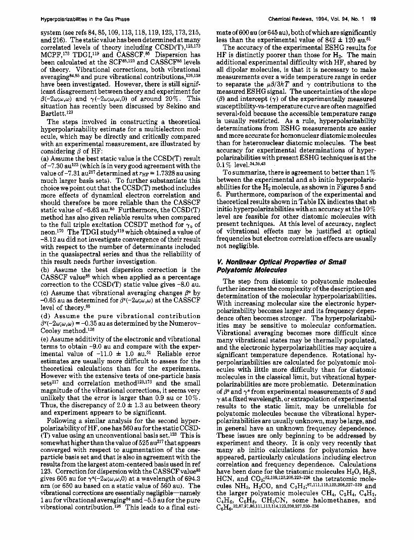
Figure 1. Calculated dispersion curves are shown for y~ for several nonlinear optical processes for the H atom.l& bor comparison, the dotted line is the lowest order dispersion formula obtained by truncating eq 18 at the A V L ~ term. The y versus q.2 curves for all nonlinear optical processes must tend to the slope and intercept of the dotted line as v - 0. While no simple general relation exists once the curves begin to deviate from the dotted line, nevertheless, a single curve does accurately represent the dispersion curves for all the nonlinear optical processes as long as resonance is not too closely approached. The first resonance is at U L ~ = 68, 90, 102, and 136 X lo8 cm-2 for DFWM, THG, ESHG, and dc Kerr, respectively.

Table VI. The ab Initio Values of y(He) from the CI-Hylleraas Calculation of Bishop and Pipin’” Compared with the Results of Absolute Experimental Determinations.

~ ~~~~

experiment X (nm) ref Yexpt (au) y d C (au) dc Kerr 632.8 11 44.3 f 0 . 8 44.211 dc Kerr 514.5 19 47.3 h 3 44.771 dc Kerr 632.8 30 53.6 f 4 44.211 dc Kerr 632.8 31 51.6 f 8 44.211 THG 1055 60 44.3 f 4 45.338 Theory and experiment agree to within the stated experi-

mental uncertainty except for one dc Kerr measurement. The best test is at the 2% level of accuracy. The values of y d c include the reduced mass correction.

where higher terms in eq 18 cannot be neglected and y has increased to twice its static value. At U L ~ = 20 X 108 cm-2, near the top of the usual experimental frequency range, the dispersion curves for dc Kerr, DFWM, ESHG, and THG in Figure 1 differ by no more than 0.7 9%.

The simplest atom for which a comparison between theory and experiment is possible is the He atom. Methods special to the two-electron problem (i.e. CI- Hylleraas) have been applied by Bishop and co- workerslmJsZ to compute the frequency dependence of y for He, and the accuracy of their final ab initio resultslm is thought to be better than 0.1 % . The ab initio results for He have been used to calibrate all of the most accurate gas-phase hyperpolarizability measurements. Absolute experimental determinations of y(He) from dc Kerr effect and THG experiments, summarized in Table VI, are in agreement with the calculated results for He. However, the experimental


2.90 0

T I T T I I

1

I 1

10 20 30

( 1 Oacm-2) 2

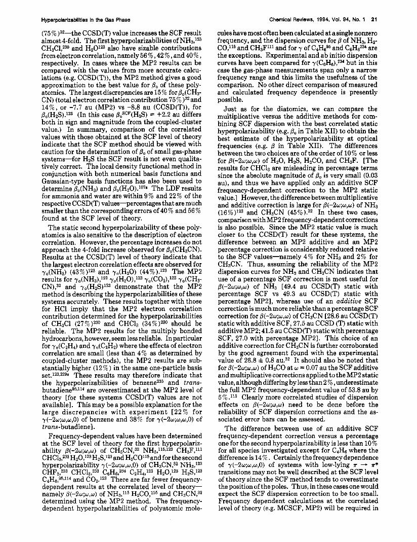
uL F igure 2. The ratio of the independent tensor components of y for the noble gas atoms is shown as a function of Y L ~ for ESHG. Kleinman symmetry is broken when yl1/yI deviates from the static limiting value of 3. The curve through the experimental pointa for He is from the ab initio calculation of Bishop and Pipin,l@J while the other curves are empirical fits of eq 20 to the experimental data: filled symbols, refs 37 and 47; open symbols, ref 58.

results for y are a t the 2-20% level of accuracy, and more accurate measurements are needed for a critical test of the ?(He) calculations. The experimental ESHG results for yZzZL/yZXXZ for He, shown in Figure 2, agree with theory at the 0.1 % level of accuracy. The ratios yZZzZ/yzXXZ have also been measured for Ne, Ar, Kr, and Xe, and those experimental results are also plotted in Figure 2. These experimental ESHG results show that the coefficient A’ in eq 20 is negative for He and Ne, near zero for Ar, and positive for Kr and Xe, but so far there are no ab initio results for A’ other than those for He with which to compare.

Table VI1 gives the coefficients that result from fitting eq 18 to the measured and calculated hyperpolarizabilities of the atoms H, He, Ne, Ar, Kr, and Xe. The

coefficients given for H and He are estimates of the leading coefficients of the infinite order power series expansion based on the limited ab initio results. For the other atoms, where the data is less accurate and extensive, both the ab initio and experimental results were fit by a truncated expansion keeping terms only up to B v L ~ . The fitted value of B so obtained will be somewhat sensitive to the frequency range of the data used in the fit, but the fitted value of A should be reliable.

Theoretical and experimental dispersion curves may be compared for Ne, Ar, and Kr, and the comparison shows that it is feasible to calculate y(-Bv;v,v,O) of multielectron atoms with quantitative accuracy. The discrepancy between the best t h e ~ r e t i c a l l ~ ~ J ~ ~ and e ~ p e r i m e n t ~ ” ~ ~ results is only 2-10% for static y of the noble gas atoms Ne, Ar, Kr, and Xe. It should also be noted that the hyperpolarizabilities of argon, krypton, and xenon are related experimentally since the hyperpolarizabilities of Kr and Xe are measured relative to y of argon. The theoretical ratios y(Kr)/y(Ar) and y(Xe)/y(Ar) which are both within 4% of the experimental ratios are closer than the absolute values would indicate. Another striking result of this comparison is that calculation and experiment are in good agreement for the dispersion coefficient A even when there are gross discrepancies for the static value of y. The calculated static y seems to be much more sensitive to the effects of the electron correlation treatment and basis set selection than is the frequency dispersion. Certainly for neon where the range of optical frequencies considered is far from the first resonance, the different theoretical methods, MP2, MCSCF, and SCF, give similar dispersion curves since the positioning of the poles, which will in general be too high at the SCF and MP2 levels of theory, does not strongly affect the results. The fact that the dispersion coefficients A and B are similar at the SCF104J22 and at the best correlated levels of theory (MCSCF,lo4 MP2122) indicates that, for neon, a multiplicative correction for the frequency dependence in combination with the best static value will give the most reliable theoretical values for y(-2v;v,v,O) and y(-v;O,O,v) of neon. The MP2 dispersion curve,

Table VII. Comparison of the Results of Theoretical Calculations and Experimental Measurements for the Frequency Dependence of y for ESHG in Atoms.

Y0,Calc .&IC Beak Cdc Yo.expt ‘ $ x P t Bexpt atom (au) (10-lO cm2) ( W0 cm4) (1030 cm6) (au) (10- cm2) (10-20 cm4) H 1 338.216b 2.020 633 2.932 5 3.73 He 43.145‘ 0.455 0 0.145 8 0.060 4 Ne l l O d 0.498 0.230 lose 0.513 0.237

99r 0.529 0.256 86.58 0.478 0.22 68.7h 0.473 0.203 68.8’ 0.472 0.200 5 4 0.466 0.19

Ar 122ok 1.076 1.373 1167‘ 1.066 2.033 Kr 2 810k 1.354 4.684 2 600‘ 1.389 3.465 Xe 7 020m 6 888‘ 1.499 8.048 The coefficients of the power series expansion of y in terms of Y L ~ given by eqs 18 and 19 have been fit to measured and calculated

values of y for frequencies up to Y L ~ = 6 9 = 30 X 108 cm-2. The experimental results for Ne, Ar, Kr, and Xe were calibrated using the ab initio He dispersion curve. Except in the case of Ne, where three electron-correlated and three SCF calculations are compared, all the calculations include electron correlation. The ab initio results given in this table include the reduced mass corrections. Reference 146, sturmian basis. c Reference 100, CI-Hylleraas (this dispersion curve is used for calibration of the ESHG experiments; note the misprint for C in SI units in Table I1 of ref 34). d MP2 dispersion curve of ref 122 with multiplicative correction using static CCSD(T) of ref 171. e Reference 33. f Reference 104, CASSCF. g Reference 103, MCTDHF. Reference 122, SCF. Reference 104, SCF. j Reference 178, SCF. MP2 dispersion curve of ref 122 with multiplicative correction using static CCSD(T) of ref 170. Reference 34. Reference 170, CCSD(T).

Hyperpolarlzabilities in the Gas Phase Chemical Reviews, 1994, Vol. 94, No. 1 13

140 I I I I

n

2 - ....

60 SCF I---- _ _ _ _ _ _ _ _ _ - - - -

40 / 0 10 20 30

( 1 o8 2

v L Figure 3. Theoretical and experimental dispersion curves are compared for y of the Ne atom (also see Table VII). The solid line is the experimental dispersion curve fit to the ESHG measurements indicated by the filled circles.33~" Other experimental measurements are indicated by open symbols (circles, ESHG;37959 triangles, THG;M@ diamond, dc Kerr30). The measurements indicated by the three open circles at the right37 have been shown to be invalid.% These measurements were responsible for the reported36 but now discredit- ed33J04J22.172 observation of anomalous dispersion for y of Ne. Theoretical dispersion curves calculated at several levels of theory are plotted SCF,1MJ22J78 MCTDHF,l03 CASSCF,l@ MP2,122 and CCSD(T).'22J70 (See Table VII.) The upper two SCF curves are indistinguishable in this plot, and are about 1 au below the Hartree-Fock limit. The best theoretical estimate of y is the curve marked CCSD(T), which is obtained by applying a multiplicative static CCSD(T) correction to the MP2 dispersion curve, as in eq 11. Remarkably robust results are obtained for the dispersion even though the value of static y varies by a factor of 2 for the various calculations.

adjusted with a multiplicative correction based on the CCSD(T) static value (see eq l l ) , is illustrated in Figure 3, together with the experimental measurements and dispersion curves calculated ,by other correlated and SCF methods.

Although we have been considering results for ESHG, it has been demonstrated that the dispersion coefficients fit to the results of ESHG calculations also describe the calculated results for other nonlinear optical processes in a given atom,100J46J87J92 When plotted versus uL2, experimental measurements of y are also seen to be consistent with a single dispersion curve, as illustrated for Ar in Figure 4. Such a plot of y versus Y L ~ appears to be a useful way of comparing y for different nonlinear optical processes. The theoretical dispersion curve for Ar (i.e. MP2 frequency dependence with multiplicative correction using the CCSD(T) static valuelZ2) lies slightly above and rises less steeply than the experimental dispersion curve. Since the MP2 method is likely to overestimate the frequency of the first resonance, one may expect that the frequency dependence at the MP2 level of theory will rise less steeply than observed experimentally and the B coefficient determined at the MP2 level of theory will be smaller than the one deduced from experiment.

1800

1600

n - : 1400

6

1200

1000

Ar -

l b I

I / I _ _ 0 10 20 30

2 VL ( l o8 Cm-2)

Figure 4. Experimental measurements of y for the Ar atom are compared. The solid curve is the experimental dispersion curve fit to the ESHG data indicated by the filled circles.MP@ Other measurements are indicated by open symbols (circle, ESHG;59 triangles, THG;W@ diamonds, dc Kerr;lgrO squares, CARS;72*73?75 inverted triangle, ac Ker9). When plotted versus Y L ~ as suggested by eqs 18 and 19, the results for all five nonlinear optical processes agree with a single dispersion curve. The dotted curve is the best theoretical estimate of y for ESHG in Ar (see Table VII, MP2 dispersion122 with multiplicative correction using static CCSD(T)171).

I V. Nonllnear Optical Propertles of Dlatomlc Molecules

Shifting consideration from atoms to diatomic molecules adds new features: (i) the molecule need not be centrosymmetric, so that ,6 is not forced to be zero by symmetry in all cases, (ii) there are more independent tensor components because of the lower symmetry, (iii) the molecule has a single vibrational degree of freedom, and (iv) the molecule has rotational degrees of freedom. The ,f3 or y tensors of a diatomic molecule may have as many as 4 or 10 independent components, respectively. Since gas-phase measurements are related to the isotropically averaged hyperpolarizability tensors, gas- phase experimental measurements can determine at most 2 or 3 independent combinations of tensor components, respectively. Much more information is needed to completely describe the hyperpolarizabilities of diatomic molecules than is the case for atoms, more information than can be provided even in principle by gas-phase experiments. Just as in the case of atoms, a wider range of diatomic molecules have been studied by ab initio calculations than by experiment. The molecules and molecular ions for which there are ab initio calculations of hyperpolarizabilities include: Hz+ (refs 140-143 and 194-196), H:! (refs 113 and 197-206), Liz (ref 207), N2 (refs 95,123,167, and 208-210), F2 (ref 211), Clz and Brp (ref 861, LiH (refs 119 and 212), BH and CH+ (ref 213), OH, OH+, and OH- (refs 173,183, and 214), HF (refs 84, 85, 109, 113, 118, 119, 123, 173, 196, and 215-217), HC1 (ref 218) and CO (refs 114 and 123). There are measurements only for Hz, Dz, Nz, 0 2

(refs 11-14, 19, 26, 29,38,47, 48, 50, 52, 53, 60,64,66, 68, and 73-75), HF and HC1 (ref El), and CO and NO (ref 53).


The dispersion of the electronic hyperpolarizabilities of molecules follows the same dispersion relations (eqs 18-22) as apply in the case of a t o m ~ , ' ~ ~ J ~ ~ but the frequency-dependent vibrational and rotational hyperpolarizabilities for different nonlinear optical processes are not related by such simple expressions as eqs 18-22 for the electronic hyperpolarizabilities. However, for homonuclear diatomic molecules, p' = 0 and the expressions for yv are relatively simple even in the dynamic case. Taking the high-temperature limit of the full quantum expression and ignoring the J dependence of agu and Aagu give6J34

y{( -Wg;Wl,WZ,W3) = ci{2ai, + (8/45)Aai,] {(I - x1Zu)-l + (1 - x13J1 + (1 - (23)

and

Y ~ ( - w , w ~ , w ~ , w ~ ) = C/2O1,2,(1- ~ l 2 ~ ) - ~ ( h ~ ~ ~ ) - ~ + c:(8/45)Aaiu{-2(1 - x12u)-1 + 3(1 - x13u)-1 +

31 - x23u)-11(hWgu)-1 (24) where

xlzu = (a1 + W 2 ) 2 / ( o g , ) 2 (25) In the static limit these expressions reduce to just

Shelton and Rice

terms containing p ~ u p u u ( h u g u ) - 2 , pgupuuagu( hogu)-2, and p~,(p~, - i ~ ~ , ) ( h w ~ , ) - ~ have been neglected in eqs 28 and 30.

The expressions for the rotational hyperpolarizability of a homonuclear diatomic molecule for the dc Kerr effect and ESHG, in the high-temperature limit and ignoring the J dependence of Aa, are simple and instructive. The result for dc Kerr a t optical frequencies is

In the case of THG or ESHG, where optical frequencies are far above vibrational resonances, the vibrational contributions to the total hyperpolarizability will be small, negative and vary as v - ~ . The vibrational contributions are larger in the static limit and for the ac and dc Kerr effects and DFWM, and in the case of CARS the vibrational contribution becomes dominant when the optical field frequency difference is tuned near a Raman resonance.

For a heteronuclear diatomic molecule the expressions for p' and yv contain additional terms. Only the expressions for the dc Kerr effect and ESHG will be given here. Keeping the leading terms, and again taking the high-temperature limit and ignoring the J dependence of molecular properties, one gets

for the dc Kerr effect, and

for ESHG, where x = (w /wgJ2 . Terms containing piupuu(hwgu)-2 have been neglected in eqs 27 and 29, and

7; = (Aa2/15kT)[3 + (1 - xR)-'] (31)

while the result for ESHG a t optical frequencies is

7; = ( A ~ ~ ~ / 1 5 k T ) [ ( l - 4xR)-l + 2(1 -xR)-'] (32)

where XR = ( w / w R ) ~ and WR = 4B(kT/hB)1/2 is the root- mean-square rotational transition frequency for the rotor with rotational energy levels J ( J + 1)hB. Devi- ation from isotropy of the gas due to the redistribution of the population of the IJ,M) free rotor states for each value of J accounts for about l/4 of yR for the dc Kerr effect,132 but does not affect yR for ESHG. For processes such as dc Kerr, ac Kerr, and DFWM, where pairs of input frequencies sum to zero, yR at optical frequencies will be comparable to the static value and cannot be ignored, while for ESHG and THG the result at optical frequencies will be reduced by a typical factor (wR/0)2 = and will be negligible for most purposes. In the high-frequency limit, neglecting all terms such as (1 - X R ) - ~ in yR, one finds that yp for ac Kerr and DFWM are 2/3 and 8/9 as large as 7: for dc Kerr. In the static limit, 7: for the dc Kerr effect increases by a factor of 4/3 from its optical frequency value. The rotational hyperpolarizabilities of a general, polar molecule in the high-frequency, high-temperature limit have in fact already been given for the dc Kerr effect and ESHG. The rotational hyperpolarizabilities in this case are just the terms in addition to y in eqs 8 and 9.

For molecules such as HZ with widely spaced rotational levels, expressions taking explicit account of the individual rovibrational states are available5 and should be employed. These expressions have the same overall form as eqs 23-32, but they differ in that they (i) contain J-dependent numerical coefficients, (ii) include the J dependence of the molecular transition frequencies and polarizabilities, and (iii) sum over the distribution of initial states. Expressions for yv and yR for homonuclear diatomic molecules are

and

Hyperpolarlzabilities in the Gas Phase Chemical Reviews, 1994, Vol. 94, No. 1 15

R Y (-~,,;01,~2,03) = cJ(1/16)(J+ 1)(J+ 2)(2J+ 1)-1(2J+ 3)-1 x ( p ( J ) - ( 2 J + 1)(2J + 5)-'p(J + 2)) x

J(1/45)J(J + 1)(2J - 1)-'(2J + 3)-1 x (Aa J,J+~)~(~W,J,,J+~)-~~(UJ,~J+~) +

( ~ a j , j ) (k W ~ F ( U J , U J ) (34) where p(u,J) is the normalized population distribution function, and

F,(uJ,U'J') = -2G(W1+W2,WUj,,tj,) + 3G(W1+W3,WUj,,'~~) + ~G(W~+W~,W,J,,~J~) (38)

and

G(w,D) = 11- (w/D)~I- ' (39) Either Ell, Fil or EL, FL are used according to whether yil or yI is desired. The expression for yR includes both the A J = f 2 rotational Raman contribution and the AJ = 0 contribution due to M sublevel population redistribution. For the A J = 0 terms of yR where D - 0, G(w,fl) = 1 if w = 0 and G = 0 otherwise. The frequency arguments for ( Y , J , ~ ~ J ~ and A ~ , J , , ~ J ~ have not been explicitly indicated in eqs 23-34 since they have not been rigorously established as yet. The derivation is most nearly complete for the dc Kerr effect where w appears in only a few of the denominators in eqs 13 and 14. For the dc Kerr effect one finds that ( A ~ J J ~ ) ~ is replaced by Aajjt(0) Ac~JJ~(o ) in yR.12 In other cases the replacement is ad hoc, where for example, ag, = agu(w) is chosen when evaluating yv for ESHG. Expressions similar to eqs 33 and 34 have also been derived for polar diatomic molecule^.^

The adequacy of the high-temperature limit of the quantum expressions for yv and yR given by eqs 33-39 has been investigated for H2+ and H2 by Bishop and Lam.131J94 For these molecules it is found that the high- temperature limit of yv is adequate except for molecules in higher vibrational states, but the high-temperature limit of yR gives poor results even for molecules in the u = 0 state.131 Where the high-temperature limit is adequate, for example for Na, the calculation of yVR at optical frequencies for homonuclear diatomic molecules is relatively straightforward. The single fundamental vibrational mode dominates, and the vibrational frequency and Raman transition polarizability are essentially the only required information. Table VI11 gives vibrational hyperpolarizabilities calculated for several diatomic molecules, while Table IX shows both theoretical and experimental results for Pe and ye for several diatomic molecules. Comparing Table VI11 and Table IX, one notes that in the static case pR and yVR are as large as or even much larger than p" and ye. A t optical frequencies, pR and yVR are usually just small correc-

Table VIII. Vibrational and Rotational Hyperpolarizabilities Calculated for Diatomic Molecules, at T = 295 K, Including Only the Fundamental Vibrational Transition.

dcKerr DFWM ESHG THG molecule static 632.8 nm 632.8 nm 694.3 nm 694.3 nm

P HF 6.36' 1.20b -0.35'

YV Hz+ 584' 388.87d -10.45d -3.43d H2 183.7' -7.2' 122f -13.5' -4.2" Dz 177.6' 0.3' 118' -6.4' -2.1' HF 49.1' 0.23b -5.5' -0.14' NZ 8lf 0.g 54f -1.u 02 118r 6.lf 78f -1.w -0.41

YR Hz+ 4157' H2 897' 6978 64oh -0.6h -0.2h Nz 6226' 4670' 4150' -0.11' -0.04l

"The values of p and y are given in atomic units. The yv results for dc Kerr tend to be anomalously small because of the cancellation of terms that occurs when evaluating YK = (3/2)(yi~ - yl). Quantum effects are significant for yR of Hz. The classical limit of eqs 34-39 gives 7:: = 909 au for dc Kerr and yR 834 au for DFWM at A = 632.8 nm, which are 30% larger tk: the results given by the full quantum calculation for Hz. b Reference 126, obtained using the classical orientational average of Nu- merov-Cooley results at w = 0.07 au ( u = 15363 cm-l); the result given here for dc Kerr is calculating using their tabulated tensor components. Reference 131, quantum expression applied for the u = 0 state (results up to u = 5 are given); the result for yv of Hz+ is consistent with the non-Born-Oppenheimer calculation of ref 142 which gives ynrrr = 2193 au; also, the classical orientational average for the u = 0 state gives the following: yv = 584 au and yR = 4576 au for Hz+; yev = 184 au and y R = 1169 au for Hz. Reference 195, classical orientational average for the u = 0 state; yv = 584.73 au in the static limit. e Reference 197. f Reference 134, with corrections given in ref 133. 8 Reference 12.

tions to p" and ye for diatomic molecules for ESHG and THG, but this is not the case for dc Kerr and DFWM. For this reason it is difficult to obtain reliable experimental results for De and ye from dc Kerr and DFWM measurements for molecules.

The best-studied diatomic molecule is H2. Experi- mental and ab initio results for ye of H2 are compared in Figure 5 and in Table X. The best measurements are at the 1% level of accuracy or better. The most accurate calculations are those of Bishop and co- w o r k e r ~ ~ ~ ~ and are also thought to be at the 1% level of accuracy or better. These calculations for H2 use explicitly correlated wave functions and include dispersion, vibrational averaging, and the vibrational hyperpolarizability. The electronic contribution smoothly increases with frequency, while the vibrational and rotational contributions to y show resonances at low frequencies. The tail of the fundamental vibrational resonance accounts for almost the entire vibrational contribution at visible optical wavelengths. The values of yv have been calculated and subtracted from the experimentally measured values of y to obtain the experimental estimates of ye in Figure 5. Experiment and theory agree very well for a variety of nonlinear optical processes. The agreement between the theoretical and experimental dispersion coefficients for ye of Hz and D2, shown in Table X, is as good as the agreement seen in Table VI1 for the inert gas atoms. The agreement among the recent experimental ESHG data for (y(HZ))/y(He) at infrared wavelengths,34earlier

Full quantum expressions. Classical limit.


Table IX. Comparison of a b Initio Calculations and Experimental Measurements of Hyperpolarizabilities for Diatomic Molecules”

Shelton and Rice

Pe (au) ye (au) ye or yeV (au) molecule v (cm-l) calc expt calc expt

Hz+ 0 0 0 (28)#rb Hz 0 0 0 (682.7)rc 686 f 4#yd D2 0 0 0 (663. l ) # s c 669 f 4#vd

Nz 0 0 0 10 1 O#,f 917 i 5#td 0 2 0 0 0 962 f 6#vd F2 0 0 0 512g Clz 0 0 0 (4750)h Brz 0 0 0 (9810)h LiH 0 -87W BH 0 55.1*J 12428*j CH+ 0 -12.4*J 344*J OH+ 0 (-8.61*)k (139*)k OH 0 (-13.43*)k (630*Ik OH- 0 (-35*)k

Liz 0 0 0 8-23 x 105e

NeH+ 0 -2.8*J 24*J HF 14 399 (-8.65)#,m -11.0 f 1.0” (651)tJ” 842 f 120” HC1 14 399 -8.34t.O -9.9 f 1.2” 4370#.” 4175 f 180”

1730 f 509 co 14 399 27 .O#,p 30.2 f 3.29 190W~P NO 14 399 34.3 f 3.99 2830 f 84q

Where possible, electronic hyperpolarizabilities are compared in the static limit. The calculations include electron correlations, except those marked with an asterisk (*). Averaging ye(R) over the unperturbed ground vibrational wave function is considered to be part of the calculation of ye, and such vibrationally averaged results for calculated ye are enclosed in parentheses. Vibrational averaging is distinct from the vibrational hyperpolarizability yv given in Table VIII. The results of ESHG measurements at h = 1319-457.9 nm for Hz, Dz, Nz, and 02 have been extrapolated to the static limit after subtracting calculated values of y v . However, only ESHG measurements a t h = 694.3 nm (v = 14399 cm-l) are available for HF, HCl, CO, and NO, so the calculated and measured results are compared for ESHG at this wavelength for these four molecules (yv has not been subtracted from these experimental measurements). Calculations or measurements where the hyperpolarizability has been determined at more than one frequency are marked with a number sign (#). Hz+: references 131 and 194; ye vibrationally averaged for u = 0 state; y e is much smaller than yv (see Table VIII). Hz, Dz: reference 197. Hz, Dz, Nz, 02: reference 34; experimental static ye. See also the following: for Ha, dc Kerr refs 11-14, 19, 29, ESHG refs 38, 47, 50, 52, and 53, THG ref 64, ac Kerr ref 66, and CARS refs 74 and 75; for Dz, dc Kerr refs 13, 19, and 29, ESHG refs 47 and 50, CARS refs 73 and 75; for Nz, dc Kerr refs 19 and 26, ESHG refs 47, 48, 52, and 53, THG refs 60 and 64, ac Kerr ref 68, CARS refs 72, 73, and 75; for Oz, dc Kerr ref 19, ESHG refs 47, 48, and 53, CARS refs 73 and 75. e Liz: reference 207, static SDTQ-MP4; also, static MP2, ye = 8.55 X lo5; and static SCF, ye = 10.07 X lO5*. f Nz: reference 123, static CCSD(T); also, static MP2, ye = 930; static SCF, ye = 730 using 15s 3p 2d] basis; ESHG at 694.3 nm from static CCSD(T) with SCF percentage dispersion gives ye = 1100, which may be compared with 1058 from the experimental dispersion curve of Table X or 1042 f 12 from the experiment of ref 53 scaled to new ?(He) of ref 100. See also the following: reference 95, SCF dispersion curve. Reference 209, static SDQ-MP4, ye = 830; static MP2, ye = 860; static SCF, ye = 665* using [6s 4p 3d lfl basis (more complete than ref 123). Reference 210, static SCF, ye = 766*. Reference 208, static SCF, ye = 700*. g Fz: reference 211, static SDQ-MP4; also, static MP2, ye = 541; static SCF, ye = 268*. Clz, Brz: reference 86, static SDQ-MP4 with vibrational averaging; also, static MP2, ye(Clz) = (5 050), ye(Brz) = (10 360); static SCF, ye(C1z) = (3 700*), ye!Brz) = (7 660*); pure vibrational hyperpolarizability, yv(Clz).= (930), yv(Brz) = (2 030). I LiH: reference 119, static TDGI P, dispersion results for 0-0.05 au for Pockels effect. See also the following: reference 212, static MCSCF, p” = -848, aPe/aR = -894; static SCF, pe = -410*, aPelaR = -426*. j BH, CH+: reference 213, static SCF. k OH+, OH, OH- : reference 214, static numerical SCF with vibrational averaging; pure vibrational hyperpolarizabilities: $(OH+) = (25.59), ?‘(OH+) = (458), $(OH) = (-6.71), ?‘(OH) = (275), $(OH-) = (-20). See also the following: ref 183, for OH-, static SCF, p” = -118*, ye = 94699*. NeH+: reference 183, static SCF. m HF: ESHG P e and ye at 694.3 nm from static CCSD(T) of ref 123 with CASSCF percentage dispersion of ref 85, and an additive -0.65 au vibrational averaging correction for p” from 694.3 nm CASSCF results of ref 85 and an additive 1 au vibrational averaging correction for ye from ref 84 (see text). See also the following: reference 123, static CCSD(T), p = -7.30, y = 560; static MP2, p” = -6.96, ye = 560; static SCF, p” = -5.38*, ye = 320*; ESHG 694.3 nm SCF, @e = -5.85*, ye = 359*. Reference 85, static CASSCF 6331, p” = -6.63; static SCF, Pe = -5.63*, ye = 323*; static CASSCF 4220, De = -6.49, ye = 444; ESHG 694.3 nm CASSCF, p” = (-7.8) (vibrational average), ye = 512. Reference 173, static CCSD(T), Pe = -7.18, ye = 509; static MCPF, p” = -7.23, ye = 514; static SCF, p” = -5.55*, ye = 298*. Reference 119, static TDGI, p” = -8.12; static SCF, p” = -5.83*; ESHG 694.3 nm TDGI, p” = -8.99 (dispersion based on A coefficient determined for Pockels effect). Reference 118, static SCF, p” = -5.62*, ye = 303*; ESHG 694.3 nm SCF, p” = -6.11*, ye = 340*. Reference 107a, static LDF p” = -8.6 (numerical), -7.8 (Gaussian). HF, HC1: reference 51, experimental ESHG Dev and yeV at 694.3 nm rescaled to new y(He) of ref 100. HCl: reference 218, ESHG p” and ye at 694.3 nm from static CCSD(T) with MP2 percentage dispersion; also, static CCSD(T), p” = -7.23, y e = 3446; static MP2, p” = -8.09, ye = 3493; static SCF, = -3.72*, ye = 2726*. p CO: reference 123, ESHG p” and ye at 694.3 nm from static CCSD(T) with SCF percentage dispersion; also, static CCSD(T), Pe = 23.5, ye = 1590; static MP2, p” = 22.6, ye = 1500; static SCF, p” = 21.1*, y e = 1020*. See also the following: reference 107a, static LDFp” = +26.7 (numerical), +31.5 (Gaussian). CO, NO: reference 53, experimental ESHG Pev and yev at 694.3 nm rescaled to new y(He) of ref 100.

experimentalESHG data for ( y(Hz))/ ( y(D2)) at visible wavelength^,^^ and the corresponding calculated re- sultslg7 is at the 0.1% level. However, one may raise Some questions about the significance of the 0.1 %J

possible systematic errors have been assessed. Since the experimental results are obtained at finite gas density, intermolecular interactions are a possible problem. Recent work indicates that these effects are at the 0.1% level in the measurements for H2.35 A

second problem is that the expression for yv in terms of the dynamic transition polarizabilities auuf(v), where Y is the laser frequency, is not exact. For ESHG, a rough bound on the systematic uncertainty in y v follows

unknown effective frequency at which auu’ should be evaluated. For the infrared ESHG measurements for Hz this bound gives a maximum uncertainty of *6?6 (about fl au) for when v* = Y is chosen, although

agreement for (r(H2))/7(He) until several sources of from < a;,,(y*) < a;u,(2v), where v* is the

Hyperpolarlzabillties in the Gas Phase 17

1200 1 H2

1000 c i T

0 10 20 30

( lo8 Cm-2) 2

wL Figure 5. Experimental measurements of ye for the hydrogen molecule are compared with theoretical dispersion curves. The experimental values of ye are obtained from the directly measured values of yevR by subtracting the calculated values of yvR. (See eqs 33-39 and Table VIII.) The theoretical results for ye are from the ab initio calculations of Bishop et al.lg7 The solid curve, which is the ab initio result for ye for ESHG,lg7 is seen to agree very well with the filled circles, which are ESHG measurements of ye.34,50 Other measurements of ye are indicated by open symbols (circle, ESHG;s3 triangle, THG;U diamonds, dc Kerr;11-14J9,29 squares, CARS,73,74 Rado’s value75 as reevaluated by Lundeen et al.73 is off scale; inverted triangle, ac Kerr66). The measurements of ye for all five nonlinear optical processes are consistent with a single dispersion curve. The dotted curve shows the ab initio result for yevR for ESHG in H2 and gives an indication of how the frequency dependence of ye and yVRdiffers. Since yVRvanishes as v-2 at high optical frequencies, whereas ye slowly increases with V L ~ , the solid and dotted curves converge in the high frequency limit. The resonance in the dotted curve is due to vibrational overtone transitions at about 8075 cm-l.

Table X. Comparison of the Results of Theoretical Calculations and Experimental Measurements of the Frequency Dependence of the Electronic Hyperpolarizabilities r“ for ESHG for Hz, Dz, N2, and 0 2 .

Hz 683b 1.286 1.81 686c 1.200 2.25

Nz l0lW 0.974 0.87 917c 1.003 1.85 02 963c 1.112 4.60

a These are the only diatomic molecules for which there are experimental dispersion curves. The coefficients of the power series expansion of ye in terms of V L ~ given by eqs 18 and 19 truncated at the BvL term have been fit to the measured and calculated values of ye for frequencies up to Y L ~ = 6vz = 30 X los cm-2. Calculated values of yv were subtracted from the measured values of y to obtain the experimental values of ye. b Reference 197. Reference 34. From static CCSD(T) of ref 123 and SCF dispersion curve of ref 95.

D2 664b 1.268 1.73 669c 1.184 2.10

the actual error is thought to be much smaller. The ratios of tensor components y1l/yL measured by ESHG tend to fall below Bishop’s calculated results, as shown in Figure 6. The discrepancy is only marginal, about 0.2% for the best measurements, but it may indicate an inadequacy of the experiments or the calculations of ye or yVR. The ratio q / y I is sensitive to yVR, because in the high-frequency limit yiR/ylR = 9. Rotational

Chemical Reviews, 1994, Vol. 94, No. 1

3.00 i

0 10 20 30

( lo8 2

u L Figure 6. The ratio of the independent tensor components of (7) for the hydrogen molecule is shown as a function of vL2 for ESHG. The filled38147 and open53 circles are the experimental measurements of yll/yI for H2. The solid curve is the ratio f l y ? determined by the ab initio calculations of Bishop et al.,lg7 while the dotted curve is the ratio of just the electronic contributions, y ; / ~ \ , also determined by the same calculation. The discrepancies between theory (solid curve) and experiment (filled circles) are at the 0.2% level. The solid and dotted curves diverge at low frequencies since the frequency dependence of y e and yv is quite different and both contributions are large. A t high frequencies the curves converge since there yv vanishes as r2.

hyperpolarizabilities and overtone vibrational hyperpolarizabilities are not accounted for in Bishop’s calculation of y1l/yI. Accurate fundamental and overtone transition polarizabilities required for the calculation of yVR have been recently measured and calculated for H2 and D2.219-222

The other diatomic species for which calculations of p and y that include the effects of electron correlation have been reported are listed in Table IX, namel~Li2,~O~

HC1,218 and C0.114J23 Few calculations have been reported for the hyperpolarizabilities of ions’SCF calculations have been reported for CH+,213 OH+ and OH-,214 and NeH+.183 As yet, no experimental measurements are available for hyperpolarizabilities of charged species. Hyperpolarizabilities of negative ions are also notoriously difficult to calculate due to the need for very large diffuse basis sets and due to the problems associated with numerical finite difference procedures when determining values which are large in absolute magnitude. (There is a trade-off between the use of very small finite fields and obtaining sufficient numerical precision in the energy when using high- order finite difference te~hniques.21~)

As illustrated by the footnotes to Table IX, the effects of electron correlation on the properties can be substantial. For example, electron correlation increases po(LiH) by more than 100 % ,212 and Po(HC1) by 49 % .218 The smallest increase observed is 10% for p0(CO).123 It should be noted that some of these values are small in absolute magnitude and a small absolute change can result in a large percentage change [e.g. PoSCF(HCl) = 3.7 au and ~occsD(T)(HC1) = 7.2 au].218 However, in the

N2,95,123,209 F2,211 C12,86 Br2,86 LiH 119,212 HF 85,119,123,173 7 7


case of LiH, the change is considerable both in absolute and percentage terms [PoSCF(LiH) = -410 au and POMCSCF(LiH) = -848 aul .212 Electron correlation also increases the majority of the y values reported in Table IX, the exception being Liz where the SDQ-MP4 result is 22 70 smaller than the SCF value.207 Of the diatomic y values listed in Table IX, electron correlation has the largest effect (48 % ) on y(F2) and the smallest effect on r(C12) and y(Br2), where the increase is only 7% and 3 % , respectively.@

It is useful to assess the adequacy of the MP2 method for predicting P and y of these diatomics since the MP2 method is one of the cheapest methods for including the effects of electron correlation and is therefore practical for the study of the hyperpolarizabilities of the larger systems where methods such as CCSD(T) become intractable. (Density functional theory is also worth investigating but to date few calculations of hyperpolarizabilities have been reported.) For P,(HF), P,(HCl), and pO(CO) where MP2 results are available, the method is seen to perform well, giving values within 5 % , lZ3 12% ,218 and 4% 123 of the best correlated results. The MP2 method is also reliable for predicting y for the diatomics investigated. The largest difference is 8% of yeo(Nz) where the total electron correlation contribution is 28% .lZ3 Thus, these results, just as those for the hyperpolarizabilities of the noble gas a t ~ m s , ' ~ ~ J ~ ~ demonstrate that second-order perturbation theory (MP2) can be useful for the study of electron correlation effects on hyperpolarizabilities even when these effects are considerable. There have been few local density functional results reported to date for 0, of small molecules. Results are available for p,(CO) and P,(HF), calculated using both numerical basis functions and Gaussian-type basis functions. The results for HF are within 18% (numerical) and 7% (Gaussian) of the CCSD(T) value-an improvement over the SCF error of 26%. The LDF values for po(CO) where the SCF error is only 10% are not as good: the LDF results overestimate the CCSD(T) value of 23.5 aulZ3 by 8.0 au (numerical) and 4.2 au (Gaussian), respectively.

Frequency-dependent @(-2w;w,w) values have been calculated for HF,85J23 HC1,218 and C0114J23 at a wavelength of 694.3 nm in order to compare with experimental SHG value^.^^^^^ As mentioned above, the choice of an additive or multiplicative correction is still being investigated. In the case of fl(-2w;w,w) for HF the difference between additive and multiplicative corrections to the SCF dispersion curve is only 2.5% of the total value of P ( - ~ W ; W , ~ ) . ~ ~ ~ By using the results of CASSCF dispersion calculations@ in conjunction with the CCSD(T) static value of -7.30 au,lZ3 the difference between additive and multiplicative corrections is even smaller (Le. 0.1 au or around 1 %). For @(-2w;w,w) for HC1 the difference between using the CCSD(T) static value to make an additive or a multiplicative correction to the SCF dispersion curve is about 5 % , but this is reduced to just 2 % when corrections are applied to the MP2 dispersion curve instead.218 Analysis of the frequency-dependent calculations for y(-2w;w,w,O) for N2,lZ3 HF,85J23 HC1,218 and C0114J23 at a wavelength of 694.3 nm also shows similar behavior, with the largest difference of 5 % between use of an additive and a multiplicative correction occurring for y(-2w;w,w,O) of CO.

Shelton and Rice

The fact that the additive and multiplicative corrections are so close gives confidence that use of the SCF method for estimating the dispersion of 0 and y for these diatomic molecules is reliable. (For these systems there is also the obvious advantage that the frequency of the experimental measurement is far from a resonance.) If anything, the multiplicative correction may be slightly favored since in the cases where the dispersion correction has been determined using higher level methods [e.g. CASSCF for /3(-2w;w,w) and y(-2w;w,w,O) of HF;85 MP2 for @(-2w;w,w) and y(-2o;w,w,O) of HC1;218 MP2 and CASSCF for y(-2w;w,w,O) of the noble gas the multiplicative corrections are in closer agreement than the additive corrections. However, since the differences being discussed are on the order of a few percent, they are too small to make definitive conclusions about the best choice of method.

Full vibrational corrections to the hyperpolarizabilities have only been reported for a few of the many- electron diatomic molecules listed. The effects of vibrational averaging are less than 1.1 % for y,(Clz) and yo(Br2),86 less than 9% for P(HF),84985 and less than 1 % for Y ( H F ) . ~ ~ The results of numerical SCF calculations indicate that vibrational averaging has a slightly larger effectonP,(OH+) (13% ),&,(OH) (12%), ro(OH+) (8%), and yo(OH) (8% ).214 However, the pure vibrational contribution as estimated by the perturbation theory formalism is considerably larger for these static hyperpolarizabilities. The results for yO(Clz) and yo(Brz) illustrate that these large contributions are also sensitive to the treatment of electron correlation. For example, yv constitutes 39% of the total SDQ-MP4 yzizz value, whereas a t the SCF level the corresponding percentage is 63% .86 For Po(OH+), po(OH), and po(OH-) the pure vibrational contribution dominates the electronic contribution, e.g. po(OH+) changes sign and magnitude from 0; = -8.6 to py = +16.9 au, and yo(OH+) and yo(OH) also show substantial increases (4-fold for OH+).214 For HF, the pure vibrational contribution to the static first hyperpolarizability is also sizable (+6.78 au) although the vibrational contribution to the second hyperpolarizability is less than 10% .lZ6 The pure vibrational contributions to @(-2w;w,w) and y(-2w;w,o,O) of HF at w = 0.07 au (Y = 15363 cm-l) are considerably smaller than the corresponding contributions in the static limit and the results of more exact methods [-0.35 au for P(-Bw;w,w), -5.54 au for y(-2w;w,w,O)l are in good agreement with those determined from perturbation theory.lZ6 These frequency-dependent results substantiate the expectation that calculations of /3 and y a t optical frequencies which neglect vibrational effects should approach experiment to within 10%. The results of a comparison of ESHG experimental measurements, with calculations for N2, HC1, and CO neglecting vibrational effects, are consistent with this expectation. The differences between experiment and theory are 7% for y(N2),34J23 16% for P(HCl), and 5 % for y(HCl),51,218 11% for P(CO), and 10% for y(C0),53J23 which is very promising given the neglect of vibrational effects and the 1-1594 uncertainties in the experimental measurements.

The situation for HF, however, is somewhat different. The hyperpolarizabilities of hydrogen fluoride are probably the most widely studied of any many-electron

Hyperpolarirabtlities in the Gas Phase

system (see refs 84,85,109,113,118,119,123,173,215, and 216). The static value has been determined at many correlated levels of theory including CCSD(T) ,123J73

MCPF,173 TDGI,llg and CASSCF.85 Dispersion has been calculated at the SCFa5JZ3 and CASSCFa5 levels of theory. Vibrational corrections, both vibrational a ~ e r a g i n g ~ ~ * ~ and pure vibrational contributions,lz6JZ8 have been investigated. However, there is still significant disagreement between theory and experiment for p(-20;0,0) and y(-20;0,w,O) of around 20%. This situation has recently been discussed by Sekino and Bartlett.lZ3

The steps involved in constructing a theoretical hyperpolarizability estimate for a multielectron molecule, which may be directly and critically compared with an experimental measurement, are illustrated by considering p of HF: (a) Assume the best static value is the CCSD(T) result of -7.30 adz3 (which is in very good agreement with the value of -7.31 au217 determined a t FHF = 1.7328 au using much larger basis sets). To further substantiate this choice we point out that the CCSD(T) method includes more effects of dynamical electron correlation and should therefore be more reliable than the CASSCF static value of -6.63 au.85 Furthermore, the CCSD(T) method has also given reliable results when compared to the full triple excitation CCSDT method for yo of neon.170 The TDGI studyllg which obtained a value of -8.12 au did not investigate convergence of their result with respect to the number of determinants included in the quasispectral series and thus the reliability of this result needs further investigation. (b) Assume the best dispersion correction is the CASSCF valuea5 which when applied as a percentage correction to the CCSD(T) static value gives -8.0 au. (c) Assume that vibrational averaging changes p" by -0.65 au as determined for p"(-2w;w,w) at the CASSCF level of theory.85 (d) Assume the pure vibrational contribution P(-20;w,o) = -0.35 au as determined by the Numerov- Cooley method.lZ6 (e) Assume additivity of the electronic and vibrational terms to obtain -9.0 au and compare with the experimental value of -11.0 f 1.0 au.51 Reliable error estimates are usually more difficult to assess for the theoretical calculations than for the experiments. However with the extensive tests of one-particle basis sets217 and correlation and the small magnitude of the vibrational corrections, it seems very unlikely that the error is larger than 0.9 au or 10%. Thus, the discrepancy of 2.0 f 1.3 au between theory and experiment appears to be significant.

Following a similar analysis for the second hyperpolarizability of HF, one has 560 au for the static CCSD- (T) value using an unconventional basis set.123 This is somewhat higher than the value of 525 au217 that appears converged with respect to augmentation of the one- particle basis set and that is also in agreement with the results from the largest atom-centered basis used in ref 123. Correction for dispersion with the CASSCF values5 gives 605 au for ye(-2w;w,w,0) a t a wavelength of 694.3 nm (or 650 au based on a static value of 560 au). The vibrational corrections are essentially negligible-namely 1 au for vibrational averaginga4 and -5.5 au for the pure vibrational contribution.lZ6 This leads to a final esti-

Chemical Reviews, 1994, Voi. 94, No. 1 10

mate of 600 au (or 645 au), both of which are significantly less than the experimental value of 842 f 120 au.5l

The accuracy of the experimental ESHG results for HF is distinctly poorer than those for H2. The main additional experimental difficulty with HF, shared by all dipolar molecules, is that it is necessary to make measurements over a wide temperature range in order to separate the ppf3kT and y contributions to the measured ESHG signal. The uncertainties of the slope (p) and intercept (y) of the experimentally measured susceptibility-vs-temperature curve are often magnified several-fold because the accessible temperature range is usually restricted. As a rule, hyperpolarizability determinations from ESHG measurements are easier and more accurate for homonuclear diatomic molecules than for heteronuclear diatomic molecules. The best accuracy for experimental determinations of hyperpolarizabilities with present ESHG techniques is a t the 0.1 % le~e1.3~J69~3 .

To summarize, there is agreement to better than 1 % between the experimental and ab initio hyperpolarizabilities for the H2 molecule, as shown in Figures 5 and 6. Furthermore, comparison of the experimental and theoretical results shown in Table IX indicates that ab initio hyperpolarizabilities with an accuracy at the 10% level are feasible for other diatomic molecules with present techniques. At this level of accuracy, neglect of vibrational effects may be justified a t optical frequencies but electron correlation effects are usually not negligible.

V. Nonllnear Optical Propertles of Small Polyatomlc Molecules

The step from diatomic to polyatomic molecules further increases the complexity of the description and determination of the molecular hyperpolarizabilities. With increasing molecular size the electronic hyperpolarizability becomes larger and its frequency dependence often becomes stronger. The hyperpolarizabilities may be sensitive to molecular conformation. Vibrational averaging becomes more difficult since many vibrational states may be thermally populated, and the electronic hyperpolarizabilities may acquire a significant temperature dependence. Rotational hyperpolarizabilities are calculated for polyatomic molecules with little more difficulty than for diatomic molecules in the classical limit, but vibrational hyperpolarizabilities are more problematic. Determination of p" and ye from experimental measurements of p and y at a fixed wavelength, or extrapolation of experimental results to the static limit, may be unreliable for polyatomic molecules because the vibrational hyperpolarizabilities are usually unknown, may be large, and in general have an unknown frequency dependence. These issues are only beginning to be addressed by experiment and theory. It is only very recently that many ab initio calculations for polyatomics have appeared, particularly calculations including electron correlation and frequency dependence. Calculations have been done for the triatomic molecules H20, HzS, HCN, and C0~;32~10g~123~20a~22~226 the tetratomic mole-

the larger polyatomic molecules CHI, C2H4, C4H2, C4H6, C6H8, CH&N, some halomethanes, and

cules NH3, H&O, and C2H2;87,111,115,123,208,227-229 and

C6H6~32,87,91,95,111,113,114,123,208,227,230-236


Table XI. Vibrational Hyperpolarizabilities Calculated at the MP2 Level for Polyatomic Molecules (from ref 124). molecule static dcKerr DFWM ESHG THG

Shelton and Rice

P NH3 76.3 4.76 -0.18 Hz0 1.47 3.31 -0.21

YV coz 540 -21.5 272 -81 0.48 NH3 1754 135 305 -18.0 -5.9 HzO 235 10.3 137 -10.9 -2.6

0 All values of and yv are for w = 0.07 au (v = 15363 cm-1) and T = 295 K, and are given in atomic units.

The vibrational hyperpolarizabilities of polyatomic molecules are difficult to calculate. All of the cy2, pp, p2a, pap, and p4 type terms which can contribute for diatomic molecules also contribute to P,yv for polyatomic molecules (see eqs 15 and 16). The added difficulty is that there are very many vibrational modes for a polyatomic molecule and there are cancellations between the individual vibrational mode contributions. The results of early attempts at evaluating yv for polyatomic molecules are probably unreliable because none of these calculations had complete and accurate data for the required molecular parameters, and none of these calculations systematically evaluated all terms up to a given 0rder.~0p~~J30J~8 Recently, expressions in a form suitable for calculation have been derived by Bishop and Kirtman,l2"lZ7 and applied to calculate p' and yv for several polyatomic molecules.124 These calculations confirm that the contributions of P and yv can be significant and that reliable estimates require careful systematic calculation. These calculations also indicate that the effect of vibrational averaging on the value of p" is ~ m a l l . ' ~ ~ J ~ ~ Results of these recent calculations of vibrational hyperpolarizabilities for polyatomic molecules are shown in Table XI, and may be compared to results for electronic hyperpolarizabilities given in Table XII. The static values of P and yv are comparable to the electronic hyperpolarizabilities. At optical frequencies P and yv are much smaller, with the vibrational hyperpolarizabilities smallest for THG, as expected. For ESHG, the vibrational contribution to /3 is <2% for H2O and NH3, while the vibrational contribution to y is about 6% for COz but <1% for HzO and NH3. This is consistent with previous work where yv was found to be small for molecules such as CH4 with high vibrational frequencies and larger for molecules such as CF4 with lower vibrational frequen- ~ i e s . ' ~ ~ A possible experimental strategy for determining the vibrational hyperpolarizabilities is to compare the dispersion curves for several nonlinear optical processes for the same molecule. A t high optical frequencies the vibrational contributions either become negligible or tend to a constant value, whereas the electronic contributions follow a common dispersion curve. This allows the vibrational and electronic terms to be disentangled in favorable cases using high-quality measurements over a wide wavelength range for several nonlinear optical processes. Several attempts along these lines have been p ~ b l i s h e d , ~ J ~ J ~ ~ but no definitive study yet exists because the required systematic and accurate experimental data is not available.

Table XI1 gives the hyperpolarizabilities of polyatomic molecules for which gas-phase hyperpolariz-

4000 1 CH4 T A

- I 3

2000 0 1 10 20 30

2 UL ( l o 8 Cm-2)

Figure 7. Experimental measurements of yevR for the CHI molecule are compared. The solid curve is eq 18 fit to the ESHG data indicated by the filled circles,34?43 with the X = 1319 nm point excluded from the fit. The true dispersion curve may turn down sharply at low frequency due to y v R , as is suggested by the dispersion curve for y of Hz in Figure 5, but the frequency dependence of yVR for CHI is presently unknown. Other measurements are indicated by open symbols (circles, ESHG;52*55 triangle, THG;62 diamonds, dc Kerr;22s28 square, CARS73). The static SCF result from Table XII, ye = 1870 a ~ , 2 ~ 7 falls off scale. One expects that yevR versus Y L ~ will follow a different dispersion curve for each nonlinear optical process even though ye versus Y L ~ may be described by a single dispersion curve. Comparison of the dispersion curves for yevR would allow one to obtain an experimental estimate of yvR. The present measurements appear to be consistent with a single dispersion curve, which seems to indicate that y v R is small compared to y e for CHI.

ability measurements have been done. Many molecules have been measured using the dc Kerr effect, but except in special cases, the uncertainties of the dc Kerr hyperpolarizabilities are of order *lOO%. The most extensive and reliable data comes from ESHG measurements, with dispersion curves available for eight

C&, and mC4H10). For the five molecules where there is a pair of independent ESHG measurements at the same wavelength for comparison, the average experimental error bar is k1.376 and the independent measurements tend to agree to within their joint uncertainty (reduced x2 = 1.3). For this reason we will consider ESHG results almost exclusively in the sub- sequent discussion. Figure 7 compares the dc Kerr, ESHG, THG, and CARS experimental results for y(CH4).

Hyperpolarizabilities have been calculated using ab initio methods for many of the molecules listed in Table XII. All the calculations shown there include the effects of electron correlation in the static limit, except those for HCN,32,208 CHF3,232$233 and CH4.227 The absolute magnitudes of all the 0, and yo values listed increases with electron correlation, except for Po of HzCO which decreases by 7% at the MP2 level of t h e ~ r y . ~ ~ ' J ' ~ As observed for the diatomics, the effects of electron correlation can also be substantial for the hyperpolarizabilities of polyatomics. In particular, Po(CH3CN) is dominated by the electron correlation contribution

polyatomic molecules (c02, CH4, CF4, SF6, C&, C&,

Hyperpolarlzabllities in the Gas Phase

(75%)32-the CCSD(T) value increases the SCF result almost 4-fold. The first hyperpolarizabilities of NH3,123 CH3C1,230 and H20123 also have sizable contributions from electron correlation, namely 56 % ,42 % , and 40 % , respectively. In cases where the MP2 results can be compared with the values from more accurate calculations (e.g. CCSD(T)), the MP2 method gives a good approximation to the best value for Po of these polyatomics. The largest discrepancies are 15 % for p0(CH3- CN) (total electron correlation contribution 75 % )32 and 14%, or -7.7 au (MP2) vs -8.8 au (CCSD(T)), for p0(H2S).123 (In this case PoSCF(H2S) = +2.2 au differs both in sign and magnitude from the coupled-cluster value.) In summary, comparison of the correlated values with those obtained at the SCF level of theory indicate that the SCF method should be viewed with caution for the determination of Po of small gas-phase systems-for H2S the SCF result is not even qualita- tively correct. The local density functional method in conjunction with both numerical basis functions and Gaussian-type basis functions has also been used to determine P0(NH3) and ,80(H20).107* The LDF results for ammonia and water are within 9% and 22 % of the respective CCSD(T) values-percentages that are much smaller than the corresponding errors of 40 % and 56 % found at the SCF level of theory.

The static second hyperpolarizability of these polyatomics is also sensitive to the description of electron correlation. However, the percentage increases do not approach the 4-fold increase observed for P0(CH3CN). Results at the CCSD(T) level of theory indicate that the largest electron correlation effects are observed for yo(NH3) (43%)123 and y0(H20) (44%).123 The MP2 results for yo(NH3),123 yo(H20),123 y0(C02),123 yo(CH3- CN),32 and 70(H2S)123 demonstrate that the MP2 method is describing the hyperpolarizabilities of these systems accurately. These results together with those for HC1 imply that the MP2 electron correlation contribution determined for the hyperpolarizabilities of CH3C1 (27%)230 and CHCl3 (34%)230 should be reliable. The MP2 results for the multiply bonded hydrocarbons, however, seem less reliable. In particular for yo(C2H4) and yo(C2H2) where the effects of electron correlation are small (less than 4% as determined by coupled-cluster methods), the MP2 results are sub- stantially higher (12%) in the same one-particle basis et.^^^,^^^^ These results may therefore indicate that the hyperpolarizabilities of benzene235 and trans- butadieneg5J14 are overestimated at the MP2 level of theory [for these systems CCSD(T) values are not available]. This may be a possible explanation for the large discrepancies with experiment [22 % for 7(-2o;w,o,O) of benzene and 38% for y(-2w;w,w,O) of trans-butadiene] .

Frequency-dependent values have been determined at the SCF level of theory for the first hyperpolarizability @(-2w;w,w) of CH3CN,32 NH3,115J23 CH3F,ll1 CHC13,233 H20,123 H2S,123 and H2COl15 and for the second hyperpolarizability 7(-2w;w,w,O) of C H S C N , ~ ~ NH3,123

C4H6,95J14 and C02.123 There are far fewer frequency- dependent results at the correlated level of theory- namely P(-Bw;o,o) of NH3,115 H2C0,115 and CH3CN,32 determined using the MP2 method. The frequency- dependent hyperpolarizabilities of polyatomic mole-

CHF3,233 CHC13,233 C6H6,234 C2H4,123 H20,123 H2S,123

Chemlcal Reviews, 1994, Vol. 94, No. 1 21

cules have most often been calculated at a single nonzero frequency, and the dispersion curves for P of NH3, H2- C0,115 and CH3F111 and for y of C4H695 and C,3H6234 are the exceptions. Experimental and ab initio dispersion curves have been compared for y(C6H6),234 but in this case the gas-phase measurements span only a narrow frequency range and this limits the usefulness of the comparison. No other direct comparison of measured and calculated frequency dependence is presently possible.

Just as for the diatomics, we can compare the multiplicative versus the additive methods for com- bining SCF dispersion with the best correlated static hyperpolarizability (e.g. Po in Table XII) to obtain the best estimate of the hyperpolarizability a t optical frequencies (e.g. P in Table XII). The differences between the two choices are of the order of 10% or less for p(-2w;w,w) of H20, H2S, H2C0, and CH3F. [The results for CHCl3 are misleading in percentage terms since the absolute magnitude of Po is very small (0.03 au), and thus we have applied only an additive SCF frequency-dependent correction to the MP2 static value.] However, the difference between multiplicative and additive correction is large for P(-20;w,u) of NH3 (16%)123 and CH3CN (45%).32 In these two cases, comparison with MP2 frequency-dependent corrections is also possible. Since the MP2 static value is much closer to the CCSD(T) result for these systems, the difference between an MP2 additive and an MP2 percentage correction is considerably reduced relative to the SCF values-namely 4% for NH3 and 2% for CH3CN. Thus, assuming the reliability of the MP2 dispersion curves for NH3 and CH3CN indicates that use of a percentage SCF correction is most useful for p(-2w;w,w) of NH3 [49.4 au CCSD(T) static with percentage SCF vs 49.3 au CCSD(T) static with percentage MP21, whereas use of an additive SCF correction is much more reliable than a percentage SCF correction for P(-20;0,w) of CH3CN [28.6 au CCSD(T) static with additive SCF, 27.5 au CCSD (T) static with additive MP2; 41.5 au CCSD(T) static with percentage SCF, 27.0 with percentage MP21. This choice of an additive correction for CH3CN is further corroborated by the good agreement found with the experimental value of 26.8 f 0.8 au.32 It should also be noted that for @(-2w;w,w) of H2CO at w = 0.07 au the SCF additive and multiplicative corrections applied to the MP2 static value, although differing by less than 2 % ,underestimate the full MP2 frequency-dependent value of 53.8 au by 5% .l15 Clearly more correlated studies of dispersion effects on p(-2w;w,w) need to be done before the reliability of SCF dispersion corrections and the associated error bars can be assessed.

The difference between use of an additive SCF frequency-dependent correction versus a percentage one for the second hyperpolarizability is less than 10% for all species investigated except for C4H6 where the difference is 14 % . Certainly the frequency dependence of y(-20;0,w,O) of systems with low-lying ?r - ?r*

transitions may not be well described at the SCF level of theory since the SCF method tends to overestimate the position of the poles. Thus, in these cases one would expect the SCF dispersion correction to be too small. Frequency dependent calculations at the correlated level of theory (e.g. MCSCF, MP2) will be required in


Table XII. Measured and Calculated Values of (a) B and (b) 7 for Small Polyatomic Molecules.

Shelton and Rice

a. /3 Values

ahc (au) @Lc (au) E:,, (au) E P t (au) m o 1 e c u 1 e StatlC ESHG 694.3 nm dc Kerr 632.8 nm ESHG 694.3 nm

HCN

NH3 CHsCN CH3F

CH3Cl CFaC1 CF3Br CHzFz CHzClz CFzClz CHF3

CHC13 CFCls

Linear -6.85*,b

-34.3' 24.2O

-40.38

15Bk

-17.2*pn

0.03*

-18.P -7.7q

-40.4*

Axial -49.1'

-46.3@8 -59 f 31h 27.5"~~

-31 f 125'

-18.4*~"

-1.4"

Other -21.1p -8.W

-53.8"'

b. y Values

-12.8 & 3.1h 125 f 156'

84 f 31h

-156 f 125'

-19 f 9'

-16 f 47t

94 f 187y -280 f 130" -250 f 130"

-48.9 f 1.2d

-57.0 f 4.2' -58.2 f 1.2@j

-69.2 f 2.8'

-42.1 f 1.9' 4.0 f 2.3"

-60.3 f 1.9" -25.2 f 0.9' -27.8 f 0.6@J

1.2 f 2.6" -30.9 f 9.6"

26.3 f 0.8@J

13.3 f 1.4"

-140 f 9'

-22.0 f 0.9d -10.1 f 2.ld

-35.0 f 2.1d -67.1 f 1.2d

7Lc (au) yLC (au) r:$ (au) C P t (au) Y:$ (au) c p t (au) molecule static ESHG 694.3 nm dcKerr 632.8 nm ESHG 694.3 nm THG 694.3 nm CARS 532 nm

1870*vw

1816*sb 5310"

1 2140ee 115Off

4200' 4240'

5420k

780*J'

10310"

2040Oij

661OCc 1572P' 130Off

560OC 5660@ye

878*?"

13160"

292W.j

Spherical 2887 f 140" 3079 f 160@aa 1491 f 80" 1241 f 77"'

19730 f 640' 17800 f lWn 2338 f 19ijbb 1908 f 133""

Linear

20400 f 4300dd

2005 f 51388

114 i o x 103 ii Axial

8020 f 16Wdd 12800 f 640@' 6400 f 6400" 8000 f 3200"

11 f 11 x 103 11

3257 f 16#J 3164 f 36" 1133 f 6#J 1095 f 36'

16480 f 240"

1565 f 8#J 1564 f 24d

1368 f 7#J 1346 f 15d

6147 f l l O d 4619 f 370@J 2875 f 23@ 2617 f 257"j 6860 f 360" 3680 f 160' 7520 f 520' 1853 f 130'

11070 f 360" 7340 f 120" 1636 f 72' 1771 f 80@J

13470 * 360" 11550 f 360"

23900 f 480#*& 24780 f 600""

3997 f 12oV

1200 f 6oV

1793 f lloV

1890 f 28ph

3125 f 12oV

2544 f BY.

1914 f 7 2

3930 f 60W

13580 f 200W

2100 f 32W

1823 f 27W

6075 f 9 W

8340 f 13W


Table XI1 (Continued)


~

b. y Values

molecule static ESHG 694.3 nm dcKerr 632.8 nm ESHG 694.3 nm THG 694.3 nm CARS 532 nm yLc (au) yHc (au) C P t (flu) C P t (au) C P t (au) Cpt (au)

Other HzO 180OP 220w 2311 f 120d 2360 f 600"" HzS 7900s 117009 10300 f 260d so2 480 f 800t CH30H 4586 f 130d (CH3)zO 6300 f 130d CZH4 67OOo0 1 0 2 0 0 ~ ~ -600 f 4000dd 9120 f 205"" CZH6 3850 f 800dd 6365 f 32#J C3He 11700 f 290OPp 10740 f 54#+ 10200 f 2900"" C4H6 2290099 383009s 27700 f 1600""

n-C4H10 15100 f 260OPp 13730 f 7WJ 12700 f 3300nn C6H8 38000*sm 88000*pm 90600 f 8400""

a The calculated values are p" and ye, while the experimental values are P.. and yeV at optical frequencies. None of the calculations includes vibrational averaging. Where an experimental dispersion curve has been measured, this is indicated by #. The calculations include electron correlation, except those marked with *. Results at a wavelength different that stated in the column heading are indicated by @. The experimental values calibrated against He have been rescaled using the calculated y(He) values from Bishop and Pipin." * HCN: reference 32, static SCF and y. See also the following: reference 208, static SCF, p = -7.95*, y = 1740*. NH3: reference 123, static CCSD(T) p and y, ESHG at 694.3 nm from CCSD(T) static p and y with SCF percentage dispersion; also, static MP2, @ = -32.5, y = 4100; static SCF, p = -15.1*, y = 2400*. See also the following: reference 227, static SDQ-MP4, @ = -30.5, y = 3864; static MP2, p = -33.8, y = 4256; static SCF, p = -16.5*, y = 2503*; static best estimate, p = -34.9, y. = 4175. Reference 115, static MP2, p = -29.7; static SCF, p = -14.3; MP2 and SCF /3 dispersion curves for ESHG and dc Kerr; basis set less complete than in ref 227. Reference 107a, static LDF, p" = -32.2 (numerical), -37.2 (Gaussian). SF.5, COz, NH3, Hz0, HzS, CHsOH, (CH3)zO: reference 53, ESHG rescaled. e CH3CN: reference 32, static CCSD(T) /3 and y, ESHG at 514.5 nm from CCSD(T) static @ with MP2 additive dispersion, and from CCSD(T) static y with SCF additive dispersion; also, static MP2, p = 27.8, y = 3870; static SCF, p = 6.1*, y = 3012*. f CH3CN: reference 32, ESHG at 514.5 nm, p and y. 8 CH3F: reference 111, static MP2 p, ESHG at w = 0.07 au from MP2 static @with SCF percentage dispersion; also, PK = -42.2, dc Kerr at w = 0.07 au from MP2 static j3 with SCF percentage dispersion; static SCF p = -36.2*. h CHBF, CHZFZ, CHF3 0, and CHI, CF4 y: reference 28, dc Kerr. i Halomethanes: reference 56, ESHG rescaled. j CHsF, CHF3: reference 52, ESHG at 514.5 nm, p and y, rescaled. CH3C1: reference 230, static MP2 @ and y; also, static SCF, B = +9.1*, y = 3951*. I Chloromethanes: reference 23, dc Kerr. CHF3: reference 233, static SCF 0 and y, dynamic SCF at 694.3 nm; also, dc Kerr at 694.3 nm, SCF, p = -17.3*, y = 811*, assuming Kleinman symmetry. See also the following: reference 232, static SCF, p = -17.4*, y = 792*. CHC13: reference 230, static MP2 @ and y, ESHG at 694.3 nm from static MP2 p with SCF additive dispersion from ref 233, and static MP2 y with SCF percentage dispersion from ref 233; also, static SCF, /3 = -0.05*, y = 6830*. See also the following: reference 232, static SCF, @ = -0.1*,. y = 6683* with (7s7p4d I 6s5p3d 1492~) basis set. Reference 233, static SCF, p = -8.8*, y = 6245* with (6s4p2d I3s2p2d I3slp) basis set, and dynamic SCF at 694.3 nm. p H20: reference 123, static CCSD(T) p and y, ESHG at 694.3 nm from CCSD(T) static p and y with SCF percentage dispersion; also, static MP2, p = -17.5, y = 1780; static SCF, p = -10.8*, y = 1010*. See also the following: reference 223, static SDQ-MP4, /3 = -16.8, y = 1628; static MP2, = -17.3, y = 1748; static SCF, p = -11.0*, y = 992*. Reference 107a, static LDF, p" = -21.8 (numerical), -19.6 (Gaussian). HzS: reference 123, static CCSD(T) and y, ESHG at 694.3 nm from CCSD(T) static p and y with SCF percentage dispersion; also, static MP2, (3 = -8.8, y = 7800; static SCF, HzS: reference 20, dc Kerr. a H2CO: reference 115, static MP2 @, ESHG at w = 0.07 au at MP2 level; also, static SCF, p = -43.2*; MP2 and SCF dispersion curves for ESHG and dc Kerr. SOz: reference 15, dc Kerr. CsHbF, C6HF5: reference 16, dc Kerr p. CHI: reference 227, static SCF y. CH4, CF4, SF6, COz, CZH6, C3H8, n-C4Hlo: reference 34, ESHG y at 694.3 nm from ESHG dispersion curves with measurements over 1319-457.9 nm, except for C4H6 which is a single measurement at 1064 nm. y Fluoromethanes: reference 62, THG rescaled. CH4, Cc4, SF6, COz, CH3C1, CFzClZ: reference 73, CARS with vibrational contributions of cy2 type subtracted. O0 CH4, CF4, C(CH3)4, SF6: reference 22, dc Kerr at 633 nm except CH4 at 458 nm. bb SF6: reference 30, dc Kerr. cc CzHz: reference 229a, static CCD y; ESHG at 694.3 nm from CCD static y with MCSCF y2222 percentage dispersion from ref 229c; also, static MP2, y = 5970; static SCF, y = 5400*. See also the following: reference 208, static SCF, y = 4471*. dd CzHz, C3H6, CzH4, CzHs: reference 26, dc Kerr. ee C4Hz: reference 229b, static SDQ-MP4 y; ESHG at 694.3 nm from SDQ-MP4 static y with MCSCF yslrr percentage dispersion from ref 229c; also, static MP2, y = 14,450; static SCF, y = 11,450*. See also the following: reference 208, static SCF, y = 9744*. ff Con: reference 123, static CCSD(T) y, ESHG at 694.3 nm from CCSD(T) static with SCF percentage dispersion; also, static MP2, y = 1170; static SCF, y = 800*, using [5s 3p 2d] basis; THG at 694.3 nm from CCSD(T) static with SCF percentage dispersion; THG, y = 1500. See also the following: reference 224, static SDQ-MP4, y = 1197; static MP2, y = 1251; static SCF, y = 844*; using [6s 4p 3d lfl basis (more complete than in ref 123). 88 COz: reference 18, dc Kerr. hh COz: reference 64, THG, rescaled. CSz: reference 27, dc Kerr. j j C6H6: reference 235, static MP2 y, ESHG at 694.3 nm from static MP2 with SCF percentage correction from ref 234; also, static SCF, y = 15240*. See also the following: reference 234, static SCF, y = 15220*, ESHG at 694.3 nm from SCF, y = 21780*. kk C6H6: reference 49, ESHG at 694.3 nm from dispersion curve, rescaled. C6H6, C&F3, CsF.5: reference 17, dc Kerr. mm CeH6, CzH4, C4H6: reference 54, ESHG, rescaled. nn HzO, C3H8, ?&4Hlo: reference 70, CARS. CzH4: reference 123, static CCSD(T) y, ESHG at 694.3 nm from CCSD(T) static y with SCF percentage dispersion; also, static MP2, y = 7500; static SCF, y = 6500*. See also the following: reference 231a, static SDQ-MP4, y = 6395; static MP2, y = 7507; static SCF, y = 6239*. pp C3H8, mC4Hlo: reference 25, dc Kerr.

C4H6: reference 95, static MP2 y, ESHG at 694.3 nm from MP2 static y with SCF percentage dispersion; also, static SCF, y = 14800*. See also the following: reference 231b, static SCF, y = 16800*; ESHG at 694.3 nm, y = 29300*; SCF dispersion curves for dc Kerr, DFWM, ESHG and THG. Reference 91, static SCF, y = 14846*. rr C6H8: reference 231b, static SCF y, dynamic SCF y at 694.3 nm; SCF dispersion curves for dc Kerr, DFWM, ESHG and THG. See also the following: reference 91, static SCF, y = 35118*.

20180 f 110@*

Halomethanes: reference 55, ESHG rescaled.

= +2.2*, y = 6000*.

(CH3)zO: reference 21, dc Kerr p.

order to investigate the reliability of SCF frequency- dependent corrections for y(-20;0,0,0) of these molecules.

We now compare the theoretical and experimental ESHG results for those systems where we have both an estimate of electron correlation effects on the static

value and a frequency-dependent correction at the appropriate wavelength. The agreement between the theoretical values (which neglect vibrational effects) and experiment for P ( - ~ W ; W , U ) of CHsCN, NH3, and HzO is very good with discrepancies of just 5 94, 1 % , and 4%, respectively. The differences for @(-%w;w,w)


of H2S (13%) and CH3F (19%) are somewhat larger but still reasonable. The agreement between theory and experiment for 0(-2w;w,w) of CHCl3 is good in terms of absolute values (-1.4 vs 1.2 f 2.6 a ~ ~ ~ ) especially considering that the frequency-dependent correction is determined in a one-particle basis set that gives a significantly different static SCF result (-8.8 au233) than found with a larger basis set (0.1 au232). For @(-2w;w,w) of NH3 and H20 it is possible to make a more complete comparison of theory with experiment since both vibrational averages and pure vibrational hyperpolarizabilities have been ca1c~lated. l~~ Assuming these vibrational effects are additive gives a best estimate for fl(-20;0,w) of H20 of (fixed nuclei value + vibrational averaging correction + pure vibrational contribution) = (-21.1 - 0.95 - 0.21) = -22.3 au and for @(-2w;w,w) of NH3 of (-49.3 + 2.3 - 0.2) = -47.2 au, which, since these vibrational corrections are small, still leaves both values in excellent agreement with experiment. As an overall measure of agreement for 0 of NH3, CHsCN, CH3F, H20, H2S, and CHC13, the average absolute value of the difference between theory and experiment is 8 % , not much larger than the average experimental error bar of f5% (reduced x 2 = 1.9).

Comparison between theory and experiment is not as good for y(-2w;w,w,O) of these polyatomic systems as for y(-2w;w,w,O) of the diatomics. Certainly from a theoretical point of view it quickly becomes more difficult to treat polyatomic systems to such high accuracy due to the cost associated with increasing basis set size (see Table 111). The best agreement is observed for y(-2w;w,w,O) of the smallest polyatomics (where the larger basis sets can be employed), NH3 (9% ), H2O (5 % ), and C02 (5%)-and in these three cases where the vibrational hyperpolarizability has also been calculated,lZ4 the best estimates of 5580,2190, and 1220 au are still in good agreement with the experimental values53 of 6147 f 1 1 0 , 2 3 1 1 f 120, and 1346 f 15 au, respectively. The calculated value for y(-2o;w,w,O) of CHCl3 is also in possibly fortuitously good agreement with experiment (2%) . The other y(-2w;w,w,O) values fall within 25% of experiment-C6H~ (24%), CH3CN (23% ), H2S (14%), and C2H4 (12%)-except for y(-2w;w,w,O) of C4H6 which, as mentioned earlier, overestimated the experimental value by 38%. For CH3CN it is likely that the majority of the error can be attributed to basis set incompleteness, particularly in the region of high order diffuse polarization functions. For C6H6 and C4H6 it seems most likely that the MP2 method is overes- timating the electron correlation contribution to the static value-this remains to be tested. To further substantiate this conclusion, it is interesting to note that use of the MP2 static value, rather than the CCSD- (T) one, results in a y(-20;0,w,O) of C2H4 which overestimates the experimental value by 25 % (compared to 1 2 % with the CCSD(T) value). As an overall measure of agreement for y of C02, NH3, CHsCN, C2H4, C4H6, C G H ~ , HzO, and H2S, the average of the absolute value of the difference between theory and experiment is 15 7 0 , distinctly larger than the average experimental error bar of f3% (reduced x2 = 37).

To summarize, current state-of-the-art calculations should be able to predict @(-2w;w,w) and y(-2w;w,w,O) of small polyatomic systems in the gas phase to within 10-20% ( p ) and to within 20-25% (y) of experiment

at optical frequencies. For larger polyatomic molecules and conjugated

molecules in particular, the electronic transition frequencies can be comparable to the optical frequencies involved in a nonlinear optical experiment. Near to resonance, the hyperpolarizabilities will have both real and imaginary parts, and the perturbation theory expressions are further complicated by the inclusion of phenomenological damping terms.6,s,237 The complex vibrationally resonant hyperpolarizabilities of molecules are well known from gas-phase CARS spectro- scopic studies.83 Electronically resonant hyperpolarizabilities have been employed for sum-wave-mixing in atomic gases,l and a wide range of resonant and multiply resonant nonlinear optical techniques have been applied to study molecules.238 However, there are few quantitative gas-phase measurements of the molecular hyperpolarizability near electronic resonance. Mea- surements of the real and imaginary parts of y for benzene, near an electronic resonance, were obtained from ESHG experiments at X = 514.5 nm with benzene vapor in various buffer An experimental method was demonstrated, although strong resonance effects were not observed in those experiments. The electronically resonant hyperpolarizabilities of molecular gases and the nonresonant hyperpolarizabilities of atoms and molecules in excited electronic states are largely unexplored.

V I , Relation to the Condensed Phase

Up to this point we have been considering isolated atoms and molecules. But, even gas-phase experiments are conducted at finite density. The usual prescription for treating the effect of the medium surrounding the molecule of interest is to introduce local field correction factors, most often of the Lorentz form, or to ignore the effect entirely. For the linear polarizability the Clau- sius-Mossotti relation in fact works rather we11.193~239 The situation may be different for nonlinear optics because the hyperpolarizabilities are sensitive to the outermost part of the molecular wave function, and the outermost wave function is most easily perturbed by neighboring molecules. There are two ways to assess the adequacy of the local field model. The first is to determine the gas-phase density dependence of the measured hyperpolarizabilities. The results will be density independent if local field factors correctly describe the situation. However, if intermolecular interactions change the molecular electronic structure, the measured hyperpolarizability will be density dependent and the coefficients of the virial expansion for the measured quantity will contain information about molecular pairs and larger clusters. Some calculations suggest that significant effects may be observed for atoms240 and small molecule^,^^^-^^^ and recent gas-phase ESHG experiments have observed significant density dependence for the measured hyperpolarizabilities of He, H2, N2, and Ar.35 In this regard it should be mentioned that the Kerr virial coefficients, routinely obtained in the extrapolation to zero density in gas- phase dc Kerr effect experiments, do not provide the desired information. There is indeed a strong density dependence in the dc Kerr effect which is not described by local field effects, but this is dominated by the binary and higher cluster polarizability anisotropy contribu-


tions. The desired cluster hyperpolarizabilities are buried and essentially unrecoverable.

The second way to assess the adequacy of local field factors is to compare hyperpolarizabilities, obtained from ab initio calculations, and gas- and liquid-phase measurements. A demonstration of this approach is the recent study of acet0nitrile.3~ One difficulty with this approach is that it may not be a simple matter to measure a given molecule in both gas and condensed phases, and the temperature range available in either the gas or liquid phase may be too restricted to allow the contributions from p and y to be separated. Another difficulty is that the absolute calibration of the liquid- phase measurements is rather uncertain. Almost all liquid-phase ESHG measurements are referred directly or indirectly to the SHG coefficient dll for quartz. Two values of dll differing by a factor of 0.6 have been obtained for quartz using different technique^.^^*^^^ Recent analysis by Robertsm concludes that the smaller value is the correct one to use, although most measurements reported in the literature to date have assumed the earlier value?" In the case of the CH&N study, the ab initio results were found to be in good agreement with the gas-phase results (differences of 5 76 and 23 % for p and y, respectively) but the liquid- phase results were larger by a factor of 2.3 or 3.5 depending on the choice of quartz reference value.32 This factor is distinct from the local field factors, already accounted for in the analysis of the experiment, which relate the externally applied field to the effective field inside the medium evaluated with the continuum approximation. This factor of 2.3 or 3.5 represents instead the modification of the molecule by explicit interactions with its immediate neighbors. Intermo- lecular interaction effects should be even larger for the conjugated molecules of interest for nonlinear optical applications, for example p-nitroaniline, and indeed p(-2w;w,w) for p-nitroaniline measured in solution differs by up to a factor of 2 in a range of solvents.247 Even in the least polar solvent (chloroform) the measured value of p(-20;w,w) for p-nitroaniline is still 2 or 3 times larger than the ab initio value including correlation (MP2) and dispersion (multiplicative SCF correction).lDpm Certainly the ab initio value was not calculated close to the one-particle or n-particle basis set limit, due to the size of the system. However, given the success of the MP2 method for the determination of the first hyperpolarizability of gas-phase systems as discussed above, it seems unlikely that this is the main reason for the discrepancy between theory and experiment. Rather this indicates that the solution effects on p(-2w;w,w) may be considerable. The strong intermolecular interaction effects seen in semiempirical calculations of /3 for p-nitroaniline molecular pa i rP2 are consistent with this conclusion.

In recent a reaction field in conjunction with ab initio methods has been used to study the hyperpolarizabilities of acetonitrile in the liquid phase. The results of these calculations indicate that the hyperpolarizabilities determined can be very sensitive to the choice of cavity radius. (A change of 0.05 nm in the spherical cavity radius can lead to a difference of a factor of 3 in the hyperpolarizability.) Results using an ellipsoidal cavity do not show such a marked dependence on the parameters of the cavity (factor of


Table XIII. Comparison of Static 811 Determined (without Vibrational Averaging) Using ab Initio and SemiemDirical Methods.

~~~~ ~

CNDO/ INDO/ molecule MNDO PM3 AM1 2b Sc ab initio LiH -438 -870 HF -8.1 -2.8 -8.9 -9.0 -15.6 -7.3 HCl -14.9 -0.3 -14.0 -7.2 co +1.3 -0.3 -4.1 -10.1 -10.7 +23.5 NH3 -10.3 -8.2 -11.2 -13.1 -18.7' -34.3 CH3F -32.6 -18.6 -37.6 -6.0 -46.8 -40.3 CH3C1 -45.7 -44.2 -36.2 +15.8 CH&N -2.1 -0.84 +1.1 +24.2 CHC13 -21.4 -12.5 -14.9 +0.03 HzO HzS

-11.3 -12.2 -13.0 +27.9 -21.0 -18.0 -7.7 -71.1 -55.0

-40.4 HzCO -48.5 -55.0 -53.5 a All ab initio results include electron correlation and are the

current best available values as reported in Tables 9 and 12. All values are given in atomic units. Reference 258. Reference 254. 811 quoted incorrectly in c.

1.4) and these results are closer to the experimental value based on the lower quartz reference.245 However, further work using more sophisticated solvation models is required in order to establish whether the reaction field model, with an appropriate choice of cavity parameters, can make reliable predictions for the hyperpolarizabilities of molecules in solution.

An adequate description of the response of a molecule in a condensed medium may require explicit accounting of the interactions between the nearest-neighbor molecules as they move and collide, resorting to the continuum approximation to describe the interactions with more distant molecules. A t long range where the molecular charge distributions do not overlap, the interaction may be treated as a perturbation. The classical interactions include dipole-induced-dipole, higher induced multipoles, field gradient, and nonlinear- induced polarizations and may be expressed in terms of the isolated molecule response tensors at real f r e q u e n ~ i e s . 9 ~ ~ ~ 9 ~ ~ ~ ~ Nonclassical contributions arise as a result of correlations between the fluctuating charge distributions on the interacting molecules and are closely related to the "dispersion" contribution to the intermolecular potential. These contributions may be expressed in terms of the response tensors for the isolated molecules a t imaginary f r e q u e n ~ i e s . ~ " ~ ~ ~ ~ ~ ~ ~ At short range where there is significant intermolecular electron overlap and exchange, a quantum calculation for the colliding molecular cluster is needed.249 These effects have been studied for the polarizability (ref 250 and references therein), but little is known about the importance of these effects for the hyperpolarizabilities. To summarize, the entire problem of interaction and solution effects on hyperpolarizabilities requires further theoretical and experimental study.

VZZ. Semiempirical versus ab Initio

Semiempirical methods are of interest because they are less expensive than ab initio methods, but the accuracy of hyperpolarizabilities obtained from semiempirical calculations has not been carefully tested. Here we will briefly assess the results of semiempirical methods used to calculate p. Table XI11 reports semiempirical values of Po for some of the diatomic and

26

polyatomic molecules listed in Tables IX and XI1 and compares the values with the best correlated static values reported in these tables. Since semiempirical methods include the results of experiment through the parametrization, it is appropriate to compare them with the best correlated values for these systems, which are within 10-20% of experiment.

The values determined with the MNDO, PM3, and AM1 semiempirical methods are obtained from finite field calculations of the energy.251 These methods have been parametrized for such gas-phase properties as ground-state geometries, dipole moments, and heats of formation,252 and in the case of MNDO for but not for the hyperpolarizabilities. The INDO/S parametrization used in the calculations reported by Parkinson and Zerner2b4 is specifically chosen to reproduce electronic spectra using the singly excited CI The INDO/S results are thus evaluated using the sum- over-states method. They also include additional polarization functions on hydrogen. Finally, comparison is also made to the results258 of finite field calculations using the CNDO/2 method which is based on the parametrization of Pople and Sega1.259

Even an initial glance a t Table XI11 indicates that the semiempirical results for PII can vary widely with respect to the ab initio values, both in sign and magnitude. For example, for CO the semiempirical methods predict the wrong sign for Po in all cases, except MNDO where the absolute value is much too small. Analysis of the components of the tensor indicate that the main error is in the prediction of P,,, which is calculated to be 6.6 au by the CCSD(T) method but ranges from -10.5 to -20.5 au with the semiempirical methods. The magnitude of Po for ammonia is considerably underestimated by the semiempirical methods. In this case it is the component along the dipole axis P,,, which is underestimated [from -0.4 au for MNDO to -15.2 au for CND0/2, compared to -39.6 au for CCSD(T)]. For Po of CH3C1 both components Pzzz and P,,, are incorrectly predicted using the semiempirical methods. For PLZZ7 the MP2 value is small (-1.1 au) whereas the semiempirical methods range from -23.9 au to -46.8 au, and for PLXX the semiempirical values are all large in magnitude but negative (-16.7 to -18.2 au) as compared to an MP2 value of +13.7 au. The MNDO, PM3, and AM1 results all indicate the first hyperpolarizability of CH3CN to be small in magnitude, contrary to the CCSD(T) and experimental values. This arises mainly from an underestimate of Pz,,, e.g. -19.0 au for MNDO as compared to the CCSD- (T) value of +2.8 au. The hyperpolarizability of CHCl3 is particularly sensitive to the method employed since it results from a near cancellation of P,,, with the sum of the P,,, and PzYy components. The semiempirical methods overestimate the magnitude of the PLZZ component at the expense of the other two components. Perhaps the largest error in terms of the absolute magnitude is observed for Po of H2S. A t the CCSD(T) level of theory the magnitude of all components is less than 10 au. The MNDO and PM3 methods however predict both the magnitude of the in-plane component Pzxx and the along axis component P,,, to be larger than 41 au. Lastly, as a cautionary note it is worth observing that although there appears to be reasonable agreement between MNDO, PM3, and AM1 results for Po of H20

Chemical Reviews, 1994, Vol. 94, No. 1 Shelton and Rice

and those from the CCSD(T) method, the MNDO, PM3, and AM1 methods all indicate that P,,, is larger in absolute magnitude than P2,,, the opposite to that determined from the CCSD(T) results.

In conclusion, these semiempirical methods, AM1, PM3, MNDO, and INDO/S, with the current parametrization are not reliable for either the quantitative or qualitative determination of Po for small gas-phase systems. However, as noted above, these methods, and AM1, MNDO, and PM3 in particular, have not been parametrized for higher order polarizabilities. It would be very useful to build up a database of ab initio data compiled from correlated results in order to improve the parametrization for Po and yo. High-level ab initio calculations also have the advantage that they can give information on all the tensor components rather than just PII which is the main quantity measured experimentally. Furthermore, values relevant to the static limit can be determined directly.

It should also be pointed out that one of the reasons it is so difficult to determine accurate Po values is that they often result from the trade-off between the different components, namely PEZZ (axial), P,,,, and Pzyy. For the larger “charge-transfer” molecules which are of interest experimentally since they exhibit large first hyperpolarizabilities (of the order of lo3 au or higher) the situation is different. In these cases ,811 is dominated by the along-axis component P,,,, the major part of which arises from the change in dipole moment between the ground and excited or “charge-transfer” state. The basis set requirement for the determination of P for such molecules is therefore reduced. In these cases, semiempirical methods such as MNDO, AM1, PM3, INDO/S, CNDO/VS have been found to give reliable trends across different donor or acceptor groups.2m,261 However, in these cases quantitative comparison with experiment is more difficult since the experimental measurements are generally made not in the gas phase, but in polar solvents.247

Semiempirical methods have also been applied to conjugated polymer^,^^^-^^^ which are of interest experimentally since they exhibit large second hyperpolarizabilities. There are no benchmark ab initio calculations or gas-phase measurements by which to assess the reliability of semiempirical calculations of y for long polymer chains, but the indications from ab initio calculations for the smallest polyenes95J14J23y231 and p ~ l y y n e s ~ ~ ~ are that electron correlation effects are small for y, so one may consider assessing semiempirical calculations by comparison with SCF calculations. The SCF results for C2H4, C4H6, and C6H8 are within 20 % of the gas-phase measurements when frequency dependence is taken into account. Comparing SCF resultsg1 for staticy of polyenes up to C22Hz4 with results of MNDO, AM1, and PM3 semiempirical calcula- tioq2G4 one finds that the SCF and semiempirical results agree within a factor of 4 for C4H6 and within a factor of 1.4 for the longer oligomers. The results of INDO-SDCI calculations for C4H6 and C6H8 agree with gas-phase measurements to within a factor of 1.6, but INDO-SCI calculations do not give even the correct sign for y.236 While not conclusive, this comparison suggests that reliable trends but not quantitative accuracy may be obtained from semiempirical calculations for conjugated polymers.


V I I I . Conclusion

The overall goal of this study has been to develop an understanding of and an ability to predict the nonlinear optical properties of materials. These aims have come closest to being fulfilled for atoms and diatomic molecules. In this case the interplay between gas-phase measurements and ab initio calculations has led to a sound quantitative understanding of the hyperpolarizabilities, including frequency dispersion, relations between tensor elements and the effects of electron correlation, and the vibration and rotation of the molecular frame, as described in sections I11 and IV of this review. General expressions which are computa- tionally tractable allow the frequency-dependent vibrational and rotational hyperpolarizabilities to be accurately calculated for arbitrary nonlinear optical processes, and a wide range of theoretical methods addressing the more difficult problem of calculating the (frequency dependent) electronic hyperpolarizability have been explored and refined. Accurate experimental determinations of the hyperpolarizabilities have been used to test the theoretical methods. Theoretical methods, validated by experiment, have then been turned to examine a wider range of systems, including open-shell atoms and ions which are inaccessible with present experimental techniques. Some broad trends are observed, but even for such small systems quantitatively accurate results require sophisticated and systematic calculation.

The methods successful for atoms and diatomic molecules have been extended with some success to the smallest polyatomic molecules. Accurate experimental measurements are available, although not very abun- dant. Methods for calculating the vibrational hyperpolarizabilities have been investigated but are not trivial and require more study. Ab initio calculations of the electronic hyperpolarizabilities employing large basis sets and including electron correlation are just becoming feasible with recently developed methods, and the accuracy of these ab initio calculations is beginning to approach the accuracy of the experimental measurements for the smallest polyatomic molecules. The effect of electron correlation is usually large. The accuracy of state of the art calculations is better than 10% for /3 and better than 25% for y at optical frequencies.

The extension of this program to larger polyatomic molecules confronts several outstanding problems. The computational cost of the present most accurate ab initio methods scales so rapidly with the size of the molecule that alternatives must be found. Less sophisticated methods are not quantitatively accurate but may give reliable trends when the hyperpolarizability is dominated by a single term (as in “charge- transfer” molecules such as p-nitroaniline), but for other systems even the trends may not be correct. Semiem- pirical methods as presently parametrized are unreliable. Direct tests of the calculations are often lacking since the molecules of interest for applications, such as p-nitroaniline and conjugated polymers, are not easily prepared in the gas phase for experimental study. Condensed-phase measurements are often available but are less directly related to the ab initio results. The indications are that the hyperpolarizabilities are very sensitive to the effects of intermolecular interactions, so the relation between the nonlinear optical response


of isolated molecules and the response of these molecules in the condensed phase is asubject which requires further study. In summary, the experimental and theoretical studies reviewed here have expanded the understanding of many aspects of molecular hyperpolarizabilities and have set the stage for attempts at accurate ab initio predictions of the nonlinear optical properties of practically useful materials.

References Hanna, D. C.; Yuratich, M. A,; Cotter, D. Nonlinear Optics ofFree A t o m and Molecules; Springer: Berlin, 1979. Bogaard, M. P.; Orr, B. J. In Int. Reu. Sci., Phys. Chem., Ser. 2, Vol. 2, Molecular Structure and Properties; Buckingham, A. D., Ed.; Butterworths: London, 1975; p 149. Bishop, D. M. Adu. Quant. Chem., in press. Special issue on molecular nonlinear optics: Int. J. Quant. Chem. 1992, 43, 1. Bishop, D. M. Reu. Mod. Phys. 1990,62,343. Boyd, R. W. Nonlinear Optics; Academic: San Diego, 1992. Butcher, P. N.; Cotter, D. The Elements of Nonlinear Optics; Cambridge University Press: Cambridge, 1990. Orr, B. J.; Ward, J. F. Mol. Phys. 1971, 20, 513. Buckingham, A. D. Adu. Chem. Phys. 1967,12, 107. Willetta, A,; Rice, J. E.; Burland, D. M.; Shelton, D. P. J. Chem. Phys. 1992, 97, 7590. Tammer, R.; Loblein, K.; Peting, K. H.; Huttner, W. Chem. Phys. 1992,168, 151. Shelton, D. P.; Rugar, B. Chem. Phys. Lett. 1993,201, 364. Carusotto, S.; Perrone, F.; Polacco, E. J. Chem. Phys. 1992, 97, 7979. Tammer, R.; Huttner, W. Chem. Phys. 1990,146, 155. Gentle, I. R.; Laver, D. R.; Ritchie, G. L. D. J. Phys. Chem. 1990, 94, 3434. Gentle, I. R.; Hesling, M. R.; Ritchie, G. L. D. J. Phys. Chem. 1990, 94, 1844. Gentle, I. R.; Ritchie, G. L. D. J. Phys. Chem. 1989, 93, 7740. Gentle, I. R.; Laver, D. R.; Ritchie, G. L. D. J. Phys. Chem. 1989, 93, 3035. Carusotto, S.; Iacopini, E.; Polacco, E. Nuouo Cimento 1985,5D, 328. Bogaard, M. P.; Buckingham, A. D.; Ritchie, G. L. D. Chem. Phys. Lett. 1982, 90, 183. Bogaard, M. P.; Buckingham, A. D.; Ritchie, G. L. D. J. Chem. SOC., Faraday Trans. 2 1981, 77, 1547. Dunmur, D. A.; Hunt, D. C.; Jessup, N. E. Mol.Phys. 1979,37,713. Bogaard, M. P.; Orr, B. J.; Buckingham, A. D.; Ritchie, G. L. D. J. Chem. SOC., Faraday Trans. 2 1978, 74, 1573. Burnham, A. K.; Buxton, L. W.; Flygare, W. H. J. Chem. Phys. 1977,67, 4990. Buckingham, A. D.; Sutter, H. J. Chem. Phys. 1976,64,364. Buckingham, A. D.; Bogaard, M. P.; Dunmur, D. A.; Hobbs, C. P.; Orr, B. J. Trans. Faraday SOC. 1970,66, 1548. Bogaard, M. P.; Orr, B. J.; Buckingham, A. D.; Ritchie, G. L. D. Mol. Phys. 1970, 18, 575. Buckingham, A. D.; Orr, B. J. Trans. Faraday SOC. 1969,65,673. Buckingham, A. D.; Orr, B. J. Proc. R. SOC. London A 1968,305, 259. Buckingham, A. D.; Dunmur, D. A. Trans. Faraday SOC. 1968,64, 1776. Boyle, L. L.; Buckingham, A. D.; Disch, R. L.; Dunmur, D. A. J. Chem. Phys. 1966,45,1318. Stiihelin, M.; Moylan, C. R.; Willetts, A.; Rice, J. E.; Shelton, D. P.; Donley, E. A. J. Chem. Phys. 1993,98, 5595. Shelton, D. P.; Donley, E. A. Chem. Phys. Lett. 1992, 195, 591. Shelton, D. P. Phys. Reu. A 1990, 42, 2578. Donley, E. A.; Shelton, D. P. Chem. Phys. Lett. 1993, 215, 156. Shelton, D. P. Phys. Reu. Lett. 1989, 62, 2660. Shelton, D. P.; Lu, Z. Phys. Reu. A 1988, 37, 3813. Shelton, D. P.; Lu, Z. Phys. Rev. A 1988, 37, 2231. Cameron, R. E.; Shelton, D. P. Chem. Phys. Lett. 1987,133, 520. Lu, Z.; Shelton, D. P. J. Chem. Phys. 1987, 87, 1967. Shelton, D. P. J. Chem. Phys. 1986,85, 4234. Shelton, D. P. J. Chem. Phys. 1986, 84, 404. Shelton, D. P. Phys. Reu. A 1986, 34, 304. Shelton, D. P. Chem. Phys. Lett. 1985, 121, 69. Pantinakis, A.; Dean, K. J.; Buckingham, A. D. Chem. Phys. Lett. 1985,120, 135. Shelton, D. P.; Mizrahi, V. Chem. Phys. Lett. 1985, 120, 318. Mizrahi, V.; Shelton, D. P. Phys. Rev. A 1985, 31, 3145. Mizrahi, V.; Shelton, D. P. Phys. Reu. Lett. 1985, 55, 696. Shelton, D. P. J. Opt. SOC. Am. B 1985,2, 1880. Mizrahi, V.; Shelton, D. P. Phys. Reu. A 1985,32, 3454. Dudley, J. W., 11; Ward, J. F. J. Chem. Phys. 1985, 82, 4673.

28 Chemical Revlews, 1994, Vol. 94, NO. 1 Shelton and Rice

(52) Shelton, D. P.; Buckingham, A. D. Phys. Reo. A 1982, 26, 2787. (53) Ward, J. F.; Miller, C. K. Phys. Rev. A 1979, 19, 826. (54) Ward, J. F.; Elliott, D. S. J. Chem. Phys. 1978, 69, 5438. (55) Miller, C. K.; Ward, J. F. Phys. Rev. A 1977, 16, 1179. (56) Ward, J. F.; Bigio, I. J. Phys; Reu. A 1975, 11, 60. (57) Finn, R. S.; Ward, J. F. J. Chem. Phys. 1974, 60, 454. (58) Bigio, I. J.; Ward, J. F. Phys. Reu. A 1974, 9, 35. (59) Finn, R. S.; Ward, J. F. Phys. Reo. Lett. 1971,26, 285. (60) Lehmeier, H. J.; Leupacher, W.; Penzkofer, A. Opt. Commun. 1985,

(61) Thalhammer, M.; Penzkofer, A. Appl. Phys. E 1983, 32, 137. (62) Ward, J. F.; Elliott, D. S. J. Chem. Phys. 1984, 80, 1003. (63) Young, J. F.; Bjorklund, G. C.; Kung, A. H.; Miles, R. B.; Harris,

(64) Ward, J. F.; New, G. H. C. Phys. Reu. 1969, 185, 57. (65) New, G. H. C.; Ward, J. F. Phys. Reu. Lett. 1967, 19, 556. (66) Rosasco, G. J.; Hurst, W. S. J. Opt. SOC. Am. E 1986, 3, 1251. (67) Rosasco, G. J.; Hurst, W. S. Proc. 1st Int. Laser Sci. Confer., Opt.

Sci. Eng. Ser. 6, No. 146; Lerner, R. G., Ed.; Am. Inst. Phys.: New York, 1986; p 261.

(68) Rosasco, G. J.; Hurst, W. S. Phys. Rev. A 1985, 32, 281. (69) Rosasco, G. J.; Hurst, W. S. J. Opt. SOC. Am. E 1985, 2, 1485. (70) Farrow, R. L.; Lucht, R. P.; Rahn, L. A. J. Opt. SOC. Am. E 1987,

4, 1241. (71) Farrow,R. L.;Lucht,R. P.Proc. TenthInt. Conf.RamanSpectrosc.;

Peticolas, W. L., Hudson, B., Eds.; University of Oregon: Eugene, 1986; p 15:27.

(72) Farrow, R. L.; Rahn, L. A. J. Opt. SOC. Am. E 1985,2, 903. (73) Lundeen, T.; Hou, S.-Y.; Nibler, J. W. J. Chem. Phys. 1983, 79,

(74) Hauchecorne, G.; Kerhervb, F.; Mayer, G. J. Phys. (Paris) 1971,32,

(75) Rado, W. G. Appl. Phys. Lett. 1967, 11, 123. (76) Pennington, D. M.; Henesian, M. A.; Hellwarth, R. W. Phys. Reu.

(77) Shimoji, Y.; Fay, A. T.; Chang, R. S. F.; Djeu, N. J. Opt. SOC. Am.

56, 67.

S. E. Phys. Rev. Lett. 1971, 27, 1551.

6301.

47.

A 1989,39, 3003.

B 1989,6, 1994.

Phvs. JETP 1979.49. 1033. (78) Vlasov, D. V.; Garaev, R. A.; Korobkin, V. V.; Serov, R. V. Sou.

(79) Miker, P. D. I n Physics of Quantum Electronics; Lax, B.,

(80) Altman, K.; Strey, G. J. Raman Spectrosc. 1982, 12, 1. (81) Shelton, D. P. Rev. Sci. Instrum. 1993,64,917. (82) Shelton, D. P.; Cameron, R. E. Rev. Sci. Instrum. 1988, 59, 430. (83) Levenson, M. D. Nonlinear Laser Spectroscopy; Academic: New

(84) Sekino, H.; Bartlett, R. J. J. Chem. Phys. 1986, 84, 2726. (85) Jaszuhski, M.; Jargensen, P.; Jensen, H. J. A. Chem. Phys. Lett.

Tannenwald, P. E., Eds.; McGraw-Hill: New York, 1966; p 60.

York, 1982.

1992,191, 293. (86) Archibong, E. F.; Thakkar, A. J. Chem. Phys. Lett. 1993,201,485. (87) Choura. P.; Carlacci, L.; King, H. F.; Prasad, P. N. J. Phys. Chem.

1989,93, 7120.

1158. (88) Sim, F.; Chin, S.; Dupuis, M.; Rice, J. E. J. Phys. Chem. 1993,97,

(89) Lizeretti, P.; Zanasi, R. J. Chem. Phys. 1981, 74, 5216. (90) Amos, R. D. Chem. Phys. Lett. 1986,124, 376. (91) Hurst, G. J. B.; Dupuis, M.; Clementi, E. J. Chem. Phys. 1988,89,

(92) Dykstra, C. E.; Jasien, P. G. Chem. Phys. Lett. 1984, 109, 388. (93) (a) Oddershede, J.; Jargensen, P.; Yeager, D. L. Comput. Phys.

Rep. 1984,2,33. (b) McWeeny, R. Int. J. Quantum Chem. 1983, 23, 405.

(94) Simandiras, E. D.; Amos, R. D.; Handy, N. C. Chem. Phys. 1987,

385.

114, 9. Sekino, H.; Bartlett, R. J. J. Chem. Phys. 1991, 94, 3665. Wormer, P. E. S.; Hettema, H. J. Chem. Phys. 1992, 97, 5592. Parkinson, W. A.; Zerner, M. C. Chem. Phys. Lett. 1987,139,563. Urban, M.; Noga, J.; Cole, S. J.; Bartlett, R. J. J. Chem. Phys. 1985, 83, 4041. Raghavachari, K.; Trucks, G. W.; Pople, J. A.; Head-Gordon, M. Chem. Phys. Lett. 1989,157, 479. Bishop, D. M.; Pipin, J. J. Chem. Phys. 1989, 91, 3549. Bishop, D. M.; RBrat, M. J. Chem. Phys. 1989,91, 5489. Koch, H.; Harrison, R. J. J. Chem. Phys. 1991,95,7479. Jaszufiski, M.; Yeager, D. L. Phys. Reo. A 1989,40, 1651. Jensen. H. J. A,; Jaraensen, P.: Hettema, H.; Olsen, J. Chem. Phys. Lett. 1991, 187; 387:

(105) (a) Senatore, G.; Subbaswamy, K. R. Phys. Reu. A 1987,35,2440. (b) Senatore, G.; Subbaswamy, K. R. Phys. Reu. A 1986,34,3619. (c) Subbaswamy, K. R.; Mahan, G. D. J. Chem. Phys. 1986,84, 3317.

(106) (a) Becke, A. D. Phys. Reu. A 1988, 38, 3098. (b) Perdew, J. P. Phys. Rev. E 1986,33,8822. (c) Lee, C.; Yang, W.; Parr, R. G . Phys. Reu. E 1988, 37,785.

(107) (a) Guan, J.; Duffy, P.; Carter, J. T.; Chong, D. P.; Casida, K. C.; Casida, M. E.; Wrinn, M. J. Chem.Phys. 1993,98,4753. (b) Colwell, S. M.; Murray, C. W.; Handy, N. C.; Amos, R. D. Chem. Phys. Lett. 1993, 210, 261.

(108) Voegel, T.; Hinze, J.; Tobin, F. J . Chem. Phys. 1979, 70, 1107. (109) Parkinson, W. A.; Oddershede, J. J . Chem. Phys. 1991,94, 7251.

(110) Taylor, P. R.; Lee, T. J.; Rice, J. E.; Almlbf, J. Chem. Phys. Lett. 1989,163, 359; (erratum) Chem. Phys. Lett. 1992,189, 197.

(111) Rice, J. E.; Amos, R. D.; Colwell, S. M.; Handy, N. C.; Sanz, J. J. Chem. Phys. 1990,93,8828.

(112) Karna, S. P.; Dupuis, M. J. Comput. Chem. 1991,12, 487. (113) Sekino, H.; Bartlett, R. J. J. Chem. Phys. 1986,85, 976. (114) Sekino, H.; Bartlett, R. J. Int. J. Quant. Chem. 1992,43, 119. (115) Rice, J. E.; Handy, N. C. Int. J. Quant. Chem. 1992, 43, 91. (116) Olsen. J.: Jsreensen. P. J. Chem. Phvs. 1985.82. 3235. (117j Hettema; H.;2ensen, H. J. A.; Jargeksen, P.f Oken, J. J. Chem.

(118) Aiga, F.; Sasagane, K.; Itoh, R. Chem. Phys. 1992,167, 277. (119) RBrat, M.; MBrawa, M.; Pouchan, C. Phys. Rev. A 1992,46,5471. (120) Koch, H.; Jamensen, P. J. Chem. Phvs. 1990, 93, 3333.

Phys. 1992, 97, 1174.

(121) Inoue, T.; Iwita, S. Chem. Phys. Lett. 1990,167,'566. (122) Rice, J. E. J. Chem. Phys. 1992, 96,7580. (123) Sekino, H.; Bartlett, R. J. J. Chem. Phys. 1993,98, 3022. (124) Bishop,D.M.;Kirtman,B.;Kurtz,H.A.;Rice, J.E. J. Chem.Phys.

1993,98, 8024. (125) Bishop, D. M.; Kirtman, B. J. Chem. Phys. 1992, 97,5255. (126) Bishou. D. M.; Kirtman. B. J. Chem. Phvs. 1991. 95. 2646. (127) Kirtman, B.; Bishop, D.'M. Chem. Phys.-Lett. 1990,'175, 601. (128) Malik, D. J. J. Chem. Phys. 1988,88, 2624. (129) Dykstra, C. E.; Malik, D. J. J. Chem. Phys. 1987,87, 2807. (130) Shelton, D. P.; Ulivi, L. J. Chem. Phys. 1988,89, 149. (131) Bishop, D. M.; Lam, B. Chem. Phys. Lett. 1988,143, 515. (132) Bishop, D. M.; Shelton, D. P. Phys. Reu. A 1988, 38, 1656. (133) Shelton, D. P. Phys. Rev. A 1987, 36,3461. (134) Shelton, D. P. Mol. Phys. 1987,60, 65. (135) Bishop, D. M. Chem. Phys. Lett. 1987,135, 594. (136) Bishop, D. M. J. Chem. Phys. 1987,86, 5613. (137) Bishop, D. M.; Pipin, J.; Silverman, J. N. Mol. Phys. 1986,59,165. (138) Elliott, D. S.; Ward, J. F. Mol. Phys. 1984,51, 45. (139) Bishop, D. M. Mol. Phys. 1981, 42, 1219. (140) Silverman, J. N.; Bishop, D. M. Phys. Reo. A 1986,34, 5142. (141) Silverman, J. N.; Bishop, D. M. Chem. Phys. Lett. 1986,132,37. (142) Silverman, J. N.; Bishop, D. M.; Pipin, J. Phys. Reo. Lett. 1986,56,

1358. (143) (a) Bishop, D. M.; Solunac, S. A. Phys. Reu. Lett. 1985,55, 1986;

(erratum) Phys. Reu. Lett. 1985, 55, 2627. (b) Bishop, D. M.; Solunac, S. A. Chem. Phys. Lett. 1985, 122, 567.

(144) Bishop, D. M.; Pipin, J. J. Chem. Phys. 1992,97.3375. (145) Silverman. J. N. Phvs. Reu. A 1988. 37. 1208. (146j Shelton, D. P. Phys: Reo. A 1987, 36, 3032. (147) Silverman, J. N.; Hinze, J. Chem. Phys. Lett. 1986,128, 466. (148) Gladdkov, S. M.; Rychev, M. V.; Shtentael, 0. Opt. Spectrosc. . .

(USSR) 1986,61,3.- (149) Boyd, R. W.; Xiang, L.-Q. IEEE J. Quant. Electron. 1982, QE-18, . - 1-

1Z4L. (150) Robb, W. D.; Meadows, M. R.; Burnett, T.; Doolen, G. Phys. Reu.

(151) Mizuno, J. J. Phys. E 1972, 5, 1149. (152) Bishop, D. M.; Lam, B. Phys. Reu. A 1988,37,464.

A 1977, 15, 1063.

(153) Jaszuhski, M. Chem. Phys.-Lett. 1987, 140, 130. (154) Stewart, R. F. Mol. Phys. 1974, 27, 779. (155) Klingbeil, R. Phys. Reu. A 1973, 7, 48. (156) Sitter, R. E.; Hurst, R. P. Phys. Reo. A 1972,5, 5. (157) Klingbeil, R.; Kaveeshwar, V. G.; Hurst, R. P. Phys. Reu. A 1971,

(158) Grasso, M. N.; Chung, K. T.; Hurst, R. P. Phys. Reu. 1968,167,l. (159) Sitz, P.; Yaris, R. J. Chem. Phys. 1968,49, 3546. (160) Buckingham, A. D.; Hibbard, P. G. Symp. Faraday SOC. 1968,2,

4, 1760.

41. (161) Pipin, J.; Bishop, D. M. Phys. Reo. A 1992,45, 2736. (162) Roy, H. P.; Bhattacharya, A. K. Mol. Phys. 1976,31, 649. (163) Miles, R. B.; Harris, S. E. IEEE J. Quant. Electron. 1973, QE-9,

470.

Chem. Phys. Lett. 1992, 193, 594. (164) Pluta, T.; Kurtz, H. A. Chem. Phys. Lett. 1992,189,255; (erratum)

(165) Thakkar, A. J. Phys. Reo. A 1989,40, 1130. (166) Maroulis, G.; Thskkar, A. J. J. Phys. E 1988,21, 3819. (167) Purvis, G. D., III; Bartlett, R. J. J. Chem. Phys. 1981, 75, 1284. (168) Archibong, E. F.; Thakkar, A. J. Chem. Phys. Lett. 1990,173,579. (169) Nicolaides, C. A.; Mercouris, Th.; Aspromallis, G. J. Opt. SOC. Am.

R 1990. 7.494. - - - - -, . , ._ ..

(170) Rice, J. E.; Scuseria, G. E.; Lee, T. J.; Taylor, P. R.; Almliif, J.

(171) Rice, J. E.; Taylor, P. R.; Lee, T. J.;AlmlOf, J. J. Chem. Phys. 1991, Chem. Phys. Lett. 1992, 191, 23.

94, 4972.

P. Phys. Reu. Lett. 1990, 65, 1689. (172) (a) Bishop, D. M. Phys. Rev. Lett. 1990,65, 1688. (b) Shelton, D.

(173) Chong, D. P.; Langhoff, S. R. J. Chem. Phys. 1990, 93, 570. (174) Maroulis, G.; Thakkar, A. J. Chem. Phys. Lett. 1989, 156, 87. (175) Cernusak. I.; Diercksen, G. H. F.; Sadlei, A. J. Phys. Rev. A 1986,

33, 814. (176) Maroulis, G.; Bishop, D. M. Chem. Phys. Lett. 1985, 114, 182. (177) Dacre, P. D. Can. J. Phys. 1982, 60, 963. (178) Klingbeil, R. Phys. Reu. A 1973, 7, 376. (179) Leuliette-Devin, E.; Locqueneux, R. Chem. Phys. Lett. 1973, 19,

497.

Hyperpolarizabillties in the Gas Phase Chemical Reviews, 1994, Vol. 94, No. 1 29

Dawes, E. L. Phys. Reu. 1968, 169, 47. Cohen. H. D. J . Chem. Phvs. 1966.45. 10. Diercksen, G. H. F.; Sadlej, A. J. &em. Phys. 1989, 131, 215. Maroulis, G.; Bishop, D. M. Mol. Phys. 1986,57,359. Cernusak, I.; Diercksen, G. H. F.; Sadlej, A. J. Chem. Phys. Lett . 1986, 128, 18. Archibong, E. F.; Thakkar, A. J. Phys. Reu. A 1991,44, 5478. Bethe, H. A.; Salpeter, E. E. Quantum Mechanics of One- and Two-Electron Atoms; Academic: New York, 1957. Bishop, D. M.; Pipin, J. Int. J. Quant. Chem. 1992,43, 83. Bishop, D. M. J. Chem. Phys. 1991,95,5489. Hellwarth, R. W.; Pennington, D. M.; Henesian, M. A. Phys. Rev. A 1990,41, 2766. Bishop, D. M. J. Chem. Phys. 1989,90,3192. BishoD. D. M. Phys. Rev. Lett . 1988, 61, 322. Bishop, D. M. Chem. Phys. Lett. 1988, 153,441. Born, M.; Wolf, E. Principles of Optics; Pergamon: Oxford, 1970. Bishop, D. M.; Lam, B. Mol. Phys. 1988,65,679. Bishop, D. M.; Lam, B. Mol. Phys. 1987,62, 721. Adamowicz, L.; Bartlett, R. J. J . Chem. Phys. 1986, 84, 4988; (erratum) J . Chem. Phys. 1987,86, 7250. Bishop, D. M.; Pipin, J.; Cybulski, S. M. Phys. Rev. A 1991, 43, 4845. Bishop, D. M.; Pipin, J.; RBrat, M. J. Chem. Phys. 1990,92,1902. Bishop, D. M.; Lam, B. J. Chem. Phys. 1988,89, 1571. Bishop, D. M.; Pipin, J. Phys. Reu. A 1987,36, 2171. Maroulis, G.; Bishop, D. M. Chem. Phys. Lett . 1986, 128, 462. Jaszufuki, M.; Roos, B. 0. Mol. Phys. 1984,52, 1209. Roos, B. 0.; Dmitriew, Y. Y.; Hotokka, M. Int. J . Quant. Chem. 1984, 26, 51. Huo, W. M.; Jaffe, R. L. Phys. Reu. Lett . 1981, 47, 30. Berns. R. M.: Wormer. P. E. S. Mol. Phvs. 1981.44. 1215. Bishop, D. hi.; Cheung, L. M. Phys. Re;. A 1979,20, 1310. Maroulis, G. Mol. Phys. 1988, 63, 299. Jameson, C. J.; Fowler, P. W. J. Chem. Phys. 1986,85, 3432. Maroulis, G.; Thakkar, A. J. J . Chem. Phys. 1988,88,7623. Maroulis, G.; Bishop, D. M. Mol. Phys. 1986, 58, 273. Maroulis, G.; Thakkar, A. J. J. Chem. Phys. 1989,90,366. Bishop, D. M.; Lam, B. Chem. Phys. Lett . 1985,120,69. Maroulis, G.; Bishop, D. M. Chem. Phys. 1985, 96, 409. Adamowicz, L. J . Chem. Phys. 1988,89,6305. Bishop, D. M.; Maroulis, G. J . Chem. Phys. 1985,82, 2380. Bartlett, R. J.; Purvis, G. D., 111. Phys. Rev. A 1979, 20, 1313. Rice, J. E. Unpublished results. Hammond, B. L.; Rice, J. E. J . Chem. Phys. 1992,97, 1138. Bishop, D. M.; Pipin, J. J. Chem. Phys. 1991, 94, 6073. Shelton, D. P. J . Chem. Phys. 1990,93, 1491. (a) LeRoy, R. J.; Schwartz, C. U. Waterloo Chem. Phys. Res. Rep. 1987, CP-3OlR. (b) Schwartz, C.; LeRoy, R. J. J. Mol. Spectrosc. 1987,121, 420. Bishop, D. M.; Cheung, L. M. J . Chem. Phys. 1980, 72, 5125. Maroulis, G. J . Chem. Phys. 1991,94, 1182. Maroulis, G.; Thakkar, A. J. J. Chem. Phys. 1990,93,4164. Luo, Y.; Agren, H.; Vahtras, 0.; Jolrgensen, P.; Spirko, V.; Hettema, H. J . Chem. Phys. 1993,98, 7159. Purvis, G. D., 111; Bartlett, R. J. Phys. Reu. A 1981, 23, 1594. Maroulis, G. Chem. Phys. Lett . 1992, 195, 85. Maroulis, G. 2. Naturfors. Ch. Teil A 1991, 46, 363. (a) Maroulis, G.; Thakkar, A. J. J. Chem. Phys. 1990, 93, 652. (b) Maroulis, G.; Thakkar, A. J. J. Chem. Phys. 1991, 95, 9060. (c) Jaszufiski, M.; Jolrgensen, P.; Koch, H.; Agren, H.; Helgaker, T. J . Chem. Phys. 1993,98, 7229.

(230) Hammond, B. L.; Rice, J. E. Unpublished results. (231) (a) Maroulis, G. J. Chem. Phys. 1992,97,4188. (b) Karna, S. P.;

Talapatra, G. B.; Wijekoon, W. M. K. P.; Prasad, P. N. Phys. Reo. A 1992,45,2763.

(232) Karna, S. P.; Dupuis, M.; Perrin, E.; Prasad, P. N. J. Chem. Phys. 1990,92, 7418.

(233) Karna, S. P.; Dupuis, M. Chem. Phys. Lett . 1990, 171, 201. (234) Karna, S. P.; Talapatra, G. B.; Prasad, P. N. J. Chem. Phys. 1991,

95. 5873. (235) Perrin, E.; Prasad, P. N.; Mougenot, P.; Dupuis, M. J . Chem. Phys.

(236) Pierce, B. M. J . Chem. Phvs. 1989, 91. 791. 1989,91,4728.

(237) Prior, Y. J. Quant. Electron. 1984, QE-20, 37. (238) Dick, B.; Hochstrasser, R. M.; Trommsdorff, H. P. In Nonlinear

Optical Properties of Organic Molecules and Crystals; Chemla, D. S., Zyss, J., Eds.; Academic: Orlando, 1987; Vol. 2, p 159.

(239) Bottcher, C. J. F. Theory of Electric Polarization; Elsevier: Amsterdam, 1973.

(240) Papadopoulos, M. G.; Waite, J. Chem. Phys. Lett. 1987,135,361. (241) Augspurger, J. D.; Dykstra, C. E. Int. J. Quant. Chem. 1992,43,

135. (242) Yasukawa, T.; Kimura, T.; Uda, M. Chem. Phys. Lett . 1990,169,

259. (243) (a) Waite, J.; Papadopoulos, M. G. Z . Naturforsch. 1990,45a, 189.

(b) Waite, J.; Papadopoulos, M. G. 2. Naturforsch. 1988,43a, 253. (244) (a) Choy, M. M.; Byer, R. L. Phys. Rev. E 1976, 14, 1693.

(b) Jerphagnon, J.; Kurtz, S. K. Phys. Reu. E 1970, 1, 1739. (245) Eckardt,R.C.;Masuda,H.;Fan,Y.X.;Byer,R.L.IEEEJ.Quantum

Electron. 1990, 26, 922. (246) Roberts, D. A. IEEE J . Quantum Electron. 1992,28, 2057. (247) Stiihlein, M.; Burland, D. M.; Rice, J. E. Chem. Phys. Lett. 1992,

(248) Willetts, A.; Rice, J. E. J. Chem. Phys. 1993, 99, 426. (249) Buckingham, A. D.; Fowler, P. W.; Hutaon, J. M. Chem. Rev. 1988,

88, 963. (250) (a) Hunt, K. L. C.; Liang, Y. Q.; Sethuraman, S. J. Chem. Phys.

1988,89,7126. (b) Hunt, K. L. C.; Bohr, J. E. J. Chem. Phys. 1986, 84, 6141.

(251) Kurtz, H. A.; Stewart, J. J. P.; Dieter, K. M. J. Comput. Chem. 1990, 11, 82.

(252) Stewart, J. J. P. J. Cornput.-Aided Mol. Design 1990, 4, 1. (253) Dewar, M. J. S.; Stewart, J. J. P. Chem. Phys. Lett. 1984,111,416. (254) Parkinson, W. A.; Zerner, M. C. J. Chem. Phys. 1991,94, 478. (255) Riley, J. E.; Zerner, M. C.; Theor. Chim. Acta 1973,32, 111. (256) Bacon, A. D.; Zerner, M. C. Theor. Chim. Acta 1979,53, 21. (257) Zerner, M. C.; Loew, G. H.; Kirchner, R. F.; Mueller-Westerhoff,

(258) Hush, N. S.; Williams, M. L. Theor. Chim. Acta 1972,25, 346. (259) Pople, J. A.; Segal, G. A. J . Chem. Phys. 1966,44, 3289. (260) Kanis, D. R.; Marks, T. J.; Ratner, M. A. Int. J . Quant. Chem.

(261) Morley, J. 0.; Pavlides, P.; Pugh, D. Int. J. Quant. Chem. 1992,43,

(262) Yaron, D.; Silbey, R. Phys. Reu. E 1992,45, 11655. (263) Nakano, M.; Yamaguchi, K.; Fueno, T. Chem. Phys. Lett. 1991,

(264) Kurtz, H. A. Znt. J. Quant. Chem. Symp. 1990,24, 791. (265) Kirtman, B. Chem. Phys. Lett. 1989,143, 81. (266) Soos, Z. G.; Ramasesha, S. J. Chem. Phys. 1989,90, 1067. (267) de Melo, C. P.; Silbey, R. J. Chem. Phys. 1988, 88, 2567.

191, 245.

U. T. J. Am. Chem. SOC. 1980, 102, 589.

1992, 43, 61.

7.

185, 550.

Date post:	07-Jun-2020
Category:	Documents
Upload:	others
View:	3 times
Download:	0 times

Measurements and Calculations of the …shelton/pdf_mypapers/ChemRev_94_3...Chem. Rev. I994 94, 3-29...

Documents