1

Mechanics and Simulation of Six-Legged Walking Robots

Giorgio Figliolini and Pierluigi Rea DiMSAT, University of Cassino

Cassino (FR), Italy

1. Introduction

Legged locomotion is used by biological systems since millions of years, but wheeled locomotion vehicles are so familiar in our modern life, that people have developed a sort of dependence on this form of locomotion and transportation. However, wheeled vehicles require paved surfaces, which are obtained through a suitable modification of the natural environment. Thus, walking machines are more suitable to move on irregular terrains, than wheeled vehicles, but their development started in long delay because of the difficulties to perform an active leg coordination. In fact, as reported in (Song and Waldron, 1989), several research groups started to study and develop walking machines since 1950, but compactness and powerful of the existent computers were not yet suitable to run control algorithms for the leg coordination. Thus, ASV (Adaptive-Suspension-Vehicle) can be considered as the first comprehensive example of six-legged walking machine, which was built by taking into account main aspects, as control, gait analysis and mechanical design in terms of legs, actuation and vehicle structure. Moreover, ASV belongs to the class of “statically stable” walking machines because a static equilibrium is ensured at all times during the operation, while a second class is represented by the “dynamically stable” walking machines, as extensively presented in (Raibert, 1986). Later, several prototypes of six-legged walking robots have been designed and built in the world by using mainly a “technical design” in the development of the mechanical design and control. In fact, a rudimentary locomotion of a six-legged walking robot can be achieved by simply switching the support of the robot between a set of legs that form a tripod. Moreover, in order to ensure a static walking, the coordination of the six legs can be carried out by imposing a suitable stability margin between the ground projection of the center of gravity of the robot and the polygon among the supporting feet. A different approach in the design of six-legged walking robots can be obtained by referring to biological systems and, thus, developing a biologically inspired design of the robot. In fact, according to the “technical design”, the biological inspiration can be only the trivial observation that some insects use six legs, which are useful to obtain a stable support during the walking, while a “biological design” means to emulate, in every detail, the locomotion of a particular specie of insect. In general, insects walk at several speeds of locomotion with a

Source: Climbing & Walking Robots, Towards New Applications, Book edited by Houxiang Zhang,ISBN 978-3-902613-16-5, pp.546, October 2007, Itech Education and Publishing, Vienna, Austria

Ope

nA

cces

sD

atab

ase

ww

w.i-

tech

onlin

e.co

m

Climbing & Walking Robots, Towards New Applications 2

variety of different gaits, which have the property of static stability, but one of the key characteristics of the locomotion control is the distribution. Thus, in contrast with the simple switching control of the “technical design”, a distributed gait control has to be considered according to a “biological design” of a six-legged walking robot, which tries to emulate the locomotion of a particular insect. In other words, rather than a centralized control system of the robot locomotion, different local leg controllers can be considered to give a distributed gait control. Several researches have been developed in the world by referring to both “cockroach insect”, or Periplaneta Americana, as reported in (Delcomyn and Nelson, 2000; Quinn et al., 2001; Espenschied et al., 1996), and “stick insect”, or Carausius Morosus, as extensively reported in (Cruse, 1990; Cruse and Bartling, 1995; Frantsevich and Cruse, 1997; Cruse et al., 1998; Cymbalyuk et al., 1998; Cruse, 2002; Volker et al., 2004; Dean, 1991 and 1992). In particular, the results of the second biological research have been applied to the development of TUM (Technische-Universität-München) Hexapod Walking Robot in order to emulate the locomotion of the Carausius Morosus, also known as stick insect. In fact, a biological design for actuators, leg mechanism, coordination and control, is much more efficient than technical solutions. Thus, TUM Hexapod Walking Robot has been designed as based on the stick insect and using a form of the Cruse control for the coordination of the six legs, which consists on distributed leg control so that each leg may be self-regulating with respect to adjacent legs. Nevertheless, this walking robot uses only Mechanism 1 from the Cruse model, i.e. “A leg is hindered from starting its return stroke, while its posterior leg is performing a return stroke”, and is applied to the ispilateral and adjacent legs. TUM Hexapod Walking Robot is one of several prototypes of six-legged walking robots, which have been built and tested in the world by using a distributed control according to the Cruse-based leg control system. The main goal of this research has been to build biologically inspired walking robots, which allow to navigate smooth and uneven terrains, and to autonomously explore and choose a suitable path to reach a pre-defined target position. The emulation of the stick insect locomotion should be performed through a straight walking at different speeds and walking in curves or in different directions. Therefore, after some quick information on the Cruse-based leg controller, the present chapter of the book is addressed to describe extensively the main results in terms of mechanics and simulation of six-legged walking robots, which have been obtained by the authors in this research field, as reported in (Figliolini et al., 2005, 2006, 2007). In particular, the formulation of the kinematic model of a six-legged walking robot that mimics the locomotion of the stick insect is presented by considering a biological design. The algorithm for the leg coordination is independent by the leg mechanism, but a three-revolute ( 3R )kinematic chain has been assumed to mimic the biological structure of the stick insect. Thus, the inverse kinematics of the 3R has been formulated by using an algebraic approach in order to reduce the computational time, while a direct kinematics of the robot has been formulated by using a matrix approach in order to simulate the absolute motion of the whole six-legged robot. Finally, the gait analysis and simulation is presented by analyzing the results of suitable computer simulations in different walking conditions. Wave and tripod gaits can be observed and analyzed at low and high speeds of the robot body, respectively, while a transient behaviour is obtained between these two limit conditions.

Mechanics and Simulation of Six-Legged Walking Robots 3

2. Leg coordination

The gait analysis and optimization has been obtained by analyzing and implementing the algorithm proposed in (Cymbalyuk et al., 1998), which was formulated by observing in depth the walking of the stick insect and it was found that the leg coordination for a six-legged walking robot can be considered as independent by the leg mechanism. Referring to Fig. 1, a reference frame G (x G y G z G) having the origin G coinciding with the projection on the ground of the mass center G of the body of the stick insect and six reference frames OSi (xSi ySi zSi) for i = 1,…,6, have been chosen in order to analyze and optimize the motion of each leg tip with the aim to ensure a suitable static stability during the walking. Thus, in brief, the motion of each leg tip can be expressed as function of the parameters Sipix

and si, where Sipix gives the position of the leg tip in OSi (xSi ySi zSi) along the x-axis for the

stance phase and si ∈ {0 ; 1} indicates the state of each leg tip, i.e. one has: si = 0 for the swing phase and si = 1 for the stance phase, which are both performed within the range [PEPi,AEPi], where PEPi is the Posterior-Extreme-Position and AEPi is the Anterior-Extreme-Positionof each tip leg. In particular, L is the nominal distance between PEP0 and AEP0.The trajectory of each leg tip during the swing phase is assigned by taking into account the starting and ending times of the stance phase.

d3

d2

L

d1

d0

OS4

yS4

xS4

OS5

yS5

xS5

OS6

yS6

xS6

yS2l1 l3

OS2

OS3xS3

OS1

yS1

xS1

PEP05 AEP05

l0

yS3xS2

G'x'G

y'G

forward motion

Fig. 1. Sketch and sizes of the stick insect: d1 = 18 mm, d2 = 20 mm, d3 = 15 mm, l1 = l3 = 24 mm, L = 20 mm, d0 = 5 mm, l0 = 20 mm

Climbing & Walking Robots, Towards New Applications 4

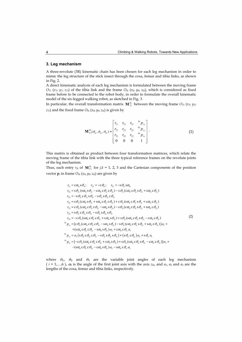
3. Leg mechanism

A three-revolute (3R) kinematic chain has been chosen for each leg mechanism in order to mimic the leg structure of the stick insect through the coxa, femur and tibia links, as shown in Fig. 2. A direct kinematic analysis of each leg mechanism is formulated between the moving frame OTi (xTi yTi zTi) of the tibia link and the frame O0i (x0i y0i z0i), which is considered as fixed frame before to be connected to the robot body, in order to formulate the overall kinematic model of the six-legged walking robot, as sketched in Fig. 3.

In particular, the overall transformation matrix 0iT iM between the moving frame OTi (xTi yTi

zTi) and the fixed frame O0i (x0i y0i z0i) is given by

0

11 12 13

0

0 21 22 23

1 2 3 0

31 32 33

( , , )

0 0 0 1

i

i x

i

i i y

T i i i i i

i z

r r r p

r r r p

r r r pϑ ϑ ϑ =M . (1)

This matrix is obtained as product between four transformation matrices, which relate the moving frame of the tibia link with the three typical reference frames on the revolute joints of the leg mechanism.

Thus, each entry rjk of 0iT iM for j,k = 1, 2, 3 and the Cartesian components of the position

vector pi in frame O0i (x0i y0i z0i) are given by

11 0 1 21 1 31 1 0

12 3 0 2 0 1 2 3 0 1 2 0 2

22 1 2 3 1 2 3

32 3 0 2 0 1 2 3 0 1 2 0 2

13 3 0 1 2 0

c s ; c ; s s

s (s s c c c ) c (c c s s c )

s c s s s c

s (c s s c c ) c (s c s c c )

c (c c c s

i i i

i i i i i i i i

i i i i i i

i i i i i i i i

i i i

r r r

r

r

r

r

α ϑ ϑ ϑ α

ϑ α ϑ α ϑ ϑ ϑ α ϑ ϑ α ϑ

ϑ ϑ ϑ ϑ ϑ ϑ

ϑ α ϑ α ϑ ϑ ϑ α ϑ ϑ α ϑ

ϑ α ϑ ϑ α

= = − = −

= − − +

= − −

= + + +

= − 2 3 0 1 2 0 2

23 1 2 3 1 2 3

33 3 0 1 2 0 2 3 0 1 2 0 2

0

3 0 1 2 0 2 3 0 1 2 0 2 3

0 1 2 0 2

s ) s (c c s s c )

s c c s s s

c (s c c c s ) s (s c s c c )

[c (c c c s s ) s (c c s s c )]

(c c c s s )

i i i i i

i i i i i i

i i i i i i i i

i

ix i i i i i i i i

i i i

r

r

p a

ϑ ϑ α ϑ ϑ α ϑ

ϑ ϑ ϑ ϑ ϑ ϑ

ϑ α ϑ ϑ α ϑ ϑ α ϑ ϑ α ϑ

ϑ α ϑ ϑ α ϑ ϑ α ϑ ϑ α ϑ

α ϑ ϑ α ϑ

− +

= −

= − + + −

= − − + +

+ −

( ) ( )

2 0 1 1

0

3 1 2 3 1 2 3 1 2 2 1 1

0

3 0 1 2 0 2 3 0 1 2 0 2 3

0 1 2 0 2 2 0 1 1

c c

s c c s s s s c s

[ c (s c c c s ) s (s c s c c )]

(s c c c s ) s c

i

i

iy i i i i i i i i i

i

iz i i i i i i i i

i i i i

a a

p a a a

p a

a a

α ϑ

ϑ ϑ ϑ ϑ ϑ ϑ ϑ ϑ ϑ

ϑ α ϑ ϑ α ϑ ϑ α ϑ ϑ α ϑ

α ϑ ϑ α ϑ α ϑ

+

= − + +

= − + + − +

− − −

(2)

where ϑ1i, ϑ2i and ϑ3i are the variable joint angles of each leg mechanism

( i = 1,…,6 ), α0 is the angle of the first joint axis with the axis z0i, and a1, a2 and a3 are the lengths of the coxa, femur and tibia links, respectively.

Mechanics and Simulation of Six-Legged Walking Robots 5

The inverse kinematic analysis of the leg mechanism is formulated through an algebraic approach. Thus, when the Cartesian components of the position vector pi are given in the

frame OFi (xFi yFi zFi), the variable joint angles ϑ 1i, ϑ 2i and ϑ 3i ( i = 1,…,6) can be expressed as

1 atan2 ( , )Fi Fi

i iy ixp pϑ = (3)

and

3 3 3atan2(s , c )i i iϑ ϑ ϑ= , (4)

where

2 2 2 2 2 2 2 2

1 1 2 3

3

2 3

2

3 3

( ) ( ) ( ) 2 ( ) ( )c

2

s 1 c

Fi Fi Fi Fi Fi

ix iy iz ix iy

i

i i

p p p a a p p a a

a aϑ

ϑ ϑ

+ + + − + − −=

= ± −

, (5)

x0iy0i ≡ yFi

z0i

h i

d i

L i

AEP0i

PEP0i

L/2

L/2

ySi

xSi

zSi

2iϑ

1iϑ

3iϑa1

a2

a3

α 0

robot body

pi

zTi

xTi

yTi

forward motion

zFi

Sipi

hT

tibia link

coxa link

femur link

swing phase

stance phase

Fig. 2. A 3R leg mechanism of the six-legged walking robot

Climbing & Walking Robots, Towards New Applications 6

and, in turn, by

2 2 2atan2(s , c )i i iϑ ϑ ϑ= , (6)

where

( ) ( )

( )

2 2

3 3 2 3 3

2 2 2

2 3 2 3 3

2 2 3 3

2

3 3

s ( ) ( ) cs

2 c

s cc

s

Fi Fi Fi

i ix iy iz i

i

i

Fi

iz i i

i

i

a p p p a a

a a a a

p a a

a

ϑ ϑϑ

ϑ

ϑ ϑϑ

ϑ

+ + += −

+ +

+ += −

. (7)

Therefore, the Eqs. (1-7) let to formulate the overall kinematic model of the six-legged walking robot, as proposed in the following.

4. Kinematic model of the six-legged walking robot

Referring to Figs. 2 and 3, the kinematic model of a six-legged walking robot is formulated through a direct kinematic analysis between the moving frame OTi (xTi yTi zTi) of the tibia link and the inertia frame O (X Y Z).

In general, a six-legged walking robot has 24 d.o.f.s, where 18 d.o.f.s are given by ϑ 1i, ϑ 2i

and ϑ 3i (i = 1,…,6) for the six 3R leg mechanisms and 6 d.o.f.s are given by the robot body, which are reduced in this case at only 1 d.o.f. that is given by XG in order to consider the pure translation of the robot body along the X-axis.Thus, the equation of motion XG (t) of the robot body is assigned as input of the proposed

algorithm, while ϑ 1i (t), ϑ 2i (t) and ϑ 3i (t) for i = 1,…,6 are expressed through an inverse kinematic analysis of the six 3R leg mechanisms when the equation of motion of each leg tip is given and the trajectory shape of each leg tip during the swing phase is assigned. In particular, the transformation matrix MG of the frame G (xG yG zG) on the robot body with respect to the inertia frame O (X Y Z ) is expressed as

( )

1 0 0

0 1 0

0 0 1

0 0 0 1

GX

GY

G G

GZ

X

p

p

p=M , (8)

where pGX = XG, pGY = 0 and pGZ = hG.

The transformation matrix G

BiM of the frame OBi (xBi yBi zBi) on the robot body with respect to

the frame G (xG yG zG) is expressed by

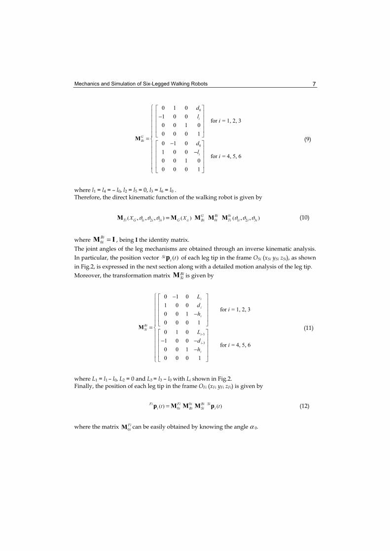
Mechanics and Simulation of Six-Legged Walking Robots 7

0

0

0 1 0

1 0 0 for = 1, 2, 3

0 0 1 0

0 0 0 1

0 1 0

1 0 0for = 4, 5, 6

0 0 1 0

0 0 0 1

i

G

Bi

i

d

li

d

li

−

=−

−

M (9)

where l1 = l4 = – l0, l2 = l5 = 0, l3 = l6 = l0 . Therefore, the direct kinematic function of the walking robot is given by

1 2 3 1 2 3( ) ( ) ( ), , , , ,G

G Bi 0i

Ti G i i i G Bi 0i Ti i i iX Xϑ ϑ ϑ ϑ ϑ ϑ=M M M M M (10)

whereBi

0i =M I , being I the identity matrix.

The joint angles of the leg mechanisms are obtained through an inverse kinematic analysis.

In particular, the position vector ( )Sii tp of each leg tip in the frame OSi (xSi ySi zSi), as shown

in Fig.2, is expressed in the next section along with a detailed motion analysis of the leg tip.

Moreover, the transformation matrix BiSiM is given by

3

3

0 1 0

1 0 0 for = 1, 2, 3

0 0 1

0 0 0 1

0 1 0

1 0 0for = 4, 5, 6

0 0 1

0 0 0 1

i

i

i

Bi

Si

i-

i-

i

L

di

h

L

di

h

−

−

=

− −

−

M (11)

where L1 = l1 – l0, L2 = 0 and L3 = l3 – l0 with Li shown in Fig.2. Finally, the position of each leg tip in the frame OFi (xFi yFi zFi) is given by

0

0( ) ( )Fi Fi i Bi Si

i i Bi Si it t=p M M M p (12)

where the matrix 0

Fi

iM can be easily obtained by knowing the angle α 0.

Climbing & Walking Robots, Towards New Applications 8

Therefore, substituting the Cartesian components of ( )Fii tp in Eqs. (3), (5) and (7), the joint

angles ϑ 1i, ϑ 2i and ϑ 3i (i = 1,…,6) can be obtained.

xB3 yB3

zB3

xB2

yB2

zB2x01

y 01

z01

yG

xG

zG

G

PEP1

AEP2

PEP2 AEP3

PEP3

forward motion

x03

z03

y 03

x 02

y 02

z02

zB1

yB1

xB1

y S3

zS3xS3

yS2

zS2x S2

yS1

x S1

Y

X

Z

O

robot body

pG

zS1AEP1

hG

G

Fig. 3. Kinematic scheme of the six-legged walking robot

5. Motion analysis of the leg tip

The gait of the robot is obtained by a suitable coordination of each leg tip, which is fundamental to ensure the static stability of the robot during the walking. Thus, a typical motion of each leg tip has to be imposed through the position vector Sipi(t), even if a variable gait of the robot can be obtained according to the imposed speed of the robot body. Referring to Figs. 2 to 4, the position vector Sipi(t) of each leg tip can be expressed as

( ) 1T

Si Si Si Si

i ix iy izt p p p=p (13)

in the local frame OSi (xSi ySi zSi) for i = 1,…,6, which is considered as attached and moving with the robot body. Referring to Fig. 4, the x-coordinate Sipix of vector Sipi(t) is given by the following system of difference equations

( ) ( )( )

( ) ( )

for 1

for 0

ix r iSi

ix

ix p i

t V tt t

t V t

p t sp

p t s

−+ ∆

+

∆ ==

∆ = (14)

where Vr is the velocity of the tip of each leg mechanism during the retraction motion of the stance phase, even defined power stroke, since producing the motion of the robot body, and Vp is the velocity along the robot body of the tip of each leg mechanism during the protraction motion of the swing phase, even defined return stroke, since producing the forward motion of the leg mechanism.

Mechanics and Simulation of Six-Legged Walking Robots 9

hT

zSi

xSi OSi

Vp

Vp

Vr < Vp

VSi

pi

L/2 L/2

AEP0 PEP0

VG = Vrswing phase

stance phase

(t0 )i

(tf )i

Fig. 4. Trajectory and velocities of the tip of each leg mechanism during the stance and swing phases

Parameter si defines the state of the i-th leg, which is equal to 1 for the retraction state, or stance phase, and equal to 0 for the protraction state, or swing phase. Both velocities Vp and Vr are supposed to be constant and identical for all legs, for which the speed VG of the center of mass of the robot body is equal to Vr because of the relative motion. In fact, during the stance phase (power stroke), each tip leg moves back with velocity Vr with respect to the robot body and, consequentially, this moves ahead with the

same velocity. Thus, the function ( )Si

ixp t of Eq. (2) for i = 1, …, 6 is linear periodic function.

Moreover, it is quite clear that the static stability of the six-legged walking robot is obtained only when Vr (=VG) < Vp, because the robot body cannot move forward faster than its legs move in the same direction during the swing phase. Likewise, Sipiy is equal to zero in order to obtain a vertical planar trajectory, while Sipiz is given by

0

0

( )

( )( )

0 for 1

sin for 0

i

Si iiz

T ii i

f

t

tt

s

p t th s

t tπ

=

= −=

−

(15)

where hT is the amplitude of the sinusoid and time t is the general instant, while 0it and

ift

are the starting and ending times of the swing phase, respectively.

Times 0it and

ift take into account the mechanism of the leg coordination, which give a

suitable variation of AEPi and PEPi in order to ensure the static stability. Thus, referring to the time diagrams of VG in Fig. 5, the time diagrams of Figs. 6 to 8 have been obtained. In particular, Fig. 5 shows the time diagrams of the robot speeds VG = 0.05, 0.1, 0.5 and 0.9 mm/s for the case of constant acceleration a = 0.002 mm/s2. Thus, the transient periods t = 25, 50, 250 and 450 s for the speeds VG = 0.05, 0.1, 0.5 and 0.9 mm/s of the robot body are obtained respectively before to reach the steady-state condition at

Climbing & Walking Robots, Towards New Applications 10

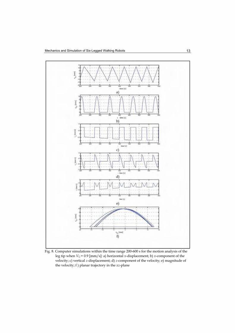
constant speed. The time diagrams of Figs. 6 to 8 show the horizontal x-displacement, the x-component of the velocity, the vertical z-displacement, the z-component of the velocity, the magnitude of the velocity and the trajectory of the leg tip 1 (front left leg) of the six-legged walking robot. Thus, before to analyze in depth the time diagrams of Figs. 6 to 8, it may be useful to refer to the motion analysis of the leg tip and to remind that the protraction speed Vp along the axis of the robot body has been assigned as constant and equal to 1 mm/s for the swing phase of the leg tip. In other words, only the retraction speed Vr can be changed since related and equal to the robot speed VG, which is assigned as input data. Consequently, the range time during the stance phase between two consecutive steps of each leg can vary in significant way because of the different imposed speeds Vr = VG, while the time range to perform the swing phase of each leg is almost the same because of the same speed Vp and similar overall x-displacements. In particular, Fig. 6 show computer simulations between the time range 200 - 340 s, which is after the transient periods of 25 and 50 s for VG = 0.05 and 0.1 mm/s, respectively. Thus, both x-component of the velocity, protraction speed Vp = 1 mm/s and retraction speed Vr = VG = 0.05 and 0.1 mm/s, are constant versus time. Instead, Figs. 7 and 8 show two computer simulations between the time ranges of 0 - 400 s and 200 - 600 s, which are greater than the transient periods of 250 and 450 s for the robot speeds VG of 0.5 and 0.9 mm/s, respectively. Thus, the transient behavior of the velocities is also shown at the constant acceleration of 0.002 mm/s2. In fact, during these time ranges of 250 and 450 s, the protraction speed Vp is always constant and equal to 1 mm/s, while the retraction speed Vr

varies linearly according to the constant acceleration, before to reach the steady-state condition and to equalize the speed VG of the robot body. The same effect is also shown by the time diagrams of Figs. 7e and 8e, which show the magnitude of the velocity. Moreover, single loop trajectories are shown in the simulations of Figs. 6e and 6m, because one step only is performed by the leg mechanism 1, while multi-loop trajectories are shown in the simulations of Figs. 7f and 8f, because 3 (three) and 7 (seven) steps are performed by the leg mechanism 1, respectively. The variation of the step length is also evident in Figs. 7f and 8f because of the influence mechanisms for the leg coordination.

Fig. 5. Time diagrams of the robot body speed for a constant acceleration a = 0.002 mm/s2

and VG = 0.05, 0.1, 0.5 and 0.9 mm/s

Mechanics and Simulation of Six-Legged Walking Robots 11

Fig. 6. Computer simulations for the motion analysis of the leg tip of a six-legged walking

robot when VG = 0.05 and 0.1 [mm/s]: a) and g) horizontal x-displacement; b) and h)

vertical z-displacement; c) and i) x-component of the velocity; d) and l) z-component

of the velocity; e) and m) planar trajectory in the xz-plane; f) and n) magnitude of the

velocity

Climbing & Walking Robots, Towards New Applications 12

Fig. 7. Computer simulations within the time range 0 - 400 s for the motion analysis of the leg tip when VG = 0.5 [mm/s]: a) horizontal x-displacement; b) x-component of the velocity; c) vertical z-displacement; d) z-component of the velocity; e) magnitude of the velocity; f ) planar trajectory in the xz-plane

Mechanics and Simulation of Six-Legged Walking Robots 13

Fig. 8. Computer simulations within the time range 200-600 s for the motion analysis of the

leg tip when VG = 0.9 [mm/s]: a) horizontal x-displacement; b) x-component of the

velocity; c) vertical z-displacement; d) z-component of the velocity; e) magnitude of

the velocity; f ) planar trajectory in the xz-plane

Climbing & Walking Robots, Towards New Applications 14

6. Gait analysis

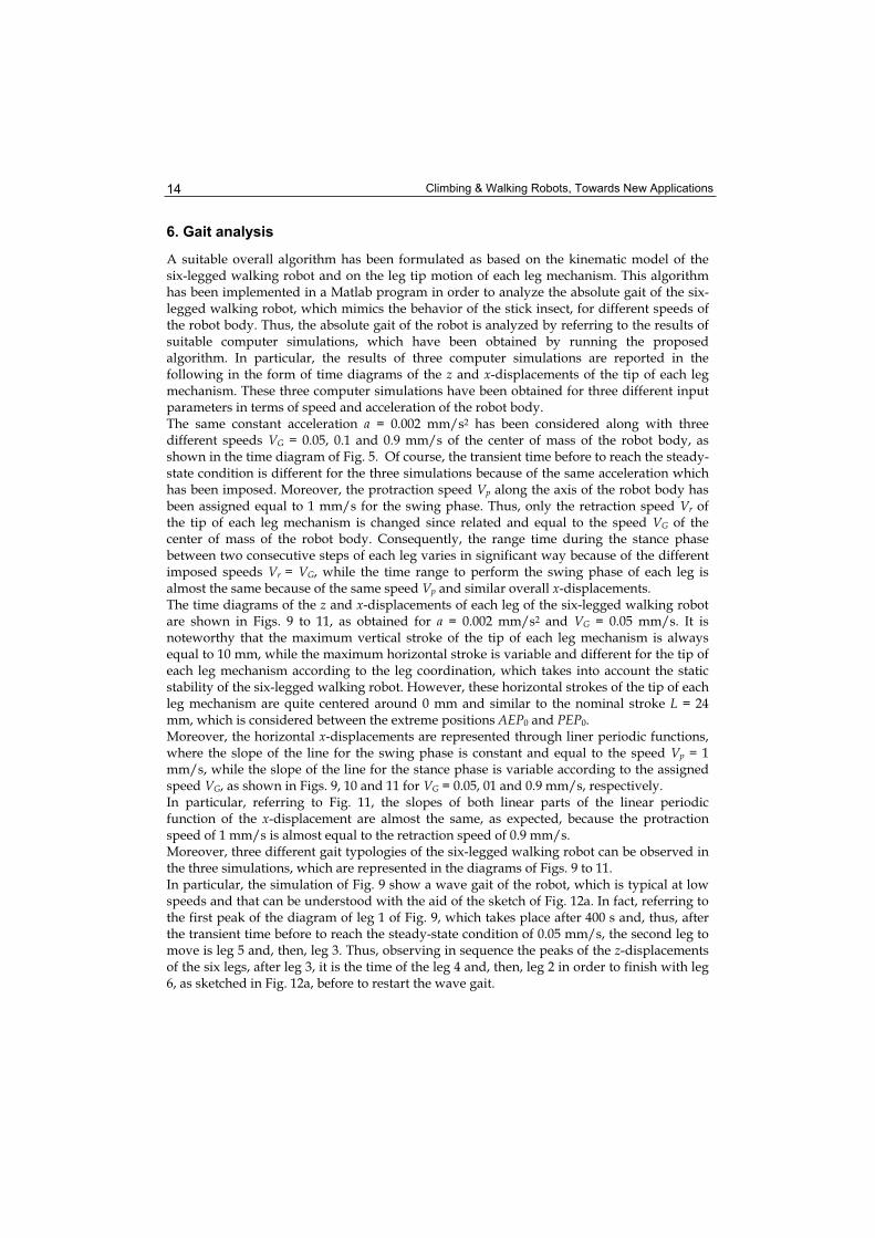
A suitable overall algorithm has been formulated as based on the kinematic model of the six-legged walking robot and on the leg tip motion of each leg mechanism. This algorithm has been implemented in a Matlab program in order to analyze the absolute gait of the six-legged walking robot, which mimics the behavior of the stick insect, for different speeds of the robot body. Thus, the absolute gait of the robot is analyzed by referring to the results of suitable computer simulations, which have been obtained by running the proposed algorithm. In particular, the results of three computer simulations are reported in the following in the form of time diagrams of the z and x-displacements of the tip of each leg mechanism. These three computer simulations have been obtained for three different input parameters in terms of speed and acceleration of the robot body. The same constant acceleration a = 0.002 mm/s2 has been considered along with three different speeds VG = 0.05, 0.1 and 0.9 mm/s of the center of mass of the robot body, as shown in the time diagram of Fig. 5. Of course, the transient time before to reach the steady-state condition is different for the three simulations because of the same acceleration which has been imposed. Moreover, the protraction speed Vp along the axis of the robot body has been assigned equal to 1 mm/s for the swing phase. Thus, only the retraction speed Vr of the tip of each leg mechanism is changed since related and equal to the speed VG of the center of mass of the robot body. Consequently, the range time during the stance phase between two consecutive steps of each leg varies in significant way because of the different imposed speeds Vr = VG, while the time range to perform the swing phase of each leg is almost the same because of the same speed Vp and similar overall x-displacements. The time diagrams of the z and x-displacements of each leg of the six-legged walking robot are shown in Figs. 9 to 11, as obtained for a = 0.002 mm/s2 and VG = 0.05 mm/s. It is noteworthy that the maximum vertical stroke of the tip of each leg mechanism is always equal to 10 mm, while the maximum horizontal stroke is variable and different for the tip of each leg mechanism according to the leg coordination, which takes into account the static stability of the six-legged walking robot. However, these horizontal strokes of the tip of each leg mechanism are quite centered around 0 mm and similar to the nominal stroke L = 24 mm, which is considered between the extreme positions AEP0 and PEP0.Moreover, the horizontal x-displacements are represented through liner periodic functions, where the slope of the line for the swing phase is constant and equal to the speed Vp = 1 mm/s, while the slope of the line for the stance phase is variable according to the assigned speed VG, as shown in Figs. 9, 10 and 11 for VG = 0.05, 01 and 0.9 mm/s, respectively. In particular, referring to Fig. 11, the slopes of both linear parts of the linear periodic function of the x-displacement are almost the same, as expected, because the protraction speed of 1 mm/s is almost equal to the retraction speed of 0.9 mm/s. Moreover, three different gait typologies of the six-legged walking robot can be observed in the three simulations, which are represented in the diagrams of Figs. 9 to 11. In particular, the simulation of Fig. 9 show a wave gait of the robot, which is typical at low speeds and that can be understood with the aid of the sketch of Fig. 12a. In fact, referring to the first peak of the diagram of leg 1 of Fig. 9, which takes place after 400 s and, thus, after the transient time before to reach the steady-state condition of 0.05 mm/s, the second leg to move is leg 5 and, then, leg 3. Thus, observing in sequence the peaks of the z-displacements of the six legs, after leg 3, it is the time of the leg 4 and, then, leg 2 in order to finish with leg 6, as sketched in Fig. 12a, before to restart the wave gait.

Mechanics and Simulation of Six-Legged Walking Robots 15

0 200 400 600 800 1000 1200 1400 1600 1800

0

5

10

time [s] (Leg 1)

z S1

0 200 400 600 800 1000 1200 1400 1600 1800

0

5

10

time [s] (Leg 2)

z S2

0 200 400 600 800 1000 1200 1400 1600 1800

0

5

10

time [s] (Leg 3)

z S3

0 200 400 600 800 1000 1200 1400 1600 1800

0

5

10

time [s] (Leg 4)

z S4

0 200 400 600 800 1000 1200 1400 1600 1800

0

5

10

time [s] (Leg 5)

z S5

0 200 400 600 800 1000 1200 1400 1600 1800

0

5

10

time [s] (Leg 6)

z S6

a)

0 200 400 600 800 1000 1200 1400 1600 1800-20

0

20

time [s] (Leg 1)

xS

1

0 200 400 600 800 1000 1200 1400 1600 1800-20

0

20

time [s] (Leg 2)

xS

2

0 200 400 600 800 1000 1200 1400 1600 1800-20

0

20

time [s] (Leg 3)

xS

3

0 200 400 600 800 1000 1200 1400 1600 1800-20

0

20

time [s] (Leg 4)

xS

4

0 200 400 600 800 1000 1200 1400 1600 1800-20

0

20

time [s] (Leg 5)

xS

5

0 200 400 600 800 1000 1200 1400 1600 1800-20

0

20

time [s] (Leg 6)

xS

6

b)

Fig. 9. Displacements of the leg tip for VG = 0.05 mm/s and a = 0.002 mm/s2: a) vertical z-displacement; b) horizontal x-displacement

Climbing & Walking Robots, Towards New Applications 16

0 200 400 600 800 1000 1200 1400 1600 1800

0

5

10

time [s] (Leg 1)

z S1

0 200 400 600 800 1000 1200 1400 1600 1800

0

5

10

time [s] (Leg 2)

z S2

0 200 400 600 800 1000 1200 1400 1600 1800

0

5

10

time [s] (Leg 3)

z S3

0 200 400 600 800 1000 1200 1400 1600 1800

0

5

10

time [s] (Leg 4)

z S4

0 200 400 600 800 1000 1200 1400 1600 1800

0

5

10

time [s] (Leg 5)

z S5

0 200 400 600 800 1000 1200 1400 1600 1800

0

5

10

time [s] (Leg 6)

z S6

a)

0 200 400 600 800 1000 1200 1400 1600 1800-20

0

20

time [s] (Leg 1)

xS

1

0 200 400 600 800 1000 1200 1400 1600 1800-20

0

20

time [s] (Leg 2)

xS

2

0 200 400 600 800 1000 1200 1400 1600 1800-20

0

20

time [s] (Leg 3)

xS

3

0 200 400 600 800 1000 1200 1400 1600 1800-20

0

20

time [s] (Leg 4)

xS

4

0 200 400 600 800 1000 1200 1400 1600 1800-20

0

20

time [s] (Leg 5)

xS

5

0 200 400 600 800 1000 1200 1400 1600 1800-20

0

20

time [s] (Leg 6)

xS

6

b)

Fig. 10. Displacements of the leg tip for VG = 0.1 mm/s and a = 0.002 mm/s2: a) vertical z-displacement; b) horizontal x-displacement

Mechanics and Simulation of Six-Legged Walking Robots 17

0 200 400 600 800 1000 1200 1400 1600 1800

0

5

10

time [s] (Leg 1)

z S1

0 200 400 600 800 1000 1200 1400 1600 1800

0

5

10

time [s] (Leg 2)

z S2

0 200 400 600 800 1000 1200 1400 1600 1800

0

5

10

time [s] (Leg 3)

z S3

0 200 400 600 800 1000 1200 1400 1600 1800

0

5

10

time [s] (Leg 4)

z S4

0 200 400 600 800 1000 1200 1400 1600 1800

0

5

10

time [s] (Leg 5)

z S5

0 200 400 600 800 1000 1200 1400 1600 1800

0

5

10

time [s] (Leg 6)

z S6

a)

0 200 400 600 800 1000 1200 1400 1600 1800-20

0

20

time [s] (Leg 1)

xS

1

0 200 400 600 800 1000 1200 1400 1600 1800-20

0

20

time [s] (Leg 2)

xS

2

0 200 400 600 800 1000 1200 1400 1600 1800-20

0

20

time [s] (Leg 3)

xS

3

0 200 400 600 800 1000 1200 1400 1600 1800-20

0

20

time [s] (Leg 4)

xS

4

0 200 400 600 800 1000 1200 1400 1600 1800-20

0

20

time [s] (Leg 5)

xS

5

0 200 400 600 800 1000 1200 1400 1600 1800-20

0

20

time [s] (Leg 6)

xS

6

b)

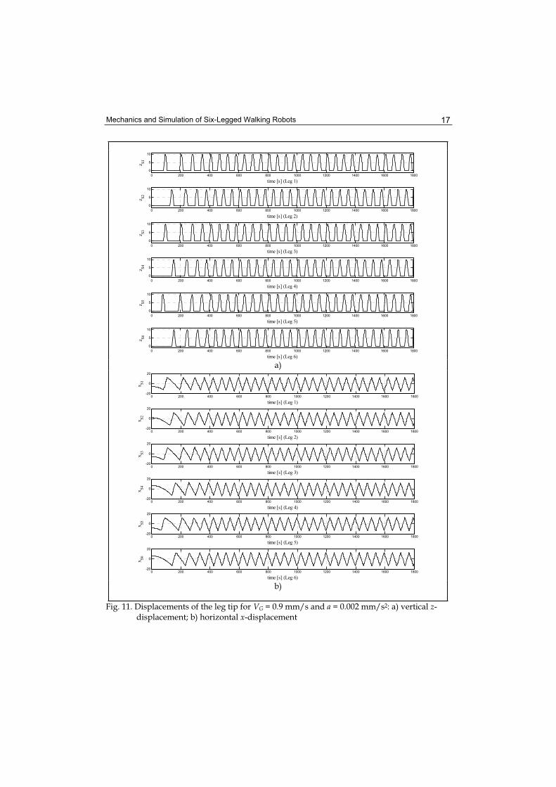
Fig. 11. Displacements of the leg tip for VG = 0.9 mm/s and a = 0.002 mm/s2: a) vertical z-displacement; b) horizontal x-displacement

Climbing & Walking Robots, Towards New Applications 18

1 2 3

4 5 6

1 2 3

4 5 6

1 2 3

4 5 6

a) b) c)

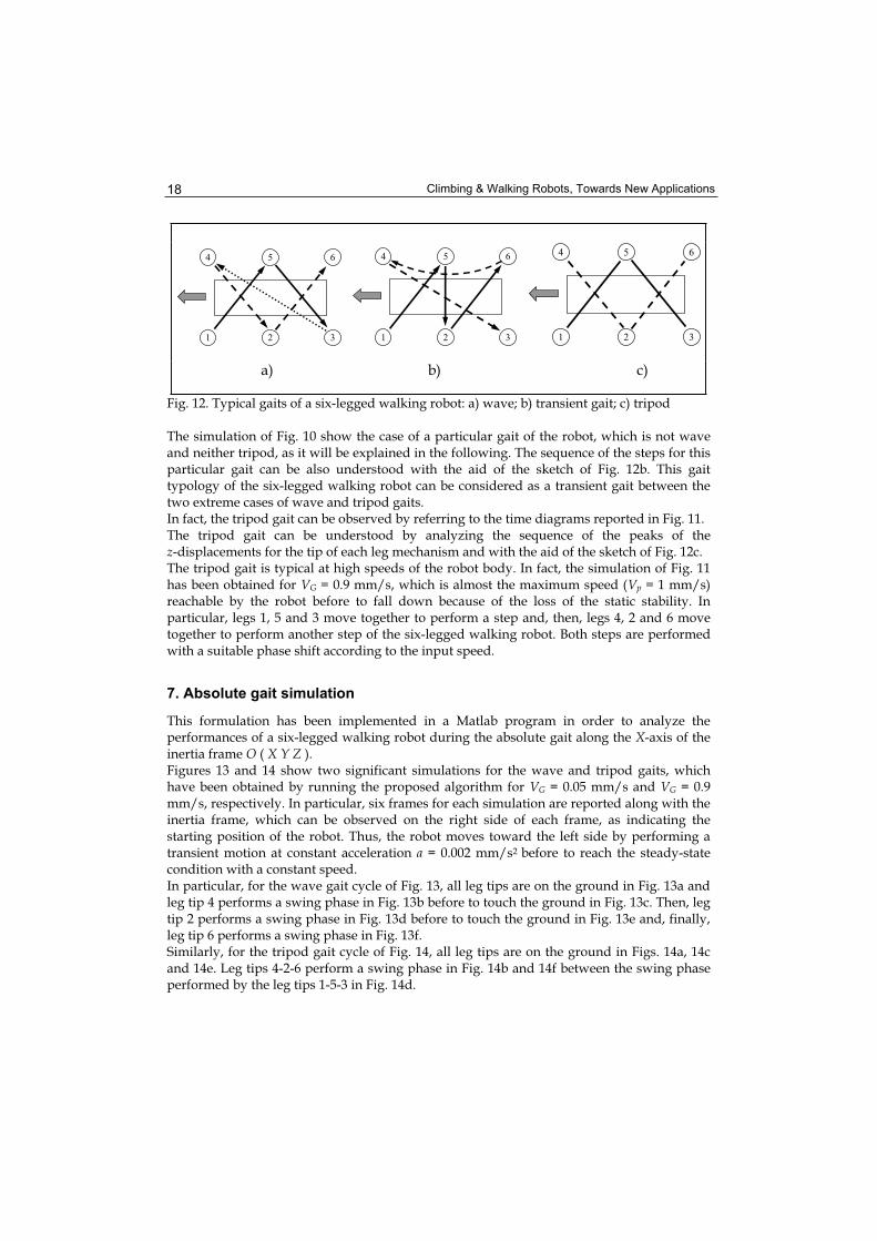
Fig. 12. Typical gaits of a six-legged walking robot: a) wave; b) transient gait; c) tripod

The simulation of Fig. 10 show the case of a particular gait of the robot, which is not wave and neither tripod, as it will be explained in the following. The sequence of the steps for this particular gait can be also understood with the aid of the sketch of Fig. 12b. This gait typology of the six-legged walking robot can be considered as a transient gait between the two extreme cases of wave and tripod gaits. In fact, the tripod gait can be observed by referring to the time diagrams reported in Fig. 11. The tripod gait can be understood by analyzing the sequence of the peaks of the z-displacements for the tip of each leg mechanism and with the aid of the sketch of Fig. 12c. The tripod gait is typical at high speeds of the robot body. In fact, the simulation of Fig. 11 has been obtained for VG = 0.9 mm/s, which is almost the maximum speed (Vp = 1 mm/s) reachable by the robot before to fall down because of the loss of the static stability. In particular, legs 1, 5 and 3 move together to perform a step and, then, legs 4, 2 and 6 move together to perform another step of the six-legged walking robot. Both steps are performed with a suitable phase shift according to the input speed.

7. Absolute gait simulation

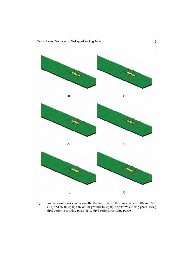
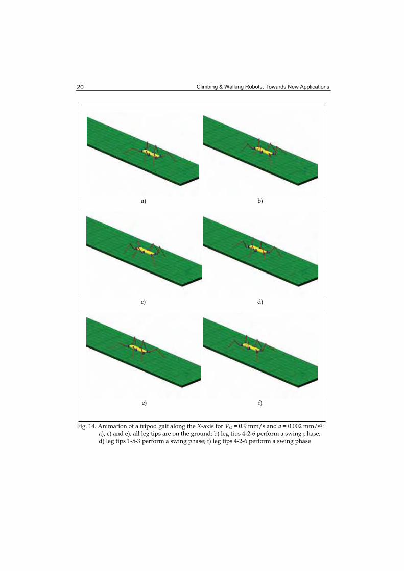
This formulation has been implemented in a Matlab program in order to analyze the performances of a six-legged walking robot during the absolute gait along the X-axis of the inertia frame O ( X Y Z ). Figures 13 and 14 show two significant simulations for the wave and tripod gaits, which have been obtained by running the proposed algorithm for VG = 0.05 mm/s and VG = 0.9 mm/s, respectively. In particular, six frames for each simulation are reported along with the inertia frame, which can be observed on the right side of each frame, as indicating the starting position of the robot. Thus, the robot moves toward the left side by performing a transient motion at constant acceleration a = 0.002 mm/s2 before to reach the steady-state condition with a constant speed. In particular, for the wave gait cycle of Fig. 13, all leg tips are on the ground in Fig. 13a and leg tip 4 performs a swing phase in Fig. 13b before to touch the ground in Fig. 13c. Then, leg tip 2 performs a swing phase in Fig. 13d before to touch the ground in Fig. 13e and, finally, leg tip 6 performs a swing phase in Fig. 13f. Similarly, for the tripod gait cycle of Fig. 14, all leg tips are on the ground in Figs. 14a, 14c and 14e. Leg tips 4-2-6 perform a swing phase in Fig. 14b and 14f between the swing phase performed by the leg tips 1-5-3 in Fig. 14d.

Mechanics and Simulation of Six-Legged Walking Robots 19

a) b)

c) d)

e) f)

Fig. 13. Animation of a wave gait along the X-axis for VG = 0.05 mm/s and a = 0.002 mm/s2:a), c) and e), all leg tips are on the ground; b) leg tip 4 performs a swing phase; d) leg tip 2 performs a swing phase; f) leg tip 6 performs a swing phase

Climbing & Walking Robots, Towards New Applications 20

a) b)

c) d)

e) f)

Fig. 14. Animation of a tripod gait along the X-axis for VG = 0.9 mm/s and a = 0.002 mm/s2:a), c) and e), all leg tips are on the ground; b) leg tips 4-2-6 perform a swing phase; d) leg tips 1-5-3 perform a swing phase; f) leg tips 4-2-6 perform a swing phase

Mechanics and Simulation of Six-Legged Walking Robots 21

8. Conclusions

The mechanics and locomotion of six-legged walking robots has been analyzed by considering a simple “technical design”, in which the biological inspiration is only given by the trivial observation that some insects use six legs to obtain a static walking, and considering a “biological design”, in which we try to emulate, in every detail, the locomotion of a particular specie of insect, as the “cockroach” or “stick” insects. In particular, as example of the mathematical approach to analyze the mechanics and locomotion of six-legged walking robots, the kinematic model of a six-legged walking robot, which mimics the biological structure and locomotion of the stick insect, has been formulated according to the Cruse-based leg control system. Thus, the direct kinematic analysis between the moving frame of the tibia link and the inertia frame that is fixed to the ground has been formulated for the six 3R leg mechanisms, where the joint angles have been expressed through an inverse kinematic analysis when the trajectory of each leg tip is given. This aspect has been considered in detail by analyzing the motion of each leg tip of the six-legged walking robot in the local frame, which is considered as attached and moving with the robot body. Several computer simulations have been reported in the form of time diagrams of the horizontal and vertical displacements along with the horizontal and vertical components of the velocities for a chosen leg of the robot. Moreover, single and multi-loop trajectories of a leg tip have been shown for different speeds of the robot body, in order to put in evidence the effects of the Cruse-based leg control system, which ensures the static stability of the robot at different speeds by adjusting the step length of each leg during the walking. Finally, the gait analysis and simulation of the six-legged walking robot, which mimics the locomotion of the stick insect , have been carried out by referring to suitable time diagrams of the z and x-displacements of the six legs, which have shown the extreme typologies of the wave and tripod gaits at low and high speeds of the robot body, respectively.

9. References

Song, S.M. & Waldron, K.J., (1989). Machines That Walk: the Adaptive Suspension Vehicle, MIT Press, ISBN 0-262-19274-8, Cambridge, Massachusetts.

Raibert, M.H., (1986). Legged Robots That Balance, MIT Press, ISBN 0-262-18117-7, Cambridge, Massachusetts.

Delcomyn, F. & Nelson, M. E. (2000). Architectures for a biomimetic hexapod robot, Roboticsand Autonomous Systems, Vol. 30, pp.5–15.

Quinn, R. D., Nelson, G. M., Bachmann, R. J., Kingsley, D. A., Offi J. & Ritzmann R. E., (2001). Insect Designs for Improved Robot Mobility, Proceedings of the 4th

International Conference on Climbing and Walking Robots, Berns and Dillmann (Eds), Professional Engineering Publisher, London, pp. 69-76.

Espenschied, K.S., Quinn, R.D., Beer, R.D. & Chiel H.J., (1996). Biologically based distributed control and local reflexes improve rough terrain locomotion in a hexapod robot, Robotics and Autonomous Systems, Vol. 18, pp. 59-64.

Cruse, H., (1990). What mechanisms coordinate leg movement in walking arthropods ?, Trends in Neurosciences, Vol. 13, pp. 15-21.

Cruse, H. & Bartling, Ch., (1995). Movement of joint angles in the legs of a walking insect, Carausius morosus, J. Insect Physiology, Vol. 41 (9), pp.761-771.

Climbing & Walking Robots, Towards New Applications 22

Frantsevich, F. & Cruse, H., (1997). The stick insect, Obrimus asperrimus (Phasmida, Bacillidae) walking on different surfaces, J. of Insect Physiology, Vol. 43 (5), pp.447-455.

Cruse, H., Kindermann, T., Schumm, M., Dean, J. and Schmitz, J., (1998). Walknet - a biologically inspired network to control six-legged walking, Neural Networks,Vol.11, pp. 1435-1447.

Cymbalyuk, G.S., Borisyuk, R.M., Müeller-Wilm, U. & Cruse, H., (1998). Oscillatory network controlling six-legged locomotion. Optimization of model parameters, NeuralNetworks, Vol. 11, pp. 1449-1460.

Cruse, H., (2002). The functional sense of central oscillations in walking, Biological Cybernetics, Vol. 86, pp. 271-280.

Volker, D., Schmitz, J. & Cruse, H., (2004). Behaviour-based modelling of hexapod locomotion: linking biology and technical application, Arthropod Structure & Development, Vol. 33, pp. 237–250.

Dean, J., (1991). A model of leg coordination in the stick insect, Carausius morosus. I. Geometrical consideration of coordination mechanisms between adjacent legs. Biological Cybernetics, Vol. 64, pp. 393-402.

Dean, J., (1991). A model of leg coordination in the stick insect, Carausius morosus. II. Description of the kinematic model and simulation of normal step patterns. Biological Cybernetics, Vol. 64, pp. 403-411.

Dean, J., (1992). A model of leg coordination in the stick insect, Carausius morosus, III. Responses to perturbations of normal coordination, Biological Cybernetics, Vol. 66, pp. 335-343.

Dean, J., (1992). A model of leg coordination in the stick insect, Carausius morosus, IV. Comparison of different forms of coordinating mechanisms, Biological Cybernetics,Vol. 66, pp. 345-355.

Mueller-Wilm, U., Dean, J., Cruse, H., Weidermann, H.J., Eltze, J. & Pfeiffer, F., (1992). Kinematic model of a stick insect as an example of a six-legged walking system, Adaptive Behavior, Vol. 1 (2), pp. 155–169.

Figliolini, G. & Ripa, V., (2005). Kinematic Model and Absolute Gait Simulation of a Six-Legged Walking Robot, In: Climbing and Walking Robots, Manuel A. Armada & Pablo González de Santos (Ed), pp. 889-896, Springer, ISBN 3-540-22992-6, Berlin.

Figliolini, G., Rea, P. & Ripa, V., (2006). Analysis of the Wave and Tripod Gaits of a Six-Legged Walking Robot, Proceedings of the 9th International Conference on Climbing and Walking Robots and Support Technologies for Mobile Machines, pp. 115-122, Brussels, Belgium, September 2006.

Figliolini, G., Rea, P. & Stan, S.D., (2006). Gait Analysis of a Six-Legged Walking Robot When a Leg Failure Occurs, Proceedings of the 9th International Conference on Climbing and Walking Robots and Support Technologies for Mobile Machines, pp. 276-283, Brussels, Belgium, September 2006.

Figliolini, G., Stan, S.D. & Rea, P. (2007). Motion Analysis of the Leg Tip of a Six-Legged Walking Robot, Proceedings of the 12th IFToMM World Congress, Besançon (France), paper number 912.

Climbing and Walking Robots: towards New ApplicationsEdited by Houxiang Zhang

ISBN 978-3-902613-16-5Hard cover, 546 pagesPublisher I-Tech Education and PublishingPublished online 01, October, 2007Published in print edition October, 2007

InTech EuropeUniversity Campus STeP Ri Slavka Krautzeka 83/A 51000 Rijeka, Croatia Phone: +385 (51) 770 447 Fax: +385 (51) 686 166www.intechopen.com

InTech ChinaUnit 405, Office Block, Hotel Equatorial Shanghai No.65, Yan An Road (West), Shanghai, 200040, China

Phone: +86-21-62489820 Fax: +86-21-62489821

With the advancement of technology, new exciting approaches enable us to render mobile robotic systemsmore versatile, robust and cost-efficient. Some researchers combine climbing and walking techniques with amodular approach, a reconfigurable approach, or a swarm approach to realize novel prototypes as flexiblemobile robotic platforms featuring all necessary locomotion capabilities. The purpose of this book is to providean overview of the latest wide-range achievements in climbing and walking robotic technology to researchers,scientists, and engineers throughout the world. Different aspects including control simulation, locomotionrealization, methodology, and system integration are presented from the scientific and from the technical pointof view. This book consists of two main parts, one dealing with walking robots, the second with climbing robots.The content is also grouped by theoretical research and applicative realization. Every chapter offers aconsiderable amount of interesting and useful information.

How to referenceIn order to correctly reference this scholarly work, feel free to copy and paste the following:

Giorgio Figliolini and Pierluigi Rea (2007). Mechanics and Simulation of Six-Legged Walking Robots, Climbingand Walking Robots: towards New Applications, Houxiang Zhang (Ed.), ISBN: 978-3-902613-16-5, InTech,Available from:http://www.intechopen.com/books/climbing_and_walking_robots_towards_new_applications/mechanics_and_simulation_of_six-legged_walking_robots