MEFA II UNIT COMPLETE NOTES

PRODUCTION ANALYSISProduction in Economics means creation of goods and services which have exchange value. In other words, it implies creation of utilities. Process of production creates utility by conferring form utility, place utility and time utility. Production is an organized activity of transforming input into outputs to satisfy the demand for the commodities and services of the company.

Inputs refers to the all those things which a firm buts and employs to produce a particular product. Output means the quantity of goods in the finished form produced by the firm for selling. Production analysis deals with physical production and supply side of the market.

Definition for Production:According to the Parkinson:“Production is the organized activity of transformation resources into finished products in the form of goods and services”.

According to the J.R. Hicks:“Production is any acidity directed to the satisfaction of other people’s want through exchange”

Production Function: Production function expresses a functional or technical relationship between physical inputs and physical outputs of a firm at any particular time period. The output is thus a function of inputs. Production is the result of combination of factors of production land, labor, capital and organization. The factors used for production are called “inputs”. The production we get is called “output”. The production functions show the maximum rates of output that can be obtained from different combinations of inputs in a given time with a given state of technology, managerial ability etc.

Production function enables production manager to understand how better he can make use of technology to its greatest potential

Durga Chaitanya Prasad Navulla M.Com, MBA SITE. 1

Definition for Production function:

“The production function is the name given to the relationship between the rates of productive services and the rates of output of the product.” -------Stigler

“Production function is that function which defines the maximum amount of output that can be produced with a given set of inputs”. -------Michael R Baye.

Production Function:It can be expressed in an allegorical equation:Q= f (M 1 , M 2 , M 3 ,M 4M 5 , I . .. .. . .n )Where Q stands for the quantity of outputM1= MaterialsM2= MenM3= MachinesM4= MoneyM5= ManagementI= Information

Each form has its own production function depending on the technical knowledge and managerial ability. An improvement in the technical knowledge or managerial ability will bring about a new production function. Here output is the function of inputs, the output becomes the dependent variable and inputs are the independent variables. Production function has to be expressed in a precise mathematical equation i.e.

Y=a+bxIt is showing the there is constant relationship between application of input (x) and the amount of output(Y). The production function may be fixed production function are variable production function. In fixed production function each level of output requires a unique combination of inputs. On the other hand a variable production proportion production function is one which the same level of output may be produced by two or more combinations of inputs.

Assumptions:The production function is related to a particular period of timeThe level of technology remains constantThe producer is using the best and most technique availableThe factors of production are divisibleProduction can be fitted to a short run or to long run.Utilization of inputs at maximum level of efficiency.

Importance of production function:When inputs are specified in physical units, production function helps to estimate the level of productionWith the help of iso-quants, production function explains the difference combinations of inputs which will yield the same level of output.


Production function indicates the manner in which the firm can substitute one input for another without altering the total outputWhen prices are taken into consideration, the production function helps to select the least combination of inputs for desired outputIt considers two types of input- output relationship namely 1. Law of variable proportion and 2. Law of returns to scaleIt helps us to understand the laws of returns in production

COBB- DOUGLAS PRODUCTION FUNCTIONProduction function of the linear homogenous type is invented by Jnut Wicksell and first tested by C.W. Cobb and P.H. Douglas in 1928. This famous statistical production function is known as Codd- Dougles production function. Originally the function is applied on the empirical study of the American manufacturing industry. Cobb-Dougles production function takes the following mathematical form

Y= ( A Kα L1−α )Where,Y= OutputK= CapitalL= LabourA, α = Positive Constant or elasticity of production

This measures the % response of the output to the percentage change in labour & capital respectively. It is constant. Cobb Douglas production function was based on macro level study, it has been very useful for interpreting economic results. Later investigations revealed that the sum of the exponents might be very slightly larger than unity, which implies decreasing costs. But the difference was so marginal that constant costs would seem to be a safe assumption for all practical purposes.

Assumptions:It assumes that output is the function of two factors, i.e. capital and labourThere are constant returns to scaleAll inputs are homogenousThere is perfect competitionThere is no change in technology

Criticism:Cobb-Douglas production function is criticized because it shows constant returns to scale. But constant returns to scale are not actuality. Industry is either subject to increasing returns or diminishing returns.No entrepreneur will like to increase the inputs in order to have constant returns only. His aim will be to get increasing returns and not constant returnsThis function as applied to each firm may not give the same result as that of the industry.It based on the assumption that factors of production are substitutable and excludes complementries of factors. But in the short run non- complementarities of factors is possible. Therefore, it applies more to the long-run than to the short-run


ISO QUANTS“Iso” means equal; “quants” means quantity. It means the quantities throughout a given isoquant are equal. Isoquants are also called iso product curves. It shows various combinations of two input factors such as capital and labour, which yield the same level of output. The production functions like this when only two inputs are there for production. A particular isoquant denotes the combinations of factors K and L which produce the same quantity of output. As we are assuming factors K and L are continuously substitutable, then every point on a particular isoquant represents a particular feasible technique, or factor combination, that can be used to produce a particular level of output.

Q=∫(L , K )This function has three variablesQ= output of commodity, L= Labour andK=Capital

For a given value of Q, there will be alternative combinations of L and K. these combinations of L and K will vary with variation in Q. Generally both labour and capital are necessary for the production of commodity; there are substitutes to each other. Thus, for any given level of output, no entrepreneur will need to hire both labour and capital but he would have an option to employ any one combination of these factors, out of several possible combinations

Combination

s

Q=5

K L

A 1 20

B 2 15

C 3 12

D 4 10

D 5 8

F 6 7

In the above table all those combinations of labour and capital which yield the same output. In our example the farmer could employ 1 tractor and 20 labour, 2 tractors and 15 labour… 6 tractors 7 labour to manufacture 5 Quintals of output. If we plot these alternative input combinations for a given output and assume a continuous variation in the possible combination of labour and capital, we can draw a curve called iso-quants for 5 Quintals output level of table are shown in the figure


Features of Iso-quants1. Downwards Slopping2. Convex to Origin3. Do not intersect4. Do not touch axes

1. Downward sloping:Isoquants are downwards sloping curves because, if one input increases, the other one reduces. There is no question of increase in both the inputs to yield a given output. A degree of substitution is assumed between the factors of production

2. Convex to Origin:Isoquants are convex to the origin. It is because the input factors are not perfect substitutes. One input factor can be substituted by other input factor in a diminishing marginal rate. If the input factors were perfect substitutes, the isoquants would be a falling straight line.

3. Don’t intersect:Two isoproducts do not intersect with each other, it is because, and each of these denotes a particular level of output. If the manufacturer wants to operate at higher level of output, he has to switch over to another isoquants with higher level of output and vice verse

4. Do not touch axes:The isoquants touches neither X-axis not Y-axis, as both inputs are required to produce a given product

Types of Iso-quantsDepending upon the degrees of substitutability of inputs, there are four types of Iso-quants.

Linear IsoquantsInput-Output IsoquantsKinked IsoquantsSmooth Isoquants

Explanation of thoseLinear Isoquants:

An iso quant is said to be linear iso-quant when there exists perfect substitutability between two inputs labour and capital. It implies that Marginal Rate of Technical Substitution between Labour and Capital is constant.

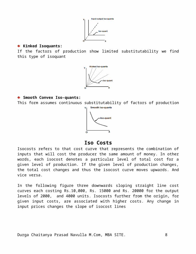
Input-output/ L Shaped Isoquants:If the factors of production are strict complementories and hence show zero substitutability, we derive this isoquant


Kinked Isoquants:If the factors of production show limited substitutability we find this type of isoquant

Smooth Convex Iso-quants:This form assumes continuous substitutability of factors of production

Iso CostsIsocosts refers to that cost curve that represents the combination of inputs that will cost the producer the same amount of money. In other words, each isocost denotes a particular level of total cost for a given level of production. If the given level of production changes, the total cost changes and thus the isocost curve moves upwards. And vice versa.

In the following figure three downwards sloping straight line cost curves each costing Rs.10,000, Rs. 15000 and Rs. 20000 for the output levels of 2000, and 4000 units. Isocosts further from the origin, for given input costs, are associated with higher costs. Any change in input prices changes the slope of isocost lines

Marginal Rate of Technical Substitution(MRTS)The marginal rate of technical substitution refers to the rate at which one input factor is substituted with other to attain a given level of output. In other words, the lesser units of one input must be compensated by increasing amount of another input to produce the same level of output. In the following table


presents the ratio of MRTS between the two input factors, say capital and labour. 7 units of decrease in labour are compensated by an increase in 1 unit of capital, resulting in a MRTS of 7:1.otherwise we can use the following formula.

MRTS= Change∈one inputChange∈another input

Combination

s

inputs Units

MRTSK L

A 1 30 -B 2 23 7:1C 3 18 5:1D 4 15 3:1E 5 13 2:1F 6 12 1:1

Least Cost Combination of InputsThe isocosts curve indicates the alternative combinations of various factors of production which can produce a given output. Of these, an entrepreneur would like to choose the combination of input factors, which costs him the least. To explain this how he can determine the least cost combination for a given output. We need the prices of the factors of production. Let the price of labour (L) be Rs.6 per unit and price of capital (K) Rs.9 per unit. Assume that any amount of labour and capital can be bought at these respective fixed prices.

Let our farmer wants to produce a certain amount of paddy. Assume that the farmer has certain cost combination. There are two ways to determine the least cost combination of input for given output. In the following example there are six alternative combinations of labour and capital to produce the given production, say 9 quintals. The cost of each of these combinations will be as follows

Combination

s

inputs UnitsCostRs.K L

1 1 20 1*9 + 20*6=1292 2 15 2*9 + 15*6=1083 3 11 3*9 + 11*6=844 4 9 4*9 + 9*6=905 5 6 5*9 + 6 * 6=816 6 5 6*9 + 5* 6=84

From the above table we can find the combination of 5 represents the least cost for producing the desired production. The least total cost producing various other quantities can be determined in a similar way.


Graphically we can determine the least cost input combination or the maximum output for given cost, first we have to draw iso-quant map and than iso-costs map. Later we have super-impose the iso-quants map and the iso-costs map as shown in figure.

As per the above figure the desired quantity of output can be produced at a least cost Rs.81 by having 5 units of capital and 6 units of labour. It is known by the point E where the isoquant curve is just tangent to the iso-cost curve. At any other point of iso-quant the total cost is more than Rs.81. similarly for a given cost, an entrepreneur can select the best combination of two inputs which will give the maximum output by way of selecting that iso-quant curve which is just tangent to a given iso-cost curve.

Laws of ReturnsProduction function shows the relationship between the quantity of inputs and the possible output. But the laws of production deal with the relationship in the form of two categories. They are short run production function and long run production function. Short run production function is divided into two categories. They are production function with one variable (Law of Variable Proportion) and production function with two variables (Iso-Quants).

Law of Diminishing Return Or Law of Variable ProportionThe law of variable proportions which is a new name given to old classical concept of “Law of diminishing returns has played a vital role in the modern economics theory. Assume that a firms production function consists of fixed quantities of all inputs (land, equipment, etc.) except labour which is a variable input when the firm expands output by employing more and more labour it alters the proportion between fixed and the variable inputs. The law can be stated as follows:

“When total output or production of a commodity is increased by adding units of a variable input while the quantities of other inputs are held constant, the increase in total production becomes after some point, smaller and smaller”.

The law of variable proportion explains the input- output relation, the change in output due to addition of one variable input. This is a short run phenomenon. The short run is a period in which at least one input is fixed. Thus in the short-run, the increase in production is possible only by increasing the variable inputs. Variation is made only in one factors keeping the other factors fixed, the proportion


between the fixed factors and the variable factors is varied. Hence the study is called the law of variable proportion.

The law also brings diminishing tendency in production is also known as the law of diminishing returns. It states that when at least one factor of production is fixed or factor input is fixed and when all other factors are varied, the total output in the initial stages will increase at an increasing rate, and after reaching certain level of output the total output will increase at declining rate. If variable factor inputs are added further to the fixed factor input, the total output may decline. This Law of Returns is also called The Law of Variable proportions or The Law of Diminishing Returns

Labour TP AP MP Stages

0 0 0 0 Stage I1 10 10 102 26 13 163 36 12 10 Stage II4 44 11 85 48 9.6 46 50 8.3 27 50 7.1 0 Stage

III8 47 5.87 –3TP = Total Production

AP =Average Production (TP÷ Labour )

MP= Marginal Production

ΔTPΔLabour

Here both Average production and marginal production first rise reaches maximum and then decline. The total production increase at increasing rate till the employment of the 4th worker.

After that total product increase at a decreasing rate till 6th worker. The employment of 7th worker will not add any production and thereafter any addition of worker will result in decrease in total product. This is what shown in marginal products. From the above first output is an increasing rate, then increases at decreasing rate and finally decreases. The following diagram explains three stages of diminishing returns. In first state total production increases at a increasing rate. The marginal product in this stage increase at an increasing rate resulting a greater increase in total production. The average product also increases. This stage continuous up to the point where average product is equal to marginal product. The law of increasing returns is in operation till this state.


Diminishing returns starts from the second state onwards. In this stage total product increases only at a diminishing rate. The average product also decline. The second stage comes to an end where total product becomes maximum and marginal product becomes zero. The marginal production becomes negative in the third stage. So the total product also decline. The average product continues to decline.

Assumptions:The production technology unchangedHomogeneous Variable Factor unitsThe fixed factor is indivisible

The production technology unchanged:It is assumed that there is no improvement in technology. If an improved technology is adopted then the increase in returns may be more than proportionate mix.

Homogeneous Variable Factors unit:The law assumes that all the units of the variables factor are identical and exactly similar to each other. Otherwise output may be increase

The fixed Factor is indivisible:The fixed factor remains constant. Its capacity cannot be divided and used for some other proportion

Cause for Operation of the Law of Diminishing ReturnsWrong Combinations of inputs will give Diminishing returnsScarcity of Certain factors like land and capital in the short run will give diminishing marginal productivity of the variable factorImperfect substitutes also give diminishing returns

Laws of ReturnsProduction function shows the relationship between the quantity of inputs and the possible output. But the laws of production deal with the relationship in the form of

Law of returns to scaleLaw of variable proportion/ Law of diminishing returns/ law of returns

Law of Return to ScaleIn the long run all the factors of production are variable and an increase in output is possible by increasing all the inputs. Returns to scale implies the change in output or returns when all factors are


change simultaneously in same ratio. In this law all the factors of production are changed in the same ratio.

There are three laws of returns governing production function. They areLaw of Increasing Returns to ScaleLaw of Constant Returns to ScaleLaw of Decreasing Returns to Scale

1. Law of Increasing Returns to ScaleThis law states that the volume of output keeps on increasing with every increase in the input. Where given increase in factors of production results in a more than proportionate increase in output. In this first stage of production, the marginal output increases. It will explain through the following

Pr oportionate Change in OutputPr oportionate Change in Input

>1

Causes for Increasing ReturnsIndivisible factorsScope for greater specializationAdvantage of increasing dimensionsExternal economies

1. Indivisible factors:Some factors of production are available only in a certain minimum size. E. g. Suppose we have installed an electricity generating plant capable of producing one million K.W. power, even though the needs of the town is only 5000 K.W. because it id the smallest size available. The capacity may not be utilized fully. Demand for electricity may be increased. With same plant we can produce more. No additional expenditure on plant and machinery is required. Thus, we get increasing returns where there are indivisible factors.

2. Scope for greater specialization:When the scale of production is increased, there is scope for introduction greater specialization of labour and equipment. Work can be divided into small tasks. It increases efficiency of the factors resulting in increasing returns.

3. Advantages of increasing dimensionsIncreased dimensions give rise to certain economies. E.g. the cost of constructing a double ducker bus is less than that of two single buses. So the cost of operating large and bigger machinery will be less. Thus, the economies of increased dimensions reduce costs and give rise to the law of increasing returns.

4. External Economies:External economies are those that arise when the industry expands. Transport, banking, insurance, Research Facilities etc. develop when the industry expands. Cost of production is reduced.

Law of Constant Returns to ScaleIncreasing returns to scale do not continue indefinitely. As the firm expands production more and more, the advantages of large scale production gradually give place to disadvantages. There is a limit to the advantages of size. At certain size of production the advantages and disadvantages of large scale production balance each other and we get constant result. i.e.



=1

Law of Decreasing Returns to ScaleConstant returns to scale are only a passing phase. If the scale of production is increased further, diminishing returns will se in and the costs of production will rise.


<1

They are Business may becomes unmanageableIndivisible factors may become unmanageableProblems due to supervision control and coordination will arise.

To these internal diseconomies are added external diseconomies will give diminishing returns.

Assumptions:All the factors are variableThere are no technological changesThere is perfect competitionThe output is measured in physical units

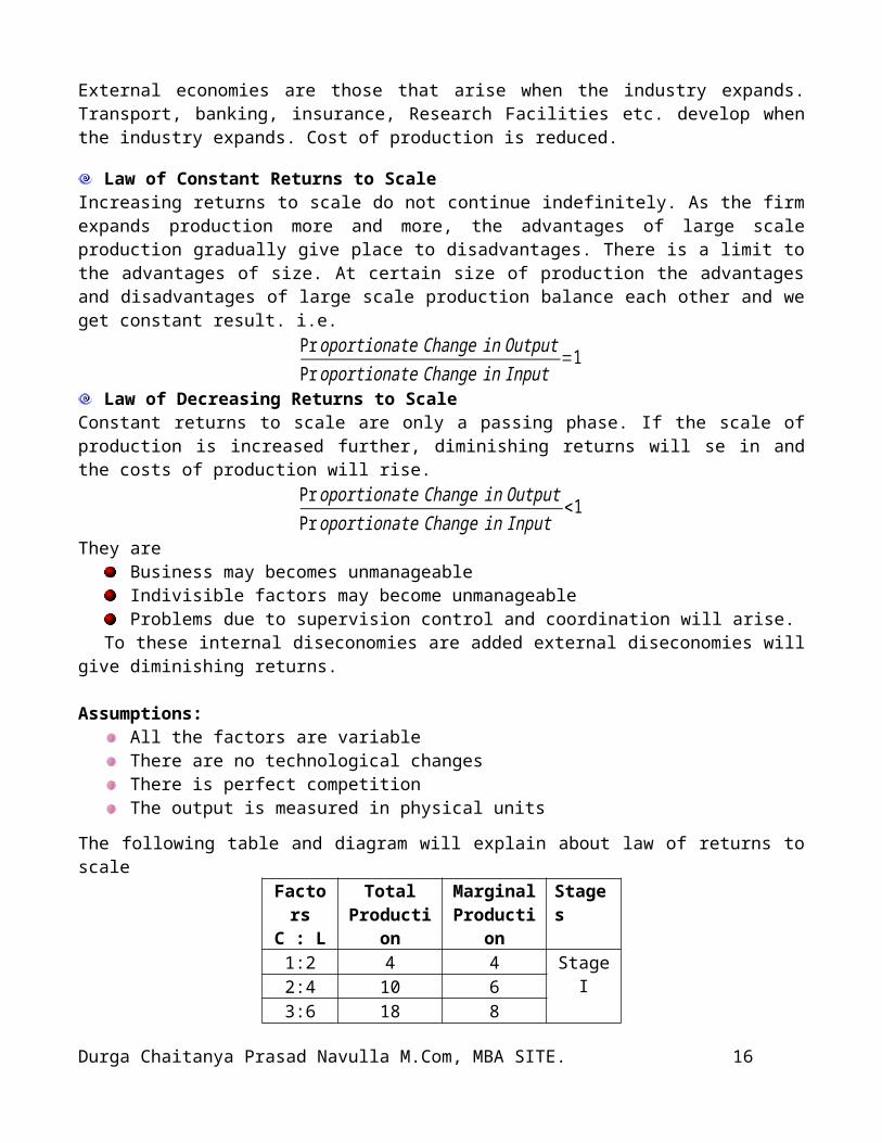
The following table and diagram will explain about law of returns to scaleFactorsC : L

TotalProduction

MarginalProduction

Stages

1:2 4 4Stage

I2:4 10 63:6 18 84:8 28 105:10 38 10 Stage

II6:12 48 107:14 56 8 Stage

III8:16 62 6

In the above table 1 acre of land and 2 labour are employed, the total product sis 4 units of paddy. When the inputs are doubled i.e. 2 acre of land and 4 labour are employed, the output of paddy is more than double i.e. 10 and marginal output goes up from 4 units to 6 units and so on. So in the first stage increasing returns will come.

Increasing returns to scale cannot be experienced by the firm indefinitely. Firms slowly enter the phase of constant returns to scale. When the input factors are increased to 5 acres of land and 10 labour then the marginal out put remain constant. Doubling in all inputs simple results in doubling the output. This is the stage of constant returns.

A firm cannot enjoy increasing returns indefinitely. Sooner or later they reach the stage of decreasing to scale which implies that proportionate increase in all inputs resulting less than proportionate increase in output. This is the third stage or the decreasing returns stage. Every firm experience three phase-increasing returns in the beginning then constant returns for a short period and ultimately decreasing returns to scale.


OX axis shows scale of production. OY axis Output. As the scale of production increases, up to the point C we get Increasing returns. From C to D we get Constant returns. From D onwards we get Diminishing Returns.

Law of Returns to scale are shown separately in the following diagrams in terms of Isoquants

Diagram A shows increasing Returns to scale. The output increases by 100 units from 100 to 200 and 200 to 300. But the distance between the Isoquants shortens. MN is shorter than OM and NP is shorter than MN. It means that for the given increase in output the firm has to devote less factors than before. It implies Increasing Returns

Diagram B shows Constant Returns to scale. The output increases by 100 units. But the distance between the different Isoquants is sameDiagram C shows Diminishing Returns to scale. The output increases by 100 units. But the distance between the different Isoquants is increasing showing that more factors have to be used than before NP is greater than MN

Economies of ScaleProduction may be carried on a small scale or on a large by a firm. When a firm expands its size of production by increasing all the factors, it secures certain advantages known as economies of production. These economies of large scale production have been classified by Marshall in to two kinds they areInternal Economies:Internal Economies are those which are opened to a single factory or a single firm independently of the action of other firms. It is based on the size of the firm and it is different for different firms.Causes for internal economies

1. Indivisibilities2. Specialisation of workers

It may be of following types

Technical EconomiesManagerial Economies


Marketing EconomiesFinancial EconomiesRisk Bearing EconomiesEconomies of ResearchEconomies of WelfareEconomies of By-products

Technical Economies:It may be arise to a firm from the use of better machines and superior techniques of production. As a result, production increases and the per unit cost of production falls. Another technical economy lies in the mechanical advantage is using large machines. Technical economies also be associated when large firm is able to utilize all its waste materials for the development of by-products.

Managerial Economies:A large firm can appoint specialists to supervise and manage the various departments. It increases its productive efficiency. This is a form of division of labour. For example, large-scale manufacturers employ specialists to supervise production systems. And better management; increased investment in human resources and the use of specialist equipment, such as networked computers can improve communication, raise productivity and thereby reduce unit costs.

Marketing Economies:A large fir buys material in bulk. There it can get them at relatively lower prices. It can increase its sales by salesmanship, advertisement attractive packing etc. it can produce quality products. These are also called “Commercial Economies”

Financial Economies:Larger firms are usually rated by the financial markets to be more ‘credit worthy’ and have access to credit facilities with favorable rates of borrowing. In contrast, smaller firms often face higher rates of interest on overdrafts and loans. Businesses quoted on the stock market can normally raise fresh money (extra financial capital) more cheaply through the sale (issue) of equities to the capital market. They are also likely to pay a lower rate of interest on new company bonds because of a better credit rating.

Risk Bearing Economies:A large firm can produce a variety of products. It can sell the products in different markets both within the country and in foreign countries also if the products can be exported. It can purchase the materials from different sources. This is called diversification.

Diversification reduces risks. If more than one commodity is produced,, the loss on one product can be compensated by the profit on the other products. Diversification of production and marketing increases the ability of the firm to withstand losses. It will have greater stability.

Economies of Research:Large firm can establish its own research laboratory and employ trained research workers. It can thus invent new methods of production, new products etc., which will reduce costs and increase scales.

Economies of Welfare:


A large firm can provide better working conditions in and outside the factory. Facilities like subsidized canteens, crèches for the infants, recreation rooms, cheap houses, educational and medical facilities ten to increase the productive efficiency of the workers which helps in raising production and reducing costs

Economies of By-productsLarge firms can make a more economical use of their raw materials. A large firm can avoid waste of its raw material, which it can economically use of manufacturing certain by-products.

External Economies:Business firms enjoys a number of external economies, which are discussed below

Economies of ConcentrationEconomies of informationEconomies of WelfareEconomies of Specilisation

Economies of Concentration:When an industry is concentrated in a particular area, all the member firms reap some common economies like skilled labour, improved means of transport and communications, banking and financial services etc. all these factors felicities tend to lower the unit cost of production.

Economies of Information:Information centre can be set up be large organizations which can publish a journal and passes on the information to the firms regarding the availability of raw materials, modern machines, export possibilities etc. this would help the firms in raising the productive efficiency

Economies of Welfare:Housing colonies, educational institutions, hospitals, recreation facilities etc, can be provided to the workers by the industry, it would improve efficiency of the workers and every firm benefits from it

Economies of Specialisation:The firms in the industry can specialize in one variety of the product or in one stage of production. Such vertical and lateral specialisation reduces the costs of production of the firms and improvement of quality. Thus internal economies depend upon the size of the firm and external economies depend upon the size of the industry.


Cost AnalysisCost analysis deals with the behaviour of cost. In other words cost analysis is concerned with financial aspect of production relations as against physical considered in production analysis. Therefore cost analysis refers to the study of behaviour of cost in relation size of out-put, scale of operation, price of factors of production and other related economic variables. Cost refers to the amount of expenditure incurred in acquiring something. In business firm it refers to the expenditure incurred to produce an output or provide service. Thus the cost incurred in connection with raw material, labour, other heads constitute the overall cost of production. A managerial economist must have a clear understanding of the different cost concepts for clear business thinking and proper application. Output is an important factor which influences the cost.

The cost-output relationship plays an important role in determining the optimum level of production. The knowledge of the cost output relation helps the manager in cost control, profit, production, pricing, promotion etc. the relation between cost and its determinants explained through the following function

C =∫(S , O , P , T )Where C= CostS= Size of Plant / Scale of operationO= Output levelP= Prices of inputsT= Technology

As per the formula, as the size of the plant increases, the economies of scale start following and hence the cost per unit will come down. Similarly, an increase in output results in increase in cost and vice versa. Apart from output, prices of inputs represent a positive relationship with cost of production. As we know, a sophisticated technology may reduce cost compared to outdated technology lasty, managerial efficiency also has a bearing on cost of production.

Cost Concepts:The various relevant concepts of costs used in business decisions are discussed below. Opportunity Costs and Outlay Cost Explicit and Implicit/ Imputed Cost Historical Cost and Replacement Cost Short Run and Long run Costs Out of Pocket and Book Costs Fixed Cost and Variable Costs Past and Future Costs Traceable Cost and Common Costs Avoidable Costs and Unavoidable Costs Controllable Cost and Uncontrollable Cost Incremental Cost and Suck Costs Total, Average and Marginal Costs Accounting and Economic Costs

They are Opportunity Costs and Outlay Cost:


Out lay costs, also known as actual costs or absolute costs. These are the payments made for labour, material, plant, transportation etc. All these are appearing in the books of accounts.

Opportunity cost implies the earning foregone on the next best alternative has the present option been undertaken. This cost is often measured by assessing the alternative which has to be sacrificed if the particular line is followed.

Ex. A business man is able to borrow certain amount at 10% to buy a machine. Instead of buying the machine he can reinvest the borrowed fund at say 12%. In this situation, the opportunity cost is said to be 12% and outlay cost 10%.

Explicit and Implicit/ Imputed Cost Explicit costs are those expenses that involve cash payments. These are the actual or business costs

that appear in the books of accounts. Explicit cost is the payment made by the employer for those factors of production hired by him from outside.E.g. Wages, Salaries paid, payments for raw materials, interest on borrowed capital fundsImplicit costs are the costs of the factor units that are owned by the employer himself. It does not involve cash payment and hence does not appear in the books of accounts. These costs are not actually incurred but would have been incurred in the absence of employment of self-owned factors.

Historical Cost and Replacement Cost Historical cost is the original cost of an asset. Historical cost valuation shows the cost of an asset paid originally when the asset was acquired in the past. Historical valuation is the basis for financial accounts. Replacement cost is the price that would have to be paid currently to replace the same asset.

E.g The price of a machine at the time of purchase was Rs. 17,000 and the present price of the machine is Rs. 20,000 is the replacement cost.

Short Run and Long run Costs: Time is another variable for cost distinction. Short-run is a period during which the physical capacity of the firm remains fixed. Any increase in output during this period is possible only by using the existing physical capacity more intensively. But in the long run it is possible to change the firm’s physical capacity as all the input are variable including plant and capital equipment.

Out of Pocket and Book Costs:

Out of pocket costs, also known as explicit costs, are those costs that involve current payments. E.g, wages, rent, interest etc.

But the book costs are taken into account in determining the legal dividend payable during a period. Both are considered for all decisions.

Fixed Cost and Variable Costs: Fixed cost is that cost which remains constant for certain level of output. It is not changed by the changes in the volume of production. But fixed cost per unit decrease, when the production is increased. E.g. salaries, rent on factory and depreciation on machinery etc.

Variable cost is that which varies directly with the variation in output. An increase in total output results in an increase in total variable costs and decrease in total output results in a proportionate decline in the total variable costs .E.g Materials, direct labour expenses, and Routine maintenance expenditure.


Past and Future Costs: Past Costs also called historical costs, are the actual costs incurred and recorded in the books of

accounts. These costs are useful only for evaluation and not for decision making.

Future costs are costs that are expected to be incurred in the future. They are not actual costs. They are the costs forecast or estimated with rational methods.

Traceable and Common Costs: Traceable cost, otherwise called direct cost, is one which can be identified with a production process or product. Raw material, labour involved in production are examples of traceable cost.

Common Costs are the costs are the ones that cannot be attributed to a particular process or product. It can not be directly identified with any particular process or type of product.

Avoidable Costs and Unavoidable Costs: Avoidable costs are the costs which can be reduced if the business activities of a concern are reduced. E.g. if some workers can be retrenched with a drop in a product-line, or volume or production, the wages of the retrenched workers are escapable costs.

The unavoidable costs are otherwise called sunk costs. There will not be any reduction in this cost even if reduction in business activity is made. E.g when the volume of production is reduced from 8,000 units to 5,000 units the present machines has some idle capacity. It cannot be unavoidable cost.

Controllable Cost and Uncontrollable Cost:

Controllable costs are the ones which can be regulated by the executive who is in charge of it. It is based on levels of management.

Some costs are not directly identifiable with a process of product. They are appointed to various processes or products in some proportions. These costs are called uncontrollable costs.

Incremental Cost and Suck Costs: Incremental cost also known as differential cost is the additional cost due to a change in the level or nature of business activity. The change may be caused by adding a new product, adding new machine, replacing a machine by a better one etc.

Sunk costs are those which are not altered by any change. They are the costs incurred in the past. This cost is the result of past decision and cannot be changed by future decisions. Once an asset has been bought or an investment made, the funds locked up represent sunk costs.


Total, Average and Marginal Costs: Total cost is the cash payment made for the input needed for production. It may be explicit or implicit. It is the sum total of fixed and variable costs. Average cost is the cost per unit of output. It is obtained by dividing the total cost by the total quantity produced.

Average Cost =

TCQ

Marginal cost is the additional cost incurred to produce an additional unit of output. In other words, it is the cost of the marginal unit produced.

Accounting and Economic Costs Accounting costs are the costs recorded for the purpose of preparing the balance sheet and profit and loss statements to meet the legal, financial and tax purpose of the company.Economic concept considers future costs and future revenues which help future planning and choice.

These costs are used on the basis of management requirements for decision making.


BEP ANALYSISIntroduction:Profit maximisation is one of the major goals of any business. The other goals include enlarging the customer base, entering new markets, innovation through major investments in research and development and so on. The volume of profit is determined by a number of internal and external factors. As a part of monitoring the profitability of the operations of the business, it is necessary for the managerial economist to study the impact of changes in the internal factors such as cost, price and volume on profitability, breakeven analysis comes very handy of these purpose.Break-even analysis refers to analysis of the break-even point (BEP). The BEP is defined as a no-profit or no-loss point. Why is it necessary to determine the BEP when there is neither profit nor loss? It is important because it denotes the minimum volume of production to be undertaken to avoid losses. In other words, it denotes the minimum volume of production to be undertaken to avoid losses. In other words, it points out how much minimum is to be produced to see the profits. It is a technique for profit planning and control, and therefore is considered a valuable managerial tool.Break – even analysis is defined as analysis of costs and their possible impact on revenues and volume of the firm. Hence, it is also called the cost-volume –profit analysis. But there is slight difference between the two. CVP analysis is broader and it includes the entire planning for profit, while Break Even Analysis is a technique used in this process. But we used these two terms as interchangeable words. A firm is said to attain the (BEP) when its total revenue is equal to total cost (TR = TC)Total cost comprises fixed cost and variable cost. The significant variables on which the BEP is based fixed cost, variable cost and total revenue.

Assumptions Underlying Break-even Analysis:The following are the assumptions underlying break-even analysis:

a) Costs can be classified into fixed and variable costs.b) Total fixed cost remains constant at all levels of outputc) Variable cost is varies on the basis of outputd) Selling price does not change with volume changes. It remains fixed. It does not consider the

price discounts or cash discounts.e) All the goods produced are sold. There is no closing stock.f) There is only one product available for sale. g) In case of multi-product firms, the product mix does not change.


Significance of BEA:Break-even analysis is a valuable tool

To ascertain the profit on a particular level of sales volume or a given capacity of production To calculate sales required to earn a particular desired level of profit To compare the product lines, sales area,, methods of sale for individual company To compare the efficiency of the different firms To decide whether to add a particular product to the existing product line or drop one from it To decide to ‘make or buy’ a given component or spare part To decide what promotion mix will yield optimum sales To assess the impact of changes in fixed cost, variable cost or selling price on BEP and profits

during a given period

Limitations of Break-Even Analysis:Break-even analysis has certain underlying assumptions which form its limitations

Break-even point is based on fixed cost, variable cost and total revenue. A change in one variable is going to affect the BEP.

All costs cannot be classified into fixed and variable cost. We have semi-variable costs also. Incase of multi-product firm, a single chart cannot be of any use. Series of charts have to be made use of.

In case of multi-product firm, a single chart cannot be of any use. Series of charts have to be made use of.

This analysis is useful in short run not in long run. Total cost and total revenue lines are not always straight as shown in the figure. The quantity and

price discounts are the usual phenomena affecting the total revenue line. Where the business conditions are volatile. BEP cannot give stable results.

--------S=V+F+P, V=S-F-P, F=S-V-P, P=S-V-F, S-V=C, F+P=CWhere

S= Sales V= Variable Cost F= Fixed Cost P= Profit C= Contribution

BEP(Units )= FS−V

BEP( Sales) = BEP Units∗ Selling Pr ice Per Unit

BEP( Sales) = FPV Ratio


Margin of SafetyMargin of safety is the excess of sales over the break even sales. It can be expressed in percentage or in absolute sales amount. A large margin of safety indicates the soundness of the business the formulate for the margin of safety is

M arg in Of Safety = Total Sales −BEP Sales (or)M arg in of Safety ( Sales) = P

PV Ratio

Angle of Incidence:This is the angle between sales line and total cost line at the break even point. It indicates the profit earning capacity of the concern. Large angle of incidence indicate a high rate of profit, a small angle indicates a low rate of earnings. To improve this angle, contribution should be increased either by raising the selling price by reducing variable cost.

PV Ratio:Profit Volume ration is usually called PV ratio. It is one of the most useful ratios for studying the profitability of business. The ration of contribution to sales is the P.V ration. It may express in percentage. The organisation increased the P. V ratio by increasing the selling price per unit or buy reducing the variable cost. The formulas are

PV Ratio = S−VS

∗ 100 (or)

PV Ratio = CS∗ 100

(or) PV Ratio = F+P

S∗ 100

PV Ratio = Change in Pr ofitChange in Sales

∗ 100

Desired Sales = F+PPV Ratio

Problem1:

Find Break Even Point in Units and BEP sales through the followFixed Cost=1,50,000Variable Cost=Rs. 15Selling Price per unit =20/-Solution:

BEP Units = ¿Cost

Selling Price Per unit−VariableCost Per unit

BEP Units = 1,50,00020−15

BEP Units = 30,000BEP Sales= BEP units X Selling Price Per UnitBEP Sales= 30,000 X 20BEP Sales= 6,00,000/-


Problem 2:A company prepares a budget to produce 3,00,000 units with fixed cost Rs. 15,00,000/- Variable cost is Rs.10/- per unit Profit is 20% on Total Cost. Calculate BEP

Solution:Total Units=3,00,000Fixed Cost =15,00,000/-Variable Cost= 3,00,000 X 10 =30,00,000Profit = 20% on Total Cost

Total Cost = Fixed Cost + Variable CostTotal Cost = 15,00,000+30,00,000Total Cost=45,00,000

Profit= 45,00,000 X (20/100)Profit=9,00,000/-

Sales= Fixed Cost + Variable Cost + ProfitSales=15,00,000+ 30,00,000 + 9,00,000Sales=54,00,000/-

Selling Price per Unit = Total Sales / Total Produced UnitsSelling Price per Unit = 54,00,000 / 3,00,000Selling Price per Unit = 18/-

BEP Units = ¿Cost

Selling Price Per unit−Variablecos t Perunit

BEP Units = 15,00,000

18−10

BEP Units = 1,87,500

BEP Sales = BEP Units X Selling Price Per UnitBEP Sales = 1,87,500 X 18 = Rs. 33,75,000/-

Problem: 3From the following information you are required to calculate

1) P.V Ratio 2) BEP Sales 3) Margin of SafetySales= Rs. 40,000/- Variable Cost = 20,000/- Fixed Cost = 16,000/-

1). P.V Ratio:

P .V . Ratio=Sales−VariableCostSales

X 100


P .V . Ratio=40,000−20,00040,000

X100

P .V . Ratio=50 %2). BEP Sales:

BEP Sales= ¿CostP.V .Ratio

BEP Sales=16,0000.5

BEP Sales=32,000 /−¿3) Margin of Safety:

BEP Sales=Total Sales−BEPSales

BEP Sales=40,000−32,000

BEP Sales=8,000 /−¿

Problem 4:Determine P.V. Ratio and Fixed Cost and BEP Sales from the following information

Particulars I period II PeriodSales 1,00,000 1,40,000Profit 4,000 12,000

1). P.V Ratio:

P .V . Ratio=Change∈ProfitChange∈Sales

X100

P .V . Ratio= 8,00040,000

X 100

P .V . Ratio=20 %∨0.2

II) Fixed Cost: For finding fixed cost take any period data as base.

Desire Sales= F+PP .V .Ratio

1,00,000=F+4,0000.2

1,00,000 X 0.2=F+4,000F=20,000−4,000F=16,000/−¿


II) BEP Sales:


BEP Sales=16,000/−¿0.2

¿

BEP Sales = Rs. 80,000/-

Problem:5The following figures of Sales and Profit of two periods are available in respect of firm

Particulars I period II PeriodSales 10,00,000 12,00,000Profit 1,50,000 2,30,000

You are required to calculate1. P.V ratio 2. BEP Sales 3.Sales required to earn profit of Rs. 20,000/- 4. Profit of estimated sales of Rs. 1,50,000/-5. Margin of Safety at a profit of Rs. 50,000

1) P.V ratio:

P .V . Ratio=Change∈ProfitChange∈Sales

X100

P .V . Ratio= 80,0002,00,000

X 100

P .V . Ratio=4 0 %∨0.42) BEP Sales: Fixed Cost: For finding fixed cost take any period data as base.


10,00,000=F+1,50,0000.4

10,00,000 X 0.4=F+1,50,000F=4,00,000−1,50,000

F=2,50,000/−¿


BEP Sales=2,50,000/−¿0.4

¿

BEP Sales = Rs. 6,25,000/-


3. Sales required to earn profit of Rs. 2,00,000/-


Desire Sales=6,25,000+2,00,0000.4

Desire Sales=20,62,500

4. Profit of estimated sales of Rs. 50,00,000/-


50,00,000=6,25,000+P0.4

50,00,000 X 0.4=6,25,000+P

P=13,75,000/-

5. Margin of Safety at a profit of Rs. 5,00,000/-

Marginof Safety= ProfitP.V .Ratio

Marginof Safety=5,00,0000.4

Marginof Safety=¿12,50,000/-

Problem:6If sales are 10,000 units and selling price is Rs. 20/- per unit, variable coast Rs. 10/- per unit, fixed cost Rs. 80,000/-. Find out BEP and BEP Sales. Calculate profit earned. What should be the sales for earning a profit of Rs. 60,000/- (JNTU Apr./May 2004)

Solution:BEP (Units)

BEP Units = ¿Cost

Selling Price Per unit−Variablecos t Perunit

BEP Units = 80,00020−10

BEP Units = 8,000 units


BEP Sales:BEP Sales = BEP Units X Selling Price Per unit

BEP Sales= 8,000 X 20BEP Sales=1,60,000/-

Profit earned:Profit = Sales – Variable Cost – Fixed Cost

Profit= 2,00,000 – 1,00,000 - 80,000Profit = 20,000/-

What should be the sales for earning a profit of Rs 60,000/-


Desire sales=80,000+60,0000.5

Desire Sales=2,80,000 /−¿

P=13,75,000/-

P .V . Ratio=Sales−VariableCostSales

X 100

P .V . Ratio=20−1020

X 100

P .V . Ratio=50 %∨0.5


Date post:	07-Aug-2015
Category:	Education
Upload:	chaitanya-prasad
View:	60 times
Download:	7 times

MEFA II UNIT COMPLETE NOTES

Education