An optimal three-point eighth-order iterative method without

memory for solving nonlinear equations with its dynamics

Gunar Matthies a∗ Mehdi Salimi b,c† Somayeh Sharifi d‡

Juan Luis Varona e§

aInstitut fur Numerische Mathematik, Technische Universitat Dresden, GermanybCenter for Dynamics, Department of Mathematics, Technische Universitat Dresden, Germany

cDepartment of Mathematics, Universiti Putra Malaysia, 43400 UPM Serdang, Selangor, MalaysiadMEDAlics, Research Center at Universita per Stranieri Dante Alighieri, Reggio Calabria, Italy

eDepartamento de Matematicas y Computacion, Universidad de La Rioja, Logrono, Spain

Abstract

We present a three-point iterative method without memory for solving nonlinear equations inone variable. The proposed method provides convergence order eight with four function evalua-tions per iteration. Hence, it possesses a very high computational efficiency and supports Kungand Traub’s conjecture. The construction, the convergence analysis, and the numerical imple-mentation of the method will be presented. Using several test problems, the proposed methodwill be compared with existing methods of convergence order eight concerning accuracy and basinof attraction. Furthermore, some measures are used to judge methods with respect to their per-formance in finding the basin of attraction.

Keywords: Optimal multi-point iterative methods; Simple root; Order of convergence; Kungand Traub’s conjecture; Basins of attraction.

Mathematics Subject Classification: 65H05, 37F10

1 Introduction

Solving nonlinear equations is a basic and extremely valuable tool in all fields in science and engineer-ing. One can distinguish between two general approaches for solving nonlinear equations numerically,namely, one-point and multi-point methods. The basic optimality theorem shows that an analyticone-point method based on k evaluations is of order at most k, see [27, § 5.4] or [15] for an improved

proof. The Newton–Raphson method xn+1 := xn − f(xn)f ′(xn)

is probably the most widely used algo-

rithms for finding roots. It requires two evaluations per iteration step, one for f and one for f ′, andresults in second order convergence which is optimal for this one-point method.

Some computational issues encountered by one-point methods are overcome by multi-point meth-ods since they allow to achieve greater accuracy with the same number of function evaluations. Im-portant aspects related to these methods are convergence order and efficiency. It is favorable to attainwith a fixed number of function evaluations per iteration step a convergence order which is as high aspossible. A central role in this context plays the unproved conjecture by Kung and Traub [15] whichstates that an optimal multi-point method without memory provides a convergence order of 2k while

∗gunar.matthies@tu-dresden.de†mehdi.salimi@tu-dresden.de‡somayeh.sharifi@medalics.org§jvarona@unirioja.es

1

arX

iv:1

602.

0702

6v1

[m

ath.

NA

] 2

3 Fe

b 20

16

using k + 1 evaluations in each iteration step. The efficiency index for a method with k evaluationsand convergence order p and k evaluations is given by E(k, p) = k

√p, see [19]. Hence, the efficiency

of a method supporting Kung and Traub’s conjecture isk+1√

2k. In particular, an optimal methodwith convergence order eight has an efficiency index 4

√8 ' 1.68179.

A large number of multi-point methods for finding simple roots of a nonlinear equation f(x) = 0with a scalar function f : D ⊂ R → R which is defined on an open interval D (or f : D ⊂ C → Cdefined on a region D in the complex plane C) have been developed and analyzed for improving theconvergence order of classical methods like the Newton–Raphson iteration.

Some well known two-point methods without memory are described e.g. in Jarratt [13], King [14],and Ostrowski [19]. Using inverse interpolation, Kung and Traub [15] constructed two general optimalclasses without memory. Since then, there have been many attempts to construct optimal multi-pointmethods, utilizing e.g. weight functions, see in particular [2, 3, 5, 16,20–24,26,29].

We will construct a three-point method of convergence order eight which is free from second orderderivatives, uses 4 evaluations, and provides the efficiency index 4

√8 ' 1.68179.

A wide used criterion to judge and rank different methods for solving nonlinear equations is thebasin of attraction. We will use two measures to assess the performance in finding the basin ofattraction [28].

The paper is organized as follows. Section 2 introduces the new methods based on a Newtonstep and Newton’s interpolation. Moreover, details of the new method and the proof of its optimalconvergence order eight are given. The numerical performance of the proposed method compared toother methods are illustrated in Section 3. We approximate and visualize the basins of attraction inSection 4 for the proposed method and several existing methods, both graphically and by mean ofintroduced numerical performance measures [28]. Finally, we conclude in Section 5.

2 Description of the method and convergence analysis

We construct in this section a new optimal three-point method for solving nonlinear equations byusing a Newton-step and Newton’s interpolation polynomial of degree three which was also appliedin [22].

Method 1: The new method is given by

yn := xn − un(xn),

zn := xn − un(xn)

(1 +

f(yn)

f(xn)+

(1 +

1

1 + un(xn)

)(f(yn)

f(xn)

)2),

xn+1 := zn −f(zn)

f [zn, yn] + (zn − yn)f [zn, yn, xn] + (zn − yn)(zn − xn)f [zn, yn, xn, xn],

(2.1)

where un(xn) = f(xn)f ′(xn)

. The standard notation for divided differences in Newton’s interpolation

g[tν , tν+1, . . . , tν+j ] =g[tν+1, . . . , tν+j ]− g[tν , . . . , tν+j−1]

tν+j − tν,

with g[tν ] = g(tν) and g[tν , tν ] = g′(tν) are used.The iteration method (2.1) and all forthcoming methods are applied for n = 0, 1, . . . where x0

denotes an initial approximation of the simple root x∗ of the function f . The method (2.1) uses fourevaluations per iteration step, three for f and one for f ′. Note that (2.1) works for real and complexfunctions.

The convergence order of method (2.1) is given in the following theorem.

2

Theorem 1. Let f : D ⊂ R → R be an eight times continuously differentiable function with asimple zero x∗ ∈ D. If the initial point x0 is sufficiently close to x∗ then the method defined by (2.1)converges to x∗ with order eight.

Proof. Let en := xn−x∗, en,y := yn−x∗, en,z := zn−x∗ and cn := f (n)(x∗)n! f ′(x∗) for n ∈ N. Using the fact

that f(x∗) = 0, the Taylor expansion of f at x∗ yields

f(xn) = f ′(x∗)(en + c2e

2n + c3e

3n + · · ·+ c8e

8n

)+O(e9n) (2.2)

andf ′(xn) = f ′(x∗)

(1 + 2c2en + 3c3e

2n + 4c4e

3n + · · ·+ 9c9e

8n

)+O(e9n). (2.3)

Therefore, we have

f(xn)

f ′(xn)= en − c2e2n +

(2c22 − 2c3

)e3n +

(−4c32 + 7c2c3 − 3c4

)e4n

+(8c42 − 20c22c3 + 6c23 + 10c2c4 − 4c5

)e5n

+(−16c52 + 52c32c3 − 28c22c4 + 17c3c4 − c2(33c23 − 13c5)

)e6n +O(e7n),

and

en,y = yn − x∗ = c2e2n +

(−2c22 + 2c3

)e3n +

(4c32 − 7c2c3 + 3c4

)e4n

+(−8c42 + 20c22c3 − 6c23 − 10c2c4 + 4c5

)e5n

+(16c52 − 52c32c3 + 28c22c4 − 17c3c4 + c2(33c23 − 13c5)

)e6n +O(e7n).

We havef(yn) = f ′(x∗)

(en,y + c2e

2n,y + c3e

3n,y + · · ·+ c8e

8n,y

)+O(e9n,y) (2.4)

by a Taylor expansion of f at x∗. By substituting (2.2)–(2.4) into (2.1), we get

en,z = zn − x∗ = c2(c2 + 5c22 − c3

)e4n

+(−8c32 − 36c42 − 2c23 + c22(−1 + 32c3) + c2(4c3 − 2c4)

)e5n +O(e6n).

We obtainf(zn) = f ′(x∗)

(en,z + c2e

2n,z + c3e

3n,z + · · ·+ c8e

8n,z

)+O(e9n,z) (2.5)

by using again a Taylor expansion of f at x∗. Substituting (2.2)–(2.5) into (2.1), we get

en+1 = xn+1 − x∗ = c22(c2 + 5c22 − c3

) (c22 − 5c32 − c2c3 + c4

)e8n +O(e9n), (2.6)

which finishes the proof of the theorem.

We will compare the new method (2.1) with some existing optimal three-point methods of ordereight having the same optimal computational efficiency index equal to 4

√8 ' 1.68179, see [19,27].

The existing methods that we are going to use to compare are the following:

Method 2: The method by Chun and Lee [5] is given by

yn := xn −f(xn)

f ′(xn),

zn := yn −f(yn)

f ′(xn)· 1(

1− f(yn)f(xn)

)2 ,xn+1 := zn −

f(zn)

f ′(xn)· 1

(1−H(tn)− J(sn)− P (un))2

(2.7)

3

with weight functions

H(tn) = −β − γ + tn +t2n2− t3n

2, J(sn) = β +

sn2, P (un) = γ +

un2,

where tn = f(yn)f(xn)

, sn = f(zn)f(xn)

, un = f(zn)f(yn)

, and β, γ ∈ R. Note that the parameters β and γ cancel

when used in (2.7). Hence, their choice has no contribution to the method.

Method 3: The method by B. Neta [17], see also [18, formula (9)], is given by

yn := xn −f(xn)

f ′(xn),

zn := yn −f(xn) +Af(yn)

f(xn) + (A− 2)f(yn)· f(yn)

f ′(xn), A ∈ R,

xn+1 := yn + δ1f2(xn) + δ2f

3(xn),

(2.8)

where

Fy = f(yn)− f(xn), Fz = f(zn)− f(xn),

ζy =1

Fy

(yn − xnFy

− 1

f ′(xn)

), ζz =

1

Fz

(zn − xnFz

− 1

f ′(xn)

),

δ2 = − ζy − ζzFy − Fz

, δ1 = ζy + δ2Fy.

We will use A = 0 in the numerical experiments of this paper.

Method 4: The Sharma and Sharma method [24] is given by

yn := xn −f(xn)

f ′(xn),

zn := yn −f(yn)

f ′(xn)· f(xn)

f(xn)− 2f(yn),

xn+1 := zn −f [xn, yn]f(zn)

f [xn, zn]f [yn, zn]W (tn),

(2.9)

with the weight function

W (tn) = 1 +tn

1 + αtn, α ∈ R,

and tn = f(zn)f(xn)

. We will use α = 1 in the numerical experiments of this paper.

Method 5: The method from Babajee, Cordero, Soleymani and Torregrosa [2] is given by

yn := xn −f(xn)

f ′(xn)

(1 +

(f(xn)

f ′(xn)

)5),

zn := yn −f(yn)

f ′(xn)

(1− f(yn)

f(xn)

)−2,

xn+1 := zn −f(zn)

f ′(xn)·

1 +

(f(yn)

f(xn)

)2

+ 5

(f(yn)

f(xn)

)4

+f(zn)

f(yn)(1− f(yn)

f(xn)− f(zn)

f(xn)

)2 .

(2.10)

4

Method 6: The method from Thukral and Petkovic [26] is given by

yn := xn −f(xn)

f ′(xn),

zn := yn −f(yn)

f ′(xn)· f(xn) + βf(yn)

f(xn) + (β − 2)f(yn), β ∈ R,

xn+1 := zn −f(zn)

f ′(xn)· (ϕ(tn) + ψ(sn) + ω(un)) ,

(2.11)

where weight functions are

ϕ(tn) =

(1 +

tn1− 2tn

)2

, ψ(sn) =sn

1− αsn, α ∈ R, ω(un) = 4un,

and tn = f(yn)f(xn)

, sn = f(zn)f(yn)

and un = f(zn)f(xn)

. We will use β = 0 and α = 1 in the numerical experimentsof this paper.

3 Numerical examples

The new three-point method (2.1) is tested on several nonlinear equations. To obtain high accuracyand avoid the loss of significant digits, we employed multi-precision arithmetic with 20 000 significantdecimal digits in the programming package Mathematica.

We are going to perform numerical experiments with the four test functions fj , j = 1, . . . , 4,which appear in Table 1. We are going to reach the given root x∗ starting with the mentioned x0 forthe four functions and the six methods of convergence order eight.

test function fj root x∗ initial guess x0

f1(x) = ln(1 + x2) + ex2−3x sinx 0 0.35

f2(x) = 1 + e2+x−x2

+ x3 − cos(1 + x) −1 −0.3

f3(x) = (1 + x2) cos πx2 + ln(x2+2x+2)1+x2

−1 −1.1

f4(x) = x4 + sin πx2− 5

√2 1.5

Table 1: Test functions f1, . . . , f4, root x∗, and initial guess x0.

In order to test our proposed method (2.1) and compare it with the methods (2.7)–(2.11), wecompute the error, the computational order of convergence (COC) by the approximate formula [30]

COC ≈ ln |(xn+1 − x∗)/(xn − x∗)|ln |(xn − x∗)/(xn−1 − x∗)|

, (3.1)

and the approximated computational order of convergence (ACOC) by the formula [6]

ACOC ≈ ln |(xn+1 − xn)/(xn − xn−1)|ln |(xn − xn−1)/(xn−1 − xn−2)|

. (3.2)

It is worth noting that COC has been used in the recent years. Nevertheless, ACOC is morepractical because it does not require to know the root x∗. See [10] for a comparison among severalconvergence orders. Note that these formulas may result for particular examples in convergence

5

orders which are higher than expected. The reason is that the error equation (2.6) contains problem-dependent coefficients which may vanish for some nonlinear functions f . However, the formulas (3.1)and (3.2) will provide for a “random” example good approximations for the convergence order of themethod.

We have used both COC and ACOC to check the accuracy of the considered methods. Notethat both COC and ACOC give already for small values of n good experimental approximations toconvergence order.

The comparison of our method (2.1) with the methods (2.7)–(2.11) applied to the four nonlinearequations fj(x) = 0, j = 1, . . . , 4, are presented in in Table 2. We abbreviate (2.1) by M1 and(2.7)–(2.11) as M2–M6, respectively. The computational convergence order COC and ACOC aregiven n = 3. Note that they are for all problems and methods in excellent with the theoretical orderof convergence.

M1 M2 M3 M4 M5 M6

f1, x0 = 0.35|x1 − x∗| 0.610e−6 0.721e−4 0.893e−4 0.753e−4 0.347e−3 0.328e−3|x2 − x∗| 0.319e−46 0.230e−30 0.126e−30 0.619e−31 0.471e−25 0.256e−25|x3 − x∗| 0.179e−368 0.252e−242 0.200e−245 0.128e−247 0.546e−200 0.345e−202

COC 8.0000 8.0000 8.0000 8.0000 8.0000 8.0000ACOC 8.0000 7.9999 7.9999 7.9999 7.9999 7.9999

f2, x0 = −0.3|x1 − x∗| 0.248e−3 0.157e−3 0.763e−4 0.871e−4 0.411e−3 0.273e−4|x2 − x∗| 0.582e−32 0.119e−33 0.540e−35 0.134e−34 0.377e−29 0.321e−38|x3 − x∗| 0.532e−261 0.138e−274 0.342e−284 0.438e−281 0.189e−237 0.117e−309

COC 8.0000 8.0000 8.0000 8.0000 8.0000 8.0000ACOC 8.0000 7.9998 7.9999 7.9999 7.9999 7.9999

f3, x0 = −1.1|x1 − x∗| 0.106e−7 0.614e−8 0.388e−8 0.175e−8 0.554e−8 0.100e−7|x2 − x∗| 0.482e−63 0.328e−65 0.254e−67 0.154e−70 0.426e−66 0.136e−63|x3 − x∗| 0.833e−506 0.217e−523 0.877e−541 0.582e−567 0.528e−531 0.154e−510

COC 8.0000 8.0000 8.0000 8.0000 8.0000 8.0000ACOC 7.9999 8.0000 7.9999 8.0000 8.0000 7.9999

f4, x0 = 1.5|x1 − x∗| 0.148e−7 0.433e−8 0.327e−10 0.642e−10 0.281e−8 0.727e−10|x2 − x∗| 0.138e−61 0.134e−66 0.369e−84 0.101e−81 0.341e−68 0.543e−81|x3 − x∗| 0.769e−494 0.116e−534 0.967e−676 0.389e−656 0.161e−547 0.530e−650

COC 8.0000 8.0000 8.0000 8.0000 8.0000 8.0000ACOC 8.0000 7.9999 7.9999 7.9999 8.0000 7.9999

Table 2: Errors, COC, and ACOC for the iterative methods (2.1) and (2.7)–(2.11) (abbreviated asM1–M6) applied to the find the root of test functions f1, . . . , f4 given in Table 1.

4 Dynamic behavior

We have already observed that all methods converge if the initial guess is chosen suitably. We nowinvestigate the regions where the initial point has to chosen in order to achieve the root. In otherwords, we will numerically approximate the domain of attraction of the zeros as a qualitative measureof how the method depends on the choice of the initial approximation of the root. To answer this

6

important question on the dynamical behavior of the algorithms, we will investigate the dynamics ofthe new method (2.1) and compare it with the methods (2.7)–(2.11).

Let’s recall some basic concepts such as basin of attraction. For more details and many otherexamples of the study of the dynamic behavior of iterative methods, one can consult [1, 2, 4, 7–9,11,12,25,28].

Let Q : C → C be a rational map on the complex plane. For z ∈ C, we define its orbit asthe set orb(z) = {z, Q(z), Q2(z), . . . }. The convergence orb(z) → z∗ is understood in the senselimk→∞

Qk(z) = z∗. A point z0 ∈ C is called periodic point with minimal period m if Qm(z0) = z0

where m is the smallest positive integer with this property (and thus {z0, Q(z0), . . . , Qm−1(z0)} is

a cycle). A periodic point with minimal period 1 is called fixed point. Moreover, a periodic pointz0 with period m is called attracting if |(Qm)′(z0)| < 1, repelling if |(Qm)′(z0)| > 1, and neutralotherwise. The Julia set of a nonlinear map Q(z), denoted by J(Q), is the closure of the set of itsrepelling periodic points. The complement of J(Q) is the Fatou set F (Q).

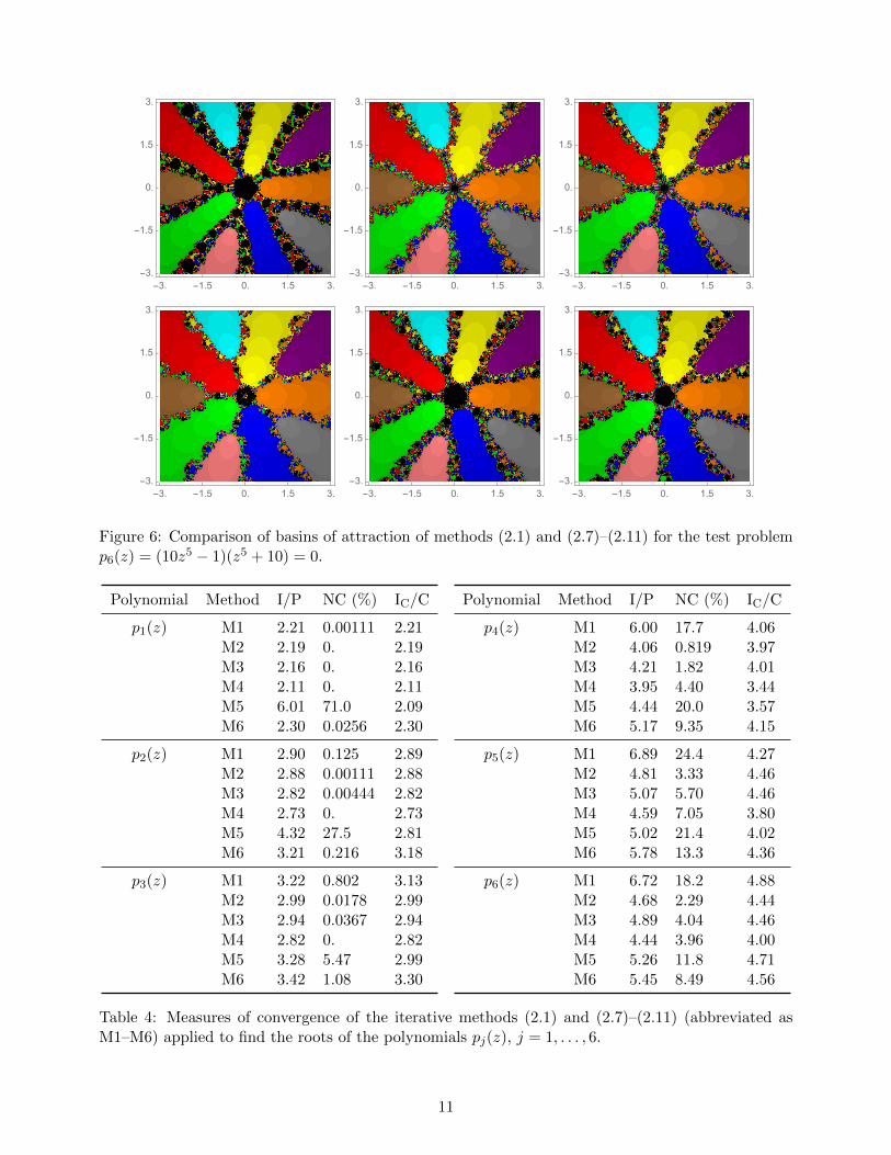
The six methods (2.1) and (2.7)–(2.11) provide iterative rational maps Q when they are appliedto find roots of complex polynomials p. In particular, we are interested in the basins of attraction ofthe roots of the polynomials where the basin of attraction of a root z∗ is the complex set {z0 ∈ C :orb(z0) → z∗}. It is well known that the basins of attraction of the different roots lie in the Fatouset F (Q). The Julia set J(Q) is, in general, a fractal and the rational map Q is unstable there.

For the dynamical and graphical point of view, we take a 600× 600 grid of the square [−3, 3]×[−3, 3] ⊂ C and assign a color to each point z0 ∈ D according to the simple root to which thecorresponding orbit of the iterative method starting from z0 converges, and we mark the point asblack if the orbit does not converge to a root in the sense that after at most 15 iterations it has adistance to any of the roots which is larger than 10−3. We have used only 15 iterations because weare using methods of convergence order eight which, if they converge, do this very fast. The basinsof attraction are distinguished by their color.

Test polynomials Roots

p1(z) = z2 − 1 1, −1

p2(z) = z3 − z 0, 1, −1

p3(z) = z(z2 + 1)(z2 + 4) 0, 2i, −2i, i, −ip4(z) = (z4 − 1)(z2 + 2i) 1, i, −1, −i, −1 + i, 1− ip5(z) = z7 − 1 e2kπi/7, k = 0, . . . , 6

p6(z) = (10z5 − 1)(z5 + 10)(

110

)1/5e2kπi/5, (−10)1/5e2kπi/5, k = 0, . . . , 4

Table 3: Test polynomials p1(z), . . . , p6(z) and their roots.

Different colors are used for different roots. In the basins of attraction, the number of iterationsneeded to achieve the root is shown by the brightness. Brighter color means less iteration steps. Notethat black color denotes lack of convergence to any of the roots. This happens, in particular, whenthe method converges to a fixed point that is not a root or if it ends in a periodic cycle or at infinity.Actually and although we have not done it in this paper, infinity can be considered an ordinary pointif we consider the Riemann sphere instead of the complex plane. In this case, we can assign a new“ordinary color” for the basin of attraction of infinity. Details for this idea can be found in [12].

Basins of attraction for the six methods (2.1) and (2.7)–(2.11) for the six test problems pi(z) = 0,i = 1, . . . , 6, are illustrated in Figures 1–6 from left to right and from top to bottom.

From the pictures, we can easily judge the behavior and suitability of any method depending onthe circumstances. If we choose an initial point z0 in a zone where different basins of attraction toucheach other, it is impossible to predict which root is going to be reached by the iterative method that

7

-3. -1.5 0. 1.5 3.

3.

1.5

0.

-1.5

-3.-3. -1.5 0. 1.5 3.

3.

1.5

0.

-1.5

-3.-3. -1.5 0. 1.5 3.

3.

1.5

0.

-1.5

-3.

-3. -1.5 0. 1.5 3.

3.

1.5

0.

-1.5

-3.-3. -1.5 0. 1.5 3.

3.

1.5

0.

-1.5

-3.-3. -1.5 0. 1.5 3.

3.

1.5

0.

-1.5

-3.

Figure 1: Comparison of basins of attraction of methods (2.1) and (2.7)–(2.11) for the test problemp1(z) = z2 − 1 = 0.

-3. -1.5 0. 1.5 3.

3.

1.5

0.

-1.5

-3.-3. -1.5 0. 1.5 3.

3.

1.5

0.

-1.5

-3.-3. -1.5 0. 1.5 3.

3.

1.5

0.

-1.5

-3.

-3. -1.5 0. 1.5 3.

3.

1.5

0.

-1.5

-3.-3. -1.5 0. 1.5 3.

3.

1.5

0.

-1.5

-3.-3. -1.5 0. 1.5 3.

3.

1.5

0.

-1.5

-3.

Figure 2: Comparison of basins of attraction of methods (2.1) and (2.7)–(2.11) for the test problemp2(z) = z3 − z = 0.

8

-3. -1.5 0. 1.5 3.

3.

1.5

0.

-1.5

-3.-3. -1.5 0. 1.5 3.

3.

1.5

0.

-1.5

-3.-3. -1.5 0. 1.5 3.

3.

1.5

0.

-1.5

-3.

-3. -1.5 0. 1.5 3.

3.

1.5

0.

-1.5

-3.-3. -1.5 0. 1.5 3.

3.

1.5

0.

-1.5

-3.-3. -1.5 0. 1.5 3.

3.

1.5

0.

-1.5

-3.

Figure 3: Comparison of basins of attraction of methods (2.1) and (2.7)–(2.11) for the test problemp3(z) = z(z2 + 1)(z2 + 4) = 0.

-3. -1.5 0. 1.5 3.

3.

1.5

0.

-1.5

-3.-3. -1.5 0. 1.5 3.

3.

1.5

0.

-1.5

-3.-3. -1.5 0. 1.5 3.

3.

1.5

0.

-1.5

-3.

-3. -1.5 0. 1.5 3.

3.

1.5

0.

-1.5

-3.-3. -1.5 0. 1.5 3.

3.

1.5

0.

-1.5

-3.-3. -1.5 0. 1.5 3.

3.

1.5

0.

-1.5

-3.

Figure 4: Comparison of basins of attraction of methods (2.1) and (2.7)–(2.11) for the test problemp4(z) = (z4 − 1)(z2 + 2i) = 0.

9

-3. -1.5 0. 1.5 3.

3.

1.5

0.

-1.5

-3.-3. -1.5 0. 1.5 3.

3.

1.5

0.

-1.5

-3.-3. -1.5 0. 1.5 3.

3.

1.5

0.

-1.5

-3.

-3. -1.5 0. 1.5 3.

3.

1.5

0.

-1.5

-3.-3. -1.5 0. 1.5 3.

3.

1.5

0.

-1.5

-3.-3. -1.5 0. 1.5 3.

3.

1.5

0.

-1.5

-3.

Figure 5: Comparison of basins of attraction of methods (2.1) and (2.7)–(2.11) for the test problemp5(z) = z7 − 1 = 0.

starts in z0. Hence, z0 is not a good choice. Both the black zones and the zones with a lot of colorsare not suitable for choosing the initial guess z0 if precise root should be reached. Although the mostattractive pictures appear when we have very intricate frontiers between basins of attraction, theycorrespond to the cases where the dynamic behavior of the method is more unpredictable and themethod is more demanding with respect to choice of the initial point.

Finally, we have included in Table 4 the results of some numerical experiments to measure thebehavior of the five iterative methods (2.1) and (2.7)–(2.11) in finding the roots of the test polynomialspj , j = 1, . . . , 6. To compute the data of this table, we have applied the six methods to the sixpolynomials, starting at an initial points z0 on a 600×600 grid in the rectangle [−3, 3]× [−3, 3] of thecomplex plane. The same way was used in Figures 1–6 to show the basins of attraction of the roots.In particular, we decide again that an initial point z0 has reached a root z∗ when its distance to z∗

is less than 10−3 (in this case z0 is in the basin of attraction of z∗) and we decide that the methodstarting in z0 diverges when no root is found in a maximum of 15 iterations of the method. We sayin this case that z0 is a “nonconvergent point”. In Table 4, we have abbreviated the methods (2.1)and (2.7)–(2.11) as M1–M6, respectively. The column I/P shows the mean of iterations per pointuntil the algorithm decides that a root has been reached or the point is declared nonconvergent. Thecolumn NC shows the percentage of nonconvergent points, indicated as black zones in the picturesof Figures 1–6. It is clear that the nonconvergent points have a great influence on the values of I/Psince these points contribute always with the maximum number of 15 allowed iterations. In contrast,“convergent points” are reached usually very fast due to the fact that we are dealing with methodsof order eight. To reduce the effect of nonconvergent points, we have included the column IC/Cwhich shows the mean number of iterations per convergent point. If we use either the columns I/Por the column IC/C to compare the performance of the iterative methods, we clearly obtain differentconclusions.

10

-3. -1.5 0. 1.5 3.

3.

1.5

0.

-1.5

-3.-3. -1.5 0. 1.5 3.

3.

1.5

0.

-1.5

-3.-3. -1.5 0. 1.5 3.

3.

1.5

0.

-1.5

-3.

-3. -1.5 0. 1.5 3.

3.

1.5

0.

-1.5

-3.-3. -1.5 0. 1.5 3.

3.

1.5

0.

-1.5

-3.-3. -1.5 0. 1.5 3.

3.

1.5

0.

-1.5

-3.

Figure 6: Comparison of basins of attraction of methods (2.1) and (2.7)–(2.11) for the test problemp6(z) = (10z5 − 1)(z5 + 10) = 0.

Polynomial Method I/P NC (%) IC/C

p1(z) M1 2.21 0.00111 2.21M2 2.19 0. 2.19M3 2.16 0. 2.16M4 2.11 0. 2.11M5 6.01 71.0 2.09M6 2.30 0.0256 2.30

p2(z) M1 2.90 0.125 2.89M2 2.88 0.00111 2.88M3 2.82 0.00444 2.82M4 2.73 0. 2.73M5 4.32 27.5 2.81M6 3.21 0.216 3.18

p3(z) M1 3.22 0.802 3.13M2 2.99 0.0178 2.99M3 2.94 0.0367 2.94M4 2.82 0. 2.82M5 3.28 5.47 2.99M6 3.42 1.08 3.30

Polynomial Method I/P NC (%) IC/C

p4(z) M1 6.00 17.7 4.06M2 4.06 0.819 3.97M3 4.21 1.82 4.01M4 3.95 4.40 3.44M5 4.44 20.0 3.57M6 5.17 9.35 4.15

p5(z) M1 6.89 24.4 4.27M2 4.81 3.33 4.46M3 5.07 5.70 4.46M4 4.59 7.05 3.80M5 5.02 21.4 4.02M6 5.78 13.3 4.36

p6(z) M1 6.72 18.2 4.88M2 4.68 2.29 4.44M3 4.89 4.04 4.46M4 4.44 3.96 4.00M5 5.26 11.8 4.71M6 5.45 8.49 4.56

Table 4: Measures of convergence of the iterative methods (2.1) and (2.7)–(2.11) (abbreviated asM1–M6) applied to find the roots of the polynomials pj(z), j = 1, . . . , 6.

11

5 Conclusion

We have introduced a new optimal three-point method without memory for approximating a simpleroot of a given nonlinear equation which use only four function evaluations each iteration and resultin a method of convergence order eight. Therefore, Kung and Traub’s conjecture is supported.Numerical examples and comparisons with some existing eighth-order methods are included andconfirm the theoretical results. The numerical experience suggests that the new method is a valuablealternative for solving these problems and finding simple roots. We used the basins of attraction forcomparing the iterative algorithms and we have included some tables with comparative results.

Acknowledgments. The research of the fourth author is supported by grant MTM2015-65888-C4-4 from DGI (Spanish Government).

References

[1] Amat, S., Busquier, S., Magrenan, A.A.: Reducing chaos and bifurcations in Newton-type methods,Abstr. Appl. Anal. 2013, Art. ID 726701, 10 pages (2013).

[2] Babajee, D.K.R., Cordero, A., Soleymani, F., Torregrosa, J.R.: On improved three-step schemes withhigh efficiency index and their dynamics, Numer. Algorithms 65, 153–169 (2014).

[3] Bi, W., Ren, H., Wu, Q.: Three-step iterative methods with eighth-order convergence for solving nonlinearequations, J. Comput. Appl. Math. 225, 105–112 (2009).

[4] Chicharro, F., Cordero, A., Gutierrez, J.M., Torregrosa, J.R.: Complex dynamics of derivative-freemethods for nonlinear equations, Appl. Math. Comput. 219, 7023–7035 (2013).

[5] Chun, C., Lee, M.Y.: A new optimal eighth-order family of iterative methods for the solution of nonlinearequations, Appl. Math. Comput. 223, 506–519 (2013).

[6] Cordero, A., Torregrosa, J.R.: Variants of Newton’s method using fifth-order quadrature formulas, Appl.Math. Comput. 190, 686–698 (2007).

[7] Ezquerro, J.A., Hernandez, M.A.: An improvement of the region of accessibility of Chebyshev’s methodfrom Newton’s method, Math. Comp. 78, 1613–1627 (2009).

[8] Ezquerro, J.A., Hernandez, M.A.: An optimization of Chebyshev’s method, J. Complexity 25, 343–361(2009).

[9] Ferrara, M., Sharifi, S., Salimi, M.: Computing multiple zeros by using a parameter in Newton–Secantmethod, SeMA Journal, accepted (2016).

[10] Grau-Sanchez, M., Noguera, M., Gutierrez, J.M.: On some computational orders of convergence, Appl.Math. Lett. 23(4), 472–478 (2010).

[11] Gutierrez, J.M., Magrenan, A.A., Varona, J.L.: The “Gauss-Seidelization” of iterative methods for solvingnonlinear equations in the complex plane, Appl. Math. Comput. 218, 2467–2479 (2011).

[12] Hernandez-Paricio, L.J., Maranon-Grandes, M., Rivas-Rodrıguez, M.T.: Plotting basins of end points ofrational maps with Sage, Tbil. Math. J. 5(2), 71–99 (2012).

[13] Jarratt, P.: Some fourth order multipoint iterative methods for solving equations, Math. Comp. 20,434–437 (1966).

[14] King, R.F.: A family of fourth order methods for nonlinear equations, SIAM J. Numer. Anal. 10, 876–879(1973).

12

[15] Kung, H.T., Traub, J.F.: Optimal order of one-point and multipoint iteration, J. Assoc. Comput. Mach.21, 634–651 (1974).

[16] Lotfi, T., Sharifi, S., Salimi, M., Siegmund, S.: A new class of three-point methods with optimal conver-gence order eight and its dynamics, Numer. Algorithms 68, 261–288 (2015).

[17] Neta, B.: On a family of multipoint methods for nonlinear equations, Internat. J. Comput. Math. 9,353–361 (1981).

[18] Neta, B., Chun, C., Scott, M.: Basins of attraction for optimal eighth order methods to find simple rootsof nonlinear equations, Appl. Math. Comput. 227, 567–592 (2014).

[19] Ostrowski, A.M.: Solution of Equations and Systems of Equations, 2nd ed., Academic Press, New York(1966).

[20] Petkovic, M.S., Neta, B., Petkovic, L.D., Dzunic, J.: Multipoint Methods for Solving Nonlinear Equations,Elsevier/Academic Press, Amsterdam (2013).

[21] Sharifi, S., Ferrara, M., Salimi, M., Siegmund, S.: New modification of Maheshwari method with optimaleighth order of convergence for solving nonlinear equations, preprint (2015).

[22] Sharifi, S., Siegmund, S., Salimi, M.: Solving nonlinear equations by a derivative-free form of the King’sfamily with memory, Calcolo, doi: 10.1007/s10092-015-0144-1 (2015).

[23] Sharifi, S., Salimi, M., Siegmund, S., Lotfi, T.: A new class of optimal four-point methods with conver-gence order 16 for solving nonlinear equations, Math. Comput. Simulation 119, 69–90 (2016).

[24] Sharma, J.R., Sharma, R.: A new family of modified Ostrowski’s methods with accelerated eighth orderconvergence, Numer. Algorithms 54, 445–458 (2010).

[25] Stewart, B.D.: Attractor Basins of Various Root-Finding Methods, M.S. thesis, Naval PostgraduateSchool, Monterey, CA (2001).

[26] Thukral, R., Petkovic, M.S.: A family of three-point methods of optimal order for solving nonlinearequations, J. Comput. Appl. Math. 233, 2278–2284 (2010).

[27] Traub, J.F.: Iterative Methods for the Solution of Equations, Prentice Hall, Englewood Cliffs, N.J. (1964).

[28] Varona, J.L.: Graphic and numerical comparison between iterative methods, Math. Intelligencer 24(1),37–46 (2002).

[29] Wang, X., Liu, L.: New eighth-order iterative methods for solving nonlinear equations, J. Comput. Appl.Math. 234, 1611–1620 (2010).

[30] Weerakoon, S., Fernando, T.G.I.: A variant of Newton’s method with accelerated third-order convergence,Appl. Math. Lett. 13(8), 87–93 (2000).

13