Meshing implicit algebraic surfaces: the

smooth case

L. Alberti? & G. Comte◦ & B. Mourrain?

? GALAAD, INRIA ◦ Lab. J. A. DieudonneBP 93 Parc Valrose06902 Sophia Antipolis 06034 Nice cedexFrance France

Abstract. In this paper, we present a new algorithm to meshsurfaces defined by an implicit equation, which is able to isolatethe singular points of the surface, to guaranty the topology in thesmooth part, while producing a number of triangles which is relatedto geometric invariants of the surface. We prove its termination andcorrectness and give complexity bounds, based on metric entropyanalysis. The method applies to surfaces defined by a polynomialequation or a spline equation. We use Bernstein bases to representthe function in a box and subdivide this representation accordingto a generalization of Descartes rule, until the problem in each boxboils down to the case where either the implicit object is isotopic toits linear approximation in the cell or the size of the cell is smallerthan a parameter ε. This ensures that the topology of the implicitsurface is caught within a precision ε. Experimentations on classicalexamples from the classification of singularities show the efficiencyof the approach.

§1. Introduction

Several methods have been developed over the last decades to visualizeor to mesh an implicit surface. We mention in particular the followingapproaches:

• ray tracing,

XXX 1xxx and xxx (eds.), pp. 1–4.

Copyright c© 200x by Nashboro Press, Brentwood, TN.

ISBN 0-9728482-x-x

All rights of reproduction in any form reserved.

2 L. Alberti & G. Comte & B. Mourrain

• marching cube,

• marching polygonizer,

• deformation methods,

• subdivision methods.

Used to detect the visibility of objects, “ray tracing” methods [16] computethe intersection between the ray from the eye of the observer and the firstobject of the scene, for each pixel of the image. The rendering is verygood, but the computing time is significant. It depends on the resolutionof the scene to be viewed, and can produce only images in 2 dimensions.Moreover, computation cannot (a priori) be re-used for other views. Othertechniques, such as particle sampling, also use clouds of points lying onthe surface, to visualize it. See for instance [2]. However, it only yields anapproximation of the surface [28] without the topological structure, norwith guaranty on the result.

The “marching cube” algorithm [19] developed in order to reconstructimages in 3 dimensions starting from medical data, is very much used forvisualization of level sets of functions. The principle of this algorithm issimple: the domain of interest is divided in several cells, generally boxes,of the same size. At the corners of each cell, the values of the function fare calculated and a triangular mesh is then deduced according to the signof the function at these corners. This triangulation may not capture thetopology of the surface, if it is not supported by additional calculation.Several triangulations are possible for the same combination of signs. Somepartial solutions exist to avoid some of these ambiguities [18]. The coveringof all the space of study increases the computing time considerably. Indeedthe boxes not cut by the surface are not useful. Despite its defects, the“marching cube” methods remains a reference for its simplicity and itseasiness of adaptation.

The marching polygonizer method brings a significant improvementto the marching cube method. The principal idea of this method is tocalculate only the “useful” cells, that is, those which cut the surface. Thealgorithm starts from a valid cube (or tetrahedron), and propagate towardthe connected cells, which cut the surface [5], [6], [14], [1]. Thus it isnecessary to start from a cell intersecting the surface. Again, for selfintersecting surfaces or surfaces with singularities, the result might beerroneous. The algorithm is rather effective, but it does not make itpossible to mesh any surface correctly, if this one has, for example, severalconnected components, without using external tools such as “topologicalskeleton ” [4].

Deformation methods exploit results from Morse theory, in order tocorrectly follow the transformation of the level-sets f(x) = t [1]. See also[7] for a connected approach, which applies for smooth surfaces. These

Meshing algebraic surfaces 3

methods assume implicitly that the function is a Morse function, ie. thecritical points that are traversed during the deformation are not degener-ate. This is not always the case nor is straightforward to check.

We describe here a new subdivision algorithm to mesh an implicitsurface, which is able to isolate the singular points of the surface, to guar-anty the topology in the smooth part, while producing a number of linearpieces, related to the Vitushkin variations of the surface. It applies tosurfaces defined by a polynomial equation or a B-spline equation. Ourmethod has similarities with the one presented in [22], but we go furtherby describing a new and guaranteed subdivision criterion. Moreover, weanalyze in detail the complexity of the subdivision algorithm in terms ofthe entropy of the surface, which yields a bound on the number of cellsproduced by the method in terms of geometric invariants of the surface.The termination and correctness of the algorithm are proved, in the caseof a smooth surface. Its extension for the treatment of singularities, usinga local conic structure theorem, is briefly mentioned, but the extendeddetails of this treatment are postponed to another paper.

Regarding the technical aspects, we use Bernstein bases to representthe function in a box and subdivide this representation according to ageneralization of Descartes’ rule, until the problem in each box boils downto the case where either the implicit object is proved to be homeomorphto the computed linear approximation in the cell or the size of the cell issmaller than ε. This ensures that the topology of the implicit surface iscaught within a precision ε, where ε is a tunable parameter. Experimen-tations on classical examples from the classification of singularities showthe efficiency of the approach.

§2. Algebraic ingredients

For any point p ∈ R3, and any set A ⊂ R3, dist(p, A) denotes the minimalEuclidean distance between p and points q ∈ A. We define distx(p, A)as the minimal Euclidean distance between p and a point q ∈ A withthe same (y, z)-coordinates, if it exists and +∞ otherwise. The distancesdisty(p, A), distz(p, A) are defined similarly.

2.1. Representation of polynomials

Let us recall that a univariate polynomial f(x) of degree d can berepresented in the Bernstein basis by:

f(x) =d∑

i=0

bi Bid(x),

where Bid(x) = (d

i )xi(1− x)d−i. The sequence b = [bi]i=0,...,d is called the

set of control coefficients on [0, 1]. The polynomials Bid form the Bernstein

4 L. Alberti & G. Comte & B. Mourrain

basis on [0, 1]. Similarly, we will say that a sequence b represents thepolynomial f on the interval [a, b] if:

f(x) =d∑

i=0

bi (di )

1(b− a)n

(x− a)i(b− x)d−i.

The polynomials

Bid(x; a, b) := (d

i )1

(b− a)n(x− a)i(b− x)d−i

form the Bernstein basis on [a, b]. Hereafter, we are going to consider thesequence of values b together with the corresponding interval [a, b]. A firstproperty of this representation is that the derivative f ′ of f , is representedby the control coefficients:

d∆b := d(bi+1 − bi)06i6d−1.

Another fundamental algorithm that we will use on such a representationis the de Casteljau algorithm [10]:

b0i = bi i = 0, . . . , d

bri = (1− t) br−1

i + t br−1i+1 (t) i = 0, . . . , d− r

It allows us to subdivide the representation of p into the two sub-represen-tations on the intervals [a, (1−t)a+tb] and [(1−t)a+tb, b]. For a completelist of methods on this representation, we refer for instance to [10].

By a direct extension to the multivariate case, any polynomial f(x, y, z)of degree d1 in x ,d2 in y, d3 in z, can be decomposed as:

f(x, y, z) =d1∑

i=0

d2∑j=0

d3∑k=0

bi,j,kBid1

(x; a1, b1) Bjd2

(y; a2, b2) Bkd3

(z; a3, b3),

where (Bid1

(x; a1, b1) Bjd2

(y; a2, b2) Bkd3

(z; a3, b3))0≤i≤d1,0≤j≤d2,0≤k≤d3is the

tensor product Bernstein basis on the domain D := [a1, b1] × [a2, b2] ×[a3, b3]. The polynomial f is represented in this basis by the third ordertensor of control coefficients b = (bi,j,k)0≤i≤d1,0≤j≤d2,0≤k≤d3 .

Hereafter, we will denote by a cell , the pair of the box [a1, b1]×[a2, b2]×[a3, b3] together with the control coefficients b, representing f . The size ofa cell will be max{|b1 − a1|, |b2 − a2|, |b3 − a3|}.

De Casteljau algorithm also applies in the x, y or z-direction. Be-cause of this tensor product representation, the control coefficients of thederivative ∂xf(x, y, z) are given by:

d (bi+1,j,k − bi,j,k)0≤i≤d1−1,0≤j≤d2,0≤k≤d3

Meshing algebraic surfaces 5

and similarly for the derivatives ∂yf , ∂zf .Notice that the univariate Bernstein representation also extends to a

so-called triangular Bernstein basis. This representation can also be usedin our approach, but we will concentrate on the tensor product one.

2.2. Univariate solver

The subdivision criterion that we are going to use, is based on Descar-tes’ rule for a univariate polynomial with control coefficients b in theBernstein basis. The number of sign changes of a sequence b, also calledthe sign variation of b, is denoted hereafter by V (b).

Proposition 1. [10], [26] The number of sign changes V (b) of the controlcoefficients b = [bi]i=0,...,d of a univariate polynomial on [0, 1] bounds itsnumber of real roots in [0, 1] and is equal to it modulo 2.

Thus, by this proposition,

• if V (b) = 0, the number of real roots in [0, 1] is 0;

• if V (b) = 1, the number of real roots in [0, 1] is 1.

This yields the following simple but efficient algorithm:

Algorithm 1.Input: A precision ε and a polynomial f represented in the Bernsteinbasis of an interval [b, a]: f = (b, [a, b]).

• Compute the number of sign changes V (b).

• If V (b) > 1 and |b − a| > ε, subdivide the representation into twosub-representations b−,b+, corresponding to the two halves of theinput interval and apply recursively the algorithm to them.

• If V (b) > 1 and |b − a| < ε, output the ε/2-root (a + b)/2 withmultiplicity V (b).

• If V (b) = 0, remove the interval [a, b].

• If V (b) = 1, the interval contains one root, that can be isolatedwithin the precision ε.

Output: list of subintervals of [a, b] containing exactly one real root of for of ε-roots with their multiplicities.

In the presence of a multiple root, the number of sign changes of a repre-sentation containing a multiple root is bigger than 2, and the algorithmsplits the box until its size is smaller than ε.

In order to analyze the behavior of the algorithm, we used a partialinverse of Descartes’ rule [23] (see also [21]), to show that if f(x) = 0 has

6 L. Alberti & G. Comte & B. Mourrain

only simple roots on [a, b], an upper bound of the number of recursionsteps of the algorithm 1 is

l = dlog2

(1 +

√3

2s

)e,

where s is the minimal distance between the complex roots of f .Notice that this localization algorithm extends naturally to B-splines,

which are piecewise polynomial functions [10].

§3. Toward a guaranteed method

The aim of this section is to describe the method, which allows usto build a mesh of the surface f(x, y, z) = 0 in a domain D = [a1, b1] ×[a2, b2] × [a3, b3] ⊂ R

3, having the same topology as the surface. Theset of points (x, y, z) in D such that f(x, y, z) = 0 will be denoted byS := Z(f) ∩ D. The set of singular points of S (where f = ∂xf = ∂yf =∂zf = 0) will be denoted by Ssing, the set of smooth (non-singular) pointsof S by Ssmooth.

3.1. Description of the algorithmThe general scheme of the meshing algorithm is as follows:

• Represent the polynomial f(x, y, z) in the Bernstein basis adaptedto the domain D = [a1, b1]× [a2, b2]× [a3, b3] as follows:

f(x, y, z) =d1∑

i=0

d2∑j=0

d3∑k=0

bi,j,k Bid1

(x) Bjd2

(y) Bkd3

(z),

• Subdivide the box into smaller boxes (using de Casteljau algorithm)until the topology in these boxes can be certified or the size of thebox is smaller than ε.

It leads to the following scheme:

Algorithm 2.L := [Cell(f,D)];while (L is not empty){C := first_cell_of(L);if(topology_guaranty(C) && size(C) < epsilon_smooth )insert C at the head in the list of solutions;

else if(not(topology_guaranty(C)) && size(C)< epsilon_sing)insert C at the head in the list of (unmeshed) solutions;

else {

Meshing algebraic surfaces 7

subdivide the cell C;insert the new generated cells at the tail of L;remove C from L;

}}

The two parameters involved here are:

• εsmooth which is the maximal size of the cells where the topology isguaranteed,

• εsing, which is the minimal size after which we consider that the cellcontains a singular point.

Hereafter, to simplify the analysis of the algorithm, we will take ε =εsmooth = εsing. In practice, it could be interesting to have εsmooth > εsing,in order to compute large boxes in the smooth part and small boxes aroundthe singularities. This explain why we consider these two parameters.

This subdivision scheme produces a sequence of boxes F , which size isdecreasing. It corresponds to the construction of an octree, level by level.An advantage of the octree data-structure is the fast localisation of pointsand of faces or edges shared by several cells [27].

The subdivision criterion that we are going to use, is based on aextension of Descartes’ rule for a polynomial with control coefficientsb = (bi,j,k)06i6d1,0 ≤ j ≤ d2, 0 ≤ k ≤ d3 in the Bernstein basis.

In order to test whether we have to split a cell, we check if the numberof sign changes in one of the directions x, y, z is 0 or 1 and that the signvariation of the control coefficients of the derivative in this direction is 0.More precisely, the sign variation of f in the x direction is the maximumfor all j, k with 0 ≤ j ≤ d2, 0 ≤ k ≤ d3, of the sign variations of thesequences bj,k = (bi,j,k)0≤i≤d1 .

The stopping criterion that we use is the following:

Definition 2. The cell C is x-regular (resp. y, z-regular) for f , if thesign variation of b in the x (resp. y, z) direction is 0 or 1 and if thecoefficients of the derivative in this direction have a constant sign.

A similar definition applies to control coefficients of polynomials in twovariables on two-dimensional boxes.

Lemma 1. Let (u, v, w) be any permutation of (x, y, z). Assume that a(u, v)-facets F of a cell is u-regular for f . Then the topology of the surfacef = 0 on the face F is uniquely determined by its intersection points(counted with multiplicity) with the edges of the face.

Proof. Since f = 0 has no singular point on F , the trace of f = 0 on Fis a set of arc segments (possibly of length 0) intersecting the edges of the

8 L. Alberti & G. Comte & B. Mourrain

face. They project along the u-direction on the other axis (say the v-axis)as a set of non-overlapping intervals. Consequently, the topology of f = 0on F , is the same as those of the set of segments connecting the pointsof S on the edges, sorted according to their v coordinates and taken bypairs. This proves that the topology of the surface f = 0 on the facets ofthe cell is determined by the its points on the edges. �

Proposition 3. Let (u, v, w) be any permutation of (x, y, z). Assume thatC is u-regular and that the topology of f = 0 on the two (v, w)-facets of Cis known. Then the topology of the surface f = 0 in the box C is uniquelydetermined by its intersection points (counted with multiplicity) with theedges of the box.

Proof. We can assume without loss of generality, that f is u-regularon F , for u = x or u = y or u = z. According to the previous lemma,the topology of f = 0 on all the facets of the cell C is determined. Asinside the cell C the surface S is the graph of a function in the u-direction,and as there are no singular points of f = 0 in C, S ∩ C is topologicallyhomeomorphic to a set of discs which are determined by the projection ofthe segments of the facets, on a (v, w)-plane along the u -direction. Thisconcludes the proof. �

These lemma and proposition imply that checking the regularity of fin the box B and on faces, and computing the points of the surface onthe edges of the box allows us to deduce the topology of the surface inthe box. To compute the mesh in a regular cell, we need to compute thepoints of S (counted with their multiplicity) on the edges of the boxes.This is performed by the univariate solver (see algorithm 1).

This criterion implies that in the valid cells, the derivative of f inone direction is of constant sign and on the two faces transversal to thisdirection, another derivative is of constant sign. This may be difficult toobtain, when a point of the surface where two derivatives vanish is on (ornear) the border of the cell. In order to avoid this situation, we weakenthe criterion and improve the subdivision in the following way:

• We check that a derivative of f in one of the directions x, y, z has aconstant sign in the cell C. If not, the cell is subdivided.

• For the two faces transversal to this direction, we apply the samealgorithm on the faces (in 2 dimensions), in order to get polygonsrepresenting the trace of f = 0 on these faces.

In such a case, the topology of the set S in the cell C is guaranteed: Itis the graph of a function, say in the direction u for which the derivativehas a constant sign. The polygons of f = 0 on all the faces define closed

Meshing algebraic surfaces 9

curves on the border of C. Applying proposition 3, we are able to computethe topology of f = 0 in C.

Notice that if precautions are not taken, the trace of f = 0 on theborder of C might be a singular curve. To avoid this situation, we simplyprecompute the critical points of S for the projection in the directions(x, y), (x, z), (y, z). These points are defined by the equations f = ∂xf =∂yf = 0, f = ∂xf = ∂zf = 0, f = ∂yf = ∂zf = 0. In the case of asmooth surface, after a generic change of coordinates (or simply a generictranslation) the number of such points is finite (it is bounded by 3 d(d−1)2

where d = deg(f), by Bezout’s theorem). We avoid these points when thecells are subdivided, by choosing adequately the position of subdivision(applying de Casteljau algorithm for a value of t in between critical values).In order to apply recursively the algorithm in dimension 2, we take theparameters εsmooth = εsing = ε.

These adaptations allow us to prove that for a smooth surface andε small enough, the algorithm stops with the correct topology. By thestructure of the algorithm, we are able to detect if ε is not small enough.

To prove termination and correctness, we need the following definitionand result on the approximation of a function by the control polygon. LetK2(f) = maxp∈D ‖H2(f)(p)‖ where H2(f)(p) is the Hessian of f at p. LetC be a cell of size ε.

Let si,j,k be the points of the regular subdivision associated with thecontrol coefficients ci,j,k of f on C. Then there exists γ2(d) = γ2(d1, d2, d3)depending of d1 = degx(f), d2 = degy(f), d3 = degz(f) such that

|f(si,j,k)− ci,j,k| < γ2(d)K2(f)ε2. (1)

See eg. [24], [25], [20] for a proof and more details on this result. Wedenote κ2(f) = γ2(d)K2(f).

First, we analyze the cells which are rejected by the algorithm. Wedenote Γf (r) = {p ∈ D, |f(p)| 6 r}.

Proposition 4. Let C be a cell of size ε, outside Γf (κ2(f)ε2). Then thecontrol coefficients of f on C are of constant sign.

Proof. As C is outside Γf (κ2(f)ε2), f does not vanish in C, so that ithas a constant sign. Assume, without loss of generality, that f > 0 so thatf > κ2(f)ε2 > 0 in C. Then by (1), we have

ci,j,k = f(si,j,k)− (f(si,j,k)− ci,j,k) > κ2(f)ε2 − κ2(f)ε2 = 0.

�In consequence, such a cell will not be kept by the algorithm.

Theorem 1. If the surface S defined by f(x, y, z) = 0 is smooth in D,then the algorithm 2 stops for εsmooth > εsing small enough, and output amesh homeomorphic to S.

10 L. Alberti & G. Comte & B. Mourrain

Proof. By equation (1), for ε := εsmooth small enough, the cells C whichare kept by the algorithm intersect Γf (κ2(f)ε2).

Let us denote by x0 a point of Γf (κ2(f)ε2) ∩ C. For any x ∈ C, wehave

|f(x)− f(x0)| ≤ κ1(f) ||x− x0||∞ ≤ κ1(f)ε

where κ1(f) = maxp∈D ||(∂xf(p), ∂yf(p), ∂zf(p))||1. As x0 ∈ Γf (κ2(f)ε2),we have

|f(x))| ≤ κ1(f)ε + κ2(f)ε2,

which implies that C ⊂ Γf (κ1(f)ε+κ2(f)ε2). As S is smooth, for ε smallenough, we have

Γf (κ1(f)ε + κ2(f)ε2)∩ Γ∂xf (κ2(∂xf)ε2) ∩ Γ∂yf (κ2(∂yf)ε2) ∩ Γ∂zf (κ2(∂zf)ε2) = ∅.

This implies, for ε small enough, for any cell C of size ε kept by thealgorithm and for all x ∈ C, either |∂xf(x)| > κ2(∂xf)ε2 or |∂yf(x)| >κ2(∂yf)ε2 or |∂zf(x)| > κ2(∂zf)ε2. By equation (1), either ∂x(f) or ∂y(f)or ∂z(f) has its Bernstein coefficients of the same sign in C. A similarproof applies for the trace of f on the transversal faces, since we haveavoided the critical sections, for which the trace of f on the face is singu-lar. Consequently, for εsmooth and εsing small enough the algorithm stopson cells, in which the topology of f is guaranteed. �

3.2. Complexity analysis

In this section, we analyze the behavior of the algorithm as the size ofthe cells goes to 0. Let A be a subset of the surface S in the domain D.

Definition 5. We denote by C(ε, A) the minimal union of cells of size6 ε in the octree, covering A. Let N(ε, A) be the number of cells involvedin C(ε, A).

In order to analyze the number of boxes N(ε, A), we connect it to thefollowing notion [11], [29]:

Definition 6. (ε-entropy) For any set A in R3, let E(ε, A) be the min-imum number of closed balls of radius ε, covering A.

We will first show that N(ε, A) is of the same order than the entropyE(ε, A) of A ⊂ R3:

Proposition 7. E(ε, A) 6 N(ε, A) 6 γ0E(ε, A) where γ0 = µ(4√

3)where µ(r) is the minimal number of balls of radius 1, covering a ballof radius r.

Meshing algebraic surfaces 11

Proof. Since a cell of size ε is covered by a ball of radius ε, and C(ε, A)covers A, we have E(ε, A) 6 N(ε, A).

Since the Hausdorff distance between A and C(ε, A) is at most thelength

√3 ε of the diagonal of the cube, we have (see [29])

E(2√

3ε, C(ε, A)) 6 E(√

3 ε, A).

On the other hand, N(ν,A) 6 E(ν2 , C(ν,A)) since a cell of size ν, cannot

be covered by a single ball of radius ν2 , so that we have:

N(ε, A) 6 E(ε

2, C(ε, A)) 6 µ(4

√3)E(2

√3 ε, C(ε, A))

since E( νλ , A) ≤ µ(λ)E(ν,A) for λ > 0, ν > 0. We deduce that

N(ε, A) 6 µ(4√

3)E(√

3 ε, A) 6 µ(4√

3)E(ε, A),

since E(√

3 ε, A) ≤ E(ε, A) �

Next we will use the relations between the ε-entropy and the Vitushkinvariations, defined as follows:

Definition 8. For any set S ⊂ R3, let V0(S) be the number of connectedcomponents of S, and

Vi(S) = c(i)∫

L∈G3−i

V0(S ∩ L) dL,

where Gk is the Grassmannian of affine spaces of dimension k in R3, dLis the canonical measure on G3−i, and c(i) = 1∫

L∈G3−i

V0([0, 1]i ∩ L) dL,

(so that Vi([0, 1]i) = 1 and c(3) = 1).

Our aim is now to relate the number of boxes produced by the algo-rithm to geometric invariants of the surface, such as the variations Vi(S):

Theorem 2. Suppose that the surface S ⊂ D defined f(x, y, z) = 0, issmooth in D. Then the number N of cells produced by the algorithm forε = εsmooth is bounded by

N 6 γ0

(V0(S) +

1εV1(S) +

1ε2

V2(S))

. (2)

where γ0 ∈ R>0 is a universal constant.

12 L. Alberti & G. Comte & B. Mourrain

Proof. We use the following property [15], [29]:

E(ε, S) 6

(V0(A) +

1εV1(S) +

1ε2

V2(S) +1ε3

V3(S))

,

and the property that V3(S) = 0 since S is of dimension 2.Now by proposition 7, we have

N(ε, S) 6 γ′0

(V0(S) +

1εV1(S) +

1ε2

V2(S))

.

By proposition 4, in every cell outside Γf (κ2(f)ε2), the Bernstein co-efficients of f have the same sign. Thus such a cell is not kept by thealgorithm. Consequently, we have

N ≤ N(ε, Γf (κ2(f)ε2)).

As S is smooth in D, the function x ∈ D 7→ dist(x,S)|f(x)| is well defined and

bounded by a constant κ1(f).Thus, for ε small enough

Γf (κ2(f)ε2)) ⊂ Sε = {x ∈ D; dist(x, S) < ε}

We deduce thatN ≤ N(ε, Sε) ≤ 27N(ε, S),

since by surrounding each of the cells covering S, by its 26 neighbors cellswe cover the points of Sε at distance ε from S. This proves inequality (2),with γ0 = 27γ′0. �Notice that we can link V1(S) to the curvature of S, since there exists auniversal constant c1 such that

V1(S) 6 c1

∫Ssmooth

|k1(p)|+ |k2(p)|dp,

where k1(p), k2(p) are the principal curvatures of S at p.Similarly, we have

V2(S) = Area(S).

See [29], [17] for more details.

3.3. SingularitiesIn our framework the treatment of singular points is a delicate task, al-

though certifying the topology of a tame set (ie. algebraic, semi-algebraic,subanalytic or more generally a set definable in some o-minimal structure)near one of its points is formally possible, since such a set has locallyaround each of its points a cone-like topology. In some small enough ball

Meshing algebraic surfaces 13

centered at the special point p, our set as the same topology as the coneof vertex p constructed on the intersection of the set and the boundary ofthe ball.

This is a consequence of the existence of Whitney stratifications forthese sets and of general properties of topological uniform finiteness. Letus be more precise.

Let p ∈ S be a singular point of S and let βp : S 3 q → ‖q−p‖∞ where‖ · ‖∞ is the infinity norm. Note that the set β−1

p (r) = {q ∈ S, βp(q) = r}is the intersection of S with the faces of a box centered at p and of size2r. This map βp is semi-algebraic, so that the following theorem applies:

Theorem 3. [12]; [13] There exists ε0 ∈ R>0 such that for each 0 < r ≤ε0, (β−1

p (ε0), β−1p ([0, ε0])), (β−1

p (r), β−1p ([0, r])) and (β−1

p (r)×{1}, β−1p (r)×

[0, 1]/ ≡) are homeomorphic, where ≡ is defined on β−1p (r) × [0, 1] by

(x, t) ≡ (y, s) ⇔ t = s = 0.

In other words, for a sufficiently small cell C centered at a singularpoint p of S, the topology of S in the cell β−1

p (r), r ≤ ε0 is the sameas those of the cone of vertex p, “lying” on the curve β−1

p (ε0) given bythe intersection of S with the facets of C. In order to compute a coherentmesh in such a case, we compute the star-triangulation whose vertex is asingular point of the surface in the cell, and which basis is the piecewise-linear approximation of the curve of intersection of the surface with theboundary of the box. We will describe this meshing method near singularpoints in a forthcoming paper.

§4. Experimentation

We present here some experimentations on surfaces related to the classi-fication of singularities [3]. The implementation is available in the libraryaxel (Algebraic Software-Components for gEometric modeLing)1. Thetable reports on the number of triangles, of cells including the singularone denote by nt (represented by boxes in the pictures) and the timing.The tests have been run on a Pentium IV 2.4 Ghz workstation. We con-sider a smooth case, a case with finitely many singular points, with aself intersection curve and with the singular points containing an isolatedcurve arc2. The parameters used for the subdivision are εsmooth = 2−5 |D|and εsing = 2−8 |D|. The pictures show the corresponding mesh. In orderto get a better rendering we could compute the normal at points on thesurface. This is direct from the implicit equation, but is not done in thefollowing visualization. Notice also that once the topology is certified, thetriangulation can be improved in the smooth boxes, according to geometriccriteria [9], [8].

1http://www-sop.inria.fr/galaad/software/axel2More examples can be found at http://www-sop.inria.fr/galaad/data/surface/

14 L. Alberti & G. Comte & B. Mourrain

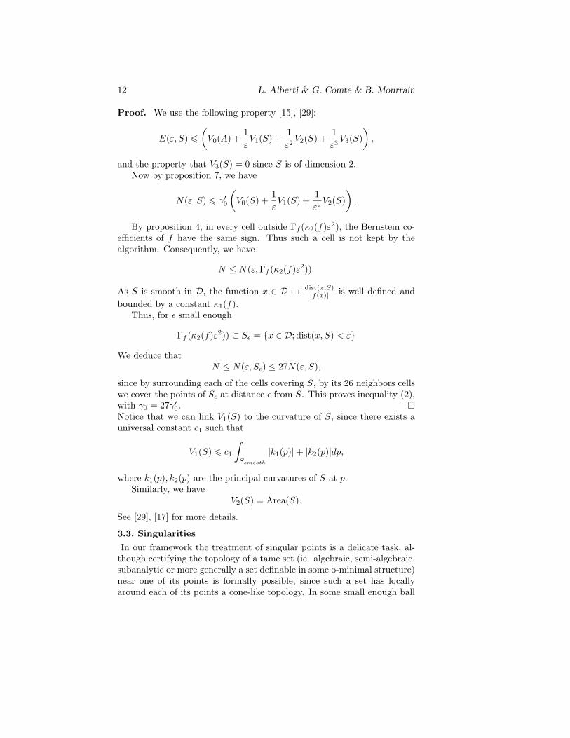
Equation:x4 − 5 x2 + y4 − 5 y2 + z4 − 5 z2

+11.8 = 0Nb of triangles: 8881Nb of cells: 4165Time (s): 1.53 s

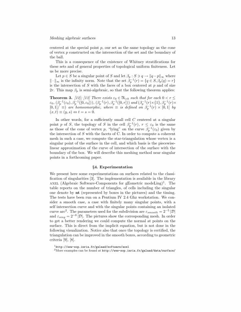
Equation:32 x8 − 64 x6 + 40 x4 − 8 x2 + 1 + 32 y8

−64 y6 + 40 y4 − 8 y2 + 32 z8 − 64 z6

+40 z4 − 8 z2 = 0Nb of triangles: 45680Nb of cells: 14555 + 594 ntTime (s): 8.13 s

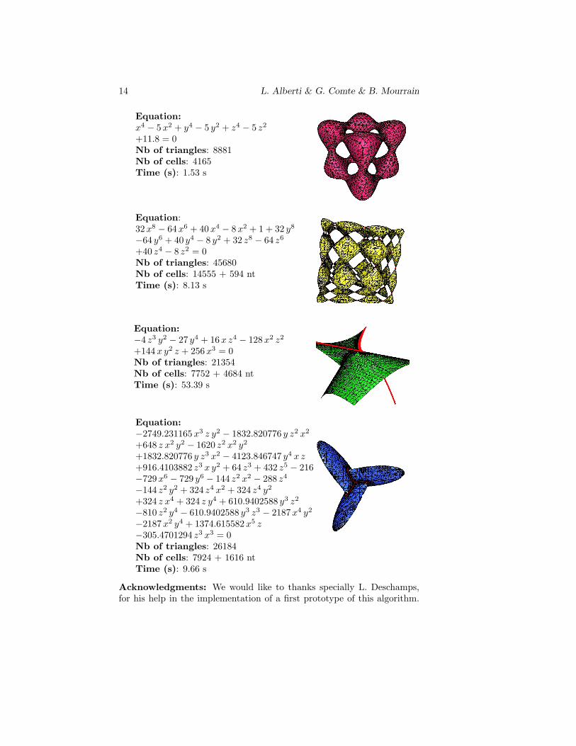
Equation:−4 z3 y2 − 27 y4 + 16 x z4 − 128 x2 z2

+144x y2 z + 256 x3 = 0Nb of triangles: 21354Nb of cells: 7752 + 4684 ntTime (s): 53.39 s

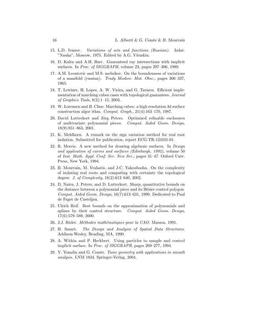
Equation:−2749.231165 x3 z y2 − 1832.820776 y z2 x2

+648 z x2 y2 − 1620 z2 x2 y2

+1832.820776 y z3 x2 − 4123.846747 y4 x z+916.4103882 z3 x y2 + 64 z3 + 432 z5 − 216 z6

−729 x6 − 729 y6 − 144 z2 x2 − 288 z4

−144 z2 y2 + 324 z4 x2 + 324 z4 y2

+324 z x4 + 324 z y4 + 610.9402588 y3 z2

−810 z2 y4 − 610.9402588 y3 z3 − 2187 x4 y2

−2187 x2 y4 + 1374.615582 x5 z−305.4701294 z3 x3 = 0Nb of triangles: 26184Nb of cells: 7924 + 1616 ntTime (s): 9.66 s

Acknowledgments: We would like to thanks specially L. Deschamps,for his help in the implementation of a first prototype of this algorithm.

Meshing algebraic surfaces 15

This work was partially supported by the european projects GAIA IST-2001-35512 and Aim@Shape FP6 IST NoE 506766.

§5. References

1. S Akkouche. and E. Galin. Adaptive implicit surface polygonizationusing marching triangles. Comput. Graph. Forum, 20(2):67–80, 2001.

2. Marc Alexa, Johannes Behr, Daniel Cohen-Or, Shachar Fleishman,David Levin, and Claudio T. Silva. Point set surfaces. In Proceedingsof the conference on Visualization ’01, pages 21–28. IEEE ComputerSociety, 2001.

3. V. Arnold, A. Varchenko, and S. M Gusein-Zade. Singularites desapplications differentiables. Edition Mir, Moscou, 1986.

4. J. F. Blinn. A generalization of algebraic surface drawing. ACM Trans-actions on graphics, 1(3):235–256, july 1982.

5. J. Bloomenthal. Polygonization of implicit surfaces. Computer-AidedGeometric Design, 5(4):341–355, 1988.

6. J. Bloomenthal. An implicit surface polygonizer. In Paul Heckbert,editor, Graphics Gems IV, pages 324–349. Academic Press, Boston,MA, 1994.

7. Jean-Daniel Boissonnat, David Cohen-Steiner, and Gert Vegter. Mesh-ing implicit surfaces with certified topology. Technical Report 4930,INRIA Sophia-Antipolis, 2003.

8. Jean-Daniel Boissonnat and Steve Oudot. An effective condition forsampling surfaces with guarantees. In Proc. Symp. on Geometry Pro-cessing, pages 9–18, 2004.

9. L. P. Chew. Guaranteed-quality mesh generation for curved surfaces. InProc. 9th Annu. ACM Sympos. Comput. Geom., pages 274–280, 1993.

10. G. Farin. Curves and surfaces for computer aided geometric design : apractical guide. Comp. science and sci. computing. Acad. Press, 1990.

11. H. Federer. Geometric measure theory, volume 153 of Grund. Math.Wiss. Springer-Verlag, 1969.

12. M. Goresky and R. MacPherson. Stratified Morse theory, volume 14 ofErgebnisse Math. Springer-Verlag, 1988.

13. R.M. Hardt. Semi-algebraic local-triviality in semi-algebraic mappings.Amer. J. Math., 102(2):291–302, 1980. (Mather Notes on topologicalstability, Harvard University, 1970).

14. E. Hartmann. A marching method for the triangulation of surfaces.Visual Computer, 14(3):95–108, 1998.

16 L. Alberti & G. Comte & B. Mourrain

15. L.D. Ivanov. Variations of sets and functions (Russian). Izdat.”Nauka”, Moscow, 1975. Edited by A.G. Vituskin.

16. D. Kalra and A.H. Barr. Guaranteed ray intersections with implicitsurfaces. In Proc. of SIGGRAPH, volume 23, pages 297–306, 1989.

17. A.M. Leontovic and M.S. melnikov. On the boundenness of variationsof a manifold (russian). Trudy Moskov. Mat. Obsc., pages 306–337,1965.

18. T. Lewiner, H. Lopes, A. W. Vieira, and G. Tavares. Efficient imple-mentation of marching cubes cases with topological guarantees. Journalof Graphics Tools, 8(2):1–15, 2003.

19. W. Lorensen and H. Cline. Marching cubes: a high resolution 3d surfaceconstruction algor ithm. Comput. Graph., 21(4):163–170, 1987.

20. David Lutterkort and Jorg Peters. Optimized refinable enclosuresof multivariate polynomial pieces. Comput. Aided Geom. Design,18(9):851–863, 2001.

21. K. Mehlhorn. A remark on the sign variation method for real rootisolation. Submitted for publication, report ECG-TR-123101-01.

22. R. Morris. A new method for drawing algebraic surfaces. In Designand application of curves and surfaces (Edinburgh, 1992), volume 50of Inst. Math. Appl. Conf. Ser. New Ser., pages 31–47. Oxford Univ.Press, New York, 1994.

23. B. Mourrain, M. Vrahatis, and J.C. Yakoubsohn. On the complexityof isolating real roots and computing with certainty the topologicaldegree. J. of Complexity, 18(2):612–640, 2002.

24. D. Nairn, J. Peters, and D. Lutterkort. Sharp, quantitative bounds onthe distance between a polynomial piece and its Bezier control polygon.Comput. Aided Geom. Design, 16(7):613–631, 1999. Dedicated to Paulde Faget de Casteljau.

25. Ulrich Reif. Best bounds on the approximation of polynomials andsplines by their control structure. Comput. Aided Geom. Design,17(6):579–589, 2000.

26. J.J. Risler. Methodes mathematiques pour la CAO. Masson, 1991.

27. H. Samet. The Design and Analysis of Spatial Data Structures.Addison-Wesley, Reading, MA, 1990.

28. A. Witkin and P. Heckbert. Using particles to sample and controlimplicit surface. In Proc. of SIGGRAPH, pages 269–277, 1994.

29. Y. Yomdin and G. Comte. Tame geometry with applications in smoothanalysis. LNM 1834. Springer-Verlag, 2004.