Method of Estimating the Principal Characteristics of an ...

I N S T I T U T E F O R D E F E N S E A N A L Y S E S

August 2013

IDA Paper P-5032Log: H 13-000777

Method of Estimating the PrincipalCharacteristics of an Infantry Fighting Vehicle

from Basic Performance Requirements

David R. GillinghamPrashant R. Patel, Project Leader

INSTITUTE FOR DEFENSE ANALYSES4850 Mark Center Drive

Alexandria, Virginia 22311-1882

Approved for public release;distribution is unlimited.

About this PublicationThis work was conducted by the Institute for Defense Analyses (IDA) under contract DASW01-04-C-0003, AU-7-3307.10, “Research on the Development and Application of Tools to Assist the OSD Office of Systems Engineering,” for the Director, Systems Engineering. The views, opinions, and findings should not be construed as representing the official position of either the Department of Defense or the sponsoring organization.

AcknowledgmentsThank you to Paul M. Kodzwa, David A. Sparrow, and Jeremy A. Teichman for performing technical review of this document.

Copyright Notice© 2013 Institute for Defense Analyses4850 Mark Center Drive, Alexandria, Virginia 22311-1882 • (703) 845-2000.

I N S T I T U T E F O R D E F E N S E A N A L Y S E S

IDA Paper P-5032

Method of Estimating the PrincipalCharacteristics of an Infantry Fighting Vehicle

from Basic Performance Requirements

David R. GillinghamPrashant R. Patel, Project Leader

Executive Summary

An infantry fighting vehicle (IFV) can be described by a few major performance parameters, such as number of crew and passengers, the protection level, and weapons type. The remainder of the performance requirements, such as mobility, can be assumed to match similar vehicles already in operation or be treated as independent variables. Once these parameters are set, much of the vehicle characteristics can be derived from practical constraints. For example, there is not much latitude in choosing spaces designed to accommodate seated persons. Also, the overall dimensions of the vehicle are constrained by transportability considerations. This leads to a relatively simple method for a notional design in which the protected cabin containing the crew, passengers, and auxiliary automotive and mission-related equipment that must be protected can be scaled according to the performance parameters. Once the protected volume is known, the weight of the armor can be determined by the surface areas to be protected and the threat level. The remaining propulsion and suspension systems can be also be scaled according to a combination of desired performance and algebraic relationships that relate to the vehicle’s overall vehicle weight. This design logic allows one to quickly determine all of the major characteristics of the IFV, such as size, weight, and the required engine power.

iii

Table of Contents

1. Introduction .................................................................................................................1 2. Volume of Interior Protected Space ............................................................................5

A. Cabin Dimensions Based on Crew and Passengers .............................................5 B. Additional Cabin Dimensions to Accommodate Equipment ............................12

3. Engine Sizing Considerations ....................................................................................17 4. Fuel Efficiency and Range ........................................................................................19 5. Weight of Power Plant and Drivetrain Components .................................................25 6. Volume of Drivetrain Components ...........................................................................31 7. Volume and Weight Allocations for Power Plant, Drivetrain, and Fuel ...................33 8. Weight of Turret ........................................................................................................35 9. Weight of Suspension Components ...........................................................................37 10. Determination of Gross Vehicle Weight and Size ....................................................43 11. Summary ....................................................................................................................49 Appendix A. Sensitivity Study ....................................................................................... A-1 Appendix B. Derivation of Cooling Fan Power vs. Engine Output Scaling....................B-1 Appendix C. Analysis of Engine Weight Scaling with Power Rating .............................C-1 Appendix D. Derivation of Scaling Law for the Minimum Metallic Armor Thickness

to Defeat Armor-Piercing Ammunition .................................................................. D-1 Illustrations ...................................................................................................................... E-1 References ........................................................................................................................ F-1 Abbreviations .................................................................................................................. G-1

v

1. Introduction

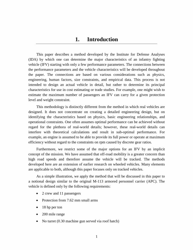
This paper describes a method developed by the Institute for Defense Analyses (IDA) by which one can determine the major characteristics of an infantry fighting vehicle (IFV) starting with only a few performance parameters. The connections between the performance parameters and the vehicle characteristics will be developed throughout the paper. The connections are based on various considerations such as physics, engineering, human factors, size constraints, and empirical data. This process is not intended to design an actual vehicle in detail, but rather to determine its principal characteristics for use in cost estimating or trade studies. For example, one might wish to estimate the maximum number of passengers an IFV can carry for a given protection level and weight constraint.

This methodology is distinctly different from the method in which real vehicles are designed. It does not concentrate on creating a detailed engineering design, but on identifying the characteristics based on physics, basic engineering relationships, and operational constraints. One often assumes optimal performance can be achieved without regard for the plethora of real-world details; however, these real-world details can interfere with theoretical calculations and result in sub-optimal performance. For example, an engine is assumed to be able to provide its full power or operate at maximum efficiency without regard to the constraints on rpm caused by discrete gear ratios.

Furthermore, we restrict some of the major options for an IFV by an implicit concept of the mission. We have assumed that off-road mobility is a greater concern than high road speeds and therefore assume the vehicle will be tracked. The methods developed here are an extension of earlier research on wheeled vehicles. Many elements are applicable to both, although this paper focuses only on tracked vehicles.

As a simple illustration, we apply the method that will be discussed in this paper to a notional design similar to the original M-113 armored personnel carrier (APC). The vehicle is defined only by the following requirements:

• 2 crew and 11 passengers

• Protection from 7.62 mm small arms

• 18 hp per ton

• 200 mile range

• No turret (0.30 machine gun served via roof hatch)

1

Table 1 compares the results to the actual M-113 APC.

Table 1. IFV Analysis Compared to M-113

Parameter Model Actual

Overall width (in) 78 72 Overall height (in) 104 106 Overall length (ft) 14.8 16.0 Engine rating (hp) 220 209 Fuel capacity (gal) 53 80 Gross vehicle weight (ton) 12.2 11.5

We also compare the model to the Bradley IFV (M2)-type design in Table 2 using

only the following requirements:


• Protection from 14.5 mm small arms

• 20 hp per ton

• 300 mile range

• Manned turret (2) with autocannon

Table 2. IFV Analysis Compared to M2

Parameter Model Actual

Overall width (in) 102 120 Overall height (in) 114 126 Overall length (ft) 13.8 21.1 Engine rating (hp) 435 500 Fuel capacity (gal) 145 175 Gross vehicle weight (ton) 22.1 25.1

As Table 1 and Table 2 show, this demonstration is successful, although we note

that this is not a validation in the usual sense. The designs that result from the model differ in many regards from the actual vehicles. Most notably, they have flat sides and use the same armor everywhere, whereas the actual vehicles have multiple surfaces and armor recipes even along the same side. A true comparison would require an actual vehicle made to the same simplistic design or would require that the model be so detailed as to lose almost all of its value for decision-making purposes. In fact, it is the simplicity of the model—free from detail—that makes it useful, especially in cases where no actual design exists, which is precisely where validation cannot be accomplished. Traditionally,

2

validation of a model can only be accomplished through use of the model to interpolate to cases that lie within the bounds of historical designs. The “validation” of this model comes from its individual parts, through either comparison with existing data or reliance on physics, which can be verified by the scientific community.

3

2. Volume of Interior Protected Space

We begin this process by determining the size of the most basic element of the vehicle, the protected volume that encloses the crew, passengers, and automotive and mission-related equipment. The basic structure and armor must enclose a space that contains the drive train (including electrical power generation), fuel storage, mission essential payload, integral auxiliary equipment, and people and their associated equipment. The turret is considered separately. We now proceed to establish some rules of thumb for estimating the size of this protected volume.

A. Cabin Dimensions Based on Crew and Passengers The most important items, of course, are the people. Human factors will dictate the

basic dimensions of a seated person. Each seated person requires a space 71 cm (28") wide, 132 cm (52") tall and 91 cm (36") long.1 That equates to about 0.85 m3 (30 ft3) per person. Persons who need to be able to move, such as the driver and crew, require a larger space, 91 x 132 x 91 cm, for a total volume of 1.10 m3 (39 ft3). In practice, volumes smaller than this are often used. The minimum possible dimensions are limited by anthropometric statistics, often for the 95th percentile male. From Figure 1, we see that the minimum width (shoulder room) is 56 cm, limited by the bideltoid width. The minimum length (leg room), assuming the knee is at 90 degrees, is 67 cm, limited by the buttock-knee length; however, leg room and head room can be traded off somewhat, so this need not be a definitive minimum. For example, one can imagine different sitting positions, from fully reclined to standing up. In this study, we will assume passengers are seated at a nearly 90-degree knee angle, so 67 cm will be the minimum leg room requirement.

The overall seated height is not directly measured, but can be approximated from the combination of knee height and sitting height, which together would be 156 cm for the 95th percentile male (Figure 1). Taking off about 10 percent for the distance between the seated knee height and the bottom of the buttocks, we estimate the overall seated height at 142 cm. If we combine the minimum width and length dimensions for the seated 95th percentile male, we get a volume of 0.5 m3. Therefore, the range of volumes per passenger range from the anthropometric minimum of 0.5 m3 to the human factors recommended value of 0.85 m3.

1 MIL-STD-1472G, Department of Defense Design Criteria Standard: Human Engineering (11 Jan 2012), Section 5.6.

5

Figure 1. Dimensions of the 95th Percentile Male

We check these dimensions against the volume allocations for some selected United

States (US) vehicles shown in Table 3 and Figure 2 through Figure 4. Some observations are that head room and shoulder room are almost always near the anthropometric minimum, while leg room is generally closer to the human factors recommendation. The use of the middle row jump seat in the M-113 seems to be the exception and results in sardine-like packing of the personnel, which is probably not an exemplary design, for various reasons. Most importantly in more modern designs, great consideration has been given to keeping the passenger’s feet off the cabin floor to prevent injuries during movement of the floor caused by mine detonation beneath the vehicle. The same would apply to blast-mitigating seats that require additional vertical room to reduce acceleration.

6

Table 3. Human Factors in Select Military Vehicles

Vehicle Height (cm) Shoulder (cm) Leg (cm) Volume (m3)

M-113 142 57 63 0.51 w/o jump seat 142 57 94 0.74 M1126 142 55 83 0.64 M2 142 62 96 0.85 ACT3010 152 59 86 0.77

There is some latitude in the actual arrangement of personnel inside the cabin, but

again, the overall volume requirement is more or less set. We start with a notional design and will show that there is an optimal configuration subject to some assumptions about constraints such as overall height and width. We begin by allocating 183 cm (72") to the cabin width as a starting bid. This would allow two operators to sit side-by-side or face-to-face. Using the human factors recommendations, passengers would be placed in two rows sitting face-to-face.

In addition to the width of the cabin, the overall vehicle width will include two tracks and exterior armor for the tracks. The tracks must lie outside of the cabin because they are typically about 1 m tall and if the cabin were located above that, the vehicle would be too tall. The track will depend on the weight class of the vehicle. The most limiting case is for vehicles up to 75 tons, in which the total width of the tracks would typically be about 122 cm (48"). Combined with our starting bid for cabin width, this already makes the total width of the vehicle about 305–318 cm (120–125"). Although one can make some trades in this area which can affect the trafficability (especially in urban environments), we consider 310 cm to be the maximum practical width for both road mobility and transportability,2 and treat this as a constraint.

As we shall see later in a sensitivity study provided as Appendix A, cabin width has a strong effect on the overall vehicle weight, with a sensitivity gain of -0.30 in a representative calculation. Sensitivity gain is defined as the fractional change in the overall vehicle weight relative to the fractional (small) change in a given parameter. In this case, for example, if we change the cabin width by +10 percent, the overall vehicle weight would change by -3 percent. Note the sign of the change: this means the weight goes down as the cabin is made wider. The reason for this is that the side protection is a leading factor in the overall vehicle weight for our representative calculation. The protected volume is fixed by the number of passengers and amount of interior equipment. When the cabin is made wider, the change in length reduces the area of the sides and therefore the weight of the side armor. The magnitude and sign of the sensitivity gain is

2 See MIL-STD-1366E, Department of Defense: Interface Standard for Transportability Criteria (31 Oct 2006), Sections 5.1-5.3; for example, NATO Envelope M.

7

specific to the application. We only argue that in the case of an IFV this calculation is representative, especially with regard to the sign of the change in weight.

Given this dependence, if we wish to keep the overall vehicle weight to a minimum (an admitted assumption about priorities), this leads to the conclusion that cabin width should be maximized consistent with keeping the overall vehicle width less than about 3.1 m (120"), meaning that one should use 182 cm (72") for the cabin width. One may choose not to constrain overall weight; however, almost every category of performance, including cost, is adversely affected by weight, with the possible exception of overall resistance to mines.

The same kind of logic will apply to the cabin height. A taller cabin results in a shorter vehicle (recall that the total volume is fixed), which reduces the area of the top and bottom, while the area of the sides stays constant. However, there are also limits on the overall vehicle height for the same reasons that the width is constrained. We first set the minimum interior cabin height at 132 cm (52") tall in order to account for human factors as well as clearance above the head for blast-resistant design features like energy-absorbing seats. Taller is better in terms of overall weight; however, we must take overall dimensions of the vehicle into account with regard to constraints.

Mine-resistant designs typically feature V-hulls, which is also our assumption here. If we just focus on the vertical impulse transferred from a mine blast via the ejecta, detonation gases, etc., we find it scales as cos2 𝜃, where θ is the angle of the “V” (𝜃 = 0 corresponds to a flat bottom). Performance in general is improved by increasing the angle of the “V”; however, there are many caveats to this statement.3 In any case, increasing the angle too much has a much more direct impact on vehicle performance, specifically with regard to ground clearance. If the level of the floor is raised to keep ground clearance constant, the center of gravity is also raised, which may cause lateral stability problems. This is a case in which we cannot derive the optimum “V” angle using only basic considerations; rather, it is a parameter that needs to be independently provided by subject matter experts. Lacking other information, we use an assumed value of 25 degrees.

For a 182 cm wide cabin, θ = 25o places the bottom of the “V” at least 43 cm (17") lower than the cabin floor. Allowing another 46 cm for ground clearance, we already have the top of the hull at 221 cm (87") above the ground. Allowing another 61 cm (24") for a turret, we are already at minimum of 282 cm (111") overall height, not accounting for the thickness of materials and for sensors and communications equipment, some of which may be removable for transport. We also know that heights over 310 cm are likely to be problematic for a variety of transport options, including deck height on Marine Prepositioning Ships; therefore, we take this as another constraint. Although weight is not

3 This discussion is beyond the scope of this paper.

8

as sensitive to the height as it is to width, cabin height should be maximized to minimize weight (sensitivity gain in a representative calculation is -0.06). Under these constraints, allowing at least 10 cm for the thickness of materials, the optimal height of the interior cabin should be no more than 152 cm (60") tall. Keeping with the human factors volume of 0.85 m3, but not necessarily the recommendation for elbow room, the shoulder width at the maximum cabin height comes out to be 61 cm which is consistent with previous designs.

We wish to keep as much flexibility for the designer with regard to the placement of the crew and passengers, particularly when there are not even pairs or they are placed around other equipment. For this reason, our design logic is as follows: fix the cabin dimensions based on transportability constraints, and then allocate length to the cabin based on volume vs. actual placement. This tends to average out the details of placement and also keeps the calculation generic, without requiring any detail. This will undoubtedly lead to some disagreement between the model and actual designs, but this is acceptable because we are not trying to design an actual vehicle; rather, we are trying to rough out the principal characteristics based on desired performance.

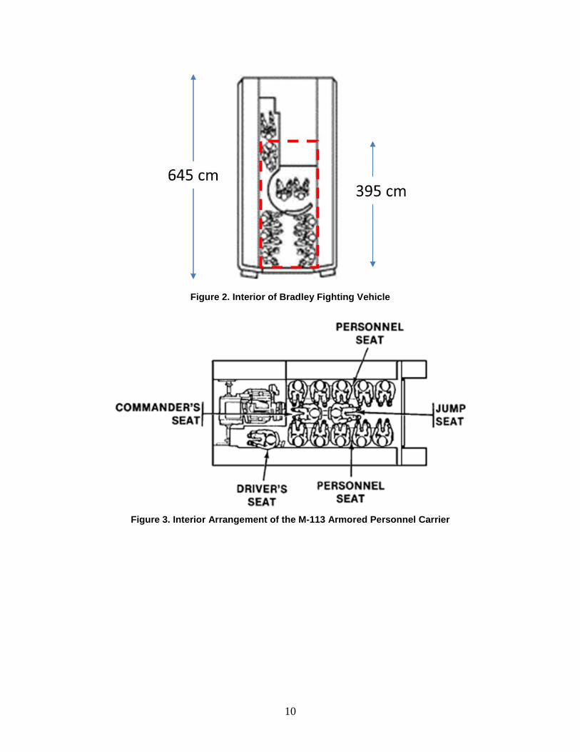
As an example of our allowance for personnel based on volume, consider the M1126. Based on the dimensions of the vehicle, we estimate the interior cabin has a cross-section of 2.4 m2. Looking at the arrangement in Figure 2, using four crew and six passengers, the model based on overall volume predicts that the interior volume should be (4 x 1.1) + (6 x 0.85) = 9.5 m3. The length should be 9.5/2.4 = 395 cm long. The interior length and width from this calculation is shown as a dashed red box. By comparison to the actual seating arrangement, one can see that the agreement of the model and actuality is relatively reasonable, using some imagination to move the driver alongside the crew in front of the turret. Note that the turret does not affect the volume calculation, which will be discussed later. The M-113 has a much more compact arrangement (Figure 3), while the M1126 has a more traditional layout (Figure 4).

9

Figure 2. Interior of Bradley Fighting Vehicle

Figure 3. Interior Arrangement of the M-113 Armored Personnel Carrier

10

Figure 4. Seating Arrangement in M1126 Infantry Carrier Vehicle

The following summarizes conclusions regarding space for crew and passengers:

• Minimum dimensions are constrained by anthropometric factors.

• Maximum dimensions are constrained by transportability factors.

• For designs where side protection is paramount, width and height should be maximized consistent with transportability constraints.

• This leaves length as the only free variable, which should be minimized for various reasons, leading to the conclusions that passengers should be seated face-to-face across the cabin, similar to the M1126, and the space allocation for shoulder room minimized consistent with the anthropometric bideltoid width.

• Using a volume allocation along with the dimensional restrictions above provides a somewhat design-independent way to estimate the cabin length allocation for crew and operators.

The proposed method has the following known limitations:

• It cannot provide an actual design for crew and passenger seating.

• It omits limitations of space usage resulting from internal structures and equipment placements.

• It does not provide for detailed allocations for ingress/egress.

11

• It omits details (but not principles) of blast-resistant design implementation.

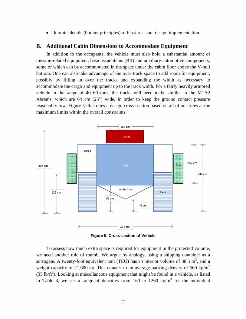
B. Additional Cabin Dimensions to Accommodate Equipment In addition to the occupants, the vehicle must also hold a substantial amount of

mission-related equipment, basic issue items (BII) and auxiliary automotive components, some of which can be accommodated in the space under the cabin floor above the V-hull bottom. One can also take advantage of the over-track space to add room for equipment, possibly by filling in over the tracks and expanding the width as necessary to accommodate the cargo and equipment up to the track width. For a fairly heavily armored vehicle in the range of 40–60 tons, the tracks will need to be similar to the M1A2 Abrams, which are 64 cm (25") wide, in order to keep the ground contact pressure reasonably low. Figure 5 illustrates a design cross-section based on all of our rules at the maximum limits within the overall constraints.

Figure 5. Cross-section of Vehicle

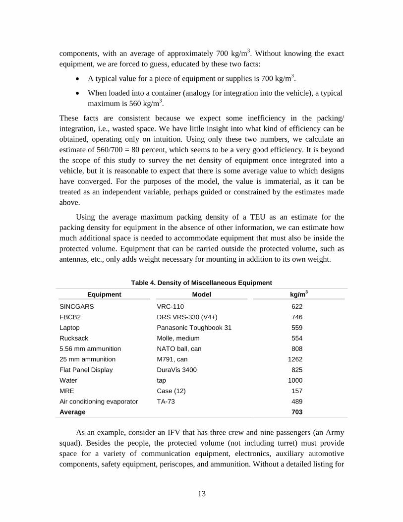
To assess how much extra space is required for equipment in the protected volume,

we need another rule of thumb. We argue by analogy, using a shipping container as a surrogate. A twenty-foot equivalent unit (TEU) has an interior volume of 38.5 m3, and a weight capacity of 21,600 kg. This equates to an average packing density of 560 kg/m3 (35 lb/ft3). Looking at miscellaneous equipment that might be found in a vehicle, as listed in Table 4, we see a range of densities from 160 to 1260 kg/m3 for the individual

12

components, with an average of approximately 700 kg/m3. Without knowing the exact equipment, we are forced to guess, educated by these two facts:

• A typical value for a piece of equipment or supplies is 700 kg/m3.

• When loaded into a container (analogy for integration into the vehicle), a typical maximum is 560 kg/m3.

These facts are consistent because we expect some inefficiency in the packing/ integration, i.e., wasted space. We have little insight into what kind of efficiency can be obtained, operating only on intuition. Using only these two numbers, we calculate an estimate of 560/700 = 80 percent, which seems to be a very good efficiency. It is beyond the scope of this study to survey the net density of equipment once integrated into a vehicle, but it is reasonable to expect that there is some average value to which designs have converged. For the purposes of the model, the value is immaterial, as it can be treated as an independent variable, perhaps guided or constrained by the estimates made above.

Using the average maximum packing density of a TEU as an estimate for the packing density for equipment in the absence of other information, we can estimate how much additional space is needed to accommodate equipment that must also be inside the protected volume. Equipment that can be carried outside the protected volume, such as antennas, etc., only adds weight necessary for mounting in addition to its own weight.

Table 4. Density of Miscellaneous Equipment

Equipment Model kg/m3

SINCGARS VRC-110 622 FBCB2 DRS VRS-330 (V4+) 746 Laptop Panasonic Toughbook 31 559 Rucksack Molle, medium 554 5.56 mm ammunition NATO ball, can 808 25 mm ammunition M791, can 1262 Flat Panel Display DuraVis 3400 825 Water tap 1000 MRE Case (12) 157 Air conditioning evaporator TA-73 489 Average 703

As an example, consider an IFV that has three crew and nine passengers (an Army

squad). Besides the people, the protected volume (not including turret) must provide space for a variety of communication equipment, electronics, auxiliary automotive components, safety equipment, periscopes, and ammunition. Without a detailed listing for

13

a specific application, we can only guess at how much is required. A sample listing is provided in Table 5.

Table 5. Notional Listing and Weight Estimates for Other Equipment in Protected Volume

Equipment Weight (kg)a

Auxiliary automotive (e.g., air conditioning) 680 Vehicle controls and instrumentation 230 Communications 45 Navigation and tracking 10 Electronic displays 20 Vision enhancement 10 Periscopes 20 Ammunition and missiles 800 Networks and mountings 90 Total 1915 a Estimates derived from various vendor datasheets for commercially-

available equipment.

The space for the crew and passengers requires:

3 crew @ 1.10 m3 each 9 passengers @ 0.85 m3 each Total 10.95 m3

The cabin cross-section is 1.52 x 1.83 = 2.78 m2; therefore, the necessary length is 10.95/2.78 = 3.94 m (12.9 ft).

The available space underneath the floor associated with a 25o V-hull is 3.94 x 0.912 tan(25o) = 1.5 m3. At the maximum packing density, that volume could hold 560 kg/m3 x 1.5 m3 = 860 kg of equipment. However, not all the under-floor space is really useable. Some space must be allocated for structural members to stiffen the v-hull against movement during mine blast. Therefore, we can only use some fraction of the available space. We estimate about half of the space is useable, so the packing density of the under-floor space is 280 kg/m3. In the example, 430 kg of equipment may be placed there, leaving 1484 kg to be placed elsewhere. It can be stored in the outboard storage wings or by lengthening the cabin. Outboard storage is preferred because it does not increase the overall dimensions of the vehicle, provided it does not extend beyond the width of the tracks.

The available space for the outboard storage, above the tracks but below the roof of the cabin, is approximately 100 cm tall by 60 cm deep. The exact shape is not particularly important, as the same volume can be achieved in various ways as needed to fit specific

14

equipment. The top will need the same level of protection as the cabin roof, but the bottom may be less armored, as the tracks will offer some protection from beneath. For design calculations, we can either assume a shape that will provide adequate scalable storage for the vehicle length or, alternatively, calculate the required volume (after constraining one dimension) for a more detailed equipment loadout. For our current purposes, we chose the latter because an IFV will need a fixed amount of equipment regardless of the number of passengers plus another amount that scales on a per-passenger basis (e.g., air conditioning).

First, let us make sure that the proposed outboard storage plan is adequate for the baseline vehicle with three crew and nine passengers. The maximum outboard storage is 100 cm tall and 60 cm deep, with a cross-sectional area of 1.2 m2, including both sides. Each additional passenger requires 0.85/2.78 = 0.30 m of cabin length. The associated outboard storage for each passenger would be 0.3 x 1.2 = 0.36 m3, which at maximum loading could hold 560 x 0.36 = 201 kg. Each crew position adds 1.1/2.78 x 1.2 x 560 = 257 kg. The total for three crew and nine passengers, therefore, is 3 x 257 + 9 x 201 = 2580 kg, which is more than enough for our sample loadout of 1484 kg of equipment. In this case, the outboard storage could be scaled down to minimize the weight penalty.

In order to provide both fixed and scaling (with length or passengers) values, we can write an expression for the weight of equipment to be accommodated in the protected volume (pv):

𝑊𝑝𝑣 = 𝑊𝑝𝑣0 + 𝑊𝑝𝑣′ 𝑁 ,

where N is the total number of passengers. The numbers are to be treated as independent parameters that can be adjusted when more specific detail on requirements in known. The recommended values for our baseline analysis are shown in Table 6. Note that for nine passengers, the total is 1920 kg, close to the total in Table 5.

Table 6. Recommended Baseline Values

Symbol Description Value

Wpv0 Weight of fixed equipment inside protected volume 1200 kg W’pv Weight per passenger of additional equipment inside

protected volume 80 kg per passenger

The design logic is to fix the cabin length as needed to accommodate the crew and

passengers, then adjust the width of the outboard storage (assuming the height is fixed) to accommodate the weight of auxiliary automotive and mission-related equipment that needs to be inside the protected volume. In the rare case where the outboard storage cannot accommodate all the equipment without extending over the tracks, it is possible to adjust the length as needed.

15

Based on considerations of the space required, we need not add space in the form of additional length for the turret, regardless of manning. Turrets can be configured either as a remote weapons station (unmanned), or operated by one or two persons (e.g., gunner and commander). In the case of one operator, we estimate that there must be at least a 91 cm (36") diameter inside, typically on-center, or 1.0 m3 (35 ft3) in a 152 cm (60") tall cabin. For two operators, about 2.0 m3 would be needed. The net effect is to require space roughly equivalent to one extra crew for the one-person turret, and two extra crew for the two-person turret, as can qualitatively be seen in Figure 2. Therefore, no additional space in the protected volume is necessary for turret operation other than that already allocated for the operators (crew).

We do, however, need additional length to accommodate the power plant, drivetrain, and fuel tanks. We can adopt the same basic shape and extend it, as long as we know the volume of the completely integrated power plant and drivetrain. In Section 5, we will see how this scales with rated power. We also need the fuel volume, which will be dependent on the desired maximum vehicle range via the fuel economy such that:

𝑉𝑓𝑢𝑒𝑙 = 𝑅𝑎𝑛𝑔𝑒 (𝑚𝑖𝑙𝑒𝑠)𝑚𝑝𝑔

,

where mpg is the miles per gallon rating of the vehicle. In the following sections, we establish that for fixed mobility and range performance requirements, the power requirement and fuel economy depend approximately linearly on the overall vehicle weight. Therefore, the volume for the drivetrain and fuel scale with vehicle weight. Because of this scaling, we need to algebraically solve for overall vehicle weight and simultaneously determine the volume required for the power plant, drivetrain, and fuel.

16

3. Engine Sizing Considerations

An engine must be the appropriate size to produce the desired performance. There are two main categories of performance: mobility and trafficability. Mobility refers to performance metrics such as acceleration, top speed, speed on trails or cross-country, maximum slope ascent, side slope stability, gap crossing, fording, and climbing over obstacles. Some of these metrics require specific engineering solutions, but many of them are directly affected by the engine power-to-weight ratio of the vehicle.4 Trafficability, usually applied to off-road conditions, is often specified as maximum percent of a given terrain that cannot be traversed (allowing for changes in direction to navigate around obstacles and impassable terrain). If we average over all types of terrain and locations, trafficability is most strongly correlated inversely with contact pressure, which is directly related to traction on-grade.5 Tracked vehicles have low contact pressure in general, and if we stick to a design with less than 134 kPa (20 psi), trafficability will be roughly invariant because it is not dominated by traction on-grade, but rather by impassable terrain—a fixed amount of obstacles for which there are no engineering solutions, e.g., a ravine. A less significant factor is the power to overcome small obstacles, which also depends on the weight of the vehicle, thus the power-to-weight ratio (W/kg).

All other mobility metrics, such as on-road maximum, maximum speed on-grade, and average cross-country speed, are limited by the power-to-weight ratio. For vehicles designed to operate off-road, a power-to-weight ratio of 16.4–20.5 W/kg (20–25 hp/ton) is sufficient to meet almost all of the normal mobility metrics. By comparison, the Abrams tank—a common standard used for brigade mobility requirements—has a power-to-weight ratio of 17.5 W/kg (at 70 tons gross vehicle weight (GVW)). Auxiliary loads such electronics and turret operation will reduce the fraction of power that can be used for mobility, so some allowance should be given for this depending on the mission details. In our case, we treat the power-to-weight ratio as a performance parameter that can be determined by examining mobility requirements, because there is such a close connection between the ratio and mobility. Once it is set, the engine size, volume, and weight can all be determined concurrently with setting the overall vehicle weight.

4 David R. Gillingham, “Mobility of Tactical Wheeled Vehicles and Design Rules of Thumb,” IDA Document NS D-3747 (Alexandria, VA: Institute for Defense Analyses, December 2009), 13–18.

5 Ibid., 29.

17

4. Fuel Efficiency and Range

Mileage depends on the energy content of fuel (per unit volume) u, the overall efficiency of the engine in converting the fuel into propulsion η, and the force opposing the motion of the vehicle F. Simply put, km per liter (kpl) is calculated by:

𝑘𝑝𝑙 = 𝜂𝑢𝐹

.

Note that these are metric units, but not common. The conversion to the more widely used miles per gallon (mpg) is 1 kpl = 2.35 mpg.

The force in the direction of motion acting on a vehicle at any one time is:

𝐹 = 𝑀𝑔[sin𝜑 + (𝜇 + 𝜇′𝑣) cos𝜑] + 12𝜌𝐶𝑑𝐴𝑓𝑣

2

where M is the mass of the vehicle, g = 9.8 m/s2 is the acceleration of gravity, µ is the velocity-independent motion resistance coefficient, µ’ is the velocity-dependent motion resistance coefficient, v is the velocity, ρ = 1.2 kg/m3 is the density of air, φ is the angle of the slope, Cd is the drag coefficient (two-dimensional), and Af is the frontal projected area. Note that slope is often referred to by grade = tanφ, sometimes in percent. For example, a 45o slope is the same as a 100 percent grade.

For mileage calculations, we ignore two terms: the force resulting from the grade and the drag term. The first term is quite significant, especially at any appreciable grade. However, the contributions from positive and negative grades tend to cancel each other on a closed course or as long as there is no net gain in altitude. Consider the work expended against gravity to climb and descend a grade illustrated in Figure 6. If we compute the portion of the work without any velocity-dependent terms, we get:

𝑊 = 𝑀𝑔[𝐿1 sin∅1 + 𝜇 𝐿1 cos𝜑1 − 𝐿2 sin∅2 + 𝜇 𝐿2 cos𝜑2].

The first and third terms cancel because:

𝐿1 sin∅1 = 𝐿2 sin∅2 = ℎ.

The other terms combine and simplify because:

𝜇 𝐿1 cos𝜑1 + 𝐿2 sin∅2 = 𝑥,

such that:

19

𝑊 = 𝑀𝑔 𝜇 𝑥.

In other words, the work is the same as if the vehicle had just travelled on a flat grade from start to finish.

Note: Assumes no net gain in altitude.

Figure 6. Geometry for Work Expended to Ascend and Descend Grade

With regard to the two velocity-dependent terms,6 one is associated with internal track friction, and the other comes from air drag. The drag term is ignored because it is only significant at high speeds. We can estimate the speed at which drag becomes an important factor. Let vd be the speed at which the drag term is equal to the speed-independent rolling resistance given by:

𝑣𝑑 = �2𝑀𝑔𝜇𝜌𝐶𝑑𝐴𝑓

.

If we estimate this speed using the following parameters typical of an IFV:

M = 45,000 kg,

µ = 0.03 (primary roads),

Cd = 1.0, and

Af = 6.5 m2,

6 𝐹 = 𝑀𝑔[sin𝜑 + (𝜇 + 𝜇′𝑣) cos𝜑] + 12𝜌𝐶𝑑𝐴𝑓𝑣

2

20

the calculation gives us a speed of 58 m/s (130 mph). Since the force is proportional to v2, the ratio of drag to speed-independent rolling resistance (v/vd)2 at 45 mph (a typical maximum speed of IFV requirements) is only 11 percent. The reason we can ignore this with relatively small effect on accuracy is that for this class of vehicle the mass is very high for its frontal area, as compared to unarmored vehicles where drag is a more important factor.

The velocity-dependent rolling resistance should not be neglected, especially for a tracked vehicle. A typical value7 for µ′ is 0.00054 s/m. At 15 m/s, the ratio of velocity-dependent rolling resistance to the velocity-independent rolling resistance on paved roads is about 27 percent. To accurately compute the contribution, we need only know the average velocity. To demonstrate this, we sum over a series of small segments, each with length xi and traversed at velocity vi. The overall work would be:

𝑊 = 𝑀𝑔(𝜇𝑥 + 𝜇′∑ 𝑥𝑖 𝑣𝑖𝑖 ),

where the total distance traveled is:

𝑥 = ∑ 𝑥𝑖 .𝑖

If we factor out x, we get:

𝑊 = 𝑀𝑔𝑥 �𝜇 + 𝜇′ 1𝑥∑ 𝑥𝑖 𝑣𝑖𝑖 �.

Making the substitution for the average velocity:

�̅� = 1𝑥∑ 𝑥𝑖 𝑣𝑖𝑖 ,

we get:

𝑊 = 𝑀𝑔 𝑥(𝜇 + 𝜇′�̅�).

So we see that the work only depends on the average velocity for a fixed value of rolling resistance in the case where we have a motion resistance that is linear in velocity.

For a given mission profile, over different types of terrain where the rolling resistance will vary, we can compute a weighted-average rolling resistance as:

�̅� = ∑ 𝑓𝑖(𝜇𝑖 + 𝜇′�̅�𝑖)𝑖 ,

where fi is the fraction of each road type (by distance), µi is the speed-independent rolling resistance coefficient, and �̅�𝑖 is the average speed for that road type. Note that the speed-

7 J. Wong, Theory of Ground Vehicles, 4th Ed. (Hoboken, John Wiley & Sons, 2008), 322.

21

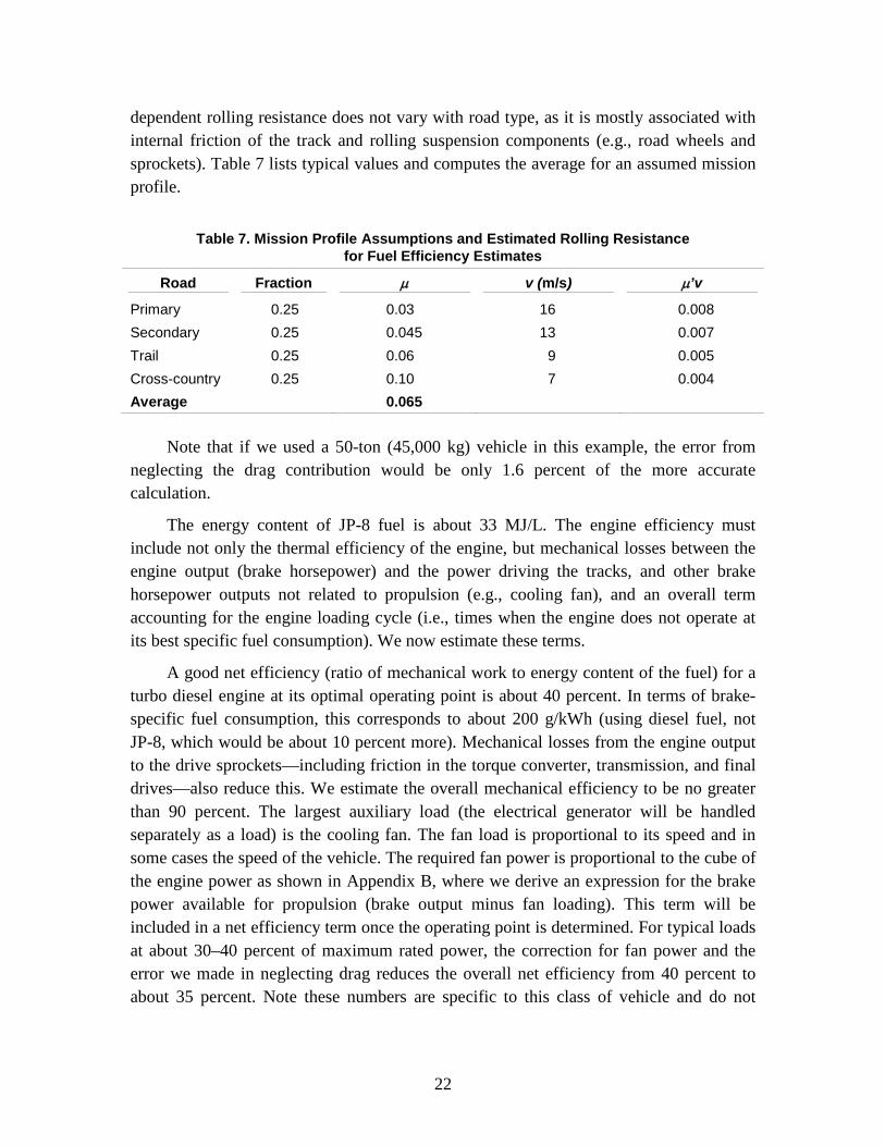
dependent rolling resistance does not vary with road type, as it is mostly associated with internal friction of the track and rolling suspension components (e.g., road wheels and sprockets). Table 7 lists typical values and computes the average for an assumed mission profile.

Table 7. Mission Profile Assumptions and Estimated Rolling Resistance

for Fuel Efficiency Estimates

Road Fraction µ v (m/s) µ’v

Primary 0.25 0.03 16 0.008 Secondary 0.25 0.045 13 0.007 Trail 0.25 0.06 9 0.005 Cross-country 0.25 0.10 7 0.004 Average 0.065

Note that if we used a 50-ton (45,000 kg) vehicle in this example, the error from

neglecting the drag contribution would be only 1.6 percent of the more accurate calculation.

The energy content of JP-8 fuel is about 33 MJ/L. The engine efficiency must include not only the thermal efficiency of the engine, but mechanical losses between the engine output (brake horsepower) and the power driving the tracks, and other brake horsepower outputs not related to propulsion (e.g., cooling fan), and an overall term accounting for the engine loading cycle (i.e., times when the engine does not operate at its best specific fuel consumption). We now estimate these terms.

A good net efficiency (ratio of mechanical work to energy content of the fuel) for a turbo diesel engine at its optimal operating point is about 40 percent. In terms of brake-specific fuel consumption, this corresponds to about 200 g/kWh (using diesel fuel, not JP-8, which would be about 10 percent more). Mechanical losses from the engine output to the drive sprockets—including friction in the torque converter, transmission, and final drives—also reduce this. We estimate the overall mechanical efficiency to be no greater than 90 percent. The largest auxiliary load (the electrical generator will be handled separately as a load) is the cooling fan. The fan load is proportional to its speed and in some cases the speed of the vehicle. The required fan power is proportional to the cube of the engine power as shown in Appendix B, where we derive an expression for the brake power available for propulsion (brake output minus fan loading). This term will be included in a net efficiency term once the operating point is determined. For typical loads at about 30–40 percent of maximum rated power, the correction for fan power and the error we made in neglecting drag reduces the overall net efficiency from 40 percent to about 35 percent. Note these numbers are specific to this class of vehicle and do not

22

generalize. For mileage calculations, we ignore the correction for fan power unless the mission profile involves a significant portion of operation at high power.

We estimate the mileage by equating the work done to the useable energy from fuel:

𝑀𝑔�̅�𝑥 = 𝜂𝑢𝑉𝑓𝑢𝑒𝑙 ,

where 𝑉𝑓𝑢𝑒𝑙 is the volume of fuel. The mileage is the ratio 𝑥/𝑉𝑓𝑢𝑒𝑙 which one can readily see is inversely proportional to the vehicle’s weight. If we extract the weight, we get a constant value that depends only on the mission profile and values of rolling resistance. To be fair, these depend somewhat on weight via ground contact pressure; however, we assume this is controlled by appropriate choice of track width such that ground contact pressure is relatively constant for all designs and therefore these values do not change much. Under these assumptions the ton miles-per-gallon can be computed by:

𝑡𝑜𝑛 ⋅ 𝑚𝑝𝑔 = 0.26 𝜂 𝑢[MJ/L]𝜇�

.

Using the following parameters,

η = 0.35 and

u = 33 MJ/L (JP-8),

along with our assumption of a mission profile and motion resistance values in Table 7, we get 𝑡𝑜𝑛 ∙ 𝑚𝑝𝑔 = 46. The volume for fuel for a given range becomes:

𝑔𝑎𝑙𝑙𝑜𝑛𝑠 𝑜𝑓 𝑓𝑢𝑒𝑙 = 𝑡𝑜𝑛∙𝑚𝑖𝑙𝑒𝑠 𝑡𝑜𝑛⋅𝑚𝑝𝑔

.

For example, a 50-ton vehicle for 300 miles is 15000 ton-miles. At 46 ton-mpg, that requires 1234 L (326 gal or 45 ft3) of JP-8 fuel. Note that this requires optimal operation of the engine, which is nearly impossible. Therefore, actual mileage may be substantially worse in reality, and 46 ton-mpg is only an upper bound for this mission profile. A more accurate calculation would require a level of detail that exceeds the general nature of the types of calculations and approximations in this document.

23

5. Weight of Power Plant and Drivetrain Components

In a previous analysis for tactical wheeled vehicles,8 a review of commercially available drivetrain components concluded that the mass and volume of the entire drivetrain system was linearly proportional to the engine’s rated power. This analysis was applicable up to 450 kW as this was the maximum engine rating expected for the vehicles of interest. We now revisit this analysis and consider whether it can be extended to tracked vehicles in the range of 450 to 1200 kW, the range of engine ratings appropriate for vehicles with gross vehicle weight ratings (GVWR) in the range of 30–75 tons. Appendix C outlines a number of arguments that support a linear model of engine weight to power rating. The value for the coefficient of proportionality as applied to tracked vehicles is discussed below.

For tracked military vehicles, space and weight are extremely limited, and considerable effort has been made to develop engines that are smaller and lighter for the same power. If we look only at combat vehicle applications over the last 40 years, we see a continuous evolution of engine design that has resulted in significant weight reduction. The most advanced military vehicle engine developer at this time is MTU Detroit Diesel. If we look at the current set of engines offered by MTU, listed in Table 8 and plotted in Figure 7, we see there are two sets of data: the established set of engines that line up more or less along a curve corresponding to 1.7 kW/kg, and the newest engine program, the 890-series, which line up along a curve corresponding to 1.0 kW/kg. The improvement in power density comes at the expense of engine stress. The brake mean effective pressure, �̅�𝑏, as discussed in Appendix C, has increased from the previous design generation of 10–20 bar, to a new average of 26 bar.

The product of �̅�𝑏 and mean piston speed vp, also discussed in Appendix C, which is directly related to the specific output (power per unit of piston area), is a good characterization of the overall engine stress. The peak pressure and wall temperature affect the mechanical and thermal stresses on the cylinder and piston. The inertial and friction loads on the piston and cylinder walls depend directly on the piston speed. Keeping this in mind, we note that the 890-series, which has the best power-to-weight ratio, has a product equal to 350 bar-m/s, whereas the average of previous designs for

8 Gillingham, IDA Document NS D-3747.

25

military vehicles is approximately 190 bar-m/s. This puts into perspective the level of advancement of these new designs.

Table 8. MTU Diesels for Heavy Defense Vehicles

Model Rating (kW) Mass (kg)

4R106 106 385 6R106 240 530 6V1992 430 920 8V1992 600 1135 MT 881 800 1400 MT 883 1200 1800 4R890a 370 450 5R890a 460 520 6V890a 550 610 10V890a 920 830

Source: All data taken from “Engines for heavy vehicles,” MTU.com, accessed 22 April 2003, http://www.mtu-online.com/mtu-northamerica/products/engine-program/diesel-engines-for-wheeled-and-tracked-armored-vehicles/engines-for-heavy-vehicles/. a Described as “projected development.”

Figure 7. Mass of High-speed, Turbo-boosted Diesel Engines Appropriate for Military

Vehicles from MTU as a Function of their Maximum Power Rating

The weight of the engine is only part of the drivetrain system. We must also consider the transmission (often integrating the differential and braking functions), final drives, starter, generator (sometime combined into a starter/generator), and engine cooling system. Transmissions alone are often a major contributor to the weight. The

26

weight vs. power of commercial transmissions for tracked combat vehicle application, listed in Table 9 through Table 11, is plotted in Figure 8, again showing a linear fit. Considering the scatter in the data, it is clear that there are additional factors that affect weight in addition to power rating. Possible factors are the number of forward and reverse speeds as well as the age of the design. Clearly these factors matter, but no satisfactory correlation with the available data was found to explain the variation. A linear fit of weight to power is somewhat justified in that it explains about 70 percent (computed r-squared) of the dependence; however, it should be noted that other fits, such as logarithmic, polynomial, and power law, also produce similar r-squared values. In the end, we know the following things:

• Weight goes up with power rating as a general trend.

• There can be substantial variation in particular designs.

• A linear fit is just as good as any other model.

Therefore, our conclusion is that we can model the weight of the transmission at roughly 2.0 kg/kW, but with less confidence than we can model the weight of engines. Other factors will affect the actual weight of the transmission, but without detailed design information we cannot estimate it more precisely.

Table 9. RENK Transmissions for Military Tracked Vehicles


HSWL 106 530 1450 HSWL 194 500 1250 HSWL 256 800 1700

HSWL 284M 900 2330 HSWL 284C 1100 2150 HSWL 295 1200 2400

RK 304 1050 2300 HSWL 354 1300 2300

SESM ENC 200 550 1600 SESM ESM 350 900 1750 SESM ESM 500 1200 1800

Source: All data taken from “RENK Group Data, Facts and Products,” RENK AG, accessed 23 April 2013, http://www.renk.biz/cms_ flipbook/Data_Facts_and_Products_ 2012/blaetterkatalog/index.html.

27

Table 10. L-3 Transmissions for Military Tracked Vehicles


500/600 HP 450 875 800 HP 597 953 1000 HP 745 1035 1500 HP 1120 1800 Source: All data taken from “Hydromechanical Power Train (HMPT) Transmissions,” L-3.com, accessed 23 April 2013, http://www2.l-3com.com/cps/cps/xms.htm.

Table 11. Allison (DDA) Transmissions for Military Tracked Vehicles


X200-4B 300a 440b X1100-3B 1120c 1870c

Sources: a “Allison Automatic Transmissions X200-4B,” Hema.com.tr, accessed 23 April 2013,

http://www.hema.com.tr/EN/ Genel/belge6.jpg. b Army Guide, accessed 23 April 2013, http://www.army-guide.com/eng/

product782.html. Based on X200-4 (weight of upgraded version unknown). c “Allison Automatic Transmissions X1100-5,” Hema.com.tr, accessed 23 April 2013,

http://www.hema.com.tr/EN/ Genel/belge5.jpg.

Figure 8. Mass of Military Tracked Vehicle Transmissions from Three

Major Suppliers as a Function of Power Rating

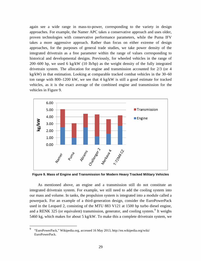
The combined mass per unit power (kg/kW) for the engines and transmissions used in some comparable combat vehicles of the same weight class is shown in Figure 9. We

28

again see a wide range in mass-to-power, corresponding to the variety in design approaches. For example, the Namer APC takes a conservative approach and uses older, proven technologies with conservative performance parameters, while the Puma IFV takes a more aggressive approach. Rather than focus on either extreme of design approaches, for the purposes of general trade studies, we take power density of the integrated drivetrain as a free parameter within the range of values corresponding to historical and developmental designs. Previously, for wheeled vehicles in the range of 200–600 hp, we used 6 kg/kW (10 lb/hp) as the weight density of the fully integrated drivetrain system. The allocation for engine and transmission accounted for 2/3 (or 4 kg/kW) in that estimation. Looking at comparable tracked combat vehicles in the 30–60 ton range with 800–1200 kW, we see that 4 kg/kW is still a good estimate for tracked vehicles, as it is the exact average of the combined engine and transmission for the vehicles in Figure 9.

Figure 9. Mass of Engine and Transmission for Modern Heavy Tracked Military Vehicles

As mentioned above, an engine and a transmission still do not constitute an

integrated drivetrain system. For example, we still need to add the cooling system into our mass and volume. In tanks, the propulsion system is integrated into a module called a powerpack. For an example of a third-generation design, consider the EuroPowerPack used in the Leopard 2, consisting of the MTU 883 V121 at 1500 hp turbo diesel engine, and a RENK 325 (or equivalent) transmission, generator, and cooling system.9 It weighs 5460 kg, which makes for about 5 kg/kW. To make this a complete drivetrain system, we

9 “EuroPowerPack,” Wikipedia.org, accessed 16 May 2013, http://en.wikipedia.org/wiki/ EuroPowerPack.

29

only need add the weight of the final drives that connect the powerpack output to the sprockets that drive the tracks. Based on final drives for three representative vehicles, the M1, M2, and M113, as listed in Table 12, we find the mass of a pair of final drives also scales linearly with power, at about 0.8 kg/kW.

Table 12. Final Drives for Tracked Vehicles

Vehicle Power (kW) Mass of Final Drives (2, kg)

M113a 175 160 M2b 373 347 M1b 1120 854

Sources: a Materials for Lightweight Military Combat Vehicles, Report of the Committee on

Materials for Lightweight Military Vehicles, National Materials Advisory Board, Commission on Engineering and Technical Systems, National Research Council Publication NMAB-396 (Washington, DC: National Academy Press, 1982), 42–43.

b ”Introduction to the X110-3B Transmission, M1A1 Abrams Tank”, Subcourse OD1710, Edition A, Aberdeen, MD: United States Army Ordnance Center and School, Nov. 1991, 60.

Adding this to the powerpack, we get a total specific power for the drivetrain of 5.8

kg/kW, which is very close to our previously established wheeled vehicle rule of thumb of 6 kg/kW (10 lbs/hp). Note that even with the power pack design, there are components associated with drivetrains that are not accounted for—for example, air intake and filtration systems. We also need to account for mounting systems, etc., such that a rough rule of 6 kg/kW seems to be a good estimate for well-established technologies. For developmental technologies, the power density may be able to be reduced to 5 kg/kW. In the sensitivity study, we will see that the gain for changes in the powerpack density is 0.17 (meaning a 1 percent change in specific power changes the overall vehicle weight by 0.17 percent) , so a 17 percent reduction, from 6 kg/kW to 5 kg/kW, could reduce the overall weight of the vehicle by about 3 percent.

In conclusion, we find that the relationship between the weight of the integrated drivetrain and the rated power is approximately linear over the range of interest up to about 1200 kW, and that a specific power of 6 kg/kW is a reasonable estimate for mature technology, while as low as 5 kg/kW might be possible using advanced, but available technology. Furthermore, the advanced technologies discussed as examples are operating in a new regime of engine stress that carries some risk of accelerated failure rates or maintenance issues we cannot fully assess at this time, but should be considered with caution.

30

6. Volume of Drivetrain Components

The interior volume occupied by drivetrain components is critically important for tracked combat vehicles because it is usually protected by armor, so the greater the volume, the more armor weight, which increases the required power, etc. We estimate that, like weight, the volume scales approximately linearly with weight by geometric similarity, and that weight scales linearly with power. Unfortunately, we were unable to find a good set of data to derive an empirical correlation with power. We have, however, already shown that we can reasonably predict the mass of the drivetrain. The volume occupied by that mass depends on the degree to which the components are integrated to eliminate any wasted space. Comparing the mass-to-power estimate to the volume-to-power above of 6 kg/kW, we see that the current state of design achieves an average density of 6 kg/5 L or a net density of 1200 kg/m3, slightly greater than water, and considerably more than typical equipment—for example, as listed in Table 4 with an average of 700 kg/m3. Looking at Figure 10, one can readily see that the design is already very efficient it its use of space, at it seems unlikely that it could be made significantly more compact than this.

Source: MTU.com, accessed 23 July 2013, http://www.tognum.com/press/press-releases/presse-detail/news/mtu_exhibits_drive_systems_for_military_vehicles_at_the_eurosatory/news_smode/images/cHash/b901c699d97b8bf8d0d24b1e7a37ebfa/

Figure 10. MTU EuroPowerPack

31

For the purposes of the model, the drivetrain volume-to-power ratio can be treated as a design parameter and updated if accurate data can be found. In the rest of this discussion, however, we adopt 5 L/kW (0.12 ft3/hp) as a rough estimate, based on the following arguments:

• It should scale directly with mass.

• Its net density represents the state-of-the-art in component integration.

• It is representative of the value of modern design such as the MTU EuroPowerPack

32

7. Volume and Weight Allocations for Power Plant, Drivetrain, and Fuel

Now that we have a method to estimate the weight and volume requirements for the power plant, drivetrain, and fuel, we can generalize these rules in terms of just two performance parameters: power-to-weight ratio and range:

𝑊𝑝𝑝[kg] = �kgkW

�𝑝𝑝

× �Wkg�𝑟𝑒𝑞

× 𝐺𝑉𝑊[kg]

1000

𝑊𝑓𝑢𝑒𝑙[kg] = 𝑅[miles]

𝑡𝑜𝑛 ⋅ 𝑚𝑝𝑔×

3.2 kggal

×𝐺𝑉𝑊[kg]

907 kg/ton

𝑉𝑝𝑝[m3] = �Wkg�𝑟𝑒𝑞

× �L

kW�𝑝𝑝

×𝐺𝑉𝑊[kg]

106

𝑉𝑓𝑢𝑒𝑙[𝑚3] = 𝑊𝑓𝑢𝑒𝑙[kg] × m3

840 kg

where the subscript “pp” stands for powerpack.

The last two expressions can be used to determine the length and subsequently the weight of the structure and armor to protect the power plant, drivetrain, and fuel. Define the weight fractions as:

𝛼𝑝𝑝 = 𝑊𝑝𝑝

𝐺𝑉𝑊

𝛼𝑓𝑢𝑒𝑙 = 𝑊𝑓𝑢𝑒𝑙

𝐺𝑉𝑊.

As well, define the following volume fractions:

𝛽𝑝𝑝 = 𝑉𝑝𝑝𝐺𝑉𝑊

𝛽𝑓𝑢𝑒𝑙 = 𝑉𝑓𝑢𝑒𝑙𝐺𝑉𝑊

.

We will need these fractions later when we use the performance parameters to determine the overall size and weight of the vehicle.

33

8. Weight of Turret

The weight of the turret itself depends on the caliber of the main and secondary weapons, how much ready ammunition is required, automatic feed, drive motors, electronics and sensors. The details would depend on the specific application. For a design tool, however, we can survey modern turrets with approximately the same overall specifications that would be appropriate for an IFV, namely:

• 30 mm auto-cannon, 200 ready rounds

• 7.62 mm coaxial machine gun, 600 ready rounds

• Periscope sights, low-level light, infrared sensors

• Laser rangefinder

• Anti-tank guided missile (ATGM) with 2 ready rounds

• Integral protection against 7.62x51 mm AP rounds

Table 13. Turrets in the Range of 25–30 mm Autocannon with 7.62 mm Coaxial Guns

Model Manning Combat Weight (kg)

Rafael OWS-25Ra 0 1000 SHTURMb 0 1300 Rafael Samson RCWS-30c 0 1500 Giat TMC-25b 1 1600 Nexter Dragar (VBCI)d 1 2000 Rheinmetall E8b 1 2450 OTO Melara HITFIST 30b 2 2670 Rheinmetall (KuKa) E4b 2 3175 Sources: a “Overhead Weapon Station for 25 mm Cannon and Anti-Tank Missiles,” Rafael

Advanced Defense Systems Ltd., accessed 06 May 2013, http://www.rafael.co.il/marketing/SIP_STORAGE/FILES/0/ 540.pdf.

b E. Po, “Turrets for AIFVs: Notes on Current Development and Procurement Programmes,” Military Technology MILTECH 12/2007, accessed 06 May 2013, http://www.epicos.com/WARoot/News/ TurretsforAIFVs.pdf.

c “Samson Mk II RWS Enhanced Survivability Multiple Weapon Station,” Rafael Advanced Defense Systems Ltd., accessed 06 May 2013, http://www.rafael.co.il/marketing/SIP_STORAGE/FILES/7/ 1267.pdf.

d “Dragar,” Deagel.com, accessed 06 May 2013, http://www.deagel.com/Weapon-Stations/ Dragar_a001566001.aspx.

35

If we plot the combat weight of the turrets given in Table 13 against the number of

operators, we find a simple relationship can be used as an approximation, shown in Figure 11. There is substantial variation is exact configurations, but on average the weight is linear with respect to the number of operators, as one would expect.

Figure 11. Combat Weight of Turrets vs. Number of Operators

36

9. Weight of Suspension Components

At first glance, one might suspect that tracked and wheeled suspension systems are so different that design rules of thumb would be substantially different. However, in practice, the same rules seem to apply to both. For wheeled vehicles, we asserted that the total weight of the suspension system should be a fraction αsusp about 1/7 to 1/6 (14–17 percent) of the GVWR, the maximum rated loading. Before we compare this with historical data, let us review some reasons why it is reasonable to expect that the weight of a tracked vehicle’s suspension components should scale linearly with vehicle weight.

If we fix the vehicle width, there are two ways in which the vehicle weight may increase: adding mass for a given length, or adding length. In the case of the latter, one can add additional suspension components by lengthening the track, adding road wheel assemblies, etc., all of which leads to a linear increase in weight, provided we smooth over the discrete nature of these components. While that argument seems simplistic, we also note that in a conceptual design like this, none of the components is fixed yet, and one could imagine simultaneously reducing the size of the existing road wheels—consistent with their expected loading—while adding additional ones such that the overall transition is smooth. If the weight of the vehicle is increased without a length change, e.g., by increasing the force protection requirements, we must look at changes to the various components.

The largest component is the track itself, usually accounting for at least half the weight of the suspension system. For example, the Abrams tracks weigh 10,800 lb out of a total of 20,240 lb for all the suspension components. The track should be chosen to provide a reasonably low ground contact pressure (weight of vehicle divided by contact area of the tracks). Although we do not attempt to prove it here, it is well known that most of the major mobility metrics such as cross-country speed and gradeability can be related directly to contact pressure. For example, high contact pressure leads to sinkage, which increases the resistance to motion and therefore decreases the maximum speed. Likewise, high contact pressure almost always results in a lower drawbar pull-to-weight ratio, therefore reducing the maximum grade than can be climbed for a given soil strength. This observation leads to the design conclusion that track area should increase proportionally to weight in order to maintain a certain value of contact pressure. Without changing the thickness of the track shoes, this can be done by increasing the track width, which will lead to a linear increase in the track mass. Thickness need not be increased because we are constraining contact pressure, the major driver of thickness.

37

We continue by looking at simple structures that might constitute a suspension system. The next largest weight contributor is the road wheels. As a simple structure, we are looking a rigid wheel under load applied at its axle. Since there is some sinkage, a portion of the wheel’s circumference will be in contact with the ground via the track shoe(s). If we assume the track is perfectly flexible, one can estimate the sinkage by:10

𝑧0 = 6 𝑊

5 𝑏 𝑘 √𝐷

where W is the load on the axle, b is the wheel width, k is a coefficient of proportionality that relates the pressure in the ground as a function of depth (for Berstein’s condition where 𝑝 = 𝑘𝑧1/2), and D is the wheel diameter. One can maintain a constant sinkage value by either making b or √𝐷 proportional to load, either of which will lead to a linear increase in mass.

Finally, we make one more analysis on general support structures. Consider an idealized I-beam with cross-sectional area a in the flanges separated by a web of height h, simply supporting a distributed load. For a given beam length, the peak deflection is inversely proportional to the moment of inertia of the cross-section,11 𝐼 = 𝑎ℎ2/4. Therefore, to maintain the same deflection under increasing load, assuming the overall dimensions cannot change, one would have to linearly increase the cross-section, thereby increasing the beam’s mass proportionally to the load.

There are a few counter examples to this general scaling assertion—for example, the torsion bar often used as suspension springs, which tends to scale in mass proportionally to the square root of the load, under the assumption that one desires the same performance in terms of vertical deflection and resonant frequency. For coil springs, the situation is more complicated, depending on which dimensions are adjusted. However, these components are not major drivers of the overall system weight. To summarize the arguments for a linear scaling of suspension components with vehicle weight:

• The major components, such as tracks and road wheels, can be shown using basic engineering relationships to follow linear scaling with weight when their major performance characteristics are left unchanged.

• Basic structures like beams can be shown to have a linear scaling with load when their performance characteristics are left unchanged.

10 M. G. Bekker, Theory of Land Locomotion: the Mechanics of Vehicle Mobility (Ann Arbor, MI: The University of Michigan Press, 1956), 242.

11 T. Avallone, T. Baumeister, III, and A. Sadegh, Marks’ Standard Handbook for Mechanical Engineers, 11th Ed. (New York, NY: McGraw Hill, 2007), Tables 5.2.2 and 5.2.6.

38

• For changes in weight related to weight, suspension components can be duplicated in a linear fashion that also results in a linear scaling with vehicle weight.

• Counter-examples to linear scaling, such as torsion rods, account only for a small fraction (< 10%) of the total system weight.

Therefore, we assume that the total weight of suspension components, in the absence of design detail, is roughly proportional to vehicle weight. We now try to establish what fraction to allocate.

For wheeled vehicles, we found that 14–17 percent was a reasonable estimate. We have limited data for tracked vehicles; however, we strongly suspect the same kind of general trend with the development year in which modern designs have tried to minimize weight wherever possible. For older military tracked vehicles, for example in 1979, the M113-A2 was rated for 25,000 lb, while the total weight of the suspension system was 5,439 lb (22 percent).12 By 1992, however, the M1A2 Abrams, rated at 139,000 lbs, had a total suspension system (with the T158LL track) that weighed 20,240 lb (16 percent).13

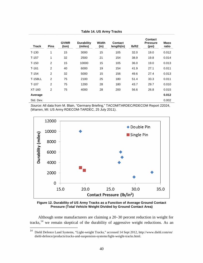
As the tracks are a major contributor to the weight, we should examine them in some detail with regard to scaling and development efforts. Data for various US Army vehicle tracks is shown in Table 14.

12 Committee on Materials for Lightweight Military Vehicles, National Research Council (US), National Materials Advisory Board, “Materials for lightweight military combat vehicles,” Publication NAMB-396 (Washington, DC: National Academy Press, 1982).

13 G. Hintz, J. Pytleski, and D. Rock, “The Design, Development and Fabrication of MlAl Composite Roadwheels,” US TACOM Report 13525 (Warren MI: US Army Tank-Automotive Command, 30 April 1991); T. Balliett, “Investigation of Cast Austempered Ductile Iron (CADI) Trackshoes in T-158 Configuration,” US TACOM Report 13575 (Warren, MI: US Army Tank-Automotive Command, 03 Jan 1992). Some component weights were estimated.

39

Table 14. US Army Tracks

Track Pins GVWR (ton)

Durability (miles)

Width (in)

Contact length(in) lb/ft2

Contact Pressure

(psi) Mass ratio

T-130 1 15 3000 15 105 32.0 19.0 0.012

T-157 1 32 2500 21 154 38.9 19.8 0.014

T-150 2 15 10000 15 105 36.0 19.0 0.013

T-161 2 40 6000 19 154 41.9 27.1 0.011

T-154 2 32 5000 15 156 49.6 27.4 0.013

T-158LL 2 75 2100 25 180 51.4 33.3 0.011

T-107 2 75 1200 28 180 43.7 29.7 0.010

XT-160 2 75 4000 28 200 56.6 26.8 0.015

Average 0.012

Std. Dev. 0.002

Source: All data from M. Blain, “Germany Briefing,” TACOM/TARDEC/RDECOM Report 22024, (Warren, MI: US Army RDECOM-TARDEC, 25 July 2011).

Figure 12. Durability of US Army Tracks as a Function of Average Ground Contact

Pressure (Total Vehicle Weight Divided by Ground Contact Area)

Although some manufacturers are claiming a 20–30 percent reduction in weight for tracks,14 we remain skeptical of the durability of aggressive weight reductions. As an

14 Diehl Defence Land Systems, “Light-weight Tracks,” accessed 14 Sept 2012, http://www.diehl.com/en/ diehl-defence/products/tracks-and-suspension-systems/light-weight-tracks.html.

40

example of track weight vs. durability, consider that single-pin tracks generally weigh about 75 percent of the equivalent double-pin track on a per-square-foot basis (e.g., compare the Bradley T161 to the Abrams T158LL). However, it is widely accepted that double-pin tracks have superior durability, as illustrated in Figure 12. Note that durability drops as the average contact pressure CP (GVW divided by ground contact area) increases and that double-pin tracks do better than single-pin tracks for the same contact pressure. Most modern tracks are exclusively double-pin. Figure 13 and Figure 14 illustrate the difference between single- and double-pin track construction.

Figure 13. Single-pin Track Construction

Using Abrams as an example of a double-pin design, the track has an areal density

psftrk = 52 lbs/ft2. The fraction of track in contact with the ground is always about 1/3 (derived by looking at illustrations and other data). We know that most off-road mobility is a function of average contact pressure. A good value of CP is 15 psi or less. Inputs to mobility simulations such as NRMM II use vehicle cone index (VCI), which is directly related to average contact pressure, as we have shown previously.15 Combine the mobility parameter with our rule of thumb, we can quickly estimate the total weight of the tracks:

𝑀𝑡𝑟𝑘 = 3 𝑝𝑠𝑓𝑡𝑟𝑘 𝐺𝑉𝑊144 𝐶𝑃

.

15 Gillingham, IDA Document NS D-3747.

41

For example, at 15 psi and GVW = 140,000 lb, the tracks should weigh 10,100 lb using our rule. For comparison, note that the Abrams tracks weigh a total of 10,725 lb.

However, the track areal density is correlated with the contact pressure. In fact the ratio of the weight per square foot of the track to the weight of the vehicle per square foot on the ground over all kinds of tracks is 0.012 ± 0.002. Combining this ratio into the formula for the weight of the track, we find the weight of both tracks is about 6 x 1.2 percent = 7.2 percent of the GVW. The Abrams tracks are rated for 75 tons, so they should weight 10,800 lb, using this rule, which is almost exactly what they do weigh.

Figure 14. Double-pin Construction

42

10. Determination of Gross Vehicle Weight and Size

Now that we have established a program for sizing the protected volume as well as the propulsion and suspension systems, we can determine the overall vehicle weight. The GVW will be determined by two components: one that is fixed by the turret and cabin that contains the crew, passengers, and payload, represented by 𝑊0, and one that scales proportionally with the GVW, including propulsion and suspension. Symbolically,

𝐺𝑉𝑊 = 𝑊0 + 𝑊′𝐺𝑉𝑊 ,

where 𝑊′ is the ratio of GVW for suspension and propulsion (including fuel), including associated support structure and protection. To determine the GVW, we must collect a variety of inputs that fall into three categories—basic dimensions, empirical factors, and requirements—as shown in Table 15, along with their recommended values where applicable.

The crew, passenger, and protected payload capacity will set the length of the cabin. In our model, we have fixed the cross-section in a way that accommodates a proportionally appropriate amount of payload. If there is a payload requirement that is fixed regardless of the size of the crew and passengers, we can estimate the cabin length for that portion also using our cargo packing rule of thumb, e.g., 560 kg/m3.

43

Table 15. Necessary Inputs for a Notional IFV Design Using the Method Described in this Paper

Symbol Description Recommended

Value

Basic Dimensions wp Width of personnel cabin 91 cm wob, max Maximum width of outboard storage space 64 cm hp Height of personnel cabin 152 cm hob Height of outboard storage space 100 cm θ Angle of v-hull 25o ht Height of turret 61 cm dt Diameter of turret 150 cm

Empirical Factors αA,B,C Fraction of weight required for support by kit type (A, B or C) 0.1/0.05/0.2 kg/kW Fully integrated power plant and drivetrain weight density 6 kg/kW L/kW Power plant and drivetrain volume density 5 L/kW αsusp Fraction of GVWR for suspension components 0.14 ρequip Packing density of mission-related and auxiliary automotive

equipment 560 kg/m3

Performance Requirements PL Total payload, including auxiliary automotive, mission-

related equipment, crew, and passengers n/a

Wpv,0 Weight of fixed auxiliary automotive and mission-related equipment to be placed inside protected volume

n/a

W’pv Additional auxiliary automotive and mission-related equipment to be placed inside the protected volume per passenger

n/a

Ncrew Number of crew members n/a Npax Number of passengers n/a Wturr Weight of turret, excluding armor or generic turret type n/a W/kg Power-to-weight ratio (derivable from mobility requirements) n/a R Maximum range for a given mission profile (fractions and

rolling resistance) n/a

λI, j Set of armor areal density for surfaces i and kit levels j n/a

The personnel cabin has cross-sectional area Ap = wp hp. The length of the protected cabin can be determined from:

𝑙𝑐𝑎𝑏𝑖𝑛 = 𝑁𝑐𝑟𝑒𝑤 𝑉𝑐𝑟𝑒𝑤+𝑁𝑝𝑎𝑥 𝑉𝑝𝑎𝑥𝐴𝑝

.

44

The cross-sectional area of the under-floor space, which includes such items as supplies, electronics, auxiliary automotive components (e.g., pneumatics), and air conditioning is:

𝐴𝑢𝑓 = 14𝑤𝑝2 tan𝜃.

The weight of auxiliary automotive and mission-related equipment to be stored in the protected volume is:

𝑊𝑝𝑣 = 𝑊𝑝𝑣,0 + 𝑊𝑝𝑣′ 𝑁𝑝𝑎𝑥 .

The portion of this weight that can be accommodated by the under-floor volume is:

𝑊𝑝𝑣,𝑢𝑓 = 𝐴𝑢𝑓 𝑙𝑐𝑎𝑏𝑖𝑛 × 280 kg/m3 .

The remaining portion of the protected payload must go into the outboard volume. We expand the width of the outboard storage to accommodate it, out to the maximum allowed width. The width required can be calculated by:

𝑤𝑂𝐵 = 𝑊𝑝𝑣−𝑊𝑝𝑣,𝑢𝑓

𝐴𝑜𝑏 ,

where:

𝐴𝑜𝑏 = 2 ℎ𝑜𝑏 𝑙𝑐𝑎𝑏𝑖𝑛 .

If the width calculated in this manner exceeds the maximum allowed wob,max, the cabin length must be increased to accommodate the additional weight.

Once the cabin length lcabin is set, we can determine the surface areas of the sides, top, bottom, under the outboard storage, front and back:

As i d e =2 l0 hp

At o p = l0 (wp+ 2 wo b)

Ab o t t o m = l0 wp /cosθ

Au n d e r =2 l0 wo b

𝐴𝑓𝑟𝑜𝑛𝑡/𝑏𝑎𝑐𝑘 = 𝑤𝑝 ℎ𝑝 + 2 𝑤𝑜𝑏 ℎ𝑜𝑏 + 14𝑤𝑝2 tan𝜃

𝐴𝑡𝑢𝑟𝑟 = 𝜋 𝑑𝑡 ℎ𝑡 .

The labels should be self-explanatory, except perhaps “under,” which refers to the surface beneath the outboard storage compartments. This is separated from the underbody hull

45

(V-hull) because its location above the tracks may have a different protection requirement.

For a given threat protection level and armor solution (e.g., rolled homogeneous armor (RHA)) one can determine the areal density (kg/m2), denoted by the symbol λ, for use in calculations. Since we may have a different requirement for each surface, we annotate each with a subscript i,j where i indicates the surface, and j indicates the kit level (A, B, or C). In Appendix D, we illustrate a scaling of areal density (or thickness) for metallic armors based on a simple threat metric for armor-piercing rounds. Otherwise, one may use the results of threat-specific armor solutions, e.g., ceramic over composites. For underbody protection against mines, one needs to use a specific solution, as we have not been able to derive accurate scaling laws. We also include a fraction α of the armor weight for support and attachment. These factors vary by kit level as follows:

• αA = 0.1, to account for monocoque hull support (joints, weldments, support framing, etc.)

• αB = 0.05, to account for mounting fixtures to existing surfaces, e.g., attaching applique armor

• αC = 0.2, to account for extended structures to support supplemental armor (typically, the C-kit mounts far outboard)

The basic integral hull must provide A-kit level protection and have the support structures for the B and C kits; therefore, the weight of the integral hull is:

𝑊ℎ𝑢𝑙𝑙 = ∑ 𝐴𝑖�(1 + 𝛼𝐴)𝜆𝑖,𝐴 + 𝛼𝐵𝜆𝑖,𝐵 + 𝛼𝐶𝜆𝑖,𝐶�𝑖 ,

where the summation is over all the surfaces of the hull, i.e., sides, top, bottom, under, front, and back. The additional weights of the other kits are:

𝑊𝐵 = ∑ 𝐴𝑖𝜆𝑖,𝐵𝑖

𝑊𝐶 = ∑ 𝐴𝑖𝜆𝑖,𝐶𝑖 .

Note that the weight of the C-kit is not included in the GVW. However, the vehicle must be able to support the total weight including the C-kit. We denote the total supportable weight as GVWR (GWV rating). The scaling of the propulsion plant including fuel is computed at GVW, i.e., the performance requirements apply to the B-kit configuration at full payload. This means that the suspension part separates into two parts: one that scales with GVW and one that is fixed by the additional C-kit weight. This can be absorbed into the fixed weight:

𝑊0 = 𝑊ℎ𝑢𝑙𝑙 + 𝑊𝑡𝑢𝑟𝑟 + 𝑊𝐵 + 𝛼𝑠𝑢𝑠𝑝 𝑊𝐶 + (1 + 𝛼𝐵)𝑃𝐿,

46

where Wturr is the weight of the turret without additional armor protection, and PL is the total amount of payload, internal or external, including auxiliary automotive equipment and personnel. Note that the additional structure to support the payload is treated as if it were a B-kit, in the sense that it typically involves attaching items to existing structure, e.g., floors, walls, or ceiling. If a large amount of equipment needs to be mounted outside of the cabin, beyond the capacity of hanging onto the existing structure, one would need to account for a separate structure, e.g., a truck bed, in which case it would be more appropriate to use a similar parasitic weight fraction like the A-kit, i.e., 10 percent or more.

The remaining complication is to account for not only the direct weight but the weight of the protection and support required to house the power plant and fuel. Since we know how the volume scales with performance requirements, we simply need to convert the protected volume into the various areas. If the cross-sectional area does not change from the cabin design, we can reuse our earlier work and compute the weight per unit length, 𝑊ℎ𝑢𝑙𝑙/𝑙0. The length is found by dividing the volume requirement (per kg of GVW) by the cross-sectional area, Ap + 0.5 Auf + Aob, where we have again assumed one can only use half of the under-floor space. Adding up all the items that contribute to the weight that scale with GVW—the weight of the power plant, drivetrain, fuel, suspension, and the additional structure and armor to protect the power plant, drivetrain, and fuel—the term for the fraction of GVW is:

𝑊′ = 𝛼𝑝𝑝 + 𝛼𝑓𝑢𝑒𝑙 + 𝛼𝑠𝑢𝑠𝑝 + 𝑊ℎ𝑢𝑙𝑙𝑙0

(𝛽𝑝𝑝+𝛽𝑓𝑢𝑒𝑙)(𝐴𝑝+0.5𝐴𝑢𝑓+𝐴𝑜𝑏)

.

Having defined all the expressions, this allows us to compute the GVW in a single expression:

𝐺𝑉𝑊 = 𝑊01−𝑊′

,

where all the terms on the right can be derived from basic performance requirements and the level of protection, subject to some basic shape assumptions and constraints. The calculation can be easily done in a simple spreadsheet or programmed in MATLAB for creating detailed trade study plots.

47

11. Summary

The method described in this paper illustrates how one can determine most of the basic design parameters of an IFV based on only a few major performance parameters. This should allow one to easily make trade studies among the performance parameters without much difficulty. Although we have provided recommended values for all of the basic dimensions and empirical factors necessary to estimate the vehicle design, these too can be modified if desired, keeping in mind the constraints and developmental risks as noted previously.

49

Appendix A. Sensitivity Study

We begin with a Bradley-like (M2A3) configuration, which our model predicts will weigh about 69,700 lb GVW. The assumptions are:


• 14.5 mm at 300m integral 360 degree protection

• 40 psf applique on sides, front, back, and turret sides (B-kit)

• 21.5 ft overall length, 81″ tall (turret top), 102″ wide

• Payload 4655 lb (not including turret and ready ammo)

Next we vary the major design parameters by 1 percent and note the change in output on GVW shown in Table A-1. Comparing the percentage gives us a measure of the relative gain. Additionally, we vary the turret-manning assumptions in order to see the magnitude of the effect this has on the overall vehicle.

A-1

Table A-1. Changes in GVW as a Function of a 1% Change in Various Input Parameters

Parameter Change Change in GVW (lb) Percent Change (%)

A-kit psf, 58 psf +0.58 psf +576 +0.83 Hp/ton, 20 +0.2 hp/t +297 +0.43 B-kit psf, 40 psf +0.4 psf +225 +0.32 Cabin width, 60” +0.6” -212 -0.30 Vol per passenger (6), 30 ft3

+0.30 ft3 + 179 (30 each) +0.26 (0.04 each)

Suspension percent of GVW, 14.3%

+0.14% +173 +0.25

Turret diameter, 72” +0.72” +159 +0.23 Vol per crew(3), 35 ft3 +0.35 ft3 +139( 46 each) +0.20 (0.07 each) Powertrain density, 10 lb/hp

+0.1 lb/hp +121 +0.17

Turret height, 24” +0.24” +79 +0.11 Density of equipment, 35 lb/ft3

+0.35 lb/ft3 -66 -0.09

Outboard height, 30” +0.3” -51 -0.07 Range, 200 miles +2 miles +44 +0.06 Cabin height, 50” + 0.5” -39 -0.06 Weight of aux auto/integration, 700 lb

+7 lb +26 +0.04

Weight of a person (9), 215 lb

+2.1 lb +23 (2.5 each) +0.03 (-0.004 each)

Turret manning 1 (from 2) -7652 -11.0

Turret manning RWS (2 to 0) -9356 -13.4

A-2

Appendix B. Derivation of Cooling Fan Power vs. Engine

Output Scaling

In order to capture how an IFV will scale with mobility, we also have to compute the cooling power required for the engine. In this appendix, we derive the cooling fan power required as a function of engine power output. First, we assume that the amount of waste heat generated by the engine is proportional to its output. This is probably not accurate over the entire range of engine output; however, once an engine is operating at an appreciable fraction of its full capacity, its operating efficiency tends to be constant. As evidence, consider the brake efficiency of the V-12 diesel engine (developed for the Advanced Integrated Propulsion System by Cummins) as a function of percentage of full load as shown in Figure B-1Error! Reference source not found..

Source: Blue Ribbon Committee, “Research Needed for More Compact Intermittent Combustion Propulsion Systems for Army Combat Vehicles,” Interim Report TFLRF No. 296, US Army Tank-Automotive Research, Development and Engineering Center Fuels and Lubricants Research Facility (SwRI) (San Antonio, TX: Southwest Research Institute, Nov. 1995), 47.

Figure B-1. Engine Brake Efficiency of Developmental Turbo-diesel Engine as a Function of Power Loading

B-1

One can compute the efficiency from the brake-specific fuel consumption (bsfc), which is the rate of fuel consumption divided by the power output. The typical unit for bsfc is g/kWh (lb/h/hp). This can be compared directly to the energy content of fuel. For example, diesel fuel #2 contains 46.2 MJ/kg, which in units of bsfc-1 is 0.0128 kWh/g. The engine brake efficiency can be computed by this relationship:

𝜂 = 1𝑏𝑠𝑓𝑐[g/kWh] ×0.128 kWh/g

.

Using this relationship to compute the efficiency from bsfc as a function of power (at optimum rpm), we see that when power is above 50 percent load, the efficiency is essentially constant up to 100 percent, and only really falls off below 30 percent load.

This is an idealized case, where we have chosen to operate the engine at the rpm that minimizes bsfc at every value of loading. In reality, there are a fixed number of gear ratios available such that, for a given speed, the engine speed cannot always be chosen optimally. The ideal situation would require a continuously varying transmission, which is not common. Also, other frictional losses (e.g., heat transferred to oil) tend to become slightly larger on a percentage basis at high power. These deviations from the ideal case affect the accuracy when making the simplifying assumption that the fraction of energy that goes into heat is also constant; however, the deviation from a linear scaling might only be on the order of 10–20 percent at full load relative to 30 percent loading.

For the cooling system that is ultimately cooled by air, the heat removal capacity is a linear function of �̇�, the air mass flow rate through the radiator. We have made the assumption that the maximum air temperature rise is fixed by the system design. Since the heat that needs to be removed is proportional to the engine power as discussed above, the fan speed should also be proportional to engine power. The power consumed by the fan is proportional to the speed cubed. Combining these two relations, the fan power is proportional to the cube of the output of the engine. The net output power must be a solution to

1 − 𝛼𝑏2 = 𝑤 ,

where b = Pbhp/Pmax is the output of the engine as a fraction of its maximum brake output, α is the fraction of the output load used for the cooling fan at 100 percent output, and w is the fraction of brake output that can be used for propulsion.

Figure B-2 shows the ratio of brake to propulsion power, 1/w, using a cooling fan max load of 0.15. This type of relation can be used to determine the actual engine load as a function of the propulsion load and therefore relate the road load to the brake-specific fuel consumption. For example if the road load at a given speed is 50 percent of the engine maximum output, the actual engine load including the cooling fan will be 52 percent. As one can see, this type of treatment is especially relevant at high power, where

B-2

only 85 percent of the engine’s rating is available for propulsion. This also indicates that for a given maximum road loading, the engine rating needs to be higher to account for the maximum fan loading by a factor of about 1.2. One could have estimated this by dividing by the fan fraction 1/0.85 = 1.18, which is accurate at full power output, e.g., for maximum theoretical speed calculations, but not accurate at lower powers, e.g., for fuel economy calculations.

Figure B-2. Ratio of Brake Output Power to That Which Can be Used for Propulsion (Brake

Less Fan Power) as a Function of Propulsion Power

B-3

Appendix C. Analysis of Engine Weight Scaling with Power

Rating

To understand how engine weight in this range of power ratings should scale, we first must look at some basic concepts and establish a basic framework for the analysis. The reader should note that this is a high-level description and does not address the myriad of engineering decisions and limitations that affect actual designs. Rather, these details are subsumed into three parameters that characterize an engine in terms of its most basic element, the piston—the piston’s pressure, velocity, and area.

Brake mean effective pressure �̅�𝑏 is defined as the ratio of work done per cycle to the displacement D (cross-sectional area of cylinders times their stroke), 𝑊 = �̅�𝑏𝐷. For a measured output torqueτ, the work done per cycle in a four-stroke engine is 𝑊 = 4 𝜋𝜏, noting that there are two revolutions per cycle (we have explicitly assumed a four-stroke engine). Thus, the brake mean effective pressure for a four-stroke engine is given by:

�̅�𝑏 = 4𝜋𝜏𝐷

.

The term “brake” here refers to the measurement of the torque at the engine output, before the torque converter and transmission. Alternatively, we can express �̅�𝑏 using rated power P, rpm, and displacement D, using convenient units:

�̅�𝑏 [bar] = 1200 𝑃[kW]𝑟𝑝𝑚×𝐷[L]

.

The average piston speed is twice the stroke S divided by the cycle period. If we wish to express this in terms of revolutions per minute rpm, the average piston speed is:

𝑣𝑝[m/s] = 𝑆[m] × 𝑟𝑝𝑚/30.

If we wish to express brake power P in terms of �̅�𝑏, vp,:

𝑃 = k �̅�𝑏𝑣𝑝 𝜋𝐵2𝑁𝑐16

,

where B is the diameter (bore) of the cylinders, Nc is the number of cylinders and k is a constant depending on the units. We can now see that for a given engine configuration and speed the only factors affecting power are brake mean effective pressure and piston

C-1

speed. Increasing either has the effect of increasing the stress on the engine components. For example, increasing the piston speed leads to increase friction losses (heat) and increases the cyclic stress on the piston, piston rod, and crankshaft. The cylinder motion is sinusoidal to the first order of approximation, in which case the peak acceleration can be related to mean piston speed, as we have defined it, by:

𝑎� = 𝜋2𝑣𝑝2

𝑆 .

Therefore, the peak inertial stress on the connecting rod is:

𝜎� = 𝑀𝑝 𝜋2𝑣𝑝2

𝑆𝐴𝑟 ,

where Mp is the mass of the piston assembly (including the connecting rod) and Ar is the cross-sectional area of the rod. If we enforce geometric similarity, where stroke is proportional to the bore B, the rod area is proportional to B2, and the mass of the piston is proportional to SB2, the peak stress will depend only on the mean piston speed and density ρ of the materials used for the piston and rod:

𝜎� ∝ 𝜌𝑣𝑝2 .

The relative contribution from each of the factors in the stress equation depends on the application. Diesels tend to have heavier pistons (Mp) because they operate at high pressures. This adds inertia to the moving components and, as one would expect, diesels tend to respond more slowly than the equivalent gasoline-powered engine. The additional mass also means greater cyclic stresses, so they tend to have lower piston speeds. Mean piston speeds can be coarsely divided into five classes1 as shown in Table C-1.

Table C-1. Classes of Engines Sorted by Mean Piston Speed

Mean piston speed (m/s) Class Application

~8.5 low speed diesel marine power, electric generation ~11 medium speed diesel trains, trucks ~14 high speed diesel automotive ~16 medium speed gasoline automotive

~20–25 high speed gasoline sport automotive, motorcycles

Higher piston speeds also increase the frictional forces, reducing overall efficiency, accelerating wear on the components. The increased cyclic stress should also have a

1 “Mean Piston Speed,” Wikipedia.org, accessed 19 April 2013, http://en.wikipedia.org/wiki/Mean_ piston_ speed.

C-2

direct impact on the lifetime and reliability of the crankshaft, connecting rods, and pistons. These effects can only be mitigated by design measures, manufacturing technologies, and advanced materials, all of which increase the cost.

Increasing �̅�𝑏, although it is not directly meant to represent the pressure in the cylinder, will certainly increase the pressure and temperature in the cylinder leading to increased stress on the materials. If we approximate the cylinder pressure by �̅�𝑏, the averaged hoop stress on the cylinder walls will be:

𝜎𝜃 = �̅�𝑏 �𝐵2𝑡� ,

where t is the wall thickness (assumed to be small compared to diameter B). Therefore, we expect the mass of the engine block to depend approximately linearly on �̅�𝑏 in order to keep the same hoop stress in the cylinder walls. Typical values of �̅�𝑏 for a turbo-boosted diesel are 14–18 bar.2 Values greater than this require more complicated turbo-booster design, perhaps additional stages, and improvements in materials and cooling. These equate to increased cost and, possibly, degraded reliability.

Given these considerations, we examine how engine mass should scale with rated power. For the following arguments, we assume that the engine can be represented by a collection of cylinders with a given bore, height determined by the stroke, and wall thickness determined by the peak pressure. All other elements will scale proportionally based on geometric similarity.

Consider engine power, using the previously derived expression. To increase power, you can increase the following parameters:

• Brake mean effective pressure. Keeping everything else constant, the thickness of the cylinder walls would need to increase proportionally to contain the hoop stress. Just looking at the mass of the cylinders, therefore, we would have a linear increase in mass proportional to �̅�𝑏 and therefore power. The scaling of mass to power would be linear in this case.

• Number of cylinders. This results in a simple linear increase in length, therefore mass, which again is linearly proportional to power. Of course, there are practical limits, and engines exceeding 16 cylinders are rare.

• Displacement. Bore and stroke tend to keep the bore-stroke aspect ratio close to 1 (modern designs are tending to stroke-to-bore ratios of 1.5:1 for various reasons, mostly related to emissions). To keep piston speed the same, the engine speed would have to decrease. Increasing the bore also requires an increase in

2 “Mean Effective Pressure,” Wikipedia.org, accessed 19 April 2013, http://en.wikipedia.org/wiki/Mean_ effective_pressure.

C-3

the wall thickness for hoop stress (thin wall assumption), so the total mass increases proportional to B3 while the power increase is also proportional to B2, so the scaling of mass to power is M ∝ P3/2.

• Piston speed. Higher piston speed increases the stress on the piston connecting the rod and the crankshaft, both of which would need to be made larger. Furthermore, the increased piston speed would increase internal friction losses and volumetric efficiency, which would decrease �̅�𝑏, so we don’t really know the scaling law. However, we observe that most high speed diesels have about the same piston speed, so there appears to be a practical limit on increasing speed. Also, note that increasing the mass of the pistons will increase the inertia and therefore the engine will be less responsive, so there is also a performance impact.

Table C-2. Caterpillar 6-Cylinder Diesel Engines

Model Power (kW) Weight (kg) Ratio (kW/kg)

C6.6 205 506 2.5 C7 224 588 2.6 C9 280 776 2.8 C11 313 930 3.0 C13 388 939 2.4 C15 444 1469 3.3 C18 522 1769 3.4

Source: “Industrial Engine Ratings Guide,” Caterpillar, accessed 10 May 2013, http://www.cat.com/cda/files/ 2208849/7/LEGH0002.pdf.

Since mean piston speed is a function of materials, there really are two types of

scaling: displacement and number of cylinders. For a given configuration, e.g., inline/six-cylinder, keeping �̅�𝑏and vp constant, the only way to increase power is to increase the displacement. This leads to a M ∝ P3/2 scaling law as previously discussed. As an example, consider the seven different models of six-cylinder inline engines from Caterpillar listed in Table C-2. The relationship between power and weight is plotted in Figure C-1. They all have similar mean piston speeds, and therefore the proposed scaling law based on displacement alone explains the variation with a coefficient of determination (R2) of 94 percent.

C-4

Note: All the engines were inline/six-cylinder models. The dashed line is a least-squares fit to a P3/2 scaling

law. The coefficient of determination (R2) is 94%, whereas a linear model has an R2 of 90%.

Figure C-1. Variation of Mass (Dry) of Caterpillar Turbo-charged, Medium-Speed Diesel Engines with Maximum Rating

Because of the scaling of mass with displacement, M ∝ P3/2, at some point it

becomes more beneficial to add cylinders and return to a scaling where M ∝ P, rather than increase displacement. That means the overall scaling will be linear, ultimately accomplished by adding cylinders for more power, and between the points where cylinders are added, the scaling for a given number of cylinders is M ∝ P3/2. This is shown notionally in Figure C-2.

C-5

Figure C-2. Notional Scaling Behavior of Mass of Diesel Engines with Power Rating

C-6

Appendix D. Derivation of Scaling Law for the Minimum Metallic Armor Thickness to Defeat Armor-

Piercing Ammunition

Introduction It should be clear that the dominant factor in determining an IFV’s weight is the

weight of the protective armor. This is especially true as the threat level continues to increase. In models similar to the one described in the main body of this paper, the fidelity is mostly a function of the protection model. Therefore, we will now discuss in detail a model that relates the threat to the thickness, and thereby weight, of the armor needed to protect against it.

Although metallic armor is considered old technology, it may still be a desirable solution for the base armor of ground vehicles because of its relatively low cost, as well as its strength and endurance as a structural component. Additionally, metallic armor has excellent multi-hit performance and serves well as protection from a blast. When combined with applique or add-on armor, it acts in conjunction to provide synergistic protection for threats that cannot be defeated in any practical sense by a single monolithic material. Examples include high-explosive rounds and shaped charges (explosively formed projectile (EFP) and jet).

There is a plethora of data for common armor materials against specific threats. To specify a threat, you need the specific round, perhaps the weapon that fires it, and range, from which you can infer the velocity. An example of such a threat specification is STANAG 4569: Protection Levels for Occupants of Logistic and Light Armored Vehicles, which has five levels. It does not cover all of the possible threats, nor does it cover the effective range of these weapons; it simply states a single combination of ammunition, weapon, and range for each of the five levels. It would be beneficial under some circumstances to have an understanding of the armor’s performance against a generic threat that can be varied over a wide range—for example, to plot contours of protection level against weight for a specific vehicle design.

This appendix demonstrates that there is a simple method to generically specify threats from armor-piercing ammunition that applies to common metallic armors such as rolled homogenous armor (RHA), high-hardness armor (HHA), and titanium (Ti6Al4V). It applies to situations in which the projectile is harder than the armor, such that there is

D-1

little deformation of the projectile and the projectile does not completely penetrate the armor. It will not apply to fragments from artillery shells or improvised explosive devices, as these will typically be of similar hardness and therefore deform. We found that the data for penetration resistance supports a very simple model where the thickness of the armor required is proportional to the square root of the ratio of kinetic energy of the projectile over its diameter. Physically, this relates the resistance of penetration to simple shear plugging, where a cylinder of armor of equal diameter to the projectile (or in some cases, its hardened core) is pushed out a distance equal to the thickness of armor at the ballistic limit. The resistance of the plug from the shear force at the outer surface of the plug provides the force that brings the projectile to rest in the armor. This model was found to have excellent agreement with data over a wide range of projectiles, from 7.62 mm to 90 mm ammunition, covering about two orders of magnitude in the simple threat metric.

Physical Model of Simple Shear Plugging In the regime of interest, that of small-to-medium caliber armor-piercing rounds,

with velocities from about 500 to 1500 m/s, the impact pressure is expected to easily exceed the yield strength of the target. The core of the armor-piercing round is also hardened such that little of no deformation of the projectile occurs during penetration at these velocities. This is an assumption, and would require that the yield strength of the penetrator be more than three times the yield strength of the target (using the stress intensification factor of three), which is not strictly true, especially for high or ultra-high hardness steels. However, for finite thickness plates, it does not really affect the results, as will be demonstrated by the empirical evidence.

For finite thickness plates, the structure of the plate cannot necessarily bear the net thrust of the impact and penetration. The response of the plate may be to bend, bulge, petal or plug, among others. The empirical data can be supported in many cases by the simplest model, namely that of simple shear plugging.

For simple shear plugging, we again equate the kinetic energy of the projectile to the work done pushing out the cylindrical plug at some resistance of the material to shearing τY, which one can assume is equal to 𝜏Y = 0.7 𝑈𝑇𝑆 where UTS is the ultimate tensile strength.1 We have assumed that there is no additional energy, e.g., in the form of a chemical explosive, and that the projectile fully expends its energy in the plate. The force changes as the plug separates, so one needs to integrate over depth in the armor.

1 S. Kalpakjian and S. Schmid. Manufacturing Engineering and Technology (Prentice Hall: Englewood Cliffs, NJ, 2005), 450.

D-2

The result for the ballistic limit thickness is:

𝑡𝐵𝐿 = � 𝑚𝑣2

0.7 𝑈𝑇𝑆 𝜋𝐷�1/2

,

where D is the diameter of the projectile.

Rolled Homogeneous Armor (MIL-DTL-12560J) Ballistic Limit We collected data on thickness of RHA for penetration resistance (V50) for

projectiles ranging from 7.62 mm to 90 mm. This data is shown in Table D-1.

D-3

Table D-1. Thickness of RHA at Ballistic Limit for Various Projectiles

Projectile Mass (g) Diameter

(mm) Velocity (m/s) Thickness (mm)

7.62x39 mm API BZ 7.8 7.6 404 5.1a 7.62x54R API (B32) 10.2 7.9 434 5.1a 0.30 cal AP (M2) 5.3 6.2 460 5.8b 0.30 cal AP (M2) 5.3 6.2 427 8.4a 0.50 cal AP (M2) 25.4 10.3 421 10.9c 7.62x39 mm API BZ 7.8 7.6 726 12.3a 0.50 cal AP (M2) 25.4 10.3 580 15.4b 0.30 cal AP (M2) 5.3 6.2 820 16.5a 0.30 cal AP (M2) 5.3 6.2 866 16.5b 7.62x54R API (B32) 10.2 7.9 877 17.0a 0.50 cal AP (M2) 25.4 10.3 654 21.0c 20.35 x 203.45 mm

Bearcatd rod 454 20.4

381 25.4e 20x139 API (DM43) 77.0 12.6 582 30.2b 2.79 x 81.28 mm U rod 9.1 2.3 1067 31.2e 14.5x114 AP B32 64.0 14.9 779 35.2f 3.81 x 76.2 mm U rod 15.7 3.81 1298 46.7e 20x139 API (DM43) 77.0 12.6 856 50.0g 20.35 x 203.45 mm

Bearcat rod 454 20.4 671 50.8e

3.56 x 76.96 mm U rod 12.4 3.6 1573 66.0e 20x139 API (DM43) 77.0 12.6 1042 72.4b 7.68 x 76.80 mm X9Ch LRP 65.0 7.7 1406 76.2i

90 mm AP-T (M318A1) 11000 90.0 483 100.1b 10.24 x 102.4 mm X9C LRP 154 10.3 1360 101.6i

90 mm AP-T (M318A1) 11000 90.0 519 108.2b 5.30 x 159.10 mm X9C LRP 65 5.3 1385 114.3i

90 mm AP-T (M318A1) 11000 90.0 549 116.1b 90 mm AP-T (M318A1) 11000 90.0 579 124.0b 15.80 x 311.4 mm

Bearcat rod 454 15.8 1547 152.4e

Sources: a W. Gooch and M. Burkins, “Analysis of Threat Projectiles for Protection of Light Tactical Vehicles,”

ARL-RP-89, Army Research Laboratory, 2004. b MIL-DTL-12560J, Detail Specification: Armor Plate, Steel, Wrought, Homogeneous(24 Jul 2009). c Gary's Olive Drab Page 2012, accessed 6 June 2012, http://www.inetres.com/gp/military/index.html. d Bearcat is a hardened tool steel (Bethlehem Steel), approximately Rockwell C hardness 60. e C. L. Grabarek, "Penetration of Armor by Steel and High Density Penetrators," Memorandum Report

No. 2134 (Aberdeen, MD: U.S. Army Ballistic Research Laboratories, Aberdeen Proving Ground, 1971).

D-4

These data points vary in diameter from 7.62 mm to 90 mm, and in kinetic energy

from 635 J to 1.8 MJ. The thickness-to-diameter ratio varies from 0.7 to 21.0. Figure D-1 shows a comparison of the thickness of RHA corresponding to the ballistic limit, where the V50 is defined by MIL-STD 662F2 as “the average of an equal number of highest partial penetration velocities and the lowest complete penetration velocities which occur within a specified velocity spread.…The maximum allowable velocity span is dependent on the armor material and test conditions. Maximum velocity spans of 60, 90, 100, and 125 feet per second (ft/s) (18, 27, 30 and 38 m/s) are frequently used.”

Although we do not assert that the simple shear plug model describes what is happening during penetration, the data over a wide range of parameters fit the dependence on mass, diameter, and velocity very well, with an r-squared of 97 percent. Note that, from a theoretical basis using the simple shear plugging model, the linear coefficient depends only on the UTS of RHA. Note that there is some variation of strength, depending on the plate thickness, but for our purpose we can use a single number, which for RHA is 1170 MPa. The prediction of the simple shear plugging model with this value for strength is also plotted in Figure D-1, and shows remarkable agreement with a linear fit to the data.

Figure D-1. Comparison of RHA Ballistic Limit Thickness to Square Root of Kinetic Energy

over Diameter

2 MIL-STD-662F, Military Standard: V50 Ballistic Test for Armor (18 Dec 1997), Section 3.8.

D-5

Other Materials We can also perform the same type of analysis on other common metallic armor

materials.

High-Hardness Armor (HHA) HHA, as specified in MIL-DTL-46100E,3 was developed to improve the penetration

resistance of wrought steel plate (oil quenched and tempered). The specification allows a range of hardness (Brinell) of 477–534. For our purposes, we assume HB = 500, corresponding to an ultimate tensile strength of 1640 MPa. For comparison, RHA has an average HB = 344, and a strength of 1170 MPa (note this can vary quite a bit, especially with plate thickness, because of the quench process).

There are two types of data points: actual data and acceptance values for MIL-DTL-46100E, which can be treated equivalently as data. They also are further split into those at normal (0 degree) obliquity and those from 30 degree obliquity. Acceptance tests sometimes use 30 degree obliquity to get more consistent results, whereas data at 0 degree obliquity can sometime exhibit a “shatter gap,” where two separate ballistic limit velocities can be found for the same projectile. The higher velocity occurs when the projectile shatters on impact.

Looking at the normal obliquity data (excluding the MIL-DTL-46100E points), the plate thickness seems to follow with the simple plug shear model and lies more or less on a straight line as a function of the square root of the ratio of the projectile’s kinetic energy to its diameter (see Figure D-2).

3 MIL-DTL-46100E, Detail Specification: Armor Plate, Steel, Wrought, High-Hardness (08 Jul 2008).

D-6

Note: Data were limited to hardened projectiles at normal obliquity.

Figure D-2. Plate Thickness at Ballistic Limit for HHA (MIL-DTL-46100E) as a Function of the Square Root of the Ratio of the Projectile’s Kinetic Energy to its Diameter for Normal

Shots

On the other hand, if we include the 30 degree obliquity data, dividing the plate thickness by cos(30o) to account for the increased line-of-sight thickness (and corresponding increase in areal density), we get mixed results, where some points fall on the same line as the 0 degree obliquity and others fall well below. Also shown is the tBL using the simple shear plugging model with the tensile strength of HHA. Note that the model using just strength is within a few percent of the fit to the 0 degree obliquity data, and the data can be represented by a linear function with a very good R2 value of 95 percent. Trying to incorporate the 30 degree obliquity points is not desirable for two reasons: first, there may additional effects related to obliquity that in some cases improves the performance of the armor plate, and second, we want our model to represent a conservative bound. Therefore, we choose a fit to only the 0 degree obliquity data and display the 30 degree obliquity data for comparison only (see Figure D-3).

D-7

Note: Data points for 30 degree obliquity have been multiplied by 1.155 (1/cos30o) to account for the

increased thickness along the projectile’s trajectory. The solid line is a least-squares linear fit, and the dashed line is the simple shear plug model based only on the target strength.

Figure D-3. Plate Thickness at Ballistic Limit for HHA (MIL-DTL-46100E) as a Function of the Square Root of the Ratio of the Projectile’s Kinetic Energy to its Diameter for Normal

and 30-Degree Shots

Ti6AlV Armor, MIL-DTL-46077G This armor has an ultimate tensile strength of 970 MPa, so we expect effects similar

to those of RHA and HHA. Selected points from MIL-DTL-46077G4 are listed along with data points from other sources in Table D-2, and the data is plotted in Figure D-4. Again we have data covering a wide range, with their dependence on the square root of the ratio of the projectile’s kinetic energy to its diameter well represented by a linear fit with an r-squared of 98 percent, and good agreement with the simple plug model based solely on target strength.

4 MIL-DTL-46077G, Detail Specification: Armor Plate, Titanium Alloy, Weldable (28 Sep2006).

D-8

Table D-2. Ballistic Limit Data for Ti-6Al-4V Armor

Projectile Mass (g) Diameter

(mm) Velocity

(m/s) Thickness (mm)

7.62x39 mm API BZ 7.8 7.6 726 14.4a 0.30 cal AP (M2) 5.3 6.2 762 16.9b 0.30 cal AP (M2) 5.3 6.2 843 19.9a 7.62x51 AP (M993) 8.2 7.6 970 23.2a 0.50 cal AP (M2) 25.4 10.3 869 38.9c 14.5x114 mm AP B32 64.0 14.9 820 40.0b 20 mm API (M602) 77.0 12.6 710 49.1b 14.5x114 mm AP B32 64.0 14.9 975 51.3b 14.5x114 mm API BS41 63.2 14.9 976 51.9c 20 mm API (M602) 77.0 12.6 947 60.1b 30 mm ADPS 212.0 17.0 888 63.5d 30 mm APDS (3UBR8) 222.0 18.3 1101 85.9b 7.8x78.0 mm W alloy rod 65.0 78.0 1101 100.0e 20 mm API (M602) 77.0 12.6 1278 104.5b Sources:

a W. Gooch and M. Burkins, “Analysis of Threat Projectiles for Protection of Light Tactical Vehicles,” ARL-RP-89, Army Research Laboratory, 2004.

b (MIL-DTL-46077G, Detail Specification: Armor Plate, Titanium Alloy, Weldable (28 Sep 2006). c J. Ogilvy and L. Martin. ATI Outlook 23, no. SE 1, 2, 2002. d Matthew Burkins et al., “The Mechanical and Ballistic Properties of an Electron Beam Single Melt of Ti-

6Al-4V Plate, ARL-MR-515,” Army Research Laboratory, May 2001. e Matthew Burkins, Jack Paige, and Jeffrey Hansen, “A Ballistic Evaluation of Ti-6Al-4V vs. Long Rod

Penetrators,” ARL-TR-1146, Army Research Laboratory, July 1996.

D-9

Note: The solid line is a least-squares linear fit, and the dashed line is the simple shear plug model based

only on the target strength.

Figure D-4. Plate Thickness at Ballistic Limit for Ti-6Al-4V Armor (MIL-DTL-46077G) as a Function of the Square Root of the Ratio of the Projectile’s Kinetic Energy to its Diameter

Conclusions For homogenous, monolithic metallic armors, the thickness required to stop armor-

piercing projectiles can be reasonably predicted by a simple physical model. This model equates the energy to stop the projectile with that required to shear a plug out of the armor with the same diameter as the projectile. We found that this model more accurately describes the scaling behavior over a wide range of threat projectiles than any other model. We do not claim that the simple shear plugging model is, in fact, the actual mechanism of penetration, but note that it has excellent predictive capability. The result is that one can describe, to some extent, the relevant dependence of stopping power on the physical parameters of the material, especially the ratio of density over square root of strength. We also can describe threat projectiles with a single parameter, the square root of kinetic energy over diameter, which provides a continuous threat parameter useful for trade studies.

D-10

Illustrations

List of Figures Figure 1. Dimensions of the 95th Percentile Male ..............................................................6 Figure 2. Interior of Bradley Fighting Vehicle ..................................................................10 Figure 3. Interior Arrangement of the M-113 Armored Personnel Carrier .......................10 Figure 4. Seating Arrangement in M1126 Infantry Carrier Vehicle ..................................11 Figure 5. Cross-section of Vehicle.....................................................................................12 Figure 6. Geometry for Work Expended to Ascend and Descend Grade ..........................20 Figure 7. Mass of High-speed, Turbo-boosted Diesel Engines Appropriate for

Military Vehicles from MTU as a Function of their Maximum Power Rating ........26 Figure 8. Mass of Military Tracked Vehicle Transmissions from Three Major

Suppliers as a Function of Power Rating ..................................................................28 Figure 9. Mass of Engine and Transmission for Modern Heavy Tracked

Military Vehicles ......................................................................................................29 Figure 10. MTU EuroPowerPack ......................................................................................31 Figure 11. Combat Weight of Turrets vs. Number of Operators .......................................36 Figure 12. Durability of US Army Tracks as a Function of Average Ground Contact

Pressure (Total Vehicle Weight Divided by Ground Contact Area) ........................40 Figure 13. Single-pin Track Construction .........................................................................41 Figure 14. Double-pin Construction ..................................................................................42

List of Tables Table 1. IFV Analysis Compared to M-113 ........................................................................2 Table 2. IFV Analysis Compared to M2 ..............................................................................2 Table 3. Human Factors in Select Military Vehicles ...........................................................7 Table 4. Density of Miscellaneous Equipment ..................................................................13 Table 5. Notional Listing and Weight Estimates for Other Equipment in Protected

Volume......................................................................................................................14 Table 6. Recommended Baseline Values...........................................................................15 Table 7. Mission Profile Assumptions and Estimated Rolling Resistance for Fuel

Efficiency Estimates .................................................................................................22 Table 8. MTU Diesels for Heavy Defense Vehicles..........................................................26 Table 9. RENK Transmissions for Military Tracked Vehicles..........................................27 Table 10. L-3 Transmissions for Military Tracked Vehicles .............................................28 Table 11. Allison (DDA) Transmissions for Military Tracked Vehicles ..........................28

E-1

Table 12. Final Drives for Tracked Vehicles .....................................................................30 Table 13. Turrets in the Range of 25–30 mm Autocannon with 7.62 mm Coaxial

Guns ..........................................................................................................................35 Table 14. US Army Tracks ................................................................................................40 Table 15. Necessary Inputs for a Notional IFV Design Using the Method Described

in this Paper ..............................................................................................................44

E-2

References

Army Guide. Accessed 23 April 2013. http://www.army-guide.com/eng/ product782.html.

Avallone, T., T. Baumeister, III, and A. Sadegh. Marks’ Standard Handbook for Mechanical Engineers, 11th Ed. New York, NY: McGraw Hill, 2007.

Balliett, T. “Investigation of Cast Austempered Ductile Iron (CADI) Trackshoes in T-158 Configuration.” US TACOM Report 13575. Warren MI: US Army Tank-Automotive Command, 03 January 1992.

Bekker, M. G., Theory of Land Locomotion: the Mechanics of Vehicle Mobility. Ann Arbor, MI: The University of Michigan Press, 1956.

Blain, M. “Germany Briefing.” TACOM/TARDEC/RDECOM Report 22024. Warren MI: US Army RDECOM-TARDEC, 25 July 2011.

Blue Ribbon Committee. “Research Needed for More Compact Intermittent Combustion Propulsion Systems for Army Combat Vehicles.” Interim Report TFLRF No. 296. US Army Tank-Automotive Research, Development and Engineering Center Fuels and Lubricants Research Facility (SwRI). San Antonio, Texas: Southwest Research Institute, November 1995.

Burkins, Matthew, Jack Paige, and Jeffrey Hansen. “A Ballistic Evaluation of Ti-6Al-4V vs. Long Rod Penetrators.” ARL-TR-1146. Army Research Laboratory, July 1996.

Burkins, Matthew, Martin Wells, John Fanning, and Brijmohan Roopchand. “The Mechanical and Ballistic Properties of an Electron Beam Single Melt of Ti-6Al-4V Plate.” ARL-MR-515. Army Research Laboratory, May 2001.

Caterpillar. “Industrial Engine Ratings Guide.” Accessed 10 May 2013. http://www.cat.com/cda/files/2208849/7/LEGH0002.pdf.

Committee on Materials for Lightweight Military Vehicles, National Research Council (US), National Materials Advisory Board. “Materials for lightweight military combat vehicles.” Publication NAMB-396. Washington, DC: National Academy Press, 1982.

Deagel.com. “Dragar.” Accessed 06 May 2013. http://www.deagel.com/Weapon-Stations/Dragar_a001566001.aspx.

Denel. “Cannon Ammunition 20 x 139 mm.” Accessed 6 June 2012. http://www.tecnacorp.com/pdfs/LS_LightOrdnance20x139Cannon.pdf.

Diehl Defence Land Systems. “Light-weight Tracks.” Accessed 14 Sept 2012. http://www.diehl.com/en/diehl-defence/products/tracks-and-suspension-systems/light-weight-tracks.html.

F-1

Gary's Olive Drab Page 2012. Accessed 6 June 2012. http://www.inetres.com/gp/ military/index.html.

Gillingham, David R. “Mobility of Tactical Wheeled Vehicles and Design Rules of Thumb.” IDA Document NS D-3747. Alexandria, VA: Institute for Defense Analyses, December 2009.

Gooch, W. and M. Burkins. “Analysis of Threat Projectiles for Protection of Light Tactical Vehicles.” ARL-RP-89. Army Research Laboratory, 2004.

Grabarek, C. L. “Penetration of Armor by Steel and High Density Penetrators.” Memorandum Report No. 2134. Aberdeen Proving Ground, MD: U. S. Army Ballistic Research Laboratories, 1971.

Hema.com.tr. “Allison Automatic Transmissions X1100-5.” Accessed 23 April 2013. http://www.hema.com.tr/EN/Genel/belge5.jpg.

Hema.com.tr. “Allison Automatic Transmissions X200-4B.” Accessed 23 April 2013. http://www.hema.com.tr/EN/Genel/belge6.jpg.

Hintz, G., J. Pytleski, and D. Rock. “The Design, Development and Fabrication of MlAl Composite Roadwheels.” US TACOM Report 13525. Warren MI: US Army Tank-Automotive Command, 30 April 1991.

Kalpakjian S. and S. Schmid. Manufacturing Engineering and Technology. Prentice Hall: Englewood Cliffs, NJ, 2005, 450.

L-3.com. “Hydromechanical Power Train (HMPT) Transmissions.” Accessed 23 April 2013. http://www2.l-3com.com/cps/cps/xms.htm.

MIL-DTL-12560J, Detail Specification: Armor Plate, Steel, Wrought, Homogeneous (24 Jul 2009).

MIL-DTL-46077G, Detail Specification: Armor Plate, Titanium Alloy, Weldable (28 Sep 2006).

MIL-DTL-46100E, Detail Specification: Armor Plate, Steel, Wrought, High-Hardness (08 Jul 2008).

MIL-STD-1366E, Department of Defense: Interface Standard for Transportability Criteria (31 Oct 2006), Sections 5.1-5.3.

MIL-STD-1472G, Department of Defense Design Criteria Standard: Human Engineering (11 Jan 2012), Section 5.6.

MIL-STD-662F, Military Standard: V50 Ballistic Test for Armor (18 Dec 1997), Section 3.8.

MTU.com. “Engines for heavy vehicles.” Accessed 22 April 2013. http://www.mtu-online.com/mtu-northamerica/products/engine-program/diesel-engines-for-wheeled-and-tracked-armored-vehicles/engines-for-heavy-vehicles/.

Ogilvy, J. and L. Martin. ATI Outlook 23, no. SE 1, 2, 2002.

F-2

Po, E. “Turrets for AIFVs: Notes on Current Development and Procurement Programmes,” Military Technology MILTECH 12/2007. Accessed 06 May 2013. http://www.epicos.com/WARoot/News/TurretsforAIFVs.pdf.

Rafael Advanced Defense Systems, Ltd. “Overhead Weapon Station for 25mm Cannon and Anti-Tank Missiles.” Accessed 06 May 2013. http://www.rafael.co.il/marketing/ SIP_STORAGE/FILES/0/540.pdf

Rafael Advanced Defense Systems, Ltd. “Samson Mk II RWS Enhanced Survivability Multiple Weapon Station.” Accessed 06 May 2013. http://www.rafael.co.il/ marketing/SIP_STORAGE/FILES/7/1267.pdf.

RENK AG (Renk.biz). “RENK Group Data, Facts and Products.” Accessed 23 April 2013. http://www.renk.biz/cms_flipbook/Data_Facts_and_Products_2012/ blaetterkatalog/index.html.

Tabor, D. “A Simple Theory of Static and Dynamic Hardness.” Proceedings of the Royal Society A 192, No. 1029, 04 February 1948, 247–274. doi:10.1098/rspa.1948.0008

Walters, W. and J. Zukas. Fundamentals of Shaped Charge. New York, NY: John Wiley & Sons, 1989.

Wikipedia.org. “14.5x114mm.” Accessed 6 June 2012. http://en.wikipedia.org/wiki/ 14.5%C3%97114mm.

Wikipedia.org. “EuroPowerPack.” Accessed 16 May 2013. http://en.wikipedia.org/wiki/ EuroPowerPack.

Wikipedia.org. “Mean Effective Pressure.” Accessed 19 April 2013. http://en.wikipedia.org/wiki/Mean_effective_pressure.

Wikipedia.org. “Mean Piston Speed.” Accessed 19 April 2013. http://en.wikipedia.org/wiki/Mean_piston_speed.

Wong, J. Theory of Ground Vehicles, 4th Ed. Hoboken: John Wiley & Sons, 2008.

F-3

Abbreviations

APC Armored Personnel Carrier ATGM Anti-Tank Guided Missile BII Basic Issue Item cm Centimeter cos Cosine EFP Explosively Formed Projectile ft Foot ft3 Cubic foot g Gram gal Gallon GVW Gross Vehicle Weight GVWR Gross Vehicle Weight Rating HB Brinell Hardness HHA High-Hardness Armor HMPT Hydromechanical Powertrain hp Horsepower IDA Institute for Defense Analyses IFV Infantry Fighting Vehicle in Inch J Joule kg Kilogram kPa Kilopascal Kpl Kilogram Per Liter kW Kilowatt kWh Kilowatt Hour L Liter lb Pound m Meter m2 Square meter m3 Cubic meter MJ Megajoule mm Millimeter MPa Megapascal mpg Miles per Gallon mph Miles per Hour

G-1

psi Pounds per Square Inch pv Protected Volume RHA Rolled Homogeneous Armor rpm Revolutions per Minute s Second sin Sine tan Tangent TEU Twenty-foot Equivalent Unit Ti6Al4V Titanium US United States UTS Ultimate Tensile Strength VCI Vehicle Cone Index W Watts

G-2

Standard Form 298 (Rev. 8/98)

REPORT DOCUMENTATION PAGE

Prescribed by ANSI Std. Z39.18

Form Approved OMB No. 0704-0188

The public reporting burden for this collection of information is estimated to average 1 hour per response, including the time for reviewing instructions, searching existing data sources, gathering and maintaining the data needed, and completing and reviewing the collection of information. Send comments regarding this burden estimate or any other aspect of this collection of information, including suggestions for reducing the burden, to Department of Defense, Washington Headquarters Services, Directorate for Information Operations and Reports (0704-0188), 1215 Jefferson Davis Highway, Suite 1204, Arlington, VA 22202-4302. Respondents should be aware that notwithstanding any other provision of law, no person shall be subject to any penalty for failing to comply with a collection of information if it does not display a currently valid OMB control number. PLEASE DO NOT RETURN YOUR FORM TO THE ABOVE ADDRESS. 1. REPORT DATE (DD-MM-YYYY) 2. REPORT TYPE 3. DATES COVERED (From - To)

4. TITLE AND SUBTITLE 5a. CONTRACT NUMBER

5b. GRANT NUMBER

5c. PROGRAM ELEMENT NUMBER

5d. PROJECT NUMBER

5e. TASK NUMBER

5f. WORK UNIT NUMBER

6. AUTHOR(S)

7. PERFORMING ORGANIZATION NAME(S) AND ADDRESS(ES) 8. PERFORMING ORGANIZATION REPORT NUMBER

9. SPONSORING/MONITORING AGENCY NAME(S) AND ADDRESS(ES) 10. SPONSOR/MONITOR'S ACRONYM(S)

11. SPONSOR/MONITOR'S REPORT NUMBER(S)

12. DISTRIBUTION/AVAILABILITY STATEMENT

13. SUPPLEMENTARY NOTES

14. ABSTRACT

15. SUBJECT TERMS

16. SECURITY CLASSIFICATION OF: a. REPORT b. ABSTRACT c. THIS PAGE

17. LIMITATION OF ABSTRACT

18. NUMBER OF PAGES

19a. NAME OF RESPONSIBLE PERSON

19b. TELEPHONE NUMBER (Include area code)

xx-08-2013 Final

Method of Estimating the Principal Characteristics of an Infantry Fighting Vehicle from Basic Performance Requirements

DASW01-04-C-0003

AU-7-330710

Gillingham, David, R. Patel, Prashant, R.

Institute for Defense Analyses 4850 Mark Center Drive Alexandria, VA 22311-1882

IDA Paper P-5032

Director, Mission Assurance Office of the Deputy Assistant Secretary of Defense for Systems Engineering Pentagon, Room 3C160 Washington, DC 20301-3030

ODASD(SE)

Approved for public release; distribution is unlimited.

Once basic performance requirements for an infantry fighting vehicle are chosen, we have shown most of the degrees of freedom in the vehicle design are eliminated and one can predict most of the important characteristics of the vehicle. This paper describes in detail the process by which this can be done and presents collected data where necessary that can be used to establish rules of thumb for the critical design relationships.

Combat, Vehicle, Tracked, Protection, Armor, Mobility, Trafficability

Unclassified Unclassified Unclassified Same as Report 78

Torelli, Nicholas

(703) 697-1872

Reset

Date post:	25-Feb-2022
Category:	Documents
Upload:	others
View:	4 times
Download:	0 times

Method of Estimating the Principal Characteristics of an ...

Documents