Methods and Computer Program Documentation for Determining Anisotropic Transmissivity Tensor Components of Two-Dimensional Ground-Water Flow Prepared in cooperation with the City of Brunswick and Glynn County, Georgia
Transcript
Methods and Computer Program Documentation for Determining Anisotropic Transmissivity Tensor Components of Two-Dimensional Ground-Water Flow
Prepared in cooperation with the City of Brunswick and Glynn County, Georgia
Methods and Computer Program Documentation for Determining Anisotropic Transmissivity Tensor Components of Two-Dimensional Ground-Water Flow
By MORRIS L MASLIA and ROBERT B. RANDOLPH
Prepared in cooperation with the City of Brunswick and Glynn County, Georgia
U.S. GEOLOGICAL SURVEY WATER-SUPPLY PAPER 2308
DEPARTMENT OF THE INTERIOR
DONALD PAUL MODEL, Secretary
U.S. GEOLOGICAL SURVEY
Dallas L. Peck, Director
UNITED STATES GOVERNMENT PRINTING OFFICE: 1987
For sale by the Books and Open-File Reports Section, U.S. Geological Survey, Federal Center, Box 25425, Denver, CO 80225
Library of Congress Cataloging-in-Publication Data
Maslia, Morris L.Methods and computer program documentation for determin
ing anisotropic transmissivity tensor components of two- dimensional ground-water flow.
(U.S. Geological Survey water-supply paper ; 2308)"Prepared in cooperation with the city of Brunswick and Glynn
County, Georgia."Bibliography: p.1. Groundwater flow Data processing. 2. Ground-water
flow Mathematical models. 3. Aquifers Data process ing. 4. Aquifers Mathematical models. 5. Aniso- tropy. I. Randolph, Robert B. II. Title. Series.
GB1197.7.M37 1987 551.49'0724 86-600176
CONTENTS
Abstract 1Introduction 1Theory of anisotropic aquifer hydraulic properties 2Methods for determining anisotropic transmissivity tensor components 3
tion eight observation wells 12 Summary 16 References cited 16Supplemental data I Definition of selected variables used in computer program 17 Supplemental data II Data input formats 18 Supplemental data III Input data for application examples 20 Supplemental data IV Output of application examples 21 Supplemental data V Fortran 77 computer code listing 2 7
FIGURES
1. Diagram showing relationships between the hydraulic gradient (.7) and discharge (2*) in an anisotropic aquifer 3
2. Diagram showing arbitrary Cartesian coordinate system aligned with reference to the pumping well (PW-1) and observation wells OW-1, OW-2, and OW-3 4
3. Graph showing comparison of theoretical transmissivity ellipse and directional transmissivity 6
4. Diagram showing generalized flow chart of computer program 95. Map showing location of pumping well (TW-16), observation wells, and arbitrary
x-y coordinate system used in the analysis of the March 1959 aquifer test, Georgia Nuclear Laboratory, Dawson County, Ga. 11
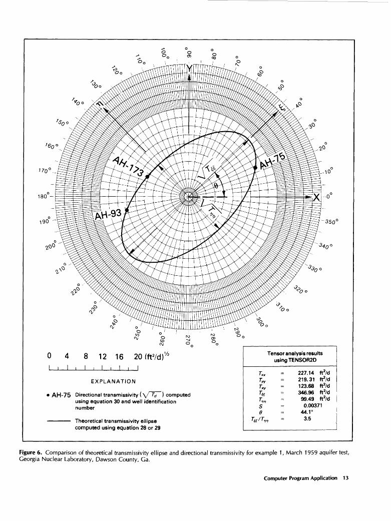
6. Graph showing comparison of theoretical transmissivity ellipse and directional transmissivity for example 1, March 1959 aquifer test, Georgia Nuclear Laboratory, Dawson County, Ga. 13
7. Graph showing comparison of least-squares transmissivity ellipse and directional transmissivity for example 2, March 1959 aquifer test, Georgia Nuclear Laboratory, Dawson County, Ga. 14
8. Graph showing comparison of weighted least-squares transmissivity ellipse and di rectional transmissivity for example 3, March 1959 aquifer test, Georgia Nuclear Laboratory, Dawson County, Ga. 15
Contents III
TABLES
1. Cartesian coordinates and curve matching values for observation wells used in ex ample 1 12
2. Cartesian coordinates and curve matching values for observation wells used in ex amples 2 and 3 12
METRIC CONVERSION FACTORSFor those readers who may prefer to use metric units rather than the inch-pound unit, the conversion factors for the terms used in this
report are listed below:
Multiply inch-pound By To obtain metric unit
LENGTH
inch (in.) foot (ft) mile (mi)
25.40 .3048
1.609
millimeter (mm) meter (m) kilometer (km)
AREA
square mile (mi2) 2.590 square kilometer (km2)
VOLUME
gallon (gal) 3.785 X 10' 3 3.785
cubic meter (m3) liter (L)
FLOW
gallon per minute (gal/min)
6.309 x 10~ 3
0.06309
cubic meter per second (m3/s)
liter per second (L/s)
TRANSMISSIVITY
foot squared per day (ft2/d)
0.09290 meter squared per day(m2/d)
IV Contents
Methods and Computer Program Documentation for Determining Anisotropic Transmissivity Tensor Components of Two-Dimensional Ground-Water Flow
By Morris L. Maslia and Robert B. Randolph
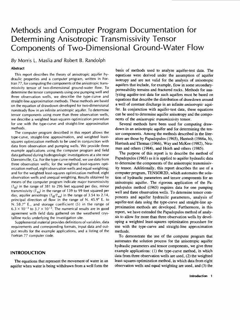
Abstract
This report describes the theory of anisotropic aquifer hy draulic properties and a computer program, written in For tran 77, for computing the components of the anisotropic trans- missivity tensor of two-dimensional ground-water flow. To determine the tensor components using one pumping well and three observation wells, we describe the type-curve and straight-line approximation methods. These methods are based on the equation of drawdown developed for two-dimensional nonsteady flow in an infinite anisotropic aquifer. To determine tensor components using more than three observation wells, we describe a weighted least-squares optimization procedure for use with the type-curve and straight-line approximation methods.
The computer program described in this report allows the type-curve, straight-line approximation, and weighted least- squares optimization methods to be used in conjunction with data from observation and pumping wells. We provide three example applications using the computer program and field data gathered during hydrogeologic investigations at a site near Dawsonville, Ga. For the type-curve method, we use data from three observation wells; for the weighted least-squares opti mization method, eight observation wells and equal weighting; and for the weighted least-squares optimization method, eight observation wells and unequal weighting. Results obtained by means of the computer program indicate major transmissivity (T^) in the range of 381 to 296 feet squared per day, minor transmissivity (T^) in the range of 139 to 99 feet squared per day, aquifer anisotropy (T^T^) in the range of 3.54 to 2.14, principal direction of flow in the range of N. 45.9° E. to N.58.70 E., and storage coefficient (S) in the range of 6.3 x 10~ 3 to 3.7 x 1CT 3 . The numerical results are in good agreement with field data gathered on the weathered crys talline rocks underlying the investigation site.
Supplemental material provides definitions of variables, data requirements and corresponding formats, input data and out put results for the example applications, and a listing of the Fortran 77 computer code.
INTRODUCTION
The equations that represent the movement of water in an aquifer when water is being withdrawn from a well form the
basis of methods used to analyze aquifer-test data. The equations were derived under the assumption of aquifer isotropy and are not valid for the analysis of anisotropic aquifers that include, for example, flow in some secondary- permeability terrains and fractured rocks. Methods for ana lyzing aquifer-test data for such aquifers must be based on equations that describe the distribution of drawdown around a well of constant discharge in an infinite anisotropic aqui fer. In conjunction with aquifer-test data, these equations can be used to determine aquifer anisotropy and the compo nents of the anisotropic transmissivity tensor.
Several methods have been used for computing draw down in an anisotropic aquifer and for determining the ten sor components. Among the methods described in the liter ature are those by Papadopulos (1965), Hantush (1966a, b), Hantush and Thomas (1966), Way and McKee (1982), Neu- man and others (1984), and Hsieh and others (1985).
The purpose of this report is to describe the method of Papadopulos (1965) as it is applied to aquifer hydraulic data to determine the components of the anisotropic transmissiv ity tensor. Additionally, this report describes the use of a computer program, TENSOR2D, which automates the solu tion of hydraulic parameters and tensor components for an anisotropic aquifer. The rigorous application of the Pa padopulos method (1965) requires data for one pumping well and three observation wells. To determine tensor com ponents and aquifer hydraulic parameters, analysis of aquifer-test data using the type-curve and straight-line ap proximation methods are developed. Furthermore, in this report, we have extended the Papadopulos method of analy sis to allow for more than three observation wells by devel oping a weighted least-squares optimization procedure for use with the type-curve and straight-line approximation methods.
To demonstrate the use of the computer program that automates the solution process for the anisotropic aquifer hydraulic parameters and tensor components, we give three example applications: (1) the type-curve method, in which data from three observation wells are used, (2) the weighted least-squares optimization method, in which data from eight observation wells and equal weighting are used, and (3) the
Introduction 1
weighted least-squares optimization method, in which data from eight observation wells and unequal weighting are used. The data for these example applications were obtained during hydrogeologic investigations at a site near Daw- sonville, Ga. (Stewart, 1964; Stewart and others, 1964).
The work and computer simulation presented in this re port were done in cooperation with the city of Brunswick and Glynn County, Ga.
THEORY OF ANISOTROPIC AQUIFER HYDRAULIC PROPERTIES
A porous medium is considered to be isotropic if all significant properties of the medium are independent of direction (Lohman and others, 1972, p. 9). If, however, at an arbitrary point in the medium the properties vary with direction, the medium at that point is referred to as an isotropic (Bear, 1972, p. 134). In considering two- dimensional ground-water flow, we see that some aquifers are anisotropic. For example, in carbonate rock aquifers, flowing ground water dissolves the rocks, producing solu tion channels primarily along the direction of flow. The rocks then become anisotropic making the aquifer more permeable along the solution channels.
In an anisotropic aquifer, T is defined as a second-rank tensor quantity of transmissivity (Bear, 1972, p. 137; Bear, 1979, p. 72). It is a linear transformation relating hydraulic gradient, / (in the downstream direction), to the discharge, 2*, averaged over the thickness of the aquifer per unit width normal to the flow direction (fig. 1). T can be represented with respect to an arbitrary set of orthogonal axes (x-y) by a 2x2 matrix, such that
(Dyy
Because the transmissivity tensor is symmetric (Bear, 1979, p. 72), Txy =Tyx . Additionally, the determinant, D ', of T is defined as
(2)
In an anisotropic aquifer, the hydraulic gradient, /, and discharge, q*, are not necessarily in the same direction (fig. 1A). However, in certain directions, termed the princi pal directions, / and q* are parallel (fig. IB). These princi pal directions correspond to greatest and least-preferred flow directions. In these directions, the ratio between q* and J is known as the principal value of the transmissivity tensor or principal transmissivity. Because the principal val ues are all distinct, these principal directions are mutually orthogonal and can be used to define the principal coordi nate system. For the principal ^,-r\ coordinate system, T has the form
(3)
where Tg and T^ are defined as the major and minor or principal components of transmissivity, respectively.
The distribution of drawdown around a fully penetrating well of constant discharge in an infinite, anisotropic, con fined aquifer is described by the following equation (Pa- padopulos, 1965, p. 22):
subject to the following initial and boundary conditions:
s(x,y,Q)=Q (5)
s(±<*>,y,t)=Q (6)
s(x, ±oo ( f)=0 , (7)
where 5= the drawdown, (L),T^, Tyy, Txy components of the anisotropic trans
missivity tensor, (L 2/T),S= storage coefficient, (L°),0 =discharge of the well, (L 3/T)/(L 2 of aquifer),8=Dirac delta function,x,y = coordinates of an arbitrary set of orthogonal
axes with the origin at the discharge well, (L), andt =time since pumping started, (T).
Under the assumption of aquifer homogeneity, 7^, T^,, and Tjy are assumed to be constant over the contributing volume of the aquifer under consideration.
We can solve the problem by using and applying initial- condition equation 5 and the Laplace transformation with respect to time (t} to solve equation 4. Then the complex Fourier transform with respect to jc and y is applied with boundary condition equations 6 and 7. The formal solution to equation 4 given by Papadopulos (1965) is
47TVD 7
(8)
where W^w^), known as the Theis well function, is defined as:
METHODS FOR DETERMINING ANISOTROPIC Type-Curve TRANSMISSIVITY TENSOR COMPONENTS
In an anisotropic aquifer, the drawdown caused by pump ing is directionally dependent that is, it is not radially symmetric. Therefore, during an aquifer test, the drawdown at each observation well must be analyzed, and a plot of observed drawdown (5) versus time (t or lit} must be made. Either the type-curve (Theis, 1935) or the straight-line method (Cooper and Jacob, 1946; Jacob, 1950) can be used to analyze the observation-well data. In order to compute the tensor components and the anisotropic aquifer parameter values, one must first determine the four constants in equa tion 10 (T^, Tyy, T^, and 5). Therefore, one pumping well located at the origin of an arbitrary Cartesian coordinate system and a minimum of three observation wells are re quired (fig. 2). Although the distribution of the wells around the pumping well is arbitrary as long as no two observation wells are radially aligned with the pumping well, the degree of radial distribution of observation wells tends to influence the results of the tensor analysis.
For each observation well, a log-log plot of observed drawdown versus time (or inverse time) is graphically (or numerically) matched with the Theis type-curve resulting in match-point values ofs*,t*,W(u)*, and u * for each of the three observation wells. The drawdown (5*), well function (W(u)*), and the flow rate of the pumping well (Q) are then substituted into equation 8 to solve for the determinant (D ') for each set of observation-well data as follows:
(11)
D' should have approximately the same value for each ob servation well. If not, an average value should be selected. Rearranging equation 10 results in
STxx (y 2)+STyy (x 2)-2STxy (Xy)=4tuxyD' . (12)
Replacing values of u^ , x, and y for each observation well
(J)
B
EXPLANATION
Microscopic flow-path of water particle
Ground-water discharge
Hydraulic gradient in the downstream direction
Figure 1. Relationships between the hydraulic gradient (/) and discharge (q*) in an anisotropic aquifer. A, Hydraulic gradient (/) and discharge (q*) aligned along different directions in an anisotropic aquifer. B, Hydraulic gradient (/) and discharge (q*) are parallel and aligned along the principal directions in an anisotropic aquifer.
Methods for Determining Components 3
and D' from equation 11 results in a system of three simul taneous equations of the general form
AX=B ,
where
y\
~Y -- -
(13)
, andS7V
(15)
n _ (16)
(14) In equation 14, xf and yt (i = l, 2, 3) are the coordinate values of the three observation wells with respect to the
OW-2
OW-3
Y
OW-1
A ^ X
Figure 2. Arbitrary Cartesian coordinate system aligned with reference to the pumping well (PW-1) and observation wells OW-1 OW-2, and OW-3.
arbitrary Cartesian coordinate system shown in figure 2. The values of (w*), (7 = 1, 2, 3) in equation 16, are deter mined from the Theis curve match for each observation well, and D' is the determinant derived from equation 11.
Equation 13 can be solved by any number of simultaneous equation solvers. In this report, LU decomposition by the Crout method is used (Stewart, 1973). In the code listing ("Supplemental Data IV"), IMSL 1 routines LUDATF and LUELMF are used to solve equation 13. Upon solving equa tion 13, we obtain values for ST^, STyy , and ST^.
Multiplying both sides of equation 2 by S 2,and rearrang ing, yields
(17)
The storage coefficient for the anisotropic system is then obtained by solving equation 17
values of the transmissivity tensor, which can be expressed as
D'
where ST^ , STyy , ST^ are obtained by solving the system of equations 13, and D' is the determinant derived from equa tion 11. Using the computed value of S from equation 18 and the three values previously obtained from equation 13, we can determine the components of T, such that
i/5 (19)
i/5 (20)
i/5 . (21)
To determine the principal values of T, we solve the eigenvalue problem
TX=XX (22)
by substituting for the components of T and rearranging
r«-x TX(23)
Setting the determinant of the matrix in equation 23 to zero, multiplying, and rearranging result in
\2 -\(TXX +Tyy)+TXXTyy-Txy 2 =Q , (24)
which is a quadratic equation. Because T is symmetric, there will be two real roots. These roots are the principal
(25)
(26)
Aquifer anisotropy is now defined as the ratio T^T^. The angle (6) between the x-axis and the maximum principal direction can be found as follows:
(27)
Using the computed principal values, we determine the equation of the theoretical transmissivity ellipse as
(28)
(18) where £,T]=the axes of the principal coordinate systemrotated by 6 degrees from the arbitrary x-y coordinate system,
=the major axis of the transmissivity ellipse, and
= the minor axis of the transmissivity ellipse.
We can graphically determine the components of the trans missivity tensor by plotting equation 28 on polar-coordinate paper (fig. 3). Alternatively, using the equation by Hantush and Thomas (1966)
(29)
where rp =the theoretical directional transmissivity, and
P=the direction of Tp from the origin with respect to the £-7] coordinate system,
we can obtain the transmissivity ellipse by plotting vTp in the direction of p on polar-coordinate paper (fig. 3).
We can calculate the directional transmissivity with re spect to flow using data from each observation well by (Hantush, 1966b, p. 422)
Sr2
'Use of brand/trade names in this report is for identification purposes only and does not constitute endorsement by the U.S. Geological Survey.
(30)
where Td =the directional transmissivity at the observa tion well,
S =the composite storage coefficient as defined byequation 18,
r =the radial distance from the origin of the arbi trary x-y coordinate system to the observa tion well (fig. 2),
f*=the time at the match point determined by
Methods for Determining Components 5
Theis curve matching at each observation well, and
M* =the variable of the well function at the match point for the observation well.
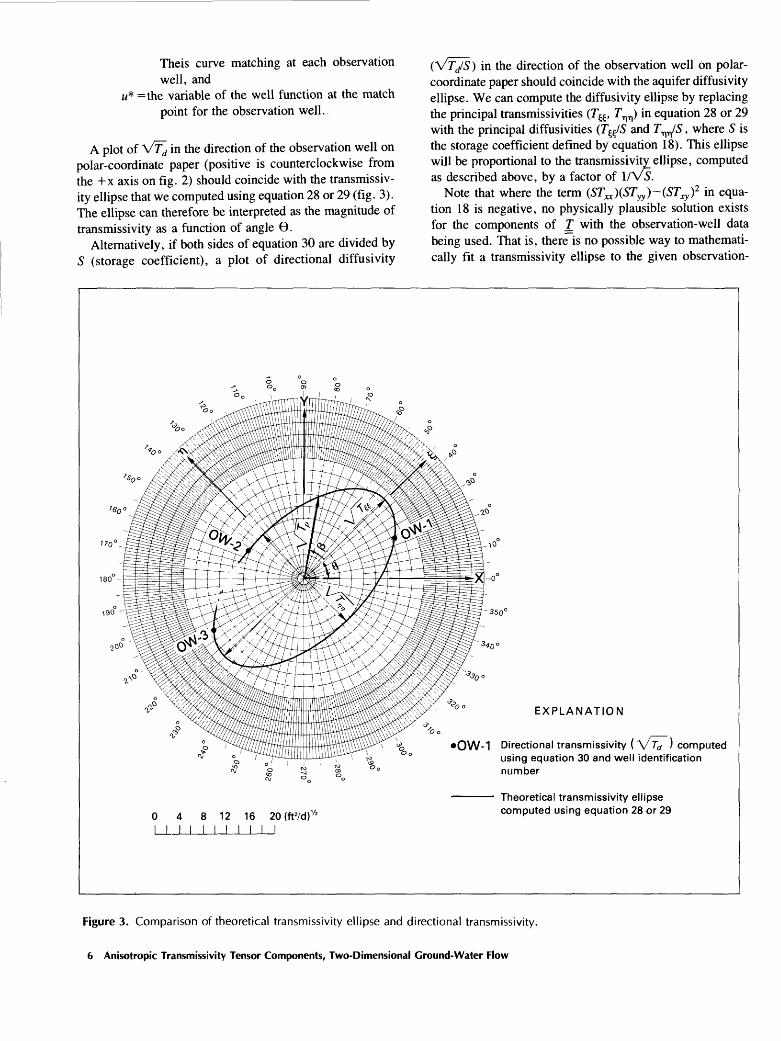
A plot of vYd in the direction of the observation well on polar-coordinate paper (positive is counterclockwise from the +x axis on fig. 2) should coincide with the transmissiv- ity ellipse that we computed using equation 28 or 29 (fig. 3). The ellipse can therefore be interpreted as the magnitude of transmissivity as a function of angle 0.
Alternatively, if both sides of equation 30 are divided by S (storage coefficient), a plot of directional diffusivity
(VjyS) in the direction of the observation well on polar- coordinate paper should coincide with the aquifer diffusivity ellipse. We can compute the diffusivity ellipse by replacing the principal transmissivities (T^, 7^) in equation 28 or 29 with the principal diffusivities (T^S and T^/S, where 5 is the storage coefficient defined by equation 18). This ellipse will be proportional to the transmissivity ellipse, computed as described above, by a factor of I/VS.
Note that where the term (STxx )(STyy )-(STxy )2 in equa tion 18 is negative, no physically plausible solution exists for the components of T with the observation-well data being used. That is, there is no possible way to mathemati cally fit a transmissivity ellipse to the given observation-
-350°
EXPLANATION
OW-1 Directional transmissivity ( \Td ) computed using equation 30 and well identification number
0 4 8 12 16 20(ft2/d) 1/2I I I I I I I I I I I
Theoretical transmissivity ellipse computed using equation 28 or 29
Figure 3. Comparison of theoretical transmissivity ellipse and directional transmissivity.
well data. A plot of VT/S in the direction of the observa tion wells on polar-coordinate paper should indicate that the data are scattered, and it is not possible to fit a single ellipse through the three points. This may indicate that the field data are in error, the assumption of aquifer homogeneity is incorrect, the aquifer cannot be conceptualized as an an- isotropic porous medium, or the quantity and distribution of observation wells are insufficient to describe the flow regime of the aquifer.
Straight-Line Approximation
For small values of u (w<0.01), equation 9 can be ap proximated (Cooper and Jacob, 1946; Jacob, 1950) such that
logio (31)
Substituting equations 31 and 10 into equation 8 yields
D'2.3030 , (2.25t ~ log 10 -(32)
For each of the three observation wells, plot drawdown (s) versus time (t ) on semilog graph paper with t on the loga rithmic axis; equation 32 plots as a straight line with
m2.3030 , = 7=== , and
=-M:1 2.25 L D'
(33)
(34)
where ra=the slope of the line defined by equation 32,which is As per log cycle, and
t0 =the intercept of the straight line with the time axis when s=Q.
Rearranging equations 33 and 34 yields
,2_, f2.303(2 r A D = 4 -\ , andJ
STxx (y 2)+STyy (x 2)-2STxy (xy)=2.25t0D' .
(35)
(36)
The slope of the drawdown versus time data for each observation well should be approximately the same, thereby giving the same value for D ' for each well (as previously discussed). By substituting the computed value of D' from equation 35 into equation 36, we can write a linear system of three simultaneous equations in the same form described by equation 13. A and X are defined by equations 14 and 15, respectively, and B has the form
{2.25(1^0''8=12.25(1^0'
[2.25(tQ)3D'(37)
in which (?0X (/ = 1, 2, 3) is the intercept of the straight line with the t axis at s =0 for each observation well, and D' is defined by equation 35. We can now solve the system of three simultaneous equations (equation 13) by using the methods previously described. We can also compute com ponents of T, the principal values of T, and the principal direction of anisotropy by following the procedures de scribed in equations 17 through 27.
We can compute the directional transmissivity (Td ) using the straight-line data for each observation well by substitut ing for u* in equation 30 (by using equation 10) and simpli fying such that
-2D'
(38)
Rearranging equation 34 yields
D'
2.25f0
and substituting equation 39 into equation 38 results in
Sr 2
(39)
T (40)
As previously discussed, a plot of V?^ in the direction of each observation well on polar-coordinate paper should co incide with the transmissivity ellipse, which we computed using equation 28 or 29, and will be proportional to a plot of VTjS by a factor of l/Vs.
Least-Squares Optimization
The assumption of aquifer homogeneity is not always valid in field situations. Where significant heterogeneity occurs, the use of three observation wells in different direc tions to define the principal transmissivities will not always yield a physically plausible solution ((STxx )(STyy )-(STxy )2 in equation 18 can be negative). For example, one of the wells could be drilled into a local fracture that is not repre sentative of the aquifer penetrated by other wells. There fore, one may need more than three observation wells to obtain additional information on the directional characteris tics of ground-water flow at the test site. When more than three observation wells are used, the same type-curve and straight-line procedures described previously can be used. However, equation 13 will have the form
Methods for Determining Components 7
"v? *y\ xy\ x
-2x ly l
~
STy
STr(41)
for the type-curve method, and
2 2 _ *"> CT1 V3 X-$ ZA"3^y3 »JJ Y
yN XN -ZxNyN
for the straight-line method.
'2.25(^,0'
2.25(t0)2D'
2.25(t0)ND'
Equations 41 and 42 represent a linear system of N simul taneous algebraic equations (N is the total number of obser vation wells) with three unknowns (5Txr , Srvv , and ST^). Because the system is over-determined (there are more equations than unknowns), the use of a least-squares opti mization procedure is required to solve the system of equa tions 41 and 42, which are represented by the system of equations 13. Two least-squares procedures may be used to solve the system of equations represented by equation 1 3 the ordinary least-squares (OLS) method and weighted least-squares (WLS) method.
Using the OLS method, we compute the solution to equa tion 13 according to Stewart (1973, p. 221)
A TB (43)
As long as the deviation of V^T~d or Vr/S from the ellipse computed by means of the OLS method is only slight, this method works well. (See, for example, Randolph and others, 1985, fig. 7.)
If the test site is characterized by extreme heterogeneity such that the data being analyzed show large deviations, a physically plausible solution may still fail to exist ((ST^) (STyy ) (STxy )2 in equation 18 is negative). Additionally, if observation-well data is lacking in a certain area (or quad rant) (observation wells are clustered about a certain area or quadrant), equation 43 may yield an ellipse that is unrealis- tically elongated in the direction of the missing data. An other problem that arises in using the OLS method is that elements of B in equation 43 are inversely proportional to directional transmissivity (compare equations 30 and 41). Therefore, the OLS method is more sensitive to smaller values of directional transmissivity. If the data set being considered has significant variations in the values of Td, the ellipse computed from equation 43 will be biased toward the
smaller Td values. Hsieh and others (1985, p. 1670) also noted and discussed these difficulties arising from the use of the OLS method in analyzing well data in three dimensions for computing components of the hydraulic conductivity tensor.
To address the problems associated with the OLS method, we can use an alternative solution methodology, the weighted least-squares method (WLS). Where the WLS method is used, the solution to equation 13 is computed according to Draper and Smith (1981, p. 109) and Beck and Arnold (1977, p. 248):
(44)
where <o is an NX N diagonal matrix of selected weights or coefficients. The elements <o are assigned values so that large values of Td are given appropriate weighting in deriv ing the least-squares transmissivity ellipse and a physically plausible solution to equation 18 exists ((STxx )(STyy )- (STfy)2 is positive). Obviously, the manner in which the values for elements of w are chosen is subjective. As such, one may be required to make several attempts using differ ent weights to obtain an acceptable solution if the data show a large degree of scatter.
Situations may arise (1) where the scatter of the data is so large that a fit of the field data (Vf~d or Vr/S) to a com puted ellipse is not possible even with the use of the WLS method and a judicious choice of weights or (2) where s * and t* data show a lack of fit to the type curve (or straight line). When either of these situations occurs, the aquifer being tested cannot be represented as an anisotropic, homo geneous porous medium on the scale of the aquifer volume being tested. If the aquifer being tested is sufficiently homo geneous so that the methods described herein can be gener ally applied (a plot of V^f~d or \/TdIS in the direction of the observation wells outlines an ellipse similar to the one derived from equation 43 or 44), then every possible combi nation of any of the three observation wells in three different directions should yield approximately the same results.
COMPUTER PROGRAM DESCRIPTION
The computer code listing presented in this report ("Supplemental Data V") is written in Fortran 77 and is intended for use on the PRIME computer system of the U.S. Geological Survey, Water Resources Division. The pro gram, TENSOR2D, is composed of a main program and four subroutine subprograms. A generalized flow chart of TENSOR2D is shown in figure 4. The purpose of the main program and each subroutine is explained below: MAIN PROGRAM: Dimensions the appropriate arrays and
allocates the space in storage vector Y. At the present time, enough space is allocated in Y to analyze 25 observation wells. If more space is required, increase the size of Y.
Figure 4. Generalized flow chart of the computer program.
Computer Program Description 9
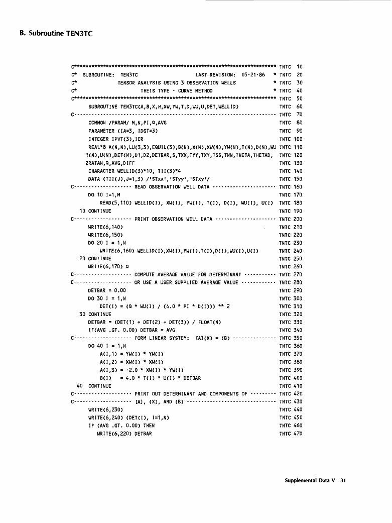
SUBROUTINE TEN3TC: Uses the results of the type- curve method to compute tensor components and aqui fer anisotropy for three observation wells. The system of simultaneous equations is solved by LU decomposi tion using the Crout method.
SUBROUTINE TEN3SL: Uses the results of the straight- line method to compute tensor components and aquifer anisotropy for three observation wells. The system of simultaneous equations is solved by LU decomposition using the Crout method.
SUBROUTINE WLSTC: Uses the results of the type-curve method to compute tensor components and aquifer an isotropy for four or more observation wells. The sys tem of simultaneous equations is solved by a weighted least-squares optimization scheme.
SUBROUTINE WLSSL: Uses the results of the straight- line method to compute tensor components and aquifer anisotropy for four or more observation wells. The system of simultaneous equations is solved by a weighted least-squares optimization scheme.
The definitions of selected variables used in TENSOR2D are listed in "Supplemental Data I," and formats of required input data are listed in "Supplemental Data II." TENSOR2D is written in a modular form to accommodate user modifica tion of input data and output results. Additionally, all input data must be in consistent units.
COMPUTER PROGRAM APPLICATION
Three numerical examples are provided to demonstrate the use of TENSOR2D. In example 1, the type-curve method is used for analyzing data from three observation wells. Examples 2 and 3 show the type-curve method used with data from eight observation wells (weighted least- squares method). In example 2, the elements of the weight matrix ( o> in equation 44) are all assigned a value of unity (1.0). This is the same as using the ordinary least-squares method (equation 43). In example 3, the weights assigned to to are varied in order to demonstrate the effect of weighting on the computedtransmissivity ellipse.
Data used in the examples were gathered during hydroge- ologic investigations at the site of the Georgia Nuclear Lab oratory, about 4 miles southwest of Dawsonville, Dawson County, Ga., and reported in Stewart (1964) and Stew art and others (1964). Data used in the example problems are listed in tables 1 and 2. Required input data in TENSOR2D format and solutions of the example problems are given in "Supplemental Data III" and "IV," respectively.
Example 1. Type-Curve Method Three Observation Wells
On March 17-19, 1959, an aquifer test was conducted at the site of the Georgia Nuclear Laboratory to determine the capacity of saprolite, which underlies the test site, to trans
mit water and to yield water from storage. The estimated saturated thickness of the saprolite at the test site is about 100 feet (Stewart, 1964, p. D51). Discharge from the pump ing well (TW-16) was 8.7 gallons per minute for about 30 hours. The location of observation wells AH-75, AH-93, and AH-173 and the arbitrary Cartesian (x-y) coordinate system used for the tensor analysis are shown in figure 5. All time-drawdown data were matched with the Theis type curve. Coordinate values, radial distances and direction from the pumping well (TW-16), and type-curve match- point values for the three observation wells are listed in table 1.
The arbitrary coordinate system was oriented with the y- axis to the north (fig. 5). As previously discussed, D' (equation 11) should have the same value for each obser vation well. In this example (and most field situations), D' varies somewhat for each observation well (table 1). There fore, an arithmetic average of 3.452X 10⁴ (ft2/d)2 was used forD' in the tensor analysis. TENSOR2D will calculate an average D' using all the observation wells, or the user can specify a D' of his choosing. (See "Supplemental Data II" and "IV.")
Components of the transmissivity tensor and the storage coefficient computed by TENSOR2D, a plot of the trans missivity ellipse, and the directional transmissivity for each observation well are shown in figure 6. The values com puted for the directional diffusivity (TJS} are also listed in table 1. The plot of V/;J (equation 30 and table 1) in the direction of the observation well (fig. 6) coincides exactly with the theoretical transmissivity ellipse (computed using equation 28 or 29) because only three observation wells were used. The angle of anisotropy and principal direction of flow computed by TENSOR2D (6-44.1°; N. 45.9° E.) are in good agreement with the alignment of the major axis of the observed cone of depression defined during a June 1958 aquifer test (Stewart and others, 1964, pi. 3). The azimuth of the major axis of this cone is about N. 52° E. and is parallel to the strike of rock foliation in the area of the aquifer test (Stewart and others, 1964, p. F68). The output from example 1 is provided in "Supplemental Data IV."
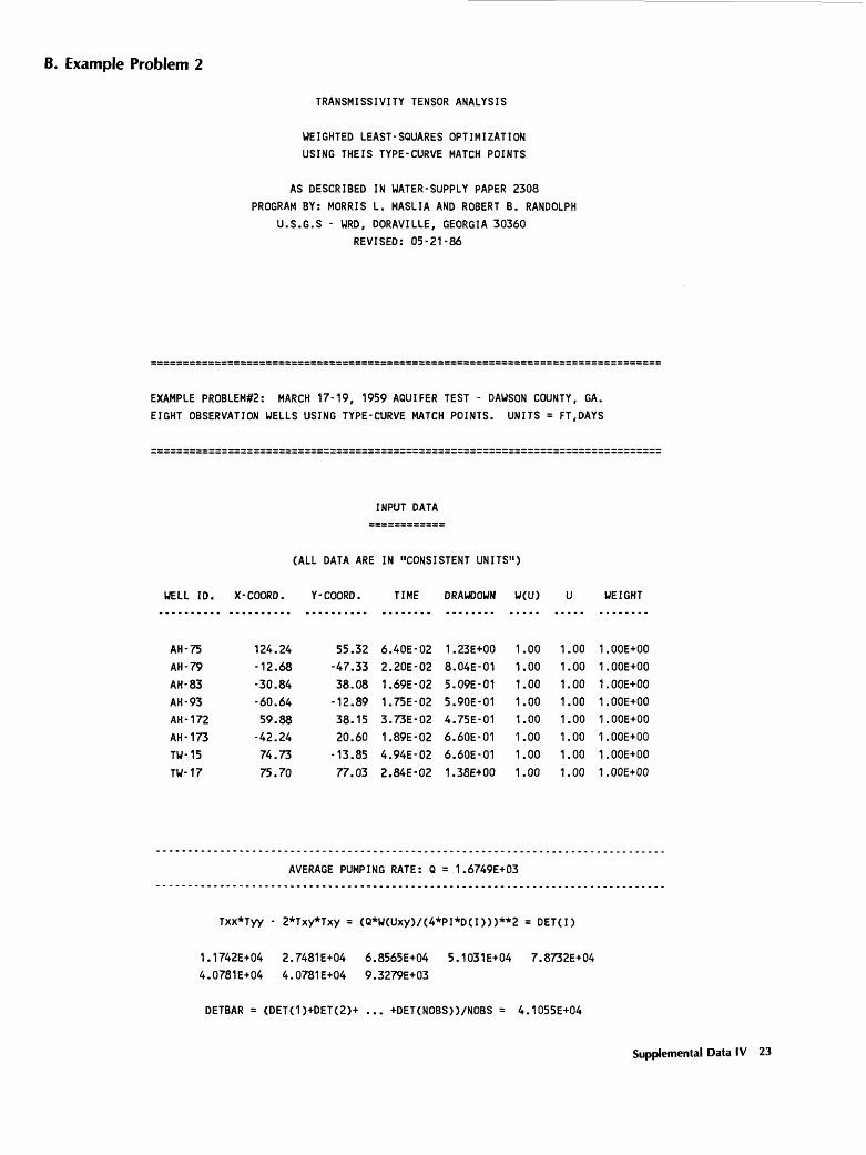
Example 2. Type-Curve Method and Equal Weighted Least-Squares Optimization Eight Observation Wells
In this example, we computed components of the trans missivity tensor and the storage coefficient using the eight observation wells shown on figure 5, and data relative to the same aquifer test described in example 1. Table 2 lists coordinate values, radial distances and direction of the ob servation wells from the pumping well (TW-16), type- curve match points, and values of D' (computed using equa tion 11). As with example 1, the value of D' varied for each observation well (table 2), so TENSOR2D computed an arithmetic average for use in the tensor analysis. (See output
of example 2 in "Supplemental Data IV.") Because there were more than three observation wells, the weighted least- squares method was used to solve the over-determined sys tem of equations (subroutine WLSTC of TENSOR2D in fig. 4 and "Supplemental Data V"). In this example, the weights (to in equation 44) were all assigned a value of 1.0 ("Supplemental Data II" and "III"). A justification of these values would be that test data from each observation well are considered to be of equal quality and did not show signifi cant scatter.
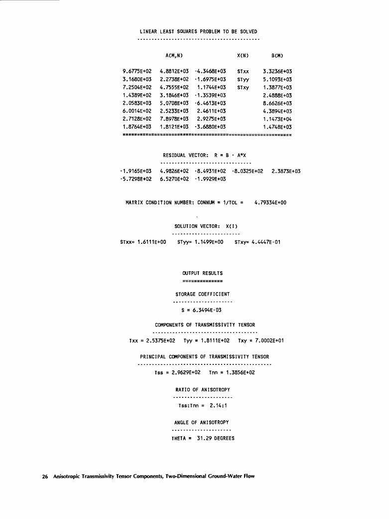
Results of the tensor analysis are shown on figure 7. The Vr~d (equation 30) for each observation well (Td/S is listed in table 2) plotted in the direction of the observation well, compares favorably with and outlines the least-squares transmissivity ellipse computed using equation 28 or 29
(fig. 7). Additionally, the ratio of anisotropy (3.5:1) and angle of anistropy (0=43.4°, N. 46.6° E.) agree well with results from example 1 and the field observations reported in Stewart and others (1964, pi. 3).
The close agreement between results of example 1 (three observation wells) and example 2 (eight observation wells) is one indication that the assumption of aquifer homogeneity is valid for these field data. Another indication that the assumption of a homogeneous porous medium is correct is apparent in the equal weights assigned to the observation- well data ( to in equation 44 and WT(I) in "Supplemental Data III-B" and "IV-B"). Because all observation wells were equally weighted (assigned a value of 1.0) and the square root of the directional transmissivity 0/7^) for the wells aligned closely with the computed transmissivity el-
AH-173
AH-93 V
AH-79
TW-17
N
' i
AH-75
50 100 I
150 FEET
10 20 30I
40 METERS
Figure 5. Location of pumping well (TW-16), observation wells, and arbitrary x-y coordinate system used in the analysis of the March 1959 aquifer test, Georgia Nuclear Laboratory, Dawson County, Ga.
Computer Program Application 11
lipse, the assumption of aquifer homogeneity appears to be valid. If the test data had shown significant scatter, indicat ing possible aquifer heterogeneities, we may have had to assign different weighting values to the observation wells in order to compute the tensor components and anisotropic aquifer parameter values.
Example 3. Type-Curve Method and Unequal Weighted Least-Squares Optimization Eight Observation Wells
Example 3 is provided to demonstrate the effect of assign ing different values of weight ( w in equation 44) to the test data on the computed transmissivity ellipse and components of the transmissivity tensor. All input data are the same as those in example 2 (table 2), with the exception of the weighting values (compare "Supplemental Data III B" and "III-C"). Wells AH-79, AH-172, AH-173, and TW-15 (fig. 5) were arbitrarily assigned a weight of 2.0, whereas wells AH-75, AH-83, AH-93, and TW-17 were assigned weights of 0.1, 0.25, 0.75, and 0.1, respectively. This implies that during the solution process of equation 44,
wells AH-75 and TW-17 will be given the least amount of weight, whereas wells AH-79, AH-172, AH-173, and TW-15 will be weighted the most. It should be noted again that these weights were assigned arbitrarily to demonstrate the effect of using the weighted least-squares method.
Results of the tensor analysis using the weighting distri bution described above are shown on figure 8. A plot of vT~d (equation 30) for each observation well (TdIS is listed in table 2) in the direction of the well shows that the wells that were weighted the most (AH-79, AH-172, AH-173, and TW-15) align most closely with the computed trans missivity ellipse. Additionally, the ratio of anisotropy has been reduced from 3.5:1 (example 2) to 2.1:1. Computed values of the tensor components, the angle of anisotropy, and the storage coefficient are also shown in figure 8.
An important point demonstrated by example 3 is that the weighted least-squares method allows one to use subjective judgment in evaluating the quality of data from the observa tion wells. Additionally, if some heterogeneities are present at the test site, they can be taken into account by the assign ment of different weights ( w in equation 44) during the solution procedure.
Table 1. Cartesian coordinates and curve matching values for observation wells used in example 1
Well identification
4AH-75
AH-93 AH-173
X
(ft)
124.24 -60.64 -42.24
Y (ft)
55.32 -12.89
20.60
r (ft)
136 6247
Type-curve match points
(degrees)
24° 192° 154°
W(u)
1.0 1.0 1.0
u
1.0 1.0 1.0
s (ft)
1.23 .59 .66
t (days)
0.0640 .0175 .0189
D'2(ft2/d)2
1.174X10⁴ 5.103X10⁴ 4.078X104
V* 3 (ft2/d)
7.23X10⁴ 5.49X10⁴ 2.92X10⁴
'Direction of observation well; positive is counterclockwise from +x axis.2See equation 11 for definition of D'.3See equation 30 for definition of Td. Computed value of 5 in example 1=3.71 x 10~ 3 .4See figure 5 for well locations.
Table 2. Cartesian coordinates and curve matching values for observation wells used in examples 2 and 3
'Direction of observation well; positive is counterclockwise from +x axis.2See equation 11 for definition of D'.3See equation 30 for definition of Td. Computed value of 5 in example 2=4.38X 10~ 3 . Computed value of 5 in example 3=6.35X 10~ 3 .4See figure 5 for well locations.
Figure 6. Comparison of theoretical transmissivity ellipse and directional transmissivity for example 1, March 1959 aquifer test, Georgia Nuclear Laboratory, Dawson County, Ga.
Computer Program Application 13
Oo <0
"Oo
'3.
180
<V
0 4 8 12 16 20(ft2/d) /2I I I I I I I I I I I
EXPLANATION
AH-75 Directional transmissivity (\/ Ta ' computed using equation 30 and well identification number
Theoretical transmissivity ellipse computed using equation 28 or 29
Figure 7. Comparison of least-squares transmissivity ellipse and directional transmissivity for example 2, March 1959 aquifer test, Georgia Nuclear Laboratory, Dawson County, Ga.
AH-75 Directional transmissivity \\/ Td I computed using equation 30 and well identification number
Theoretical transmissivity ellipse computed using equation 28 or 29
Tensor analysis results using TENSOR2D
Tee
JVYTyy
xy
T«'TJTJ
sefa
253.75181.1170.00
296.29138.56
ft2/dft2/dft2/dft2/dft2/d
0.0063531.3°
2.1
Figure 8. Comparison of a weighted least-squares transmissivity ellipse and directional transmissivity for example 3, March 1959 aquifer test, Georgia Nuclear Laboratory, Dawson County, Ga.
Computer Program Application 15
SUMMARY
The computer program, TENSOR2D, described in this report can be used to compute the anisotropic aquifer hy draulic parameters and components of the transmissivity tensor for two-dimensional ground-water flow. The pro gram is based on the equation of drawdown formulated by Papadopulos (1965) for nonsteady flow in an infinite an isotropic aquifer. Using aquifer-test data for one pumping well and three observation wells, we have developed the type-curve and straight-line approximation methods for computing anisotropic aquifer hydraulic properties and components of the transmissivity tensor. Additionally, we have extended the method of Papadopulos (1965) as origi nally developed to allow for the analysis of more than three observation wells by applying a weighted least-squares opti mization procedure to the type-curve and straight-line ap proximation methods.
We provided three example applications using the com puter program and field data gathered during hydrogeologic investigations at a site near Dawsonville, Ga. (Stewart, 1964; Stewart and others, 1964),to illustrate the use of the computer program, TENSOR2D: the type-curve method, where data from three observation wells are used; the weighted least-squares optimization method, where eight observation wells and equal weighting are used; and the weighted-least squares optimization method, where eight observation wells and unequal weighting are used. Results obtained by means of the computer program indicate major transmissivity (7^) in the range of 381 to 296 feet squared per day, minor transmissivity (7^) in the range of 139 to 99 feet squared per day, aquifer anisotropy in the range of 3.54 to 2.14, principal direction of flow in the range of N. 45.9° E. to N. 58.7° E., and computed storage coeffi cients in the range of 6.3x 10~3 to 3.7X 10~ 3 . The numeri cal results are in good agreement with the field data gathered on the weathered crystalline rocks underlying the investiga tion site.
The names of program variables, data input formats, ex amples of input data and model output, and the Fortran 77 computer code of TENSOR2D are listed in the "Supple mental Data" sections. The program is written in a modular format to allow user modification of input data and output results.
REFERENCES CITED
Bear, Jacob, 1972, Dynamics of fluids in porous media: New York, American Elsevier Publishing Company, 764 p.
1979, Hydraulics of groundwater: New York, McGraw- Hill, 567 p.
Beck, J.V., and Arnold, K. J., 1977, Parameter estimation in engi neering science: New York, John Wiley, 709 p.
Cooper, H.H., and Jacob, C.E., 1946, A generalized graphical method for evaluating formation constants and summarizing well-field history: American Geophysical Union Transaction, v. 27, no. 4, p. 526-534.
Draper, Norman, and Smith, Harry, 1981, Applied regression analysis: New York, John Wiley, 709 p.
Hantush, M.S., 1966a, Wells in homogeneous anisotropic aquifers: Water Resources Research, v. 2, no. 2, p. 273-279.
1966b, Analysis of data from pumping tests in anisotropic aquifers: Journal of Geophysical Research, v. 71, no. 2, p. 421-426.
Hantush, M.S., and Thomas, R.G., 1966, A method for analyzing a drawdown test in anisotropic aquifers: Water Resources Research, v. 2, no. 2, p. 281-285.
Hsieh, P.A., Neuman, S.P., Stiles, G.K., and Simpson, E.S., 1985, Field determination of three-dimensional hydraulic conductivity tensor of anisotropic media, 2. Methodology and application to fractured rocks: Water Resources Research, v. 21, no. 11, p. 1667-1676.
Jacob, C.E., 1950, Flow of ground water, in Rouse, H., ed., Engineering Hydraulics, chapter 5, New York, John Wiley, Inc., p. 321-386.
Lohman, S.W., and others, 1972, Definitions of selected ground- water terms revisions and conceptual refinements: U.S. Ge ological Survey Water-Supply Paper 1988, 21 p.
Neuman, S.P., Walter, G.R., Bentley, H.W., Ward, J.J., and Gonzalez, D.D., 1984, Determination of horizontal aquifer anisotropy with three wells: Ground Water, v. 22, no. 1, p. 66-72.
Papadopulos, I.S., 1965, Nonsteady flow to a well in an infinite anisotropic aquifer: Proceedings of the Dubrovnik Sympo sium on the Hydrology of Fractured Rocks, International As sociation of Scientific Hydrology, p. 21-31.
Randolph, R.B., Krause, R.E., and Maslia, M.L., 1985, Com parison of aquifer characteristics derived from local and re gional aquifer tests: Ground Water, v. 23, no. 3, p. 309-316.
Stewart, G.W., 1973, Introduction to matrix computations: New York, Academic Press, 441 p.
Stewart, J.W., 1964, Infiltration and permeability of weathered crystalline rocks, Georgia Nuclear Laboratory, Dawson County, Georgia: U.S. Geological Survey Bulletin 1133-D, 59 p.
Stewart, J.W., Callahan, J.T., and Carter, R.F., 1964, Geologic and hydrologic investigation at the site of the Georgia Nuclear Laboratory, Dawson County, Georgia: U.S. Geological Sur vey Bulletin 1133-F, 90 p.
Theis, C. V., 1935, The relation between the lowering of the piezo- metric surface and the rate and duration of discharge of a well using ground-water storage: American Geophysical Union Transactions, v. 16, p. 519-524.
Way, S.C., and McKee, C.R., 1982, In-situ determination of three-dimensional aquifer permeabilities: Ground Water, v. 20, no. 5, p. 594-603.
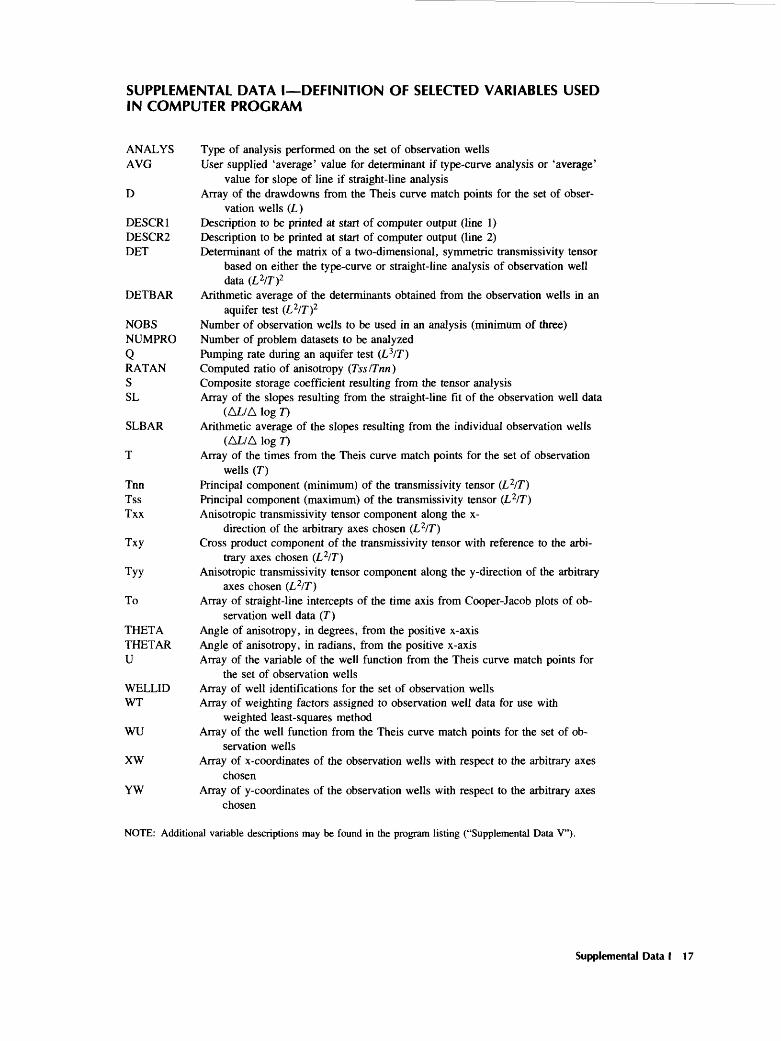
SUPPLEMENTAL DATA I DEFINITION OF SELECTED VARIABLES USED IN COMPUTER PROGRAM
ANALYS Type of analysis performed on the set of observation wellsAVG User supplied 'average' value for determinant if type-curve analysis or 'average'
value for slope of line if straight-line analysisD Array of the drawdowns from the Theis curve match points for the set of obser
vation wells (L)DESCR1 Description to be printed at start of computer output (line 1)DESCR2 Description to be printed at start of computer output (line 2)DET Determinant of the matrix of a two-dimensional, symmetric transmissivity tensor
based on either the type-curve or straight-line analysis of observation well data (L 2/r)2
DETBAR Arithmetic average of the determinants obtained from the observation wells in an aquifer test (L 2/T)2
NOBS Number of observation wells to be used in an analysis (minimum of three)NUMPRO Number of problem datasets to be analyzedQ Pumping rate during an aquifer test (L 3/T)RAT AN Computed ratio of anisotropy (Tss/Tnn)S Composite storage coefficient resulting from the tensor analysisSL Array of the slopes resulting from the straight-line fit of the observation well data
(AL/A log T)SLBAR Arithmetic average of the slopes resulting from the individual observation wells
(AL/A log DT Array of the times from the Theis curve match points for the set of observation
wells (T)Tnn Principal component (minimum) of the transmissivity tensor (L2/T)Tss Principal component (maximum) of the transmissivity tensor (L 2/T)Txx Anisotropic transmissivity tensor component along the x-
direction of the arbitrary axes chosen (L 2/T)Txy Cross product component of the transmissivity tensor with reference to the arbi
trary axes chosen (L 2/T)Tyy Anisotropic transmissivity tensor component along the y-direction of the arbitrary
axes chosen (L2/T)To Array of straight-line intercepts of the time axis from Cooper-Jacob plots of ob
servation well data (T)THETA Angle of anisotropy, in degrees, from the positive x-axisTHETAR Angle of anisotropy, in radians, from the positive x-axisU Array of the variable of the well function from the Theis curve match points for
the set of observation wellsWELLID Array of well identifications for the set of observation wellsWT Array of weighting factors assigned to observation well data for use with
weighted least-squares methodWU Array of the well function from the Theis curve match points for the set of ob
servation wellsXW Array of x-coordinates of the observation wells with respect to the arbitrary axes
chosenYW Array of y-coordinates of the observation wells with respect to the arbitrary axes
chosen
NOTE: Additional variable descriptions may be found in the program listing ("Supplemental Data V").
Supplemental Data I 17
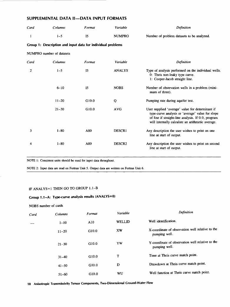
SUPPLEMENTAL DATA II DATA INPUT FORMATS
Card Columns Format Variable
1 1-5 15 NUMPRO
Group 1: Description and input data for individual problems
NUMPRO number of datasets
Card Columns Format Variable
2 1-5 15 ANALYS
6-10
11-20
21-30
1-80
1-80
15
G10.0
G10.0
A80
A80
NOBS
Q
AVG
DESCR1
DESCR2
Definition
Number of problem datasets to be analyzed.
Definition
Type of analysis performed on the individual wells. 0: Theis non-leaky type curve. 1: Cooper-Jacob straight line.
Number of observation wells in a problem (mini mum of three).
Pumping rate during aquifer test.
User supplied 'average' value for determinant if type-curve analysis or 'average' value for slope of line if straight-line analysis. If 0.0, program will internally calculate an arithmetic average.
Any description the user wishes to print on one line at start of output.
Any description the user wishes to print on second line at start of output.
NOTE 1: Consistent units should be used for input data throughout.
NOTE 2: Input data are read on Fortran Unit 5. Output data are written on Fortran Unit 6.
IF ANALYS=1 THEN GO TO GROUP 1.1-B
Group 1.1-A: Type-curve analysis results (ANALYS=0)
NOBS number of cards
Card Columns
I-10
II-20
21-30
31-40
41-50
51-60
Format
A10
G10.0
G10.0
G10.0
G10.0
G10.0
Variable
WELLID
XW
YW
T
D
wu
Definition
Well identification.
X-coordinate of observation well relative to the pumping well.
Y-coordinate of observation well relative to the pumping well.
Variable of the well function at Theis curve match point.
Weight factor for observation well data to be used with weighted least-squares method. For equal weighting set WT=1.0 for all data. WT should be omitted if analyzing only three observation wells.
Group 1.1 -B: Straight-line analysis results (ANALYS=1)
NOBS number of cards
Card Columns Format Variable
1-10 A10 WELLID
11-20 G10.0 XW
21-30
31-40
41-50
51-60
G10.0
G10.0
G10.0
G10.0
YW
To
SL
WT
Definition
Well description.
X-coordinate of observation well relative to the pumping well.
Y-coordinate of observation well relative to the pumping well.
Straight-line intercept of time axis.
Slope of straight line, [(Adrawdown)/(Alog(time))].
Weight factor for observation well data to be used with weighted least-squares method. For equal weighting, set WT=1.0 for all data. WT should be omitted if analyzing only three observation wells.
NOTE 1: Consistent units should be used for input data throughout.
NOTE 2: Input data are read on Fortran Unit 5. Output data are written on Fortran Unit 6.
Supplemental Data II 19
SUPPLEMENTAL DATA III INPUT DATA FOR APPLICATION EXAMPLES
A. Example Problem 1
10 3 1674.8663 0.0
EXAMPLE PROBLEMS: MARCH 17-19, 1959 AQUIFER TEST - DAWSON COUNTY, GA.
EXAMPLE PROBLEM#2: MARCH 17-19, 1959 AQUIFER TEST - DAWSON COUNTY, GA. EIGHT OBSERVATION WELLS USING TYPE-CURVE MATCH POINTS. UNITS = FT,DAYSAH-75AH -79AH -83AH-93AH-172AH-173TU-15TW-17
124.24-12.68-30.84-60.6459.88-42.2474.7375.70
55.32-47.3338.08-12.8938.1520.60-13.8577.03
0.06400.02200.01690.01750.03730.01890.04940.0284
1.2300.8040.5090.5900.4750.6600.6601.380
1.01.01.01.01.01.01.01.0
1.01.01.01.01.01.01.01.0
1.01.01.01.01.01.01.01.0
C. Example Problem 3
10 8 1674.8663 0.0
EXAMPLE PROBLEM#3: MARCH 17-19, 1959 AQUIFER TEST - DAWSON COUNTY, GA.
USE OF DIFFERENT WEIGHTS FOR LEAST-SQUARES. UNITS = FT,DAYS
ANALYS: TYPE OF ANALYSIS PERFORMED ON THE INDIVIDUAL WELLS
0: THEIS NON- LEAKY TYPE CURVE ANALYSIS
1: COOPER- JACOB STRAIGHT LINE ANALYSIS
NOBS: NUMBER OF OBSERVATION WELLS (MINIMUM OF 3)
Q: PUMPING RATE DURING AQUIFER TEST
AVG: USER SUPPLIED 'AVERAGE 1 VALUE FOR DETERMINANT IF TYPE-
CURVE ANALYSIS OR 'AVERAGE 1 VALUE FOR SLOPE OF LINE
IF STRAIGHT-LINE ANALYSIS. IF AVG=0.0 PROGRAM WILL
INTERNALLY CALCULATE AN ARITHMETIC AVERAGEDESCR1: 80 CHARACTER VARIABLE FOR PROBLEM DESCRIPTION
DESCR2: 80 CHARACTER VARIABLE FOR PROBLEM DESCRIPTIONWELLID(I): WELL IDENTIFICATION
XW<I): X- COORDINATE OF WELL
YW(I): Y- COORDINATE OF WELLWT(I): LEAST-SQUARES WEIGHTING COEFFICIENT++++++++++ Data From Theis Type-Curve Match ++++++++++T(I): TIME AT THEIS CURVE MATCH POINT
D(I): DRAWDOWN AT THEIS CURVE MATCH POINT
WU(I): THEIS CURVE MATCH POINT W(U)
U(I): THEIS CURVE MATCH POINT Uxy++++++++++ Data From Cooper-Jacob Straight-Line Match ++++++++++Tod): STRAIGHT LINE INTERCEPT OF TIME AXIS
1 13X,'STxx=',1PEl1.4,2X,'STyy=',E11.4 f 2X, TNSL1410
2 'STxy=',E11.4) TNSL1420
335 FORMAT(//,12X,'**** ERROR: SQUARE ROOT OF NEGATIVE NUMBER **** , TNSL1430
1 /,12X,'* CANNOT COMPUTE STOR. COEFF. OR TRANSM. * , TNSL14402 /,12X,'* WITH GIVEN OBSERVATION WELL DATA *', TNSL14503 / 12X '************************************************') TNSL1460
WRITE(6,170) Q WLSS 320C---.--..----....---- COMPUTE AVERAGE VALUE FOR SLOPE OF LINE --------- WLSS 330
c .................... OR USE A USER SUPPLIED AVERAGE VALUE ------------ WLSS 340
SLBAR =0.00 WLSS 350
DO 30 I = 1,M WLSS 360
SLBAR = SLBAR + SL(I) WLSS 370
WT(I) = DSQRT (WT(I)) WLSS 380
30 CONTINUE WLSS 390
SLBAR = SLBAR / FLOAT(M) WLSS 400
IF(DABS(AVG) .GT. 0.00) SLBAR = AVG WLSS 410c .................... COMPUTE DETERMINANT AND FORM -------------------- WLSS 420
C--.................. LINEAR SYSTEM: [A](X) = (B) .................... WLSS 430
DET = (2.3025851 * Q / (4.0 * PI * SLBAR)) ** 2 WLSS 440
DO 40 I = 1,M WLSS 450
A(I,1) = YW(I) * YW(I) * WT(I) WLSS 460
A(I,2) = XW(I) * XW(I) * WT(I) WLSS 470
Supplemental Data V 43
r.\* r-\*
r.\* r-^ r.^
C-
r.^
r.^
C
C
C
r.^
A(I,3) = -2.0 * XW(I) * YW(I) * WT(I)
B(I) = 2.25 * To(I) * DET * WT(I)40 CONTINUE................... PRINT AVERAGE SLOPE, DETERMINANT, AND -------................... COMPONENTS OF [A], (X), AND (B) -------------