Prof. Dr. Frank Werner Faculty of Mathematics Institute of Mathematical Optimization (IMO) http://math.uni-magdeburg.de/∼werner/meth-ec-ma.html Methods for Economists Lecture Notes (in extracts) Winter Term 2015/16 Annotation: 1. These lecture notes do not replace your attendance of the lecture. Nu- merical examples are only presented during the lecture. 2. The symbol ✏ points to additional, detailed remarks given in the lecture. 3. I am grateful to Julia Lange for her contribution in editing the lecture notes.
Definition 1:If A = (aij) is a matrix of order n× n and xT = (x1, x2, . . . , xn) ∈ Rn, then the term
Q(x) = xT ·A · x
is called a quadratic form.
Thus:
Q(x) = Q(x1, x2, . . . , xn) =n∑i=1
n∑j=1
aij · xi · xj
Example 1 /
Definition 2:A matrix A of order n× n and its associated quadratic form Q(x) are said to be
1. positive definite, if Q(x) = xT ·A · x > 0 for all xT = (x1, x2, . . . , xn) 6= (0, 0, . . . , 0);2. positive semi-definite, if Q(x) = xT ·A · x ≥ 0 for all x ∈ Rn;3. negative definite, if Q(x) = xT ·A · x < 0 for all xT = (x1, x2, . . . , xn) 6= (0, 0, . . . , 0);4. negative semi-definite, if Q(x) = xT ·A · x ≤ 0 for all x ∈ Rn;5. indefinite, if it is neither positive semi-definite nor negative semi-definite.
Remark:In case 5., there exist vectors x∗ and y∗ such that Q(x∗) > 0 and Q(y∗) < 0.
1
CHAPTER 1. BASIC MATHEMATICAL CONCEPTS 2
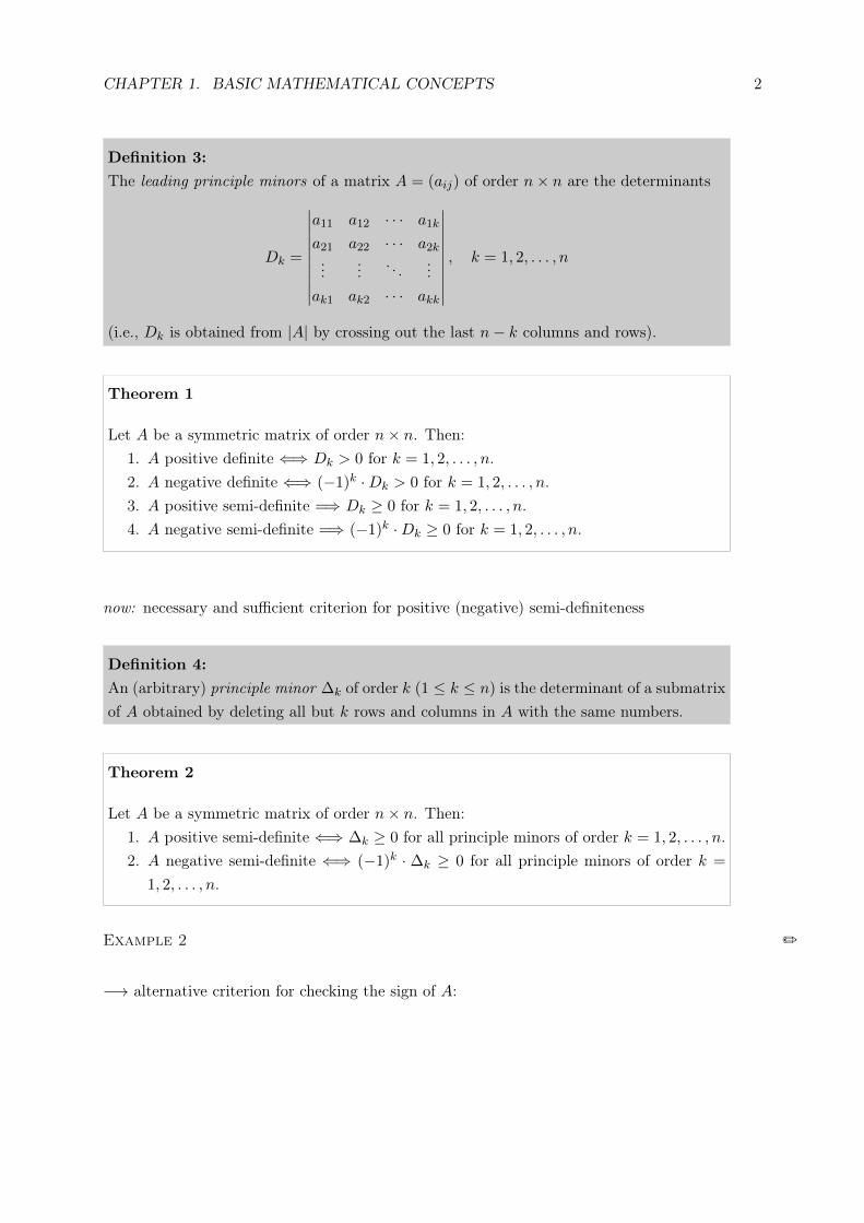
Definition 3:The leading principle minors of a matrix A = (aij) of order n× n are the determinants
Dk =
∣∣∣∣∣∣∣∣∣∣a11 a12 · · · a1k
a21 a22 · · · a2k...
.... . .
...ak1 ak2 · · · akk
∣∣∣∣∣∣∣∣∣∣, k = 1, 2, . . . , n
(i.e., Dk is obtained from |A| by crossing out the last n− k columns and rows).
Theorem 1
Let A be a symmetric matrix of order n× n. Then:1. A positive definite ⇐⇒ Dk > 0 for k = 1, 2, . . . , n.2. A negative definite ⇐⇒ (−1)k ·Dk > 0 for k = 1, 2, . . . , n.3. A positive semi-definite =⇒ Dk ≥ 0 for k = 1, 2, . . . , n.4. A negative semi-definite =⇒ (−1)k ·Dk ≥ 0 for k = 1, 2, . . . , n.
now: necessary and sufficient criterion for positive (negative) semi-definiteness
Definition 4:An (arbitrary) principle minor ∆k of order k (1 ≤ k ≤ n) is the determinant of a submatrixof A obtained by deleting all but k rows and columns in A with the same numbers.
Theorem 2
Let A be a symmetric matrix of order n× n. Then:1. A positive semi-definite ⇐⇒ ∆k ≥ 0 for all principle minors of order k = 1, 2, . . . , n.2. A negative semi-definite ⇐⇒ (−1)k · ∆k ≥ 0 for all principle minors of order k =
1, 2, . . . , n.
Example 2 /
−→ alternative criterion for checking the sign of A:
CHAPTER 1. BASIC MATHEMATICAL CONCEPTS 3
Theorem 3
Let A be a symmetric matrix of order n × n and λ1, λ2, . . . , λn be the real eigenvalues ofA. Then:
1. A positive definite ⇐⇒ λ1 > 0, λ2 > 0, . . . , λn > 0.2. A positive semi-definite ⇐⇒ λ1 ≥ 0, λ2 ≥ 0, . . . , λn ≥ 0.3. A negative definite ⇐⇒ λ1 < 0, λ2 < 0, . . . , λn < 0.4. A negative semi-definite ⇐⇒ λ1 ≤ 0, λ2 ≤ 0, . . . , λn ≤ 0.5. A indefinite ⇐⇒ A has eigenvalues with opposite signs.
Example 3 /
Level curve and tangent line
consider:z = F (x, y)
level curve:F (x, y) = C with C ∈ R
=⇒ slope of the level curve F (x, y) = C at the point (x, y):
y′ = −Fx(x, y)
Fy(x, y)
(See Werner/Sotskov(2006): Mathematics of Economics and Business, Theorem 11.6, implicit-function theorem.)
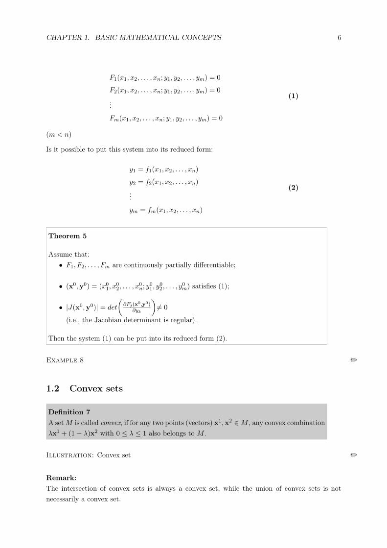
Is it possible to put this system into its reduced form:
y1 = f1(x1, x2, . . . , xn)
y2 = f2(x1, x2, . . . , xn)
...
ym = fm(x1, x2, . . . , xn)
(2)
Theorem 5
Assume that:• F1, F2, . . . , Fm are continuously partially differentiable;
• (x0,y0) = (x01, x02, . . . , x
0n; y01, y
02, . . . , y
0m) satisfies (1);
• |J(x0,y0)| = det
(∂Fj(x
0,y0)∂yk
)6= 0
(i.e., the Jacobian determinant is regular).
Then the system (1) can be put into its reduced form (2).
Example 8 /
1.2 Convex sets
Definition 7A setM is called convex, if for any two points (vectors) x1,x2 ∈M , any convex combinationλx1 + (1− λ)x2 with 0 ≤ λ ≤ 1 also belongs to M .
Illustration: Convex set /
Remark:The intersection of convex sets is always a convex set, while the union of convex sets is notnecessarily a convex set.
CHAPTER 1. BASIC MATHEMATICAL CONCEPTS 7
Illustration: Union and intersection of convex sets /
1.3 Convex and concave functions
Definition 8Let M ⊆ Rn be a convex set.A function f : M −→ R is called convex on M , if
f(λx1 + (1− λ)x2) ≤ λf(x1) + (1− λ)f(x2)
for all x1,x2 ∈M and all λ ∈ [0, 1].f is called concave, if
f(λx1 + (1− λ)x2) ≥ λf(x1) + (1− λ)f(x2)
for all x1,x2 ∈M and all λ ∈ [0, 1].
Illustration: Convex and concave functions /
Definition 9The matrix
Hf (x0) = (fxixj (x0)) =
fx1x1(x0) fx1x2(x0) · · · fx1xn(x0)
fx2x1(x0) fx2x2(x0) · · · fx2xn(x0)...
.... . .
...fxnx1(x0) fxnx2(x0) · · · fxnxn(x0)
is called the Hessian matrix of function f at the point x0 = (x01, x
02, . . . , x
0n) ∈ Df ⊆ Rn.
Remark:If f has continuous second-order partial derivatives, the Hessian matrix is symmetric.
CHAPTER 1. BASIC MATHEMATICAL CONCEPTS 8
Theorem 6
Let f : Df −→ R, Df ⊆ Rn, be twice continuously differentiable and M ⊆ Df be convex.Then:
1. f is convex on M ⇐⇒ the Hessian matrix Hf (x) is positive semi-definite for allx ∈M ;
2. f is concave on M ⇐⇒ the Hessian matrix Hf (x) is negative semi-definite for allx ∈M ;
3. the Hessian matrix Hf (x) is positive definite for all x ∈ M =⇒ f is strictly convexon M ;
4. the Hessian matrix Hf (x) is negative definite for all x ∈M =⇒ f is strictly concaveon M .
Example 9 /
Theorem 7
Let f : M −→ R, g : M −→ R and M ⊆ Rn be a convex set. Then:1. f, g are convex on M and a ≥ 0, b ≥ 0 =⇒ a · f + b · g is convex on M ;2. f, g are concave on M and a ≥ 0, b ≥ 0 =⇒ a · f + b · g is concave on M .
Theorem 8
Let f : M −→ R with M ⊆ Rn being convex and let F : DF −→ R with Rf ⊆ DF . Then:1. f is convex and F is convex and increasing =⇒ (F ◦ f)(x) = F (f(x)) is convex;2. f is convex and F is concave and decreasing =⇒ (F ◦ f)(x) = F (f(x)) is concave;3. f is concave and F is concave and increasing =⇒ (F ◦ f)(x) = F (f(x)) is concave;4. f is concave and F is convex and decreasing =⇒ (F ◦ f)(x) = F (f(x)) is convex.
Example 10 /
1.4 Quasi-convex and quasi-concave functions
Definition 10Let M ⊆ Rn be a convex set and f : M −→ R. For any a ∈ R, the set
Pa = {x ∈M | f(x) ≥ a}
is called an upper level set for f .
Illustration: Upper level set /
CHAPTER 1. BASIC MATHEMATICAL CONCEPTS 9
Theorem 9
Let M ⊆ Rn be a convex set and f : M −→ R. Then:1. If f is concave, then
Pa = {x ∈M | f(x) ≥ a}
is a convex set for any a ∈ R;2. If f is convex, then the lower level set
P a = {x ∈M | f(x) ≤ a}
is a convex set for any a ∈ R.
Definition 11Let M ⊆ Rn be a convex set and f : M −→ R.Function f is called quasi-concave, if the upper level set Pa = {x ∈ M | f(x) ≥ a} isconvex for any number a ∈ R.Function f is called quasi-convex, if −f is quasi-concave.
Remark:f quasi-convex ⇐⇒ the lower level set P a = {x ∈M | f(x) ≤ a} is convex for any a ∈ R
Example 11 /
Remarks:
1. f convex =⇒ f quasi-convexf concave =⇒ f quasi-concave
2. The sum of quasi-convex (quasi-concave) functions is not necessarily quasi-convex (quasi-concave).
Definition 12Let M ⊆ Rn be a convex set and f : M −→ R.Function f is called strictly quasi-concave, if
f(λx1 + (1− λ)x2) > min{f(x1), f(x2)}
for all x1,x2 ∈M with x1 6= x2 and λ ∈ (0, 1).Function f is strictly quasi-convex, if −f is strictly quasi-concave.
CHAPTER 1. BASIC MATHEMATICAL CONCEPTS 10
Remarks:
1. f strictly quasi-concave =⇒ f quasi-concave
2. f : Df −→ R, Df ⊆ R, strictly increasing (decreasing) =⇒ f strictly quasi-concave
3. A strictly quasi-concave function cannot have more than one global maximum point.
Theorem 10
Let f : Df −→ R, Df ⊆ Rn, be twice continuously differentiable on a convex set M ⊆ Rn
and
Br =
∣∣∣∣∣∣∣∣∣∣0 fx1(x) · · · fxr(x)
fx1(x) fx1x1(x) · · · fx1xr(x)...
... · · ·...
fxr(x) fxrx1(x) · · · fxrxr(x)
∣∣∣∣∣∣∣∣∣∣, r = 1, 2, . . . , n
Then:1. A necessary condition for f to be quasi-concave is that (−1)r · Br(x) ≥ 0 for all
x ∈M and all r = 1, 2, . . . , n;2. A sufficient condition for f to be strictly quasi-concave is that (−1)r ·Br(x) > 0 for
all x ∈M and all r = 1, 2, . . . , n.
Example 12 /
Chapter 2
Unconstrained and constrainedoptimization
2.1 Extreme points
Consider:
f(x) −→ min! (or max!)
s.t.x ∈M,
where f : Rn −→ R, ∅ 6= M ⊆ Rn
M - set of feasible solutionsx ∈M - feasible solutionf - objective functionxi, i = 1, 2, . . . , n - decision variables (choice variables)
Definition 1A point x∗ ∈M is called a global minimum point for f in M if
f(x∗) ≤ f(x) for all x ∈M.
The number f∗ := min{f(x) | x ∈M} is called the global minimum.
11
CHAPTER 2. UNCONSTRAINED AND CONSTRAINED OPTIMIZATION 12
similarly:
• global maximum point
• global maximum
(global) extreme point: (global) minimum or maximum point
Theorem 1 (necessary first-order condition)
Let f : M −→ R be differentiable and x∗ = (x∗1, x∗2, . . . , x
∗n) be an interior point of M . A
necessary condition for x∗ to be an extreme point is
Of(x∗) = 0,
i.e., fx1(x∗) = fx2(x∗) = · · · = fxn(x∗) = 0.
Remark:x∗ is a stationary point for f
Theorem 2 (sufficient condition)
Let f : M −→ R with M ⊆ Rn being a convex set. Then:1. If f is convex on M , then:
x∗ is a (global) minimum point for f in M ⇐⇒x∗ is a stationary point for f ;
2. If f is concave on M , then:x∗ is a (global) maximum point for f in M ⇐⇒x∗ is a stationary point for f .
Example 1 /
2.1.2 Local extreme points
Definition 2The set
Uε(x∗) := {x ∈ Rn||x− x∗| < ε}
is called an (open) ε-neighborhood Uε(x∗) with ε > 0.
CHAPTER 2. UNCONSTRAINED AND CONSTRAINED OPTIMIZATION 13
Definition 3A point x∗ ∈ M is called a local minimum point for function f in M if there exists anε > 0 such that
f(x∗) ≤ f(x) for all x ∈M ∩ Uε(x∗).
The number f(x∗) is called a local minimum.
similarly:
• local maximum point
• local maximum
(local) extreme point: (local) minimum or maximum point
Illustration: Global and local minimum points /
Theorem 3 (necessary optimality condition)
Let f be continuously differentiable and x∗ be an interior point ofM being a local minimumor maximum point. Then
Of(x∗) = 0.
Theorem 4 (sufficient optimality condition)
Let f be twice continuously differentiable and x∗ be an interior point of M . Then:1. If Of(x∗) = 0 and H(x∗) is positive definite, then x∗ is a local minimum point.2. If Of(x∗) = 0 and H(x∗) is negative definite, then x∗ is a local maximum point.
Remarks:
1. If H(x∗) is only positive (negative) semi-definite and Of(x∗) = 0, then the above conditionis only necessary.
2. If x∗ is a stationary point and |Hf (x∗)| 6= 0 and neither of the conditions in (1) and (2) ofTheorem 4 are satisfied, then x∗ is a saddle point. The case |Hf (x∗)| = 0 requires furtherexamination.
Example 2 /
CHAPTER 2. UNCONSTRAINED AND CONSTRAINED OPTIMIZATION 14
CHAPTER 2. UNCONSTRAINED AND CONSTRAINED OPTIMIZATION 15
Theorem 6 (sufficient optimality condition)
Let f and gi, i = 1, 2, . . . ,m, be twice continuously differentiable and let (x0;λ0) withx0 ∈ Df be a solution of the system OL(x;λ) = 0.Moreover, let
be the bordered Hessian matrix and consider its leading principle minors Dj(x
0;λ0) of theorder j = 2m+ 1, 2m+ 2, . . . , n+m at point (x0;λ0). Then:
1. If all Dj(x0;λ0), 2m+1 ≤ j ≤ n+m, have the sign (−1)m, then x0 = (x01, x
02, . . . , x
0n)
is a local minimum point of function f subject to the given constraints.2. If all Dj(x
0;λ0), 2m + 1 ≤ j ≤ n + m, alternate in sign, the sign of Dn+m(x0;λ0)
being that of (−1)n, then x0 = (x01, x02, . . . , x
0n) is a local maximum point of function
f subject to the given constraints.3. If neither the condition 1. nor those of 2. are satisfied, then x0 is not a local extreme
point of function f subject to the constraints.Here the case when one or several principle minors have value zero is not consideredas a violation of condition 1. or 2.
special case: n = 2, m = 1 =⇒ 2m+ 1 = n+m = 3
=⇒ consider only D3(x0;λ0)
D3(x0;λ0) < 0 =⇒ sign is (−1)m = (−1)1 = −1
=⇒ x0 is a local minimum point according to 1.
D3(x0;λ0) > 0 =⇒ sign is (−1)n = (−1)2 = 1
=⇒ x0 is a local maximum point according to 2.
Example 3 /
Theorem 7 (sufficient condition for global optimality)
If there exist numbers (λ01, λ02, . . . , λ
0m) = λ0 and an x0 ∈ Df such that OL(x0, λ0) = 0,
then:1. If L(x) = f(x) +
m∑i=1
λ0i · gi(x) is concave in x, then x0 is a maximum point.
2. If L(x) = f(x) +m∑i=1
λ0i · gi(x) is convex in x, then x0 is a minimum point.
CHAPTER 2. UNCONSTRAINED AND CONSTRAINED OPTIMIZATION 16
Example 4 /
2.3 Inequality constraints
Consider:
f(x1, x2, . . . , xn) −→ min!
s.t.
g1(x1, x2, . . . , xn) ≤ 0
g2(x1, x2, . . . , xn) ≤ 0
...
gm(x1, x2, . . . , xn) ≤ 0
(3)
=⇒ L(x;λ) = f(x1, x2, . . . , xn) +
m∑i=1
λi · gi(x1, x2, . . . , xn) = f(x) + λT · g(x),
where
λ =
λ1
λ2...λm
and g(x) =
g1(x)
g2(x)...
gm(x)
Definition 4A point (x∗;λ∗) is called a saddle point of the Lagrangian function L, if
L(x∗;λ) ≤ L(x∗;λ∗) ≤ L(x;λ∗) (2.1)
for all x ∈ Rn, λ ∈ Rm+ .
Theorem 8
If (x∗;λ∗) with λ∗ ≥ 0 is a saddle point of L, then x∗ is an optimal solution of problem(3).
Question: Does any optimal solution correspond to a saddle point?−→ additional assumptions required
Slater condition (S):
There exists a z ∈ Rn such that for all nonlinear constraints gi inequality gi(z) < 0 is satisfied.
CHAPTER 2. UNCONSTRAINED AND CONSTRAINED OPTIMIZATION 17
Remarks:
1. If all constraints g1, . . . , gm are nonlinear, the Slater condition implies that the set M offeasible solutions contains interior points.
2. Condition (S) is one of the constraint qualifications.
Theorem 9 (Theorem by Kuhn and Tucker)
If condition (S) is satisfied, then x∗ is an optimal solution of the convex problem
f(x) −→ min!
s.t.
gi(x) ≤ 0, i = 1, 2, . . . ,m
f, g1, g2, . . . , gm convex functions
(4)
if and only if L has a saddle point (x∗;λ∗) with λ∗ ≥ 0.
Remark:Condition (2.1) is often difficult to check. It is a global condition on the Lagrangian function.If all functions f, g1, . . . , gm are continuously differentiable and convex, then the saddle pointcondition of Theorem 9 can be replaced by the following equivalent local conditions.
Theorem 10
If condition (S) is satisfied and functions f, g1, . . . , gm are continuously differentiableand convex, then x∗ is an optimal solution of problem (4) if and only if the followingKarush-Kuhn-Tucker (KKT)-conditions are satisfied.
Of(x∗) +
m∑i=1
λ∗i · Ogi(x∗) = 0 (2.2)
λ∗i · gi(x∗) = 0 (2.3)
gi(x∗) ≤ 0 (2.4)
λ∗i ≥ 0 (2.5)
i = 1, 2, . . . ,m
Remark:Without convexity of the functions f, g1, . . . , gm the KKT-conditions are only a necessary opti-mality condition, i.e.: If x∗ is a local minimum point, condition (S) is satisfied and functionsf, g1, . . . , gm are continuously differentiable, then the KKT-conditions (2.2)-(2.5) are satisfied.
CHAPTER 2. UNCONSTRAINED AND CONSTRAINED OPTIMIZATION 18
Summary:
(x∗;λ∗) satisfies theKKT-conditions, problem is
convex
=⇒ x∗ is a global minimum point
x∗ local minimum point,condition (S) is satisfied
=⇒ KKT-conditions are satisfied
Example 5 /
2.4 Non-negativity constraints
Consider a problem with additional non-negativity constraints:
f(x) −→ min!
s.t.
gi(x) ≤ 0, i = 1, 2, . . . ,m
x ≥ 0
(5)
Example 6 /
−→ To find KKT-conditions for problem (5) introduce a Lagrangian multiplier µj for any non-negativity constraint xj ≥ 0 which corresponds to −xj ≤ 0.
KKT-conditions:
Of(x∗) +m∑i=1
λ∗iOgi(x∗)− µ∗ = 0 (2.6)
λ∗i · gi(x∗) = 0, i = 1, 2, . . . ,m (2.7)
µ∗j · x∗j = 0, j = 1, 2, . . . , n (2.8)
gi(x∗) ≤ 0 (2.9)
x∗ ≥ 0, λ∗ ≥ 0, µ∗ ≥ 0 (2.10)
CHAPTER 2. UNCONSTRAINED AND CONSTRAINED OPTIMIZATION 19
Using (2.6) to (2.10), we can rewrite the KKT-conditions as follows:
Of(x∗) +
m∑i=1
λ∗iOgi(x∗) ≥ 0
λ∗i · gi(x∗) = 0, i = 1, 2, . . . ,m
x∗j ·(∂f
∂xj(x∗) +
m∑i=1
λ∗i ·∂gi∂xj
(x∗)
)= 0, j = 1, 2, . . . , n
gi(x∗) ≤ 0
x∗ ≥ 0, λ∗ ≥ 0
i.e., the new Lagrangian multipliers µj have been eliminated.
Example 7 /
Some comments on quasi-convex programming
Theorem 11
Consider a problem (5), where function f is continuously differentiable and quasi-convex.Assume that there exist numbers λ∗1, λ∗2, . . . , λ∗m and a vector x∗ such that
1. the KKT-conditions are satisfied;2. Of(x∗) 6= 0;3. λ∗i · gi(x) is quasi-convex for i = 1, 2, . . . ,m.
Then x∗ is optimal for problem (5).
Remark:Theorem 11 holds analogously for problem (3).
Chapter 3
Sensitivity analysis
3.1 Preliminaries
Question: How does a change in the parameters affect the solution of an optimization problem?
−→ sensitivity analysis (in optimization)
−→ comparative statics (or dynamics) (in economics)
Example 1 /
3.2 Value functions and envelope results
3.2.1 Equality constraints
Consider:
f(x; r) −→ min!
s.t.
gi(x; r) = 0, i = 1, 2, . . . ,m
where r = (r1, r2, . . . , rk)T - vector of parameters
(6)
Remark:In (6), we optimize w.r.t. x with r held constant.
Notations:
x1(r), x2(r), . . . , xn(r) - optimal solution in dependence on r
f∗(r) = f(x1(r), x2(r), . . . , xn(r)) - (minimum) value function
20
CHAPTER 3. SENSITIVITY ANALYSIS 21
λi(r) (i = 1, 2, . . . ,m) - Lagrangian multipliers in the necessary optimality condition
Lagrangian function:
L(x;λ; r) = f(x; r) +m∑i=1
λi · gi(x; r)
= f(x(r); r) +m∑i=1
λi(r) · gi(x(r); r) = L∗(r)
Theorem 1 (Envelope Theorem for equality constraints)
For j = 1, 2, . . . , k, we have:
∂f∗(r)
∂rj=
(∂L(x;λ; r)
∂rj
)∣∣∣(x(r)λ(r))
=∂L∗(r)
∂rj
Remark:Notice that ∂L∗
∂rjmeasures the total effect of a change in rj on the Lagrangian function, while ∂L
∂rj
measures the partial effect of a change in rj on the Lagrangian function with x and λ being heldconstant.
Example 2 /
3.2.2 Properties of the value function for inequality constraints
Consider:f(x, r) −→ min!
s.t.gi(x, r) ≤ 0, i = 1, 2, . . . ,m
minimum value function:b −→ f∗(b)
f∗(b) = min{f(x) | gi(x)− bi ≤ 0, i = 1, 2, . . . ,m}
x(b) - optimal solution
λi(b) - corresponding Lagrangian multipliers
=⇒ ∂f∗(b)
∂bi= −λi(b), i = 1, 2, . . . ,m
Remark:Function f∗ is not necessarily continuously differentiable.
CHAPTER 3. SENSITIVITY ANALYSIS 22
Theorem 2
If function f(x) is concave and functions g1(x), g2(x), . . . , gm(x) are convex, then functionf∗(b) is concave.
Example 3: /
A firm has L units of labour available and produces 3 goods whose values per unit of output area, b and c, respectively. Producing x, y and z units of the goods requires αx2, βy2 and γz2 unitsof labour, respectively. We maximize the value of output and determine the value function.
f∗(r) = min {f(x, r) = f(x1(r), x2(r), . . . , xn(r)) | x ∈M(r)}
Lagrangian function:
L(x;λ; r) = f(x; r) +
m∑i=1
λi · gi(x; r)
= f(x(r); r) +
m∑i=1
λi(r) · gi(x(r); r) = L∗(r)
Theorem 3 (Envelope Theorem for mixed constraints)
For j = 1, 2, . . . , k, we have:
∂f∗(r)
∂rj=
(∂L(x;λ; r)
∂rj
)∣∣∣(x(r)λ(r))
=∂L∗(r)
∂rj
Example 4 /
CHAPTER 3. SENSITIVITY ANALYSIS 23
3.3 Some further microeconomic applications
3.3.1 Cost minimization problem
Consider:C(w,x) = wT · x(w, y) −→ min!
s.t.y − f(x) ≤ 0
x ≥ 0, y ≥ 0
• Assume that w > 0 and that the partial derivatives of C are > 0.
• Let x(w, y) be the optimal input vector and λ(w, y) be the corresponding Lagrangianmultiplier.
L(x;λ;w, y) = wT · x + λ · (y − f(x))
=⇒ ∂C
∂y=∂L
∂y= λ = λ(w, y) (3.1)
i.e., λ signifies marginal costs
Shepard(-McKenzie) Lemma:
∂C
∂wi= xi = xi(w, y), i = 1, 2, . . . , n (3.2)
Remark:Assume that C is twice continuously differentiable. Then the Hessian HC is symmetric.
Differentiating (3.1) w.r.t. wi and (3.2) w.r.t. y, we obtain
Samuelson’s reciprocity relation:
=⇒ ∂xj∂wi
=∂xi∂wj
and∂xi∂y
=∂λ
∂wi, for all i and j
Interpretation of the first result:
A change in the j-th factor input w.r.t. a change in the i-th factor price (output being constant)must be equal to the change in the i-th factor input w.r.t. a change in the j-th factor price.
CHAPTER 3. SENSITIVITY ANALYSIS 24
3.3.2 Profit maximization problem of a competitive firm
Consider:π(x,y) = pT · y −wT · x −→ max! (−π −→ min!)
s.t.g(x,y) = y − f(x) ≤ 0
x ≥ 0, y ≥ 0,
where:
p > 0 - output price vectorw > 0 - input price vectory ∈ Rm+ - produced vector of outputx ∈ Rn+ - used input vectorf(x) - production function
Let:
x(p,w),y(p,w) be the optimal solutions of the problem andπ(p,w) = pT · y(p,w)−wT · x(p,w) be the (maximum) profit function.
L(x,y;λ;p,w) = −pTy + wTx + λ · (y − f(x))
The Envelope theorem implies
Hotelling’s lemma:
1.∂(−π)
∂pi=∂L
∂pi= −yi i.e.:
∂π
∂pi= yi > 0, i = 1, 2, . . . ,m (3.3)
2.∂(−π)
∂wi=
∂L
∂wi= xi i.e.:
∂π
∂wi= −xi < 0, i = 1, 2, . . . ,m (3.4)
Interpretation:
1. An increase in the price of any output increases the maximum profit.
2. An increase in the price of any input lowers the maximum profit.
Remark:Let π(p,w) be twice continuously differentiable. Using (3.3) and (3.4), we obtain
Hotelling’s symmetry relation:
∂yj∂pi
=∂yi∂pj
,∂xj∂wi
=∂xi∂wj
,∂xj∂pi
= − ∂yi∂wj
, for all i and j.
Chapter 4
Applications to consumer choice andgeneral equilibrium theory
4.1 Some aspects of consumer choice theory
Consumer choice problem
Let:
x ∈ Rn+ - commodity bundle of consumption
U(x) - utility function
p ∈ Rn+ - price vector
I - income
Then:U(x) −→ max! (−U(x) −→ min!)
s.t.pT · x ≤ I (g(x) = pT · x− I ≤ 0)
x ≥ 0
assumption: U quasi-concave (=⇒ −U quasi-convex)
L(x;λ) = −U(x) + λ(pT · x− I)
KKT-conditions:−Uxi(x) + λpi ≥ 0 (4.1)
λ(pT · x− I) = 0 (4.2)
25
CHAPTER 4. CONSUMER CHOICE AND GENERAL EQUILIBRIUM THEORY 26
xi(−Uxi(x) + λpi) = 0
pT · x− I ≤ 0
x ≥ 0, λ ≥ 0
Suppose that OU(x∗) 6= 0 and that x∗ is feasible.Thm. 11, Ch.2
=⇒ x∗ solves the problem and satisfies the KKT-conditions.
If additionally Uxi(x∗) ≥ 0 is assumed for i = 1, 2, . . . , n
OU(x∗) 6=0=⇒ There exists a j such that Uxj (x∗) > 0
(4.1)=⇒ λ > 0
(4.2)=⇒ pT · x = I, i.e., all income is spent.
Consider now the following version of the problem:
U(x) −→ max!
s.t.pT · x = I
x ≥ 0
Let:
rT = (p, I) - vector of parameters
x∗ = x(p, I) - optimal solution
λ(p, I) - corresponding Lagrangian multiplier
−→ maximum value U depends on p and I:
U∗ = U(x(p, I)) − indirect utility function
We determine∂U∗
∂Iand
∂U∗
∂pi
L(x;λ;p, I) = −U(x;p, I) + λ(I − pTx)
∂L
∂I∣∣∣(x(p,I)λ(p,I))
= λ = λ(p, I).
CHAPTER 4. CONSUMER CHOICE AND GENERAL EQUILIBRIUM THEORY 27
Thm. 1,Ch. 3=⇒ ∂(−U∗)
∂I= λ =⇒ ∂U∗
∂I= −λ (4.3)
Thm. 1,Ch. 3=⇒ ∂(−U∗)
∂pi=∂L
∂pi∣∣∣(x(p,I)λ(p,I))
= −λx∗i , i = 1, 2, . . . , n (4.4)
(4.3),(4.4)=⇒ ∂(−U∗)
∂pi+ x∗i
∂(−U∗)∂I
= 0︸ ︷︷ ︸ROY’s identity
Pareto-efficient allocation of commodities
Let:
U i(x) = U i(x1, x2, . . . , xl) - utility function of consumer i = 1, 2, . . . , k in dependence on theamounts xj of commodity j, j = 1, 2, . . . , l
Definition 1An allocation x = (x1, x2, . . . , xl) is said to be pareto-efficient (or pareto-optimal), ifthere does not exist an allocation x∗ = (x∗1, x
∗2, . . . , x
∗l ) such that U i(x∗) ≥ U i(x) for
i = 1, 2, . . . , k and U i(x∗) > U i(x) for at least one i ∈ {1, 2, . . . , k}.If such an allocation x∗ would exist, x∗ is said to be pareto-superior to x.
Preference relation %: x∗ % x (x∗ is preferred to x or they are indifferent)
The Edgeworth box
• efficient allocation of commodities among customers (or of resources in production)
• two customers (k = 2) and two commodities (l = 2)
• graph indifference (level) curves U i =const. into a coordinate system
Illustration: Edgeworth box /
Characterization of pareto-efficient allocations
They correspond to those points, where the slopes of the indifference curves of both customerscoincide.
Definition 2The contract curve is defined as the set of all points which represent pareto-efficient allo-cations of the commodities.
CHAPTER 4. CONSUMER CHOICE AND GENERAL EQUILIBRIUM THEORY 28
Remark:The contract curve describes all equilibrium allocations.
Illustration: Contract curve /
similarly: market price system
Here prices adjust, so that supply equals demand in all markets.
4.2 Fundamental theorems of welfare economics
4.2.1 Notations and preliminaries
Consider an exchange economy with n (goods) markets.
p = (p1, p2, . . . , pn), pi > 0, i = 1, 2, . . . , n - price vectork consumers (households) i ∈ I = {1, 2, . . . , k}l producers j ∈ J = {1, 2, . . . , l}
Let:
• xi = (xi1, xi2, . . . , x
in) ∈ Rn+ - consumption bundle and
U i = U i(xi) ∈ R - utility function of consumer i ∈ I.
• yj = (yj1, yj2, . . . , y
jn) ∈ Rn+ - technology of firm j ∈ J .
• e = (e1, e2, . . . , en) ∈ Rn+ - (initial) endowment andei = (ei1, e
i2, . . . , e
in) ∈ Rn+ - endowment of consumer i ∈ I.
Pure exchange economy:E =
[(xi, U i)i∈I , (yj)j∈J , e
]
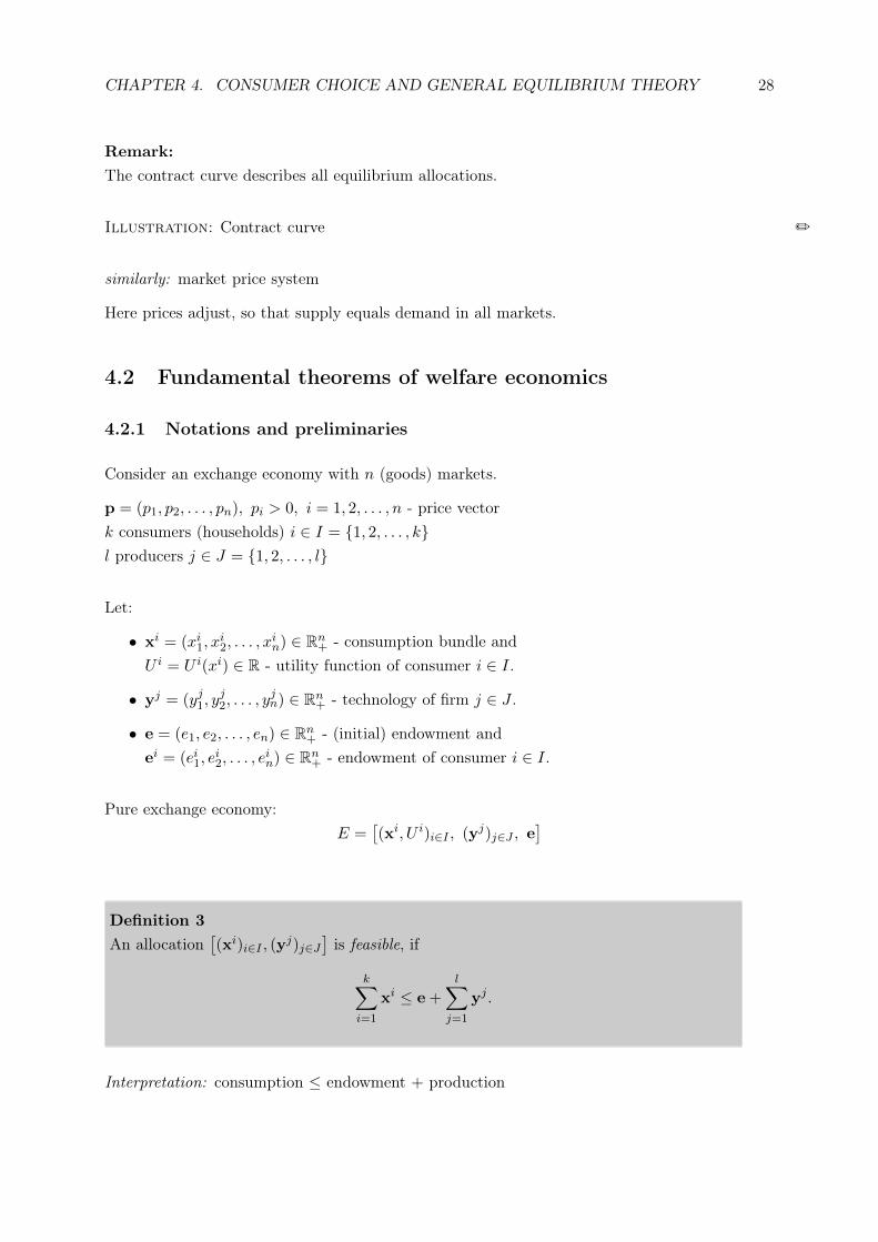
Definition 3An allocation
[(xi)i∈I , (y
j)j∈J]is feasible, if
k∑i=1
xi ≤ e +
l∑j=1
yj .
Interpretation: consumption ≤ endowment + production
CHAPTER 4. CONSUMER CHOICE AND GENERAL EQUILIBRIUM THEORY 29
Competitive economy with private ownership
Each consumer (household) i ∈ I is characterized by
• an endowment ei = (ei1, ei2, . . . , e
in) ∈ Rn+ and
• the ownership share αij of firm j (j ∈ J): αi = (αi1, . . . , α1l ).
Competitive equilibrium for E∗
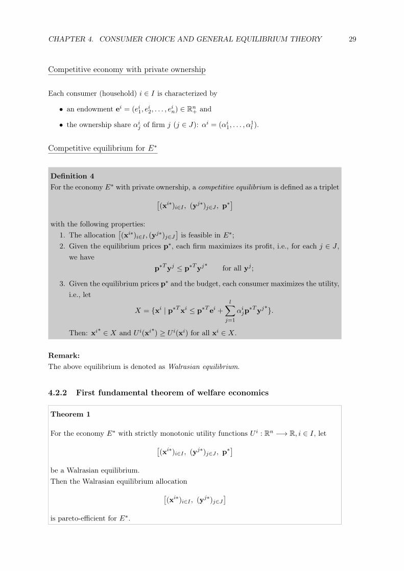
Definition 4For the economy E∗ with private ownership, a competitive equilibrium is defined as a triplet[
(xi∗)i∈I , (yj∗)j∈J , p∗]
with the following properties:1. The allocation
[(xi∗)i∈I , (y
j∗)j∈J]is feasible in E∗;
2. Given the equilibrium prices p∗, each firm maximizes its profit, i.e., for each j ∈ J ,we have
p∗Tyj ≤ p∗Tyj∗ for all yj ;
3. Given the equilibrium prices p∗ and the budget, each consumer maximizes the utility,i.e., let
X = {xi | p∗Txi ≤ p∗Tei +l∑
j=1
αijp∗Tyj
∗}.
Then: xi∗ ∈ X and U i(xi∗) ≥ U i(xi) for all xi ∈ X.
Remark:The above equilibrium is denoted as Walrasian equilibrium.
4.2.2 First fundamental theorem of welfare economics
Theorem 1
For the economy E∗ with strictly monotonic utility functions U i : Rn −→ R, i ∈ I, let[(xi∗)i∈I , (yj∗)j∈J , p
∗]be a Walrasian equilibrium.Then the Walrasian equilibrium allocation[
(xi∗)i∈I , (yj∗)j∈J]
is pareto-efficient for E∗.
CHAPTER 4. CONSUMER CHOICE AND GENERAL EQUILIBRIUM THEORY 30
Interpretation: Theorem 1 states that any Walrasian equilibrium leads to a pareto-efficientallocation of resources.
Remark:Theorem 1 does not require convexity of tastes (preferences) and technologies.
4.2.3 Second fundamental theorem of welfare economics
−→ Consider a more abstract economy with transfers (e.g. positive/negative taxes).
Let:
w = (w1, w2, . . . , wk) ∈ Rk - wealth vector
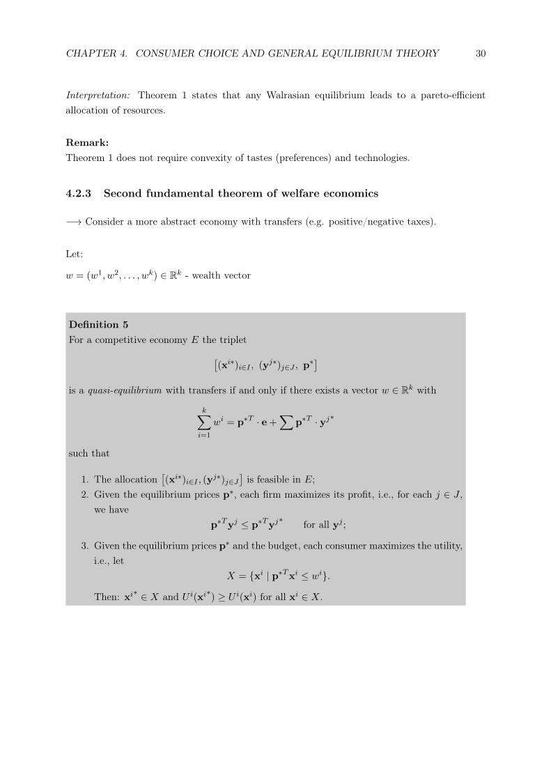
Definition 5For a competitive economy E the triplet[
(xi∗)i∈I , (yj∗)j∈J , p∗]
is a quasi-equilibrium with transfers if and only if there exists a vector w ∈ Rk with
k∑i=1
wi = p∗T · e +∑
p∗T · yj∗
such that
1. The allocation[(xi∗)i∈I , (y
j∗)j∈J]is feasible in E;
2. Given the equilibrium prices p∗, each firm maximizes its profit, i.e., for each j ∈ J ,we have
p∗Tyj ≤ p∗Tyj∗ for all yj ;
3. Given the equilibrium prices p∗ and the budget, each consumer maximizes the utility,i.e., let
X = {xi | p∗Txi ≤ wi}.
Then: xi∗ ∈ X and U i(xi∗) ≥ U i(xi) for all xi ∈ X.
CHAPTER 4. CONSUMER CHOICE AND GENERAL EQUILIBRIUM THEORY 31
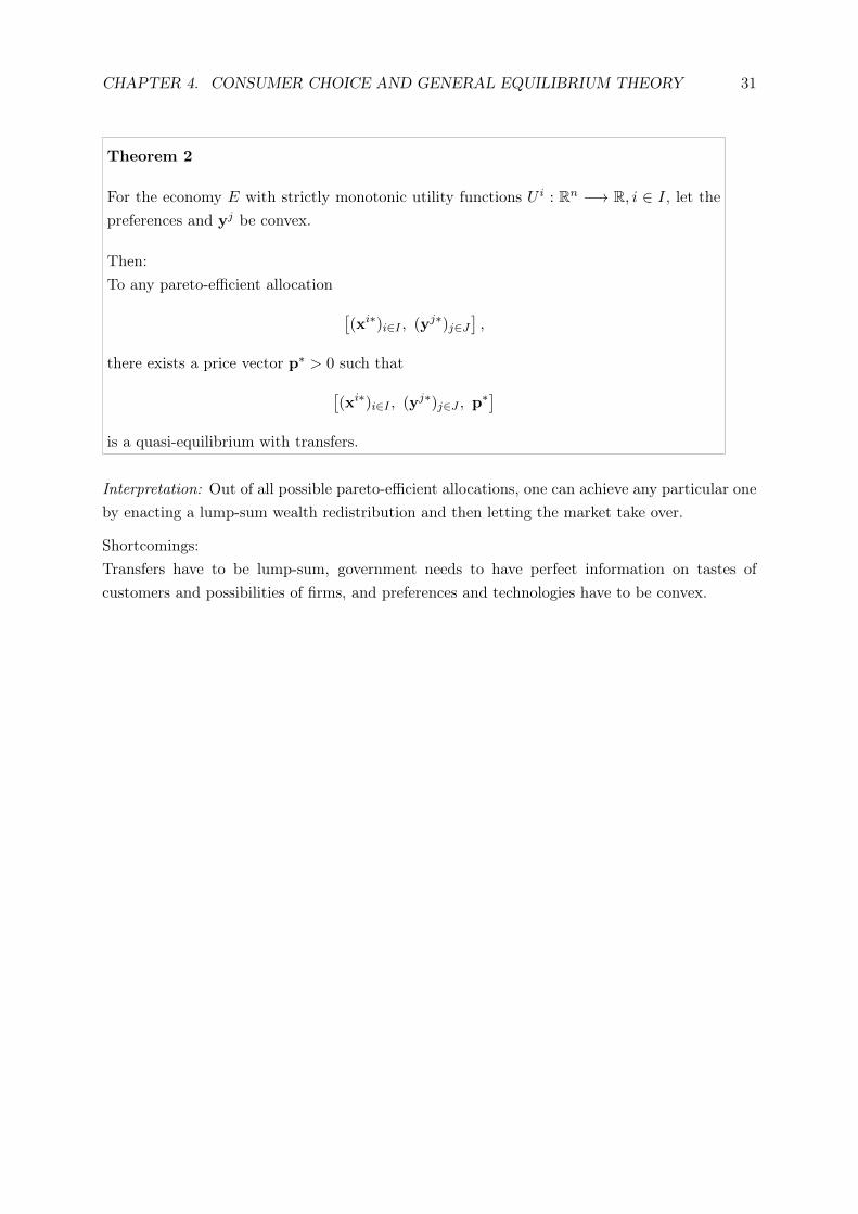
Theorem 2
For the economy E with strictly monotonic utility functions U i : Rn −→ R, i ∈ I, let thepreferences and yj be convex.
Then:To any pareto-efficient allocation [
(xi∗)i∈I , (yj∗)j∈J],
there exists a price vector p∗ > 0 such that[(xi∗)i∈I , (yj∗)j∈J , p
∗]is a quasi-equilibrium with transfers.
Interpretation: Out of all possible pareto-efficient allocations, one can achieve any particular oneby enacting a lump-sum wealth redistribution and then letting the market take over.
Shortcomings:Transfers have to be lump-sum, government needs to have perfect information on tastes ofcustomers and possibilities of firms, and preferences and technologies have to be convex.
Chapter 5
Differential equations
5.1 Preliminaries
Definition 1A relationship
F (x, y, y′, y′′, . . . , y(n)) = 0
between the independent variable x, a function y(x) and its derivatives is called an ordinarydifferential equation. The order of the differential equation is determined by the highestorder of the derivatives appearing in the differential equation.
Definition 2A function y(x) for which the relationship F (x, y, y′, y′′, . . . , y(n)) = 0 holds for all x ∈ Dy
is called a solution of the differential equation.The set
S = {y(x) | F (x, y, y′, y′′, . . . , y(n)) = 0 for all x ∈ Dy}
is called the set of solutions or the general solution of the differential equation.
in economics often:
time t is the independent variable, solution x(t) with
x =dx
dt, x =
d2x
dt2, etc.
32
CHAPTER 5. DIFFERENTIAL EQUATIONS 33
5.2 Differential equations of the first order
implicit form:F (t, x, x) = 0
explicit form:x = f(t, x)
Graphical solution:
given: x = f(t, x)
At any point (t0, x0) the value x = f(t0, x0) is given, which corresponds to the slope of thetangent at point (t0, x0).
−→ graph the direction field (or slope field)
Example 2 /
5.2.1 Separable equations
x = f(t, x) = g(t) · h(x)
=⇒∫
dx
h(x)=
∫g(t) · dt
=⇒ H(x) = G(t) + C
−→ solve for x (if possible)
x(t0) = x0 given:
−→ C is assigned a particular value
=⇒ xp - particular solution
Example 3 /
Example 4 /
5.2.2 First-order linear differential equations
x+ a(t) · x = q(t) q(t) - forcing term
CHAPTER 5. DIFFERENTIAL EQUATIONS 34
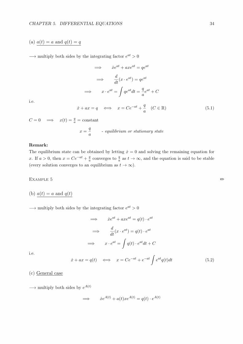
(a) a(t) = a and q(t) = q
−→ multiply both sides by the integrating factor eat > 0
=⇒ xeat + axeat = qeat
=⇒ d
dt(x · eat) = qeat
=⇒ x · eat =
∫qeatdt =
q
aeat + C
i.e.x+ ax = q ⇐⇒ x = Ce−at +
q
a(C ∈ R) (5.1)
C = 0 =⇒ x(t) = qa = constant
x =q
a- equilibrium or stationary state
Remark:The equilibrium state can be obtained by letting x = 0 and solving the remaining equation forx. If a > 0, then x = Ce−at + q
a converges to qa as t→∞, and the equation is said to be stable
(every solution converges to an equilibrium as t→∞).
Example 5 /
(b) a(t) = a and q(t)
−→ multiply both sides by the integrating factor eat > 0
=⇒ xeat + axeat = q(t) · eat
=⇒ d
dt(x · eat) = q(t) · eat
=⇒ x · eat =
∫q(t) · eatdt+ C
i.e.x+ ax = q(t) ⇐⇒ x = Ce−at + e−at
∫eatq(t)dt (5.2)
(c) General case
−→ multiply both sides by eA(t)
=⇒ xeA(t) + a(t)xeA(t) = q(t) · eA(t)
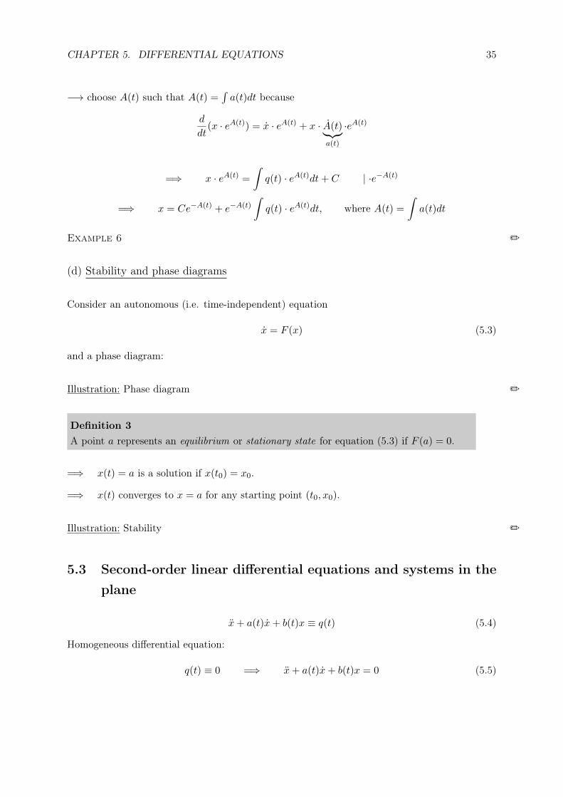
CHAPTER 5. DIFFERENTIAL EQUATIONS 35
−→ choose A(t) such that A(t) =∫a(t)dt because
d
dt(x · eA(t)) = x · eA(t) + x · A(t)︸︷︷︸
a(t)
·eA(t)
=⇒ x · eA(t) =
∫q(t) · eA(t)dt+ C | ·e−A(t)
=⇒ x = Ce−A(t) + e−A(t)∫q(t) · eA(t)dt, where A(t) =
∫a(t)dt
Example 6 /
(d) Stability and phase diagrams
Consider an autonomous (i.e. time-independent) equation
x = F (x) (5.3)
and a phase diagram:
Illustration: Phase diagram /
Definition 3A point a represents an equilibrium or stationary state for equation (5.3) if F (a) = 0.
=⇒ x(t) = a is a solution if x(t0) = x0.
=⇒ x(t) converges to x = a for any starting point (t0, x0).
Illustration: Stability /
5.3 Second-order linear differential equations and systems in theplane
x+ a(t)x+ b(t)x ≡ q(t) (5.4)
Homogeneous differential equation:
q(t) ≡ 0 =⇒ x+ a(t)x+ b(t)x = 0 (5.5)
CHAPTER 5. DIFFERENTIAL EQUATIONS 36
Theorem 1
The homogeneous differential equation (5.5) has the general solution
xH(t) = C1x1(t) + C2x2(t), C1, C2 ∈ R
where x1(t), x2(t) are two solutions that are not proportional (i.e., linearly independent).The non-homogeneous equation (5.4) has the general solution
where xN (t) is any particular solution of the non-homogeneous equation.
(a) Constant coefficients a(t) = a and b(t) = b
x+ ax+ bx = q(t)
Homogeneous equation:x+ ax+ bx = 0
−→ use the setting x(t) = eλt (λ ∈ R)
=⇒ x(t) = λeλt, x(t) = λ2eλt
=⇒ Characteristic equation:λ2 + aλ+ b = 0 (5.6)
3 cases:
1. (5.6) has two distinct real roots λ1, λ2
=⇒ xH(t) = C1eλ1t + C2e
λ2t
2. (5.6) has a real double root λ1 = λ2
=⇒ xH(t) = C1eλ1t + C2te
λ1t
3. (5.6) has two complex roots λ1 = α+ β · i and λ2 = α− β · i
xH(t) = eαt(C1 cosβt+ C2 sinβt)
Non-homogeneous equation:x+ ax+ bx = q(t)
CHAPTER 5. DIFFERENTIAL EQUATIONS 37
Discussion of special forcing terms:
Forcing term q(t) Setting xN (t)
1. q(t) = p · est(a) xN (t) = A · est - if s is not a root of the characteristic
equation(b) xN (t) = A · tkest - if s is a root of multiplicity k
(k ≤ 2) of the characteristic equation
2. q(t) =
pntn+pn−1t
n−1+ · · ·+p1t+p0(a) xN (t) = Ant
n +An−1tn−1 + · · ·+A1t+A0 - if b 6= 0
in the homogeneous equation(b) xN (t) = tk · (Antn +An−1t
n−1 + · · ·+A1t+A0) -with k = 1 if a 6= 0, b = 0 and k = 2 if a = b = 0
3. q(t) = p cos st+ r sin st(a) xN (t) = A cos st+B sin st - if si is not a root of the
characteristic equation(b) xN (t) = tk · (A cos st+B sin st) - if si is a root of
multiplicity k of the characteristic equation
−→ Use the above setting and insert it and the derivatives into the non-homogeneous equation.Determine the coefficients A,B and Ai, respectively.
Example 7 /
(b) Stability
Consider equation (5.4)
Definition 4Equation (5.4) is called globally asymptotically stable if every solution xH(t) = C1x1(t) +
C2x2(t) of the associated homogeneous equation tends to 0 as t → ∞ for all values of C1
and C2.
Remark:xH(t)→ 0 as t→∞ ⇐⇒ x1(t)→ 0 and x2(t)→ 0 as t→∞
Example 8 /
CHAPTER 5. DIFFERENTIAL EQUATIONS 38
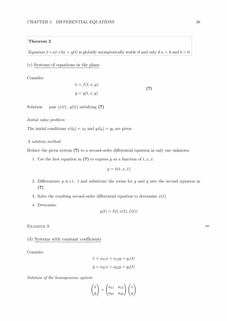
Theorem 2
Equation x+ax+bx = q(t) is globally asymptotically stable if and only if a > 0 and b > 0.
(c) Systems of equations in the plane
Consider:
x = f(t, x, y)
y = g(t, x, y)(7)
Solution: pair (x(t), y(t)) satisfying (7)
Initial value problem:
The initial conditions x(t0) = x0 and y(t0) = y0 are given.
A solution method:
Reduce the given system (7) to a second-order differential equation in only one unknown.
1. Use the first equation in (7) to express y as a function of t, x, x.
y = h(t, x, x)
2. Differentiate y w.r.t. t and substitute the terms for y and y into the second equation in(7).
3. Solve the resulting second-order differential equation to determine x(t).
4. Determiney(t) = h(t, x(t), x(t))
Example 9 /
(d) Systems with constant coefficients
Consider:x = a11x+ a12y + q1(t)
y = a21x+ a22y + q2(t)
Solution of the homogeneous system:(x
y
)=
(a11 a12
a21 a22
)(x
y
)
CHAPTER 5. DIFFERENTIAL EQUATIONS 39
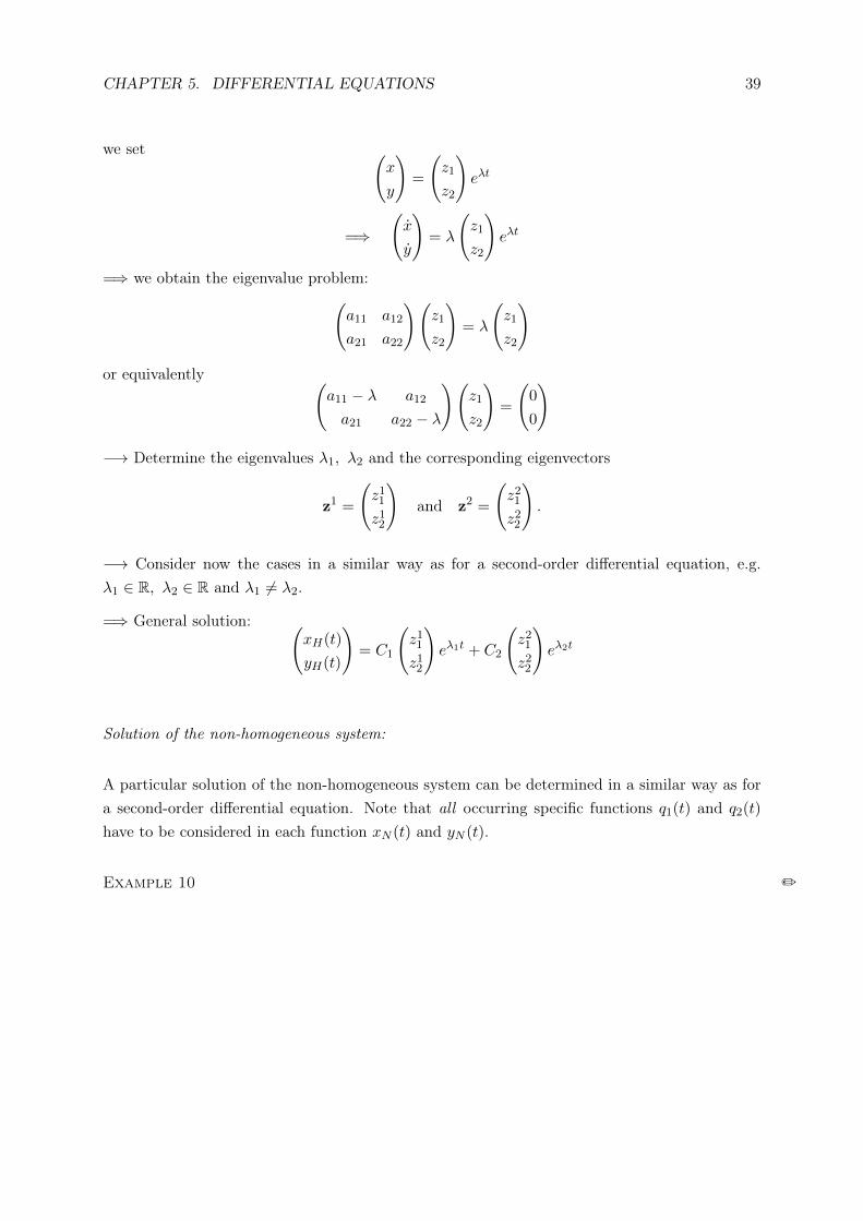
we set (x
y
)=
(z1
z2
)eλt
=⇒
(x
y
)= λ
(z1
z2
)eλt
=⇒ we obtain the eigenvalue problem:(a11 a12
a21 a22
)(z1
z2
)= λ
(z1
z2
)
or equivalently (a11 − λ a12
a21 a22 − λ
)(z1
z2
)=
(0
0
)
−→ Determine the eigenvalues λ1, λ2 and the corresponding eigenvectors
z1 =
(z11z12
)and z2 =
(z21z22
).
−→ Consider now the cases in a similar way as for a second-order differential equation, e.g.λ1 ∈ R, λ2 ∈ R and λ1 6= λ2.
=⇒ General solution: (xH(t)
yH(t)
)= C1
(z11z12
)eλ1t + C2
(z21z22
)eλ2t
Solution of the non-homogeneous system:
A particular solution of the non-homogeneous system can be determined in a similar way as fora second-order differential equation. Note that all occurring specific functions q1(t) and q2(t)
have to be considered in each function xN (t) and yN (t).
Example 10 /
CHAPTER 5. DIFFERENTIAL EQUATIONS 40
(e) Equilibrium points for linear systems with constant coefficients and forcing term
Consider:x = a11x+ a12y + q1
y = a21x+ a22y + q2
For finding an equilibrium point (state), we set x = y = 0 and obtain
a11x+ a12y = −q1
a21x+ a22y = −q2
Cramer’s rule=⇒ equilibrium point:
x∗ =
∣∣∣∣∣−q1 a12
−q2 a22
∣∣∣∣∣∣∣∣∣∣a11 a12
a21 a22
∣∣∣∣∣=a12q2 − a22q1
|A|
y∗ =
∣∣∣∣∣a11 −q1a21 −q2
∣∣∣∣∣∣∣∣∣∣a11 a12
a21 a22
∣∣∣∣∣=a21q1 − a11q2
|A|
Example 11 /
Theorem 3
Suppose that |A| 6= 0. Then the equilibrium point (x∗, y∗) for the linear system
x = a11x+ a12y + q1
y = a21x+ a22y + q2
is globally asymptotically stable if and only if
tr(A) = a11 + a22 < 0 and |A| =
∣∣∣∣∣a11 a12
a21 a22
∣∣∣∣∣ > 0,
where tr(A) is the trace of A (or equivalently, if and only if both eigenvalues of A havenegative real parts).
Example 12 /
CHAPTER 5. DIFFERENTIAL EQUATIONS 41
(f) Phase plane analysis
Consider an autonomous system:x = f(x, y)
y = g(x, y)
−→ Rates of change of x(t) and y(t) are given by f(x(t), y(t)) and g(x(t), y(t)), e.g.
if f(x(t), y(t)) > 0 and g(x(t), y(t)) < 0 at a point P = (x(t), y(t)), then (as t increases) thesystem will move from point P down and to the right.
=⇒ (x(t), y(t)) gives direction of motion, length of (x(t), y(t)) gives speed of motion
Illustration: Motion of a system /
Graph a sample of these vectors. =⇒ phase diagram
Equilibrium point: point (a, b) with f(a, b) = g(a, b) = 0
−→ equilibrium points are the points of the intersection of the nullclinesf(x, y) = 0 and g(x, y) = 0
−→ Graph the nullclines:
• At point P with f(x, y) = 0, x = 0 and the velocity vector is vertical, it points up if y > 0
and down if y < 0.
• At point Q with g(x, y) = 0, y = 0 and the velocity vector is horizontal, it points to theright if x > 0 and to the left if x < 0.
−→ Continue and graph further arrows.
Example 13 /
Chapter 6
Optimal control theory
6.1 Calculus of variations
Consider:t1∫t0
F (t, x, x)dt −→ max!
s.t.x(t0) = x0, x(t1) = x1
(8)
Illustration /
necessary optimality condition:
Function x(t) can only solve problem (8) if x(t) satisfies the following differential equation.
−→ Euler equation:∂F
∂x− d
dt
(∂F
∂x
)= 0 (6.1)
we haved
dt
(∂F (t, x, x)
∂x
)=
∂2F
∂t∂x+
∂2F
∂x∂x· x+
∂2F
∂x∂x· x
=⇒ (6.1) can be rewritten as
∂2F
∂x∂x· x+
∂2F
∂x∂x· x+
∂2F
∂t∂x− ∂F
∂x= 0
42
CHAPTER 6. OPTIMAL CONTROL THEORY 43
Theorem 1
If F (t, x, x) is concave in (x, x), a feasible x∗(t) that satisfies the Euler equation solves themaximization problem (8).
Example 1 /
More general terminal conditions
Consider:t1∫t0
F (t, x, x)dt −→ max!
s.t.x(t0) = x0
(a) x(t1) free or (b) x(t1) ≥ x1
(9)
Illustration /
=⇒ transversality condition needed to determine the second constant
Theorem 2 (Transversality conditions)
If x∗(t) solves problem (9) with either (a) or (b) as the terminal condition, then x∗(t) mustsatisfy the Euler equation.With the terminal condition (a), the transversality condition is(
∂F ∗
∂x
)t=t1
= 0. (6.2)
With the terminal condition (b), the transversality condition is(∂F ∗
∂x
)t=t1
≤ 0
[(∂F ∗
∂x
)t=t1
= 0, if x∗(t1) > x1
](6.3)
If F (t, x, x) is concave in (x, x), then a feasible x∗(t) that satisfies both the Euler equation andthe appropriate transversality condition will solve problem (9).
Example 2 /
CHAPTER 6. OPTIMAL CONTROL THEORY 44
6.2 Control theory
6.2.1 Basic problem
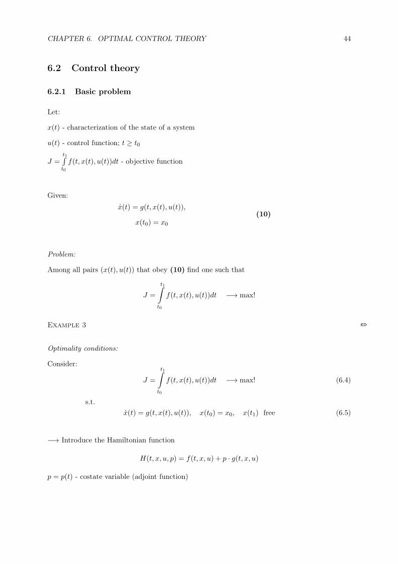
Let:
x(t) - characterization of the state of a system
u(t) - control function; t ≥ t0
J =t1∫t0
f(t, x(t), u(t))dt - objective function
Given:
x(t) = g(t, x(t), u(t)),
x(t0) = x0
(10)
Problem:
Among all pairs (x(t), u(t)) that obey (10) find one such that
H(t, x, u, p(t)) is concave in (x, u) for each t ∈ [t0, t1] (6.8)
is added to the conditions in Theorem 3, we obtain a sufficient optimality condition, i.e.,if we find a triple (x∗(t), u∗(t), p∗(t)) that satisfies (6.5), (6.6), (6.7) and (6.8), then(x∗(t), u∗(t)) is optimal.
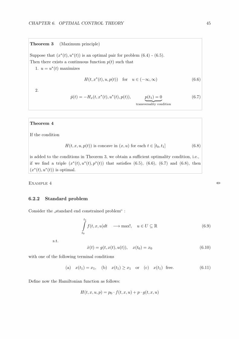
Theorem 5 (Maximum principle for standard end constraints)
Suppose that (x∗(t), u∗(t)) is an optimal pair for problem (6.9) - (6.11).Then there exist a continuous function p(t) and a number p0 ∈ {0, 1} such that for allt ∈ [t0, t1] we have (p0, p(t)) 6= (0, 0) and, moreover:
1. u = u∗(t) maximizes the Hamiltonian H(t, x∗(t), u, p(t)) w.r.t. u ∈ U , i.e.,
H(t, x∗(t), u, p(t)) ≤ H(t, x∗(t), u∗(t), p(t)) for all u ∈ U
2.p(t) = −Hx(t, x∗(t), u∗(t), p(t)) (6.12)
3. Corresponding to each of the terminal conditions (a), (b) and (c) in (6.11), there isa transversality condition on p(t1):(a’) no condition on p(t1)(b’) p(t1) ≥ 0 (with p(t1) = 0 if x∗(t1) > x1)(c’) p(t1) = 0
Theorem 6 (Mangasarian)
Suppose that (x∗(t), u∗(t)) is a feasible pair with the corresponding costate variable p(t)such that conditions 1. - 3. in Theorem 5 are satisfied with p0 = 1. Suppose furtherthat the control region U is convex and that H(t, x, u, p(t)) is concave in (x, u) for everyt ∈ [t0, t1].Then (x∗(t), u∗(t)) is an optimal pair.
General approach:
1. For each triple (t, x, p) maximize H(t, x, u, p) w.r.t. u ∈ U (often there exists a uniquemaximization point u = u(t, x, p)).
2. Insert this function into the differential equations (6.10) and (6.12) to obtain
x(t) = g(t, x, u(t, x(t), p(t)))
andp(t) = −Hx(t, x(t), u(t, x(t), p(t)))
(i.e., a system of two first-order differential equations) to determine x(t) and p(t).
3. Determine the constants in the general solution (x(t), p(t)) by combining the initial condi-tion x(t0) = x0 with the terminal conditions and transversality conditions.
=⇒ state variable x∗(t), corresponding control variable u∗(t) = u(t, x∗(t), p(t))
CHAPTER 6. OPTIMAL CONTROL THEORY 47
Remarks:
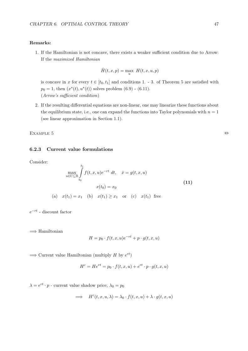
1. If the Hamiltonian is not concave, there exists a weaker sufficient condition due to Arrow:If the maximized Hamiltonian
H(t, x, p) = maxu
H(t, x, u, p)
is concave in x for every t ∈ [t0, t1] and conditions 1. - 3. of Theorem 5 are satisfied withp0 = 1, then (x∗(t), u∗(t)) solves problem (6.9) - (6.11).(Arrow’s sufficient condition)
2. If the resulting differential equations are non-linear, one may linearize these functions aboutthe equilibrium state, i.e., one can expand the functions into Taylor polynomials with n = 1
Theorem 7 (Maximum principle, current value formulation)
Suppose that (x∗(t), u∗(t)) is an optimal pair for problem (11) and let Hc be the currentvalue Hamiltonian.Then there exist a continuous function λ(t) and a number λ0 ∈ {0, 1} such that for allt ∈ [t0, t1] we have (λ0, λ(t)) 6= (0, 0) and, moreover:
1. u = u∗(t) maximizes Hc(t, x∗(t), u, λ(t)) for u ∈ U2.
λ(t)− rλ(t) = −∂Hc(t, x∗(t), u∗(t), λ(t))
∂x
3. The transversality conditions are:(a’) no condition on λ(t1)
Remark:The conditions in Theorem 7 are sufficient for optimality if λ0 = 1 and
Hc(t, x, u, λ(t)) is concave in (x, u) (Mangasarian)
or more generally
Hc(t, x, λ(t)) = maxu∈U
Hc(t, x, u, λ(t)) is concave in x (Arrow).
Example 6 /
Remark:If explicit solutions for the system of differential equations are not obtainable, a phase diagrammay be helpful.
Illustration: Phase diagram for example 6 /
Chapter 7
Applications to growth theory andmonetary economics
7.1 Some growth models
Example 1: Economic growth I /
Let
X = X(t) - national product at time tK = K(t) - capital stock at time tL = L(t) - number of workers (labor) at time t
and
X = A ·K1−α · Lα - Cobb-Douglas production functionK = s ·X - aggregate investment is proportional to outputL = L0 · eλt - labor force grows exponentially(A,α, s, L, λ > 0; 0 < α < 1).
Example 2: Economic growth II /
Let
X(t) - total domestic product per yearK(t) - capital stockσ - average productivity of capitals - savings rateH(t) = H0 · eµt (µ 6= s · σ) - net inflow of foreign investment per year at time t
49
CHAPTER 7. GROWTH THEORY AND MONETARY ECONOMICS 50
7.2 The Solow-Swan model
• neoclassical Solow-Swan model: model of long-run growth
• generalization of the model in Example 1 in Section 7.1
Assumptions and notations:
Y = Y (t) - (aggregate) output at time tK = K(t) - capital stock at time tL = L(t) - number of workers (labor) at time tF (K,L) - production function (assumption: constant returns to scale, i.e., F is homogeneous ofdegree 1)
=⇒ Y = F (K,L) or equivalently y = f(k), where
y = YL - output per worker
k = KL - capital stock per worker
C - consumptionc = C
L - consumption per worker
s - savings rate (0 < s < 1)
=⇒ C = (1− s)Y or equivalently c = (1− s)y
i - investment per worker
=⇒ y = c+ i = (1− s)y + i
=⇒ i = s · y = s · f(k)
Illustration: Output, investment and capital stock per worker /
δ - depreciation rate
Law of motion of capital stockk = s · f(k)︸ ︷︷ ︸
investment
− δk︸︷︷︸depreciation
equilibrium state k∗:k = 0 =⇒ s · f(k∗) = δk∗ (7.1)
Illustration: Equilibrium state /
CHAPTER 7. GROWTH THEORY AND MONETARY ECONOMICS 51
Golden rule level of capital accumulation
The government would choose an equilibrium state at which consumption is maximized. To alterthe equilibrium state, the government must change the savings rate s:
c = f(k)− s · f(k)
(7.1)=⇒ c = f(k∗)− δ · k∗ (at the equilibrium state k∗)
=⇒ necessary optimality condition for c −→ max!
f ′(k∗)− δ = 0 =⇒ f ′(k∗) = δ (7.2)
Using (7.1) and (7.2), we obtain:
s∗ · f(k) = f ′(k) · k =⇒ s∗ =f ′(k) · kf(k)
s∗ - savings rate, that maximizes consumption at the equilibrium state
Example 3 /
Introducing population growth
Let
λ = LL - growth rate of the labor force.
=⇒ equilibrium state k∗:s · f(k∗) = (δ + λ)k∗
Introducing technological progress
−→ technological progress results from increased efficiency E of labor
Let
g = EE - growth rate of efficiency of labor.
Y = F (K,L · E) =⇒ y = f
(K
L · E
)= f(k)
equilibrium state k∗:s · f(k∗) = (δ + λ+ g)k∗
CHAPTER 7. GROWTH THEORY AND MONETARY ECONOMICS 52
Interpretation:
At k∗ y and k are constant. Thus:
1. Since y = YL·E , L grows at rate λ, E grows at rate g
=⇒ Y must grow at rate λ+ g.
2. Since k = KL·E , L grows at rate λ, E grows at rate g