Michael J. Ostwald Research - Springer · 446 Michael J. Ostwald – The Mathematics of Spatial...

Michael J. Ostwald University of Newcastle

School of Architecture and Built Environment Faculty of Engineering and Built Environment

Callaghan, New South Wales 2398 AUSTRALIA

[email protected]

Keywords: Justified plan graph, graph theory, Space Syntax, mathematical analysis, plan

analysis

Research

The Mathematics of Spatial Configuration: Revisiting, Revising and Critiquing Justified Plan Graph Theory Abstract. The justified plan graph (JPG) was the first practical analytical method developed as part of the theory of Space Syntax, which purported to provide a graphical, mathematical and associated theoretical model for analysing the spatial configuration of buildings. In spite of early interest, in recent years relatively little research using this method has been published, perhaps because the JPG method is rarely explained in its totality and when it is, the descriptions are often inconsistent or unclear. Although it is now embedded in several software programs and its use may be more widespread, it is no better understood and after processing there is a marked lack of consistency in how the results are interpreted. This paper provides a historical background for the development of the JPG and a discussion of its conceptual or theoretical origins, followed by a “worked example” of the mathematics of the JPG. In combination with the results for two further cases, the paper identifies some important interpretative limits in the method and uses the examples to explain its potential use in design analysis. Finally, the paper discusses how the consistent application of this method to sets of related buildings is likely to produce a more valuable, and statistically viable, basis for future work.

Introduction Developed primarily in the early 1980s in London, Space Syntax is the collective title

given to a number of theories, tools or techniques that seek to draw connections between spatial configurations and social effects. While originally established for the study of architecture, Space Syntax theory has since been applied to the analysis of urban space and it has become one of the major analytical methods available for studying historic settlement patterns. Despite sporadic criticism of both its philosophical and mathematical foundations, and ongoing debate about its application, it remains a powerful conceptual tool for the analysis of the built environment.

The essential works of Space Syntax are the Social Logic of Space [Hillier and Hanson 1984], Space is the Machine [Hillier 1995] and Decoding Houses and Homes [Hanson 1998]. These three books by Bill Hillier and Julienne Hanson, along with a large number of additional papers by Alan Penn and John Peponis, define the primary conceptual framework of the theory. That is, Space Syntax promotes a conceptual shift in understanding architecture wherein “dimensional” or “geographic” thinking is rejected in favour of “relational” or “topological” reasoning. This shift, which is further elaborated in the following sections of the present paper, relies on the process of translating architecturally defined space into a series of topological graphs that may be mathematically analysed (graph analysis) and then interpreted (graph theory) in terms of their architectural, urban, social or spatial characteristics.

Nexus Network Journal 13 (2011) 445–470 Nexus Network Journal – Vol. 13, No. 2, 2011 445 DOI 10.1007/s00004-011-0075-3; published online 9 June 2011© 2011 Kim Williams Books, Turin

446 Michael J. Ostwald – The Mathematics of Spatial Confi guration: Revisiting, Revising…

While Space Syntax researchers have developed a range of analytical processes and theories, the focus of the present paper is the “justified plan graph” (JPG). This method has been known by a number of titles including “planar graphs” [March and Steadman 1971: 242] and “plan morphology” [Steadman 1983: 209], and it has been described as producing either a “justified graph” or a “justified permeability graph” [Hanson 1998: 27, 247]. Alternatively, the method is sometimes presented as producing a “plan graph”, an “access graph” [Stevens 1990: 208] or a “justified access graph” [Shapiro 2005: 114]. Most recently, naming of the method has tended to return to the earlier, more general descriptors including “node analysis” and “connectivity graph analysis” [Manum 2009]. While Steadman [1983] provides different definitions for a plan graph and an access graph, the two concepts have been largely melded in subsequent use. To further complicate matters, Hillier and Hanson distinguish the syntactic analysis of urban settlements, which they call “alpha-analysis” [1984: 90] from the analysis of the interior, which they call “gamma-analysis” [1984: 147]. This means that the plan graph may also be described as a “gamma map” [1984: 147], an appellation which infers membership of a category (interior analysis) rather than a specific type of graph. For consistency, in the present paper the method is described as producing a “justified plan graph” (JPG).

The confusion surrounding the naming of this form of analysis may be one of many factors that have limited its application. Another reason is suggested by Dovey, who argues that the real problem is that “Hillier’s work is at times highly difficult to understand” [1999: 24]. With its often opaque language “of ‘distributed’ and ‘non-distributed’ structures which reveal ‘integration’ values measured by a formula for ‘relative asymmetry’” [1999: 25] the theory underlying the construction of JPGs is not easy to comprehend. Furthermore, the “evidence” for the method is typically presented “in the form of complex mathematical tables” [1999: 25] with little or no explanation of the origins of the values [Manum 2009]. Dovey is critical both of the lack of clarity of the mathematics underlying the theory and of the fact that as the opacity of the method grows, “so does the danger that such approaches may be … defended from everyday critique by their technical ‘difficulty’” [1999: 25].

It is at least partially true that no single, clear and concise explanation of the current state of the JPG method exists in any one publication.1 In a field that is still under development, albeit at a much slower pace than in the 1980s, it is not unusual to find that even the canonical works [Hillier and Hanson 1984; Hillier 1995; Hanson 1998] can no longer be considered as providing a complete and consistent explanation of JPG analysis or theory. What they do provide is a window into the state of JPG research at the time each book was written. Since then, explanations of JPG analysis have tended to be less consistent and are typically self-referential. As Klarqvist [1993] observes, they use a mix of nomenclature and often-unexplained variations of the key formulas. Conversely, some of the best descriptions of the JPG can be found in works which are either never cited as part of Space Syntax [Steadman 1983] or are critical of it [Osman and Suliman 1994]. Thus, while it is possible to construct a full and complete (if not consistent and transparent) explanation of the JPG method from published materials, it requires, as Dovey [1999] observes, an extensive investment of time and energy.

In response to this situation, the present paper provides a background to the rise of Space Syntax along with an explanation of the key theoretical concepts associated with graph theory and the JPG. Thereafter the paper is divided into two halves: the first on the mathematics of the JPG, or graph analysis, and the second on its visual and architectural interpretation, graph theory. In the first of these major sections a fully worked example of the mathematics of the JPG is offered along with a critical

Nexus Network Journal – Vol. 13, No. 2, 2011 447

commentary on each stage. Inspired by Hanson’s [1998] explanation of the theory, the paper proposes three similar hypothetical building plans as the focus, the first of which is the subject of the worked example (JPG analysis), while the latter two are central to the discussion of the interpretation of the results (JPG theory).

While it could be said that all of the stages of the JPG approach have been recorded in some form in previous research, the construction of a consistent mathematical and theoretical framing is the first aim of the present paper. As previously demonstrated, scholars have identified a serious need for such a description. The secondary intent of the paper is to balance the descriptive or analytical with the reflective or theoretical; it is apparent that even at its most advanced stage, there was widespread debate about the validity of the JPG method and the usefulness and meaning of its results. While the purpose of the present paper is neither to respond to past criticisms, nor to blindly repeat the standard answers of the Space Syntax movement, its commentary is informed by both of these dimensions. Finally, the paper concludes with a discussion of the need for the development and publication of consistently produced, statistically viable sets of JPG results. This process may, in turn, lead to the generation of a range of genotypes that can be used for benchmarking approaches to spatial configuration in architectural design.

Graph theory Graph theory is conventionally regarded as originating in the seventeenth-century

paradox of the Bridges of Königsberg: a mathematical puzzle about seven bridges separating four landmasses and a Knight’s desire to cross each bridge only once while moving in a continuous sequence [Harary 1960; Hopkins and Wilson 2004] (fig. 1). This problem was famously solved by Euler who, in 1735, removed all of the geographic and urban complexity from the puzzle to focus only on a diagram of four nodes (landforms) and seven connections (bridges) (fig. 2). Euler used this graphical method to prove that it wasn’t possible to complete the Knight’s desired journey for the particular set of spatial conditions.

Fig. 1. The geography of the Bridges of Königsberg, based on [March and Steadman 1971]

Fig. 2. A plan graph of the Bridges of Königsberg, based on [March and

Steadman 1971]

While isolated examples of graph theory may be found in nineteenth-century mathematics, it wasn’t until the 1960s and early 1970s that there was a growth in interest in the potential of graph theory to explain a variety of spatial and geographic phenomena [Harary 1969]. Moreover, at around this time graph theorists began to apply simple mathematical calculations to their node and line (or vertex and edge) diagrams to calculate the relative depth of these structures [Seppänen and Moore 1970; Taaffe and Gauthier 1973]. These same formulas provided the mathematical basis for Space Syntax


research a decade later and in the intervening years they were responsible for encouraging a range of mathematical applications in architecture. For example, having published a simple computational model of architectural design, Christopher Alexander [1964] soon developed a variation of graph theory to explain urban connectivity [1966] before combining graph theory and a rule-based grammar to define a pattern-based approach to design [Alexander et al. 1977]. However, within a few years of this publication Alexander rejected the mathematics of graph theory, preferring instead to seek geometric or relational systems in graphs.

Similarly, March and Steadman [1971] collaboratively developed the early stages of a syntactical model of form that drew on graph theory before later separately producing extrapolations of this idea [March 1976; Steadman 1973; 1983]. However, despite being inspired by graph theory, the work of March and Steadman soon developed a focus on architectural form and graph theory was less useful for that research direction. This view was reinforced by Stiny [1975] who, along with March and Steadman [1971], could be considered as having laid the foundations for both Shape Grammar analysis and Design Computing in architecture. This meant that by the 1980s the only architectural researchers to retain a serious interest in graph theory were Hillier, Hanson and their colleagues.

Form and space In 1984 Bill Hillier and Julienne Hanson argued that “[h]owever much we may

prefer to discuss architecture in terms of visual styles, its most far-reaching practical effects are not at the level of appearances at all, but at the level of space” [1984: ix]. For Hillier and Hanson space is the fundamental medium through which architects provide shelter, structure society and serve the basic needs of communities. This idea is emphatically expressed in Hillier’s adage, “space is the machine” [1995], the central maxim of Space Syntax theory. However, in order to understand Hillier and Hanson’s proposition it is first necessary to place it in context.

Critics and historians have traditionally defined architecture as the art and science of constructing form. Architectural form has shape, dimensionality and actual or intended physical properties [Gelernter 1995]. The particular way in which a form is modulated or moulded, in combination with its tectonic expression and underlying structure, is a reflection of the style of the architecture [Birkerts 1994]. As a result of the focus on form, texture and materiality, historians and critics have developed elaborate techniques for classifying architecture from various eras and for hypothesising the impact these buildings have on peoples’ physical and emotional responses. This focus on form as structure and as style is not surprising, given that the oldest definition of architecture, arising from Vitruvius, embraces works which exhibit suitable refinement in firmitas, utilitas and venustas , translated as either “soundness, utility and attractiveness” [Rowland and Howe 1999: 26] or as “firmness, commodity and delight” by Henry Wotton in 1624. Two of these three categories, firmness and delight, are directly tied to issues of form and are readily analysed and critiqued from this perspective. The third category, utility or commodity, has been less clearly defined. Vitruvius talks of utilitas in a design as facilitating “faultless, unimpeded use through the disposition of space” [Rowland and Howe 1999: 26]. Thus, the word “utility” suggests a degree of usefulness or functionality and the adjective “commodious” refers to things that are generous, capacious or accommodating. Both of these translations suggest a concern for spatial rather than formal properties. But what then is the relationship between space and form in architecture?


Ching describes the relationship between form and space as a “unity of opposites” [2007: 96]. He suggests that form in architecture refers to the “configuration or relative disposition of the lines or contours that delimit a figure” [2007: 34]. In contrast, space is that which is either enclosed by, or shaped by, form. Thus, a building delineates both the space it contains (its interior) and, to a lesser extent, the space in which it is contained (its site or context). Ching identifies the figure-ground plan as a rare example of a type of representation which privileges space over form: a visual device to encourage the eye to view the reciprocal relationship between solid and void. Architectural theories are conventionally focussed on form. From Pevsner’s [1936] celebration of symbolic architecture to Frampton’s [1995] call for a regional tectonic practice, form is central to our ethical or moral interpretation of design. Similarly, from Jencks and Baird’s [1969] meditations on semiotics to Pallasmaa’s [2005] phenomenology of place, architecture is read through its formal expression and the way in which the human body experiences or interprets that expression. All of these ways of viewing architecture are drawn from two of the three pillars of classical Vitruvian thought – firmness and delight. The final pillar, commodity, and especially insofar as it refers to spatial configuration, has had, in relative terms, little impact on the analysis of architectural history.

In order to overcome this deficit, Hillier and Hanson [1984] developed a theory of space without form. They argue that space may be empty, invisible and amorphous, but it does have two critical qualities, depreciable difference and permeability. The first of these qualities refers to the capacity to differentiate one space from any other, and the second refers to the way in which spaces are physically connected or configured. Another way of looking at the study of spatial configuration in isolation entails the rejection of two conventional geographic concerns, “the concept of location” and the “notion of distance” [Hillier and Hanson 1984: xii]. Neither of these properties or qualities is useful for understanding space as it is isolated from form. Instead, various “morphological qualities” [1984: xii], including the relationships between spaces and their relative permeability or complexity, can be studied. In practice one of the first methods adopted for the analysis of “non-geographic” space, the JPG, borrowed from the mathematics of graph theory to propose an alternative way of viewing an architectural plan. The construction of a JPG involves an inversion of the hierarchy implicit in this conventional representational schema. The JPG emphasises, at the expense of all other information, the number of spaces and the connections between them.

Developing the JPG

In Space Syntax the first step in the process is typically the production of a “convex map”. The convex map serves to translate an architectural or urban plan into a diagram that reflects the configuration of selected properties of that plan. Regardless of whether researchers are interested in plan configuration, axial mapping or visual link identification, this is a necessary transition between the architectural or urban plan and the production of a graph [Turner et al. 2001]. As Hillier and Tzortzi explain,

[s]patial layouts are first represented as a pattern of convex spaces, lines, or fields of view covering the layout (or … some combination of them), and then calculations are made of the configurational relations between each spatial element and all, or some, others [2006: 285].


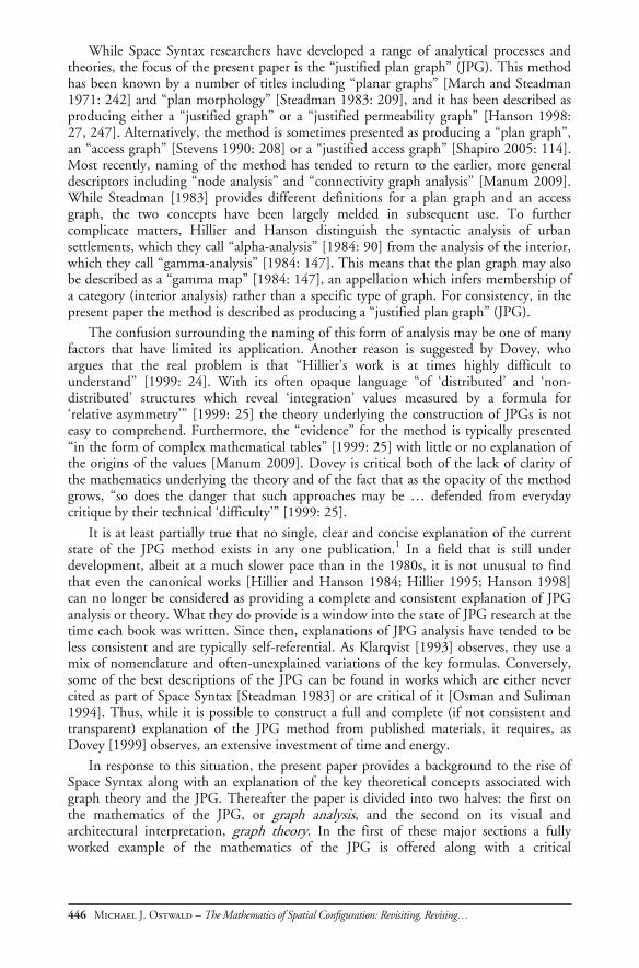
Fig. 3. Villa Alpha, cut-away view of the Architectural Plan

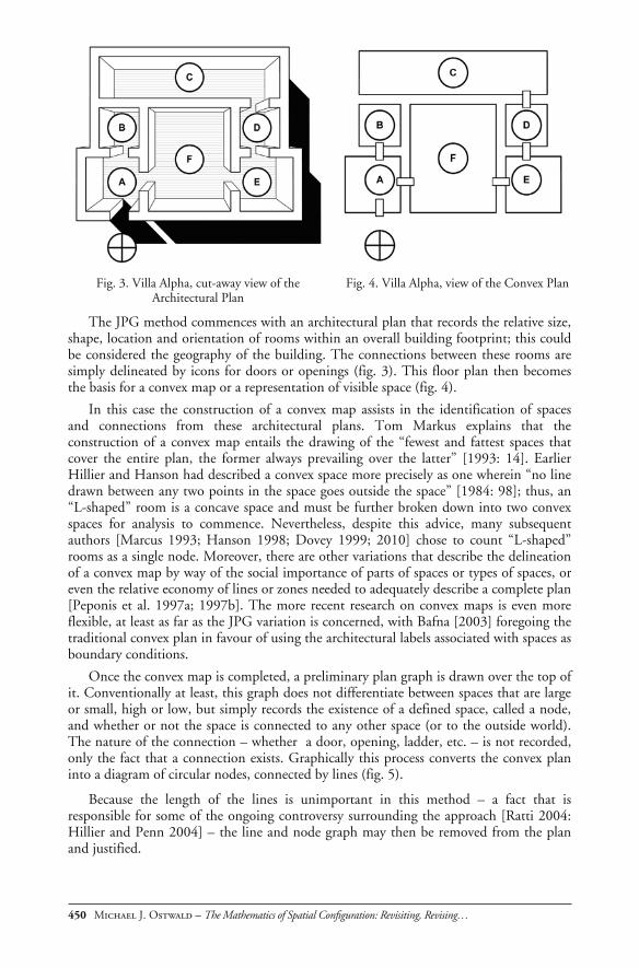
Fig. 4. Villa Alpha, view of the Convex Plan

The JPG method commences with an architectural plan that records the relative size, shape, location and orientation of rooms within an overall building footprint; this could be considered the geography of the building. The connections between these rooms are simply delineated by icons for doors or openings (fig. 3). This floor plan then becomes the basis for a convex map or a representation of visible space (fig. 4).

In this case the construction of a convex map assists in the identification of spaces and connections from these architectural plans. Tom Markus explains that the construction of a convex map entails the drawing of the “fewest and fattest spaces that cover the entire plan, the former always prevailing over the latter” [1993: 14]. Earlier Hillier and Hanson had described a convex space more precisely as one wherein “no line drawn between any two points in the space goes outside the space” [1984: 98]; thus, an “L-shaped” room is a concave space and must be further broken down into two convex spaces for analysis to commence. Nevertheless, despite this advice, many subsequent authors [Marcus 1993; Hanson 1998; Dovey 1999; 2010] chose to count “L-shaped” rooms as a single node. Moreover, there are other variations that describe the delineation of a convex map by way of the social importance of parts of spaces or types of spaces, or even the relative economy of lines or zones needed to adequately describe a complete plan [Peponis et al. 1997a; 1997b]. The more recent research on convex maps is even more flexible, at least as far as the JPG variation is concerned, with Bafna [2003] foregoing the traditional convex plan in favour of using the architectural labels associated with spaces as boundary conditions.

Once the convex map is completed, a preliminary plan graph is drawn over the top of it. Conventionally at least, this graph does not differentiate between spaces that are large or small, high or low, but simply records the existence of a defined space, called a node, and whether or not the space is connected to any other space (or to the outside world). The nature of the connection – whether a door, opening, ladder, etc. – is not recorded, only the fact that a connection exists. Graphically this process converts the convex plan into a diagram of circular nodes, connected by lines (fig. 5).

Because the length of the lines is unimportant in this method – a fact that is responsible for some of the ongoing controversy surrounding the approach [Ratti 2004: Hillier and Penn 2004] – the line and node graph may then be removed from the plan and justified.


Fig. 5. Villa Alpha, view of the Plan Graph

Fig. 6. Villa Alpha, view of Justified Plan Graph (exterior carrier)

The word “justified” refers to the process of arranging the graph by the relative depth of nodes from a given starting point generally known as the “carrier” or “root” space [Klarqvist 1993]. Thus, the JPG is constructed around a series of horizontal, dotted lines, numbered consecutively from 0, the lowest line. Each dotted line represents a level of separation between rooms. The carrier node, often the outside world, is located on the lowest line on the chart (line 0). Those spaces that are directly connected to the carrier are located on the line above (line 1). Further spaces directly connected to those on line 1 are placed on line 2, and so on. The exterior is represented in the JPG as a crossed circle (or in text as ) while other nodes are given letters (or, less often, numbers) that can be keyed to particular programmatic functions (fig. 6). Once a JPG is produced it is possible to analyse it mathematically.

JPG analysis: a worked example

While the previous section described the development of the JPG from a convex map, the present section explains the mathematics of the JPG using the same hypothetical building, the Villa Alpha, as an example. The process for mathematically analysing a building by using a JPG typically involves at least the first five steps, and possibly all nine, of the sequence that follows.

Step 1. The total number K of nodes or spaces in a set is determined. The depth of each node, relative to a carrier, is also calculated; that is, how many levels L deep in the JPG the node is. The number of nodes nx at a given level and for a given carrier is also recorded. The number of levels is counted in the JPG from the lowest, the carrier at 0, spaces directly connected to the carrier at 1, and so on. For example, for the Villa Alpha, K = 7 (that is, there are 7 nodes: , A, B, C, D, E, F) and there are 6 levels (0, 1, 2, 3, 4, 5) when arrayed with as carrier. Thus, for the JPG of the Villa Alpha with the exterior as carrier, the L value for node E = 3 (fig. 6).


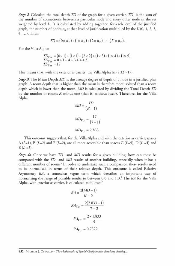
Step 2. Calculate the total depth TD of the graph for a given carrier. TD is the sum of the number of connections between a particular node and every other node in the set weighted by level L. It is calculated by adding together, for each level of the justified graph, the number of nodes nx at that level of justification multiplied by the L (0, 1, 2, 3, 4, …). Thus:

xxxx nXnnnTD 210 .

For the Villa Alpha:

17543410

514131221110

VVV

TDTDTD

.

This means that, with the exterior as carrier, the Villa Alpha has a TD=17.

Step 3. The Mean Depth MD is the average degree of depth of a node in a justified plan graph. A room depth that is higher than the mean is therefore more isolated than a room depth which is lower than the mean. MD is calculated by dividing the Total Depth TD by the number of rooms K minus one (that is, without itself). Therefore, for the Villa Alpha:

. 833.2

1717

1

V

V

MD

MD

KTDMD

This outcome suggests that, for the Villa Alpha and with the exterior as carrier, spaces A (L=1), B (L=2) and F (L=2), are all more accessible than spaces C (L=5), D (L =4) and E (L =3).

Step 4a. Once we have TD and MD results for a given building, how can these be compared with the TD and MD results of another building, especially when it has a different number of rooms? In order to undertake such a comparison these results need to be normalised in terms of their relative depth. This outcome is called Relative Asymmetry RA, a somewhat vague term which describes an important way of normalising the range of possible results to between 0.0 and 1.0.2 The RA for the Villa Alpha, with exterior as carrier, is calculated as follows:3

271833.22

212

VRA

KMDRA

.7322.0

5833.12

V

V

RA

RA


When this calculation is repeated for all of the carriers for the Villa Alpha a sequence can be constructed from the most isolated node to the least isolated: “most isolated” > C (0.93), (0.73), B (0.73), D (0.60), E (0.40), A (0.40) and F (0.33) > least isolated.

Because the RA results are normalised to a range between 0.0 and 1.0, RA results for nodes in different buildings may be usefully compared, although the veracity of this comparison is reduced if the K values (total number of spaces) become too dissimilar. Thus, the RA values of two houses, each with 9 rooms, may be directly compared. The RA values for two houses with, say, K values of 9 and 11 might also be compared, but the larger the differential between the two K values the less valid the comparison. In order to make a valid comparison between different size sets, an idealised benchmark must be used. For a comparative variation suitable for unequal K values see Step 4b.

Step 5a. If the RA for a carrier space is a reflection of its relative isolation, then the degree of integration i of that node in the JPG can be calculated by taking its reciprocal. Therefore, the integration value for the exterior space of the Villa Alpha may be calculated as follows:

. 364.1

733.01

1

V

V

i

iRA

i

Once again, while this value is relatively meaningless in isolation, it is more informative when compared with either the rest of the building it is part of, or alternatively, an ideally distributed benchmark plan. In the first instance, for the Villa Alpha a comparison between i results for each room reveals a hierarchy of space from least integrated to most integrated as follows: least integrated < C (1.07), (1.36), B (1.36), D (1.66), E (2.50), A (2.50) and F (3.00) < most integrated. Because of the reciprocal relationship between i and RA, this is simply the reverse order of the previous result recorded in Step 4a. However, whereas RA results were limited to a range between 0.0 and 1.0, i results start at 1.0 and have no upper limit. Nevertheless, in order to use this data to construct a comparison with a building of a radically different size, then a comparison must be constructed against an optimal benchmark (see Step 5b).

Step 4b. This is an alternative to Step 4a which was focused on Relative Asymmetry RA. Real Relative Asymmetry RRA describes the degree of isolation or depth of a node not only in comparison to its complete set of results but also in comparison with a suitably scaled and idealised benchmark configuration. Thus, while RA results are effectively normalised or standardised against a set range of results (0-1), RRA results are relativised against a benchmark configuration.

RRA results are useful for comparisons between buildings with radically different K values because, as buildings grow in configurational complexity and scale, their RA values typically fall. This outcome is a result of practical circumstances, rather than mathematical functions, but it does tend to confirm the importance of the RRA analytical process. Despite this, many contemporary scholars [Shapiro 2005: Thayler 2005; Manum et al. 2005] ignore RRA in favour of RA because they are not convinced by the logic of Hillier’s and Hanson’s method [Krüger 1989; Asami et al. 2003: Thayler 2005].


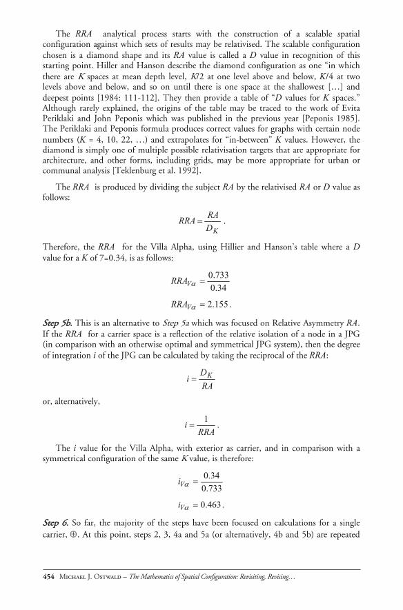
The RRA analytical process starts with the construction of a scalable spatial configuration against which sets of results may be relativised. The scalable configuration chosen is a diamond shape and its RA value is called a D value in recognition of this starting point. Hiller and Hanson describe the diamond configuration as one “in which there are K spaces at mean depth level, K/2 at one level above and below, K/4 at two levels above and below, and so on until there is one space at the shallowest […] and deepest points [1984: 111-112]. They then provide a table of “D values for K spaces.” Although rarely explained, the origins of the table may be traced to the work of Evita Periklaki and John Peponis which was published in the previous year [Peponis 1985]. The Periklaki and Peponis formula produces correct values for graphs with certain node numbers (K = 4, 10, 22, …) and extrapolates for “in-between” K values. However, the diamond is simply one of multiple possible relativisation targets that are appropriate for architecture, and other forms, including grids, may be more appropriate for urban or communal analysis [Teklenburg et al. 1992].

The RRA is produced by dividing the subject RA by the relativised RA or D value as follows:

KDRARRA .

Therefore, the RRA for the Villa Alpha, using Hillier and Hanson’s table where a D value for a K of 7=0.34, is as follows:

. 155.2

34.0733.0

V

V

RRA

RRA

Step 5b. This is an alternative to Step 5a which was focused on Relative Asymmetry RA. If the RRA for a carrier space is a reflection of the relative isolation of a node in a JPG (in comparison with an otherwise optimal and symmetrical JPG system), then the degree of integration i of the JPG can be calculated by taking the reciprocal of the RRA:

RAD

i K

or, alternatively,

RRAi 1

.

The i value for the Villa Alpha, with exterior as carrier, and in comparison with a symmetrical configuration of the same K value, is therefore:

. 463.0

733.034.0

V

V

i

i

Step 6. So far, the majority of the steps have been focused on calculations for a single carrier, . At this point, steps 2, 3, 4a and 5a (or alternatively, 4b and 5b) are repeated


for each other potential carrier producing a “distance data” table (table 1). In this table for the Villa Alpha, the top horizontal row of italic cells starting from 0 and (i.e. below the column titles) record the set of results in the previous steps in this paper for the exterior carrier graph. Repeating this process for each node as carrier fills the remainder of the cells. The simplest way to do this is to produce the distance matrix in the chart, where each of the six spaces and the exterior (making seven) are placed in a matrix opposite the same space, and the number of connections needed to pass from each space to each other space is recorded. Thus, there will always be a set of cells with 0 in them where the matrix crosses. Finally, the mean results for the Villa Alpha, for TD, MD, RA and i are recorded in the table.

# Space V A B F E D C TDn MDn RA i 0 0 1 2 2 3 4 5 17 2.83 0.73 1.36 1 A 1 0 1 1 2 3 4 12 2.00 0.40 2.50 2 B 2 1 0 2 3 4 5 17 2.83 0.73 1.36 3 F 2 1 2 0 1 2 3 11 1.83 0.33 3.00 4 E 3 2 3 1 0 1 2 12 2.00 0.40 2.50 5 D 4 3 4 2 1 0 1 15 2.50 0.60 1.66 6 C 5 4 5 3 2 1 0 20 3.33 0.93 1.07 Mean 14.85 2.47 0.59 1.92

Table 1. Distance data table for Villa Alpha

Step 7. The Control Value CV of a JPG is typically described as being a reflection of the degree of influence exerted by a space in a network [Jiang et al. 2000: Xinqi et al. 2008]. For example, Klarqvist describes it as “a dynamic local measure” which determines “the degree to which a space controls access to its immediate neighbours” [1993: 11]. Actually, any node has the potential to be a site of control and certain spatial configurations may increase that potential, but otherwise the CV has relatively little to do with power or control. The problem with the CV is that too often scholars have attempted to explain its value within space or architecture without first asking: What is the mathematics doing in this equation? Peponis [1985] offers one of the early definitions of the CV formula wherein the control value of a given point a is determined by the following formula:

1,

1

baD bValaCV

In this formula Val(b) is the number of connections to a point, b.

If the CV equation and its operations are examined, the closest explanation for what it actually measures is offered by Asami’s team who propose that control must be “thought of as a measure of relative strength … in ‘pulling’ the potential [of the system] from its immediate neighbours” [2003: 48.6]. While this is reasonably close to the machinations of the formula, there is a notion in network theory entitled “distributed equilibrium” that also closely approximates the actual meaning of CV. Assume that a network has “capacity” of some sort and that without outside influence, this network will strive for equilibrium by automatically passing that capacity from one node equally to all adjacent nodes in the system (but no further and not back again). Once all of the capacity in the system has been simultaneously divided amongst its immediate neighbouring nodes in this way, the system will have achieved a state of equilibrium through the controlled, but unequal, distribution of its capacity. The difference between


nodes in this balanced state with more or less capacity is simply a factor of adjacent network configuration. Viewed in this way the CV value should be thought of as signifying sites of attraction, “pulling” potential or capacity, like whirlpools that retain their position in a stream.

Jason Shapiro describes the construction of the CV value as beginning with “counting the number of neighbours of each space” in the JPG, that is, “the spaces with which it has a direct connection”; this is called the NCn value. Then, “[e]ach space gives to its neighbours a value equal to 1/n of its ‘control’” [Shapiro 2005: 52]. The distributed or shared value of each node is known as CVe : thus, CVe = 1/NCn. Once the complete set of CVe values have been shared across the JPG, then the CV value for each node can be calculated. Calculating CV values therefore requires a holistic approach that methodically traces where every node is influenced by every connection it has. Thus, in the case of the Villa Alpha the following are three example calculations of CV values.

In the first example, Space has only one connection, space A, so it must distribute 1/1 or 1 CVe to the space it is connected to leaving it with an interim CV of 0. However, space A is connected to three spaces including and so it must distribute 1/3 or 0.33 CVe to each of these spaces. Thus, the CV for is 0+0.33=0.33. In the second example, the CV for space A is calculated by taking 1/n for each of spaces (1/1 = 1), B (1/1 = 1) and F (1/2 = 0.5). Therefore, the CV for space A is (1+1+0.5) = 2.50. Finally, the CV for space B is calculated by determining how many connections it has (NCn=1) and placing that in the formula CVe = 1/NCn, which produces a CVe = 1. Thus space B distributes its CVe of 1 to space A, leaving it with an interim CV value of 0. However, space A also distributes its CVe three ways including to B, passing a CVe of 0.33 back to B, giving space B a total CV result of 0.33.

The complete set of NCn, CVe and CV results for the Villa Alpha are contained in table 2. They reveal that room A, with a CV of 2.5 is by far the space with the greatest natural attraction, followed by room D, with a CV = 1.5. Shapiro [2005] suggests that control values above 1.00 are considered relatively high and typically define rooms that permit or enable access. Certainly room A is a pivotal space from the point of view of access and security, but room D (the second highest) has none of these qualities. This is why the simple definition of a CV value as pertaining to control is less convincing than seeing it as a site of natural influence or even better of natural congregation. For Shapiro, values below 1.00 “have only weak control over adjacent spaces” [2005, 52]. If this was true, then in the Villa Alpha, nodes , B and C – all of which are terminating branches in the JPG – would have amongst the lowest capacities to exert influence over other nodes. In the case of B and C this may be true, but it is less convincing for .

# Space V A B F E D C NCn CVe CV 0 0 1 0 0 0 0 0 1.00 1.00 0.33 1 A 1 0 1 1 0 0 0 3.00 0.33 2.50 2 B 0 1 0 0 0 0 0 1.00 1.00 0.33 3 F 0 1 0 0 1 0 0 2.00 0.50 0.83 4 E 0 0 0 1 0 1 0 2.00 0.50 1.00 5 D 0 0 0 0 1 0 1 2.00 0.50 1.50 6 C 0 0 0 0 0 1 0 1.00 1.00 0.50

Table 2. Connection Data Table for the Villa Alpha


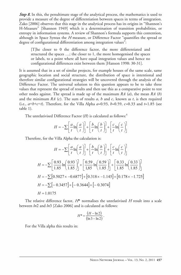
Step 8. In this, the penultimate stage of the analytical process, the mathematics is used to provide a measure of the degree of differentiation between spaces in terms of integration. Zako [2006] observes that this stage in the analytical process has its origins in “Shannon’s H-Measure” [Shannon 1949] which is a determination of transition probabilities, or entropy in information systems. A review of Shannon’s formula supports this contention, although in Space Syntax the H measure, or Difference Factor “quantifies the spread or degree of configurational differentiation among integration values”:

[T]he closer to 0 the difference factor, the more differentiated and structured the spaces …; the closer to 1, the more homogenised the spaces or labels, to a point where all have equal integration values and hence no configurational differences exist between them [Hanson 1998: 30-31].

It is assumed that in a set of similar projects, for example houses of the same scale, same geographic location and social structure, the distribution of space is intentional and therefore similar configurational strategies will be uncovered through the analysis of the Difference Factor. The universal solution to this question appears to be to take three values that represent the spread of results and then use this as a comparative point to test other nodes against. The spread is made up of the maximum RA (a), the mean RA (b) and the minimum RA (c). The sum of results a, b and c, known as t, is then required (i.e., a+b+c=t). Therefore, for the Villa Alpha a=0.93, b=0.59, c=0.33 and t=1.85 (see table 1).

The unrelativised Difference Factor (H) is calculated as follows:4

tc

tc

tb

tb

ta

taH lnlnln

Therefore, for the Villa Alpha the calculation is:

tc

tc

tb

tb

ta

taH lnlnln

0175.1

3074.03644.03457.0

725.1178.0145.1318.06877.05027.0

85.133.0ln

85.133.0

85.159.0ln

85,159.0

85.193.0ln

85.193.0

H

H

H

H

The relative difference factor, H* normalises the unrelativised H result into a scale between ln2 and ln3 [Zako 2006] and is calculated as follows:

2ln3ln2ln* HH .

For the Villa alpha this results in:


. 711.0*

4056.03245.0*

693.00986.1693.00175.1*

H

H

H

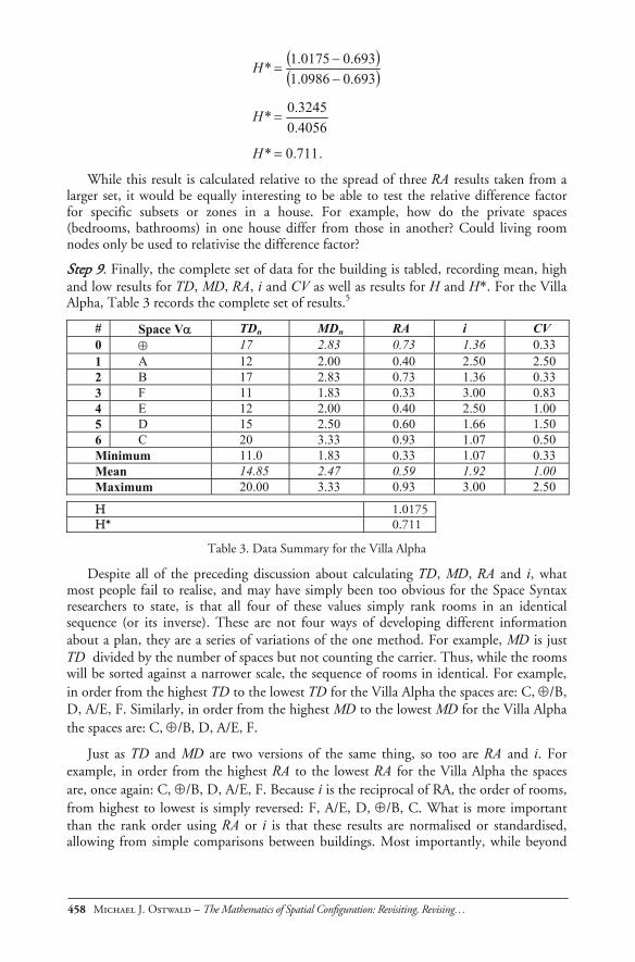
While this result is calculated relative to the spread of three RA results taken from a larger set, it would be equally interesting to be able to test the relative difference factor for specific subsets or zones in a house. For example, how do the private spaces (bedrooms, bathrooms) in one house differ from those in another? Could living room nodes only be used to relativise the difference factor?

Step 9. Finally, the complete set of data for the building is tabled, recording mean, high and low results for TD, MD, RA, i and CV as well as results for H and H*. For the Villa Alpha, Table 3 records the complete set of results.5

# Space V TDn MDn RA i CV 0 17 2.83 0.73 1.36 0.33 1 A 12 2.00 0.40 2.50 2.50 2 B 17 2.83 0.73 1.36 0.33 3 F 11 1.83 0.33 3.00 0.83 4 E 12 2.00 0.40 2.50 1.00 5 D 15 2.50 0.60 1.66 1.50 6 C 20 3.33 0.93 1.07 0.50 Minimum 11.0 1.83 0.33 1.07 0.33 Mean 14.85 2.47 0.59 1.92 1.00 Maximum 20.00 3.33 0.93 3.00 2.50

H 1.0175 H* 0.711

Table 3. Data Summary for the Villa Alpha

Despite all of the preceding discussion about calculating TD, MD, RA and i, what most people fail to realise, and may have simply been too obvious for the Space Syntax researchers to state, is that all four of these values simply rank rooms in an identical sequence (or its inverse). These are not four ways of developing different information about a plan, they are a series of variations of the one method. For example, MD is just TD divided by the number of spaces but not counting the carrier. Thus, while the rooms will be sorted against a narrower scale, the sequence of rooms in identical. For example, in order from the highest TD to the lowest TD for the Villa Alpha the spaces are: C, /B, D, A/E, F. Similarly, in order from the highest MD to the lowest MD for the Villa Alpha the spaces are: C, /B, D, A/E, F.

Just as TD and MD are two versions of the same thing, so too are RA and i. For example, in order from the highest RA to the lowest RA for the Villa Alpha the spaces are, once again: C, /B, D, A/E, F. Because i is the reciprocal of RA, the order of rooms, from highest to lowest is simply reversed: F, A/E, D, /B, C. What is more important than the rank order using RA or i is that these results are normalised or standardised, allowing from simple comparisons between buildings. Most importantly, while beyond


the scope of the present paper, in complex systems it has become increasingly important to be able to study subsets of a larger group. This could be thought of as the isolation of certain levels or distances, typically called a “radius”, and this requires the type of relativisation of data that the RA and i results produce. Thus, while in one sense they do not provide any new information about the relative integration of various rooms in a plan, they have the potential, and especially in large sets, to be used for different analytical purposes [Haq 2003].

Of all of the mathematical results, the CV method produces something slightly different. In order from highest CV to lowest CV, for the Villa Alpha, the rooms are: A, D, E, F, C, B/ . This result has some similarities to the way the i results broadly partition spaces, but they subtly shift the balance to signify a different type of importance: pulling power rather than integration.

JPG theory: diagrammatic analysis

Having seen how the JPG analysis is undertaken mathematically, it is also possible to interpret a JPG strictly as a diagram, that is, without mathematical support [Marcus 1993; Hanson 1998; Dovey 1999; 2010]. In order to explain this type of diagramatic analysis, let us add two additional hypothetical Villas, Beta (V ) (fig. 7) and Gamma (V ) (fig. 8) to the previously introduced Villa Alpha (V ).

Each of these three Villas possesses the same building footprint and the same number of rooms. The sizes of rooms and relative locations of each are also identical. Thus, from a geographic or geospatial perspective these buildings are largely identical. However, the way in which rooms are connected differs in each Villa, changing the spatial morphology in terms of permeability and depth. For example, consider a JPG, with the exterior as carrier, for each of the three villas. From this perspective it quickly becomes apparent that despite similar architectural plans, the spatial configuration present in the plan, including the degree of connectivity and depth, varies greatly (figs. 6, 9 and 10).

Fig. 7. Villa Beta, plan Fig. 8. Villa Gamma, plan


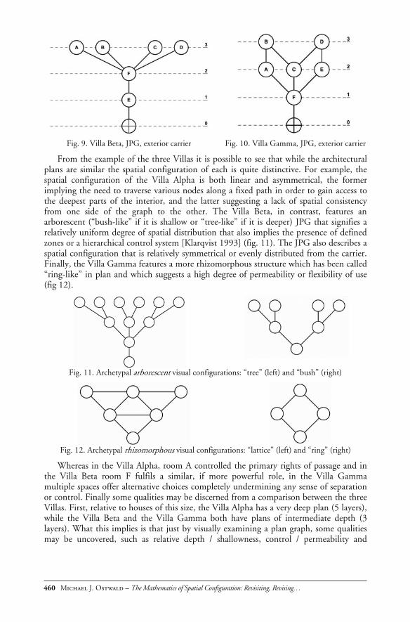
Fig. 9. Villa Beta, JPG, exterior carrier Fig. 10. Villa Gamma, JPG, exterior carrier

From the example of the three Villas it is possible to see that while the architectural plans are similar the spatial configuration of each is quite distinctive. For example, the spatial configuration of the Villa Alpha is both linear and asymmetrical, the former implying the need to traverse various nodes along a fixed path in order to gain access to the deepest parts of the interior, and the latter suggesting a lack of spatial consistency from one side of the graph to the other. The Villa Beta, in contrast, features an arborescent (“bush-like” if it is shallow or “tree-like” if it is deeper) JPG that signifies a relatively uniform degree of spatial distribution that also implies the presence of defined zones or a hierarchical control system [Klarqvist 1993] (fig. 11). The JPG also describes a spatial configuration that is relatively symmetrical or evenly distributed from the carrier. Finally, the Villa Gamma features a more rhizomorphous structure which has been called “ring-like” in plan and which suggests a high degree of permeability or flexibility of use (fig 12).

Fig. 11. Archetypal arborescent visual configurations: “tree” (left) and “bush” (right)

Fig. 12. Archetypal rhizomorphous visual configurations: “lattice” (left) and “ring” (right)

Whereas in the Villa Alpha, room A controlled the primary rights of passage and in the Villa Beta room F fulfils a similar, if more powerful role, in the Villa Gamma multiple spaces offer alternative choices completely undermining any sense of separation or control. Finally some qualities may be discerned from a comparison between the three Villas. First, relative to houses of this size, the Villa Alpha has a very deep plan (5 layers), while the Villa Beta and the Villa Gamma both have plans of intermediate depth (3 layers). What this implies is that just by visually examining a plan graph, some qualities may be uncovered, such as relative depth / shallowness, control / permeability and


symmetry / asymmetry. The first two of these categories have been used for the graphic analysis of power structures implicit in a range of institutional buildings [Marcus 1987; 1988; 1993; Dovey 1999; 2010].

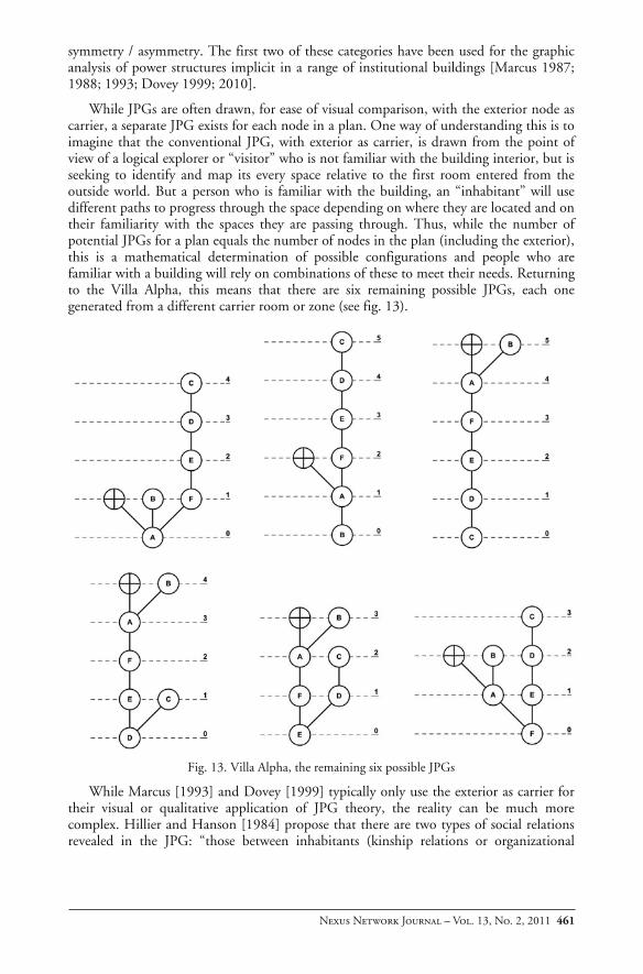
While JPGs are often drawn, for ease of visual comparison, with the exterior node as carrier, a separate JPG exists for each node in a plan. One way of understanding this is to imagine that the conventional JPG, with exterior as carrier, is drawn from the point of view of a logical explorer or “visitor” who is not familiar with the building interior, but is seeking to identify and map its every space relative to the first room entered from the outside world. But a person who is familiar with the building, an “inhabitant” will use different paths to progress through the space depending on where they are located and on their familiarity with the spaces they are passing through. Thus, while the number of potential JPGs for a plan equals the number of nodes in the plan (including the exterior), this is a mathematical determination of possible configurations and people who are familiar with a building will rely on combinations of these to meet their needs. Returning to the Villa Alpha, this means that there are six remaining possible JPGs, each one generated from a different carrier room or zone (see fig. 13).

Fig. 13. Villa Alpha, the remaining six possible JPGs

While Marcus [1993] and Dovey [1999] typically only use the exterior as carrier for their visual or qualitative application of JPG theory, the reality can be much more complex. Hillier and Hanson [1984] propose that there are two types of social relations revealed in the JPG: “those between inhabitants (kinship relations or organizational


hierarchies) and those between inhabitants and visitors” [Dovey 1999, 22]. Inhabitant-visitor relations can be reasonably well represented in a JPG with the exterior as carrier, but inhabitant-inhabitant relations are more complex and require consideration of multiple additional JPGs. For example a close review of the other six JPGs for the Villa Alpha shows that while, from the point of view of a visitor (carrier , fig. 6) the plan is linear and controlling, from the point of view of an inhabitant (carriers E or F, fig. 13) the plan is less linear, less deep and more symmetrical. This might suggest a somewhat defensive approach to visitors (or heightened desire for privacy), but a more balanced approach to inhabitation. The reality that multiple, parallel interpretations of the JPGs for a given building are possible, is often forgotten in graphical analysis; this fact can have significant analytical consequences. This is why, despite the usefulness of the JPG as a qualitative or visual tool, a more quantitative, mathematical approach is valuable.

JPG Theory: Interpretation and Discussion

Khadiga Osman and Mamoun Suliman argue that while the “analytical procedure of the [JPG] method is simple, objective, and replicable, the interpretation process of the numerical results remains complex, subjective and … controversial” [1994: 190]. Edmund Leach [1978] similarly suggests that while the mathematics may be used to make simple distinctions, the bigger question remains: What does this really say about social patterns in space? In this, the penultimate section of the paper, an attempt is made to use JPG theory to interpret the analytical or mathematical results recorded in the previous section for the Villa Alpha (Table 3) along with the results for the Villas Beta (Table 4) and Gamma (Table 5). The purpose of this comparison is to test whether the mathematical results, and their standard or anticipated interpretation, are supported by a simple comparison with two different spatial configurations of the same size K.

Starting with the depth of space TD results and excluding the exterior: for the Villa Alpha the deepest space, C, has a TD of 20; for the Villa Beta the deepest spaces, A, B, C and D have a TD of 12; and for the Villa Gamma, the deepest spaces, B or D have a TD of 12. This suggests that the plan with the deepest room is Alpha and that Beta and Gamma each have multiple spaces of similar depth, although overall less than Alpha. This certainly aligns with a common sense reading of the plans but it is also apparent that Beta and Gamma, despite having the same highest level of TD, are also quite different. Thus it may be more informative to calculate the mean TD results: TD V = 14.85, TD V = 11.42, TD V = 10.85. Given the same K values for each of the dwellings (that is, they all have the same number of spaces) it is not surprising that the degree of difference is reduced when the average weighted depth for the spatial configuration is determined. Thus mean MD for the villas is as follows: MDV = 2.47, MDV = 1.90, MDV = 1.80. Thus, the plan of Villa Beta is slightly deeper on average than the plan for the Villa Gamma.

So far, all of this is in accord with the anticipated results and the standard reading of the architectural qualities of such spaces. The question of what these results are useful for is slightly more perplexing. Certainly by identifying the average or mean result for some quality in a system it is immediately possible to classify nodes into “above” or “below” average (in this case depth). While of only minimal interest in the case of the three villas, it can be a useful quantity to know for larger buildings; for example, Hanson [1998] uses the JPG method to examine Bearwood Hall (c1865), an English manor house with 134 rooms.


# Space V TDn MDn RA i CV 0 15 2.50 0.60 1.66 0.50 1 F 7 1.16 0.06 15.00 4.50 2 A 12 2.00 0.40 2.50 0.20 3 B 12 2.00 0.40 2.50 0.20 4 C 12 2.00 0.40 2.50 0.20 5 D 12 2.00 0.40 2.50 0.20 6 E 10 1.66 0.26 3.75 1.20 Minimum 7.00 1.16 0.06 1.66 0.20 Mean 11.42 1.90 0.36 4.34 1.00 Maximum 15.00 2.50 0.60 15.00 4.50

H 0.766 H* 0.181

Table 4. Data Summary for the Villa Beta

# Space V TDn MDn RA i CV 0 13 2.16 0.46 2.14 0.25 1 F 8 1.33 0.13 7.50 2.33 2 A 11 1.83 0.33 3.00 0.75 3 C 9 1.50 0.20 5.00 1.25 4 E 11 1.83 0.33 3.00 0.75 5 B 12 2.00 0.40 2.50 0.83 6 D 12 2.00 0.40 2.50 0.83 Minimum 8.00 1.33 0.13 2.14 0.25 Mean 10.85 1.80 0.32 3.66 1.00 Maximum 13.00 2.16 0.46 7.50 2.33

H 0.99 H* 0.73

Table 5. Data Summary for the Villa Gamma

Putting aside this problem for the present, according to the theory of Hillier and Hanson [1984], a perfect shallow and symmetrical composition should have an RA close to 0.00, while a perfectly linear, enfilade structure should have an RA closer to 1.00. The Villa Alpha is mostly linear, with one deliberate variation and its mean result,

59.0VRA , which is closer to a value of 1 (a linear structure) seems to confirm this.

The Villa Beta is a relatively shallow and symmetrical structure. Only the presence of the vestibule spaces, E and F, removes the distribution of nodes from an ideal structure by adding two levels of depth; this leads to a mean RAV = 0.36. This result is closer to 0 (shallow and distributed) than to 1 (linear) once again supporting, albeit in an abstract way, the standard theoretical interpretation. Finally, the Villa Gamma has the lowest mean result, 32.0VRA , which implies it is the most shallow of the plans, but only by

a small margin.

The reciprocal of the RA is i : the integration dimension that is central to so much analysis using the JPG method [Shapiro 2005]. i is typically used to identify spaces, or sequences of spaces, that are pivotal to a spatial configuration and those which are not. The use of i to rank a set of rooms is also a special type of data set. As Sonit Bafna records, the “ranking of programmatic labelled spaces according to their mean depth


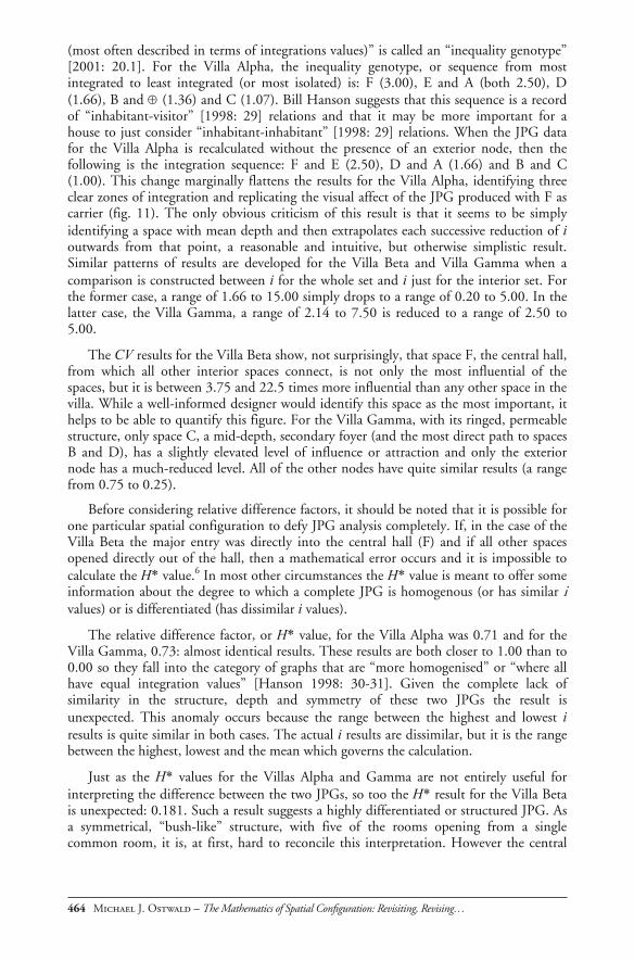
(most often described in terms of integrations values)” is called an “inequality genotype” [2001: 20.1]. For the Villa Alpha, the inequality genotype, or sequence from most integrated to least integrated (or most isolated) is: F (3.00), E and A (both 2.50), D (1.66), B and (1.36) and C (1.07). Bill Hanson suggests that this sequence is a record of “inhabitant-visitor” [1998: 29] relations and that it may be more important for a house to just consider “inhabitant-inhabitant” [1998: 29] relations. When the JPG data for the Villa Alpha is recalculated without the presence of an exterior node, then the following is the integration sequence: F and E (2.50), D and A (1.66) and B and C (1.00). This change marginally flattens the results for the Villa Alpha, identifying three clear zones of integration and replicating the visual affect of the JPG produced with F as carrier (fig. 11). The only obvious criticism of this result is that it seems to be simply identifying a space with mean depth and then extrapolates each successive reduction of i outwards from that point, a reasonable and intuitive, but otherwise simplistic result. Similar patterns of results are developed for the Villa Beta and Villa Gamma when a comparison is constructed between i for the whole set and i just for the interior set. For the former case, a range of 1.66 to 15.00 simply drops to a range of 0.20 to 5.00. In the latter case, the Villa Gamma, a range of 2.14 to 7.50 is reduced to a range of 2.50 to 5.00.

The CV results for the Villa Beta show, not surprisingly, that space F, the central hall, from which all other interior spaces connect, is not only the most influential of the spaces, but it is between 3.75 and 22.5 times more influential than any other space in the villa. While a well-informed designer would identify this space as the most important, it helps to be able to quantify this figure. For the Villa Gamma, with its ringed, permeable structure, only space C, a mid-depth, secondary foyer (and the most direct path to spaces B and D), has a slightly elevated level of influence or attraction and only the exterior node has a much-reduced level. All of the other nodes have quite similar results (a range from 0.75 to 0.25).

Before considering relative difference factors, it should be noted that it is possible for one particular spatial configuration to defy JPG analysis completely. If, in the case of the Villa Beta the major entry was directly into the central hall (F) and if all other spaces opened directly out of the hall, then a mathematical error occurs and it is impossible to calculate the H* value.6 In most other circumstances the H* value is meant to offer some information about the degree to which a complete JPG is homogenous (or has similar i values) or is differentiated (has dissimilar i values).

The relative difference factor, or H* value, for the Villa Alpha was 0.71 and for the Villa Gamma, 0.73: almost identical results. These results are both closer to 1.00 than to 0.00 so they fall into the category of graphs that are “more homogenised” or “where all have equal integration values” [Hanson 1998: 30-31]. Given the complete lack of similarity in the structure, depth and symmetry of these two JPGs the result is unexpected. This anomaly occurs because the range between the highest and lowest i results is quite similar in both cases. The actual i results are dissimilar, but it is the range between the highest, lowest and the mean which governs the calculation.

Just as the H* values for the Villas Alpha and Gamma are not entirely useful for interpreting the difference between the two JPGs, so too the H* result for the Villa Beta is unexpected: 0.181. Such a result suggests a highly differentiated or structured JPG. As a symmetrical, “bush-like” structure, with five of the rooms opening from a single common room, it is, at first, hard to reconcile this interpretation. However the central


controlling hall, room F, has a very high integration value, much higher than the remainder of the rooms, supporting one particular interpretation of the idea of differentiated or structured space.

Ultimately, the use of H* values for the analysis of three simple structures, which are already almost archetypes, is not terribly informative and a larger and more complex body of data is required to really test the interpretation of this part of the method.

Conclusion

It is difficult to support the criticism that the mathematics of the JPG method has rarely been consistently presented in its totality since it was first formulated but the task of reconstructing it remains complex, time consuming and especially involved for the general scholar. Perhaps because it was explained in so much detail in the early work of Steadman [1973: 1983], subsequent works have presented only isolated stages of the method. Similarly, perhaps because Hillier’s and Hanson’s major works were developed while the JPG method was still being formulated and tested, it was never given the full space it deserved. Finally, as time has passed, the major developments in JPG analysis have tended to be recorded in scattered journal and conference papers, making the task of finding, evaluating and combining works especially demanding. Once a consistent analytical method has been developed, then the problem becomes focussed on the more divisive issue of what it all means [Leach 1978: Osman and Suliman 1994: Dovey 2010].

However, despite concurring with some of the concerns raised about the mathematics and theory of the JPG, what is certain is that the larger the sample size, the more interesting the results become. For example, the studies of seventeen vernacular farmhouses in Normandy [Hillier et al. 1987], seven Pueblo “room-blocks” [Shapiro 1995] and eighteen post-war suburban houses in London [Hanson 1998] are all informative because the body of data being analysed is large enough to not only make comparisons between the various values (TD, i, CV etc.) but to develop hypothetical genotypes for such sets. A structural genotype is a socially authorised, ideal spatial configuration, for a particular programmatic type. It can be identified through the close analysis of multiple instances of the same type, in the same social or cultural setting. Dovey argues that the “great achievement of spatial syntax analysis has been … [to] reveal a social ideology embedded in structural genotypes” [1999: 24]. The genotype can really only be uncovered if there is a sufficiently large set of examples being studied and thus the JPG method is most useful when applied to sets of buildings in a consistent way.

Finally, there is a dimension of JPG research that has not yet been adequately developed. While the JPG has been used to compare social patterns in a range of historic and vernacular homes or villages and in some modern housing estates, there are few examples of the method being used to analyse the body of work of an individual architect [Major and Sarris 1999; Bafna 2001]. Hanson [1998] certainly analyses some isolated architect-designed houses; she also constructs a social comparison between architect-designed and non-architect-designed houses, but this isn’t the same thing. While Space Syntax and the JPG are commonly presented as being an approach to understanding social patterns embedded in a spatial configuration, they can also be used to obtain insights into the way designers think about space and into the social values they embody in their work. Thus, instead of developing a genotype for the comparative analysis of English cottages, or French farmhouses, one could be developed for Frank Lloyd Wright’s prairie houses, Le Corbusier’s villas or Glenn Murcutt’s rural homes. There is at least one good precedent for this: Sonit Bafna’s [2001] study of Miesian courtyard


houses, which, while largely concentrated on methodological issues, provides an important template for future analysis. Through the focussed analysis of an architect’s work it would be possible not only to interrogate their actual social and cultural values, and to compare them with their espoused views, but it may also be possible to trace the development of their design approaches over the course of their careers. It is this territory of design analysis, previously largely ignored by proponents of the JPG method, which is potentially most relevant for its revival.

Acknowledgments

I would like to acknowledge the detailed, insightful and supportive comments of Professor John Peponis. An ARC Fellowship (FT0991309) and an ARC Discovery Grant (DP1094154) supported the research undertaken in this paper. All of the images in the paper are by Romi McPherson for the author.

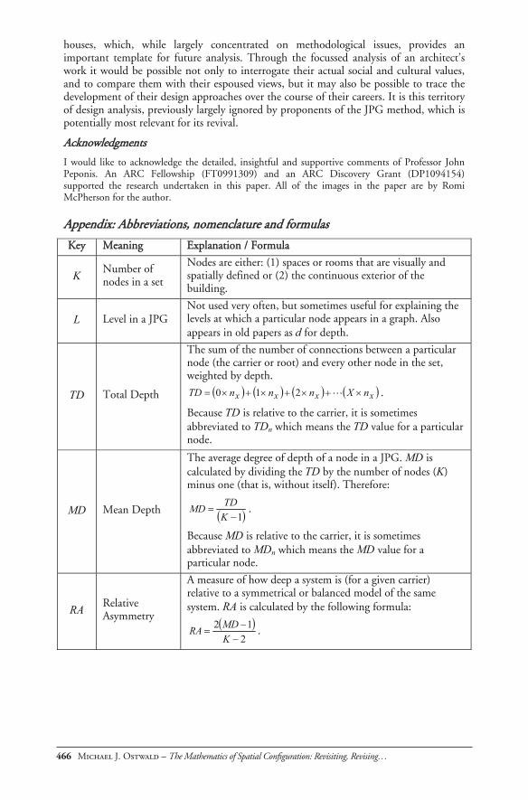
Appendix: Abbreviations, nomenclature and formulas

Key Meaning Explanation / Formula

K Number of nodes in a set

Nodes are either: (1) spaces or rooms that are visually and spatially defined or (2) the continuous exterior of the building.

L Level in a JPG Not used very often, but sometimes useful for explaining the levels at which a particular node appears in a graph. Also appears in old papers as d for depth.

TD Total Depth

The sum of the number of connections between a particular node (the carrier or root) and every other node in the set, weighted by depth.

xxxx nXnnnTD 210 .

Because TD is relative to the carrier, it is sometimes abbreviated to TDn which means the TD value for a particular node.

MD Mean Depth

The average degree of depth of a node in a JPG. MD is calculated by dividing the TD by the number of nodes (K) minus one (that is, without itself). Therefore:

1KTDMD .

Because MD is relative to the carrier, it is sometimes abbreviated to MDn which means the MD value for a particular node.

RA Relative Asymmetry

A measure of how deep a system is (for a given carrier) relative to a symmetrical or balanced model of the same system. RA is calculated by the following formula:

212

KMDRA .


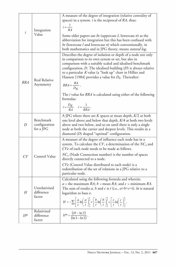
i Integration Value

A measure of the degree of integration (relative centrality of spaces) in a system. i is the reciprocal of RA, thus:

RAi 1

Some older papers use In (uppercase I, lowercase n) as the abbreviation for integration but this has been confused with ln (lowercase l and lowercase n) which conventionally, in both mathematics and in JPG theory, means natural log.

RRA Real Relative Asymmetry

Describes the degree of isolation or depth of a node not only in comparison to its own system or set, but also in comparison with a suitably scaled and idealised benchmark configuration, D. The idealised building (D) is always relative to a particular K value (a “look up” chart in Hillier and Hanson [1984] provides a value for DK. Thereafter:

KDRARRA .

The i value for RRA is calculated using either of the following formulas:

RADi K

RRAi 1 .

D Benchmark configuration for a JPG

A JPG where there are K spaces at mean depth, K/2 at both one level above and below that depth, K/4 at both two levels above and two below, and so on until there is only a single node at both the carrier and deepest levels. This results in a diamond (D) shaped “optimal” configuration.

CV Control Value

A measure of the degree of influence each node has in a system. To calculate the CV, a determination of the NCn and CVe of each node needs to be made as follows.

NCn (Node Connection number) is the number of spaces directly connected to a node.

CVe (Control Value distributed to each node) is a redistribution of the set of relations in a JPG relative to a particular node.

H Unrelativised difference factor

Calculated using the following formula and wherein: a = the maximum RA; b = mean RA; and c = minimum RA. The sum of results a, b and c is t (i.e., a+b+c=t). ln is natural logarithm to base e.

tc

tc

tb

tb

ta

taH lnlnln .

H* Relativised difference factor 2ln3ln

2ln* HH .


Notes 1. As part of the research undertaken for this paper a review of over fifty publications on the JPG

method, spanning from the early 1970s to the present, was undertaken. This review noted in the early papers a not unexpected lack of consistency in nomenclature, interpretation and mathematical basis. Conversely, many recent papers have a tendency to rely blindly on software, a process which completely hides the mathematics of the operation and which ignores the possibility that the software might be wrong. On those occasions when the formulas were published in papers and it was possible to check the veracity of the results a surprising number of mathematical errors were uncovered.

2. In statistical analysis such a process is usually undertaken using “Z-scores”. This works by standardising the complete set of results around two parameters: the mean is set at 0 and the spread of results is distributed in such a way as to attain a standard deviation of 1. This will produce a set of results arrayed around the 0 point with the negative results being below the original mean and the positive above it.

3. Hanson [1998: 28] offers one of the very few worked examples in the JPG field but it features a mis-transcribed figure for an MD result (the correct result of the MD calculation, 4.78, is mistyped as an MD value of 4.87 in the following RA calculation) meaning that her results are compromised.

4. Note that ln in the formula is natural logarithm to base e, not In, short for integration, a common error in papers using old nomenclature, or 1n, another mistake repeated in the JPG literature

5. For this paper all of the initial calculations were completed “by hand” to confirm the method and then mathematically scripted in a scientific calculator program for subsequent operations. At the completion of the worked examples, AGraph software (vers. 1.14) was used as a final check of results. While AGraph was an excellent tool for the majority of the process, it does not correctly calculate H and H* results using natural logarithms and does not handle irrational numbers correctly.

6. A methodological problem occurs when the total depth of a node equals the number of rooms, minus one. That is, MD = 1.00: a room which is connected to every other room. The problem occurs because the Relative Asymmetry calculation (step 4a) produces an irrational result for the special case of a room that connects to every other room. This is a problem because the following stage (step 5a) seeks the reciprocal of the irrational number, which leads to H and H* values being impossible to calculate for the chosen dwelling.

References ALEXANDER, Christopher. 1964. Notes on the synthesis of form. Cambridge, MA: Harvard

University Press. ———. 1966. A City is Not a Tree, Part I and Part II. Design 2206 (February 1966): 46-55. ALEXANDER, Christopher, Sara ISHIKAWA and Murray SILVERSTEIN. 1977. A Pattern Language:

towns, buildings, construction. New York: Oxford University Press. ASAMI, Yasushi, Ayse Sema KUBAT, Kensuke KITAGAWA and Shin-ichi IIDA. 2003. Introducing the

third dimension on Space Syntax: Application on the historical Istanbul. Proceedings: 4th International Space Syntax Symposium London: 48.1-48.18.

BAFNA, Sonit. 2001. Geometric Intuitions of Genotypes. Proceedings of the Third International Symposium on Space Syntax, 20.1-20.16.

———. 2003. Space Syntax: a Brief Introduction to its Logic and Analytical Techniques. Environment and Behavior 335, 1: 17-29.

BIRKERTS, Gunnar. 1994. Process and Expression in Architectural Form. Norman: University of Oklahoma Press.

CHING, Francis D. K. 2007. Architecture: Form, Space and Order. Hoboken, NJ: John Wiley and Sons.

DOVEY, Kim 2010. Becoming Places: Urbanism / Architecture / Identity / Power. London: Routledge.

———. 1999. Framing Places: Mediating Power in Built Form. London: Routledge.


FRAMPTON, Kenneth. 1995. Studies in Tectonic Culture: The Poetics of Construction in Nineteenth and Twentieth Century Architecture. Cambridge, MA: MIT Press.

GELERNTER, Mark. 1995. Sources of Architectural Form: A Critical History of Western Design Theory. New York: St. Martin’s Press.

HANSON, Julienne. 1998. Decoding Homes and Houses. Cambridge: Cambridge University Press. HAQ, S. 2003 Investigating the syntax line: configurational properties and cognitive correlates.

Environment and Planning B: Planning and Design 30: 841-863. HARARY, Frank. 1960. Some Historical and Intuitive Aspects of Graph Theory. SIAM Review 22, 2

(April 1960): 123-131. ———. 1969. Graph Theory. Reading, MA: Addison-Wesley. HILLIER, Bill. 1995. Space is the Machine, Cambridge: Cambridge University Press.. HILLIER, Bill and Alan PENN. 2004. Rejoinder to Carlo Ratti. Environment and Planning B_

Planning and Design 331, 4: 487–499. Hillier, Bill and Julienne HANSON. 1984. The Social Logic of Space. New York: Cambridge

University Press. Hillier, Bill and Kali TZORTZI. 2006. Space Syntax: The Language of Museum Space. Pp. 282-301

in A Companion to Museum Studies, Sharon Macdonald, ed. London: Blackwell. HILLIER, Bill, Julienne HANSON and H. GRAHAM. 1987. Ideas are in things: an application of the

space syntax method to discovering house genotypes. Environment and Planning B: Planning and Design 114: 363-385.

HOPKINS, Brian and Robin J. WILSON. 2004. The Truth about Königsberg. The College Mathematics Journal 335, 3 (May 2004): 198-207.

JENCKS, Charles and George BAIRD, eds. 1969. Meaning in Architecture. New York: G. Braziller. JIANG, Bin, Christophe CLARAMUNT and Björn KLARQVIST. 2000. Integration of space syntax into

GIS for modelling urban spaces. International Journal of Applied Earth Observation and Geoinformation 2, 3-4: 161-171.

KLARQVIST, Björn. 1993. A Space Syntax Glossary. Nordisk Arkitekturforskning 22: 11-12. KRÜGER, M. 1989. On Node and Axial Grid Maps: Distance measures and related topics, London:

University College, London. LEACH, Edmund. 1978. Does Space Syntax Really "Constitute the Social"? Pp. 385-401 in Social

Organisation and Settlement. Contributions from Anthropology, Archaeology and Geography, D. Green and M. Spriggs, eds. British Archaeology Reports 47. Oxford.

MAJOR, Mark David and Nicholas SARRIS. 1999. Cloak and Dagger Theory: Manifestations of the Mundane in the Space of Eight Peter Eisenman Houses. Space Syntax: Second International Symposium, Brasilia. 20.1-20.14.

MANUM, Bendik. 2009. AGRAPH: Complementary Software for Axial-Line Analysis. In Proceedings of the 7th International Space Syntax Symposium. Daniel Koch, Lars Marcus and Jesper Steen, eds. Stockholm: KTH, 2009. 070:1

MANUM, Bendik, Espen RUSTEN and Paul BENZE. 2005. AGRAPH, Software for Drawing and Calculating Space Syntax Graphs. Proceedings of the 5th International Space Syntax Symposium, vol. I, 97. Delft.

MARCH, Lionel, ed. 1976. The Architecture of Form. Cambridge: Cambridge University Press. MARCH, Lionel and Philip STEADMAN. 1971. The Geometry of Environment: An introduction to

spatial organization in design. London: RIBA Publications. MARKUS, Tom. 1987. Buildings as Classifying Devices. Environment and Planning B: Planning

and Design 114: 467-484. ———. 1988. Down to Earth. Building Design (July 15): 16-17. ———. 1993. Buildings and Power. London: Routledge. OSMAN, Khadiga M. and Mamoun SULIMAN. 1994. The Space Syntax Methodology: Fits and

Misfit. Architecture & Behaviour 10, 2: 189-204. PALLASMAA, Juhani. 2005. The eyes of the skin: architecture and the senses. Chichester: Wiley-

Academy. PEPONIS, John. 1985. The spatial culture of factories. Human Relations 338 (April 1985): 357-390.


PEPONIS, John, Jean WINEMAN, Mahbub RASHID, S. KIM, and Sonit BAFNA. 1997a. On the description of shape and spatial configuration inside buildings: convex partitions and their local properties. Environment and Planning B: Planning and Design 224: 761-781.

———. 1997b. On the generation of linear representations of spatial configuration. Space Syntax, First International Symposium, vol III, 4.1-41.18. London.

PEVSNER, Nikolaus. 1936. Pioneers of Modern Design. London: Faber and Faber. RATTI, Carlo. 2004. Space syntax: some inconsistencies. Environment and Planning B: Planning

and Design 331, 4: 501–511. ROWLAND, Ingrid D. and Thomas Noble HOWE, eds. 1999. Vitruvius: Ten Books on

Architecture. Cambridge: Cambridge University Press. SEPPÄNEN, Jouko and James M. MOORE. 1970. Facilities Planning with Graph Theory.

Management Science 117, 4 (December 1970): 242-253. SHANNON, C. E. 1949. The Mathematical Theory of Communication. Urbana, IL: University of

Illinois. SHAPIRO, Jason. S. 2005. A Space Syntax Analysis of Arroyo Hondo Pueblo, New Mexico. Santa

Fe: School of American Research Press. STEADMAN, Philip J. 1973. Graph-theoretic representation of architectural arrangement.

Architectural Research and Teaching 22: 161-172. ———. 1983. Architectural Morphology. London: Pion. STEVENS, Garry. 1990. The Reasoning Architect: Mathematics and Science in Design. New York:

McGraw Hill. STINY, George. 1975. Pictorial and Formal Aspects of Shape and Shape Grammar. Basel:

Birkhäuser. TAAFFE E. J. and H. L. GAUTHIER. 1973. Geography of Transportation. New Jersey: Prentice Hall. TEKLENBERG, J. A. F. TIMMERMANS, H. J. P. WAGENBERG, A. F. 1992. Space Syntax:

Standardized integration measures and some simulations. Environment and Planning B: Planning and Design 20: 347-357.

THALER, Ulrich. 2005. Narrative and Syntax, new perspectives on the Late Bronze Age palace of Pylos, Greece. Proceedings of the 5th International Space Syntax Symposium, vol. II, 327. Delft.

TURNER, A., M. Doxa, D. O’Sullivan, A. Penn. 2001. From isovists to visibility graphs: a methodology for the analysis of architectural space. Environment and Planning B: Planning and Design 28: 103-121.

XINQI, Zheng, Zhao LU, Fu MEICHEN and Wang SHUQING. 2008. Extension and Application of Space Syntax: A Case Study of Urban Traffic Network Optimizing in Beijing. IEEE Workshop on Power Electronics and Intelligent Transportation System: 291-295.

ZAKO, Reem. 2006. The power of the veil: Gender inequality in the domestic setting of traditional courtyard houses. Pp. 65-75 in Courtyard Housing: Past, Present and Future, Brian Edwards, Magdo Sibley, Mohamad Hakmi and Peter Land, eds. New York: Taylor and Francis.

About the author Professor Michael J. Ostwald is Dean of Architecture at the University of Newcastle (Australia), Visiting Professor at RMIT University (Melbourne) and a Professorial Fellow at Victoria University Wellington (New Zealand). He has a Ph.D. in architectural history and theory and a higher doctorate (D. Sc) in the mathematics of design. He has lectured in Asia, Europe and North America and has written and published extensively on the relationship between architecture, philosophy and geometry. He has a particular interest in fractal, topographic and computational geometry and has been awarded many international research grants in this field. Michael Ostwald is a member of the editorial boards of the Nexus Network Journal and Architectural Theory Review and he is co-editor of the journal Architectural Design Research. He has authored more than 250 scholarly publications, including 20 books. His recent books include The Architecture of the New Baroque (2006), Residue: Architecture as a Condition of Loss (2007), Homo Faber 1: Modelling Design (2008), Homo Faber 2: Modelling Ideas (2008) and Understanding Architectural Education in Australasia (2009). He is also co-editor of Museum, Gallery and Cultural Architecture in Australia, New Zealand and the Pacific Region (2007).

Date post:	20-Mar-2020
Category:	Documents
Upload:	others
View:	20 times
Download:	0 times

Michael J. Ostwald Research - Springer · 446 Michael J. Ostwald – The Mathematics of Spatial...

Documents