Microbial Risk Assessment Guideline: Pathogenic ...MICROBIAL RISK ASSESSMENT GUIDELINE PATHOGENIC...

MICROBIAL

RISK ASSESSMENT GUIDELINE

PATHOGENIC MICROORGANISMS

WITH FOCUS ON FOOD AND WATER

Prepared by the Interagency Microbiological

Risk Assessment Guideline

Workgroup

July 2012

Publication Numbers:

USDA/FSIS/2012-001

EPA/100/J12/001

October 2010

Microbial Risk Assessment Guideline Page ii

DISCLAIMER

This guideline document represents the current thinking of the workgroup on the topics

addressed. It is not a regulation and does not confer any rights for or on any person and does

not operate to bind USDA, EPA, any other federal agency, or the public. Further, this

guideline is not intended to replace existing guidelines that are in use by agencies. The

decision to apply methods and approaches in this guideline, either totally or in part, is left

to the discretion of the individual department or agency.

Mention of trade names or commercial products does not constitute endorsement or

recommendation for use.

Citation

U.S. Department of Agriculture/Food Safety and Inspection Service (USDA/FSIS) and U.S.

Environmental Protection Agency (EPA) (2012). Microbial Risk Assessment Guideline:

Pathogenic Organisms with Focus on Food and Water. FSIS Publication No.

USDA/FSIS/2012-001; EPA Publication No. EPA/100/J12/001.

Microbial Risk Assessment Guideline Page iii

TABLE OF CONTENTS

Disclaimer .......................................................................................................................... ii

Interagency Workgroup Members ................................................................................ vii

Preface ............................................................................................................................. viii

Abbreviations ................................................................................................................... ix

Executive Summary…………………………………………………………………….xii

1. Introduction .................................................................................................................. 1 1.1 Who is this Guideline Written For? ................................................................. 1

1.2 What are the Benefits of this Guideline? ......................................................... 2

1.3 What are Some Fundamental Differences between Microbes and

Chemicals? .......................................................................................................... 3 1.4 What are the Components of a MRA that I Should Consider? ..................... 6

1.5 How is this MRA Guidance Related to Other MRA

Frameworks/Guidelines that are Currently Available? ................................. 8 1.6 What MRA Principles MRA Should I be Aware Of? .................................... 9

1.7 How can the MRA be Used? ........................................................................... 11 1.8 What Are Examples of Types of MRA? ........................................................ 12

1.9 What Types of Decisions within Risk Assessment are Science Policy?....... 13 1.10 Why are Uncertainty and Variability in MRA Important? ......................... 15 1.11 Summary ........................................................................................................... 16

2. Planning and Scoping ................................................................................................ 17 2.1 What is Planning and Scoping? ...................................................................... 17

2.1.1 What is Problem Formulation? ............................................................ 18

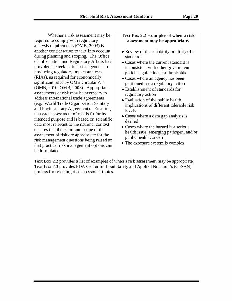
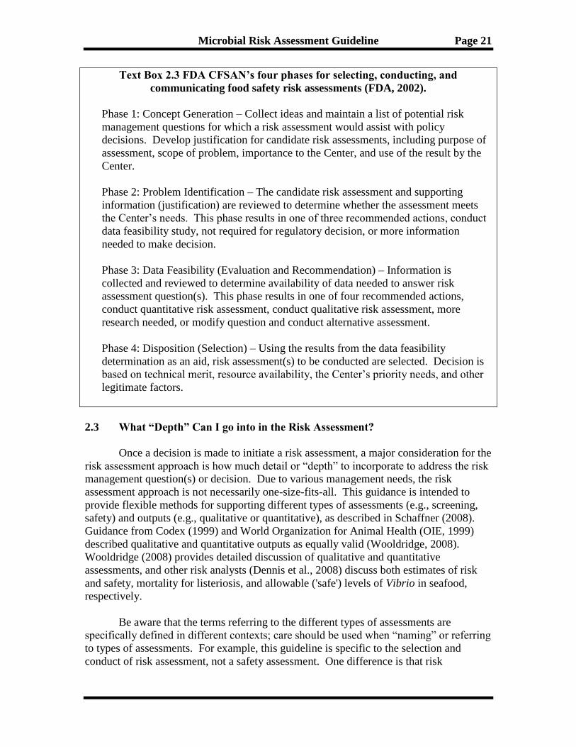
2.2 What do I Consider When Deciding to Initiate a MRA? ............................. 19 2.3 What “Depth” Can I go into in the Risk Assessment? ................................. 21 2.4 What Elements are Discussed During Planning and Scoping? ................... 23

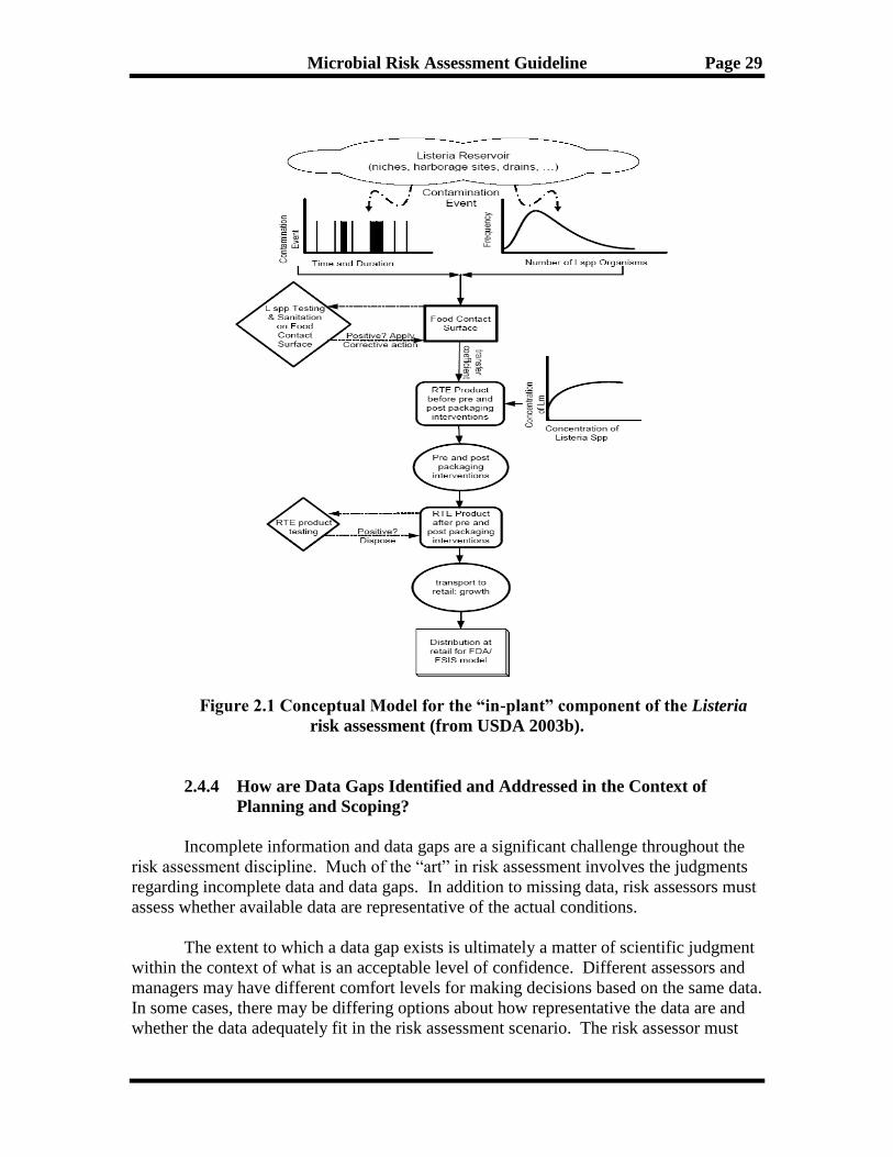
2.4.1 What are Risk Management Questions and What is the Charge? ... 27 2.4.2 What is a Risk Profile? ......................................................................... 27 2.4.3 What is a Conceptual Model? .............................................................. 28

2.4.4 How are Data Gaps Identified and Addressed in the Context of

Planning and Scoping? .......................................................................... 29

2.4.5 What is an Analysis Plan? .................................................................... 32

2.4.6 How do I Consider Information Quality Including Data Quality? .. 32

2.4.7 What is Value-of-Information Analysis? ............................................ 35 2.4.8 What is a Communications Plan? ........................................................ 35

2.5 Who Can be Involved with Planning and Scoping? ..................................... 36 2.6 Summary ........................................................................................................... 37

3. Hazard Identification and Hazard Characterization ............................................. 38 3.1 What are Hazard Identification and Hazard Characterization? ................ 38

Microbial Risk Assessment Guideline Page iv

3.2 How do I Define the Hazard? ......................................................................... 39

3.3 What Hazard Characteristics Can I Consider? ............................................ 40 3.4 How do Microbial Hazards Cause Adverse Outcomes? .............................. 41

3.4.1 What does Virulence and/or Pathogenicity Mean in the Context of

Causing an Adverse Outcome? ............................................................ 42

3.5 What are the Mechanisms that May Lead to the Development of New

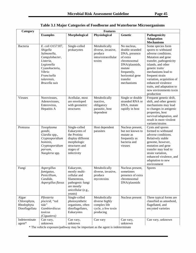
Pathogens or Pathogens with New Traits? .................................................... 43 3.6 What are the Major Categories of Microorganisms? ................................... 44

3.7 What Methodological Approaches are Used to Identify and Quantify

Microorganisms?.............................................................................................. 46 3.8 Are there Concerns Regarding Microbial Detection Methods? .................. 47 3.9 What Host Factors Can I Take into Consideration? .................................... 51

3.10 How does Life Stage Affect Sensitivity to Infection and Disease

Manifestation? .................................................................................................. 53 3.11 What Environmental Factors Can I Take into Consideration? .................. 54

3.12 Summary ........................................................................................................... 55

4. Dose-Response Assessment ....................................................................................... 56 4.1 What is Dose-Response Modeling and What are Some General

Considerations for Dose-Response Modeling? .............................................. 56

4.1.1 How do I Choose Between Modeling a Discrete Dose Versus an

Average Dose? ........................................................................................ 57

4.1.2 What is the Difference Between a Threshold and a Non-Threshold

Model? .................................................................................................... 58 4.1.3 What is the One-Hit Model and When is it the Preferred Model? ... 58

4.1.4 What Important Factors Can I Consider in Dose-Response

Assessment? ........................................................................................... 60 4.1.5 How Can I Model the Spread of Disease in the Population?............. 67 4.1.6 What Can I Address for Each Model to Improve Transparency? ... 69

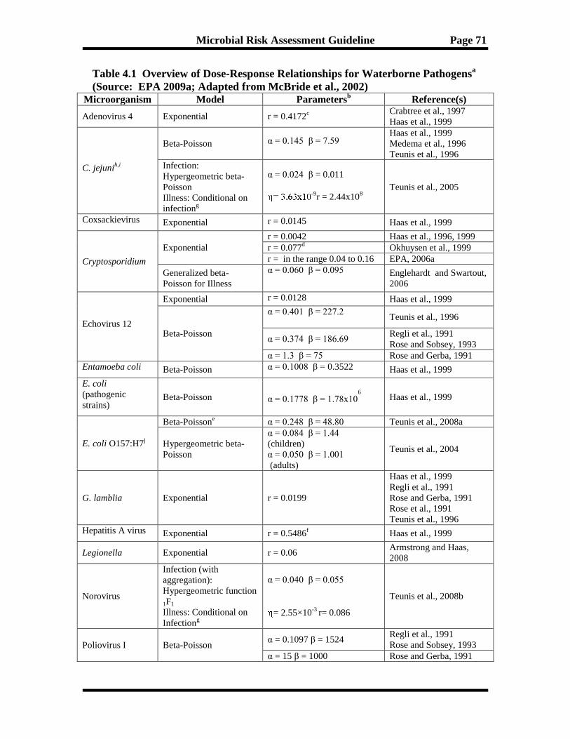
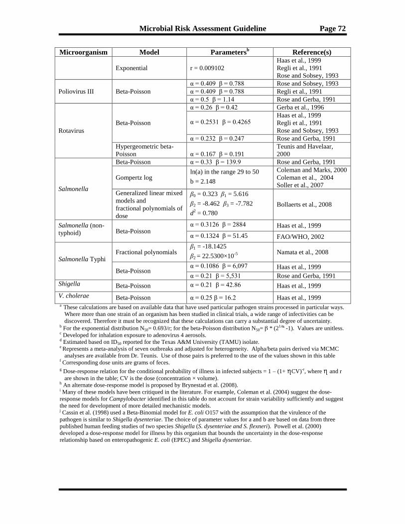
4.2 What is Current Practice in Quantitative Dose-Response Modeling for

Microbial Illness? ............................................................................................. 70

4.2.1 What Models Can I Use for Microbial Dose-Response Assessment? 70 4.2.2 What is the Output of a Dose-Response Assessment?........................ 76

4.2.3 How do I Fit Models to Existing Dose-Response Data? ..................... 77 4.2.4 How Can I Evaluate Uncertainty in Dose-Response? ........................ 79 4.2.5 What is Variability in Dose-Response? ............................................... 80

4.2.6 How Can I Account for Life Stages and Different Populations in

Dose-Response Models? ........................................................................ 81

4.2.7 Can I Use Uncertainty, Modifying, or Adjustment Factors in a

Microbial Dose-Response Assessment? ............................................... 81

4.2.8 Are Other Modeling Methods Being Developed? ............................... 82 4.3 Summary ........................................................................................................... 83

5. Exposure Assessment ................................................................................................. 84 5.1 What are General Concepts in Exposure Assessment? ................................ 84

5.1.1 What is an Exposure Assessment? ....................................................... 84

Microbial Risk Assessment Guideline Page v

5.1.2 What are Sources, Pathways, and Routes of Exposure? ................... 85

5.1.3 How are Fate and Transport Considered in Exposure Assessment? 88 5.1.4 What Environmental Factors Can I Take into Consideration?........ 89 5.1.5 What is an Exposure Scenario? ........................................................... 90

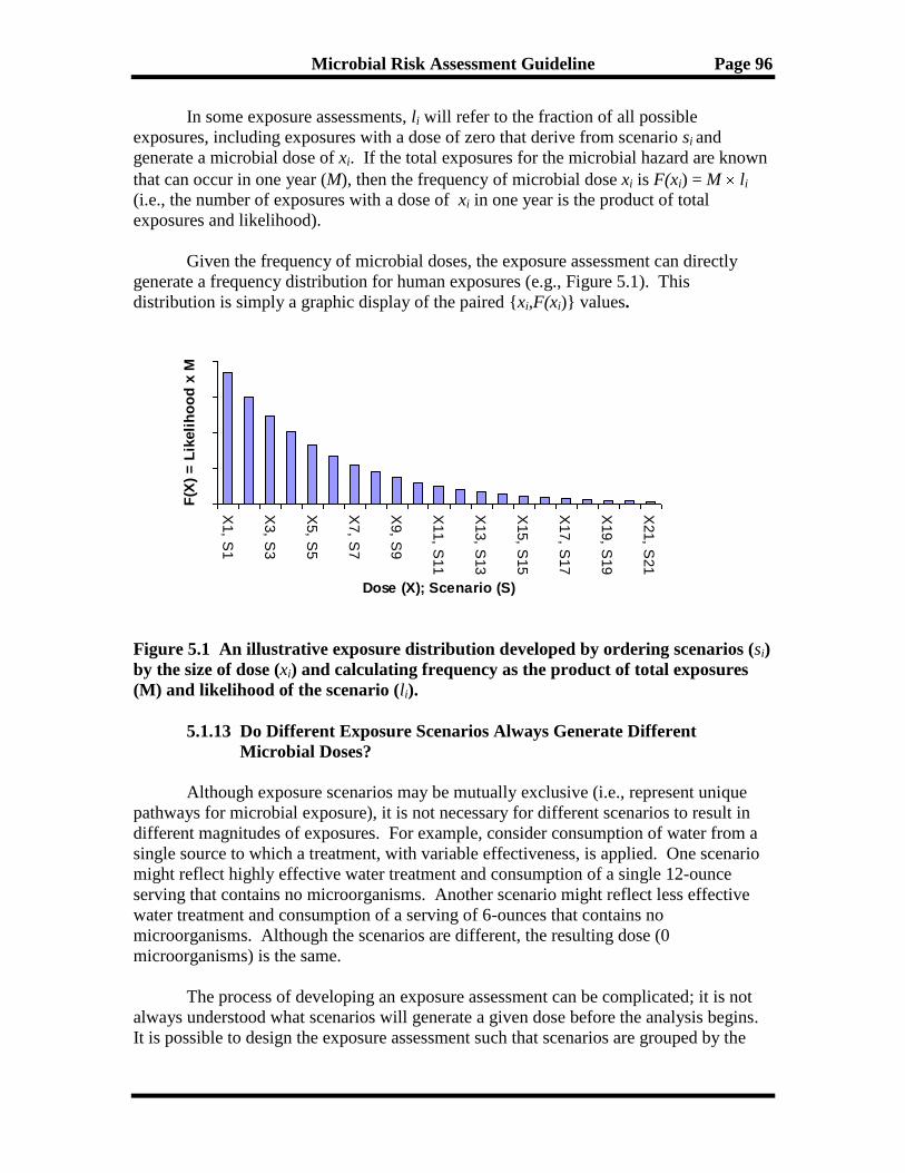
5.1.6 What are Qualitative and Quantitative Exposure Assessments? ..... 90 5.1.7 What is Variability in Exposure Assessment? .................................... 91 5.1.8 What is Uncertainty in Exposure Assessment? .................................. 91 5.1.9 What is a Deterministic Exposure Assessment? ................................. 92 5.1.10 What is a Stochastic Exposure Assessment? ....................................... 92

5.1.11 What is Monte Carlo Analysis? ........................................................... 93

5.1.12 How does Exposure Assessment Fit with the Other Components of

Risk Assessment? ................................................................................... 94

5.1.13 Do Different Exposure Scenarios Always Generate Different

Microbial Doses? ................................................................................... 96 5.2 How do I Develop an Exposure Assessment? ................................................ 98

5.2.1 What is the Purpose of the Exposure Assessment? ............................ 98 5.2.2 Which Scenarios Can I Consider? ....................................................... 99

5.2.3 What are the Exposed Populations I Could Consider? ................... 104 5.2.4 What Approaches to Exposure Modeling Can I Use? ..................... 105 5.2.5 How is Scenario Analysis Used in Exposure Assessment? .............. 111

5.2.6 What is the Role of Predictive Microbiology in Exposure

Assessment? ......................................................................................... 116

5.2.7 How Can I Address Secondary Transmission of Disease in the

Population? .......................................................................................... 118 5.2.8 What Data Can I Use in an Exposure Assessment? ......................... 120

5.2.9 How do I Use Data in an Exposure Assessment? ............................. 122

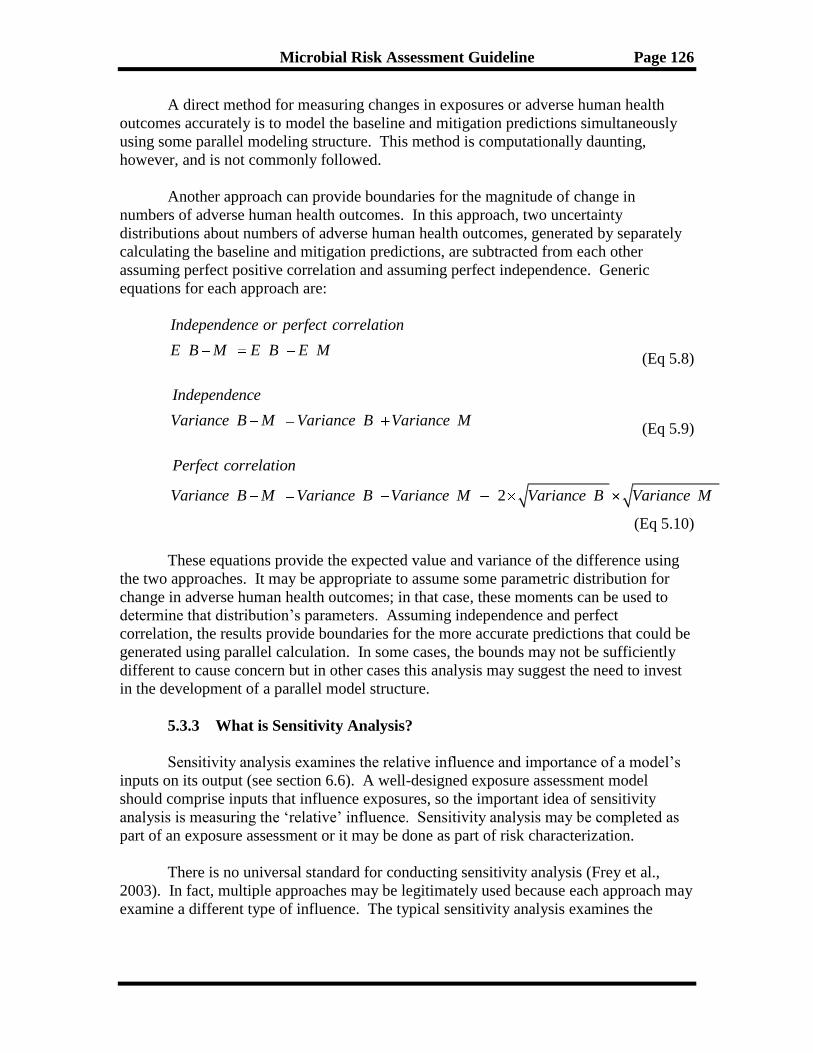
5.3 How do I Analyze a Model’s Results? .......................................................... 123 5.3.1 How do I Report Exposure in an Exposure Assessment? ................ 124 5.3.2 How do I Determine a Change in Exposure and Subsequent Risk?125

5.3.3 What is Sensitivity Analysis? .............................................................. 126 5.3.4 What is an Uncertainty Analysis? ...................................................... 127

5.4 What Can I Put Into an Exposure Assessment Report? ............................ 129 5.5 What are Possible Future Developments in Exposure Assessment? ......... 130

5.6 Summary ......................................................................................................... 131

6. Risk Characterization .............................................................................................. 133 6.1 What is Risk Characterization? ................................................................... 133 6.2 What are the Elements in a Risk Characterization? .................................. 134

6.3 How Do I Prepare a Risk Characterization? .............................................. 138

6.4 Are All Risk Characterizations Quantitative and What Do I Do When

Quantitative Data are Unavailable for Some Elements of the Risk

Characterization? .......................................................................................... 140

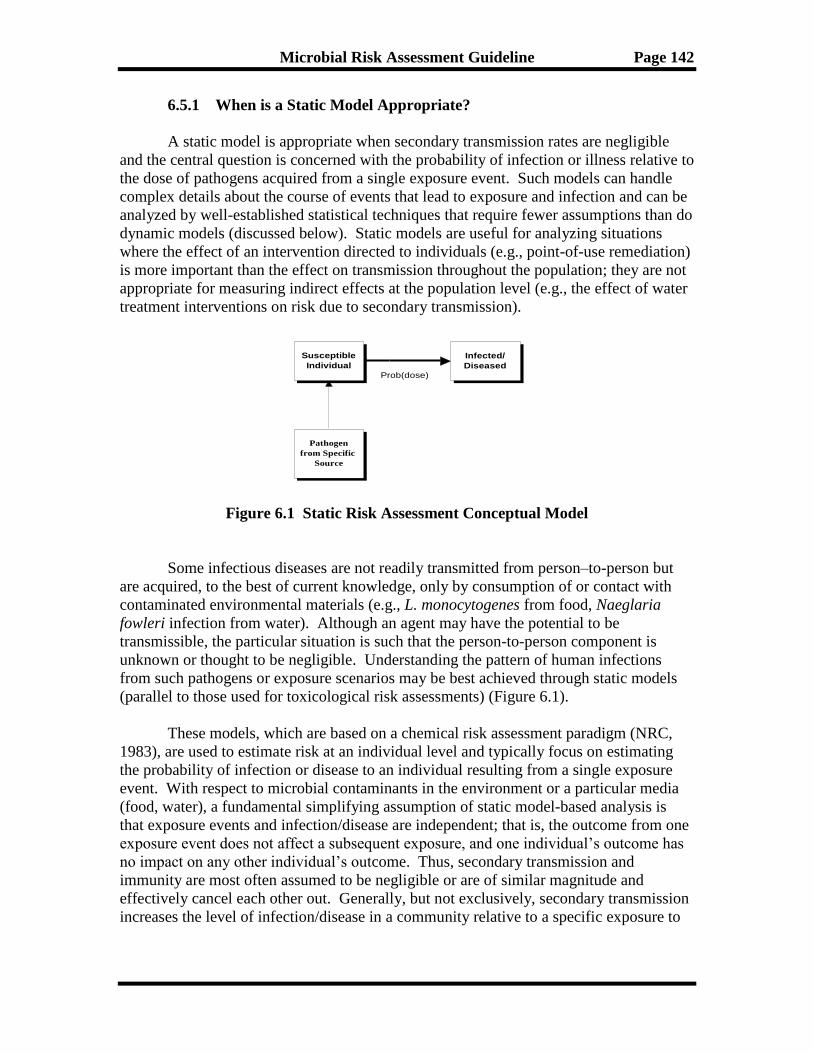
6.5 Are There Different Forms of Risk Characterization? When Do I Apply

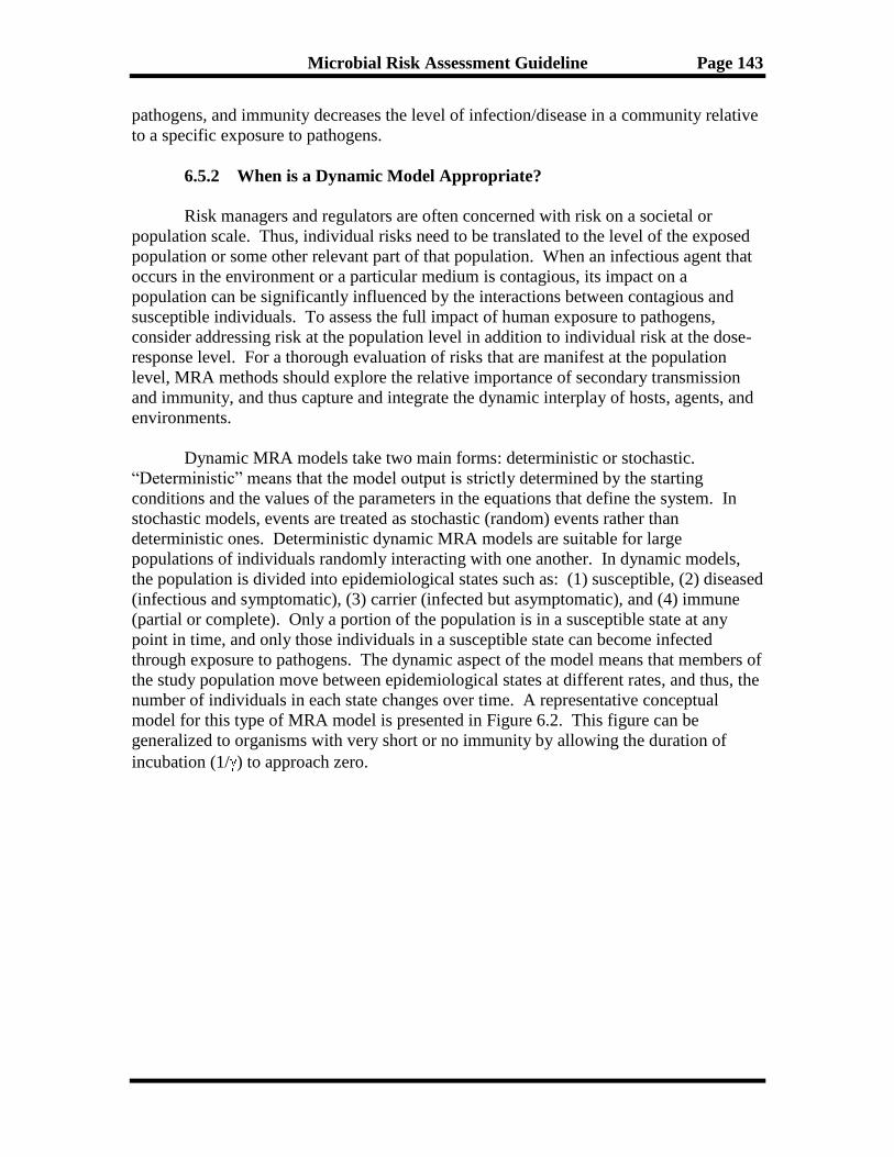
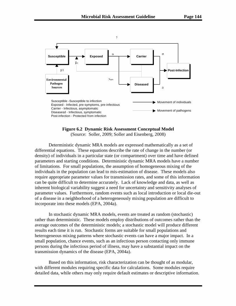
Them?.............................................................................................................. 140 6.5.1 When is a Static Model Appropriate? ................................................. 142 6.5.2 When is a Dynamic Model Appropriate? ........................................... 143

Microbial Risk Assessment Guideline Page vi

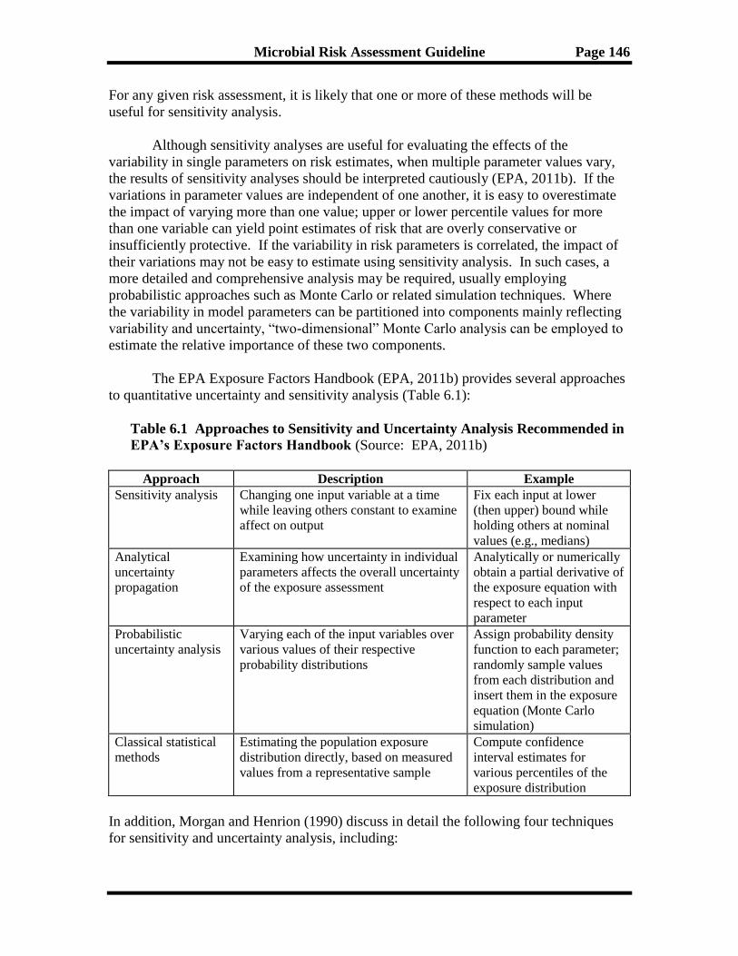
6.6 How are Sensitivity and Uncertainty Analyses Related to Risk

Characterization? .......................................................................................... 145 6.7 How are Quality of Life Measures Important in MRA? ............................ 147 6.8 How Can a Risk Assessment be Validated? ................................................ 148

6.9 Summary ......................................................................................................... 150

7. Risk Management .................................................................................................... 151 7.1 What is Risk Management? .......................................................................... 151 7.2 When and How Can Risk Managers be Involved in Risk Assessments? .. 153

7.3 How are Risk Management Options a Useful Component to Include in a

Risk Assessment? ........................................................................................... 155

7.4 What are Some Other Inputs into Risk Management Decisions About

Controlling or Accepting Risks?................................................................... 155

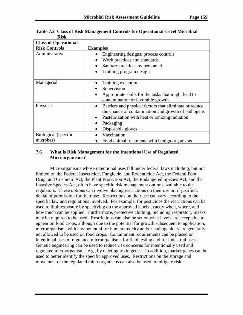
7.5 What are Some Operational Risk Management Tools and Approaches? 158

7.6 What is Risk Management for the Intentional use of Regulated

Microorganisms?............................................................................................ 159 7.7 Summary ......................................................................................................... 160

8. Risk Communication ............................................................................................... 161 8.1 What is Risk Communication? ..................................................................... 161

8.2 What are the Benefits of Risk Communication? ......................................... 161 8.3 Who are the Stakeholders of MRAs? ........................................................... 162

8.4 With Whom Can I Communicate? ............................................................... 163 8.5 When Can the Process of Risk Communication Begin? ............................ 164 8.6 Can I Communicate in Writing, Orally, or Both? ...................................... 164

8.7 Who Decides What to Communicate? ......................................................... 165

8.8 What Information Can be Communicated? ................................................ 165 8.9 How is the Communication Process a Continuous Dialog? ....................... 166 8.10 How In-Depth Can I Communicate? ........................................................... 166

8.11 What Can I Do if the Message is not “Getting Through?” ........................ 167 8.12 How Can I Communicate Risk Successfully? ............................................. 167

8.13 How Can I Handle Media and Congressional Office Requests? ............... 168 8.14 When Can Risk Communication End? ........................................................ 169

8.15 Summary ......................................................................................................... 170

9. Glossary .................................................................................................................... 171

10. References ............................................................................................................... 180

Appendix A Example Assumptions ............................................................................. A-1

Appendix B Hazard Identification Questions ............................................................ B-1

Microbial Risk Assessment Guideline Page vii

INTERAGENCY WORKGROUP MEMBERS

Kerry Dearfield, Co-Chair USDA/FSIS

Nicholas Ashbolt, Co-Chair EPA/ORD

Steve Schaub, Co-Chair (retired) EPA/OW

Michael Broder, Science Coordinator EPA/OSA

Irwin Baumel EPA/ORD

Uday Dessai USDA/FSIS

Eric Ebel USDA/FSIS

Brendlyn Faison EPA/OW

Joel Gagliardi EPA/OPP

Frank Hearl CDC/NIOSH

Abdel Kadry EPA/ORD

Janell Kause USDA/FSIS

Barbara Klieforth EPA/OSA

Ken Martinez CDC/NIOSH

Robert McDowell USDA/APHIS

Stephen Morse CDC/NCEZID

Tonya Nichols EPA/ORD

Mark Ott NASA

Duane Pierson NASA

Carl Schroeder USDA/FSIS

Mark Segal EPA/OPPT

Sean Shadomy CDC/NCEZID

Jeff Swartout EPA/ORD

Sarah Taft EPA/ORD

Brandolyn Thran DoD/AIPH

Elizabeth (Betsy) Weirich CDC/NCEZID

Other contributors (not currently on workgroup): Diane Henshel (EPA/OSA); Julie

Fitzpatrick (EPA/OSA); Bonnie Gaborek (USACHPPM); Myra Gardner (USDA/FSIS);

Alecia Naugle (USDA/FSIS); Geoff Patton (EPA/ORD); Gary Bangs (EPA/RAF);

Deborah McKean (EPA/ORD); Gregory Stewart (State); Parmesh Saini (USDA/FSIS);

Gregg Claycamp (FDA/CVM); Moshe Dreyfuss (USDA/FSIS); and William Schneider

(EPA/OPP)

Contractor support: Audrey Ichida (ICF International), Jeff Soller (Soller

Environmental), Sorina Eftim (ICF International), and Heather Simpson (ICF

International)

Microbial Risk Assessment Guideline Page viii

PREFACE

This Microbial Risk Assessment (MRA) guideline is written by microbial risk

assessors at the U.S. Department of Agriculture’s Food Safety and Inspection Service

(FSIS) and the U.S. Environmental Protection Agency (EPA). It serves as a resource for

these agencies, their agents, contractors, and stakeholders. Other Federal agencies

expressed interest in the development of this guideline and provided experts to participate

in this interagency effort (see list of participants). The working group followed the

Office of Management and Budget’s (OMB’s) Good Guidance Practices while

developing this guideline (OMB, 2007a).

In recognition of the needs and mandates of the participating agencies and the

various statutory authorities that may apply to MRA, this guideline emphasizes the need

for a flexible framework for conducting microbial risk assessment. It provides general,

broad fundamental risk assessment principles specifically for microbial risks, but as a

guideline it is not prescriptive nor does it supplant the internal practices or policies of any

Federal agency. Users have the flexibility to adapt pertinent sections to relevant statutory

authorities and purposes if needed. The intended audience is individuals with some

knowledge of microbiology and basic understanding of risk assessment principles but

some basics may be presented at the introduction to a topic. This guideline can be

periodically updated, particularly as more information becomes available.

The severity and duration of illness caused by exposure to pathogens vary

considerably. Many human pathogens found in food, water, and the environment cause

acute diseases that have short incubation periods, symptoms typically lasting several days

to a week, and usually non-lethal, common gastrointestinal effects but with complete

recovery from the illness. However, some pathogens associated with the gastrointestinal

tract may cause more serious diseases or sequelae, such as reactive arthritis, cancer,

Guillain-Barré syndrome, and juvenile-onset diabetes that may have long-term

implications. Further, there are indigenous water-based pathogens, such as Legionella

spp. and Mycobacterium spp., that can grow in biofilms and their inhalation via aerosols

may cause pneumonia. Some disease manifestations can be fatal. Applying risk

assessment approaches associated with MRA procedures discussed in this guideline help

risk assessors characterize the common exposure sources, causative agents, associated

symptoms, contributing immunity factors, and other common threads contributing to

chronic illness. This guideline is for human health MRAs, and does not include MRAs

conducted for ecological protection (e.g., wildlife, habitats).

This guideline does not specifically address scenarios related to biological warfare

agents, airborne microbial hazards, or agriculturally or industrially important

microorganisms, oligonucleotides, prions, preformed microbial toxins, and other

submicrobial entities. These agents have many unknowns associated with their sources,

modes of “infection” and disease, transmissibility, and survivability. Nonetheless,

information in this guideline may provide information to risk assessors addressing these

issues.

Microbial Risk Assessment Guideline Page ix

ABBREVIATIONS

ACSSuT Ampicillin, chloramphenicol, streptomycin, sulfonamides, and tetracycline

AFLP Amplified fragment length polymorphism

AIPH Army Institute of Public Health (formerly U.S. Army Center for Health

Promotion and Preventive Medicine [USA CHPPM])

ALOP Appropriate level of protection

AOAC Association of Analytical Communities

APHIS Animal and Plant Health Inspection Service (U.S. Department of

Agriculture)

ASM American Society for Microbiology

Bcc Burkholderia cepacia complex

BSE Bovine Spongiform Encephalopathy

°C degrees Celsius

CART Classification and regression tree

CARVER Criticality, Accessibility, Recuperability, Vulnerability, Effect, and

Recognizability

CDC Centers for Disease Control and Prevention

CEA cost-effectiveness analyses

CFSAN Center for Food Safety and Applied Nutrition

CFR Code of Federal Regulations

cfu colony forming unit

CWA Clean Water Act

DALYs Disability-adjusted life years

DHS Department of Homeland Security

DNA Deoxyribonucleic Acid

DOD Department of Defense

DT104 Definitive type 104 (p48)

ECSSC European Commission Scientific Steering Committee

EPA Environmental Protection Agency

°F degrees Fahrenheit

FAO Food and Agriculture Organization

FDA Food and Drug Administration

FIRRM Foodborne Illness Risk Ranking Model

FSIS Food Safety and Inspection Service

GI gastrointestinal

GRAS generally recognized as safe

gyrB DNA gyrase, subunit B

HACCP Hazard Analysis Critical Control Point

HC Hazard Characterization

HI Hazard Identification

HIV Human immunodeficiency virus

HYEs Healthy-years equivalents

ID50 Median Infectious dose

ILSI International Life Science Institute

LD50 Median lethal dose

Microbial Risk Assessment Guideline Page x

LT2ESWTR Long Term 2 Enhanced Surface Water Treatment Rule

MAC Mycobacterium avium-Complex

MCMC Markov Chain Monte Carlo Simulation

MILYs Morbidity Inclusive Life Years

MLGT Multilocus genotype sequencing

MLST Multilocus sequence typing

MRA microbial risk assessment

MRM microbial risk management

NASA National Aeronautics and Space Administration

NCEZID National Center for Emerging and Zoonotic Infectious Diseases

NCRP National Committee on Radiation Programs

NHANES National Health and Nutrition Examination Survey

NIOSH National Institute for Occupational Safety and Health (Centers for Disease

Control)

NOAEL No observable adverse effect level

NRC National Research Council

OECD Organization for Economic Cooperation and Development

OMB Office of Management and Budget

OPP Office of Pesticide Programs (US Environmental Protection Agency)

OPPT Office of Pollution Prevention and Toxics (US Environmental Protection

Agency)

ORD Office of Research and Development (US Environmental Protection

Agency)

OSA Office of the Science Advisor (US Environmental Protection Agency)

OW Office of Water (US Environmental Protection Agency)

P/CC Presidential/Congressional Commission

PCR Polymerase chain reaction

PCR-RFLP Polymerase chain reaction-restriction fragment length polymorphism

PFGE Pulsed field gel electrophoresis

pfu plaque forming units

QALYs Quality-adjusted life years

RAF Risk Assessment Forum (US Environmental Protection Agency)

RAPD Random amplification of polymorphic DNA

rDNA Ribosomal deoxyribonucleic acid

REP-PCR Repetitive element polymerase chain reaction

R&D Research and development

SARS Severe Acute Respiratory Syndrome

SDWA Safe Drinking Water Act

SNP Single nucleotide polymorphism

TAMU Texas A&M University

TB Tuberculosis

TCCR Transparency, Clarity, Consistency, and Reasonableness

U.S. United States

USDA U.S. Department of Agriculture

VBNC Viable-but-not-culturable

vCJD variant Creutzfeldt-Jacob Disease

Microbial Risk Assessment Guideline Page xi

VOI Value of information

WHO World Health Organization

Microbial Risk Assessment Guideline Page xii

EXECUTIVE SUMMARY

Modern societies have learned to reduce the impact of disease-causing

microorganisms (pathogens) by adopting various sanitary control measures, such as farm-

to-fork processes in food production and treatment plants for drinking water and

wastewater. Nonetheless, our aging and more vulnerable population groups combined

with the emergence of drug resistant pathogens and enhanced global spread of human

pathogens provides a breeding ground for novel and reemerging diseases. This microbial

risk assessment guidance document is written for risk assessors from participating federal

agencies to improve the quality and consistency of microbial risk assessments. The

guidance takes on a question/answer format for these practitioners to make it more

approachable by a wide audience.

While some federal agencies have an established record of conducting and

advancing chemical risk assessments (e.g., National Research Council reports, 2007,

2009), microbial risk assessment has not received as much attention or support. There

are several possible reasons for this but a significant one may be due to the challenges

posed by microbial risk assessments that are not considered in classical chemical risk

assessments. These challenges include the immune status of the host organism, person-

to-person transmission, and re-growth of pathogens both in the environment and in the

host. Further, no guideline has been previously developed by U.S. agencies addressing

the full process of microbial risk assessment. As a consequence, various approaches have

been used nationally, some based on the International Life Sciences Institute framework

for microbial risk assessment (ILSI, 1996, 2000).

The Microbial Risk Assessment Guideline: Pathogenic Microorganisms with

Focus on Food and Water addresses the entire risk assessment process from an

introduction to terminology and roles of the participants to planning the risk assessment,

identifying and characterizing the hazard, assessing how the size of an outbreak may be

affected by the dose (exposure assessment) or how the severity of the disease may be

affected by the pathogen and its response within the human host (dose-response

assessment). The document describes the importance of addressing the routes of

exposure, transport media, uncertainties, and assumptions for exposure and the other

components of the risk assessment paradigm when characterizing risk, and also provides

information about microbial risk management and risk communication. The goal of this

document is to produce a more harmonized treatment of microbial risk assessment across

participating federal agencies.

The Introduction (Chapter 1) lays out the purpose of the guideline, describing

some of the relevant history of the guideline and noting recommendations to develop a

microbial risk assessment guidance document based on the modified chemical risk

assessment paradigm. Next, Planning and Scoping (Chapter 2) describes the importance

of clearly identifying the purpose of the risk assessment at the outset. From the

articulated purpose, one determines the resources needed, including expertise, assesses

the current state of knowledge about the issue, and decides how to proceed with a clearly

defined vision of what the decision maker will need, ensuring that team members

understand the goals of the assessment and that they agree on the approach. The level of

Microbial Risk Assessment Guideline Page xiii

rigor applied during the planning and scoping phase of the risk assessment often has a

significant bearing on the quality and utility of the final product.

In order to properly conduct the risk assessment, the causative agent(s) must be

characterized (Chapter 3, Hazard Identification and Hazard Characterization). In the case

of an outbreak of a disease, the team typically works backwards evaluating possible

exposure pathways to the identified source of the pathogen(s). However, in many cases

the assessors start with known agent(s) and anticipated source-to-receptor scenario(s) in

an attempt to predict outcomes and to provide advice for risk management. In both cases,

a qualitative characterization of the hazard(s) and likely consequences of exposures are

identified with respect to potential human impact, including consideration of multiple life

stages.

Environmental stressors, biological or otherwise, normally exhibit an increasingly

pronounced effect with higher exposures, either in severity of the effect or fraction of the

population affected. As the host is exposed to more pathogens, the potential for disease

and/or the nature of the effect becomes more evident. This biological gradient is referred

to as the dose-response relationship (Chapter 4), which for pathogens is generally based

on the possibility, although very low likelihood, that even a single pathogen could cause

infection. The likelihood of infection increases in a mathematically-modeled sigmoidal

fashion with increases in pathogen dose. This simplified model of dose response is called

a “single-hit” model. A range of such models are described in Chapter 4 for the different

groups of pathogens, based on human exposure data or animal models.

A critical component of any risk assessment is the exposure assessment. The

nature of the risk is based on the level of exposure to the agent. From a management

perspective, the frequent goal of a risk assessment is to reduce risk. The exposure

assessment assesses the magnitude of exposure and hence the chance for the onset of

disease, and can help identify means to reduce risk from a pathogen by reducing

exposure. Chapter 5 provides guidance for conducting an exposure assessment for

prospective and retrospective assessments when exposure is through water and food

media. Related topics include the measuring and modeling of exposure data, and how to

report variability and uncertainty with data.

Chapter 6 covers the integration of the hazard identification and hazard

characterization, dose-response information, and exposure data into a risk

characterization. The risk characterization is designed to present the output of the

information into a form that addresses the issues and concerns raised during planning and

scoping, and meets the needs of the decision maker. The risk characterization presents

the potential for disease from exposure under a given scenario or it helps to identify areas

that can be modified to reduce the potential for a disease outbreak. A good

characterization of the risk from an anticipated pathogen exposure reports the strengths

and limitations of the assessment in a clear and concise manner, noting the assumptions,

characterizing the quality of the data, and reporting uncertainties. The risk

characterization informs the decision maker and serves as the basis for the risk

communication content.

Microbial Risk Assessment Guideline Page xiv

The two final chapters cover risk management and communication. Risk

management (Chapter 7) describes the role of the risk manager and provides information

about applying the risk characterization to management decision making. Risk

management involves the steps that a risk manager may take to reduce risks. Effective

risk communication (Chapter 8) ensures that the communication and outreach efforts

associated with the microbial risk assessment are appropriately planned and that the

results are accurately and appropriately communicated to the decision maker and

stakeholders.

This Microbial Risk Assessment Guideline provides valuable tools and

information for risk assessors on the steps and components involved in microbial risk

assessment. By presenting all of the components for a microbial risk assessment in a

single document, the individual components are linked together in a framework that is

easy to follow and use. Government programs that adopt this guideline for microbial risk

assessment are expected to produce more consistent and transparent risk assessment

documents containing a more complete complement of information used by decision

makers.

Microbial Risk Assessment Guideline Page 1

1. INTRODUCTION

A microbial risk assessment (MRA) is a valuable tool for organizations tasked

with understanding, reducing, and preventing risks presented by hazardous

microorganisms, whether natural or anthropogenic, intentional or unintended. Increasing

globalization has compounded these risks, with the broadening and often rapid

distribution of illnesses. Clear and credible risk assessment methods are proving ever

more necessary for agencies to address both current and future risks associated with

contamination of air, water, soil, and food by bacteria, fungi, protozoa, viruses, and their

toxins.

This guideline is intended to lay out an overarching approach to conducting

MRAs and to introduce the users to tools and methods needed to do them. Additionally,

it will promote consistency and improve transparency in the way MRAs are conducted.

This document provides information to be used by risk assessors and decision makers

when assessing the safety of water or food.

This guideline focuses primarily on infectious diseases associated with the

gastrointestinal (GI) tract and fecal or oral transmission of the causal agents mainly in

food and water, but clearly has application to other scenarios, such as inhalation to

microorganisms. Agencies that need to be concerned about pathogens often have similar

requirements to protect the health of potentially exposed people. For example, a number

of pathogens of concern originate in the GI tract of humans and animals, and can

potentially contaminate food, surface water, or drinking water. The agencies that

regulate food and environmental contaminants recognize that the ultimate sources of

pathogens are the same no matter the affected media (e.g., water and food). Because the

health effects and dose-response relationships for many of the pathogens are similar

regardless of media, it is useful to have common principles and approaches to assess risks

across media and exposure settings.

1.1 Who is this Guideline Written For?

The target audiences for this guideline are microbial risk assessors and related

professionals, such as risk managers in agencies and the private sector, as well as citizens

interested in microbial contamination of food and water. It is written for persons with

some knowledge of microbiology and also a fundamental understanding of risk

assessment principles, but some basics are presented throughout this guideline. Further,

it provides key points to consider, as well as useful tools and methodologies for preparing

a microbial risk assessment.

For clarity and ease of use, the format of this guideline is in a question and answer

format. The question poses an approach taken by the risk assessor asking a specific

question (the use of “I” in many instances). The answer is a response to the assessor’s

question (the use of “you” refers back to the risk assessor).


1.2 What are the Benefits of This Guideline?

Government agencies have conducted formal risk assessments for chemicals in

food, water, and the natural environment for decades. These assessments originated in

support of or in response to a number of laws and regulations directing federal agencies

to control chemical contaminants in food and environmental media. In 1983, the

National Research Council (NRC) of the National Academies published Risk Assessment

in the Federal Government; Managing the Process (NRC, 1983; hereafter referred to as

the “NRC 1983 report”). This document helped unify the risk assessment processes for

chemicals in food and the environment and provided a framework that federal agencies,

their clients, and the risk assessment community in general could apply in conducting risk

assessments. Since then, virtually all U.S. regulatory agencies have cited the NRC 1983

report as providing essential guidance in conducting risk assessments.

Though the standard chemical risk assessment approach was established in the

1980s, a similar MRA approach could not be developed then due to a lack of essential

information. At that time, these limitations included a lack of data, tools, and methods,

such as comprehensive dose-response models, poor quantification of microbial

occurrence, limited analytical methods (i.e., sensitivity, specificity, precision, and

accuracy), and poor understanding of human immunological responses. Since the 1990s,

the use of MRAs has gained greater credibility in the federal regulatory community as

new information on the identification and occurrence of infectious microbial pathogens,

the potential for human exposure, dose response, and attributable health effects became

increasingly available. A number of mathematical models, protocols, and other tools

have become available that allow MRAs to be conducted even with substantial

variability, uncertainty, and lack of specific data; further, methods are now available to

characterize such variability and uncertainty associated with data used in MRAs. During

the 1990s, it also became apparent that the NRC 1983 report had some shortcomings for

conducting MRAs because chemicals are different from microorganisms in a number of

ways (see section 1.3). While agencies conducting MRAs have continued to rely on the

NRC 1983 report generally, they have individually made adjustments to adapt it for

MRA. For example, the United Nations Food and Agriculture Organization (FAO) and

the World Health Organization (WHO) used the international Codex Alimentarius

Commission (Codex) framework, which follows the same overall structure as the NRC

1983 report. This document provided guidance for conducting an MRA of Listeria

monocytogenes in ready-to-eat foods (FAO/WHO, 2004). The U.S. Environmental

Protection Agency (EPA) used the framework in the NRC 1983 report to evaluate the

public health impact of drinking water regulations for Cryptosporidium oocysts (EPA,

2006a).

The primary reason for this guideline is to provide risk assessors with a structured

approach for microbial risk assessment. This guideline is more comprehensive than

earlier guidance, such as the food safety/MRA frameworks that precede it (Codex, 1999;

ILSI, 2000; FAO/WHO, 2006; Codex, 2007a, 2007b). The 2009 EPA Office of Water’s

Protocol for Microbial Risk Assessment provides some detail, but it is of course focused


on water issues (EPA, 2009a). That said, that publication and the ones identified above

were useful for the development of this guideline.

1.3 What are Some Fundamental Differences between Microbes and Chemicals?

While chemical risk assessments and MRAs are conceptually similar, there are

enough differences between chemicals and microorganisms (Ahl et al., 2003) that having

an approach specifically covering unique microbial considerations is essential (i.e., a

microbial risk assessment guideline). Even though the uniqueness of each chemical is

considered individually in chemical risk assessment, some significant differences in

MRAs are:

a) Microbial growth and death – Pathogens increase and decrease in number in

the environment and in hosts. Different species, and even different strains

within a single species, grow and die in unique patterns. In contrast, while

chemicals can bioaccumulate, bioconcentrate, remobilize, and undergo

transformations, they do not multiply in the environment or hosts. Both

chemicals and pathogens can decrease; chemicals can be transformed or

degraded, and pathogens can die or become unculturable but may remain

infectious. In addition, environmental stresses can impact the virulence of

some pathogens. In addition, microbial toxins can remain after the organism

dies, and some enterotoxins are heat stable and resistant to degradation. These

toxins cause many of the symptoms of GI illness.

b) Host immunity and susceptibility – Although body weight, age, and

metabolic capacity differences are considered in chemical risk assessments,

genetic and acquired differences in susceptibility are not considered in

chemical risk assessments in the same manner as in MRAs. Chemical risk

assessments use uncertainty factors derived from data on known sensitive

populations to account for these host differences. MRAs use a dynamic model

to determine immune status. Chemical risk assessments may consider the

immune system if a chemical causes a hypersensitivity reaction. An infection

resulting in illness due to a pathogen is, in some cases, highly dependent on

the immune status of the individual, which can fluctuate based on the time

since last exposure to the pathogen, presence of concurrent infections, and a

number of other factors (e.g., life stage, nutrition, genetics). Other factors that

can influence susceptibility but not necessarily through changes in immunity

include concomitant illnesses and medications.

c) Diversity of health endpoints – The same dose of a pathogen may result in a

broad range of health outcomes or endpoints depending on the characteristics

of the host and the exposure scenario. Endpoints for the same dose could

include asymptomatic infection, intensity ranging from mild to severe

symptoms, different tissues or organs affected, acute symptoms, chronic

symptoms, or death. Because susceptibility and immunity fluctuate in a

population over time, the percentage of potential hosts that will experience the


different endpoints also fluctuates over time. Examples of different health

endpoints for the same organism include: enterovirus infection can be

asymptomatic or severe and cause diarrhea or viral meningitis. Infections in

people with Campylobacter can be asymptomatic or mild, and also be acute or

have chronic effects, such as arthritis, inflammatory bowel disease, or

Guillain-Barré syndrome paralysis.

d) Genetic diversity and evolution of microbial strains – Microorganisms are

genetically diverse, and allelic ratios (variations of the same gene) in a

population can change significantly within a few generations. In addition,

microbial genomes can evolve quickly (within days or weeks) through

mutation or vertical gene transfer (within a species) or horizontal gene transfer

(between different species, families, and higher taxonomic differences).

Strains of the same species (e.g., Cryptosporidium parvum, Escherichia coli)

can have multiple genotypes, potentially with different virulence for human

hosts. Some pathogens (e.g., Helicobacter pylori, many viruses) behave like

“quasi-species,” which are fluctuating populations of genetically distinct

variants that can co-exist within a single host (Boerlijst et al., 1996; Covacci

and Rappuoli, 1998). Microbes represent a “moving target,” because the

distribution of strains and virulence factors can fluctuate rapidly in a given

medium.

e) Potential for secondary transmission – Microbial infections can be

transmitted between individuals and from animal species to humans (referred

to as zoonotic transmission). With the exception of the mother-fetus and

nursing mother-infant relationships, chemicals in tissues of exposed

individuals are not known to be transmitted to other individuals. Chemicals

that are on an exposed individual’s clothing or skin can be transferred to

household and other inanimate objects (fomites), but that transfer generally

results in dilution of the chemical. Conversely, pathogen secondary

transmission can amplify the consequences of the pathogen. Some microbes

can remain viable for days, weeks, or months on surfaces, which increases the

potential for transmission. For some pathogens, humans can become

asymptomatic chronic carriers and thus can infect others and contaminate food

and water sources without displaying symptoms themselves for prolonged

periods.

f) Heterogeneous spatial and temporal distribution in the environment –

Pathogens are typically heterogeneously distributed in environmental

matrices. Pathogen growth may lead to clustered distributions, and pathogens

may clump together or may be embedded in or attached to organic and

inorganic particulate debris, making traditional concentration determinations

difficult to obtain. Although the concentration in pipe scale and biofilms is

also a problem for chemical contaminants, some pathogens can grow and/or

be protected in these specific environments. Also, many types of pathogens

occur only episodically and typically can be found only during short-lived


disease outbreaks (i.e., epidemics) in a community. Seasonal and event-

related (wet weather) spikes are common. The matrix, which includes all the

components of the media (e.g., particles, pH, and others), can influence the

spatial distribution of microorganisms.

g) Single exposure health outcome – Chemical risk assessments are conducted

for acute exposures that cause immediate health outcomes and also for chronic

exposures with long-term health effects. For chronic exposure to chemicals,

the risk may be from daily exposure over a 70-year lifespan, whereas for

pathogens the risk may be from a single exposure with health effects

noticeable within days or weeks. Some pathogens may cause later sequelae,

which are health outcomes that appear much later than the original symptoms.

Some sequelae are chronic. Unlike the long-term exposures for chemicals,

MRAs typically do not consider longer-term risks due to pathogen exposure.

However, an MRA should consider available information on sequelae if it is

available.

h) Wide range of microbial response to interventions – Many risk assessments

address risks to human health associated with media that have been subjected

to some sort of treatment, such as wastewater treatment or strict processing of

foods. Microorganisms respond with wide variability to environmental and

treatment factors. For example, response to drinking water treatment needs to

be taken into account when comparing microbial levels in ambient water and

treated drinking water. In the Clean Water Act (CWA) 304(a) ambient water

quality criteria, EPA made a policy assumption that drinking water treatment

has no effect on chemical concentration when they determine what levels to

set for ambient water (EPA, 2000b).1

i) Detection method sensitivity – While there are laboratory detection methods

for many commonly found pathogens in food and water, microbial detection

methods are not always sensitive enough to detect pathogens at a level of

regulatory concern. This is not necessarily the case for all pathogens or all

media, but does apply to some combinations of organisms and media.

Theoretically, a single pathogenic organism can cause infection and lead to

illness. Analytical methods for detecting low levels of pathogens (e.g., one

organism in 1000 liters of water) are not sufficiently developed to be reliable.

In short, the human body is a more sensitive detector of pathogens than many

laboratory methods. In addition, the viable-but-not-culturable (VBNC) state

is not detectable by traditional culture-based laboratory methods (see section

3.8)

j) Population, community, and ecosystem-level dynamics – Microbial

pathogens have complex interactions with other members of their species,

other species, and the abiotic environment. For example, pathogens compete

with non-pathogens for resources, and many non-viral human pathogens have

1 Except for disinfection byproducts


animal hosts that can greatly complicate the ecological dynamics of pathogen

occurrence and distribution. For some pathogens, population dynamics are

better characterized than for other pathogens, so information may be available

or not.

k) Routes of exposure – Many routes of exposure are similar for chemicals and

microorganisms; however, there are some potentially important differences.

Dermal exposure may be important for some chemicals. The dermal exposure

route is not necessarily important with microbial exposure because unbroken

skin is a natural barrier for entry. However, dermal exposure to

microorganisms can cause infections through broken or otherwise damaged

skin. In addition, dermal contamination with pathogens can lead to oral

exposure via transfer, from the hands for example, to consumed food or water.

Other aspects may include consideration of direct person-to-person or person-

to-environment-to-person routes. Transmission of some organisms may occur

via one route of exposure and then transmitted to secondary hosts via a

different route, such as oral ingestion of a virus leading to spread by

respiratory droplets.

Many and sometimes all of these factors can be significant considerations in preparing an

individual MRA, but the approach for dealing with each one may well be different in

particular risk assessment scenarios.

1.4 What are the Components of an MRA that I Should Consider?

Risk assessment is widely recognized as a systematic way to prepare, organize,

and analyze information to help make regulatory decisions, establish programs, and

prioritize research and development efforts. The Codex Alimentarius Commission,

established by FAO and WHO and recognized by the World Trade Organization as the

relevant organization for international food safety standards and guidelines, defined risk

assessment as “a scientifically based process consisting of the following steps (i) hazard

identification, (ii) hazard characterization, (iii) exposure assessment, and (iv) risk

characterization” in Principles and Guidelines for the Conduct of Microbiological Risk

Assessment (Codex, 1999; hereafter referred to as the Codex framework). This is the

basic framework elaborated in this guideline; it is in essence similar to the treatment in

the NRC 1983 report.

The risk assessment process is used to facilitate the application of science to

policy decisions. Risk assessment informs the risk management decision-making process

and risk communication through organized scientific analyses of data related to a

specified hazard. Risk assessment also can evaluate potential or proposed risk

management strategies’ impact on public health. Essentially, an MRA is the formal,

scientifically based process to estimate the likelihood (probability) of exposure to a

microbial hazard and the resulting public health (and/or environmental) impact from this

exposure. Risk assessment not only includes the likelihood of exposure and the impact of

that exposure, but also steps for planning, scoping, and hazard identification and


characterization. This guideline only focuses on MRAs conducted for public health

purposes.

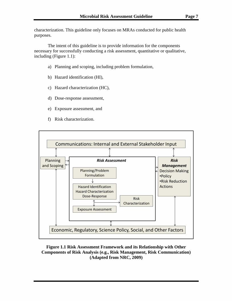
The intent of this guideline is to provide information for the components

necessary for successfully conducting a risk assessment, quantitative or qualitative,

including (Figure 1.1):

a) Planning and scoping, including problem formulation,

b) Hazard identification (HI),

c) Hazard characterization (HC),

d) Dose-response assessment,

e) Exposure assessment, and

f) Risk characterization.

Communications: Internal and External Stakeholder Input

Economic, Regulatory, Science Policy, Social, and Other Factors

Planning and Scoping

Risk Management

Decision Making•Policy•Risk Reduction Actions

Risk Assessment

Planning/Problem Formulation

Hazard IdentificationHazard Characterization

Dose-Response

Exposure Assessment

Risk Characterization

Figure 1.1 Risk Assessment Framework and its Relationship with Other

Components of Risk Analysis (e.g., Risk Management, Risk Communication)

(Adapted from NRC, 2009)


This guideline elaborates on these components that follow the Codex risk

assessment framework. However, the chapter order reflects the discussion of the

qualitative aspects of hazard characterization together with the qualitative aspects of

hazard identification. The quantitative aspects of hazard characterization (i.e., dose

response) are discussed in a separate chapter.

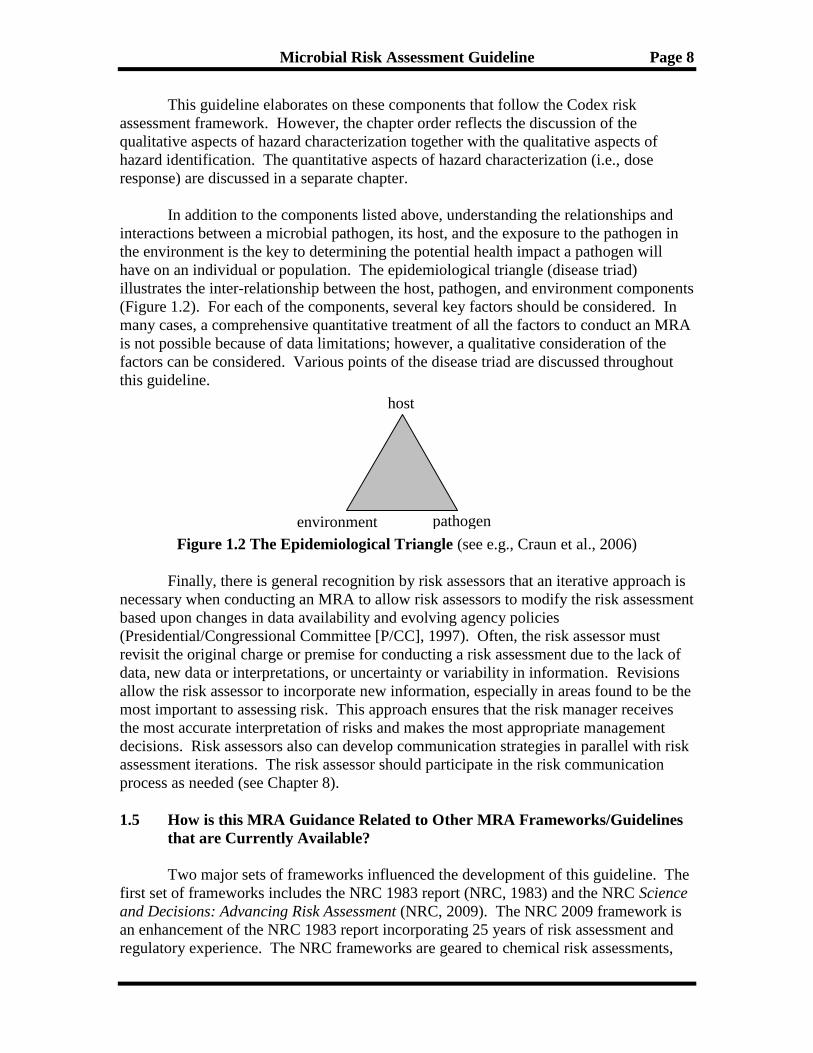
In addition to the components listed above, understanding the relationships and

interactions between a microbial pathogen, its host, and the exposure to the pathogen in

the environment is the key to determining the potential health impact a pathogen will

have on an individual or population. The epidemiological triangle (disease triad)

illustrates the inter-relationship between the host, pathogen, and environment components

(Figure 1.2). For each of the components, several key factors should be considered. In

many cases, a comprehensive quantitative treatment of all the factors to conduct an MRA

is not possible because of data limitations; however, a qualitative consideration of the

factors can be considered. Various points of the disease triad are discussed throughout

this guideline.

Figure 1.2 The Epidemiological Triangle (see e.g., Craun et al., 2006)

Finally, there is general recognition by risk assessors that an iterative approach is

necessary when conducting an MRA to allow risk assessors to modify the risk assessment

based upon changes in data availability and evolving agency policies

(Presidential/Congressional Committee [P/CC], 1997). Often, the risk assessor must

revisit the original charge or premise for conducting a risk assessment due to the lack of

data, new data or interpretations, or uncertainty or variability in information. Revisions

allow the risk assessor to incorporate new information, especially in areas found to be the

most important to assessing risk. This approach ensures that the risk manager receives

the most accurate interpretation of risks and makes the most appropriate management

decisions. Risk assessors also can develop communication strategies in parallel with risk

assessment iterations. The risk assessor should participate in the risk communication

process as needed (see Chapter 8).

1.5 How is this MRA Guidance Related to Other MRA Frameworks/Guidelines

that are Currently Available?

Two major sets of frameworks influenced the development of this guideline. The

first set of frameworks includes the NRC 1983 report (NRC, 1983) and the NRC Science

and Decisions: Advancing Risk Assessment (NRC, 2009). The NRC 2009 framework is

an enhancement of the NRC 1983 report incorporating 25 years of risk assessment and

regulatory experience. The NRC frameworks are geared to chemical risk assessments,

host

pathogen environment


but have applicability to MRAs. They also are broadly applicable for many different

exposure media. The second set of frameworks is the Codex Principles and Guidelines

for the Conduct of Microbiological Risk Assessment (Codex, 1999) and Codex Principles

and Guidelines for the Conduct of Microbial Risk Management (MRM) (Codex, 2007a).

The Codex framework is specific to food media, but is tailored to microbial hazards.

This guideline is broadly applicable to many media, but is tailored to microbial hazards to

humans. Both sets of frameworks were important for the development of this guideline.

These two sets of frameworks were not the only sources consulted for development of

this guideline.

U.S. government agencies (e.g., EPA, USDA, FDA, DHS, and DOD), as well as

government organizations from other countries (e.g., Canada, European Union, New

Zealand), and international agencies (e.g., WHO, FAO, Codex, and the Organization for

Economic Cooperation and Development [OECD] – for example, see FAO/WHO, 2003,

2006, 2008, 2009), have prepared various levels of guidance to support MRA

applications. An EPA-sponsored study, Foundations and Frameworks for Human

Microbial Risk Assessment (Parkin, 2008), presented an extensive search and evaluation

of frameworks available for use in conducting MRAs. The study identified four general

categories of frameworks applied in MRAs:

a) The 1983 NRC report;

b) A modified NRC 1983 approach without an explicit problem formulation (or

planning and scoping) step;

c) A modified NRC 1983 approach with a problem formulation (or planning and

scoping) step;

d) The International Life Science Institute (ILSI) approach (in association with the

EPA’s Office of Water) developed for water-based media (ILSI, 2000).

While most microbial risk assessors recognize shortcomings with a uniform,

exclusive application of the NRC 1983 approach, most have not explicitly attempted to

take a completely fresh look at approaches to conduct MRAs except for the ILSI (2000)

approach which was loosely based upon EPA’s draft Ecological Risk Assessment

Guidelines.

EPA, FDA, USDA, DOD, and DHS have utilized their own unique approaches to

conduct risk assessments, but it is important to keep track of other federally mandated

requirements that may apply to MRAs. For example, when relevant, Executive Orders

and OMB memorandums apply to MRAs (EPA, 2002b; OMB, 2007b; Presidential

Memorandum, 2009; OSTP, 2010).

1.6 What MRA Principles Should I be Aware Of?


While there are differences between chemicals and microbes (as detailed in

section 1.3), an MRA still adheres to the overarching principles for risk assessment in

general. Many documents contain pertinent principles, three of which are highlighted

here for MRAs (Codex, 2007b; EPA, 2000a; OMB, 2007b). Text Boxes 1.1, 1.2, and 1.3

provide a condensed version of the principles from these documents. For purposes of this

guideline, the principles are condensed to a few major points:

a) MRAs should be “fit for purpose” to address the appropriate risk management

problem(s)/issue(s).

b) MRAs should be as quantitative as possible. If quantitative data are not available,

a qualitative approach can be used to address the current risk issue(s).

c) MRA assumptions and uncertainties need to be considered, explained, and

documented.

d) Any MRA is developed using an iterative process, with each iteration increasing

the quality of the data in order to reduce uncertainties and/or refocus the scope.

The Office of Science and Technology Policy (OSTP) directs that “When

scientific or technological information is considered in policy decisions, the information

should be subject to well established scientific processes, including peer review where

appropriate, and each agency should appropriately and accurately reflect that information

in complying with and applying relevant statutory standards” (Presidential Memorandum,

2009; OSTP, 2010).

By addressing these principles and adhering to well established scientific

processes such as peer review, the correctness and the real world applicability of the

MRA is most likely ensured.

Text Box 1.1 General Principles of MRA Adapted from Codex (2007b)

Each risk assessment should be fit for its intended purpose.

Each risk assessment should state the scope and purpose clearly.

Experts involved in risk assessment should be objective and not be subject to any

conflict of interest that may compromise the integrity of the assessment. Information

on the identities of these experts, their individual expertise, and their professional

experience should be publicly available, subject to national considerations. These

experts should be selected in a transparent manner based on their expertise and their

independence with regard to the interests involved, including disclosure of conflicts

of interest in connection with risk assessment.

Risk assessments should use available quantitative information to the greatest extent

possible. It may also take into account qualitative information.

Risk assessments should consider constraints, uncertainties, and assumptions that

have an impact. Risk assessments should be based on realistic exposure scenarios.

They should include consideration of susceptible and high-risk population groups.


The risk assessment should be presented in a readily understandable and useful form.

Text Box 1.2 Principles of TCCR (Adapted from EPA, 2000a).

Transparency shows that the methods and assumptions are clear and understandable

(i.e., the use of methods, models, assumptions, and defaults are clear for others to

correctly follow and understand the MRA).

Clarity means the MRA is easy to understand and written in simple language.

Consistency provides a context to compare to similar documents/assessments.

Reasonableness explains founded and plausible professional judgments and

assumptions.

Other factors are also important for the MRA, such as the assessment of data

quality, data analysis, and peer review. Most agencies have addressed their needs for

these in separate agency guidelines, and all have adopted OMB Information Quality

guidelines relevant to these issues (OMB, 2002).

Text Box 1.3 Principles for Risk Analysis (adapted from OMB, 2007b)

Agencies should employ the best reasonably obtainable scientific information to

assess risks to health, safety, and the environment.

Characterizations of risks and of changes in the nature or magnitude of risks should

be both qualitative and quantitative, and consistent with available data.

Judgments used in developing a risk assessment should state assumptions, defaults,

and uncertainties explicitly.

Risk assessments should encompass all appropriate hazards including attention to

susceptible populations.

Peer review of risk assessments can ensure that the highest professional standards are

maintained.

Agencies should strive to adopt consistent approaches to evaluating the risk.

1.7 How can the MRA be Used?


Although risk assessments conducted by different agencies are not used for the

same purposes, agencies usually perform risk assessments with one or more of the

following goals in mind (adapted from U.S. Army Center for Health Promotion and

Preventive Medicine [USACHPPM], 2009). The goals could shape the planning and

scoping discussion (see Chapter 2) and ultimately the risk assessment. The goals are:

a) To mitigate (e.g., adverse effects or risk from a specific event);

b) To confirm (e.g., to determine if regulations, policies, standards, criteria, and/or

goals are adequate);

c) To decide whether and/or how to regulate (e.g., as needed to establish regulations,

policies, standards, criteria, and/or goals);

d) To investigate (e.g., to determine research or other requirements that would

enhance predictive and/or risk ranking capabilities, or facilitate completion of

screening or feasibility assessments).

1.8 What Are Examples of Types of MRA?

Risk assessments can take various forms depending on the agencies’ needs, risk

management issue(s), or the immediate problem at hand.

a) Screening – Screening assessments often provide a conservative, health-

protective estimate of possible risk that is based on the available data (this may be

thought of as a “simple” quantitative risk assessment). Risk assessors often

conduct screenings when a time critical decision is needed (e.g., quick mitigation

action is required after an event; imminent exposure to a microbial hazard is

identified). A risk assessor may resort to default assumptions to bridge data gaps

that cannot wait for research to fill. In addition, screening assessments may

actually provide the needed information that can address a risk management issue

without having to initiate a more data or model intensive risk assessment.

b) Risk ranking – Risk ranking assessments compare the relative risk among

several hazards. For example, this type of assessment might involve a single

pathogen associated with multiple foods, a single food that has multiple

pathogens, or multiple pathogens and multiple foods. Risk ranking assessments

can help establish regulatory program priorities and identify critical research

needs. The Food and Drug Administration/U.S. Department of Agriculture

(FDA/USDA) L. monocytogenes risk assessment is an example of a risk ranking

assessment (FDA/USDA/CDC, 2003).

c) Product pathway analyses – Product pathway assessments examine factors that

influence the risk associated with specific vehicle/hazard pairs. For food, it

ideally starts at the farm and ends with consumption. This type of assessment

technique helps identify the key factors that affect exposure including the impact


of potential mitigation or intervention strategies on the predicted risk. The FDA

Vibrio parahaemolyticus risk assessment is an example of a product pathway

analysis (FDA, 2005).

d) Risk-risk – Risk-risk assessments consider a trade off of one risk for another (i.e.,

reducing the risk of one hazard increases the risk of another). As an example, an

assessment could determine how treating drinking water with a chemical (risk to

disinfection by-product exposure) would impact public health versus the impact

of exposure to pathogenic organisms in water that is not treated.

e) Geographic – Geographic risk assessment examines the factors that either limit

or allow the risk to occur in a given region. The assessment examines risk of

introduction of disease agents through water, air, food animals, or animal products

in the United States (e.g., intentionally as in a bioterrorism act or unintentionally).

For example, the geographic approach might examine the risk of introduction of

bovine spongiform encephalopathy (BSE) into the U.S. cattle herds and the

subsequent risk of variant Creutzfeldt-Jacob Disease (vCJD) in humans by the

transmission from cattle through meats and animal products.

f) MRA within sustainability assessments – Using a systems-level assessment

over the lifetime of its technical components, sustainability assessments attempt

to account for human health, ecosystem health, and economic considerations. The

human health aspects include chemical and MRAs. This approach includes the

MRA over the expected lifetime of the technical system and via all exposure

pathways of pathogens to humans (e.g., drinking water, reuse waters, aerosols

pathways, recreational exposures, and contaminated soils/foods).

g) Threat and vulnerability assessments – Threat and vulnerability assessments

are specialized tools for evaluating the susceptibility of systems and facilities to

potential threats, such as adversarial actions (e.g., vandalism, insider sabotage, or

terrorist attack), natural disasters, and other emergencies. Although not strictly

speaking a “risk assessment,” the results can be similar where they identify threats

and characterize the nature, probability, and magnitude of adverse effects, and the

results can help to inform risk management decisions. For example, it may be

necessary to assess the risks associated with intentional contamination of the food

or water supply with biological agents or release of biological agents as an aerosol

into highly populated indoor or outdoor public areas. These assessments can

identify corrective actions that can reduce the risk or lessen the severity of

potential consequences. The CARVER plus Shock method (FDA, 2007) is a

preemptive targeting prioritization tool, which has been adapted for use in the

food sector.

1.9 What Types of Decisions within Risk Assessment are Science Policy?

Science policies, sometimes codified in an agency’s procedures, are used to aid

both the assessor and decision maker in the decision-making process. Science-policy


positions and choices are by necessity utilized during the risk assessment process in

two major ways. First, there are some basic, fundamental science-policy positions that

frame the risk assessment process to ensure that the risk assessments are appropriate

for a particular decision. These scoping “boundaries” for the risk assessment are

articulated during the planning and scoping process and ultimately explained clearly in

the risk characterization (i.e., what will be addressed in the risk assessment for

decision purposes, but also just as importantly, what will not be addressed and why

[e.g., not pertinent to the decision needed]). These science-policy positions not only

shape the risk assessment process, but are usually factors in the risk management

process outside the risk assessment.

Second, the use of default assumptions in a risk assessment is a science-policy

choice often invoked when there is a lack of data. These choices are more specific than

the framing science policies mentioned above. Given the nature of uncertainty and data

gaps, default assumptions (sometimes simply called defaults) address these uncertainties

when data are unavailable or otherwise not suitable for use. A default assumption is the

best option available in the absence of data to the contrary (NRC, 1983). The NRC

supports the use of default assumptions in its review of risk assessment practices in

Science and Judgment in Risk Assessment (NRC, 1994). The report also stated that

agencies should have principles for choosing default options.

When pathogen-specific data are unavailable (i.e., when there are data gaps) or

insufficient to estimate parameters or resolve paradigms, a default can be used in order

to continue with the risk assessment. This is a science-policy choice, generally agreed

upon during the planning and scoping discussions, when data gaps are identified (see

section 2.4.4 for information on data gaps). During the risk assessment itself, a default

is used only when essential data are lacking. Point estimates also can be considered

defaults when the distribution of the parameter adds unnecessary complexity given the

needs of the risk assessment. For example, drinking water consumption is often

modeled probabilistically for MRAs with a median of 1liter per day. The consumption

value of 2 liters per day per person is often used for chemicals and represents the 90th

percentile of the 1994 to 1996 and 1998 Continuing Survey of Food Intake by

Individuals community drinking water consumption data. As illustrated in this example,

the choices you make need to be well within the range of plausible outcomes and often

at specific percentiles (for variability) within that range of observation. The use of 1liter

versus 2liters/day is not related to differences in microbial versus chemical risk

assessment.

The default assumptions are not pathogen-specific per se, but are relevant to the

data gap in the risk assessment. Defaults are based on published studies, empirical

observations, extrapolation from related observations, and/or scientific theory. Appendix

A of this volume provides a representative list of assumptions commonly made.

Beyond these two ways, this guideline does not address the types of policy or

regulatory decisions that occur after the results of the risk assessment have been


considered. Science-policy decisions are differentiated from scientific judgment calls.

Whereas risk assessors can make decisions based on scientific judgment, if a decision

goes beyond what would reasonably be considered firmly supported by science, then

policy comes into play. Once policy is involved, then risk managers need to become

engaged in the decision-making. Failing to distinguish between policy decisions and

scientific judgment in a risk assessment is a serious threat to the scientific credibility of

the assessment. It is important to note that:

a) The utilization of science policy in the risk assessment process is not meant to

“bury” or “hide” risk management decisions within the risk assessment. The use

of a science-policy position or choice in the risk assessment process does not

direct the risk assessment itself toward a specific risk management decision.

b) To be transparent, the risk assessment should state policy choices explicitly.

c) The policy positions themselves are developed outside the risk assessment.

Scientific data should support science-policy positions, and risk assessors and risk

managers should ensure that the risk assessment proceeds in a way that provides the most

accurate information for decision-making.

1.10 Why are Uncertainty and Variability in MRA Important?

According to the NRC, characterizing uncertainty and variability is key to the risk

assessment process (NRC, 2009). The NRC provided recommendations on use of

defaults, methods for, if possible, quantifying uncertainty, and how to consider variability

in exposure and susceptibility. The NRC defines regarding uncertainty and variability

in risk assessment (NRC, 2009):

Uncertainty: Lack of or incomplete information. Quantitative uncertainty analysis

attempts to analyze and describe the degree to which a calculated value may differ

from the true value; it may use probability distributions. Uncertainty depends on

the quality, quantity, and relevance of data, as well as the reliability and relevance

of models and assumptions.

Variability: Variability refers to true differences in attributes due to heterogeneity

or diversity. Variability is usually not reducible by additional measurement or

study, although it can be better characterized.

Almost every aspect of a risk assessment will have some level of uncertainty,

usually due to data gaps and incomplete knowledge. Variability is a natural part of

biological systems and will always exist. Often variability cannot be reduced, but it can

be better understood with more information and knowledge. Both of these aspects are

discussed in the risk assessment, and the degree of uncertainty and variability are

characterized and quantified, if possible.


This guideline discusses ways to address uncertainty and variability (e.g., use of

defaults, quantitative uncertainty analysis, sensitivity analysis, use of expert elicitation, or

probability distributions). While there are techniques available to perform these analyses

(e.g., two-stage Monte Carlo analyses), such analyses are not always necessary to address

the particular risk management questions/issues at that moment. The “depth” or level of

detail of these analyses can be discussed, particularly during the planning and scoping

phase of risk assessment (e.g., see section 2.3).

1.11 Summary

This guideline is applicable to a wide array of scenarios but focuses on

microorganisms that are capable of causing infection and disease in humans.

Specifically, it is applicable for assessing risk associated with ingestion of foodborne

pathogens (e.g., raw and processed foods), and water-based or waterborne pathogens

(e.g., drinking water, recreational water, wastewater). Risk assessors could apply these

guidelines to assess risks of human exposure to biological warfare agents or pathogens in

soil, solid wastes, or air. This guideline also may apply to other common forms of

exposure, including inhalation and dermal exposure pathways. At present, this guideline

does not cover oligonucleotides, prions, preformed microbial toxins, and other

submicrobial entities owing to a wide array of unknowns associated with those agents.

This guideline accounts for differences between the general population, different

life stages, and sensitive populations. It is flexible to allow risk assessors to address risks

to individuals, populations, and the general population using either available static or

dynamic susceptibility models. This guideline provides approaches and tools appropriate

for typical human health related concerns. The guideline does not include criteria to

identify sensitive groups or life stages, because those groupings are specific to each risk

assessment, based on the agencies’ unique health protection concern and public health

goal.

This guideline facilitates systematic and transparent consideration of relevant

factors that impact the risk assessment and facilitates reproducible risk evaluation. This

process allows agencies assessing a similar medium or pathogen to compare and contrast

the details and assumptions of their assessment to another agencies’ assessment. This is

not to say that each risk assessment will be completely cross-comparable, because there

are a number of specific data sources and agency requirements that require different

inputs and applications. The differences in requirements are why this guideline is

designed to be modular and able to provide flexibility for each agency’s specific

requirements. On an international scale, there also is a need to have common approaches

to an MRA to effectively satisfy international trade agreements and public health

protection for importation of food and beverage products and assess international risks

from emerging pathogens around the world. This guideline is harmonized with both the

NRC and Codex frameworks.


2. PLANNING AND SCOPING

Planning and scoping ensures that a risk assessment is relevant and well done.

The NRC 2009 framework recommended “increased attention to the design of risk

assessment in its formative stages [and] that planning and scoping and problem

formulation, as articulated in EPA guidance documents (EPA, 1998a, 2003a), should be

formalized and implemented in EPA risk assessments” (NRC, 2009). Rigorous

preparation is needed at the start of the risk assessment process to facilitate

communication during and following the risk assessment and to ensure that all issues are

sufficiently vetted, all participants are clear on the objectives and goals, and managers are

clear about the commitment of personnel and other resources (EPA, 1992; NRC, 1996).

To obtain detailed descriptions of the usefulness and implementation of the

planning and scoping process, the FDA, USDA, and EPA provide general information on

how to proceed (FDA, 2002; USDA, 2003a; EPA, 2000a, 2002a; NRC 2009). This

chapter provides an overview of this first step in the risk assessment process. Several

interesting case studies from ecological risk assessment are presented in EPA’s Lessons

Learned on Planning and Scoping for Environmental Risk Assessments (EPA, 2002a).

2.1 What is Planning and Scoping?

Planning and scoping is a

process that defines the purpose and

scope of a risk assessment and focuses

the issues and approach(es) involved

in performing the assessment. A

clearly articulated purpose and scope

provides a sound foundation for later

judgments on the success of the risk

assessment and for an effective risk

characterization. In a sense, the

planning and scoping process lays out

a “road map” for how the risk

assessment will be accomplished (Text

Box 2.1).

The planning and scoping

process helps all parties involved in

the risk assessment understand how

the risk assessment fits into the overall

decision-making process. Planning

and scoping promotes:

a) Identification of appropriate timelines and needed resources, thereby improving

efficiency;

Text Box 2.1. Planning and Scoping (based

on EPA, 2003a, 2004a; NRC, 2009)

Planning and scoping involves:

Defining the purpose of the assessment

Defining the scope of analysis and products

needed

Agreeing on participants, roles, and

responsibilities

Agreeing on depth of assessment and

analytical approach (e.g., will the risk

assessment include static or dynamic

modeling)

Agreeing on resources available and

schedule

Formulating the problem

Developing the conceptual model

Constructing the analysis plan

Identifying initial risk management options

that are available


b) agreement among principle parties on realistic expectations regarding the goals,

commitment, time-frame, and resources;

c) the prospect of less unanticipated controversy, because all interested parties

contribute and disagreements can be dealt with swiftly and not left as a surprise at

the end;

d) identification of and participation by those from many disciplines (e.g.,

microbiologists, toxicologists, economists, lawyers) to help in the process thereby

ensuring that each risk assessment and characterization is useful for the intended

audience(s);

e) an understanding of the degree of complexity needed in the risk assessment to

adequately inform the decision at hand; and

f) informed decisions with stakeholder buy-in.

2.1.1 What is Problem Formulation?

At the beginning of the risk assessment, and frequently within planning and

scoping, a problem formulation exercise frequently occurs. It is a discussion and analysis

activity that focuses the technical/scientific aspects of the issue at hand. All relevant

parties, including the risk manager, risk assessment team, risk communication specialist,

and, when appropriate, relevant stakeholders and interested parties, participate. Problem

formulation usually provides:

a) A definition of the valued entity and endpoint: what is the entity that should be

protected and what are the undesirable effects that you are trying to avoid. For

MRA this may involve a policy determination of what the “valued entity” is (e.g.,

general population, young children, pregnant women, immunologically

compromised) and what is considered to be an appropriate level of protection

(ALOP) against infection or disease.

b) A conceptual model that lays out the anticipated exposure scenarios of the

microorganisms from the source to the receptor. With an MRA, this may be the

movement of enteric pathogens from a source (e.g., treatment works, manure

application to a field, critical point in the food processing system) to the

population of concern. It highlights various hazardous events that may lead to

increased risk and where risk management may be most effective.

In some cases, a valid conceptual model may be unavailable, or there may be

multiple plausible, but distinct conceptual models. The validity of a selected

conceptual model may simply be uncertain. The risk assessor should be aware of

these possibilities and may need to consider multiple (and uncertain) conceptual

models as well as possibly model-free (e.g., source tracking) methods as part of

the formulation.


c) An analysis plan provides a road map for addressing the problem. In short, it is

analogous to an experimental design. In the analysis plan, risk hypotheses

generated earlier are examined and discussed; the relationships between pathways

and valued entities are further examined. The level of precision and data quality is

considered in light of available information. The analysis plan may not be

restricted to only pathway-based approaches because all important pathways may

not be known with confidence.

It is important in problem formulation to identify as many possible (more

importantly, probable) outcomes and their consequences. Also, unintended consequences

should be identified where possible and addressed as part of the scope of the MRA (e.g.,

do possible interventions targeted at reducing one pathogen run the risk of increasing

illnesses from another pathogen, or do the mitigation strategies themselves have risks

[e.g., disinfection byproducts]). During the problem formulation activity, a “bad”

formulation could ultimately restrict the value of the subsequent risk assessment.

2.2 What do I Consider When Deciding to Initiate an MRA?

Unless your agency is required to conduct a particular risk assessment (e.g.,

statutorily mandated), managers need to decide whether a risk assessment is appropriate,

feasible, and will actually be performed. This decision is commonly made during

planning and scoping. The agency may decide not to initiate a risk assessment after the

planning and scoping step because a decision can be reached without conducting a risk

assessment. Several criteria to consider for identifying a candidate risk assessment

include:

a) Characteristics and importance of the hazard(s) of concern;

b) Magnitude (e.g., presence, prevalence, concentration of hazards) and severity

(e.g., impact on public health) of the risk;

c) Urgency of the situation;

d) Populations of concern;

e) Other factors associated with specific hazards (e.g., water treatment processes,

food processing, cooking, cross contamination);

f) Availability of resources (e.g., time, money, staff).

A diversity of ideas at the planning and scoping stage is important for exploring

the range of possibilities (i.e., whether a risk assessment is truly needed to what type of

risk assessment may be necessary). It is also important not to focus on one aspect too

soon during planning and scoping as that may not be the “best” or “correct” way to

proceed.


Whether a risk assessment may be

required to comply with regulatory

analysis requirements (OMB, 2003) is

another consideration to take into account

during planning and scoping. The Office

of Information and Regulatory Affairs has

provided a checklist to assist agencies in

producing regulatory impact analyses

(RIAs), as required for economically

significant rules by OMB Circular A-4

(OMB, 2010; OMB, 2003). Appropriate

assessments of risk may be necessary to

address international trade agreements

(e.g., World Trade Organization Sanitary

and Phytosanitary Agreement). Ensuring

that each assessment of risk is fit for its

intended purpose and is based on scientific

data most relevant to the national context

ensures that the effort and scope of the

assessment of risk are appropriate for the

risk management questions being raised so

that practical risk management options can

be formulated.

Text Box 2.2 provides a list of examples of when a risk assessment may be appropriate.

Text Box 2.3 provides FDA Center for Food Safety and Applied Nutrition’s (CFSAN)

process for selecting risk assessment topics.

Text Box 2.2 Examples of when a risk

assessment may be appropriate.

Review of the reliability or utility of a

standard

Cases where the current standard is

inconsistent with other government

policies, guidelines, or thresholds

Cases where an agency has been

petitioned for a regulatory action

Establishment of standards for

regulatory action

Evaluation of the public health

implications of different tolerable risk

levels

Cases where a data gap analysis is

desired

Cases where the hazard is a serious

health issue, emerging pathogen, and/or

public health concern

The exposure system is complex.


Text Box 2.3 FDA CFSAN’s four phases for selecting, conducting, and

communicating food safety risk assessments (FDA, 2002).

Phase 1: Concept Generation – Collect ideas and maintain a list of potential risk

management questions for which a risk assessment would assist with policy

decisions. Develop justification for candidate risk assessments, including purpose of

assessment, scope of problem, importance to the Center, and use of the result by the

Center.

Phase 2: Problem Identification – The candidate risk assessment and supporting

information (justification) are reviewed to determine whether the assessment meets

the Center’s needs. This phase results in one of three recommended actions, conduct

data feasibility study, not required for regulatory decision, or more information

needed to make decision.

Phase 3: Data Feasibility (Evaluation and Recommendation) – Information is

collected and reviewed to determine availability of data needed to answer risk

assessment question(s). This phase results in one of four recommended actions,

conduct quantitative risk assessment, conduct qualitative risk assessment, more

research needed, or modify question and conduct alternative assessment.

Phase 4: Disposition (Selection) – Using the results from the data feasibility

determination as an aid, risk assessment(s) to be conducted are selected. Decision is

based on technical merit, resource availability, the Center’s priority needs, and other

legitimate factors.

2.3 What “Depth” Can I go into in the Risk Assessment?

Once a decision is made to initiate a risk assessment, a major consideration for the

risk assessment approach is how much detail or “depth” to incorporate to address the risk

management question(s) or decision. Due to various management needs, the risk

assessment approach is not necessarily one-size-fits-all. This guidance is intended to

provide flexible methods for supporting different types of assessments (e.g., screening,

safety) and outputs (e.g., qualitative or quantitative), as described in Schaffner (2008).

Guidance from Codex (1999) and World Organization for Animal Health (OIE, 1999)

described qualitative and quantitative outputs as equally valid (Wooldridge, 2008).

Wooldridge (2008) provides detailed discussion of qualitative and quantitative

assessments, and other risk analysts (Dennis et al., 2008) discuss both estimates of risk

and safety, mortality for listeriosis, and allowable ('safe') levels of Vibrio in seafood,

respectively.

Be aware that the terms referring to the different types of assessments are

specifically defined in different contexts; care should be used when “naming” or referring

to types of assessments. For example, this guideline is specific to the selection and

conduct of risk assessment, not a safety assessment. One difference is that risk


assessment estimates the likelihood and/or frequency of adverse health outcomes

resulting from an exposure and, in some cases, sources of risk. It also deals with

quantitative reductions in risk based on various interventions. While much of this

guideline is relevant to a safety assessment, a safety assessment may estimate the

likelihood and/or frequency of exceeding a specified threshold of concern (e.g.,

predetermined regulatory limits or standards) or provide a determination of what is “safe”

based on the conventions of the standard-setting procedure. For example, Codex

standards traditionally specify maximum limits for additives and residues in foods based

on the concept of “no appreciable risk” (FAO/WHO, 1997). For contaminants in foods,

the Codex standards are based on the concept of “as low as reasonably achievable”

(FAO/WHO, 1997). Risk-related terms in some statutes have formal definitions. The

risk assessor should be aware of statutory definitions that apply to a risk assessment.

There are many cases when a screening risk assessment is preferable over a fully

developed risk assessment (see section 1.8 for screening definition). It is important to be

transparent about the amount of uncertainty in the screening estimate and discuss whether

the uncertainty causes underestimates or overestimates of risk based on the assumptions

applied. This work may be followed by a more detailed assessment that will need to be

conducted or risk managers will need to take action(s). The risk assessor may return to

the assessment to refine and recalculate estimates based on additional data (e.g., quick

sampling assays, use of surrogate data, expert elicitation). Alternatively, there may be a

risk management decision to conduct a full risk assessment.

A comprehensive (“major”) risk assessment requires a substantial commitment of

resources. Thus, this depth of risk assessment is not necessary when risk managers do

not need this level of sophistication to make a decision. Circumstances that may not

warrant a quantitative risk assessment would include, for example, a risk that is well

described by definitive data, a problem that is relatively simple, or an issue that is not of

regulatory concern. However, a comprehensive risk assessment is a powerful tool to help

risk managers evaluate and interpret information when the data describing a hazard are

incomplete, the exposure system is complex, or the issue is of high regulatory or

stakeholder concern.

Risk assessments can be either qualitative or quantitative (or parts of each, e.g., as

in “semi-quantitative”) in their description of the likelihood of adverse health effects,

depending on the extent of the data and knowledge available, the existence of models or

other tools for quantitative predictions, the complexity of the problem, the scope and

nature of the question(s) posed by the risk managers, and the time available to conduct

the assessment. In quantitative assessments, the risk is expressed as a mathematical

statement of the probability of illness or death after exposure to a specific hazard, and it

represents the cumulative probabilities of certain events happening and the uncertainty

associated with those events. Conversely, qualitative risk assessments use verbal

descriptors of risk, severity, and uncertainty, and often involve the aggregation of

assumptions.


Text Box 2.4 Products of Planning

and Scoping

Statement of Concern

Statement of Purpose and Objectives

Background Section

Scope

Scenarios

Literature Review

Data Inventory

Tools and Methods Inventory

Risk Management Questions or Charge

Risk Profile

Conceptual Model

Value-of-information analysis

Communication Plan

Analysis Plan

Work Plan

Data Quality Objectives

2.4 What Elements are Discussed

During Planning and Scoping?

Various elements are discussed

during planning and scoping. Not all of these

elements are necessary for every risk

assessment, and certain elements will be

more appropriate for a particular problem.

Examples of products of planning and

scoping are listed in Text Box 2.4 and

underlined in the text where the elements and

activities of planning and scoping are

described. Not all of the elements and

activities that occur during planning and

scoping have associated written products.

This section begins with an overview of the

elements and activities of planning and

scoping, and then provides more detail for

selected elements as third level header

questions and answers.

Principal outputs from planning and scoping can include various products that are

appropriate to the management objectives and the plan for analysis of the risk. The level

of deliberation and content of the outputs vary depending on the complexity required for

the assessment. Further, some outputs can be contained in other products (e.g., the risk

profile document can contain many of the listed products). You need to discuss what

outputs will be generated during the planning and scoping deliberations. In general,

many of these products are good candidates for peer review. Peer review or consultation

early in the risk assessment process can provide timely insights, corrections to

assumptions, and directions on proper ways to proceed during the risk assessment.

During planning and scoping, participants can engage in a dialogue to answer the

following questions and commit to the outcome of those discussions to facilitate mutual

understanding (elements underlined):

a) What is the motivation for the risk assessment? A Statement of Concern

relays a common understanding of what broad issue the risk assessment will

address. Describe in simple terms what hazard is being addressed and how it is

thought to relate to human health for an exposure scenario. Include any other

driving factors for the risk assessment, such as a food safety issues, regulatory

requirements, public concern, or new scientific findings.

b) What are the management goals, issues, questions, and policies that need to

be addressed? A Statement of Purpose and Objectives is a concise paragraph

that addresses the management goals. The management questions are designed to

provide the information needed for decision-making. It is in the best interest of

all parties involved (e.g., assessors, managers and decision makers, stakeholders)


to state, at the outset, the question(s) that needs to be answered in the assessment

explicitly.

c) What is the context of the risk assessment? Risk assessments are done in

historical and social contexts. A Background Section summarizes any previous

risk assessments that addressed the same or similar hazards. A risk assessor can

use a previous risk assessment to summarize the relationship between the current

and previous risk assessment. The context of a risk assessment may include

different mandates, regulatory requirements, policy developments, or information

derived from technical advancements, risk assessment method and tool

advancements, and new or enhanced data sets.

d) What is the scope and coverage of the risk assessment? The Scope outlines the

scenarios the risk assessment will cover. Answering the scoping questions below

can ensure the information regarding scope is necessary to conduct the MRA.

1) Which infectious disease hazard is being addressed (pathogen strain[s],

indicator[s], or taxon [genus, species, strain/biovar])? Define the hazard.

2) Which human populations will be the focus of the risk assessment (e.g.,

general population, life stages, or geographically defined populations)?

Describe which populations are explicitly included in the risk assessment

model, which populations will be accounted for implicitly, and which

populations may be excluded by the risk assessment model (e.g., most

extreme behaviors).

3) What health outcomes or endpoints are addressed by the risk assessment,

and how is the health outcome measured? Clearly defining the health

endpoint is important for transparency and focuses the scope of the risk

assessment (e.g., infection, disease symptom[s], mortality).

4) What unit and routes of exposure are relevant and why? Determine the

time-span of exposure relevant to the decision.

5) For risk assessments designed to derive nominally or presumptive “safe”

levels of microorganisms (i.e., levels below a threshold of regulatory

concern), what level of protection will be provided, and what is the technical

or policy justification for that level? Transparency in public health

objectives is important.

6) What specific exposure scenarios should be modeled? List specific scenarios

the risk managers would like to model (varying the inputs), including

desired spatial and temporal features.

e) What type of risk assessment is needed to address the risk management

question(s)? Section 1.8 describes different types of risk assessments, including

screening, risk ranking, product pathway, risk-risk, geographic, systems-level

(sustainability risk assessment), and threat and vulnerability assessments.


f) What is the state of the current knowledge? The planning and scoping can

include an overview of current knowledge and be used to outline the topics that

will be reviewed in more depth in the rest of the risk assessment. A Literature

Review provides understanding of the current state of the science.

g) What and where are the available data? In addition to identifying the available

data, a Data Inventory addresses data relevance, data use, data accessibility, and

data quality. An inventory may also provide notice to the public of the data

currently available to the agency in a call for data. In addition to literature

searches, government databases provide data that are useful for risk assessments.

For example, WHO maintains the Global Health Observatory Data Repository,

the Centers for Disease Control and Prevention (CDC) conducts the National

Health and Nutrition Examination Survey (NHANES), as well as the FDA and the

University of Maryland’s Joint Institute for Food Safety and Applied Nutrition

sponsors foodrisk.org.2 See section 2.4.6 for further discussion of data quality.

h) How do I know what questions the risk assessment needs to answer? The

Risk Management Questions or Charge are usually written down and discussed

iteratively between the risk assessment team and risk managers to ensure common

understanding of the questions. See section 2.4.1 for discussion on risk

management questions and charge.

i) What are the information/data needs of other members of the “team?” The

risk assessment may be part of a larger project, such as an economic analysis.

There may be economic, social, or legal analyses that need to be coordinated with

the risk assessment.

j) How will you model the risk? A Tools and Methods Inventory typically

includes statistical methods for estimating model inputs and tools for addressing

uncertainty and variability and should make an initial determination of which

methods and tools are likely to be most useful. It is advised that models used in

the risk assessment be peer reviewed preferably before starting the risk

assessment. Software needs should also be considered; some risk assessment

software tools include Oracle’s Crystal Ball, Palisade Corporation’s @Risk,

Berkeley Madonna, and Lumina Decision System’s Analytica. EPA’s

Compendium of Prior and Current Microbial Risk Assessment Methods for Use

as a Basis for the Selection, Development, and Testing of a Preliminary Microbial

Risk Assessment Framework has citations for many tools (EPA, 2007c).

k) What are possible risk assessment or risk management options? Particularly

for risk assessments that are needed to evaluate intervention strategies or needed

to support regulatory determinations, different options should be presented as

different scenarios for the risk assessment. Those Scenarios should be clearly

stated during problem formulation and may evolve during risk assessment

iterations.

2 http://apps.who.int/ghodata/ ; http://www.cdc.gov/nchs/nhanes.htm;http://foodrisk.org/

http://apps.who.int/ghodata/

http://www.cdc.gov/nchs/nhanes.htm

http://foodrisk.org/


l) What are the logistical considerations for conducting the risk assessment? The Analysis Plan (see section 2.4.5) or a Work Plan contains logistical

considerations. These include:

1) resources available to do the assessment, including funding and staff time;

2) participants in the process and their roles;

3) plans for coordinating across offices, with other agencies, and with

stakeholders; and

4) scheduling (e.g., milestones, deliverable due dates, quality audits, meetings),

including provisions for timely and adequate internal, independent external

peer review, and if required, interagency review.

m) How will planning activities and results be communicated to senior managers

and to the public? Chapter 8 discusses risk communication within the context of

risk assessment.

n) What are the legal considerations and constraints that may shape the

ultimate decision and supporting risk assessment? The technical office

conducting the risk assessment can engage the agency’s legal department,

according to normal practices within that agency. The Background Section

discusses legal and statutory context.

o) How and at what iterations will the risk assessment be peer reviewed?

OMB has published Information Quality Bulletin for Peer Review, which

provides general peer review guidance and sets minimal expectations for the

review of scientific information (OMB, 2004). Most agencies have agency

specific peer review guidance that complies with the OMB guidance. Follow

your agency’s peer review guidance. For example, EPA’s Peer Review Handbook

(EPA, 2000c, 2006c) provides guidance on selection of peer reviewers that

includes where to find peer reviewers, what mix of expertise may be important,

representing diversity of disciplines, and limiting conflicts of interest. According

to the National Committee on Radiation Programs (NCRP, 1996), an expert has

the following characteristics:

1) training and experience in the subject area resulting in superior knowledge

in the field;

2) access to relevant information;

3) an ability to process and effectively use the information; and

4) is recognized by his or her peers or those conducting the study as qualified

to provide judgments about assumptions, models, and model parameters at

the level of detail required.


The following sub-sections flesh out some of the major elements iterated above.

2.4.1 What are Risk Management Questions and What is the Charge?

Section 2.4 (above) presents a brief description of management questions.

Generating specific risk management questions for a risk assessment helps formulate a

clear, focused charge that identifies the technical and scientific issues on which you need

to address and suggestions for conducting the risk assessment. Formulating these

questions usually requires significant interaction between risk assessors and risk

managers, as well as dialogue with appropriate other parties (e.g., those with relevant

information about the potential hazard). The questions generated will focus the risk

assessment to provide the appropriate analyses to inform the risk management decision at

a level of detail appropriate for the issue. The resulting risk assessment can be designed

to address and answer as best as possible the risk management questions posed.

The charge focuses the assessment by presenting specific questions and concerns,

including the comprehensiveness of the data, information, and literature, the soundness of

the methods proposed, the scientific support for the assumptions employed, and the

sensitivity of the results to possible alternative assumptions. In general, time is well-

spent preparing a good set of questions or a charge, which are crucial for an effective risk

assessment and ultimate decision. In this context, the charge is the set of questions and

does not imply a formal charge.

2.4.2 What is a Risk Profile?

Codex defines a risk profile for food safety as: “a description of a food safety

problem and its context that presents in a concise form, the current state of knowledge

related to a food safety issue, describes potential microbiological risk management

options that have been identified to date, when any, and the food safety policy context

that will influence further possible actions… Consideration of the information given in

the risk profile may result in a range of initial decisions, such as commissioning a

microbiological risk assessment, gathering more information or developing risk

knowledge at the level of the risk manager, implementing an immediate and/or temporary

decision” (Codex, 2007a).3 A typical risk profile includes: a description of the situation,

product, or commodity involved; information on pathways by which consumers are

exposed to the microorganism; possible risks associated with that exposure; consumer

perceptions of the risks; and the distribution of possible risks among different segments

of the population. For a list of information that Codex recommends including in a risk

profile see Codex (2007a).

A risk profile assists in identifying the risk management questions that need to be

addressed. The risk profile should be clearly and thoroughly documented, so that risk

managers can use it to decide on further action in relation to a specific health issue. If

3 “Risk profile” is sometimes used to refer to summary information at the end of each chapter in

frameworks based on the ecological risk assessment framework.


links are made between risk profiles for other risk assessments, risk profiles can provide

the basis for qualitative ranking of problems for subsequent risk management.

Notably, risk profiles can be used as decision tools that do not lead to risk

assessment. For examples, see the New Zealand Food Safety Authority.4

2.4.3 What is a Conceptual Model?

A conceptual model is a written or visual representation of predicted relationships

between the hazard and exposed populations.5 It is based on problem formulation and

working hypotheses; it is supported by preliminary data and information and used to

organize the conduct of an MRA.

The conceptual model depicts the movement of the hazardous agent from the

source to the host. Other tiers of conceptual models may identify variables and data

needed to conduct the MRA. A conceptual model (e.g., a source-pathway-receptor

model; “farm-to-fork” model) can be developed early in the planning and scoping

process, to the level necessary to address the risk assessment’s purpose. In some cases, a

pathogen may be available in multiple media and cause different diseases depending on

the route of exposure. During planning and scoping, the risk assessor can assess the

medium, pathway of exposure, and route of exposure. An example of a conceptual model

is provided in Figure 2.1. Other examples of conceptual models can be found in Suter

(1999).

Developing a sound and useful conceptual model may require several iterations.

The conceptual model describes or visualizes the relationships among the assessment and

measurement endpoints, the data required, and the methodologies that will be used to

analyze the data. An overall high-level conceptual model as well as more detailed

conceptual models that cover just dose-response or exposure assessment components may

be useful (EPA, 1998a). Overall, the purpose of a conceptual model is to enhance the

documentation of the risk assessment so that readers will have a clearer picture of the risk

assessment.

4 http://www.foodsafety.govt.nz/science/risk-profiles/

5 The conceptual model in planning and scoping differs from conceptual models that are used to map how

parameters are related in modeling software. The term conceptual model is used in both contexts in this

Guideline.


Figure 2.1 Conceptual Model for the “in-plant” component of the Listeria

risk assessment (from USDA 2003b).

2.4.4 How are Data Gaps Identified and Addressed in the Context of

Planning and Scoping?

Incomplete information and data gaps are a significant challenge throughout the

risk assessment discipline. Much of the “art” in risk assessment involves the judgments

regarding incomplete data and data gaps. In addition to missing data, risk assessors must

assess whether available data are representative of the actual conditions.

The extent to which a data gap exists is ultimately a matter of scientific judgment

within the context of what is an acceptable level of confidence. Different assessors and

managers may have different comfort levels for making decisions based on the same data.

In some cases, there may be differing options about how representative the data are and

whether the data adequately fit in the risk assessment scenario. The risk assessor must


consider the quality of existing data when determining if a data gap exists. To reduce the

heterogeneity of comfort levels, many different systematic schemes for evaluating data

quality, completeness, and applicability have been developed. Statistical approaches are

standard for evaluating data quantity, but still require a judgment about the appropriate

confidence level for decision-making. If the risk assessors and risk managers on your

team cannot agree on what constitutes a significant data gap, the team may need to take a

step back and first agree on criteria for evaluating data. With some data gaps, risk

managers look to risk assessors to tell them whether the data are sufficient, while risk

assessors may claim that a policy decision needs to be made by the risk managers

regarding setting the threshold for sufficiency. These types of situations can stall a risk

assessment, but ultimately the group has to reach agreement on the judgment call or

policy decision. If the existence of a data gap is not obvious and agreed upon easily, the

risk assessors and managers should document the evidence used to support the

identification of the data gap.

Stakeholders may have strong opinions about data gaps. Some may demand a

decision in the absence of data, while others may interpret the goal of science-based

decision-making to mean that more data must be available to make a decision. Robust

planning and scoping should be able to predict which data gaps have the potential to

cause the most debate.

Every parameter in the risk assessment will have some level of incomplete

information. Ranking the importance of the data gaps can help focus resources on the

most critical data gaps that, if filled, could influence the risk assessment results the most.

If there is more than one data gap, it may be critical to examine the set of gaps and their

possible interdependence when deciding how important the gaps are to the risk

assessment. The risk assessment results can be evaluated by conducting sensitivity

analysis (sections 5.3.3 and 6.6) or value-of-information (VOI) analysis (section 2.4.7) to

determine whether the data gap is significant. Determining data gaps and the relative

importance of different data gaps will progress iteratively as the risk assessment is

conducted.

Once a data gap (or set of gaps) is identified and determined to be important, it

can be a matter of scientific judgment or a policy decision that determines how the data

gap(s) will be addressed in the risk assessment. Use existing data in the near term to fill

information needs; in the midterm, conduct tests with currently available test methods to

provide data on the topic of interest. Over the long term, develop better, more realistic

understandings of exposure and effects and construct more realistic test methods to

evaluate pathogens of concern. In cases where an aspect of risk is likely to be important

but insufficient data are available, highlight the deficiency or use judgment or assumed

values to approximate the missing data (see section 6.4 for further discussion). The risk

assessor should clearly describe the judgments and approximations, and the implications

explained in the risk characterization.

OSTP states in their scientific integrity memo that, “The accurate presentation of

scientific and technological information is critical to informed decision making by the


public and policymakers. Agencies should communicate scientific and technological

findings by including a clear explication of underlying assumptions; accurate

contextualization of uncertainties; and a description of the probabilities associated with

both optimistic and pessimistic projections, including best-case and worst-case scenarios

where appropriate” (OSTP, 2010).

Depending upon the circumstances, the utility of a risk assessment may be

compromised if important policy decisions are put on hold while waiting for more

research results. Risk assessors and risk managers need to balance the need to obtain

more data/information against the need to make a timely decision. The data gaps

identified in planning and scoping may be very useful to establish a research program

and/or agenda to address current data gaps.

When data or information are lacking, expert opinion or judgment is an

alternative source of information, particularly used in exposure assessments. If no other

empiric evidence is available, expert judgment may offer insights to inform a model for

example. On the other hand, when data are completely absent and the availability of

expert opinion or judgment is questionable, it is possible to avoid the need for such data

by model simplification (Cox, 2006; Vose, 2008). Such an approach is particularly

worthwhile when empiric evidence is available to inform the probability distributions of

process outputs subsequent to the process that is missing data. Such ‘downstream’ data

(i.e., between the missing element and the ultimate exposure distribution) actually reflect

the likelihood of microbe levels given the processes (e.g., modeled or missing) that

occurred prior to the process. Therefore, processes for which data are missing may

effectively be skipped over if data are available downstream.

Methods for eliciting expert judgments have been suggested (Kaplan, 2000;

ECSCC, 2003). Ouchi (2004) and Morgan and Henrion (1990) provide summaries of

methods and citations for primary literature in the field of expert elicitation. Techniques

for resolving conflicting opinions among experts focus on having experts cite the

experiences that inform them. In general, a diverse group of experts is preferred when

eliciting input to the exposure assessment.

Hoffmann et al. (2007), for example, used expert elicitation to attribute illnesses

associated with one of eleven major foodborne pathogens to the consumption of one of

eleven categories of food. They used responses from a large panel to create and analyze

four uncertainty measures: (1) agreement among experts; (2) expert agreement with prior

estimate; (3) mean individual expert uncertainty; and (4) variability in experts’ individual

uncertainty. Hoffmann and colleague’s framework shows how these measures when

viewed together can provide greater insight into the state of knowledge available to

support decisions than could individual measures. They used statistical analysis to assess

the quality of both expert judgment data and external data. Hoffmann and colleagues

suggest that analysis of multiple uncertainty measures is likely to be particularly useful to

decision makers when external validity checks that rely on conventional scientific

methods or further data collection are infeasible or costly.


2.4.5 What is an Analysis Plan?

The analysis plan is the implementation strategy for performing the risk

assessment and addressing the decision needs. The analysis plan lays out the approach to

be taken by the risk assessment team. It shows how risk assessors use and integrate data

sources and information into the assessment and how measurement endpoints (e.g., fecal

shedding) and uncertainties are related to the assessment endpoints (e.g., morbidity and

mortality). As a product of planning and scoping, the analysis plan can act as a bridge to

the risk assessment. It documents the agreements made during the planning and scoping

process and provides details on how the risk assessment will proceed. This step provides

transparency to the whole process. In addition, the analysis plan provides measures to

evaluate the final risk assessment and its risk characterization. As the risk assessment

proceeds, the analysis plan may need revision to ensure that the risk assessment still

meets the decision needs (EPA, 1998a). In the absence of a separate work plan for

logistics, the analysis plan can include the staffing, scheduling, and resource details. As

noted above, peer review or consultation of the analysis plan can provide valuable input

at a critical stage of the assessment process.

2.4.6 How do I Consider Information Quality Including Data Quality?

Section 515 of the Treasury and General Government Appropriations Act for

Fiscal Year 2001 (Public Law 106-554, also known as the “Data Quality Act” or

“Information Quality Act”) directed OMB to issue government-wide guidelines that

“provide policy and procedural guidance to Federal agencies for ensuring and

maximizing the quality, objectivity, utility, and integrity of information (including

statistical information) disseminated by Federal agencies.” Federal agencies responded

to the OMB guidelines (OMB, 2002) by developing agency specific guidelines. For

example, EPA published Guidelines for Ensuring and Maximizing the Quality,

Objectivity, Utility, and Integrity, of Information Disseminated by the Environmental

Protection Agency (hereafter known as EPA Information Quality [IQ] Guidelines; EPA,

2002b). EPA’s IQ Guidelines6 include the following adaptation of the quality principles

found in the Safe Drinking Water Act (SDWA) Amendments of 1996 (EPA, 2002b):

a) The information is accurate, reliable and unbiased. This involves the use of:

1) the best available science and supporting studies conducted in accordance

with sound and objective scientific practices, including, when available,

peer reviewed science and supporting studies; and

2) data collected by accepted methods or best available methods (if the

reliability of the method and the nature of the decision justify the use of the

data).

b) The presentation of information on human health, safety, or environmental risks,

consistent with the purpose of the information, is comprehensive, informative,

6 These principles should be adopted or adapted in all Federal agency IQ Guidelines for assessments related

to evaluations and public heath (OMB, 2002).


and understandable. In any document made available to the public, the IQ

Guidelines specify that the following information needs to be included:

1) each population addressed by any estimate of applicable human health risk

or each risk assessment endpoint, including populations if applicable,

addressed by any estimate of applicable ecological risk;

2) the expected risk or central estimate of human health risk for the specific

populations affected or the ecological assessment endpoints, including

populations if applicable;

3) each appropriate upper-bound or lower-bound estimate of risk;

4) each significant uncertainty identified in the process of the assessment of

risk and studies that would assist in resolving the uncertainty; and

5) peer-reviewed studies known to the administrator that support, are directly

relevant to, or fail to support any estimate of risk and the methodology used

to reconcile inconsistencies in the scientific data.

Discussion of data quality is an important part of planning and scoping. You can

evaluate data quality within the context of your agency’s data quality guidelines and

work with managers to make decisions about what types of data should or should not be

included based on data quality and scope. Data quality requirements may differ

depending on the planned use of the risk assessment. If data are excluded, it is always

important to note the exclusion and reason for the exclusion. Methods for evaluating data

quality are important tools for producing a risk assessment that has both scientific value

and credibility with stakeholders.

It is recommended that Data Quality Objectives be established that are consistent

with agency policy. Data Quality Objectives facilitate transparent documentation of the

justification of why data were included or excluded (IRAC, 2000). The following list

describes several important characteristics that may be helpful to evaluate the usefulness

of data sets for risk assessment, such as submitter information, data source, methods, and

confidentiality (adapted from IRAC, 2000):

a) General information: Complete name and correspondence address of principal

investigator, purpose of study, and availability of raw data;

b) Source of data: Funding source/affiliation of principal investigator or data

collectors, who collected/produced the data, and for numerical data provide

numerator and denominator study design (e.g., type of study, sample size,

sampling frame/sample selection, and how sample relates to the population [is the

sample from a particular country, region or producer?]);

c) Data collection: Method of data collection/compilation, age of data,

country/region of origin, time frame for collection (seasonality), and conditions of

collection (field versus laboratory data);

d) Microbial methods: Testing methods (i.e., tests were run), sensitivity and

specificity of test(s), techniques used, precision of measurement, definition of


units being used, species of animals used, if any, and specific organism tested or

studied;

e) Evaluation of information: Consistency with regard to findings of other

researchers, publications that cite the data, peer review of the data, investigator's

evaluation of data, and investigator's recommended limitations of data; and

f) Protections for sharing raw data: Confidentiality for human subjects (blinded

data).

There are general criteria for evaluating data to decide if it should be included in a

risk assessment. Basic questions to evaluate data include the following (adapted from

EPA, 1998a):

a) Are the study’s objectives relevant to the risk assessment? The most relevant data

for risk assessment are those that focus on the (1) organism of interest; (2)

population at risk; and (3) circumstances of exposure (e.g., vehicle, level,

timescale, and route).

b) Are the variables and conditions in the study comparable with those important for

the risk assessment?

c) Is the study design adequate to meet its objectives?

d) Was the study conducted properly?

e) Were there associations between observable data and the outcomes (health or

otherwise) of interest?

f) Does the data control for factors that could increase or attenuate risk (risk

factors)?

g) How are variability and uncertainty treated in the study report?

h) Are the data sufficiently robust to support a causal effect between exposure and

infection or illness?

i) Does the study meet agency requirements regarding ethics, such as having passed

internal review boards or complying with agency regulations regarding research?

For example, EPA’s Protections for Subjects in Human Research Rule7 requires

that all pregnant women, all nursing women, and all children are excluded from

all studies involving intentional exposure that are intended for submission under

pesticide laws. Additional information on the conduct and use of observational

studies in EPA’s risk assessments are addressed in Scientific and Ethical

Approaches for Observational Exposure Studies (EPA, 2008).

7 http://www.epa.gov/oppfead1/guidance/human-test.htm

http://www.epa.gov/oppfead1/guidance/human-test.htm


EPA covers assessment factors, including soundness, applicability and utility,

clarity and completeness, uncertainty and variability, and evaluation and review in their

Science Policy Council Assessment Factors (EPA, 2003b).

Because data are never complete and are rarely collected specifically for risk

assessment, risk assessors consider many types of data for a risk assessment. Quality

data include complete datasets, relevant data, and peer-reviewed data that are considered

high quality by experts in the field and agree with other data sets in terms of comparison

of methods and development of tests. Complete datasets would include information on

all the characteristics listed above. Relevant data may depend on the risk question under

consideration. Some characteristics of relevant data include age of data, region or

country of origin, purpose of study, and species involved.

2.4.7 What is Value-of-Information Analysis?

Planning and scoping discussions may address whether to wait for additional

research or if available information is adequate. Value-of-information (VOI) analysis

provides a set of methods for optimizing efforts and resources to gather, to process, and

to apply information to help decision-makers achieve their objectives (i.e., provide

insight when trying to resolve whether current uncertainties would increase the expected

value of optimal decisions by more than the cost of that information). The NRC provides

a schematic of the application of VOI analysis to assess the impacts of additional studies

in a specific decision context (NRC, 2009). Information opportunities that address

uncertainties in the baseline model are considered with respect to the changes they would

have on the decision-maker’s preferred decision option and the associated change in net

benefits. For example, the aim of a VOI analysis for the decision maker will be in its

ability to determine if more information about the risk of microbial pathogens is

economically beneficial before making a decision (Disney and Peters, 2003). VOI

analysis therefore provides a way to quantify the value of actions taken to reduce the risk

associated with a decision (Hirshliefer and Riley, 1992).

2.4.8 What is a Communications Plan?

Risk communication (Chapter 8) can be initiated as soon as the risk assessment

process begins and can be incorporated throughout the process; risk communication

should not be an afterthought. During the planning and scoping discussions, the risk

communication specialists need to work with risk assessors, risk managers, and

appropriate stakeholders to develop a communication plan or strategy for communicating

with the public (essentially all stakeholders). The plan should include:

a) clearly identifiable stakeholders and collaborators (e.g., in multiple partnering

projects);

b) specific communication goals (e.g., what will be your proposed message[s]);


c) audiences, which can range from technically sophisticated risk assessors and

knowledgeable risk managers to an educated lay audience with limited knowledge

of risk assessment;

d) communication tailored toward your projected audiences;

e) proposed outreach avenues (e.g., fact sheets, press releases, newsletters, notices,

open meetings, briefings, emails, websites).

Communication specialists, including your agency’s public affairs office,

distribute the message to the intended audience. It is advisable that these specialists be

involved with the risk assessment effort from planning and scoping onward. Identify the

principal spokesperson (possibly a risk assessor) and decide on information channel(s) to

use. Your agency may have guidance for risk communication plans or stakeholder

involvement. For further information regarding risk communication from an assessor’s

point of view, refer to Chapter 8.

2.5 Who Can be Involved with Planning and Scoping?

All interested parties could be involved with planning and scoping; however,

bringing everyone together at one time and discussing all aspects of the effort at once

may be difficult. This process may require several sessions. Major participants include

relevant risk managers, risk assessors, and other members of the “team” working on the

decision process. In addition to the appropriate microbiologists, the process should

include infectious disease experts and/or individuals trained in infection control, and

other members such as economists, lawyers, engineers, policy makers, and

communicators.

A critical part of the planning and scoping dialogue is that among the risk

managers and technical experts: risk assessors, risk communicators, economists, and

other technical experts who develop the broad dimensions and elements of the risk

assessment, the risk management questions and goals for the assessment, a tentative

budget and schedule, and an approach for conducting the risk assessment. Risk assessors

should be involved in every stage of planning and scoping, because risk managers will

have technical and data related questions that may require input from the risk assessor.

The risk assessor will want to weigh in on whether the tools and data available can

answer the questions being posed. Planning and scoping would not be successful without

the technical input of the relevant assessors and the management perspectives from risk

managers. In addition, the risk manager should consider stating explicitly any reasons to

limit the technical scope of the assessment. The risk assessor should consider including

details on resource limitations, data availability and quality, and methods availability. In

other words, you can be very clear and transparent about what you plan to include in the

risk assessment and what you plan to exclude from the risk assessment and why.

The importance of stakeholder involvement during the planning and scoping

process depends upon the nature of the problem, their interest, and ability to contribute.


Risk assessors should identify stakeholders early in the planning and scoping of the risk

assessment. How stakeholders can be involved most effectively needs to be decided on a

case-by-case basis. Public involvement, early and often, leads to a much clearer risk

assessment product. This involvement also allows for flexibility and buy-in for future

decision making if the need arises to deviate from the original plan.

Affected parties can share their perspective about the risk and risk management

options. Their input is particularly helpful in determining what should be included in the

assessment, personal risk or exposure, and additional data or exposure scenarios required.

Building the necessary relationships with stakeholders to maintain dialogue takes

considerable effort, but this should not deter risk assessors and risk managers from

engaging in this important activity. Refer to agency stakeholder involvement guidance to

integrate these individuals into the planning and scoping process. Risk communication

specialists should develop stakeholder involvement plans. The National Academies of

Science report, Public Participation in Environmental Assessment and Decision Making,

is a resource for considerations when engaging stakeholders (NRC, 2008).

2.6 Summary

In summary, the planning and scoping can set the basis for the success of the risk

assessment process and the effectiveness of the management decisions. The planning and

scoping discussion may include a preliminary characterization of exposure and effects, as

well as examination of scientific data and data needs, policy and regulatory issues, and

scenario-specific factors to define the feasibility, scope, and objectives for the risk

assessment. It also establishes the level of detail and the information that will be needed

to complete the assessment. Just as important, planning and scoping helps set the

boundaries of the problem(s) addressed and the scope of the MRA.

For perspective, risk managers (decision makers) naturally desire more

information, less uncertainty, and more in depth interpretation, when the impact of their

decisions increases. They also want to know the financial and social implications of

possible decisions. The risk assessment may not be the appropriate support analysis to

address these issues, but if done well, risk assessment can be a critical input. These

aspects may be discussed during planning and scoping.


3. HAZARD IDENTIFICATION AND HAZARD

CHARACTERIZATION

Hazard identification and hazard characterization (HI/HC) are key components of

risk assessment. In HI, the suspect microbiological agent and its associated adverse

effects are identified and defined in the context of epidemiological, surveillance, clinical,

microbial (agent specific), and environmental (including meteorological and

geographical) information. The HC focuses on a particular microorganism(s) and

potential or known mechanisms of host-pathogen interaction, virulence, pathogenicity

and dose response. As discussed in section 1.4, the epidemiological triangle is a useful

framework for conceptualizing HC. Meteorological and geographic conditions impact

the persistence and transmissibility of microbial agents in the environment and influence

the level of potential exposure through food and water.

This guideline document generally follows the Codex definition for the risk

assessment process; in order to provide the necessary focus on the qualitative and

quantitative modeling aspects, all the qualitative aspects of hazard characterization are

combined with hazard identification in a single chapter—hazard identification and hazard

characterization. The quantitative and modeling aspects of hazard characterization (dose

response) are handled in a separate chapter that deals exclusively with dose response.

This chapter presents information that is basic to HI/HC. A list of questions that

may be posed during HI/HC is presented in Appendix B.

3.1 What are Hazard Identification and Hazard Characterization?

HI and HC provide a qualitative examination of the hazard identified. The dose-

response assessment (see Chapter 4) provides the quantitative relationship between

hazard and effect. HI provides the framework for gathering relevant information to

construct a realistic scenario focusing on the likely microbial hazards present appropriate

for the MRA. HI reviews information related to the epidemiological, surveillance,

clinical, and microbial aspects of the hazard as a critical part of the assessment. Hazard

characterization helps you describe the mechanisms involved in causing harm and the

microorganism’s ability or potential to cause harmful effects.

HI, HC, and exposure assessment data vary greatly in MRAs. Coverage may vary

depending on the type of the assessment (e.g., qualitative, quantitative, retrospective,

prospective) and agency policy or convention. The extent of coverage and potential

overlaps in the problem formulation step should be considered during planning and

scoping. In this guideline, HC and some elements of exposure assessment are included in

the HI/HC chapter.


3.2 How do I Define the Hazard?

The term hazard broadly refers to the subject of an assessment. It can be

interpreted in a number of ways. Primarily, it may be defined as the stressor or agent

capable of causing an adverse effect on the exposed individual(s). The subject of the risk

assessment (hazard of interest) is a policy decision driven by the existing statutes,

regulations, or consistency with agency processes. You should be aware that although

the term hazard may broadly refer to an agent that is causal or associated with adverse

outcome, the mechanisms and metabolic products leading to the outcome are important

considerations. The adverse effects in humans that result from exposure to microbial

agents or metabolites under favorable host (healthy or susceptible due to certain life-

stages/pre-existing conditions) and environmental conditions may occur soon after

exposure or arise at a substantially later time (sequelae). This guideline focuses on

pathogenic infectious disease hazards.

Terms such as “agent” and “stressor” may sometimes be used synonymously with

hazard.8 The microbial Thesaurus developed by EPA (EPA, 2007b) differentiates the

terms as follows: The term “‘stressor’ is used in ecological risk assessment and includes

but is not limited to the connotation that the adverse response can be the result of a lack

of something – such as a habitat – which would be called a ‘stressor’. The term ‘agent’

does not have this connotation. ‘Agent’ is used to denote a causative entity that actually

physically exists as part of the environment and can be used in either ecological or human

health risk assessment. ‘Hazard’ is used primarily in human health risk assessment,

although ‘hazards’ are not limited to ‘agents.’ For example, the number of days spent in

a hospital may be a hazard that correlates with risk of nosocomial infection.

In the context of MRA for frank pathogens, the term hazard represents the

pathogen’s potential to cause adverse effects in normally healthy humans. In the case of

opportunistic microorganisms, the term hazard refers to the potential to cause adverse

human outcomes under certain environmental and host conditions, most often when the

host is compromised. Thus, hazard may be used to denote the subject of the assessment

that needs further identification and characterization.

If the hazard is a pathogenic microorganism, then identification of the

microorganism is an important aspect of the hazard description. Microorganisms can be

categorized (defined) based on the methods used to detect them. Nucleic acid-based

assays may result in a different categorization than culture-based assays. As mentioned

previously, quasi-species are particularly hard to define. It is important to note that in

some situations even small DNA sequence changes may elicit significantly different

adverse outcomes in humans (Battista and Earl, 2004). In the case of “zero tolerance”

organisms (i.e., absence of pathogen), this distinction does not matter. Examples of the

nuances of microbial nomenclature refer to section 3.8.

8 Epidemiologists may use the term “agent” slightly differently. Agent - a factor (e.g., a microorganism or

chemical substance) or form of energy whose presence, excessive presence, or in the case of deficiency

diseases, relative absence is essential for the occurrence of a disease or other adverse health outcome.

http://www.cdc.gov/excite/library/glossary.htm

http://www.cdc.gov/excite/library/glossary.htm


In general, when performing assessments on individual strains or isolates,

identification rather than taxonomy or nomenclature becomes the issue. In this case,

identification refers to the placement of an isolate within an existing taxon or determining

that it does not match any existing taxon (i.e., proper labeling of the isolate), as opposed

to the creation of a new group or groups to which the isolate is related, that share

attributes with the isolate (i.e., classification of the isolate). Identification ensures the

proper taxon or subtaxon is evaluated.

Microbial identification is often anything but a trivial exercise. Unless an isolate

has been the subject of a taxonomic study, or is one of the cultures used to establish a

commercial identification method database that is kept current, it is often difficult to

ensure that an isolate belongs unequivocally to a specific taxon. In MRA, the risk

assessor should evaluate the definition of the hazard and pay close attention to how

different data sets used in the risk assessment to develop accurate exposure assessment

and resulting risk characterization.

3.3 What Hazard Characteristics Can I Consider?

Risk assessors should consider several hazard characteristics when assessing a

microorganism or its by-products (adapted from USACHPPM, 2009 and EPA 2009a):

a) Infectivity – the ability of a pathogen to enter, survive, and multiply (infect) in a

host.

b) Invasiveness – the ability to degrade and migrate through the extracellular matrix

and invade the host cells.

c) Virulence – the ability of the pathogen to defeat the host defenses; to increase the

severity and longevity of the symptoms.

d) Pathogenicity – the ability to cause a disease state. Pathogenicity is the

cumulative effect of virulence and invasiveness (see the glossary for a discussion

of pathogenicity versus virulence).

e) Host range – which hosts a pathogen can infect. Some pathogens have very

specific host ranges; therefore, the disease is limited to one host. Other pathogens

have wide host ranges, and they can cause disease in many species.

f) Horizontal gene transfer - the movement (transfer) of genetic material (e.g.,

DNA) from one organism taxon to another that, with maintenance and expression

of that genetic material, may lead to antibiotic resistance traits or acquisition of

other virulence factors.

g) Genetic drift – random fluctuations in the frequency of alleles in a small isolated

population, presumably owing to chance rather than natural selection.

h) Replication – the ability for a microorganism to multiply within the environment

or the host.

i) Persistence – the ability of the microorganism to survive in the environment or

the host.


j) Transmissibility – the ability of a microorganism to survive, replicate, and pass

through animate or inanimate matrices and stay infective. In a broader context, the

role of zoonosis or vectors may play a role in the spread or the pathway of the

disease depending on the type of infectious agent.

k) Opportunistic Pathogens – the ability of a usually innocuous microorganism to

cause an adverse health effect in a susceptible host.

l) Secondary Transmission – the spread of an infectious agent within a human

population due to direct human-to-human contact between a primary case

(infected or ill) and the secondary case who becomes infected or ill from that

contact; or the secondary cases that arise from contact with fomites or

contaminated food or water.

m) Taxonomy and Strain – the definition of the hazard with respect to traditional

biological classification. Taxonomy and strain variation have a potentially large

impact on risk assessment. The difference in dose-response range between

isolates (and strains) can be orders of magnitude. Some strains may not be

infective for humans. In addition, the ratio of different strains in the environment

can fluctuate.

n) Resistance to control or treatment processes – the ability of a pathogen to

survive treatments, such as chlorination. If the risk assessment is for a

performance target, then the treatment and control processes may be of central

importance.

Genomics, proteomics, and metabonomics may all be important for hazard

characterization as well as host characterization (EPA, 2006b).

3.4 How do Microbial Hazards Cause Adverse Outcomes?

The relationship between a host and a microorganism is complex with dynamic

interplay; a pathogen can use a number of mechanisms to induce an illness. In general,

these mechanisms include either direct invasion of the host cells and colonization of a

specific tissue or organ, causing necrosis or other direct damage, triggering host

responses that are self-damaging, or producing toxic by-products that can elicit an

adverse effect through toxicological modes of action. Note microbes in the environment

or the host may produce toxins. The conditions under which microbes produce toxins

and how host exposure occurs is important to consider. For example hazardous algae

blooms may result in oral or dermal exposure to toxins produced by algae in the

environment, whereas, pathogenic E. coli produces toxins during infection which can

continue to cause damage to the host even after the microbes die.

Among pathogenic organisms, several common patterns or themes in the cascade

of events dictate the progression of disease. The first essential step in the establishment

of a disease is the ability of the pathogen to adhere to a tissue. This step, while prompted

by the pathogen, is often the result of a host-microorganism interaction that is host

specific. The second step is the invasion/penetration of the host’s epithelium, whether

the skin, lining of the lungs, or the lining of the gastrointestinal tract. The pathogens are


able to invade the host cell and establish a niche where they can multiply. The success of

a pathogen to initiate and cause disease is limited by its ability to counteract effectively

the host defense mechanism and be able to multiply to a level that elicits a symptomatic

response. The ability of the microorganism to defeat or evade the host defense response

effectively determines the latency period, intensity, and persistence of the disease state.

Modeling mechanisms of infection (e.g., how molecular and cellular host and

pathogen factors interact) may someday be applicable to MRA; however, currently the

science is not developed enough for the pathogens of concern, and it is unclear how much

value this feature would add given the large uncertainties in other areas of MRA.

3.4.1 What does Virulence and/or Pathogenicity Mean in the Context of

Causing an Adverse Outcome?

Pathogenic microorganisms have virulence factors with specific modes of action

for entry and colonization, and they produce adverse health effects.9 The first step in

assessing pathogenicity is to collect the microbial evidence for the adverse health effects

associated with the agent of concern. To cause disease, pathogens must overcome

various host defense systems, and their ability to do this is indicative of the virulence of

the microorganism. Examples of some types of microbial virulence factors include:

a) factors that help the microorganism persist in the environment;

b) factors that help the microorganism evade the host immune system;

c) expression of surface proteins or polysaccharides that help bind the organism to a

specific site in the host; and

d) production of toxins

In causing a disease, not only do the pathogenicity and virulence potentials of the

microbial agent play a role, but also the degree of susceptibility of the host, the influence

of environmental factors that determine exposure, and the level of the final outcome.

Understanding the interactions between a microbial pathogen, the host, and the

environment is key in determining the potential health impact a pathogen will have on an

individual (or a population). The classic epidemiological triangle (disease triad)

illustrates the inter-relationship between the host, pathogen, and environment (See Figure

1.2).

9 Pathogenicity is the quality or state of being pathogenic, the potential ability to produce disease.

Virulence is the disease producing power of an organism, the degree of pathogenicity within a group or

species.


3.5 What are the Mechanisms that May Lead to the Development of New

Pathogens or Pathogens with New Traits?

Acquisition of new traits comes about by the transfer of genetic traits vertically or

horizontally among microbial species. All living organisms have at least one natural

mechanism for genetic transfer. Biotechnology takes advantage of these mechanisms to

precisely transfer desired characteristics or remove undesirable ones in genetically

modified bacteria. In prokaryotes, these mechanisms include: 1) conjugation, through

which portions of genetic materials are exchanged between two related cells in physical

contact; 2) transduction, which occurs through infection by a virus intermediate, a

bacteriophage; and 3) transformation in which there is direct uptake and incorporation of

extracellular DNA. Facilitating these transfers are genes for mobilization of DNA from

one genomic compartment to another, as from a large replicon (chromosome) to a smaller

one (plasmid). These are often found in insertion elements and transposons.

In the microbial world, mechanisms exist that consistently produce newer strains

of pathogens or existing pathogens that acquire more virulent traits from other

microorganisms. One such mechanism is the horizontal transfer of genes within and

between viral and bacterial strains. While horizontal transfer of genes often results in

reductions in fitness for (or in) the pathogen, the transfer results in more virulent and

persistent viruses and other pathogens on some occasions. Recent advances in whole

genome nucleotide sequence analysis demonstrate that viral, bacterial, and protozoan

pathogen evolution includes horizontal gene transfer of virulence factors between

different species and high taxa. Thus, an understanding of the role of horizontal gene

transfer between different pathogens is essential for the evaluation of the possible

introduction of new microbial hazards. This may result from an unintentional or

deliberate environmental release of natural or genetically modified microorganisms.

It is commonly recognized that mobile genetic elements have contributed to rapid

changes in virulence potential by facilitating the acquisition of new traits that increase

pathogen survival, as well as adaptation in human hosts and in adverse environmental

conditions. When mobilizing genomic elements (phages, plasmids, insertion elements, or

transposons) acquire such functional gene segments, selection can segregate these into

self-transmissible units, called ‘genomic islands’. Pathogenicity islands are units that

contain specific traits or virulence factors that contribute to pathogenicity (Knapp et al.,

1986; Schmidt and Hensel, 2004). The advent of whole genome sequencing and other

advances in molecular biology has allowed development of criteria for recognizing

pathogenicity islands in microorganisms of interest (Guzman et al., 2008; Yoon et al.,

2007; Dobrindt et al., 2004).10

In some cases, where the suspect microorganism is known

to be related to ones that have been sequenced, the use of sequence analyses can be

employed to look for components of pathogenicity islands or virulence factors.11

As

indicated in section 3.4.1, bacterial pathogenicity determinants are generally grouped as

virulence factors or mechanisms that include antibiotic resistance, pore-forming toxins,

10

http://www.gem.re.kr/paidb/about_paidb.php 11

http://www.ncbi.nlm.nih.gov/PMGifs/Genomes/micr.html; http://www.genomesonline.org/;

http://www.tigr.org; http://www.sanger.ac.uk/

http://www.gem.re.kr/paidb/about_paidb.php

http://www.ncbi.nlm.nih.gov/PMGifs/Genomes/micr.html

http://www.genomesonline.org/

http://www.tigr.org/

http://www.sanger.ac.uk/


superantigens (Schmidt and Hensel, 2004)12

and even quorum sensing (Lerat and Moran,

2004). Thus, the knowledge of mechanisms that have the potential to result in

microorganisms with new pathogenic traits may be of critical importance in conducting

certain types of risk assessments.

3.6 What are the Major Categories of Microorganisms?

The major microbial categories that cause adverse outcomes to humans are

bacteria, fungi, viruses, protozoan, and algae. There is an additional category for

indeterminate agents where the vehicle or pathway is important but the specific microbial

agent can be indeterminate (Table 3.1). Helminthes (tapeworms, roundworms) are also

considered hazardous organisms, particularly if direct exposure to feces is possible.

Although helminthes are multicellular parasites and not microorganisms, they are

sometimes considered in conjunction with microbial pathogens because infectious stages

are too small to be easily detected by the unaided eye.

An array of microorganisms and associated literature on pathogenic genera,

species, subspecies, strain, subtypes, and taxonomic characterization remain outside the

scope of this document. Depending on the specific requirement of an assessment, it is

recommended that an assessor consult relevant literature and subject matter experts as

needed. Under some circumstances, the hazard may not be identifiable, however, the

human health effects may be distinct. Hazardous agents may be of indeterminate type

but may still be clinically defined enough to facilitate risk assessment approaches.

Table 3.1 presents some of the major categories of microbial hazards in the

context of MRAs (Alexopoulos et al., 1996; Peter, 1998; Labbe and Garcia, 2001). The

broad categorization of microbial organisms describes how an agent in a given category

causes disease in humans. The placement of hazardous organisms into broad categories

is particularly important in retrospective assessments to narrow the focus of investigation

based on documented history for the category in question.

Many resources provide an overall picture of pathogens in specific media. Batz et

al. (2004) constructed a comprehensive list of pathogens for the Foodborne Illness Risk

Ranking Model (FIRRM) analytical software tool using data generated by various federal

agencies. Batz et al. (2011) also estimated the ten pathogen-food combinations with the

greatest burden on public health. CDC periodically reports estimates of the incidence of

foodborne illness (Mead et al., 1999; Scallan et al., 2011a,b) and reports on waterborne

disease surveillance (CDC, 1993, 1996, 1998, 2000, 2002, 2004, 2006, 2008). An

additional list of foodborne pathogenic organisms and toxins compiled by FDA

commonly called the “Bad Bug Book” may also be useful (CFSAN, 2006). Craun et al.

(2010) provides a review of waterborne pathogens. The American Society for

Microbiology (ASM) publishes the Manual of Clinical Microbiology, which is a

significant resource on pathogens (ASM, 2011).

12




Table 3.1 Major Categories of Foodborne and Waterborne Microorganisms

* The vehicle exposure/pathway may be important as the agent is indeterminate

Category Features

Examples Morphological Physiological Genetic Pathogenicity

Adaptation

Mechanisms

Bacteria

E. coli O157:H7,

Shigella

Salmonella,

Campylobacter,

Listeria,

Legionella

Cyanobacteria,

Vibrio

Francisella

tularensis,

Brucella suis

Single-celled

prokaryotes

Metabolically

diverse, invasive,

produce

intra/extracellular

toxins

No nucleus,

double stranded

DNA, presence

of extra

chromosomal

DNA/plasmids,

mutate

frequently,

horizontal gene

transfer

mechanisms

Some species form

spores to withstand

adverse conditions.

Mutation and gene

transfer, pathogenicity

islands, and other

genetic traits/

mechanisms lead to

frequent strain

variation, acquisition of

enhanced virulence

traits, and adaptation to

new environments toxin

production

Viruses Noroviruses,

Adenoviruses,

Enterovirus,

Hepatitis A

Acellular, most

are enveloped

with geometric

structures

Metabolically

inactive,

obligatory

parasitic, host

dependent

Single or double

stranded RNA or

DNA, mutate

rapidly in host

Frequent genetic drift,

shift, and other genetic

mechanisms may lead

to changes in antigenic

properties, host

survival/adaptation, and

result in more virulent

variants/strains

Protozoa

Toxoplasma

gondii,

Giardia spp.,

Cryptosporidium

hominis,

Cryptosporidium

parvum,

Naegleria spp.

Single-celled

Eukaryotes of

the Protista

display different

morphologic

structures and

stages of

infectivity

Host dependent

parasites

Nucleus present,

but not known to

mutate as

frequently as

bacteria and

viruses

Cysts and spores

formed to withstand

adverse conditions.

Relatively stable

genome, however,

mutation and gene

transfer may lead to

strain variation,

enhanced virulence, and

adaptation to new

environment

Fungi

Aspergillus

fumigatus,

Penicillium,

Candida,

Aspergillus flavus

Eukaryote,

mostly multi-

cellular and

filamentous,

pathogenic fungi

are mostly

unicellular (e.g.,

yeasts)

Metabolically

diverse, invasive,

produce

mycotoxins

Nucleus present,

sometimes

presence of extra

chromosomal

DNA/plasmids

Spores

Algae

Chlorophyta,

Rhodophyta

Dinoflagellata

Pfiesteria

piscicid, “red

tide”

Gambierdiscus

toxicus

(Ciguatera)

Single-celled

photosynthetic

organisms, often

dinoflagellates,

Eukaryotes

Metabolically

diverse highly

complex life

cycle, a few toxin

producing

Nucleus present

Three typical forms are

classified as amoeboid,

flagellated, and

encysted varieties

Indeterminate

agent*

Can vary,

unknown

Can vary,

unknown

Can vary Can vary,

unknown

Can vary, unknown


EPA’s Water Quality Criteria program,13

which addresses microbial

contamination of the nation's waters under SDWA and the CWA, provides information

on microbial methods, Health Advisories, Regulatory Support, and Criteria Documents.

Health Advisories serve as informal technical guidance to assist federal, state, and local

officials responsible for protecting public health when emergency spills or contamination

situations occur. Criteria documents and guidance for drinking water contaminants

provide information so preliminary decisions can be made as to whether the contaminant

is a significant health threat via drinking water exposure and whether sufficient data exist

to perform quantitative risk assessments.

EPA’s Candidate Contaminant List of microbial organisms (CCL3)14

is a list of

chemical and microbial agents currently not subject to any regulation based on a

contaminant's potential to occur in public water systems and the potential for public

health concern. The list of chemical contaminants includes cyanotoxins produced and

released by cyanobacteria ("blue-green algae").

3.7 What Methodological Approaches can be Used to Identify and Quantify

Microorganisms?

A risk assessor should become familiar with laboratory approaches for identifying

and quantifying the microorganism(s) of concern. Any datasets that required laboratory

methods used in risk assessment require careful review of issues related to sensitivity,

specificity, limit of detection, sampling method, and sample size. It is important to

review the differences if any, in the methods employed for detection of the disease agent

in food, water, or other environmental sources and under clinical settings. Depending on

the methods used, the interpretations of data and inferences may vary. Extensive reviews

of microbial methods are available (CFSAN, 2001; USDA 2008a; AOAC International

2007 and many other sources). However, techniques and methods change, so staying up

to date on the current status of different methods is important.

Identifying an unknown microorganism is a two-step process requiring methods

to characterize the traits of an organism and approaches to interpret the characterization

data. Methods to generate characterization data range from traditional culture-based

phenotypic and biochemical tests to the more recently developed molecular techniques,

such as polymerase chain reaction (PCR). Approaches can reflect the evolutionary

inheritance of traits (e.g., lineal decent), the intrinsic properties of the organism

regardless of how they were acquired, or a combination of both.

Methods used for identification and quantification are often related to similar

methods used for classification of microbes. However, the different purposes of

classification and identification require separate considerations, even when using the

same technology. Under the controlled conditions of a classification study, a particular

methodology may be exquisite in its ability to distinguish among selected related isolates,

but the same method may only provide an approximate identification when one

13

http://www.epa.gov/waterscience/criteria/humanhealth/microbial/ 14

http://www.epa.gov/ogwdw000/ccl/ccl3.html#microbial

http://www.epa.gov/waterscience/criteria/humanhealth/microbial/


encounters an isolate outside the lab without the benefit of closely related isolates

available for comparison.

While traditional culturing methods for identification and quantification of

microbes are still the mainstay for fecal indicators, it is clear that this approach by itself

does not allow for complete evaluation of microbial organisms beyond the genus and

species level. In addition, it does not detect strains that may be active/infectious but non-

culturable. The classical culture-based approach relies on culture of the organism in

question, isolation in pure culture, and a study of the morphological, biochemical,

physiological, and other traits. However, not all microorganisms are culturable (see

viable-but-not-culturable discussion in section 3.8).

More sophisticated methods have the ability to discriminate between subtypes and

also capture information on pathogenicity determinants of interest at the genotypic and

phenotypic levels, either with isolated cultures or even in mixed enrichments. Some

molecular methods used as screening steps capture the virulence potential of a specific

microorganism or multiple microorganisms (profiles) without the isolation steps that are

generally less sensitive and more time-consuming.

Quantifying pathogens in food and water is challenging because the levels that

can cause illness can be below the limit of detection for methods. For water samples,

techniques for concentrating the microorganisms from large volumes into smaller

volumes are often needed to permit detection and quantification.

3.8 Are there Concerns Regarding Microbial Detection Methods?

Purpose of risk assessment and choice of the method(s)

Discrimination down to the smallest organizational level (i.e., strain) is not

necessarily the objective of all identifications done for risk assessments. The risk

assessor determines the information that is critical for completing the assessment before

pursuing a specific level of identification. If the pathogenic potential is associated with

all members of some higher order taxa, then identification to that higher taxonomic level

may be all that is required for broad-based assessments. For example, knowledge that an

isolate is a member of a species complex with many shared characteristics may be

sufficient to permit assessment of potential for pathogenic effects, such as the

Mycobacterium avium Complex (MAC). If evaluation of a specific incident is the

purpose of an assessment, it is important to note that even the lowest levels of taxon

(single nucleotide polymorphism [SNP] variant) are known to elicit significant adverse

outcomes. For examples, an enterohemorrhagic type of E. coli, known as serotype

O157:H7, can cause serious hemolytic uremic syndrome and even death. It is known that

the degree of adverse outcomes seen with E. coli O157:H7 infections vary distinctly

among different clades (group of SNP subtypes) (Manning et al., 2008). Thus, in

retrospective assessments in particular you should pay attention to detailed information

within a taxonomic subunit.


Assessments for broad categories of microorganisms may only require genus-

level identifications. Culturing techniques that involve phenotypic analyses may suffice.

However, for this level of identification, 16S rDNA analyses have become commonplace

and are usually deemed adequate for prokaryotes. Morphological features are

traditionally used for fungi and protozoa, but biochemical and molecular methods are

beginning to be essential to avoid misidentifications. In some cases, clinical specimens

from human cases may have more specific typing information, whereas environmental

samples may be evaluated with methods that detect and quantify a different subtype, or a

broader group. The MRA documentation should include information on what level of

pathogen characterization is relevant for each data set used. For example, if dose-

response data are from one isolate (e.g., human trials with specific isolates of

Cryptosporidium) and environmental occurrence data includes a broader set (e.g.,

Cryptosporidium counted by microscopy), the limitations of assumptions that are made

when both these types of data are used in the same risk assessment should be

transparently discussed.

Culture related issues

Many non-spore-forming bacteria exposed to environmental stress conditions may

decline in number and not be detectable by traditional culture-based laboratory methods,

depending on the level of detection for each method and the number of replicate cultures

employed. To ensure that microorganisms in the VBNC state are not missed, be aware of

relevant methods of direct identification such as molecular methodologies15

and direct

microscopy for detection. Microorganisms present at low levels may require specific

enrichment cultures that allow growth of very low population numbers to levels high

enough for traditional culture techniques. A VBNC state has been described where

metabolic characteristics are quantifiable though cells cannot easily be grown on

traditional culture media, most notably in the genus Vibrio, under conditions when water

temperatures drop below 10°C (Smith and Oliver, 2006; Fischer-Le Saux et al., 2002;

Rowman, 2004; Huq et al., 2000). Researchers have observed induction of VBNC state

in many other pathogens, including Listeria and E. coli O157:H7. Dinu and Bach (2011)

demonstrated a VBNC state for E. coli O157:H7 in a phyllosphere environment. Others

have shown that under such stress conditions very small numbers of surviving cells are

able to grow to higher levels using dead cell materials remaining in the stressed culture,

therefore giving the appearance that the cell state had changed from nonculturable back

to culturable (Bogosian et al., 1998). In addition, disinfectants and processing (e.g., heat)

can also stress microbes and may be a factor to consider when processes are included in

the risk assessment scenario. Molecular methods generally detect living and non-living

pathogens, unless specific methods have been developed that target aspects of their

growth viability (Sen and Ashbolt, 2011).

15

There are methods to isolate the DNA from environmental samples that do not require a pre-enrichment

culture, such as length heterogeneity-polymerase chain reaction (LH-PCR). Methods such as LH-PCR

require as little as 10 ng of DNA in the PCR reaction to amplify 16S rRNA sequences (Bisson, et al.,

2007). In addition, PCR has been used to detect antibiotic resistance genes in bacteria found in deli-meats

(Li and Wang, 2010).


In the case of parasites and viruses that are nonculturable and do not replicate

outside the host, serological or advanced molecular methods have been routinely utilized

in identification and reporting. Other methods of detection may also be needed where

pre-formed metabolites/toxins may be present, but the suspect pathogen cannot be

recovered; for example, Bacillus cereus emetic toxin or endotoxins in aerosols.

Amplification of organisms by growing in culture can also exert selective

pressure which can skew identification of microbes from environmental or clinical

samples. Any methods related considerations might impact the final judgment of the

relevance or quality of a particular study.

Level of discriminating power

The two major subtyping approaches commonly used are based on our ability to

discriminate phenotypic or genotypic traits. The phenotypic approach includes

serotyping, phage typing, multilocus enzyme electrophoresis, and esterase typing. The

genetic subtyping approach encompasses pulsed field gel electrophoresis (PFGE),

ribotyping, PCR-based subtyping techniques (e.g., random amplification of polymorphic

DNA [RAPD]), amplified fragment length polymorphism (AFLP), PCR-restriction

fragment length polymorphism (PCR-RFLP), repetitive element PCR (REP-PCR), DNA

sequencing-based subtyping techniques (e.g., multilocus sequence typing [MLST]) (Liu,

2006), multilocus genotype typing (MLGT), and SNPs. Some of these molecular based

subtyping techniques provide not only powerful discriminating capabilities to further

identify a unit of potential hazard in question, but also to relate microbial traits to public

health outcomes and, perhaps most importantly, to enable subtype-based surveillance to

detect outbreaks.

Depending on the pathogen/unit of hazard of interest, pay close attention to the

discriminating power of the methods used and level of details needed in risk assessment

based on the risk management needs. For example, there are about 3,000 serotypes

within the species Salmonella enterica with differing levels of human pathogenicity.

Subtyping strategies include serotyping and further determination of the virulence traits

important to public health. For example, subtyping S. enterica serotype Typhimurium

definitive type 104 (DT104) involves identifying isolates through serotyping, followed by

antimicrobial susceptibility testing to identify the R-type ACSSuT (ampicillin,

chloramphenicol, streptomycin, sulfonamides, and tetracycline) antibiotic resistance

pattern. S. enterica serotype Typhimurium isolates with R-type ACSSuT are

subsequently phage typed to specifically identify DT104 (Akkina et al., 1999).

Some strains of the bacterial human pathogen L. monocytogenes, which consists

of a range of strains/genotypes with varying degrees of pathogenicity, may be highly

pathogenic and sometimes deadly; others may be relatively less virulent and cause little

harm in the host. The ability to differentiate strains of L. monocytogenes is particularly

important for microbial hazard identification and for tracking transmission of pathogenic

strains within a given food processing environment for example. The purpose of

subtyping is to link human infections that may be related, detect unusual clusters of


human disease, and determine the source of exposure thorough epidemiological

investigation, as well as to find and control the source of contamination. The application

of molecular techniques has facilitated the identification and characterization of major

virulence-associated genes and proteins in L. monocytogenes. Various DNA fragment-

based typing methods have been used to differentiate L. monocytogenes strains at the

subspecies level to include epidemic clones, genotypes, lineage types, and serotypes.

Differences in methodological approaches and choice of method(s)

Phenotypic methods include techniques that directly or indirectly detect, measure,

or characterize features of a microorganism resulting from the observable expression of

(total) genetic constitution. Phenotypic characteristics of bacteria include morphological,

physiological, and biochemical features. Methods for characterizing phenotype require

growth of the microorganism in pure culture under appropriate conditions.

Chemotaxonomic methods examine phenotype by using quantitative analysis of the

organism’s chemical constituents. Genotypic methods directly compare nucleic acid

sequences rather than rely on gene expression.

Approaches to data interpretation can be determinative, numeric taxonomic, or

phylogenetic. Sometimes neither genotypic nor phenotypic methods alone suffice for

either classification or identification of some bacteria, but it may be possible to combine

these methods using polyphasic taxonomy in which data from phenotypic,

chemotaxonomic (e.g., cell-envelope lipids, electrophoresis patterns), and molecular

methods (e.g., ribosomal deoxyribonucleic acid [rDNA], DNA gyrase, subunit B [gyrB]).

When results from these methods all agree, you can usually rely on the outcome.

However, conclusive data may not be always available for a microorganism of interest.

Other considerations for identification

The proper use of methodology needed to identify (classify) the subject of an

assessment depends on the level of detail required, whether prospective or retrospective,

and cannot be over emphasized. Use the historical perspective and the current state of

taxonomy and nomenclature when the hazard units are whole taxa to ensure that relevant

data and information are compiled. Scientific and technological advances make the field

of microbial classification dynamic in that taxonomic and other classification methods

are continually improving the field’s understanding of the unit of infectious structure

(e.g., genus, species, subtypes, SNPs), their risk potential, and mechanisms of

pathogenicity. Phylogenetic analyses of microorganisms have resulted in frequent re-

assignment of microorganisms into different genera or species, which may require

tracking of microorganism synonyms. Additionally, the evolving nature of

microorganisms enables them to acquire newer traits for pathogenicity, host range,

specificity, adaptability, and survivability outside of and within the host that add to the

complexity of HI.

You should consider defining the unit of hazard in the context of the evolving

taxonomic information and risk management needs. For example, the term Burkholderia


cepacia had been applied both to a single species and groups of strains, termed

genomovars (Mahenthiralingam, 2000; Vandamme et al., 1997, 2000). These groups of

strains have subsequently acquired species status, with independent names being

established. The latter have been called the Burkholderia cepacia complex (Bcc).

Burkholderia cepacia is now construed as a single species within the Bcc, but isolates of

other species in the complex have, at earlier times, been called B. cepacia, with attendant

literature using only that epithet. However, at times the unit of hazard may not be

identifiable as a structural taxonomic unit. Be aware of such issues to refine the scope of

the unit of hazard in question.

When performing assessments with a hazard unit that is an individual strain or

isolate, identification rather than taxonomy or nomenclature becomes the issue. In this

case, identification refers to the verification of the labeling of an isolate, as well as the

placement of an isolate within an existing taxon or the determination that it does not

match any existing taxon. The purpose of identification ensures that the organism/unit of

hazard is known and applies to a data set. For example, if occurrence data are for a set of

isolates and dose-response data are for only one of the isolates, then discuss the

uncertainty this information introduces.

In rare situations, the agent (e.g., genus, species, subtypes) may not be

identifiable. However, defined host symptomatology may lead to an underlying suspect

agent (Soller et al., 2010). Under such circumstances, the risk assessor may consider the

vehicle of transmission of the suspect agent as the unit of hazard. Overall, the level of

details in microbial HI/HC depends on the risk assessment characteristics and risk

management needs (e.g., issues, goals).

3.9 What Host Factors Can I Take into Consideration?

The following factors are used to evaluate potential health effects due to exposure

to a pathogen. Following each factor is a short description of how the factor may

influence the health outcome. There may be little or no data for these factors, so their

consideration may be limited to a qualitative discussion (adapted from USACHPPM,

2009; EPA 2009a). Some of the factors listed below are sometimes the defining

characteristic of populations addressed in the risk assessment.

a) Age/Life Stage – Life stage refers to a distinguishable time frame in an

individual's life characterized by unique and relatively stable behavioral and/or

physiological characteristics that are associated with development and growth.

Children and elderly are usually considered more susceptible due to immaturity or

other potential weaknesses in their immune systems and diminished capacity to

recuperate. Behaviors that affect pathogen exposure patterns may also be related

to age. For example, children may also experience greater exposure (therefore

larger doses) due to their behaviors (e.g., close-proximity playing, hand-to-mouth

tendencies). The fact that all people pass through infancy and many through

pregnancy and old age means that all people are relatively “more susceptible” at

one time or another.


b) Pregnancy – Pregnant women and fetuses are considered to be a sensitive and

perhaps a more susceptible life stage. For example, Hepatitis E, which is a self-

limiting disease for most people, can cause up to 20% mortality in women in the

third trimester of pregnancy (Jameel, 1999). The underlying reason for increased

susceptibility is due to the influence of pregnancy on the immune system.

Pregnancy can also change exposure patterns, for example, water consumption in

pregnant women is higher than the in the general population.

c) Immune Status – The immune system plays an important role in clearing

pathogens from the human body, which influences potential health effects.

Previous exposure may confer limited and/or short-term protective immunity

(Frost et al., 2005) or long lasting immunity (especially to viruses). Conversely,

infection and illness rates can be higher than would otherwise be anticipated for

individuals or populations that have not previously been exposed to particular

pathogens. “Traveler’s diarrhea” is an observed phenomenon that exemplifies

this type of situation. In addition, individuals with compromised immune systems

who come into contact with pathogens may react very differently from individuals

with intact immune systems. Definitions of populations or life stages included in

the risk assessment should include the criteria used to classify individuals as

immunocompromised and may need to be limited to specific identifiable types of

immune defects. Note that children, newborns, the elderly, and pregnant women

are also immunologically different from healthy adults.

d) Natural Microbiota – The presence of natural microbiota provide competition

that influences the impact a pathogenic organism will exert on a host. Prior

treatment with antimicrobials that alter the gut microbiome (the totality of

microbes, their genetic elements (genomes), and environmental interactions) is a

recognized risk factor for infection with C. difficile and Salmonella.

e) Nutrition – The nutritional state of the host affects the immune system.

Malnourished individuals tend to have weaker immune defenses than well

nourished individuals.

f) Clearance Mechanisms16

– The human body has clearance systems to remove

foreign particles from tissues. For example, nasal and oral clearance systems can

remove airborne hazards and intestinal clearance mechanisms to remove

gastrointestinal pathogens. Intestinal hypermotility may represent a host defense

mechanism against Giardia (Anderson et al., 2006). Gastric acidity is a barrier

that is a primary factor affecting the outcome of infections from food and

waterborne pathogens. Certain behaviors, for example smoking, may affect the

functionality of clearance mechanisms (e.g., mucociliary escalator); therefore, the

functionality of clearance mechanisms of various host populations should be

considered.

g) Genetic Factors – The expression of certain genetic factors may increase an

individual’s sensitivity to particular pathogens. Therefore, if genetic factors are

known for the organism being assessed, expression level differences could be

16

These may also be referred to as innate immunity.


considered when characterizing the pathogen and performing dose-response

modeling. Some genetic factors that influence pathogen dynamics may be linked

to race, which could be considered in the characterization of a hazard and dose-

response modeling.

h) Preexisting Conditions – Preexisting conditions may affect a host’s response to a

pathogen and should be considered, if possible. Physical and emotional stressors

may also influence host susceptibility.

i) Carrier Status (Persistence in Population) – The possibility of some humans to

serve as “carriers” for pathogens needs to be considered when estimating the

potential spread of pathogens, especially when the carrier may interact with hosts

who are considered susceptible.

j) Treatment Efficacy – Whether or not effective treatment is available may be

important to risk assessment. Treatment efficacy can be a major determinant of

mortality.

k) Social and Behavioral Traits – Social and behavioral traits primarily affect

exposure patterns. For example, a relatively small proportion of the population is

responsible for consuming the majority of raw and partially cooked shellfish

(FDA, 2005; see age and behavior above). Social and behavioral traits may also

be associated with cultural and racial identities and may be important for specific

consideration in a risk assessment.

l) Secondary Transmission – Includes the spread of infection through direct

human-to-human contact, fomites, and contaminated food or water.

3.10 How does Life Stage Affect Sensitivity to Infection and Disease

Manifestation?

Sensitivity to infection is based on both exposure to a pathogen and the integrity

of the immune system. Early life stages have a combination of factors that increase both

the possibility of infection and intensity and duration of the disease. Young children

spend the first two years or more close to the ground whether crawling or playing.

Reliance on hands to move around, hand-to-mouth activity, and eating with hands as

opposed to using utensils all raise the possibility for exposure and ingestion of pathogenic

microorganisms compared with more mature individuals.

A second issue with children is the immature development of their immune

systems. Infants have not had the exposure to the wide range of microbial stressors

needed to afford protection. Newborn infants have passively acquired immunity from

their mothers, which dissipates over the ensuing months. The passively acquired

immunity provides some protection for newborn children, allowing them to develop the

array of acquired immunity needed for full protection. Nonetheless, young children tend

to be more susceptible than older individuals.

A significant consideration is the intensity and persistence of the disease in

newborn infants. In the absence of prior experience with a specific pathogen, the body


requires more time to develop and process its immune response. Therefore, a pathogen

can elicit more pronounced and longer lasting effects from infection resulting in more

adverse outcomes in children compared with adults. In developing countries where

treatments are limited, children succumb to gastrointestinal infections at a higher rate

than in countries where timely medical intervention is widely available.

EPA’s Risk Assessment Forum published Guidance on Selecting Age Groups for

Monitoring and Assessing Childhood Exposures to Environmental Contaminants (EPA,

2005a). Based on physiological and behavioral milestones, EPA recommends that

children be grouped by the following ages:

a) Less than 12 months old: birth to <1 month, 1 to <3 months, 3 to <6 months, and

6 to <12 months.

b) Greater than 12 months old: 1 to <2 years, 2 to <3 years, 3 to <6 years, 6 to <11

years, 11 to <16 years, and 16 to <21 years.

In addition to children, the elderly may also be more susceptible to infections than

healthy adults. Risk assessments designed to include the whole population should

include discussion of the elderly, even if data specific to this subgroup are not available.

3.11 What Environmental Factors Can I Take into Consideration?

From the point of origin until it reaches the host, a given microorganism interacts

with the environment at various levels that influence its survivability and virulence.

Hence, at the point when the microorganism finally encounters the host, the ability to

cause adverse outcomes depends on the complex interactions (microorganism-matrix,

matrix-matrix, microorganism-carriers/vectors) that the microorganism experienced

during transport. For example, the survivability, virulence, transmission, and successful

development of the diseases/adverse outcome for a given microorganism may be

influenced by the run-off from animal husbandry or from wild animal habitats into water

bodies that can reach the target host directly through exposure to water or indirectly

through zoonotic transmission routes or contaminated foods. Thus, you should consider

the potential role of the non-host environmental conditions in influencing changes in the

properties of a microorganism to render it potentially hazardous. These may include

matrices (air, water, soil, food), fomites, vectors, and carriers. As the physical, chemical,

and biological traits of the matrix can influence the microorganism’s virulence and

survivability, a thorough characterization of the matrix becomes critical in a given risk

assessment.

There are also long-term changes that influence microorganism dynamics and

occurrence in the environment. For example, seasonal changes, climate change, habitat

changes, and urban environments can all impact microbial dynamics. If the risk

assessment is intended to cover global spread of a disease as well as routine

environmental considerations, it may be necessary to use detailed genetic information

related to pathogen virulence and pathogenicity in the HI/HC for mapping a specific


hazard over a very large geographic region. This approach ties the HI/HC component

temporally to exposure assessment by using specific information about the hazard such as

strain evolution, potential for disease severity, and spread due to various environmental

conditions, such as climatic changes, transit systems, population distribution, other

carriers, and zoonotic predisposition. Thus, with the advancement in geospatial mapping,

information technology, and microbial genetics technologies, risk assessors can now

map, model, and predict the changes and spread of a specific hazard on a global scale

almost in real time. Some risk assessment scenarios may include the impacts of these

long-term factors.

Environmental factors can be considered with the epidemiological triad in mind

(Figure 1.1), which also provides context for segueing into exposure assessment (see

Chapter 5).

3.12 Summary

Hazard identification and hazard characterization provide a qualitative

examination of the hazard identified. The dose-response assessment examines the

quantitative relationship between hazard and effect. Hazard is often defined as the

stressor or agent capable of causing an adverse effect on the exposed individual(s).

Terms such as “agent” and “stressor” may sometimes be used synonymously with hazard.

The major microbial categories that cause adverse outcomes to humans are bacteria,

fungi, viruses, protozoan, and algae. An additional category includes indeterminate

agents where the vehicle or pathway is important; the specific microbial agent can be

indeterminate. Details regarding the methods used to identify and quantify microbes in

environmental samples and in clinical samples may be important to discuss in a risk

assessment.

Hazard characteristics include invasiveness, virulence, pathogenicity, host range,

horizontal gene transfer, genetic drift, replication, persistence, transmissibility, secondary

transmission, taxonomy and strain, and resistance to control or treatment processes.

Host factors include age/life, pregnancy, immune status, natural microbiota,

nutrition, clearance mechanisms, genetic factors, preexisting conditions, carrier status

(persistence in population), treatment (therapy), social and behavioral traits, and

secondary transmission.


4. DOSE-RESPONSE ASSESSMENT

The “dose-response assessment” in MRA aims to establish the relationship

between the dose of a pathogen that individuals or populations are exposed to and the

probability of adverse health effects (e.g., infection, illness, death). Qualitative

evaluation (hazard characterization) of a pathogen also is included in the conclusions

drawn with regard to potential health impacts, particularly if data for a quantitative MRA

or dose-response evaluation are not available. From the estimated quantitative

relationship (dose-response model), the probability of potential adverse health effects of a

given severity can be estimated from a given exposure to a pathogen. The exposure

assessment and dose-response assessment are combined in the risk characterization step

to describe the risk due to a particular exposure for a defined population and a defined

hazard. It is important to note that because the dose-response assessment is used in the

context of an exposure assessment, it is critical that the dose units used for quantitative

estimates are comparable.17

No guidance is generally accepted regarding when the available microbial dose-

response data are sufficiently representative for a particular scenario, as the factors

associated with each scenario are likely to be unique to each case.

The information in this chapter is organized into two sections: 1) general

considerations for dose-response modeling (section 4.1); and 2) current practice in dose-

response modeling methods (section 4.2). Section 4.1 discusses the technical application

of using statistical models to estimate health effects due to exposure. Section 4.2 focuses

on technical aspects of current quantitative dose-response modeling.

4.1 What is Dose-Response Modeling and What are Some General

Considerations for Dose-Response Modeling?

Dose-response modeling is the process of using mathematical relationships to

describe the probability of an adverse health effect (e.g., infection, illness) occurring in

an individual or the frequency of an adverse health effect in a population when that

individual or population is exposed to a specific dose of pathogenic microorganisms

(mathematical details are provided in section 4.2). The dose level may be measured in

terms of a discrete number of organisms (e.g., oocysts), colony forming units (cfus),

plaque forming units (pfus), or by molecular methods that may estimate gene copies or

cell equivalents. A cfu represents one to several viable bacteria cells while a pfu

represents one to several infectious viral particles. Alternatively, the model may specify

a dose level by an average administered or ingested dose as well as represented by some

other measure (e.g., median infectious dose [ID50] units). The most common practice of

dose-response modeling has been the fitting of limited data sets derived from

experimental trials to statistical models that are often, but not always, biologically based.

More recently, researchers also have been using outbreak data for dose-response

17

For example, the number of organisms ingested in a serving for a human volunteer trial might be

converted to number of organisms in a daily exposure. The units might change from event based in the

dose-response assessment to a series of daily exposures over a lifetime for the exposure assessment.


modeling of disease incidence in populations (Teunis et al., 2005, 2008a), and

physiologically based models are being developed to begin to capture the biological

complexity associated with dose response (Blaser and Kirschner, 1999, 2007).

4.1.1 How do I Choose Between Modeling a Discrete Dose Versus an

Average Dose?

Pathogen doses are inherently discrete. While chemical doses are expressed in

mass units (e.g., mg/kg), pathogen doses are usually expressed as counts of organisms

(e.g., oocysts/liter) or an average dose (e.g., mean cfu per serving). Although a group

exposure may be described in terms of average pathogen concentration, pathogens are

distributed in a particular medium (water, air, food) such that each individual may not

receive exactly the same number of organisms. If the concentration of pathogens is very

low, some individuals could be exposed to zero pathogens while others could be exposed

to one or more pathogens. In this type of situation, the heterogeneity of the pathogen

distribution in the matrix can be very important.

While the average dose of pathogens is continuous and can take any value, the

actual number of organisms that an individual may consume is a discrete quantity. In the

context of a clinical feeding trial, the distribution of pathogens or cfu in the delivery

matrix generally is assumed to be random but homogenous (i.e., with the same mean),

with the probability of exposure to a discrete quantity of organisms or cfu (0, 1, 2, etc.)

given by the Poisson distribution. Because distributional data are preferred in MRA over

point estimates (OMB, 2007b), if you only have data on the average dose, you can

incorporate some assumptions about the distribution (e.g., Poisson, extra-Poisson,

mixture). Using C. parvum as an example, for an average dose of 0.5 oocysts per unit,

most (60 percent) individuals would consume no oocysts, while 30 percent would

consume a single oocyst and 10 percent would consume 2 or more oocysts. Drinking

water exposures are usually low, often below an average dose of 1 × 10-4

organisms per

liter, which essentially means that 1 out of 10,000 individuals would ingest a single

organism after drinking one liter of water at that concentration.18

In modeling feeding

trial data where administered doses are dilutions of a stock solution and not directly

counted, it is reasonable to assume a Poisson distribution, unless there is reason to expect

clumping of the organisms.19

The assumption of a Poisson distribution may not be

reasonable for modeling outbreak data, but may not make a difference given the high

doses usually associated with outbreaks.

For low exposures, the discrete nature of the exposure constrains the maximum

risk of infection to the probability of exposure. If the average dose of 1 × 10-4

and the

pathogen were 100 percent infective, only one individual out of 10,000 exposed would

18

In all practicality, doses less than 0.01 represent dilutions of single organisms, with an insignificant

probability (though still not zero) of exposure to more than one organism. As a result the response is a

virtually-linear function of dose at very low doses. Any function used for pathogen dose-response must

follow the same “rule.” Otherwise, a probability of infection greater than the probability of exposure could

be predicted. 19

Pathogens may clump together, particularly if the matrix has other components that aid clumping.


become infected on average. In this scenario, use discrete dose-response models because

the risk is usually expressed as a unit-pathogen infectivity, which is greatly influenced by

the Poisson variability in the dose. In contrast, the exposure distribution may be

extremely skewed with some frequency of exposures in the range of millions to billions

of organisms per exposure due to the potential for pathogen growth in some foods prior

to consumption. In these cases, the Poisson variability around the mean dose is trivial

because doses in this range are continuous and strict adherence to discrete models is not

necessary. In these cases, you can use quantitative dose-response models based on

continuous measures of pathogen dose to estimate the probability of infection or illness

(Haas et al., 1999).

The Beta-Binomial dose-response model assumes that the exact number of

organisms ingested is known, which is suitable for a feeding trial in which each

administered dose has been enumerated. The exponential and beta-Poisson models

assume that the number of organisms between subjects in a dose group is Poisson

distributed with a fixed mean (FAO/WHO, 2009). If there is reason to believe that there

is significant clumping of organisms, consider a more skewed distribution (see discussion

in section 4.1.3).

4.1.2 What is the Difference Between a Threshold and a Non-Threshold

Model?

A threshold model incorporates the assumption that there is a “dose or exposure

below which no deleterious effect is expected to occur” (EPA, 2011a). A non-threshold

model assumes that, even with the dose of one microorganism, there is a nonzero

probability, possibly very small, of infection and subsequent illness (FAO/WHO, 2003).

The basis for the non-threshold model is the one-hit theory (Haas et al., 1999; see section

4.1.3 below). From a practical perspective, the presence of a pathogenic threshold cannot

be experimentally or empirically determined (FAO/WHO, 2003). There could be

situations where threshold infectious levels (as measured by “average” pathogen

concentrations) might exist. More data from ongoing studies is needed for additional insights

on the possible existence of practical or actual thresholds. It has been suggested that

mathematical models should be preferentially utilized that do not exhibit a threshold, but

have sufficient inherent flexibility to allow high or low curvature at low-doses allowing

for the mimicking of a “threshold-like” or sublinear response (FAO/WHO, 2003).

However, a full range of models (e.g., threshold, non-threshold) can be considered to

avoid the extremes of threshold versus non-threshold model assumptions (Coleman and

Marks, 2000).

4.1.3 What is the One-Hit Model and When is it the Preferred Model?

One-hit (or no-threshold) dose-response models are generally the most relevant

for foodborne and waterborne microbial dose-response assessment (Haas et al., 1999;

FAO/WHO, 2003; NRC, 2003, 2005). However, these models may not apply to all

pathogens that cause illness by producing pre-formed toxins in food, and they may be

inappropriate for modeling illness and mortality.


FAO/WHO (2003) observed that despite the traditional concept of a “minimal

infectious dose” in the microbial literature, attempts to define the numerical value of a

threshold level of pathogens that must be ingested in order for the microorganism to

produce infection or disease have typically been unsuccessful. “An alternative

hypothesis is that, due to the potential for microorganisms to multiply within the host,

infection may result from the survival of a single, viable, infectious pathogenic organism

(‘single-hit concept’). This implies that, no matter how low the dose, there is always, at

least in a mathematical sense, and possibly very small, a non-zero probability of infection

and illness” (FAO/WHO, 2003). Similarly, NRC (2003) noted that unlike chemical risk

assessment, “microbial dose-response assessment for infectious pathogens does not

produce any concept analogous to the no observed adverse effect level (NOAEL), since a

single microbial cell may (under the right circumstances) produce illness.” Finally, NRC

(2005) observed: “In assessing risks attributable to exposure to microorganisms, it has

frequently been asserted that there exists a threshold (minimum infectious dose) below

which there is no risk to the population. Such a concept is not consistent with the current

understanding of microbiological risk assessment.... The no-risk concept originated from

the fact that in trials (either animal or human), low doses of microorganisms often

produced no adverse effects in exposed subjects.... [However,] all animal and human

exposure data that have been subjected to dose-response analysis are consistent with

models in which the dose intercept is zero and the value of the conditional dose-response

relationship for one organism is non-zero.” Practically, it is not possible to distinguish

between a very low non-zero risk and a true threshold. Risk assessors must rely on

concept and theory to establish the most relevant dose-response modeling approaches.

Therefore, in the ensuing discussion, the one-hit dose-response models are given

preference over alternative models typically used for chemical dose-response modeling

(e.g., log-normal, log-logistic, Weibull).

The one-hit model assumes that one infectious organism has the potential to cause

infection. When an individual organism is ingested, the probability that the organism

defeats the host barriers and initiates an infection may be represented by a unit-infectivity

measure. This measure is termed “r” by convention, as r is the rate constant in the most-

commonly used exponential dose-response model. The exponential distribution is based

on the assumption that each organism is capable of initiating an infection and behaves

independently from other organisms within the host, leading to a binomial probability of

infection. The assumptions of a Poisson pathogen distribution and a binomial probability

of infection lead to a family of models referred to as one-hit models, where the name

relates to the concept that only a single organism is necessary to cause infection.

Different pathogen distributions can be assumed in addition to the Poisson. If there is

reason to believe that the pathogens are not uniformly distributed in the exposure medium

(e.g., clumped), a negative binomial or other skewed distribution can be used (Haas et al.,

1999; Teunis et al., 2008b), although the numerical algorithms become more

complicated. From a modeling perspective, the one-hit model means that there is a non-

zero probability that any given organism will survive the host defenses to initiate an

infection, no matter how low the probability may be. Unit-infectivity probabilities can

range from 1 × 10-10

to greater than 0.1 (Teunis et al., 1996; Haas et al., 1999). Although,

conceptually based on biologically plausible mechanisms, most of these models do not


rely on independently validated parameters describing the mechanisms that model the

underlying physiological processes explicitly, but rely on fitting curves to empirically

observed data. The potential for applying physiologically-based models is discussed in

section 4.2.8.

The one-hit concept also applies to the production of illness in that, once an

individual is infected, progression to illness can proceed without additional exposure.

Replication within the host of that single pathogen from the initial exposure would

eventually result in enough pathogens to produce illness symptoms. However, the

standard one-hit dose-response models are typically used for assessing the risk of

infection rather than illness (or mortality). Morbidity and mortality may be expressed in

only a small fraction of infected individuals. Because morbidity is commonly assumed to

be independent of dose (but conditional on infection), it is a common practice to apply a

morbidity or mortality ratio to the risk of infection (Haas et al., 1999). Typically, an

estimate of the fraction of the infected population that becomes ill is determined by

multiplying the fraction infected by a fixed morbidity ratio, which is usually determined

from infectivity and illness data. Mortality is estimated in the same fashion, usually

applying a mortality ratio as a function of morbidity in a stepwise fashion. The

probability of illness also can be modeled directly, as a dose-dependent function of

infection, but the computational algorithms are much more complicated (Teunis et al.,

2008b). As a special case (“quorum sensing”), illness may not occur until the number of

organisms reaches a critical mass at which time they release the toxins resulting in

illness. However, the increase in the number of organisms is a result of growth within the

host rather than an increase in the exposure dose. The concept of density dependent

quorum sensing is distinct from a threshold for administered dose, because of the

possibility, however small, that a single ingested organism may survive the multiple

barriers in the gut to become established and reproduce (FAO/WHO, 2003). Threshold

models have not been demonstrated to provide significant improvements in fit over the

exponential and beta-Poisson models, but their use has been advocated based on analysis

of the infection process and interpretation of epidemiological data.

4.1.4 What Important Factors Can I Consider in Dose-Response

Assessment?

Exposure Route

The route of exposure can have a significant bearing on the dose-response curve.

As noted above, for infection to occur and result in a disease state, the organism must

penetrate the host’s defenses, the capabilities of which vary with tissue type. The routes

of exposure can influence both the slope of the dose-response curve as well as the

manifestation. For example, adenovirus can be highly infectious through an inhalation

route of exposure, but it appears to be less infectious through ingestion. Therefore,

matching the route of exposure with appropriate dose-response information is important.

Discussion of the implications of using the available dose-response dataset for broader

exposure scenarios is helpful.


In chemical risk assessment, route-to-route extrapolation of internal dose for

systemic effects can be performed if adequate toxicokinetic data exist.20

Although

systemic involvement can be an important factor, some pathogens can only infect specific

tissue types. Other pathogens can infect many different tissue types and have a different

dose response and health endpoint for each different tissue. For example,

Cryptosporidium usually infects the gastrointestinal tissues, but in immunocompromised

patients, it can infect other tissues including lungs. The infection of non-gastrointestinal

tissues results in a different set of symptoms (O’Donoghue, 1995). Usually the most

obvious concern is where the route of exposure leads directly to an effect in the most

susceptible tissues, such as diarrhea from ingestion, pneumonia from inhalation, or

dermal lesions from skin contact. However, for pathogens that cause illness through

release of toxins, the host tissue that is most susceptible to the toxin may be remote from

the physical location of pathogen replication.

Exposure Medium

The nature of the exposure medium can influence the probability that an

individual pathogen will survive host defenses and initiate an infection. For oral

exposure, pathogens can be ingested in food or water; or infection may result from direct

contact with fomites or infected individuals. The primary factor in this process is the

initial line of defense against the pathogen—stomach acid and digestive enzymes. If the

ingestion medium serves to raise the pH in the stomach content, the probability of

pathogen survival is enhanced for many organisms, perhaps by orders of magnitude,

depending on the extent of acid buffering. The nature of the food matrix, for example,

with respect to food structure and fat content, can vary considerably in enhancing or

limiting survival of pathogens in the food matrix and in the host gastrointestinal

ecosystem (Ross, 2008). In addition, taking stomach-acid reducers for acid-reflux

disease can provide protection for the pathogen (Cash et al. 1974). Ingestion of drinking

water, on the other hand, offers no protection from stomach acid.

In the dose-response documentation, you should discuss possible effects of

different matrices relevant to the assessment. You could compare the delivery matrix

used in generating dose-response data from a human feeding study to the matrix being

considered in the exposure scenario. For example, if the dose-response data are from

feeding trials using a water matrix and the exposure scenario in the risk assessment is

juice, then you should clearly describe the difference and elaborate on what the potential

implications of those differences might mean for the risk assessment.

20

Chemical risk assessors have defined many different aspects of dose, such as potential dose, applied

dose, absorbed dose, internal dose, and delivered or biologically effective dose.


Pathogen

During hazard identification, the pathogen of concern is defined. The dose-

response assessment examines whether or not the pathogen of concern matches the

pathogen for which dose-response data is critical. This issue is important because

substantial variability in virulence and infectivity has been shown for closely related

pathogens. For example, the relative infectivity of the Salmonella enterica serotypes

(Coleman and Marks, 2000; Soller et al., 2007) and C. parvum isolates (Haas et al, 1999;

Messner et al, 2001; Teunis et al., 2002; Englehardt and Swartout, 2004) used during

human dose-response challenge studies varied by several orders of magnitude. Even with

dose-response data for one or a few isolates of a species, risk managers may be interested

in the species as a whole (e.g., the C. parvum example above) or the genus (given that a

number of Cryptosporidium spp. may infect humans)(Xiao, 2010). Isolates only

represent a small fraction of the genetic diversity of the species that is likely to occur in

nature. Discussion of the implications of using the available dose-response dataset for

broader exposure scenarios is helpful. No general guidance is available regarding when

the available dose-response data are sufficiently representative for a particular scenario,

because each scenario is likely to be unique.

Data on the actual pathogen of concern are preferred over data on surrogate

organisms.21

In cases where data on the pathogen of concern are not available, data on

surrogate organisms can be used if solid biological evidence, such as common virulence

factors, can support that choice. The biological basis for the use of the surrogate must be

clear (FAO/WHO, 2003).

Haas et al. (1999) provides a method for testing whether differences among

strains are statistically significant. It also is important to determine whether the strains

can be considered a representative sample from the pathogen of concern or an extreme

case. In cases where the strain is representative, you may want to use a mixed model with

random strain effects. In cases where the strain is an extreme example, a bounding

approach can be used (Vose, 2008).

Host

During hazard identification you should discuss host factors that are relevant for

the risk assessment scenario. Given the current state of knowledge, quantitative

microbial dose-response assessment for humans requires some human pathogenicity data.

When using dose-response data from human trials, the characteristics of the population in

the trials should be compared to the population defined in the scope of the risk

assessment. This approach should discuss the types of individuals that are explicitly

represented in the human trials (e.g., healthy adults) and individuals that were excluded

from the trials (e.g., children, elderly, immune compromised, and pregnant women).

Describe the potential implications to the different populations or life stages, and point

out any tools used to compensate for these differences, such as information from

21

“Surrogate organism” synonyms include “index pathogen” and “reference pathogen.”


epidemiological data obtained during outbreak events. Also discuss the likelihood that

individuals in the trials may have had some immunity to the pathogen being evaluated.

Human data are generally preferable to animal data. However, animal studies and

in vitro studies may provide useful information on host-pathogen interactions

(FAO/WHO, 2003). The strengths and limitations of those data, within the context of the

risk assessment scenario, should be clearly explained. Some pathogens have evolved a

narrow host range, while others have evolved a broad host range. Many important

pathogens are host-specific, but more than 60 percent of human pathogens have multiple

domestic mammalian hosts (Cleaveland et al., 2001). Among pathogens of wild

primates, only 10 percent of bacteria, 13 percent of viruses, and 28 percent of protozoa

are host-specific, and more than 100 pathogens (including 19 bacteria and 30 viruses)

infect both wild primates and humans (Pedersen et al., 2005). Viruses mutate rapidly and

can “jump” to new host species more easily than bacteria or protozoa. On the other hand,

protozoa can be much less discriminating in their choice of host species, often infecting

humans after passing through wild and domesticated animal species. However, the

disease manifestations can be quite different, implying that different pathogenic

mechanisms are in operation. As an example, C. parvum typically causes diarrhea in

humans with no systemic involvement but kills (immunocompromised) mice from

generalized systemic distribution with no diarrheal symptoms. One host cannot be used

as a surrogate for another in all respects, and extrapolation from surrogate host data may

require adjustments. Therefore, when surrogate animal models are used, the biological

basis for and limitations of the use of the surrogate must be clear (FAO/WHO 2003).

Endpoint

The endpoints that are typically modeled in MRA are infection, illness, and death.

Infection is the most immediate health effect for direct modeling because it is the first

manifestation of exposure to a pathogen. However, infection is difficult to assess in

humans if there are no clinical symptoms. Infection is generally equated with

colonization of some tissue, either externally or internally. However, there can be

uncertainty in correctly classifying infection. For example, a challenged volunteer may

exhibit symptoms but no signs of infection (detection of pathogen in stool or

seroconversion). There can also be a range in symptoms and definitions of “illness” may

vary between studies.

Animal studies can include specific tissue analysis of sacrificed groups at

intervals following the original inoculation to analyze the clearance time and/or the level

of colonization (EPA, 2007a). However, colonization per se is difficult to measure in

humans, so typical markers (measurement endpoints) of infection such as multiplication

and shedding of the pathogen in feces or urine, presence of antibodies in the blood

(seroconversion), or clinical symptoms are often used to determine if infection has

occurred. Seroconversion is the change in pathogen-specific antibody levels between

pre-challenge sera and post-challenge sera. The presence of pathogen-specific antibody

in pre-challenge sera indicates prior infection with the pathogen, but not necessarily


infection with the same strain as that in the challenge inoculum. Detection of pathogen-

specific antibody in pre-challenge sera does not necessarily indicate protective immunity.

Although (asymptomatic) infection has no direct adverse health impact, it can be

crucial in determining the risk of illness and plays an important role when estimating the

impact of secondary transmission. Illness and mortality are the primary endpoints of

health concern. Illness endpoints could range from gastrointestinal distress to long-term

sequelae. The risks of illness and death generally are estimated from the risk of infection

by applying morbidity or mortality ratios, but can be modeled directly in certain

circumstances. For example, the most commonly employed dose-response relationship

for the ingestion of Salmonella through a waterborne route of exposure is for an endpoint

of illness, not infection (Haas et al., 1999). Define the health endpoint of concern and

specifically relate that definition to the clinical case definition used in any utilized dose-

response studies. If there are any differences between the endpoint definition for the risk

assessment and the case definition for data from trials or outbreak studies, you should

describe the implications of those differences to the interpretation of the risk assessment

results.

Inconsistencies in illness definitions can introduce uncertainties. For example, the

definitions of diarrhea may differ slightly between different clinical trials or

epidemiological studies and may be based on moisture context of stools. Illness

definition endpoints can be quite complex. For example, EPA’s bacterial ambient water

quality criteria for recreational waters are based on highly credible gastrointestinal illness

as defined as “any one of the following unmistakable or combinations of symptoms

(within 8 to 10 days of swimming): (1) vomiting; (2) diarrhea with fever or a disabling

condition (remained home, remained in bed or sought medical advice because of

symptoms); (3) stomachache or nausea accompanied by a fever” (Dufour, 1984). Note

that individuals with only diarrhea are not “counted” as a case with the above definition.

Other studies may include diarrhea alone without fever as a valid case of gastrointestinal

illness. For example, norovirus does not typically cause fever. You should pay close

attention to the nuances of how endpoints are defined and discuss the impact any

differences may have on the risk assessment.

How therapy can impact the health outcome should be discussed. Some

infections are treatable and others are not. Therapy efficacy could influence determining

the most relevant health outcome.

Sources of Data

Clearly document the sources of data considered, utilized, and omitted, and

provide justification for those decisions. The direct pathogen-challenge studies produce

the most precise human data (clinical feeding trials) where human volunteer subjects are

fed known doses of a specific “enteric” pathogen and observed for gastro-intestinal

symptoms over a certain period of time. In these challenge studies, clinical specimens

(stool, vomitus, sera, saliva, PBMCs, etc.) are collected before the challenge and for days

to weeks post-challenge. These specimens are used to determine infection status, pre-


challenge immune status and immune response to infection. These data can be modeled

directly to obtain dose-response relationships and parameters for application to specific

human exposure scenarios.

Prior to conducting a human dosing study or using data from an intentional

human dosing study, one should consult the relevant ethics official or institutional review

board (IRB) to ensure that the study is conducted in an appropriate manner or was

conducted with sufficient protection of the subjects. For ethical reasons, direct pathogen-

challenge studies are typically limited to healthy adult subjects challenged with a

pathogen that has well-characterized health outcomes that are no more serious than

temporary diarrhea that is self-clearing. Human pathogen-challenge data has been used

in EPA regulations to predict the risk of giardiasis (EPA, 1989, 1998b, 1999) and

cryptosporidiosis (EPA, 2006a). Data from clinical feeding trials are carefully collected

and documented, but limitations with extrapolating from experimental conditions need to

be addressed (e.g., subjects limited to healthy adults, use of non-wild-type pathogen

strains, dose delivery matrix buffered to increase the likelihood of pathogen survival).

Human dose-response information can also be obtained from epidemiological

data (primarily retrospective outbreak analyses). Although such data may be more

representative of the actual host-pathogen-matrix combination uncertainty remains in the

dose estimate, number of exposed or number of responders, or combinations of those

variables. One significant advantage that epidemiological data have over clinical feeding

trials is the potential for evaluating the relative risk of sensitive populations, as was done

for E. coli O157:H7 (Teunis et al., 2004, 2008a). In this regard, epidemiological data can

be useful to help generalize the available dose-response information to other population

groups for whom specific dose-response information may not be available. These data

also can provide information on the frequency of a range of outcomes for the general

population and sensitive population subgroups, including infection, self-reported

symptoms, medical visits, hospitalization, sequelae such as hemolytic uremic syndrome,

and/or mortality.

Animal dose-response data have been used to estimate the human dose-response

curve and to estimate the innate pathogen variability across strains. However, these data

are difficult to translate directly to human dose response and require critical evaluation

prior to use due to all of the uncertainties associated with interspecies extrapolation.

Epidemiological information also can be used to calibrate (“anchor”) dose-response

curves derived from animal data with respect to the relevant human response range;

FDA/USDA/CDC followed this process for the L. monocytogenes risk assessment by

shifting the mouse mortality dose-response curve based on human mortality rates

attributed to the pathogen (FDA/USDA/CDC, 2003). In addition, this approach used the

variability of median lethal doses (LD50s) in mice across Listeria strains to estimate the

pathogen virulence variability. The approach assumes that the pathogen virulence

variability was similar to the level of variability likely to be encountered in human

exposures making it appropriate for dose-response uncertainty analysis. This use of

animal data is not in lieu of human data, but is used to support assumptions about


characteristics of human data, such as potential range of variability. For more

information on the use of animal data in MRA, see EPA (2009a).

For invasive bacteria and Cryptosporidium, the gnotobiotic piglet model has

proven quite useful. It has been used to study dose-response effects for Cryptosporidium,

Campylobacter, Shigella, rotavirus, Helicobacter pylori, Salmonella spp., and many E.

coli types (enterotoxigenic; enteroaggregative; enterohemorrhagic such as O157:H7;

enteropathogenic). Furthermore, infectious agents of swine – such as caliciviruses –are

very similar to human caliciviruses and provide examples of animal-adapted pathogens

(similar to the human) which could be used for dose-response experiments.

The rationale for the inclusion of other models, especially those from animal

experimentation, is that they are informative as to the nature of the likely best models.

The piglet model is also useful because of the similarities between the immune systems

of swine and humans.

In general, in vitro models vary enormously as to their applicability; animal models

vary less so, but still differ from humans. Some animal models may not be helpful with

issues of infectivity or range/spectrum of syndromes, but the models could be useful in

understanding the potential for adverse health effects in humans (Smith et al., 2008). In

vitro experiments are often chosen to study mechanisms of entry rather than infectious

dose. Cell lines may in fact be chosen because they are particularly permissive to the

infectious agent in question.

Outbreak investigations often provide valuable information about the etiologic

agent and unique opportunities for MRA data collection and model verification. A

pathogen’s ability to produce an outbreak depends on specific characteristics such as

ability to survive in the environment, rate of growth or die off, potential to cause disease

at a given dose, transmission route, and capacity to spread through person-to-person

contact. Therefore, the details of outbreaks can help risk assessors develop exposure

scenarios for specific pathogens, and data from outbreaks provide an important

comparison for dose-response models based on human feeding trials or animal models.

Outbreak investigation data have several important limitations. This approach focuses on

identifying the vehicle rapidly to prevent additional infections so a narrow range of

information is collected. Similarly, the exposure dose during an outbreak is often not

quantified. Occasionally, data from concurrent drinking water testing are available, or

frozen or unopened suspect food remains for sample collection and accurate

identification and enumeration of pathogens. If actual levels of food or water

contamination can be measured or estimated, it may be possible to estimate the dose-

response relationship from outbreak data. An outbreak that is characterized by a low

attack rate in a very large population may provide an opportunity to define the host-

response to very low doses of a pathogen (Teunis et al., 2004).

Like outbreak data, annual surveillance statistics provide a way to evaluate MRA

models. However, limitations with the accuracy and completeness of annual surveillance

statistics can limit the usefulness of the surveillance data for evaluating or validating

MRA models. The initial results of an MRA model can sometimes be cross-checked by

comparison with public health surveillance data. The accuracy of dose-response models


may be assessed by combining them with exposure estimates known to be realistic and

determining if the results approximate the incidence of illness estimated from

surveillance data, taking into account the uncertainty due to under-reporting. Using

annual disease statistics in modeling dose response and exposure estimates implicitly

includes the entire population and the wide variety of factors that can influence the

response. In addition, surveillance databases may have sufficient detail to analyze special

populations or life stages, such as the elderly or the immunocompromised. With this

information, the surveillance summaries or a series of reported foodborne or waterborne

outbreaks also can identify the etiologic agents causing disease outbreaks and often the

sources of the contamination. Consultation with public health surveillance experts can

provide a “reality check” on the preliminary results of risk ranking and other quantitative

MRAs.

4.1.5 How Can I Model the Spread of Disease in the Population?

In addition to primary transmission via contaminated media (e.g., water or food),

many microbial pathogens can also be transmitted via person-to-person contact and cause

infection and disease.22

This route of microbial exposure, occurring from an infected

person rather than from contaminated media, is also referred to as “secondary

transmission.” You can discuss any known features of secondary transmission when

characterizing the microbial hazard, regardless of whether the scope of the risk

assessment includes modeling secondary transmission. The ease of transmission of an

organism from an infected individual to an individual that is susceptible to infection is an

important consideration and should be evaluated during the exposure assessment. Refer

to section 5.2.7 for a parallel discussion of this topic.

Secondary cases (often represented in epidemiological studies by a secondary

attack rate) occur among contacts, within the incubation period of the pathogen and

following exposure to a primary case. In some cases, direct person-to-person

transmission cannot be distinguished from contamination of the immediate environment

(e.g., toddlers sharing toys versus direct physical contact during play). Depending on the

purpose of the assessment, the definition of secondary transmission may include

infections that result from propagation of the specific exposure of interest, but not

encompass distant transmissions (separated by time and/or space) that may result from

person-to-environment-to-person transmission. Temporal and spatial limitations can be

specifically noted in the definition of secondary transmission. You can discuss the full

range of scenarios that qualify as both primary and secondary transmission. The above

definition of secondary transmission is limited to avoid overlap with pathogen occurrence

in the environment (person-environment-person), although people are, of course, part of

the environment. The potential for reintroduction of the pathogen into the exposure

media also could be within the definition of secondary transmission.

22

Some situations blur the line between secondary transmission and environmental transmission. For

example, infections due to a primary case causing an outbreak of cases in a daycare setting is usually

classified as secondary transmission even though transmission may be from both direct human contacts and

contaminated objects, food, or water exposures.


The degree of susceptibility to infection and illness is an important factor in

deciding whether to explicitly model secondary transmission in a risk assessment.

Population susceptibility and immunity change dynamically as a population is exposed to

a pathogen. Many infections are asymptomatic; pathogens are commonly transmitted

from person to person during asymptomatic infections or during asymptomatic periods of

an infection (before or after symptoms) when infected individuals interact normally with

susceptible individuals. A difference exists between immune response to infection (e.g.,

production of pathogen-specific serum antibodies) and development of protective

immunity. For some pathogens, serum antibodies do not provide protection from

subsequent infection. Pathogen-specific antibodies can be considered a marker of

previous infection and of host susceptibility to the pathogen. Previous infections may

increase the probability of illness in subsequent infections (e.g., Dengue fever). If a

significant proportion of the population is immune to infection, such as from an

immunization program, secondary spread of disease can be virtually prevented.

An attribute of an infectious agent that describes its ability to spread through a

population is the basic reproduction rate or ratio of the infection (also called R0). This

ratio is estimated as the average number of secondary cases of an infection that occur in a

completely susceptible population following introduction of a single case during its entire

period of infectiousness (Rothman et al. 2008). R0 reflects both the inherent

infectiousness of a case of infection, and the factors that lead to transmission given

infectiousness. If an infection has a value of R0 less than 1, it cannot have sustained

transmission in the population and will eventually go extinct; however isolated episodes

and even brief chains of transmission may occur. If R0 exceeds 1, the infection can

spread in the population because each case is expected to cause more than one additional

case, leading to an initially exponential growth in the number of cases (Tien and Earn,

2010). A larger basic reproduction rate produces an epidemic that is more difficult to

control. Several factors that affect the basic reproduction rate of an infection include

duration of infectivity of affected patients, the infectiousness of the organism, and the

number of susceptible contacts in the population exposed during the infectious period. R0

can be used in epidemiological transmission models to predict the trajectory of an

epidemic (Rothman et al. 2008).

MRA models can be configured to account for secondary transmission and

immunity in a population using a dynamic model (Anderson and May, 1991). These

models, which can take several forms (deterministic or stochastic), characterize the

dynamic epidemiological status of the population (e.g., susceptible to infection,

symptomatic infection, immunity). Static MRA models do not, by their nature, consider

secondary transmission, although dose-response parameters derived from static models

may be incorporated into dynamic models. You can indicate if and how secondary

transmission is included in the assessment. Inclusion of secondary transmission in MRAs

often provides non-intuitive results (Eisenberg et al., 2008); therefore, if secondary

transmission and other innate characteristics of infectious disease transmission are not

included in the assessment, provide a sound justification for this decision. During

planning and scoping, policy considerations may not introduce a concern about secondary


transmission; include a transparent discussion of how and whether secondary

transmission was included in the model.

The use of these transmission models (discussed in section 6.5.2) in MRA has

increased in the past 10–15 years with numerous model examples in the literature. For

example, Zelner et al. (2010) used a transmission model to examine secondary spread

through households after a point source foodborne outbreak. Eisenberg et al. (2005) used

transmission models to analyze the 1993 Cryptosporidium drinking water outbreak

focusing on: 1) disaggregating the risk associated with direct exposure to the

contaminated water and subsequent secondary spread; 2) assessing the role that person-

to-environment-to-person played in the outbreak; and 3) assessing the role that immunity

played in the outbreak. Sheng et al. (2009) provided a framework for examining

Environmental Infection Transmission Systems and motivated the use of dynamic MRA

models. Eisenberg et al. (2002) provided a policy perspective for using transmission

models in decision-making.

4.1.6 What Can I Address in Each Model to Improve Transparency?

To promote transparency, the dose-response assessment should address the

following points for each dose-response model presented:

a) Assumptions

1) State the key model assumptions clearly.

2) Discuss assumptions inherent when extrapolating to doses lower than

those used in studies.

3) Discuss flexibility in approaches to the dose-response relationship

depending upon the pathogen being considered and the assumption about a

no-threshold effect (i.e., can it be assumed that one organism is sufficient

to produce infection?).

b) Applicability of Models

1) Discuss the biological rationale for the model and logic for its selection.

2) Discuss the applicability of each model to various exposure situations.

3) Articulate strengths/weaknesses and advantages/disadvantages of the

models.

c) Results

1) Discuss the type of information that the various models are expected to

provide.

2) Discuss the use of likelihood methods to compare how well dose-response

models fit the data.


4.2 What is Current Practice in Quantitative Dose-Response Modeling for

Microbial Illness?

This section briefly summarizes some common dose-response models, and how

those models have been used in previous MRAs. It also discusses the output of dose-

response models and evaluates uncertainty and accounting for life stages and populations.

4.2.1 What Models Can I Use for Microbial Dose-Response Assessment?

Dose-response models are mathematical functions that yield a probability of an

adverse health effect as a function of dose. Numerous dose-response relationships for

microbial endpoints have been published in the peer-reviewed literature. Most of the

dose-response relationships used to estimate adverse health effects in humans are based

on either clinical feeding trials or outbreak data. As indicated in section 4.1.4, animal

dose-response data have been used to estimate the human dose-response curve and to

estimate the innate pathogen variability across strains. However, these data are difficult

to translate directly to human dose response and require critical evaluation prior to use

due to all of the uncertainties associated with interspecies extrapolation. No

comprehensive summary of dose-response models is available for all human pathogens.

However, a summary of peer-reviewed dose-response models for waterborne pathogens

can be found in Table 4.1. Because this summary is for waterborne pathogens, the

models presented are almost exclusively focused on the ingestion route of exposure, and

in many cases were developed based on a relatively narrow population subgroup. The

two most commonly used dose-response models are the exponential and beta-Poisson.

Several alternative models also have been proposed as alternatives for MRA including

two-parameter models (i.e., log-normal, log-logistic, and extreme value models) (Pinsky,

2000), three-parameter models (i.e.,Weibull gamma) (Farber et al., 1996), exponential

gamma, Weibull exponential, the shifted Weibull model (Kodell, 2002), and neural

network models (Fausett, 1994; Xie et al., 2000; Donahue, 2005). No single selection

criterion for dose-response models is universally used. Section 4.2.3 provides several

criteria that could be used. Always explain the logic behind the selected model, including

the strengths and limitations of the model selection.

The models discussed in this section estimate risks for exposed individuals; thus,

they are known as individual risk models.23

Population risks (the incidence of disease

among a group of exposed individuals) are generally constructed by combining the

results of individual risk models with estimates of the distribution of doses in the exposed

population (EPA, 2009a).

23

Note that “individual” risk models may have as their outputs probability distributions of risk that can be

interpreted to reflect (1) uncertainty in infectivity of the agent tested, and/or (2) variability in individual

susceptibility among the experimental subjects.


Table 4.1 Overview of Dose-Response Relationships for Waterborne Pathogensa

(Source: EPA 2009a; Adapted from McBride et al., 2002)

Microorganism Model Parametersb Reference(s)

Adenovirus 4 Exponential r = 0.4172c

Crabtree et al., 1997

Haas et al., 1999

C. jejunih,i

Beta-Poisson α = 0.145 β = 7.59 Haas et al., 1999

Medema et al., 1996

Teunis et al., 1996

Infection:

Hypergeometric beta-

Poisson

Illness: Conditional on

infectiong

α = 0.024 β = 0.011

-9

r = 2.44x108

Teunis et al., 2005

Coxsackievirus Exponential r = 0.0145 Haas et al., 1999

Cryptosporidium

Exponential

r = 0.0042 Haas et al., 1996, 1999

r = 0.077d Okhuysen et al., 1999

r = in the range 0.04 to 0.16 EPA, 2006a

Generalized beta-

Poisson for Illness

α = 0.060 β = 0.095

Englehardt and Swartout,

2006

Echovirus 12

Exponential r = 0.0128 Haas et al., 1999

Beta-Poisson

α = 0.401 β = 227.2

Teunis et al., 1996

α = 0.374 β = 186.69 Regli et al., 1991

Rose and Sobsey, 1993

α = 1.3 β = 75 Rose and Gerba, 1991

Entamoeba coli Beta-Poisson α = 0.1008 β = 0.3522 Haas et al., 1999

E. coli

(pathogenic

strains) Beta-Poisson α = 0.1778 β = 1.78x10

6

Haas et al., 1999

E. coli O157:H7j

Beta-Poissone α = 0.248 β = 48.80 Teunis et al., 2008a


Poisson

α = 0.084 β = 1.44

(children)

α = 0.050 β = 1.001

(adults)

Teunis et al., 2004

G. lamblia Exponential r = 0.0199

Haas et al., 1999

Regli et al., 1991

Rose and Gerba, 1991

Rose et al., 1991

Teunis et al., 1996

Hepatitis A virus Exponential r = 0.5486f Haas et al., 1999

Legionella Exponential r = 0.06 Armstrong and Haas,

2008

Norovirus

Infection (with

aggregation):

Hypergeometric function

1F1

Illness: Conditional on

Infectiong

α = 0.040 β = 0.055

= 2.55×10-3

r= 0.086

Teunis et al., 2008b

Poliovirus I Beta-Poisson α = 0.1097 β = 1524

Regli et al., 1991


α = 15 β = 1000 Rose and Gerba, 1991


Microorganism Model Parametersb Reference(s)

Exponential r = 0.009102

Haas et al., 1999

Regli et al., 1991


Poliovirus III Beta-Poisson

α = 0.409 β = 0.788 Rose and Sobsey, 1993

α = 0.409 β = 0.788 Regli et al., 1991

α = 0.5 β = 1.14 Rose and Gerba, 1991

Rotavirus

Beta-Poisson

α = 0.26 β = 0.42 Gerba et al., 1996

α = 0.2531 β = 0.4265 Haas et al., 1999

Regli et al., 1991


α = 0.232 β = 0.247 Rose and Gerba, 1991


Poisson α = 0.167 β = 0.191

Teunis and Havelaar,

2000

Salmonella

Beta-Poisson α = 0.33 β = 139.9 Rose and Gerba, 1991

Gompertz log ln(a) in the range 29 to 50

b = 2.148

Coleman and Marks, 2000

Coleman et al., 2004

Soller et al., 2007

Generalized linear mixed

models and

fractional polynomials of

dose

β0 = 0.323 β1 = 5.616

β2 = -8.462 β3 = -7.782

d2 = 0.780

Bollaerts et al., 2008

Salmonella (non-

typhoid) Beta-Poisson α = 0.3126 β = 2884 Haas et al., 1999

α = 0.1324 β = 51.45 FAO/WHO, 2002

Salmonella Typhi Fractional polynomials

β1 = -18.1425

β2 = 22.5300×10-5

Namata et al., 2008

Beta-Poisson α = 0.1086 β = 6,097

Haas et al., 1999

α = 0.21 β = 5,531 Rose and Gerba, 1991

Shigella Beta-Poisson α = 0.21 β = 42.86 Haas et al., 1999

V. cholerae Beta-Poisson α = 0.25 β = 16.2 Haas et al., 1999 a These calculations are based on available data that have used particular pathogen strains processed in particular ways.

Where more than one strain of an organism has been studied in clinical trials, a wide range of infectivities can be

discovered. Therefore it must be recognized that these calculations can carry a substantial degree of uncertainty. b For the exponential distribution N50= 0.693/r; for the beta-Poisson distribution N50= * (21/ -1). Values are unitless. c Developed for inhalation exposure to adenovirus 4 aerosols. d Estimated based on ID50 reported for the Texas A&M University (TAMU) isolate. e Represents a meta-analysis of seven outbreaks and adjusted for heterogeneity. Alpha/beta pairs derived via MCMC

analyses are available from Dr. Teunis. Use of those pairs is preferred to the use of the values shown in this table f Corresponding dose units are grams of feces. g Dose-response relation for the conditional probability of illness in infected subjects = 1 – (1+ CV)-r, where and r

are shown in the table; CV is the dose (concentration × volume). h An alternate dose-response model is proposed by Brynestad et al. (2008). i Many of these models have been critiqued in the literature. For example, Coleman et al. (2004) suggest the dose-

response models for Campylobacter identified in this table do not account for strain variability sufficiently and suggest

the need for development of more detailed mechanistic models. j Cassin et al. (1998) used a Beta-Binomial model for E. coli O157 with the assumption that the virulence of the

pathogen is similar to Shigella dysenteriae. The choice of parameter values for a and b are based on data from three

published human feeding studies of two species Shigella (S. dysenteriae and S. flexneri). Powell et al. (2000)

developed a dose-response model for illness by this organism that bounds the uncertainty in the dose-response

relationship based on enteropathogenic E. coli (EPEC) and Shigella dysenteriae.


An overview of exponential, beta-Poisson, deterministic, and Bayesian

hierarchical models is provided below and a summary of peer reviewed dose-response

models is presented in Table 4.1.

The Exponential Model

The single-hit family of dose-response models was described previously (section

4.2.1) as the most relevant for microbial dose-response assessment. The simplest of the

single-hit family of models is the exponential model (Equation 4.1).

p = 1− e−rd

(Eq. 4.1)

Where:

p is the cumulative probability of infection in the exposed population

d is the average pathogen dose in infectious units (organisms)

r is the probability of infection given ingestion of one organism

For the exponential model, r is a constant for the interaction of any given

pathogen and host species. Each infectious particle within each host is assumed to have

the same probability of survival. The host-pathogen interaction lacks inter-individual

variability, so the exponential model assumes that the same probability of infection

applies to every individual in the population. Despite this unrealistic-sounding

assumption, the exponential model provides a good fit for a number of the human

pathogen-challenge data sets (Teunis et al., 1996; Haas et al., 1999). The primary

advantage of the exponential model is its computational simplicity. The primary

disadvantage is that is does not account for inter-individual variability in the population.

The beta-Poisson Model

The primary limitation of the exponential model (no variability in r) is partially24

overcome using the beta-Poisson model; this approach assigns a distribution to r to

represent the variability in the pathogen-host interaction. The most common distribution

applied to r is the beta, giving rise to the beta-Poisson model (more strictly, the beta-

exponential). As r is a probability itself, the assigned distribution must have a range of 0

to 1. The beta distribution is the most flexible of such distributions, including shapes

similar to Gaussian (normal), triangular, exponential, power law, uniform, and bimodal.

The unit infectivity r-value is the mean of the distribution, which is readily calculated

from the parameters. The two-parameter beta-Poisson does not have a fixed slope and is

more flexible than the exponential. The beta-Poisson model still follows the rules (does

not exceed the probability of exposure at low dose), but it is more biologically plausible

than the exponential model and will fit better to data with higher variances. The beta-

Poisson model is a function of the confluent hypergeometric function, which is a sum of

an infinite number of terms and has no simple closed-form mathematical representation

(Abromowitz and Stegun, 1964). Equation 4.2 provides the beta-Poisson cumulative

probability.

24

The distribution on r does not distinguish between pathogen and host variability.


1 – M( , , -d) (Eq. 4.2)

where M is the confluent hypergeometric function (the 1F1 form), and are the beta

distribution parameters, and d is the mean dose in pathogen infectious units. The solution

is estimated numerically.

The Pareto II distribution, commonly called the beta-Poisson in the literature, was

shown by Furumoto and Mickey (1967) to approximate the exact theoretical beta-Poisson

model, and has found wide usage. The Pareto II distribution function for dose response is

given by Equation 4.3.

1 – (1 + d/ ) (Eq. 4.3)

where d is the dose, and and are parameters corresponding to the beta distribution

parameters for specific ranges, the approximate form being valid for parameter values

>> 1 and << (Teunis and Havelaar, 2000). Outside of this range, the Pareto II can

substantially overestimate the risk, sometimes predicting a probability of infection greater

than the probability of exposure at low doses (Teunis and Havelaar, 2000). The term

“beta-Poisson” will be used, henceforth, with reference to the exact form, while the

analytic approximation will be referred to as the Pareto II. Both forms have been used

for the gastro-enteric infection endpoint (Haas et al., 1996; Teunis and Havelaar, 1999;

Englehardt and Swartout, 2004). Thus, the beta-Poisson is more flexible than the

exponential model while retaining simplicity.

Accounting for Immunity

Whatever model is used, the risk of infection applies only to the susceptible

population. In fitting the model to a particular human pathogen-challenge study data set,

use available information to account for the fraction of immune individuals, sometimes

even if the participants were prescreened for presence of antibodies to the pathogen. The

general fitting algorithm for assessing the fraction of immune individuals is given in

Equation 4.4.

(1 – fr) * F(d, θ) (Eq. 4.4)

where fr is the fraction of resistant (immune) individuals25

, F is the dose-response

function (e.g., exponential, beta-Poisson), d is the dose, and θ is the parameter vector

associated with F. If the subjects were screened for prior exposure, offer an explanation

of the (unexpected) finding of a resistant fraction when using this model. Explanations

could be based on theoretical considerations or experimental conditions specific to the

case.

25

Alternatively, 1 – fr can be replaced by fs, the fraction of susceptible individuals.


Deterministic Models

The hit-theory models are stochastic in nature; each host may or may not become

infected at any given pathogen dose. Moon et al. (2005) proposed deterministic models

for microbial dose-response evaluation. These models assume that each host has a

unique tolerance, or threshold dose, above which infection is 100 percent certain, similar

to chemical dose-response assessment. These models are advantageous because they are

more flexible than the hit-theory models and will tend to fit many data sets better. A

disadvantage of this approach is that these models result in over prediction of risk at low

doses (dilutions of single organisms) because they do not take into account the discrete

nature of pathogen distribution. Over prediction is likely to happen for dose-response

data sets characterized by high variability, high response at lower doses, or slowly

increasing responses across large dose ranges. Over prediction is particularly prevalent

in modeling uncertainty in bootstrap simulations. In addition, the biological plausibility

of individual (deterministic) host thresholds has not been established for pathogens, as it

has for chemicals. Therefore, deterministic models are not recommended, at least for

low-dose extrapolation (e.g., determination of unit infectivity). However, deterministic

models can be useful for high-dose risk estimation because of their ability to fit the

response data better than the one-hit models.

Bayesian Hierarchical Models

Bayesian methods estimate dose-response model parameters and evaluate their

uncertainty (Messner et al., 2001; Englehardt, 2004; Englehardt and Swartout, 2004).

These methods are particularly useful in cases where data are available from multiple

studies. One-stage or hierarchical models can be fit to the data using methods that

include Markov Chain Monte Carlo Simulation (MCMC) (Gilks et al., 1996; EPA, 1997;

FAO/WHO, 2003) (also refer to section 5.5 for more detail). A Markov chain is a

stochastic model having discrete states in which the probability of being in any state at

any time depends only on the state at the previous time and on the probability transition

matrix. MCMC simulations can be used to generate samples from the joint posterior

distribution (Messner et al., 2001). These models are advantageous because they are able

to exploit subjective and related information in addition to numeric data.

A predictive Bayesian dose-response function can be developed as follows. First,

the parametric form of the dose-response function is established by theoretical derivation

and, if possible, empirical confirmation. The available knowledge, other than the

theoretical form of the conditional distribution and empirical data already used for that

purpose, is used to estimate the parameters of the distribution. The parameters are

recognized as uncertain but subject to professional judgment and thus, a prior probability

distribution is assigned to each parameter. Prior distributions are then refined with dose-

response data to obtain a posterior distribution. Next, the predictive Bayesian dose-

response function is determined by multiplying the posterior by the conditional dose-

response function and integrating over the parameter space (Englehardt, 2004).

Bootstrap methods (i.e., repetitive Monte Carlo sampling directly from the data or from

data summary distributions) whether used in a Bayesian or frequentist framework, may


also be used to evaluate parameter uncertainty in dose-response models (Teunis et al.,

1996; Haas et al., 1999; Englehardt and Swartout, 2006). These models can be more

complicated than other models described here, are generally less familiar to scientists and

managers, and can be difficult to explain.

Previous work used Bayesian hierarchical models to develop dose-response

relationships for pathogens based on outbreak data rather than feeding study data. Teunis

et al. (2005) analyzed C. jejuni dose response using Bayesian methods. Data from both a

human volunteer study and an outbreak caused by drinking raw milk were combined in

this analysis. The model incorporated both the probability of infection and the

conditional probability of illness given infection. First, a certain probability of illness

(p0) was assumed for those who were unexposed to the raw milk but might have become

ill due to an alternative route of transmission. Second, a beta-Poisson model was used to

model the probability of infection given a mean dose (D). Third, a model for the

conditional probability of illness was developed, given that the individual is infected and

had mean dose D. Non-informative prior distributions for the parameters were defined.

The posterior mode parameter values were calculated by directly maximizing the

posterior probability. These values were used to compute the posterior mode dose-

response functions for the probability of infection and the probability of illness given

infection. Uncertainty intervals for these dose-response functions were computed by

using MCMC to simulate vectors of parameter values. Teunis et al. (2008a) also

analyzed data from eight outbreaks of E. coli O157:H7 using a hierarchical Bayes model;

the researchers used Bayesian methods to analyze dose-response functions for the

Norwalk virus, based on a volunteer study (Teunis et al., 2008b).

4.2.2 What is the Output of a Dose-Response Assessment?

The output of a dose-response assessment is a value or a set of values for the

dose-response parameters. For example, for the exponential dose-response model

(described in section 4.2.1), a single value (“r”) would be required, and for dose-response

models having more than one parameter, a set of parameter values would be required.

For many of the most common dose-response functions, the relationship between

exposure and risk is linear at low doses (Haas et al., 1999). For exposures to many

organisms at once (such as in food), the risk of infection needs to be calculated from the

mathematical dose-response function itself.

Computing the risk of infection may be necessary to determine the population at

risk for illness, but infection, in itself, is not necessarily adverse. Therefore, information

on the rate of illness, given infection, is needed to perform a meaningful risk assessment.

Although orally ingested pathogens can cause a number of symptoms, some severe

enough to be life-threatening, the only endpoints examined in human studies (for ethical

reasons) are related to gastrointestinal illness, primarily diarrhea. The risk of illness is

estimated in a similar fashion as for infection except that the dose-response model is

constrained such that an illness response is strictly conditional on infection. The

constraint is trivial for the one-parameter exponential model, as the slope is fixed. For

models in which the slope can change (more than one parameter), a higher risk of illness


than infection can be predicted for some data sets if the constraints are not strict. Illness

without infection is not biologically plausible so constraints are necessary to avoid this

implausibility. Applying strict constraints in such models is not a trivial exercise and is a

topic of ongoing research. The output of an illness dose-response assessment generally is

a morbidity ratio, which is the fraction of those who are infected that become ill. A

common practice is to assume that the risk of illness is constant once an individual

becomes infected, no matter what the dose. In this case, the morbidity ratio is simply the

number of ill individuals divided by the number of infected individuals. Dose-dependent

morbidity ratios, where the conditional (on infection) risk of illness increases with

increasing dose, are more difficult to model, requiring the strictly constrained model

previously discussed (refer to Teunis et al., 2005). For drinking water risk assessments

where the exposures are frequently very low, the occasionally large difference between

constant and dose-dependent morbidity ratios can be highly significant.

Transparency in your discussion of the dose-response output is recommended.

For example, the dose-response is based on a defined health endpoint, a defined human

population (e.g., the population used in a clinical trial or an epidemiological study), and is

influenced by model selection. Be clear about all the constraining features of the data

and what assumptions were made when those data were used to extrapolate to broader

human populations or health endpoints. For example, the risk managers who will use the

risk assessment results to inform their decision making need to understand the

implications of dose-response data based on healthy adults, when their goal is protection

of the general population that includes all life stages and sensitive populations.

4.2.3 How do I Fit Models to Existing Dose-Response Data?

Table 4.1 provides a summary of many dose-response relationships published in

the peer-reviewed literature for waterborne exposures. In many cases, the most

appropriate dose-response relationship has already been peer reviewed. If an appropriate

dose-response relationship for the specific pathogen/matrix combination is not available,

it can be derived from a relationship in several ways. If an appropriate dose-response

data set is available, try to fit the data to a mathematical dose-response model, which

provides a prediction of the incidence of the effect in the population, given a specific

exposure level or dose. The dose-dependent probability distribution is defined by a

mathematical equation with one or more parameters. The best values for those

parameters are determined by assessing the likelihood of observing the data, given

specific parameter values. The parameter values that result in the greatest likelihood of

the data are chosen as the most representative ones. The best parameter values can be

determined directly on the data (as in a “frequentist” approach), or by updating a prior

judgment as to what the parameters might be (a “Bayesian” approach). In either case, the

resulting fitted dose-response model predicts human response, either infection or illness,

to pathogen exposure for a specific risk-assessment scenario.


Frequentist Approach

The typical dose-response assessment is performed by a direct fit of the functional

form to the data using a “frequentist” approach. The fitted parameters represent the

frequency with which some event has happened previously. The fitted parameters,

however, are generally used to predict the future occurrence of that event. Proponents of

Bayesian methods argue that a Bayesian approach is a virtual requirement when trying to

assess probabilities of future outcomes, rather than the frequencies of past events

(Bernardo and Smith, 1994; Berry, 1996; Carlin and Louis, 2001). Bayesian methods

provide a rigorous framework for common-sense interpretation of statistical conclusions.

Frequentist approaches can only place confidence limits on a result that depends on

specific conditions, leading to inferences that might be made in repeated practice.

Bayesian proponents point out that most people erroneously interpret frequentist results

in the Bayesian sense (Gelman et al., 2004). Bayesian methods generally provide much

greater flexibility than do frequentist methods, especially with very complex, data-limited

problems.

Bayesian Approach

Bayesian methods, however, are not without problems of their own. First,

computation of the more complex integrals generally involves complex numerical

techniques with which many practitioners will not be familiar. Most analysts will have to

rely on programs, which, in themselves require some degree of mastery of functional

coding techniques. Second, Bayes theorem requires that a prior relationship between

dose and response be specified, which can be problematic for pathogens. The prior,

which is usually subjective, can vary among investigators. Non-informative priors,

generally uniform distributions over a wide range of parameter values, address the

subjectivity issue but can make strong statements about prior belief of infectivity. An

example of the latter and, perhaps, the only truly non-informative prior would be the

simplest prior on the r parameter for the exponential distribution (see section 4.2.1) of a

uniform distribution between 0 and 1 (the full range of r). Although this prior suggests

limited knowledge a priori about infectivity, it establishes a prior expected value of 0.5

for r, which is much greater than any known actual pathogen infectivity. The Bayesian

posterior is a compromise between the prior and the data, which requires a lot of data to

move the answer towards a less extreme value.

Use of Bayesian techniques in the literature includes a number of analyses of C.

parvum (Teunis and Havelaar, 1999; Messner et al., 2001; Englehardt and Swartout,

2004, 2006; EPA, 2006a). These analyses are largely hierarchical, assessing the

aggregate infectivity of several isolates of C. parvum and treating each one as a distinct

strain. The outputs of most of these analyses consist of distributions of uncertainty for

“hyperparameters” of C. parvum infectivity across strains. EPA used this approach to

support the Long Term 2 Enhanced Surface Water Treatment Rule (LT2ESWTR) in 2006

(EPA, 2006a). One of the analyses did not assume that the C. parvum isolates were

different, evaluating the aggregate illness-response data across all studies (Englehardt and

Swartout, 2006). This analysis and one other (Englehardt and Swartout, 2004) used an


unconditional Bayesian form, in which the posterior represented the dose-response

function integrated over the entire range of parameter values. This unconditional or

“predictive” form is independent of any pre-selected confidence level (e.g., 95 percent)

and can be considered to be the expected value under uncertainty. All of the cited C.

parvum assessments can be considered to be meta-analyses of sorts, as they incorporate

data from more than one study into a single aggregate output. Meta-analysis generally

allows for a weight-of-evidence approach, where a more objective review of data may

occur. Although none of these analyses did so, individual data sets can be assigned

specific weights (other than unity) prior to quantitative analysis in a meta-analysis. In

this case, a Bayesian framework offers a rigorous approach to evaluate such weightings.

Bayesian model averaging is a technique that formalizes this process (Hoeting et al.,

1999).

4.2.4 How Can I Evaluate Uncertainty in Dose Response?

Uncertainty is imperfect knowledge. Uncertainty can be reduced by accumulating

more information. Uncertainty can exist in several components of an MRA including the

dose-response relationship. It is possible to characterize the precision with which the

dose-response curve has been determined. The statistical confidence limits that are

sometimes provided along with the dose-response parameters typically do not represent

the full expression of uncertainty in the dose-response relationship. For single-hit models

derived from dosing studies, uncertainty can be characterized by computing the

confidence limits to the parameters of the dose-response curve and also the upper and

lower envelope around the dose-response curve (Haas et al., 1999). A likelihood-based

approach can be used for this purpose. This yields an m-dimensional region, where m is

the number of parameters in the dose-response model under evaluation (one for the

exponential, two for the beta Poisson, etc.). The computational details of this approach

are beyond the scope of this document, but interested assessors are referred to Chapter 7

of Haas et al. (1999). However, most human challenge studies do not attempt to test very

low doses of a pathogen because of sample size limitations. So the dose-response

relationship at low doses (that may be most representative of contamination levels

encountered in food and water) is extrapolated based on the type of model fit to the data

in mid to higher doses.

In hierarchical Bayesian approaches, the output of the uncertainty analysis can be

in the form of distributions on the model parameters or “hyperparameters,” such as the

mean of the fitted beta distribution (the average unit infectivity) for the beta-Poisson

dose-response model. A distribution of plausible bounds on the response at any dose can

then be generated to obtain, for example, 95% confidence limits on the response at a

given dose.

In the predictive Bayesian models, the parameter uncertainty is integrated with the

response variability to obtain a single dose-response curve without confidence bounds,

but whose shape depends on the amount of information available; the shape becomes

narrower (less uncertain) as the amount of information increases (Englehardt, 2004),

generally resulting in a prediction of lower mean risk than when information is sparse.


Another technique is the parametric bootstrap analysis, in which the result of the initial

dose-response model fit to the data is assumed to be the true response relationship. The

responses at each dose are then regenerated repeatedly based on the respective fitted

response probabilities assuming an underlying response distribution (generally binomial).

A distribution of “resampled” responses is obtained for each dose, from which bootstrap

confidence bounds on the entire dose-response curve can be calculated.

Regardless of the model used to characterize dose response, uncertainty in

characterizing host susceptibility remains. Some hosts may have unknown genetic

factors that make them resistant to a particular pathogen even at high doses (e.g.,

Norwalk virus, see Lindesmith et al., 2003). Furthermore, most human challenge studies

have small numbers of subjects, with few doses tested and small numbers of subjects at

each dose. Therefore, uncertainty about the classification of the infection status or illness

status of a single volunteer may have a large impact on the results at a single dose level

and may affect the accuracy of the dose-response model.

4.2.5 What is Variability in Dose Response?

Variability describes a range of possible events that result from chance; it can

only be altered by changing the chance of something occurring. Variability also can exist

in several components of an MRA including the dose-response parameter values. Dose

response involves the interaction of host and pathogen, so any factors associated with

either the host or the pathogen have variability and the interaction itself is also variable.

The variability in factors presented in section 4.1.4 may be quantitative or qualitative in

nature. The simplest approach to address dose-response variability is through

stratification (i.e., assess variability between isolates and strains by examining multiple

dosing studies looking at different strains). Statistical techniques may characterize

variability depending on the needs of the particular risk assessment, such as:

a) Dose-response relationships to account for differences between isolates or strains,

or to account for variability in the titer of dose given to individual subjects in a

challenge study;

b) Host immune responses (both immunity and susceptibility);

c) Duration of host immune responses;

d) Host characteristics that influence the dose-response relationship (population

differences);

e) Health effects.


4.2.6 How Can I Account for Life Stages and Different Populations in Dose-

Response Models?

A life stage is something the whole population passes through, such as childhood.

At any given moment, only part of the population is in childhood, but referring to

children as a population underestimates the importance of childhood life stages in the

larger picture. EPA breaks childhood down into ten age groups based on behavioral and

physiological milestones (EPA, 2005a; refer to sections 3.9 and 5.2.3). Some life stages,

such as children and the elderly, are more sensitive to pathogens because of host

susceptibility and/or behavior patterns when compared to other life stages, such as adults.

In chemical risk assessment, life stages and sensitive populations are frequently taken

into account by the application of uncertainty factors. The use of uncertainty factors for

pathogens, however, is somewhat problematic because of the discrete nature of exposure.

Unlike for chemicals, pathogen dose is usually expressed in non-reducible organism-level

units as an average, such that fractional doses represent probabilities of exposure to single

organisms. When considering low-dose exposures, a dose of 10-4

for a chemical may be

in units of milligrams or micrograms, representing perhaps 1018

molecules, while the

same dose for a pathogen would represent a 1 in 10,000 chance of ingesting a single

organism for a given exposure. Depending on relative infectivity of the pathogen, the

indiscriminate application of a fixed uncertainty factor could result in an impossible risk

(i.e., risk of infection greater than probability of exposure) or an arbitrarily high risk

inconsistent with the overall exposed population. Accounting for sensitivity, life stages

and populations require an estimate of the relative infectivity for that population

subgroup compared to the general population, as well as the fraction of that population

subgroup with respect to the entire population. With this information, a new population

infectivity parameter could be calculated as a weighted average. For example, simply

stating that you believe that a particular life stage is 10 times more susceptible than the

healthy adult population represented by the experimental data is not adequate, in itself.

In this case, if the r-value for the healthy adult population is greater than 0.1, an

impossible risk (> 1) is projected for the life stage. Each case is likely to require a unique

solution, with professional judgment playing a large role. For some pathogens, the

probability of infection or disease for sensitive life stages and populations may not differ

from the normal population, but the severity of the disease outcome may differ.

4.2.7 Can I Use Uncertainty, Modifying, or Adjustment Factors in a

Microbial Dose-Response Assessment?

There are no standard guidelines for the application of uncertainty, modifying, or

adjustment factors in MRA as there are in chemical risk assessment. In chemical risk

assessments, uncertainty factors are usually applied as factors of 3 or 10 and are applied

to effect levels derived empirically (e.g., no observed adverse effect level) to

accommodate for a lack of knowledge associated with interspecies extrapolation, high- to

low-dose extrapolation (i.e., effect to no-effect), population variation (i.e., protection of

sensitive populations), and extrapolation across exposure durations (e.g., subchronic to

chronic). The areas of uncertainty potentially most relevant to MRA are the interspecies,

sensitive life stages, and sensitive population extrapolations. As an example for


interspecies extrapolation, sound allometric-scaling principles relates the uptake and

whole-body distribution of chemicals and strongly conserved mechanisms of toxicity

across mammalian species. No corresponding agreed upon principles for cross species

pathogenicity relationships exist. Because many pathogens are highly species-specific or

produce different effects in different species, and immune response mechanisms can be

highly variable across species, use of uncertainty, modifying or adjustment factors to

justify extrapolation is highly suspect.

For chemical risk assessment, all uncertainty factors are applied as a divisor of the

dose to obtain a quasi-threshold exposure level. For MRA, the assessor would have to

pay attention to the absolute value of the computed risks to prevent implausible or

impossible risks (e.g., population risks near or greater than 100% when uncertainty

factors are applied). Furthermore, to obtain an overall population risk (adjusted for

sensitive life stages and different populations), the assessor would have to know the

proportion of the population that is sensitive (for proper weighting of each population

subgroup-specific risk). An example of this process can be found in a human population

infection-response assessment for C. parvum, in which human pathogen-challenge study

data were combined probabilistically with assumptions about the size of sensitive and

resistant populations to obtain an estimate of overall population response (Englehardt and

Swartout, 2004).

Because of the foregoing considerations, it is not usual practice in MRA to use

uncertainty or modifying factors in a manner similar to their use in chemical risk

assessment. An important distinction between uncertainty factors and adjustment factors

is that uncertainty factors account for unknown distributions of sensitivity and adjustment

factors account for known differences in response. Case-specific adjustment factors can

be employed if strong defensible evidence supports their use. For example, the

FDA/USDA/CDC risk assessment for L. monocytogenes in ready-to-eat foods used

epidemiological data to justify the application of adjustment factors. Scaling factors were

used to adjust mouse-derived dose-response curves to make the data applicable to

humans (FDA/USDA/CDC, 2003). The size of the scaling factor was determined by

surveillance data reported to FoodNet26

for the populations modeled in the risk

assessment. The dose-response curve in the FDA risk assessment on V.

parahaemolyticus was adjusted to reflect CDC’s illness estimate. The adjustment factor

represents the effect of the apparent differences between the dose response observed in

human volunteers under controlled conditions versus that in the general population when

exposure is associated with the oyster food matrix.

4.2.8 Are Other Modeling Methods Being Developed?

Dose-response modeling is an active area of current research. For example,

compartmental models are being developed to capture the biological complexity

associated with dose response (Blaser and Kirschner, 1999, 2007; Serra et al., 2009;

Mayer et al., 2011). These physiologic models begin with the development of conceptual

models that break the process from exposure to establishment of infection to the

26

http://www.cdc.gov/FoodNet/


expression of illness into compartments. These compartments serve as “steps” in the

process, and the parameters inside each step are captured in the model. Published

research and/or new research provide or will provide the values for each parameter. One

of the strengths of the risk analysis concept is the clear identification of data needs, which

can then be translated into research priorities. Dose-response models also are being

developed to account for potential differences between primary and person-to-person

transmission and to evaluate non-sigmoidal curves. The maturing of these and other

modeling techniques could lead to decreased dose-response uncertainty.

4.3 Summary

The “dose-response assessment” component of an MRA establishes the

relationship between the dose of a pathogen that individuals or populations are exposed

to and the probability of adverse health effects (e.g., infection, illness, death) to

individuals or populations. The exposure assessment and dose-response assessment are

combined in the risk characterization step to describe risk due to a particular exposure for

a defined population and a defined hazard.

Dose-response modeling is the process of using mathematical relationships to

describe the probability of an adverse health effect (e.g., infection, illness) occurring in

an individual or the frequency of an adverse health effect in a population when that

individual or population is exposed to a specific dose of pathogenic microorganisms. The

dose level may be measured in terms of a discrete number of organisms (e.g., oocysts),

colony forming units (cfus), plaque forming units (pfus), or by molecular methods. The

most common practice of dose-response modeling fits limited data sets that have been

derived from experimental trials to statistical models that are often biologically based.

More recently, researchers have used outbreak data for dose-response modeling of

disease incidence in populations, and physiologically based models are being developed

to begin to capture the biological complexity associated with dose response. One-hit (or

no-threshold) dose-response models are generally the most relevant for foodborne and

waterborne microbial dose-response assessment. The most commonly used dose-

response models are the exponential and the Beta-Poisson. However, these models may

not apply to all pathogens that cause illness by producing pre-formed toxins in food, and

they may be inappropriate for modeling illness and mortality.

The route of exposure and the exposure medium can have a significant bearing on

the dose-response relationship. Therefore, matching the route of exposure and the

exposure medium with appropriate dose-response information is important. It is also

important to transparently describe variability and uncertainty in dose-response

relationships. A summary of many peer-reviewed dose-response models for waterborne

pathogens can be found in Table 4.1.


5. EXPOSURE ASSESSMENT

The goal of exposure assessment in MRA is to determine the route, frequency,

duration, and magnitude (amount) of exposure to a microbial hazard in a population.

Microbial agents may come from more than one source, may be transmitted via

multiple routes of exposure, and may be spread via secondary transmission. Moreover,

these routes of exposure may be inter-related. Exposure routes relevant to a given

microbial hazard are situation-dependent and influenced by the inherent properties of the

microorganism and its potential host(s). An exposure source can originate from either

natural or anthropogenic events, activities, or locations that generate or release microbial

hazards.

A number of factors define microbial exposure, including the sources and

pathways of exposure, the growth and/or decline in numbers of microorganisms, and

variable intake amounts among individuals. Often, some of the necessary data for a

microbial exposure assessment are either lacking (i.e., need to be extrapolated from data

developed for another purpose or limited data that are not representative) or altogether

non-existent. Given that complete data and information are rarely available for microbial

exposure assessment, you may need to make simplifying assumptions. Such assumptions

result in uncertainty about exposure estimates. To support better risk management

decisions and to provide transparency, the risk assessor characterizes uncertainty

objectively.

This chapter provides general principles and practical guidance for conducting

exposure assessments for microbial hazards. Information is organized into five sections:

1) general concepts and factors in exposure assessment, including discussion on

variability, uncertainty, deterministic and stochastic risk assessment, and Monte Carlo

analysis (section 5.1); 2) developing an exposure assessment (section 5.2); 3) analyzing

results from a model (section 5.3); 4) communication, review, and validation of model

results (section 5.4); and, 5) future developments in exposure assessment (section 5.5).

The chapter also is intended to provide information useful to risk assessors, risk

managers, decision-makers, risk communicators, stakeholders, general public, and

researchers. Other resources that provide overviews of exposure assessment are those by

Haas et al. (1999), the European Commission Scientific Steering Committee (ECSSC,

2003), Cox (2006), FAO/WHO (2008), Schaffner (2008), and Vose (2008).

5.1 What are General Concepts in Exposure Assessment?

5.1.1 What is an Exposure Assessment?

An exposure assessment is the process of estimating or measuring the magnitude,

frequency, and duration of exposure to a microbial hazard(s), along with the number and

characteristics of the person or population exposed. You can provide either a qualitative

or quantitative evaluation of exposure; however, a quantitative evaluation is always

preferable if the data exist and a quantitative risk assessment is needed. Ideally, an


exposure assessment describes the sources, pathways, routes, and the uncertainties about

exposures.

Exposure comprises the sources, mode, route, and extent of contact the host has

with the microbial hazard(s) of concern. Frequency of exposure describes how often a

person is exposed. The duration is the length of time that a person is exposed to a

microbial hazard.

MRA is typically concerned with characterizing the risk of single event

exposures. But many environmental exposures are recurring events rather than single

events. For example, a contaminated water source may be contaminated for days, or

fomites may have infectious agents on them for days before they are cleaned or the agent

dies off. Therefore, the microbial risk assessment may model repeated exposures,

particularly if it includes secondary transmission. The dose refers to the number of

microorganisms that correspond to a single exposure. The exposure dose constitutes the

total number of organisms in a set of exposures. Simultaneous exposure to multiple

hazards is also a concern in MRA.

5.1.2 What are Sources, Pathways, and Routes of Exposure?

There are various terms used to discuss the origin, movement or spread, and final

intake of microorganisms by individuals or populations. Generally, the overall

terminology refers to routes of transmission for microorganisms.

The source is the entity (or entities) that supply microorganisms to a particular

exposure route. The source of microorganisms could be infected food animals, industrial

processes, the environment (water, air, soil), or infected persons. The route of exposure

(or route of intake) is the point where the microorganism comes into contact with the

host. The three common routes of exposure are oral, inhalation, and dermal.

The physical movement of microorganisms, over time, from their source to the

occurrence of an exposure is the exposure pathway or route of transmission. Exposure

pathways may be complex; exposures may occur via aerosolization, water, food, soil,

fecal-oral, and/or inanimate sources. The mode of transmission can be wind, flowing

water, equipment movement, or vector organism. Not all modes of transmission are

relevant for all exposure pathways. For example, neither exposure by inhalation via the

nose or skin is highly relevant for foodborne exposures, but may be for water exposure.

The number of microorganisms in a particular medium can increase or decrease across

time as a function of changing environmental conditions, throughout the exposure

pathway.

Elements of Source Evaluation

While sources of microorganisms may be living or inanimate, the elements of

source evaluation are basically the same, with the caveat that not all modes of


transmission are relevant for all exposure pathways. A farm-to-fork model should

consider:

a) How many viable pathogens (or indicators) are present in the source (e.g.,

infected chicken, contaminated carcass) at time zero?

b) How many pathogens are released from the source and/or what is the prevalence

of infection in the source?

c) Over what period are the pathogens released?

1) Continuously

2) Batchwise

d) At what rate are the pathogens released?

1) Counts/unit time (e.g., cfu, pfu, genomes per minutes, seconds, hours, days)

e) What is the form of the release?

1) Fomites

2) Spray equipment

3) Offgases from a fermentor

4) Waste water

5) Animal slaughter

f) To what medium are they released?

1) Food

2) Surface water

3) Soil

4) Air

5) Other surfaces

The evaluation of movement from a source into an exposure pathway is

sometimes called a release assessment. The environmental release assessment identifies

the sources of potential release, the media of release (air, water, or land), and the

magnitude and frequency of release. The release estimates serve as inputs to the

assessment of survival and distribution subsequent to release.

When there are data available to predict releases, four main steps are used in

constructing the release assessment.

a) First, collect and synthesize information on how many organisms are generated at

the site of release. For example, land application of biosolids would include the

size of each load, the number of loads per unit time, and the concentration of

organisms in a load.


b) Second, develop a process description to locate the places where releases may

occur. For an industrial process, identify where and how the microorganisms are

grown, and how they are separated from their growth medium. The process

description also should consider the circumstances that would inactivate or

destroy microorganisms. Inclusion of process flow diagrams can be useful for

these purposes (e.g., as in a conceptual model).

c) Third, relate each possible point of release to the process involved. In agriculture,

this could be a drop spreader or spray nozzle. In an industrial plant, it could be

off-gassing (during separation, as from a centrifuge) from equipment during

clean-up or during product transportation.

d) Fourth, develop quantitative estimates of release for each release source, which

specify the amount of release, the time frame of release, and the media of release.

If inactivation procedures or engineering controls are applied to the release

source, then their effectiveness will need to be estimated to quantify the amount

released after the control or treatment.

When intentional or incidental releases occur from inanimate sources, quantitative

estimates can frequently be obtained. Releases to air from sources, such as a fermentor’s

off-gas, can be measured as the viable count per site per unit time. You can treat these as

point source releases occurring at approximately rooftop height. A similar approach can

be employed for wastewater releases. Modeling of release modes is usually medium

specific; the output may be useful in estimating dispersal of the microorganisms from

their source. Incidental releases may be modeled based on empiric evidence compiled for

specific activities, but source evaluations of intentional releases to the environment are

often complex and case specific.

The dynamic nature of microorganisms is one characteristic that differentiates

microbial exposure assessment from chemical exposure assessment. Predicting changes

in the number of microorganisms along an exposure pathway is often necessary to

accurately estimate exposure doses. Environmental conditions that can influence the

growth and decline in the number of microorganisms present in a specific media include,

but are not limited to:

a) water activity,

b) pH,

c) carbon source for cellular constituents and energy,

d) electron acceptor,

e) sunlight intensity,


f) temperature,

g) population density of the microorganisms and/or other microbiota that compete

for nutrients in the media or support pathogen growth, e.g., within biofilms on

surfaces, and/or

h) presence of disinfectants or antimicrobials.

Depending on the characteristics of the microorganisms, some survive throughout an

exposure pathway while others do not.

Many microorganisms have more than one exposure pathway and corresponding

route of intake, often referred to as an exposure route or route of entry. Common

exposure routes are:

a) inhalation (nose and mouth to lungs),

b) ingestion (oral intake of food, water, soil, and inanimate objects), and

c) direct (via skin, eyes, ears, inanimate objects, hand-to-hand, and sexual contact).

Some microbial exposure assessments are able to characterize exposure via a

primary exposure pathway (e.g., E. coli O157:H7 from infected cattle to an individual via

undercooked ground beef). Nevertheless, microbial and epidemiological evidence may

indicate that some microorganisms spread via cross-contamination pathways; these

pathways are sometimes difficult to characterize. Also, many microorganisms (e.g.,

noroviruses) are spread from an infected person to a non-infected person. This exposure

pathway may be poorly characterized because data are often lacking (Zhao, 1998).

In addition to ingestion routes, chemical risk assessment is well developed for

inhalation and dermal exposure routes. For example, EPA has many guidance documents

for chemicals, such as Methods for Derivation of Inhalation Reference Concentrations

and Application of Inhalation Dosimetry, Risk Assessment Guidance for Superfund

Volume I: Human Health Evaluation Manual (Part E, Supplemental Guidance for

Dermal Risk Assessment) Final (RAGS-E), and the Exposure Factors Handbook (EPA,

1994, 2004c, 2011b). These references provide inhalation and direct (e.g., dermal)

exposure routes and to the degree chemical guidance that might be useful for MRA; this

information will not be discussed here.

5.1.3 How are Fate and Transport Considered in Exposure Assessment?

Fate and transport can be an important part of exposure assessment. Watersheds

usually contain a mix of fecal and pathogen sources, much of which is not a concern until

it is mobilized into waterways used for recreation or as a source for drinking water.

Sporadic sampling of waterways, unassociated with periods of likely pathogen

mobilization, provides a poor estimate of potential levels of pathogens of concern (Signor


and Ashbolt, 2006). Furthermore, it is well known that during rain events the

predominance source(s) of mobilized fecal load may change, even during the river

hydrograph. Given the uncertainties in the representativeness and value of infrequent

grab sampling, modeling the fate and transport of pathogen/fecal indicators in source

waters is considered a valid alternative to provide pathogen occurrence data for microbial

risk assessments that examine different exposure scenarios.

Various modeling tools have been used or adapted to estimate watershed

pathogen and fecal indicator fate and transport. The vast majority of models have

focused on fecal indicators (Jamieson et al., 2004; Kay et al., 2010). Models that also

include pathogens have typically been process-based. These models address a single

pathogen (Walker and Stedinger, 1999) or multiple pathogens and fecal indicators

(Dorner et al., 2006; Ferguson et al., 2007a) from fecal sources/loads on land (Ferguson

et al., 2009), their mobilization during rain events (Ferguson et al., 2007b), and travel

time to points of exposure so inactivation kinetics can be included. Environmental fate of

pathogens is predominantly related to ambient temperature, biotic activity, and sunlight

(e.g., Davies et al., 2005), each of which can be included as parameters in watershed

models focusing on exposure of potentially infectious pathogens (Ferguson et al., 2010).

In situations when no or only very limited pathogen data are available at the

point(s) of exposure, it may be appropriate to use pathogen surrogates to estimate

pathogen (fate and transport) behavior in the environment. Surrogates may include

particle removal during water filtration processes, such as to estimate Cryptosporidium

removal, or concentration-time from accepted performance tables for a particular

disinfectant. Microbial surrogates also have been applied, such as E. coli to represent

bacterial pathogens, bacterial spores for Cryptosporidium oocysts, and bacteriophages for

human enteric viruses (Medema et al., 2006). A related approach is to use the ratio of a

surrogate to pathogen in a fecal source and assume the same range in ratio at the point of

exposure, such as using enterococci to estimate the range of fecal load in a recreational

water, and using that load range to estimate the range of possible pathogen occurrence

(Schoen and Ashbolt, 2010).

5.1.4 What Environmental Factors Can I Take into Consideration?

Environmental factors are considered when the risk assessment is at the stage of

calculating the amount of pathogen that constitutes an exposure. Examples of

environmental factors are provided below with a short description.

a) Ecological Niche – An ecological niche is the abiotic and biotic elements in the

environment that determine a species’ chances of survival. Changes in the

elements of an ecological niche determine whether an organism will increase or

decrease in number.

b) Gradients of Concentrations – Microorganisms are rarely distributed equally

throughout a medium, therefore gradations of concentrations usually need to be


considered in accordance to the media being assessed and the exposure being

characterized.

c) Persistence – Persistence in the environment of an organism (i.e., spores) can be

considered. Those organisms that are not stable in the environment would pose a

different exposure, and subsequent risk, than those that are stable. (See Chapter 3)

d) Matrix Characteristics – The characteristics of the matrix where the pathogen is

found may determine the amount and state (e.g., dormant, alive, dead) of

microorganisms available to a receptor. Conditions such as oxygen content, fat

content, pH, temperature, water content influence the survivability of

microorganisms.

5.1.5 What is an Exposure Scenario?

An exposure scenario (or hazardous event) is the set of conditions or assumptions

about sources, exposure pathways, amounts or concentrations of microorganisms, and the

characteristics of the exposed individual, population, or population that constitute one or

more exposures. An exposure assessment may be comprised of many different scenarios.

Each scenario is the basis for evaluation and quantification of exposure(s) in a given

situation.

A scenario analysis consists of a series of “what if” options for mitigation

measures, interventions, or policy changes. This type of analysis allows for the

evaluation of public or environmental health benefits of various measures that prevent or

mitigate exposures.

5.1.6 What are Qualitative and Quantitative Exposure Assessments?

A qualitative exposure assessment is based on data and information which, when

considered along with expert knowledge and identification of attendant uncertainties,

provides a characterization of exposure in descriptive terms (e.g., high, medium, or low).

A qualitative exposure assessment is necessary when there are not sufficient numerical

data to develop a quantitative exposure assessment or if there is no acceptable method to

translate human behavior or activities into quantitative terms.

A quantitative exposure assessment provides numerical expressions of exposure.

Such an assessment provides numerical estimates of the likelihood of different microbial

dose amounts, as well as numerical measures of confidence about its estimates (i.e.,

uncertainty).

Sometimes multiple quantitative exposure assessments are conducted for a

microbial hazard in order to rank sources, vehicles, and/or pathways of exposure based

on risk. One example of such an approach is a risk assessment of L. monocytogenes in

ready-to-eat foods (FDA/USDA/CDC, 2003).


5.1.7 What is Variability in Exposure Assessment?

Variability describes a range of possible events. Variability in exposure can be

caused by differences in location, activity, and/or behavior of exposed individuals at a

particular point in time. These sources of variation result in differences in exposure to a

microbial hazard(s) in various media. Variability is also caused by differences in the

initial occurrence of microorganisms in various media (e.g., air, soil, food, and water).

Because microorganisms grow and decline within media along the exposure pathway,

there is variability in the amount of microbial hazard per unit of media intake by an

individual or population subgroup. You may need to characterize variability in:

a) the number of microorganisms initially present in the medium;

b) the environmental conditions in which microorganisms exist;

c) the processes through which microorganisms move within scenarios;

d) the dose of microorganisms per unit of intake (e.g., serving of food, inhalation

unit, amount of water ingested; spatial and temporal variability);

e) the amount of intake (inter-individual variability in exposure);

f) exposures across time (temporal variability); or

g) exposures across geographic location (spatial variability).

The types of variability considered depend on the type of exposure assessment to be

developed as part of the overall risk assessment.

5.1.8 What is Uncertainty in Exposure Assessment?

Uncertainty is imperfect knowledge. You can reduce uncertainty by

accumulating more information. Uncertainty may reflect imperfect knowledge of the

microbial hazard (e.g., its virulence), environmental pathway/processes, or the human

populations under consideration. Sources of uncertainty fit into two broad categories:

a) Uncertainty regarding one or more parameters in an exposure assessment

(parameter uncertainty)

b) Uncertainty as a result of incomplete information or scientific theory needed to

fully define the causal bases of exposures (structural model uncertainty)

Availability and quality of data and information can reduce the amount of

uncertainty in exposure estimates. Objective depictions of uncertainty improve the

transparency of information used by decision-makers in managing risk. The process of

interpreting the influence of uncertainty on the results of an exposure assessment is

referred to as uncertainty analysis.


5.1.9 What is a Deterministic Exposure Assessment?

You can conduct a quantitative exposure assessment using “most likely” or

“conservative” values for the variables and uncertain parameters included in the set of

scenarios. However, the use of single point estimates is not a preferred approach to

inform decision making unless data are not available (EPA, 2002b; OMB, 2007b). These

values are often referred to as point estimates and can result from collapsing the

variability and/or uncertainty about random variables or parameters into singular values.

Depending on how the point estimates are designed, the results may either represent an

average or other extreme exposures (e.g., 95th

percentile) among a specified population.

The use of point estimates in an exposure assessment is referred to as

deterministic (static) modeling. Point estimates do not account for variability in the

occurrence of the microorganisms at the source, variability in growth and/or decline in

the number of microorganisms through the exposure pathway, or variability in intake

across the population of individuals exposed to the microorganisms. Furthermore, a

deterministic exposure assessment does not explicitly characterize the uncertainty about

exposures. Without explicit characterization of variability and uncertainty, it is possible

that point estimates will substantially over- or under-estimate exposures. If highly

conservative point estimates – thought to be protective of public health – are used, the

deterministic results may be characterized as worst-case estimates.

In some cases, deterministic modeling may be used to simplify the modeling of a

highly complex system. For example, extensive modeling of transmission processes

among a population may require simplifying assumptions about contact frequencies and

transmission coefficients.

Another use of deterministic modeling is during your initial analysis of an

exposure assessment model. Propagating simple numbers through compartments of the

model or the full model may help with error-checking the mathematics of the model.

Also, such calculations can provide early indications of the importance of various model

components or pathways. Nevertheless, conclusions from such screening analyses should

be cautiously interpreted because omission of variability can generate misleading results.

5.1.10 What is a Stochastic Exposure Assessment?

In contrast to using point estimates, the use of probability distributions for each

parameter in an exposure assessment is preferred. A probability distribution includes

both a range of values and the likelihood of occurrence for each numerical value. Use of

probability distributions throughout the exposure assessment allows for the representation

of variability in exposures of individuals and/or population subgroups. Probability

distributions characterize the uncertainty in exposure assessments. When developing a

stochastic model, use point estimates to verify the mathematical formula or confirm that


the computer code actually performs correctly for trivial cases (for example, the microbes

are not present in the output if the initial concentration is zero).

Stochastic modeling refers to the use of probability distributions in an exposure

assessment. Probability distributions represent the variability and uncertainty inherent in

a system. Stochastic modeling can provide more realistic results by accurately

characterizing the impacts of known sources of variability and uncertainty on risk

estimates. Risk assessments are often concerned with the occurrence of rare events and

stochastic modeling may reveal rare but consequential results (e.g., the occurrence of an

unlikely, but large, population outbreak.)

Stochastic models often use computer simulations to mathematically combine

multiple probability distributions in an exposure assessment calculation. Monte Carlo

analysis (more detail in next section) is the most widely used probabilistic method to

estimate these combinations. Advanced Monte Carlo modeling techniques also can

quantitatively characterize uncertainty in exposure estimates (Gilks et al., 1996).

Stochastic modeling is usually more resource-intensive than deterministic

analysis. Defining model inputs as probability distributions can require additional steps

in the planning, review, and communication of the exposure estimates. It is important to

maintain transparency when probability distributions are used to characterize model

inputs. Use of probability distributions, however, provides a framework for incorporating

more of the available information into an exposure assessment.

If data for critical variables and parameters are available, consider stochastic

modeling for the exposure assessment if time permits. Alternatively, if data and

information are insufficient, consideration should be given to the use of other modeling

techniques. For example, the use of interval mathematics or fuzzy mathematics may

provide a more credible assessment of the probabilistic boundaries of exposure than

standard methods using probability distributions (Ferson, 1996).

5.1.11 What is Monte Carlo Analysis?

Monte Carlo analysis is a commonly used quantitative technique for exposure

assessments. It involves the random sampling of each of the probability distributions in a

model to estimate the likelihood of the model’s possible results (Vose, 2008). Each re-

calculation of the model is an iteration, and a set of iterations constitutes a simulation.

A cardinal rule of this analytical technique is that every iteration should be

possible in nature (Vose, 2008). If followed, this rule can prevent errors in modeling

logic. For example, a predicted serving cannot contain 2.7 microorganisms, although the

average concentration across some volume or mass may be 2.7 microorganisms. While it

is not possible that any individual would be exposed to exactly 2.7 (viable) organisms,

the simulation can be acceptable if the exposure distribution is defined and sampled

correctly. If a Poisson (discrete) distribution with a mean of 2.7 is used in the risk


modeling, the individual Monte Carlo iterations will all take discrete (integer) values,

maintaining the realism of each iteration and of the simulation as a whole.

Three common problems are inherent in the Monte Carlo methods:

a) First, correlations and dependencies between variables may be unknown. If

dependent variables are mistakenly assumed to be independent in a Monte Carlo

analysis, the likelihood of common occurrences in the real world may not be

correctly estimated via simulation (i.e., EPA, 1995). If information on the

correlations is not available, then alternative methods (e.g., interval or fuzzy

mathematics) may avoid such mistakes because the probability boundaries

calculated by these methods can include a full range of correlations in their results

(Ferson, 1996).

b) Second, the data necessary to estimate input distributions may be incomplete or

entirely lacking. Although inadequate data are a problem for any exposure

assessment method, Monte Carlo methods are particularly disadvantaged because

these methods require explicit definition of the model inputs. Sometimes uniform

or triangular distributions are used when data are sparse.

c) Third, the mathematical structure of the exposure assessment model may be

questionable. Risk analysts often acknowledge the limitations induced by these

problems and employ sensitivity analysis (or other methods) to assess their

influence on estimated exposures (Law and Kelton, 2000; Vose, 2008). Care

should be taken to make sure that uncertainties related to model specification are

addressed by comparing the quality of fits across different model forms. Where

sufficient data are available, methods such as cross-validation may be used.

Using this approach, an exposure model is estimated using a portion of the data

(usually about 70 percent) and then the model is tested for consistency with the

remaining data set.

Examples of agency guidance on probabilistic risk assessment include EPA’s

Guiding Principles for Monte Carlo Analysis (EPA, 1997) and EPA’s Using

Probabilistic Methods to Enhance the Role of Risk Analysis in Decision-Making With

Case Study Examples (EPA, 2009b).

5.1.12 How does Exposure Assessment Fit with the Other Components of

Risk Assessment?

Fundamentally, risk assessment is a predictive analysis. It intends to “envision

how the future will turn out if we undertake a course of action…” (Kaplan and Garrick,

1981).


Predictions are accomplished by answering three questions:

a) What could change?

b) How likely is that to happen?

c) What are the consequences given that it does happen?

The set of answers to the first question outlines the mutually exclusive scenarios

to be considered in an exposure assessment. These scenarios (given the symbol si in the

example developed here, where the index i implies there are potentially many) are

mutually exclusive scenarios wherein something goes wrong (i = 1 to N). Each scenario

that is identified has an associated probability that it occurs (li), as well as some

measurement of its consequence (xi).

Commonly, planning and scoping and hazard identification will determine the

scenarios to consider for the exposure assessment (refer to Chapters 2 and 3). It is

imperative that hazard identification establish the biologic plausibility of causative

mechanisms considered in any exposure assessment.

Exposure assessment, therefore, is used to determine the likelihood of scenarios

and a provisional consequence of the scenarios. In the context of exposure assessment,

the provisional consequence is the magnitude of human exposure (usually dose) that

occurs at the end of the scenario.

The output of the exposure assessment is commonly combined with the dose-

response relationship developed in hazard characterization to predict the probability of an

adverse human health outcome. This combination is considered in the risk

characterization (Chapter 6).

In the assessment, order the scenario microbial doses from smallest to largest (i.e.,

x1 ≤ x2 ≤...≤ xN) and similarly align the scenarios and likelihoods for each of those doses.

This organization conveys the likelihood of increasingly larger microbial doses, as well

as the scenarios that are responsible for those doses. Likelihood is a number constrained

between zero and one. Because the s1, s2,...sN are defined as mutually exclusive27

scenarios, equation 5.1 follows:

(Eq. 5.1)

(if all si represent an exhaustive list of the things that can happen, then this sum will

exactly equal one).

27

Note that each scenario may include exposures through more than one pathway. Each scenario includes

defined combinations of exposures that are sufficiently different to justify separate consideration.

1

1N

i

i

l


In some exposure assessments, li will refer to the fraction of all possible

exposures, including exposures with a dose of zero that derive from scenario si and

generate a microbial dose of xi. If the total exposures for the microbial hazard are known

that can occur in one year (M), then the frequency of microbial dose xi is F(xi) = M li

(i.e., the number of exposures with a dose of xi in one year is the product of total

exposures and likelihood).

Given the frequency of microbial doses, the exposure assessment can directly

generate a frequency distribution for human exposures (e.g., Figure 5.1). This

distribution is simply a graphic display of the paired {xi,F(xi)} values.

Figure 5.1 An illustrative exposure distribution developed by ordering scenarios (si)

by the size of dose (xi) and calculating frequency as the product of total exposures

(M) and likelihood of the scenario (li).

5.1.13 Do Different Exposure Scenarios Always Generate Different

Microbial Doses?

Although exposure scenarios may be mutually exclusive (i.e., represent unique

pathways for microbial exposure), it is not necessary for different scenarios to result in

different magnitudes of exposures. For example, consider consumption of water from a

single source to which a treatment, with variable effectiveness, is applied. One scenario

might reflect highly effective water treatment and consumption of a single 12-ounce

serving that contains no microorganisms. Another scenario might reflect less effective

water treatment and consumption of a serving of 6-ounces that contains no

microorganisms. Although the scenarios are different, the resulting dose (0

microorganisms) is the same.

The process of developing an exposure assessment can be complicated; it is not

always understood what scenarios will generate a given dose before the analysis begins.

It is possible to design the exposure assessment such that scenarios are grouped by the

0

0.05

0.1

0.15

0.2

X1, S

1

X3, S

3

X5, S

5

X7, S

7

X9, S

9

X11, S

11

X13, S

13

X15, S

15

X17, S

17

X19, S

19

X21, S

21

Dose (X); Scenario (S)

F(X

) =

Lik

eli

ho

od

x M


dose they generate. Alternatively, the scenarios can be described a priori, and the

exposure doses they generate subsequently determined analytically. Depending on how

scenarios are defined, it is possible that one exposure scenario may be associated with

multiple doses (and their attendant likelihoods).

Consider a scenario where a healthy 30-year old male consumes a hamburger

patty that was initially contaminated with 100 E. coli O157:H7 organisms and stored at

60˚F for 24 hours and then cooked at 130˚F (note: ground beef should be cooked to 160°

F) for 4 minutes. The likelihood of this scenario might be 0.00089 percent of all servings

of ground beef consumed by such a person. The consequence, from an exposure

perspective, might be that 1,000 E. coli O157:H7 organisms are ingested. This scenario,

when accompanied by all other scenarios for hamburger patties, is useful because it

provides sufficient detail for decision-makers to appreciate the risk of adverse human

health outcomes from consuming hamburger patties (especially once the risk

characterization is completed). Ultimately, the purpose of risk assessment is to support

decisions regarding risk and those decisions typically hinge on the three elements

contained here:

a) What are the important scenarios?

b) What are the magnitudes of their consequences?

c) How likely are such scenarios to occur?

Short contemplation of this example, however, will undoubtedly raise many

questions. How was the scenario identified; surely there are thousands of scenarios at

that level of detail (e.g., what about a hamburger that is cooked at 129 degrees Fahrenheit

[°F] for 2.5 minutes)? How was the likelihood determined? That likelihood seems very

precise; do all servings of hamburger from this scenario have the same likelihood of

occurrence? Why does an exposure of 1,000 microorganisms result from this scenario?

Do all hamburgers handled this way have the same number of microorganisms at

consumption? What are the important uncertainties in the estimate? Are there parts of

the scenario that are more influential on the consequence than other parts?

The remainder of this chapter outlines general answers to these questions by

discussing the process of developing, analyzing, and reporting an exposure assessment.

These sections address scenario development, calculation of the likelihoods of scenarios,

predictions of exposure doses, uncertainty analysis, and interpretation of exposure

assessment results. Nevertheless, the ideas and concepts in these sections are not

intended to be dogmatic prescriptions for completing an exposure assessment. In

exposure assessment, there are many different approaches that may be valid for solving a

problem. Yet, all valid approaches share some fundamental similarities. These

similarities are the focus in the remainder of this chapter.

The concepts of scenario, likelihood, and consequence are fundamental to

developing an exposure assessment. When analyzing an exposure assessment, the


concepts of variability and uncertainty are crucial. Finally, effective communication,

transparency, and validation are essential considerations when reporting the findings of

an exposure assessment.

5.2 How do I Develop an Exposure Assessment?

As discussed in Chapters 1 and 2, the beginning of the exposure assessment starts

in planning and scoping. This important step lays the foundation for a successful

exposure assessment.

In general, the exposure assessment should be as simple as possible while still

including the important sources and steps leading to the exposure of concern. Based on

“problem formulation” (see section 2.1.1), make decisions regarding the approach to

exposure assessment (e.g., attribution modeling or process modeling, empirical modeling

of epidemiological data, probabilistic or deterministic, dynamic or static) and structure of

the assessment model (which pathways, single or multiple models) (Hurd and Kaneene,

1993). Clearly document what sources of data were considered, utilized, and omitted,

and provide justification for those decisions.

Given the complexity of many exposure assessments, the process becomes a

multi-disciplinary collaborative effort. Subject matter experts are regularly consulted and

their judgment incorporated into the process. For example, the exposure scenario may

include unique behaviors or activities that need to be described by someone who is

familiar with the specifics of the exposure in question.

Conceiving an exposure assessment can be daunting. For this reason, some

structure is needed. It is useful to begin by describing a conceptual model with all the

necessary scenarios, followed by a full mathematical development of the conceptual

model and, finally, by collection and analysis of data necessary to inform the model

inputs identified in the mathematical model.28

This structure theoretically ensures

adequate attention to, and scrutiny of, the exposure assessment in an ordered and efficient

manner.

Efficient exposure assessment is enhanced when precedents exist and are used.

For example, beginning with already published conceptual models that require minor

modification for a new application avoids unnecessary duplication of effort. Following

reasonable precedents is also how standard methods can evolve.

5.2.1 What is the Purpose of the Exposure Assessment?

With respect to purpose, most risk assessments can be categorized into two broad

categories – retrospective or prospective. A retrospective purpose applies to microbial

hazards that are well-established as occurring sporadically or epidemically. A

prospective purpose for a risk assessment applies to potential microbial hazards for which

28

Note that this conceptual model may be software driven and is different than the conceptual model that is

developed in planning and scoping which illustrates the broad overview of how risk happens.


the adverse human health effects are not established. This categorization scheme is

important because a different series of questions should be considered prior to developing

the exposure assessment depending on the purpose category (see Table 5.1). These

questions are not exhaustive, but the answers will guide the development of an exposure

assessment appropriate for informing specific risk management decisions. In addition,

answering these questions may also identify information requirements and methods for

collecting this information.

Table 5.1 General Questions Considered Prior to Conducting an Exposure

Assessment

Prospective Purpose Retrospective Purpose

Is disease onset only a potential at this point, or

is there time to provide an answer?

Is disease onset imminent or already occurring,

thus requiring an immediate answer?

Should the exposure assessment be structured

as an in-depth analysis using less conservative

assumptions?

Should the exposure assessment be structured

more as a screening analysis, using default

and/or more conservative assumptions?

Should the evaluation focus on both long- and

short-term exposures?

Should the evaluation focus only on short-term

exposures?

Should the analysis focus on both low- and

high-level exposures?

Should the analysis focus only on high-level

exposures?

Should attempts be made to measure (sample)

or model exposures within the body?

Should concentrations be measured (sampled)

or modeled in the media of concern?

Should the evaluation consider all potential

exposure pathways for that particular microbial

agent?

Should the evaluation focus only on those

exposure pathways of imminent concern?

Should the analysis attempt to consider

aggregate and/or cumulative exposures to

multiple microbial agents?

Should the analysis focus only on the microbial

agent causing the adverse health impact and

only this exposure?

5.2.2 Which Scenarios Can I Consider?

Scenario development is the conceptual and creative part of exposure modeling.

It melds considerations of purpose and scope with established or putative causal

pathways. Although standardized frameworks for some microbial exposure assessments

have been suggested (e.g., for food safety applications, see Nauta, 2002), few hard and

fast rules exist that describe what scenarios should be considered in an exposure

assessment. Therefore, this section provides some general considerations and a few

examples.

Despite the lack of standard scenarios, those included in a specific exposure

assessment should be clearly communicated and understood. Explicit diagrams (e.g.,

conceptual models) can be developed early in a project and these diagrams can include

detailed descriptions of the inputs, parameters, flow, and relationships of these

components in the exposure assessment. It is useful to establish meaningful symbols

within the diagrams to represent these model components early in the project. Consistent


use of symbols will encourage clear communication among risk assessors and risk

managers.

Detailed diagrams with consistent symbols can be discussed with risk managers

early and often in an exposure assessment project. This approach encourages open and

clear communication of the modeling approach. Exposure assessment is an iterative and

collaborative process; clear descriptions of the model with constructive feedback from

persons outside the project will facilitate improvements at the conceptual model stage.

Exposure assessments should be as simple as practical, but not simpler. Although

hazard identification may suggest that the chain of causation for exposure is complex, the

exposure assessment should only incorporate the complexity needed for the purposes of

the risk assessment. For example, the exploration of unproven causal relationships is

rarely useful in exposure assessments.

Conceptually, an exposure assessment begins by considering the occurrence of

the target microorganism at some place and/or time (i.e., its source). An exposure

assessment could plausibly begin by characterizing the distribution of doses (or

concentration of microorganisms) at the time of exposure. Such a beginning would not

include consideration of sources and processes that produced the exposures.

Nevertheless, this approach would be satisfactory if the purpose of the risk assessment

was investigative and risk managers strictly sought estimates of the potential adverse

human health events that could occur. Of course, it would only work if data are available

to estimate the distribution of doses just prior to exposure.

Often exposure assessments begin by considering the occurrence of

microorganisms at a place and time that is somewhat distant and prior to the actual

human exposures. Availability of microbial occurrence data is one justification for where

and when to begin the conceptual model. For example, if the only microbial data

available refers to its occurrence prior to the application of some treatment process, then

the exposure assessment may begin at that place and time. The purpose of the risk

assessment is another justification for where and when to begin the conceptual model.

For example, if the purpose is to set a regulatory performance measure for some

treatment process, then the exposure model will need to begin its considerations of

microbial occurrence at some point prior to the treatment process.

Once the beginning of the exposure assessment is determined, use fate and

transport modeling (including hydraulic models for waterways) or predictive

microbiology to determine how microbial occurrence changes before a dose reaches an

exposed human. Processes refer to events or phenomena that influence microbial

occurrence between the beginning and end of the exposure assessment. As discussed

later, generic processes include growth, attenuation, mixing and partitioning. The

planning and scoping and hazard identification stages of the project include the processes

that are included in an exposure assessment.


Many microbial exposure assessments involving food or water will include three

general sequential stages: bulk processing, bulk transport, and consumption (Haas et al.,

1999). Including these stages is often necessary to examine the influence of factors (or

covariates) on microbial levels at the point of exposure. This inclusion is especially

important when the purpose of the risk assessment is to predict changes in risk from one

or more changes in these stages. For example, a risk assessment that examines a policy

to require more controlled refrigeration of a food after it is produced – to limit growth of

the target microbe – will include the bulk transport stage in the exposure assessment so

that the effect of the policy relative to current conditions is measurable. In addition,

consider seasonality in the exposure assessment. For example, the risk of foodborne

Campylobacter is higher during the summer season in the United States than during the

winter, because of food handling issues and growth of the bacteria in the warmer

environment.

To complete scenario development, determine how each exposed population will

come in contact with the microorganism of concern. The three well-recognized routes of

initial exposure are inhalation, ingestion, and direct contact. These routes will influence

the mathematical scale of the model. For example, inhalation exposures will likely

depend on concentration measures of microorganisms (e.g., microorganisms per cubic

meter) while ingestion exposures may depend on tracking actual counts of

microorganisms to determine the average number of microorganisms in a serving.

Numerous examples could be used to illustrate different approaches to developing

exposure scenarios. Three such examples follow:

a) To estimate the risk of viruses in water, an exposure assessment considered the

volume of water consumed and the average concentration of viruses per liter of

water supplying a large city (Haas et al., 1993). In this exposure assessment, no

attention was given to mechanisms potentially responsible for the average virus

concentration or to factors that might cause variability in virus concentration

across time or water supplies.

For this example, a scenario could represent one possible combination of

concentration (e.g., viruses per milliliter) and water consumed (e.g., milliliters per

person per day). Therefore, the set of scenarios would include all possible

combinations. Alternatively, this analysis is an example as a single scenario (e.g.,

water consumed) with variable average dose of virus per day.

b) To estimate the risk of tuberculosis (TB) transmission on a commercial airliner,

an exposure assessment examined the spatial variability in concentration of this

mycobacterium (Ko et al., 2004). This assessment included air transfer rates

between different cabins in the plane, respiration rates of potentially exposed

individuals, distance from an infectious source, and the rate of expired TB

organisms from an infectious source. Hazard identification had indicated that all

these factors might influence exposures of passengers to TB on a plane. The

exposure assessment focused on the cumulative exposure to infectious TB during


a long (> 8 hours) intercontinental flight. For this example, scenarios reflected

the combinations of cabin location of exposed individuals, location of source

individual, and airflow direction.

c) To estimate the risk of human illness from E. coli O157:H7 in ground beef, an

exposure assessment included causative factors during on-farm production,

slaughter, and storage/preparation stages (Ebel et al., 2003). This complex farm-

to-table exposure assessment examined the influence of season, live animal

prevalence, transport, dehiding, carcass decontamination, carcass chilling, carcass

fabrication, grinding, storage/handling, cooking, and consumption on the

predicted exposure per ground beef serving. Hazard identification indicated these

factors might influence exposures. Control of many of these factors was

considered by risk managers.

For this example, scenarios reflected the combinations of different sources (e.g.,

prevalence of different classes of infected cattle presented for slaughter by

season) with effectiveness of decontamination procedures with

times/temperatures of storage and cooking. The unique combinations that

represent individual scenarios were too numerous to count. Furthermore, ground

beef servings were created from combinations of scenarios that produced the beef

that went into a load of ground product. Therefore, the exposure assessment did

not list distinct scenarios but, instead, produced frequency distributions for levels

of E. coli O157:H7 per serving of ground beef for low- and high-prevalence

seasons of the year.

An exposure assessment depends on the microbial agent's properties and the

environmental transmission factors relevant to exposures. Microbial agents may stem

from more than one source, may be transmitted via multiple routes of exposure, and may

be spread via secondary or vector transmission. An exposure source can originate from

either natural or anthropogenic events, activities, or locations that generate or release

hazards. Exposure sources can be classified as point sources or non-point sources.

Exposure routes include inhalation (nose and mouth to lungs), ingestion (oral), and direct

contact (skin, eyes, ears, and sexual). Exposure routes are situation-dependent and

medium specific. An exposure pathway encompasses both exposure source and route,

and generally is described by a source and release from a source, an exposure point, and

an exposure route. Table 5.2 illustrates the exposure assessment components and their

relationship to various exposure points.


Table 5.2 Transmission Pathways for Microbial Hazards

Source Release Exposure Point (vehicle) Exposure Routea

Natural or

Anthropogenic

Point or Non-

point

Natural

Accidental

Intentional

Food

Meat

Poultry

Eggs and Egg

Products

Fish and shellfish

Produce

Dairy Products

Other Food

Products

Ingestion

Direct

Contact

Water

Surface Water

(Drinking)

Ground Water

(Drinking)

Ingestion

Direct

Contact

Inhalation

Recreational

Water

Compost Tea29

Incidental

Ingestion

Direct

Contact

Inhalation

Soil

Surface Soil

Subsurface Soil

Sediment / sand

Manure

Biosolids

Air Ambient Air

Indoor Air

Surfaces Porous

Non-porous

Biota

Plants

Animals,

including

humans a Exposure routes include inhalation (nose and mouth to lungs), ingestion (oral), and

direct contact (skin, eyes, ears, and sexual)

The dynamic nature of host-pathogen interactions, unique to infectious disease

risk assessment, can lead to secondary transmission. The strictest definition of secondary

transmission pertains to direct human-to-human contact between a primary case (infected

or ill) and a secondary case that becomes infected or ill from that contact. Broader

definitions include secondary cases that arise from contact with fomites, food, or water

contaminated by primary cases. Where secondary transmission includes infection from

29

Compost tea is made by soaking or steeping compost in water. The resulting compost tea is used for

fertilizing plants.


pathogens in the environment (e.g., fomites), it would not be considered secondary unless

it occurs in the context of an outbreak where primary cases have already been identified.

In such a case, the term “secondary transmission” is not used in the strictest sense, but is

commonly used by public health professionals in the context of an outbreak.

5.2.3 What are the Exposed Populations I Could Consider?

Identifying the exposed individuals or populations of interest is crucial to

determining what data are needed for an exposure assessment. In some cases there may

be statutory requirements or agency policies that require certain populations to be

considered. The following factors are inherently tied to the exposure scenario:

a) Exposure Duration and Frequency – Certain individuals/populations may have

a comparatively greater exposure duration or frequency in a given environment.

For some microorganisms, it is possible that exposure to a low concentration for a

long duration may be a concern even if the concentration would not pose any

health risks under short-term exposures.

b) Exposure Routes – Knowing the characteristics of the exposed population helps

develop the appropriate exposure pathways to consider in the exposure

assessment. In addition, it can be helpful to think of exposure activities that may

put someone at risk, such as fertilizing a garden with manure, cleaning out a cat

litter box, visiting a petting zoo, foreign travel, living with a small child who

attends daycare, and so on. Most of this type of information can be collected

through questionnaires or interviews.

c) Sensitive Individuals/Populations and Life Stages – Some

individuals/populations may be more susceptible to infection or more likely to

develop severe manifestations of infection. For example, while healthy

individuals may recover from an E. coli infection, it can be deadly to young

children, the elderly, and people with compromised immune systems. Similarly,

chronic smokers may have impaired mucociliary clearance mechanisms and,

therefore, may be more susceptible to respiratory infections.

Once the exposed individual/population or life stage has been determined, it is

important to include any scenario-specific conditions in the conceptual model. Sensitive

populations and/or life stages (refer to Chapters 3 and 4) which may have different

exposure considerations may include but are not limited to:

a) Young children (up to 10 different age groups [EPA, 2005a]);

b) The elderly;

c) Persons with compromised immune systems;

d) Pregnant women;


e) Chronic smokers;

f) Military personnel (deployed and non-deployed);

g) Occupationally exposed individuals;

h) Other groups based on behavioral patterns (e.g., individuals who subsistence fish

or those who live in institutional settings with shared meals and bathrooms).

You should select individuals/populations of interest based on the purpose of the

risk assessment. However, your selection may be limited by data availability. Any

differences between the populations considered in one part of the assessment (e.g., the

dose response) and another (e.g., the exposure assessment) component of risk assessment

should be carefully explained and the implications of those differences should be

discussed.

5.2.4 What Approaches to Exposure Modeling Can I Use?

Although there are more elaborate classification schemes (Hurd and Kaneene,

1993), most exposure assessments use an attribution and/or process modeling approach

(Cox, 2006). Process modeling generates traditional results (i.e., likelihood and dose)

from the exposure assessment. Attribution modeling, in contrast, does not explicitly

estimate the likelihood of microbial doses. Instead, this approach implicitly synthesizes

the exposure output with hazard characterization to generate links between model inputs

and numbers of human illnesses. Some refer to attribution and/or empirically-based

models as ‘black-box’ approaches because causative mechanisms are not explicitly

included (ECSSC, 2003). Nevertheless, attribution modeling is empirically based and is

often available to assessors when the problem is rich with surveillance evidence.

Attribution Modeling

Empirical estimates of the number of human illnesses per year caused by each

microorganism are sometimes available (e.g., diseases covered by surveillance systems,

reportable diseases, for example, for foodborne pathogens, see Scallan et al. [2011a,b]).

These data might be used, in conjunction with other information, to back-calculate the

fraction of illnesses attributed to various scenarios (Pires and Hald, 2010; Painter et al.,

2009). Although epidemiological surveillance data are prone to data gaps that may not

be well characterized (under reporting of illnesses is significant and varies), national

surveillance systems combined with thorough investigations of large-scale epidemics

may generate sufficiently valid conclusions about sources and causes of those illnesses.

If such data are available, it is feasible to determine the number of exposures from a

target source that cause human illnesses. Furthermore, the probability of illness per

exposure can be estimated by dividing the target source by the estimated number of total

exposures (e.g., total servings of a particular food commodity consumed per year).


Ultimately, the number of illnesses from a microorganism that are attributed to a

source represents the total number of illnesses that could be avoided by eliminating that

source. If complete elimination of the source is not feasible, then further analysis might

suggest what fraction of a baseline number of cases could be avoided by a proposed risk

management option that improves the effectiveness of some particular process.

For illustrative purposes, assume 1,000 cases of illness caused by microorganism

B are detected by public health surveillance each year (Figure 5.2). Analysis of the

surveillance system suggests that only one of every 50 cases that occur is detected via

this system. Therefore, the true number of cases is estimated to be 50,000 per year.

Epidemiologic evidence suggests that Source 1 (e.g., ground beef) causes 20 percent of

cases. Research evidence suggests that 50 percent of Source 1 exposures are directly

attributable to process 1 (e.g., under-cooking). Based on these values, you estimate the

number of illnesses attributed to Source 1 is 50,000 0.20=10,000. You estimate the

number of those illnesses attributed to process 1 is 10,000 0.50=5,000.

Figure 5.2. Schematic illustrating direction of inference when using an attribution

approach to exposure assessment.

An attribution approach has been applied to food safety risk assessments

(Bartholomew et al., 2005; USDA, 2008b; Withee et al., 2009; USDA, 2011; Williams

and Ebel, 2012). This approach begins with illnesses reported to a surveillance system.

More than 75 countries have implemented surveillance systems to monitor occurrences of

foodborne illnesses (Herikstad et al., 2002; Allos et al., 2004; de Jong, 2006). In the

United States, the FoodNet system serves this function (CDC, 2011). Nevertheless, these

surveillance systems do not capture every case of foodborne illness, so under-diagnosis

factors are developed to estimate the total number of illnesses for the pathogen of interest

(Scallan et al., 2011a; Ebel et al., 2012). Additional scaling factors can be developed to

extend these estimates to specific product-pathogen pairs (Hald et al., 2004; Guo et al.,

2011; Williams and Ebel, 2012).

These attribution methods support estimation of the number of human illnesses

occurring in a population of consumers during some period. Nevertheless, regulatory

Observed number of adverse

human health outcomes

from microbe B per unit time

Predicted number of adverse



Source 1 Source 2 Source 3 Source n,…..,

process 1 process 2 process j,…..,

Observed number of adverse



Predicted number of adverse



Source 1 Source 2 Source 3 Source n,…..,

process 1 process 2 process j,…..,


agencies usually conduct microbial risk assessments to evaluate the change in human

illnesses that results from a proposed intervention that intends to reduce the level of

contamination in the food supply.

Williams et al. (2011a) explain a framework for quantitative risk models that is

amenable to an attribution-based, Bayesian analysis (see section 4.2.1). The Bayesian

question assessed in these applications is: what is the likelihood of a particular model

form – or set of model parameters – given the available evidence regarding the observed

occurrences of human illnesses associated with a particular food product?

Two basic model approaches – prevalence- and dose-based – are developed

within this framework. Advantages of the framework are that estimates of human

illnesses are consistent with national disease surveillance data (that are usually

summarized on an annual basis) and some of the modeling steps that occur between

production and consumption can be collapsed or eliminated. Use of the framework leads

to probabilistic models that include uncertainty and variability in critical input

parameters.

A Bayesian approach is usually computationally intensive, so simpler

probabilistic models may be preferred. The proposed modeling framework is based on

three primary determinants of adverse human health outcomes from foodborne

pathogens; 1) the frequency of exposure to the pathogen; 2) the distribution of pathogens

in a random exposure event on a per serving basis; and 3) the probability that a random

exposure event causes the adverse human health outcome (Cox, 2006; Haas, 1996). In

microbial food safety, sporadic exposure events are considered independent events and

chronic exposures to pathogens are historically not considered (primarily due to lack of

data). These characteristics support modeling the occurrence of human illnesses as a

Poisson process, an assumption that simplifies the application of Bayesian solution

techniques.

A prevalence-based model estimates changes in annual illness counts based on

changes in the frequency of occurrence among food commodities (Williams et al.,

2011a). Changes in frequency may be evidence-based (e.g., observed time-series data

from surveillance of carcasses across a slaughter industry) or based on assumed changes

from a proposed intervention.

The basic model is:

( ) ( | ) ( )P ill P ill exp P exp (Eq. 5.2)

where ( )P ill is the probability of illness from a product-pathogen pairing across a

population, ( | )P ill exp is the probability that exposure to a random contaminated serving


will produce illness30

, and ( )P exp is the frequency of exposure to the pathogen on a per

serving basis31

. Note that attribution evidence can inform ( )P ill . If data also exist to

estimate ( )P exp , then Bayesian methods will estimate ( | )P ill exp .

This basic model enables a simple estimation of annual illnesses avoided ( AvoidedI )

resulting from an intervention that reduces prevalence:

exp~ 1

exp

new

Avoided ill

initial

PI Poisson

P

(Eq. 5.3)

where AvoidedI depends on the ratio of new to old (initial) prevalence and the expected

annual rate of illnesses ( ill ) prior to the intervention estimated from attribution evidence.

The advantage of this modeling approach is that it obviates the need to estimate

an exposure distribution or a dose-response relationship. Because estimating an exposure

distribution is resource intensive – and data for dose-response relationships are

notoriously limited – the use of a prevalence-dependent approach allows the analyst to

focus attention on highly relevant evidence concerning changes in the pathogen’s

occurrence at the stage affected by the proposed intervention.

The critical assumption needed to apply a prevalence-based approach is that dose

levels at consumption are independent of the frequency of contamination32

. For example,

if the within-herd prevalence of a pathogen is stable but the pathogen is clustered among

herds, then changing the number of affected herds is expected to proportionally alter risk

to consumers. This is because the factors that influence dose levels on servings, which

occur after animals leave the herd, are not altered by the existence of more or fewer

affected herds.

Although the prevalence-based model is not appropriate when there is clearly an

association between prevalence of contamination and the levels of contamination (e.g.,

when the apparent prevalence of contaminated carcasses increases, so do the average

number of pathogens on the carcasses), empiric evidence supports the independence of

prevalence and contamination levels for some product-pathogen pairs. For example, in

rinse samples of chicken carcasses that test positive, the average concentration of

30 ( | )P ill exp is the solution to the integral ( ) ( )

>0

R D f D dD where ( )R D is the dose-response

function and the exposure distribution of doses (D > 0 organisms) is the probability density ( )f D . 31

Exposure to a contaminated serving can be defined at any point in the farm-to-table continuum assuming

that ( )P exp is proportional to the percent of positive units observed at some point prior to consumption

(i.e., these measures of occurrence differ by a multiplicative constant). In food safety applications, the best

data for measuring frequency is usually at the point of commercial production (e.g., retail-ready raw

chicken carcasses). 32

This assumption asserts that ( | )P ill exp is constant regardless of changes in ( )P exp .


Salmonella per ml of sample rinsate was 0.16 and 0.14 cfu in the 1995 and 2007 baseline

surveys, respectively (USDA, 1996; USDA, 2009). Yet, the prevalence of positive

carcasses was demonstrably different (20% vs. 7.5%) in those surveys.

The independence of prevalence from consumed dose is evident in a risk

assessment of C. perfringens in cooked meats (Crouch et al., 2009). In this case, high

doses at consumption levels that are necessary for illness to occur are essentially

independent of the initial pathogen levels prior to cooking. The high doses represent

extreme events that result from inadequate refrigeration of meats post-cooking. For a

random serving to be a high risk, it must be contaminated and mishandled. The actual

level of pathogens among the contaminated servings prior to mishandling is essentially

irrelevant because the substantial amplification of organisms that follows inadequate

refrigeration swamps the initial levels.

Similar circumstances apply to other foodborne pathogens. For example, servings

of ground beef – if contaminated – have generally low levels of E. coli O157 at the time

of production (USDA, 2001). Yet, the risk at consumption is driven primarily by rare

events that allow growth of the pathogen and rare occasions of substantial under-cooking.

Furthermore, both of these rare events are independent of one another. Therefore, the

risk of illness depends on a serving being contaminated and the probability that a

contaminated serving was mishandled prior to consumption. If an intervention intends to

modify the prevalence of contaminated raw meat products, the prevalence-based

approach is often useful (Text Box 5.1).

Text Box 5.1. Example of a prevalence-based approach

Withee et al. (2009) assess the public health effects of a cattle vaccine intervention for E.

coli O157. They derive relationships between prevalence of infected cattle and human

illnesses by asserting that no human illnesses from beef products would occur if E. coli

O157 did not occur amongst live cattle (i.e., prevalence = 0.0%) and assuming current

human illness estimates are proportional to current live cattle prevalence estimates. A

simple linear relationship between these two points (on a human illness vs. cattle

prevalence chart) suggests that the prevalence reduction caused by applying a cattle

vaccine will generate a proportional reduction in human illnesses. Using this

relationship, the analysis considers the break-even costs of vaccine (for various

combinations of vaccine performance) to inform decision-makers about the

appropriateness of a vaccine intervention for this public health issue.

If the assumption underlying a prevalence-based approach is not reasonable, a

dose-dependent approach can still yield simplified solution algorithms using attribution

modeling. If exposure doses are generally small enough such that the dose-response

relationship is essentially linear, and we further assume prevalence is unchanged by an

intervention, then exposure modeling only needs to estimate the change in average dose

to estimate the change in human health risk. That is, the illnesses avoided per year by an

intervention that intends to reduce contamination levels can be modeled as:


~ 1 newAvoided ill

initial

DI Poisson

D

(Eq. 5.4)

where AvoidedI depends on the ratio of new to old (initial) average exposure dose levels and

the expected annual rate of illnesses ( ill ) prior to the intervention estimated from

attribution evidence.

This dose-dependent simplification asserts that changes in illnesses are

proportional to changes in average dose and obviates the need to model the changes for

an entire exposure distribution (Text Box 5.2). Nevertheless, applying this equation

hinges on the assumption that exposure doses occur within the linear portion of a dose-

response curve. Williams et al. (2011b) address this issue for a number of common dose-

response functions. That publication provides the methods for calculating the maximum

dose level for which the linear approximation to the dose-response function is

appropriate.

Text Box 5.2. Dose-dependent simplification

A dose-dependent simplification was used in a risk assessment of V. parahaemolyticus

contaminated clams in Thailand retail establishments (FAO/WHO, 2002). In this

application, fitting of available data to a beta-Poisson dose-response function suggested

that this function was linear up to a dose of 6 logs10. Because 99% of exposure doses

were below this level of contamination, a simple dose-dependent assumption was made

to estimate the change in risk that would result from interventions such as improved

chilling of clams.

The assumption of low doses is not always tenable. Neverthless, the dose-

dependent simplification may still be useful for estimating the risk associated with

exposures in the low dose region. For doses exceeding the upper bound of the linear

dose-response relationship, an algorithm that solves

max

( ) ( )>D

R D f D dD is provided

(Williams et al., 2011c). This algorithm is compatible with software packages commonly

used in Bayesian estimation. It involves partitioning the dose-response function into

discrete linear intervals, then using conditional expected values of the exposure

distribution to approximate the integral. This approach provides more stable risk

characterization estimates with less computation time than Monte Carlo integration

approximations.

Attribution methods are only as meaningful as the evidence available to estimate

attribution of human illnesses from a pathogen to a source. Although attribution methods

are improving for the common foodborne pathogens (Hald et al., 2004; Pires et al., 2010;

Guo et al., 2011), there remain microbial pathogens and routes of exposure for which

data to estimate attribution are not available. In these cases, process modeling may be

necessary, although thoughtful assumptions about attribution and other model inputs may


still provide rapid assessments of the bounds of risk when such estimates are needed for

immediate decision-making (Cox, 2006).

5.2.5 How is Scenario Analysis Used in Exposure Assessment?

Scenario analysis begins the process of identifying those scenarios that constitute

a risk as well as those that are not a risk. It simplifies the next stage of exposure model

development, quantifying the likelihood of those scenarios that end in an exposure dose.

In developing scenarios during the conceptual development phase, begin by

defining the mathematical relationships between process steps. Are these additive or

multiplicative? Are there correlations between different inputs? What other factors

influence the relationships among inputs?

Compared to scenario development, determining likelihood and dose is usually a

more mathematical exercise. The relationships between model inputs need to be

mathematically described; often statistical methods are employed to quantify these

relationships. Also, the process of converting conceptual relationships into explicit

mathematical relationships commonly involves additional assumptions beyond those

represented in the conceptual model. Transparency is particularly important during this

process.

Before data availability or analysis is considered, the mathematical development

needed to determine likelihood and dose should be determined. Once a tentative

mathematical model is completed, its structure can be communicated with outside

reviewers and risk managers. Typically, the mathematics will provoke discussion about

the data needs of the model. A clearly defined mathematical model provides an

opportunity for specialists to review and comment on the course of the project. If

scrutiny of the mathematics determines the need for change, then make changes before a

large investment in data acquisition and analysis is completed. Frequent outreach and

feedback is one manifestation of effective exposure assessment.

An Illustrative Example

In a very simple illustrative example, you want to predict the exposure risk from

servings containing 10 units of microbe B (Figure 5.3). Two scenarios are considered:

one where the serving is cooked such that all the microorganisms in the serving are

destroyed and another where the serving is not cooked and all the microorganisms

survive. From available data or expert opinion, you determine that the likelihood of

cooking such servings is f, where 0≤ f ≤1. Therefore, the likelihood (l1) of the cooking

scenario (s1) is f and the likelihood (l2) of the non-cooking scenario is 1-f.


Figure 5.3 A simple illustrative example of two exposure scenarios resulting from

an initial amount of microorganism B in a serving of food. In this case f is the

probability that a serving will be cooked such that all of microbe B is destroyed.

Conversely, 1-f is the probability that a serving will not be cooked and the total

amount of microorganism B survives to expose a consumer.

In a slightly more complicated illustrative example, you consider three

representative concentrations of microorganism B per serving, three levels of cooking

effectiveness, and three amounts of food or water consumed per serving (Figure 5.4).

This example generates 27 different scenarios for the exposure assessment.

You may assume this example pertains to some bulk product in which three

average concentrations (e.g., microorganisms per milliliter or per gram) are possible.

You define each concentration as 1, 2, and 3 and refer to the likelihood of each of

these as f( 1), f( 2), and f( 3). A similar approach is used for cooking effectiveness levels

( i and g( i)) and consumption amounts ( i and h( i)) to define their values and

likelihoods33

.

33 Note that branch likelihoods must sum to one (i.e., ) so if we know two of the likelihoods

then the third is also known (e.g., g( 3) = 1 g( 1) g( 2).

10 units of microbe B

in a serving

Cooked

Not cooked

Exposure 1

1

1

1

cooked scenario


s

l f

x

2

2

2

cooked scenario

1


s un

l f

x

Exposure 2

f

1 f


in a serving

Cooked

Not cooked

Exposure 1

1

1

1

cooked scenario


s

l f

x

2

2

2

cooked scenario

1


s un

l f

x

Exposure 2

f

1 f

3

1

( ) 1ig


Figure 5.4 An illustrative example of a slightly more complicated exposure

assessment

The dose and likelihood for each of the 27 scenarios generated for this exposure

assessment can be calculated directly from the information given. For example, the

average dose for scenario 1 (x1) is the product of concentration ( 1), cooking

effectiveness ( 1), and serving size consumed ( 1). Similarly, the likelihood of scenario 1

(l1) is the joint probability of each of these events occurring; if you know these events are

independent, then l1 (x1, 1, 1, 1) = f ( 1) g( 1) h( 1) .

Besides the complication of more scenarios, this example also uses a

concentration measure for microorganism levels instead of a fixed number of

microorganisms in a serving. Concentrations are used in many food and water microbial

exposure assessments. It is sometimes recommended that modeling microbial

concentration be avoided and physical counts of microorganisms should instead be

explicitly tracked (ECSSC, 2003; Nauta, 2005). One justification for such an approach is

that it avoids mass balance mistakes that can occur when processes necessarily change

the microbial numbers. For example, a partitioning of some bulk quantity into subunits

necessarily must account for all the organisms that existed in the bulk quantity. Yet, an

average concentration per subunit might result in an incorrect assessment of the exposure

dose per subunit. Nevertheless, for problems without partitioning or mixing processes,

using concentration may be sufficient.

The multiplications for this simple model are common for many process models.

Exposure dose is often the result of multiplicative, input-output, relationships; in this case

the average dose for a scenario is . The unit of xi is microorganisms per

serving; i is microorganisms per volume or mass; i is unitless ratios; and i is volume

or mass per serving. Predictive microbiology sometimes prefers to represent microbe

quantities in log10 units. A logarithmic treatment will convert the multiplicative

calculations of the model to addition or subtraction (e.g.,

1

Initial

concentration

Cooking

effect.

1

2

3

1

2

3

1

2

3

1

2

3

2

3

Consumption

amount

…

…

1s

2s

3s

4s

5s

6s

7s

8s

9s

Scenario

1( )g

2( )g

3( )g

1( )h

2( )h

3( )h1( )h

2( )h

3( )h

1( )h

2( )h

3( )h

1( )f

1

Initial

concentration

Cooking

effect.

1

2

3

1

2

3

1

2

3

1

2

3

1

2

3

1

2

3

1

2

3

1

2

3

1

2

3

1

2

3

1

2

3

2

3

Consumption

amount

…

…

1s

2s

3s

4s

5s

6s

7s

8s

9s

1s

2s

3s

1s

2s

3s

4s

5s

6s

4s

5s

6s

7s

8s

9s

7s

8s

9s

Scenario

1( )g

2( )g

3( )g

1( )h

2( )h

3( )h1( )h

2( )h

3( )h

1( )h

2( )h

3( )h

1( )f

i i i ix


) while the joint likelihood remains the product of the

likelihoods of each variable in the model.

Although the results from this example are trivial, it is illustrative to interpret

them. These results explain which scenarios generate the highest doses and the

likelihoods that those doses occur. By summing the likelihoods of scenarios in which

zero organisms occur, the frequency of non-zero exposures can be determined.

The relative importance of different concentrations, cooking effectiveness levels,

and amounts consumed also might be assessed by calculating conditional expected dose

values. For example, the conditional expected dose value for one concentration (

) is the average dose calculated when only that concentration is considered

but all the values for cooking effectiveness and amounts consumed are still possible:

(Eq 5.5)

The magnitudes of the conditional expected values suggest the influence of these

inputs on the average exposure dose (Table 5.3). For example, the largest change in

average dose occurs across the possible values for initial concentration, but the smallest

average dose occurs if cooking is completely effective.

log( ) log( ) log( ) log( )i i i ix

|E x y

( ) ( )

|( )

i j i i

i j

y g h

E x yf y


Table 5.3 Results of a simple exposure assessment

As the previous example illustrates, explicit tree-diagram schematics of exposure

scenarios are daunting because the inputs can assume multiple values and the number of

processes increases. A full graphic depiction of all 27 scenarios for the previous example

would not fit on a single page.

For more complicated exposure models, the inputs are simply treated as random

variables that are mathematically combined. In the simple example, represent all three

possible values for initial concentration as where the tilde symbol signifies that

concentration is a random variable. You can similarly define and .

Using symbols for the random variables in the model, exposure can be

mathematically written as where the dose delivered to humans is also a

random variable by virtue of the fact that it is a function of random variables. Statistical

moments of (e.g., its mean and variance) might be predictable, but when the likelihood

distributions for , and involve more than a trivial number of values, other

techniques (e.g., Monte Carlo simulation) are often used to determine . Nevertheless,

the techniques essentially mimic the procedure followed for the simple example; the

possible values for , , and are multiplied together and their joint likelihood is

determined.

Calculated values Sorted values

i ( )if

i ( )ig

i ( )ih

scenario

is

dose,

ix

likelihood,

il

dose,

ix

likelihood,

il

1 0.7 0 0.75 10 0.25 1 0 0.131 0 0.750

10 0.2 0.5 0.2 100 0.5 2 0 0.263 5 0.035

50 0.1 1 0.05 150 0.25 3 0 0.131 10 0.009

4 5 0.035 50 0.080

5 50 0.070 75 0.035

Variable Value | varE x iable y

6 75 0.035 100 0.020

i 1 14 7 10 0.009 150 0.009

10 135 8 100 0.018 250 0.005

50 675 9 150 0.009 500 0.021

i 0 0 10 0 0.038 750 0.010

0.5 249 11 0 0.075 1000 0.005

1 462 12 0 0.038 1500 0.003

i 10 12 13 50 0.010 2500 0.010

100 116 14 500 0.020 3750 0.005

150 173 15 750 0.010 5000 0.003

16 100 0.003 7500 0.001

17 1000 0.005

18 1500 0.003

19 0 0.019

20 0 0.038

21 0 0.019

22 250 0.005

23 2500 0.010

24 3750 0.005

25 500 0.001

26 5000 0.003

27 7500 0.001

1

x

x

x


Once an exposure model becomes more complex, the identities of individual

scenarios are more difficult to determine. It is common for exposure assessments to

focus on predicting the likelihood of doses without explicitly identifying scenarios. In

these situations, sensitivity analysis is used to sort out the relative influence of model

inputs on the exposure distribution. Nevertheless, it is sometimes crucial to identify the

higher risk scenarios; thinking about the model as a scenario tree is one useful technique

for elucidating those scenarios.

Random variables can be discrete or continuous. Exposure assessments often use

a mixture of both. Although it is intuitively appealing to consider microbial counts as

discretely distributed random variables, it is not always essential that they be treated as

such. Naturally continuous distributions, like weight measures or measures of

effectiveness, may also be treated as discrete random variables in some models to

simplify their calculations without any loss of information. Like most decisions in

exposure assessment, planning and scoping inform the choice of distribution.

Nevertheless, such decisions should be made with an understanding of the biologic

plausibility of the choice.

Determining the likelihood of doses of microorganisms is the fundamental

objective of most exposure assessments. The key to effective exposure assessment,

therefore, is to explain the mathematical relationships among the random variables that

contribute to exposure. Once the mathematical model has been explained and justified,

the process of determining the exposure distribution is relatively straight-forward.

Nevertheless, much of the work of conducting an exposure assessment involves

collection and analysis of available data for the different random variables in the model,

as well as explicit representation of the assumptions about variability and/or uncertainty

inputs to the model or the model itself.

5.2.6 What is the Role of Predictive Microbiology in Exposure Assessment?

The field of predictive microbiology is important to many microbial exposure

assessments. This field is concerned with quantifying the dynamics of microbial

populations which often depend on environmental and other biologic factors. Useful

discussions on the mathematics and statistics of predictive microbiology are available

(Ross and McMeekin, 1994, 2003; Haas et al., 1999; ECSCC, 2003; Vose, 2008). These

references also cite seminal research in this discipline. ILSI (2010) looked at

mechanisms that have an impact on physical distributions, characteristics of frequency

distributions employed to model microbial distributions, and the impact of both physical

and frequency distributions on illness risk and food safety management criteria. ILSI

outlined six mechanisms that can impact the microbial distribution in a foodstuff:

contamination, growth, death, joining, mixing, and fractionation (ILSI, 2010).


Functional relationships that describe microbial dynamics are typically of an

input-output form. For example, an exponential growth model is;

(Eq 5.6)

Where Nt and N0 are the number of microorganisms at times t and zero, respectively, and

k is an exponential growth rate constant. Rearrangement of this relationship illustrates

derivation of a transformation ratio for growth;

(Eq 5.7)

If the constant, k, in the above equations is a negative value, then the same relationship

can serve to predict attenuation of microorganisms in time unit t.

The exponential growth rate is only constant for particular environmental

conditions. At a minimum, most exposure assessments will consider environmental

conditions as variable between scenarios. In such cases, k is some function of

temperature, pH, and/or other conditions (i.e., k = f(environmental conditions)). The

reader should refer to the Center of Excellence in Microbiological Modeling or the

FoodRisk.org34

web sites for research regarding how various environmental factors – and

microbial strain differences – influence microbial growth and/or attenuation behavior.

Specific guidance for statistical fitting of experimental microbial growth or attenuation

data can be found in these references.

Growth or attenuation functions can be deterministic (i.e., one set of parameters

predicts one amount of change) or stochastic (i.e., one set of parameters predicts a

probability distribution for amount of change). In the context of an exposure assessment,

however, the predictions from either a deterministic or stochastic function will be

stochastic because the environmental parameters upon which growth or attenuation

depend are variables. This source of variability relates to human behaviors such as

storage times and temperatures that vary across individuals.

Clearly, human behavior can be highly variable; behaviors such as exposing raw

foods to high temperatures for extended periods, attenuation due to natural die-off in the

environment as well as inactivation by water treatment processes can dramatically affect

the dose of pathogens ultimately consumed. Although data on microbial growth or

attenuation behavior can be generated readily in experimental laboratories, data on

human food handling behaviors must be collected via well-designed human population

surveys. Such data are available for some commodities, such as ready-to-eat foods (Kosa

et al., 2007; Pouillot et al., 2010), but not necessarily for all food commodities. Although

data regarding refrigeration temperatures may be applicable to most perishable foods,

storage time within the refrigerator may depend on the particular food; this phenomenon

34

http://www.foodrisk.org/resource_types/tools/predictive_micro.cfm

0

k t

tN N e

0

k ttNe

N


can only be captured via food-specific surveys. In addition, times and temperatures that

foods experience during transport from retail to homes, during food preparation and prior

to (or following partial) consumption are sometimes needed. Actual human behavior

data that captures variability in cooking processes is also sometimes important for

estimating the microbial attenuation achieved prior to consumption.

Exposure modeling allows for more complex growth and attenuation models

(Baranyi and Roberts, 1994). For example, the Gompertz equation, or modifications

thereof, includes specific parameters for lag time and asymptotic maximum density (Haas

et al., 1999). Lag time is a characteristic of many growth curves; measured from time

zero, it is the elapsed period before exponential growth begins. The maximum density

that a microbe can attain before competition for nutrients halts microbial growth is

another modeling characteristic studied by predictive microbiologists.

Predictive microbiology provides insight and data concerning the behavior of

microorganisms across different environmental conditions. Nevertheless, such insight

and data needs to be translated and extrapolated from experimental studies to natural

conditions when applied to exposure assessment. Adjustment of results from controlled

experimental settings to highly variable (and uncertain) natural conditions can be

difficult. Therefore, care should be taken when applying predictive microbiology to


Common difficulties for direct application of predictive microbiology to exposure

assessment are accounting for variable temperatures across time and accounting for the

competitive effects of other microorganisms on the growth characteristics of a target

microbe. Varying temperatures suggest variable transitions between growth,

maintenance, and attenuation of microbial populations. Depending on whether growth or

attenuation is a process with memory or is memory-less, the modeling techniques needed

for microbial dynamics will be different (Vose, 2008). The existence of other

microorganisms in media can influence the growth rate or maximum density a target

microbe can achieve, which is termed the Jameson effect (Ross and McMeekin, 2003).

Although not necessarily a part of predictive microbiology, a number of factors

can affect the movement of microorganisms in the soil and potentially into groundwater,

including rainfall, soil type, adsorption and desorption, surface charge of the

microorganism, and pH. These processes of microbial transfer and cross-contamination

also are not well researched and additional development of modeling approaches is

needed for these potentially important processes. Some default techniques have been

suggested for use in food safety applications (ECSCC, 2003).

5.2.7 How Can I Address Secondary Transmission of Disease in the

Population?

Refer to section 4.1.5 for a parallel discussion of this topic. The approach

described heretofore assumes that exposures result directly from the media of interest

(e.g., food or drinking water) and the potential for person-to-person transmission of


disease is not taken into account. Such an approach generally assumes that multiple or

recurring exposures constitute independent events with identical distributions of

contamination (Regli et al., 1991). Furthermore, secondary transmission and immunity

are assumed negligible in this approach. Nevertheless, such assumptions may not be

valid.

To more completely assess all possible exposures, it may be necessary to consider

possible secondary transmissions that result from a primary infection (Soller and

Eisenberg, 2008). Such an approach commonly requires consideration of a disease

transmission model (refer to Figure 6.2 as an illustrative example). A variety of models

have been formulated, mathematically analyzed, and applied to infectious diseases

(Hethcote, 2000). Mathematical models of disease transmission have become important

tools that have led to understanding the transmission characteristics of infectious diseases

in communities and better approaches to decreasing the transmission of these diseases

(Hethcote, 2000; Riley et al., 2003; King et al., 2008). Modeling infectious disease

processes such as person-to-person transmission of infection and immunity requires

dynamic methods where the number of susceptible individuals is time-varying and risk is

manifest at the population level (Anderson and May, 1991; Hethcote, 1976, 2000).

Epidemiological disease transmission models stratify a population of potentially

exposed humans into different states according to disease status:

a) Susceptible;

b) Diseased (infectious and symptomatic);

c) Carrier (infectious but asymptomatic);

d) Immune (partial or complete).

Only a portion of the population is in the susceptible state at any point in time,

and only those individuals in a susceptible state can become infected through exposure to

pathogens. Members of a population may move between model states, and model

parameters predict the numbers of people that are in each of the epidemiological states at

any given point in time. Factors affecting the population dynamics include the level and

frequency of exposure, the ability of individuals in infectious states to infect susceptible

individuals, and the temporal processes of the disease (e.g., incubation period, duration of

disease, duration of protective immunity). The rate parameters may be determined

through literature review or through site-specific data.

Disease transmission models may also be used to determine the primary exposure

and to focus explicitly on the environment (Eisenberg et al., 2002, 2005; Sheng et al.,

2009). Such models may be necessary to predict the level and frequency of contaminated

media when little or no empiric evidence is available. For example, assessing exposures

that result from the inadvertent slaughter of a Highly Pathogenic Avian Influenza

(HPAI)-infected U.S. poultry flock requires modeling the epidemic spread of the virus


within that flock (USDA, 2008a). This approach is needed because there is no evidence

available concerning the occurrence of this pathogen among U.S. poultry flocks.

A more detailed treatment of infectious disease modeling and secondary

transmission modeling for airborne microorganisms, such as anthrax and severe acute

respiratory syndrome (SARS) virus (Riley et al., 2003; Bartrand et al., 2008; Spicknall et

al. 2010; Atkinson and Wein, 2008; and Noakes et al., 2006) are not discussed here.

Other considerations may also address how to interpret various types of data for use in

transmission modeling. For example, although serum antibody data can be used to

characterize the longevity of protection of infection, new data are appearing in the

literature (for example based on salivary samples), and interpretation of those data will be

needed prior to their incorporation into MRAs.

5.2.8 What Data Can I Use in an Exposure Assessment?

Ideally, the data needed for an exposure assessment are determined by the specific

conceptual and mathematic models identified in the planning and scoping phase (refer to

Chapter 2). If the needs are clearly determined before effort is expended in collecting

and analyzing data, a fuller and more efficient treatment of relevant data can be

accomplished.

Exposure assessment data usually stem from either population- or experimental-

based surveys or studies. These data are preferably from published or reviewed research

and are fully relevant and representative of what is needed in the exposure assessment.

However, this is not always the case. An extensive discussion of data types and sources

is available (FAO/WHO, 2008).

The broad categories of data needs for exposure assessment are: microorganisms,

processes, and characteristics and behaviors of exposed humans. Within each of these

categories, however, is an array of data types that may be needed for specific analyses.

Each of these broad topics is discussed below.

Data on Microorganisms

Data about the occurrence and amount of microorganisms within the medium of

interest (e.g., water, food, air) is important for process modeling. It is desirable to have

occurrence data for multiple points between the beginning of the model and the point of

exposure. For example, data on human shedding of microorganisms, transfer rates from

surfaces to hands, and survivorship data may all be useful for process modeling and


Prevalence data35

provide presence/absence data for the occurrence of a

microorganism in a medium. Such data support estimation of the proportion of some

35

Note that prevalence also has a very specific and different meaning within the field of epidemiology (i.e.,

the number of cases of a specific disease or condition per population at a given time or age).


population in which the microbe occurs (i.e., )

during some cross-section of time. Observational studies that solely report prevalence

are rarely directly applicable to exposure assessments. Instead, the apparent prevalence

must be adjusted for the probability that units with the microbe would be detected if

actually present (i.e., sensitivity) in order to estimate the true prevalence. Apparent

prevalence is also influenced by the probability that units without the microbe might be

incorrectly detected (i.e., 1 – specificity).

Counts of microorganisms in sampling studies are desirable for exposure

assessments. Such data may arise from microbiologic techniques such as direct plating,

observation, or most probable number assays (Haas et al., 1999). These data provide an

empirical distribution of the number of samples that contained each count of microbe

observed. Nevertheless, it also is important to know the sensitivity and specificity of the

methods used in count assays to interpret the data accurately.

A well-designed exposure assessment fully characterizes the microbe (or

microorganisms) on which it is focused. Oftentimes, occurrence data will not be specific

for the target microbe and will require additional data to interpret the relevance of the

occurrence data. For example, count data for all Salmonella serotypes on broiler

carcasses would need to be adjusted if the focus of the exposure assessment was

Salmonella enteric Typhimurium. If a Poisson distribution adequately describes the

count data, and the data estimated that 20% of all Salmonella were Salmonella enteric

Typhimurium, then model the counts of Salmonella enteric Typhimurium as distributed

according to a Poisson ( ) distribution. Yet, other data may suggest this simple

approach does not adequately account for the clustered occurrence of specific Salmonella

serotypes on broiler carcasses.

Process Data

General processes common to many exposure assessments include growth and

attenuation of the target microbe(s), as well as mixing and partitioning of the medium in

which the microbe occurs (Nauta, 2002). The evidence used to construct the conceptual

model should inform the processes modeled in an exposure assessment.

Predicted changes in microbial amounts resulting from growth or attenuation

processes may be available from predictive microbiology research. Nevertheless, these

predictions are often functionally dependent on environmental factors. Therefore, you

need data to characterize the variability in parameters such as temperature and time in

order to employ predictive microbiology in an exposure assessment.

Partitioning of water, food, or air into smaller subunits prior to exposure is a

common problem in exposure assessment that requires industry or ecologic data to solve.

Mass balance considerations may be required to account for recycling or cross-

contamination of microorganisms in some scenarios. Some of these data may come from

#

#

of units with microbeprevalence

of units in population

0.2


industry- or government-sponsored surveillance systems; but expert experience will be

the only information available sometimes.

Human Characteristics and Behavioral Data

Demographic and behavior data concerning exposed humans will be specific to

the populations and media considered in the exposure assessment. Much of the data used

to characterize populations will come from routine government surveys. These surveys

provide demographic data by geographic region, age, sex, and other factors. The

estimated proportion of the population that represents a susceptible population may be

available from epidemiologic research. Extrapolations from non-representative data may

require substantial modeling and expert judgment to accomplish.

Data on human behaviors that influence the exposure assessment will be needed.

Some behaviors, like time and temperature of storage or cooking, are highly variable

among the human population. Some of these behaviors have been the subjects of on-

going research projects.36

These data inform the growth and inactivation processes via

their predictive functional relationship with microbial counts.

Specific data on some human behaviors that increase the likelihood of exposure to

a particular microbe (e.g., preference for raw meats or seafood, occupational exposure to

microbe rich environments, cohabitation with infected individuals) are sometimes

difficult to locate. Nevertheless, some frequency and contact rates have been

summarized for water and air media (Haas et al., 1999). Similarly, government surveys

can provide data on variability in consumption, inhalation, or contact amounts across

individuals and groups of individuals.37

Some well known and frequently used sources of human consumption data

include CDC’s National Health and Nutrition Examination Survey (NHANES)38

and

USDA’s Continuing Survey of Food Intakes by Individuals (CSFII), which as of 2002

have been integrated and maintain the name NHANES (Dwyer, 2003). The FoodNet

Population Survey Atlas of Exposures is also a useful resource.39

5.2.9 How do I Use Data in an Exposure Assessment?

Data provide evidence about the inputs to the exposure assessment, but data also

influence the magnitude of uncertainty surrounding its results. Weak or absent data are

usually associated with large uncertainties while data that are substantial, relevant, and

representative contribute little uncertainty to an exposure assessment.

Population-based, observational data are commonly used to estimate the

parameters for random variables in exposure assessments. Statistically robust approaches

36

www.cfsan.fda.gov/~lrd/ab-foodb.html 37

www.ars.usda.gov/main 38

http://www.cdc.gov/nchs/nhanes.htm 39

http://www.cdc.gov/foodnet/surveys/FoodNetExposureAtlas0607_508.pdf


for selecting appropriate probability distributions, estimating the parameters of those

distributions, and comparing alternative distributions are explained elsewhere (Haas et

al., 1999; Vose, 2008). Often the process of fitting data to distributions is complicated

because the data were generated by imperfect detection systems. Adjustments for

imperfect detection sensitivity and specificity are discussed in those same references.

Although there are pros and cons to strict application of either classic statistical

(“frequentist”) or Bayesian estimation methods, it is often the case that the results of the

two approaches are very similar. Results will tend to differ when the available

dose‐response data are very limited and/or when there is substantial information other

than the numerical dose‐response data that leads to a very informative (i.e., precise) prior.

Procedures for statistical fitting of data to distributions include appropriate

methods for determining the uncertainty in the estimated distribution parameter(s). This

uncertainty is propagated through the exposure assessment and combined with other

sources of uncertainty to quantify the total uncertainty about the resulting exposure

distribution.

Data of questionable relevance to the specific exposure assessment require special

consideration. Similarly, data that are not entirely representative of the populations

modeled should be carefully used. It can be argued that data pertaining to one microbe

are also relevant to another. Such ‘surrogate’ relationships should only be exploited in

the absence of data that is directly relevant and should be used in a transparent manner.

Establishing the credibility of a surrogate for the target microbe may require a high

standard of proof. It is usually preferred to use directly relevant data and honestly

represent its uncertainty than to mix highly relevant and surrogate data in an attempt to

reduce uncertainty.

Highly representative data are generated from random sampling of all relevant

populations. For example, an exposure assessment pertaining to the United States would

preferably use human behavior data generated from a representative sample of U.S.

persons. Nevertheless, representative data may not be available for some model inputs.

Instead, data from specific regions or other countries may be available. Based on

comparison of other factors it may be concluded that one or more of these other data

sources could be a reasonable substitute. In such cases, an effort can be made to

determine the best substitute and only use its data in the exposure assessment. It is

usually inappropriate to mix multiple sources of less representative data because the

resulting estimates often imply more confidence than is legitimate to claim.

5.3 How do I Analyze a Model’s Results?

The general purpose of an exposure assessment is to translate the technical inputs

of a model into a description of the likelihood of exposure doses in some defined part of

the human population. Quantitative assessments estimate numeric values while

qualitative assessments may use ordinal metrics (e.g., high, medium, and low) to signify

the magnitudes of exposures.


Quantitative exposure assessment models usually comprise random variables that

consequently generate variability in exposures. Therefore, a common output of the

exposure assessment is the frequency distribution of possible doses that come in contact

with the human population of interest. This distribution is an estimate of the actual

variability in exposures that occurs in nature. If the model is calculated based on input

values thought to accurately reflect current conditions, this variability reflects what is

occurring at present. Exposure assessments often refer to such predictions as the baseline

exposure. If the model is calculated based on proposed risk management changes, then

the variability reflects a prediction about the future.

It should be noted that the exposure distribution calculated from a model is also

constrained by some unit of time. This time component must be explicit to correctly

interpret and extrapolate the variability predicted by the model.

Analysis of the exposure distribution includes determining the sensitivity of this

distribution to changes in the random variables (or other model inputs) used to predict it.

Sensitivity analysis determines which model inputs are the primary drivers or predictors

of substantial doses with relatively high likelihoods of occurring. Conclusions about the

important inputs directly inform risk managers by suggesting what changes in the system

will cause the greatest reduction in exposures.

If all model inputs were perfectly known, then the output of an exposure

assessment might arguably consist of a single exposure distribution. Yet uncertainty

potentially pervades all aspects of an exposure model and the resulting uncertainty about

its predictions can be incorporated into any analysis. Uncertainty analysis is concerned

with determining the influence of the various sources of uncertainty on the predictions of

the exposure assessment.

5.3.1 How do I Report Exposure in an Exposure Assessment?

The natural output of an exposure assessment is an exposure distribution; this

distribution provides likelihood or frequency values for the range of possible doses that

constitute exposures. Clearly identify the applicable time period and the exposed human

population to which the exposure distribution applies. The most common formats for

reporting exposures are tables or graphs.

An exposure distribution may reflect the possible doses an individual could

experience in, for example, one year. The objective of the risk assessment should

determine the type of exposure distribution reported. It could reflect those doses relevant

to a highly sensitive population, life stage, or to the entire population.

An exposure assessment will convey the variability of doses for the relevant

population per unit time, but it may also include consideration of the variability of the

entire distribution across time. A dynamic exposure assessment that predicts trends in

exposure across time may report the trends based on the statistical expected values of the


individual exposure distributions or it may report the actual distributions for each time

period considered.

It is essential to communicate the magnitude of uncertainty about the true

exposure distribution. A number of techniques may be used to convey the uncertainty,

but no method is universally applicable and all methods can be computationally intensive

(Cullen, 1999; Lammerding and Fazil, 2000). Second-order modeling is a common

technique to accomplish a clear separation of variability from uncertainty. In second-

order modeling, variability is derived for one combination of uncertain inputs and the

process is repeated until a full range of plausible combinations is achieved (Vose, 2008).

Nevertheless, the complexity of this technique may preclude its widespread application.

Multiple exposures to various doses for the same individual can complicate

exposure assessments. It is not uncommon to assume that exposure to non-zero doses is

an infrequent phenomenon within a population. Therefore, a one-to-one correspondence

between exposures and individuals is assumed, or at least the same individual is unlikely

to be exposed twice within a short period of time. Nevertheless, in some cases this

assumption is not robust, especially when considering exposures that may be clustered in

space and time. Microbial dose-response models typically describe the likelihood of an

adverse outcome as a function of a single exposure to some dose. If people are expected

to face multiple exposures, then the process of combining the exposure information with

a typical dose-response function will be different from a standard one-dose one-person

approach (Haas et al., 1999).

5.3.2 How do I Determine a Change in Exposure and Subsequent Risk?

Many MRAs are used to determine how risk management decisions might change

the risk of an adverse human health outcome. From the perspective of an exposure

assessment, this usually requires calculating the model with and without the proposed

change. For example, risk managers may want to evaluate the effect of some new

mitigation process on the frequency or level of exposure doses. A baseline exposure

prediction is compared to an exposure prediction based on the inclusion of the new

mitigation process.

In more complex exposure models, measuring change in exposure is complicated

by the role of uncertainty in the model’s predictions. The baseline model predicts an

exposure distribution with its attendant uncertainty. The mitigation model will predict a

different exposure distribution with its own attendant uncertainty. But the uncertainties

between the two predictions are not independent of each other. It should be clear that the

same things that contribute uncertainty to the baseline predictions usually apply to the

mitigation predictions. Therefore, measuring the change in exposure between the two

predictions is not trivial. Typically, the change to be quantified is the number of adverse

human health outcomes. That change cannot be calculated until risk characterization

takes place and the problem of dependent uncertainties is compounded by the inclusion

of dose-response uncertainty.


A direct method for measuring changes in exposures or adverse human health

outcomes accurately is to model the baseline and mitigation predictions simultaneously

using some parallel modeling structure. This method is computationally daunting,

however, and is not commonly followed.

Another approach can provide boundaries for the magnitude of change in

numbers of adverse human health outcomes. In this approach, two uncertainty

distributions about numbers of adverse human health outcomes, generated by separately

calculating the baseline and mitigation predictions, are subtracted from each other

assuming perfect positive correlation and assuming perfect independence. Generic

equations for each approach are:

(Eq 5.8)

(Eq 5.9)

(Eq 5.10)

These equations provide the expected value and variance of the difference using

the two approaches. It may be appropriate to assume some parametric distribution for

change in adverse human health outcomes; in that case, these moments can be used to

determine that distribution’s parameters. Assuming independence and perfect

correlation, the results provide boundaries for the more accurate predictions that could be

generated using parallel calculation. In some cases, the bounds may not be sufficiently

different to cause concern but in other cases this analysis may suggest the need to invest

in the development of a parallel model structure.

5.3.3 What is Sensitivity Analysis?

Sensitivity analysis examines the relative influence and importance of a model’s

inputs on its output (see section 6.6). A well-designed exposure assessment model

should comprise inputs that influence exposures, so the important idea of sensitivity

analysis is measuring the ‘relative’ influence. Sensitivity analysis may be completed as

part of an exposure assessment or it may be done as part of risk characterization.

There is no universal standard for conducting sensitivity analysis (Frey et al.,

2003). In fact, multiple approaches may be legitimately used because each approach may

examine a different type of influence. The typical sensitivity analysis examines the

Independence or perfect correlation

E B M E B E M

Independence

Variance B M Variance B Variance M

2

Perfect correlation

Variance B M Variance B Variance M Variance B Variance M


magnitude of change in exposures for some change in inputs (i.e., ). One

challenge is determining how a change in exposures should be measured. In some cases,

change in the average dose value may be satisfactory (e.g., measuring conditional

expected dose). In other cases, the change in the variability of doses may be of interest.

If sensitivity is measured using analysis of variance techniques, then changes in the

average and variance can be assessed together (Frey et al., 2004). Correlation or other

quantitative measures of association (e.g., spider plots, tornado charts) are commonly

available in commercial software packages used for Monte Carlo simulation (Vose,

2008). Another approach used in MRA is regional sensitivity analysis, which estimates

the impact of a number of parameters contemporaneously. Feasible parameter ranges and

parameter distributions are defined prior to the analysis. Then, a Monte-Carlo-Analysis

sometimes combined with a Latin-Hypercube sampling scheme is used to produce a large

number of different parameter combinations and to obtain a model response for each

combination. These multiple model responses are than analyzed to obtain information

about the impact single parameters on the model response (Spear and Hornberger, 1980;

Eisenberg et al., 1996).

To proceed with sensitivity analysis, it is important that the objective of the

analysis is clear to the analyst. This objective can be informed by the overall purpose of

the risk assessment as defined during planning and scoping (Chapter 2). Sensitivity

analysis for its own sake is seldom rewarding when applied to complex models and may

not be an efficient use of the analyst’s resources. For a focused exposure assessment,

with specific purposes and scope, it is likely that focused analysis on the importance and

influence of specific components (examined in multiple ways) may be more useful for

risk managers.

The major challenge for sensitivity analysis is that it is difficult to separate

sensitivity from uncertainty in most exposure assessment models. Uncertainty about

model components can result in a very mixed description of the importance of model

components. Theoretically, a model input may be highly influential across part of its

uncertainty range but much less influential across another part. At the least,

acknowledgement of such discrepancies should be communicated to risk managers.

Again, focused sensitivity analysis facilitates deeper analysis of a few components

instead of superficial analysis of many components.

5.3.4 What is an Uncertainty Analysis?

The goal of uncertainty analysis is to identify those model inputs for which

uncertainty substantially contributes to the total uncertainty about exposures implied by

the exposure model (see section 6.6). Uncertainty is a lack of knowledge; therefore,

accumulation of new knowledge reduces uncertainty. Uncertainty analysis suggests

where to focus future data gathering efforts and/or scientific research. Like sensitivity

analysis, no standard method exists for conducting uncertainty analysis.

output

input


Although the objective of uncertainty analysis differs from sensitivity analysis,

the results of uncertainty analysis are usually not independent of the results of sensitivity

analysis. If uncertainty about an input contributes substantial uncertainty about the

model’s results, then that input usually is also likely to be identified as highly influential

through sensitivity analysis.

Random variables and parameters in an exposure model are subject to parameter

uncertainty (Morgan and Henrion, 1990). This source of uncertainty refers to sampling

and measurement errors that are inherent to empirical data. Statistical techniques may be

available to quantify parameter uncertainty.

Uncertainty about model structure is another source of uncertainty that may be

propagated through an exposure assessment. This source may refer to use of surrogate

variables, model simplifications or alternative specifications of the model processes. An

example of the latter reference might be uncertainty about whether to include a process

(e.g., cross-contamination) in an exposure model. It is often difficult to quantify the

magnitude of uncertainty about model structure. Nevertheless, such uncertainty can

substantially alter exposure predictions from a model. Uncertainty associated with model

specification can be investigated by testing the differences in fit and predictions of

multiple model forms. If the models are of the same general form (e.g., exponential

family), then the effects of including or excluding covariates can be evaluated using

likelihood-based criteria, such as the Akaike information criterion (Akaike, 1981).

If economic information is combined with uncertainty analysis, a value of

information (VOI) analysis approach may yield insights relevant to the goal of

uncertainty analysis. Yet, these methods have rarely been employed in microbial

exposure assessment. For a simple dichotomous decision, value of information methods

can evaluate the economic returns of hypothetical new information relative to the choice

made prior to acquiring the new data. These methods highlight an important point about

new information; if additional data will not change a decision, then those data are not

valuable. Therefore, risk managers can acknowledge that their decisions hinge on the

degree of uncertainty about model results. Newly acquired data will presumably reduce

that uncertainty, but its value may be naught if risk managers were not influenced by the

magnitude of uncertainty about the original results.

The techniques for uncertainty analysis are similar to those for sensitivity

analysis. Factorial design is a type of experimental technique that evaluates how

alternative values for uncertain model inputs influence the model results (Montgomery,

2009). For example, if there are k uncertain inputs and two realistically extreme values

(i.e., high and low) for each input are proposed, then the model can be calculated 2k times

to examine the influence of each input’s uncertainty on the results (ECSSC, 2003). This

approach supports examining interactions between the inputs. For example, one extreme

value of one input may slightly influence the model’s results, but when the model is

calculated with that extreme value and certain other extreme values of other inputs, the

magnitude of its influence substantially increases.


Analysis of uncertainty is daunting if the number of uncertain parameters or

alternative model structures is large. A simple, univariate alternative to the 2k factorial

design is to calculate results for each of the two extreme values of each input

independently; this only requires 2k re-calculations of the model (ECSCC, 2003). The

predicted change in results for each input can be graphically displayed to demonstrate

their relative influence on the model’s results.

5.4 What Can I Put Into an Exposure Assessment Report?

Communication of exposure assessment results is challenging because the

intended audience is usually diverse. A presentation of these results has to satisfy

technical specialists as well as those who are less specialized in quantitative methods

(ECSCC 2003; FAO/WHO, 2008). Consequently, a balance between technical details

and general conclusions of the analysis is a goal of any communication (see Chapter 8).

The credibility of an exposure assessment is enhanced through peer-review and

feedback from public outreach. If communication of the exposure assessment is

reasonably transparent and balanced, reviewers can focus their attention on the merits of

the analysis and contribute to improving its accuracy and validity.

The output of an exposure assessment is usually an exposure distribution.

Thoughtful contemplation of the best formats for communicating this distribution and its

uncertainty should precede any final decision. A number of graphical formats for

presenting risk results are available (Vose, 2008). Tabulated results can be more useful

in some cases and both table and figures may be needed in other cases. A limited number

of moments (e.g., mean, variance, skewness) along with meaningful quantiles of this

output are routinely provided in a report. Select the best format for displaying the data.

All tables, graphs, and other figures should have clear, concise narrative text to help the

reader understand what is being presented.

In the report, summarize the outputs from processes included in the exposure

assessment. Some readers may find plots of the central tendencies of microbe counts that

illustrate trends across the breadth of a model useful.

To clearly communicate the scenarios considered in the exposure assessment,

illustrate diagrammatically the conceptual model in the report. A well-annotated

conceptual model will enhance reader’s understanding of the analytic approach taken.

You can list all inputs used in the model and clearly define their reference symbol

and name, describe their purpose in the model, provide the probability distribution name

and parameter values for random variables, and explain how uncertainty for variables and

parameters was handled. Communicate important inputs by using graphical depictions of

their distributions.

Include the mathematical structure of the model transparently, but concisely, in

the report. This information may only be useful to a specialized audience; it is usually


appropriate to place the mathematics in an appendix. Nevertheless, this mathematical

description of the model will provide the greatest opportunity for clearly explaining the

exposure assessment to the specialized audience. This audience can verify the validity of

the model or identify errors in its logic or assumptions.

Models are always imperfect depictions of reality and their results are always

conditioned on assumptions. Inclusion of a discussion of important assumptions is

necessary. A transparent treatment of assumptions improves the reader’s understanding

of the analysis; although some might disagree with assumptions made, it is much

preferred that the reader understands the reasons for the assumptions. The strength of a

model, then, is based on the strength of the justifications of its assumptions.

Results of sensitivity and uncertainty analyses are presented in tabular or

graphical formats and may be required depending on the use of the risk assessment. Such

tables and graphs are meaningful to both a specialized and non-specialized audience.

Complex analyses that do not illuminate important conclusions will create confusion for

the reader. Showing the baseline scenario as a reference point is often effective for

sensitivity analyses.

Exposure assessments can generate large volumes of analytic output.

Nevertheless, presentation of the exposure assessment requires deliberation by the

analyst; the reader of a report expects that care is taken in what is presented and how it is

presented. Avoid arbitrary decisions about the content of the report.

5.5 What are Possible Future Developments in Exposure Assessment?

The discipline of microbial exposure assessment continues to grow and evolve.

Compared to more established analytic fields like economics, epidemiology, or statistics,

microbial exposure assessment is still relatively new. Therefore, it is expected that

methods and approaches will continue to improve.

One technique of increasing interest for exposure assessment is the use of MCMC

simulation (Gelman et al., 2004). The MCMC method is based on Bayes theorem, but it

is designed to solve problems that would normally be intractable using standard Monte

Carlo approaches. Using MCMC methods, “prior distributions” are specified for model

inputs and the empiric evidence is integrated with the model to determine the

combinations of model inputs best describe—in a probabilistic sense—the empiric

evidence.

Many exposure assessments are generated to guide government policy

development. Traditionally, risk assessments are conducted independent of economic

analyses, but risk assessment products are commonly incorporated into economic

analyses conducted to support government policy (Williams and Thompson, 2004). In

the future, it is expected that economic analysis will be integrated into the risk assessment

to provide more accurate and useful policy information.


Within exposure assessment models, costs and tradeoffs between alternative

processes could be incorporated so that their effects on the model’s results were explicitly

calculated. For example, it might be the case that a process with variable effectiveness is

associated with extraordinarily high marginal costs at very high levels of effectiveness,

but low or absent costs at moderate or low levels of effectiveness. To fully appreciate

such phenomena, the exposure model needs to incorporate the economic factors,

otherwise the effects of these economic factors may not be understood by risk managers.

As mentioned for uncertainty analysis, VOI methods are very useful for

determining economically-efficient future data gathering efforts (Yakota and Thompson,

2003; Disney and Peters, 2003). In the future, it is expected that these methods will

become standard for exposure and risk assessment analyses.

Exposure assessment models can serve as templates to incorporate new data when

it becomes available. In the future, exposure assessments may be updated with data

collected explicitly for this purpose. Traditionally, exposure assessments use data

generated for other purposes. Risk assessors then must struggle with incorporating such

data into an exposure assessment. Data collected for an exposure assessment will be

better structured for that purpose. The result of using data that is “fit for purpose” is

improved exposure estimates for risk management decisions.

MRA deals with many different types of problems; a number of approaches and

methods may provide satisfactory solutions. Nevertheless, exposure assessment will

continue to evolve towards standard approaches and methods that represent accepted

defaults for certain types of problems. Increasing academic attention and scrutiny of

exposure assessment will almost certainly bring greater consistency in methods. Because

the field of MRA is still emerging, risk assessors should search for reasonable precedents

in methodology when embarking on a new exposure assessment project. As precedents

are adopted and improved, standardization of methods and models should follow.

International groups, such as the WHO/FAO and Codex Alimentarius, will

continue to provoke thoughtful discussions about the most appropriate exposure

assessment methods and approaches. Such discussions will contribute to improve

standardization of exposure assessments in the future.

5.6 Summary

The exposure assessment component of an MRA describes the route, frequency,

duration, and magnitude (amount) of exposure to a microbial hazard in a population,

along with the number and characteristics of the person, population, or life stages

exposed. The exposure assessment and dose-response assessment are combined in the

risk characterization step where risk due to a particular exposure for a defined population

and a defined hazard is described.

Exposure comprises the sources, mode, route, and extent of contact the host has

with the microbial hazard(s) of concern. Microbial agents may come from more than one


source, may be transmitted via multiple routes of exposure, and may be spread via

secondary transmission. Moreover, these routes of exposure may be inter-related. A

number of factors define microbial exposure including the sources and pathways of

exposure, environmental factors (e.g., growth and/or decline in numbers of

microorganisms), and intake amounts among individuals.

Exposure assessments can be either qualitative or quantitative. A qualitative

exposure assessment is based on data and information that, when considered along with

expert knowledge and identification of attendant uncertainties, provides a

characterization of exposure in descriptive terms (e.g., high, medium, or low). A

quantitative exposure assessment provides numerical expressions of exposure, which

provides the likelihood of different microbial dose amounts, as well as numerical

measures of confidence about its estimates. To support better risk management

decisions, objectively characterize the variability and uncertainty in the exposure

assessments.


6. RISK CHARACTERIZATION

As introduced in section 1.4, risk characterization is one of the four fundamental

components of risk assessment. Risk characterization is the integrating component of the

risk assessment process that “characterizes” or describes and summarizes microbial

health risks. It is the final integrative step of the iterative risk assessment process. An

important part of risk characterization is the assessment of the data and a reiteration of

the risk assessment process as appropriate. This chapter addresses what a risk assessor

can do to take the pertinent elements from the previous components of the risk

assessment (hazard identification, hazard characterization, dose response, and exposure

assessment) and integrate them into a coherent, understandable, and informative

conclusion that is useful for decision makers and stakeholders. Further, the risk

characterization discusses scenario, model, parameter, data, and analysis options that risk

managers should understand and consider when interpreting the results of the risk

assessment. The risk characterization, in a sense, brings to full circle the initial planning

and scoping for the risk assessment described in Chapter 2. The content of the risk

characterization is intended to reflect the issues and questions detailed during planning

and scoping.

For further detail and discussion on risk characterization, refer to the NRC reports

(NRC, 1983, 1994, 1996, 2009), EPA’s Risk Characterization Handbook (EPA, 2000a),

An Examination of EPA Risk Assessment Principles and Practices (EPA, 2004a), and

material from FAO/WHO (Codex, 1999) for reference. This chapter is not intended to

provide the level of detail about risk characterization provided in these references, but

rather provides the microbial risk assessor with guidance on what information to include

and how to integrate the information from the previous three chapters.

6.1 What is Risk Characterization?

In its most general sense, risk is the possibility (and if estimated, probability) of

suffering harm. For the purposes of MRA, hazard may be causal or associated with

adverse outcome as a representation of intrinsic effects expressed by a microbe. Risk

contains elements of both hazard and exposure. Thus, risk is generally understood to be

the integration of intrinsic effects, represented by Hazard, and the values for Exposure.

Risk is usually represented by some form of the following basic equation.

Risk = ƒHazard • ƒExposure (Eq. 6.1)

Hazard identification allows you to select and focus on specific features of subject

organisms associated with the potential to cause harm. Exposure analysis provides a

description of the routes and an estimate of the degree to which a host may be exposed.

When combined with host factors and an evaluation of dose response, one can obtain a

quantitative hazard characterization of that potential once a host is exposed. Risk

characterization takes the specific identified hazards, examines the probabilities of their

existence under specific exposure scenarios, and combines these probabilities with those


of the likelihood that the agent will encounter the host in sufficient quantity to cause an

effect.

Risk characterization is the final step of the MRA process in which all preceding

data collection and analyses are combined to convey the overall conclusions about

potential risk to humans. During risk characterization, the results of the risk assessment

process are integrated and documented in a descriptive risk characterization summary.

Risk characterization communicates the key findings and the strengths and weaknesses of

the assessment through a conscious and deliberate transparent effort to bring all the

important considerations about risk into an integrated analysis by being objective,

transparent, clear, consistent, and reasonable (OMB, 2007b; EPA 2002b; EPA 2000a).

For these reasons, the risk characterization needs to be complete, transparent,

informative, and useful for decision-makers. Therefore, this section of the risk

assessment needs to be both sufficiently technical to be accurate scientifically, taking into

consideration the uncertainties and reporting the assumptions but also comprehensible by

an educated lay audience. This component most directly leads to a

regulatory/management decision and serves as a communication tool for stakeholders.

Risk characterization describes the ways in which exposure and dose response

(quantitative) or exposure and hazard assessment (qualitative) are integrated to formulate

a statement of risk. Risk characterization can be quantitative, when values are available

for all terms in the risk equation, or it may be semiquantitative, when only some values

are available. In many cases, default values/assumptions based on known conditions are

used in place of measured ones. Further, when the data do not adequately support a

quantitative estimation of risk, then a qualitative description of the risk may be all that

can be presented in a risk characterization, which may be sufficient in certain cases.

Regardless of quantitative versus qualitative, the risk characterization should address the

risk management questions posed in the planning and scoping phase and any questions

that may have been added or revised during the assessment itself.

Risk characterization brings the planning and scoping into focus and forms the

starting point for formulating risk management considerations. In addition, risk

characterization provides a foundation for (regulatory) decision-making. Both

quantitative data and qualitative information are characterized in technical and non-

technical terms; and the extent and weight of evidence, results, and major points of

interpretation and rationale are all explained. Risk characterizations also include

summaries of the strengths and weaknesses of the evidence, conclusions, uncertainties,

variability, potential impact of alternative assumptions, and discussions of the scenario,

model, parameter, and analysis options that may deserve further consideration as the

results from the assessment are subsequently used for decision making purposes.

6.2 What are the Elements in a Risk Characterization?

During the risk assessment process, you should have identified areas where policy

options were considered, where management decisions and assumptions were made, and

where uncertainties are important. The point of risk characterization is not to reiterate the


details of each chapter of the risk assessment, but rather to integrate those chapters to

arrive at the risk assessment output (e.g., risk estimate, risk ranking, or other output),

describe the relevant findings, cross-reference the exposure and dose-response

assumptions (e.g., do the age groupings in exposure assessment and dose-response

assessment match), and discuss other salient elements (as described below).

Risk characterization consists of two principal steps—risk estimation and risk

description (ILSI, 1996, 2000). Risk estimation is the compilation of the types and

magnitude of effects anticipated from exposure to the microbe or medium and can be

qualitative or quantitative depending on the data and methods used. The risk estimation

is derived from the output components of the risk assessment (e.g., hazard identification,

hazard characterization, exposure assessment, and dose-response analysis). The results

from the characterization of exposure can be expressed as the number of organisms to

which an individual is exposed in a defined amount of time and/or for a certain

consumption rate. Resultant estimates of the potential for adverse human health effects

can be expressed as an individual risk estimate (e.g., 1 per 1000 probability of illness) or

as a population level risk estimate (100 illnesses per year in a region with a population of

100,000 individuals). As described in further detail below, the risk estimation can also be

modeled to consider time-dependent elements such as secondary (person-to-person)

transmission, host immunity, and multiple routes of exposure (ILSI, 2000).

Risk description puts the risk estimation into context by summarizing the event of

interest (i.e., nature, severity, and consequences) and discussing and quantifying (to the

extent possible) (1) the uncertainties associated with the key components within the risk

characterization; (2) the variability associated with key inputs to the model(s); (3) the

confidence in the resulting risk estimates through a weight of evidence discussion; (4) the

limitations of the analysis; (5) the critical assumptions; and (6) the plausibility of the

results. Many of the elements of the risk description stem from the planning and scoping

phase. In some ways, the risk description is similar to the “Discussion” section of a

scientific paper and should close the loop on the issues that were raised in the planning

and scoping phase. Clearly, use your professional judgment to determine what should be

included in the risk characterization.

Consider the following elements in risk characterization (adapted from the EPA

Risk Characterization Handbook, EPA 2000a):

a) Key information – Consider: 1) the studies available and their robustness; 2) the

major risk estimates calculated the assumptions and the extrapolations made

during the estimated risk calculation, and the residual uncertainties; 3) the use of

default parameter values, policy choices, and risk management decisions made, if

any; 4) whether the key data used for the assessment are considered experimental,

state-of-the art, or generally accepted scientific knowledge; and 5) variability.


b) Context – Consider: 1) how to address the risk management questions; and 2)

how the estimated risk from this microbial hazard compares to other estimates for

this hazard, if available. Include discussion of regulatory requirements or if there

are regulatory values to consider.

c) Sensitive Populations – Consider: 1) the range of people that may be affected,

including innately susceptible populations (e.g., ethnic groups, gender,

socioeconomic and/or nutritional status, other genetic predisposition) and those

that are highly exposed; and 2) a quantitative characterization for each sensitive

population may not be necessary or possible.

For example, it may be sufficient to estimate risks for the most sensitive group,

and then assume that that the other groups are protected. If the quantitative

portion of the risk assessment is strongest for the general population due to data

availability, then some data based adjustment for sensitive populations may be

considered. Both results can be presented and discussed.

d) Life Stages – Consider: 1) the age groupings evaluated; and 2) life stages that

may have particular vulnerability due to behaviors or situations that influence

exposure patterns and/or innate susceptibilities.

For microbial hazards with only short-term effects, the different life stages may

be treated as sensitive populations. If any long-term effects (e.g., health endpoints

that span a 70 year life) are of interest, then life stages may need to be considered

differently than sensitive populations. For example, everyone in the general

population passes through childhood life stages and exposure to pathogens could

vary at different childhood life stages. Thus, depending on the scope of the risk

assessment, consideration of childhood life stages may be necessary as risk

estimates may vary for the range of important life stages.

e) Scientific Assumptions – Describe: 1) where key data gaps exist; 2) what are the

key assumptions used during the assessment; and 3) how the assumptions impact

the assessment outcome. Also, note precedent in other risk assessments for the

approach or assumptions employed, and note the justifications for selection of any

default parameter values that are used.

f) Policy Choices – Describe: 1) if your office has different policies about how to

assess risk (e.g., different uncertainty factors or different levels of regulatory

concern); and 2) if any policy choices bound the scope of the assessment. If

appropriate, include discussion of consistency with other agency approaches or

decisions.


g) Variability – Describe: 1) how variability arises from true heterogeneity in

characteristics such as dose-response differences within a population or

differences in microbial levels in the environment; and 2) if the values of some

variables used in an assessment can change with time and space (such as seasonal

differences) or across the population whose exposure is being estimated.

The discussion of variability should link to the discussion of assumptions, because

variability considerations may be lost or assumed when values for parameters are

selected. This element is critical and discussed at length in the previous chapters.

An inadequate discussion of variability can result in a loss of transparency or in

the worse case a misleading risk assessment.

h) Uncertainty – Describe: 1) what uncertainties exist in the assessment (e.g.,

measurement uncertainty, model uncertainty, uncertainty due to data gaps); 2)

how uncertainty is addressed (e.g., uncertainty analysis, sensitivity analysis); 3)

what impact reducing scientific uncertainties could have on your assessment; and

4) where could quantitative uncertainty analyses of the data be presented,

At a minimum, a qualitative discussion of the important uncertainties should be

provided. This element is critical and discussed at length in the previous chapters.

As with variability, an inadequate discussion of uncertainty can result in a loss of

transparency or in the worse case a misleading risk assessment. In practice, it is

often difficult to separate variability and uncertainty, because many uncertainties

are in the area of characterization of variability (e.g., lack of data for certain

conditions). In cases where there is uncertainty about variability, be sure to be

clear about your use of the two terms.

i) Bias and Perspective – Consider: 1) how a risk management decision, despite

uncertainty and default choices, offers the direction for more public health

protection compared to less protection; and 2) the potential bias that could impact

the assessment so it will not be overlooked or misinterpreted by the risk manager.

For example, explain the implications of selecting a 50th

versus 95th

percentile in a

data set.

j) Strengths and Weaknesses – Throughout the risk characterization highlight

and/or describe: 1) major imbalances among the components of the assessment

(e.g., the case for the microbe posing a hazard may be strong, while the overall

assessment of risk is weak because there are no data about whether there is

exposure to the microbe); and 2) the strongest and weakest evidence for the

conclusions. In addition, discuss the quality of the data used and how the data

quality pertains to variability and uncertainty.


k) Key Conclusions – Describe: 1) the key points that need to be communicated for

knowledgeable interpretation of the risk assessment; and 2) the small subset of

key findings that support information (i.e., strengths and weaknesses, results from

sensitivity/uncertainty analyses) that really makes a difference in the assessment

outcome.

l) Alternatives Considered – Consider: 1) if there are plausible alternatives to the

risk estimated in the assessment and how to deal with the alternatives (e.g.,

alternative models that could be used, different hazard pathways); 2) the

limitations of making comparisons among the alternatives; and 3) where

appropriate, how the conclusion about risk compares to other possible risks. If

other risks are compared, the discussion should highlight the limitations of such

comparisons as well as the relevance of the comparisons.

m) Research Needs – Describe: 1) the key data needs; and/or 2) methodology gaps

that were identified during the course of the risk assessment.

Each element described above is important in a risk characterization; however, no

single element is necessarily more “critical” than another. As the risk assessor, be aware

of all these elements and address them appropriately in the risk characterization. For

each element, describe the data, or in the absence of data or information for a particular

element, the default assumption used.

6.3 How Do I Prepare a Risk Characterization?

The purposes of MRA vary, and the mechanisms of risk characterization,

including risk integration, can also be quite varied. Some organizations prefer to attempt

separate hazard and exposure characterizations, and combine the results once all the

pieces are described and quantified. Others assessors prefer to have feedback from the

major assessment components throughout the assessment timeframe, and thus have some

elements of risk integration running simultaneously with the component assessments.

Hybrids of these approaches are possible, as well. The selected characterization and

integration processes may be driven by institutional practices, completeness of data,

and/or timing of availability of data.

It is common to have an iterative process in which a screening characterization

(e.g., risk profile) is generated early in the process. This process allows the assessors to

identify data gaps, to recommend additional data generation or gathering, or to use

default assumptions as a starting point to evaluate the potential implications of the

scenarios being evaluated. Later iterations may adjust the scope of the characterization

by focusing in on the most important hazards or exposures identified in the initial

iterations. In addition, the assessment may be expanded when additional hazard or

exposure elements are identified or additional data are provided.

As discussed in section 1.9 and Chapter 7, many different levels of decisions need

to be made during a risk assessment. As the assessor, you take responsibility for


decisions involving scientific judgment. Other decisions that are ultimately policy calls

are informed by science but will most likely be made by risk managers. Risk managers

may want to evaluate policy decisions and make revisions during different iterations of

the risk assessment. Any changes in policy decisions or scope can be tracked for

transparency. It is unlikely that scientific judgments will change unless more data

become available or compelling scientific arguments are made during internal or external

peer review. It is not unusual for risk managers to adjust policy decisions or refine the

scope or questions for the risk assessment during the risk assessment process. In many

ways, this process highlights the importance of the iterative nature of risk assessment.

You should be prepared for these types of changes and provide clear documentation to

help delineate scientific judgment from policy decisions. Very often something that

could be scientific judgment if data were available becomes a policy decision when data

are lacking. Determining the line between those two situations can be unclear.

The level of variation in performing risk characterization is affected by available

resources, time constraints, legal requirements, and agency culture. In some cases, a first

attempt at a complete risk characterization, in the sense that all evaluation elements are

accounted for to at least a limited extent, is desirable to provide managers with an initial

scoping of likely outcomes before all information has been fully evaluated. Sometimes,

certain factors are given precedence at the outset of an assessment, such as a particular

exposure scenario, and interchange between the hazard and exposure components can

take place throughout the course of an assessment. This scenario occurs if the

examination of a specific health effect or exposure model is the driving force behind the

risk assessment. In other cases, it may be necessary to isolate the hazard and exposure

components to avoid results from one having an undue influence on the assessment of the

other. This situation may happen if the type of assessment is intentionally broad and the

desire is to not eliminate scenarios or emphasize specific effects until a first pass is made.

This process can result in an iterative assessment with feedback among the components

occurring during later iterations.

In selecting an approach for risk characterization, be careful to ensure that any

simplifying assumptions that are employed are in fact appropriate and transparently

identified. Within that context and to the extent possible, demand higher quality input

data and fewer simplifying assumptions when seeking increased accuracy and precision

from the risk assessment. From a modeling perspective, biological “realism” is often

counter-balanced by analytical or computational complexity. The increase in the

complexity of a model structure can increase variability and/or uncertainty due to

increased needs associated with model specification (EPA, 2004b). On the other hand, a

simpler model involves implicit or explicit assumptions that may or may not be realistic

or appropriate for a particular situation. More complex models should be considered or

used under conditions in which the added complexity may provide sufficient additional

insight that the additional complexity is warranted (King et al., 2008; Soller and

Eisenberg, 2008). As discussed in Chapter 5, statistical methods, such as the Akaike

Information Criterion or similar likelihood-based measures, are used to judge the

desirable level of complexity in statistical models. Representative MRA model forms are

discussed in section 6.5.


Agencies may have different histories of involving economists in risk assessment.

For example, EPA has recognized for many years the need for early involvement of

agency economists in risk assessments, particularly when administering laws that

stipulate risks and benefits analyses. Without this early involvement, outcome measures

may not be useful in cost benefit analysis. Economists are trained to model and estimate

firms’ or individuals’ responses to economic and social conditions that may result from

different scenarios. The inclusion of economists on risk assessment teams as scientific

analysts, not as managers, could improve the accuracy of risk assessments by

incorporating models of production systems and human behavior that influence risk

levels (Williams and Thompson, 2004).

6.4 Are All Risk Characterizations Quantitative, and What Do I Do When

Quantitative Data are Unavailable for Some Elements of the Risk

Characterization?

While many assessments are quantitative, risk characterization can also be

qualitative and/or descriptive. It also is possible that some parts of the analysis can be

quantitative, while only approximations and/or defaults are possible for other elements

(this is sometime referred to as a semi-quantitative analysis).

Although “risk” is often thought to imply a probability of an adverse health effect

and considered quantitative, some assessments can only be conducted qualitatively. In

certain cases, the risk characterization can be a screening exercise, providing only a sense

of whether the risk might be judged high, medium, or low. Sometimes one can obtain

values for some of the components of hazard and exposure characterization, but not all.

In these cases, default values may provide the missing data elements to establish limits of

risk for the organism and conditions in question. A bounding analysis may be

appropriate. For example, you can do a deterministic analysis with plausibly

conservative values for the unknown parameters and see if the resultant risk is above the

level of concern. If it is not above the level of concern, no further data on these

parameters is probably necessary. If the risk is above the level of concern, then data on

the unknown parameter value(s) would be justified.

Finally, a relative risk assessment may be qualitative. These types of assessment

have been valuable for numerous agencies, especially for evaluating the potential benefits

of management actions (treatments) or alternatives in conditions where rigorous and

quantitative data were not available.

6.5 Are There Different Forms of Risk Characterization? When Do I Apply

Them?

Risk characterization should be consistent with the planning and scoping process,

complete, informative, and useful for decision-makers. The appropriate level of detail for

any particular assessment will be a function of the goals of the assessment, the questions

that the assessment are intended to answer, and the data that are available to conduct the


assessment. Whether or not a particular level of detail is appropriate for a particular

situation will depend on the purpose of the assessment.

A quantitative risk characterization may be in order when hazards are well

defined and specific exposure scenarios allow accurate exposure and dose-response

calculations. This process is generally the case with event-driven retrospective

assessments. Prospective assessments often lack sufficient information and data to make

the appropriate calculations for detailed quantitative assessments. In some cases, default

assumptions and/or parameter values can substitute for measured values to perform

calculations with considerable uncertainty. Qualitative risk characterization may be

useful when risk management choices need to be made and a general sense of risk is all

that is required. For example, if default values, coupled with an understanding of the

uncertainty that accompanies their use, can enable completion of a “semi-quantitative

assessment” that gives enough information for decision making, then that assessment is

more useful than the failure to produce any assessment, due to the inability to cope with

the lack of data for which the default assumptions substitute.

The availability of data and the appropriate type of risk characterization are

generally related. Assessments of specific events can sometimes result in precise

calculations of exposure and dose response, assuming the agent is well identified. In

some prospective analyses, estimates of organism concentrations in a particular source

may be easier to estimate than the actual exposure of particular populations. In these

cases, default values may need to be substituted for accurate population estimates.

Similarly, dose-response relationships are only available for a limited range of organisms

(refer to dose-response chapter for a list of available dose-response relationships), so

quantitative assessments can only be conducted for those microbes that have known (or

derivable) dose-response relationships (although those microbes can sometimes be used

as surrogate or reference pathogens for other pathogens of potential concern).

With respect to quantitative risk characterization, employ a variety of model

forms for the assessment of infectious disease transmission and the potential impact or

benefit of intervention efforts/management actions. Particular characteristics of each

model allow for the capture of different aspects of the disease transmission system (EPA,

2004a). The two most commonly employed classes of MRA models are static and

dynamic models. Soller and Eisenberg (2008) provide an overview of these models along

with pros and cons of each. Exclusion from the following discussion does not preclude

use of a particular model form; however, justification for use of a particular model form

should be included in the risk description.

Finally, the appropriate form of risk characterization may change during the risk

assessment, if questions to be answered change or if additional data become available.

For examples of risk characterization within MRA, refer to Foodrisk.org for a searchable

database of MRAs.40

40

http://foodrisk.org/risk_analysis/RA/RAs.cfm

http://foodrisk.org/risk_analysis/RA/RAs.cfm


6.5.1 When is a Static Model Appropriate?

A static model is appropriate when secondary transmission rates are negligible

and the central question is concerned with the probability of infection or illness relative to

the dose of pathogens acquired from a single exposure event. Such models can handle

complex details about the course of events that lead to exposure and infection and can be

analyzed by well-established statistical techniques that require fewer assumptions than do

dynamic models (discussed below). Static models are useful for analyzing situations

where the effect of an intervention directed to individuals (e.g., point-of-use remediation)

is more important than the effect on transmission throughout the population; they are not

appropriate for measuring indirect effects at the population level (e.g., the effect of water

treatment interventions on risk due to secondary transmission).

Susceptible

Individual

Infected/

Diseased

Pathogen

from Specific

Source

Prob(dose)

Figure 6.1 Static Risk Assessment Conceptual Model

Some infectious diseases are not readily transmitted from person–to-person but

are acquired, to the best of current knowledge, only by consumption of or contact with

contaminated environmental materials (e.g., L. monocytogenes from food, Naeglaria

fowleri infection from water). Although an agent may have the potential to be

transmissible, the particular situation is such that the person-to-person component is

unknown or thought to be negligible. Understanding the pattern of human infections

from such pathogens or exposure scenarios may be best achieved through static models

(parallel to those used for toxicological risk assessments) (Figure 6.1).

These models, which are based on a chemical risk assessment paradigm (NRC,

1983), are used to estimate risk at an individual level and typically focus on estimating

the probability of infection or disease to an individual resulting from a single exposure

event. With respect to microbial contaminants in the environment or a particular media

(food, water), a fundamental simplifying assumption of static model-based analysis is

that exposure events and infection/disease are independent; that is, the outcome from one

exposure event does not affect a subsequent exposure, and one individual’s outcome has

no impact on any other individual’s outcome. Thus, secondary transmission and

immunity are most often assumed to be negligible or are of similar magnitude and

effectively cancel each other out. Generally, but not exclusively, secondary transmission

increases the level of infection/disease in a community relative to a specific exposure to


pathogens, and immunity decreases the level of infection/disease in a community relative

to a specific exposure to pathogens.

6.5.2 When is a Dynamic Model Appropriate?

Risk managers and regulators are often concerned with risk on a societal or

population scale. Thus, individual risks need to be translated to the level of the exposed

population or some other relevant part of that population. When an infectious agent that

occurs in the environment or a particular medium is contagious, its impact on a

population can be significantly influenced by the interactions between contagious and

susceptible individuals. To assess the full impact of human exposure to pathogens,

consider addressing risk at the population level in addition to individual risk at the dose-

response level. For a thorough evaluation of risks that are manifest at the population

level, MRA methods should explore the relative importance of secondary transmission

and immunity, and thus capture and integrate the dynamic interplay of hosts, agents, and

environments.

Dynamic MRA models take two main forms: deterministic or stochastic.

“Deterministic” means that the model output is strictly determined by the starting

conditions and the values of the parameters in the equations that define the system. In

stochastic models, events are treated as stochastic (random) events rather than

deterministic ones. Deterministic dynamic MRA models are suitable for large

populations of individuals randomly interacting with one another. In dynamic models,

the population is divided into epidemiological states such as: (1) susceptible, (2) diseased

(infectious and symptomatic), (3) carrier (infected but asymptomatic), and (4) immune

(partial or complete). Only a portion of the population is in a susceptible state at any

point in time, and only those individuals in a susceptible state can become infected

through exposure to pathogens. The dynamic aspect of the model means that members of

the study population move between epidemiological states at different rates, and thus, the

number of individuals in each state changes over time. A representative conceptual

model for this type of MRA model is presented in Figure 6.2. This figure can be

generalized to organisms with very short or no immunity by allowing the duration of

incubation (1/ ) to approach zero.


Figure 6.2 Dynamic Risk Assessment Conceptual Model

(Source: Soller, 2009; Soller and Eisenberg, 2008)

Deterministic dynamic MRA models are expressed mathematically as a set of

differential equations. These equations describe the rate of change in the number (or

density) of individuals in a particular state (or compartment) over time and have defined

parameters and starting conditions. Deterministic dynamic MRA models have a number

of limitations. For small populations, the assumption of homogeneous mixing of the

individuals in the population can lead to mis-estimation of disease. These models also

require appropriate parameter values for transmission rates, and some of this information

can be quite difficult to determine accurately. Lack of knowledge and data, as well as

inherent biological variability suggest a need for uncertainty and sensitivity analyses of

parameter values. Furthermore, random events such as local introduction or local die-out

of a disease in a neighborhood of a heterogeneously mixing population are difficult to

incorporate into these models (EPA, 2004a).

In stochastic dynamic MRA models, events are treated as random (stochastic)

rather than deterministic. These models employ distributions of outcomes rather than the

average outcomes of the deterministic models; a stochastic model will produce different

results each time it is run. Stochastic forms are suitable for small populations and

heterogeneous mixing patterns where stochastic events can have a major impact. In a

small population, chance events, such as an infectious person contacting only immune

persons during the infectious period of illness, may have a substantial impact on the

transmission dynamics of the disease (EPA, 2004a).

Based on this information, risk characterization can be thought of as modular,

with different modules requiring specific data for calculations. Some modules require

detailed data, while others may only require default estimates or descriptive information.

Susceptible Exposed Carrier

Diseased

Post-Infection

Environmental

Pathogen

Sources

PsymPsym

2

sym

Susceptible -Susceptible to infection

Exposed - Infected, pre-symptoms, pre-infectious

Carrier - Infectious, asymptomatic

Diseasesd - Infectious, symptomatic

Post-infection - Protected from infection

Movement of individuals

Movement of pathogens


Risk management options may obviate the need for precise data on exposure

components, if exposure can be limited by specific actions. Thus, the appropriate module

(and corresponding level of detail) for any particular assessment will be driven by the

goals of the assessment, the questions that the assessment are intended to answer, and the

data that are available to conduct the assessment.

6.6 How are Sensitivity and Uncertainty Analyses Related to Risk

Characterization?

The discussion in this section is limited to data sensitivity and uncertainty as they

relate to risk characterization and does not include sensitivity and uncertainty in overall

decision-making, which may consider decision-maker judgments and values beyond the

risk assessment.

Although uncertainty and variability are different in practice, it can be difficult to

separate the two, particularly when uncertainty about variability is important (section

6.2). It may be practical to characterize uncertainty and variability together if clearly

described. Uncertainty analysis “is the computation of the total uncertainty induced in

the output by quantified uncertainties in the inputs and models” (Morgan and Henrion,

1990). Uncertainty analysis is a key concern for risk managers because it provides

information about the overall reliability of the risk estimates. Measures of model

“uncertainty” communicate to risk managers the risk assessor’s best judgment as to the

overall quality of the numerical risk estimates generated by the MRA. Confidence

intervals, “credible ranges” developed through Bayesian analyses and other measures of

dispersion in risk should be presented clearly; in addition, their implications should be

communicated clearly. Clear graphical or tabular presentations are very useful. Include

intermediate calculations to the extent that they add value and understanding to the

results. Key assumptions related to model selection, input data, and parameters should be

provided and discussed, as well as their implications for the model results and

uncertainty. Any conservative assumptions that are built into the model should be

explained and the impact of using less conservative assumptions should be discussed.

It also is important to carefully evaluate the impact of known sources of

variability in model outputs using sensitivity analysis. Sensitivity analysis “is the

computation of the effect of changes in input values or assumptions (including

boundaries and model functional form) on the outputs” (Morgan and Henrion, 1990).

Sensitivity analysis techniques range from simply conducting a small number of

additional model runs with different parameter values to performing a fully probabilistic

evaluation of the effects of variations in parameter values on model outputs. Sensitivity

analysis also can help determine whether more resources should be put into parameter

estimation. The specific approach that is taken will depend on the nature of the data and

models supporting a given assessment. USDA identified several sensitivity analytical

techniques useful for MRA (Frey et al., 2004). The methods evaluated ranged from

simple and intuitive (varying input values across their observed ranges, scatter plots) to

more complex statistical procedures (e.g., classification and regression tree [CART]).


For any given risk assessment, it is likely that one or more of these methods will be

useful for sensitivity analysis.

Although sensitivity analyses are useful for evaluating the effects of the

variability in single parameters on risk estimates, when multiple parameter values vary,

the results of sensitivity analyses should be interpreted cautiously (EPA, 2011b). If the

variations in parameter values are independent of one another, it is easy to overestimate

the impact of varying more than one value; upper or lower percentile values for more

than one variable can yield point estimates of risk that are overly conservative or

insufficiently protective. If the variability in risk parameters is correlated, the impact of

their variations may not be easy to estimate using sensitivity analysis. In such cases, a

more detailed and comprehensive analysis may be required, usually employing

probabilistic approaches such as Monte Carlo or related simulation techniques. Where

the variability in model parameters can be partitioned into components mainly reflecting

variability and uncertainty, “two-dimensional” Monte Carlo analysis can be employed to

estimate the relative importance of these two components.

The EPA Exposure Factors Handbook (EPA, 2011b) provides several approaches

to quantitative uncertainty and sensitivity analysis (Table 6.1):

Table 6.1 Approaches to Sensitivity and Uncertainty Analysis Recommended in

EPA’s Exposure Factors Handbook (Source: EPA, 2011b)

Approach Description Example

Sensitivity analysis Changing one input variable at a time

while leaving others constant to examine

affect on output

Fix each input at lower

(then upper) bound while

holding others at nominal

values (e.g., medians)

Analytical

uncertainty

propagation

Examining how uncertainty in individual

parameters affects the overall uncertainty

of the exposure assessment

Analytically or numerically

obtain a partial derivative of

the exposure equation with

respect to each input

parameter

Probabilistic

uncertainty analysis

Varying each of the input variables over

various values of their respective

probability distributions

Assign probability density

function to each parameter;

randomly sample values

from each distribution and

insert them in the exposure

equation (Monte Carlo

simulation)

Classical statistical

methods

Estimating the population exposure

distribution directly, based on measured

values from a representative sample

Compute confidence

interval estimates for

various percentiles of the

exposure distribution

In addition, Morgan and Henrion (1990) discuss in detail the following four techniques

for sensitivity and uncertainty analysis, including:


a) Deterministic – One-at-a-time analysis of each factor holding all others

constant at nominal values;

b) Deterministic joint analysis – Changing the value of more than one factor at

a time;

c) Parametric analysis – Moving one or a few inputs across reasonably selected

ranges such as from low to high values in order to examine the shape of the

response;

d) Probabilistic analysis – Using correlation, rank correlation, regression, or

other means to examine how much of the uncertainty in conclusions is

attributable to which inputs.

6.7 How are Quality of Life Measures Important in MRA?

Quality of life measures are usually included in cost-effectiveness analyses (CEA)

rather than within risk assessment. You should be aware of how your risk assessment

results might be used, such as in a CEA. For example, EPA has used quality-adjusted life

years (QALY) and Morbidity Inclusive Life Years (MILYs)41

in the regulatory impact

analysis for the Final Clean Air Interstate Rule (EPA, 2005b, Appendix G) and the

LT2ESWTR (EPA, 2006a, Appendix U).

Quality of life captures the impact of illness on medical costs and lost work hours.

It is particularly relevant for chronic illnesses that cause pain, suffering, and a sacrifice in

lifestyle. One concept, known as QALY, is a method for assigning a numerical value for

quality of life and translating that numerical value to a monetary measure (WHO, 2001).

Duration and severity of illness can also be used to characterize quality of life, but these

are not expressed in monetary units, so would not be utilized in the same manner as

QALYs. Disability adjusted life-years (DALYs) are recommended in WHO Water

Quality: Guidelines, Standards and Health to integrate the effects of a single agent,

compare the health effects of different agents or conditions, and to inform the debate on

acceptable risk (WHO, 2001). WHO expects that “DALYs will play an important role in

prioritizing risk factors, determining levels of acceptable risk, setting health targets and

appraising effectiveness [of policy or mitigation] through examining public health

outcome.” DALYs and QALYs are not calculated in the same manner and have reversed

scales of measure. DALYs measure a health gap, with full health represented as 0 and

full disability (death) as 1.0; QALYs measure health expectancy, with full health

represented as 1.0 and lowest possible health state (death) as 0 (Gold et al., 2002; Rice et

al., 2006; Airoldi and Morton, 2009).

It is important to note that QALYs and DALYs are not objective measures and

require a descriptive conceptualization of present and future health states. In addition,

there can be significant differences in ranking due to ethnicity, gender, and area of

41

MILY combines QALYs saved from avoided cases of non-fatal morbidity with life years resulting from

mortality risk reductions (assigned a weight of 1.0).


residence (different cities; urban versus rural) and issues around the discounting of future

disease versus the avoidance of disease. Thus, there is much controversy regarding the

validity of these measures partially because there is no accepted “gold standard” for

determining criterion validity (Gold et al., 2002).

6.8 How Can a Risk Assessment be Validated?

Validation and verification are two important terms for models. Verification is

concerned with building the model correctly. It is utilized in the comparison of the

conceptual model to the computer simulation using the model. Verification asks the

questions: Is the model implemented correctly in the computer? Are the input parameters

and logical structure of the model correctly represented?

Validation is concerned with building the right model. It is utilized to determine

that a model is an accurate representation of the real system. Validation is usually

achieved through the calibration of the model, an iterative process of comparing the

model to actual system behavior and using the discrepancies between the two; the

insights gained improve the model. This process is repeated until model accuracy is

judged acceptable.

Although risk assessments can never be validated in the true sense, validation of

an assessment can occur at multiple levels (Orekes et al., 1994; ECSCC, 2003;

FAO/WHO, 2008). Validation of the conceptual and mathematical models, the computer

algorithm and the assessment’s predictions all occur before a risk assessment can be

considered validated. Except for the final level, the validation process is often

accomplished outside the risk assessment project.

Model validation and verification in risk assessment are general terms that are

sometimes used to refer to rigorous data driven evaluation of models. More often, they

are used interchangeably to refer to a less rigorous “reality check” that may have poorly

defined validation criteria. Risk assessors should be aware of the differences between

model validation and verification and whether a model has been validated for

interpolation or extrapolation. Verification and validation can also be defined as follows

(Oscar, 2005): “Verification… is the successful outcome of the performance evaluation

process where the model predictions were compared with the data used in model

development (that is, dependent data). In contrast, validation… is the successful outcome

of the performance evaluation process where model predictions were compared with data

that was not used in model development (that is, independent data).”

The iterative nature of most assessments suggests that the models have been

reviewed several times by risk managers and/or experts at the conceptual and

mathematical development phases of the project. Nevertheless, public and peer review is

usually solicited to examine the results of the assessment. Close scrutiny of the

conceptual and mathematical models and the computer algorithm by specialists

knowledgeable in statistics, epidemiology, and mathematics will serve to sanction the

mechanics of an assessment model.


The output of an exposure or dose-response assessment (a dose-response

relationship, an exposure distribution) is often not readily measured in nature.

Surveillance data may be available for some outputs of the models, and statistical

measures of agreement between the model’s predictions and empirical observations are

helpful in describing the accuracy of the model. Creative uses of empiric evidence may

serve to support a contention of validity. Nevertheless, most risk assessments cannot

meet this burden of proof concerning their validity. Such is the nature of many risk

assessment problems; their verification primarily stems from the logic and reasoning built

into the models used to solve them.

Because validation implies different criteria in different situations, any discussion

of validation should refer to how the validation was performed so that readers may

understand the degree of rigor the validation effort entailed. One method of validating

the risk assessment findings is to compare the outputs to epidemiological data to

determine whether the risk estimates are consistent with reality. The following are

illustrative examples of such comparisons:

a) Rotavirus in Drinking Water: To confirm the validity of the output results of

the epidemiologically-based model used in a case study of rotavirus in drinking

water (Soller et al., 1999), a dynamic model was modified using actual data and

best judgment to analyze and simulate a 1981 rotavirus outbreak in the Eagle-Vail

and Avon communities in Colorado (Hopkins et al., 1984). A rigorous direct

comparison of the results from the actual outbreak and the rotavirus simulation

could not be conducted due to a lack of specific surveillance data (e.g.,

concentration data, secondary spread); however, a qualitative comparison was

made to assess the plausibility of the output from the model. The overall attack

rate for diarrhea and/or vomiting during the rotavirus epidemic was reported to be

approximately 32% (Hopkins et al., 1984). Using virus detection or serological

methods, it was estimated that approximately 23% of the population became ill

from rotavirus exposure during this event. The results of a 5,000 trial Monte

Carlo simulation of the outbreak using the model showed that about half of the

trials resulted in average daily disease prevalence rates ranging from 7.5% and

25%, which compares favorably to the historical estimate of 23%. Thus, it may

be inferred that the output from the model seems plausible and intuitively

consistent with the actual outbreak data.

b) Cryptosporidium in Drinking Water: Teunis and Havelaar (1999) conducted a

case study of Cryptosporidium in drinking water and discussed the importance of

and opportunities to attempt validation of their calculated estimates of yearly

individual infection risk through comparison with actual epidemiological data on

endemic/epidemic cryptosporidiosis. Their approach also provided a logical and

transparent methodology to integrate quality of life-based approaches into the risk

assessment by expressing all health effects in one single metric—the DALY.

Such an approach has the added advantage of not being disease-specific and lends

itself for risk comparisons (e.g., with chemical risks, for economic evaluations).


Whether or not formal validation is possible, peer review is an important aspect of

evaluating models (OMB, 2004).

6.9 Summary

Risk characterization is the integrating component of the risk assessment process

that describes and summarizes (characterizes) microbial health risks. It is the final

integrative step of the iterative risk assessment process. The risk characterization step

brings the planning and scoping into focus and forms the starting point for formulating

risk management considerations, providing a foundation for (regulatory) decision-

making.

Risk characterization describes the ways in which exposure and dose response

(quantitative) or exposure and hazard assessment (qualitative) are used together to

formulate an estimate of risk. Risk characterization can be quantitative, when values are

available for all terms in the risk equation. It also may be semi-quantitative, when only

some values are available. Risk characterization consists of two principal steps—risk

estimation and risk description. Risk estimation is the compilation of the types and

magnitude of effects anticipated from exposure to the microbe or medium. Risk

description puts the risk estimation into context by summarizing the event of interest

according to its nature, severity, and consequences.

Risk characterization should be consistent with the planning and scoping process,

complete, informative, and useful for decision-makers. The appropriate level of detail for

any particular assessment will be a function of the goals of the assessment, the questions

that the assessment are intended to answer, and the data that are available to conduct the

assessment.


7. RISK MANAGEMENT

7.1 What is Risk Management?

Risk management is a ubiquitous term used in settings as diverse as financial

investing, military planning and public health. Within federal public health agencies, risk

management refers to activities ranging from high-level policy making to routine,

sometimes pro forma, risk control applications in operational risk management. This

chapter provides an overview of the risk management processes likely to be encountered

by microbial risk assessors.

The NRC “Red Book” initially defined risk management in very broad terms as

“the process of evaluating alternative regulatory options and selecting among them”

(NRC, 1983). In 1996, a subsequent NRC committee described the activities of risk

managers:

Risk managers are supposed to deal with broad social, economic, ethical,

and political issues in choosing from among a set of decision options by

using the results of the risk assessment and their understanding of the

other issues. Making tradeoffs, which may be called risk-benefit, cost-

benefit, or risk-risk evaluations, is part of risk management. (NRC, 1996)

The NRC reports focused on

management processes occurring with a

single risk assessment. Concurrently during

the mid-1990s, the Presidential/

Congressional Commission on Risk

Assessment and Risk Management argued

that risk management should no longer be

thought of a process that focuses on

decisions about managing one risk at a time.

Rather, governmental agencies need to

confront the task of managing risks from

multiple hazards and exposures. To this

end, the Commission provided a framework

for risk management (Text Box 7.1; P/CC,

1997).

The engineering and systems

analysis view of risk management has been described by Haimes (2004). Risk

management is the process focused on controlling risks by addressing:

a) What can be done and what are the options for controlling risks?

b) What are the trade-offs in terms of risks, benefits and costs?

Text Box 7.1

Presidential/Congressional

Commission on Risk Assessment and

Risk Management – steps to include in

risk management

Formulate the problem in broad

context

Analyze the risks

Define the options

Make sound decisions

Take actions to implement the

decisions

Perform an evaluation of the

effectiveness of the actions taken


c) What are the impacts of risk management decisions on future options for risk

management?

Federal state and local public health agencies are charged with the responsibility

of preventing, mitigating, or controlling risks to the public’s health. As a general

concept, it is clear that the “mission” of risk management is accomplished using risk

management processes at several levels. For example, Table 7.1 describes risk

management as a strategic, applied, or operational function in the agency. The strategic

level is concerned with managing the agency’s portfolio of risks; the applied level—the

primary focus of this guideline—concerns the risk management processes surrounding

specific risk assessments; and operational risk management deals with risk management

that is guided by standard operating procedures.

Table 7.1 Classes of Risk Management in Federal Agencies

Class of Risk Management Description

Strategic Risk Management (and

Policy Making)

Long-term, broadly based view of the agency’s entire

risk portfolio. Interface with the public, industry and

governmental stakeholders about policy issues such

as the level of acceptable risk, the risk-based

decision- making process.

Applied Risk Management Charters and collaborates with risk assessors on

newly identified or emerging risks, new scenarios for

known risks and risk mitigation scenarios. The

information gained from the risk assessment is used

in risk management decisions about controlling the

risk.

Operational Risk Management Implements prescribed administrative, engineering or

other controls to maintain risk at appropriate levels or

below.

The Codex Principles of and Guidelines for the Conduct of Microbial Risk Management

(MRM) includes the following 8 principles (Codex, 2007a):

a) Principle 1: Protection of human health is the primary objective in MRM.

b) Principle 2: MRM should take into account the whole food chain.

c) Principle 3: MRM should follow a structured approach.

d) Principle 4: MRM process should be transparent, consistent and fully

documented.

e) Principle 5: Risk managers should ensure effective consultations with relevant

interested parties.


f) Principle 6: Risk managers should ensure effective interaction with risk assessors.

g) Principle 7: Risk managers should take account of risks resulting from regional

differences in hazards in the food chain and regional differences in available risk

management options.

h) Principle 8: MRM decisions should be subject to monitoring and review and, if

necessary, revision.

7.2 When and How Can Risk Managers be Involved in Risk Assessments?

Risk management begins before risk assessment. Sometimes the recognition of a

potential problem and the general hazard identification occurs externally to the agency

and is brought to the attention of risk managers by the public, stakeholders, or other

governmental organizations. Risk managers typically determine the need for a risk

assessment and provide the risk assessment team with the specific risk analysis to be

performed. This often includes setting the analytical boundaries and constraints for the

risk analysis. For example, the risk assessment might be focused on risks from exposures

to the hazard only within the U.S. borders or, perhaps to a particular population at risk of

illness from exposures to the hazard. During planning and scoping, the initial problem

formulation and discussion about boundary conditioning are often accomplished

interactively with risk assessors who have the particular knowledge about what can be

performed quantitatively and whether or not a quantitative risk assessment can be

accomplished within the project time constraints. Because risk assessment is an iterative

process, risk managers are involved in helping scope the different iterations.

Risk managers should work interactively with you (risk assessors) during the

planning and scoping activities to collaborate on defining clear, scientifically defensible

“risk questions” before the analytical components of risk assessment are executed (FDA,

2002; Dennis et al., 2008; NRC, 2009). Forming a risk question is analogous to stating a

testable hypothesis at the outset of a basic research project; it is a necessary antecedent to

designing an objective and informative project. Risk managers are generally aware of the

type of information needed to answer policy questions, the resources available to mount

complex and large-scale risk assessments, and relevant stakeholder concerns. You will

probably rely on risk managers for a “big picture” perspective of the agency’s entire

portfolio of risk management activities and how the current risk assessment fits into the

agency’s work plan.

Risk managers have valuable insights into the value and potential problems of risk

assessments. Thus, high quality risk management requires risk managers to interface

with you at various stages throughout the entire risk assessment process so that they can

help you anticipate problems in the analyses and redirect resources, if necessary, to

improve or ensure the quality of information resulting from the risk assessment.

Additionally, risk managers might become aware of new information about the risk in

question that might be useful for focusing the risk assessment on a modified risk


question. The frequency of risk assessor and risk manager discussions will likely depend

on the complexity and nature of the risk being investigated.

The risk managers should explain clearly why the assessment is being performed

and what questions need to be addressed. The risk managers should also advise the

assessors, economists, engineers, and other contributing experts involved in the planning

and scoping of any interested party, affected party, or policy interests to be considered in

the context of the risk issue. These factors may influence the risk management options,

management goals, key participants, data sources, selection of assessment endpoints, or

the schedule for the development of the assessment. The risk manager and appropriate

others should discuss any regulatory basis for the risk assessment and what kind of

information is required to satisfy such requirements.

Risk assessment teams usually have a lead risk assessor.42

The lead risk assessor

is responsible for ensuring that risk assessments are properly performed and documented

and that the key information from risk characterization is elevated up the management

chain and communicated to senior management. The lead risk assessor should ensure

that the risk characterization integrates other considerations specified in applicable

statutes, agency and office policies, executive orders, and other factors to make and

justify regulatory decisions. The lead risk assessor’s specific responsibilities might

include:

a) Ensuring that all risk assessment work products produced by or submitted to your

organization are well written and characterized.

b) Providing advice, guidance, and support for the preparation, conduct, and

completion of an appropriate risk assessment for your decision.

c) Playing a major role in managing and documenting the planning and scoping

process.

d) Ensuring that sufficient funds are designated in the office’s budget request to

conduct a risk assessment.

e) Establishing a realistic risk assessment schedule.

f) Ensuring that the products prepared by individual risk assessors for their portion

of each risk assessment document are integrated into a complete risk assessment.

g) Establishing systems to maintain records of the risk assessments prepared by risk

assessors under your supervision.

h) Ensuring that the key points from the risk assessment are carried forward in all

deliberations or considerations for decision making.

42

Synonyms for this position include, technical integrator, risk assessment team leader, risk assessment

team liaison, and risk assessment manager.


i) Reviewing implemented decisions for the degree of implementation, efficacy, and

ongoing relevance.

j) Ensuring that the uncertainties and their implications are communicated to the

risk managers in lay terms.

7.3 How are Risk Management Options a Useful Component to Include in a Risk

Assessment?

“Risk managers use information from risk assessment and economic analysis,

together with information about public values and statutory requirements, to make

decisions about the need for and methods of risk reduction” (P/CC, 1997). To

accomplish risk management decision-making, a decision among options for risk

management controls requires that the decision alternatives for risk management be

specified. The characterization of options often means that risk assessors are asked to

calculate risks given one or more proposed risk management scenario. Risk managers

use these scenarios, the inputs of benefit-cost assessments, and other information to make

decisions about the best option for controlling or mitigating risks.

One of the principles of risk management is that the risk management analysis

and the proposed risk control strategy should be commensurate with the level of risk.

The reality of this principle in practice is that it also often relates to uncertainty about the

magnitude of risk. Highly uncertain risk estimates sometimes lead risk managers to

expend additional risk assessment resources in an effort to reduce the uncertainties before

decisions about controlling the risks are taken.

From the risk manager’s perspective, risk assessment is only one among several

tools that can be used to inform the risk decision made by decision makers. Decision

making by risk managers can call for benefits-risk assessments, risk-risk analysis, VOI

analysis, or trade-off analysis as additional information useful to making decisions about

managing risks. Decision analysis might be used to create a systematic and transparent

decision making process that evaluates the importance of factors ranging from the

objectively scientific to social values. For most scientific endeavors, “risk-informed” or

“risk-based” decision making benefits from a formal decision analysis that provides a

systematic analysis of complex scientific information, concerns of stakeholders, the

constraints on risk management options caused by gaps in data, models or policies, and

need for transparency in governmental decision making.

7.4 What are Some Other Inputs into Risk Management Decisions About

Controlling or Accepting Risks?

Decision making about risks may require balancing results of a risk assessment

with the results of benefit-risk and risk-risk tradeoff analyses, the need for risk

management resources to address other risks in the agency’s portfolio, and political

pressures from stakeholders in industry, the public, or legislatures. The most important


input from risk assessment into the decision-making is a high-quality risk

characterization from which risk managers can evaluate the scientific underpinnings of

risk estimates, including a characterization of uncertainties in the estimates.

Risk managers make decisions under uncertainty. The results of benefit-risk and

other analyses prior to risk management decision making often include equivalently

uncertain estimates for the impact of proposed risk controls on the reduction or

elimination of risks. Here, risk managers can apply formal decision analysis to trade-off

decision alternatives, based on both objective and subjective assessments, for a

transparent decision. In other situations, the decision to control or accept risks might be

well-defined by existing regulation or guidance. Ultimately, the goal of risk management

is to achieve an appropriate level of risk. The affirmation of this goal might not occur

until after risk management controls are applied and the risks have been evaluated

iteratively. Decision-analytic approaches, which are recommended by the NRC, evaluate

the utility of specific policy options (NRC, 2009).

Historically one of the most difficult aspects of risk management for some types

of regulatory functions is setting an acceptable or tolerable level of risk. Different

approaches to setting standards have different ways of framing risk levels. The term

“acceptable” is not generally used anymore, but has been used historically, so may be

important for framing the context of the history within your agency. You should be aware

of what approach has historical precedence in the field that applies to your risk

assessment and your agency. A summary of some historical approaches to acceptability

that have been suggested to regulators is provided below (adapted from Lowrance, 1976;

Fischhoff et al., 1981; Lave and Romer, 1981; Humber and Almeder, 1986):

a) Reasonableness – This is a commonly cited principle in safety judgments. For

example the Consumer Product Safety Commission is mandated to “reduce

unreasonable risk of injury.”

b) Custom of usage – The U.S. Food and Drug Administration (FDA) “generally

recognized as safe” (GRAS) determination is for food substances which do not

have to be regulated as additives because among other reasons they have a history

of usage. Table salt and sugar are examples.

c) Prevailing professional practice or professional judgment – Originally

established for physician’s clinical practice, the principle is also used for local

building standards and toy design. The underlying assumption is that sanction by

custom is safer than untested. In using professional judgment, professionals rely

on personal experience, accepted professional practice, and their clients’ desires

to judge risks.

d) Best available practice, highest practicable protection, and lowest practicable

exposure, best available technology – Air and water quality regulations are

associated with these standards, but they still require judgment. Lowest practical

is also known as “as low as reasonably practical.” (Vatn, 2004).

e) Risk benefit (degree of necessity or benefit) – A rough balancing of risks and

benefits is attempted.


f) The Delaney Clause or No-risk – Named after former New York Congressman

James Delaney who added language to the Federal Food, Drug, and Cosmetic Act

that states “no [food] additive shall be deemed to be safe if it is found…to induce

cancer in man or animal.” The clause has been criticized for omitting other health

endpoints and for ignoring dose-response relationships. This approach attempts

to lower risks to zero.

g) No observable adverse effect level (NOAEL) – Because no adverse effects are

observed at a given level of chemical, that level is deemed acceptable. It is

customary in chemical risk that when the NOAEL is based on animal data, a

safety factor (usually between 10 and 1000; 100 is a common factor) is applied to

arrive at the level for humans. (The decimal point in the NOAEL is moved to the

left to make the appropriate level lower.)

h) Cost-effectiveness – This approach equates the cost of saving lives or preventing

adverse effects across programs.

i) Formal benefit-cost analysis (BCA; also referred to as cost-benefit analysis) –

BCA is a quantitative analysis framework that incorporates the explicit dollar

value of a human life or human well-being. Performance of cost-benefit analysis

only serves to inform the risk management decision; it cannot determine the

decision (Williams and Thompson 2004).

j) Risk-risk – This approach balances various risks against each other.

k) Quantitative risk assessment – The risk is expressed as a mathematical

statement of the chance of illness or death after exposure to a specific hazard, and

it represents the cumulative probabilities of certain events happening and the

uncertainty associated with those events. Alternative management assumptions

can be tested to evaluate the effect on the estimated risk. 43

For chemical risk assessments, the risk level usually is stated quantitatively.

When evaluating microbial risk, regulators very often refer to quantified risk reduction,

without actually stating the level of risk associated with those risk reductions or

commenting on the acceptability of the level of risk. Some levels of risk that are

customary for microbial hazards in different media include:

a) Ambient recreational water – The U.S. and the most stringent European Union

and WHO standards are associated with about one to two percent (1-2%)

increased risk of gastrointestinal illness due to exposure to ambient water during

recreational activities (EPA, 2004b).

b) Foods – Hazard Analysis Critical Control Point (HACCP) plans are common and

are not linked to acceptable health risk levels, but are designed to ensure

contamination of food is prevented or otherwise mitigated. Food Safety

Objectives and Performance Objectives are stated goals (often numeric in nature)

for public health, processing, transportation, or retail safety (Rieu et al., 2007;

43

Proposed control measures must really reduce risks, not transfer them somewhere else (de Koning 1987).


Crouch et al., 2009). Management options are often linked to quantified public

health outcomes.

c) Biosolids – Microbial standards are currently based on operational standards,

which should provide pathogen levels that are below detection limits. The

standards are not linked to level of health risk.

d) Air – There are no standards or Threshold Limit Values for microbial pollutants

in the United States, but numeric criteria for mold and bacteria levels have been

set in other countries. Indoor levels are compared to outdoor levels.

e) Vaccinations – Historically accepted or rejected risk levels of different adverse

health outcomes are compared to benefit:risk analysis for new vaccinations (FDA,

1999).

f) Occupational – The General Duty Clause provides employees with workplaces

that are “free from recognized hazards that are causing or are likely to cause death

or serious physical harm.” Target risk levels for quantified health outcomes are

not discussed (29 CFR 1910.1030).44

7.5 What are Some Operational Risk Management Tools and Approaches?

A major reason for the development of the public health field was for the

prevention of microbial diseases in human population caused by unsanitary conditions

(e.g., John Snow and the 1854 cholera outbreak) or the presence of vectors for disease

transmission. The regulatory tools at the disposal of the public health risk manager span

an entire range of options to prevent the occurrence of pathologic organisms (e.g.,

Clostridium botulinum in low-acid canning) to limiting the means of primary or

secondary transmission to vaccination of the host (e.g., for Bacillus anthracis) to improve

host resistance to disease. Sanitary engineering designs that provide clean drinking water

and separate waste water channels are credited with preventing countless outbreaks of

disease (e.g., cholera, typhoid fever) and saving countless lives in more modern times.

Even the education and outreach programs to promote safe handling of raw foods during

preparation are part of risk management strategies to reduce the incidence of foodborne

illness.

Generally speaking, operational risk management controls for health hazards are

classified as physical, administrative and management controls (Table 7.2). For the

particular case of microbial hazards, a “biological” classification for the host could be

added for the possibility of immunization against some of the microbial hazards.

44

http://www.osha.gov/pls/oshaweb/owadisp.show_document?p_table=STANDARDS&p_id=10051


Table 7.2 Class of Risk Management Controls for Operational-Level Microbial

Risk

Class of Operational

Risk Controls Examples

Administrative Engineering designs: process controls

Work practices and standards

Sanitary practices by personnel

Training program design

Managerial Training execution

Supervision

Appropriate skills for the tasks that might lead to

contamination or favorable growth

Physical Barriers and physical factors that eliminate or reduce

the chance of contamination and growth of pathogens

Pasteurization with heat or ionizing radiation

Packaging

Disposable gloves

Biological (specific

microbes) Vaccination

Food animal treatments with benign organisms

7.6 What is Risk Management for the Intentional Use of Regulated

Microorganisms?

Microorganisms whose intentional uses fall under federal laws including, but not

limited to, the Federal Insecticide, Fungicide, and Rodenticide Act, the Federal Food,

Drug, and Cosmetic Act, the Plant Protection Act, the Endangered Species Act, and the

Invasive Species Act, often have specific risk management options available to the

regulators. These options can involve placing restrictions on their use or, if justified,

denial of permission for their use. Restrictions on their use can vary according to the

specific law and regulations involved. For example, for pesticides the restrictions can be

used to limit exposure by specifying on the approved labels exactly when, where, and

how much can be applied. Furthermore, protective clothing, including respiratory masks,

may be required to be used. Restrictions can also be set on what levels are acceptable to

appear on food crops, although due to the potential for growth subsequent to application,

microorganisms with any potential for human toxicity and/or pathogenicity are generally

not allowed to be used on food crops. Containment requirements can be placed on

intentional uses of regulated microorganisms for field testing and for industrial uses.

Genetic engineering can be used to reduce risk concerns for intentionally used and

regulated microorganisms, e.g., by deleting toxin genes. In addition, marker genes can be

used to better identify the specific approved uses. Restrictions on the storage and

movement of the regulated microorganisms can also be used to mitigate risk.


7.7 Summary

The objective of risk management is to protect human health. Risk management

runs concurrently with risk assessment. Any decision that is policy related is usually

made by risk managers and not risk assessors. Much of the scope of what the risk

assessment covers is based on policy decisions regarding the scenario that is being

modeled. Risk managers should work iteratively with risk assessors during the planning

and scoping activities to collaborate on defining clear, scientifically defensible “risk

questions” before the analytical components of risk assessment are executed. Risk

management should follow a structured approach that is transparent, consistent, and fully

documented. Risk managers are responsible for seeing the big picture, which means

effective communication with all identified stakeholder groups.

Risk managers use the results of risk assessments to inform decisions that may

also have broad social, economic, ethical, and political aspects. Risk manager’s decisions

may require trade-offs. You should understand that the risk managers will need to make

decisions even when there are information gaps. You will need to ensure that the risk

managers understand the uncertainties well enough that those uncertainties and their

implications can be presented in lay terminology. Because information availability and

scenarios can change, risk management decisions are reviewed, and revised when

necessary.


8. RISK COMMUNICATION

A risk assessment is only as good as your communication of its output. All of the

time and effort you spend conducting a risk assessment is for naught unless there is clear

communication of risk assessment results to risk managers and other stakeholders.

Effective risk communication requires diligence and has the same level of importance as

any component of the assessment.

This guideline does not provide a detailed treatment or guidance for risk

communication; you can refer to other places for such detail (Hallman, 2008; Sellnow,

2008; Morgan et al., 2002; Lundgren and McMakin, 1998). Rather, this chapter provides

an initial understanding of how risk communication plays an important role in the risk

assessment process.

Risk assessors are not expected to carry the load of risk communication. You

need to work with the appropriate communication offices in your agency (e.g., public

affairs office, Congressional outreach office). These communicators need to be part of

the team during planning and scoping and throughout the remainder of the risk

assessment process.

8.1 What is Risk Communication?

Risk communication is an iterative process that describes and exchanges

information about risk, including its form and severity, and what can be done to lessen or

avoid risk. It includes two equally important objectives:

a) Inform risk managers about risk so that they may make informed decisions.

b) Inform the public about risk so that they understand the nature of the risk and

what is being done or will be done about it. (In most government agencies,

communication with the public is done through a designated office.)

Risk communication is also the interactive exchange of information and opinions

concerning risks and risk management among risk assessors, risk managers, consumers,

and other interested parties (WHO, 2000). At its best risk communication results in

informative and productive exchanges and can include joint problem-solving by

legitimate stakeholders and the government.

8.2 What are the Aspects of Risk Communication?

Risk communication principles include (OMB, 2007b):

a) Risk communication should involve the open, two-way exchange of information

between professionals, including both policy makers and “experts” in relevant

disciplines, and the public.


b) Risk management goals should be stated clearly, and risk assessments and risk

management decisions should be communicated accurately and objectively in a

meaningful manner.

To maximize public understanding and participation in risk-related decisions,

agencies should:

1) explain the basis for significant assumptions, data, models, and

inferences used or relied upon in the assessment or decision;

2) describe the sources, extent and magnitude of significant uncertainties

associated with the assessment or decision;

3) make appropriate risk comparisons, taking into account, for example,

public attitudes with respect to voluntary versus involuntary risk; and,

4) provide timely, public access to relevant supporting documents and a

reasonable opportunity for public comment.

The aspects of a good risk communication plan (see section 2.4.8) include:

a) Involvement and input of risk managers and stakeholders throughout the risk

assessment process;

b) Clear risk management questions that are understood by managers and other

assessors;

c) Awareness by managers and other stakeholders of the strengths and limitations of

the assessment.

Social and personal behaviors are strongly influenced by risk managers’

pronouncements, but only if the underlying risk assessment process is transparent to the

public and considered credible. Trust is based on open communication and the credibility

of provided information; thus, the public must be aware of the science behind the risk

assessment. People who write risk communication statements should consider

acknowledging both the power and the limits of the risk assessment process and the data

used in the risk assessment.

8.3 Who are the Stakeholders of MRAs?

Stakeholders are people or organizations that may be affected by the relevant

decision and thus, have an interest in the outcome of the risk assessment. They typically

include people such as those in industry who will be responsible for implementing and

will be financially affected by new rules and regulations borne of the risk assessment, as

well as the general public. For example, a risk assessment that results in new regulations

for Escherichia coli in ground beef would affect all persons who produce, consume, and

handle ground beef. Anyone interested in a risk assessment may be reasonably termed a

stakeholder. Stakeholder groups will self-identify but should also be sought out.

Identification and communication with stakeholders can start with the planning and

scoping process. Different stakeholder groups may have specifically tailored


communication materials. For example, susceptible populations may need more detailed

information on what they can do to provide extra protection from the hazard.

Risk managers, assessors, and communicators are not typically considered

stakeholders because they should remain unbiased. If the results of the risk assessment

could affect them and the outcome was altered because of this knowledge, this would be

considered a conflict of interest.

8.4 With Whom Can I Communicate?

Even if risk communication specialists are on the team, you as the risk assessor

may serve in a risk communicator role and be responsible for communicating with

stakeholders and developing outreach materials. If this is the case, you can work closely

with appropriate agency offices to follow protocol. For example, many agencies will

request that communication with members of Congress be done through a specific office.

Communication strategies and materials for different stakeholders should be tailored to

that particular audience. For example, communication with technical experts would be at

a high level of technical detail, while communication with the lay public would be less

technical. Communication materials targeted to many different specific audiences may

be developed. Possible audiences include:

a) Technical experts – including microbiologists, mathematical modelers,

experimental scientists, water treatment or food processing experts, or

epidemiologists.

b) Lay public – including rate payers, community activists, activists focused on a

particular disease caused or associated with the microbial risk (such as advocates

for children, or persons with HIV/AIDS), environmentalists, or animal rights

advocates.

c) Persons with financial or professional interests in either the status quo, or with the

adoption of new technologies or techniques, which may be eventually preferred or

mandated because of the risk assessment.

d) Governmental officials at the local, state, and national level and administrators

who will have to enforce or monitor actions taken as a result of the assessment.

The language used in communication materials should conform to your agency’s

standards, but needs to be absolutely comprehensible by almost all being addressed.

Agency communications, public affairs, and/or outreach offices should be consulted to

assure that the message can be understood. Your agency may also have specific guidance

for coordinating with other federal, state, and local health and environmental agencies.


8.5 When Can the Process of Risk Communication Begin?

There is a tendency to view risk communication as a final stage to the risk

analysis process—something that occurs upon completion of the risk assessment and risk

management. It is critically important that risk communication strategies be developed at

the beginning of a risk assessment (during planning and scoping), to inform risk

managers and other stakeholders throughout the risk assessment. The best place to start

the risk communication process is during planning and scoping discussions in which a

risk communication specialist can draft a risk communication plan (i.e., the

communication strategy, including the risk assessor’s role).

During development of the risk assessment, the team leader can be proactive in

implementing the risk communication plan, particularly communicating with risk

managers and stakeholders. One way to do this is by announcing that the agency plans to

conduct a risk assessment. An announcement can be placed in the Federal Register.

Other good venues for announcing risk assessments (and subsequent activities) include

the agency’s web site, advertising/announcement sections of trade and professional

journals, and at professional meetings.

8.6 Can I Communicate in Writing, Orally, or Both?

Both. Oral communication is needed at many points throughout development of

the risk assessment. It is appropriate to keep risk managers and other stakeholders

informed about progress of the risk assessment. For example, you may wish to schedule

a weekly (or other appropriately frequent) phone call with managers to keep them

updated. Similarly, periodic conference calls or public meetings with stakeholders lessen

the chance that they are caught off guard when the risk assessment is completed.

Communication in writing is almost always appropriate, especially since a written

record is usually needed. For example, it is good to have the risk assessment questions in

writing. Doing so entails back-and-forth work with risk managers to identify and clearly

articulate the purposes of the risk assessment. By solidifying the questions in writing,

you help ensure that risk managers, risk assessors, and stakeholders clearly understand

what the risk assessment is intended to accomplish.

The most current risk communication message should be available in some

written form (e.g., fact sheets), as well as electronically, throughout the process.

Information should be available on your agency’s website (although it should also be

accessible to all who do not have computer access). Coordination with local health

authorities in most cases is also important, and they may be able to suggest useful

approaches to communicating with their public.

Virtually all completed risk assessments include a written report. The

transparency, clarity, consistency, and reasonableness (TCCR) principles discussed and

integrated throughout this guideline will help with the effective written communication in


the form of the report. In addition, many risk assessments are presented publicly as

presentations or seminars, and the results can be communicated through social media.

8.7 Who Decides What to Communicate?

The risk manager—in consultation with the risk assessor—is responsible for

deciding what information to communicate. Any formal communication or information

release should be firmly based on the documented findings of the risk assessment.

Therefore, you are responsible for communicating risk to the risk manager for a full

understanding of the potential risks that would then be considered in the decision making

process. Again, risk communicators can assist in the delivery and presentation of the

information to the public.

MRA is an inexact science, requiring judgment calls and policy decisions on the

part of highly trained, experienced professionals. This message should be included in

any communication of risk, following a statement of known facts and preceding

prescriptive risk reduction measures. Mathematical constructs and underlying

assumptions should be made clear. Although there may be differences of opinion among

risk assessors, the risk manager is ultimately responsible for deciding on a transparent

and clear message on which the audience can evaluate agency actions.

8.8 What Information Can be Communicated?

The content of the formal risk assessment (as communicated to the public or to

stakeholders) is determined by the risk manager, but you are responsible for presenting

all available data, including those that challenge or do not support points in the

assessment. The information that the risk manager may decide to communicate includes:

a) Data on human disease identified as either historical or experimentally-derived, or

projections generated by modeling;

b) Underlying uncertainties or data gaps;

c) The degree of potential hazard to sensitive populations such as children, the

elderly, and immune compromised people (focusing on susceptibility and

severity);

d) Explanation that the different pathways that were deemed relevant were explored

thoroughly;

e) The possibility of person-to-person transmission (if applicable);

f) Any results from animal testing and how these data may be relevant to humans;

g) The potential for zoonotic transmission between humans and animals (if

applicable);

h) Potential actions to reduce exposures (for example, following posted signs

regarding swimming, fishing, or harvesting clams).


You will have to provide the risk manager with your best professional judgment

about the degree of risk associated with a specific hazard. This judgment can be

accompanied by all relevant data about both the hazard and the target population.

Probably some of the most important pieces of information you need to communicate are

descriptions of the probabilities, uncertainties, and possible sources of biases or error

(assumptions, generalizations) in any interim or final assessment. Communication of this

information is important for the transparency of the risk assessment.

8.9 How is the Communication Process a Continuous Dialog?

Effective risk communication is a continuous process that requires constant

feedback throughout the risk assessment. This begins at the planning and scoping stage,

when all parties involved (including stakeholders as appropriate) should have a chance to

comment on the need for a risk assessment, the scope of the risk assessment, and the

other factors discussed in planning and scoping. Communicating effectively during

planning and scoping helps to promote buy-in and helps to ensure respect for the risk

assessment process. Communication of risk from assessors to managers is constant

throughout the process. Communication of risk from risk managers to the public is

usually episodic but, nonetheless, scheduled regularly.

As an example, interactive communication occurs between risk managers and risk

assessors in developing risk management questions. A risk manager may say s/he wants

a risk assessment to address “Salmonella.” It is then up to you (as the risk assessor) to

press for more specifics. At this point, perhaps the manager refines the question to

“What is the effect of increased cooking temperatures on illnesses from Salmonella?”

Then you may indicate that data are only available for a specific serotype, Enteritidis for

example, but not all serotypes. Thus, the manager can work to refine the question to

include Enteritidis only. In the end, iterative communication helps ensure clear and

concise questions, which in turn increases the likelihood of a useful risk assessment. This

iterative dialog can be conducted in person to speed up the process, but written

documentation of the understandings between risk managers and risk assessors is

important for clarity and the orientation of new team members.

Communication can also be iterative when describing results of the assessment to

managers and other stakeholders. In virtually all cases, there is considerable room for

improvement in risk assessments. Therefore, it is unwise to present results from risk

assessments as if they were definitive. Instead, the results should be presented as a best

effort, with the idea that feedback from managers and stakeholders will likely improve

the assessment.

8.10 How In-Depth Can I Communicate?

Depth of communication depends on the audience. For example, if you are

describing the risk assessment to another risk assessor, perhaps one who will peer review

the assessment, then your communication should be very detailed. If, on the other hand,

you are presenting the results to a high-level risk manager in the space of ten minutes, in-


depth details should be avoided unless specifically sought. When communicating with

stakeholders, it is important to present results in a clear manner without talking down to

the audience. For example, do not say, “This next part is complicated, so I’ll put it in

terms you can understand.” Instead, start with a broad description of the work and then

proceed to the details as both time and the audience’s needs dictate. Lastly, it is very

important to write a detailed report of the assessment. That way, even though you may

be unable to give specifics during a talk, briefing, or other venue, you will always be able

to refer your audience to the written report. The detailed report should be sufficiently

detailed that another team of risk assessors with appropriate expertise can replicate the

risk assessment. In addition to a formal detailed report, summary graphics, executive

summary, fact sheets, and other types of overview documents can aid in communication

efforts.

8.11 What Can I Do if the Message Is Not “Getting Through?”

It is incumbent upon you as a risk assessor to convey the results of the

assessment. If you cannot do this, then the utility of the assessment is lessened.

Accordingly, when you communicate the results of the assessment (or any aspect of the

assessment for that matter), work to engage your audience. Take time to explore if your

audience understands the points you are trying to communicate. If not, take a step back

and work to clarify the parts of your message that are confusing. Look at this as an

opportunity to exchange information and thoughts with your audience. Keep in mind that

the difficulty may lie in your communication, not in your audience’s comprehension. It

may help if you communicate through various means. For example, in addition to

speaking, it may help to take out pencil and pad and sketch your message. Be sure to

allow time throughout your communication (be it a formal slide show or an informal

conversation) for the audience to seek clarification. Regardless of whether you are

experiencing problems getting through to the audience or not, consult communication

specialists within your agency who can assist with communication in any situation.

8.12 How Can I Communicate Risk Successfully?

Successful risk communication requires strategic planning, skills, and practice.

This planning requires in turn a very thorough review of the costs and benefits of specific

actions (or inaction), and considers possible outcomes. Successful risk communicators

consider the public to be stakeholders, inasmuch as agency decisions and actions affect

them directly. The stakeholders base their own behaviors on information (however

anecdotal) provided by trusted sources. Strategic risk communication practices may help

to develop audience understanding and ultimately gain stakeholder and public

cooperation. Again, consult with your agency communication specialists for assistance.

Strategic risk communication involves planning how to address stakeholder

questions identified during planning and scoping and later during the assessment process.

The responses to these questions should be straightforward and couched in simple

language (rather than technical jargon). Concepts need to be packaged correctly, i.e.,

clearly, truthfully, and respectfully. This last requirement—that relevant concepts be


presented in understandable ways that enable discussion amongst all stakeholders, rather

than as abstruse knowledge suitable for expert analysis only—is critical in establishing

successful communication.

Risk managers turn to strategic risk communication when they need “buy-in.”

The best way to achieve cooperation of public and stakeholders in, rather than agitation

against, risk-management decisions is by helping the audiences understand the options

that involve cost (risks) and safety (benefits). Usually no one on the team can foresee the

full range of audience responses. The starting relationship between agency and audience

may be skeptical and/or confrontational, pitting audience experience against expert

analysis. Strategic risk communication helps the audience to gain insight into the

problem (and/or proposed actions) and to establish exactly what aspects of the proposed

action (timing? approach?) are within their control. Ideally, successful risk

communication will form the basis for mutual trust; but at the very least, strategic risk

communication transfers information.

People respond not only to what is said, but how it is said. In addition, people

respond to the way in which actions are carried out. Stakeholders value the qualities of

listening, understanding, and responsiveness on the part of the agency. Other important

factors include their own perception of risk acceptability, due process (in which

stakeholders are able to participate in judging risks and predicted benefits), their personal

sense of the risk-manager’s credibility, and, above all, open communication

(transparency). Successful risk communication is developed with full appreciation of the

technical complexity of the situation in question, the controversy about or unavailability

of the requisite science, the sensitivity of the communication environment, the potential

relevance of political realities, and the perceived credibility of parties involved.

Other preparations can also contribute to successful communication. For example,

practicing presentations before audiences such as co-workers can test the

understandability of the presentation and increase the presenter’s comfort level. The

length of presentations is also an important consideration, since typically audiences do

not want long presentations without opportunities to ask questions. Furthermore,

practical information such as what actions can be taken by individuals or communities to

interrupt exposures (e.g., beach closures to limit exposure to fecal contamination) can be

included whenever the risk assessment is presented to the public, even if the actions

suggested are not directly addressed or considered in the risk assessment.

8.13 How Can I Handle Media and Congressional Office Requests?

Risk assessors are sometimes approached directly with questions by external news

sources and congressional offices. It is the responsibility of the risk manager and/or your

communications offices (e.g., public affairs office, congressional liaison office), not the

risk assessor, to communicate risk. If you are contacted directly from someone in the

media or a congressional office, inform that person that your communications office is

authorized to answer their questions (e.g., requests for interviews, background

information, policy questions). Provide them with your communications office contact


information (phone number, e-mail address). If you are contacted directly via e-mail,

simply forward the message to your supervisor and communications office. No matter

how you are contacted, inform your supervisor and include as many details about the

request as you can.

However, there will be occasions that, with appropriate permissions, you can

provide technical information relevant to the risk assessment being queried. Remember

that there is no such thing as “off the record.” Assume everything said is on the record,

even “background” information is still a response. Once you provide information,

nothing really prevents the recipient from including that information in their article or

report. A good reporter for example may not use “off the record” information as directly

attributable to you, but will have a lead to contact others to verify it and then may use or

release that information. You might also consider having a press officer on the phone or

during interviews to make sure that the appropriate information is communicated. You

may need to be aware of press deadlines and might be asked to contribute graphics to

include in articles where appropriate.

8.14 When Can Risk Communication End?

Once a decision has been made, fully implemented, and openly communicated as

per the risk communication plan, subsequent communication efforts may not be as

intensive. However, there will likely be a need to monitor how the implemented decision

is accomplishing its goal(s) or not, and communication will be critical at that time. You

need to be aware that resultant actions based on the risk assessment may need to be re-

evaluated and addressed further in the future (and this can be part of your communication

plan). However, be careful not to mislead the public into expectations of involvement

and re-evaluation that might not be appropriate.

Risk communication shouldn’t have an absolute end; it can be an ongoing

process, just as risk assessment is an iterative process. In another vein, risk managers can

take the initiative to incorporate risk communication into routine functions. For example,

the various microbial societies (most notably, in the United States, the American Society

for Microbiology) produce informational outreach material targeting specific age groups

and educational levels. These professional societies seek to expand public understanding

of the role of microorganisms in human affairs beyond disease causation through staff

dedicated to the effort. Agency public affairs offices might fulfill their responsibility to

the public by teaming with these societies and by working with internal environmental-

education staff to develop guidelines and procedures for ongoing risk communication. At

least one senior public affairs manager could be tasked to work with agency experts to

identify and communicate risk specific to children, seniors, and other sensitive

populations. Interaction with public health and safety agencies (Centers for Disease

Control [CDC] or the Occupational Safety and Health Administration [OSHA]) would be

advisable, as would consultation with academic and industrial clinicians. A database of

these and other external consultants can be developed in anticipation of potential

outbreaks.


The risk communication network just described would be expected to develop

outreach materials continuously, and to establish name recognition for the responsible

agency via routine (e.g., bimonthly) public education broadcasts or activities. Such

learning opportunities could be easily incorporated into local public school curricula, and

ideally would be organized and distributed by agency offices nationwide. The network,

once in place, can also provide informational materials to concerned individuals (and

Internet blogs or other social media) or to news outlets.

8.15 Summary

Risk communication is ultimately the responsibility of the risk manager, who

would work with internal public-affairs staff when available. It is your responsibility as

the risk assessor to make the risk manager aware of the type and magnitude of the hazard

involved, the population(s) likely to be exposed to the hazard, and the specific human- or

ecological-health impacts resulting from this exposure. Direct interaction between you

and the external affairs office (if responsible for public communications) would occur

only with the risk manager’s knowledge and approval, and ideally would focus only on

technical issues. You should be aware early on who is responsible for monitoring the risk

management response and communicating its effectiveness to internal sources.

Risk communication is an iterative process, if only because new information

becomes available as the event of concern progresses. Mechanisms for information flow

among the risk assessor, the risk manager, and any others involved in the communication

effort should be developed as early as possible. Routine check-ins -- designed to make

sure that all have the same, most current validated information -- must be implemented.

The need for risk communications specifically directed to different stakeholders,

including susceptible populations, should be anticipated. Your responsibility would be to

ensure that messages are clear, complete, and consistent, and to identify relevant external

informational resources (such as state or local health authorities) where appropriate.

You should follow your agency’s communication protocols, which usually means

that external information requests are forwarded to the risk manager and/or the public

communications team. You may be asked to report all external contacts both to your

supervisor and to the risk management and communications team.


9. GLOSSARY

The term definitions in this glossary are from the EPA Thesaurus of Terms Used in MRA

unless otherwise noted (EPA, 2007b). For the original sources of the definition, see the

Thesaurus: http://www.epa.gov/waterscience/criteria/humanhealth/microbial/thesaurus/

acceptable risk

This is a risk management term. The acceptability of the risk depends on scientific data,

social, economic, and political factors, and on the perceived benefits arising from

exposure to an agent. Tolerable risk is a synonym.

analysis of variance

This is a statistical technique that isolates and assesses the contribution of categorical

factors to variation in the mean of a continuous outcome variable. The data are divided

into categories based on their values for each of the independent variables, and the

differences between the mean outcome values of these categories are tested for statistical

significance.

analysis plan

This is a plan that provides all the details of exactly how each part of the risk assessment

will be performed. It usually describes in detail what analyses will be performed, how

they will be performed, who will perform the work, schedules, resources, quality

assurance/quality control requirements, and documentation requirements.

appropriate level of protection (ALOP)

Codex defines ALOP as the level of protection deemed appropriate by the member

(country) establishing a sanitary or phytosanitary measure to protect human, animal, or

plant life or health within its territory. The term is also used more broadly to refer to risk

levels selected for regulations, rules, and risk assessments.

Codex

The Codex Alimentarius Commission was created in 1963 by FAO and WHO to develop

food standards, guidelines and related texts such as codes of practice under the Joint

FAO/WHO Food Standards Programme. The main purposes of this Programme are

protecting health of the consumers and ensuring fair trade practices in the food trade, and

promoting coordination of all food standards work undertaken by international

governmental and non-governmental organizations.45

conceptual model

Ecological risk assessment defines a conceptual model as a written description and/or a

visual representation of actual or predicted relationships between humans or ecological

entities and the chemicals or other stressors to which they may be exposed. ILSI (2000)

states that a conceptual model depicts the purpose, defines the scope and scale,

45

http://www.codexalimentarius.net/web/index_en.jsp

http://www.epa.gov/waterscience/criteria/humanhealth/microbial/thesaurus/

http://www.codexalimentarius.net/web/index_en.jsp


determines appropriate variables and identifies data needed for risk assessment. It can

also serve as a preliminary or exploratory risk assessment.

cost-benefit analysis and cost-effectiveness analysis (CEA)

See OMB (2003) for full descriptions of cost-benefit analysis and CEA.

data objectivity

Data objectivity “focuses on whether the disseminated information is being presented in

an accurate, clear, complete, and unbiased manner, and as a matter of substance, is

accurate, reliable, and unbiased.”(OMB, 2002)46

dose response

This is a relationship in which a change in amount, intensity, or duration of exposure to a

pathogen is associated with a change in the manifestation and magnitude of human health

effects.

dose-response assessment

This is the determination of the relationship between the magnitude of exposure (dose) to

a chemical, biological or physical agent, and the severity and/or frequency of associated

adverse health effects (response).

dose-response curve This is a graphical representation of the quantitative relationship between administered,

applied, or internal dose of a chemical or agent, and a specific biological response to that

chemical or agent.

dynamic model

This considers the individual within a community rather than the isolated individual.

Time-dependent elements such as secondary transmission, host immunity, and animal

reservoirs are included.

endpoint

For chemical risk assessment an endpoint is an observable or measurable biological event

or chemical concentration (e.g., metabolite concentration in a target tissue) used as an

index of an effect of a chemical exposure. For ecological assessment an endpoint is an

explicit expression of the environmental value that is to be protected, operationally

defined by an ecological entity and its attributes. For example, salmon are valued

ecological entities; reproduction and age class structure are some of their important

attributes. Together “salmon reproduction and age class structure” form an assessment

endpoint. For MRA an endpoint is usually a health effect or infected state. However

indicators or conditions associated with human health could also be endpoints.

46

http://www.whitehouse.gov/omb/fedreg_reproducible/


epidemiology triad

This is the traditional model of infectious disease causation. It includes three

components: an external agent, a susceptible host, and an environment that brings the

host and agent together, so that disease occurs.

exposure

Exposure is contact made between a chemical, physical, or biological agent and the outer

boundary of an organism. Exposure comprises the sources, mode, route, and extent of

contact with the microbial hazard(s) of concern. How often a person is exposed is

referred to as frequency of exposure. How long a person is exposed to a microbial hazard

is referred to as the duration of exposure.

exposure assessment This is the process of estimating or measuring the magnitude, frequency, and duration of

exposure to a microbial hazard(s), along with the number and characteristics of the

person or population exposed. The route of exposure is also considered.

exposure pathway The exposure pathway is the physical and temporal movement of microorganisms from

their source to the occurrence of an exposure. For chemicals the exposure pathway is the

route a substance takes from its source (where it began) to its end point (where it ends),

and how people can come into contact with (or get exposed to) it. An exposure pathway

has five parts: a source of contamination (such as an abandoned business); an

environmental media and transport mechanism (such as movement through

groundwater); a point of exposure (such as a private well); a route of exposure (eating,

drinking, breathing, or touching), and a receptor population (people potentially or

actually exposed). When all five parts are present, the exposure pathway is characterized

as “complete”, that is, capable of contributing to human health risks.

frank pathogen

A microorganism capable of producing disease in both healthy and compromised

persons.

hazard

The term hazard can be interpreted in a number of ways. It may be defined as the

stressor agent capable of causing an adverse effect on the recipient or the adverse effect

itself. The selection of the definition is a policy decision driven by the existing statutes,

regulations, or consistency with in-house processes. Codex considers a microbiological

hazard is a hazard arising from bacteria, viruses, yeasts, molds and algae, parasitic

protozoa and helminthes, and their toxins or metabolites.

Hazard Analysis Critical Control Plan (HACCP)

Seven basic principles are employed in the development of HACCP plans. These

principles include hazard analysis, critical control point identification, establishing

critical limits, monitoring procedures, corrective actions, verification procedures, and

record-keeping and documentation. Under such systems, if a deviation occurs indicating


that control has been lost, the deviation is detected and appropriate steps are taken to

reestablish control in a timely manner to assure that potentially hazardous products do not

reach the consumer.

hazard characterization (HC)

In this guideline hazard characterization is the qualitative step of describing a

microorganism’s ability or potential to cause harmful effects. HC overlaps with HI,

because both are qualitative descriptions of the hazard. In the Codex framework the term

hazard characterization is a step in risk assessment that includes both qualitative

description and quantitative description (e.g., dose response) of the hazard.

hazard identification (HI)

This is the process of determining if data support the case for a chemical or a microbe

causing adverse health effects in humans and what those effects might be.

health effect

This is the clinical manifestation of disease associated with a specific pathogen, including

symptomatic and asymptomatic infections, clinical illness, mortality, and sequelae.

health endpoint

This is an observable or measurable biological event used as an index to determine when

a deviation in the normal function of the human body occurs.

host

This is a person or other living animal, including birds and arthropods, that affords

subsistence or lodgment to an infectious agent under natural conditions. In an

epidemiologic context, the host may be a population or a group.

host specificity

This is the characteristic of a pathogen that renders it capable of infecting one or more

specific hosts.

immunocompromised

Immunocompromised individuals have a weakened immune system, making them more

susceptible to infections than the general population.

incubation period

This is the time from the moment of inoculation (exposure) to the development of the

clinical manifestations of a particular infectious disease.

indicator

An indicator is any biological entity or processes, or community whose characteristics

show the presence of specific environmental conditions.


infectious dose

This is the number of organisms that make individuals ill or carriers. It should be noted

that methods to count microbes may not be counting individual microorganisms. For

example a colony forming unit (cfu) may be a clump of cells that formed one colony on a

plate. An infectious dose is the minimum number of organisms that will result in entry

through the host barriers, survival of the pathogen, and multiplication in the host.

Infection may or may not result in symptomatic illness. On a population basis, there is no

discernible minimum infectious dose for pathogens (FAO/WHO 2003). Instead there is a

probability distribution for infection associated with different dose levels reflecting intra-

and inter-individual variability in the pathogen-host relationship. Median infectious dose

(ID50), which is the dose where half of a study group becomes infected, is a benchmark

that is commonly used in animal studies.

infectivity

Infectivity describes the ability of a pathogen to enter, survive and multiply (infect) a

host.

microorganism These are viruses, bacteria, yeasts and simple fungi, single-celled algae, protozoa, all are

defined as being organisms that can only be seen with the aid of a microscope. Most are

beneficial but some produce disease (pathogens). Non-pathogenic microorganisms are

critical for recycling energy and nutrients globally, such as in soil, the oceans,

composting and sewage secondary treatment.

pathogen These are microorganisms (e.g., viruses, bacteria, protozoa and the ova of helminth

parasites) that can cause disease in humans, animals and plants.

pathogenicity

Pathogenicity refers to the ability of an organism to cause disease (i.e., harm the host).

This ability represents a genetic component of the pathogen and the overt damage done to

the host is a property of the host-pathogen interactions. Commensals and opportunistic

pathogens lack this inherent ability to cause disease. However, disease is not an

inevitable outcome of the host-pathogen interaction and, furthermore, pathogens can

express a wide range of virulence. Virulence, a term often used interchangeably with

pathogenicity, refers to the degree of pathology caused by the organism. The extent of

the virulence is usually correlated with the ability of the pathogen to multiply within the

host and may be affected by other factors (i.e., conditional). In summary, an organism

(species or strain) is defined as being pathogenic (or not), and depending upon

conditions, may exhibit different levels of virulence.

Pathogenicity is the quality or state of being pathogenic, the potential ability to produce

disease. Virulence is the disease producing power of an organism, the degree of

pathogenicity within a group or species.47

47

For further discussion of these terms visit

http://scienceblogs.com/effectmeasure/2006/06/pathogenicity_virulence_transm.php


planning and scoping

This is the process that defines the purpose and scope of a risk assessment and focuses

the issues and approach(es) involved in performing the assessment.

problem formulation

In ecological risk assessment, problem formulation is the initial stage of a risk assessment

where the purpose of the assessment is articulated, assessment endpoints and a

conceptual model are developed, and a plan for analyzing and characterizing risk is

determined.

In microbial assessment, problem formulation is a systematic planning step that identifies

the goals, breadth, and focus of the MRA, the regulatory and policy context of the

assessment, and the major factors that will need to be addressed for the assessment.

qualitative risk assessment

Qualitative risk assessment uses verbal descriptors of risk and severity as well as

uncertainty, and often involves the aggregation of expert opinions. The results are often

stated in an estimated range, such as “there is a moderate to high risk of a certain

outcome occurring.”

quality-adjusted life year This is a unit of health care outcomes that adjusts gains (or losses) in years of life

subsequent to a health care intervention by the quality of life during those years. QALYs

can provide a common unit for comparing cost-utility across different interventions and

health problems. Other units for measuring health outcomes include DALYs and

healthy-years equivalents (HYEs).

quantitative risk assessment

In quantitative assessments, the risk is expressed as a mathematical statement of the

chance of illness or death after exposure to a specific hazard, and it represents the

cumulative probabilities of certain events happening and the uncertainty associated with

those events.

quorum sensing

Quorum sensing is a system of stimulus and response correlated to population density.

Many species of bacteria use quorum sensing to coordinate gene expression according to

the density of their local population.

risk analysis

A process consisting of three components: risk assessment, risk management and risk

communication.

risk assessment

In the context of human health, risk assessment is a systematic way to prepare and

organize information and help establish programs, R&D, and regulatory priorities; the

qualitative or quantitative characterization of the potential health effects of particular


substances on individuals or populations; a scientifically based process consisting of the

following steps: (i) hazard identification, (ii) hazard characterization, (iii) exposure

assessment, and (4) risk characterization; the formal, scientifically based process to

estimate the likelihood (probability) of exposure to a hazard and the resulting public

health impact from this exposure. The product of the risk assessment is often a statement

regarding the probability that populations or individuals so exposed will be harmed and

to what degree (risk characterization).

risk characterization

In risk characterization, risk due to a particular exposure for a defined population is

described in coherent, understandable, and informative conclusions about the

microbiological risk to exposed humans in a way that is useful for decision makers as

well as stakeholders in that risk. In all cases, major issues and uncertainty and variability

associated with determining the nature and extent of the risk should be identified and

discussed. The risk characterization should be prepared in a manner that is clear,

transparent, reasonable, and consistent.

risk communication

This is the exchange of information about health or environmental risks among risk

assessors and managers, the general public, news media, and other stakeholders. WHO

considers risk communication to be the interactive exchange of information and opinions

concerning risks and risk management among risk assessors, risk managers, consumers,

and other interested parties (WHO, 2000).

risk management

In the context of human health, risk management is a decision making process that

accounts for political, social, economic and engineering implications together with risk-

related information in order to develop, analyze and compare management options and

select the appropriate managerial response to a potential chronic health hazard.

risk profile

Developing a risk profile involves an initial systematic collection of information, which

is evaluated to determine what other actions (including an MRA) and resources may be

needed. The risk profile is an overall summary of the context in which a risk is being

analyzed, including: a description of the risk(s) considered, values threatened by the risk,

social perception of the risk, who benefits from producing the risk, who benefits from

managing the risk, and characteristics of the risk, the risk-producer and the risk-bearer,

which are pertinent to successful management of the risk.

secondary transmission This is the direct or indirect propagation of a pathogen from an infected person (with or

without clinical illness) to additional people.

sensitivity analysis

Sensitivity analysis examines the relative influence and importance of a model’s inputs

on its output measuring the ‘relative’ influence. It is the process of changing one variable


while leaving the others constant to determine its effect on the output. This procedure

fixes each uncertain quantity at its credible lower and upper bounds (holding all others at

their nominal values, such as medians) and computes the results of each combination of

values. The results help to identify the variables that have the greatest effect on exposure

estimates and help focus further information gathering efforts.

sequelae These are abnormal conditions that arise following the acute phase of a disease. For

example, kidney failure may follow acute E. coli O157:H7 infection.

stakeholder

A stakeholder is any organization, governmental entity, or individual that will be

responsible for implementing, or financially affected by, new rules and regulations borne

of the risk assessment, or may be impacted by a given decision based on the risk

assessment.

superantigens

Superantigens are a class of antigens, which cause non-specific activation of T-cells.

susceptible, sensitive, vulnerable

These terms refer to individuals or populations that for varying reasons suffer more

severe consequences than the general population as a result of exposure to a hazard.

Although these terms are used interchangeably by many risk assessors and public health

experts, the Interagency Risk Assessment Consortium Susceptible Populations Workshop

considered the below definitions, but emphasized that when these terms are used, they

should be defined.48

Susceptibility is: A capacity leading to higher risk at a given exposure level, due to

biological (intrinsic) factors that can modify the effect of a specific exposure

Sensitivity is: A capacity for higher risk due to the combined effect of susceptibility

(biological factors) and differences in exposure

Susceptibility - Includes intrinsic factors only; Characteristic of an individual; Defined by

the host

Vulnerability - Includes intrinsic and extrinsic factors; Characteristic of an individual or a

group; Defined by the host (behavior) and environment49

taxon

A taxonomic unit in the biological system of classification of organisms, for example: a

phylum, order, family, genus, or species.

transparency

This is conducting a risk assessment in such a manner that all of the scientific analyses,

uncertainties, assumptions, and science policies which underlie the decisions made

48

http://foodrisk.org/IRAC/events/2010-01-10/downloads/Concept_of_Susceptibility-R_Parkin.pdf 49

In this document vulnerability is also used in the context of a “vulnerability assessment,” which is not

related to the definitions discussed in this set of terms. Refer to Section 2.5.3 for the definition of

vulnerability with respect to the CARVER method.

http://foodrisk.org/IRAC/events/2010-01-10/downloads/Concept_of_Susceptibility-R_Parkin.pdf


throughout the risk assessment are clearly stated (i.e., made readily apparent). For risk

assessment to be transparent, methods, and assumptions should be clearly stated and

understandable to the intended audience, so that the audience is able to evaluate the

adequacy of the data and methods.

uncertainty analysis This is used to estimate the uncertainty associated with model inputs, assumptions, and

structure/form and the process of interpreting the influence of uncertainty on the results

of a risk assessment.

uncertainty factor

These are usually applied to accommodate for a lack of knowledge associated with inter-

species extrapolation, high to low dose extrapolation (i.e., effect to no-effect), population

variation (i.e., protection of sensitive populations), and extrapolation across exposure

durations (e.g., subchronic to chronic.) Although uncertainty factors are commonly

applied in chemical risk assessment, much less information is available supporting the

application of uncertainty factors to microbiological risk assessment.

uncertainty Uncertainty is imperfect knowledge of the microbiological hazard (e.g., its virulence),

environmental pathway/processes, or the human populations under consideration (from

MRA). Uncertainty represents a lack of knowledge about factors affecting risk

assessments and can lead to inaccurate or biased estimates of risk and hazard. Some of

the types of uncertainty include scenario uncertainty, parameter uncertainty, and model

uncertainty. Uncertainty can be reduced by further study.

NRC definition - Lack or incompleteness of information. Quantitative uncertainty

analysis attempts to analyze and describe the degree to which a calculated value may

differ from the true value; it sometimes uses probability distributions. Uncertainty

depends on the quality, quantity, and relevance of data and on the reliability and

relevance of models and assumptions.

variability

This refers to the observed differences attributable to true heterogeneity or diversity in a

parameter. Examples include human physiological variation (e.g., natural variation in

body weight, height, breathing rate, drinking water intake rate), weather variability,

variation in soil types, and differences in contaminant concentrations in the environment.

Variability is usually not reducible by further measurement of study, but it can be better

characterized.

NRC definition - Variability refers to true differences in attributes due to heterogeneity or

diversity. Variability is usually not reducible by further measurement or study, although

it can be better characterized.

virulence

This is the degree of intensity of the disease produced by a microorganism as indicated

by its ability to invade the tissues of a host and the ensuing severity of illness. (see

pathogenicity for comparison)


10. REFERENCES

Abromowitz, M. and Stegun, I.A. (1964). Handbook of Mathematical Functions with

Formulas, Graphs, and Mathematical Tables, National Bureau of Standards Applied

Mathematics Series – 55.

Ahl A. S., Byrd, D.M., and A. Dessai (2003). Microbiological risk assessment. In

Torrence, M.E. and Isaacson, R.E. (eds.) Microbial Food Safety in Animal Agriculture:

Current Topics. Ames, Iowa: Iowa State Press: pp 267‐274.

Airoldi, M. and Morton, A. (2009). Adjusting life for quality or disability: Stylistic

difference or substantial dispute? Health Economics, 18(11):1237-1247.

Akaike, H. (1981). Likelihood of a model and information criteria. Journal of

Econometrics, 16:3-14.

Akkina, J.E., Hogue, A.T., Angule, F.J., Johnson, R., Peterson, K.E., Saini, P.K.,

Fedorka-Cray, P.J., and Schlosser, W.D. (1999). Epidemiologic aspects, control, and

importance of multiple-drug resistant Salmonella Typhimurium DT104 in the United

States. Journal of American Veterinary Medical Association, 214:790-798.

Alexopoulos, C.J., Mims, C.W., and Blackwell, M. (1996). Introductory Mycology, 4th

Edition. John Wiley and Sons, Inc, Hoboken, NJ.

Allos, B., Moore, M., Griffin, P., and Tauxe, R. (2004). Surveillance for sporadic

foodborne disease in the 21st century: the Foodnet perspective. Clinical Infectious

Diseases, 38: 115–120.

American Society for Microbiology (ASM) (2011). Manual of Clinical Microbiology,

10th Edition. Editor in Chief: James Versalovic. http://mcm10.asmpress.org/

Anderson, R.M. and May, R. (1991). Infectious Diseases of Humans: Dynamics and

Control. New York: Oxford University Press.

Anderson, Y.S., Gillin, F.D., and Eckmann, L. (2006). Adaptive immunity- dependent

intestinal hypermotility contributes to host defense against Giardia spp. Infection and

Immunity, 74(4):2473–2476.

http://www.ncbi.nlm.nih.gov/pmc/articles/PMC1418922/pdf/1556-05.pdf (accessed

January 31, 2012).

Armstrong, T.W. and Haas, C.N. (2008). Legionnaires’ disease: Evaluation of a

quantitative microbial risk assessment model. Journal of Water and Health, 6(2):149-

166.

Association of Analytical Communities (AOAC International) (2007). Official Methods

of Analysis, 18th edition. Revision 2.

http://mcm10.asmpress.org/

http://www.ncbi.nlm.nih.gov/pmc/articles/PMC1418922/pdf/1556-05.pdf


Atkinson, M. and Wein, L. (2008). Quantifying the routes of transmission for pandemic

influenza. Bulletin of Mathematical Biology, 70: 820–867.

Baranyi, J. and Roberts, T.A. (1994). A dynamic approach to predicting bacterial growth

in food. International Journal of Food Microbiology, 23(3-4):277-294.

Bartholomew, M.J., Vose, D.J., Tollefson, L.R., and Travis, C.C. (2005). A linear model

for managing the risk of antimicrobial resistance originating in food animals. Risk

Analysis, 25:99-108.

Bartrand, T.A., Weir, M.H., and Haas, C.N. (2008). Dose-response models for inhalation

of Bacillus anthracis spores: interspecies comparisons. Risk Analysis, 28(4):1115-24.

Battista, J.R. and Earl, A.M. (2004). Mutagenesis and DNA Repair. In R.V. Miller and

M.J. Day, Editors. Microbial Evolution: Gene Establishment, Survival, and Exchange.

ASM Press: Washington, DC.

Batz, M.B., Hoffman, S.A., Krupnick, A.J., Morris, J.G., Sherman, D.M., Taylor, M.R.,

and Tick, J.S. (2004). Identifying the most significant microbiological foodborne hazards

to public health: a new risk-ranking model. Food Safety Research Consortium,

Discussion Paper Series, Number 1, September 2004.

http://www.thefsrc.org/Discussion%20Papers/FRSC-DP-01.pdf (accessed January 31,

2012).

Batz, M.B., Hoffman, S., and Morris, J.G. (2011). Ranking the risks: the 10 pathogen-

food combinations with the greatest burden on public health. Emerging Pathogens

Institute, University of Florida. http://www.rwjf.org/files/research/72267report.pdf

(accessed January 31, 2012).

Bernardo, J.M. and Smith, A.F.M. (1994). Bayesian theory. Statistical Methods and

Applications, 3(1):155-160. Also in paperback book (Bayesian Theory - Wiley Series in

Probability and Statistics - April 24, 2000).

Berry, D.A. (1996). Statistics: A Bayesian Perspective. Belmont, CA: Wadworth

Publishing Company.

Bisson, I.-A., Marra, P.P., Burtt, E.H., Sikaroodi, M., and Gillevet, P.M. (2007). A

molecular comparison of plumage and soil bacteria across biogeographic, ecological, and

taxonomic scales. Microbial Ecology, 54:65-81.

Blaser, M.J. and Kirschner, D. (1999) Dynamics of Helicobacter pylori colonization in

relation to the host response. Proceedings of the National Academy of Sciences,

96(15):8359-8364.

http://www.thefsrc.org/Discussion%20Papers/FRSC-DP-01.pdf

http://www.rwjf.org/files/research/72267report.pdf


Blaser, M.J., and Kirschner, D. (2007). The equilibria that allow bacterial persistence in

human hosts. Nature, 449(7164):843-849.

Boerlijst, M.C., Bonhoeffer, S., and Nowak, M.A. (1996). Viral quasi-species and

recombination. Proceedings: Biological Sciences, 263(1376):1577-1584.

Bogosian, G., Morris, P.J.L., and O’Neil, J.P. (1998). A mixed culture recovery method

indicates that enteric bacteria do not enter the viable but nonculturable state. Applied

Environmental Microbiology, 64(5):1736-1742.

Bollaerts, K., Aerts, M., Faes, C., Grijspeerdt, K., Dewulf, J., and Mintiens, K. (2008).

Human salmonellosis: estimation of dose-illness from outbreak data. Risk Analysis,

28(2):427-440.

Brynestad, S., Braute, L., Luber, P., and Bartelt, E. (2008). Quantitative microbiological

risk assessment of campylobacteriosis cases in the German population due to

consumption of chicken prepared in homes. International Journal of Risk Assessment and

Management, 8(3):194-213.

Carlin, B.P. and Louis, T.A. (2001). Bayes and Empirical Bayes Methods for Data

Analysis, 2nd edition. New York: Chapman and Hall.

Cash, R.A., Music, S.I., Libonati, J.P., Snyder, M.J., Wenzel, R.P., and Hornick, R.B.

(1974). Response of man to infection with Vibrio cholerae. 1. Clinical, serologic, and

bacteriologic responses to a known inoculum. Journal of Infectious Diseases, 129 (1): 45-

52.

Cassin, M.H., Lammerding, A.M., Todd, E.C., Ross, W., and McColl, R.S. (1998).

Quantitative risk assessment for Escherichia coli O157:H7 in ground beef hamburgers.

International Journal of Food Microbiology, 41(1): 21-44.

Centers for Disease Control and Prevention (CDC) (1993). Moore, A.C., Herwaldt, B.L.,

Craun, G.F., Calderon, R.L., Highsmith, A.K., Jurankek, D.D. Surveillance for

Waterborne Disease Outbreaks - United States, 1991-1992. Morbidity and Mortality

Weekly Report, 42: 1-22.

Centers for Disease Control and Prevention (CDC) (1996). Kramer, M.H., Herwaldt,

B.L., Craun, G.F., Calderon, R.L., Juranek, D.D. Surveillance for Waterborne-Disease

Outbreaks - United States, 1993-1994. Morbidity and Mortality Weekly Report, 45: 1-33.

Centers for Disease Control and Prevention (CDC) (1998). Levy, D.A., Bens, M.S.,

Craun, G.F., Calderon, R.L., Herwaldt, B.L. Surveillance for Waterborne-Disease

Outbreaks - United States, 1995-1996. Morbidity and Mortality Weekly Report, 47: 1-33.


Centers for Disease Control and Prevention (CDC) (2000). Barwick, R.S., Levy, D.A.,

Craun, G.F., Beach, M.J., Calderon, R.L. Surveillance for Waterborne Disease Outbreaks

- United States, 1997-1998. Morbidity and Mortality Weekly Report, 49: 1-35.

Centers for Disease Control and Prevention (CDC) (2002). Lee, S.H., Levy, D.A., Craun,

G.F., Beach, M.J., Calderon, R.L. Surveillance for Waterborne-Disease Outbreaks -

United States, 1999-2000. Morbidity and Mortality Weekly Report, 51: 1-48.

Centers for Disease Control and Prevention (CDC) (2004). Yoder, J.S., Blackburn, B.G.,

Craun, G.F., Hill, V., Levy, D.A., Chen, N., Lee, S.H., Calderon, R.L., Beach, M.J.

Surveillance for Waterborne-Disease Outbreaks Associated with Recreational Water -

United States, 2001-2002. Morbidity and Mortality Weekly Report, 53: 1-22.

Centers for Disease Control and Prevention (CDC) (2006). Dziuban, E.J., Liang, J.L.,

Craun, G.F., Hill, V., Yu, P.A., Painter, J., Moore, M.R., Calderon, R.L., Roy, S.L.,

Beach, M.J. Surveillance for Waterborne Disease and Outbreaks Associated with

Recreational Water - United States, 2003-2004. Morbidity and Mortality Weekly Report,

55: 1-30.

Centers for Disease Control and Prevention (CDC) (2008). Yoder, J.S., Hlavsa, M.C.,

Craun, G.F., Hill, V., Roberts, V., Yu, P.A., Hicks, L.A., Alexander, N.T., Calderon,

R.L., Roy, S.L., Beach, M.J. Surveillance for Waterborne Disease and Outbreaks

Associated with Recreational Water Use and Other Aquatic Facility-Associated Health

Events - United States, 2005-2006. Morbidity and Mortality Weekly Report, 57: 1-38.

57: 1-38.

Centers for Disease Control and Prevention (CDC) (2011). Vital signs: Incidence and

trends of infection with pathogens transmitted commonly through food - Foodborne

diseases active surveillance network, 10 U.S. sites, 1996—2010. Morbidity and

Mortality Weekly Reports, 60(22):749-755.

http://www.cdc.gov/mmwr/preview/mmwrhtml/mm6022a5.htm?s_cid=mm6022a5_w

(accessed February 1, 2012).

Center for Food Safety and Applied Nutrition (CFSAN) (2001). Bacteriological

Analytical Manual (BAM). CFSAN, FDA.

http://www.fda.gov/Food/ScienceResearch/LaboratoryMethods/BacteriologicalAnalytical

ManualBAM/default.htm (accessed January 31, 2012).

Center for Food Safety and Applied Nutrition (CFSAN) (2006). The Bad Bug Book:

Foodborne Pathogenic Organisms and Natural Toxins Handbook. Washington, DC: FDA.

http://www.fda.gov/food/foodsafety/foodborneillness/foodborneillnessfoodbornepathoge

nsnaturaltoxins/badbugbook/default.htm (accessed January 31, 2012).

Cleaveland, S., Laurenson, M.K., and Taylor, L.H. (2001). Diseases of humans and their

domestic mammals: pathogen characteristics, host range, and the risk of emergence,

Philosophical Transactions of the Royal Society, B 356:991–999.

http://www.cdc.gov/mmwr/preview/mmwrhtml/mm6022a5.htm?s_cid=mm6022a5_w

http://www.fda.gov/Food/ScienceResearch/LaboratoryMethods/BacteriologicalAnalyticalManualBAM/default.htm

http://www.fda.gov/Food/ScienceResearch/LaboratoryMethods/BacteriologicalAnalyticalManualBAM/default.htm

http://www.fda.gov/food/foodsafety/foodborneillness/foodborneillnessfoodbornepathogensnaturaltoxins/badbugbook/default.htm

http://www.fda.gov/food/foodsafety/foodborneillness/foodborneillnessfoodbornepathogensnaturaltoxins/badbugbook/default.htm


Codex (Codex Alimentarius Commission) (1999). Principles and Guidelines for the

Conduct of Microbial Risk Assessment, CAC/GL-30.

http://www.who.int/foodsafety/publications/micro/cac1999/en/ and

www.codexalimentarius.net/download/standards/357/CXG_030e.pdf (accessed January

31, 2012).

Codex (Codex Alimentarius Commission) (2007a). Principles and Guidelines for the

Conduct of Microbiological Risk Management. CAC/GL 63-2007

http://www.codexalimentarius.net/web/more_info.jsp?id_sta=10741 (accessed January

31, 2012).

Codex (Codex Alimentarius Commission) (2007b). Working Principles for Risk Analysis

for Food Safety for Application by Governments. CAC/GL 62-2007.

ftp://ftp.fao.org/docrep/fao/010/a1550t/a1550t00.pdf (accessed January 31, 2012).

Coleman, M. and Marks, H. (2000). Mechanistic modeling of salmonellosis. Quantitative

Microbiology, 2:227-247.

Coleman, M.E., Marks, H.M., Golden, N.J., and Latimer, H.K. (2004). Discerning strain

effects in microbial dose-response data. Journal of Toxicology and Environmental

Health, Part A: Current Issues, 67:667-685.

Covacci, A. and Rappuoli, R. (1998). Helicobacter pylori: molecular evolution of a

bacterial quasi-species. Current Opinion in Microbiology, 1(1):96-102.

Cox, L.A. (2006). Quantitative Health Risk Analysis Methods: Modeling the Human

Health Impacts of Antibiotics Used in Food Animals. New York: Springer Science.

Crabtree, K.D., Gerba, C.P., Rose, J.B., and Haas, C.N. (1997). Waterborne adenovirus: a

risk assessment. Water Science and Technology, 35(11-12):1-6.

Craun, G.F., Calderon, R.L., and Wade, T.J. (2006). Assessing waterborne risks: An

introduction. J. Wat. Health 4(Suppl. 2), 3-18.

Craun, G.F., Brunkard, J.M., Yoder, J.S., Roberts, V.A., Carpenter, J., Wade, T.,

Calderon, R.L., Roberts, J.M., Beach, M.J., and Roy, S.L. (2010). Causes of outbreaks

associated with drinking water in the United States from 1971 to 2006. Clinical

Microbiological Reviews, 23(3):507-528.

Crouch, E.A., Labarre, D., Golden, N.J., Kause, J.R., and Dearfield, K.L. (2009).

Application of quantitative microbial risk assessments for estimation of risk management

metrics: Clostridium perfringens in ready-to-eat and partially cooked meat and poultry

products as an example. Journal of Food Protection, 72(10):2151–2161.

http://www.who.int/foodsafety/publications/micro/cac1999/en/

http://www.codexalimentarius.net/download/standards/357/CXG_030e.pdf

http://www.codexalimentarius.net/web/more_info.jsp?id_sta=10741

ftp://ftp.fao.org/docrep/fao/010/a1550t/a1550t00.pdf


Cullen, A.C. (1999). Probabilistic Techniques in Exposure Assessment: A Handbook for

Dealing with Variability and Uncertainty in Models and Inputs. New York: Springer

Science.

Davies, C.M., Altavilla, N., Krogh, M., Ferguson, C.M., Deere, D.A., and Ashbolt, N.J.

(2005). Environmental inactivation of Cryptosporidium oocysts in catchment soils.

Journal of Applied Microbiology, 98:308-317.

de Jong, B., and Ekdahl, K. (2006). The comparative burden of salmonellosis in the

European Union member states, associated and candidate countries, BMC Public Health

6(4). www.biomedcentral.com/1471-2458/6/4 (accessed February 1, 2012).

de Koning, H.W. (1987). Setting Environmental Standards: Guidelines for Decision-

Making. World Health Organization, Geneva, Switzerland.

Dennis, S.B., Kause, J., Losikoff, M., Engeljohn, D.L., and Buchanan, R. (2008). Using

risk analysis for microbial food safety regulatory decision-making, pp. 137-175, In:

Microbial Risk Analysis of Foods, Series Editor: Michael P. Doyle; Editor: Donald

Schaffner. ASM Press, Washington, DC (978-1-55581-461-8).

Dinu, L.D. and Bach, S. (2011). Induction of viable but nonculturable Escherichia coli

O157:H7 in the phyllosphere of lettuce: a Food Safety Risk Factor. Applied

Environmental Microbiology. 77(23):8295-8302.

Disney, W.T., and Peters, M.A. (2003). Simulation modeling to derive the value of

information for risky animal-disease import decisions. Preventive Veterinary Medicine,

61:171-184.

Dobrindt, U., Hochhut, B., Hentschel, U., and Hacker, J. (2004). Genomic islands in

pathogenic and environmental microorganisms. Nature Reviews Microbiology, 2:414-

424.

Donahue, D. W. (2005). Neural networks: A microbial risk assessment tool. Presentation

at the Society for Risk Analysis, 4-7 December, Orlando, FL.

Dorner, S.M., Anderson, W.B., Slawson, R.M., Kouwen, N., and Huck, P.M. (2006).

Hydrologic modeling of pathogen fate and transport. Environmental Science and

Technology, 40:4746-4753.

Dufour, A.P. (1984). Health Effects Criteria for Fresh Recreational Waters. U.S.

Environmental Protection Agency, Cincinnati, OH. EPA-600/1-84-004.

http://www.epa.gov/microbes/frc.pdf (accessed January 31, 2012).

Dwyer, J., Picciano, M.F, and Raiten, D.J. (2003). Future directions for the integrated

CSFII-NHANES: what we eat in America–NHANES. Journal of Nutrition, 133:576S-

581S.

http://www.biomedcentral.com/1471-2458/6/4

http://www.epa.gov/microbes/frc.pdf


Ebel, E.D., Schlosser, W.D., Orloski, K., Kause, J., Roberts, T., Narrod, C., Malcolm, S.,

Coleman, M., and Powell, M. (2003). A risk assessment of Escherichia coli O157:H7 in

ground beef. In Torrence, M.E. and Isaacson, R.E. (eds.) Microbial Food Safety in

Animal Agriculture: Current Topics. Ames, Iowa: Iowa State Press.

Ebel, E.D., Williams, M.S., and Schlosser, W.D. (2012). Parametric distributions of

under-diagnosis parameters used to estimate annual burden of illness for five foodborne

pathogens. Journal of Food Protection, in press.

Eisenberg, J.N., Seto, E.W., Olivieri, A.W., and Spear, R.C. (1996). Quantifying water

pathogen risk in an epidemiological framework. Risk Analysis, 16(4):549-563.

Eisenberg, J.N.S., Brookhart, M.A., Rice, G., Brown, M., and Colford, J.M. (2002).

Disease transmission models for public health decision making: analysis of epidemic and

endemic conditions caused by waterborne pathogens. Environmental Health

Perspectives, 110(8)783-790.

Eisenberg, J.N.S., Lei, X., Hubbard, A.H., Brookhart, M.A., and Colford, Jr., J.M.

(2005). The role of disease transmission and conferred immunity in outbreaks: Analysis

of the 1993 Cryptosporidium outbreak in Milwaukee. American Journal of Epidemiology,

161:62-72.

Eisenberg, J.N.S., Moore, K., Soller, J.A., Eisenberg, D., and Colford, Jr., J.M. (2008).

Microbial risk assessment framework for exposure to amended sludge projects.

Environmental Health Perspectives, 116(6): 727-733.

Englehardt, J.D. (2004). Predictive Bayesian dose-response assessment for appraising

absolute health risk from available information. Human and Ecological Risk Assessment,

10:69-78.

Englehardt, J.D. and Swartout, J. (2004). Predictive population dose-response assessment

for Cryptosporidium parvum: infection endpoint. Journal of Toxicology and

Environmental Health, Part A: Current Issues, 67(8-10):651-666.

Englehardt, J.D. and Swartout, J. (2006). Predictive Bayesian microbial dose-response

assessment based on suggested self-organization in primary illness response: C. parvum.

Risk Analysis, 26(2):543-554.

Environmental Protection Agency (EPA) (1989). National Primary Drinking Water

Regulations: Filtration, Disinfection, Turbidity, Giardia lamblia, Viruses, Legionella, and

Heterotrophic Bacteria. Final Rule. Federal Register, 54(124):27486. [Note: Also known

as the surface water treatment rule (SWTR)]


Environmental Protection Agency (EPA) (1992). Framework for Ecological Risk

Assessment. EPA Publication No. EPA/630/R-92/001.

http://rais.ornl.gov/documents/FRMWRK_ERA.PDF (accessed January 31, 2012). [Note:

This Framework served as the foundation for, and has been superseded by, EPA's 1998

Ecological Risk Assessment Guidelines]

Environmental Protection Agency (EPA) (1994). Methods for Derivation of Inhalation

Reference Concentrations and Application of Inhalation Dosimeter. EPA Publication No.

EPA/600/8-90/066F.

Environmental Protection Agency (EPA) (1995). A Guide to the Biosolids Risk

Assessments for the EPA Part 503 Rule. EPA/832-B-93-005.

http://water.epa.gov/scitech/wastetech/biosolids/503rule_index.cfm (accessed February 1,

2012).

Environmental Protection Agency (EPA) (1997). Guiding Principles for Monte Carlo

Analysis. EPA Publication No. EPA/630/R-97/001.

Environmental Protection Agency (EPA) (1998a). Guidelines for Ecological Risk

Assessment. Washington, DC. EPA Publication No. EPA/630/R095/002F.

http://www.epa.gov/raf/publications/pdfs/ECOTXTBX.PDF (accessed January 31, 2012).

Environmental Protection Agency (EPA) (1998b). Giardia: Human Heath Criteria

Document. EPA Publication No. EPA-823-R-002.

Environmental Protection Agency (EPA) (1999). Giardia: Drinking Water Health

Advisory. EPA Publication No. EPA-822-R-99-008.

Environmental Protection Agency (EPA) (2000a). Risk Characterization Handbook.

Washington, DC. EPA Publication No. EPA-100-B-00-002.

http://www.epa.gov/osa/spc/2riskchr.htm (accessed January 31, 2012).

Environmental Protection Agency (EPA) (2000b). Methodology for Deriving Ambient

Water Quality Criteria for the Protection of Human Health. EPA Publication No. EPA-

822-B-00-004. http://www.epa.gov/waterscience/humanhealth/method/complete.pdf


Environmental Protection Agency (EPA) (2000c). EPA Science Policy Council Peer

Review Handbook. Second Edition. Washington, DC. EPA Publication No. EPA-100-B-

00-001.

Environmental Protection Agency (EPA) (2002a). Lessons Learned on Planning and

Scoping for Environmental Risk Assessments. EPA Science Policy Council, Washington,

DC.

http://rais.ornl.gov/documents/FRMWRK_ERA.PDF

http://water.epa.gov/scitech/wastetech/biosolids/503rule_index.cfm

http://www.epa.gov/raf/publications/pdfs/ECOTXTBX.PDF

http://www.epa.gov/osa/spc/2riskchr.htm

http://www.epa.gov/waterscience/humanhealth/method/complete.pdf


Environmental Protection Agency (EPA) (2002b). Guidelines for Ensuring and

Maximizing the Quality, Objectivity, Utility, and Integrity, of Information Disseminated

by the Environmental Protection Agency. EPA Publication No. EPA/260R-02-008.

http://www.epa.gov/quality/informationguidelines/documents/EPA_InfoQualityGuideline

s.pdf (accessed January 31, 2012).

Environmental Protection Agency (EPA) (2003a). Framework for Cumulative Risk

Assessment. Office of Research and Development, National Center for Environmental

Assessment, Washington, DC. EPA Publication No. EPA/630/P-02/001F.

http://www.epa.gov/raf/publications/framework-cra.htm (accessed January 31, 2012).

Environmental Protection Agency (EPA) (2003b). Assessment Factors. Science Policy

Council. EPA Publication No. EPA 100/B-03/001.

http://www.epa.gov/spc/pdfs/assess2.pdf (accessed January 31, 2012).

Environmental Protection Agency (EPA) (2004a). An Examination of EPA Risk

Assessment Principles and Practices. Office of the Science Advisor Staff Paper. EPA

Publication No. EPA/100/B-04/001. http://www.epa.gov/OSA/pdfs/ratf-final.pdf


Environmental Protection Agency (EPA) (2004b). Water quality standards for coastal

and great lakes recreation waters final rule. Federal Register 69(220):67217-43.

Environmental Protection Agency (EPA) (2004c). Risk Assessment Guidance for

Superfund Volume I: Human Health Evaluation Manual (Part E, Supplemental Guidance

for Dermal Risk Assessment) Final (RAGS-E). EPA Publication No. EPA/540/R/99/005.

Environmental Protection Agency (EPA) (2005a). Guidance on Selecting Age Groups for

Monitoring and Assessing Childhood Exposures to Environmental Contaminants.

National Center for Environmental Assessment, Washington, DC. EPA Publication No.

EPA/630/P-03/003F. http://www.epa.gov/raf/publications/guidance-on-selecting-age-

groups.htm (accessed February 1, 2012).

Environmental Protection Agency (EPA) (2005b). Rule to reduce interstate transport of

fine particulate matter and ozone (Clean Air Interstate Rule); revisions to acid rain

program; revisions to the NOX SIP call; final rule. Federal Register 70(91):25162-25405.

http://www.epa.gov/air/interstateairquality/rule.html (accessed January 31, 2012).

Environmental Protection Agency (EPA) (2006a). National primary drinking water

regulations: Long term 2 enhanced surface water treatment rule - final. Federal Register

71(3):654-785.

http://www.epa.gov/quality/informationguidelines/documents/EPA_InfoQualityGuidelines.pdf

http://www.epa.gov/quality/informationguidelines/documents/EPA_InfoQualityGuidelines.pdf

http://www.epa.gov/raf/publications/framework-cra.htm

http://www.epa.gov/spc/pdfs/assess2.pdf

http://www.epa.gov/OSA/pdfs/ratf-final.pdf

http://www.epa.gov/raf/publications/guidance-on-selecting-age-groups.htm

http://www.epa.gov/raf/publications/guidance-on-selecting-age-groups.htm

http://www.epa.gov/air/interstateairquality/rule.html


Environmental Protection Agency (EPA) (2006b). Summary of NCEA Colloquium on

Current Use and Future Needs of Genomics in Ecological and Human Health Risk

Assessment. EPA Publication No. EPA/600/R-04/039F.

http://cfpub.epa.gov/ncea/cfm/recordisplay.cfm?deid=149984 (accessed January 31,

2012).

Environmental Protection Agency (EPA) (2006c). EPA Science Policy Council Peer

Review Handbook, 3rd edition. EPA Publication No. EPA/100/B-06/002. Washington,

DC.

Environmental Protection Agency (EPA) (2007a). Pesticides; Data Requirements for

Biochemical and Microbial Pesticides. Federal Register 72(207):60988-61025.

Environmental Protection Agency (EPA) (2007b). Thesaurus of Terms Used in Microbial

Risk Assessment.

http://www.epa.gov/waterscience/criteria/humanhealth/microbial/thesaurus/ (accessed

January 31, 2012).

Environmental Protection Agency (EPA) (2007c). Compendium of Prior and Current

Microbial Risk Assessment Methods for Use as a Basis for the Selection, Development,

and Testing of a Preliminary Microbial Risk Assessment Framework. EPA Publication

No. EPA/600/R-07/129. National Homeland Security Research Center.

Environmental Protection Agency (EPA) (2008). Scientific and Ethical Approaches for

Observational Exposure Studies. EPA 600/R-08/062.

http://www.epa.gov/nerl/sots/SEAOES_doc20080707.pdf (accessed January 31, 2012).

Environmental Protection Agency (EPA) (2009a). Protocol for Microbial Risk

Assessment. Draft July 30, 2009. Office of Science and Technology, Office of Water,

Washington, DC. and EPA Science Advisory Board Review of EPA's Microbial Risk

Assessment Protocol. EPA Publication No. EPA-SAB-10-008)

http://yosemite.epa.gov/sab/sabproduct.nsf/7FAA3A556A92CF21852576160064DEC2/$

File/Draft+MRA+Protocol+July+30+2009+for+DWC+Sept+21-22+2009+Meeting.pdf

and

http://yosemite.epa.gov/sab/sabproduct.nsf/07322F6BB8E5E80085257746007DC64F/$F

ile/EPA-SAB-10-008-unsigned.pdf (accessed January 31, 2012).

Environmental Protection Agency (EPA) (2009b). Using Probabilistic Methods to

Enhance the Role of Risk Analysis in Decision-Making with Case Study Examples. EPA

Publication No. EPA/100/R-09/001

http://www.epa.gov/osa/spc/expertelicitation/index.htm (accessed January 31, 2012).

Environmental Protection Agency (EPA) (2009c). DRAFT Expert Elicitation Task Force

White Paper. January 6, 2009 External Review Draft.

http://www.epa.gov/osa/spc/expertelicitation/index.htm (accessed January 31, 2012).

http://cfpub.epa.gov/ncea/cfm/recordisplay.cfm?deid=149984

http://www.epa.gov/waterscience/criteria/humanhealth/microbial/thesaurus/

http://www.epa.gov/nerl/sots/SEAOES_doc20080707.pdf

http://yosemite.epa.gov/sab/sabproduct.nsf/7FAA3A556A92CF21852576160064DEC2/$File/Draft+MRA+Protocol+July+30+2009+for+DWC+Sept+21-22+2009+Meeting.pdf

http://yosemite.epa.gov/sab/sabproduct.nsf/7FAA3A556A92CF21852576160064DEC2/$File/Draft+MRA+Protocol+July+30+2009+for+DWC+Sept+21-22+2009+Meeting.pdf

http://yosemite.epa.gov/sab/sabproduct.nsf/07322F6BB8E5E80085257746007DC64F/$File/EPA-SAB-10-008-unsigned.pdf

http://yosemite.epa.gov/sab/sabproduct.nsf/07322F6BB8E5E80085257746007DC64F/$File/EPA-SAB-10-008-unsigned.pdf

http://www.epa.gov/osa/spc/expertelicitation/index.htm

http://www.epa.gov/osa/spc/expertelicitation/index.htm


Environmental Protection Agency (EPA) (2011a). IRIS glossary/acronyms and

abbreviations. Integrated Risk Information System (IRIS), National Center for

Environmental Assessment, Washington, DC. Available online at

http://www.epa.gov/iris/help_gloss.htm (Updated July 26, 2011).

Environmental Protection Agency (EPA) (2011b) Exposure Factors Handbook: 2011

Edition. Office of Research and Development. National Center for Environmental

Assessment. Washington, DC. EPA Publication No.EPA600/R-090/052F.

http://www.epa.gov/ncea/efh/pdfs/efh-complete.pdf

European Commission, Scientific Steer Committee (ECSSC) (2003). Risk Assessment of

Food Borne Bacterial Pathogens: Quantitative Methodology Relevant for Human

Exposure. Final report. SSC Task Force Report on Harmonization of Risk Assessment

Procedures.

Farber, J.M., Ross, W.H., and Harwig, J. (1996). Health risk assessment of Listeria

monocytogenes in Canada. International Journal of Food Microbiology, 30(1-2):145-

156.

Fausett, L. (1994). Fundamentals of Neural Networks: Architectures, Algorithms and

Applications. New Jersey: Prentice-Hall, Inc.

Ferguson, C.M., Croke, B.F.W., Beatson, P.J., Ashbolt, N.J., and Deere, D.A. (2007a).

Development of a process-based model to predict pathogen budgets for the Sydney

drinking water catchment. Journal of Water and Health, 5:187-208.

Ferguson, C.M., Davies, C.M., Kaucner, C., Krogh, M., Rodehutskors, J., Deere, D.A.,

and Ashbolt, N.J. (2007b). Field scale quantification of microbial transport from bovine

faeces under simulated rainfall events. Journal of Water and Health, 5:83-95.

Ferguson, C.M., Charles, K., and Deere, D.A. (2009). Quantification of microbial sources

in drinking water catchments. Critical Reviews in Environment, Science and Technology,

39, 1-40.

Ferguson, C.M., Croke, B.F.W., Norton, J.P., Haydon, S., Davies, C.M., Krogh, M.H.,

and Ashbolt, N.J., (2010). Modeling of variations in watershed pathogen concentrations

for risk management and load estimations. Web report #3124, The Water Research

Foundation, Denver, Colorado, p. 288. www.waterresearchfoundation.org

Ferson, S. (1996). What Monte Carlo methods cannot do. Human and Ecological Risk

Assessment, 2:990-1007.

Fischer-Le Saux, M., Hervio-Heath, D., Loaec, S., Colwell, R.R., and Pommepuy, M.

(2002). Detection of cytotoxin-hemolysin mRNA in nonculturable populations of

environmental and clinical Vibrio vulnificus strains in artificial seawater. Applied and

Environmental Microbiology, 68:5641-5646.

http://www.epa.gov/iris/help_gloss.htm

http://www.epa.gov/ncea/efh/pdfs/efh-complete.pdf

http://www.waterresearchfoundation.org


Fischhoff, B., Lichtenstein, S., Slovic, P., Derby, S.L., and Keene, R.L. (1981).

Acceptable Risk. New York: Cambridge University Press.

Food and Agriculture Organization/World Health Organization (FAO/WHO) (1997).

Risk Management and Food Safety. Report of a Joint FAO/WHO Consultation Rome,

Italy, 27 to 31 January 1997, FAO Food and Nutrition Paper Number 65.

http://www.fao.org/docrep/w4982e/w4982e00.htm (accessed January 31, 2012).


Risk assessment of Campylobacter spp. in broiler chickens and Vibrio spp. in seafood.

www.fao.org/documents/show_cdr.asp?url_file=/docrep/008/y8145e/y8145e00.htm.

ISBN 92-5-104886-X. ISSN 0254-4725. (Accessed Oct. 2009).


Hazard Characterization for Pathogens in Food and Water, Guidelines. Microbiological

Risk Assessment Series 3.

http://www.fao.org/docrep/006/y4666e/y4666e00.htm (accessed January 31, 2012).


Risk Assessment of Listeria monocytogenes in Ready-to-Eat Foods.

http://www.who.int/foodsafety/publications/micro/en/mra4.pdf (accessed January 31,

2012).


Food Safety Risk Analysis: A Guide for National Food Safety Authorities. FAO: Food

and Nutrition Paper 87.

http://www.who.int/foodsafety/publications/micro/riskanalysis06/en/ (accessed January

31, 2012).


Exposure Assessment of Microbiological Hazards in Food, Guidelines. Microbiological


http://www.who.int/foodsafety/publications/micro/mra7/en/index.html (accessed January

31, 2012).


Risk Characterization of Microbiological Hazards in Food: Guidelines. Microbiological


http://www.who.int/foodsafety/publications/micro/mra17/en/ (accessed January 31,

2012).

Food and Drug Administration (FDA) (1999). A Defined-Risks Approach to the

Regulatory Assessment of the Use of Neoplastic Cells as Substrates for Viral Vaccine

Manufacture. Developed by Andrew M. Lewis Jr., Philip Krause, and Keith Peden for the

Cell Substrate-Adventitious Agent Working/Interest Group.

http://www.fao.org/docrep/w4982e/w4982e00.htm

http://www.fao.org/documents/show_cdr.asp?url_file=/docrep/008/y8145e/y8145e00.htm.%20ISBN%2092-5-104886-X.%20ISSN%200254-4725

http://www.fao.org/documents/show_cdr.asp?url_file=/docrep/008/y8145e/y8145e00.htm.%20ISBN%2092-5-104886-X.%20ISSN%200254-4725

http://www.fao.org/docrep/006/y4666e/y4666e00.htm

http://www.who.int/foodsafety/publications/micro/en/mra4.pdf

http://www.who.int/foodsafety/publications/micro/riskanalysis06/en/

http://www.who.int/foodsafety/publications/micro/mra7/en/index.html

http://www.who.int/foodsafety/publications/micro/mra17/en/


Food and Drug Administration (FDA) (2002). Initiation and Conduct of All “Major” Risk

Assessments within a Risk Analysis Framework: A Report by the CFSAN Risk Analysis

Working Group. Center for Food Safety and Applied Nutrition (CFSAN).

http://catalogue.nla.gov.au/Record/4613738

Food and Drug Administration (FDA) (2005). Quantitative Risk Assessment on the

Public Health Impact of Pathogenic Vibrio parahaemolyticus in Raw Oysters.

http://www.fda.gov/Food/ScienceResearch/ResearchAreas/RiskAssessmentSafetyAssess

ment/ucm050421.htm (accessed January 31, 2012).

Food and Drug Administration (FDA) (2007). An Overview of the CARVER Plus Shock

Method for Food Sector Vulnerability Assessments.

http://www.fsis.usda.gov/PDF/Carver.pdf (accessed January 31, 2012).

Food and Drug Administration/U.S. Department of Agriculture/Centers for Disease

Control and Prevention (FDA/USDA/CDC). (2003) Quantitative Assessment of Relative

Risk to Public Health from Foodborne Listeria monocytogenes Among Selected

Categories of Ready-to-Eat Foods. FDA Center for Food Safety and Applied Nutrition

(CFSAN), USDA Food Safety and Inspection Service (FSIS), and Centers for Disease

Control and Prevention (CDC), Washington, DC.

http://www.fda.gov/Food/ScienceResearch/ResearchAreas/RiskAssessmentSafetyAssess

ment/ucm183966.htm (accessed January 31, 2012).

Frey, H.C., Mokhtari, A., and Danish, T. (2003). Evaluation of Selected Sensitivity

Analysis Methods Based Upon Applications to Two Food Safety Process Risk Models.

Prepared for: Office of Risk Assessment and Cost-Benefit Analysis USDA, Washington,

DC. http://www.ce.ncsu.edu/risk/Phase2Final.pdf (accessed January 31, 2012).

Frey, H.C., Mokhtari, H., and Zheng, J. (2004). Recommended Practice Regarding

Selection, Application, and Interpretation of Sensitivity Analysis Methods Applied to

Food Safety Process Risk Models. Prepared for the Office of Risk Assessment and Cost-

Benefit Analysis, U.S. Department of Agriculture.

http://www.ce.ncsu.edu/risk/Phase3Final.pdf (accessed January 31, 2012).

Frost, F.J., Roberts, M., Kunde, T.R., Craun, G., Tollestrup, K., Harter, L., and Muller, T.

(2005). How clean must our drinking water be: the importance of protective immunity.

Journal of Infectious Diseases, 191:809-814.

Furumoto, W.A. and Mickey, R. (1967). A mathematical model for the infectivity-

dilution curve of tobacco mosaic virus: theoretical considerations. Virology, 32(2):216-

23.

Gelman, A., Carlin, J.B., Stern, H.S., and Rubin, D.B. (2004). Bayesian Data Analysis,

2nd

Edition. Boca Raton, FL: Chapman and Hall/CRC.

http://catalogue.nla.gov.au/Record/4613738

http://www.fda.gov/Food/ScienceResearch/ResearchAreas/RiskAssessmentSafetyAssessment/ucm050421.htm


http://www.fsis.usda.gov/PDF/Carver.pdf



http://www.ce.ncsu.edu/risk/Phase2Final.pdf

http://www.ce.ncsu.edu/risk/Phase3Final.pdf


Gerba, C.P., Rose, J.B., Haas, C.N., and Crabtree, K.D. (1996). Waterborne rotavirus: a

risk assessment. Water Research, 30:2929-2940.

Gilks, W., Richardson, S., and Spiegelhalter, D.J. (eds.) (1996). Markov Chain Monte

Carlo in Practice. London, UK: Chapman and Hall.

Gold, M.R., Stevenson, D., and Fryback, D.G. (2002). HALYs and QALYs and DALYs,

oh my: similarities and differences in summary measures of population health. Annual

Review Public Health, 23:115-134.

Guo, C., Hoekstra, R.B., Schroeder, C.M., Pires, S.M., Ong, K.L., Hartnett, E., Naugle,

A., Harman, J., Bennett, P., Cieslak, P., Scallan, E., Rose, B., Holt, K.G., Kissler, B.,

Mbandi, E., Roodsari, R., Angulo, F.J., and Cole, D. (2011). Application of Bayesian

techniques to model the burden of human salmonellosis attributable to U.S. food

commodities at the point of processing: Adaptation of a Danish model. Foodborne

Pathogens and Disease, 8:509-516.

Guzmán, E., Romeu, A., and Garcia-Vallve, S. (2008). Completely sequenced genomes

of pathogenic bacteria: A review. Enfermedades Infecciosas y Microbiologia Clinica,

26:88-98.

Haas, C.N., Rose, J.B., Gerba, C., and Regli, S. (1993). Risk assessment of virus in

drinking water. Risk Analysis, 13(5):545-552.

Haas, C.N., Crockett, C.S., Rose, J.B., Gerba, C.P., and Fazil, A.M. (1996). Assessing the

risks posed by oocysts in drinking water. Journal of the American Water Works

Association, 88(9):131-136.

Haas, C.N., Rose, J.B., and Gerba, C.P. (1999). Quantitative Microbial Risk Assessment.

New York: John Wiley and Sons.

Haimes, Y.Y. (2004). Risk Modeling, Assessment, and Management. Second edition.

New York: John Wiley and Sons.

Hald, T., Vose, D., Wegener, H.C., and Koupeev, T. (2004). Bayesian approach to

quantify the contribution of animal-food sources to human salmonellosis. Risk Analysis,

24:251–265.

Hallman, W.K. (2008). Chapter 7. Communicating about microbial risks in foods, pp.

205-262 In: Microbial Risk Analysis of Foods, Series Editor: Michael P. Doyle; Editor:

Donald Schaffner. Washington, DC: ASM Press (978-1-55581-461-8).

Herikstad, H., Motarjemi, Y., and Tauxe, R. (2002). Salmonella surveillance: a global

survey of public health serotyping, Epidemiology and Infection, 129(1): 1–8.

http://www.ncbi.nlm.nih.gov/pubmed/18341921?ordinalpos=11&itool=EntrezSystem2.PEntrez.Pubmed.Pubmed_ResultsPanel.Pubmed_DefaultReportPanel.Pubmed_RVDocSum


Hethcote, H. (1976). Qualitative analyses of communicable disease models.

Mathematical Biosciences, 28:335-356.

Hethcote, H.W. (2000). The mathematics of infectious diseases. SIAM Review, 42:599-

653.

Hirshliefer, J. and Riley, J. (1992). The Analytics of Uncertainty and Information.

Cambridge: Cambridge University Press.

Hoeting, J.A., Madigan, D., Raftery, A.E., and C.T. Volinsky, C.T. (1999). Bayesian

model averaging: a tutorial. Statistical Science, 14(4):382–417.

Hoffmann, S., Fischbeck, P., Krupnick, A., and McWilliams, M. (2007). Using expert

elicitation to link foodborne illnesses in the United States to foods. Journal of Food

Protection, 70(5):1220-9.

Hopkins, R.S., Gaspard, G.B., Williams, F.P., Karlin, R.J., Cukor, K.G., and Blacklow,

N.R. (1984). A community waterborne gastroenteritis outbreak: evidence for rotavirus as

the agent. American Journal of Public Health, 74:263-265.

Humber, J.M. and Almeder, R.F. (1986). Quantitative Risk Assessment. Biomedical

Ethics Reviews. Clifton, NJ: Humana Press.

Huq, A., Rivera, I.N.G., and Colwell, R.R. (2000). Epidemiological significance of viable

but nonculturable microorganisms. In: Colwell, R.R. and Grimes, D.J. (eds.)

Nonculturable Microorganisms in the Environment. Washington, DC: ASM Press.

Hurd, H.S. and Kaneene, J.B. (1993). The application of simulation models and systems

analysis in epidemiology: A review. Preventive Veterinary Medicine, 15:81-99.

Interagency Risk Assessment Consortium (IRAC) (2000). Public Meeting on Food Safety

Risk Analysis Clearinghouse Data Quality Objectives. December 5, 2000.

http://foodrisk.org/IRAC/events/2000-12-05/index.cfm (accessed January 31, 2012).

International Life Sciences Institute (ILSI) (1996). A conceptual framework for

assessment of the risks of human disease following exposure to waterborne pathogens.

Risk Analysis, 16:841-848.

International Life Sciences Institute (ILSI) (2000). Revised Framework for Microbial

Risk Assessment. ILSI Press: Washington, DC.

http://www.unc.edu/courses/2006spring/envr/133/001/mrabook_ILSI_EPA_MicroRisk.p

df (accessed January 31, 2012).

http://foodrisk.org/IRAC/events/2000-12-05/index.cfm

http://www.unc.edu/courses/2006spring/envr/133/001/mrabook_ILSI_EPA_MicroRisk.pdf

http://www.unc.edu/courses/2006spring/envr/133/001/mrabook_ILSI_EPA_MicroRisk.pdf


International Life Sciences Institute (ILSI) (2010). Impact of Microbial Distributions on

Food Safety. ILSI Europe.

http://www.ilsi.org/Europe/Publications/Microbial%20Distribution%202010.pdf


Jameel, S. (1999). Molecular biology and pathogenesis of hepatitis E virus. Expert

Reviews in Molecular Medicine (6 December):1-16.

http://www.ias.ac.in/jbiosci/nov2008/451.pdf (accessed January 31, 2012).

Jamieson, R., Gordon, R., Joy, D., and Lee, H. (2004). Assessing microbial pollution of

rural surface waters - a review of current watershed scale modeling approaches.

Agricultural Water Management, 70: 1-17.

Kaplan, S. and Garrick, B.J. (1981). On the quantitative definition of risk. Risk Analysis,

1:11-27.

Kaplan, S. (2000) Combining probability distributions from experts in risk analysis.

Letter to the editor. Risk Analysis, 20(2):155-156.

Kay, D., Anthony, S., Crowther, J., Chambers, B.J., Nicholson, F.A., Chadwick, D.,

Stapleton, C.M., and Wyer, M.D. (2010). Microbial water pollution: a screening tool for

initial catchment-scale assessment and source apportionment. Science of the Total

Environment, 408(23): 5649-5656.

King, A.A., Ionides, E.L., Pascual, M., and Bouma, M.J. (2008). Inapparent infections

and cholera dynamics. Nature, 454:877-880.

Knapp, S., Hacker, J., Jarchau, T., and Goebel, W. (1986). Large, unstable inserts in the

chromosome affect virulence properties of uropathogenic Escherichia coli 06 Strain 536.

Journal of Bacteriology, 168:22-30.

Ko, G., Thompson, K.M., and Nardell, E.A. (2004). Estimation of tuberculosis risk on a

commercial airliner. Risk Analysis, 26(2):379-388.

Kodell, R.L., Kang, S.-H., and Chen, J.J. (2002). Statistical models of health risk due to

microbial contamination of foods. Environmental and Ecological Statistics, 9:259-271.

Kosa, K.M., Cates, S.C., Karns, S., Godwin, S.L., and Chambers, D. (2007). Consumer

knowledge and use of open dates: results of a web-based survey. Journal of Food

Protection, 70(5):1213-1219.

Labbe, R.G. and Garcia, S. (2001). Guide to Foodborne Pathogens. Hoboken, NJ: John

Wiley and Sons.

http://www.ilsi.org/Europe/Publications/Microbial%20Distribution%202010.pdf

http://www.ias.ac.in/jbiosci/nov2008/451.pdf


Lammerding, A.M. and Fazil, A. (2000). Hazard identification and exposure assessment

for microbial food safety risk assessment. International Journal of Food Microbiology,

58(3):147-57.

Lave, L. and Romer, T. (1981). A Survey of Safety Levels in Federal Regulation. Nuclear

Regulatory Commission. NUREG/CR-2226.

Law, A.M. and Kelton, W.D. (2000). Simulation Modeling and Analysis, 3rd Edition.

New York: McGraw-Hill Companies.

Lerat, E. and Moran, N.A. (2004). The evolutionary history of quorum-sensing systems

in bacteria. Molecular Biology and Evolution, 21:903-913.

Li, X.J. and Wang, H.H. (2010). Tetracycline resistance associated with commensal

bacteria from representative ready-to-consume deli and restaurant foods. Journal of Food

Protection, (73):1841-1848.

Lindesmith, L., Moe, C.L., Marionneau, S., Ruvoen, N., Jiang, X., Lindblad, J., Stewart,

P., LePendu, J., and Baric, R. (2003). Human susceptibility and resistance to Norwalk

virus infection. Nature Medicine, 9(5):548-553.

Liu, D. (2006). Identification, subtyping, and virulence determination of Listeria

monocytogenes, an important foodborne pathogen. Journal of Medical Microbiology,

55:645-659.

Lowrance, W.W. (1976). Of Acceptable Risk: Science and the Determination of Safety.

Los Altos, CA: William Kaufmann, Inc.

Lundgren, R. and McMakin, A. (1998). Risk Communication: A Handbook for

Communicating Environmental, Safety, and Health Risks, 2nd edition. Columbus, OH:

Battelle Press.

Mahenthiralingam, E., J. Bischof, S. K. Byrne, C., Radomski, C., Davies, J.E., Av-Gay,

Y., and P. Vandamme (2000). DNA-based diagnostic approaches for identification of

Burkholderia cepacia complex, Burkholderia vietnamiensis, Burkholderia multivorans,

Burkholderia stabilis, and Burkholderia cepacia genomovars I and III. Journal of

Clinical Microbiology, 38(9):3165-3173.

Manning, S.D., Motiwala, A.S., Springman, A.C., Qi, W., Lacher, D.W., Ouellette, L.M.,

Mladonicky, J.M., Somsel, P., Rudrik, J.T., Dietrich, S.E., Zhang, W., Swaminathan, B.,

Alland, D., and Whittam, T.S. (2008). Variation in virulence among clades of

Escherichia coli O157:H7 associated with disease outbreaks. Proceedings of the National

Academies of Science, 105:4868-4873.


Mayer, B.T., Koopman, J.S., Ionides, E.L., Pujol, J.M., and Eisenberg, J.N.S. (2011). A

dynamic dose-response model to account for exposure patterns in risk assessment: A case

study in inhalation anthrax. Proceedings of the Royal Society, 8(57):506-17.

McBride, G.B., Till, D., Ryan, T., Ball, A., Lewis, G., Palmer, S., and Weinstein, P.

(2002). Freshwater Microbiology Research Programme: Pathogen Occurrence and

Human Health Risk Assessment Analysis, Technical Publication, Ministry for the

Environment, Wellington. http://www.mfe.govt.nz/publications/water/freshwater-

microbiology-nov02/ (accessed January 31, 2012).

Mead, P.S.., Slutsker, L., Dietz, V., McCaig, L.F., Bresee, J.S., Shapiro, C., Griffin, P.M.,

and Tauxe, R.V. (1999). Food-related illness and death in the United States. Emerging

Infectious Diseases, 5(5):607-625.

http://www.cdc.gov/ncidod/EID/vol5no5/pdf/mead.pdf (accessed January 31, 2012).

Medema, G.J., Teunis, P.F., Havelaar, A.H., and Haas, C.N. (1996). Assessment of

the dose-response relationship of Campylobacter jejuni. International Journal of Food

Microbiology, 30(1-2):101-11.

Medema, G., Loret, J.-F., Stenström, T.A., and Ashbolt, N. (2006). Quantitative

Microbial Risk Assessment in the Water Safety Plan. Final Report on the EU MicroRisk

Project. European Commission, Brussels.

Messner, M.J., Chappell, C.L., and Okhuysen, P.C. (2001). Risk assessment for

Cryptosporidium: A hierarchical Bayesian analysis of human dose-response data. Water

Research, 35(16):3934-3940.

Montgomery, D.C. (2009). Design and Analysis of Experiments, 7th Edition.

Moon, H., Kim, H-J., Chen, J.J., and Kodell, R.L. (2005). Model averaging using the

Kullback Information Criterion in estimating effective doses for microbial infection and

illness. Risk Analysis, 25(5):1147-1159.

Morgan, M.G. and Henrion, M. (1990). Uncertainty: A Guide to Dealing with

Uncertainty in Quantitative Risk and Policy Analysis. Cambridge: Cambridge University

Press.

Morgan, G.M., Fischhoff, B., Bostrom, A., and Atman, C.J. (2002). Risk Communication

A Mental Models Approach. New York: Cambridge University Press.

Namata, H., Aerts, M., Faes, C., and Teunis, P. (2008). Model averaging in microbial risk

assessment using fractional polynomials. Risk Analysis, 28(4):891-905.

National Committee on Radiation Programs (NCRP) (1996). A Guide for Uncertainty

Analysis in Dose and Risk Assessments Related to Environmental Contamination.

http://www.mfe.govt.nz/publications/water/freshwater-microbiology-nov02/

http://www.mfe.govt.nz/publications/water/freshwater-microbiology-nov02/

http://www.cdc.gov/ncidod/EID/vol5no5/pdf/mead.pdf


NCRP, Scientific Committee 64-17, Washington, DC. NCRP Commentary No. 14 [as

cited in EPA, 1997, page 14].

National Research Council (NRC) (1983). Risk Assessment in the Federal Government:

Managing the Process. Washington, DC: National Academy Press.

http://www.nap.edu/catalog.php?record_id=366 (accessed January 31, 2012).

National Research Council (NRC) (1994). Science and Judgment in Risk Assessment.

Washington, DC: National Academies Press.


National Research Council (NRC) (1996). Understanding Risk: Informing Decisions in a

Democratic Society. Washington, DC: National Academies Press.


National Research Council (NRC) (2003). Scientific Criteria to Ensure Safe Food.

Washington, DC: National Academies Press.

http://books.nap.edu/catalog.php?record_id=10690 (accessed January 31, 2012).

National Research Council (NRC) (2005). Reopening Public Facilities after a Biological

Attack: A Decision-Making Framework. Washington, DC: National Academies Press.


National Research Council (NRC) (2008). Public Participation in Environmental

Assessment and Decision Making. Washington, DC: National Academies Press.


National Research Council (NRC) (2009). Science and Decisions: Advancing Risk

Assessment. Washington, DC: National Academies Press.


Nauta, M.J. (2002). Modeling bacterial growth in quantitative microbiological risk

assessment: Is it possible? International Journal of Food Microbiology, 73:297-304.

Nauta, M.J. (2005). Microbiological risk assessment models for partitioning and mixing

during food handling. International Journal of Food Microbiology, 100:311-322.

Noakes, C.J., Beggs, C.B., Sleigh, P.A., and Kerr, K.G. (2006). Modeling the

Transmission of Airborne Infections in Enclosed Spaces. Epidemiology and Infection,

134: 1082–1091.

O’Donoghue, P.J. (1995). Cryptosporidium and cryptosporidiosis in man and animals.

International Journal for Parasitology, 25(2)139-195.

http://www.nap.edu/catalog.php?record_id=366



http://books.nap.edu/catalog.php?record_id=10690





Okhuysen, P.C., Chappell, C.L., Crabb, J.H., Sterling, C.R., and DuPont, H.L. (1999).

Virulence of three distinct Cryptosporidium parvum isolates for healthy adults. Journal of

Infectious Diseases, 180(4):1275-1281.

Oreskes, N., Shrader-Frechette, K., and Belitz, K. (1994). Verification, validation, and

confirmation of numerical models in the earth sciences. Science, 263(5147):641-646.

Office of Management and Budget (OMB) (2002). Guidelines for ensuring and

maximizing the quality, objectivity, utility, and integrity of information disseminated by

federal agencies; republication. Federal Register, 67 (36)8452-8460.

http://www.whitehouse.gov/sites/default/files/omb/fedreg/reproducible2.pdf (accessed

January 31, 2012).

Office of Management and Budget (OMB) (2003). Circular A-4, Regulatory Analysis

(09/17/2003).

http://www.whitehouse.gov/sites/default/files/omb/assets/omb/circulars/a004/a-4.pdf


Office of Management and Budget (OMB) (2004). Revised Information Quality Bulletin

for Peer Review, April 2004.

http://www.whitehouse.gov/omb/inforeg/peer_review041404.pdf (accessed January 31,

2012).

Office of Management and Budget (OMB) (2007a). Final Bulletin for Agency Good

Guidance Practices. Bulletin No. 07-02.

http://www.rrb.gov/blaw/omb_bulletin/bulletin_0702.asp (accessed January 31, 2012).

Office of Management and Budget (OMB) (2007b). M-07-24 Memorandum for the

Heads of Executive Departments and Agencies, Subject: Updated Principles for Risk

Analysis, September 19, 2007.

http://www.whitehouse.gov/sites/default/files/omb/assets/omb/memoranda/fy2007/m07-

24.pdf (accessed January 31, 2012).

Office of Management and Budget (OMB) (2010). Agency Checklist: Regulatory Impact

Analysis. October 28, 2010.

http://www.whitehouse.gov/sites/default/files/omb/inforeg/regpol/RIA_Checklist.pdf


Office of Science and Technology Policy (OSTP) (2010). Memorandum for the Heads of

Executive Departments and Agencies, Subject: Scientific Integrity. December 17, 2010.

http://www.whitehouse.gov/sites/default/files/microsites/ostp/scientific-integrity-memo-

12172010.pdf (accessed January 31, 2012).

Oscar, T.P. (2005). Validation of lag time and growth rate models for Salmonella

typhimurium: acceptable prediction zone method. Journal of Food Science, 70(2):M129-

M137.

http://www.whitehouse.gov/sites/default/files/omb/fedreg/reproducible2.pdf

http://www.whitehouse.gov/sites/default/files/omb/assets/omb/circulars/a004/a-4.pdf

http://www.whitehouse.gov/omb/inforeg/peer_review041404.pdf

http://www.rrb.gov/blaw/omb_bulletin/bulletin_0702.asp

http://www.whitehouse.gov/sites/default/files/omb/assets/omb/memoranda/fy2007/m07-24.pdf

http://www.whitehouse.gov/sites/default/files/omb/assets/omb/memoranda/fy2007/m07-24.pdf

http://www.whitehouse.gov/sites/default/files/omb/inforeg/regpol/RIA_Checklist.pdf

http://www.whitehouse.gov/sites/default/files/microsites/ostp/scientific-integrity-memo-12172010.pdf

http://www.whitehouse.gov/sites/default/files/microsites/ostp/scientific-integrity-memo-12172010.pdf


Ouchi, F. (2004). A Literature Review on the Use of Expert Opinion in Probabilistic Risk

Analysis. World Bank Policy Research Working Paper, Report Number WPS3201.

http://econ.worldbank.org (accessed January 31, 2012).

Painter, J.A., Ayers, T., Woodruff, R., Blanton, E., Perez, N., Hoekstra, R.M., Griffin,

P.M., and Braden, C. (2009). Recipes for foodborne outbreaks: a scheme for categorizing

and grouping implicated foods. Foodborne Pathogens and Disease, 6(10): 1259-1264.

Parkin, R. (2008). Foundations and Frameworks for Human Microbial Risk Assessment.

http://www.epa.gov/raf/files/epa_mra_fw_comparison_report_0609.pdf (accessed

January 31, 2012).

Pedersen A.B., Altizerb, S., Poss, M. Cunningham, A.A., and Nunn, C.L. (2005). Patterns

of host specificity and transmission among parasites of wild primates. International

Journal for Parasitology, 35(6):647-657.

Peter, J.B. (ed) (1998). Use and Interpretation of Laboratory Tests in Infectious Disease,

5th Edition. Santa Monica, CA: Specialty Laboratories.

Pinsky, P.F. (2000). Assessment of risks from long term exposure to waterborne

pathogens. Environmental and Ecological Statistics, 7:155-175.

Pires, S.M. and Hald, T. (2010). Assessing the differences in public health impact of

Salmonella subtypes using a Bayesian microbial subtyping approach for source

attribution. Foodborne Pathogens and Disease, 7(2):143-151.

Pires, S.M., Vigre, H., Makela, P., and Hald, T. (2010). Using outbreak data for source

attribution of human salmonellosis and campylobacteriosis in Europe. Foodborne

Pathogens and Disease, 7:1351-1361.

Pouillot, R., Lubran, M.B., Cates, S.C., and Dennis, S. (2010). Estimating parametric

distributions of storage time and temperature of ready-to-eat foods for U.S. households.

Journal of Food Protection, 73(2):312-321.

Powell, M., Ebel, E., Walderhaug, M., and Kause, J. (2000). Dose response envelope for

Escherichia coli O157:H7. Quantitative Microbiology, 2:141-163.

P/CC (Presidential/Congressional Commission on Risk Assessment and Risk

Management) (1997). Risk Assessment and Risk Management in Regulatory Decision-

Making, Volume 2. Washington, DC: Government Printing Office.

http://www.riskworld.com/riskcommission/Default.html (accessed January 31, 2012).

http://www.epa.gov/raf/files/epa_mra_fw_comparison_report_0609.pdf

http://www.riskworld.com/riskcommission/Default.html


Presidential Memorandum (2009). The White House, Office of the Press Secretary,

Memorandum for the Heads of Executive Departments and Agencies, Subject: Scientific

Integrity. March 9, 2009. http://www.whitehouse.gov/the-press-office/memorandum-

heads-executive-departments-and-agencies-3-9-09 (accessed January 31, 2012).

Regli, S., Rose, J.B., Haas, C.N., and Gerba, C.P. (1991). Modeling risks for pathogens in

drinking water. Journal of the American Water Works Association, 83(11):76-84.

Rice, G., Heberling, M.T., Rothermich, M., Wright, J.M., Murphy, P.A., Craun, M.F. and

Craun, G.F. (2006). The role of disease burden measures in future estimates of endemic

waterborne disease. Journal of Water and Health, 4(Suppl 2):187-199.

Rieu, E., Duhem. K., Vindel, E., and Sanaa, M. (2007). Food safety objectives should

integrate the variability of the concentration of pathogen. Risk Analysis, 27(2):373-386.

Riley, S., Fraser, C., Donnelly, C.A., Ghani, A.C., Abu-Raddad, L.J., Hedley, A.J.,

Leung, G.M., Ho, L.M., Lam, T.H., Thach, T.Q., Chau, P., Chan, K.P., Lo, S.V., Leung,

P.Y., Tsang, T., Ho, W., Lee, K.H., Lau, E.M., Ferguson, N.M., and Anderson, R.M.

(2003). Transmission dynamics of the etiological agent of SARS in Hong Kong: impact

of public health interventions. Science, 300:1961-1966.

Rose. J.B., Haas, C.N., and Regli, S. (1991). Risk assessment and control of waterborne

giardiasis. American Journal of Public Health, 81:709-713.

Rose, J.B. and Gerba, C.P. (1991). Use of risk assessment for development of microbial

standards. Water Science and Technology, 24:29-34.

Rose, J.B. and Sobsey, M.D. (1993). Quantitative risk assessment for viral contamination

of shellfish and coastal waters. Journal of Food Protection, 56(12):1043-1050.

Ross, T. and McMeekin, T.A. (1994). Predictive microbiology. International Journal

Food Microbiology, 23:241-264.

Ross, T. and McMeekin, T.A. (2003). Modeling microbial growth within food safety risk

assessments. Risk Analysis, 23(1):179-197.

Ross, T. (2008). Translating knowledge of microbial ecology into risk assessment

models, pp. 51-97, In: Microbial Risk Analysis of Foods, Series Editor: Michael P.

Doyle; Editor: Donald Schaffner. Washington, DC: ASM Press, (978-1-55581-461-8).

Rothman, K.J., Greenland, S., and Lash, T.L. (2008). Modern Epidemiology 3rd

edition.

Philadelphia, PA: Lippincott Williams and Wilkins.

http://www.whitehouse.gov/the-press-office/memorandum-heads-executive-departments-and-agencies-3-9-09

http://www.whitehouse.gov/the-press-office/memorandum-heads-executive-departments-and-agencies-3-9-09


Rowman, N.J. (2004). Viable but non-culturable forms of food and waterborne bacteria:

Quo vadis? Trends in Food Science and Technology, 15:462-467.

http://www.sciencedirect.com/science/article/pii/S0924224404000743 (accessed January

31, 2012).

Scallan, E., Hoekstra, R.M., Angulo, F.J., Tauxe, R.V., Widdowson, M.A., Roy, S.L.,

Jones, J.L., and Griffin, P.M. (2011a). Foodborne illness acquired in the United States —

major pathogens. Emerging Infectious Diseases, 17:7-15.

Scallan, E., Griffin, P.M., Angulo, F.J., Tauxe, R.V., and Hoekstra, R.M. (2011b).

Foodborne illness acquired in the United States — unspecified agents. Emerging

Infectious Diseases, 17:16-22.

Schaffner, D.W. (2008). Microbial Risk Analysis of Food. Series Editor: Michael P.

Doyle. ASM Press: Washington, DC 270 p. (978-1-55581-461-8).

Schmidt, H. and Hensel, M. (2004). Pathogenicity islands in bacterial pathogenesis.

Clinical Microbiology Reviews, 17:14-56.

Schoen, M.E. and Ashbolt, N.J. (2010). Assessing pathogen risk to swimmers at non-

sewage impacted recreational beaches. Environmental Science and Technology,

44(7):2286-2291.

Sellnow, T.L., Ulmer, R.R., Seeger, M.W., and Littlefield, R.S. (2008). Effective Risk

Communication A Message-Centered Approach. In Series: Food Microbiology and Food

Safety. Springer Publishing: New York.

Sen, K. and Ashbolt, N.J. (2011). Environmental Microbiology: Current Technology and

Water Applications. Portland, OR: Caister Academic Press.

Serra, J.M., Eisenberg, J.N.S., Haas, C.N., and Koopman, J.S. (2009). The effect of

ongoing exposure dynamics in dose response relationships. PLoS Computational Biology,

5(6): 1-12.

Sheng, L., Eisenberg, J.N.S., Spiknall, I., and Koopman, J.S. (2009). Dynamics and

control of infections transmitted from person to person through the environment.

American Journal of Epidemiology, 170 (2): 257-265.

Signor, R.S. and Ashbolt, N.J. (2006). Pathogen monitoring offers questionable

protection against drinking-water risks: A QMRA (Quantitative Microbial Risk Analysis)

approach to assess management strategies. Water Science and Technology, 54(3):261-

268.

Smith, B. and Oliver, J.D. (2006). In situ and in vitro gene expression by Vibrio

vulnificus during entry into, persistence within, and resuscitation from the viable but

nonculturable state. Applied Environmental Microbiology, 72:1445-1451.

http://www.sciencedirect.com/science/article/pii/S0924224404000743


Smith, M.A., Takeuchi, K., Anderson, G., Ware, G.O., McClure, H.M., Raybourne, R.B.,

Mytle, N., and Doyle, M.P. (2008). Dose-response model for Listeria monocytogenes-

induced stillbirths in nonhuman primates. Infection and Immunity, 76(2):726-731.

Soller, J.A., Eisenberg, J.N., and Olivieri, A.W. (1999). Evaluation of Pathogen Risk

Assessment Framework. Oakland, CA: Eisenberg, Olivieri and Associates.

Soller, J.A., Seto, E.Y., and Olivieri, A.W. (2007). Application of Microbial Risk

Assessment Techniques to Estimate Risk Due to Exposure to Reclaimed Waters.

WateReuse Foundation, Final Project Report WRF-04-011.

Soller, J.A., and Eisenberg, J.N. (2008). An evaluation of parsimony for microbial risk

assessment models. Environmetrics, 19:61-78.

Soller, J.A. (2009). Potential implications of person-to-person transmission of viral

infection to US EPA’s Groundwater Rule. Journal of Water Health, 7(2):208-223.

Soller, J.A, Bartrand, T., Ashbolt, N.J., Ravenscroft, J., and Wade, T.J. (2010).

Estimating the primary etiologic agents in recreational freshwaters impacted by human

sources of faecal contamination. Water Research, 44:4736 -4747.

Spear, R.C. and Hornberger, G.M. (1980). Eutrophication in Peel Inlet: II. Identification

of critical uncertainties via generalized sensitivity analysis, Water Research, 14:43–49.

Spicknall, I.H., Koopman, J.S., Nicas, M., Pujol, J.M., Li, S., and Eisenberg, J.N.S.

(2010). Informing optimal environmental influenza interventions: how the host, agent,

and environment alter dominant routes of transmission. 6(10):e1000969. PLoS

Computational Biology.

http://www.ploscompbiol.org/article/info%3Adoi%2F10.1371%2Fjournal.pcbi.1000969


Suter, G.W. (1999). Developing conceptual models for complex ecological risk

assessments. Human and Ecological Risk Assessment, 5(2):375-396.

Teunis, P.F., van der Heijden, O.G., van der Giessen, J.W.B., and Havelaar, A.H. (1996).

The Dose-Response Relation in Human Volunteers for Gastro-Intestinal Pathogens.

RIVM (National Institute of Public Health and the Environment) Report No. 284550002.

Teunis, P.F.M., and Havelaar, A.H. (1999). Cryptosporidium in Drinking Water:

Evaluation of the ILSI/RSI Quantitative Risk Assessment Framework. RVIM Report No.

284 550 006. Bilthoven, The Netherlands.

Teunis, P.F.M., and Havelaar, A.H. (2000). The beta-Poisson model is not a single hit

model. Risk Analysis, 20(4):513-520.

http://www.ploscompbiol.org/article/info%3Adoi%2F10.1371%2Fjournal.pcbi.1000969


Teunis, P.F., Chappell, C.L., and Okhuysen, P.C. (2002). Cryptosporidium dose-response

studies: variation between isolates. Risk Analysis, 22(1):175-183.

Teunis, P., Takumi, K., and Shinagawa, K. (2004). Dose response for infection by

Escherichia coli O157:H7 from outbreak data. Risk Analysis, 24(2):401-407.

Teunis, P.F.M., van den Brandhof, W., Nauta, M., Wagenaar, J., van den Kerkhof, H.,

and Van Pelt, W. (2005). A reconsideration of the Campylobacter dose-response relation.

Epidemiology and Infection, 133:583-592.

Teunis, P.F.M., Ogden, I.D., and Strachan, N.J.C. (2008a). Hierarchical dose response of

E. coli O157:H7 from human outbreaks incorporating heterogeneity in exposure.

Epidemiology and Infection, 136(6):761-770.

Teunis, P.F.M., Moe, C.L., Liu, P., Miller, S.E., Lindesmith, L., Baric, R.S., Pendu, J.L.,

and Calderon, R.L. (2008b). Norwalk virus: how infectious is it? Journal of Medical

Virology, 80(8):1468-1476.

Tien, J.H. and Earn, D. (2010). Multiple transmission pathways and disease dynamics in

a waterborne pathogen model. Bulletin of Mathematical Biology, 72(6):1506-33.

U.S. Army Center for Health Promotion and Preventive Medicine (USACHPPM) (2009).

Technical Guide 316 – Microbial Risk Assessment for Aerosolized Microorganisms. U.S.

Army Center for Health Promotion and Preventive Medicine.

U.S. Department of Agriculture (USDA) (1996). Nationwide Broiler Chicken

Microbiological Baseline Data Collection Program: July 1994-June 1995.

http://www.fsis.usda.gov/OPHS/baseline/broiler1.pdf (accessed Nov. 24, 2010.)

U.S. Department of Agriculture (USDA) (2001). Risk Assessment of E. coli O157:H7 in

Ground Beef. http://www.fsis.usda.gov/OPPDE/rdad/FRPubs/00-023N/00-

023NReport.pdf. (accessed February 1, 2012).

U.S. Department of Agriculture (USDA) (2003a). Risk Analysis at FSIS: Standard

Operating Procedures. Washington, DC: USDA, FSIS.

http://www.fsis.usda.gov/OPPDE/rdad/FRPubs/RASOPs.pdf (accessed January 31,

2012).

U.S. Department of Agriculture (USDA) (2003b). FSIS Risk Assessment for Listeria

monocytogenes in Deli Meats. Washington, DC: USDA, FSIS.

http://www.fsis.usda.gov/PDF/Lm_Deli_Risk_Assess_Final_2003.pdf (accessed January

31, 2012).

U.S. Department of Agriculture (USDA) (2008a). Microbiology Laboratory Guidebook.

http://www.fsis.usda.gov/science/Microbiological_Lab_Guidebook/index.asp (accessed

January 31, 2012).

http://www.fsis.usda.gov/OPHS/baseline/broiler1.pdf

http://www.fsis.usda.gov/OPPDE/rdad/FRPubs/00-023N/00-023NReport.pdf

http://www.fsis.usda.gov/OPPDE/rdad/FRPubs/00-023N/00-023NReport.pdf

http://www.fsis.usda.gov/OPPDE/rdad/FRPubs/RASOPs.pdf

http://www.fsis.usda.gov/PDF/Lm_Deli_Risk_Assess_Final_2003.pdf

http://www.fsis.usda.gov/science/Microbiological_Lab_Guidebook/index.asp


U.S. Department of Agriculture (USDA) (2008b). Risk Assessment for Guiding Public

Health-Based Poultry Slaughter Inspection.

http://www.fsis.usda.gov/PDF/Poultry_Slaughter_Risk_Assess_Jan2008.pdf. (accessed

February 1, 2012).

U.S. Department of Agriculture (USDA) (2009). The Nationwide Microbiological

Baseline Data Collection Program: Young Chicken Survey: July 2007– June 2008.

http://www.fsis.usda.gov/PDF/Baseline_Data_Young_Chicken_2007-2008.pdf

(accessed November 24, 2010).

U.S. Department of Agriculture (USDA) (2011). Potential Public Health Impact of

Salmonella and Campylobacter Performance Guidance for Young Chickens and Turkeys.

http://www.fsis.usda.gov/PDF/Potential_Public_Health_Impact_Sal_Campy_Performanc

e_Guidance_Broilers_Turkeys_2011.pdf (accessed February 1, 2012).

Vandamme, P., Holmes, B., Vancanney, M., Coenye, T., Hoste, B., Coopman, R.,

Revets, H., Lauwers, S., Gillis, M., Kersters, K., and Govan, J.R.W. (1997). Occurrence

of multiple genomovars of Burkholderia cepacia in cystic fibrosis patients and proposal

of Burkholderia multivorans sp. nov. International Journal of Systematic Bacteriology,

47:1188–1200.

Vandamme, P., Mahenthiralingam, Holmes, B., Coenye, T., Hoste, B., De Vos, P.,

Henry, D., and Speert, D.P. (2000). Identification and population structure of

Burkholderia stabilis sp. nov. (formerly Burkholderia cepacia Genomovar IV). Journal

of Clinical Microbiology, 38:1042-1047.

Vatn, J. (2004). A discussion of the acceptable risk problem. Norwegian University of

Science and Technology. http://www.ntnu.no/ross/reports/acceptable_risk.pdf;

http://www.ntnu.no/ross/info/notes.php (accessed January 31, 2012).

Vose, D.J. (2008). Risk Analysis: A Quantitative Guide, 3rd Edition. Chichester,

England: John Wiley and Sons Ltd.

Walker, F.R., Jr., and Stedinger, J.R. (1999). Fate and transport model of

Cryptosporidium. Journal of Environmental Engineering, 125:325-333.

Williams, R.A., and Thompson, K.M. (2004). Integrated analysis: combining risk and

economic assessments while preserving the separation of powers. Risk Analysis,

24(6):1613-1623.

Williams M.S., Ebel, E.D., and Vose, D. (2011a). Framework for microbial food-safety

risk assessments amenable to Bayesian modeling. Risk Analysis, 31:548-565.

Williams, M., Ebel, E., and Vose, D. (2011b). Methodology for determining the

appropriateness of a linear dose-response function. 2011b. Risk Analysis, 31(3): 345–350.

http://www.fsis.usda.gov/PDF/Poultry_Slaughter_Risk_Assess_Jan2008.pdf

http://www.fsis.usda.gov/PDF/Baseline_Data_Young_Chicken_2007-2008.pdf

http://www.fsis.usda.gov/PDF/Potential_Public_Health_Impact_Sal_Campy_Performance_Guidance_Broilers_Turkeys_2011.pdf

http://www.fsis.usda.gov/PDF/Potential_Public_Health_Impact_Sal_Campy_Performance_Guidance_Broilers_Turkeys_2011.pdf


Williams, M., Ebel, E., and Hoeting, J. (2011c). Bayesian analysis for food-safety risk

assessment: evaluation of dose-response functions within WinBUGS. Journal of

Statistical Software, 43: 1–14.

Williams, M.S. and Ebel, E.D. (2012). Estimating changes in public health following

implementation of hazard analysis and critical control point in the United States broiler

slaughter industry. Foodborne Pathogens and Disease, 9(1): 59-67.

Withee, J., Williams, M., Disney, T., Schlosser, W., Bauer, N., and Ebel, E. (2009).

Streamlined analysis for evaluating the use of preharvest interventions intended to

prevent Escherichia coli O157:H7 illness in humans. Foodborne Pathogens and

Disease, 6(7):1-9.

Wooldridge, M. (2008). Qualitative risk assessment, pp. 1-28 In: Microbial Risk Analysis

of Foods, Series Editor: Michael P. Doyle; Editor: Donald Schaffner. ASM Press,

Washington, DC (978-1-55581-461-8).

World Health Organization (WHO) (2000). The Interaction between Assessors and

Managers of Microbiological Hazards in Food. WHO/SDE/PHE/FOS/007

http://www.who.int/foodsafety/publications/micro/en/march2000.pdf (accessed January

31, 2012).

World Health Organization (WHO) (2001). Water Quality: Guidelines, Standards and

Health: Assessment of Risk and Risk Management for Water-Related Infectious Disease.

Fewtrell, L., Bartram, J. (eds.) Published on behalf of IWA Publishing, WHO and

Swedish Institute for Infectious Disease Control.

http://www.who.int/water_sanitation_health/dwq/whoiwa/en/index.html (accessed

January 31, 2012).

World Organization for Animal Health (OIE) (1999). Chapter 4. Import risk analysis In:

OIE Animal Health Code. World Organisation for Animal Health, Paris, France.

Xiao, L. (2010). Molecular epidemiology of cryptosporidiosis: an update. Experimental

Parasitology, 124:80-89.

Xie, B.G., Yang, S.X., Karmali, M., and Lammerding, A.M. (2000). A novel dose-

response model for foodborne pathogens using neural networks. SMC 2000 Conference

Proceedings: 2000 IEEE International Conference on Systems, Man and Cybernetics.

Yakota, F. and Thompson, K.M. (2003). Value of information (VOI) analysis in

environmental health risk management (EHRM): past, present and future. Risk Analysis,

24(3):635-650.

http://www.who.int/foodsafety/publications/micro/en/march2000.pdf


Yoon, S.H., Park, Y.K., Lee, S., Choi, D., Oh, T.K., Hur, C.G., and Kim, J.F. (2007).

Towards pathogenomics: a web-based resource for pathogenicity islands. Nucleic Acids

Research, 35 (Suppl 1):D395-D400.

Zelner J., King, A.A., Moe C.L., and Eisenberg, J.N.S. (2010). How infections propagate

after point source outbreaks: an analysis of secondary Norovirus transmission.

Epidemiology, 21(5): 711-718.

Zhao, P., Zhao, T., Doyle, M.P., Rubino, J.R. and Meng, J. (1998). Development of a

model for evaluation of microbial cross-contamination in the kitchen. Journal of Food

Protection, 61:960-963.

Microbial Risk Assessment Guideline Page A-1

Appendix A Example Assumptions

This appendix contains a list of types of assumptions that you may encounter during

MRA. Many of these assumptions are due to data gaps. As data become available in the

future, these assumptions could be different. Whether any of these assumptions are

justifiable and adequate for a given risk assessment can be decided on a case-by-case

basis. For example, the assumptions about the immune status of the population may be

simple (no one has immunity) or complex (based on actual immunity data). Not all of

these example assumptions will apply in all cases.

For all assumptions, the strengths, limitations, and implications of the assumption should

be fully explored and documented in the risk assessment. This level of transparency

helps peer reviewers decide if they agree with the basis of the assumptions and whether

the results of the risk assessment seem credible.

Some assumptions are related to the scope of the risk assessment and are less subject to

challenge on a scientific basis. For example the choice to evaluate a single agent instead

of a mixture of agents is a policy decision about scope. In addition most MRA is limited

in scope to estimating risk as a result of a single exposure event. In chemical risk

assessment the exposure duration is often a 70-year life span.

1. General Assumptions:

MRAs focus on known pathogens that contribute significantly to the human disease

burden or emerging pathogens for which the potential for disease is recognized, but the

disease burden is unknown.

MRAs related to foodborne infections typically focus on a food-pathogen pair. This

assumes that a specific pathogen is associated with a specific food. In reality, more than

one pathogen could be associated with a specific food (for example, Salmonella and

Campylobacter in chicken) and also different types of foods could be associated with a

specific pathogen (for example, Salmonella in chicken and pork).

A given MRA’s scope reflects the regulatory jurisdiction of the sponsoring agency

and the statues behind regulations. For example EPA risk assessments in water media

are divided into ambient water which is regulated by the Clean Water Act and drinking

water which is regulated by the Safe Drinking Water Act. EPA has not to date sponsored

an MRA that examined the risks of one pathogen in all water media. MRA for foods

categories that are regulated by multiple agencies have required interagency

collaborations.

A mathematical model is assumed to adequately represent complex biological

phenomenon and ecological relationships.


Available data are assumed to be representative of the parameter. In practice, this

assumption can lead to an overestimate or underestimate. Although MRA’s routinely

incorporate uncertainty (and/or variability) about the parameters of interest, the

underlying assumption is that data included in a risk model is representative of the

pathogen and target population of interest. Many examples illustrate the ubiquitous

nature of this assumption. Data from experiments using animal models are commonly

used rather than data from human infections. Certain related bacteria are considered to

be surrogates for the pathogen of interest. Data based on short-term exposures are

extrapolated to model the chronic effects of prolonged exposures. Public health

surveillance data is considered to be reflective of the actual disease burden experienced

by the human population under surveillance. Surveys of foods reflect the true prevalence

and distribution of pathogens in that food. Surveys that focus on individual food

consumption during a limited time period reflect the long-term consumption patterns of

the individual, and the study population is representative of the population of interest.

It is assumed that it is appropriate to pool data derived from a variety of sources.

This assumption can result in an overestimate or underestimate of true risk. Estimated

prevalence and cell number distribution of pathogens is generally determined by

combining results available in published literature, government’s surveillance reports and

industry reports. These data have inherent variability and uncertainty resulting from the

variety of methods used to obtain them. It is assumed that pooling data from multiple

sources (with or without weighting each observation with respect to a quality score) will

provide a valid estimate of the parameter of interest with appropriate limits of

uncertainty.

Normal distributions or triangle distributions are often assumed for parameters.

Point estimates based on 50th

, 75th

, or 95th

percentile are sometimes assumed and may not

be correct or appropriate.

2. Assumptions concerning the Agent:

It is generally assumed that a minimum unit of the microbiological hazard is

necessary to cause disease. For example, a risk model could be based on an underlying

assumption that a single cell of a pathogenic bacterium has the potential to cause disease.

Alternatively, it could be assumed that some minimum concentration of a bacterial toxin

is required to cause disease.

Most models assume that each microbial unit acts independently, and that a single

bacterial cell or viral particle has the potential to cause disease.

It is usually assumed that the chance of contracting a disease once an individual is

infected is independent of the ingested dose, i.e., once infected, a particular individual

contracts the disease regardless of ingested dose. A higher dose of pathogen would not

cause more severe symptoms.


It is often assumed that factors intrinsic to the pathogen are the primary

determinant of the agent’s ability to cause infection/disease. Extrinsic factors (related

to both the environment and the potential host) also impact the affect the pathogen’s

ability to cause infection/disease, and in some cases may be a more important

determinant of the health outcome than the agent itself.

Certain assumptions must be stated regarding the variability among pathogen

subtypes with respect to multiple characteristics that influence the development

and/or detection of infection and/or disease. Many characteristics intrinsic to a

specific pathogen ultimately influence both the probability that a specific subtype of a

pathogen will result in an infection (or development of disease) and that this

infection/disease will be detected and subsequently reported. These characteristics must

be considered and prioritized according to their relative importance in impacting the

health outcome of interest. In some cases, data is available that permits differentiation

among subtypes with respect to these factors during the risk assessment process. For

example, certain Salmonella serotypes appear to be more pathogenic to humans than

others, and their relative pathogenicity could be defined to vary between serotypes in risk

models. In other cases, these data are not available and it becomes necessary to assume

that all subtypes are equal with respect to the defined characteristic. For example, certain

Salmonella serotypes could be assigned the same relative pathogenicity in risk models

when information that discriminates among the serotypes is unavailable. It is common to

assume all isolates in the scenario are equally pathogenic.

Certain assumptions must be stated regarding the variability among pathogens and

pathogen subtypes with respect to survival and growth in a variety of matrices. For

food matrices in particular, many characteristics intrinsic to a specific pathogen

ultimately influence the ability of the pathogen to survive and/or grow in that matrix.

These characteristics must be considered and prioritized according to their relative

importance in impacting the role of a given food as a vehicle. Assumptions concerning

these characteristics are often necessary. For example, the pathogen may not be able to

proliferate in the food, but it can survive and cause an adverse effect when consumed by

a susceptible host. Some pathogens can form spores to ensure survival during adverse

environmental condition and other may produce toxins under certain circumstances.

It is assumed that available growth kinetics models are adequately representative of

all pathogen subtypes and are appropriate across different food matrices/environmental

conditions. This assumption can lead to an overestimate or underestimate of risk

depending on the actual growth kinetics profile of the pathogen within the situational

food matrix or given environmental conditions.

3. Assumptions concerning the Host:

Certain assumptions are required with respect to the variability of susceptibility of

individuals to the development of infection/disease. For example, it is frequently

assumed that certain groups of people are more susceptible to infection/disease than

others (i.e., young, elderly, pregnant woman, immunocompromised individuals).


Target population is assumed not to be vaccinated or immune due to previous

exposures. The probability of infection or illness resulting from exposure is independent

of previous exposures; also, the probability of infection or illness resulting from

secondary transmission is also independent of previous exposures. This ignores the

possibility of temporary or permanent immunity.

4. Assumptions concerning the Environment:

Risk assessment models typically assume that microbes are homogeneously

distributed throughout the specified matrix. While this may be a reasonable

assumption for certain foods (e.g., milk, juices) and air, and water, it is unlikely to hold

true for most food categories or soil matrices.

MRA models typically assume that the quantitative levels of contamination (i.e.

microbiological counts) are best represented by a log normal distribution.

Assumptions are stated concerning the analytical methods used to detect the

presence/quantitative level of the pathogen in a matrix. It is typically assumed that

viable pathogen can be detected (e.g., culture, bioassay, serological test, polymerase

chain reaction [PCR]). It is necessary to indicate the limit of detection, analytical

specificity, epidemiologic sensitivity, and epidemiologic specificity of a described

method when interpreting the results obtained when testing to identify a particular

pathogen in a defined matrix. It is often assumed that all subtypes of a pathogen are

equally likely to be detected using a particular analytical method; however, this may not

be valid. Similarly, certain methods are applied across a variety of matrices. In some

situations, characteristics of the matrix itself may interfere with pathogen detection.

Assumptions concerning the geographic and temporal (seasonal) distribution of

pathogens are required. For example, it is believed that E. coli O157:H7 exhibits a

seasonal distribution in cattle, ground beef, and ambient waters. You could assume that

this pathogen is more prevalent during May through September than in October through

March when modeling potential exposures or you could assume that prevalence is

uniform throughout the year. You could make similar assumptions concerning the

geographic distribution of a pathogen.

The complex series of environmental events that impact the survival and/or growth

of microbiological hazards are typically simplified in the context of risk models.

Considerable variability exists with respect to environmental conditions (i.e., time,

temperature, and pH) over time. For example, conditions associated with storage,

refrigeration, product formulation, and batching process will vary greatly. Risk models

assume that a single situation (or perhaps a limited number) occurs and that this factor

occurs consistently over time.


5. Assumptions Concerning the Exposure Scenario:

The exposure time span of interest is usually specified in the scope. Whether the

exposure time span is a specified event (e.g., meal, trip to the beach) or a lifetime it is still

an assumption that must be transparent.

A specific food is the vehicle of transmission for a given pathogen. In reality, multiple

foods may serve as a vehicle. Further, assumptions regarding the relative importance of

potential exposures (i.e., foodborne; direct contact with animals, wildlife, insect vectors,

or the environment; human-to-human transmission; water-borne exposures, recreational

exposures) are necessary.

Certain assumptions are required with respect to individuals’ exposures to

pathogens of concern and the variability in exposures among individuals. These

assumptions may lead to an underestimate or overestimate of risk. Consumer behaviors

are diverse (e.g., by region, ethnicity, religion, food preparation, eating practices,

packaging methods, manufacturing production practices, food production practices, local

conditions, sanitation). Also, foods are not going to be consumed with the same

frequency by the same people over an entire year. Factors such as seasonal availability of

certain foods and changing eating habits may be appropriate to consider in a national

scale MRA. It is not feasible or advisable to try to break out every possible behavior that

may influence the exposure scenario. Often an average behavior is assumed to be

representative at a population level (e.g., the number of servings consumed by each

person or the number of contaminated servings).

Microbial Risk Assessment Guideline Page B-1

Appendix B Hazard Identification Questions

This appendix contains examples of specific hazard identification questions that may be

useful for the risk assessor’s consideration. These are not all the questions risk assessors

might consider. In addition, due to the nature of some of the questions, information

gathering may need to be completed in collaboration with a public health or medical

practitioner.

General Questions:

1. Which pathogens are of concern to public health? Which are regarded as being of

greatest concern, and why?

2. Has the pathogen been identified?

3. What symptoms are manifest in the host and are they helpful in identifying the

causative agent?

4. Prioritize and tabulate all the pathogens in terms of their degree of severity.

5. What is the hazard in question and what is the specific media or food of concern?

(e.g., Campylobacter spp. in poultry).

6. What are the common routes of exposure associated with the hazard?

7. Are any media closely associated with, or often linked to, specific illnesses?

8. How is the media linked to the illness associated with the pathogen? (Is there

epidemiologic evidence? What laboratory evidence exists?)

9. Are there available epidemiological data and microbiological data to associate

what type of pathogen is associated with the medium of interest?

10. Are there adequate public health data to substantiate the occurrence of pathogenic

microorganisms in the media in question?

11. Are there any established standards/guidelines regarding the pathogen of interest?

12. Are there data relevant to support the hazard? What information is there in peer-

reviewed scientific literature? Are there existing databases from industry,

government agencies, international organizations? What information is available

from epidemiological, surveillance, or outbreak studies that can inform the

assessment? Are there credible laboratory animal studies that have investigated

the characteristics of the foodborne pathogen? Do relevant microbial ecological

studies exist? Is there evidence of sensitive human populations (high risk, elderly,

prenatal)?

13. For food media, is there a list of generic processes from the harvesting or

slaughter to the table that represent “normal” exposures of the food product being

examined through the food chain?

Questions concerning the Agent:

1. What type of pathogen is this organism (bacteria, virus, parasite, fungus, prion,

noninfectious toxin)?

2. What are other taxonomic/strain considerations that influence ability to cause

disease? Does the pathogen have particular strains that differ in ability to cause


disease? If so, what is the strain of interest? What is the subtyping of the

pathogen?

3. What properties influence this agent’s ability to cause disease?

4. What is the “life cycle” of this agent?

5. Does the pathogen produce a toxin? If so, is it the toxin that presents the hazard,

or the pathogen? Is the pathogen an anaerobic, gram-positive, spore- forming rod

that produces a toxin?

6. Are there indicator organisms or surrogate species that can allow for an indirect

evaluation of this agent in the absence of data?

7. How is the pathogen identified? What are the biochemical/taxonomic

characteristics to identify the pathogen?

8. What methods are available for detecting and quantifying the agent?

9. What are the detection methods to identify the foodborne pathogen?

10. What are the sampling and enrichment techniques to identify the foodborne

pathogen?

11. Is there a microbiological testing/identification method for the pathogen in human

clinical samples? Is there a specific method for testing for this pathogen?

12. What factors influence the spatial distribution of this agent (clumping,

aggregation, particles, clustering)?

13. Is the pathogen a microaerophilic organism?

14. Are there phenotypic characteristics that influence virulence and/or

pathogenicity?

15. Are there genotypic characteristics that influence virulence and/or pathogenicity?

16. What are the particular physical or chemical factors that the organism is sensitive

to such as temperature, pH, oxygen availability, disinfectants, desiccation,

ultraviolet or ionizing radiation, heat, or food preservatives?

17. Are the spores heat resistant? Can the spores survive in treatment processes?

18. What are the growth requirements of the organism? Is the organism free-living or

is it an obligate parasite? What are the physical and chemical requirements for

growth?

19. Can the organism replicate in the medium of concern?

20. What is the main pathogenic strain of this organism, and what other specie(s)

within the identified genus are humans susceptible to?

21. What are the genotypic factors and phenotypic expression that influence this

agent’s virulence and/or pathogenicity?

22. What is the disease manifestation caused by this organism in humans? Under

what conditions is the disease commonly expressed in humans, and what are the

long term effects of the disease (sequelae) of the disease? Are there useful animal

models to help address this issue?

23. How does the agent cause pathology and/or disease?

24. Does the microorganism produce a toxin while growing in the intestinal tract or

other tissue?

25. What is the incubation period following exposure until the onset of the disease?

26. What is the mechanism of action for infection and illness?

27. Is secondary transmission possible? How contagiousness is the disease?

28. What is the target organ(s)?


Questions concerning the Host:50

1. Is there a population, life stage or other distinguishable group that is most

susceptible to the disease (i.e., more susceptible than the general population)?

2. How wide is the host range of the pathogen?

3. Are any practices/behaviors closely associated with, or often linked to, specific

illnesses?

4. Is illness host-specific, i.e., more likely to affect susceptible populations?

5. Are there general socioeconomic strata associated with the presence of the

organism?

6. What is the nature of identified cases of infection? (e.g., sporadic, small/family

related outbreaks)?

7. Are there behavioral and consumption practices associated with this pathogen and

media?

8. Does the pathogen produce all or any of the following symptoms: abdominal

cramps, nausea, vomiting, diarrhea, fever, dehydration? Or, does the microbe

usually have no manifestations?

9. Is the pathogen found in the large intestinal tract only?

10. Does it shed in the feces?

11. What is the associated morbidity/mortality?

12. How might one define immunocompromised?

a) Are there specific quantifiable biomarkers of immunocompetency?

b) Can one define such biomarkers?

13. How would one account for genetic/ethnic/cultural differences within or between

populations?

14. What is the definition of biomarkers for malnutrition?

15. Should age be defined with respect to chronology or physiology?

16. What would one do if the definitions [for different biomarkers] overlap?

17. What are the definitions for chronic ailments?

18. What are multiple concurrent factors?

Questions concerning the Environment:

1. What are the environmental conditions of the pathogen in question such as

contamination of water or food, growth characteristics, inactivation, elimination,

survival, for each part of the exposure scenario?

2. Does the pathogen have any characteristics that may promote its survival through

the exposure scenario?

3. How do various environmental conditions (temperature, nutrients, pH) influence

this agent’s growth, survival, and/or death?

50

Some questions concerning the host may be confidential medical information and the resulting answers

may need to be protected. This would be particularly important if the affected population under

investigation was small in size and the retrieved information could be linked back to the affected

individuals.


4. Are there certain environmental conditions and/or control processes that this agent

can survive (or develop resistance)?

5. Are there seasonal, geographic or climatic factors that affect the occurrence of

this agent? What is the geographic location? What season does it occur?

6. What are the time factors involved in identifying the pathogen?

7. What are the temperature factors involved in identifying the pathogen?

8. If carried by another species, what is the geographic range of that species?

9. Is there a reservoir for the pathogen? Identify and list all the potential sources

(reservoir) for all of the pathogens of interest.

10. What are the ways in which the pathogen can contaminate the media?

11. Is that pathogen zoonotic? Is the pathogen found in humans or animals or both?

12. Where (in what medium?) is the pathogen commonly found? Does the pathogen

grow in the medium?

13. Is the pathogen endemic to a specific region or environment?

14. Has it been identified in other countries recently?

15. What are the reservoirs and/or environmental niches for this agent? Are there

other important ecologic factors that influence this agent?

16. How can the media become contaminated with this pathogen? Are there any

specific practices/behaviors that could promote survival of this pathogen?

17. For food, did contamination occur during growing, harvesting, processing,

storing, shipping, or final preparation?

18. What is the route of contamination and location of the pathogen in the medium?

19. What is the microbial ecology to identify the pathogen?

20. What method(s) was used to identify the pathogen?

21. For food, what is the effect of food processing and preparation on their survival?

22. What are the marketing and preparation practices associated with this foodborne

pathogen?

23. What are the globalization trends associated with this pathogen regarding the

medium of interest?

24. Is the pathogen's presence in contaminated media the result of an error or

breakdown in normal controls?

25. For food, identify and document all the associated stages and locations/residing of

critical control points, and the time that certain pathogens may have been present.

26. What is the principal reservoir of this hazard, and where is it also commonly

found?

27. What are common environmental media and the expected concentration of this

agent?

28. Can the pathogen be found in animal feces?

29. Is the foodborne pathogen found in soil, dust, sewage, or intestinal tracts of

animals and/or humans?

Questions concerning Transmission:

1. What are the possible modes of transmission? Could transmission occur through

water, contaminated carcasses, fomites or other media?


2. Identify all the potential routes/pattern of transmission (direct or indirect) of

microbial infection (disease) for each pathogen

3. Is the pathogen found in putting something in the mouth that has been

contaminated with the stool of an infected person or animal; direct contact with

the droppings of infected animals?

4. Is the pathogen a person-to-person transmission such as in child daycare settings?

5. For food media, what are the eating habits associated with the pathogen?

6. How does this agent infect a susceptible host? What are the typical routes of

infection and/or portals of entry?

7. Is there potential for secondary spread?

8. What is the infectious dose?

9. Is there a dose-response model available for this organism?

Date post:	12-Mar-2020
Category:	Documents
Upload:	others
View:	16 times
Download:	1 times