44
Microeconomics: Review
| Date post: | 21-Dec-2015 |
| Category: |
Documents |
| View: | 224 times |
| Download: | 0 times |

Microeconomics: Review

International Trade
• Interdependence and trade allow everyone to enjoy a greater quantity and variety of goods & services.
• Comparative advantage means being able to produce a good at a lower opportunity cost. Absolute advantage means being able to produce a good with fewer inputs.
• When people – or countries – specialize in the goods in which they have a comparative advantage, the economic “pie” grows and trade can make everyone better off.

AA CC TT II VV E LE L EE AA RR NN II NN G 4G 4: : Absolute & comparative advantageAbsolute & comparative advantage
3
Argentina and Brazil each have 10,000 hours of labour per month, and the following technologies:Argentina– producing one pound coffee requires 2 hours– producing one bottle wine requires 4 hours
Brazil– producing one pound coffee requires 1 hour– producing one bottle wine requires 5 hours
Which country has an absolute advantage in the production of coffee? Which country has a comparative advantage in the production of wine?

AA CC TT II VV E LE L EE AA RR NN II NN G 4G 4: : AnswersAnswers
4
Brazil has an absolute advantage in coffee:– Producing a pound of coffee requires only one
labour-hour in Brazil, but two in Argentina.
Argentina has a comparative advantage in wine:– Argentina’s opp. cost of wine is two pounds of coffee, because
the four labour-hours required to produce a bottle of wine could instead produce two pounds of coffee.
– Brazil’s opp. cost of wine is five pounds of coffee.

Markets and Competition• A market is a group of buyers and sellers of a particular good or
service. • A competitive market is one in which there are so many buyers
and so many sellers that each has a negligible impact on the market price.
• A perfectly competitive market:– all goods are exactly the same– buyers & sellers so numerous that no one can affect the
market price – each is a “price taker”
• In this chapter, we assume markets are perfectly competitive.

• Demand for a normal good is positively related to income. – An increase in income causes increase
in quantity demanded at each price, shifting the D curve to the right.
(Demand for an inferior good is negatively related to income. An increase in income shifts D curves for inferior goods to the
left.)
Demand Curve Shifters: Income
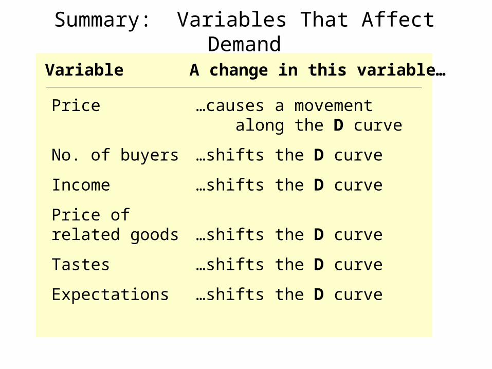
Summary: Variables That Affect Demand
Variable A change in this variable…
Price …causes a movement along the D curve
No. of buyers …shifts the D curve
Income …shifts the D curve
Price ofrelated goods …shifts the D curve
Tastes …shifts the D curve
Expectations …shifts the D curve

Summary: Variables That Affect Supply
Variable A change in this variable…
Price …causes a movement along the S curve
Input prices …shifts the S curve
Technology …shifts the S curve
No. of sellers …shifts the S curve
Expectations …shifts the S curve

AA CC TT II VV E LE L EE AA RR NN II NN G 2G 2: : Supply curveSupply curve
Draw a supply curve for tax return preparation software. What happens to it in each
of the following scenarios?
A. Retailers cut the price of the software.
B. A technological advance allows the software to be produced at lower cost.
C. Professional tax return preparers raise the price of the services they provide.
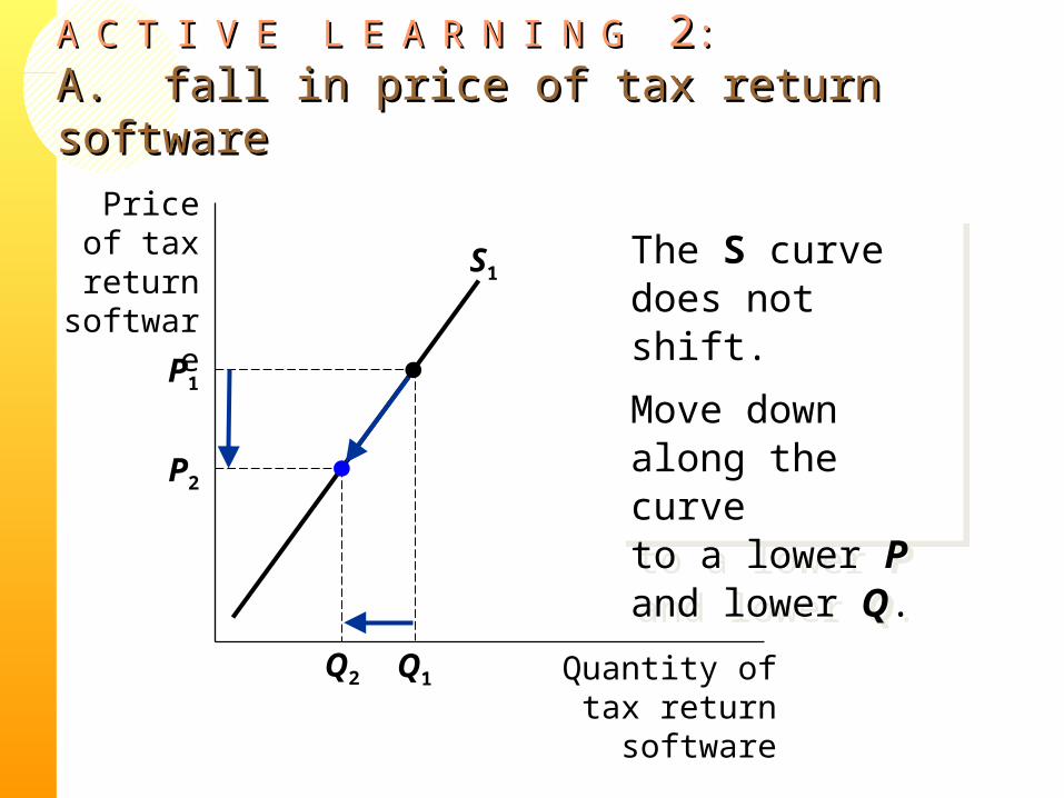
AA CC TT II VV E LE L EE AA RR NN II NN G G 22: : A. fall in price of tax return softwareA. fall in price of tax return software
The S curve does not shift.
Move down along the curve to a lower P and lower Q.
The S curve does not shift.
Move down along the curve to a lower P and lower Q.
Price of tax return software
Quantity of tax return software
S1
P1
Q1Q2
P2
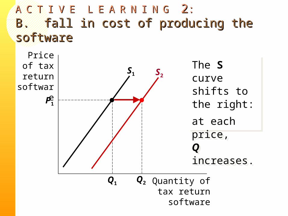
AA CC TT II VV E LE L EE AA RR NN II NN G G 22: : B. fall in cost of producing the softwareB. fall in cost of producing the software
The S curve shifts to the right:
at each price, Q increases.
The S curve shifts to the right:
at each price, Q increases.
Price of tax return software
Quantity of tax return software
S1
P1
Q1
S2
Q2
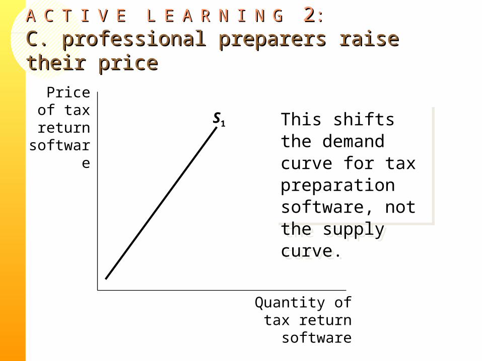
AA CC TT II VV E LE L EE AA RR NN II NN G G 22: : C. professional preparers raise their priceC. professional preparers raise their price
This shifts the demand curve for tax preparation software, not the supply curve.
This shifts the demand curve for tax preparation software, not the supply curve.
Price of tax return software
Quantity of tax return software
S1

$0.00
$1.00
$2.00
$3.00
$4.00
$5.00
$6.00
0 5 10 15 20 25 30 35
P
Q
D S
Surplus:when quantity supplied is greater than quantity demanded
Facing a surplus, sellers try to increase sales by cutting the price.
This causes QD to rise
Surplus
…which reduces the surplus.
and QS to fall…

$0.00
$1.00
$2.00
$3.00
$4.00
$5.00
$6.00
0 5 10 15 20 25 30 35
P
Q
D S
Shortage:when quantity demanded is greater than quantity supplied
Facing a shortage, sellers raise the price,
causing QD to fall
…which reduces the shortage.
and QS to rise,
Shortage

AA CC TT II VV E LE L EE AA RR NN II NN G G 33: : Changes in supply and demandChanges in supply and demand
Use the three-step method to analyze the effects of each event on the equilibrium price and quantity of music downloads.
Event A: A fall in the price of compact discs
Event B: Sellers of music downloads negotiate a reduction in the royalties they must pay for each song they sell.
Event C: Events A and B both occur.
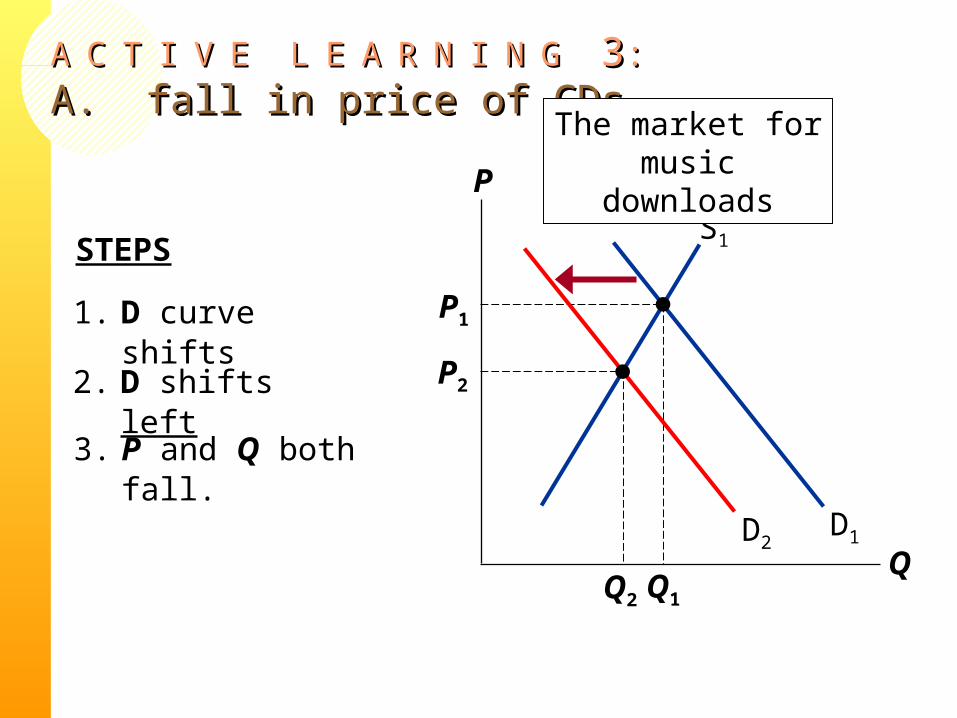
2. D shifts left
AA CC TT II VV E LE L EE AA RR NN II NN G G 33: : A. fall in price of CDsA. fall in price of CDs
P
QD1
S1
P1
Q1
D2
The market for music downloads
P2
Q2
1. D curve shifts
3. P and Q both fall.
STEPS

AA CC TT II VV E LE L EE AA RR NN II NN G G 33: : B. fall in cost of B. fall in cost of royalties royalties
P
QD1
S1
P1
Q1
S2
The market for music downloads
Q2
P2
1. S curve shifts
2. S shifts right
3. P falls, Q rises.
STEPS
(royalties are part of sellers’ costs)
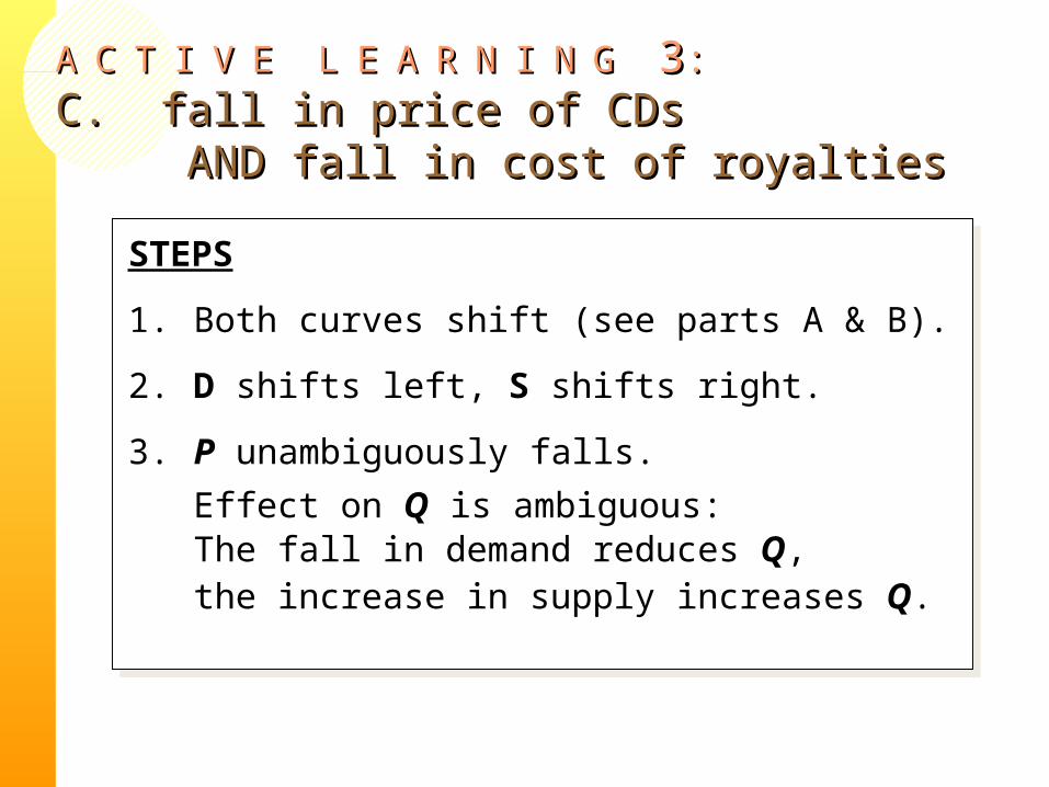
AA CC TT II VV E LE L EE AA RR NN II NN G G 33: : C. fall in price of CDs C. fall in price of CDs AND fall in cost of royalties AND fall in cost of royalties
STEPS
1. Both curves shift (see parts A & B).
2. D shifts left, S shifts right.
3. P unambiguously falls.
Effect on Q is ambiguous: The fall in demand reduces Q, the increase in supply increases Q.
STEPS
1. Both curves shift (see parts A & B).
2. D shifts left, S shifts right.
3. P unambiguously falls.
Effect on Q is ambiguous: The fall in demand reduces Q, the increase in supply increases Q.

The Determinants of Price Elasticity: A Summary
The price elasticity of demand depends on: the extent to which close substitutes are available whether the good is a necessity or a luxury how broadly or narrowly the good is defined
the time horizon: elasticity is higher in the long run than the short run.
The price elasticity of demand depends on: the extent to which close substitutes are available whether the good is a necessity or a luxury how broadly or narrowly the good is defined
the time horizon: elasticity is higher in the long run than the short run.

AA CC TT II VV E LE L EE AA RR NN II NN G G 33: : Elasticity and changes in equilibriumElasticity and changes in equilibrium
• The supply of beachfront property is inelastic. The supply of new cars is elastic.
• Suppose population growth causes demand for both goods to double (at each price, Qd doubles).
• For which product will P change the most? • For which product will Q change the most?
20

AA CC TT II VV E LE L EE AA RR NN II NN G G 33: : AnswersAnswers
21
Beachfront property (inelastic supply):
P
Q
D1 D2S
Q1
P1 A
B
Q2
P2
When supply is inelastic, an increase in demand has a bigger impact on price than on quantity.

AA CC TT II VV E LE L EE AA RR NN II NN G G 33: : AnswersAnswers
22
New cars(elastic supply):
P
Q
D1 D2
S
Q1
P1
A
Q2
P2
B
When supply is elastic, an increase in demand has a bigger impact on quantity than on price.
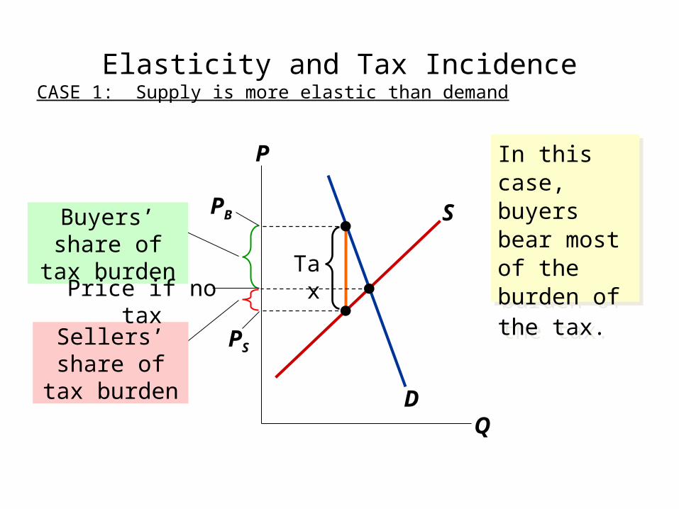
Elasticity and Tax IncidenceCASE 1: Supply is more elastic than demand
P
QD
S
Tax
Buyers’ share of tax burden
Sellers’ share of tax burden
Price if no tax
PB
PS
In this case, buyers bear most of the burden of the tax.
In this case, buyers bear most of the burden of the tax.
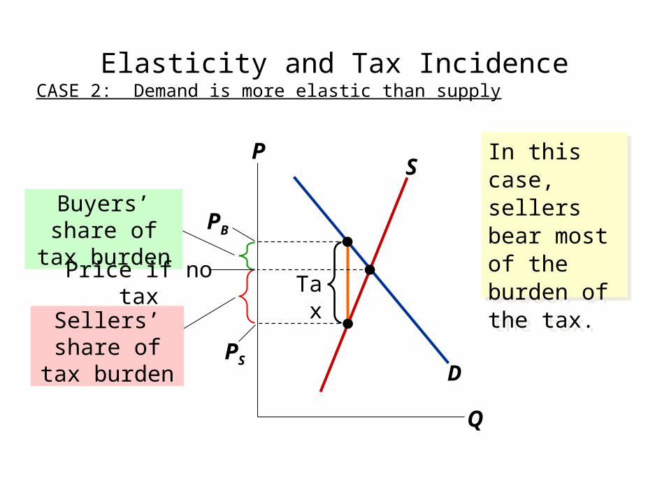
Elasticity and Tax IncidenceCASE 2: Demand is more elastic than supply
P
Q
D
S
Tax
Buyers’ share of tax burden
Sellers’ share of tax burden
Price if no tax
PB
PS
In this case, sellers bear most of the burden of the tax.
In this case, sellers bear most of the burden of the tax.

Other Elasticities• The income elasticity of demand measures the response of
Qd to a change in consumer income.
Income elasticity of demand =
Percent change in Qd
Percent change in income
Recall from chap.4: An increase in income causes an increase in demand for a normal good.
Hence, for normal goods, income elasticity > 0.
For inferior goods, income elasticity < 0.
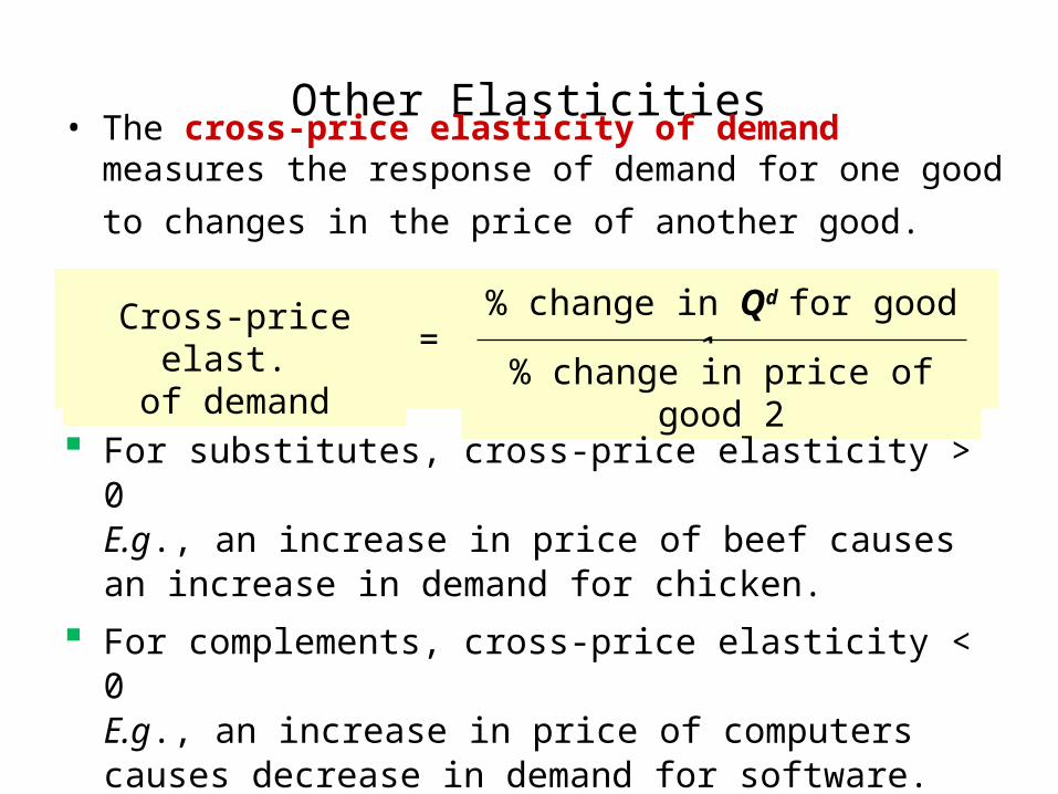
Other Elasticities• The cross-price elasticity of demand measures the response
of demand for one good to changes in the price of another
good.
Cross-price elast. of demand =
% change in Qd for good 1
% change in price of good 2
For substitutes, cross-price elasticity > 0 E.g., an increase in price of beef causes an increase in demand for chicken.
For complements, cross-price elasticity < 0 E.g., an increase in price of computers causes decrease in demand for software.

Evaluating the Market Equilibrium
Market eq’m: P = $30 Q = 15,000Total surplus = CS + PSIs the market eq’m efficient?
0
10
20
30
40
50
60
0 5 10 15 20 25 30
P
Q
S
D
CS
PS
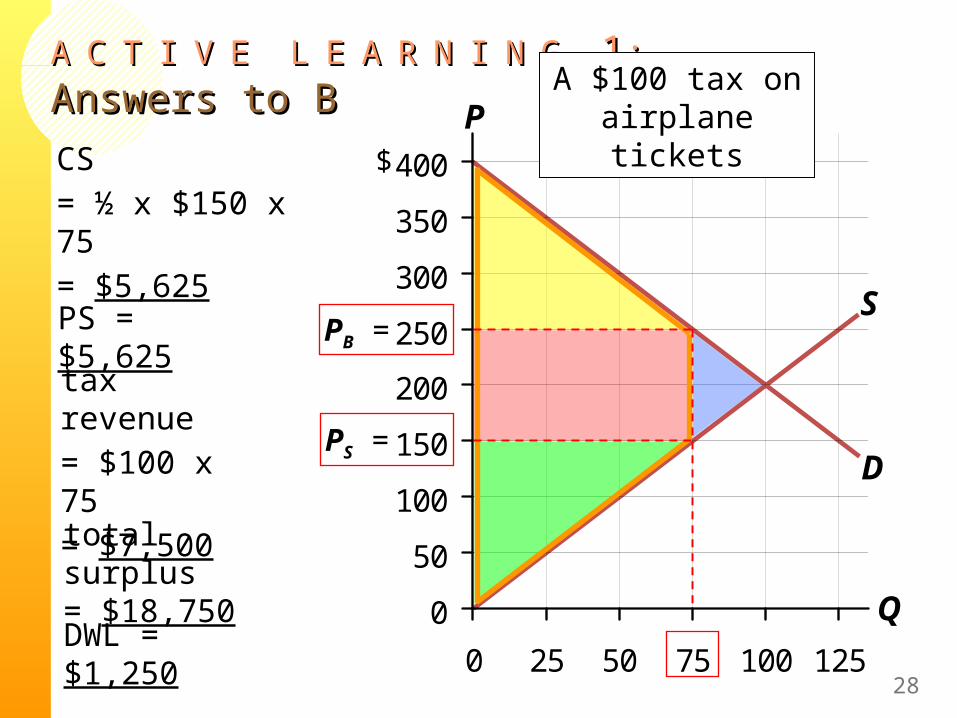
AA CC TT II VV E LE L EE AA RR NN II NN G G 11: : Answers to BAnswers to B
28
D
S
CS = ½ x $150 x 75= $5,625
0
50
100
150
200
250
300
350
400
0 25 50 75 100 125
P
Q
$
total surplus = $18,750
PS = $5,625
tax revenue= $100 x 75= $7,500
DWL = $1,250
PS =
PB =
A $100 tax on airplane tickets
$30
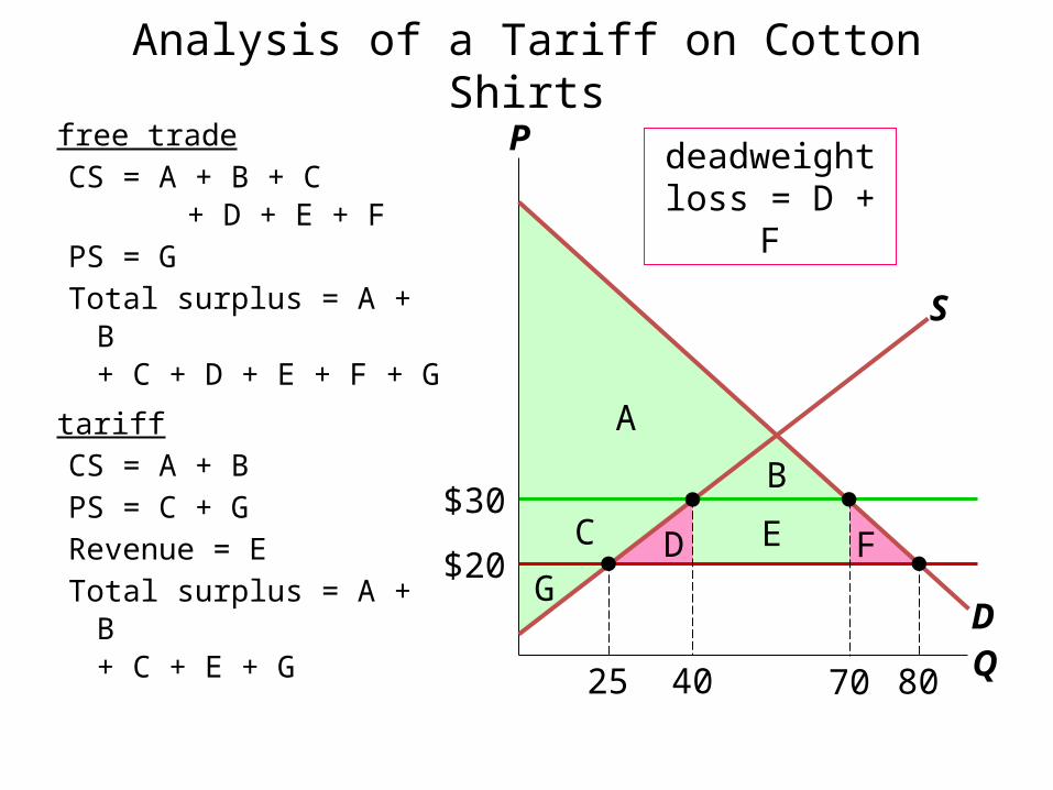
Analysis of a Tariff on Cotton Shirts
free tradeCS = A + B + C
+ D + E + FPS = GTotal surplus = A + B
+ C + D + E + F + G
tariffCS = A + BPS = C + GRevenue = ETotal surplus = A + B
+ C + E + G
P
QD
S
$20
25
Cotton shirts
40
A
B
D E
GFC
70 80
deadweight loss = D + F

AA CC TT II VV E LE L EE AA RR NN II NN G G 22: : Elasticity and DWL of a taxElasticity and DWL of a tax
Would the DWL of a tax be larger if the tax were on
A. Rice Krispies or sunscreen?
B. Hotel rooms in the short run or hotel rooms in the long run?
C. Groceries or meals at fancy restaurants?
30
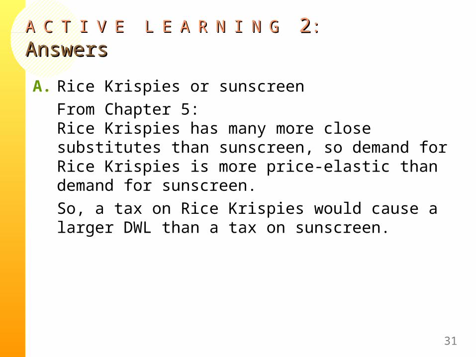
AA CC TT II VV E LE L EE AA RR NN II NN G G 22: : AnswersAnswers
A. Rice Krispies or sunscreenFrom Chapter 5: Rice Krispies has many more close substitutes than sunscreen, so demand for Rice Krispies is more price-elastic than demand for sunscreen. So, a tax on Rice Krispies would cause a larger DWL than a tax on sunscreen.
31

AA CC TT II VV E LE L EE AA RR NN II NN G G 22: : AnswersAnswers
B. Hotel rooms in the short run or long runFrom Chapter 5: The price elasticities of demand and supply for hotel rooms are larger in the long run than in the short run. So, a tax on hotel rooms would cause a larger DWL in the long run than in the short run.
32

AA CC TT II VV E LE L EE AA RR NN II NN G G 22: : AnswersAnswers
C. Groceries or meals at fancy restaurantsFrom Chapter 5: Groceries are more of a necessity and therefore less price-elastic than meals at fancy restaurants.So, a tax on restaurant meals would cause a larger DWL than a tax on groceries.
33

AA CC TT II VV E LE L EE AA RR NN II NN G G 33: : Discussion questionDiscussion question
• The government must raise tax revenue to pay for schools, police, etc. To do this, it can either tax groceries or meals at fancy restaurants.
• Which should it tax?
34
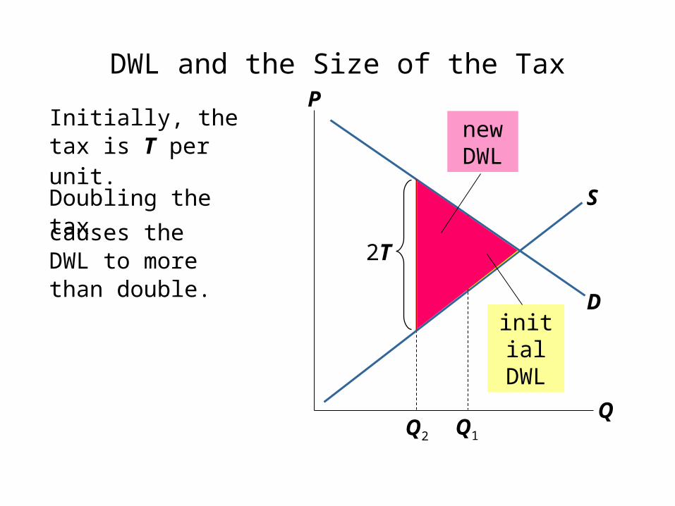
Q2 Q1
DWL and the Size of the TaxP
Q
D
S
causes the DWL to more than double.
Doubling the tax
2T T
Initially, the tax is T per unit.
initial DWL
new DWL

Q3
DWL and the Size of the TaxP
Q
D
S
Q1
3T Tcauses the DWL to more than triple.
Tripling the tax
Initially, the tax is T per unit.
initial DWL
new DWL

Q2
Revenue and the Size of the TaxP
Q
D
S
Q1
PB
PS
PB
PS
2T T
When the tax is small, increasing it causes tax revenue to rise.
Q3
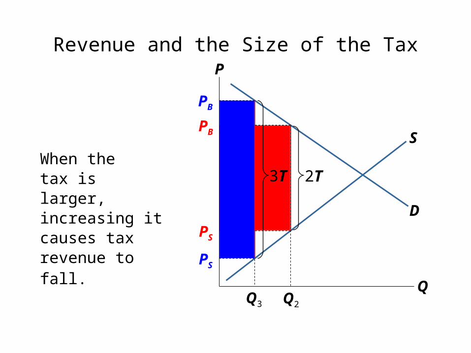
Revenue and the Size of the TaxP
Q
D
S
Q2
PB
PS
PB
PS
3T 2TWhen the tax is larger, increasing it causes tax revenue to fall.

The Laffer curve shows the relationship between the size of the tax and tax revenue.
Revenue and the Size of the Tax
Tax size
Tax revenue
The Laffer curve
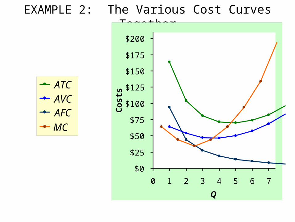
EXAMPLE 2: The Various Cost Curves Together
AFCAVCATC
MC
$0
$25
$50
$75
$100
$125
$150
$175
$200
0 1 2 3 4 5 6 7
Q
Cost
s
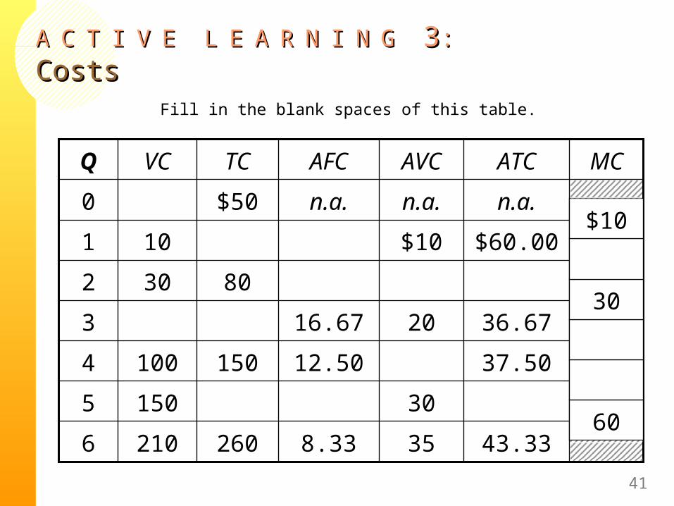
AA CC TT II VV E LE L EE AA RR NN II NN G G 33: : CostsCosts
Fill in the blank spaces of this table.
41
210
150
100
30
10
VC
43.33358.332606
305
37.5012.501504
36.672016.673
802
$60.00$101
n.a.n.a.n.a.$500
MCATCAVCAFCTCQ
60
30
$10

Use AFC = FC/QUse AVC = VC/QUse relationship between MC and TCUse ATC = TC/QFirst, deduce FC = $50 and use FC + VC = TC.
AA CC TT II VV E LE L EE AA RR NN II NN G G 33: : AnswersAnswers
42
210
150
100
60
30
10
$0
VC
43.33358.332606
40.003010.002005
37.502512.501504
36.672016.671103
40.001525.00802
$60.00$10$50.00601
n.a.n.a.n.a.$500
MCATCAVCAFCTCQ
60
50
40
30
20
$10
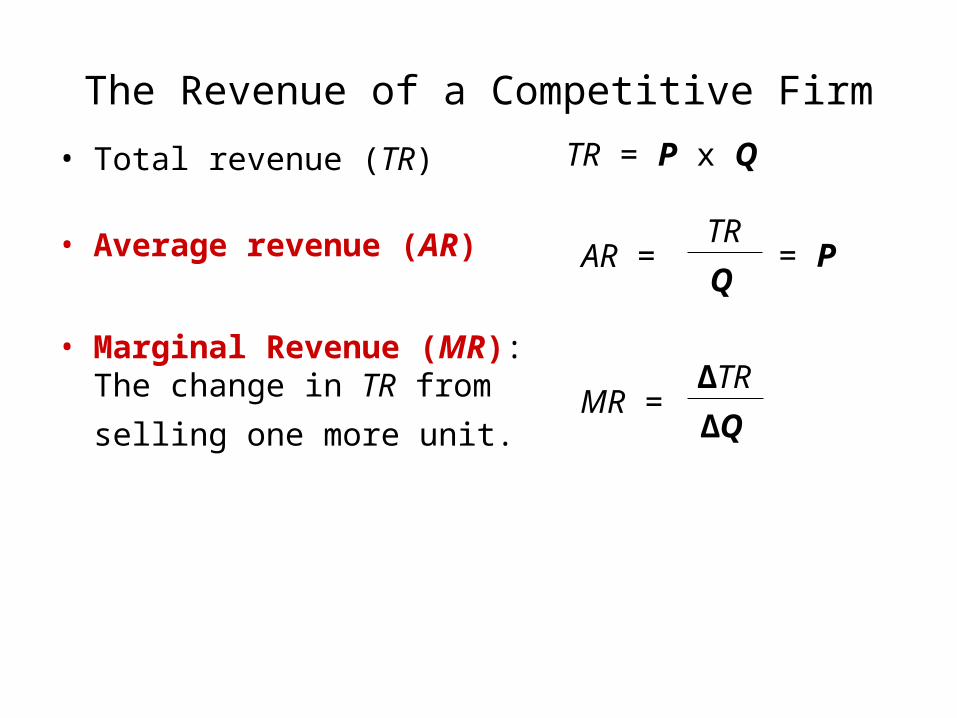
The Revenue of a Competitive Firm
• Total revenue (TR)
• Average revenue (AR)
• Marginal Revenue (MR):The change in TR from
selling one more unit. ∆TR
∆QMR =
TR = P x Q
TR
QAR = = P
© 2008 Nelson Education Ltd.
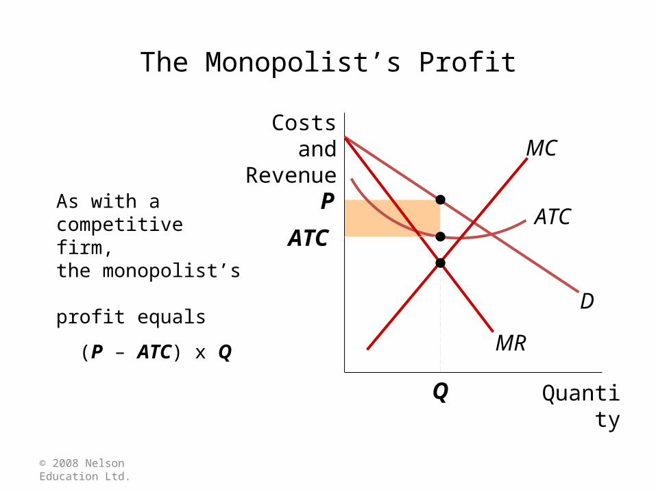
The Monopolist’s Profit
As with a competitive firm, the monopolist’s profit equals
(P – ATC) x Q
Quantity
Costs and Revenue
ATC
D
MR
MC
Q
P
ATC


