Microreg: a Traditional Tax-Benefit Microsimulation Model ... · INTERNATIONAL JOURNAL OF...

INTERNATIONAL JOURNAL OF MICROSIMULATION (2017) 10(1) 5-38

INTERNATIONAL MICROSIMULATION ASSOCIATION

Microreg: a Traditional Tax-Benefit Microsimulation Model

Extended to Indirect Taxes and In-Kind Transfers

M Luisa Maitino

IRPET (Regional Institute for Economic Planning of Tuscany) Via Pietro Dazzi 1 – 50141 Firenze (FI), Italy [email protected]

Letizia Ravagli


Nicola Sciclone


ABSTRACT: MicroReg is a tax-benefit microsimulation model, developed by IRPET (Regional

Institute for Economic Planning in Tuscany), able to simulate the main fiscal policies for all the

Italian Regions. The model is based on the EUROSTAT Survey on Income and Living Conditions

(EU-SILC). In its traditional version MicroReg can simulate direct taxes and in-cash transfers, but

recently it was extended in two directions. The first extension aims at adding indirect taxes to

simulated tax policies, thanks to a statistical matching between EU-SILC and the Italian Household

Budget Survey by Istat (National Institute of Statistics (Italy)). To improve the matching, an

estimation of the level of expenditure for each EU-SILC household is added to the variables on

which the matching is conditioned, by applying the relation between consumption and income

INTERNATIONAL JOURNAL OF MICROSIMULATION (2017) 10(1) 5-38 6

MAITINO, RAVAGLI, SCICLONE Microreg: A Traditional Tax-Benefit Microsimulation Model Extended To Indirect Taxes And In-Kind Transfers

estimated on the Bank of Italy Survey of Households Income and Wealth. The second extension

aims at including in-kind transfers, in health and education and in household disposable income.

The monetary value of in-kind transfers is estimated with the public cost of production by using

national and regional administrative data. The allocation of benefits among individuals is done by

following the so called "actual consumption approach", both for health and education. This paper

describes MicroReg, focusing on the new extensions, and the results of an application to assess the

distributive effects of fiscal policies introduced in the last few years in Italy, both on the revenue

and on the expenditure side.

KEYWORDS: MICROSIMULATION MODELS, TAX-BENEFIT SYSTEM, INDIRECT

TAXES, IN-KIND TRANSFERS

JEL classification: I3, H2, C15



1 INTRODUCTION

MicroReg is a static microsimulation model, developed by IRPET (Regional Institute for

Economic Planning in Tuscany) for the Region of Tuscany, which is able to simulate the main

fiscal policies for all the Italian Regions. Static models usually measure the short run impact of

policies, by comparing households’ income under the actual legislation and the one resulting from

reform policies. In comparing the two scenarios no changes in the structure of the population or

in the behavior of agents are contemplated. Compared to previous versions of the model (Betti et

al., (2012), Maitino & Sciclone (2008)), the one described in this paper adds two new modules to

the traditionally simulated policies (i.e. direct taxes and in-cash transfers), namely indirect taxation

and in-kind transfers (in health and education)1. MicroReg is now, therefore, able to assess the

regional impact of public policies as a whole, considering both revenues and expenditures. This

paper is structured in three sections. The first presents the model structure. The second section

describes the new modules, indirect taxes and in-kind transfers. Finally, a section concludes by

presenting an application of the extended model.

2 THE MODEL STRUCTURE

The model is divided in three phases: i) the choice of micro-data and the imputation of missing

information, namely gross income and cadastral value, ii) the calibration of sample weights, iii) the

validation of results.

2.1 The choice of micro-data and the imputation of missing information

The first phase of a microsimulation model is the choice of micro-data. In Italy many

microsimulation models use the Survey on Household Income and Wealth of Bank of Italy

(SHIW), which provides accurate information on income and household wealth2. MicroReg uses

the EUROSTAT Survey on Income and Living Conditions (EU-SILC), since it is more

representative at regional level with respect to SHIW. In this paper we describe the model built on

EU-SILC 2013 (year of income 2012). However, some important information is missing in EU-

SILC. Indeed, gross income and cadastral value of buildings need to be estimated.

2.1.1 The grossing-up procedure

The conversion of net to gross income can be done in different ways (Immervoll & O'Donoghue,



2001, Sutherland, 2001). A first solution is to estimate a coefficient of conversion from net to gross

income in a data set where both the information are available (usually for a subset of individuals).

A second solution calculates the gross income for each net income in the sample, through an

analytical inversion of all existing taxes in the year in which net income is detected. The third

solution is based on an iterative algorithm. For each individual in the sample, the procedure

estimates a gross income starting from the original net income. Fiscal rules are then applied to the

estimated gross income in order to get an estimated net income. The latter is compared with the

original one. If the two values are similar with a certain margin of error, the estimated gross income

is considered a good approximation; otherwise the procedure iteratively corrects the algorithm.

MicroReg uses the third approach and, in particular, a variant of the algorithm used for

EUROMOD, the microsimulation model for EU member states. The net income used is the sum

of several sources of taxable income for personal income tax (PIT): net individual income of

employees, net income from self-employment, net income from retirement, survivor's pension,

disability pension (excluding war pension), net income from redundancy funds, unemployment

benefits, mobility or early retirement and net income from scholarships. Incomes from land and

buildings are not included since they are considered already gross. Other incomes are excluded

because they are not taxable for PIT such as healthcare liquidations, insurance and pension arrears.

The iterative procedure is similar to the one described in Immervol and O’Donoghue (2001). At

the first iteration an arbitrarily fixed average tax rate equal to 0.22 is applied to each net income to

obtain an estimation of gross income. By applying fiscal rules to the estimated gross income an

estimated net income is obtained. Then, the estimated net income is compared with the true one.

When the difference is higher with respect to a certain margin of error the procedure continues–

by iterating–to a new estimation of gross income, by properly correcting the initial tax rate. The

procedure stops when for all sample individuals the difference between the original value and

estimated net income is less than 10 euro. When the algorithm does not converge after a certain

number of iterations, the procedure starts with a different value of the initial rate, randomly drawn

from a uniform distribution defined in the range 0-1.

2.1.2 The estimation of cadastral values

The total gross income for PIT should include incomes from land and buildings (such as rents and

cadastral values of properties). EU-SILC collects only rental income but lacks the cadastral value

of properties. The only available information is the total tax paid on buildings (IMU), without

distinction between the dwelling house and the others. Therefore, before estimating the cadastral



value we need an allocation of the total tax paid between the two components, the dwelling house

and the other buildings. Then we can apply fiscal rules to estimate cadastral values.

In MicroReg the allocation of the total property tax into the two components is made by using the

official data on the tax paid for the dwelling house registered by the Ministry of Finance (MEF). In

details, the estimation is made in the following three steps:

I) The first step in the model makes an initial split of the total tax with the following criteria:

a) If the individual is the owner of the dwelling house and does not own other buildings

then the tax is considered paid only for the dwelling house.

b) If the individual does not own neither, the dwelling house nor other buildings, the tax is

considered paid only for other buildings.

c) If the individual does not own the dwelling house but only other buildings the tax is

considered paid only for other buildings.

d) If the individual claims to own both, the dwelling house and other buildings, the tax is

initially divided in two equal parts. This is only an initial division that can change in the

second part of the procedure.

II) In the second step the tax paid for the dwelling house is estimated as follows. From the total

tax paid for dwelling houses resulting from MEF, the tax paid for dwelling houses imputed in

the first step to individuals of criteria (a) is subtracted. The resulting amount is used to bind the

tax paid for dwelling houses imputed in the first step to individuals of criteria (d). After this step

the initial division of the total tax paid of individual of criteria (d) is corrected according to real

data.

III) In the last step the tax paid for the other buildings is estimated for each individual, with the

difference between the total tax paid declared in EU-SILC and the tax paid for the dwelling

house previously estimated3.

After having obtained the two components fiscal rules can be inversely applied. Rates, as well as

deductions, are regional averages of municipal rates.

Cadastral value dwelling house =(Tax paidi,r+Tax crediti,r+Tax credit for children𝑖,𝑟)

rate_main residencei,r*1,05 *160 [1]

Cadastral value other buildings =Tax paidi,r

rate_other buildingsi,r*1,05*160 [2]

i=1,…n individuals; r=1,..K Regions



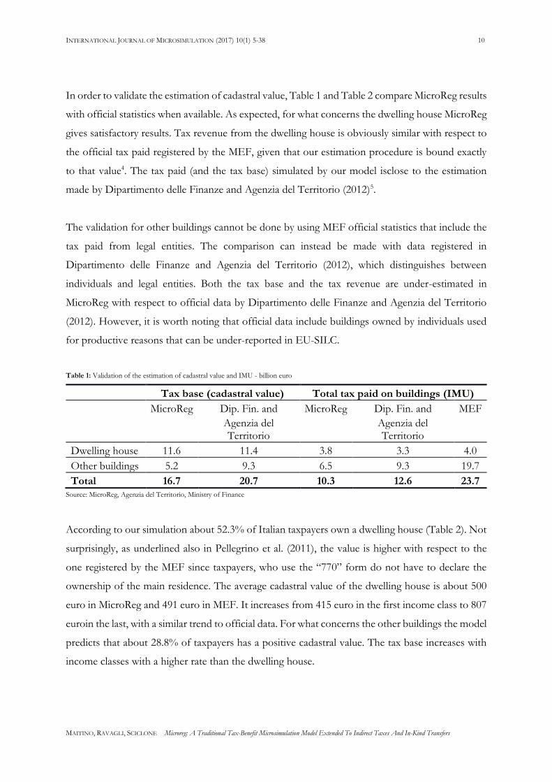
In order to validate the estimation of cadastral value, Table 1 and Table 2 compare MicroReg results

with official statistics when available. As expected, for what concerns the dwelling house MicroReg

gives satisfactory results. Tax revenue from the dwelling house is obviously similar with respect to

the official tax paid registered by the MEF, given that our estimation procedure is bound exactly

to that value4. The tax paid (and the tax base) simulated by our model isclose to the estimation

made by Dipartimento delle Finanze and Agenzia del Territorio (2012)5.

The validation for other buildings cannot be done by using MEF official statistics that include the

tax paid from legal entities. The comparison can instead be made with data registered in

Dipartimento delle Finanze and Agenzia del Territorio (2012), which distinguishes between

individuals and legal entities. Both the tax base and the tax revenue are under-estimated in

MicroReg with respect to official data by Dipartimento delle Finanze and Agenzia del Territorio

(2012). However, it is worth noting that official data include buildings owned by individuals used

for productive reasons that can be under-reported in EU-SILC.

Table 1: Validation of the estimation of cadastral value and IMU - billion euro

Tax base (cadastral value) Total tax paid on buildings (IMU)

MicroReg Dip. Fin. and

Agenzia del Territorio

MicroReg Dip. Fin. and

Agenzia del Territorio

MEF

Dwelling house 11.6 11.4 3.8 3.3 4.0

Other buildings 5.2 9.3 6.5 9.3 19.7

Total 16.7 20.7 10.3 12.6 23.7 Source: MicroReg, Agenzia del Territorio, Ministry of Finance

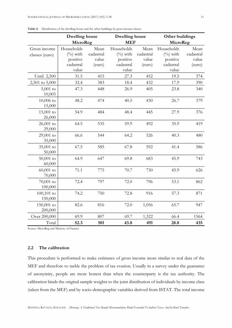
According to our simulation about 52.3% of Italian taxpayers own a dwelling house (Table 2). Not

surprisingly, as underlined also in Pellegrino et al. (2011), the value is higher with respect to the

one registered by the MEF since taxpayers, who use the “770” form do not have to declare the

ownership of the main residence. The average cadastral value of the dwelling house is about 500

euro in MicroReg and 491 euro in MEF. It increases from 415 euro in the first income class to 807

euroin the last, with a similar trend to official data. For what concerns the other buildings the model

predicts that about 28.8% of taxpayers has a positive cadastral value. The tax base increases with

income classes with a higher rate than the dwelling house.



Table 2: Distribution of the dwelling house and the other buildings by gross income classes

Dwelling house

MicroReg

Dwelling house

MEF

Other buildings

MicroReg

Gross income

classes (euro)

Households (%) with positive

cadastral value

Mean cadastral

value (euro)


cadastral value

Mean cadastral

value (euro)


cadastral value

Mean cadastral

value (euro)

Until 2,500 31.5 415 27.3 452 19.5 374

2,501 to 5,000 32.4 383 18.4 432 17.9 390

5,001 to 10,005

47.3 448 26.9 405 23.8 340

10,006 to 15,000

48.2 474 40.5 430 26.7 379

15,001 to 26,000

54.9 484 48.4 445 27.9 376

26,001 to 29,000

64.5 535 59.9 492 35.9 419

29,001 to 35,000

66.6 544 64.2 526 40.3 480

35,001 to 50,000

67.5 585 67.8 592 41.4 586

50,001 to 60,000

64.9 647 69.8 683 45.9 743

60,001 to 70,000

71.1 775 70.7 730 45.9 626

70,001 to 100,000

72.4 797 72.0 796 53.1 862

100,101 to 150,000

74.2 750 72.8 916 57.3 871

150,001 to 200,000

82.6 816 72.0 1,056 65.7 947

Over 200,000 69.9 807 69.7 1,322 66.4 1564

Total 52.3 501 43.8 491 28.8 435 Source: MicroReg and Ministry of Finance

2.2 The calibration

This procedure is performed to make estimates of gross income more similar to real data of the

MEF and therefore to tackle the problem of tax evasion. Usually in a survey under the guarantee

of anonymity, people are more honest than when the counterparty is the tax authority. The

calibration binds the original sample weights to the joint distribution of individuals by income class

(taken from the MEF) and by socio-demographic variables derived from ISTAT. The total income



considered for the calibration is the one used in the grossing up procedure, plus incomes from

buildings obtained after the estimation of cadastral values.

In literature two types of calibration methods can be found: i) independent calibration and ii)

integrative calibration. The independent calibration allows calibrating weights with households’

variables independently from individual’s variables. The convergence procedure is generally fast,

but it generates different weights for households and individuals. Integrative calibration takes into

account households’ and individuals’ variables together. It converges more slowly, but households’

and individuals’ weights are the same (as requested by the European Commission Regulation for

the SILC). In MicroReg an integrative calibration is performed with the following constraints:

taxpayers by income classes and prevailing source of income; population by age, sex, gender and

level of education; population by region of residence and by number of family members.

2.3 The validation

After having imputed missing information (see section 2.1) and calibrated sample weights (see

section 2.2) we simulate all fiscal rules that every taxpayer follows to pay PIT in the following way:

1) According to Italian fiscal rules, every taxpayer can deduct the value of the main residence6 and

other expenses (such as expenditure for disabled family members or for donations) from gross

income. Since EU-SILC does not collect detailed information about deductible expenses, we

impute their value to each taxpayer by applying a coefficient equal to the ratio between

deductions and gross income by gross income classes calculated on official data from the MEF7.

Taxable income is then simulated by subtracting deductions from gross income tax for each

taxpayer.

2) Gross PIT is simulated by applying the legal tax rates to the simulated taxable income.

3) Each taxpayer can subtract different types of tax credits from gross PIT: i) tax credits by income

source, ii) tax credits for family members and iii) other tax credits (for health expenditure,

housing works, etc.). Tax credits by income source and for family members are simulated in the

model since detailed information on income and household components are collected in EU-

SILC. The other tax credits, similar to tax deductions, are estimated by applying to each taxpayer

a coefficient given by the ratio of tax credits and gross income by gross income classes registered

by MEF8.

4) Finally, the net PIT is simulated by detracting simulated and imputed tax credits from gross



PIT. When PIT is positive, regional additional income tax is simulated by applying the different

fiscal rules of each region.

In order to validate the model, the results of our simulations are compared with data from the

MEF. Table 3 compares the distribution of the total number of taxpayers by prevailing income

source resulting from the model with respect to official statistics. The total number of taxpayers in

the model is in line with the real one and the composition is very similar to the one of the MEF.

These satisfactory results are expected given that one of the constraints of our calibration

procedure (see section 2.2) is the distribution of taxpayers by source of income and gross income

classes.

Table 3: Taxpayers by prevailing income source (millions)

MicroReg MEF Diff. (%)

Employee income 20.02 20.02 0.0

Retirement income 14.22 14.22 0.0

Self-employed income 4.60 4.60 0.0

Other sources of income 1.69 1.68 0.3

Total 40.54 40.53 0.0 Source: MicroReg and Ministry of Finance

Table 4 compares aggregate fiscal amounts simulated by the model with official data from the

MEF9. The model is able to simulate quiet gross income, taxable income, gross and net PIT well.

A little less accurate is the simulation of tax credits for family members. Results are in line with

other microsimulation models. In Ceriani et al. (2016) the model over-estimates gross income by

3% and PIT by 1%. In Pellegrino et al. (2011) the average gross income is 97.5% of the real one.

Models that also use administrative data obtain better results. In Di Nicola et al. (2015) a

microsimulation model is built on a dataset that matches EU-SILC with administrative data on PIT

and real estate datasets. Their results are very close to official statistics,except for municipal taxes,

where the difference in amounts between the model and the MEF is lower than 1%.



Table 4: Validation of the model - income year 2012 (billion euro)

MicroReg MEF Diff. (%)

Gross income 790.9 800.4 -1.2

Deductions 23.7 24.0 -1.2

Taxable income 767.2 773.6 -0.8

Gross PIT 205.1 208.2 -1.5

Tax credits by income source 41.5 41.6 -0.3

Family tax credits 11.7 11.5 2.3

Net PIT 151.3 152.3 -0.6

Regional additional income tax 11.0 11.0 -0.5 Source: MicroReg and Ministry of Finance

Figure 1 shows the density function by gross income classes simulated by MicroReg and registered

by MEF10. The overall distribution of gross income simulated by the model is close to the real one

with some specific limits. The model under-estimates the number of taxpayers under 1,000 euro

and over-estimates between 7,500 and 10,000 euro. The under-estimation in the first class depends

on a typical problem of under-reporting on small amounts of income in EU-SILC11. We do not

correct for this under-reporting problem since taxpayers under 1,000 euro represents a small part

of the total that do not pay PIT. The over-estimation of taxpayers between 7,500 and 10,000 euro

is partially offset by a small under-estimation of taxpayers between 6,000 and 7,500 euro.

Figure 1: Frequency density function for gross income - income year 2012

Note: The total number of taxpayers is 40.5 millions.

Source: MicroReg and Ministry of Finance

.0

1.0

2.0

3.0

4.0

5.0

6.0

7.0

8.0

Mil

lio

ns

of

taxp

aye

rs

MicroReg

MEF



Figure 2 reports the distribution of taxpayers with positive net PIT by gross income classes12. The

distribution of simulated PIT is quite similar with respect to official statistics. The number of

taxpayers with positive PIT is 32.3 million in MicroReg against 31.2 million in official data of the

MEF.

Figure 2: Distribution of taxpayers by gross income classes - net PIT - income year 2012

Note: The total number of taxpayers with positive net PIT is 32.3 million. Source: MicroReg and Ministry of Finance

Table 5 finally shows the main redistributive indexes calculated at the taxpayer level. The pre-tax

Gini coefficient is about 0.42. After the PIT the Gini becomes 0.38 with a decreasing of 0.05. The

strong redistribution is given by the combination of an average tax rate of 0.19 and a strong

progressive tax (Kakwani index of 0.22). As expected, the redistributive effect of regional additional

income tax is lower with respect to PIT. Indeed, several regions apply a proportional additional tax

and others impose a less progressive system of tax rates than PIT.

Table 5: Redistributive indexes

PIT Regional additional

income tax

Total

Pre-tax Gini 0.4234 0.4234 0.4234

Post-tax Gini 0.3714 0.4223 0.3692

Average tax rate 0.1913 0.0139 0.2051

Reynolds-Smolensky net redis. effect 0.052 0.0011 0.0543

Kakwani progressivity index 0.2223 0.0769 0.2125

Reranking 0.0005 0.0000 0.0006 Source: MicroReg

.0

1.0

2.0

3.0

4.0

5.0

6.0

7.0

8.0

Mil

lio

ns

of

tax

payers

MicroReg

MEF



3 EXTENSIONS OF THE MODEL

MicroReg was recently extended to indirect taxes and in-kind transfers (health and education).

Indirect taxes are estimated for all Italian Regions (multi-regional model), while in-kind transfers

are quantified only for the Region of Tuscany (for which data is available).

3.1 Indirect taxes

One of the recent developments of MicroReg is the simulation of indirect taxes after a matching

of EU-SILC with a database on consumption. An integrated database can be used with many aims:

to analyse saving and consumption behaviour; to study consumption of durable or not durable

goods; to make multidimensional analysis of poverty; and to study the impact of fiscal policies.

Despite the large availability of sample surveys, it does not exist a unique survey which collects

information both on income (y) and consumption (z) with a minimum level of accuracy and details.

Basically, given the variables x,y,z,, where x is a set of households ‘characteristics, the database lacks

completely or partially, the joint observation of all three. The only way to integrate the two datasets

is to assume that information in x is sufficient to jointly determine both y and z. Literature suggests

many solutions to integrate the two datasets (Decoster et al., 2007). Basically, at least two

approaches can be distinguished and they are explained in the following.

One, the so called explicit approach, uses Engel curves to impute expenditure to the income database.

According to this approach a regression of each expenditure share variables common to the

consumption and the income database (usually disposable income and socio-demographic

characteristics) is estimated on the consumption database. Then, the estimated coefficients are

applied to records in the income database to impute expenditure shares for each good. An

application of this procedure in Italy is in O’Donoghue et al. (2004). The survey which collects

information on income is the SHIW, while the consumption database is the Italian Household

Budget Survey (HBS). In the latter a variable on disposable income is collected (even if

underestimated), so a regression of total consumption on income and socio-demographic

characteristics is estimated. The estimated coefficients are then applied to SHIW to impute total

consumption. Budget shares of total consumption are subsequently estimated in HBS trough Engel

curves and applied to the imputed total consumption in SHIW. The explicit approach is more

recently applied in Taddei (2012), where the income database is EU-SILC and the consumption

one is HBS. The procedure is made in two steps. Taddei (2012) first applies a statistical matching



to impute income from EU-SILC to HBS. Once imputed income to HBS by following the explicit

approach, it estimates Engel curves to associate to each observation in EU-SILC a vector of budget

shares for each consumption good.

The second approach, called implicit approach, tries to find for each household of the income

database the most similar in the consumption database. This approach is not based on a statistical

model or on theoretical assumptions that explain consumption behaviour, but on a statistical

matching (D’Orazio et al., 2002). The matching links similar units through a distance function that

should be minimized. Units are compared according to a set of socio-demographic characteristics,

common to the two databases. The matching can be done only if the two surveys are random

samples extracted from the same population. In Italy a statistical matching between the Bank of

Italy Survey of Households Income and Wealth and HBS is in Battellini et al. (2009), in which the

integrated database is mainly used to compile Social Accounting Matrices (SAM). More recently,

in Pisani and Tedeschi (2014) a matching technique is applied to build an integrated dataset useful

for direct and indirect tax benefit microsimulation models13. The income database is the Bank of

Italy Survey of Households Income and Wealth and the consumption one is HBS. Before doing

the matching, Pisani and Tedeschi (2014) estimate a propensity score to synthesize in one scalar all

the different variables common to the two databases. The propensity score is indeed the estimated

probability to belong to SHIW conditioning on the common set of characteristics. Then, they apply

two different matching procedures. In the first one they associate to each observation in SHIW the

one in HBS with the closest propensity score (nearest neighbour within calliper). In the second

they use a function (called Mahalanobis) to measure for each unit in SHIW the distance to all units

in HBS in the common variables (included the propensity score). The unit in HBS with the lower

distance is then associated to each unit in SHIW. According to Pisani and Tedeschi (2014) the

Mahalanobis distance function performs better than the nearest neighbour method.

In MicroReg an implicit approach based on a matching between EU-SILC and HBS is

implemented. Therefore, our method is not parametric as the ones used in O’Donoghue et al.

(2004) and Taddei (2012), but it is more similar to Pisani and Tedeschi (2014). The objective of the

matching is to link each family in EU-SILC to the most similar in HBS, given the set of common

observable variables. The matching is shown in detail in the following three steps:

I) Preliminarily a comparison between the common variables is made by using a T-test for

the mean difference and a 𝜒2test for equality of distribution (results are reported in

appendix, tables A.4 and A.5). After, variables are standardized with the same classifications



and encodings and aggregated at household level.

II) Secondly, we select the conditioning variables for the matching. We do not estimate a

propensity score, as in Pisani and Tedeschi (2014), but we select among the distinct

common variables. The common set of variables is selected by making a regression of

consumption on socio-demographic characteristics (see results for the Centre of Italy in

appendix, table A.6). Some variables refer to households characteristics (such as residence

area, number of components, number of rooms, presence of loan to pay, personal

computer and dishwasher ownership, access to internet). Other variables refer to socio-

demographic characteristics of household components (number of children, number of

adults, type of work, number of earners).

In order to improve the matching, for each EU-SILC household an estimation of total

consumption is added to the set of common variables. More precisely, a regression of total

consumption on household income is estimated for income quintiles in the Bank of Italy

Survey of Households Income and Wealth. Indeed, SHIW collects detailed information on

income, but also an aggregate measure of consumption. Then, estimated coefficients are

applied to EU-SILC households to find the imputed total consumption that can be used in

the matching.

III) Similarly to Pisani and Tedeschi (2014) we define a proximity function to integrate

household by household information collected from both surveys. Our matching is made

in two steps. A first exact matching for a selection of common variables (geographical area

and number of components) is implemented. The exact matching allows linking each EU-

SILC household with the corresponding HBS household, given the two selected variables.

For the other variables the following proximity function is defined:

𝑠(𝑥, 𝑦) = max ∑ ∑ 𝑠𝑖(𝑥ij, 𝑦ij)∀𝑗 ∈ 𝑁𝑃𝑖=1

𝑁𝑗=1 [3]

otherwise 0

x if 1),(

ij

ij

ijiji

yyxs [4]

Basically, the distance function counts for every household in EU-SILC, the number of variables

with the same value in EU-SILC and in HBS. The total consumption is considered equal if the

difference is lower than 1,000 euro. Finally, for each EU-SILC household the HBS household with

the higher number of variables with the same value is associated. When two HBS household have

the same number of equal variables the household with the lower difference of total consumption



is linked.

In the integrated database the Value Added Tax (VAT) rates by type of expenditure are inversely

applied to find the production price (HBS collect retails prices which include indirect taxes). Given

the tax base VAT can subsequently be simulated.

The following statistics are used to validate the matching procedure and the VAT simulation. In

line with expectations, the food share is higher in the South of Italy than in the North-Centre

(Table 6) and the propensity to consume decreases by income deciles (Table 7).

Table 6: Food share by geographical area

Area Expenditure (euro) Income (euro) Food share

North West 487.5 2,454.80 0.1986

North East 446.1 2,450.70 0.182

Centre 504.3 2,356.50 0.214

South 506.7 1,893.80 0.2675

Italy 488.7 2,259.20 0.2163 Source: MicroReg

Table 7: Propensity to consume by income deciles

Decile Italy

0 1.26

1 1.07

2 0.96

3 0.93

4 0.87

5 0.83

6 0.78

7 0.76

8 0.69

9 0.56

Total 0.92 Source: MicroReg

The total VAT base is about 419 billion euro while tax revenue is 58 billion14 (Table 8). The

validation of the simulation of VAT is not an easy task, as Taddei (2012) underlines, since official

statistics about the revenue deriving from households are not available. As expected, our simulated

tax revenue is lower with respect to the official data estimated by ISTAT (2016)15 (about 94 billion



euro). Indeed, the official data includes the tax paid from public administration, no-profit

institutions and others that, on the contrary, is not included in our simulation on final consumption

of households. According to Taddei (2012) the percentage of total revenue that derives from

households is about 70%. D’Agosto et al. (2012) estimates that about 68% of the potential tax

revenue depends on final consumption of households. By applying these percentages to the total

tax paid estimated by ISTAT (2016) a value around 64-66 billion is obtained, not very far from our

result (58 billion euro). Further, our simulated tax revenue is in the middle between the one

obtained by Taddei (2012), about 72 billion euro, and the one simulated by Gastaldi et al. (2014),

around 49 billion euro.

Table 8: VAT tax base and revenue (billion euro)

VAT rate Tax base

Tax revenue

4% 77.9 3.1

10% 166.8 16.7

22% 174.2 38.3

Total 418.8 58.1 Source: MicroReg

Finally, Table 9 shows redistributive indexes, calculated at household level, for each VAT rate. Not

surprisingly, VAT has a negative redistribution role. Indeed, the Gini of disposable income

increases after the tax. Among the different rates, it is easily to see that the reduced rate (4%) has

the most regressive impact with a negative Kakwani of 0.21. The reduced rate is applied to those

essential goods that each household needs and, consequently, the fiscal burden is higher for lower

incomes. Despite this, the ordinary rate shows the strongest negative redistributive effect owing to

the highest average tax rate.

Table 9: Redistributive indexes

VAT rate 4% 10% 22% Total

Pre-tax Gini 0.3009 0.3009 0.3009 0.3009

Post-tax Gini 0.3017 0.3040 0.3059 0.3102

Average Tax Rate 0.0039 0.0208 0.0470 0.0717

Reynolds-Smolensky net redis. effect -0.0008 -0.0031 -0.0050 -0.0093

Kakwani progressivity index -0.2116 -0.1426 -0.0931 -0.1139

Re-ranking 0.0000 0.0001 0.0004 0.0005 Source: MicroReg



In conclusion, the matching results and the simulation of VAT are satisfactory and in line with

expectations. The indirect tax module of MicroReg can then be used to simulate different scenarios

of VAT reforms.

3.2 In-kind transfers

The second extension of MicroReg concerns in-kind transfers16. Many empirical studies about

inequality and poverty do not consider benefits from public expenditure in in-kind transfers like

education, health, transport and so on. The monetary disposable income is, however, only a part

of the household welfare, which depends also on the public subsidies for the production and the

financing of services. The inclusion of in-kind transfers in a microsimulation model allows: i) to

compare their distributive impact with respect to in-cash transfers, ii) to make a more correct

comparison between countries which have a different composition of in-cash and in-kind transfers,

iii) to monitor the effects of cuts in services and spending reviews.

In order to estimate the distributive effects of in-kind transfers many methodological issues should

be addressed (Gigliarano & D’Ambrosio, 2009). The first issue refers to the imputation of a

monetary value to in-kind transfers. Usually the monetary value is quantified by estimating the

average production cost of the public sector, even if this approach has several limits. For example,

it does not take into account that differences in production costs could depend on differences in

the quality of services, in inefficiency or on different costs of inputs.

Once quantified the monetary value, in-kind transfers should be imputed to the

individuals/households of the sample (in our case EU-SILC). In literature, two approaches have

been used, the actual consumption approach (AA) and the insurance value approach (IA).

The AA imputes the monetary value of in-kind transfers only to individuals who actually use the

service. The advantage of this approach is that it considers the true usage of services and it takes

into account individuals’ differences. Disadvantages are many. First, the attribution is not

independent on the time interval considered, during which the use of services could be entirely

random. Second, it does not consider different needs of families. For example, it can impute a large

monetary value to old people who need many health services with a consequent strong re-ranking

(old people become richer than people with more income who do not use services).



The IA imputes to every individual an average monetary value of in-kind transfers by demographic

characteristics (usually age and gender), without taking into account the actual use of services. In

health, for example, a sort of insurance premium against diseases is imputed to all individuals by

demographic characteristics. According to the IA, the use of health services should not depend on

random reasons (as in the AA), but on demographic differences. Also this approach, however, has

some disadvantages. The possibility to have a re-ranking is still present (even if less likely than in

the AA) and it does not take into account individuals’ differences.

In literature the AA is often applied for education. In health the debate is more open. In studies

that compare both the approaches, it has been noticed a higher distributive impact of IA than AA

(Baldini et al., 2007).

In evaluating the distributive impact of in-kind transfers further methodological issues must be

addressed. Usually the long run effects of in kind-transfers (like education returns) are not

considered in empirical studies. Further, there is no consensus about the correct counterfactual

(the starting income) that should be used to evaluate the distributive effect of in-kind transfers and

about the equivalence scale that should be used. Moreover, studies about in-kind transfers typically

neglect externalities. In other words, by imputing the benefit only to students or to patients they

under-estimate the positive externalities of education and health on the entire population.

In MicroReg the monetary value of in-kind transfers is quantified with the cost of production of

the public sector. The monetary value is imputed to individuals through the AA approach, both

for education and for health. The equivalence scale is not used for in-kind transfers, but a per-

household member in-kind value is attributed to each individual. The modified OECD scale is

used only for the monetary disposable income. In what follows methodological choices and data

used for education and health are described in details. The simulation of in-kind transfers is

performed only for the Region of Tuscany, both for education and health17.

3.2.1 From pre-school to secondary education

To quantify the cost of production of pre-school, primary school, middle school and high school

data from the balance sheet of the national government are used. Indeed, the biggest part of public

expenditure derives from the central level. So, the total expenditure for each level of education is

taken from balance sheets. Then, the regional expenditure is estimated by applying the distribution

of teachers by Region to the national expenditure. The per-student value of education is afterwards



estimated by dividing the total regional expenditure by the number of students (taken from the

Ministry of Education) for each level of education. Finally, the per-student value is imputed to

students by exploiting the information about the school attended, collected in EU-SILC, and about

the age of children.

3.2.2 Higher education

In order to find the monetary value of higher education, first the cost of production is calculated

and second taxes paid by each student are simulated. To quantify the cost of production the balance

sheets of the three Tuscan universities (Florence, Pisa and Siena)18 are used. The per-student value

is obtained by dividing the total cost of production by the number of students (taken from the

Ministry of Education). University taxes are composed of three parts: entry fee, fee for the right to

study and contributions. The first two are a fixed amount; the third depends on a mean test

instrument called ISEE (Equivalent Economic Situation Indicator). ISEE and taxes are simulated

in the model for each student. The net benefit from tertiary education is given by the difference

between the per-student cost of production and simulated taxes. The net per-student value is

imputed to students by exploiting the information collected in EU-SILC.

3.2.3 Health services

For health in-kind transfers administrative data from the Region of Tuscany (year 2010) are

exploited. Administrative data collects both the numbers of users and the costs of production for

each health service that is hospital services (cards hospital discharges), outpatient services,

pharmaceutical services and rehabilitation services19. To attribute health consumption to

individuals we applied the Monte Carlo method. First, a probability to consume a certain service is

estimated for intersections (cells) of socio-demographic characteristics (gender, citizenship, age

classes and level of education). Second, the service is attributed to individuals by comparing the

estimated probability with a random number from a uniform distribution in the interval 0-1. For

the selected individuals the in-kind benefit of each service (evaluated by its cost of production) is

imputed.

3.2.4 The distributive impact of in-kind transfers

The incidence of simulated in-kind transfers on income by quintiles of equivalent disposable

income shows the important distributive role of public expenditure, both in education and health

(Figures 3 and 4).



Figure 3: Incidence of education transfers on disposable income by equivalent household disposable income quintile - Tuscany

Source: MicroReg

In education, the incidence clearly decreases with income and it is particularly high in the first

quintile for high and middle school. The incidence is lower for pre-school even if still decreasing

with income (Figure 3). Also health expenditure seems to affect more low income quintiles. Among

the different services considered hospital ones tend to have a stronger impact (Figure 4).

Figure 4: Incidence of health transfers on disposable income by equivalent household disposable income quintile - Tuscany

Source: MicroReg

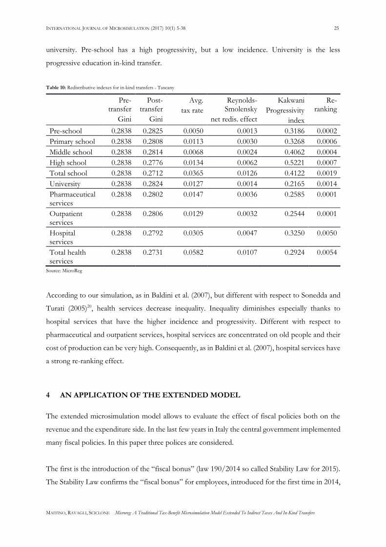
These descriptive results are confirmed by the redistributive indexes (Table 10) calculated at the

individual level. All in-kind transfers in education have a positive redistributive impact like in

Baldini et al. (2007). Further, similarly to Baldini et al. (2007) the stronger redistribution derives

from primary, middle and high school. The progressivity index is particularly elevated for middle

and high school. The reduction in the post-transfer Gini index is lower for pre-school and

.0

5.0

10.0

15.0

20.0

25.0

1° quintile 2° quintile 3° quintile 4° quintile 5° quintile

%

University

High school

Middle school

Primary school

Pre-school

.0

5.0

10.0

15.0

20.0

1 2 3 4 5

%

Pharmaceutical services Outpatient services Hospital services



university. Pre-school has a high progressivity, but a low incidence. University is the less

progressive education in-kind transfer.

Table 10: Redistributive indexes for in-kind transfers - Tuscany

Pre-transfer

Gini

Post- transfer

Gini

Avg.

tax rate

Reynolds-Smolensky

net redis. effect

Kakwani

Progressivity

index

Re-ranking

Pre-school 0.2838 0.2825 0.0050 0.0013 0.3186 0.0002

Primary school 0.2838 0.2808 0.0113 0.0030 0.3268 0.0006

Middle school 0.2838 0.2814 0.0068 0.0024 0.4062 0.0004

High school 0.2838 0.2776 0.0134 0.0062 0.5221 0.0007

Total school 0.2838 0.2712 0.0365 0.0126 0.4122 0.0019

University 0.2838 0.2824 0.0127 0.0014 0.2165 0.0014

Pharmaceutical services

0.2838 0.2802 0.0147 0.0036 0.2585 0.0001

Outpatient services

0.2838 0.2806 0.0129 0.0032 0.2544 0.0001

Hospital services

0.2838 0.2792 0.0305 0.0047 0.3250 0.0050

Total health services

0.2838 0.2731 0.0582 0.0107 0.2924 0.0054

Source: MicroReg

According to our simulation, as in Baldini et al. (2007), but different with respect to Sonedda and

Turati (2005)20, health services decrease inequality. Inequality diminishes especially thanks to

hospital services that have the higher incidence and progressivity. Different with respect to

pharmaceutical and outpatient services, hospital services are concentrated on old people and their

cost of production can be very high. Consequently, as in Baldini et al. (2007), hospital services have

a strong re-ranking effect.

4 AN APPLICATION OF THE EXTENDED MODEL

The extended microsimulation model allows to evaluate the effect of fiscal policies both on the

revenue and the expenditure side. In the last few years in Italy the central government implemented

many fiscal policies. In this paper three polices are considered.

The first is the introduction of the “fiscal bonus” (law 190/2014 so called Stability Law for 2015).

The Stability Law confirms the “fiscal bonus” for employees, introduced for the first time in 2014,



with effects from 2015 onwards. The government expects from the “fiscal bonus” indirect positive

effects on consumption. More precisely, the “fiscal bonus” is a fixed amount of 960 euro per year

(80 euro per month) for employees with gross income under 24,000 euro and it is decreasing for

employees with gross income between 24,000 and 26,000 euro, as explained in the following table

(Table 11). The bonus is attributed to employees with a gross PIT higher than tax credit for

employees.

Table 11: Fiscal bonus scheme

Income (euro) Fiscal bonus (euro)

Under 24,000 960

Between 24,000 and 26,000 960*[1-(income-24,000)/(26,000-24,000)]

Over 26,000 0 Source: Stability Law for 2015

The second policy is the safeguard clause about the increase of VAT (law 190/2014 so called

Stability Law for 2015). In Italy three VAT rates are applied: the ordinary rate is now 22%, the

decreased rate is 10% and concerns tourist services and some types of food, and the minimum rate

is 4% for basic necessities. The law 190/2014 states that VAT rates will increase from 10% to 12%

and from 22% to 24% in 2016 if other resources to meet budget constraints will not be found

(safeguard clause). In the following years further increases are established (see Table 12).

Table 12: VAT rates: safeguard clause

Year Ordinary rate Decreased rate

2015 22% 10%

2016 24% 12%

2017 25% 13%

2018 25.5% 13% Source: Stability Law for 2015

The third policy is the variation in health and education expenditure between 2013 and 2016 as

expected by the estimated budget of the State and by the Economic and Financial Document

(DEF) 2015. In the last few years the central government decided for many cuts and spending

review operations (Table 13). Between 2013 and 2016 there will be a decrease in education public

spending and an increase in health (current prices). These variations (in percentage) are applied to

the monetary value of in-kind transfer estimated in MicroReg to evaluate the redistributive effects.



Table 13: Education and health expenditure (million euro) – Italy

Year School University Health

2013 41,899 6,997 110,044

2016 41,028 6,931 113,372 Source: DEF 2015 and budget of the State

In order to evaluate the total distributive effects of the three policies we compare the disposable

income in 2013 (without the fiscal bonus and the increase in VAT and with the 2013 value of in-

kind transfers) and the disposable income in 2016 (with the fiscal bonus, the increase in VAT and

with the 2016 value of in-kind transfers) (Figure 5).

Figure 5: Variation of household disposable income and its components by equivalent disposable income quintiles - Tuscany

Source: MicroReg

The fiscal bonus has a strong effect and it is more favourable to central quintiles. It costs about

656 million of euro and it includes 788 thousands of beneficiaries in Tuscany (about 21% of the

total population that lives in the 38% of the total number of households).

The increase in VAT rates has a clear regressive impact, since the disposable income is reduced

more for the first quintile with respect to the others. Similar results are in Arachi et al. (2012). By

simulating an increase to 23.5% and to 12.5% in the ordinary and the reduced tax rate they observe

a regressive redistribution.

Cuts in school expenditure have a clear regressive impact since the decrease in disposable income

is decreasing by quintile of income. The effect of reduction in university expenditure is negligible.

The increase in disposable income due to the raise in health expenditure is higher for the first

-2%

-2%

-1%

-1%

0%

1%

1%

2%

2%

3%

1 2 3 4 5

Health

University

School

Fiscal bonus

VAT

Total



quintiles of income. By considering all the three policies together the effect is positive for central

quintiles, with a variation in disposable income of about 0.8% (thanks especially to the fiscal bonus).

For the first and the last quintile, the increase in disposable income is lower. Therefore, if the

increase in VAT rates will not be avoided the positive effect of the fiscal bonus on consumption

expected by the national government (most from the first quintile) could miss.

Table 14: Redistributive indexes - Tuscany

Gini Theil

Original disposable income 0.2836 0.1450

Disposable income with VAT increase 0.2851 0.1470

Disposable income with fiscal bonus 0.2815 0.1426

Disposable income with variation in school expenditure 0.2838 0.1451

Disposable income with variation in university expenditure 0.2836 0.1450

Disposable income with variation in health expenditure 0.2834 0.1447

Final disposable income 0.2829 0.1445 Source: MicroReg

Inequality indexes, calculated at household level, confirm these results (Table 14). After the increase

in VAT the Gini increases. On the contrary, it decreases with the introduction of fiscal bonus. In-

kind transfers have positive effect in inequality. When their value decreases (school and university)

the Gini increases, the opposite when their value increases (health).

REFERENCES

Arachi, G., Bucci, V., Longobardi, E., Panteghini, P.M., Parisi M., L., Pellegrino, S., & Zanardi, A. (2012).

Fiscal Reforms during Fiscal Consolidation: The Case of Italy, FinanzArchiv: Public Finance Analysis, 68(4),

445-465.

Baldini, M., Bosi, P., & Pacifico, D. (2007). Gli effetti distributivi dei trasferimenti in-kind: il caso dei servizi

educativi e sanitari, in Brandolini A. and Saraceno C. (a cura di), Povertà e benessere. Una geografia delle

disuguaglianze in Italia, Bologna: Il Mulino, 411-422.

Battellini, F., Coli, A., & Tartamella, F. (2009). La SAM come strumento di integrazione e analisi, Rivista di

statistica ufficiale, 2-3:35-62.

Betti, G., Maitino, M., & Sciclone, N. (2012). A che cosa servono i modelli di microsimulazione? Tre

applicazioni usando microReg, Scienze Regionali, 2(2), 101-119.



Bianchini, L., Maitino, M., Piazza, S., Ravagli, L., & Sciclone, N. (2013). Federalismo fiscale e redistribuzione:

l’effetto distributivo dei benefici in-kind a livello regionale. Un’applicazione a due Regioni italiane, IRPET.

Ceriani, L., Figari, F., & Fiorio, C. (2016). ITALY (IT) 2013-2016 Euromod version G4.0.

Decoster, A., De Rock, B., De Swerdt, K., Loughrey, J., O’Donoghue, C., & Verwerft D. (2007). Comparative

Analysis of Different Techniques to Impute Expenditures into an Income Data Set, Project no: 028412, AIM-AP

Accurate Income Measurement for the Assessment of Public Policies.

Di Nicola, F., Mongelli, G., & Pellegrino, S. (2015). The static microsimulation model of the Italian

Department of Finance: Structure and first results regarding income and housing taxation. Economia pubblica.

Dipartimento delle Finanze and Agenzia del Territorio (2012). Gli immobili in Italia 2012 - Ricchezza, reddito e

fiscalità immobiliare.

D’Agosto, E., Marigliani, M., & Pisani, S. (2012). Asimmetrie territoriali nel gap IVA, Atti della Conferenza

XXIV SIEP “Economia informale, evasione fiscale e corruzione”, Università di Pavia, SIEP.

D’Orazio, M., Di Zio, M., & Scanu, M. (2002). Statistical Matching and Official Statistics, Rivista di statistica

ufficiale, 1, 5-24.

Gastaldi, F., Liberati, P., Pisano, E., & Tedeschi, S. (2014). Progressivity-improving VAT reforms in Italy, University

of Pavia, SIEP, wp, 672.

Gigliarano, C., & D'Ambrosio, C. (2009). Public health transfers in kind: measuring the distributional effects in Italy,

Università Commerciale Luigi Bocconi, Econpubblica Centre for Research on the Public Sector, Working

Paper, (145).

Immervoll, H., & O'Donoghue, C. (2001). Imputation of gross amounts from net incomes in household surveys: an

application using EUROMOD, EUROMOD Working Paper EM1/01.

Istituto Nazionale di Statistica (2016). Sintesi dei conti ed aggregati economici delle Amministrazioni pubbliche, 2016.

Maitino, M. L., & Sciclone, N. (2008). Il modello di microsimulazione fiscale dell’IRPET Microreg, IRPET 5/08-

ebook.

O’Donoghue, C., Baldini, M., & Montovani, D. (2004). Modelling the Redistributive Impact of Indirect Taxes in

Europe: An Application of Eurmod, EUROMOD Working Paper no. EM7/01.

Pellegrino, S., Piacenza, M., & Turati, G. (2011). Developing a static microsimulation model for the analysis

of housing taxation in Italy, International Journal of Microsimulation, 4(2), 73-85.



Pisani, E., & Tedeschi, S. (2014). Micro Data Fusion of Italian Expenditures and Incomes Surveys, WP n.164,

Working Papers Series of the Department of Public Economics - Sapienza University of Rome.

Sonedda, D., & Turati, G. (2005). Winners and losers in the Italian Welfare State: A microsimulation analysis

of income redistribution considering in-kind transfers, Giornale degli Economisti, 64(4), 423-464.

Sutherland, H. (2001). Final report EUROMOD: An Integrated European Benefit Tax Model, Working Paper, n.

EM9.

Taddei, A. (2012). The tax shift from labor to consumption in Italy: a fiscal microsimulation analysis using EUROMOD,

WP 9/2012, University of Genoa.



APPENDIX

Table A.1: Validation of the model - income year 2012 (billion euro)

Gross income Deductions Taxable income

Gross PIT

Micro

Reg

MEF Micro

Reg

MEF Micro

Reg

MEF Micro

Reg

MEF

Piedmont 67.5 66.8 2.0 2.1 65.5 64.4 17.5 17.3

Aosta valley 2.1 2.1 0.1 0.1 2.1 2.0 0.6 0.5

Lombardy 164.5 163.6 5.0 5.1 159.5 157.6 44.0 44.0

Liguria 23.8 25.1 0.7 0.8 23.1 24.2 6.3 6.5

Trento 8.4 8.3 0.3 0.3 8.2 8.0 2.2 2.1

Bolzano 8.5 8.8 0.3 0.3 8.2 8.5 2.2 2.3

Veneto 69.9 71.8 2.0 2.6 67.9 69.0 18.1 18.5

Friuli Venezia Giulia

18.2 19.0 0.5 0.6 17.7 18.4 4.6 4.9

Emilia Romagna 71.4 70.9 2.1 2.5 69.3 68.0 18.6 18.4

Tuscany 54.1 54.4 1.6 1.8 52.5 52.3 13.8 14.0

Umbria 11.6 11.8 0.3 0.4 11.3 11.4 2.9 3.0

Marche 19.7 20.6 0.6 0.8 19.1 19.8 5.0 5.2

Lazio 84.3 83.2 2.6 1.9 81.6 80.7 22.5 22.6

Abruzzo 14.2 15.3 0.4 0.4 13.8 14.9 3.5 3.9

Molise 3.1 3.3 0.1 0.1 3.0 3.2 0.8 0.8

Campania 49.3 50.5 1.5 1.1 47.8 49.3 12.6 12.9

Apulia 38.2 39.0 1.1 1.0 37.0 38.1 9.3 9.8

Basilicata 5.1 5.7 0.2 0.2 4.9 5.5 1.3 1.4

Calabria 18.4 17.0 0.6 0.4 17.8 16.7 4.6 4.2

Sicily 39.4 45.0 1.2 1.0 38.2 44.2 9.7 11.4

Sardinia 19.2 17.9 0.6 0.5 18.7 17.5 4.9 4.5

Total 790.9 800.4 23.7 24.0 767.2 773.6 205.1 208.2 Source: MicroReg and Ministry of Finance



Table A.2: Validation of the model - income year 2012 (billion euro)

Tax credits

by income source

Family tax credits

Net PIT Regional additional

income tax

MicroReg MEF MicroReg

MEF

MicroReg

MEF MicroReg

MEF

Piedmont 3.2 3.2 0.8 0.7 13.3 12.9 1.0 1.0

Aosta valley 0.1 0.1 0.0 0.0 0.4 0.4 0.0 0.0

Lombardy 7.0 6.9 1.7 1.6 34.8 34.0 2.2 2.2

Liguria 1.2 1.2 0.2 0.2 4.8 4.9 0.3 0.3

Trento 0.4 0.4 0.1 0.1 1.7 1.5 0.1 0.1

Bolzano 0.3 0.4 0.1 0.1 1.8 1.8 0.0 0.1

Veneto 3.5 3.6 0.9 0.9 13.5 13.5 0.8 0.8

Friuli Venezia Giulia 0.9 1.0 0.2 0.2 3.5 3.6 0.2 0.2

Emilia Romagna 3.3 3.4 0.7 0.7 14.4 13.7 1.1 1.1

Tuscany 2.7 2.8 0.7 0.6 10.3 10.3 0.6 0.6

Umbria 0.7 0.7 0.1 0.2 2.0 2.1 0.1 0.1

Marche 1.2 1.2 0.3 0.3 3.5 3.6 0.2 0.3

Lazio 3.9 3.6 1.1 1.0 17.4 17.6 1.3 1.3

Abruzzo 1.0 1.0 0.3 0.3 2.3 2.6 0.2 0.2

Molise 0.2 0.2 0.1 0.1 0.5 0.5 0.1 0.1

Campania 3.3 3.2 1.9 1.4 8.2 8.6 0.9 0.9

Apulia 2.6 2.7 1.1 1.0 5.9 6.3 0.5 0.5

Basilicata 0.4 0.4 0.2 0.1 0.8 0.9 0.1 0.1

Calabria 1.4 1.4 0.4 0.4 2.9 2.7 0.3 0.3

Sicily 3.0 3.1 1.5 1.2 5.8 7.5 0.6 0.7

Sardinia 1.1 1.1 0.4 0.3 3.4 3.1 0.2 0.2

Total 41.5 41.6 12.8 11.5 151.3 152.3 11.0 11.0 Source: MicroReg and Ministry of Finance

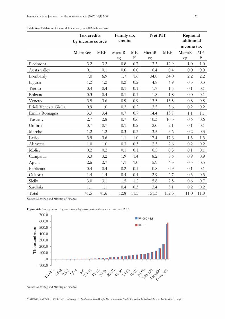
Figure A.1: Average value of gross income by gross income classes - income year 2012


-100.0

.0

100.0

200.0

300.0

400.0

500.0

600.0

700.0

Th

ou

san

d e

uro

MicroReg

MEF



Figure A.2: Average value of PIT by gross income classes - income year 2012


.0

50.0

100.0

150.0

200.0

250.0T

ho

usa

nd

eu

roMicroReg

MEF



Table A.3: VAT tax base and revenue (billion euro)

Tax base Tax revenue

Region/VAT rate 4% 10% 22% Total 4% 10% 22% Total

Piedmont 6.5 14.1 13.7 34.3 0.3 1.4 3.0 4.7

Aosta valley 0.2 0.4 0.4 1.0 0.0 0.0 0.1 0.1

Lombardy 14.5 32.2 33.7 80.4 0.6 3.2 7.4 11.2

Bolzano 0.7 1.5 1.8 4.0 0.0 0.1 0.4 0.6

Trento 0.7 1.6 1.7 4.0 0.0 0.2 0.4 0.6

Veneto 6.2 14.3 15.6 36.1 0.2 1.4 3.4 5.1

Friuli Venezia Giulia 1.7 3.8 4.2 9.6 0.1 0.4 0.9 1.4

Liguria 2.4 5.1 5.1 12.6 0.1 0.5 1.1 1.7

Emilia Romagna 5.8 13.9 15.1 34.8 0.2 1.4 3.3 4.9

Tuscany 5.2 10.9 11.8 27.9 0.2 1.1 2.6 3.9

Umbria 1.2 2.4 2.6 6.2 0.0 0.2 0.6 0.9

Marche 2.0 4.1 4.3 10.3 0.1 0.4 0.9 1.4

Lazio 8.0 17.1 19.1 44.2 0.3 1.7 4.2 6.2

Abruzzo 1.6 3.3 3.5 8.3 0.1 0.3 0.8 1.2

Molise 0.4 0.8 0.7 1.8 0.0 0.1 0.2 0.2

Campania 6.0 11.9 11.6 29.5 0.2 1.2 2.5 4.0

Apulia 4.5 9.0 8.8 22.2 0.2 0.9 1.9 3.0

Basilicata 0.6 1.3 1.3 3.2 0.0 0.1 0.3 0.4

Calabria 2.3 4.5 4.5 11.3 0.1 0.4 1.0 1.5

Sicily 5.6 10.6 10.4 26.6 0.2 1.1 2.3 3.6

Sardinia 2.1 4.1 4.3 10.5 0.1 0.4 0.9 1.4

Total 77.9 166.8 174.2 418.8 3.1 16.7 38.3 58.1 Source: MicroReg

Figure A.3: Distribution of VAT revenue by disposable income and expenditure deciles

Source: MicroReg

0

2

4

6

8

10

12

1 2 3 4 5 6 7 8 9 10

Bil

lio

n e

uro

Equivalent household disposableincome deciles

Equivalent householdexpenditure deciles



Table A.4: Test t for mean difference – EU-SILC vs HBS – Centre of Italy

EU-SILC HBS

Variable Mean Standard Deviation

Min Max Mean Standard Deviation

Min Max

Number of rooms

3.4 36.15 1 6 4.26 40.08 1 6

Loan 0.16 12.28 0 1 0.17 12.84 0 1

Number of members

2.28 39.82 1 5 2.25 40.29 1 6

Pc 0.61 16.36 0 1 0.64 16.3 0 1

Internet 0.57 16.62 0 1 0.59 16.73 0 1

Car 0.81 13.24 0 1 0.83 12.72 0 1

Dishwasher 0.51 16.77 0 1 0.61 16.59 0 1

Expenditure 23,850 363,619 7303 185,488 26,369 721,718 2,657 321,923

Number of members <5 years old

0.14 13.37 0 3 0.11 12.42 0 3

Number of members 6-17 years old

0.25 19.67 0 4 0.26 20.1 0 4


0.15 14.31 0 3 0.14 13.57 0 3


1.12 28.42 0 4 1.18 27.91 0 4

Householder with low education

0.52 16.77 0 1 0.51 16.99 0 1

Number of managers

0.02 4.9 0 2 0.03 6.57 0 3

Number of self-employed

0.05 7.87 0 3 0.08 10.53 0 3

In property 0.86 11.79 0 1 0.85 12.02 0 1

Number of earners

1.39 26.58 0 5 1.44 25.5 0 5

P-value 0.9439473 Source: our elaborations on HBS and EU-SILC



Table A.5: Test 𝝌𝟐for equality of distribution - EU-SILC vs. HBS

EU-SILC HBS

Geographical area N° % N° %

North West 7,251,965 28.3 7,270,064 28.34

North East 5,068,067 19.78 5,055,184 19.71

Centre 5,280,629 20.61 5,241,862 20.44

South 8,023,134 31.31 8,083,272 31.51

P-value 1

EU-SILC HBS

Number of components

N° % N° %

1 8,281,042 32.32 8,391,562 32.715

2 6,762,685 26.39 6,801,077 26.515

3 5,045,371 19.69 4,841,819 18.876

4 4,226,780 16.5 4,331,686 16.887

5 1,028,286 4.01 1,023,989 3.992

6 202,530 0.79 199,543 0.778

7 52,711 0.21 45,463 0.177

8 15,078 0.06 13,698 0.053

9 6,810 0.03 1,249 0.005

10 2,410 0.01 296 0.001

P-value 1

EU-SILC HBS

Number of earners

N° % N° %

0 3,956,170 15.44 2,506,273 9.95

1 13,124,349 51.22 13,378,643 53.13

2 7,109,135 27.74 8,125,715 32.27

3 1,197,490 4.67 1,009,751 4.01

4 215,988 0.84 148,021 0.59

5 20,662 0.08 13,492 0.05

P-value 0.554

EU-SILC HBS

Number of females

N° % N° %

0 3,703,284 14.45 3,868,724 15.36

1 14,672,359 57.26 14,380,843 57.11

2 5,418,932 21.15 5,315,662 21.11

3 1,615,631 6.31 1,426,684 5.67

4 191,205 0.75 171,297 0.68

5 17,507 0.07 18,684 0.07

6 4,183 0.02 n/a or 0 ? n/a or 0 ?

7 693 0 n/a or 0 ? n/a or 0 ?



P-value 1 Source: Our elaborations on HBS and EU-SILC

Table A.6: Regression of consumption on households’ characteristics

Number of observations 19,988

R squared 0.366

R- squared corr. 0.365

Variable DF Parameter

estimate

Standard

Error

T statistic

Pr > |t| Vif

Intercept 1 9.08 0.02 483.94 <.0001 0

Number of rooms 1 0.04 0 10.78 <.0001 1.26

In property 1 -0.26 0.01 -22.41 <.0001 1.17

VHS 1 0.08 0.01 9.54 <.0001 1.14

Loan 1 0.11 0.01 8.43 <.0001 1.14

Box 1 0.13 0.01 14.37 <.0001 1.22

Pc 1 0.14 0.02 8.9 <.0001 4.15

Car 1 0.27 0.01 23.11 <.0001 1.51

Internet 1 0.09 0.02 5.7 <.0001 3.81

Dishwasher 1 0.18 0.01 19.54 <.0001 1.33

Number of members <5 years old 1 0.03 0.01 2.49 0.013 1.22


1 0.03 0.01 4.26 <.0001 1.56


1 0.05 0.01 3.93 <.0001 2.41


1 -0.01 0.01 -0.74 0.461 2.19


1 0.03 0.01 3.93 <.0001 3.03

Householder with low education 1 -0.08 0.01 -5.66 <.0001 3.1

Number of males 1 0.02 0.01 2.91 0.004 2.46

Number of job seekers 1 -0.07 0.01 -5.71 <.0001 2.19

Number of retired 1 0.04 0.01 4.52 <.0001 2.39

Number of not employed 1 0 0.01 0.23 0.82 3.18

Number of managers 1 0.12 0.02 5.4 <.0001 1.06

Number of self-employed 1 0.08 0.01 5.22 <.0001 1.1

Number of members with high education

1 0.11 0.01 10.78 <.0001 2.22

Number of members with medium education

1 0.04 0.01 4.82 <.0001 3.69

Number of earners 1 0.08 0.01 7.45 <.0001 4.37 Source: Our elaborations on HBS



1 Due to data availability the model is extended to in-kind transfers only for the Region of Tuscany. 2 However, also in SHIW households’ wealth is highly under-estimated. 3 Second homes (when more than one) are considered together in the tax paid that remains after the dwelling house. This simplification should

not be a problem since second homes are basically subjected to the same taxation, independently on their number. 4 The small difference depends on the sequence of the phases of the model. Indeed, the imputation of cadastral value precedes the sample

weights calibration. 5 The data of Dipartimento delle Finanze and Agenzia del Territorio (2012) is a projection. 6 Actually in 2012 the cadastral value of the dwelling house is not included in gross income so it does not be deducted. 7 The imputation is made for each taxpayer, so in our model the number of taxpayers with positive gross income is equal to the number of

taxpayers with positive taxable income. 8 Consequently, each taxpayer has a positive tax credit. 9 Results for each Italian Region can be found in appendix (Tables A.1 and A.2). 10 The comparison on the average value of gross income by gross income classes can be found in appendix (FigureA.1). 11 The problem is detected also in Di Nicola et al. (2015). They can recover the small amounts of income within PIT and real estate datasets. 12 The average value of PIT by gross income classes can be found in appendix (Figure A.2). 13 Gastaldi et al. (2014) evaluate some VAT reforms on the integrated database built in Pisani and Tedeschi (2014). 14 Tax base and tax revenue for each Region is reported in appendix (Table A.3). In appendix it is also shown the distribution of tax revenue by

income and expenditure deciles (Figure A.3). 15 Table 10 “Imposte indirette prelevate dalle Amministrazioni pubbliche e dall'Unione europea per tipo di tributo. Anni 1995 - 2015 (milioni di

euro correnti)”. 16 See Bianchini et al.(2013) for a previous application. 17 The education module can be easily extended to the rest of Italy. For health data are available only for Tuscany. 18 Data are taken from Comitato Nazionale di Valutazione del Sistema Universitario (CNVSU). 19 The services for which regional data are available do not cover the entire public health expenditure. Prevention, homecare, assistance against

addiction, mental health assistance, primary and district care are excluded. 20 Sonedda and Turati (2005) find a regressive but weak and not highly significant impact of health expenditure. They follows the insurance value

approach.

NOTES

Date post:	08-Sep-2018
Category:	Documents
Upload:	trinhhuong
View:	220 times
Download:	0 times

Microreg: a Traditional Tax-Benefit Microsimulation Model ... · INTERNATIONAL JOURNAL OF...

Documents