12
Microsegregation Models and their Role In Macroscale Calculations Vaughan R. Voller University of Minnesota
| Date post: | 31-Dec-2015 |
| Category: |
Documents |
| Upload: | nicholas-phelps |
| View: | 44 times |
| Download: | 1 times |
Microsegregation Models and their RoleIn Macroscale Calculations
Vaughan R. Voller University of Minnesota
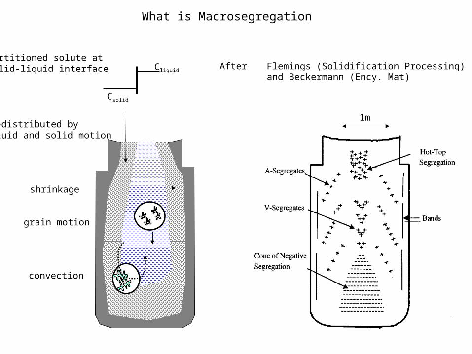
After Flemings (Solidification Processing) and Beckermann (Ency. Mat)
1m
l
TLe
What is Macrosegregation
Csolid
Cliquid
Partitioned solute atsolid-liquid interface
Redistributed by Fluid and solid motion
convection
grain motion
shrinkage
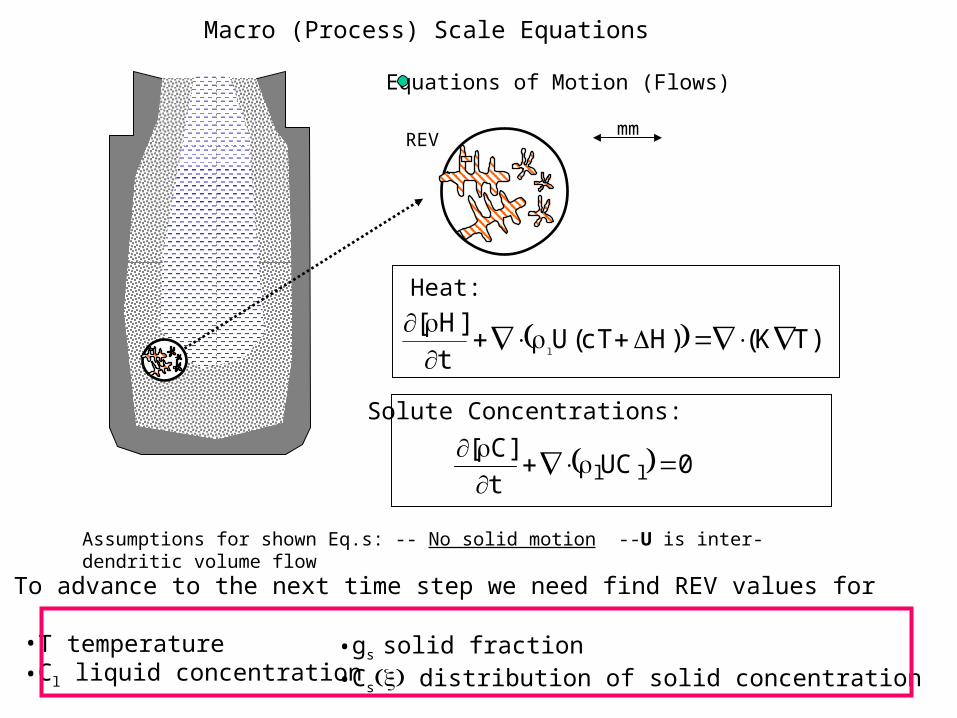
Macro (Process) Scale Equations
Equations of Motion (Flows)
mmREV
Heat:
)TK()HcT(Ut
]H[l
0UCt
]C[ll
Solute Concentrations:
Assumptions for shown Eq.s: -- No solid motion --U is inter-dendritic volume flow To advance to the next time step we need find REV values for
•T temperature•Cl liquid concentration
•gs solid fraction•Cs distribution of solid concentration
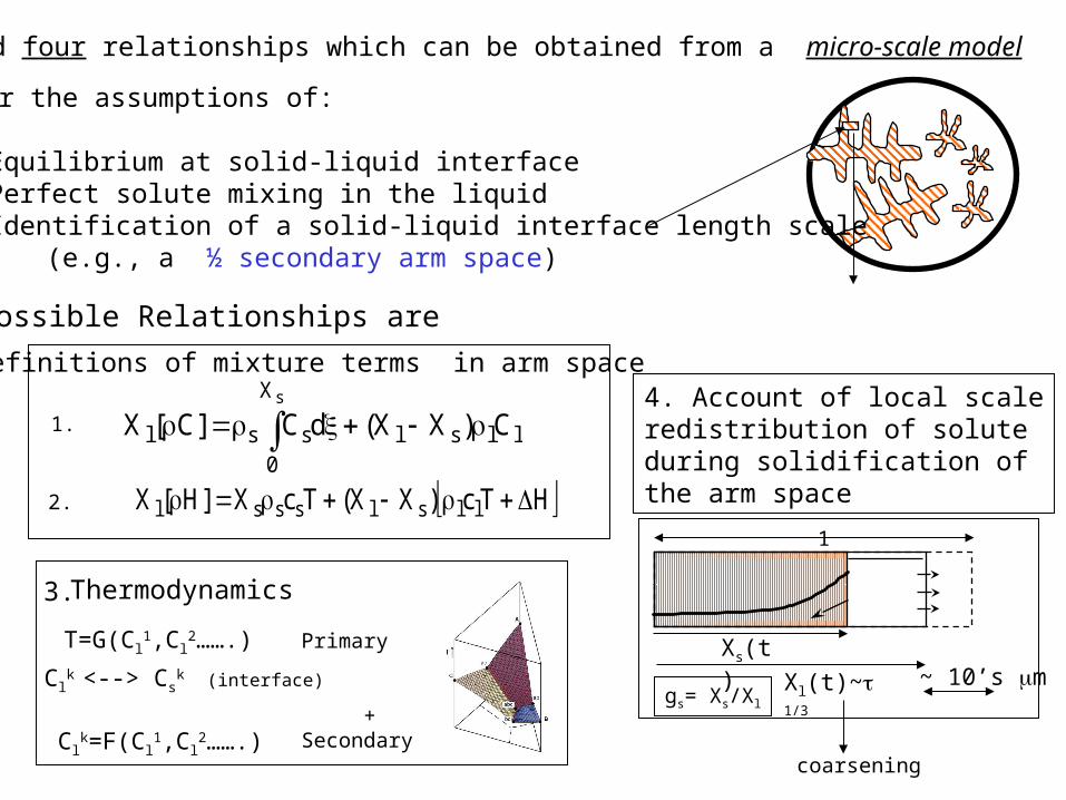
Need four relationships which can be obtained from a micro-scale model
Under the assumptions of:
1. Equilibrium at solid-liquid interface2. Perfect solute mixing in the liquid3. Identification of a solid-liquid interface length scale (e.g., a ½ secondary arm space)
Possible Relationships are
Xs(t)
Xl(t)~1/3 ~ 10’s m
coarsening
llsl
X
0ssl C)XX(dC]C[X
s
HTc)XX(TcX]H[X llslsssl
Definitions of mixture terms in arm space
T=G(Cl1,Cl
2…….)
4. Account of local scaleredistribution of soluteduring solidification ofthe arm space
3.
1
1.
2.
Thermodynamics
Primary
+Secondary
Clk <--> Cs
k (interface)
Clk=F(Cl
1,Cl2…….)
gs= Xs/Xl
solidLiquid
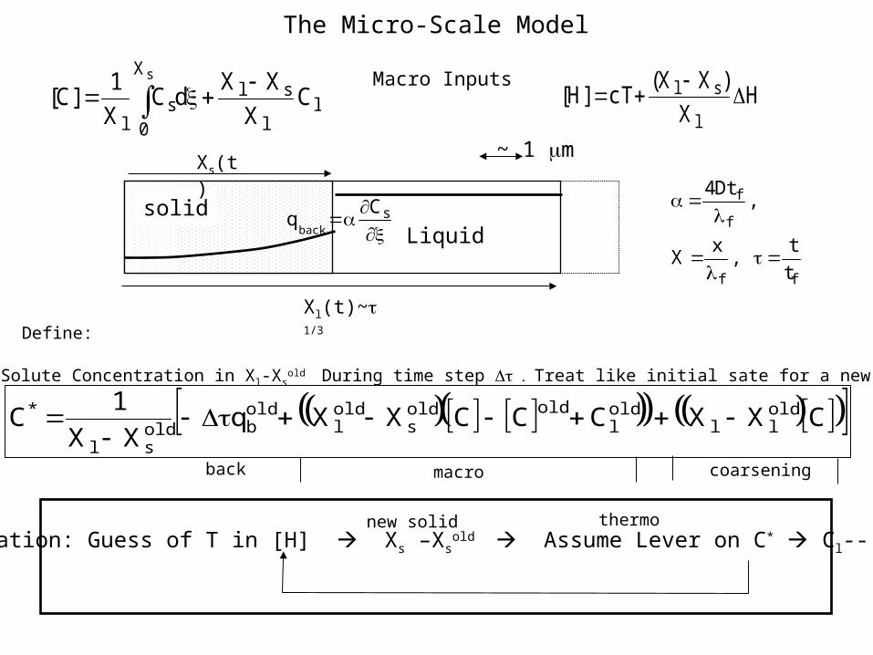
The Micro-Scale Model
~ 1 m
ll
slX
0s
lC
X
XXdC
X
1]C[
s H
X
)XX(cT]H[
l
sl
Macro Inputs
Xs(t)
Xl(t)~1/3
sCq
back
Define:
CXXCCCXXqXX
1C old
lloldl
oldolds
oldl
oldbold
sl
*
macro coarseningback
Average Solute Concentration in Xl-Xsold During time step Treat like initial sate for a new problem
Iteration: Guess of T in [H] Xs –Xsold Assume Lever on C* Cl--, T
new solid thermo
ff
f
f
t
t,
xX
,Dt4
s2s
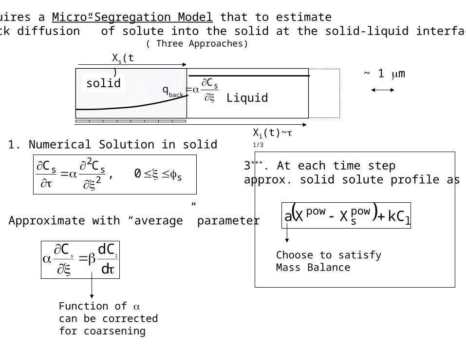
2s 0,
CC
3***. At each time stepapprox. solid solute profile as
lpows
pow kCXXa
Choose to satisfyMass Balance
1. Numerical Solution in solid
Requires a Micro-Segregation Model that to estimate “back diffusion” of solute into the solid at the solid-liquid interface
solidLiquid
~ 1 mXs(t)
Xl(t)~1/3
sCq
back
( Three Approaches)
d
dCCls
2. Approximate with “average” parameter
Function of can be correctedfor coarsening

solid
Testing: Binary-Eutectic Alloy. Cooling at a constant rate
Predictions of Eutectic Fraction at end of solidification
0.1
0.11
0.12
0.13
0.14
0.15
0.16
0.17
0.18
0.001 0.01 0.1 1 10
Fourier Number
Fra
cti
on
Eu
tec
tic
coarseningNumerical back diff model
Approx profile model
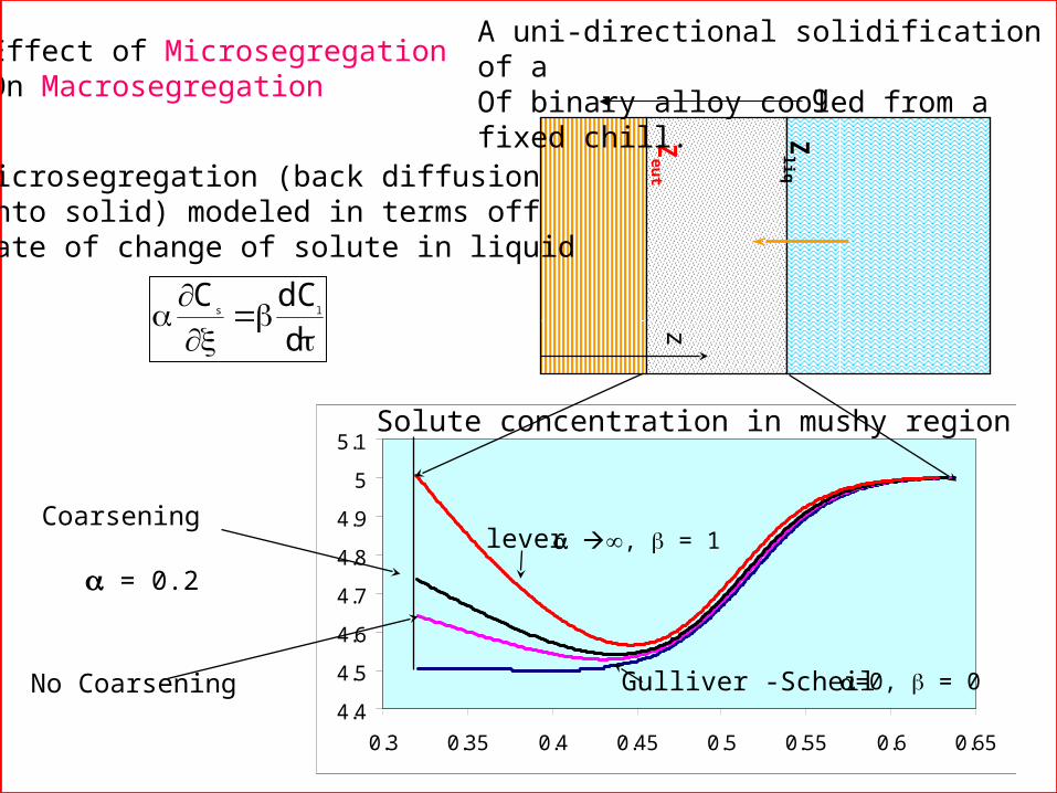
4.4
4.5
4.6
4.7
4.8
4.9
5
5.1
0.3 0.35 0.4 0.45 0.5 0.55 0.6 0.65
zZ
eut
Zliq
lever
Gulliver -Scheil
Effect of MicrosegregationOn Macrosegregation
= 0.2
Coarsening
g
A uni-directional solidification of a Of binary alloy cooled from a fixed chill.
Microsegregation (back diffusion into solid) modeled in terms off rate of change of solute in liquid
ddCC
ls
No Coarsening
, = 1
=0, = 0
Solute concentration in mushy region
l
TLe
~ 1 mm
ll
slX
0s
lC
X
XXdC
X
1]C[
s
HX
)XX(cT]H[
l
sl
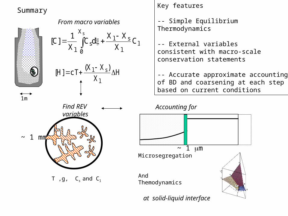
1m
Summary
T ,g, Cs and Cl
~ 1 m
solid
Microsegregation
And Themodynamics
From macro variables
Find REVvariables
Accounting for
at solid-liquid interface
Key features
-- Simple Equilibrium Thermodynamics
-- External variablesconsistent with macro-scaleconservation statements
-- Accurate approximate accounting of BD and coarsening at each stepbased on current conditions
l
TLe
1m
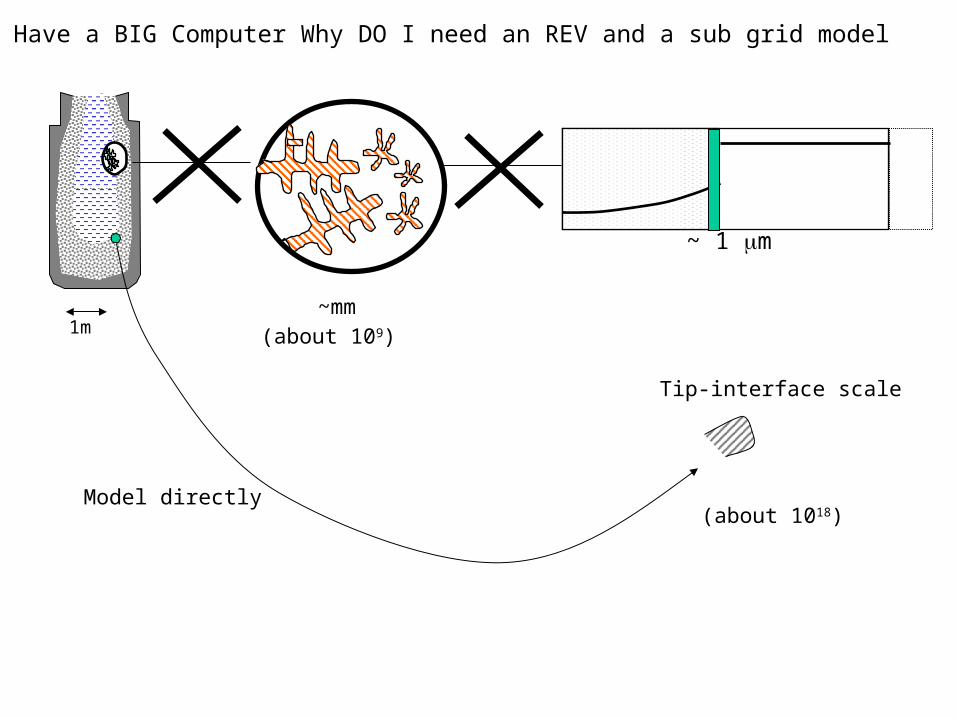
I Have a BIG Computer Why DO I need an REV and a sub grid model
~ 1 m
solid
~mm(about 109)
Model directly (about 1018)
Tip-interface scale
1.0E+02
1.0E+04
1.0E+06
1.0E+08
1.0E+10
1.0E+12
1.0E+14
1.0E+16
1.0E+18
1.0E+20
1.0E+22
1.0E+24
1.0E+26
0 20 40 60 80 100 120
Year-1980
No
de
s
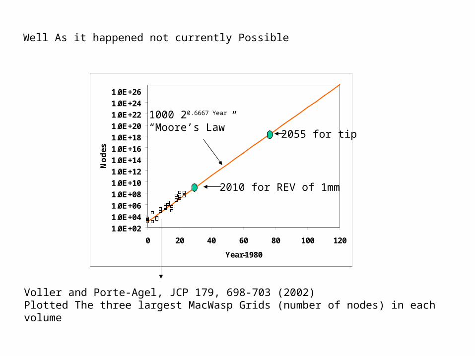
Well As it happened not currently Possible
1000 20.6667 Year
“Moore’s Law”
Voller and Porte-Agel, JCP 179, 698-703 (2002) Plotted The three largest MacWasp Grids (number of nodes) in each volume
2010 for REV of 1mm
2055 for tip
xxllME
xU
)g1(xx
p)g1()U()U(
t
U
yyravlllMEg)g1(
yV
)g1(yy
p)g1()V()V(
t
U
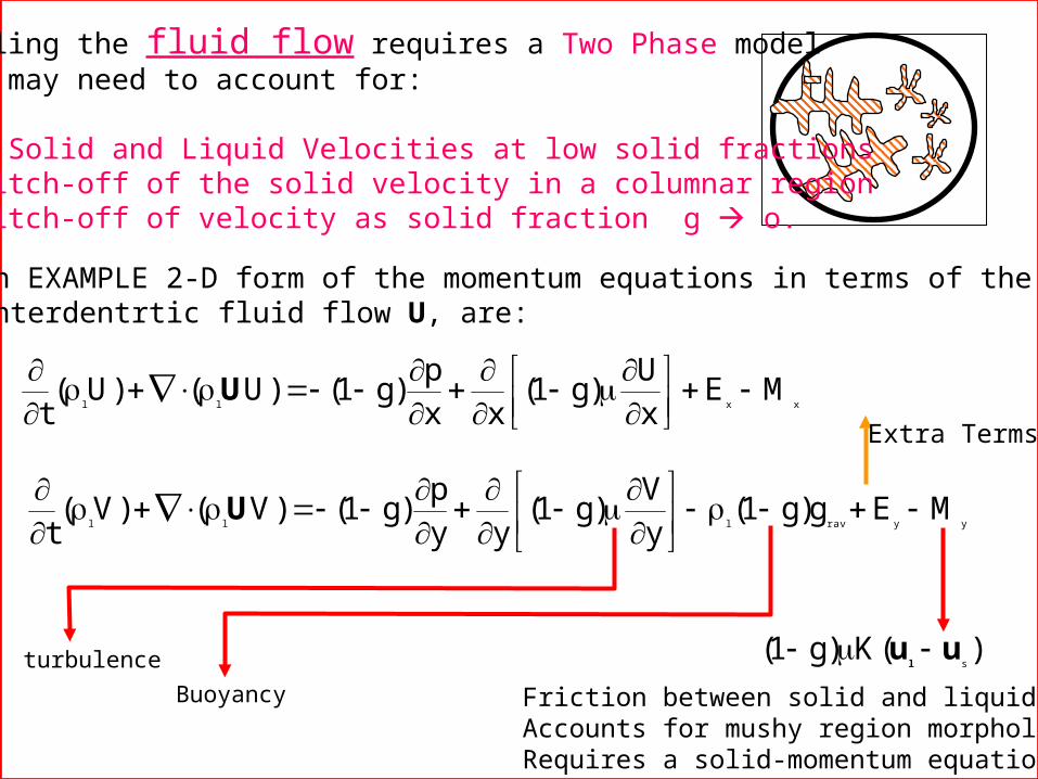
Modeling the fluid flow requires a Two Phase modelThat may need to account for:
Both Solid and Liquid Velocities at low solid fractionsA switch-off of the solid velocity in a columnar regionA switch-off of velocity as solid fraction g o.
An EXAMPLE 2-D form of the momentum equations in terms of the interdentrtic fluid flow U, are:
turbulence
Buoyancy
)(K)g1(suu
l
Friction between solid and liquidAccounts for mushy region morphologyRequires a solid-momentum equation
Extra Terms


