MICROSOFT EXCEL 2010 - Massey

LEARNING

GUIDE

INFORM A TION TECHNOLOGY SERVICES

MICROSOFT EXCEL 2010

Level 3 PivotTables & Charts

Information Technology Services Microsoft Excel Pivot Tables and Charts 2010 Learning Guide

Page 2 of 41

Course Overview

Welcome Information Technology Services is happy to provide you with this training opportunity. We hope that you enjoy it and the time you invest in participating is valuable to your work here at Massey University.

Feedback Upon course completion please fill out the online ITS Course Evaluation form. Your feedback is confidential and the information you provide allows us to deliver relevant and high quality ITS training for staff.

Purpose To provide a guide to new users of Pivot Charts and Tables.

Learning outcomes

By the end of this course you will be able to:

Create and use a Pivot Chart and Table.

Work with Pivot Table data.

Use Slicers and Report Filters.

Consolidate data from multiple ranges.

Format Pivot Tables and Charts.

Apply Conditional Formatting to Pivot Tables.

Format Face to Face Learning

Learning guide Please return printed material to the Trainer at the end of the session.

A digital copy of this document is available online.

ITS thanks you for considering the environment before printing.

Help & information

For help or information in addition to what is provided in this training please visit:


Page 3 of 41

Microsoft Excel

Pivot Tables and Charts User Guide

1. Creating a PivotTable ................................................................................................ 5

Introduction ................................................................................................................ 5

Parts of a PivotTable .................................................................................................. 5

Creating a PivotTable ................................................................................................ 6

Build the PivotTable .................................................................................................. 7

Add data to the table .................................................................................................. 7

Other customisation options ...................................................................................... 8

2. Working with Data ..................................................................................................... 9

Data Field Summary Options..................................................................................... 9

Summarise by Averages ............................................................................................ 9

Changing Displayed Values ..................................................................................... 10

Changing Displayed Values, continued ................................................................... 11

Calculated Fields ...................................................................................................... 12

3. Sorting and Filtering Data ........................................................................................ 14

Introduction .............................................................................................................. 14

Sorting Data ............................................................................................................. 14

Using Filters ............................................................................................................. 14

Filtering by Selection ............................................................................................... 15

Filtering by Rule ...................................................................................................... 16

Using Rule filters ..................................................................................................... 16

Search Filters ........................................................................................................... 17

Using Search Filters ................................................................................................. 17

4. Slicers and Report Filters ......................................................................................... 18

Slicers ....................................................................................................................... 18

Using Slicers ............................................................................................................ 18

Formatting Slicers .................................................................................................... 20

Classic PivotTable Layout ....................................................................................... 21

Report Filters ........................................................................................................... 22

Using Report Filters ................................................................................................. 22

5. Consolidating Data from Multiple Ranges .............................................................. 23

Introduction .............................................................................................................. 23

Identical Structures .................................................................................................. 23

PivotTable and PivotChart Wizard .......................................................................... 23

6. Formatting a PivotTable .......................................................................................... 25


Page 4 of 41

Introduction .............................................................................................................. 25

Selecting a Style ....................................................................................................... 25

Changing the Layout ................................................................................................ 25

Inserting Blank Rows ............................................................................................... 25

Report Layouts ......................................................................................................... 26

Report Layouts, continued ....................................................................................... 27

Changing the number format ................................................................................... 27

7. Applying Conditional Formatting ............................................................................ 28

Introduction .............................................................................................................. 28

Highlight Cells Rules ............................................................................................... 28

Top/Bottom Rules .................................................................................................... 29

Data Bars .................................................................................................................. 29

Color Scales ............................................................................................................. 29

Icon Sets ................................................................................................................... 30

Editing Conditional Formats .................................................................................... 30

Multiple Conditions ................................................................................................. 30

Controlling Multiple Rules ...................................................................................... 31

Deleting Conditional Formats .................................................................................. 32

8. Creating and Manipulating a Pivot Chart ................................................................ 33 Introduction .............................................................................................................. 33

Create a PivotTabel with a PivotChart..................................................................... 33

Creating a PivotChart from an Existing PivotTable ................................................ 34

Moving a PivotChart ................................................................................................ 35

Pivoting and Filters .................................................................................................. 36

Formatting a PivotChart ........................................................................................... 36

PivotChart Layouts .................................................................................................. 38

Changing the Layout ................................................................................................ 38

PivotChart Types ..................................................................................................... 38

Changing Chart Type ............................................................................................... 38

Changing Chart Type, continued ............................................................................. 39

Trend lines ............................................................................................................... 41

Creating a Trend Line .............................................................................................. 41


Page 5 of 41

1. Creating a PivotTable

Introduction The aim of a PivotTable is to create a report.

A PivotTable is used as an interactive worksheet table that allows you to

quickly summarise large amounts of data using the format and calculation

method specified by you. The name refers to the table’s ability to rotate

rows and columns headings to access and present different perspectives of

your data.

When creating a PivotTable, you will be asked to specify the data to be

used as row fields, column fields and page fields.

Parts of a

PivotTable The following table describes the terms used to describe different aspects of

the PivotTable.

Part Function

Fields Categories of data such as rows or columns.

Items These are sub-categories.

Data area The data to be summarised.

Layout The arrangement of the fields within the table.

Page Fields Also known as a Report Filter field. A field

that you can use to filter your PivotTable.

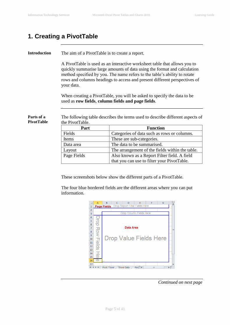
These screenshots below show the different parts of a PivotTable.

The four blue bordered fields are the different areas where you can put

information.

Continued on next page


Page 6 of 41

1. Creating a PivotTable, continued

Parts of a

PivotTable,

continued

The PivotTable Field List shows the available fields that you can add to the

table. These are based on the column headings in your original worksheet.

Creating a

PivotTable The following table describes the steps to take in order to create a

PivotTable.

Step Action

1 Select Insert > PivotTable (from the Tables group).

2 a) Use the top set of radio buttons to choose where the

data for you PivotTable will come from. Either

click into the table before you start building your

PivotTable, or select your data from here.

b) Use the bottom radio button to place the pivot table

in a new worksheet or the existing worksheet.

c) Click on OK.

Note: You must specify data before you can move to the next

option.



Page 7 of 41


Build the

PivotTable Once you create a pivot table a new (or existing) worksheet will be

displayed showing the empty table.(i.e. the template)

Add data to the

table Drag and drop items from the PivotTable Field List into the four areas

below the list.

The locations you choose to drop the items will control what information

the table displays and where it is displayed.

You can also select the tick box next to the field name to add it to the

PivotTable.

The Row Labels and Column Labels are the row and column headings.

The Values area is the actual information that will be measured. (E.g.

count, totals, averages etc. …).



Page 8 of 41


Other

customisation

options

You can remove fields from the table by dragging them out of the four

areas, or un-tick them in the field list

You can drag fields from one area to another if required.

You can add more than one field to any area.


Page 9 of 41

2.Working with Data

Data Field

Summary

Options

PivotTables allow you to perform different summary calculations. You can

also choose the type of values to be shown in the data area.

Summarise by

Averages To change the way data is summarised in the PivotTable, right click a data

cell in the table (Note: Do not select a label, total, or subtotal field). Then

from the shortcut menu select a suitable option.



Page 10 of 41

Working with Data, continued

Changing

Displayed

Values

In addition to be able to change how data is summarised, you can also

choose how data is displayed in a PivotTable.

Show Values As This feature allows you to present values in different ways.

Step Action

1



Page 11 of 41

Working with DataContinued on next page, continued

Changing

Displayed

Values,

continued

Step Action

2 Select % of. This displays values as a percentage of the value

of the Base item in the Base field.

3 The options selected below will display each month as a

percentage of the previous month.

4 The displayed items will look similar to the image below.

5 Select Running Total in. This displays the value for

successive items in the Base field as a running total

If I chose Month as my base field, this is how it would look.



Page 12 of 41


Calculated

Fields You can create custom fields that summarise PivotTable data using a

formula.

Step Action

1 Select PivotTable Tools > Options > Field, Items, & Sets

(from the Calculations group)

2 From the drop down list select Calculated Field.

3 In the Name field type the name you want for your calculated

field. (i.e. Average Sale.)

4 Create your calculation (i.e. revenue as a % of sales count) by

clicking into the Formula field after the equals sign. Then

select the appropriate field from the list of Fields by clicking

the Insert Field button.

5 Now click back into the Formula field and type your

mathematical operator (i.e. +, -, /, *).

6 Repeat steps 4 and 5 as appropriate.

7 Select OK when you have finished.



Page 13 of 41


Refreshing data Once you have created your PivotTable and the source data changes you

will need to refresh your PivotTable.

Refresh

Options Choose the correct refresh option from the table below.

If your source data

is

Then ...

An Excel table Under PivotTable Tools > Options click

Refresh.

An Excel list Under PivotTable Tools > Options click

Change Data Source, and ensure that the

Table/Range is correct.


Page 14 of 41

3.Sorting and Filtering Data

Introduction Sorting allows you to change the order in which your data appears. Filters

allow you to view a subset of your data.

Sorting Data 1. Click any cell in the row and column of the PivotTable you want to

sort.

2. Under PivotTable Tools > Options (Sort and Filter group) select

a sort option.

Using Filters There are 3 different ways you can use filters:

Filtering by Selection.

Filtering by Rule.

Filtering by Search Term.



Page 15 of 41

Sorting and Filtering Data, continued

Filtering by

Selection With this method you select the value you want to display.

Each area of your pivot table will show a pale blue heading. These

headings usually contain a drop down arrow that you can use to restrict

your display to particular items.

You can achieve the same result by moving your mouse cursor over the

field you want to filter by in the PivotTable Field List and clicking the

drop down arrow that appears, to make a selection.

Note:

Tick the Select All checkbox before

you move this field to another location.

If you move a filtered list it will remain filtered in the new location.

You can filter by more than one field at a time.

To clear all filters in a PivotTable, click on Options > Clear > Clear

Filters.



Page 16 of 41


Filtering by

Rule If the data you want to filter by fits a rule (e.g. all values > 1000), you can

create a rule to filter you data.

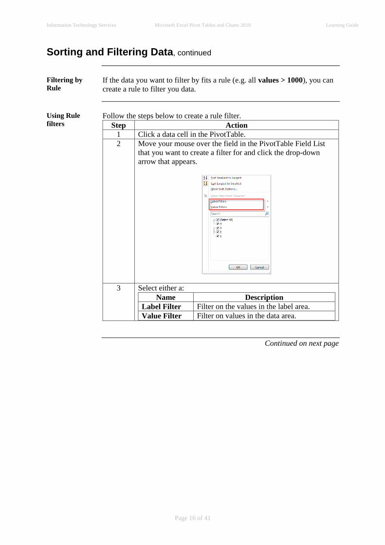
Using Rule

filters Follow the steps below to create a rule filter.

Step Action

1 Click a data cell in the PivotTable.

2 Move your mouse over the field in the PivotTable Field List

that you want to create a filter for and click the drop-down

arrow that appears.

3 Select either a:

Name Description

Label Filter Filter on the values in the label area.

Value Filter Filter on values in the data area.



Page 17 of 41


Search Filters Search Filters can be used to locate a string of characters in your data.

Using Search

Filters Follow the steps below to use a Search Filter.

Step Action

1 Move your mouse over the field in the PivotTable Field List

that you want to create a filter for and click the drop-down

arrow that appears.

2 In the search field type the search characters that you are

looking for.

3 You can add subsequent criteria to the current search criteria

by typing in the new criteria and selecting the option Add

current selection to filter.


Page 18 of 41

4.Slicers and Report Filters

Slicers Slicers provide buttons you can click to filter PivotTable data. In addition

to quick filtering, Slicers also indicate the current filtering state.

Using Slicers Follow the steps below to use Slicers.

Step Action

1 Click a data cell in the PivotTable.

2 Select PivotTable Tools > Options > Insert Slicer (Sort &

Filter group).

3 You can use the table below to select and clear filters on your

Slicer.

If ... Then ...

You want to select multiple

non-adjacent fields

Keep the Ctrl button down

and left click non-adjacent

fields.

You want to select multiple

adjacent fields.

Click the first field, then

keeping the Shift button

down, left click the last field

You want to clear all filters. Click the clear filter button

on the top right hand corner

of the Slicer.



Page 19 of 41

Slicers and Report Filters, continued

Using Slicers,

continued

4 You can resize and reposition Slicers by dragging and

dropping them.

5 You can insert Slicers for as many fields as you want to.

Typically Slicers don’t work well for fields that have more

than 20 unique values.

6 To remove a Slicer, right click it, and from the shortcut menu

select Remove Month (or whatever the field name happens to

be.)



Page 20 of 41


Formatting

Slicers You can format Slicers so that they are visually distinctive from the

PivotTable. To format a Slicer follow the steps below:

Step Action

1 Click on the Slicer to make it active. (Once active you will see

a selection border around it).

2 Click on the Options contextual tab that appears.

3 Select a style form the Styles Gallery.

4 To type in a new caption for the Slicer, click on Options and

under Slicer Captions, type in a new caption.



Page 21 of 41


Classic

PivotTable

Layout

By enabling Classic PivotTable Layout you can drag fields directly onto

the PivotTable. Classic Layout also allows you to drag fields off the

PivotTable, and move fields from one part of the PivotTable to another. To

enable Classic Layout, right click any part of the PivotTable and from the

shortcut menu select PivotTable Options. Select the Display tab and tick

the checkbox next to Classic PivotTable layout.



Page 22 of 41


Report Filters Report Filters allow you to filter your data without having to change the

structure of your PivotTable.

Using Report

Filters If you have a large amount of data and would like to organise the

information into multiple PivotTables, you can break the data down into

pages. These pages are really nothing more than filters for the entire table.

o At the top of your PivotTable should be a section labelled

Drop Report Filter Field Here (Note: classic PivotTable

layout is enabled). Drag the field to be used for filtering the

data to this section, or drag it to the section labelled Report

Filter on the task pane.

o The field will have a pull-down list that can be used to show

either all of the data or individual items. Simply select the

item to be shown in the current table from this pull-down

list.

o To create a separate worksheet for each PivotTable, select

PivotTable Tools > Options > Options (in the PivotTable

group) > Show Report Filter Pages.

o A small box will be displayed showing the field on which

each PivotTable will be based.


Page 23 of 41

5.Consolidating Data from Multiple Ranges

Introduction You can create a Pivot Table, using data from different sheets in a

workbook, or from different workbooks, if those ranges have identical

column and row structures.

Identical

Structures The ranges must all contain the same row and column titles and be laid out

in tabular (rectangular) format, without any blank cells.

.

PivotTable and

PivotChart

Wizard

We will use the Wizard to consolidate our ranges.

Step Action

1 Activate the Wizard by typing Alt + d then p.

2 The PivotTable and PivotChart wizard will appear.

3 Select the radio button for Multiple consolidation ranges.

Click Next.



Page 24 of 41

Consolidating Data from Multiple Ranges, continued

PivotTable and

PivotChart

Wizard,

continued

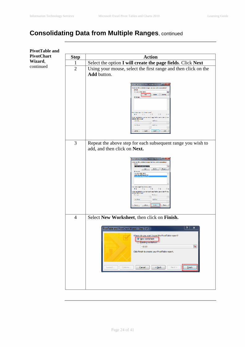
Step Action

1 Select the option I will create the page fields. Click Next

2 Using your mouse, select the first range and then click on the

Add button.

3 Repeat the above step for each subsequent range you wish to

add, and then click on Next.

4 Select New Worksheet, then click on Finish.


Page 25 of 41

6.Formatting a PivotTable

Introduction Once the PivotTable has been created, you can change the look of the table

just as you would any other cells within your worksheet.

Selecting a

Style Follow the steps below to change the style.

Step Action

1 Click into the PivotTable so that it is selected.

2 Under the PivotTable Tools contextual tab select the Design

tab and then the drop down arrow to the right of PivotTable

Styles.

3 From the list select the desired style for your table.

Changing the

Layout You are able to change PivotTable layouts by inserting blank rows and

choosing from three report layouts.

Inserting Blank

Rows Select PivotTable Tools > Design > Blank Rows (in the Layout group),

and choose an option.



Page 26 of 41

Formatting a PivotTable, continued

Report Layouts Select PivotTable Tools > Design > Report Layout (in the Layout

group), and choose an option.



Page 27 of 41

Formatting a PivotTable, continued

Report

Layouts,

continued

Changing the

number format Select a data cell in the PivotTable, right click and from the shortcut menu

select Number Format.

Under Number > Category you are able to choose whether to use a 1000

separator and the number of decimal places you want to display.


Page 28 of 41

7.Applying Conditional Formatting

Introduction Formats that change the appearance of a cell’s contents by applying rules

are called conditional formats. This makes it easy to find a cell as its

appearance is based on its value. The formats will change position when

you alter the PivotTable.

Highlight Cells

Rules You can use the steps below to apply conditional formatting rules.

Step Action

1 Click a data cell in the PivotTable that you want to apply a rule

to.

2 Select Home > Conditional Formatting (from the Styles

group), > Highlight Cells Rules.

3 Once you have created a rule you can choose how the rule will

be applied. Click the options button to the right of the cell and

this will allow you to choose which cells you want to apply the

rule to.

The options radio button works as follows:

Part Function

Selected cells Only the cell that you highlighted.

Sum of Revenue values.

This includes all data in the main data

area, as well as totals and subtotals.

Sum of Revenue

values for Month

and Company

This includes all data in the main data

area, but excludes totals and subtotals.



Page 29 of 41

Applying Conditional Formatting, continued

Top/Bottom

Rules This type of conditional formatting allows you to identify the top or bottom

values in a PivotTable.

Select Home > Conditional Formatting (from the Styles group), >

Top/Bottom Rules. You can create 2 types of conditional formats:

1. Formats that identify a certain number of top and bottom values.

2. Formats that identify top and bottom values based on a

percentage.

Data Bars To get an idea of how 2 or more numbers compare you can use data bars.

This adds colour bars to a cell’s background, where the length of the bar

reflects the relative value in the cell.

Select Home > Conditional Formatting (from the Styles group), > Data

bars. You can choose between:

1. Gradient Fill – tapers off to the right, so it’s a bit harder to tell

what their value is.

2. Solid Fill – doesn’t taper off and is the recommended option.

Note: Because data bars fill a % of cells interior and don’t have a fixed

length, two cells with the same value can have data bars of different

lengths. In this case choose Outline Form as your report layout so that

columns have the same widths, (Design (Contextual Tab) > Report

Layout > Show in Outline Form).

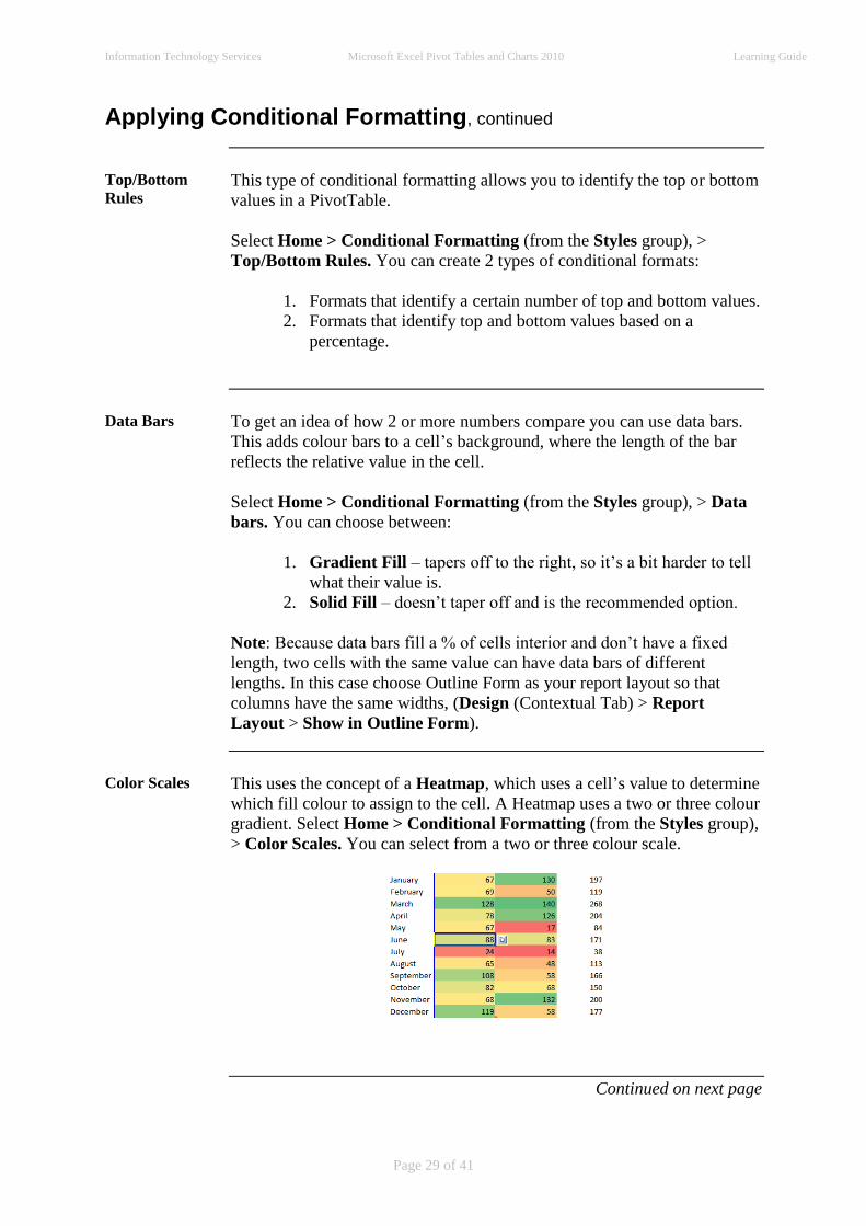
Color Scales This uses the concept of a Heatmap, which uses a cell’s value to determine

which fill colour to assign to the cell. A Heatmap uses a two or three colour

gradient. Select Home > Conditional Formatting (from the Styles group),

> Color Scales. You can select from a two or three colour scale.



Page 30 of 41


Icon Sets Icon Sets can provide useful information about large datasets, but they

come into their own when you use them to summarise a small amount of

data. If you setup your workbook as a dashboard that summarises

performance then you can use indicators such as red, orange and green to

indicate acceptable, unacceptable and excellent results. Select Home >

Conditional Formatting (from the Styles group), > Icon Sets.

Editing

Conditional

Formats

To change the format rules, follow the steps below.

Step Action

1 Click on any cell in the PivotTable that has conditional

formatting applied.

2 Click Home > Conditional Formatting > Manage Rules.

3 Click on the rule that you want to edit and then click onto the

Edit Rule button.

4 In this dialogue box you can change anything about the rule

including the type of rule, the cells to which it is applied, and

the rule’s conditions.

Multiple

Conditions In Excel 2010 there is no limit to the number of conditional formatting

rules you can apply. It is also possible for more than one conditional

formatting rule to be applied at the same time.



Page 31 of 41


Controlling

Multiple Rules To manage a number of conditional formatting rules:

Step Action

1 Click Home > Conditional Formatting > Manage Rules.

2 In the Rules Manager make sure that This PivotTable is

selected.

3 Excel 2010 does not stop checking conditions unless you tell it

to, by clicking the Stop If True checkbox.

4 You can change the order in which Excel applies these rules.

Select the rule you want to move, and then click the move up

or down arrow.



Page 32 of 41


Deleting

Conditional

Formats

You can delete conditional formats in two ways:

When ... Then ...

You want to

delete

individual

rules.

Use the rule manager, (Home > Conditional

Formatting > Manage Rules) to select the rule, and

then press the Delete Rule button.

You want to

remove a

particular set

of conditional

formats.

Select Home > Conditional Formatting > Clear

Rules.


Page 33 of 41

8.Creating and Manipulating a Pivot Chart

Introduction Charts summarise data visually. Pivot Charts are linked to a PivotTable. By

using a PivotTable as the basis for your chart, you can quickly rearrange

the data that is displayed in the chart. There are two ways to create a

PivotChart:

3. Creating a PivotTable and PivotChart at the same time.

4. Creating a PivotChart from an existing PivotTable.

Create a

PivotTabel with

a PivotChart

Follow the steps below to create both at the same time.

Step Action

1 Make sure your data is laid out as a list or table.

2 Click a cell in the list.

3 Select Insert > PivotTable (Tables Group) > PivotChart.

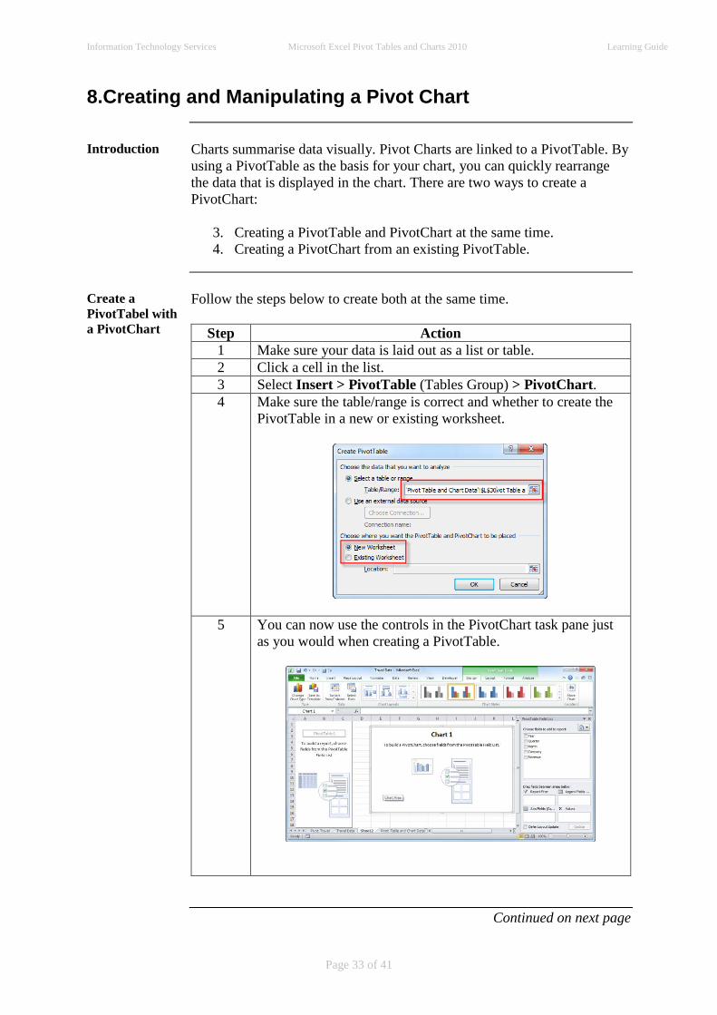
4 Make sure the table/range is correct and whether to create the

PivotTable in a new or existing worksheet.

5 You can now use the controls in the PivotChart task pane just

as you would when creating a PivotTable.



Page 34 of 41

Creating and Manipulating a Pivot Chart, continued

Create a

PivotTabel with

a PivotChart,

continued

Step Action

1 For example to create a column chart of yearly revenues:

Step Action

1 Drag the Revenue field to the Values area.

2 Drag the Year field to the Legend Fields area.

3 Note:

Legend Fields (Series) = Column Area (PivotTable)

Axis Fields (Categories) = Row Area (PivotTable).

Every unique value in any field within the Legend

Fields area will have a separate line or bar or column

on the body of the chart.

.

Creating a

PivotChart

from an

Existing

PivotTable

Follow the steps outlined below.

Step Action

1 Select the PivotTable by clicking into it.

2 As an example select > Insert > Column (Charts group) > 2-

D Column > Clustered Column.



Page 35 of 41


PivotCharts vs.

Ordinary

Charts

The following table explains the differences between PivotCharts and

ordinary charts.

Step Action

1 With PivotCharts you can’t switch the row and column

orientation by using the Select Data Source dialog box. You

can however overcome this by pivoting the PivotChart.

2 You can’t create xy scatter charts, stock charts or bubble

charts.

3 Refreshing a PivotChart removes trend lines, data labels, error

bars, and a few other settings.

Moving a

PivotChart It’s often easier to view and manipulate a PivotChart if it’s on a separate

worksheet. To move the PivotChart to a new worksheet you can:

Step Action

1 Click on the PivotChart to select it.

2 Select PivotChart Tools > Design > Move Chart. (under

Location).

3 Select the New Sheet radio button.



Page 36 of 41


Pivoting and

Filters You can click onto either the PivotTable or the PivotChart to manipulate

the PivotChart data.

PivotChart filters are created and used in the same way as PivotTable

filters.

Formatting a

PivotChart First click onto the PivotChart, then you can format it in a number of ways:

Part Action

To

change

the

style.

Select PivotChart Tools > Design > more arrow to the right

of chart styles. This will open the Styles Gallery from which

you can select a style.



Page 37 of 41


Formatting a

PivotChart,

continued

Formatting individual elements.

Step Action

1 First select the element you want to apply the

formatting to. You can select an element in one of

two ways:

1. Move your mouse over that element. (You

will see a screen tip pop up) then left click to

select the chart element.

2. Use the Chart Elements list to select an

element by selecting PivotChart Tools >

Format > and the elements drop down arrow

(in the Current Selection group)

2 Once the element has been selected, click on the

Format contextual tab to change the formatting of

the particular item.

3 To format a single data point in a data series, click

the series once to select all the elements in the series.

Then click the element a second time to select that

single element.



Page 38 of 41


PivotChart

Layouts When creating a PivotChart, Excel uses a basic layout to determine what

elements of the chart to display and where those elements will be displayed

on the chart. An element could be a chart title, a legend, or axis titles and

labels.

Changing the

Layout To change a chart’s layout you can:

Select a chart from the Chart Layouts gallery by selecting PivotChart

Tools > Design and then the more button at the bottom of the Chart

Layouts gallery.

Change individual layout options by clicking on the chart and then

selecting PivotChart Tools > Layout.

PivotChart

Types Your data could be presented by more than one chart type. You can’t create

an XY scatter chart, a stock chart or a bubble chart using PivotTable data.

Changing

Chart Type Click onto the PivotChart to activate it. Select PivotChart Tools > Design

> Change Chart Type. A Change Chart Type dialogue box will be

displayed, allowing you to select a particular chart type.



Page 39 of 41


Changing

Chart Type,

continued

Chart

Type

Used for

Line

Chart

Displaying continuous data over time. Good for showing

trends in data as long as the data was captured in equal

intervals.

Pie

Chart

Showing the share of a total contributed to by the individual

data values in a single data series.

Bar

Chart

Summarising data when the axis labels are long and the values

shown are durations.

Area

Chart

Same as the line chart but the entire area under the line is filled

in. The chart emphasises the magnitude of change over time

and also how much each data element contributes to the total

for a given measurement.



Page 40 of 41


Changing

Chart Type,

continuedcontin

ued

Surface

Charts

Mainly used for scientific data (e.g. to find the optimal

combination of two datasets such as rainfall and crop

production).

Radar

Charts

Used for determining the aggregate values of several data

series.



Page 41 of 41


Trend lines Trend lines help you visualise/predict future trends in your data.

Creating a

Trend Line Follow the steps below to create a PivotChart trend line.

Step Action

1 Click the PivotChart.

2 Select PivotChart Tools > Layout >Trendline.

3 Select Linear Trendline (unless you know you should be

using another type, which are mostly used for scientific and

engineering work).

4 For more control of your trend line, make sure the chart is

selected and select PivotChart Tools > Layout >Trendline >

More TrendLine Options.

5 You can forecast by entering a value into the Forecast >

Forward field. (This will extend the length of the TrendLine).

Note: Use Trend Lines with caution, as it is very easy to over extrapolate.

Date post:	07-Dec-2021
Category:	Documents
Upload:	others
View:	1 times
Download:	0 times

MICROSOFT EXCEL 2010 - Massey

Documents