Mill River Estuary Modelling Study - Prince Edward … · Mill River Estuary Modelling Study Martec...

Prepare

Prepared for:

Mill River Watershed Roundtable 11 Kent St., 3rd Floor Jones Building

PO Box 2000 Charlottetown, PEI

C1A 7N8

Martec Limited Advanced Engineering and Research Consultants 400-1888 Brunswick Street Halifax, NS B3J 3J8 Tel: (902) 425-5101 Fax: (902) 421-1923 December 2002

Martec Report No. TP-02-36

Mill River Estuary Modelling Study

Martec Limited

December 10, 2002 Our file: 51126

Messrs. John Lane and Brian Thompson Co-Chairs, Mill River Watershed Roundtable 11 Kent Street, 3rd Floor Jones Building P.O. Box 2000 Charlottetown, PEI C1A 7N8 Dear Sirs: Enclosed are seven copies (six bound, one unbound) of our final report, entitled "Mill River Estuary Modelling Study”. The report addresses the study objectives of identifying the factors contributing to the eutrophication of the Mill River estuary, establishing their relative contributions and recommendations for remedial measures. The report is arranged in two main parts. The first part discusses the watershed modelling carried out to provide data on stream flows and stream based nutrient and sedimentation loadings to the Mill River Estuary. The stream data, as determined in the watershed modelling, is carried forward into the second phase of the project and used as some of the initial conditions for the estuary hydrodynamic and estuary water quality modelling. Concluding sections of part 1 detail the effects of better land management practises in reducing nutrient loads, sediment reduction schemes and the incorporation of man made wetlands and/or settling ponds. In the second part of the report, hydrodynamic and water quality modelling are discussed in detail. This section of the report examines the effects of a) widening bridge and/or causeway openings, b) different dredging scenarios and c) nutrient loading from agricultural runoff. Combinations of these strategies are examined in identifying an optimum strategy for improving estuarine water quality. Conclusions and recommendations for the study are included as the final section Part 2. Should you require further information concerning the content of this report, please do not hesitate to contact the undersigned. Yours very truly, MARTEC LIMITED James L. Warner, PhD, PEng President, Martec Limited Encl.

Mill River Estuary Modelling Study Martec Limited Report No. TP-02-36

Prepared for:

Mill River Watershed Roundtable 11 Kent St., 3rd Floor Jones Building

PO Box 2000 Charlottetown, PEI

C1A 7N8

Addendum #1 March 17, 2003

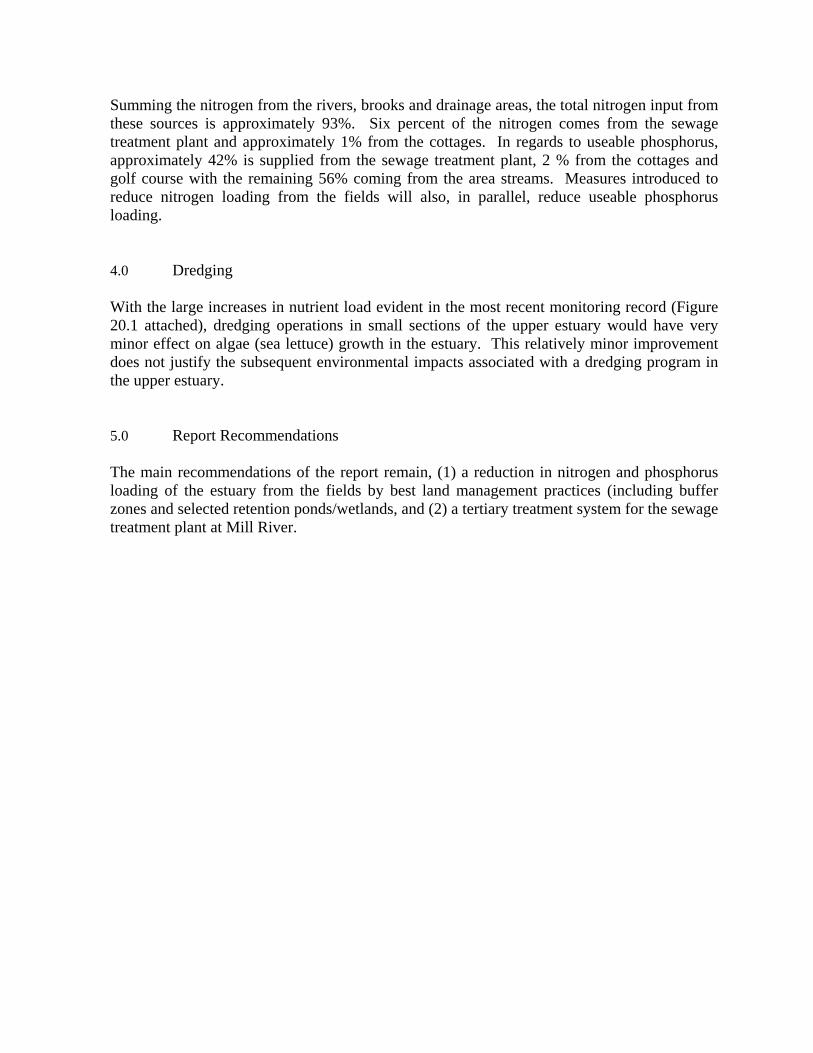
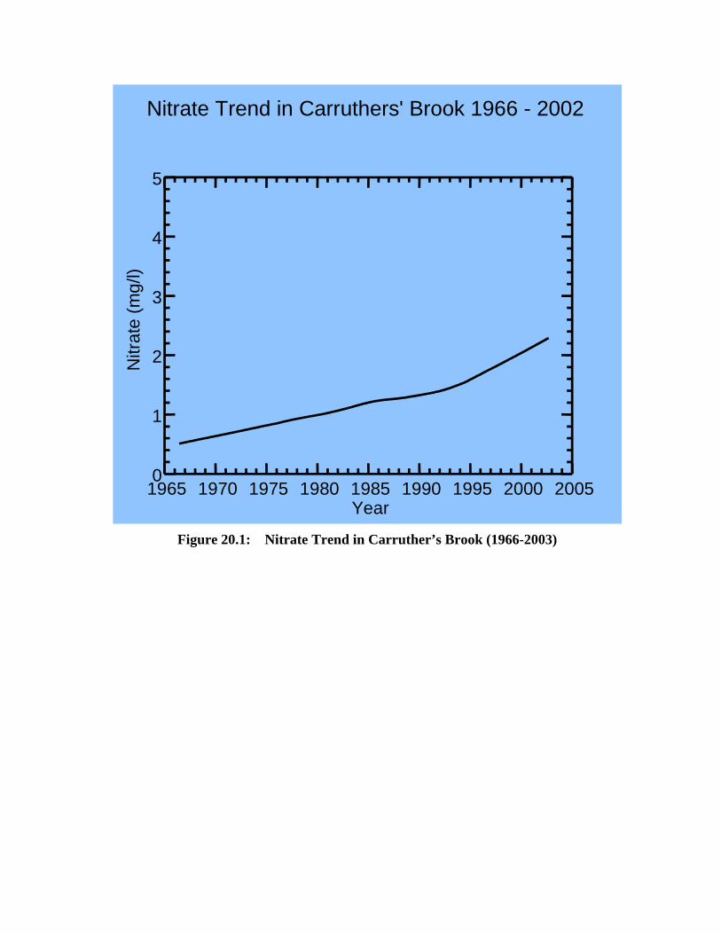
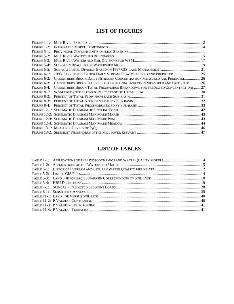
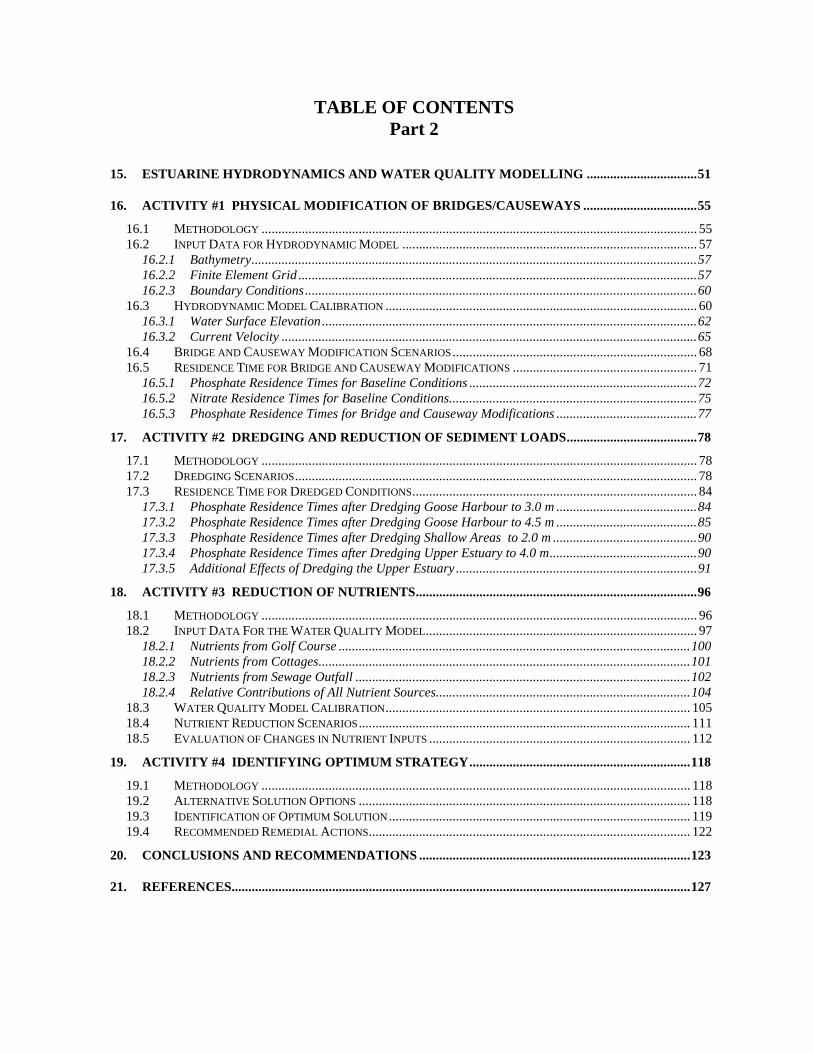
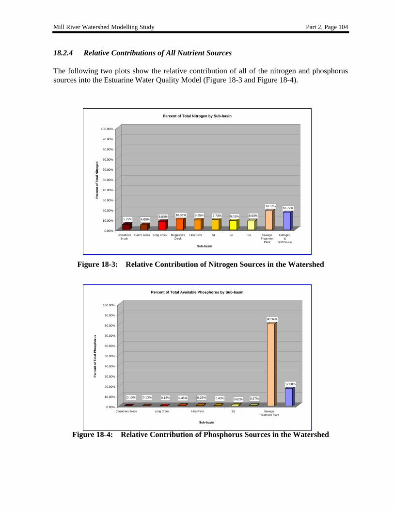
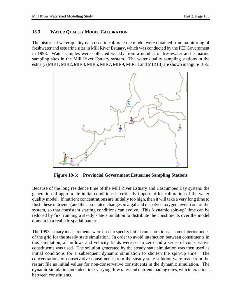
1.0 Data Update Subsequent to the submission of the final report, additional data has become available illustrating the increases in nitrate levels in Carruther’s Brook (the main fresh water input flow). The new data covers the years 1999 to 2002. These results are shown in attached Figure 20.1. Nitrate levels have increased significantly over the past 4 years. It can be seen that nitrate levels are now increasing at the rate of 6.7% per year. There has been a doubling of the nitrate load in Carruther’s Brook over the past 20 years. Since the hydrodynamic modelling has established that increased flushing of the estuary is not possible with physical modifications of the waterway (dredging, bridge widening, causeway opening), efforts should be directed to reducing watershed nitrate levels before they enter the estuary system. 2.0 Detention Ponds With such high increases in nutrient loading and expected parallel increases in sediment loading, in-stream detention ponds could fill rapidly, causing problems with fish life and migration in a short period of time. Commensurate with the philosophy of reducing nutrients and sediment loads before they enter streams, it would be better to incorporate detention ponds into some sections of the proposed and existing buffer zones. Ideally an effort would be made to naturalize the off-stream detention ponds and make them function more like wetlands, collecting sediment and removing nutrients. 3.0 Mislabelled Plot The ordinates in Figure 18.3 and 18.4 were mislabelled in the original report. The ordinate on the figures are percentage of nitrogen and phosphorus by concentration from the various sources. To see the impact of these concentrations factored by the volume flows from each input, the data is re-plotted in a new Figure 18.5 as percentage of total nutrients by mass supplied from each of the 10 identified sources. This figure clearly shows the relative contribution of each source in the watershed on nutrient loading in Mill River Estuary.

Summing the nitrogen from the rivers, brooks and drainage areas, the total nitrogen input from these sources is approximately 93%. Six percent of the nitrogen comes from the sewage treatment plant and approximately 1% from the cottages. In regards to useable phosphorus, approximately 42% is supplied from the sewage treatment plant, 2 % from the cottages and golf course with the remaining 56% coming from the area streams. Measures introduced to reduce nitrogen loading from the fields will also, in parallel, reduce useable phosphorus loading. 4.0 Dredging With the large increases in nutrient load evident in the most recent monitoring record (Figure 20.1 attached), dredging operations in small sections of the upper estuary would have very minor effect on algae (sea lettuce) growth in the estuary. This relatively minor improvement does not justify the subsequent environmental impacts associated with a dredging program in the upper estuary. 5.0 Report Recommendations The main recommendations of the report remain, (1) a reduction in nitrogen and phosphorus loading of the estuary from the fields by best land management practices (including buffer zones and selected retention ponds/wetlands, and (2) a tertiary treatment system for the sewage treatment plant at Mill River.

Relative Contributions From All Nutrient Sources

Car

ruth

ers

Broo

k

Cai

n's

Broo

k

Long

Cre

ek

Meg

giso

n's

Cre

ek

Hills

Riv

er

"S1"

"S2" "S3"

Sew

age

Trea

tmen

t Pla

nt

Cot

tage

s/G

olf C

ours

e

0

0.05

0.1

0.15

0.2

0.25

0.3

0.35

0.4

0.45

0.5

Sites

Perc

enta

ge A

mou

nt

Nitrogen Phosphorous

Figure 18.5: Relative Contribution of Nutrient Sources in the Watershed

1965 1970 1975 1980 1985 1990 1995 2000 2005Year

0

1

2

3

4

5

Nitr

ate

(mg/

l)Nitrate Trend in Carruthers' Brook 1966 - 2002

Figure 20.1: Nitrate Trend in Carruther’s Brook (1966-2003)

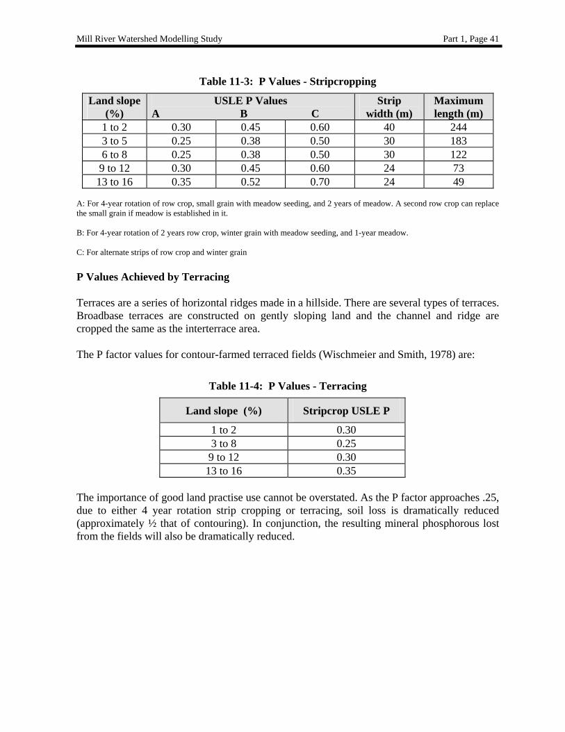
Executive Summary Observers of the Mill River Estuary (MRE) in Western PEI have noted deterioration in the health of the ecosystem during the last several decades. Algal blooms have increased in frequency and intensity, and instances of toxic algal blooms and oxygen depletion have been recorded. The growth and distribution of the seaweed “Sea Lettuce” (Ulva lactuca) has increased in the upper estuary and other sheltered coves since the mid-1980’s, causing loss of recreational and aesthetic value. These symptoms are indicators of eutrophication in the estuary. Eutrophic waterbodies are characterized by nutrient enrichment, and stimulation of rapid growth of algae and seaweeds before nutrients can be flushed from the ecosystem. In order to address the need for appropriate environmental management of the watershed and the estuary, the Mill River Watershed Roundtable (MRWRT) commissioned a modelling study. The goals of the study are to identify the multiple factors contributing to eutrophication of the MRE, to model the relative contributions of each, to recommend corrective measures for the factors, and to recommend an optimized solution to the eutrophication problem. Three separate baseline numerical studies were undertaken to a) model the surrounding Mill River watershed land usage (establishing nutrient and sediment loadings via runoff), b) model the estuary hydrodynamics and c) model estuary water quality. These models were calibrated to match 1993 field measurements (the most recent comprehensive set available) and ‘mimic’ the present system overall. At this point, potential remedial measures were then applied to see their effects to the system. These remedial measures examined include: ! Physical changes to the Cascumpec bridge and causeway dimensions; ! Changes to the MRE channel and harbour entrance dimensions (i.e. dredging); ! Effects of nutrient reduction from agricultural runoffs due to combination of better land

management practises and construction of man-made marshes/settling ponds; ! Improvement to the Rodd Mill River Resort sewage treatment plant and; ! Golf course/cottage septic field improvements.

The models indicate that the neither the dredging of the outer channels or harbour entrances, or modifications to bridges/causeways will have a significant positive effective in reducing the eutrophication problem. The optimum long-term strategy for reduction of eutrophication in the Mill River Estuary involves the following components: ! Reducing nutrient inputs from the surrounding watershed areas to 75% of the 1993

modelled values using a combination of: (a) using best management practices for agricultural land; and (b) creation of man made wetlands and/or settling ponds in the major estuary tributaries to reduce nutrient and sedimentation loading;

! Converting the resort treatment plant into a tertiary treatment facility, resulting in up to an 80% improvement in plant outfall nutrient reduction;

! Dredging of the upper estuary region to increase water depth to inhibit growth of bottom attached Ulva.

TABLE OF CONTENTS Part 1

EXECUTIVE SUMMARY................................................................................................................................... I

1. INTRODUCTION .......................................................................................................................................1

1.1 BACKGROUND OF THE STUDY.................................................................................................................... 1 1.2 STUDY OBJECTIVES ................................................................................................................................... 1 1.3 SCOPE OF WORK ........................................................................................................................................ 3 1.4 MODELLING APPROACH............................................................................................................................. 3 1.5 ORGANIZATION OF THE REPORT ................................................................................................................ 5

2. INTRODUCTION TO WATERSHED MODELLING ...........................................................................6

3. THE MILL RIVER ESTUARY WATERSHED MODEL ......................................................................7

3.1 OVERALL METHODOLOGY......................................................................................................................... 7

4. DEFINITION OF TERMS .........................................................................................................................8

5. WATERSHED MODEL INPUT FILES ..................................................................................................9

5.1 DETERMINATION OF DATA AVAILABILITY................................................................................................. 9 5.1.1 Data Selection for Calibration of Flow and Water Quality ............................................................9 5.1.2 Weather Data ................................................................................................................................13 5.1.3 General Data Availability for WSM Input Files............................................................................13

5.2 USE OF THE PEI GEOGRAPHICAL INFORMATION SYSTEM ........................................................................ 13 5.2.1 Land Use Data Availability ...........................................................................................................13 5.2.2 Watershed Definition.....................................................................................................................14 5.2.3 HRU Definition..............................................................................................................................15

5.3 SOILS ....................................................................................................................................................... 15 5.3.1 Prince Edward Island Soils ...........................................................................................................15

5.4 LAND USE BY AREA FOR WSM HRU INPUT FILE DEFINITION ................................................................ 17 5.5 SUBBASIN AND HYDROLOGICAL RESPONSE UNITS (HRU) ...................................................................... 18 5.6 REACH DEFINITION.................................................................................................................................. 19 5.7 LAND MANAGEMENT DEFINITION FOR THE WSM ................................................................................... 20 5.8 GROUNDWATER ....................................................................................................................................... 20

6. CALIBRATION OF WSM TO KNOWN CONDITIONS.....................................................................22

6.1 STREAM FLOW CALIBRATION .................................................................................................................. 22 6.2 NITROGEN AND PHOSPHOROUS CALIBRATION ......................................................................................... 23

7. SEDIMENT LOADING FROM WATERSHED AREAS .....................................................................28

8. RESULTS ...................................................................................................................................................29

8.1 SENSITIVITY ANALYSIS FOR WSM RESULTS ........................................................................................... 34

9. DISCUSSION OF MILL RIVER WATERSHED MODEL RESULTS...............................................36

10. THE POTENTIAL OF WATERSHED MODELLING.........................................................................38

11. SOIL LOSS AND SEDIMENTATION BASED ON LAND USAGE ...................................................39

12. CONSTRUCTED WETLANDS AND SETTLING PONDS .................................................................42

13. POTENTIAL OF MILL RIVER SEDIMENT AS A FUTURE NUTRIENT SOURCE.....................45

13.1 HISTORICAL PHOSPHORUS IN AGRICULTURAL SOIL ............................................................................ 45 13.2 MILL RIVER SEDIMENT SAMPLES........................................................................................................ 47 13.3 DISCUSSION ........................................................................................................................................ 48

14. REFERENCES ..........................................................................................................................................50

LIST OF FIGURES

FIGURE 1-1: MILL RIVER ESTUARY ...................................................................................................................... 2 FIGURE 1-2: INTEGRATED MODEL COMPONENTS.................................................................................................. 4 FIGURE 5-1: PROVINCIAL GOVERNMENT SAMPLING STATIONS .......................................................................... 11 FIGURE 5-2: MILL RIVER WATERSHED BOUNDARIES.......................................................................................... 15 FIGURE 5-3: MILL RIVER WATERSHED SOIL DIVISIONS FOR WSM..................................................................... 17 FIGURE 5-4: SUB-BASIN REACHES FOR WATERSHED MODEL.............................................................................. 19 FIGURE 5-5: SUB-WATERSHED DIVISION BASED ON 1997 GIS LAND MANAGEMENT......................................... 21 FIGURE 6-1: 1993 CARRUTHERS BROOK DAILY STREAM FLOW MEASURED AND PREDICTED ............................ 25 FIGURE 6-2: CARRUTHERS BROOK DAILY NITROGEN CONCENTRATION MEASURED AND PREDICTED................ 26 FIGURE 6-3: CARRUTHERS BROOK DAILY PHOSPHORUS CONCENTRATION MEASURED AND PREDICTED ........... 26 FIGURE 6-4: CARRUTHERS BROOK TOTAL PHOSPHORUS BREAKDOWN FOR PREDICTED CONCENTRATIONS....... 27 FIGURE 8-1: WSM PREDICTED FLOWS & PERCENTAGE OF TOTAL FLOW........................................................... 30 FIGURE 8-2: PERCENT OF TOTAL FLOW FROM EACH SUB-BASIN ......................................................................... 31 FIGURE 8-3: PERCENT OF TOTAL NITROGEN LOAD BY SUB-BASIN...................................................................... 32 FIGURE 8-4: PERCENT OF TOTAL PHOSPHORUS LOAD BY SUB-BASIN ................................................................. 33 FIGURE 12-1: SCHEMATIC DIAGRAM OF SETTLING POND ..................................................................................... 42 FIGURE 12-2: SCHEMATIC DIAGRAM MAN MADE MARSH.................................................................................... 43 FIGURE 12-3: SCHEMATIC DIAGRAM MAN MADE POND....................................................................................... 43 FIGURE 12-4: SCHEMATIC DIAGRAM MAN MADE MEADOW................................................................................. 44 FIGURE 13-1: MEASURED LEVELS OF P2O5 ........................................................................................................... 46 FIGURE 13-2: SEDIMENT PHOSPHORUS IN THE MILL RIVER ESTUARY .................................................................. 47

LIST OF TABLES

TABLE 1-1: APPLICATIONS OF THE HYDRODYNAMICS AND WATER QUALITY MODELS ........................................ 4 TABLE 1-2: APPLICATIONS OF THE WATERSHED MODEL ...................................................................................... 5 TABLE 5-1: HISTORICAL STREAM AND ESTUARY WATER QUALITY FIELD DATA ............................................... 12 TABLE 5-2: LIST OF GIS FILES............................................................................................................................ 14 TABLE 5-3: LAND USE FOR EACH SUB-BASIN CORRESPONDING TO SOIL TYPE ................................................... 18 TABLE 5-4: HRU DEFINITIONS ........................................................................................................................... 19 TABLE 7-1: SUB-BASIN PREDICTED SEDIMENT LOADS........................................................................................ 28 TABLE 8-1: SENSITIVITY ANALYSIS .................................................................................................................... 35 TABLE 11-1: LAND USE VERSUS SOIL LOSS ......................................................................................................... 40 TABLE 11-2: P VALUES - CONTOURING................................................................................................................ 40 TABLE 11-3: P VALUES - STRIPCROPPING............................................................................................................. 41 TABLE 11-4: P VALUES - TERRACING................................................................................................................... 41

TABLE OF CONTENTS Part 2

15. ESTUARINE HYDRODYNAMICS AND WATER QUALITY MODELLING .................................51

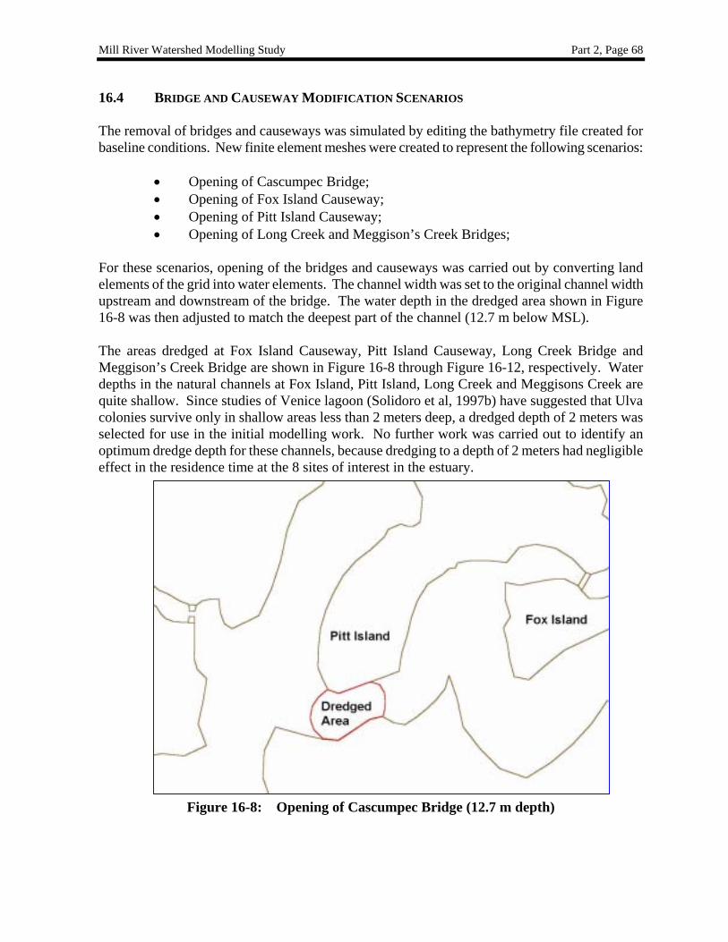
16. ACTIVITY #1 PHYSICAL MODIFICATION OF BRIDGES/CAUSEWAYS ..................................55

16.1 METHODOLOGY .................................................................................................................................. 55 16.2 INPUT DATA FOR HYDRODYNAMIC MODEL ........................................................................................ 57

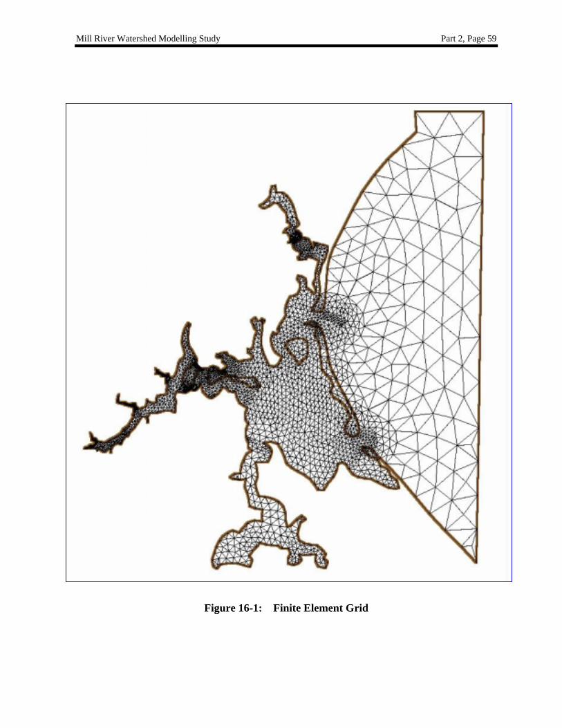
16.2.1 Bathymetry.....................................................................................................................................57 16.2.2 Finite Element Grid .......................................................................................................................57 16.2.3 Boundary Conditions.....................................................................................................................60

16.3 HYDRODYNAMIC MODEL CALIBRATION ............................................................................................. 60 16.3.1 Water Surface Elevation ................................................................................................................62 16.3.2 Current Velocity ............................................................................................................................65

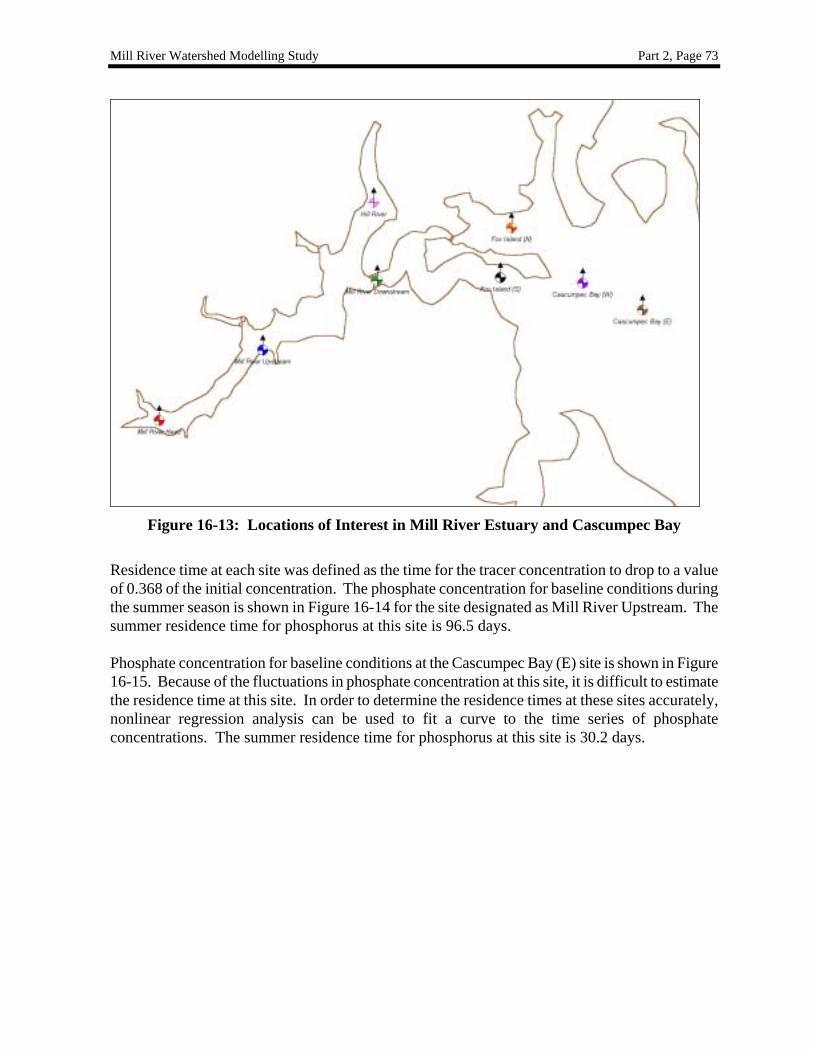
16.4 BRIDGE AND CAUSEWAY MODIFICATION SCENARIOS......................................................................... 68 16.5 RESIDENCE TIME FOR BRIDGE AND CAUSEWAY MODIFICATIONS ....................................................... 71

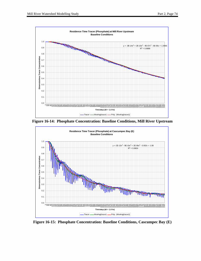
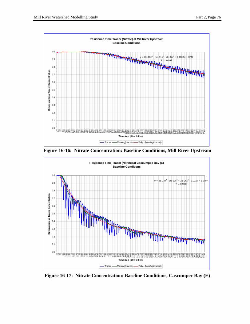
16.5.1 Phosphate Residence Times for Baseline Conditions ....................................................................72 16.5.2 Nitrate Residence Times for Baseline Conditions..........................................................................75 16.5.3 Phosphate Residence Times for Bridge and Causeway Modifications ..........................................77

17. ACTIVITY #2 DREDGING AND REDUCTION OF SEDIMENT LOADS.......................................78

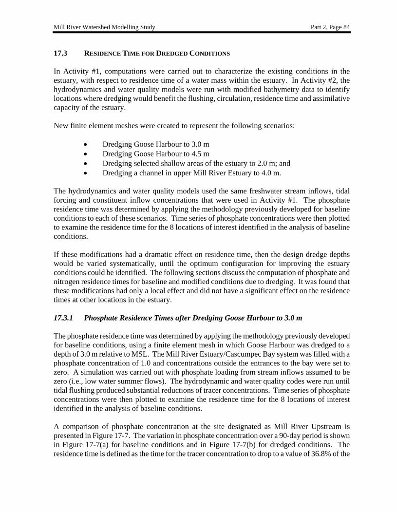
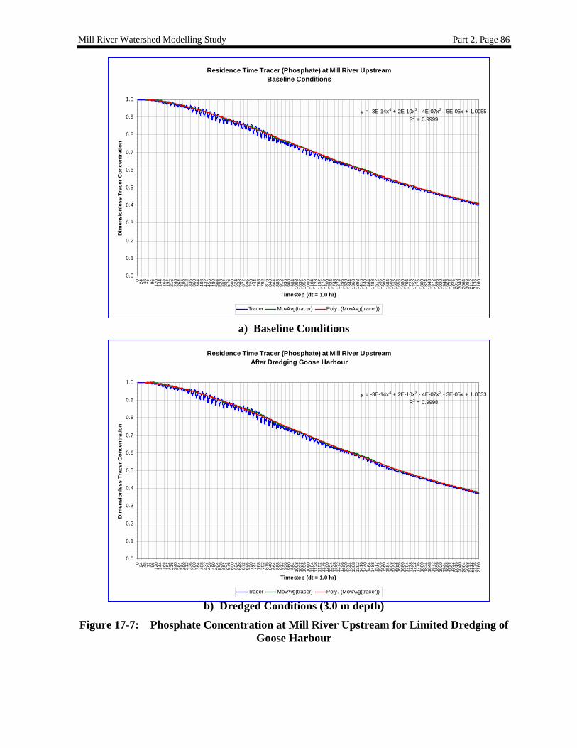
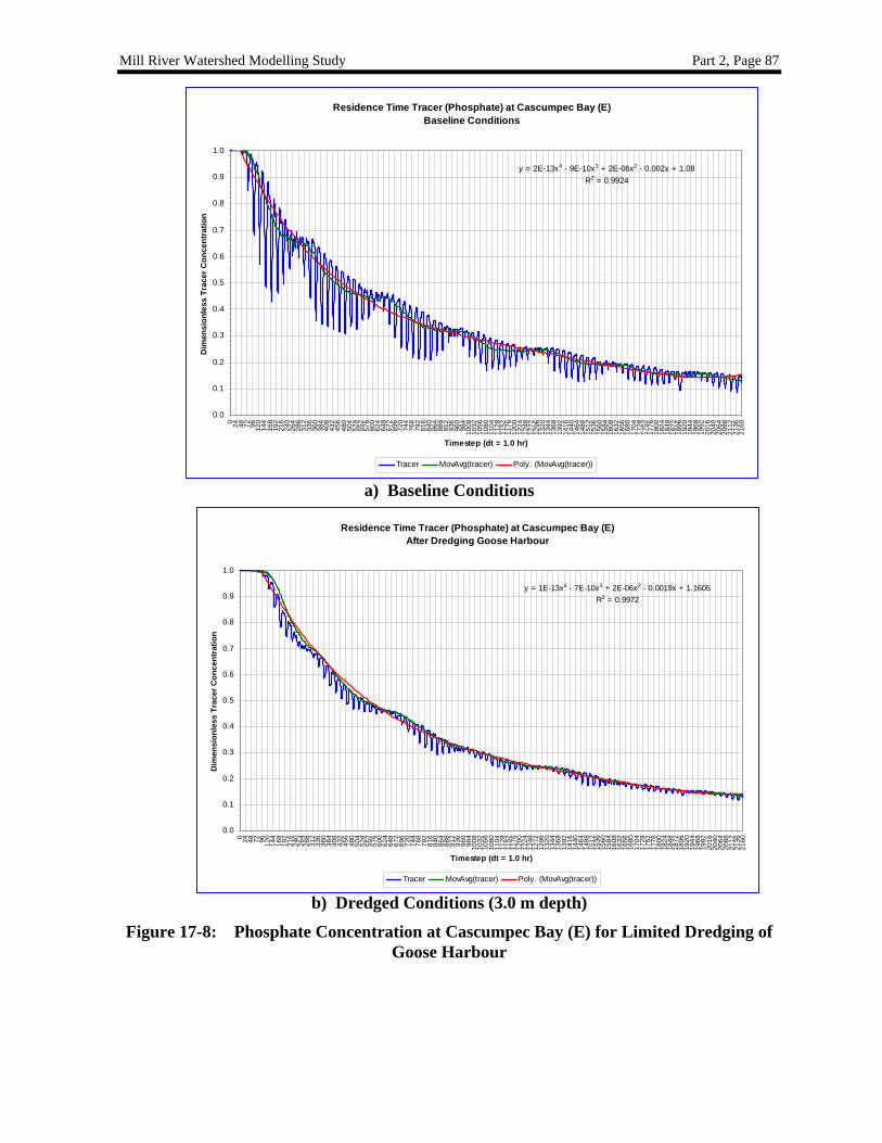
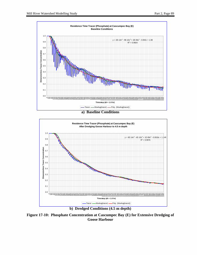
17.1 METHODOLOGY .................................................................................................................................. 78 17.2 DREDGING SCENARIOS........................................................................................................................ 78 17.3 RESIDENCE TIME FOR DREDGED CONDITIONS..................................................................................... 84

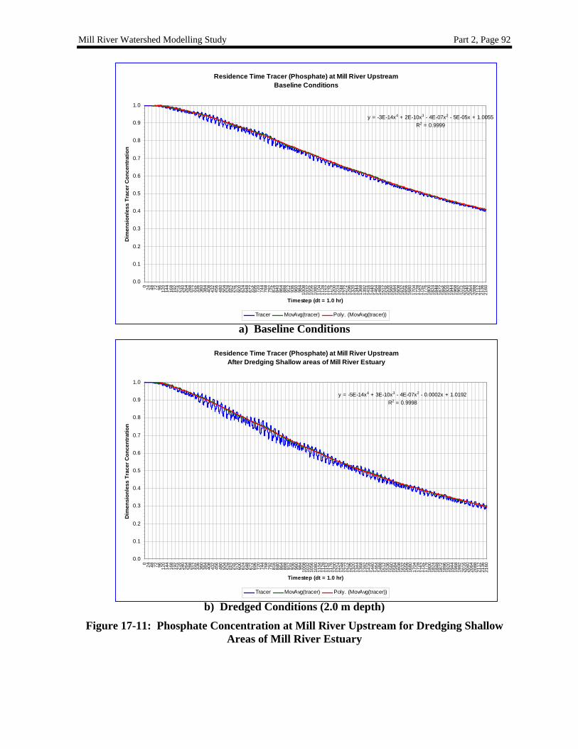
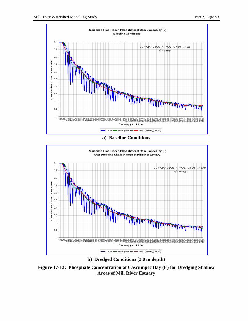
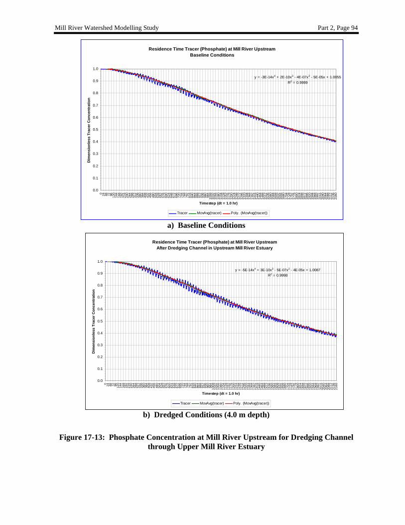
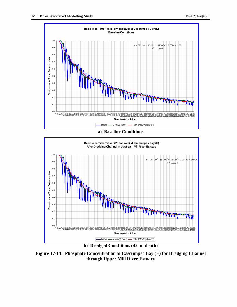
17.3.1 Phosphate Residence Times after Dredging Goose Harbour to 3.0 m ..........................................84 17.3.2 Phosphate Residence Times after Dredging Goose Harbour to 4.5 m ..........................................85 17.3.3 Phosphate Residence Times after Dredging Shallow Areas to 2.0 m ...........................................90 17.3.4 Phosphate Residence Times after Dredging Upper Estuary to 4.0 m............................................90 17.3.5 Additional Effects of Dredging the Upper Estuary ........................................................................91

18. ACTIVITY #3 REDUCTION OF NUTRIENTS....................................................................................96

18.1 METHODOLOGY .................................................................................................................................. 96 18.2 INPUT DATA FOR THE WATER QUALITY MODEL................................................................................. 97

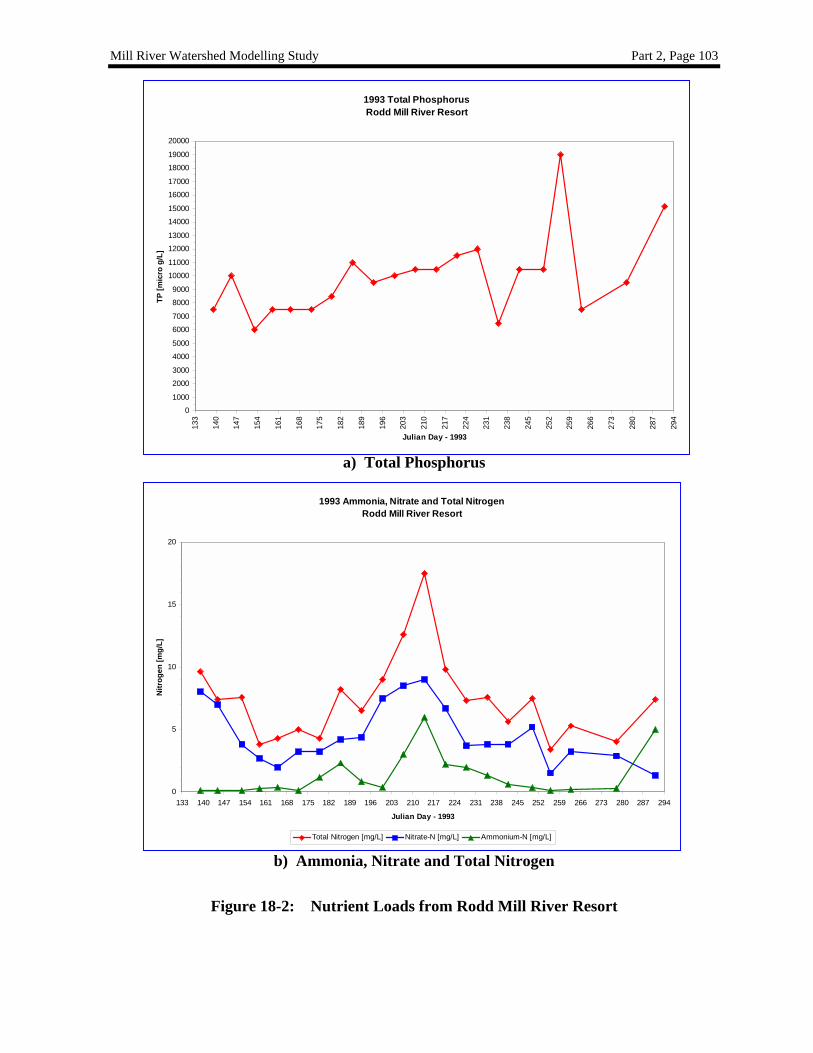
18.2.1 Nutrients from Golf Course .........................................................................................................100 18.2.2 Nutrients from Cottages...............................................................................................................101 18.2.3 Nutrients from Sewage Outfall ....................................................................................................102 18.2.4 Relative Contributions of All Nutrient Sources............................................................................104

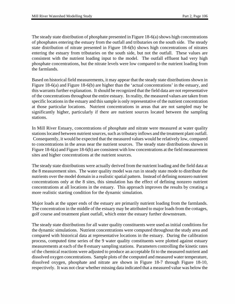
18.3 WATER QUALITY MODEL CALIBRATION........................................................................................... 105 18.4 NUTRIENT REDUCTION SCENARIOS................................................................................................... 111 18.5 EVALUATION OF CHANGES IN NUTRIENT INPUTS .............................................................................. 112

19. ACTIVITY #4 IDENTIFYING OPTIMUM STRATEGY..................................................................118

19.1 METHODOLOGY ................................................................................................................................ 118 19.2 ALTERNATIVE SOLUTION OPTIONS ................................................................................................... 118 19.3 IDENTIFICATION OF OPTIMUM SOLUTION.......................................................................................... 119 19.4 RECOMMENDED REMEDIAL ACTIONS................................................................................................ 122

20. CONCLUSIONS AND RECOMMENDATIONS .................................................................................123

21. REFERENCES.........................................................................................................................................127

TABLE OF CONTENTS CONTINUED Part 2

APPENDIX A - SUPPORT ACKNOWLEGEMENT

APPENDIX B - SOIL CHARACTERISTICS

APPENDIX C - LAND TOPOLOGY

APPENDIX D - LAND MANAGEMENT - GENERAL

APPENDIX E - CROP CHARACTERISTICS

APPENDIX F - LAND MANAGEMENT FERTILIZER

APPENDIX G - HARVEST AND KILL OPERATIONS

APPENDIX H - GROUNDWATER SPECIFICATION

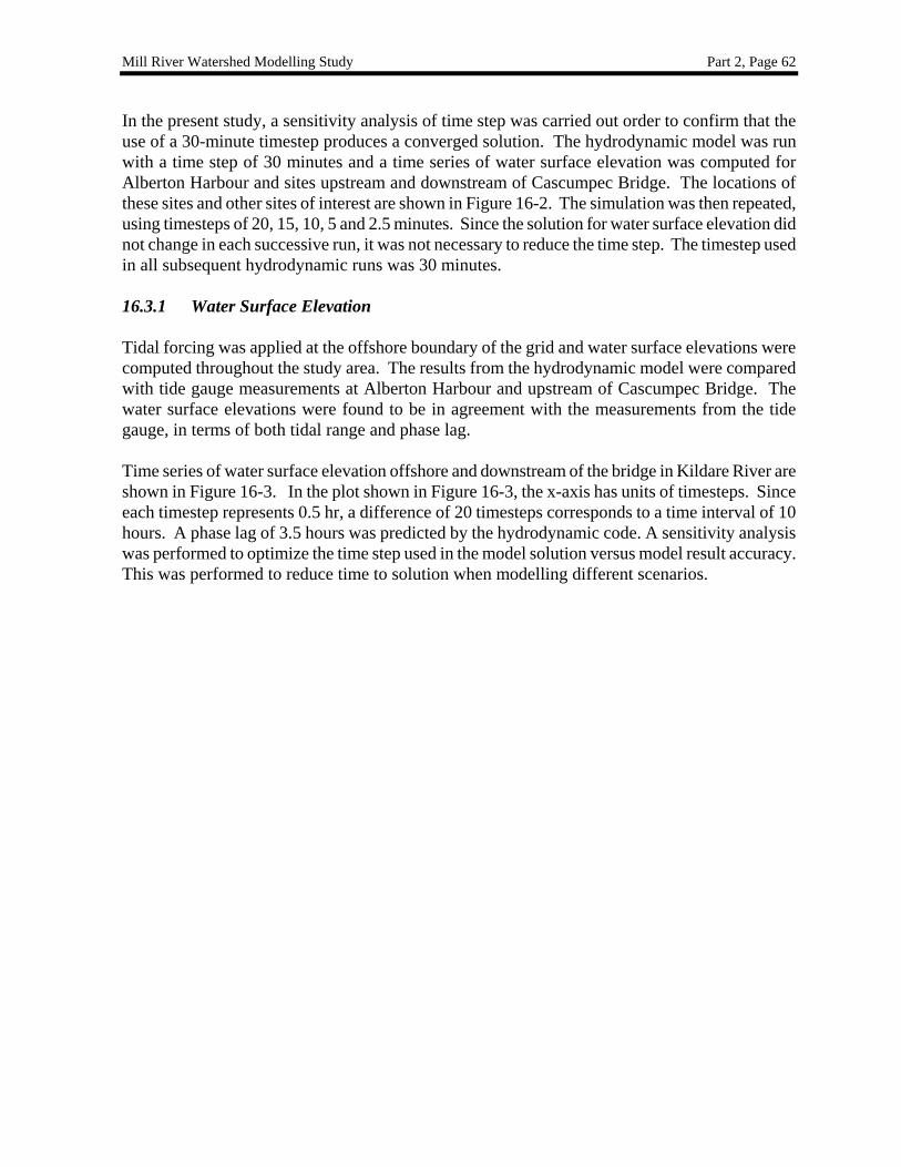
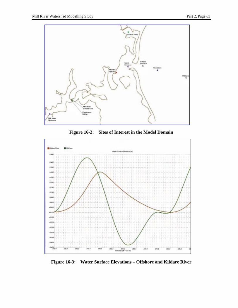
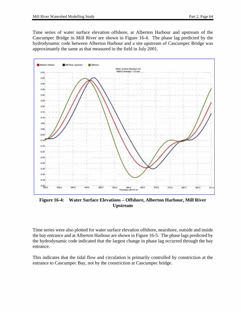
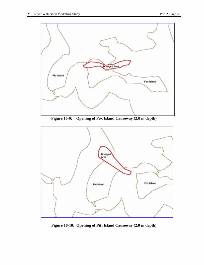
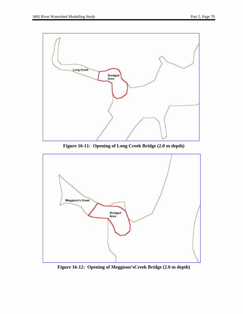
LIST OF FIGURES FIGURE 16-1: FINITE ELEMENT GRID .................................................................................................................. 59 FIGURE 16-2: SITES OF INTEREST IN THE MODEL DOMAIN.................................................................................. 63 FIGURE 16-3: WATER SURFACE ELEVATIONS – OFFSHORE AND KILDARE RIVER ............................................... 63 FIGURE 16-4: WATER SURFACE ELEVATIONS – OFFSHORE, ALBERTON HARBOUR, MILL RIVER UPSTREAM..... 64 FIGURE 16-5: WATER SURFACE ELEVATIONS – OFFSHORE, NEARSHORE, OUTSIDE ENTRANCE, INSIDE ENTRANCE

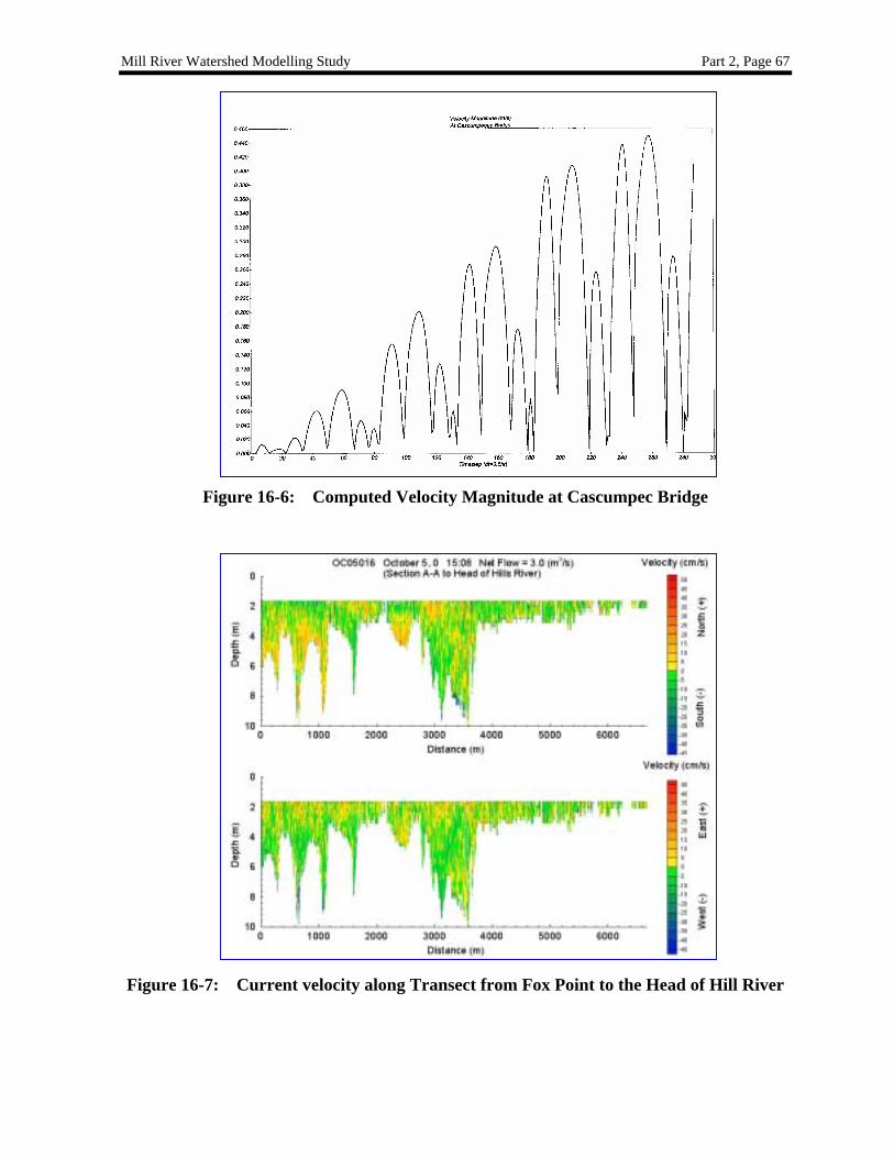
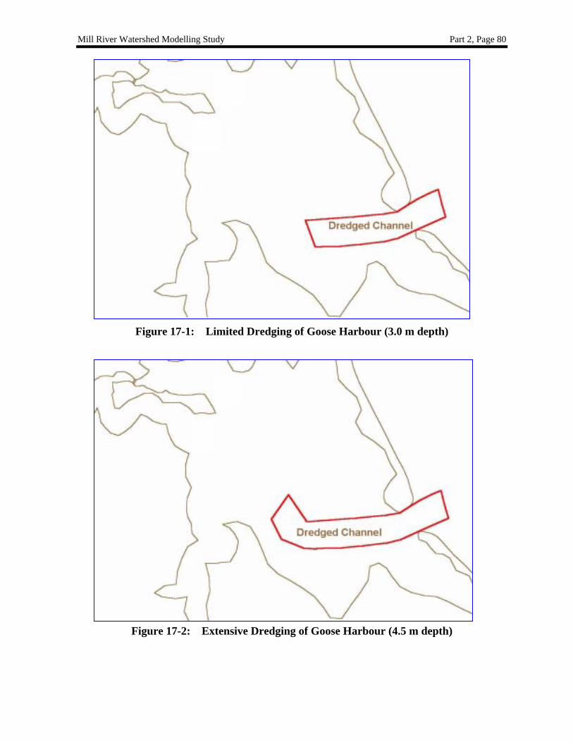
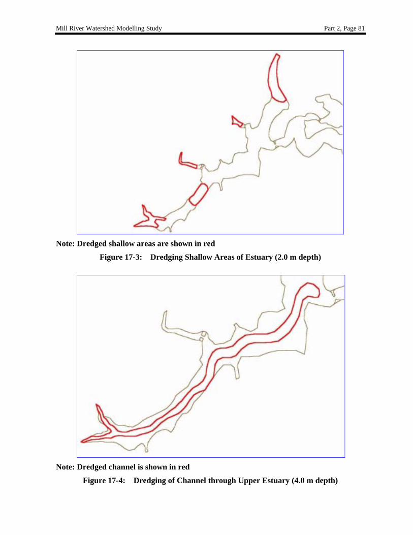
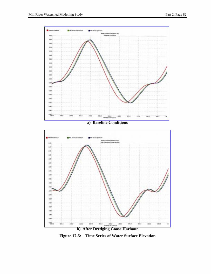
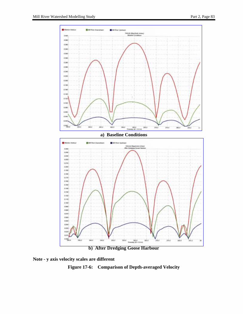
AND ALBERTON HARBOUR ............................................................................................................ 65 FIGURE 16-6: COMPUTED VELOCITY MAGNITUDE AT CASCUMPEC BRIDGE ....................................................... 67 FIGURE 16-7: CURRENT VELOCITY ALONG TRANSECT FROM FOX POINT TO THE HEAD OF HILL RIVER .............. 67 FIGURE 16-8: OPENING OF CASCUMPEC BRIDGE (12.7 M DEPTH)........................................................................ 68 FIGURE 16-9: OPENING OF FOX ISLAND CAUSEWAY (2.0 M DEPTH).................................................................... 69 FIGURE 16-10: OPENING OF PITT ISLAND CAUSEWAY (2.0 M DEPTH).................................................................... 69 FIGURE 16-11: OPENING OF LONG CREEK BRIDGE (2.0 M DEPTH) ........................................................................ 70 FIGURE 16-12: OPENING OF MEGGISON’SCREEK BRIDGE (2.0 M DEPTH) .............................................................. 70 FIGURE 16-13: LOCATIONS OF INTEREST IN MILL RIVER ESTUARY AND CASCUMPEC BAY .................................. 73 FIGURE 16-14: PHOSPHATE CONCENTRATION: BASELINE CONDITIONS, MILL RIVER UPSTREAM......................... 74 FIGURE 16-15: PHOSPHATE CONCENTRATION: BASELINE CONDITIONS, CASCUMPEC BAY (E)............................. 74 FIGURE 16-16: NITRATE CONCENTRATION: BASELINE CONDITIONS, MILL RIVER UPSTREAM.............................. 76 FIGURE 16-17: NITRATE CONCENTRATION: BASELINE CONDITIONS, CASCUMPEC BAY (E) ................................. 76 FIGURE 17-1: LIMITED DREDGING OF GOOSE HARBOUR (3.0 M DEPTH).............................................................. 80 FIGURE 17-2: EXTENSIVE DREDGING OF GOOSE HARBOUR (4.5 M DEPTH) ......................................................... 80 FIGURE 17-3: DREDGING SHALLOW AREAS OF ESTUARY (2.0 M DEPTH) ............................................................ 81 FIGURE 17-4: DREDGING OF CHANNEL THROUGH UPPER ESTUARY (4.0 M DEPTH) ............................................. 81 FIGURE 17-5: TIME SERIES OF WATER SURFACE ELEVATION ............................................................................. 82 FIGURE 17-6: COMPARISON OF DEPTH-AVERAGED VELOCITY ............................................................................ 83 FIGURE 17-7: PHOSPHATE CONCENTRATION AT MILL RIVER UPSTREAM FOR LIMITED DREDGING OF GOOSE

HARBOUR ...................................................................................................................................... 86 FIGURE 17-8: PHOSPHATE CONCENTRATION AT CASCUMPEC BAY (E) FOR LIMITED DREDGING OF GOOSE

HARBOUR ...................................................................................................................................... 87 FIGURE 17-9: PHOSPHATE CONCENTRATION AT MILL RIVER UPSTREAM FOR EXTENSIVE DREDGING OF GOOSE

HARBOUR ...................................................................................................................................... 88 FIGURE 17-10: PHOSPHATE CONCENTRATION AT CASCUMPEC BAY (E) FOR EXTENSIVE DREDGING OF GOOSE

HARBOUR ...................................................................................................................................... 89 FIGURE 17-11: PHOSPHATE CONCENTRATION AT MILL RIVER UPSTREAM FOR DREDGING SHALLOW AREAS OF

MILL RIVER ESTUARY ................................................................................................................... 92 FIGURE 17-12: PHOSPHATE CONCENTRATION AT CASCUMPEC BAY (E) FOR DREDGING SHALLOW AREAS OF MILL

RIVER ESTUARY ............................................................................................................................ 93 FIGURE 17-13: PHOSPHATE CONCENTRATION AT MILL RIVER UPSTREAM FOR DREDGING CHANNEL THROUGH

UPPER MILL RIVER ESTUARY ........................................................................................................ 94 FIGURE 17-14: PHOSPHATE CONCENTRATION AT CASCUMPEC BAY (E) FOR DREDGING CHANNEL THROUGH UPPER

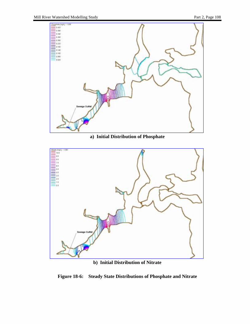
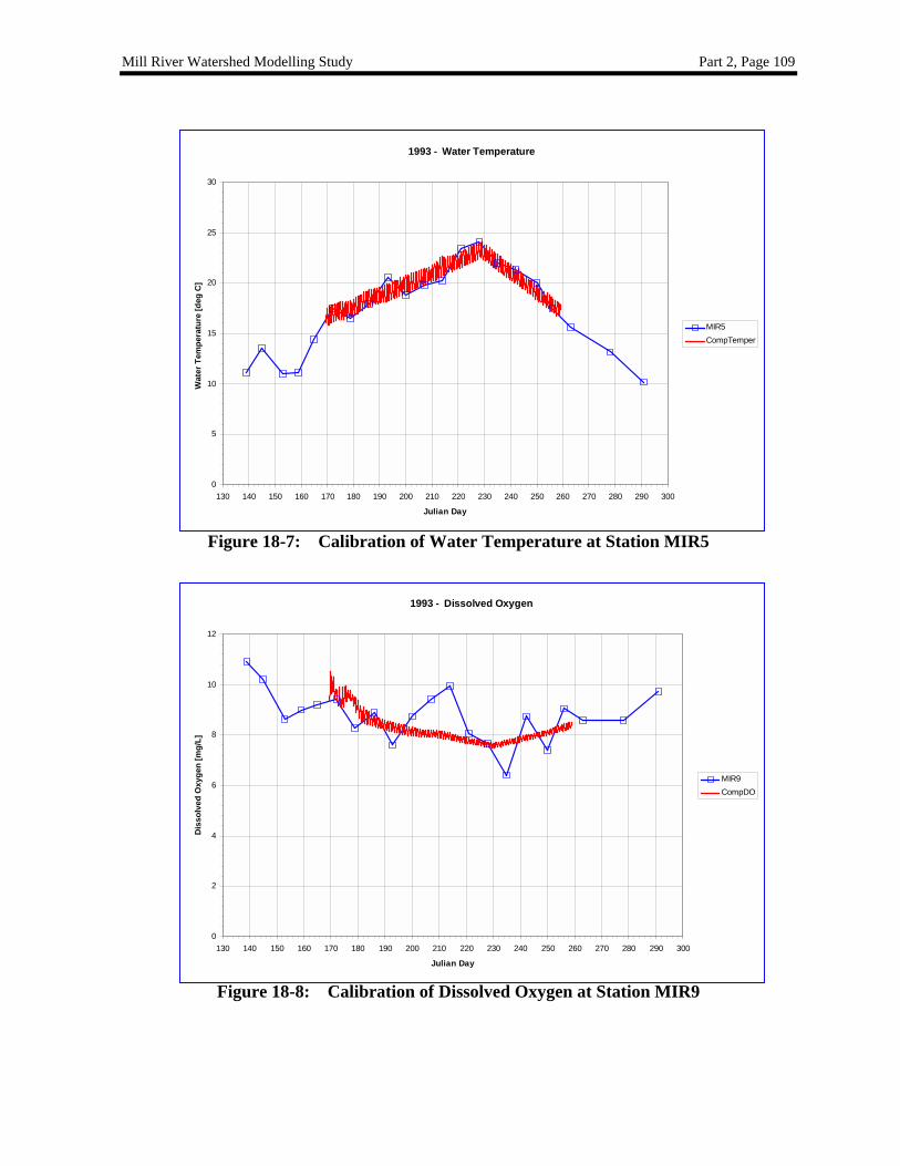
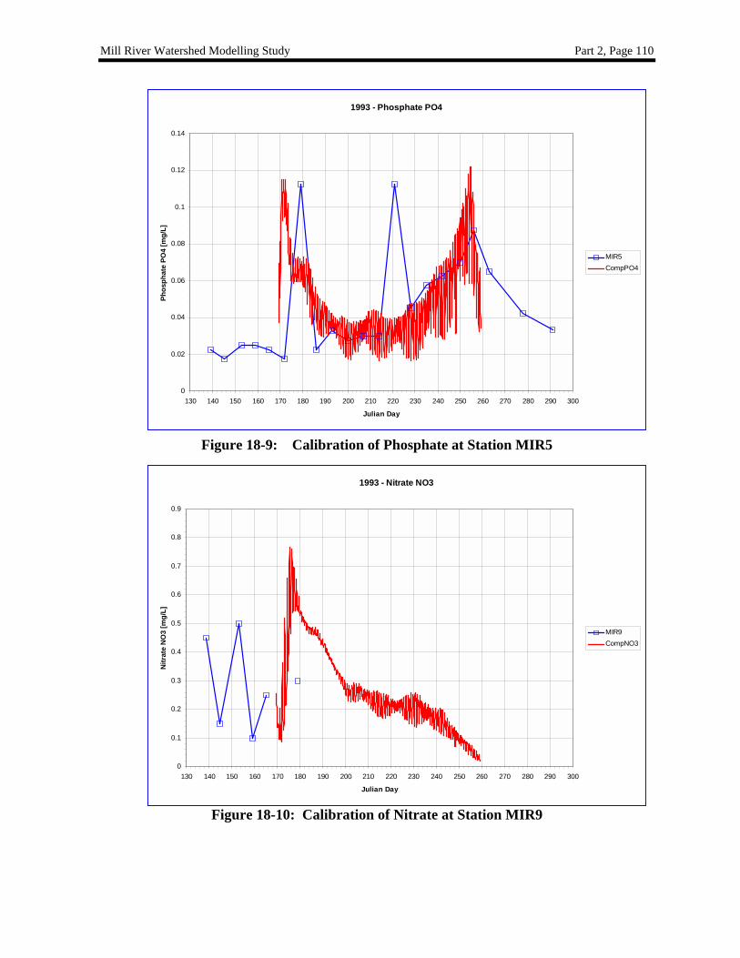
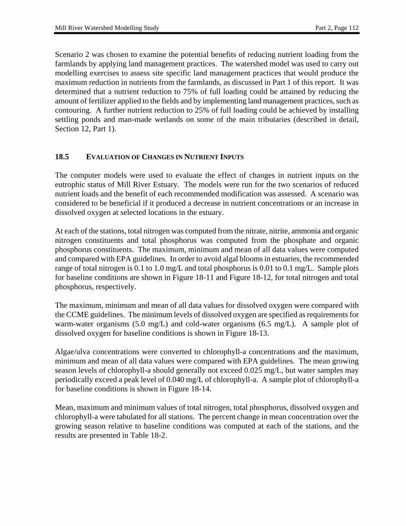
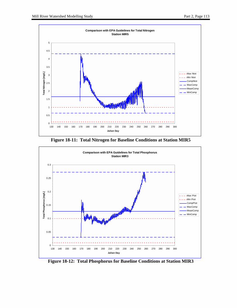
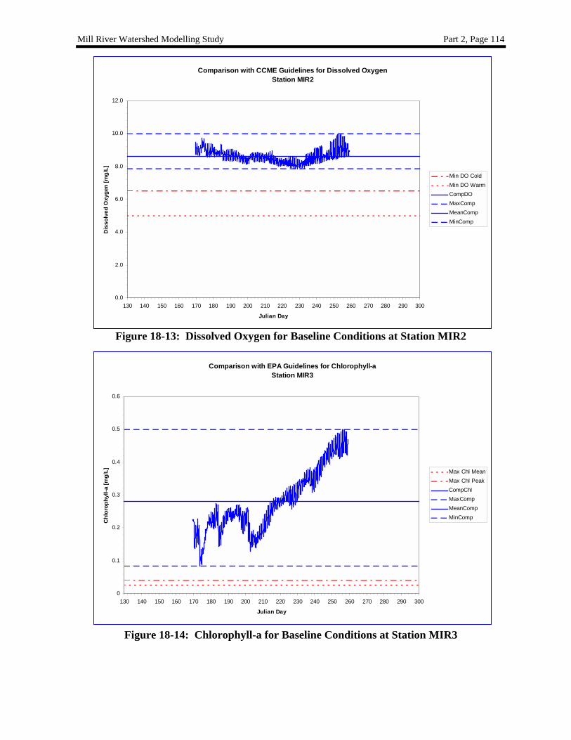
MILL RIVER ESTUARY ................................................................................................................... 95 FIGURE 18-1: LOCATION OF TRIBUTARIES AND SEWAGE OUTFALL..................................................................... 99 FIGURE 18-2: NUTRIENT LOADS FROM RODD MILL RIVER RESORT .................................................................. 103 FIGURE 18-3: RELATIVE CONTRIBUTION OF NITROGEN SOURCES IN THE WATERSHED..................................... 104 FIGURE 18-4: RELATIVE CONTRIBUTION OF PHOSPHORUS SOURCES IN THE WATERSHED ................................ 104 FIGURE 18-5: PROVINCIAL GOVERNMENT ESTUARINE SAMPLING STATIONS.................................................... 105 FIGURE 18-6: STEADY STATE DISTRIBUTIONS OF PHOSPHATE AND NITRATE.................................................... 108 FIGURE 18-7: CALIBRATION OF WATER TEMPERATURE AT STATION MIR5...................................................... 109 FIGURE 18-8: CALIBRATION OF DISSOLVED OXYGEN AT STATION MIR9 ......................................................... 109 FIGURE 18-9: CALIBRATION OF PHOSPHATE AT STATION MIR5 ....................................................................... 110 FIGURE 18-10: CALIBRATION OF NITRATE AT STATION MIR9 ............................................................................ 110 FIGURE 18-11: TOTAL NITROGEN FOR BASELINE CONDITIONS AT STATION MIR5 ............................................. 113 FIGURE 18-12: TOTAL PHOSPHORUS FOR BASELINE CONDITIONS AT STATION MIR3......................................... 113 FIGURE 18-13: DISSOLVED OXYGEN FOR BASELINE CONDITIONS AT STATION MIR2......................................... 114

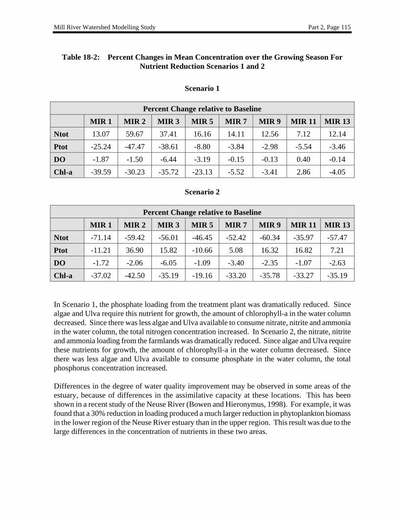
FIGURE 18-14: CHLOROPHYLL-A FOR BASELINE CONDITIONS AT STATION MIR3 .............................................. 114

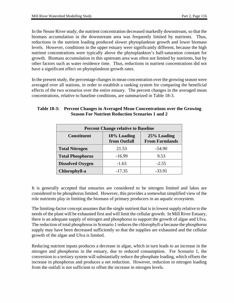
LIST OF TABLES TABLE 18-1: TYPICAL TN AND TP IN TREATMENT PLANT EFFLUENT............................................................... 111 TABLE 18-2: PERCENT CHANGES IN MEAN CONCENTRATION OVER THE GROWING SEASON FOR NUTRIENT

REDUCTION SCENARIOS 1 AND 2 ................................................................................................. 115 TABLE 18-3: PERCENT CHANGES IN AVERAGED MEAN CONCENTRATIONS OVER THE GROWING SEASON FOR

NUTRIENT REDUCTION SCENARIOS 1 AND 2 ................................................................................ 116 TABLE 19-1: PERCENT CHANGES IN AVERAGED MEAN CONCENTRATIONS OVER THE GROWING SEASON FOR

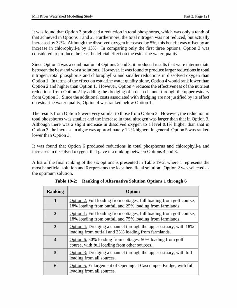
ALTERNATIVE SOLUTION OPTIONS 1 THROUGH 6 ........................................................................ 120 TABLE 19-2: RANKING OF ALTERNATIVE SOLUTION OPTIONS 1 THROUGH 6.................................................... 121


Part 1: Watershed Modelling

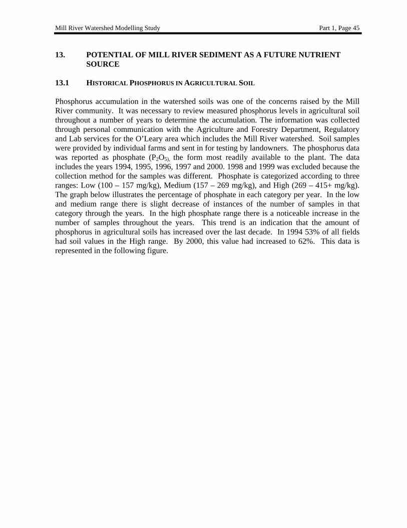
Mill River Watershed Modelling Study Part 1, Page 1

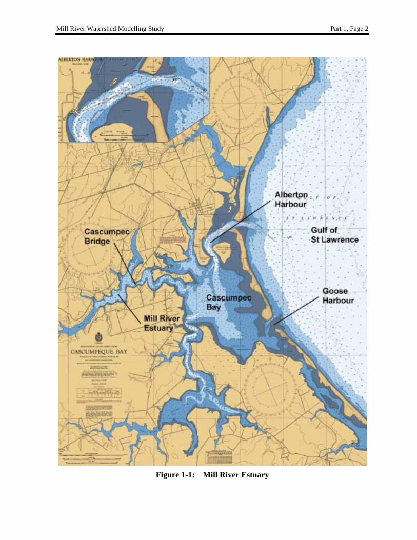
1. INTRODUCTION 1.1 BACKGROUND OF THE STUDY The Mill River estuary extends approximately 8.75 km from Bloomfield Corner to Cascumpec Bridge, where it discharges into Cascumpec Bay and, ultimately, into the Gulf of St. Lawrence (see Figure 1-1). Cascumpec Bay is a typical PEI north shore embayment, partially separated from the Gulf of St. Lawrence by a barrier dune island system, with entrances at Alberton and (the now mostly infilled) Goose Harbour. The Mill River Golf Course and Resort, the Mill River Provincial Park and Fun Park lie at the head of the estuary. There are numerous seasonal cottages along the shores of the estuary, particularly the eastern side, and numerous permanent homes in the vicinity. The watershed area is approximately 137 sq. km, with 50% forested, 47% agricultural use (about equally distributed among potatoes, grain and hay), and the remainder of mixed use. Since the mid-1980’s, an increase in sea lettuce has been noted in the upper estuary and other sheltered coves. The presence of sea lettuce has been directly attributed to severe eutrophication of much of the estuary. Decay of these marine plants has resulted in extensive areas of low oxygen in the sediments and bottom waters, with odours of sulphide and decaying vegetation. Nutrients (phosphorus and nitrogen) contributing to the growth of sea lettuce have several sources, including excess soil-nutrient loss from farmlands, treated effluent from the Mill River resort and golf course, and septic fields of the numerous shoreline cottages. Some local residents believe that long-term sedimentation and the construction of bridges and causeways across several of the natural channels have reduced the assimilative capacity of the estuary, by altering the water circulation, flushing, residence time and water mass exchange. The Mill River Watershed Roundtable was formed from a local community group (the Mill River Watershed Improvement Committee) and relevant government departments in Prince Edward Island. This partnership was created to address the need for better environmental management of the Mill River estuary and watershed, and to participate in the management of any associated studies or site investigations. The Roundtable has commissioned a watershed modelling study to identify a strategy for solving the problem of eutrophication of the Mill River estuary. 1.2 STUDY OBJECTIVES Since eutrophication of the Mill River estuary is a problem of contributing factors, the objectives of this study were: • To identify the factors contributing to eutrophication of the Mill River estuary; • To model the relative contribution of these factors to the estuary eutrophication problem; • To recommend corrective or remedial means for these factors; and • To recommend an optimized solution to the eutrophication problem, by implementing one

or more of the corrective measures.


Figure 1-1: Mill River Estuary


1.3 SCOPE OF WORK The scope of the project involved identifying benefits associated with modification of the following three factors: Bridges and Causeways (Activity #1) A. Physical modifications to bridges, such as changes to channel width and depth. B. Physical modifications to open causeways. Sediment Input Loads (Activity #2) A. Dredging to remove built-up sediments and natural restrictions from estuarine locations. B. Reducing input sediment loads from various sources. Nutrient Input Loads (Activity #3) A. Reduction of nutrient inputs from the watershed, due to sources such as farmland runoff,

sewage treatment effluent. B. Dredging to remove bottom sediments that may act as a nutrient reservoir where

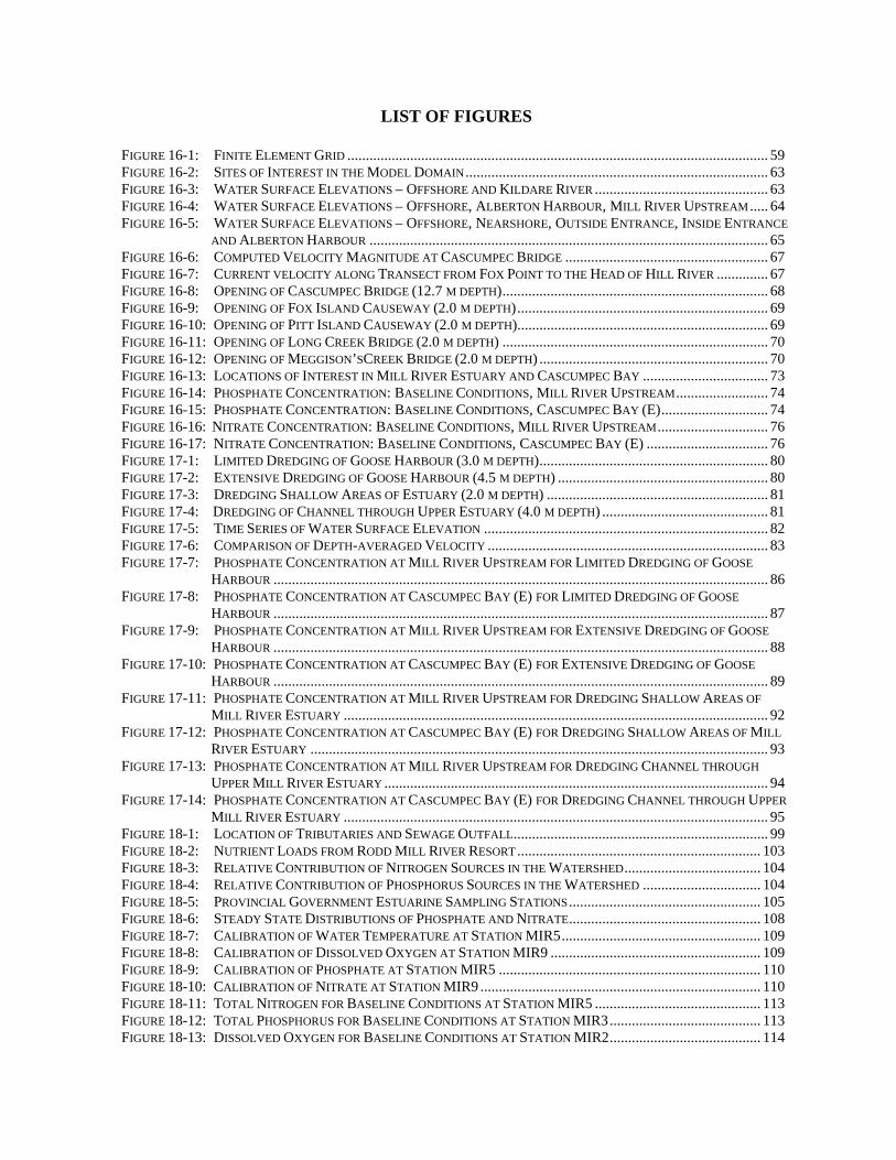
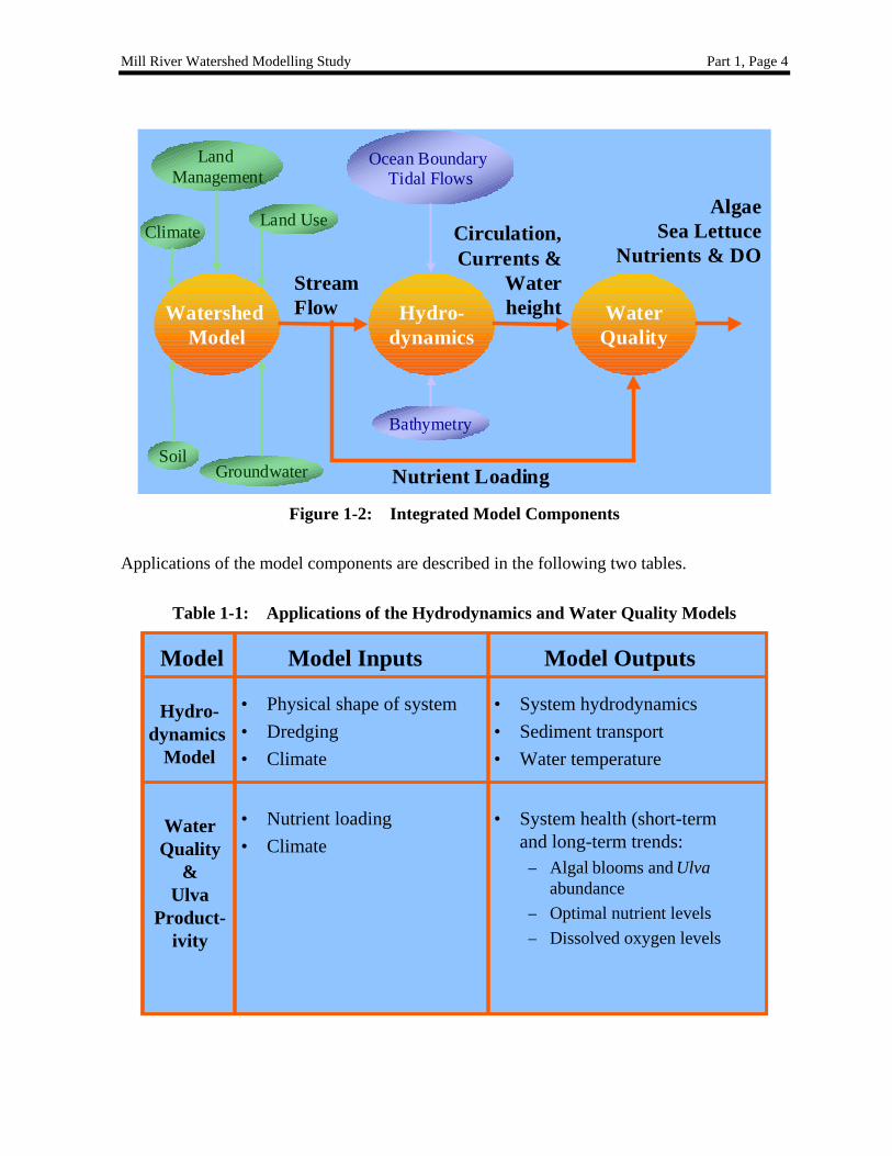
freshwater enters the estuary. Identifying Optimum Strategy (Activity #4) The scope of the project includes modelling various combinations of beneficial modifications for each of the above three activities to identify their combined benefit and ultimately, the most beneficial modification strategy. Since long-term sediment and nutrient loading of the estuary is of primary interest, modelling of a worst case scenario based on a single extreme event, such as a severe rainstorm, is outside the scope of work. Selection of the most ‘cost-effective’ solution is outside the scope of this study, since it would require a detailed cost-benefit analysis of the economics for each alternative. Since this is primarily a numerical modelling study, the ‘optimized solution’ is the most beneficial strategy in terms of changes to the physical system and its effects on the nutrient loading, sedimentation losses and biological processes. 1.4 MODELLING APPROACH The Mill River model is conceptualized as an integrated hydrodynamics, water quality, and watershed model. Generic models are adapted to the specific ecosystem, though calibration of model output to measured data, ideally for a data set spanning several years. The overall model is intended to be a robust predictive tool, aiding decision-makers in integrated management of the sensitive ecosystems and their resources. The integrated model is illustrated in the following figure. The watershed model provides stream flows to the hydrodynamics model, and nutrient and pesticide loads to the water quality model, based on climate, soil type, groundwater transport characterization, land use, and land management. The hydrodynamics model is used to represent coastal ecosystem circulation, tidal elevations, and currents. Based on this representation of water transport in the estuary, transport and reaction kinetics of chemical and biological constituents are modeled by the coupled water quality model.


Watershed Model

Hydro-dynamics

WaterQuality

ClimateLand Use

Land Management

SoilGroundwater

Stream Flow

Ocean Boundary Tidal Flows

Bathymetry

Nutrient Loading

Circulation,Currents &

Waterheight

AlgaeSea Lettuce

Nutrients & DO

Figure 1-2: Integrated Model Components

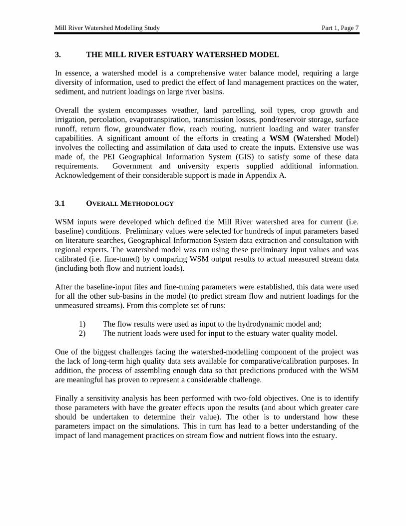
Applications of the model components are described in the following two tables.

Table 1-1: Applications of the Hydrodynamics and Water Quality Models

Model Model Inputs Model Outputs

Hydro-dynamics

Model

• Physical shape of system• Dredging• Climate

• System hydrodynamics• Sediment transport• Water temperature

WaterQuality

&Ulva

Product-ivity

• Nutrient loading• Climate

• System health (short-termand long-term trends:– Algal blooms and Ulva

abundance– Optimal nutrient levels– Dissolved oxygen levels


Table 1-2: Applications of the Watershed Model

Model Model Inputs Model Outputs

Water-shedModel

• Climate• Management Practices

– Crop rotation– Buffer zones– Fertilizers & Irrigation– Erosion prevention– Livestock

• Stream Flows• Nutrient loading levels• Run-off & Erosion

1.5 ORGANIZATION OF THE REPORT For the current study, the watershed model provided input data on stream flows and nutrient loads to the hydrodynamic and water quality models. It was also used to investigate the effect of reducing input sediment and nutrient loads from various sources in the Mill River Watershed. Modelling of the hydrodynamics and water quality of Mill River Estuary is presented in Part 2 of this report. The numerical modelling and results for Activities #1 through #4 are described in Sections 15 through 18, respectively. Conclusions are presented in Part 2, Section 19 and recommendations for the most beneficial modification strategy are summarized in the same section.


2. INTRODUCTION TO WATERSHED MODELLING The interdisciplinary nature and increasing complexities of environmental and water-resource problems encourage the use of numerical modelling tools incorporating extensive knowledge bases from a broad range of scientific disciplines. These disciplines include nutrient load modelling, crop selection/rotation impact, land management/usage assessments, and, ultimately, the combined effects and interrelationships that affect sediment and water transport and, indirectly, nutrient loading into a river system. Pesticide modelling, another capability of watershed modelling, was not performed as part of the Mill River analysis. Watershed-modelling efforts were used to initially predict inflow rates and establish initial nutrient concentrations for the fresh water bodies flowing into the Mill River estuary. A ranking of fresh water inflows was performed to establish the most significant streams. The inflow rates were used as inputs into the hydrodynamic model with the nutrient loads used as input into the water quality model. The watershed software system used to model the Mill River watershed area was SWAT (Soil and Water Assessment Tool) 2000 (J.G. Arnold et al, 1998). This section of the report discusses the watershed modelling in detail and presents the results.


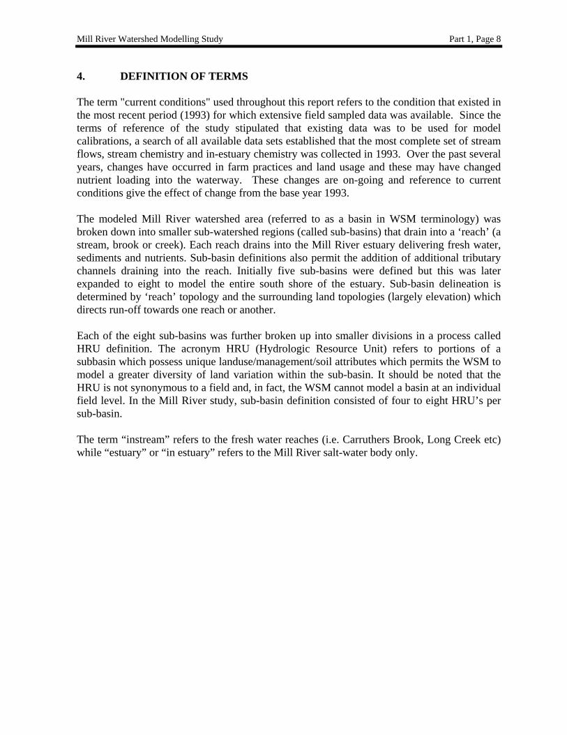
3. THE MILL RIVER ESTUARY WATERSHED MODEL In essence, a watershed model is a comprehensive water balance model, requiring a large diversity of information, used to predict the effect of land management practices on the water, sediment, and nutrient loadings on large river basins. Overall the system encompasses weather, land parcelling, soil types, crop growth and irrigation, percolation, evapotranspiration, transmission losses, pond/reservoir storage, surface runoff, return flow, groundwater flow, reach routing, nutrient loading and water transfer capabilities. A significant amount of the efforts in creating a WSM (Watershed Model) involves the collecting and assimilation of data used to create the inputs. Extensive use was made of, the PEI Geographical Information System (GIS) to satisfy some of these data requirements. Government and university experts supplied additional information. Acknowledgement of their considerable support is made in Appendix A. 3.1 OVERALL METHODOLOGY WSM inputs were developed which defined the Mill River watershed area for current (i.e. baseline) conditions. Preliminary values were selected for hundreds of input parameters based on literature searches, Geographical Information System data extraction and consultation with regional experts. The watershed model was run using these preliminary input values and was calibrated (i.e. fine-tuned) by comparing WSM output results to actual measured stream data (including both flow and nutrient loads). After the baseline-input files and fine-tuning parameters were established, this data were used for all the other sub-basins in the model (to predict stream flow and nutrient loadings for the unmeasured streams). From this complete set of runs:

1) The flow results were used as input to the hydrodynamic model and; 2) The nutrient loads were used for input to the estuary water quality model.

One of the biggest challenges facing the watershed-modelling component of the project was the lack of long-term high quality data sets available for comparative/calibration purposes. In addition, the process of assembling enough data so that predictions produced with the WSM are meaningful has proven to represent a considerable challenge. Finally a sensitivity analysis has been performed with two-fold objectives. One is to identify those parameters with have the greater effects upon the results (and about which greater care should be undertaken to determine their value). The other is to understand how these parameters impact on the simulations. This in turn has lead to a better understanding of the impact of land management practices on stream flow and nutrient flows into the estuary.


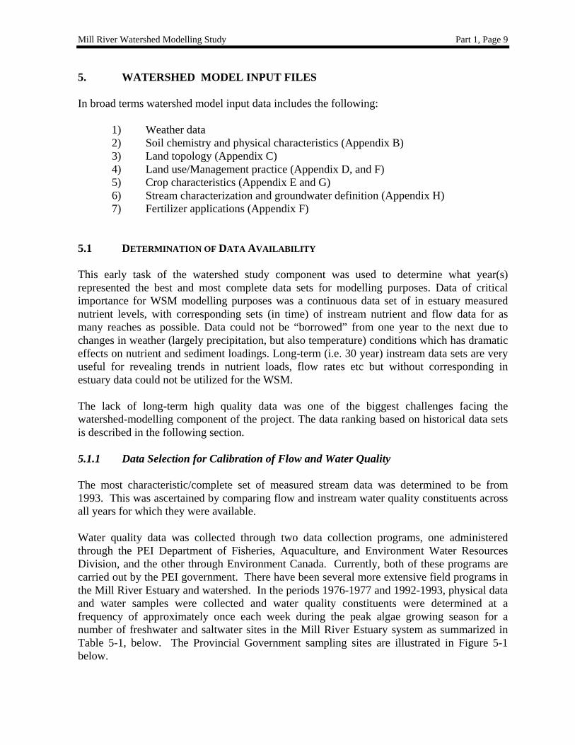
4. DEFINITION OF TERMS The term "current conditions" used throughout this report refers to the condition that existed in the most recent period (1993) for which extensive field sampled data was available. Since the terms of reference of the study stipulated that existing data was to be used for model calibrations, a search of all available data sets established that the most complete set of stream flows, stream chemistry and in-estuary chemistry was collected in 1993. Over the past several years, changes have occurred in farm practices and land usage and these may have changed nutrient loading into the waterway. These changes are on-going and reference to current conditions give the effect of change from the base year 1993. The modeled Mill River watershed area (referred to as a basin in WSM terminology) was broken down into smaller sub-watershed regions (called sub-basins) that drain into a ‘reach’ (a stream, brook or creek). Each reach drains into the Mill River estuary delivering fresh water, sediments and nutrients. Sub-basin definitions also permit the addition of additional tributary channels draining into the reach. Initially five sub-basins were defined but this was later expanded to eight to model the entire south shore of the estuary. Sub-basin delineation is determined by ‘reach’ topology and the surrounding land topologies (largely elevation) which directs run-off towards one reach or another.

Each of the eight sub-basins was further broken up into smaller divisions in a process called HRU definition. The acronym HRU (Hydrologic Resource Unit) refers to portions of a subbasin which possess unique landuse/management/soil attributes which permits the WSM to model a greater diversity of land variation within the sub-basin. It should be noted that the HRU is not synonymous to a field and, in fact, the WSM cannot model a basin at an individual field level. In the Mill River study, sub-basin definition consisted of four to eight HRU’s per sub-basin. The term “instream” refers to the fresh water reaches (i.e. Carruthers Brook, Long Creek etc) while “estuary” or “in estuary” refers to the Mill River salt-water body only.


5. WATERSHED MODEL INPUT FILES

In broad terms watershed model input data includes the following:

1) Weather data 2) Soil chemistry and physical characteristics (Appendix B) 3) Land topology (Appendix C) 4) Land use/Management practice (Appendix D, and F) 5) Crop characteristics (Appendix E and G) 6) Stream characterization and groundwater definition (Appendix H) 7) Fertilizer applications (Appendix F)

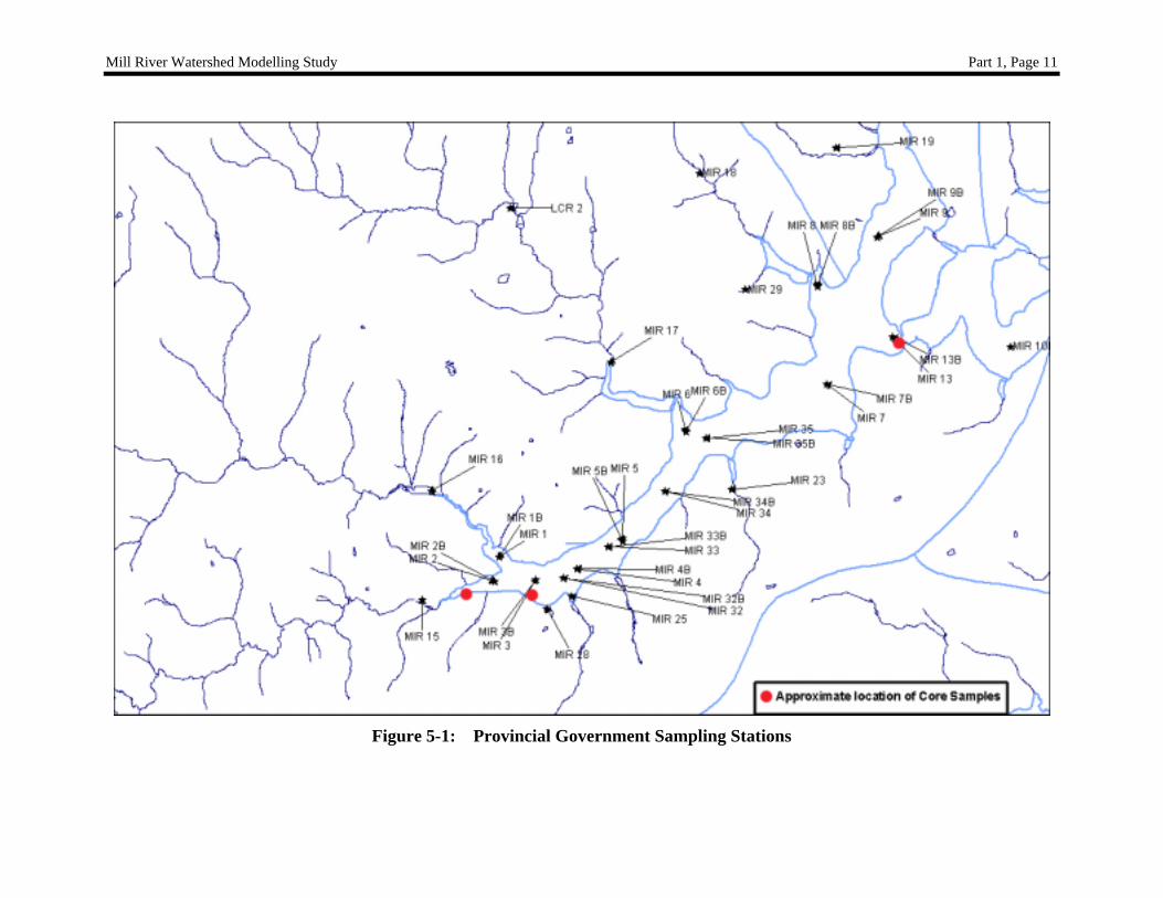
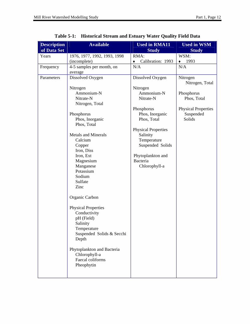
5.1 DETERMINATION OF DATA AVAILABILITY This early task of the watershed study component was used to determine what year(s) represented the best and most complete data sets for modelling purposes. Data of critical importance for WSM modelling purposes was a continuous data set of in estuary measured nutrient levels, with corresponding sets (in time) of instream nutrient and flow data for as many reaches as possible. Data could not be “borrowed” from one year to the next due to changes in weather (largely precipitation, but also temperature) conditions which has dramatic effects on nutrient and sediment loadings. Long-term (i.e. 30 year) instream data sets are very useful for revealing trends in nutrient loads, flow rates etc but without corresponding in estuary data could not be utilized for the WSM. The lack of long-term high quality data was one of the biggest challenges facing the watershed-modelling component of the project. The data ranking based on historical data sets is described in the following section. 5.1.1 Data Selection for Calibration of Flow and Water Quality The most characteristic/complete set of measured stream data was determined to be from 1993. This was ascertained by comparing flow and instream water quality constituents across all years for which they were available. Water quality data was collected through two data collection programs, one administered through the PEI Department of Fisheries, Aquaculture, and Environment Water Resources Division, and the other through Environment Canada. Currently, both of these programs are carried out by the PEI government. There have been several more extensive field programs in the Mill River Estuary and watershed. In the periods 1976-1977 and 1992-1993, physical data and water samples were collected and water quality constituents were determined at a frequency of approximately once each week during the peak algae growing season for a number of freshwater and saltwater sites in the Mill River Estuary system as summarized in Table 5-1, below. The Provincial Government sampling sites are illustrated in Figure 5-1 below.


The Mill River estuary is supplied with fresh water from many streams and brooks, the bulk coming via Carruthers and Cain’s Brooks, Long and Meggison’s Creeks and the Hill River. Of these, the only metered stream was Carruthers Brook. Included in these field measurements were daily stream flow data for Carruthers Brook and total nitrogen (TN) and total phosphorous (TP) for Carruthers Brook, Cain’s Brook and Long Creek. In addition instream estuary measurements for the calibration of the RMA11 estuarine water quality model were also known for 1993.


Figure 5-1: Provincial Government Sampling Stations


Table 5-1: Historical Stream and Estuary Water Quality Field Data

Description of Data Set

Available Used in RMA11 Study

Used in WSM Study

Years 1976, 1977, 1992, 1993, 1998 (incomplete)

RMA: ♦ Calibration: 1993

WSM: ♦ 1993

Frequency 4-5 samples per month, on average

N/A N/A

Parameters Dissolved Oxygen Nitrogen

Ammonium-N Nitrate-N Nitrogen, Total

Phosphorus Phos, Inorganic Phos, Total

Metals and Minerals

Calcium Copper Iron, Diss Iron, Ext Magnesium Manganese Potassium Sodium Sulfate Zinc

Organic Carbon Physical Properties

Conductivity pH (Field) Salinity Temperature Suspended Solids & Secchi Depth

Phytoplankton and Bacteria

Chlorophyll-a Faecal coliforms Pheophytin

Dissolved Oxygen

Nitrogen Ammonium-N Nitrate-N

Phosphorus Phos, Inorganic Phos, Total

Physical Properties

Salinity Temperature Suspended Solids

Phytoplankton and Bacteria

Chlorophyll-a

Nitrogen Nitrogen, Total

Phosphorus Phos, Total

Physical Properties Suspended Solids


5.1.2 Weather Data Although the WSM includes comprehensive weather generator capabilities, measured weather data is preferred. Specific 1993 weather data was purchased from the Atmospheric Environmental Service of Canada (AES). Where possible, O’Leary weather station data was used due to its proximity to the Mill River study area with Charlottetown weather station data used to supplement this data as necessary. Weather Data Station Daily Precipitation O’Leary Daily Temperature (Maximum and Minimum) O’Leary Daily Wind Speed Charlottetown Daily Humidity Charlottetown Daily Solar Radiation Charlottetown A data set spanning several decades, in addition to being prohibitively expensive to purchase, is of limited value, given only one good year (1993) of calibration data availability. 5.1.3 General Data Availability for WSM Input Files The WSM requires a wide range of inputs integrated across an extensive relational file system. The data requirements are described in more detail in Sections 5.3 – 5.8. Some of the input parameters are not readily available in published literature, or did not apply specifically to Prince Edward Island or the Mill River study area. Much of the data was collected through personal communications with PEI and Government of Canada civil servants/researchers and proved to be very time intensive. Details of these contributions are summarized in Appendix A. 5.2 USE OF THE PEI GEOGRAPHICAL INFORMATION SYSTEM 5.2.1 Land Use Data Availability As discussed further in Section 5.4, land use definition was available in the form of a MapInfo GIS database provided by the by PEI Department of Agriculture and Forestry Graphical Information System Division. A contract was signed to the effect that Martec would receive information limited to the Mill River estuary study area, and apply the information to the Mill River Watershed Modelling Study only. Forestry and agriculture were the two types of non-urban land use considered. Forestry data was available for 1935, 1958, 1990 based on aerial photography, and 1997-2000 satellite imagery. Agricultural land use data were available only for the period 1997-2000. The most complete data set most closely associated with the 1993 estuarine and stream field programs, was the 1997 satellite imagery. This data set was used to define Mill River watershed coverage by land use type.


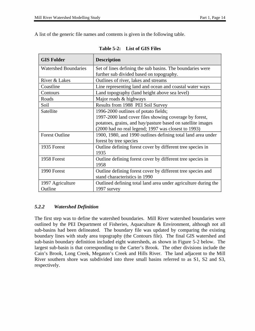
A list of the generic file names and contents is given in the following table.

Table 5-2: List of GIS Files

GIS Folder Description

Watershed Boundaries Set of lines defining the sub basins. The boundaries were further sub divided based on topography.

River & Lakes Outlines of river, lakes and streams Coastline Line representing land and ocean and coastal water ways Contours Land topography (land height above sea level) Roads Major roads & highways Soil Results from 1988 PEI Soil Survey Satellite 1996-2000 outlines of potato fields;

1997-2000 land cover files showing coverage by forest, potatoes, grains, and hay/pasture based on satellite images (2000 had no real legend; 1997 was closest to 1993)

Forest Outline 1900, 1980, and 1990 outlines defining total land area under forest by tree species

1935 Forest Outline defining forest cover by different tree species in 1935

1958 Forest Outline defining forest cover by different tree species in 1958

1990 Forest Outline defining forest cover by different tree species and stand characteristics in 1990

1997 Agriculture Outline

Outlined defining total land area under agriculture during the 1997 survey

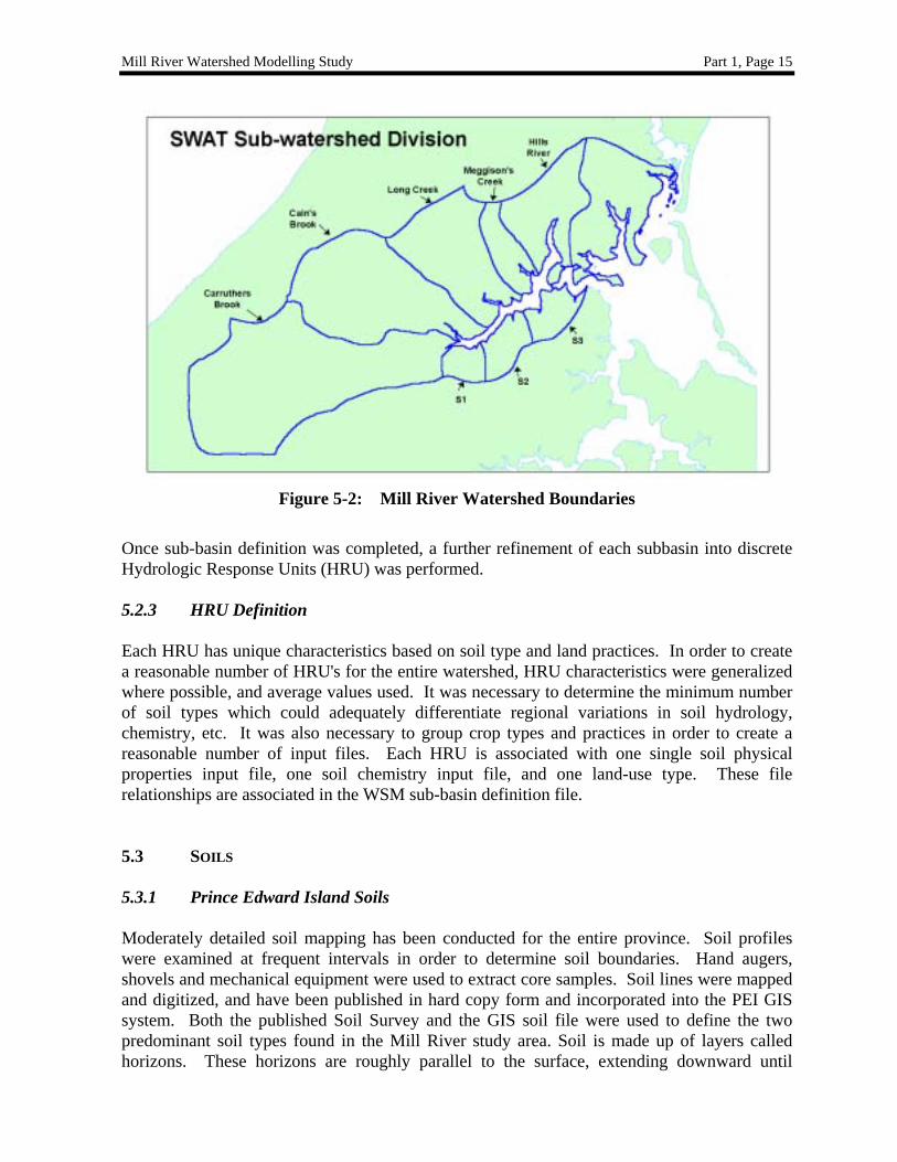
5.2.2 Watershed Definition The first step was to define the watershed boundaries. Mill River watershed boundaries were outlined by the PEI Department of Fisheries, Aquaculture & Environment, although not all sub-basins had been delineated. The boundary file was updated by comparing the existing boundary lines with study area topography (the Contours file). The final GIS watershed and sub-basin boundary definition included eight watersheds, as shown in Figure 5-2 below. The largest sub-basin is that corresponding to the Carter’s Brook. The other divisions include the Cain’s Brook, Long Creek, Megaton’s Creek and Hills River. The land adjacent to the Mill River southern shore was subdivided into three small basins referred to as S1, S2 and S3, respectively.


Figure 5-2: Mill River Watershed Boundaries

Once sub-basin definition was completed, a further refinement of each subbasin into discrete Hydrologic Response Units (HRU) was performed. 5.2.3 HRU Definition Each HRU has unique characteristics based on soil type and land practices. In order to create a reasonable number of HRU's for the entire watershed, HRU characteristics were generalized where possible, and average values used. It was necessary to determine the minimum number of soil types which could adequately differentiate regional variations in soil hydrology, chemistry, etc. It was also necessary to group crop types and practices in order to create a reasonable number of input files. Each HRU is associated with one single soil physical properties input file, one soil chemistry input file, and one land-use type. These file relationships are associated in the WSM sub-basin definition file. 5.3 SOILS 5.3.1 Prince Edward Island Soils Moderately detailed soil mapping has been conducted for the entire province. Soil profiles were examined at frequent intervals in order to determine soil boundaries. Hand augers, shovels and mechanical equipment were used to extract core samples. Soil lines were mapped and digitized, and have been published in hard copy form and incorporated into the PEI GIS system. Both the published Soil Survey and the GIS soil file were used to define the two predominant soil types found in the Mill River study area. Soil is made up of layers called horizons. These horizons are roughly parallel to the surface, extending downward until


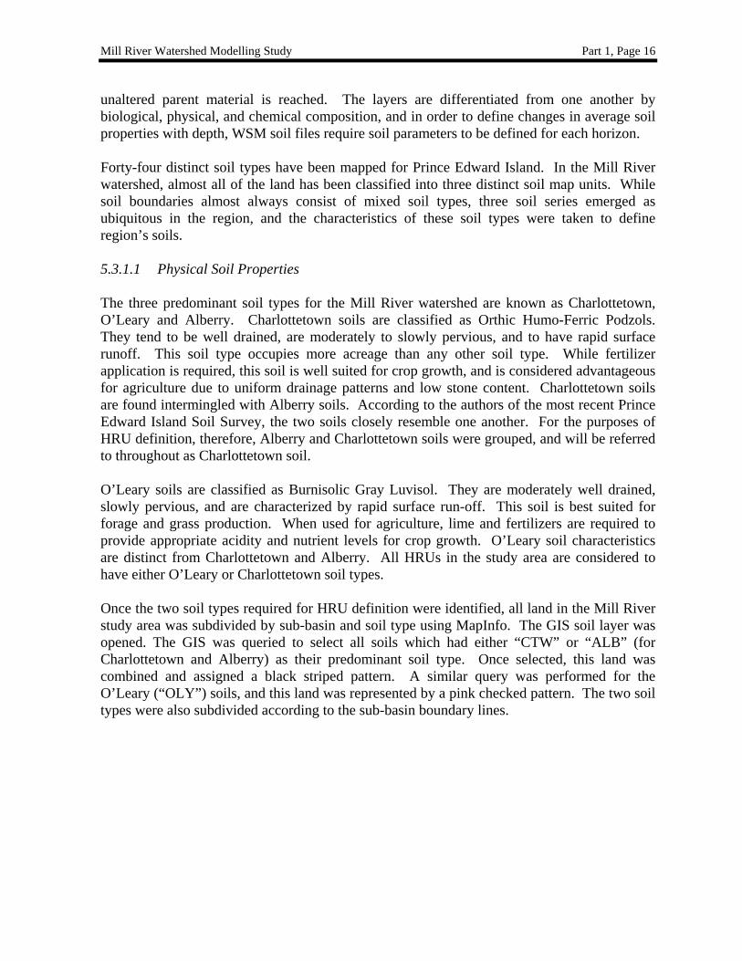
unaltered parent material is reached. The layers are differentiated from one another by biological, physical, and chemical composition, and in order to define changes in average soil properties with depth, WSM soil files require soil parameters to be defined for each horizon. Forty-four distinct soil types have been mapped for Prince Edward Island. In the Mill River watershed, almost all of the land has been classified into three distinct soil map units. While soil boundaries almost always consist of mixed soil types, three soil series emerged as ubiquitous in the region, and the characteristics of these soil types were taken to define region’s soils. 5.3.1.1 Physical Soil Properties The three predominant soil types for the Mill River watershed are known as Charlottetown, O’Leary and Alberry. Charlottetown soils are classified as Orthic Humo-Ferric Podzols. They tend to be well drained, are moderately to slowly pervious, and to have rapid surface runoff. This soil type occupies more acreage than any other soil type. While fertilizer application is required, this soil is well suited for crop growth, and is considered advantageous for agriculture due to uniform drainage patterns and low stone content. Charlottetown soils are found intermingled with Alberry soils. According to the authors of the most recent Prince Edward Island Soil Survey, the two soils closely resemble one another. For the purposes of HRU definition, therefore, Alberry and Charlottetown soils were grouped, and will be referred to throughout as Charlottetown soil. O’Leary soils are classified as Burnisolic Gray Luvisol. They are moderately well drained, slowly pervious, and are characterized by rapid surface run-off. This soil is best suited for forage and grass production. When used for agriculture, lime and fertilizers are required to provide appropriate acidity and nutrient levels for crop growth. O’Leary soil characteristics are distinct from Charlottetown and Alberry. All HRUs in the study area are considered to have either O’Leary or Charlottetown soil types. Once the two soil types required for HRU definition were identified, all land in the Mill River study area was subdivided by sub-basin and soil type using MapInfo. The GIS soil layer was opened. The GIS was queried to select all soils which had either “CTW” or “ALB” (for Charlottetown and Alberry) as their predominant soil type. Once selected, this land was combined and assigned a black striped pattern. A similar query was performed for the O’Leary (“OLY”) soils, and this land was represented by a pink checked pattern. The two soil types were also subdivided according to the sub-basin boundary lines.


Figure 5-3: Mill River Watershed Soil Divisions for WSM

Transport of water and air, and water cycling through the soil horizons is governed by soil physical properties. Each HRU has an associated soil file (either O’Leary or Charlottetown). The physical properties values for the soil profiles are further detailed in Appendix B. 5.3.1.2 Soil Chemistry for WSM Input File Definition Soil properties can be divided into two categories, physical and chemical characteristics, with the chemical characteristics establish the initial chemical levels in the soil. Two distinct chemistry profiles were used depending on land cover (forested or agricultural use). Each soil horizon was given an initial concentration for inorganic N (mg/kg), organic N (mg/kg), soluble P (mg/kg) and organic P (mg/kg). The chemistry information was obtained by contacting several expert sources at Agriculture and Agri-Food Canada, PEI DAF, University of New Brunswick, and the Eastern Canada Soil and Water Conservation Centre. 5.4 LAND USE BY AREA FOR WSM HRU INPUT FILE DEFINITION HRU divisions are also associated with land use. In the case of the Mill River area, land use was either agriculture or forestry. Agricultural land use was grouped into three crop types: potato, hay pastures, and grains. It was necessary to generalize the crop type in order to maintain a workable number of HRUs.


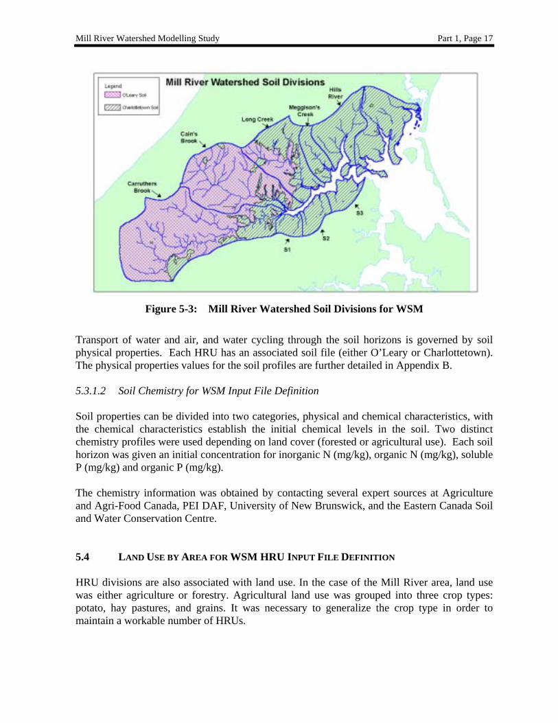
The process for defining land use by crop type is similar to that used for defining soil area by watershed sub-basin. MapInfo was used to select land by land use. There were eight possible types of land use defined for each sub-basin (see Table 5-3, below). The MapInfo query feature was used to select, group, and assign colours according to land use for each soil type. For example, queries were performed to select all potato crops on Charlottetown soil for Carruther’s Brook sub-basin. For each sub-basin, queries were repeated for the three other land use types (Grains, Hay & Pasture, and Forest), by soil coverage. HRU parameters for the watershed model are specified in Appendix C.

Table 5-3: Land Use for each Sub-basin Corresponding to Soil Type

Forest Potato Grains Hay & Pasture Other

Charlottetown 1.80 2.55 1.40 0.71 2.88O'Leary 29.35 4.24 3.14 4.71 2.45



Charlottetown 0.59 2.42 1.05 1.25 0.56O'Leary

Charlottetown 2.15 4.30 4.20 2.39 0.92O'Leary 0.01




Total Modelled Watershed Area 136.28

4.73

4.48

Total Sub-basin Area (km 2 )

30.86

19.99

5.858

13.96

S2

S3

Sub-basin

Cain's Brook

Long Creek

Meggissons Creek

Hills River

Carruther's Brook

Land Use (km 2 )

53.24

Soil Type

S1 3.17

‘Other’ refers to land use of non-major crop types, live stock farms, roads and residential areas. 5.5 SUBBASIN AND HYDROLOGICAL RESPONSE UNITS (HRU) The associated WSM input files for Hydrologic Response Units, namely the HRU file, the soil type file, the soil chemistry file, and the land management file are linked in the WSM sub-basin file, as illustrated in the table below. As illustrated in the file, each sub-basin can have a maximum of eight possible HRUs, based on four possible land uses over the two possible soil types. Forested land is always associated with the forest soil chemistry, all three types of agriculture are paired with the agricultural soil chemistry file.


Table 5-4: HRU Definitions

Soil Type Soil Chemistry Land Use Charlottetown Forest Mixed Forest Agriculture Potato Grains Hay and Pasture O’Leary Forest Mixed Forest Agriculture Potato Grains Hay and Pasture

5.6 REACH DEFINITION As shown in Figure 5-4, each sub-basin contains a reach varying in length from 10.6 km to 1.25 km. Each individual reach is defined by a slope, an average depth and width, total length, hydraulic conductivity and erosion characteristics.

Figure 5-4: Sub-basin Reaches for Watershed Model


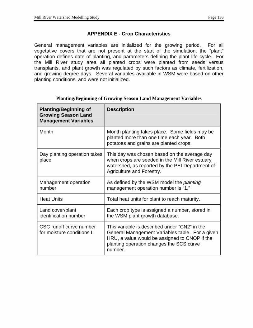
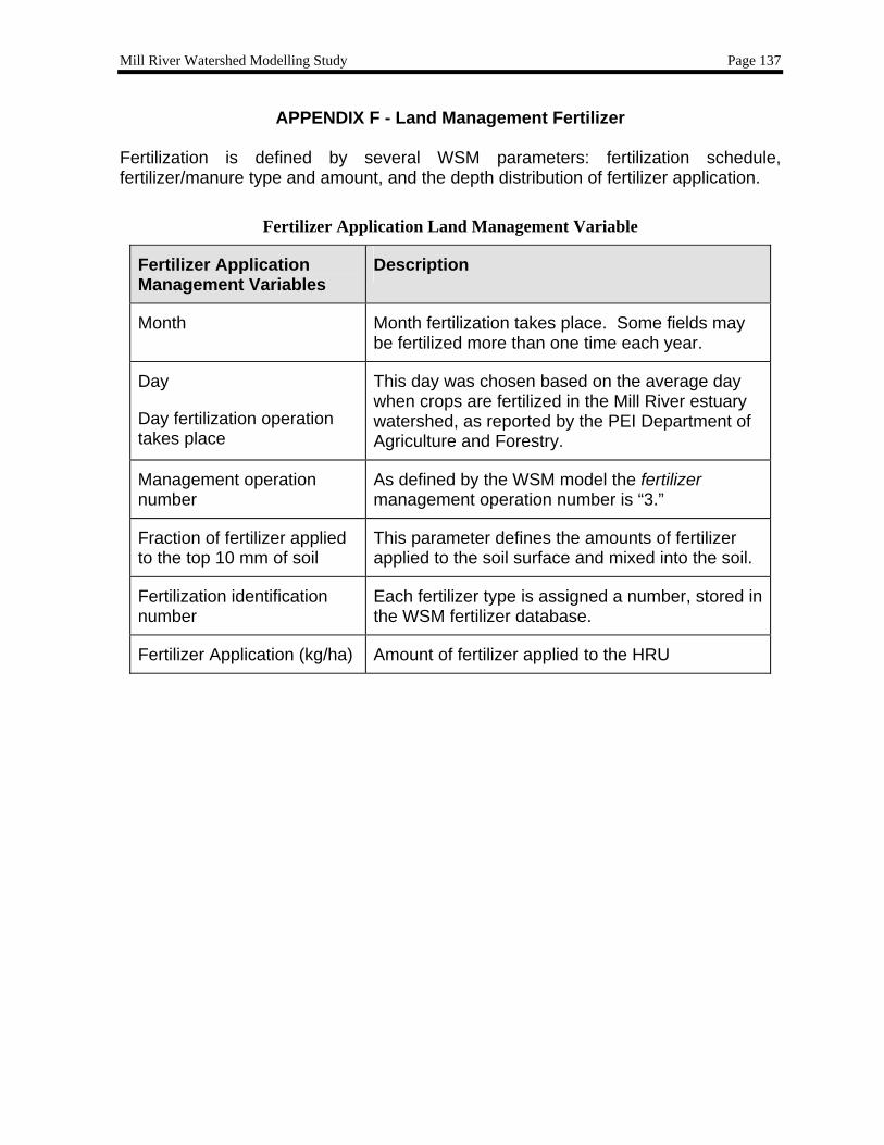
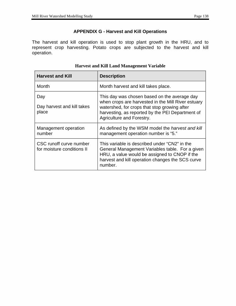
5.7 LAND MANAGEMENT DEFINITION FOR THE WSM HRU definition includes a parameter to represent the fraction of sub-basin area covered by each of the four vegetative covers and their associated soil types. A primary goal of environmental modelling is to assess the impact of anthropogenic activities on a given system. Central to this is the itemization of land and water management practices taking place in the water shed. Relevant to this study, the land management files contain input data to describe the planting, harvesting, nutrient applications, and tillage operations. Irrigation and pesticide applications were not modeled as part of the Mill River study. Land management practises specified for the Mill River WSM model included:

• Planting/beginning of growing season – detailed in Appendix E. • Fertilizer application – detailed in Appendix F. • Harvest and crop kill – detailed in Appendix G. • Harvest only – detailed in Appendix G. • Tillage – detailed in Appendix H.

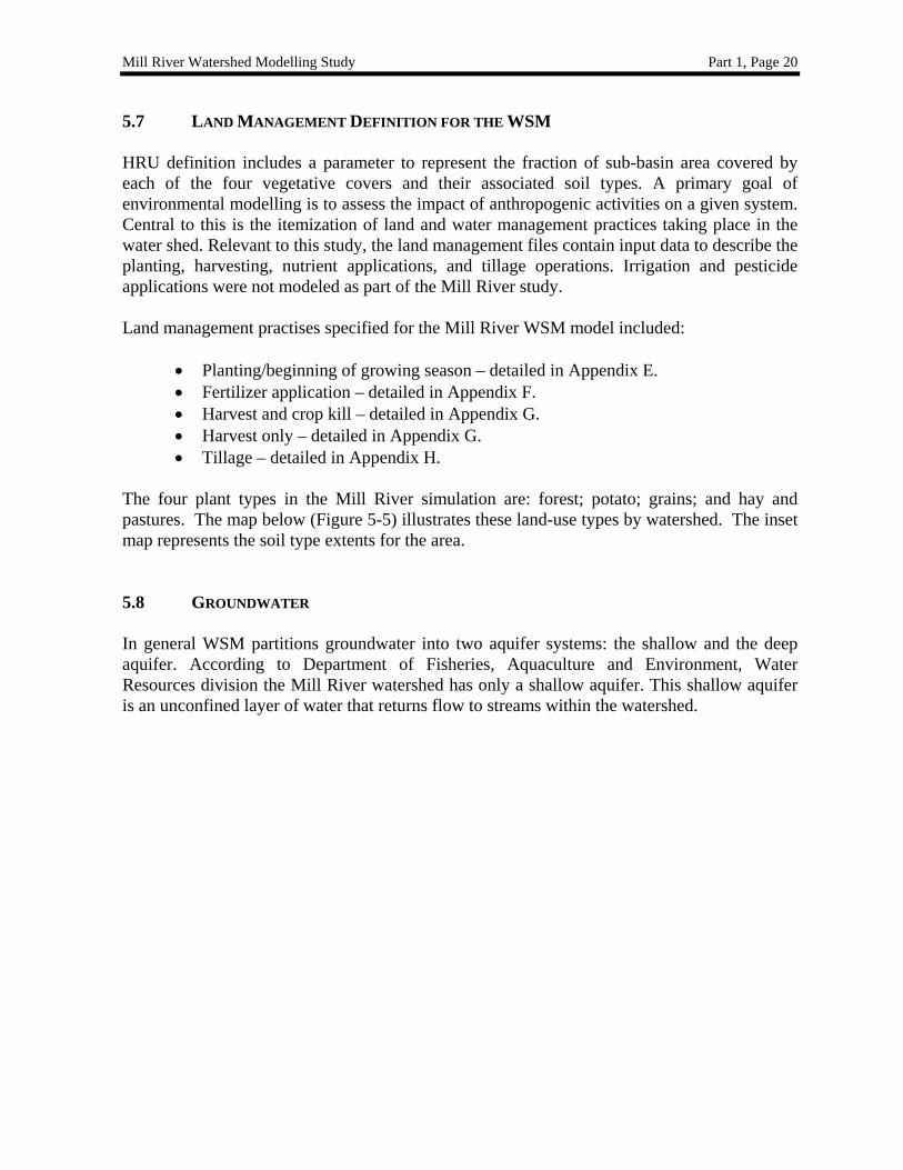
The four plant types in the Mill River simulation are: forest; potato; grains; and hay and pastures. The map below (Figure 5-5) illustrates these land-use types by watershed. The inset map represents the soil type extents for the area. 5.8 GROUNDWATER In general WSM partitions groundwater into two aquifer systems: the shallow and the deep aquifer. According to Department of Fisheries, Aquaculture and Environment, Water Resources division the Mill River watershed has only a shallow aquifer. This shallow aquifer is an unconfined layer of water that returns flow to streams within the watershed.


Figure 5-5: Sub-watershed Division Based on 1997 GIS Land Management


6. CALIBRATION OF WSM TO KNOWN CONDITIONS After all the initial input parameters were defined, preliminary WSM runs were performed. The calibration processes consisted of:

• Basic water balance followed by total water flow calibration • Nutrient calibration

Only one stream, Carruthers, had daily long-term stream flow measurements so this was used as the water balance calibration standard. Initial calibrations efforts indicated that using only one year of weather data was not optimal leading to some calibration errors early in the process. In effect, the simulation was cold started on January 1 and took several months to settle down. During this period the soil becomes wetted, the water table forms and a run-off conditions begin to occur. This was compounded by the fact that much of precipitation in January and February is in the form of snow, presenting additional problems when calibrating the spring run-off parameters. As a result WSM was predicting low flow rates. This situation was remedied by replicating the 1993 data as pseudo 1992 data and running a two-year simulation. Major tuning factors that had to be adjusted to achieve a good correlation between measured and predicted data are discussed in the following sections. 6.1 STREAM FLOW CALIBRATION

For stream flow calibration, the tuneable parameters that had to be adjusted to correctly model the flow were: • Lag time – the time between precipitation falling and eventual passage to the stream • Snow melt temperatures – adjusted to correctly model the spring run off • Water Table Depth - to establish correct baseflow values • Channel Hydraulic Conductivity Factor – to adjust the water losses through the reach Stream flow was calibrated first on a monthly basis, then refined to a daily basis. It is very important to correctly balance the total stream flow between surface runoff and baseflow rates to be able to correctly model the nutrient loadings. The surface runoff was initially calibrated by adjusting the curve number (based on land usage) and was further fine-tuned with a soil evaporation compensation factor and a soil available water capacity (performed at an HRU level). In addition, the baseflow rates (also known as sub-surface rates) were adjusted via a groundwater movement factor. Several cycles through the tuning process were required to generate the optimal solution. Once the temporal flows were correctly modelled the transmission losses values for channel conductivity (performed at a sub-basin level) were adjusted to correct a recession problem (the stream was draining too quickly). And finally the snow melt rates had to be fine tuned to better match the snow melt months.


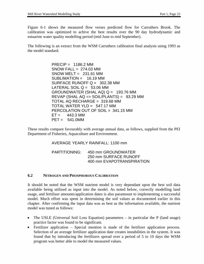
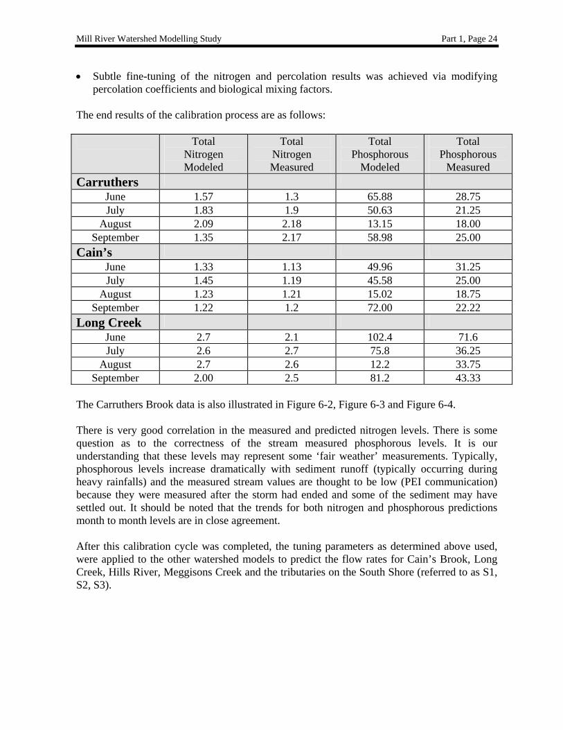
Figure 6-1 shows the measured flow verses predicted flow for Carruthers Brook. The calibration was optimized to achive the best results over the 90 day hydrodynamic and estuarine water quality modelling period (mid June to mid September). The following is an extract from the WSM Carruthers calibration final analysis using 1993 as the model standard.

PRECIP = 1186.2 MM SNOW FALL = 274.03 MM SNOW MELT = 231.61 MM SUBLIMATION = 16.19 MM SURFACE RUNOFF Q = 302.38 MM LATERAL SOIL Q = 53.06 MM GROUNDWATER (SHAL AQ) Q = 193.76 MM REVAP (SHAL AQ => SOIL/PLANTS) = 93.29 MM TOTAL AQ RECHARGE = 319.68 MM TOTAL WATER YLD = 547.17 MM PERCOLATION OUT OF SOIL = 341.15 MM ET = 443.3 MM PET = 541.0MM

These results compare favourably with average annual data, as follows, supplied from the PEI Department of Fisheries, Aquaculture and Environment.

AVERAGE YEARLY RAINFALL: 1100 mm PARTITIONING: 450 mm GROUNDWATER

250 mm SURFACE RUNOFF 400 mm EVAPOTRANSPIRATION

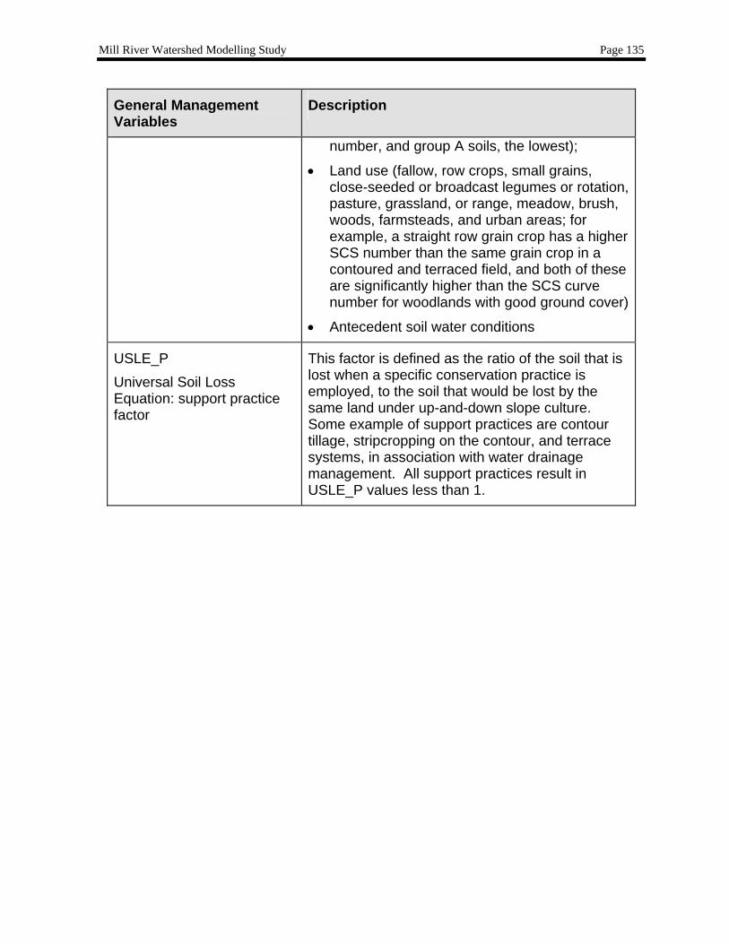
6.2 NITROGEN AND PHOSPHOROUS CALIBRATION It should be noted that the WSM nutrient model is very dependant upon the best soil data available being utilized as input into the model. As noted below, correctly modelling land usage, and fertilizer amounts/application dates is also paramount to implementing a successful model. Much effort was spent in determining the soil values as documented earlier in this chapter. After confirming the input data was as best as the information available, the nutrient model was tuned as follows: • The USLE (Universal Soil Loss Equation) parameters – in particular the P (land usage)

practice factor was found to be significant. • Fertilizer application – Special mention is made of the fertilizer application process.

Selection of an average fertilizer application date creates instabilities in the system. It was found that by introducing the fertilizers spread over a period of 5 to 10 days the WSM program was better able to model the measured values.


• Subtle fine-tuning of the nitrogen and percolation results was achieved via modifying percolation coefficients and biological mixing factors.

The end results of the calibration process are as follows: Total

Nitrogen Modeled

Total Nitrogen Measured

Total Phosphorous

Modeled

Total Phosphorous

Measured Carruthers

June 1.57 1.3 65.88 28.75 July 1.83 1.9 50.63 21.25

August 2.09 2.18 13.15 18.00 September 1.35 2.17 58.98 25.00

Cain’s June 1.33 1.13 49.96 31.25 July 1.45 1.19 45.58 25.00


Long Creek June 2.7 2.1 102.4 71.6 July 2.6 2.7 75.8 36.25


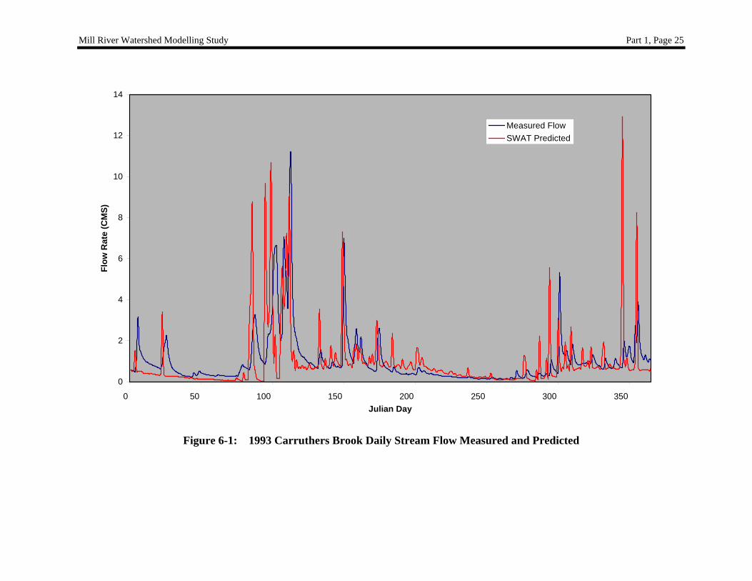
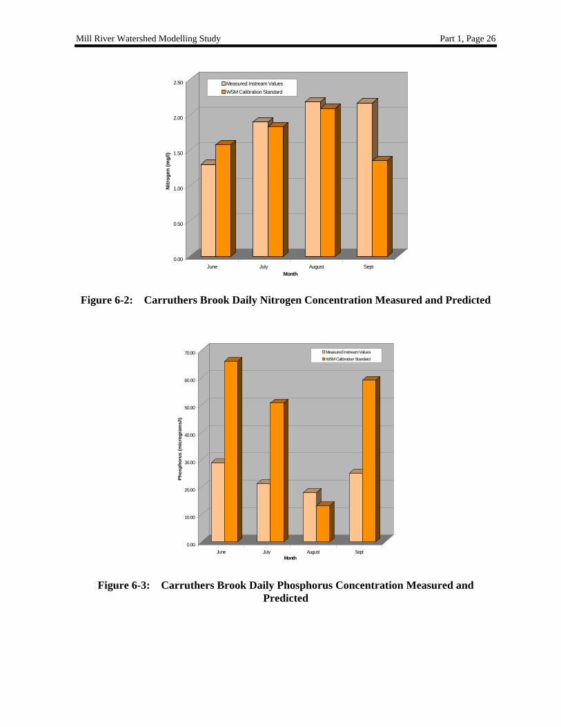
The Carruthers Brook data is also illustrated in Figure 6-2, Figure 6-3 and Figure 6-4. There is very good correlation in the measured and predicted nitrogen levels. There is some question as to the correctness of the stream measured phosphorous levels. It is our understanding that these levels may represent some ‘fair weather’ measurements. Typically, phosphorous levels increase dramatically with sediment runoff (typically occurring during heavy rainfalls) and the measured stream values are thought to be low (PEI communication) because they were measured after the storm had ended and some of the sediment may have settled out. It should be noted that the trends for both nitrogen and phosphorous predictions month to month levels are in close agreement. After this calibration cycle was completed, the tuning parameters as determined above used, were applied to the other watershed models to predict the flow rates for Cain’s Brook, Long Creek, Hills River, Meggisons Creek and the tributaries on the South Shore (referred to as S1, S2, S3).


0

2

4

6

8

10

12

14

0 50 100 150 200 250 300 350Julian Day

Flow

Rat

e (C

MS)

Measured FlowSWAT Predicted

Figure 6-1: 1993 Carruthers Brook Daily Stream Flow Measured and Predicted


0.00

0.50

1.00

1.50

2.00

2.50

Nitr

ogen

(mg/

l)

June July August SeptMonth

Measured Instream ValuesWSM Calibration Standard

Figure 6-2: Carruthers Brook Daily Nitrogen Concentration Measured and Predicted

0.00

10.00

20.00

30.00

40.00

50.00

60.00

70.00

Phos

phor

us (m

icro

gram

s/l)


Measured Instream ValuesWSM Calibration Standard

Figure 6-3: Carruthers Brook Daily Phosphorus Concentration Measured and

Predicted


0

10

20

30

40

50

60

70

Phos

phor

us (m

icro

gram

s/l)


Other P

Phosphate

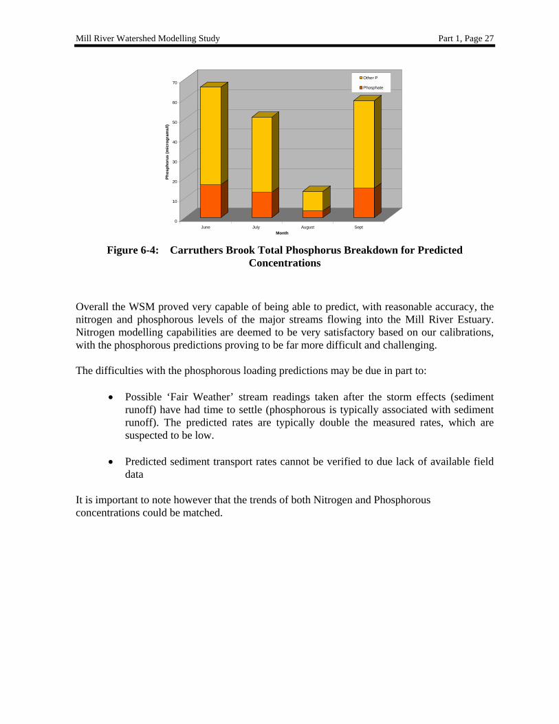
Figure 6-4: Carruthers Brook Total Phosphorus Breakdown for Predicted

Concentrations

Overall the WSM proved very capable of being able to predict, with reasonable accuracy, the nitrogen and phosphorous levels of the major streams flowing into the Mill River Estuary. Nitrogen modelling capabilities are deemed to be very satisfactory based on our calibrations, with the phosphorous predictions proving to be far more difficult and challenging. The difficulties with the phosphorous loading predictions may be due in part to:

• Possible ‘Fair Weather’ stream readings taken after the storm effects (sediment

runoff) have had time to settle (phosphorous is typically associated with sediment runoff). The predicted rates are typically double the measured rates, which are suspected to be low.

• Predicted sediment transport rates cannot be verified to due lack of available field

data It is important to note however that the trends of both Nitrogen and Phosphorous concentrations could be matched.


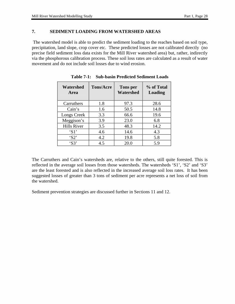
7. SEDIMENT LOADING FROM WATERSHED AREAS The watershed model is able to predict the sediment loading to the reaches based on soil type, precipitation, land slope, crop cover etc. These predicted losses are not calibrated directly (no precise field sediment loss data exists for the Mill River watershed area) but, rather, indirectly via the phosphorous calibration process. These soil loss rates are calculated as a result of water movement and do not include soil losses due to wind erosion.

Table 7-1: Sub-basin Predicted Sediment Loads

Watershed Area

Tons/Acre Tons per Watershed

% of Total Loading

Carruthers 1.8 97.3 28.6 Cain’s 1.6 50.5 14.8

Longs Creek 3.3 66.6 19.6 Meggison’s 3.9 23.0 6.8 Hills River 3.5 48.3 14.2

‘S1’ 4.6 14.6 4.3 ‘S2’ 4.2 19.8 5.8 ‘S3’ 4.5 20.0 5.9

The Carruthers and Cain’s watersheds are, relative to the others, still quite forested. This is reflected in the average soil losses from those watersheds. The watersheds ‘S1’, ‘S2’ and ‘S3’ are the least forested and is also reflected in the increased average soil loss rates. It has been suggested losses of greater than 3 tons of sediment per acre represents a net loss of soil from the watershed. Sediment prevention strategies are discussed further in Sections 11 and 12.


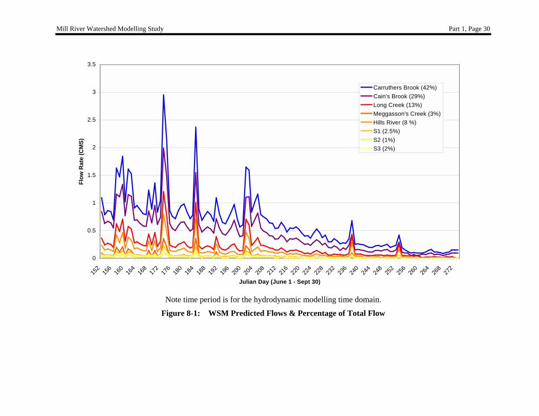
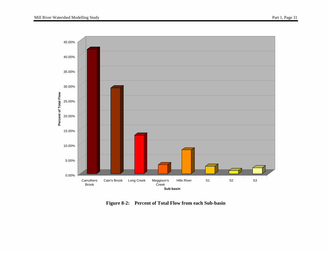
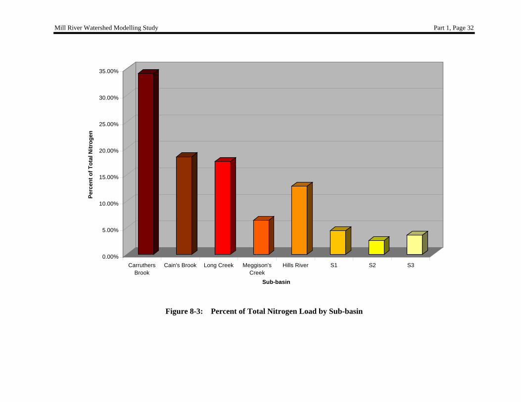
8. RESULTS Figure 8-1 and Figure 8-2 illustrate the relative flow rates of the eight major reaches (defining the eight sub-basins) that drain into the Mill River estuary. Carruthers Brook represents approximately 40% of the total drainage, with the combination of Carruthers Brook, Cain’s Brook and Long Creek accounting for 84%. The total mass loading for Nitrogen is shown in Figure 8-3. Carruthers Brook accounts for nearly 35% of the total nitrogen entering the estuary, with Cain’s Brook, and Long Creek accounting for approximately 19% and 18% respectively. Hill’s River while contributing 8% of the total flow, supplies 12% of the total nitrogen probably due to heavy agricultural use of the surrounding land. The total mass loading Phosphorous (Figure 8-4) follows a similar trend; Carruthers Brook represents 27%, Cains Brook 16%, Long Creek 15% and Hills River 14%. An add-on module to the WSM, a code known as QUAL2E, was invoked to further model the Nitrogen cycle (convert Total N into NH3, NO4, NH2) producing a smoother and more expedient transition into the RMA11 estuarine water quality model. Qual2e standard defaults were used for the simulation parameters with the objective, as above, of creating a better coupling procedure to the RMA11 code.


0

0.5

1

1.5

2

2.5

3

3.5

152

156

160

164

168

172

176

180

184

188

192

196

200

204

208

212

216

220

224

228

232

236

240

244

248

252

256

260

264

268

272

Julian Day (June 1 - Sept 30)

Flow

Rat

e (C

MS)

Carruthers Brook (42%)Cain's Brook (29%)Long Creek (13%)Meggasson's Creek (3%)Hills River (8 %)S1 (2.5%)S2 (1%)S3 (2%)

Note time period is for the hydrodynamic modelling time domain.

Figure 8-1: WSM Predicted Flows & Percentage of Total Flow


0.00%

5.00%

10.00%

15.00%

20.00%

25.00%

30.00%

35.00%

40.00%

45.00%

Perc

ent o

f Tot

al F

low

CarruthersBrook

Cain's Brook Long Creek Meggison'sCreek

Hills River S1 S2 S3

Sub-basin

Figure 8-2: Percent of Total Flow from each Sub-basin


0.00%

5.00%

10.00%

15.00%

20.00%

25.00%

30.00%

35.00%

Perc

ent o

f Tot

al N

itrog

en

CarruthersBrook



Sub-basin

Figure 8-3: Percent of Total Nitrogen Load by Sub-basin


0.00%

5.00%

10.00%

15.00%

20.00%

25.00%

30.00%

Perc

ent o

f Tot

al P

hosp

horu

s

CarruthersBrook



Sub-basin

Figure 8-4: Percent of Total Phosphorus Load by Sub-basin


8.1 SENSITIVITY ANALYSIS FOR WSM RESULTS Sensitivity Analysis is the study of how the variation in the output of a model (numerical or otherwise) can be apportioned, qualitatively or quantitatively, to different sources of variation. Sensitivity Analysis (SA) aims to ascertain how the model depends upon the information fed into it, upon its structure and upon the framing assumptions made to build it. This information can be invaluable, as

• Different uncertainties impact differently on the reliability, the robustness and the efficiency of the model.

• Different level of acceptance (by the decision-makers and stakeholders) may be

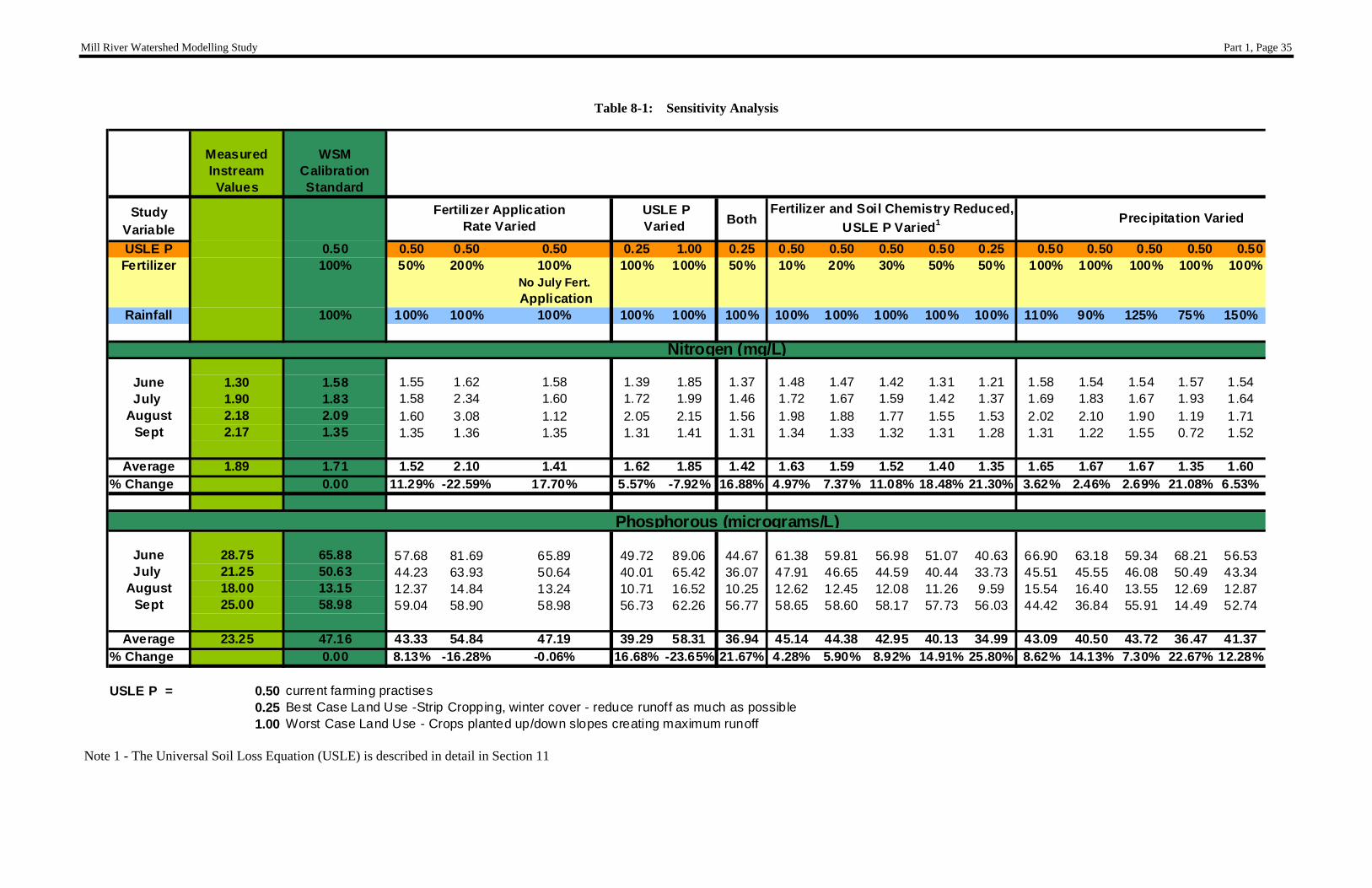
attached to different types of uncertainty. Originally, SA was created to deal simply with uncertainties in the input variables and model parameters. Over the course of time the ideas have been extended to incorporate model conceptual uncertainty, i.e. uncertainty in model structures, assumptions and specifications. As a whole, SA is used to increase the confidence in the model and its predictions, by providing an understanding of how the model response variables respond to changes in the inputs, be they data used to calibrate it, model structures, or factors, i.e. the model independent variables. A sensitivity analysis was performed on the Carruthers Brook data set. As mentioned earlier, Carruthers Brook was chosen as the calibration standard because the ‘best’ measured data sets were associated with this brook. The sensitivity analysis was performed by changing the following parameters:

• Varying the fertilizer amounts (by 50% and 200%) • Varying the USLE P factor (using .25, .5 and 1., where .25 and 1. are the maximum

upper and lower values of the equation based on empirical studies) • Varying the Precipitation amount (+/- 10%, +/- 25%, +50% and –40%)

The results are presented in Table 8-1. Examining the averages of the 4 monthly values for which measured data exists indicates that the model is not particularly sensitive to large changes in any of its major input parameters. The maximum percent change is about 25% but overall the average % change is under 10%.


Table 8-1: Sensitivity Analysis

Measured WSMInstream CalibrationValues Standard

Study Variable

Both

USLE P 0.50 0.50 0.50 0.50 0.25 1.00 0.25 0.50 0.50 0.50 0.50 0.25 0.50 0.50 0.50 0.50 0.50Fertilizer 100% 50% 200% 100% 100% 100% 50% 10% 20% 30% 50% 50% 100% 100% 100% 100% 100%

No July Fert. Application

Rainfall 100% 100% 100% 100% 100% 100% 100% 100% 100% 100% 100% 100% 110% 90% 125% 75% 150%

June 1.30 1.58 1.55 1.62 1.58 1.39 1.85 1.37 1.48 1.47 1.42 1.31 1.21 1.58 1.54 1.54 1.57 1.54July 1.90 1.83 1.58 2.34 1.60 1.72 1.99 1.46 1.72 1.67 1.59 1.42 1.37 1.69 1.83 1.67 1.93 1.64

August 2.18 2.09 1.60 3.08 1.12 2.05 2.15 1.56 1.98 1.88 1.77 1.55 1.53 2.02 2.10 1.90 1.19 1.71Sept 2.17 1.35 1.35 1.36 1.35 1.31 1.41 1.31 1.34 1.33 1.32 1.31 1.28 1.31 1.22 1.55 0.72 1.52

Average 1.89 1.71 1.52 2.10 1.41 1.62 1.85 1.42 1.63 1.59 1.52 1.40 1.35 1.65 1.67 1.67 1.35 1.60% Change 0.00 11.29% -22.59% 17.70% 5.57% -7.92% 16.88% 4.97% 7.37% 11.08% 18.48% 21.30% 3.62% 2.46% 2.69% 21.08% 6.53%

June 28.75 65.88 57.68 81.69 65.89 49.72 89.06 44.67 61.38 59.81 56.98 51.07 40.63 66.90 63.18 59.34 68.21 56.53July 21.25 50.63 44.23 63.93 50.64 40.01 65.42 36.07 47.91 46.65 44.59 40.44 33.73 45.51 45.55 46.08 50.49 43.34

August 18.00 13.15 12.37 14.84 13.24 10.71 16.52 10.25 12.62 12.45 12.08 11.26 9.59 15.54 16.40 13.55 12.69 12.87Sept 25.00 58.98 59.04 58.90 58.98 56.73 62.26 56.77 58.65 58.60 58.17 57.73 56.03 44.42 36.84 55.91 14.49 52.74

Average 23.25 47.16 43.33 54.84 47.19 39.29 58.31 36.94 45.14 44.38 42.95 40.13 34.99 43.09 40.50 43.72 36.47 41.37

% Change 0.00 8.13% -16.28% -0.06% 16.68% -23.65% 21.67% 4.28% 5.90% 8.92% 14.91% 25.80% 8.62% 14.13% 7.30% 22.67% 12.28%

USLE P = 0.50 current farming practises0.25 Best Case Land Use -Strip Cropping, winter cover - reduce runoff as much as possible1.00 Worst Case Land Use - Crops planted up/down slopes creating maximum runoff

Nitrogen (mg/L)

Phosphorous (micrograms/L)

Precipitation VariedFertilizer and Soil Chemistry Reduced,

USLE P Varied1Fertilizer Application

Rate Varied USLE P Varied

Note 1 - The Universal Soil Loss Equation (USLE) is described in detail in Section 11


9. DISCUSSION OF MILL RIVER WATERSHED MODEL RESULTS Overall the WSM proved quite capable of being able to predict, with reasonable accuracy, the flow rates and nitrogen and phosphorous levels of the major streams flowing into the Mill River estuary. Nitrogen modelling capabilities are deemed to be very satisfactory based on the calibrations, while calibrating the phosphorous predictions proving to be far more difficult and challenging.

The difficulties with the phosphorous loadings may be due to: • ‘Fair Weather’ stream readings when measurements are taken after the storm

effects may have time to settle down (phosphorous is typically associated with sediment runoff). The predicted rates are typically double the measured rates, which we suspect are low.

• Predicted sediment transport rates cannot be verified to due lack of available field

data. It is important to note however that the trends of both nitrogen and phosphorous concentrations were matched throughout the study time period. The sensitivity analysis showed the effects of changing farming practices on the nitrogen and phosphorous entering the estuary system. Using the extreme case of a 50 % reduction of fertilizer application with the theoretically best land farming practices (i.e. strip cropping, terracing etc) saw a 21% reduction of nitrogen entering the Mill River system and a phosphorous reduction of 26% (based on comparisons to the 1993 study conditions). For review purposes the WSM predicted vs. measured (in brackets) for Carruthers Brook are as follows (see also Figure 6-2 and Figure 6-3):

Month N Predicted P Predicted N Measured P Measured

June 1.58 65.88 (1.3) (28.75) July 1.83 50.63 (1.9) (21.25)

August 2.09 13.15 (2.18) (18.00) September 1.35 59.00 (2.17) (25.00)

Several special case analysis were performed for the Carruthers Brook standard runs Special Case Scenario 1 assumes that all the land is forested, and thus, no fertilizer regime is applied to the model (Historical Soil Chemistry used)


Month N Predicted P Predicted

June 1.03 11.44 July 1.02 8.46

August 1.00 0.16 September 1.00 0.53

Note: the predicted nitrogen and phosphorous loadings decrease dramatically.

Special Case # 2 – 2/3 all fields are planted with potatoes, 1/6 grain and 1/6 hay – standard fertilizer regime is followed for that crop (Historical Soil Chemistry used)

Month N Predicted P Predicted

June 2.04 120.4084 July 2.20 86.73685

September 4.20 18.92798 August 1.50 80.11273

Note: the significant increases in both nitrogen and phosphorous levels


10. THE POTENTIAL OF WATERSHED MODELLING The WSM was used to carry out sensitivity studies on key WSM variables affecting nutrient loads. The rainfall was varied to see what impact it had on nutrient transport from fields to the estuary. Land management variables were also studied in order to identify which agricultural practices had the most potential to affect nutrient loading for practices accessible to agricultural planners. The amount of fertilizer applied, and the effect of using land management practices such as contouring were studied by systematically varying the relevant WSM parameters (see Section 8.1). The watershed model can be used to study the impact of many other climatic and land management practices as well. The long-term impact of climate change on nutrient cycling and primary productivity could be studied using the coupled watershed and water quality models. Region wide practices such as reforestation and wetlands acreage can be considered, as well as field-specific practices such as crop rotation, type and amount of fertilizer or manure applied, tillage and irrigation operations, winter plant residue coverage, and land management practices. In addition virtual settling ponds can be added to the freshwater steams to examine the potential effects on the nutrient and sediment loads. Urban sources of nutrients can also be included in the model, and scenarios can be optimized for healthy ecosystem. Urban sources of nutrients include sewage treatment plants and septic tanks and golf course and lawn fertilizers. Erosion prevention practices during road and building construction can also be modeled. Nutrients are only one category of chemical species transported through surface and groundwater. In addition to nitrogen and phosphorus inputs, the WSM can be used to model pesticide application and loading to the estuary. The powerful potential of the WSM tool for land management decision-making support can be best exploited if the modelling exercise is combined with a well-designed field program. In particular, in stream (freshwater) inputs to PEI coastal ecosystems should be monitored at the same frequency as in estuary sampling sites.


11. SOIL LOSS AND SEDIMENTATION BASED ON LAND USAGE The Universal Soil Loss Equation (USLE) predicts the long term average annual rate of erosion on a field slope based on rainfall pattern, soil type, topography, crop system, and management practises. The soil loss value generated from the USLE equation is used to determine the "soil erosion rating value" in the calculation of the Phosphorus Index. The Universal Soil Loss Equation (USLE) is:

A =R x K x LS x C x P

Where:

A represents the potential long term average annual soil loss in tons per acre per year. R is the rainfall and runoff factor. The greater the intensity and duration of the rain storm, the higher the erosion potential. K is the soil erodibility factor. It is the average soil loss in tons/acre per unit area for a particular soil in cultivated, continuous fallow with an arbitrarily selected slope length of 72.6 ft. and slope steepness of 9%. K is a measure of the susceptibility of soil particles to detachment and transport by rainfall and runoff. Texture is the principal factor affecting K, but structure, organic matter and permeability also contribute. LS is the slope length-gradient factor. The steeper and longer the slope, the higher is the risk for erosion. C is the crop/vegetation and management factor. It is used to determine the relative effectiveness of soil and crop management systems in terms of preventing soil loss. P is the support practice factor. It reflects the effects of practices that will reduce the amount and rate of the water runoff and thus reduce the amount of erosion. The P factor represents the ratio of soil loss by a support practice to that of straight-row farming up and down the slope. The most commonly used supporting cropland practices are cross slope cultivation, contour farming and strip-cropping. As part of this study the effect of changing the P factor was considered as a means of reducing soil loss (and the associated effect on phosphorous input into the reaches) was considered.


Table 11-1: Land Use Versus Soil Loss

USLE P factor Loss

Tons/Hectare 0.1 0.821 0.25 2.048 0.3 2.456 0.4 3.274 0.5 4.091 *0.6 4.909 0.7 5.726 0.8 6.544 0.9 7.362 1.0 8.179

* USLE P = 0.5 was used to calibrate the WaterShed Model.

Clearly the value of P achieved has a great effect in controlling of the rate of soil loss. In practical terms the value of P as it relates to farming practices is as follows: P Values Achieved by Contouring Contour tillage and planting provides almost complete protection against erosion from storms of low to moderate intensity, but little or no protection against occasional severe storms that cause extensive breakovers of contoured rows. Contouring is most effective on slopes of 3 to 8 percent. P factor values and slope-length limits for contouring (Wischmeier and Smith, 1978).

Table 11-2: P Values - Contouring

Land slope (%) USLE P Values Max Length (m)

1 to 2 0.60 122 3 to 5 0.50 91 6 to 8 0.50 61 9 to 12 0.60 37 13 to 16 0.70 24

P Values Achieved by Stripcropping Stripcropping is a practice in which contoured strips of sod are alternated with equal-width strips of row crop or small grain. Representative P values (Wischmeier and Smith, 1978) for contour stripcropping are:


Table 11-3: P Values - Stripcropping

Land slope (%)

USLE P Values A B C

Strip width (m)

Maximum length (m)

1 to 2 0.30 0.45 0.60 40 244 3 to 5 0.25 0.38 0.50 30 183 6 to 8 0.25 0.38 0.50 30 122 9 to 12 0.30 0.45 0.60 24 73 13 to 16 0.35 0.52 0.70 24 49

A: For 4-year rotation of row crop, small grain with meadow seeding, and 2 years of meadow. A second row crop can replace the small grain if meadow is established in it. B: For 4-year rotation of 2 years row crop, winter grain with meadow seeding, and 1-year meadow. C: For alternate strips of row crop and winter grain P Values Achieved by Terracing Terraces are a series of horizontal ridges made in a hillside. There are several types of terraces. Broadbase terraces are constructed on gently sloping land and the channel and ridge are cropped the same as the interterrace area. The P factor values for contour-farmed terraced fields (Wischmeier and Smith, 1978) are:

Table 11-4: P Values - Terracing

Land slope (%) Stripcrop USLE P

1 to 2 0.30 3 to 8 0.25 9 to 12 0.30 13 to 16 0.35

The importance of good land practise use cannot be overstated. As the P factor approaches .25, due to either 4 year rotation strip cropping or terracing, soil loss is dramatically reduced (approximately ½ that of contouring). In conjunction, the resulting mineral phosphorous lost from the fields will also be dramatically reduced.


12. CONSTRUCTED WETLANDS AND SETTLING PONDS The incorporation of man made wetlands and/or settling ponds into the Mill River reaches should be able to significantly reduce nutrient loadings and permit suspended solids time to settle out. A settling pond is a man made structure constructed to collect and trap sediment or debris. As the name suggests, this achieved by slowing the water flow rate for a sufficient amount of time allowing the suspended sediment to settle out. A 55% to 100% reduction of suspended sediment can be anticipated with a properly designed system. Settling ponds are particularly noted for their capability in reducing phosphorous associated with the sediment. The size of the settling pond affects the long-term maintenance strategies. (i.e. the smaller the pond the more frequently it must be cleaned out).

Figure 12-1: Schematic Diagram of Settling Pond

A constructed wetland is a shallow water ecosystem designed to simulate natural

wetlands in order to reduce the pollution potential of runoff from agricultural lands to water resources. The biological processes within the pond are responsible for removing pollutants (in this case N and P). Some trapping of further sediment can be expected in the bottom layer of the wetland. The vegetation selected for the wetland should be native PEI rooted hydrophytic plants as found in natural PEI wetlands. This should guarantee that the plants are suitable for the local climatic conditions.

Constructed wetlands are usually formed by building a low levee, about .75 to 1 metre

high. Guidelines indicate that the depth of the wetland should not exceed 60 cm and possess length to width ratios of 1:1 to 4:1 (4:1 being optimum). Typical constructed wetlands are from a fraction of an acre to several acres in size. Ideally, these wetland areas are normally divided into several cells rather than building the entire area in one levee enclosure. Periodic maintenance is required and will probably include repair of embankments and vegetation


control (including replacement of wetland vegetation). Studies show that nitrogen is typically reduced by 40%-60% and phosphorous by 40%-80%.

Figure 12-2: Schematic Diagram Man Made Marsh

Figure 12-3: Schematic Diagram Man Made Pond


Figure 12-4: Schematic Diagram Man Made Meadow


13. POTENTIAL OF MILL RIVER SEDIMENT AS A FUTURE NUTRIENT SOURCE

13.1 HISTORICAL PHOSPHORUS IN AGRICULTURAL SOIL Phosphorus accumulation in the watershed soils was one of the concerns raised by the Mill River community. It was necessary to review measured phosphorus levels in agricultural soil throughout a number of years to determine the accumulation. The information was collected through personal communication with the Agriculture and Forestry Department, Regulatory and Lab services for the O’Leary area which includes the Mill River watershed. Soil samples were provided by individual farms and sent in for testing by landowners. The phosphorus data was reported as phosphate (P2O5), the form most readily available to the plant. The data includes the years 1994, 1995, 1996, 1997 and 2000. 1998 and 1999 was excluded because the collection method for the samples was different. Phosphate is categorized according to three ranges: Low (100 – 157 mg/kg), Medium (157 – 269 mg/kg), and High (269 – 415+ mg/kg). The graph below illustrates the percentage of phosphate in each category per year. In the low and medium range there is slight decrease of instances of the number of samples in that category through the years. In the high phosphate range there is a noticeable increase in the number of samples throughout the years. This trend is an indication that the amount of phosphorus in agricultural soils has increased over the last decade. In 1994 53% of all fields had soil values in the High range. By 2000, this value had increased to 62%. This data is represented in the following figure.


Measured Levels of P2O5

0.00%

10.00%

20.00%

30.00%

40.00%

50.00%

60.00%

70.00%

L+ (100-157) M+ (157-269) H+ (269 -415+)

P2O5 Range

Perc

ent %

19941995199619972000

Figure 13-1: Measured Levels of P2O5


13.2 MILL RIVER SEDIMENT SAMPLES Sediment core samples were taken at three Mill River locations: near the juncture of the Cain’s and Carruthers Brooks, at the Mill River Resort, and at the Cascumpec Bridge. The following figure shows the measured phosphorus levels (mg phosphorus/ kg sediment) for each of three depths in the core. The average sample core length was 40.2 cm, and the “top” and “bottom” labels along the x-axis of the figure correspond to the sampled locations closest to the surface, and most deeply buried, respectively.

Phosphorus Levels by Core Sample Depth

0

200

400

600

800

1000

1200

Top Middle Bottom

Phos

phor

us (m

g/kg

)

Rodd Resort Brooks Cascumpec Bridge Agricultural Fields

Figure 13-2: Sediment Phosphorus in the Mill River Estuary

All phosphorus values in the sediment sample fall above the average level found in local agricultural soil, reported here as mg phosphorus/kg sediment (Source: Department of Agriculture and Forestry, Regulatory and Laboratory Services). This observation, seen at all three sample locations, implies build-up of phosphorus in stream and estuary sediment, compared with phosphorus carried in by erosion of agricultural soil. The sample taken near the Cascumpec bridge shows the lowest phosphorus levels. This location is the furthest of the three from both the sewage treatment plant effluent and the agricultural input draining into the freshwater brooks. The other samples show an ambiguous trend for phosphorus in relation to sample depth.


The core taken nearest the Rodd Mill River Resort sewage treatment plant might be expected to have the highest sediment phosphorus values, as the treatment plant is a significant contributor to the overall phosphorus load, and, as a point source, represents a more concentrated release than other sources. In fact, this trend is clearly visible in the middle and bottom locations: the phosphorus value at these depths is more than double the values at the corresponding depths for the other two stations. The phosphorus level at the top of the Rodd Resort sample shows a reversal of this trend however, falling below that of the sample taken at the head of the Mill River. The sample taken from the head of the Mill River generally shows phosphorus values falling between those of the other two sample sites. This sampling site is closer to agricultural phosphorus than the Cascumpec Bridge station, but is upstream of the phosphorus-rich sewage treatment plant outfall. The high value at the top of the sample may correspond to a local disturbance or phosphorus loading event, as the trend is not mirrored in the sample taken within a few kilometers at Rodd Mill River resort. While no definitive explanation has been found as to why the estuary sediment levels are higher than terrestrial levels several ideas are presented here. Unlike the fields, where the crops (with their organic bound N and P) are removed each year from the system, estuary vegetation decays naturally with the nutrients being recycled into the estuary system. It is also thought that sediment washed of the top layer of the fields might be higher in nutrient concentrations (due to recent fertilizer application) than the overall average soil levels. An finally, fine to medium particles (the most likely to be washed off the fields) have larger capacities to adsorb phosphate than coarse grains. 13.3 DISCUSSION Most nitrogen loading enters the streams and river as soluble nitrogen – immediately available for use by algae and seaweeds - or as organic nitrogen, which is converted to soluble nitrogen over time. Since the majority of all phosphorus entering the water column in bound to sediment, it is much less readily available for immediate uptake by algae and Ulva. This phosphorus, stored in the bottom sediment by chemical bonds, is slowly released over long periods of time. Thus, sediment layers act as a phosphorus reservoir until they are either buried by overlying layers of phosphorous free sediment or the phosphorous is depleted. In many eutrophic lakes and estuaries this has meant that reduction of nutrient loading has not reduced the water column levels of phosphorus for many years after the remediation strategy was implemented. The impact of the gradual release of phosphorus from sediment layers is not as significant in estuaries as it is in lakes, because temperate coastal ecosystems tend to be nitrogen limited. Once the sediment is buried to a depth of about 25 cm, phosphorus bound to it may be considered locked in the buried layers and completely unavailable to the water column, unless it is stirred up by activities such as dredging. If buried sediment is resuspended, the phosphorus bound to it is again available to dissolve into the estuary and contribute to algae growth. In the Mill River Estuary, phosphorus loading has been going on for decades, and the sediment is likely to act as a phosphorus reservoir for years to come. In other euthrophic


systems with phosphorus-rich sediments, the effects of long-term phosphorus release has been observed up to and even exceeding a decade, depending on local sediment properties and bottom disturbances (Bootsma, M.C., et al 1999; Keizer, P., and Sinke, A.J.C., 1992.; Kleeberg, A., and Kohl, J.G, 1999; Van der Kolk, J.W.H., and Hendriks, R.F.A., 1995.). In other study sites, the phosphorus reservoir has been controlled by significant dredging activities, or by sealing the sediment phosphorus by covering the bottom with clay. Dredging is often prohibitively expensive, because large amounts of material must be removed. Large areas are often affected, and sediment must be dredged deep enough to reach a depth at which phosphorus loading was not yet problematic.


14. REFERENCES Arnold, J.G., Srinivasan, R., Muttiah, R.S., and Williams, J.R. Large Area Hydrologic Modelling and Assessment, Part I. Model Development. Journal of the American Water Resources Association, Vol. 34, No. 1. 1998. Bootsma, M.C., Barendregt, A., Van Alphen, J.C.A. Effectiveness of reducing external nutrient load entering a eutrophicated shallow lake ecosystem in the Naardermeer nature reserve, The Netherlands. Biological Conservation vol. 90, no. 3, pp. 193-201, 1999. Keizer, P., Sinke, A.J.C. Phosphorus in the sediment of the Loosdrecht lakes and its implications for lake restoration perspectives. Restoration and Recovery of Shallow Eutrophic Lake Ecosystems in the Netherlands. Liere, L. Van, Gulati, R.D. eds. vol. 233, no. 1-3 pp. 39-50, 1992. Kleeberg, A., Kohl, J.G. Assessment of the long-term effectiveness of sediment dredging to reduce benthic phosphorus release in shallow Lake Mueggelsee (Germany). Hydrobiologia vol. 394, no. 1-3, pp. 153-161, 1999. Van der Kolk, J.W.H., Hendriks, R.F.A. Prediction of effects of measures to reduce eutrophication in surface water in rural areas -- a case study. Integrated Water Resources Management. Hosper, S.H., Gulati, R.D.,Van-Liere, L., Rooijackers, R.M.M. eds. vol. 31, no. 8 pp. 155-158, 1995. US Department of Land Conservation and Development and the Department of Transportation under the Transportation and Growth Management Program(TGM). The Water Quality Model Code and Guidebook. Chapter 4 BMP Table. United States Department of Agriculture - The Natural Resources Conservation Service --National Conservation Practice Standards. Ontario Ministry of Agriculture and Food Factsheet “Universal Soil Loss Equation” Wischmeier, W. H. and D. D. Smith, 1978. Predicting rainfall erosion losses. Agricultural Handbook 537. U.S. Depart. of Agric. Agricultural Research Service, Washington, DC.


Part 2: Hydrodynamics and Water Quality Modelling


51

15. ESTUARINE HYDRODYNAMICS AND WATER QUALITY MODELLING An investigation of the eutrophication problems in Mill River Estuary was carried out by applying reliable numerical models to study the watershed hydrology, tidal hydrodynamics and eutrophication of the estuary. A long-term yield watershed model (SWAT) was used to generate the freshwater stream inflows required as input to the hydrodynamic model (RMA10) (King, A., 2001A). Since loading rates were not available for input to the water quality model (RMA11) (King,A.,2001B), the watershed model was used to determine the nutrient loads and sediment loads from various sources, based on soil-water interactions within the watershed. The three-dimensional hydrodynamic and water quality models were used instead of the laterally averaged model that was originally proposed for the work. The modelling domain was extended to allow dredging the entrance to Cascumpec Bay through Goose Harbour, because the Roundtable expressed an interest in this potential scenario. Eutrophication of the estuary is not a sporadic event, but has increased in severity continuously since the mid-1980’s. Consequently, in order to investigate the impact of modifications to the contributing factors, the hydrodynamic simulations were performed for long-term circulation patterns associated with the tide, not for transient flows associated with wind-driven storm currents or single rainfall events. Water quality simulations were performed for ‘pseudo-steady-state’ conditions for the summer season, because summer conditions represent the primary growing season for Ulva and algae. Water temperatures are colder in the other seasons and freezing of the freshwater streams in winter may limit nutrient loading from the watershed. Although nutrient loads can enter the estuary at other times of the year, they may have no effect on eutrophication if they are completely flushed out of the estuary prior to the start of the growing season. Available data on freshwater streamflows, salinity, water temperature, air temperature, precipitation and nutrient loads were used to specify boundary conditions representative of the summer months. The computer models were calibrated for the summer months of 1993, which had the most measured data. Simulations were then performed using the 1993 data, to investigate the effect of modifications to factors contributing to eutrophication of the estuary. Simulations were not performed for current conditions in Mill River Estuary, because a complete dataset containing all of the input data required for watershed, hydrodynamic and water quality modelling is not available. In particular, data on nutrient loading from the sewage treatment plant is only available for 1993. An analysis of total precipitation data recorded at the O’Leary Climate station near Mill River Estuary indicates that the 1993 data is representative of other years. Based on Environment Canada’s Canadian Climate Normals, the average total precipitation for the period 1957 to 1990 was 1096.6 mm. The total precipitation for the year 1993 was 1164.6 mm, a difference of only 6% above the average total precipitation for the 34 year data set. Although there some monthly variations were present, the average precipitation over the growing season (April through September) was 526 mm for 1993, compared to 515 mm for the 1957-1990 data set. This corresponds to a difference of only 2%.


52

Since recent bathymetric information for the estuary was not available, field surveys were conducted to check bathymetry and to augment historical data, which included the following information:

• Data on nutrients, chlorophyll, temperature, salinity and dissolved oxygen from monitoring programs conducted in the estuary in 1978, 1991-1992, and 1991-1998. (from PEI Technology and Environment). Long-term data have also been collected at one of the main freshwater streams since 1968. Sporadic freshwater stream data is available for other freshwater inputs.

• A survey of cottage owners with data on onsite treatment systems in 1998 (from MRWIC).

• Land use information for the last three years (from PEI Agriculture and Forestry).

• Observations of tidal amplitude above and below the various bridges in the estuary (from PEI Technology and Environment).

Although the historical data includes phosphorus measurements in the freshwater streams, this does not provide an adequate measurement of the phosphorus load to the estuary from this source, because the sampling programs were completed primarily in dry weather. The phosphorus in the system is tied closely with the sediment moving in the stream, which would not be adequately represented by the dry weather data. Consequently, allowances were made for potentially low phosphorus measurements during calibration of the watershed and water quality models. Previous studies have reported that there was an abundance of sea lettuce (Ulva Lactuca) in Mill River Estuary. Ulva differs from algae in its rapid growth rate and its ability to store nitrogen internally, which allows it to compete successfully with algae for nutrients. Studies in Venice lagoon have indicated that the estuarine conditions are often dominated by the effects of Ulva growth. Consequently, it was proposed that the water quality model used in the present study should be modified to implement an Ulva model that had been developed for Venice lagoon (Solidoro, 1997a, 1997b). During model development, numerical instabilities were encountered, due to the rapid growth of the Ulva, in comparison with algae. Empirical equations in Solidoro’s model had been tuned with measured field data from Venice lagoon, but since previous work in the Mill River Estuary (Judson, 1974; and Reesor et al, 1991) did not include in-depth studies of Ulva, it was not possible to independently calibrate the Solidoro model. Carrying out a comprehensive field program to provide sufficient data for calibration and verification of a detailed Ulva model for Mill River Estuary was considered to be expensive and outside the intended scope of this project. Historical field data for Mill River Estuary can be used to calibrate the dissolved oxygen and nutrients in the model. However, historical field data for chlorophyll-a are based on water samples, which exclude Ulva and other benthic marine plants. Consequently, if chlorophyll-a in the model is calibrated using the water sample data, then the presence of Ulva is completely ignored in the simulations.


53

Instead, an alternative methodology was developed, because it was considered important to include the presence of Ulva in the numerical simulations. During preliminary work with the Solidoro model, it was found that the rapid growth of Ulva produced fluctuations in Ulva biomass and nutrients associated with the day/night cycle, as well as numerical instabilities in the computer model. However, since the day/night fluctuations tend to cancel, it is believed that the nutrient levels in the estuary are influenced more by the long-term trends in Ulva biomass over the summer growing season. Furthermore, modelling the dynamics of Ulva biomass (i.e., the detailed day/night cycle of Ulva growth and mortality) is not one of the primary goals of this project. In order to fulfil the objectives of this project, it is only necessary to model the effect of Ulva on the consumption and release of dissolved oxygen and nutrients in the water column. Both algae and Ulva consume nutrients (phosphate, nitrate, nitrite and ammonia) and release dissolved oxygen through the process of photosynthesis by chlorophyll-a. Both algae and Ulva also consume dissolved oxygen and release nutrients (organic phosphorus and organic nitrogen) back into the water column through respiration. It is the chlorophyll-a, not the algae and Ulva biomass, which affects the dissolved oxygen and nutrient concentration in the water column. Consequently, the chlorophyll-a constituent in the water quality model was assumed to represent chlorophyll-a contained in both algae and Ulva. In calibrating the model, no attempt was made to match the chlorophyll-a concentrations to the field data based on water samples. The chlorophyll-a concentration (from algae and Ulva combined) was allowed to vary as necessary, to obtain agreement between computed and measured concentrations of dissolved oxygen and nutrients in the estuary. The dissolved oxygen and nutrient concentrations were then compared against published water quality guidelines to assess the degree of eutrophication of the estuary. It was found that the chlorophyll-a levels required to calibrate the dissolved oxygen and nutrients in the model were generally about 10 times higher than the measured chlorophyll-a concentrations. This difference is attributed to the chlorophyll-a contained in the Ulva, which actually interacts with the dissolved oxygen and nutrients, but is not measured in the water sampling. The factor of 10 appears to be reasonable because of differences in the biomass of algae and Ulva in the estuary and differences in the chlorophyll-a content of algae and Ulva. During preliminary testing of the Solidoro model for Mill River Estuary, it was found that the total biomass of Ulva in the estuary was typically on the order of 300 times the biomass of algae. Presumably this reflects the larger mass and more rapid growth rate of the macrophyte (Ulva) compared to microalgae (algae). On the other hand, the average chlorophyll-a content of algae is approximately 50 micrograms chl-a/mg of algae, but the average chlorophyll-a content of Ulva is only 1.55 micrograms chl-a/mg of Ulva (Israel et al., 1995; Hernandez et al., 1997; Pinchetti et al, 1998; and Li, 2002). From multiplication of the biomass by the chlorophyll-a content, it is estimated that the chlorophyll-a associated with Ulva in Mill River Estuary is about 9.3 times the chlorophyll-a associated with algae. Since these numbers were consistent with the factor of 10, it appears that the approximate method is a reasonable approach for including the presence of Ulva in the numerical simulations.


54

The assumption of advection and diffusion of Ulva is applicable to the floating Ulva mats, but is an approximation for the benthic Ulva that remains attached to the seabed. There is no Ulva growth until the requirement for internal nitrogen storage is met, but this is not a limitation of the model if there is a sufficient supply of nitrogen, as in Mill River Estuary. Since the focus of the study is to compare the relative effectiveness of the alternative scenarios, we believe that the use of this methodology is a useful approach. The same assumptions would be present in modelling of the baseline conditions and all of the alternative scenarios for improving estuarine water quality. We feel that this methodology is preferred to the use of a standard water quality model that ignores the presence of Ulva by calibrating the model with chlorophyll-a measurements based on water sampling. Common eutrophication modelling practice is based on the observation that managing ecosystems for healthy nutrient, chlorophyll-a and dissolved oxygen levels will result in a significant reduction in the abundance of opportunistic macrophytes such as Ulva.

Mill River Watershed Modelling Study Part 2, Page 55 16. ACTIVITY #1 PHYSICAL MODIFICATION OF BRIDGES/CAUSEWAYS 16.1 METHODOLOGY Rationale for Assessing Effects of Physical Modifications The term ‘assimilative capacity’ refers to the ability of a specific waterbody to naturally absorb and use a discharged substance, without impairing water quality or harming aquatic life. The exchange of water between an estuary and the ocean plays an important role in determining its assimilative capacity for nutrient loads. Nutrient concentrations are lower in estuaries that flush rapidly, because the nutrients are exported more rapidly than in estuaries that flush slowly. Local residents have suggested that the water mass exchange between Mill River estuary and the Gulf of St. Lawrence might have been reduced by the construction of bridges and causeways across several natural openings within the estuary. The objective of Activity #1 is to examine the potential for improving estuarine environmental quality by physically modifying existing bridges and causeways, through structural changes or dredging of the channel. Any changes in circulation that result in improved flushing are reflected by a reduction in the ‘residence time’, of a water mass within Mill River estuary and Cascumpec Bay. Evaluation of Flushing Rate in terms of Residence Time The flushing rate is often assessed by determining the length of time that water resides in an estuary. There are two terms commonly used to describe the time scales for flushing of materials from estuaries:

• ‘Freshwater replacement time’ is the average amount of time that freshwater resides in the estuary before exiting. It is the average time required for a molecule of water (or a conservative tracer in the freshwater, such as fluorescent dye) to travel between the upstream and downstream ends of the estuary.

• ‘Estuary residence time’ is the average amount of time required for water, which is in the estuary at a given time regardless of source, to leave the estuary. It can be viewed as a conservative tracer which is homogeneously-distributed throughout the estuary (freshwater, brackish water and seawater zones).

In the present study, the flushing rate of Mill River Estuary and Cascumpec Bay will be evaluated in terms of the estuary residence time. Justification for Use of a Tidal Model Water residence times in estuaries are influenced by factors that affect water movement, including forcing by freshwater inflows, tides and wind. Because of the variability in these factors, a long-term (seasonal or annual) average residence time is often most appropriate for analysis of the effects of nutrients (EPA, 2001). In the present study, tidal forcing is considered to be the major factor controlling the estuary-ocean exchange of water and the residence times. In locations where there are no constrictions at the estuary mouth, wind may have a substantial influence on the residence time due to the water mass exchange between the estuary and ocean.

Mill River Watershed Modelling Study Part 2, Page 56 However, in locations with a constriction at the estuary mouth, it has been found that there is generally no significant relationship between residence time and wind stress (EPA, 2001). In the present study, it is expected that constrictions at the entrances to Cascumpec Bay limit the estuary-offshore exchange by wind and the residence time will not be sensitive to wind forcing. Smaller residence time may be associated with larger freshwater inflow rates. However, since freshwater inflow rates are generally low during the summer months, it is expected that the residence time will not be sensitive to the freshwater inflow rate. Modelling Approach In this study, computer models were used to assess the effects on residence time of the following:

a) Changes to the channel width and depth at Cascumpec Bridge and bridges located at the mouths of Long Creek and Meggison’s Creek; and

b) Opening of the causeways at Fox Island and Pitt Island. The computer models are based on the finite element method, which is a numerical technique for solving a system of equations describing the hydrodynamics and water quality processes. The hydrodynamic model calculates water levels and flow velocities throughout the study area. The water quality model calculates the ‘advection’ (movement) and ‘diffusion’ (spreading) of water quality constituents, such as tracers, nutrients, dissolved oxygen or chlorophyll-a. The solution procedure is carried out using a computational grid that defines the ‘bathymetry’ (i.e., water depths) in the study area. Modifications to bridges, opening of causeways and dredging of channels were simulated by editing the bathymetry file that is input to the hydrodynamic model. Rainfall data were used by the watershed model to compute the freshwater stream inflows required as input to the hydrodynamic model. The hydrodynamic model computed water velocity for the existing and modified bathymetry. These velocity fields were then used by the water quality model to examine the effect of these modifications on residence time, using single constituent simulations with a homogeneously distributed conservative tracer. Assessing Effects of Physical Changes For each bridge and causeway location, modelling exercises were carried out to identify the effect that modifying the bridges and causeways would have on the residence time. The benefit of each modification was assessed in terms of the resulting change in residence time at representative locations in the estuary. Only scenarios having a large effect on residence time would be considered for subsequent water quality analysis using multiple-constituent simulations with nutrients, dissolved oxygen and chlorophyll-a, in Section 18.

Mill River Watershed Modelling Study Part 2, Page 57 16.2 INPUT DATA FOR HYDRODYNAMIC MODEL 16.2.1 Bathymetry Data from Hydrographic Charts Detailed information on the water depths in the study area is required in order to set up a hydrodynamic model. Water levels and circulation patterns in estuaries and bays are influenced by water depths, as well as the flow around islands or coastal features, and the flow through channels and bridge openings. The Canadian Hydrographic Service (CHS) conducts hydrographic surveys to produce nautical charts required for safe navigation of Canada's navigable waters. The detailed bathymetry required for setting up a hydrodynamic model of the study area was obtained by digitizing the soundings and depth contours obtained from a CHS hydrographic of Mill River Estuary, Cascumpec Bay and the Gulf of St. Lawrence. However, the CHS charts do not provide current bathymetric information for the estuary, particularly in areas of the estuary and bay that are too shallow for hydrographic survey vessels. Data from Field Measurements of Water Depths Updated information on water depths in Mill River Estuary was required, particularly in areas where significant sedimentation has occurred. Consequently, the bathymetric data were updated to incorporate field observations taken during the first week of July 2001, which provided estimates of existing channel widths and depths at the bridges and causeways. Field observations confirmed that some of the historical transect data (Murphy, 1977) was consistent with existing water depths in the upstream reach of Mill River, where the chart provides no bathymetry data. This transect data was used to define water depths in this region of the study area. Bathymetry data from the chart were also augmented with values of 0.15 m (0.5 ft) in mud and grass areas of Cascumpec Bay, where the chart provides no bathymetry data. This estimated water depth was included in the bathymetry data for the computer model, in order to provide a more accurate simulation of discharge through Alberton and Goose Harbour entrances. 16.2.2 Finite Element Grid Geographical Model Domain A two-dimensional computational grid was generated to set up a finite element (FE) model of the study area. The model domain included Mill River Estuary and Cascumpec Bay, extending offshore into the Gulf of St. Lawrence. The grid boundaries in the offshore direction were located far from the entrances to Cascumpec Bay, in order to minimize the effect of the tidal forcing on the hydrodynamics at Alberton Harbour and Goose Harbour. If the offshore boundary is located close to the study area, the results could be unduly influenced by the water surface elevations assigned for tidal forcing on that boundary.

Mill River Watershed Modelling Study Part 2, Page 58 The grid geometry was determined by selecting element sizes that give good spatial resolution, acceptable run times and acceptable levels of discretization error. Discretization errors occur if the resolution is not appropriate to the phenomena being modeled. For example, in order to model an eddy, the elements must be much smaller than the diameter of the eddy, in order to capture the changes in velocity and direction that characterize the eddy. The resolution of the grid was increased in areas where the channel is constricted, particularly near the bridges, causeways and entrances to the bay, where water quality is expected to change rapidly with distance. The resolution in other areas of the grid was varied gradually in order to avoid abrupt changes in element size and to minimize discretization errors. A coarser grid resolution was acceptable in offshore areas of the Gulf of St. Lawrence, which are located far from the study area. The FE grid shown in Figure 16-1 was used in the simulations of both hydrodynamics and water quality. Water Depths The depths at all FE ‘nodes’ (i.e., points located at the corners and mid-sides of the elements) were determined by interpolation of the water depths. A constant was then added to the depth at all nodes to shift the datum from Lowest Natural Tide used in the CHS charts to Mean Sea Level used in the FE model. Land areas (such as bridges, causeways, Pitt Island, Fox Island and the barrier islands at the entrance to Cascumpec Bay) were also meshed with elements. This approach allows the same computational grid to be used in modelling scenarios in which bridges and causeways are removed or channels are widened. The ‘land’ elements are converted to ‘fluid’ elements by simply changing the element type listed in the input data file.


Figure 16-1: Finite Element Grid


16.2.3 Boundary Conditions Tidal Forcing at Offshore Boundary Dynamic simulations are used to model situations where water levels and flow velocities can change over time, such as an estuary where ocean tides influence the water conditions. At each ‘time step’ (i.e., time interval between computations), a boundary condition is provided for each water surface elevation, inflow or outflow that has changed from the value specified in the previous time step. However, only one type of boundary condition (elevation or velocity) can be assigned at the same node, to avoid forcing both a water surface slope and a discharge. Tidal forcing was applied as a boundary condition at the offshore grid boundary. The time-varying water surface elevation was based on an interpolation of tide table data from the reference port of Rustico PEI. (Reference ports are those locations for which predictions are published as daily tables of times and heights of high and low waters.) Information was also provided on water temperature and salinity at the offshore boundary, for modelling the advection and diffusion of these water quality constituents. Water temperature and salinity at the offshore boundary was based on typical ocean temperatures and salinity for the Magdalen Shallows in the Gulf of St. Lawrence. Inflows at Upstream Boundary Upstream boundary conditions for the hydrodynamic model consisted of freshwater stream inflows from the main tributaries of the estuary. For calibration of the hydrodynamic model and the computation of residence times, the freshwater stream inflows were estimated values, based on approximate watershed areas. The salinity was assumed to be zero and the water temperature of the inflows was based on historical temperature measurements. Water quality simulations were carried out to compute residence time using a conservative tracer. For these simulations, constituent inflow concentrations were also required as upstream boundary conditions for each tributary. Two simplifying assumptions were made: no nutrient inflows at the upstream boundary and continual nutrient inflows at the upstream boundary. 16.3 HYDRODYNAMIC MODEL CALIBRATION Hydrodynamic Calibration Using Field Measurements Calibration of the hydrodynamic model was performed by modelling the time period corresponding to the field study (June 17 -July 31, 2001) and comparing the model results against the field measurements. A time series of tidal elevations on the offshore boundary was computed, based on an interpolation of tide tables for Rustico PEI. In these simulations, the freshwater stream inflows from the main tributaries were estimates based on approximate watershed areas.


The hydrodynamics code was run to compute water surface elevation, velocity and water temperature for existing conditions (bathymetry, bridges and causeways). Calibration of the hydrodynamics code was carried out by comparing computed results for this ‘baseline’ condition against field measurements for water surface elevations, current velocities and water temperature. Modification of Grid to Calibrate Velocities In the initial runs, large velocities were produced in the NE and SE corners of the grid, where the coastline intersects the offshore boundary of the grid. The model is forced with a tidal elevation that is identical at each boundary node, while in reality there may be slight differences in phase between the nodes, which is too small to simulate. The discrepancy between the constant forcing and the actual forcing produced the large flows in the initial simulations. In order to minimize the influence of these boundary effects on the hydrodynamics at the entrances to Cascumpec Bay, the offshore boundary was converted into an arc. Elements in the Gulf of St. Lawrence were removed from the NE and SE corners of the grid. An element type of zero was assigned to these elements and the offshore boundary was defined to exclude these elements. This approach was more flexible than the alternative approach of reducing the large velocities by assigning large bottom friction values to these elements. Selection of Time Step In numerical modelling, some experimentation is usually required when selecting a computational time interval (or ‘time step’) to be used in a dynamic simulation. The time step should be as large as possible, to reduce the time required to run the dynamic simulations, but it should be small enough to maintain numerical stability and to accommodate rapid changes in water surface elevation. If the time step is too large, the maxima and minima of the boundary condition forcing function may be missed. Traditionally, the time step varies between 0.25 and 1.0 hr for tidal boundary conditions at the coasts of North America. This range of time steps can be used if the hydrodynamics do not include complex features, such as elements that become devoid of water and later become wet again. A diurnal tide typically can use a 1 hour time step, while a semidiurnal tide or a mixed tide requires a 30 minute time step. Many tidal studies using this type of hydrodynamic model employ 30 minute time steps satisfactorily, but experimentation is required to ensure that this time step is appropriate for the problem being modeled. Convergence of Solutions The required computational time step is dependent on element sizes, strength of flows, flow patterns and rate of change in boundary conditions. One approach commonly used for selecting a time step is to carry out a sensitivity analysis on timestep. A test case is run repeatedly, with the time step reduced in each successive run. If the solution changes from one run to the next, then the solution has not ‘converged’, and it is necessary to reduce the timestep. However, if the solution does not change, then the solution has converged and the larger timestep may be used.


In the present study, a sensitivity analysis of time step was carried out order to confirm that the use of a 30-minute timestep produces a converged solution. The hydrodynamic model was run with a time step of 30 minutes and a time series of water surface elevation was computed for Alberton Harbour and sites upstream and downstream of Cascumpec Bridge. The locations of these sites and other sites of interest are shown in Figure 16-2. The simulation was then repeated, using timesteps of 20, 15, 10, 5 and 2.5 minutes. Since the solution for water surface elevation did not change in each successive run, it was not necessary to reduce the time step. The timestep used in all subsequent hydrodynamic runs was 30 minutes. 16.3.1 Water Surface Elevation Tidal forcing was applied at the offshore boundary of the grid and water surface elevations were computed throughout the study area. The results from the hydrodynamic model were compared with tide gauge measurements at Alberton Harbour and upstream of Cascumpec Bridge. The water surface elevations were found to be in agreement with the measurements from the tide gauge, in terms of both tidal range and phase lag. Time series of water surface elevation offshore and downstream of the bridge in Kildare River are shown in Figure 16-3. In the plot shown in Figure 16-3, the x-axis has units of timesteps. Since each timestep represents 0.5 hr, a difference of 20 timesteps corresponds to a time interval of 10 hours. A phase lag of 3.5 hours was predicted by the hydrodynamic code. A sensitivity analysis was performed to optimize the time step used in the model solution versus model result accuracy. This was performed to reduce time to solution when modelling different scenarios.


Figure 16-2: Sites of Interest in the Model Domain

Figure 16-3: Water Surface Elevations – Offshore and Kildare River


Time series of water surface elevation offshore, at Alberton Harbour and upstream of the Cascumpec Bridge in Mill River are shown in Figure 16-4. The phase lag predicted by the hydrodynamic code between Alberton Harbour and a site upstream of Cascumpec Bridge was approximately the same as that measured in the field in July 2001.

Figure 16-4: Water Surface Elevations – Offshore, Alberton Harbour, Mill River Upstream

Time series were also plotted for water surface elevation offshore, nearshore, outside and inside the bay entrance and at Alberton Harbour are shown in Figure 16-5. The phase lags predicted by the hydrodynamic code indicated that the largest change in phase lag occurred through the bay entrance. This indicates that the tidal flow and circulation is primarily controlled by constriction at the entrance to Cascumpec Bay, not by the constriction at Cascumpec bridge.


Note: Curves for ‘Nearshore’ and ‘Outside Inlet’ are nearly identical.

Figure 16-5: Water Surface Elevations – Offshore, Nearshore, Outside Entrance, Inside Entrance and Alberton Harbour

16.3.2 Current Velocity Current velocities were also computed throughout the study area and results from the hydrodynamic model were compared with field observations of current velocities at Cascumpec Bridge. The time series of velocity magnitude shown in Figure 16-6 indicates that the maximum velocity magnitude computed by the model at Cascumpec Bridge was about 0.45 m/s. This computed value is in agreement with current velocities measured downstream of the bridge during a field survey conducted in October, 2000. In the plot shown in Figure 16-6, the x-axis has units of timesteps. Since each timestep represents 0.5 hr, a difference of 20 timesteps corresponds to a time interval of 10 hours.


Field measurements of velocities were made using a broadband Acoustic Doppler Current Profiler (ADCP). The ADCP was mounted on the side of a speedboat and programmed to record currents spatially at 3.0 m (horizontal) and 0.5 m (vertical) resolutions. The ADCP can accurately record river discharge, current velocities, current magnitude and direction at the specified resolution and take into account the vessel position, speed, roll, pitch and direction. Measurements were made along a series of transects across the channel, upstream of Fox Point (the eastern tip of Fox Island). Measurements were also made along transects following the channel, from Fox Point to the head of Hill River and from the head of Hill River to the head of Mill River Estuary. A plot of current velocity along a transect that follows the channel from Fox Point to the Head of Hill River is shown in Figure 16-7. The transect passes under the Cascumpec Bridge, which has a narrow span that allows flows in a general easterly direction. The lower half of this plot shows that the typical East and West velocity at the bridge (the deepest area shown in the plot), varied from +30 to –45 cm/s and reached a maximum of 45 cm/s. The maximum velocity magnitude of 0.45 m/s (45 cm/s) computed by the hydrodynamic model as Cascumpec Bridge is the same order of magnitude as the maximum velocity measured by the ADCP. As part of the calibration procedure for the hydrodynamic model, the bathymetry of the model grid was refined near Goose Harbour. The improved resolution of the bathymetry dataset produced a more accurate representation of the channel cross-section and velocity at this entrance to Cascumpec Bay. Water temperatures were calculated throughout the study area using the heat budget computations in the water quality model. Meteorological data (dry bulb and wet bulb air temperature, wind speed, atmospheric pressure, cloud cover and dust attenuation) were assumed uniform throughout the study area. Results from the water quality model were compared with measurements of water temperature at Alberton Harbour and at the Head of Mill River and found to agree, in terms of mean temperature and range of daily temperature fluctuations.


Figure 16-6: Computed Velocity Magnitude at Cascumpec Bridge

Figure 16-7: Current velocity along Transect from Fox Point to the Head of Hill River


16.4 BRIDGE AND CAUSEWAY MODIFICATION SCENARIOS The removal of bridges and causeways was simulated by editing the bathymetry file created for baseline conditions. New finite element meshes were created to represent the following scenarios:

• Opening of Cascumpec Bridge; • Opening of Fox Island Causeway; • Opening of Pitt Island Causeway; • Opening of Long Creek and Meggison’s Creek Bridges;

For these scenarios, opening of the bridges and causeways was carried out by converting land elements of the grid into water elements. The channel width was set to the original channel width upstream and downstream of the bridge. The water depth in the dredged area shown in Figure 16-8 was then adjusted to match the deepest part of the channel (12.7 m below MSL). The areas dredged at Fox Island Causeway, Pitt Island Causeway, Long Creek Bridge and Meggison’s Creek Bridge are shown in Figure 16-8 through Figure 16-12, respectively. Water depths in the natural channels at Fox Island, Pitt Island, Long Creek and Meggisons Creek are quite shallow. Since studies of Venice lagoon (Solidoro et al, 1997b) have suggested that Ulva colonies survive only in shallow areas less than 2 meters deep, a dredged depth of 2 meters was selected for use in the initial modelling work. No further work was carried out to identify an optimum dredge depth for these channels, because dredging to a depth of 2 meters had negligible effect in the residence time at the 8 sites of interest in the estuary.

Figure 16-8: Opening of Cascumpec Bridge (12.7 m depth)


Figure 16-9: Opening of Fox Island Causeway (2.0 m depth)

Figure 16-10: Opening of Pitt Island Causeway (2.0 m depth)


Figure 16-11: Opening of Long Creek Bridge (2.0 m depth)

Figure 16-12: Opening of Meggison’sCreek Bridge (2.0 m depth)


16.5 RESIDENCE TIME FOR BRIDGE AND CAUSEWAY MODIFICATIONS A residence time analysis was carried out as part of the hydrodynamic modelling of Mill River Estuary and Cascumpec Bay. The purpose of the modelling was to examine the effect of proposed modifications to bridges and causeways on the hydrodynamics and flushing. Consequently, the primary focus was to simulate flushing of the estuary, due to freshwater streamflows from the tributaries and tidal exchange with the bay and Gulf. Two artificial scenarios were examined, using zero or nonzero nutrient concentrations in the freshwater streamflows to simulate phosphate and nitrate loading conditions in the tributaries. Point sources (resort treatment plant) and non-point sources (cottages) were not considered in this analysis, since they will be included later, in the water quality modelling phase of the work. Field methods for estimating estuary residence time use a rapid application of dye uniformly distributed throughout the estuary and monitoring of the dye concentration. The average concentration usually follows a decreasing exponential with time:

C(t) = Coe-kt

where Co is the initial average concentration of dye. This function is fit to the data, and the mean residence time is tw = 1/k. Alternatively, since the concentration at time tw is Coe-1, the time required to attain this concentration (0.368Co) is taken as the residence time. Computational methods for estimating residence time include simple tidal prism models, segmented tidal prism models, box models and numerical models. The general procedure for computing residence time for different parts of a tidal estuary using numerical models is based on the above methodology. Since hydrodynamic and water quality models can simulate the movement of both water and water quality constituents, the definition of residence time can be refined, according to the nutrient of interest. Phosphates are typically introduced into the estuary during spring runoff, with no loading during the summer months when inflows are low. Since nitrates typically enter the tributaries via groundwater flow, the loading is represented by a continuous inflow throughout the summer months. Since loading histories for nitrate and phosphate are quite different, their residence times were estimated independently. It was assumed that the Mill River Estuary/Cascumpec Bay system was initially filled with nitrate or phosphate having a concentration of 1.0 (concentrations divided by the initial concentration), in order to simulate an instantaneous release of the constituent. Concentrations outside the entrances to Cascumpec Bay, were assumed to be zero. The nitrate and phosphate loading from stream inflows was assumed to be 1.0 initially. Subsequent nitrate loading from stream inflows wasassumed to be continuous with a concentration of 1.0, but subsequent phosphate loading was assumed to be zero since the summer period was modeled. Both the nitrate and phosphate tracers were treated as fully conservative tracers. The water quality code was run for an adequate number of tidal cycles until substantial reductions of tracer concentrations occurred due to tidal flushing at the locations of interest. The residence time for each representative location in the model domain is defined as the time for the tracer concentration to drop to a value of 0.368 at that location.


Hydrodynamics and water quality were modeled for a 90-day simulation period. Due to limitations on maximum allowable file size, restart files were used to carry out three separate runs of 30 days each. The hydrodynamics and water quality models were initially run with the existing bathymetry to characterize ‘baseline’ conditions in the estuary, with respect to residence time of a water mass within the estuary. The models were then run with modified bathymetry that incorporated changes to the channel dimensions at bridges and causeway. For each bridge and causeway location, it was initially assumed that the channel width and depth were restored to their original dimensions. If this modification had a dramatic effect on residence time, then the channel dimensions would be varied systematically, until the optimum configuration for improving the estuary conditions could be identified. The following sections discuss the computation of phosphate residence times for baseline and modified conditions and nitrogen residence times for baseline conditions only. It was found that modifications at the bridges and causeways had only a local effect and did not have a significant effect on the residence times at other locations in the estuary. Consequently, no further residence time modelling exercises were carried out for bridges and causeways but changes to bridges and causeways were again considered in the water quality analysis (Section 19). 16.5.1 Phosphate Residence Times for Baseline Conditions The phosphate residence time was determined for baseline conditions during the summer season using phosphate concentrations normalized by the initial concentration. A steady state simulation was carried out, assigning an initial tracer concentration of 1.0 over the entire Mill River Estuary/Cascumpec Bay system, with a value of zero outside the entrances to the bay, to simulate an instantaneous release. The steady state solution was then used as initial conditions for a dynamic simulation, in which the phosphate loading from stream inflows was zero. The phosphate tracer was treated as a fully conservative tracer. The hydrodynamic and water quality codes were run until tidal flushing produced substantial reductions of tracer concentrations. Time series of phosphate concentrations were examined for 8 locations of interest in Mill River Estuary and Cascumpec Bay (see Figure 16-13).


Figure 16-13: Locations of Interest in Mill River Estuary and Cascumpec Bay

Residence time at each site was defined as the time for the tracer concentration to drop to a value of 0.368 of the initial concentration. The phosphate concentration for baseline conditions during the summer season is shown in Figure 16-14 for the site designated as Mill River Upstream. The summer residence time for phosphorus at this site is 96.5 days. Phosphate concentration for baseline conditions at the Cascumpec Bay (E) site is shown in Figure 16-15. Because of the fluctuations in phosphate concentration at this site, it is difficult to estimate the residence time at this site. In order to determine the residence times at these sites accurately, nonlinear regression analysis can be used to fit a curve to the time series of phosphate concentrations. The summer residence time for phosphorus at this site is 30.2 days.


Figure 16-14: Phosphate Concentration: Baseline Conditions, Mill River Upstream

Figure 16-15: Phosphate Concentration: Baseline Conditions, Cascumpec Bay (E)

Residence Time Tracer (Phosphate) at Cascumpec Bay (E)Baseline Conditions

y = 2E-13x4 - 9E-10x3 + 2E-06x2 - 0.002x + 1.08R2 = 0.9924

0.0

0.1

0.2

0.3

0.4

0.5

0.6

0.7

0.8

0.9

1.0

0 24 48 72 96 120

144

168

192

216

240

264

288

312

336

360

384

408

432

456

480

504

528

552

576

600

624

648

672

696

720

744

768

792

816

840

864

888

912

936

960

984

1008

1032

1056

1080

1104

1128

1152

1176

1200

1224

1248

1272

1296

1320

1344

1368

1392

1416

1440

1464

1488

1512

1536

1560

1584

1608

1632

1656

1680

1704

1728

1752

1776

1800

1824

1848

1872

1896

1920

1944

1968

1992

2016

2040

2064

2088

2112

2136

2160

Timestep (dt = 1.0 hr)

Dim

ensi

onle

ss T

race

r Con

cent

ratio

n

Tracer MovAvg(tracer) Poly. (MovAvg(tracer))

Residence Time Tracer (Phosphate) at Mill River UpstreamBaseline Conditions

y = -3E-14x4 + 2E-10x3 - 4E-07x2 - 5E-05x + 1.0055R2 = 0.9999

0.0

0.1

0.2

0.3

0.4

0.5

0.6

0.7

0.8

0.9

1.0

0 24 48 72 96 120

144

168

192

216

240

264

288

312

336

360

384

408

432

456

480

504

528

552

576

600

624

648

672

696

720

744

768

792

816

840

864

888

912

936

960

984

1008

1032

1056

1080

1104

1128

1152

1176

1200

1224

1248

1272

1296

1320

1344

1368

1392

1416

1440

1464

1488

1512

1536

1560

1584

1608

1632

1656

1680

1704

1728

1752

1776

1800

1824

1848

1872

1896

1920

1944

1968

1992

2016

2040

2064

2088

2112

2136

2160


Dim

ensi

onle

ss T

race

r Con

cent

ratio

n



16.5.2 Nitrate Residence Times for Baseline Conditions The nitrate residence time was determined for baseline conditions during the summer season using nitrate concentrations normalized by the initial concentration. A steady state simulation was carried out, assigning an initial tracer concentration of 1.0 over the entire Mill River Estuary/Cascumpec Bay system, with a value of zero outside the entrances to the bay, to simulate an instantaneous release. The steady state solution was then used as initial conditions for a dynamic simulation. Nitrate loading from stream inflows was assumed to be continuous, with a concentration of one (which represents continuous input of nitrogen via groundwater inflow to the streams). The nitrate tracer was treated as a fully conservative tracer. The hydrodynamic and water quality codes were run until tidal flushing produced substantial reductions of tracer concentrations. Time series of nitrate concentrations were examined for 8 locations of interest in Mill River Estuary and Cascumpec Bay (see Figure 16-13). Time series plots of nitrate concentrations are presented for comparison with those for phosphate to assess the differences in phosphate and nitrate residence times at the same locations. Plots of nitrate concentrations are shown in Figure 16-16 for the Mill River Upstream site and in Figure 16-17 for the Cascumpec Bay (E) site. At the Cascumpec Bay (E) site, the nitrate residence time is 31 days for this special case (low summer freshwater flows). This is slightly longer than the phosphate residence time of 30 days at the Cascumpec Bay (E) site. However, the nitrate residence time at the Mill River Upstream site is of 189 days. This is significantly longer than the phosphate residence times of 97 days at this site, because nitrate is continually added from the stream inflows, but no phosphate is added in this idealized case. In reality, phosphate from the outfall of the sewage treatment plant of the resort is added to the estuary during the summer season. However, phosphate loading from the resort is not included in the residence time analysis, because the outfall is a point source and it does not release phosphates into the tributaries. Phosphate loading from the resort is considered in the water quality modelling phase of the work. The objective of the analysis is to identify modifications to bridges and causeways that result in very short residence times. It is unlikely that any of the modifications will produce a significant reduction in the nitrate residence time, because nitrate is continually added from the stream inflows. Since it is only necessary to rank these modifications in terms of their beneficial effects, only changes in phosphate residence time were examined. The very long nitrate residence time in the upper estuary presented a practical problem, in terms of long execution times and large data files for the computer model and post-processing programs.


Figure 16-16: Nitrate Concentration: Baseline Conditions, Mill River Upstream

Figure 16-17: Nitrate Concentration: Baseline Conditions, Cascumpec Bay (E)

Residence Time Tracer (Nitrate) at Cascumpec Bay (E)Baseline Conditions

y = 2E-13x4 - 9E-10x3 + 2E-06x2 - 0.002x + 1.0797R2 = 0.9919

0.0

0.1

0.2

0.3

0.4

0.5

0.6

0.7

0.8

0.9

1.0

0 24 48 72 96 120

144

168

192

216

240

264

288

312

336

360

384

408

432

456

480

504

528

552

576

600

624

648

672

696

720

744

768

792

816

840

864

888

912

936

960

984

1008

1032

1056

1080

1104

1128

1152

1176

1200

1224

1248

1272

1296

1320

1344

1368

1392

1416

1440

1464

1488

1512

1536

1560

1584

1608

1632

1656

1680

1704

1728

1752

1776

1800

1824

1848

1872

1896

1920

1944

1968

1992

2016

2040

2064

2088

2112

2136

2160


Dim

ensi

onle

ss T

race

r Con

cent

ratio

n


Residence Time Tracer (Nitrate) at Mill River UpstreamBaseline Conditions

y = 8E-16x4 + 5E-11x3 - 2E-07x2 + 0.0001x + 0.99R2 = 0.999

0.0

0.1

0.2

0.3

0.4

0.5

0.6

0.7

0.8

0.9

1.0

0 24 48 72 96 120

144

168

192

216

240

264

288

312

336

360

384

408

432

456

480

504

528

552

576

600

624

648

672

696

720

744

768

792

816

840

864

888

912

936

960

984

1008

1032

1056

1080

1104

1128

1152

1176

1200

1224

1248

1272

1296

1320

1344

1368

1392

1416

1440

1464

1488

1512

1536

1560

1584

1608

1632

1656

1680

1704

1728

1752

1776

1800

1824

1848

1872

1896

1920

1944

1968

1992

2016

2040

2064

2088

2112

2136

2160


Dim

ensi

onle

ss T

race

r Con

cent

ratio

n



16.5.3 Phosphate Residence Times for Bridge and Causeway Modifications The phosphate residence time was determined by applying the methodology previously developed for baseline conditions to each of the bridge and causeway scenarios. Time series of phosphate concentrations were then examined to determine the residence time for 8 locations of interest (See Figure 16-13). It was found that the opening of Cascumpec Bridge would affect phosphate residence times at upstream sites, or nearby sites downstream of the bridge. The residence time appears to have increased slightly at these sites, but this modification had negligible effect at sites near Fox Island or in Cascumpec Bay. Opening of the Fox Island and Pitt Island causeways and the Long Creek and Meggison’s Creek Bridges had negligible effect on all sites. A residence time analysis (based on hydrodynamic and ‘single-constituent’ water quality modelling) is a useful method for assessing the effects of channel modifications on circulation, water mass exchange, flushing and assimilative capacity of the estuary. However, it should be noted that the residence time calculation is based on an artificial condition, in which there is a uniform distribution of the tracer throughout the estuary, with an initial concentration of one. In reality, modifications to these bridges and causeways are expected to have a localized effect on upstream sites or nearby downstream sites, similar to that observed for the opening of Cascumpec Bridge. The magnitude of the resulting change in residence time would depend on the difference in phosphate concentration upstream and downstream of the structure. The actual spatial variation in phosphate concentration upstream and downstream of the bridges and causeways is best determined by means of ‘multiple-constituent’ water quality modelling, as described in Section 18. The water quality modelling simulates the advection and diffusion of nutrients, major nutrient interactions, growth and decay, temperature effects, as well as benthic or sediment sources and sinks.


17. ACTIVITY #2 DREDGING AND REDUCTION OF SEDIMENT LOADS 17.1 METHODOLOGY Considerable siltation from erosion of farmland and other sources, such as unpaved roadways, has produced a decrease in natural depths in the estuary over the past 50 years, particularly at the head of the estuary. The objective of Activity #2 is to examine the potential for improving estuarine environmental quality by removing built-up sediments and natural restrictions in the estuary and by reducing input sediment loads from various sources. In this study, computer models were used to assess the beneficial effects of the following:

a) Short-term dredging to remove built-up sediments and natural restrictions in the estuary.

b) Long-term reductions in sediment loads from various sources. a) Short-term Dredging Changes due to the removal of sediments and natural restrictions that may result in improved flushing, circulation and nutrient assimilative capacity are reflected by a reduction in the residence time of a water mass within the estuary. The hydrodynamics and water quality models from Activity #1 were used to identify estuarine locations where dredging of built-up sediments or the natural bathymetry may improve the flushing of the estuary. Dredging of Mill River estuary was simulated by editing the bathymetry file that is input to these models. Velocity fields for the existing and modified bathymetry were computed by the hydrodynamics model and these velocities were used as input to the water quality model. Modelling exercises were carried out to assess the benefit of each dredging scenario, in terms of the resulting change in residence time at representative locations in the estuary. Only scenarios that had the largest effect on residence time were considered for subsequent water quality analysis using multiple-constituent simulations. b) Long-term Reductions in Sediment Loads The watershed model was used to evaluate how reducing sediment loads from the primary watershed sources into the estuary, as a practical long-term management tool, could reduce the problem of estuarine eutrophication. The primary sources of sedimentation from the watershed were identified and the overall input load to the estuary was calculated. The associated percent contribution from the respective sources was determined. Details of the modelling exercises and the recommended strategy are presented in Part 1 of this report. 17.2 DREDGING SCENARIOS Dredging of built-up sediments or natural restrictions in the estuary were simulated by editing the bathymetry file created in Activity #1. The following scenarios were considered:

• Limited dredging of Goose Harbour (removal of 2.91x106 m3); • Extensive dredging of Goose Harbour (removal of 6.28x106 m3);


• Dredging selected shallow areas of Mill River Estuary (removal of 1.17x106 m3); and

• Dredging a channel through upper estuary upstream of Cascumpec Bridge (removal of 1.13x106 m3).

Over the years, Goose Harbour has been subjected to continual infilling by nearshore sediments in the Gulf of St. Lawrence. Since the initial dredging of Goose Harbour and subsequent maintenance dredging could be quite costly, financial constraints may limit the design depth of the channel. Consequently, the design depth was initially set to 3.0 m below MSL for the limited area shown in Figure 17-1. In order to assess the effect of a more extensive dredging operation, the design depth was subsequently changed to 4.5 m. The channel was extended further into Cascumpec Bay, as shown in Figure 17-2. It was assumed that selected shallow areas of Mill River Estuary would be dredged to a depth of 2m below MSL. These areas included the head of Mill River, Long Creek, Meggison’s Creek, Hill River and a section of Mill River upstream of Cascumpec Bridge, as shown in Figure 17-3. Although upper Mill River Estuary is relatively shallow, the length and width of the dredged channel must be significant in order to affect the circulation. Since the upper estuary has been subjected to continual siltation from freshwater tributaries, it will also require maintenance dredging, unless sediment loads are reduced substantially. Consequently, only a single design depth of 4.0 m below MSL was considered in the analysis. The location of the dredged channel is shown in Figure 17-4. The hydrodynamics code was initially run for two scenarios: baseline conditions and dredging of Goose Harbour to a depth of 3 m. Time series of water surface elevation and velocity at 3 locations (Alberton Harbour, downstream and upstream of Cascumpec Bridge) were then compared (see Figure 17-5 and Figure 17-6) to examine the effect of the dredging operation. It was found that dredging of Goose Harbour tends to slightly increase the tidal range in all 3 locations. For a site upstream of the bridge, a comparison of the partial time series of water surface elevation indicates an increase of 0.03 m at the crest and a decrease of 0.08 m at the trough. This corresponds to an increase in range of 0.11 m for this particular tidal cycle. The maximum velocity magnitude at the Alberton Harbour site in Cascumpec Bay would decrease by 0.12 m/sec. At the sites downstream and upstream of the bridge in Mill River Estuary, the maximum velocity magnitude would increase by 0.02 and 0.01 m/s, respectively. It is difficult to assess the effect that dredging would have on estuarine water quality, by examining only the changes in water surface elevation and velocity. Consequently, the water quality model was used to carry out a residence time analysis for each of the dredging scenarios, as described in the section below.


Figure 17-1: Limited Dredging of Goose Harbour (3.0 m depth)

Figure 17-2: Extensive Dredging of Goose Harbour (4.5 m depth)


Note: Dredged shallow areas are shown in red

Figure 17-3: Dredging Shallow Areas of Estuary (2.0 m depth)

Note: Dredged channel is shown in red

Figure 17-4: Dredging of Channel through Upper Estuary (4.0 m depth)


a) Baseline Conditions

b) After Dredging Goose Harbour

Figure 17-5: Time Series of Water Surface Elevation



b) After Dredging Goose Harbour Note - y axis velocity scales are different

Figure 17-6: Comparison of Depth-averaged Velocity


17.3 RESIDENCE TIME FOR DREDGED CONDITIONS In Activity #1, computations were carried out to characterize the existing conditions in the estuary, with respect to residence time of a water mass within the estuary. In Activity #2, the hydrodynamics and water quality models were run with modified bathymetry data to identify locations where dredging would benefit the flushing, circulation, residence time and assimilative capacity of the estuary. New finite element meshes were created to represent the following scenarios:

• Dredging Goose Harbour to 3.0 m • Dredging Goose Harbour to 4.5 m • Dredging selected shallow areas of the estuary to 2.0 m; and • Dredging a channel in upper Mill River Estuary to 4.0 m.

The hydrodynamics and water quality models used the same freshwater stream inflows, tidal forcing and constituent inflow concentrations that were used in Activity #1. The phosphate residence time was determined by applying the methodology previously developed for baseline conditions to each of these scenarios. Time series of phosphate concentrations were then plotted to examine the residence time for the 8 locations of interest identified in the analysis of baseline conditions. If these modifications had a dramatic effect on residence time, then the design dredge depths would be varied systematically, until the optimum configuration for improving the estuary conditions could be identified. The following sections discuss the computation of phosphate and nitrogen residence times for baseline and modified conditions due to dredging. It was found that these modifications had only a local effect and did not have a significant effect on the residence times at other locations in the estuary. 17.3.1 Phosphate Residence Times after Dredging Goose Harbour to 3.0 m The phosphate residence time was determined by applying the methodology previously developed for baseline conditions, using a finite element mesh in which Goose Harbour was dredged to a depth of 3.0 m relative to MSL. The Mill River Estuary/Cascumpec Bay system was filled with a phosphate concentration of 1.0 and concentrations outside the entrances to the bay were set to zero. A simulation was carried out with phosphate loading from stream inflows assumed to be zero (i.e., low water summer flows). The hydrodynamic and water quality codes were run until tidal flushing produced substantial reductions of tracer concentrations. Time series of phosphate concentrations were then plotted to examine the residence time for the 8 locations of interest identified in the analysis of baseline conditions. A comparison of phosphate concentration at the site designated as Mill River Upstream is presented in Figure 17-7. The variation in phosphate concentration over a 90-day period is shown in Figure 17-7(a) for baseline conditions and in Figure 17-7(b) for dredged conditions. The residence time is defined as the time for the tracer concentration to drop to a value of 36.8% of the


initial concentration. The phosphate residence time is 97 days for baseline conditions and 90 days for dredged conditions. These results indicate that the dredging of Goose Harbour should produce a small decrease in phosphate residence time at this site. However, the magnitude of this change is probably not sufficient to produce a noticeable effect on water quality. A comparison of phosphate concentration at the Cascumpec Bay (E) site is shown in Figure 17-8. A 90-day time series of phosphate concentration is presented in Figure 17-8(a) for baseline conditions and in Figure 17-8(b) for dredged conditions. Because of the large tidal fluctuations in phosphate concentration at this site, it is difficult to obtain an accurate estimate of the residence time from these plots. A nonlinear regression analysis was applied by fitting a fourth order polynomial to the moving average of the phosphate concentration. This analysis gives a residence time for the dredging of Goose Harbour of 34 days, compared to a residence time of 30 days for baseline conditions at this site. The use of a higher order polynomial in the regression analysis may produce quite different estimates of residence times at these sites due to the large fluctuations in concentrations for both baseline and dredged conditions. However, it is obvious that the residence time for baseline conditions at this site has not been substantially reduced by the dredging of Goose Harbour. 17.3.2 Phosphate Residence Times after Dredging Goose Harbour to 4.5 m Additional simulations were performed in order to determine whether more extensive dredging of Goose Harbour would have a greater effect on the phosphate residence time. These simulations used a finite element mesh that included a channel extending further into Cascumpec Bay, with a dredged depth of 4.5 m. The resulting variation in phosphate concentration over a 90-day period is shown in Figure 17-9 for Mill River Upstream. The phosphate residence time is 91 days, which is a small increase in the residence time of 90 days, for dredging of Goose Harbour to a shallower depth of 3.0 m. These results indicate that dredging of Goose Harbour to a deeper depth should produce very little change in phosphate residence time at this site. The magnitude of this change is probably not sufficient to produce a noticeable effect on water quality. The variation in phosphate concentration over a 90-day period is shown in Figure 17-10 for Cascumpec Bay (E). The residence time for baseline conditions at this site is 37 days, which is longer than the residence time of 34 days, for dredging of Goose Harbour to a shallower depth of 3.0 m. The residence time at this site has not been substantially reduced by the dredging of Goose Harbour to a deeper depth, but has in fact increased. Estuaries that have a very short residence time will flush rapidly and export nutrients more rapidly than those that flush more slowly, resulting in lower nutrient concentrations in the estuary. Furthermore, estuaries with residence times shorter than the doubling time of algal cells will inhibit the formation of algal blooms (EPA 2001). Since dredging of Goose Harbour has not produced a significant reduction in phosphate residence time, it is very unlikely that this modification will produce any improvement in water quality, with respect to the flushing of phosphates out of the estuary.



b) Dredged Conditions (3.0 m depth)

Figure 17-7: Phosphate Concentration at Mill River Upstream for Limited Dredging of Goose Harbour

Residence Time Tracer (Phosphate) at Mill River UpstreamAfter Dredging Goose Harbour

y = -3E-14x4 + 2E-10x3 - 4E-07x2 - 3E-05x + 1.0033R2 = 0.9998

0.0

0.1

0.2

0.3

0.4

0.5

0.6

0.7

0.8

0.9

1.0

0 24 48 72 96 120

144

168

192

216

240

264

288

312

336

360

384

408

432

456

480

504

528

552

576

600

624

648

672

696

720

744

768

792

816

840

864

888

912

936

960

984

1008

1032

1056

1080

1104

1128

1152

1176

1200

1224

1248

1272

1296

1320

1344

1368

1392

1416

1440

1464

1488

1512

1536

1560

1584

1608

1632

1656

1680

1704

1728

1752

1776

1800

1824

1848

1872

1896

1920

1944

1968

1992

2016

2040

2064

2088

2112

2136

2160


Dim

ensi

onle

ss T

race

r Con

cent

ratio

n



y = -3E-14x4 + 2E-10x3 - 4E-07x2 - 5E-05x + 1.0055R2 = 0.9999

0.0

0.1

0.2

0.3

0.4

0.5

0.6

0.7

0.8

0.9

1.0

0 24 48 72 96 120

144

168

192

216

240

264

288

312

336

360

384

408

432

456

480

504

528

552

576

600

624

648

672

696

720

744

768

792

816

840

864

888

912

936

960

984

1008

1032

1056

1080

1104

1128

1152

1176

1200

1224

1248

1272

1296

1320

1344

1368

1392

1416

1440

1464

1488

1512

1536

1560

1584

1608

1632

1656

1680

1704

1728

1752

1776

1800

1824

1848

1872

1896

1920

1944

1968

1992

2016

2040

2064

2088

2112

2136

2160


Dim

ensi

onle

ss T

race

r Con

cent

ratio

n





Figure 17-8: Phosphate Concentration at Cascumpec Bay (E) for Limited Dredging of Goose Harbour

Residence Time Tracer (Phosphate) at Cascumpec Bay (E)After Dredging Goose Harbour

y = 1E-13x4 - 7E-10x3 + 2E-06x2 - 0.0019x + 1.1605R2 = 0.9972

0.0

0.1

0.2

0.3

0.4

0.5

0.6

0.7

0.8

0.9

1.0

0 24 48 72 96 120

144

168

192

216

240

264

288

312

336

360

384

408

432

456

480

504

528

552

576

600

624

648

672

696

720

744

768

792

816

840

864

888

912

936

960

984

1008

1032

1056

1080

1104

1128

1152

1176

1200

1224

1248

1272

1296

1320

1344

1368

1392

1416

1440

1464

1488

1512

1536

1560

1584

1608

1632

1656

1680

1704

1728

1752

1776

1800

1824

1848

1872

1896

1920

1944

1968

1992

2016

2040

2064

2088

2112

2136

2160


Dim

ensi

onle

ss T

race

r Con

cent

ratio

n



y = 2E-13x4 - 9E-10x3 + 2E-06x2 - 0.002x + 1.08R2 = 0.9924

0.0

0.1

0.2

0.3

0.4

0.5

0.6

0.7

0.8

0.9

1.0

0 24 48 72 96 120

144

168

192

216

240

264

288

312

336

360

384

408

432

456

480

504

528

552

576

600

624

648

672

696

720

744

768

792

816

840

864

888

912

936

960

984

1008

1032

1056

1080

1104

1128

1152

1176

1200

1224

1248

1272

1296

1320

1344

1368

1392

1416

1440

1464

1488

1512

1536

1560

1584

1608

1632

1656

1680

1704

1728

1752

1776

1800

1824

1848

1872

1896

1920

1944

1968

1992

2016

2040

2064

2088

2112

2136

2160


Dim

ensi

onle

ss T

race

r Con

cent

ratio

n





Figure 17-9: Phosphate Concentration at Mill River Upstream for Extensive Dredging of Goose Harbour

Residence Time Tracer (Phosphate) at Mill River UpstreamAfter Dredging Goose Harbour to 4.5 m depth

y = -2E-14x4 + 2E-10x3 - 3E-07x2 - 6E-05x + 1.0053R2 = 0.9997

0.0

0.1

0.2

0.3

0.4

0.5

0.6

0.7

0.8

0.9

1.0

0 24 48 72 96 120

144

168

192

216

240

264

288

312

336

360

384

408

432

456

480

504

528

552

576

600

624

648

672

696

720

744

768

792

816

840

864

888

912

936

960

984

1008

1032

1056

1080

1104

1128

1152

1176

1200

1224

1248

1272

1296

1320

1344

1368

1392

1416

1440

1464

1488

1512

1536

1560

1584

1608

1632

1656

1680

1704

1728

1752

1776

1800

1824

1848

1872

1896

1920

1944

1968

1992

2016

2040

2064

2088

2112

2136

2160


Dim

ensi

onle

ss T

race

r Con

cent

ratio

n



y = -3E-14x4 + 2E-10x3 - 4E-07x2 - 5E-05x + 1.0055R2 = 0.9999

0.0

0.1

0.2

0.3

0.4

0.5

0.6

0.7

0.8

0.9

1.0

0 24 48 72 96 120

144

168

192

216

240

264

288

312

336

360

384

408

432

456

480

504

528

552

576

600

624

648

672

696

720

744

768

792

816

840

864

888

912

936

960

984

1008

1032

1056

1080

1104

1128

1152

1176

1200

1224

1248

1272

1296

1320

1344

1368

1392

1416

1440

1464

1488

1512

1536

1560

1584

1608

1632

1656

1680

1704

1728

1752

1776

1800

1824

1848

1872

1896

1920

1944

1968

1992

2016

2040

2064

2088

2112

2136

2160


Dim

ensi

onle

ss T

race

r Con

cent

ratio

n





Figure 17-10: Phosphate Concentration at Cascumpec Bay (E) for Extensive Dredging of Goose Harbour

Residence Time Tracer (Phosphate) at Cascumpec Bay (E)After Dredging Goose Harbour to 4.5 m depth

y = 6E-14x4 - 4E-10x3 + 1E-06x2 - 0.0016x + 1.149R2 = 0.9976

0.0

0.1

0.2

0.3

0.4

0.5

0.6

0.7

0.8

0.9

1.0

0 24 48 72 96 120

144

168

192

216

240

264

288

312

336

360

384

408

432

456

480

504

528

552

576

600

624

648

672

696

720

744

768

792

816

840

864

888

912

936

960

984

1008

1032

1056

1080

1104

1128

1152

1176

1200

1224

1248

1272

1296

1320

1344

1368

1392

1416

1440

1464

1488

1512

1536

1560

1584

1608

1632

1656

1680

1704

1728

1752

1776

1800

1824

1848

1872

1896

1920

1944

1968

1992

2016

2040

2064

2088

2112

2136

2160


Dim

ensi

onle

ss T

race

r Con

cent

ratio

n



y = 2E-13x4 - 9E-10x3 + 2E-06x2 - 0.002x + 1.08R2 = 0.9924

0.0

0.1

0.2

0.3

0.4

0.5

0.6

0.7

0.8

0.9

1.0

0 24 48 72 96 120

144

168

192

216

240

264

288

312

336

360

384

408

432

456

480

504

528

552

576

600

624

648

672

696

720

744

768

792

816

840

864

888

912

936

960

984

1008

1032

1056

1080

1104

1128

1152

1176

1200

1224

1248

1272

1296

1320

1344

1368

1392

1416

1440

1464

1488

1512

1536

1560

1584

1608

1632

1656

1680

1704

1728

1752

1776

1800

1824

1848

1872

1896

1920

1944

1968

1992

2016

2040

2064

2088

2112

2136

2160


Dim

ensi

onle

ss T

race

r Con

cent

ratio

n



17.3.3 Phosphate Residence Times after Dredging Shallow Areas to 2.0 m Dredging of shallow areas in Mill River Estuary has been found to have the largest effect on residence times. A comparison of phosphate concentration at the site designated as Mill River Upstream is presented in Figure 17-11. The variation in phosphate concentration over a 90 day period is shown in Figure 17-11(a) for baseline conditions and in Figure 17-11(b) for dredged estuary conditions. The residence time is defined as the time for the tracer concentration to drop to a value of 36.8% of the initial concentration. The phosphate residence time is 97 days for baseline conditions and approximately 77 days for dredged estuary conditions. These results indicate that the dredging of shallow areas of Mill River Estuary will produce a decrease in phosphate residence time at this site. Residence time is a measure of the time required for a water particle to leave the estuary and is very dependent on location. The Mill River Upstream Site (see Figure 16-2) is located near one of the dredged shallow areas in the upper estuary (see Figure 17-3). Deepening of the estuary at this location increases the volume of water available to dilute the nutrient concentrations. Since the nutrient concentrations decrease more rapidly, the residence time is shortened. The shortening of the residence time at the Mill River Upstream Site is a result of the deepening of the estuary at that location, it is not related to dredging at the head of the estuaries. These results should not be interpreted to imply that dredging the siltation at the head of other PEI estuaries would shorten their residence times. A comparison of phosphate concentration at the Cascumpec Bay (E) site is shown in Figure 17-12. A 90-day time series of phosphate concentration is presented in Figure 17-12(a) for baseline conditions and in Figure 17-12(b) for dredged estuary conditions. The phosphate residence time is 30 days for baseline conditions and 30 days for dredged estuary conditions. The effect of dredging the estuary has negligible effect on the phosphate residence time at this site. 17.3.4 Phosphate Residence Times after Dredging Upper Estuary to 4.0 m Additional simulations were performed in order to determine whether more extensive dredging of the upper estuary would have a greater effect on the phosphate residence time. These simulations used a finite element mesh that included a 4.0 m deep channel extending from Cascumpec Bridge to the Carruther’s Brook and Cain’s Brook at the head of the estuary. The resulting variation in phosphate concentration over a 90-day period is shown in Figure 17-13 for Mill River Upstream. The phosphate residence time of 91 days is longer than the residence time of 77 days for dredging selected areas of the upper estuary to a shallower depth of 2.0 m. Because of the shallow water depth in the upper estuary, it is possible that the dredging to a 4.0 m depth increases the cross-sectional area of the channel sufficiently, to reduce the flow velocity and increase the residence time at the Mill River Upstream site. These results indicate that the dredging of a wide, deep channel through the upper estuary should produce a slight increase in phosphate residence time at this site. However, the magnitude of this change is probably not sufficient to produce a noticeable effect on water quality.


The variation in phosphate concentration over a 90-day period is shown in Figure 17-14 for Cascumpec Bay (E). The phosphate residence time of 32 days is longer than the residence time of 30 days for dredging selected areas of the upper estuary to a shallower depth of 2.0 m. The residence time for baseline conditions at this site has not been substantially reduced by the dredging of the channel through the upper estuary. 17.3.5 Additional Effects of Dredging the Upper Estuary It has been shown above that dredging will not have significant effects on the flushing times of the upper estuary and, hence, a reduction of the in-estuary nutrient concentrations will not be achieved by this approach. However, there would be some additional merit in dredging. With selected dredging, such that the upper estuary water depth is increased to 4 meters (or more) along a significant portion of its width, light levels at the bottom would be reduced which would severely decrease or even eliminate Ulva growth in this region of the estuary. Other aquatic plant species not as sensitive to the sub-tidal water depths as Ulva, would probably still have enhanced growth as long as the environment remained nutrient rich. Hence the nutrient reduction plans, as described in chapters 11, 12 and 18, along with dredging the upper estuary would give an optimum result. Placing the dredged material so as to minimize shallow areas on the sides of the dredged channel would be effective. Design of a restored waterway in the upper reaches, allowing for controlled marshland plant growth in the restored shallow regions outside the main channel, could convert this area into a desirable ecosystem.




Figure 17-11: Phosphate Concentration at Mill River Upstream for Dredging Shallow Areas of Mill River Estuary

Residence Time Tracer (Phosphate) at Mill River UpstreamAfter Dredging Shallow areas of Mill River Estuary

y = -5E-14x4 + 3E-10x3 - 4E-07x2 - 0.0002x + 1.0192R2 = 0.9998

0.0

0.1

0.2

0.3

0.4

0.5

0.6

0.7

0.8

0.9

1.0

0 24 48 72 96 120

144

168

192

216

240

264

288

312

336

360

384

408

432

456

480

504

528

552

576

600

624

648

672

696

720

744

768

792

816

840

864

888

912

936

960

984

1008

1032

1056

1080

1104

1128

1152

1176

1200

1224

1248

1272

1296

1320

1344

1368

1392

1416

1440

1464

1488

1512

1536

1560

1584

1608

1632

1656

1680

1704

1728

1752

1776

1800

1824

1848

1872

1896

1920

1944

1968

1992

2016

2040

2064

2088

2112

2136

2160


Dim

ensi

onle

ss T

race

r Con

cent

ratio

n



y = -3E-14x4 + 2E-10x3 - 4E-07x2 - 5E-05x + 1.0055R2 = 0.9999

0.0

0.1

0.2

0.3

0.4

0.5

0.6

0.7

0.8

0.9

1.0

0 24 48 72 96 120

144

168

192

216

240

264

288

312

336

360

384

408

432

456

480

504

528

552

576

600

624

648

672

696

720

744

768

792

816

840

864

888

912

936

960

984

1008

1032

1056

1080

1104

1128

1152

1176

1200

1224

1248

1272

1296

1320

1344

1368

1392

1416

1440

1464

1488

1512

1536

1560

1584

1608

1632

1656

1680

1704

1728

1752

1776

1800

1824

1848

1872

1896

1920

1944

1968

1992

2016

2040

2064

2088

2112

2136

2160


Dim

ensi

onle

ss T

race

r Con

cent

ratio

n





Figure 17-12: Phosphate Concentration at Cascumpec Bay (E) for Dredging Shallow Areas of Mill River Estuary

Residence Time Tracer (Phosphate) at Cascumpec Bay (E)After Dredging Shallow areas of Mill River Estuary

y = 2E-13x4 - 9E-10x3 + 2E-06x2 - 0.002x + 1.0798R2 = 0.9925

0.0

0.1

0.2

0.3

0.4

0.5

0.6

0.7

0.8

0.9

1.0

0 24 48 72 96 120

144

168

192

216

240

264

288

312

336

360

384

408

432

456

480

504

528

552

576

600

624

648

672

696

720

744

768

792

816

840

864

888

912

936

960

984

1008

1032

1056

1080

1104

1128

1152

1176

1200

1224

1248

1272

1296

1320

1344

1368

1392

1416

1440

1464

1488

1512

1536

1560

1584

1608

1632

1656

1680

1704

1728

1752

1776

1800

1824

1848

1872

1896

1920

1944

1968

1992

2016

2040

2064

2088

2112

2136

2160


Dim

ensi

onle

ss T

race

r Con

cent

ratio

n



y = 2E-13x4 - 9E-10x3 + 2E-06x2 - 0.002x + 1.08R2 = 0.9924

0.0

0.1

0.2

0.3

0.4

0.5

0.6

0.7

0.8

0.9

1.0

0 24 48 72 96 120

144

168

192

216

240

264

288

312

336

360

384

408

432

456

480

504

528

552

576

600

624

648

672

696

720

744

768

792

816

840

864

888

912

936

960

984

1008

1032

1056

1080

1104

1128

1152

1176

1200

1224

1248

1272

1296

1320

1344

1368

1392

1416

1440

1464

1488

1512

1536

1560

1584

1608

1632

1656

1680

1704

1728

1752

1776

1800

1824

1848

1872

1896

1920

1944

1968

1992

2016

2040

2064

2088

2112

2136

2160


Dim

ensi

onle

ss T

race

r Con

cent

ratio

n





Figure 17-13: Phosphate Concentration at Mill River Upstream for Dredging Channel through Upper Mill River Estuary

Residence Time Tracer (Phosphate) at Mill River UpstreamAfter Dredging Channel in Upstream Mill River Estuary

y = -5E-14x4 + 3E-10x3 - 5E-07x2 - 4E-05x + 1.0087R2 = 0.9998

0.0

0.1

0.2

0.3

0.4

0.5

0.6

0.7

0.8

0.9

1.0

0 24 48 72 96 120

144

168

192

216

240

264

288

312

336

360

384

408

432

456

480

504

528

552

576

600

624

648

672

696

720

744

768

792

816

840

864

888

912

936

960

984

1008

1032

1056

1080

1104

1128

1152

1176

1200

1224

1248

1272

1296

1320

1344

1368

1392

1416

1440

1464

1488

1512

1536

1560

1584

1608

1632

1656

1680

1704

1728

1752

1776

1800

1824

1848

1872

1896

1920

1944

1968

1992

2016

2040

2064

2088

2112

2136

2160


Dim

ensi

onle

ss T

race

r Con

cent

ratio

n



y = -3E-14x4 + 2E-10x3 - 4E-07x2 - 5E-05x + 1.0055R2 = 0.9999

0.0

0.1

0.2

0.3

0.4

0.5

0.6

0.7

0.8

0.9

1.0

0 24 48 72 96 120

144

168

192

216

240

264

288

312

336

360

384

408

432

456

480

504

528

552

576

600

624

648

672

696

720

744

768

792

816

840

864

888

912

936

960

984

1008

1032

1056

1080

1104

1128

1152

1176

1200

1224

1248

1272

1296

1320

1344

1368

1392

1416

1440

1464

1488

1512

1536

1560

1584

1608

1632

1656

1680

1704

1728

1752

1776

1800

1824

1848

1872

1896

1920

1944

1968

1992

2016

2040

2064

2088

2112

2136

2160


Dim

ensi

onle

ss T

race

r Con

cent

ratio

n





Figure 17-14: Phosphate Concentration at Cascumpec Bay (E) for Dredging Channel through Upper Mill River Estuary

Residence Time Tracer (Phosphate) at Cascumpec Bay (E)After Dredging Channel in Upstream Mill River Estuary

y = 2E-13x4 - 8E-10x3 + 2E-06x2 - 0.0018x + 1.0807R2 = 0.9934

0.0

0.1

0.2

0.3

0.4

0.5

0.6

0.7

0.8

0.9

1.0

0 24 48 72 96 120

144

168

192

216

240

264

288

312

336

360

384

408

432

456

480

504

528

552

576

600

624

648

672

696

720

744

768

792

816

840

864

888

912

936

960

984

1008

1032

1056

1080

1104

1128

1152

1176

1200

1224

1248

1272

1296

1320

1344

1368

1392

1416

1440

1464

1488

1512

1536

1560

1584

1608

1632

1656

1680

1704

1728

1752

1776

1800

1824

1848

1872

1896

1920

1944

1968

1992

2016

2040

2064

2088

2112

2136

2160


Dim

ensi

onle

ss T

race

r Con

cent

ratio

n



y = 2E-13x4 - 9E-10x3 + 2E-06x2 - 0.002x + 1.08R2 = 0.9924

0.0

0.1

0.2

0.3

0.4

0.5

0.6

0.7

0.8

0.9

1.0

0 24 48 72 96 120

144

168

192

216

240

264

288

312

336

360

384

408

432

456

480

504

528

552

576

600

624

648

672

696

720

744

768

792

816

840

864

888

912

936

960

984

1008

1032

1056

1080

1104

1128

1152

1176

1200

1224

1248

1272

1296

1320

1344

1368

1392

1416

1440

1464

1488

1512

1536

1560

1584

1608

1632

1656

1680

1704

1728

1752

1776

1800

1824

1848

1872

1896

1920

1944

1968

1992

2016

2040

2064

2088

2112

2136

2160


Dim

ensi

onle

ss T

race

r Con

cent

ratio

n



18. ACTIVITY #3 REDUCTION OF NUTRIENTS 18.1 METHODOLOGY The transport and fate of nutrients in the estuary are critical components in the eutrophication process and assimilative capacity budget. Examples of nutrient inputs that enter the estuary include the following:

• Nutrients from farmlands and other sources in the Mill River Watershed; • Nutrients from the Mill River Resort sewage treatment plant outfall; • Nutrients from the Mill River Resort golf course; • Nutrients from cottage septic fields.

Sediments that have settled on the bottom, especially at the head of the estuary, may act as a reservoir for nutrients that may continue to release nutrients into the water column even after nutrient inputs are reduced. The objective of Activity #3 is to examine the potential for improving estuarine environmental quality by reducing nutrient inputs and by removing bottom sediments. In this study, an analysis was performed using:

a) Computer models to assess the effect of reducing nutrient inputs from the watershed; and

b) Borehole samples to assess the potential for sediments to act as a reservoir for nutrients

a) Reduction of Nutrients from Watershed The computer models set up in Activity #1 were used to examine the effect of reductions in nutrient inputs from various sources on the water quality in the estuary. Simulations were performed using available historical data for the summer months of 1993. The hydrodynamic model was run with tidal forcing to generate velocity fields based on existing bathymetry, using freshwater stream inflows generated by the watershed model. The water quality constituents modeled were:

• Organic Nitrogen • Ammonia (NH3) • Nitrite (NO2) • Nitrate (NO3) • Organic Phosphorus • Phosphate (PO4) • Dissolved Oxygen • Chlorophyll-a (Algae and Ulva) • Water Temperature


The water quality model was run using estimated nutrient loads from the golf course, cottage septic tanks and sewage outfall. The nutrient loading from non-point sources in the watershed was generated by the watershed model. The water quality model was calibrated using these existing ‘baseline’ conditions for nutrient loads. Modelling exercises were then carried out to determine the impact of each nutrient reduction scenario on the estuarine water quality. The benefit of each nutrient load reduction was assessed in terms of the resulting change in concentrations of dissolved oxygen or nutrients containing nitrogen or phosphorus, which are commonly used descriptors of eutrophic status. After each modification scenario was run, the dissolved oxygen and nutrient concentrations for the modified conditions were compared with those for the baseline nutrient loading, at representative locations in the estuary. If the dissolved oxygen concentrations increased or the nutrient concentrations decreased significantly in the estuary, then this scenario was identified as a beneficial modification for consideration in Activity #4. In order to avoid unrealistic reductions in nutrient loading, watershed modelling exercises were carried out to apply different land-management practices to farmlands throughout the watershed to reduce the nutrient load from these sources. The benefit of each land management practice was assessed in terms of the resulting change in the nutrient load. The maximum nutrient reduction for each of the sources was identified and realistic scenarios were specified for the water quality modelling. Details of this procedure are presented in Part 1 of this report. b) Removal of Nutrient Reservoir Sediment entering the estuary from freshwater tributaries has accumulated on the bottom and may act as a reservoir for nutrients, such as phosphorus. The release of phosphorus from sediments is included in the numerical model and requires no special calculations. However, there is a concern that after nutrient loading has been reduced, the phosphorus in the sediment may continue to enter the water column and contribute to algal production. The potential for sediments to act as a nutrient reservoir was assessed by carrying out an analysis of borehole samples from various locations in the estuary. Details of the borehole analysis and an assessment of the results are presented in Part 1 of this report. 18.2 INPUT DATA FOR THE WATER QUALITY MODEL Computations were carried out to estimate the nutrient loading from the golf course, and cottages, in terms of total nitrogen (TN) and total phosphorus (TP) per year. The stream water quality model QUAL2E (an add-on module to the watershed model) was used to convert the TN and TP values into the constituents required by the water quality model. The nutrient load from the sewage outfall was based on a time series of measured nutrient concentrations and an estimated flow rate. A time series of nutrient loads from farmlands was generated by the watershed model, as described in Part 1 of this report.


Nutrient loads from the farmlands were input to the water quality model as inflows from the following 8 tributaries:

1) Carruther’s Brook 2) Cain’s Brook 3) Long Creek 4) Meggison’s Creek 5) Hill River 6) Unnamed Tributary S1 7) Unnamed Tributary S2 8) Unnamed Tributary S3

Since the south side of the Mill River Estuary has experienced the most extensive cottage development activity, the nutrient loads from the cottages were added to loading for S1, S2 and S3. Nutrient loading from the golf course was added to the nutrient loads from the farmlands for S1 and S2. The locations of these tributaries and the sewage outfall are shown in Figure 18-1.


Figure 18-1: Location of Tributaries and Sewage Outfall


18.2.1 Nutrients from Golf Course Nutrient loading due to surface water runoff from the Mill River Golf Course was estimated from available data on the type and amount of fertilizer applied to the greens and fairways (Meeuwig, 1998). The total amounts of phosphorus and nitrogen applied to the golf course per year were calculated from the following formulas:

TP = R∗A∗N∗CP∗PP∗C TN = R∗A∗N∗PN∗C

Where R = Application rate of fertilizer in lbs/ft2 (or lbs/acre)

A = Area in ft2 (or acres) N = number of applications of fertilizer CP = conversion of P2O5 to P PP = percentage of TP per lb of fertilizer PN = percentage of TN per lb of fertilizer C = Conversion factor from lbs to kg

Phosphorus and Nitrogen applied to the Greens From mid-May to early September, the 1.3 ha of Greens are fertilized biweekly with a slow-release 15-3-9 N-P-K fertilizer at a rate of 3 lb/1000 sq. ft.

TP = R∗A∗N∗CP∗PP∗C = 0.003 x 138,000 x 9 x (1/2.29) x 0.03 x (1/2.2046) = 2.21 kg TN = R∗A∗N∗PN∗C = 0.003 x 138,000 x 9 x 0.15 x (1/2.2046) = 253.5 kg

Phosphorus and Nitrogen applied to the Fairways and Tees From mid-May to mid-August, the 191.5 acres of fairways receive three applications annually of 24-6-12 N-P-K slow-release fertilizer at the rate of 135 lb/acre.

TP = R∗A∗N∗CP∗PP∗C = 135.0 x 191.5 x 3 x (1/2.29) x 0.06 x (1/2.2046) = 921.7 kg TN = R∗A∗N∗PN∗C = 135.0 x 191.5 x 3 x 0.24 x (1/2.2046) = 8443.2 kg


Estimated Phosphorus and Nitrogen loads from the Golf Course The total amounts of phosphorus and nitrogen applied to the golf course are:

TP = 943 kg TN = 8696.7 kg

A study of the losses of nutrients from golf courses to aquatic systems (Wong et al., 1998) found that both phosphate and nitrate that were applied as slow-release fertilizer fortnightly to a golf course were leached to ground waters. Although it was stated that elevated levels were found in leachage, the research did not indicate the percent losses. Following an approach developed by Meeuwig (1998) for phosphorus loading, a loss rate similar to that for agriculture was used. The loss of phosphorus fertilizer from potato fields has been reported to be 5 to 7 percent (Meeuwig, 1998). Consequently, it was assumed that 5% of the phosphorus and nitrogen from the golf course is lost to the estuary. The TP and TN loads from the golf course are:

TP = 47.2 kg TN = 434.9 kg

18.2.2 Nutrients from Cottages Since the shoreline is heavily developed with cottages, leaching of nutrients from septic fields may contribute to nutrient loading of the estuary. Nutrient loading from the septic fields was estimated from the annual occupancy rate of cottages in the watershed. The annual occupancy rate of cottages in the watershed has been estimated to be 194.9 person years (Meeuwig, 1998), based on the number of cottages, the average number of people per dwelling and the average occupancy per year. The TN and TP composition of untreated domestic wastewater and municipal wastewater varies significantly, mainly due to variations in water consumption, infiltration and exfiltration, but is also influenced by location and time. The low and high ranges are (Henze, 1995):

TP: Low Range: 0.4 to 0.6 kg/(person-yr) (Egypt, Turkey, Uganda) High Range: 1.5-2.0 kg/(person-yr) (Denmark, USA) TN: Low Range: 3 to 5 kg/(person-yr) (Brazil, Egypt, Italy, Turkey, Uganda) High Range: 5-7 kg/(person-yr) (Denmark, USA)

Based on a TP rate of 1.75 kg/(person-yr) and a TN rate of 6.0 kg/(person-yr), the total amounts of phosphorus and nitrogen in the septic fields are:

TP = 341.1 kg TN = 1169.4 kg


A study of the phosphorus concentration in lake water (Dillon and Kirchner, 1974) indicated that the loss of phosphorus was approximately 20%. Following the approach developed by Meeuwig (1998), it was assumed that 20% of the nutrients are lost to the estuary. The TP and TN loads from the cottages are:

TP = 68.2 kg TN = 233.9 kg

18.2.3 Nutrients from Sewage Outfall The outfall of the sewage treatment plant of Rodd Mill River Resort was the only point source located within the estuary. The nutrient load from the outfall was based on measured nutrient concentrations of total phosphorus, total nitrogen, ammonia, and nitrate (Foy 2002). A time series of total phosphorus from the outfall from May to October 1993 is shown in Figure 18-2(a). It was found that there were several problems with the 1993 field data for total nitrogen, ammonia and nitrate. Specifically:

• For samples taken on June 8, June 28, Sept 7, and Oct 5, ammonia was not measured.

• For samples taken on July 26, August 2, and August 23, the measured total nitrogen was less the sum of the measured nitrogen parts (nitrate and ammonia).

• For 20 of the 21 samples taken in 1993, all but one had an ammonia level of less than the corresponding nitrate level. However, for the sample taken in August 1993, the reverse was true (with a factor of almost 3).

This field data is the only source of nutrient measurements available for the sewage treatment plant. Unfortunately, the data was most in error during the peak season (mid-summer, based on the 1993 data). In order to include the effect of the outfall in the water quality simulations, it was necessary to attempt to correct the problems in this ‘defective’ data set. The representative trends in the rest of the 1993 data set were established and corrections were applied to the data set. Time series of the total nitrogen, ammonia and nitrate from the outfall are shown in Figure 18-2(b). The nutrient loading depends on the nutrient concentrations and the outfall flow rate. Although predictions of design flow requirements were made prior to construction of the sewage treatment plant, measurements of the actual flows in 1993 are not available because there are no water meters on-site. Consequently, the flow rate was one of the tuning parameters that was adjusted during calibration of the water quality model, in order to match computed nutrient concentrations with actual nutrient concentrations measured in the estuary.


a) Total Phosphorus

b) Ammonia, Nitrate and Total Nitrogen

Figure 18-2: Nutrient Loads from Rodd Mill River Resort

1993 Ammonia, Nitrate and Total NitrogenRodd Mill River Resort

0

5

10

15

20

133 140 147 154 161 168 175 182 189 196 203 210 217 224 231 238 245 252 259 266 273 280 287 294

Julian Day - 1993

Nitr

ogen

[mg/

L]

Total Nitrogen [mg/L] Nitrate-N [mg/L] Ammonium-N [mg/L]

1993 Total PhosphorusRodd Mill River Resort

01000

20003000

40005000

60007000

80009000

1000011000

1200013000

1400015000

1600017000

1800019000

20000

133

140

147

154

161

168

175

182

189

196

203

210

217

224

231

238

245

252

259

266

273

280

287

294

Julian Day - 1993

TP [m

icro

g/L

]


18.2.4 Relative Contributions of All Nutrient Sources The following two plots show the relative contribution of all of the nitrogen and phosphorus sources into the Estuarine Water Quality Model (Figure 18-3 and Figure 18-4).

Figure 18-3: Relative Contribution of Nitrogen Sources in the Watershed

Figure 18-4: Relative Contribution of Phosphorus Sources in the Watershed

5.22% 4.60%8.00% 10.33% 9.35% 9.73% 9.01% 8.60%

18.37% 16.79%

0.00%

10.00%

20.00%

30.00%

40.00%

50.00%

60.00%

70.00%

80.00%

90.00%

100.00%

Perc

ent o

f Tot

al N

itrog

en

CarruthersBrook


Hills River S1 S2 S3 SewageTreatment

Plant

Cottages &

Golf CourseSub-basin

Percent of Total Nitrogen by Sub-basin

0.10% 0.13% 0.18% 0.35% 0.29% 0.43% 0.62% 0.47%

80.34%

17.08%

0.00%

10.00%

20.00%

30.00%

40.00%

50.00%

60.00%

70.00%

80.00%

90.00%

100.00%

Perc

ent o

f Tot

al P

hosp

horu

s

Carruthers Brook Long Creek Hills River S2 SewageTreatment Plant

Sub-basin

Percent of Total Available Phosphorus by Sub-basin


18.3 WATER QUALITY MODEL CALIBRATION The historical water quality data used to calibrate the model were obtained from monitoring of freshwater and estuarine sites in Mill River Estuary, which was conducted by the PEI Government in 1993. Water samples were collected weekly from a number of freshwater and estuarine sampling sites in the Mill River Estuary system. The water quality sampling stations in the estuary (MIR1, MIR2, MIR3, MIR5, MIR7, MIR9, MIR11 and MIR13) are shown in Figure 18-5.

Figure 18-5: Provincial Government Estuarine Sampling Stations

Because of the long residence time of the Mill River Estuary and Cascumpec Bay system, the generation of appropriate initial conditions is critically important for calibration of the water quality model. If nutrient concentrations are initially too high, then it will take a very long time to flush these nutrients (and the associated changes in algal and dissolved oxygen levels) out of the system, so that consistent starting conditions can evolve. This ‘dynamic spin-up’ time can be reduced by first running a steady state simulation to distribute the constituents over the model domain in a realistic spatial pattern. The 1993 estuary measurements were used to specify initial concentrations at some interior nodes of the grid for the steady state simulation. In order to avoid interaction between constituents in this simulation, all inflows and velocity fields were set to zero and a series of conservative constituents was used. The solution generated by the steady state simulation was then used as initial conditions for a subsequent dynamic simulation to shorten the spin-up time. The concentrations of conservative constituents from the steady state solution were read from the restart file as initial values for non-conservative constituents in the dynamic simulation. The dynamic simulation included time-varying flow rates and nutrient loading rates, with interactions between constituents.


The steady state distribution of phosphate presented in Figure 18-6(a) shows high concentrations of phosphates entering the estuary from the outfall and tributaries on the south side. The steady state distribution of nitrate presented in Figure 18-6(b) shows high concentrations of nitrates entering the estuary from tributaries on the south side, but not the outfall. These values are consistent with the nutrient loading input to the model. The outfall effluent had very high phosphate concentrations, but the nitrate levels were low compared to the nutrient loading from the farmlands. Based on historical field measurements, it may appear that the steady state distributions shown in Figure 18-6(a) and Figure 18-6(b) are higher than the ‘actual concentrations’ in the estuary, and this warrants further explanation. It should be recognized that the field data are not representative of the concentrations throughout the entire estuary. In reality, the measured values are taken from specific locations in the estuary and this sample is only representative of the nutrient concentration at those particular locations. Nutrient concentrations in areas that are not sampled may be significantly higher, particularly if there are nutrient sources located between the sampling stations. In Mill River Estuary, concentrations of phosphate and nitrate were measured at water quality stations located between nutrient sources, such as tributary inflows and the treatment plant outfall. Consequently, it would be expected that the measured values would be relatively low, compared to concentrations in the areas near the nutrient sources. The steady state distributions shown in Figure 18-6(a) and Figure 18-6(b) are consistent with low concentrations at the field measurement sites and higher concentrations at the nutrient sources. The steady state distributions were actually derived from the nutrient loading and the field data at the 8 measurement sites. The water quality model was run in steady state mode to distribute the nutrients over the model domain in a realistic spatial pattern. Instead of defining nonzero nutrient concentrations only at the 8 sites, this simulation has the effect of defining nonzero nutrient concentrations at all locations in the estuary. This approach improves the results by creating a more realistic starting condition for the dynamic simulation. Major loads at the upper ends of the estuary are primarily nutrient loading from the farmlands. The concentration in the middle of the estuary may be attributed to major loads from the cottages, golf course and treatment plant outfall, which enter the estuary further downstream. The steady state distributions for all water quality constituents were used as initial conditions for the dynamic simulations. Nutrient concentrations were computed throughout the study area and compared with historical data at representative locations in the estuary. During the calibration process, computed time series of the 9 water quality constituents were plotted against estuary measurements at each of the 8 estuary sampling stations. Parameters controlling the kinetic rates of the chemical reactions were adjusted to produce an acceptable fit to the measured nutrient and dissolved oxygen concentrations. Sample plots of the computed and measured water temperature, dissolved oxygen, phosphate and nitrate are shown in Figure 18-7 through Figure 18-10, respectively. It was not clear whether missing data indicated that a measured value was below the


detection limit or that no measurement was taken. Consequently, missing data were not plotted on the graphs. The numerical modelling was used to investigate ‘pseudo steady-state’ conditions, not single rainfall events. The water quality model was driven by streamflows generated by the watershed model, which in turn was driven by precipitation. Since processing of the precipitation data involved smoothing and redistribution of the rainfall to remove storm events, the nutrient loading tended to follow the long-term trend in rainfall. Consequently, it is not expected that the model results will be closely correlated with the field measurements, which includes the transient effects of storm events and dry spells. Good agreement was achieved within the limitations of the model assumptions, since the nutrient levels predicted by the model were in the same range as the measured data for those nutrients. Since the algae constituent was used to represent both ulva and algae, no attempt was made to match computed chlorophyll-a concentrations with chlorophyll-a measurements. The computer model includes the effect of chlorophyll-a in ulva and algae in computing the reduction in nutrients and the production and consumption of dissolved oxygen. However, since ulva is attached to the bottom or floats in large mats on the water surface, measured data based on water sampling would typically exclude chlorophyll-a in the ulva. More importantly, water samples are filtered and no ulva tissue could be included in the analysis. Often in the sampling process, the algae would also be excluded. Consequently, it is expected that the computed chlorophyll-a concentration, based on a combined algae and ulva constituent will always exceed the measured chlorophyll-a concentration.


a) Initial Distribution of Phosphate

b) Initial Distribution of Nitrate

Figure 18-6: Steady State Distributions of Phosphate and Nitrate


Figure 18-7: Calibration of Water Temperature at Station MIR5

Figure 18-8: Calibration of Dissolved Oxygen at Station MIR9

1993 - Dissolved Oxygen

0

2

4

6

8

10

12

130 140 150 160 170 180 190 200 210 220 230 240 250 260 270 280 290 300

Julian Day

Dis

solv

ed O

xyge

n [m

g/L]

MIR9CompDO

1993 - Water Temperature

0

5

10

15

20

25

30

130 140 150 160 170 180 190 200 210 220 230 240 250 260 270 280 290 300

Julian Day

Wat

er T

empe

ratu

re [d

eg C

]

MIR5CompTemper


Figure 18-9: Calibration of Phosphate at Station MIR5

Figure 18-10: Calibration of Nitrate at Station MIR9

1993 - Nitrate NO3

0

0.1

0.2

0.3

0.4

0.5

0.6

0.7

0.8

0.9

130 140 150 160 170 180 190 200 210 220 230 240 250 260 270 280 290 300

Julian Day

Nitr

ate

NO

3 [m

g/L]

MIR9CompNO3

1993 - Phosphate PO4

0

0.02

0.04

0.06

0.08

0.1

0.12

0.14

130 140 150 160 170 180 190 200 210 220 230 240 250 260 270 280 290 300

Julian Day

Phos

phat

e PO

4 [m

g/L]

MIR5CompPO4


18.4 NUTRIENT REDUCTION SCENARIOS Reduction of the nutrient loading was simulated by modifying the nutrient loading file that was created for ‘baseline’ conditions (i.e., full loading from all sources), during calibration of the model. It is anticipated that no reduction in nutrient loads from cottage septic fields is possible. Nearly half of the homes in PEI, mostly those in small communities and rural areas, have on-site wastewater treatment (PEI, 2002). Almost all of these are subsurface soil absorption systems consisting of a sewer pipe, septic tank and tile field. However, significant reductions in the nutrient loading from the sewage outfall and farmlands are possible. The following nutrient reduction scenarios were considered:

1. 18% loading from outfall and full loading from all other sources. 2. 25% loading from farmlands and full loading from all other sources.

Scenario 1 was chosen to examine the potential benefits of converting the treatment plant from a secondary treatment system to a tertiary treatment system, in order to remove most of the nutrients containing nitrogen and phosphorus. Presently there are 29 PEI communities served by central wastewater treatment plants, with three levels of wastewater treatment (PEI, 2002). The Charlottetown and Summerside treatment plants use primary treatment processes, because they discharge into large bodies of water that can assimilate large quantities of primary effluent. There is currently only one industrial tertiary treatment plant on PEI, which concentrates on the removal of nitrogen. The remaining wastewater treatment plants are secondary treatment systems, such as waste stabilization ponds, aerated lagoons, activated sludge plants and rotating biological contactors. The Mill River Resort has a secondary treatment plant. The secondary treatment plants focus on reducing only the waste organic material that is dissolved in the primary effluent. However, a tertiary treatment plant removes nutrients, including nitrogen or phosphorus, from the secondary effluent in order to limit the growth of algae in the receiving waters. Typical TN (total nitrogen) and TP (total phosphorus) values in treatment plant effluent (Water Environment Federation, 1996) are shown in Table 18-1:

Table 18-1: Typical TN and TP in Treatment Plant Effluent

Level of Sewage Treatment: TN (mg/L) TP (mg/L)

Secondary 15-30 5-12 Tertiary 3-5 1-2

Conversion of a secondary treatment plant to a tertiary treatment plant should reduce TN and TP by a factor of 5.5, which corresponds to a reduction to approximately 18% of full load. Measured nutrient levels for the Mill River facility shown in Figure 4.2 indicate that in 1993, the TN varied from 3 to 18 mg/L and TP varied from 6 to 19 mg/L. The TN is low and the TP is high in comparison with typical values from other secondary treatment plants.


Scenario 2 was chosen to examine the potential benefits of reducing nutrient loading from the farmlands by applying land management practices. The watershed model was used to carry out modelling exercises to assess site specific land management practices that would produce the maximum reduction in nutrients from the farmlands, as discussed in Part 1 of this report. It was determined that a nutrient reduction to 75% of full loading could be attained by reducing the amount of fertilizer applied to the fields and by implementing land management practices, such as contouring. A further nutrient reduction to 25% of full loading could be achieved by installing settling ponds and man-made wetlands on some of the main tributaries (described in detail, Section 12, Part 1). 18.5 EVALUATION OF CHANGES IN NUTRIENT INPUTS The computer models were used to evaluate the effect of changes in nutrient inputs on the eutrophic status of Mill River Estuary. The models were run for the two scenarios of reduced nutrient loads and the benefit of each recommended modification was assessed. A scenario was considered to be beneficial if it produced a decrease in nutrient concentrations or an increase in dissolved oxygen at selected locations in the estuary. At each of the stations, total nitrogen was computed from the nitrate, nitrite, ammonia and organic nitrogen constituents and total phosphorus was computed from the phosphate and organic phosphorus constituents. The maximum, minimum and mean of all data values were computed and compared with EPA guidelines. In order to avoid algal blooms in estuaries, the recommended range of total nitrogen is 0.1 to 1.0 mg/L and total phosphorus is 0.01 to 0.1 mg/L. Sample plots for baseline conditions are shown in Figure 18-11 and Figure 18-12, for total nitrogen and total phosphorus, respectively. The maximum, minimum and mean of all data values for dissolved oxygen were compared with the CCME guidelines. The minimum levels of dissolved oxygen are specified as requirements for warm-water organisms (5.0 mg/L) and cold-water organisms (6.5 mg/L). A sample plot of dissolved oxygen for baseline conditions is shown in Figure 18-13. Algae/ulva concentrations were converted to chlorophyll-a concentrations and the maximum, minimum and mean of all data values were compared with EPA guidelines. The mean growing season levels of chlorophyll-a should generally not exceed 0.025 mg/L, but water samples may periodically exceed a peak level of 0.040 mg/L of chlorophyll-a. A sample plot of chlorophyll-a for baseline conditions is shown in Figure 18-14. Mean, maximum and minimum values of total nitrogen, total phosphorus, dissolved oxygen and chlorophyll-a were tabulated for all stations. The percent change in mean concentration over the growing season relative to baseline conditions was computed at each of the stations, and the results are presented in Table 18-2.


Figure 18-11: Total Nitrogen for Baseline Conditions at Station MIR5

Figure 18-12: Total Phosphorus for Baseline Conditions at Station MIR3

Comparison with EPA Guidelines for Total PhosphorusStation MIR3

0

0.05

0.1

0.15

0.2

0.25

0.3

130 140 150 160 170 180 190 200 210 220 230 240 250 260 270 280 290 300

Julian Day

Tota

l Pho

spho

rus

[mg/

L]

Max PtotMin PtotCompPtotMaxCompMeanCompMinComp

Comparison with EPA Guidelines for Total NitrogenStation MIR5

0

0.5

1

1.5

2

2.5

3

3.5

4

4.5

5

130 140 150 160 170 180 190 200 210 220 230 240 250 260 270 280 290 300

Julian Day

Tota

l Nitr

ogen

[mg/

L] Max NtotMin NtotCompNtotMaxCompMeanCompMinComp


Figure 18-13: Dissolved Oxygen for Baseline Conditions at Station MIR2

Figure 18-14: Chlorophyll-a for Baseline Conditions at Station MIR3

Comparison with EPA Guidelines for Chlorophyll-aStation MIR3

0

0.1

0.2

0.3

0.4

0.5

0.6

130 140 150 160 170 180 190 200 210 220 230 240 250 260 270 280 290 300

Julian Day

Chl

orop

hyll-

a [m

g/L] Max Chl Mean

Max Chl PeakCompChlMaxCompMeanCompMinComp

Comparison with CCME Guidelines for Dissolved OxygenStation MIR2

0.0

2.0

4.0

6.0

8.0

10.0

12.0

130 140 150 160 170 180 190 200 210 220 230 240 250 260 270 280 290 300

Julian Day

Dis

solv

ed O

xyge

n [m

g/L]

Min DO ColdMin DO WarmCompDOMaxCompMeanCompMinComp


Table 18-2: Percent Changes in Mean Concentration over the Growing Season For Nutrient Reduction Scenarios 1 and 2

Scenario 1

Percent Change relative to Baseline

MIR 1 MIR 2 MIR 3 MIR 5 MIR 7 MIR 9 MIR 11 MIR 13Ntot 13.07 59.67 37.41 16.16 14.11 12.56 7.12 12.14 Ptot -25.24 -47.47 -38.61 -8.80 -3.84 -2.98 -5.54 -3.46 DO -1.87 -1.50 -6.44 -3.19 -0.15 -0.13 0.40 -0.14 Chl-a -39.59 -30.23 -35.72 -23.13 -5.52 -3.41 2.86 -4.05

Scenario 2

Percent Change relative to Baseline MIR 1 MIR 2 MIR 3 MIR 5 MIR 7 MIR 9 MIR 11 MIR 13Ntot -71.14 -59.42 -56.01 -46.45 -52.42 -60.34 -35.97 -57.47

Ptot -11.21 36.90 15.82 -10.66 5.08 16.32 16.82 7.21

DO -1.72 -2.06 -6.05 -1.09 -3.40 -2.35 -1.07 -2.63

Chl-a -37.02 -42.50 -35.19 -19.16 -33.20 -35.78 -33.27 -35.19 In Scenario 1, the phosphate loading from the treatment plant was dramatically reduced. Since algae and Ulva require this nutrient for growth, the amount of chlorophyll-a in the water column decreased. Since there was less algae and Ulva available to consume nitrate, nitrite and ammonia in the water column, the total nitrogen concentration increased. In Scenario 2, the nitrate, nitrite and ammonia loading from the farmlands was dramatically reduced. Since algae and Ulva require these nutrients for growth, the amount of chlorophyll-a in the water column decreased. Since there was less algae and Ulva available to consume phosphate in the water column, the total phosphorus concentration increased. Differences in the degree of water quality improvement may be observed in some areas of the estuary, because of differences in the assimilative capacity at these locations. This has been shown in a recent study of the Neuse River (Bowen and Hieronymus, 1998). For example, it was found that a 30% reduction in loading produced a much larger reduction in phytoplankton biomass in the lower region of the Neuse River estuary than in the upper region. This result was due to the large differences in the concentration of nutrients in these two areas.


In the Neuse River study, the nutrient concentration decreased markedly downstream, so that the biomass accumulation in the downstream area was frequently limited by nutrients. Thus, reductions in the nutrient loading produced slower phytoplankton growth and lower biomass levels. However, conditions in the upper estuary were significantly different, because the high nutrient concentrations were typically above the phytoplankton’s half-saturation constant for growth. Biomass accumulation in this upstream area was often not limited by nutrients, but by other factors such as water residence time. Thus, reductions in nutrient concentrations did not have a significant effect on phytoplankton growth rates. In the present study, the percentage changes in mean concentration over the growing season were averaged over all stations, in order to establish a ranking system for comparing the beneficial effects of the two scenarios over the entire estuary. The percent changes in the averaged mean concentrations, relative to baseline conditions, are summarized in Table 18-3.

Table 18-3: Percent Changes in Averaged Mean Concentrations over the Growing Season For Nutrient Reduction Scenarios 1 and 2


Constituent 18% Loading from Outfall

25% Loading From Farmlands

Total Nitrogen 21.53 -54.90 Total Phosphorus -16.99 9.53 Dissolved Oxygen -1.63 -2.55 Chlorophyll-a -17.35 -33.91

It is generally accepted that estuaries are considered to be nitrogen limited and lakes are considered to be phosphorus limited. However, this provides a somewhat simplified view of the role nutrients play in limiting the biomass of primary producers in an aquatic ecosystem. The limiting-factor concept assumes that the single nutrient that is in lowest supply relative to the needs of the plant will be exhausted first and will limit the cellular growth. In Mill River Estuary, there is an adequate supply of nitrogen and phosphorus to support the growth of algae and Ulva. The reduction of total phosphorus in Scenario 1 reduces the chlorophyll-a because the phosphorus supply may have been decreased sufficiently so that the supplies are exhausted and the cellular growth of the algae and Ulva is limited. Reducing nutrient inputs produces a decrease in algae, which in turn leads to an increase in the nitrogen and phosphorus in the estuary, due to reduced consumption. For Scenario 1, the conversion to a tertiary system will substantially reduce the phosphate loading, which offsets the increase in phosphorus and produces a net reduction. However, reduction in nitrogen loading from the outfall is not sufficient to offset the increase in nitrogen levels.


Similarly, for Scenario 2, the reduction in nutrient loading from farmlands substantially reduces the nitrogen loads, which offsets the increase in nitrogen and produces a net reduction. However, the reduction in phosphorus loading from the farmlands is not sufficient to offset the increase in phosphorus levels. Although there are some differences between stations, Scenario 1 generally produced a larger percent reduction in the averaged mean concentration of total phosphorus over the growing season. However, Scenario 2 produced a larger reduction in averaged mean concentrations of total nitrogen and chlorophyll-a over the growing season. In spite of the slight decrease in dissolved oxygen in both scenarios, the levels remained above the recommended EPA guidelines. Both of these scenarios produced beneficial effects on the estuarine water quality, in terms of reducing the nutrient and algae concentrations. Since it is important to reduce nitrogen and phosphorus loading in a balanced manner, Scenarios 1 and 2 were both included as alternative solutions in Activity #4.


19. ACTIVITY #4 IDENTIFYING OPTIMUM STRATEGY 19.1 METHODOLOGY A reduction of input loads from the watershed will generally result in lower nutrient concentrations in the estuary. However, the elimination of sediment and nutrient loading is not necessarily an optimized solution, since it answers environmental concerns without regard to agricultural and urban needs. The optimal solution is one in which the sediment and nutrient loading is in balance with the assimilative capacity of the estuary. Due to differences in the assimilative capacity in different areas of the estuary, a combination of the remedial actions considered in Activity #1 through #3 (Bridges and Causeways, Sediment Input Loads and Nutrient Input Loads) might ultimately be the most beneficial strategy. This may involve a reduction in nutrient and sediment loading, combined with structural modifications and dredging to improve the circulation in some areas of the estuary. Consequently, the objective of Activity #4 is to model various combinations of the beneficial modifications identified in Activity #1 through #3, in order to determine the optimum solution. For the optimum solution, the recommended remedial or corrective actions fall into two categories:

1. For bridges, causeways and areas of siltation, the remedial measures involve structural modifications and dredging to improve the flushing, circulation and water mass exchange/residence time.

2. For reductions in sediment and nutrient loading, the remedial measures

involve the implementation of ‘Best Management Practices’ for the control of non-point source pollution from agricultural communities and the conversion of the secondary treatment plant to a tertiary treatment system.

19.2 ALTERNATIVE SOLUTION OPTIONS The following alternative solutions were considered:

1. Full loading from cottages, full loading from golf course, 18% loading from outfall and 75% loading from farmlands.

2. Full loading from cottages, full loading from golf course, 18% loading from outfall and 25% loading from farmlands.

3. Dredging a channel through the upper estuary, with full loading from all sources.

4. Dredging a channel through the upper estuary, with 18% loading from outfall and 25% loading from farmlands.


5. Enlargement of opening at Cascumpec Bridge, with full loading from all sources.

6. Reduction of cottages and golf course to 50% of full loading, with full loading from other sources.

Option 1 was defined to examine the effect of combining the use of a tertiary treatment plant and the application of land management practices to reduce nutrients from farmlands to 75% loading. Option 2 was defined to examine the effect of combining the use of a tertiary treatment plant and the application of land management practices with settling ponds and man-made wetlands, to reduce nutrients from farmlands to 25% loading. It was found that the dredging options in Activity #2, produced little improvement in the residence times. However, as described in Section 17.3.5, there are considerations (depth/light limited growth of Ulva) in assessing the effect of dredging a channel through the upper estuary. Consequently, Option 3 was defined to examine the effect of a dredged channel with ‘baseline’ conditions of full nutrient loading from all sources. Option 4 was defined to examine the effect of dredging a channel through the upper estuary, in combination with a nutrient reduction of 18% loading from the outfall and 25% loading from farmlands. Removing bridges and causeways in Activity #1 (with dredging of the channels to restore the original width and depth) had very little effect on the residence times in representative locations of the estuary. However, it is possible that high velocities at the existing bridge openings may advect nutrients downstream during ebb tides, and dredging of the channel may potentially reduce this jetting effect. Consequently, Option 5 was included to investigate the effect on baseline nutrient conditions, of simply enlarging the opening at Cascumpec bridge. Option 6 was included to investigate the effect of reducing nutrients from cottages and golf course to 50% loading, with full loading from the outfall and farmlands. 19.3 IDENTIFICATION OF OPTIMUM SOLUTION The computer models were used to evaluate the effect of changes in nutrient inputs on the eutrophic status of the estuary. Water quality simulations were carried out using velocity fields computed by the hydrodynamic model for existing and modified bathymetry. An option was considered beneficial if it produced a decrease in nutrient concentrations or an increase in dissolved oxygen at selected locations in the estuary. The alternative solutions were assessed to determine their relative effectiveness and the optimum solution was identified. The alternatives were ranked, by assessing the percentage improvement in dissolved oxygen and nutrient concentrations at representative locations in the estuary.


Mean, maximum and minimum values of total nitrogen, total phosphorus, dissolved oxygen and chlorophyll-a were tabulated for all stations, and the percent change relative to baseline conditions was computed. Results for the percentage change in mean concentrations over the growing season for Options 1 through 6 are shown in Table 19-1.

Table 19-1: Percent Changes in Averaged Mean Concentrations over the Growing Season For Alternative Solution Options 1 through 6


Constituent 18% Outfall

and 75% Farms

18% Outfall

and 25% Farms

Dredging Upper

Estuary

Dredging And

Option 2

Enlargement of Opening

at Cascumpec

Bridge

50% Cottages and 50% Golf

Course

Total Nitrogen -6.01 -51.43 32.27 -36.50 34.22 -13.96 Total Phosphorus -23.02 -24.66 -2.20 -31.89 -0.91 -15.27 Dissolved Oxygen -2.01 -3.22 4.57 -0.85 4.70 -1.50 Chlorophyll-a -23.38 -39.66 14.80 -31.83 16.02 -17.57 Residence time analysis was used to provide an assessment of the effect of bridge and causeway modifications and dredging on the hydrodynamics in the estuary and bay. The results indicated that the removal of Cascumpec Bridge and dredging of a channel through the upper estuary would have very little effect on circulation and flushing. (Although it was found that dredging a channel through the upper estuary would shorten the residence time by about 6%, a residence time of 91 days is still considered very long.) Since residence time analysis is based on an artificial condition, in which the distribution of nutrients is assumed uniform throughout the estuary, the effect on nutrients is best determined by means of water quality modelling. Water quality modelling uses a more realistic distribution of nutrient concentrations in the estuary and includes the effect of biological and chemical interactions. Dredging of the channel and enlarging the opening at Cascumpec Bridge increase the channel cross-section resulting in a reduced flow. The nutrient loads from the tributaries, outfall, golf course and cottages will then be advected downstream at a slower rate. The total nitrogen concentrations in the estuary will tend to increase, producing an increase in chlorophyll-a due to the growth of algae and Ulva. Consequently, although these modifications have very little effect on residence time, they could have a negative impact on water quality. In examining the results for only the first two options, it was observed that Option 2 produced a larger percentage reduction in averaged mean values for total nitrogen, total phosphorus and chlorophyll-a. Although a slight decrease in dissolved oxygen was produced, the levels remained above the recommended EPA guidelines. Option 2 was considered to produce a more beneficial effect on the estuarine water quality than Option 1.


It was found that Option 3 produced a reduction in total phosphorus, which was only a tenth of that achieved in Options 1 and 2. Furthermore, the total nitrogen was not reduced, but actually increased by 32%. Although the dissolved oxygen increased by 5%, this benefit was offset by an increase in chlorophyll-a by 15%. In comparing only the first three options, Option 3 was considered to produce the least beneficial effect on the estuarine water quality. Since Option 4 was a combination of Options 2 and 3, it produced results that were intermediate between the best and worst solutions. However, it was found to produce larger reductions in total nitrogen, total phosphorus and chlorophyll-a and smaller reductions in dissolved oxygen than Option 1. In terms of the effect on estuarine water quality alone, Option 4 would rank lower than Option 2 and higher than Option 1. However, Option 4 reduces the effectiveness of the nutrient reductions from Option 2 by adding the dredging of a deep channel through the upper estuary from Option 3. Since the additional costs associated with dredging are not justified by its effect on estuarine water quality, Option 4 was ranked below Option 1. The results from Option 5 were very similar to those from Option 3. However, the reduction in total phosphorus was smaller and the increase in total nitrogen was larger than that in Option 3. Although there was a slight increase in dissolved oxygen to a level 0.1% higher than that in Option 3, the increase in algae was approximately 1.2% higher. In general, Option 5 was ranked lower than Option 3. It was found that Option 6 produced reductions in total phosphorus and chlorophyll-a and increases in dissolved oxygen, that gave it a ranking between Options 4 and 3. A list of the final ranking of the six options is presented in Table 19-2, where 1 represents the most beneficial solution and 6 represents the least beneficial solution. Option 2 was selected as the optimum solution.

Table 19-2: Ranking of Alternative Solution Options 1 through 6

Ranking Option

1 Option 2: Full loading from cottages, full loading from golf course, 18% loading from outfall and 25% loading from farmlands.

2 Option 1: Full loading from cottages, full loading from golf course, 18% loading from outfall and 75% loading from farmlands.

3 Option 4: Dredging a channel through the upper estuary, with 18% loading from outfall and 25% loading from farmlands.

4 Option 6: 50% loading from cottages, 50% loading from golf course, with full loading from other sources.

5 Option 3: Dredging a channel through the upper estuary, with full loading from all sources.

6 Option 5: Enlargement of Opening at Cascumpec Bridge, with full loading from all sources.


19.4 RECOMMENDED REMEDIAL ACTIONS For the optimum solution, remedial action must be taken to achieve the needed reductions in sediment and nutrient loading. ‘Best Management Practices’ for the control of non-point source pollution from agricultural communities must continue to be implemented to attain this goal. These remedial measures will require land management practices, such as reductions in amounts of applied fertilizer, contouring of the fields and the construction of settling ponds or man-made wetlands on the main tributaries, as described in Part 1 of this report. The modelling carried out has shown that with the remedial actions of reduction nutrient input and construction of settling ponds, the levels of nutrients in the estuary would gradually be reduced to fall within the EPA recommended levels (EPA, 2001) for a non-eutrophic estuary system. An enhanced remedial action would be the adoption of the above changes (to nutrient input and installation of settling ponds) along with taking advantage of the positive effect of selected dredging in the upper estuary (see Section 17.3.5). Any dredging operation must be undertaken after a planned approach. As demonstrated earlier in the report, dredging can in fact decrease the effectiveness of the land runoff remedial measures. Care must be taken not to reduce the cross sectional area of the estuary or severely alter the flow regime.


20. CONCLUSIONS AND RECOMMENDATIONS An investigation of the eutrophication problems in Mill River Estuary was performed by applying a computational model that incorporates the complexities of the coupled physical-biological processes occurring in the estuarine system. This is the only feasible approach for making reliable predictions of the interrelated effects of physical modifications, nutrient reduction strategies, land management practices, and other mitigation efforts aimed at improving estuarine water quality. The potential effect of proposed modifications to bridges, causeways and dredged channels on the water mass exchange between Mill River Estuary, Cascumpec Bay and the Gulf of St. Lawrence was examined by means of a hydrodynamic model. Simulations were carried out to identify modifications that may reduce residence time, which reflects changes in circulation that result in improved flushing of the estuary. The transport, diffusion and complex chemical interactions and biological processes between nutrient loads, algae, ulva and dissolved oxygen that take place in the estuary were simulated by means of a water quality model, where primary producers are modeled as chlorophyll-a. One of the biggest challenges facing the modelling efforts was the sparse availability of high quality field data for calibration purposes. The data required for different aspects of the project was spread across a number of years, and quality control of the data revealed several problems. Phosphorus measurements in the freshwater streams did not provide an adequate information about the phosphorus load from this source. Measurements from the sewage treatment plant, one of the key sources of nutrients, proved especially troublesome and contradictory. It should be noted that the baseline for the current study was established using data collected in 1993. Since then, more forested areas have been converted to agricultural use which would suggest that the estuary levels of nitrogen and phosphorous would have increased in parallel. On the other hand, several organizations in the community have collectively made efforts to improve environmental conditions in the estuary. However, to correct the eutrophication problem, more improvements are still needed.


Main Findings of the Simulations: Two types of potential mitigation measures were considered to address the eutrophication problem in Mill River Estuary. 1. Physical Changes Several potential changes to the Mill River estuary system were examined to determine what impacts such changes will have on the overall system. a. Modification of Bridges and Causeways Opening of the Fox Island and Pitt Island causeways and the Long Creek and Meggison’s Creek Bridges will have negligible benefits. Opening of Cascumpec Bridge in fact mildly worsens conditions at upstream sites, and nearby sites downstream of the bridge, and had a negligible effect elsewhere including sites near Fox Island or Cascumpec Bay. b. Dredging of Channels Dredging of Goose Harbour will not produce significant changes in water quality conditions. Dredging of shallow areas including a deep channel through the upper estuary will produce only quite minor changes locally, with regard to residence times and nutrient concentrations. However, in conjunction with nutrient reduction strategies selective dredging of the upper estuary would inhibit ulva growth (since ulva growth occurs on the bottom and is light limited for depths greater than 2m) and hence would be beneficial in both the short and long term recovery process to produce enhanced recovery. 2. Reduction of Nutrients a. Conversion of Sewage Plant to Tertiary Treatment The Mill River resort treatment plant supplies most of the immediately useable phosphorus to the estuary. A significant reduction in the total phosphorous in the estuary can be achieved by converting the secondary treatment plant to a tertiary treatment system. Conversion to a tertiary sewage treatment system typically reduces nitrogen and phosphorus loads to 18% of the original load. b. Best Land Use Management Practices and Settling/Constructed Wetlands The reduction of nutrient loading from farmlands to 25% loading will produce a significant reduction in the total nitrogen in the estuary. Best land practises, by themselves, can achieve a reduction to 75% loading, based on our studies. Using a combination of best land management practises in combination with settling ponds and man-made wetlands, reductions to 25% of current total nitrogen and phosphorous from land usage can be achieved. However, there are both short-term construction and long-term maintenance costs associated with settling ponds and constructed wet lands. The EPA guidelines suggest that vegetation from the wetlands needs to be harvested at least every few years. In addition, regular sediment removal is required from the settling ponds. The majority of the nitrogen entering Mill River Estuary is a result of agricultural land use.


Optimum Solution Several combinations of mitigation measures were studied. The optimum solution was determined to be the combination of a tertiary treatment plant with a reduction of nutrient loading from farmlands to 25% loading. This can be achieved through the combined efforts of reductions in fertilizer applications; implementation of improved land management practices and the construction of settling ponds and man made wetlands. The second best solution was the combination of a tertiary treatment plant with a reduction of nutrient loading from farmlands to 75% loading, achieved through reductions of fertilizer applications and implementation of improved land management practices. An enhanced solution by incorporating selective dredging in the upper estuary is also proposed to directly reduce ulva growth. Recommendations In order to reduce nutrient (nitrogen and phosphorous) loadings to sufficiently low levels to have any significant impact on the eutrophication of Mill River both the Mill River Resort sewage treatment plant and agricultural land runoff must be aggressively targeted. Nitrogen is supplied to the estuary primarily through agricultural runoff. Nitrogen levels can be reduced very dramatically (a 75% reduction from "current" levels) using a combination of improved land management practices and construction of wetlands and settling ponds. Improved land management practices, by themselves, can reduce "current" loadings 25% from "current" levels. These land practices typically include strip cropping, the use of winter cover crops, terracing and prudent fertilizer applications. To reduce the immediately useable phosphorous loading flowing directly into the estuary, the sewage treatment plant needs to be upgraded to a tertiary facility. This should reduce nutrient loadings to the estuary from the treatment plant by approximately 82% from the "current" levels. In conjunction with the reductions in the sediment/nutrient runoff values, the upper estuary can be dredged to 'kick start' a recovery process. As noted earlier in the report, the phosphorous build-up in the estuary sediments is expected to remain high for several years and will inhibit recovery time. Without dredging, phosphorous level reduction will be due to a slow chemical exchange process at the interface between the bottom sediment and the overlying water layers. In addition, removal of the sediment accumulation from the upper estuary will clear out all remaining plant matter and will prevent phosphorous and nitrogen recycling from occurring. This will, in effect, be giving the system a fresh start. A secondary benefit of the increased water depth in the upper estuary will be a reduction of light levels at the bottom, which will further assist in preventing aquatic growth, particularly Ulva, from reoccurring. The Mill River Estuary is a unique resource for the people of PEI. Already, farmers and residents of the area have been developing and implementing a sustainable land-use strategy. Changes have taken place in farming practices and efforts to reduce nutrient input to the waterways is being carried out. It is clear from the analysis in this study that reductions in farm source nutrients by themselves is not sufficient to alleviate eutrophication of the estuary. Man-made settling ponds are required along the river and streams to intercept nutrient rich sediment before it enters the estuary. Selective dredging in the upper estuary is also suggested to inhibit future ulva growth.


It would appear to be an appropriate time to carry out some integrated planning by incorporating the specific recommendations of this report into a planning document for restoration of the upper reaches of the estuary. The concept of wetland development in an estuarine environment to act as a stablizing influence for erosion and deposition as well as a natural filtering system for excess nutrients could be incorporated with the selected dredging in this region.


21. REFERENCES

Altamirano, M., Flores-Moya, A., Conde, F., and Figueroa, F. 2000. Growth, Seasonality, Photosynthetic Pigments, and Carbon and Nitrogen Content in relation to Environmental Factors: a Field Study of Ulva olivascens (Ulvales, Chlorophyta). Phycologia. 39(1): 50-58. Bowen, J.D. and J. Hieronymus. 1998. The Neuse River Estuary’s Response to Reduced Nutrient Loading: Predictions and an Uncertainty Analysis using a Mechanistic Eutrophication Model. Dept. of Engineering Technology, University of North Carolina at Charlotte, Charlotte, NC. EPA. 2001. Nutrient Criteria Technical Guidance Manual. Estuarine and Coastal Marine Waters. U.S. Environmental Protection Agency. Foy, M. 2002. Personal communication. Utility Operations Engineer, PEI Department of Fisheries, Aquaculture and Environment. Henze, Harremoes, laCourJansen and Arvin. 1995. Wastewater Treatment: Biological and Chemical Processes. Springer-verlag, Berlin Heidelberg. Hernandez, I., Peralta, G., Perez-Llorens, J.L., Vergara, J.J, Niell, F.X. 1997. Biomass and Dynamics of Growth of Ulva Species in Palmones River Estuary. Journal of Phycology. 33: 764-772. Israel, A.A., M. Friedlander and A. Neori. 1995. Biomass yield, photosynthesis and morphological expression of Ulva Lactuca. Botanica Marina. 38: 297-302. Judson, W.I. 1974. Estuarine Resource Inventory, Mill River and Dock River, 1973. Technical Report No. 139. Research and Development Branch. Prince Edward Island Department of Fisheries. King, I.A. 2001A. A Finite Element Model for Stratified Flow - RMA10 Users Guide. Resource Modelling Associates. Sydney Australia. King, I.A. 2001B. Documentation RMA11 - A Three Dimensional Finite Element Model for Water Quality in Estuaries and Streams. Resource Modelling Associates. Sydney Australia. Li, B. 2002. Personal communication, Bill Li, Biological Oceanographer, Bedford Institute of Oceanography, Dartmouth, Nova Scotia. Meeuwig, J.J. 1998. Eutrophication of the Mill River Estuary: quantifying the contributions of watershed activities to phosphorus loading. A study commissioned by the PEI Department of Technology and Environment and the Mill River Watershed Improvement Committee.


Murphy, C.S. 1977 Mill River Environmental Impact Study. Interim Report. Marine Division. Environmental Conservation Services. Department of the Environment, Charlottetown, PEI. PEI, 2002. Information provided on the InfoPEI website (http://www.gov.pe.ca/infopei/) of the Government of Prince Edward Island, Canada. Pinchetti, J.L.G., E. del Campo Fernandez, P.M. Diez, and G.G. Reina. 1998. Nitrogen availability influences the biochemical composition and photosynthesis of tank-cultivated Ulva Rigida (Chlorophyta). Journal of Applied Phycology. 10: 383-389. Reesor, V.A., K. McLellan, J. Sharkey and L.J. Hardy. 1991. Trends in Environmental and Ecological Change in Mill River, an Economically Important Estuary in Western Prince Edward Island. Final Report September 27, 1991, Mill River Project, West Prince Industry Center, Alberton, PEI. Solidoro, C., G. Pecenik, R. Pastres, D. Franco and C. Dejak. 1997a. Modelling macroalgae (Ulva rigida) in the Venice lagoon: Model structure identification and first parameters estimation. Ecological Modelling. 94: 191-206. Solidoro, C., V.E. Brando, C. Dejak, D. Franco, R. Pastres and G. Pecenik. 1997b. Long term simulations of population dynamics of Ulva R. in the lagoon of Venice. Ecological Modelling. 102: 259-272. Water Environment Federation. 1996. Operation of Municipal Wastewater Treatment Plants: Manual of Practice No.11. Water Environment Federation. Alexandria, Virginia. Wong, J.W.C, C.W.Y.Chan and K.C. Cheung. 1998. Nitrogen and phosphorus leaching from fertilizer applied on golf course: lysimeter study. Water, Air and Soil Pollution. 107: 335-345.

Mill River Watershed Modelling Study Page 129

APPENDIX A - Support Acknowledgement

Expert Contact References

Affiliation

Subject

Andy Bootsma Agro-climatologist, Agriculture and Agri-Food Canada Eastern Cereal and Oilseed Research Centre

Land Management Growing Degree Days

Harvey Cairns Senior Lab Technologist Regulatory and Lab Services Agriculture and Forestry

Historical Phosphorus Levels

Mike Carruthers Agriculture Information Officer Intern Agriculture and Forestry

Phosphorus Levels - Chemistry

Michel Desjardins Climate Technician, Atlantic Climate Centre, Meteorological Service of Canada [email protected]

Climate Data

Blair Duggan Golf Course Supervisor Golf Course Land Use

Gordon Fairchild Soil & Water Conservationis Eastern Canada Soil and Water Conservation Centre

Soil Chemistry

Morley Foy Engineering & Utilities Section Head Fisheries, Aquaculture and Environment

Mill River Sewage Treatment Plant

Jim Harris Senior Extension Agrologist Agriculture and Forestry

Land Management Planting Practices & Irrigation Fertilizer Application

Delmar Holmstrom Crops and Livestock Research Centre Agriculture and Agri-Food Canada

Physical Soil Properties

Glenda MacKinnon-Peters

Hazardous Materials Specialist Pollution Prevention Fisheries, Aquaculture and Environment

Nitrogen concentration in rainfall

Dr. John MacLeod Crops and Livestock Research Centre Agriculture and Agri-Food

Soil Chemistry


Expert Contact References

Affiliation

Subject

Canada

Paul MacPhail Potato Specialist Agriculture and Forestry

Planting Practices & Irrigation, Fertilizer Application

Jamie Mutch Hydrogeologist Fisheries, Aquaculture and Environment

Groundwater

Brad Potter GIS / Wildlife Technician Fisheries, Aquaculture and Environment

Subbasin and HRU Boundaries

Bruce Raymond Rivers and Estuaries Section Head Water Resources PEI Department of Fisheries, Aquaculture and Environment

Calibration Water Chemistry

Barry Thompson Geographic Information Systems Department of Agriculture and Forestry

Land Usage MapInfo Files


APPENDIX B - Soil characteristics General land management practices apply to HRUs over the entire simulation, several operations are time specific, or may not be used in a particular HRU. The available land management operations are listed below. In the following table, only those practices applied in the Mill River Estuary watershed are described in detail.

Physical Soil Properties for Watershed Model

Physical Soil Parameters Description

General Properties

Soil hydrologic group (A,B,C, or D)

The four soil hydrologic groups represent soils which have similar infiltration characteristics and runoff potential. Group A soils are made up primarily of sands and gravel. These soils have high infiltration rates and low runoff potential. At the opposite extreme, Group D soils tend to have high clay contents, and slow infiltration rates and high runoff potential.

Rooting Depth (mm) Maximum rooting depth.

Properties Defined by Horizon

Depth from soil surface to bottom of layer

This parameter defines the average vertical extent of each soil horizon.

Moist bulk density (g/cm3) This parameter expresses the ratio of the mass of moist solid particles to the volume filled by those particles.

Available water capacity of the soil layer (mm H2O/mm soil)

The available water capacity is commonly represented by amount of water stored in the soil which can be taken up by plants in the soil. The value is determined by subtracting the soil water level at the permanent wilting point of the plants from the water content when the soil is at full capacity.

Saturated hydraulic conductivity (mm/hr)

The parameter is a measure of the ease of water movement through the soil.

Organic carbon content (organic carbon % of soil weight)

The organic carbon content of the soil, measured as a percentage of total soil weight. This value is commonly calculated by correlating the SOL_CBN to the amount of soil which passes through a 2mm sieve.

CLAY The clay content of the soil, measured as a percentage f t t l il i ht Thi l i l l l t d


Physical Soil Parameters Description

Clay content (clay % of soil weight)

of total soil weight. This value is commonly calculated by correlating the CLAY to the amount of soil which passes through a 0.002 mm sieve.

SILT

Silt content (silt % of soil weight)

The silt content of the soil, measured as a percentage of total soil weight. This value is commonly calculated by correlating the SILT to the amount of soil having an equivalent diameter between 0.002 and 0.05 mm.

SAND

Sand content (sand % of soil weight)

The sand content of the soil, measured as a percentage of total soil weight. This value is commonly calculated by correlating SAND to the amount of soil having an equivalent diameter between 0.05 and 2.0 mm.

ROCK

Rock content (rock % of soil weight)

The rock content of the soil, measured as a percentage of total soil weight. This value is commonly calculated by correlating the SAND to the amount of soil does not pass through a 2.0 mm sieve.

Moist soil albedo (fraction)

This parameter is calculated as the ratio of reflecting solar radiation to incident soil radiation.

USLE_K

Universal Soil Loss Equation: soil erodibility factor

This parameter represents the potential of soils to erode. This value is increased by increased particle size [M], percent organic matter [OM], soil structure parameter [csoilstr](large grain structures represent a high value of this parameter; the lowest values are for very fine granular soils)and soil permeability class [cperm](a large class value corresponds to slow hydraulic conductivity)

USLE_K =

[0.00021 M1.14 x (12 – OM) + 3.25 (csoilstr – 2) + 2.5 (cperm –3)]

100


APPENDIX C - Land Topology

HRU Parameters for Watershed Model HRU Parameters Description

Hydrological Response Units (HRU)

HRU area represented as a fraction of total sub-basin area. For example, this parameter is used to define the amount of land used to grow potatoes and having the Charlottetown soil type to grow potatoes as a fraction of the total land area in the sub-basin.

Average slope length (m) The distance from the waterway for which sheet flow is the dominant surface water flow process.

Slope (m/m) Average slope steepness

Manning’s “n” value for overland flow

The Manning’s “n” value is a parameter that represents resistance to surface flow caused by land surface. Fallow land without residue is assigned the lowest Manning’s “n” value, and rangeland with vegetative cover is assigned a Manning’s “n” value in the highest range.

Lateral Sediment Flow (mg/L)

The concentrations of sediment in lateral and groundwater flow

Maximum canopy storage (mm H2O)

Infiltration, surface runoff and evapotranspiration are affected by plant canopy. A portion of the rainfall is trapped within canopy and this interception minimizes the erosion capacity of droplets.

Soil evaporation compensation factor

This coefficient modifies the depth distribution of maximum evaporation rate. This rate is a function of capillary action, crusting, and cracks.


APPENDIX D - Land Management - General

General Land Management Variables for Watershed Model

General Management Variables

Description

Land cover status This parameter takes a value of 0 if there is no land cover growing at the beginning of the simulation and a value of 1 if vegetation is growing in the HRU. Only forest and hay/pasture are present at the beginning of the growing season.

Number of years of rotation This parameter is used to specify how many years are being simulated. Each year can be assigned different land management values, and different crop types.

Land cover identification number

If there is land cover growing at the start of the simulation, this parameter is used to define the type of crop. Each crop type number is stored in the WSM plant growth database.

Initial leaf area index This parameter is defined if land cover is growing at the beginning of the simulation. It represents the area cover by all leaves on day one of the simulation compared to the total HRU area.

Initial dry weight biomass (kg/ha)

The initial dry weight biomass parameter is defined if land cover is growing at the beginning of the simulation.

Heat Units

Total number of heat units (growing degree days) needed to bring the plant to maturity.

Biological Mixing Efficiency

Represents redistribution of soil due to activity of earthworms and other biota.

Initial SCS runoff curve for moisture condition II.

The U.S. Soil Conservation Service (SCS) runoff curve number (where higher numbers correspond to higher runoff potential) is a function of:

• Soil permeability (defined by hydrologic soil group, as described in Appendix B on Physical Soil Parameters; Hydrologic soil groups A and D have the highest and lowest permeability, respectively; therefore group D soils have the highest runoff potential and SCS runoff curve


General Management Variables

Description

number, and group A soils, the lowest);

• Land use (fallow, row crops, small grains, close-seeded or broadcast legumes or rotation, pasture, grassland, or range, meadow, brush, woods, farmsteads, and urban areas; for example, a straight row grain crop has a higher SCS number than the same grain crop in a contoured and terraced field, and both of these are significantly higher than the SCS curve number for woodlands with good ground cover)

• Antecedent soil water conditions

USLE_P Universal Soil Loss Equation: support practice factor

This factor is defined as the ratio of the soil that is lost when a specific conservation practice is employed, to the soil that would be lost by the same land under up-and-down slope culture. Some example of support practices are contour tillage, stripcropping on the contour, and terrace systems, in association with water drainage management. All support practices result in USLE_P values less than 1.


APPENDIX E - Crop Characteristics General management variables are initialized for the growing period. For all vegetative covers that are not present at the start of the simulation, the “plant” operation defines date of planting, and parameters defining the plant life cycle. For the Mill River study area all planted crops were planted from seeds versus transplants, and plant growth was regulated by such factors as climate, fertilization, and growing degree days. Several variables available in WSM were based on other planting conditions, and were not initialized.

Planting/Beginning of Growing Season Land Management Variables

Planting/Beginning of Growing Season Land Management Variables

Description

Month Month planting takes place. Some fields may be planted more than one time each year. Both potatoes and grains are planted crops.

Day planting operation takes place

This day was chosen based on the average day when crops are seeded in the Mill River estuary watershed, as reported by the PEI Department of Agriculture and Forestry.

Management operation number

As defined by the WSM model the planting management operation number is “1.”

Heat Units Total heat units for plant to reach maturity.

Land cover/plant identification number

Each crop type is assigned a number, stored in the WSM plant growth database.

CSC runoff curve number for moisture conditions II

This variable is described under “CN2” in the General Management Variables table. For a given HRU, a value would be assigned to CNOP if the planting operation changes the SCS curve number.


APPENDIX F - Land Management Fertilizer Fertilization is defined by several WSM parameters: fertilization schedule, fertilizer/manure type and amount, and the depth distribution of fertilizer application.

Fertilizer Application Land Management Variable

Fertilizer Application Management Variables

Description

Month Month fertilization takes place. Some fields may be fertilized more than one time each year.

Day

Day fertilization operation takes place

This day was chosen based on the average day when crops are fertilized in the Mill River estuary watershed, as reported by the PEI Department of Agriculture and Forestry.


As defined by the WSM model the fertilizer management operation number is “3.”

Fraction of fertilizer applied to the top 10 mm of soil

This parameter defines the amounts of fertilizer applied to the soil surface and mixed into the soil.

Fertilization identification number

Each fertilizer type is assigned a number, stored in the WSM fertilizer database.

Fertilizer Application (kg/ha) Amount of fertilizer applied to the HRU


APPENDIX G - Harvest and Kill Operations The harvest and kill operation is used to stop plant growth in the HRU, and to represent crop harvesting. Potato crops are subjected to the harvest and kill operation.

Harvest and Kill Land Management Variable

Harvest and Kill Description

Month Month harvest and kill takes place.

Day

Day harvest and kill takes place

This day was chosen based on the average day when crops are harvested in the Mill River estuary watershed, for crops that stop growing after harvesting, as reported by the PEI Department of Agriculture and Forestry.


As defined by the WSM model the harvest and kill management operation number is “5.”


This variable is described under “CN2” in the General Management Variables table. For a given HRU, a value would be assigned to CNOP if the harvest and kill operation changes the SCS curve number.

Mill River Watershed Modelling Study Page 139 The harvest operation represents crop harvesting for those plants that continue to grow after they are harvested. This operation applied to grains and hay/pasture.

Harvest Only Operation Land Management Variable

Harvest Only Operation Description

Month Month harvest only takes place.

Day

Day harvest operation takes place

This day was chosen based on the average day when crops are harvested in the Mill River estuary watershed, for crops that continue growing after harvesting, as reported by the PEI Department of Agriculture and Forestry.


As defined by the WSM model the harvestl management operation number is “7.”


This variable is described under “CN2” in the General Management Variables table. For a given HRU, a value would be assigned to CNOP if the harvest only operation changes the SCS curve number.


APPENDIX H - Groundwater Specification The WSM groundwater input file is used to set initial values for properties governing water movement into and out of the aquifer.

General Groundwater Variable for Watershed Model

General Groundwater Variables (WSM Variable Name)

Description

Shallow Aquifer (mm H2O) Initial depth of water in the shallow aquifer

Deep Aquifer (mm H2O) Initial depth of water in the deep aquifer

Groundwater delay time (days)

Time taken for water to travel from lowest depth of the soil profile into the shallow aquifer.

Base flow alpha factor (days)

This parameter is an index of groundwater flow response to changes in the amount of water percolating through the soil to the saturation zone due to precipitation.

Threshold depth of water for shallow aquifer required for return of flow (mm H2O)

Threshold depth of water in the shallow aquifer required for flow from the aquifer to the streams to occur.

Groundwater “revap” coefficient

Coefficient representing water removal from aquifer by evapotransporation.

Threshold depth of water for shallow aquifer for “percolation” to deep aquifer (mm H2O)

The minimum water level in the shallow aquifer above which “revap” (the water flow from the shallow aquifer back to the soil profile) or percolation to the deep aquifer occurs.

Deep aquifer percolation fraction

The fraction of percolation from the root zone which recharges the deep aquifer.

Date post:	12-Sep-2018
Category:	Documents
Upload:	hahanh
View:	215 times
Download:	0 times

Mill River Estuary Modelling Study - Prince Edward … · Mill River Estuary Modelling Study Martec...

Documents