applied sciences

Article

Millimeter Wave Propagation Measurements andCharacteristics for 5G System

Ahmed M. Al-Samman 1,* , Marwan Hadri Azmi 2, Y. A. Al-Gumaei 3,*, Tawfik Al-Hadhrami 4 ,Tharek Abd. Rahman 2, Yousef Fazea 5 and Abdulmajid Al-Mqdashi 6

1 Department of Manufacturing and Civil Engineering, Norwegian University of Science and Technology,2815 Gjøvik, Norway

2 Wireless Communication Centre, School of Electrical Engineering, Faculty of Engineering, UniversitiTeknologi Malaysia, Skudai, Johor 81310, Malaysia; hadri@utm.my (M.H.A.); tharek@fke.utm.my (T.A.R.)

3 Department of Computer and Information Science, Faculty of Engineering and Environment, NorthumbriaUniversity, Newcastle upon Tyne NE18ST, UK

4 School of Science and Technology, Nottingham Trent University, Nottingham NG118NF, UK;Tawfik.al-hadhrami@ntu.ac.uk

5 Internetworks Research Laboratory, School of Computing, Universiti Utara Malaysia, Sintok 06010, Kedah,Malaysia; yosiffz@uum.edu.my

6 Faculty of Computer Science and Information Systems, Thamar University, Dhamar 87246, Yemen;abdulmajid.almqdashi@gmail.com

* Correspondence: ahmed.al-saman@ntnu.no (A.M.A.-S.); Yousef.al-gumaei@northumbria.ac.uk (Y.A.A.-G.)

Received: 18 November 2019; Accepted: 19 December 2019; Published: 2 January 2020�����������������

Abstract: In future 5G systems, the millimeter wave (mmWave) band will be used to support a largecapacity for current mobile broadband. Therefore, the radio access technology (RAT) should be madeavailable for 5G devices to help in distinct situations, for example device-to-device communications(D2D) and multi-hops. This paper presents ultra-wideband channel measurements for millimeterwave bands at 19, 28, and 38 GHz. We used an ultra-wideband channel sounder (1 GHz bandwidth)in an indoor to outdoor (I2O) environment for non-line-of-sight (NLOS) scenarios. In an NLOSenvironment, there is no direct path (line of sight), and all of the contributed paths are received fromdifferent physical objects by refection propagation phenomena. Hence, in this work, a directionalhorn antenna (high gain) was used at the transmitter, while an omnidirectional antenna was used atthe receiver to collect the radio signals from all directions. The path loss and temporal dispersionwere examined based on the acquired measurement data—the 5G propagation characteristics.Two different path loss models were used, namely close-in (CI) free space reference distance andalpha-beta-gamma (ABG) models. The time dispersion parameters were provided based on a meanexcess delay, a root mean square (RMS) delay spread, and a maximum excess delay. The path lossexponent for this NLOS specific environment was found to be low for all of the proposed frequencies,and the RMS delay spread values were less than 30 ns for all of the measured frequencies, and theaverage RMS delay spread values were 19.2, 19.3, and 20.3 ns for 19, 28, and 38 GHz frequencies,respectively. Moreover, the mean excess delay values were found also at 26.1, 25.8, and 27.3 ns for19, 28, and 38 GHz frequencies, respectively. The propagation signal through the NLOS channel at19, 28, and 38 GHz was strong with a low delay; it is concluded that these bands are reliable for 5Gsystems in short-range applications.

Keywords: 5G; 19 GHz; 28 GHz; 38 GHz; NLOS; path loss; RMS delay spread

Appl. Sci. 2020, 10, 335; doi:10.3390/app10010335 www.mdpi.com/journal/applsci

Appl. Sci. 2020, 10, 335 2 of 17

1. Introduction

The spectrum with a range of 1–100 mm (3–300 GHz band) wavelengths can be classified asmillimetre-Wave (mm-Wave) bands [1,2]. There is an excellent interest in short range communicationsusing mm Waves (mmWave) [3–6]. Because of their mainly unaccredited or light-licensed bandwidth,these bands are now promising applicants for next-generation wireless communication, such asdevice-to-device (D2D) communications [7]. Millimeter wave spectrum bands for 5G were alsoidentified by the World Radio Conference (WRC) 2015 [8], and are expected to be finalized byWRC 2019.

Many researchers have studied the characteristics of the wideband channel in different frequencybands in order to meet high data-rate demands. For a wideband channel at a low frequency band,in the early 2000s, Durgin et al. [9] studied angle delaying and dispersion characteristics in the caseof an indoor peer-to-peer (P2P) channel centered at 1920 MHz. In the work, the omnidirectionaland directional antennas for measuring the angles of arrival and delay propagation statistics havebeen used. The typical results for the root mean square (RMS) delay spreads were 17–219 ns for theoutdoor cross-campus measurements, and three indoor-to-indoor locations exhibited 27–34 ns RMSdelay spreads and normalized angular spreads of multipath power between 0.73 and 0.90 [9]. Recentmeasurement campaigns were conducted to obtain propagation measurements and channel modelingat 28, 38, 60, and 73 GHz in an urban microcell, urban macrocell, rural area, indoor hotspot, and vehiclescenarios, respectively [10–13]. In the literature [14], the measurements were carried out in rural andurban locations at frequency bands of 50 MHz–6 GHz. Alvarez et al. [15] used an indoor radio channelover a range of 1–9 GHz, using omnidirectional antennas and four environments (line-of-sight (LOS),soft non-LOS (NLOS), hard NLOS, and a corridor). The path loss exponents (PLEs) with verity referencedistances were high in the hard-NLOS scenario compared with the others [13,15,16]. Additionally,Shu Sun et al. studied indoor propagation measurements at 2–73 GHz in LOS and NLOS for offices andshopping malls, and the measured path loss as a function of distances [13]. They have carried throughmeasured information and ray tracking of 28 to 73.5 GHz in the mmWave frequency bands, comparingtrajectory models. Their work revealed that the studied path-loss models were very comparable intheir prediction accuracy, given large datasets, even though some of these models required more modelparameters and lacked a physical basis for their floating intercept value. Indoor channel propagationstudies are reported in [17–19], while outdoor channel propagation studies are reported in [20–22],as listed in Table 1. Wang et al. [16] carried out 26 GHz open office LOS measurements of the widebandchannel. In the literature [18], the first sounding channel and the original outcomes are provided forsynthesized omnidirectional findings of the 28 GHz band. In the literature [19], in a line-of-sight (LOS)situation, mmWave propagation features were studied in 6.5, 10.5, 15, 19, 28, and 38 GHz bands in theindoor corridor setting. For outdoor cellular propagation, the world’s first empirical measurementswere conducted at 28, 38, and 73 GHz in New York [20–22].

Table 1. Overview of some outdoor and indoor studies at millimeter wave bands.

Source Environment Frequency(GHz)

Bandwidth(MHz) Distance (m) Parameters of Study

Wang et al. [17] Indoor 26 1000 2–67 Path loss, delay, and angularspreads

Hur et al. [18] Indoor 28 250 – Power delay profileAl-samman et al. [19] Indoor 6.5–38 GHz 1000 1–40 Path loss and delay spread

Azar et al. [20] Outdoor 28 400 30–500 Path loss and power delayprofile

MacCartney et al. [21] Outdoor 28 and 38 400 50–200 Path lossSun et al. [22] Outdoor 28 and 73 400 27–190 Path loss

Appl. Sci. 2020, 10, 335 3 of 17

While propagation studies for the coexistence of 5G in the mmWave bands have been aggressivelyperformed for some time, the characterization of the 5G channel model still requires further investigation.This is because most of the measurement campaigns are conducted using different settings, includingmeasurement environments; morphologies; equipment like channel sounder, antennas, and clocksynchronization; and even the post-processing method, which may influence the propagationcharacteristics. As a result, more mmWave channel measurements and characterizations are stillneeded in order to fully characterize and later develop a unified channel model framework for largemmWave bands. To fill the aforementioned gaps, we carried out an extensive mmWave channelmeasurement campaign on a particular NLOS indoor-to-outdoor (I2O) scenario, covering frequenciesof 19, 28, and 38 GHz. The contributions of this paper are threefold. First, this work compares thepropagation characteristics of different mmWave frequency bands, where the 19, 28, and 38 GHzchannel measurements are carried out with the same configuration. In addition, the measurementcampaign is conducted using a 1000 mega chips-per-second (Mcps) high-band correlation channelwith a greater chip-rate than the measurement conducted in the literature [2,16,23,24]. The secondcontribution of the paper is the study of path loss for a single frequency based on the close-in (CI)space-lost reference path model, while the path loss for the multi-frequency is based on CI andalpha–beta–gamma (ABG) models. Finally, the third contribution constitutes of the computation of theroot mean square (RMS), the average excess (MN-EX), and the maximum excess delays (MAX-EX),to characterize the time dispersion parameters for all of the measured frequencies.

The rest of this article is structured accordingly. The measurement method and environmentare described in Sections 2 and 3, respectively. The post processing of the data is explained inSection 4. Sections 5 and 6 discuss and analyze the path-loss patterns and time dispersion parameters,and provides the outcomes and discussions, respectively. In Section 7, this work is compared with thestate of art. The conclusion of the paper is drawn in Section 8.

2. Measurement Technique

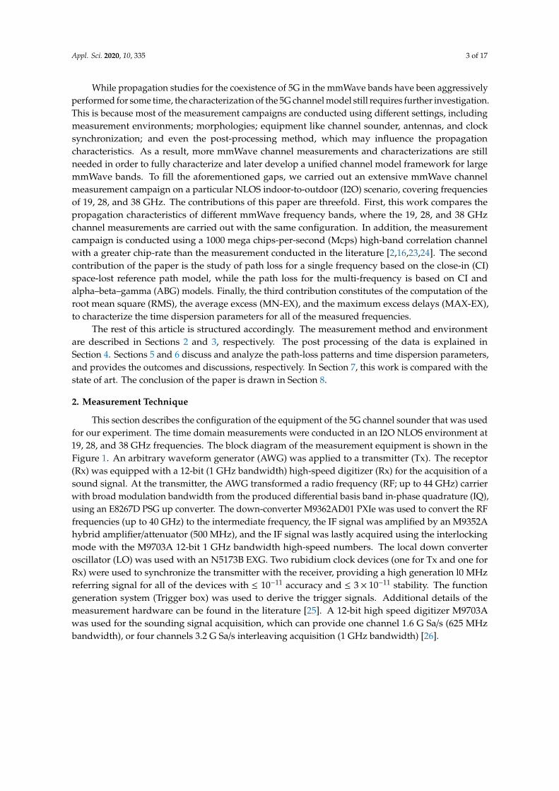
This section describes the configuration of the equipment of the 5G channel sounder that was usedfor our experiment. The time domain measurements were conducted in an I2O NLOS environment at19, 28, and 38 GHz frequencies. The block diagram of the measurement equipment is shown in theFigure 1. An arbitrary waveform generator (AWG) was applied to a transmitter (Tx). The receptor(Rx) was equipped with a 12-bit (1 GHz bandwidth) high-speed digitizer (Rx) for the acquisition of asound signal. At the transmitter, the AWG transformed a radio frequency (RF; up to 44 GHz) carrierwith broad modulation bandwidth from the produced differential basis band in-phase quadrature (IQ),using an E8267D PSG up converter. The down-converter M9362AD01 PXIe was used to convert the RFfrequencies (up to 40 GHz) to the intermediate frequency, the IF signal was amplified by an M9352Ahybrid amplifier/attenuator (500 MHz), and the IF signal was lastly acquired using the interlockingmode with the M9703A 12-bit 1 GHz bandwidth high-speed numbers. The local down converteroscillator (LO) was used with an N5173B EXG. Two rubidium clock devices (one for Tx and one forRx) were used to synchronize the transmitter with the receiver, providing a high generation l0 MHzreferring signal for all of the devices with ≤ 10−11 accuracy and ≤ 3 × 10−11 stability. The functiongeneration system (Trigger box) was used to derive the trigger signals. Additional details of themeasurement hardware can be found in the literature [25]. A 12-bit high speed digitizer M9703Awas used for the sounding signal acquisition, which can provide one channel 1.6 G Sa/s (625 MHzbandwidth), or four channels 3.2 G Sa/s interleaving acquisition (1 GHz bandwidth) [26].

Appl. Sci. 2020, 10, 335 4 of 17Appl. Sci. 2020, 10, x FOR PEER REVIEW 4 of 17

Figure 1. Block diagram of transmitter (Tx) and receptor (Rx) components for a 5G channel sounder.

The AWG yielded a 1-ns multipath resolution from a 1000 Mcps with sample rate of 7.2 GHz.

We used a signal generator (up-converter) to generate the center frequencies at 19, 28, and 38 GHz

with a transmitted power of 0 dBm. The signal was transmitted through a 11.6 dBi gain (39.9°/49.9°

azimuth/elevation half-power beamwidth (HPBW)), a 11.6 dBi gain (39.7°/49.7° azimuth/elevation

HPBW), and a 15.2 dBi gain (29.6°/29.7° azimuth/elevation HPBW) ETS-Lindgren horn antenna for

the 19, 28, and 38 GHz frequencies, respectively. At the receiver, an omnidirectional antenna (3 dBi

gain) with a relatively high gain power amplifier of 37 dB was used to collect the received signal.

3. Testbed of Experiment

The measurements were carried out at the Universiti Teknologi Malaysia, Kuala Lumpur (UTM-

KL) campus, in an indoor to outdoor setting at the Menara Tun Razak Building. The specific I2O

environment consisted of corridors surrounded by open and closed offices, conference rooms, and

meeting rooms. The floor plan and pictures of the measurement environment are shown in Figure

2a,c. The study environment contained corridors that had two open ends (to the north and the south),

as shown in Figure 2a. Figure 2b shows corridor A, where the the Tx antenna was placed, which was

open from the north side, and curved to corridor B from the other side. Corridor B, where the Rx was

placed, extended from corridor A, and was open from the south side, as shown by Figure 2c. Each of

the corridor’s walls were made up of a multitude of materials, including concrete, colored glass, and

wood. The floor was coated with glazed ceramic tiles, and ribbed metal was formed on the ceilings

of the hallways. The Tx antenna (1.7 m in height) was located in corridor A beside a concrete pillar.

The direction of the Tx horn antenna is indicated in Figure 2b (toward corridor A, in the direction of

the stairs and concrete pillar beside it). The Rx antenna (1.5 m in height) was an omnidirectional

antenna located in corridor B at the back of the Tx antenna, as shown in Figure 2c, which rendered

the environment completely NLOS. The first location of the Rx antenna was 3.7 m away from the Tx

horn antenna. The Rx was then moved by 1 m to the end of corridor B; the Tx–Rx separation distance

was then 13.5 m. The measurement configuration is shown in Figure 2a (left side).

Figure 1. Block diagram of transmitter (Tx) and receptor (Rx) components for a 5G channel sounder.

The AWG yielded a 1-ns multipath resolution from a 1000 Mcps with sample rate of 7.2 GHz.We used a signal generator (up-converter) to generate the center frequencies at 19, 28, and 38 GHzwith a transmitted power of 0 dBm. The signal was transmitted through a 11.6 dBi gain (39.9◦/49.9◦

azimuth/elevation half-power beamwidth (HPBW)), a 11.6 dBi gain (39.7◦/49.7◦ azimuth/elevationHPBW), and a 15.2 dBi gain (29.6◦/29.7◦ azimuth/elevation HPBW) ETS-Lindgren horn antenna for the19, 28, and 38 GHz frequencies, respectively. At the receiver, an omnidirectional antenna (3 dBi gain)with a relatively high gain power amplifier of 37 dB was used to collect the received signal.

3. Testbed of Experiment

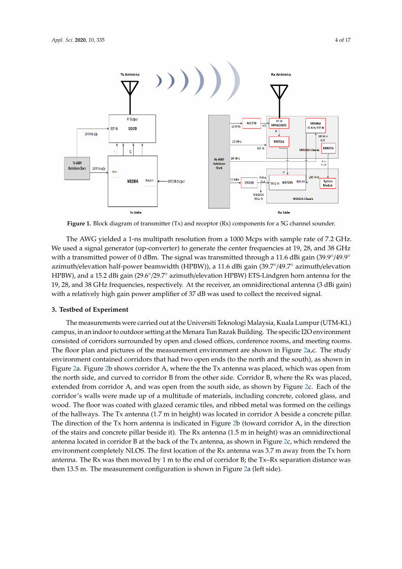
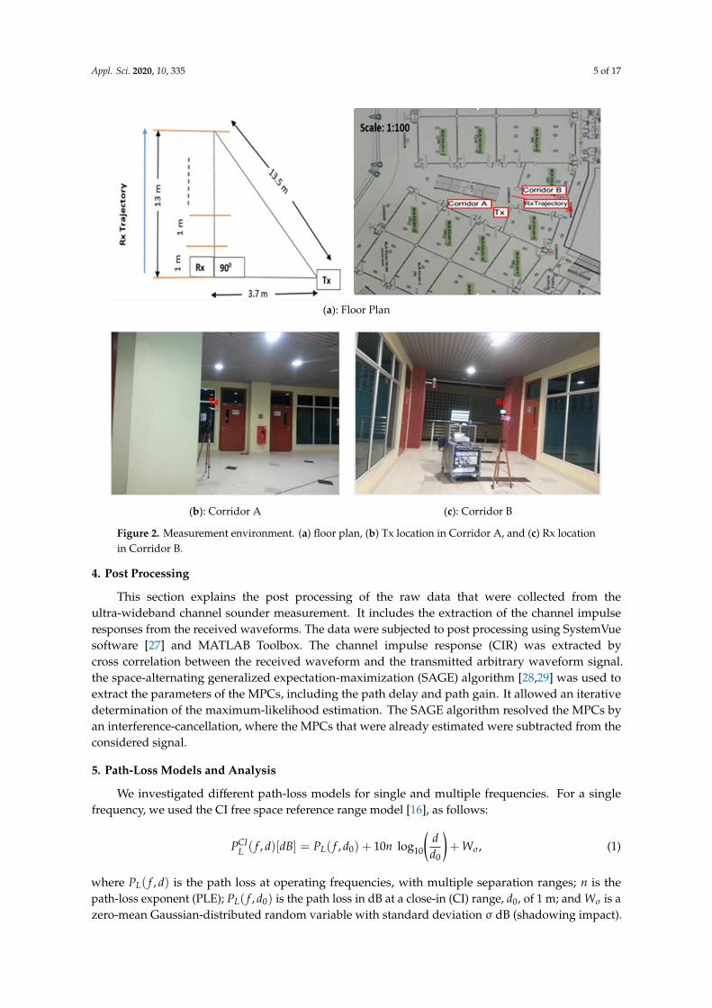
The measurements were carried out at the Universiti Teknologi Malaysia, Kuala Lumpur (UTM-KL)campus, in an indoor to outdoor setting at the Menara Tun Razak Building. The specific I2O environmentconsisted of corridors surrounded by open and closed offices, conference rooms, and meeting rooms.The floor plan and pictures of the measurement environment are shown in Figure 2a,c. The studyenvironment contained corridors that had two open ends (to the north and the south), as shown inFigure 2a. Figure 2b shows corridor A, where the the Tx antenna was placed, which was open fromthe north side, and curved to corridor B from the other side. Corridor B, where the Rx was placed,extended from corridor A, and was open from the south side, as shown by Figure 2c. Each of thecorridor’s walls were made up of a multitude of materials, including concrete, colored glass, andwood. The floor was coated with glazed ceramic tiles, and ribbed metal was formed on the ceilingsof the hallways. The Tx antenna (1.7 m in height) was located in corridor A beside a concrete pillar.The direction of the Tx horn antenna is indicated in Figure 2b (toward corridor A, in the directionof the stairs and concrete pillar beside it). The Rx antenna (1.5 m in height) was an omnidirectionalantenna located in corridor B at the back of the Tx antenna, as shown in Figure 2c, which rendered theenvironment completely NLOS. The first location of the Rx antenna was 3.7 m away from the Tx hornantenna. The Rx was then moved by 1 m to the end of corridor B; the Tx–Rx separation distance wasthen 13.5 m. The measurement configuration is shown in Figure 2a (left side).

Appl. Sci. 2020, 10, 335 5 of 17

Appl. Sci. 2020, 10, x FOR PEER REVIEW 5 of 17

(a): Floor Plan

(b): Corridor A (c): Corridor B

Figure 2. Measurement environment. (a) floor plan, (b) Tx location in Corridor A, and (c) Rx location

in Corridor B.

4. Post Processing

This section explains the post processing of the raw data that were collected from the ultra-

wideband channel sounder measurement. It includes the extraction of the channel impulse responses

from the received waveforms. The data were subjected to post processing using SystemVue software

[27] and MATLAB Toolbox. The channel impulse response (CIR) was extracted by cross correlation

between the received waveform and the transmitted arbitrary waveform signal. the space-alternating

generalized expectation-maximization (SAGE) algorithm [28,29] was used to extract the parameters

of the MPCs, including the path delay and path gain. It allowed an iterative determination of the

maximum-likelihood estimation. The SAGE algorithm resolved the MPCs by an interference-

cancellation, where the MPCs that were already estimated were subtracted from the considered

signal.

5. Path-Loss Models and Analysis

We investigated different path-loss models for single and multiple frequencies. For a single

frequency, we used the CI free space reference range model [16], as follows:

0 10

0

, [ ] ( , ) 10 logCI

L L

dP f d dB P f d n Wd

, (1)

where ,LP f d is the path loss at operating frequencies, with multiple separation ranges; n is the

path-loss exponent (PLE); 0( , )LP f d is the path loss in dB at a close-in (CI) range, d0, of 1 m; and W

is a zero-mean Gaussian-distributed random variable with standard deviation σ dB (shadowing

impact).

Figure 2. Measurement environment. (a) floor plan, (b) Tx location in Corridor A, and (c) Rx locationin Corridor B.

4. Post Processing

This section explains the post processing of the raw data that were collected from theultra-wideband channel sounder measurement. It includes the extraction of the channel impulseresponses from the received waveforms. The data were subjected to post processing using SystemVuesoftware [27] and MATLAB Toolbox. The channel impulse response (CIR) was extracted bycross correlation between the received waveform and the transmitted arbitrary waveform signal.the space-alternating generalized expectation-maximization (SAGE) algorithm [28,29] was used toextract the parameters of the MPCs, including the path delay and path gain. It allowed an iterativedetermination of the maximum-likelihood estimation. The SAGE algorithm resolved the MPCs byan interference-cancellation, where the MPCs that were already estimated were subtracted from theconsidered signal.

5. Path-Loss Models and Analysis

We investigated different path-loss models for single and multiple frequencies. For a singlefrequency, we used the CI free space reference range model [16], as follows:

PCIL ( f , d)[dB] = PL( f , d0) + 10n log10

(dd0

)+ Wσ, (1)

where PL( f , d) is the path loss at operating frequencies, with multiple separation ranges; n is thepath-loss exponent (PLE); PL( f , d0) is the path loss in dB at a close-in (CI) range, d0, of 1 m; and Wσ is azero-mean Gaussian-distributed random variable with standard deviation σ dB (shadowing impact).

Appl. Sci. 2020, 10, 335 6 of 17

The other model, with three parameters, is known as the ABG model. It includes a frequency-dependent term, γ; a distance-dependent term, α; and an optimization factor, β, to describe the pathloss at various frequencies [13,21,30]. The ABG model equation is given by the following [13]:

PLABG( f , d)[dB] = 10α log10

(dd0

)+ β+ 10γ log10

(f

fre f

)+ WABG

σ (2)

The minimum mean square error (MMSE) is the strategy by all of the parameters for the CI andABG path-loss models [16].

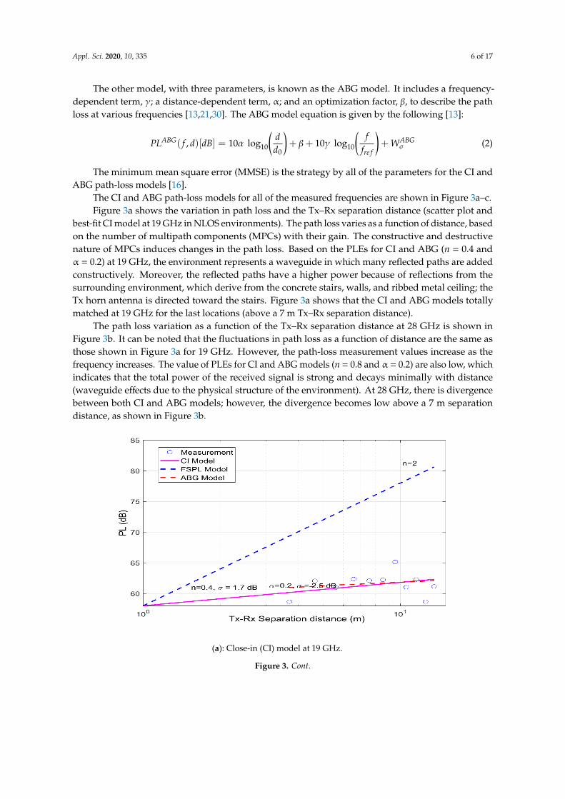
The CI and ABG path-loss models for all of the measured frequencies are shown in Figure 3a–c.Figure 3a shows the variation in path loss and the Tx–Rx separation distance (scatter plot and

best-fit CI model at 19 GHz in NLOS environments). The path loss varies as a function of distance, basedon the number of multipath components (MPCs) with their gain. The constructive and destructivenature of MPCs induces changes in the path loss. Based on the PLEs for CI and ABG (n = 0.4 andα = 0.2) at 19 GHz, the environment represents a waveguide in which many reflected paths are addedconstructively. Moreover, the reflected paths have a higher power because of reflections from thesurrounding environment, which derive from the concrete stairs, walls, and ribbed metal ceiling; theTx horn antenna is directed toward the stairs. Figure 3a shows that the CI and ABG models totallymatched at 19 GHz for the last locations (above a 7 m Tx–Rx separation distance).

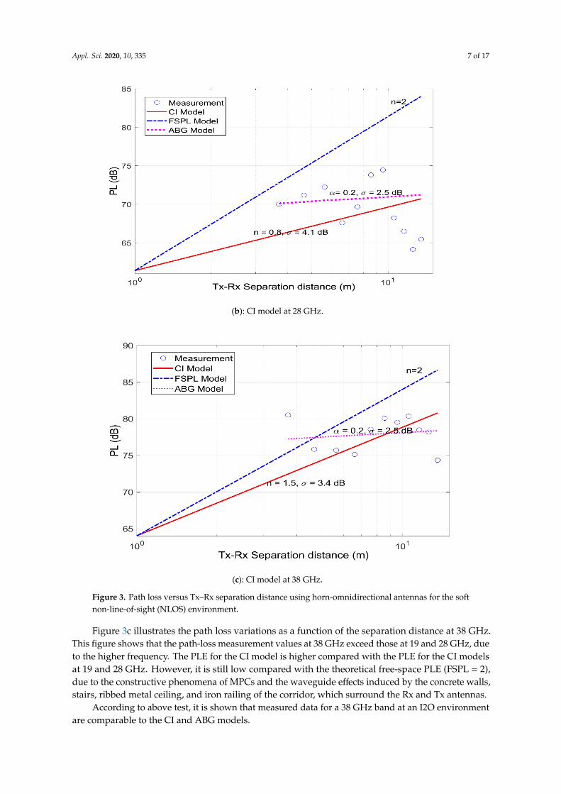
The path loss variation as a function of the Tx–Rx separation distance at 28 GHz is shown inFigure 3b. It can be noted that the fluctuations in path loss as a function of distance are the same asthose shown in Figure 3a for 19 GHz. However, the path-loss measurement values increase as thefrequency increases. The value of PLEs for CI and ABG models (n = 0.8 and α = 0.2) are also low, whichindicates that the total power of the received signal is strong and decays minimally with distance(waveguide effects due to the physical structure of the environment). At 28 GHz, there is divergencebetween both CI and ABG models; however, the divergence becomes low above a 7 m separationdistance, as shown in Figure 3b.

Appl. Sci. 2020, 10, x FOR PEER REVIEW 6 of 17

The other model, with three parameters, is known as the ABG model. It includes a frequency-

dependent term, ; a distance-dependent term, α; and an optimization factor, , to describe the

path loss at various frequencies [13,21,30]. The ABG model equation is given by the following [13]:

10 10

0

, 10 log 10 logABG ABG

ref

d fPL f d dB W

d f

(2)

The minimum mean square error (MMSE) is the strategy by all of the parameters for the CI and

ABG path-loss models [16].

The CI and ABG path-loss models for all of the measured frequencies are shown in Figure 3a–c.

Figure 3a shows the variation in path loss and the Tx–Rx separation distance (scatter plot and best-

fit CI model at 19 GHz in NLOS environments). The path loss varies as a function of distance, based

on the number of multipath components (MPCs) with their gain. The constructive and destructive

nature of MPCs induces changes in the path loss. Based on the PLEs for CI and ABG (n = 0.4 and α =

0.2) at 19 GHz, the environment represents a waveguide in which many reflected paths are added

constructively. Moreover, the reflected paths have a higher power because of reflections from the

surrounding environment, which derive from the concrete stairs, walls, and ribbed metal ceiling; the

Tx horn antenna is directed toward the stairs. Figure 3a shows that the CI and ABG models totally

matched at 19 GHz for the last locations (above a 7 m Tx–Rx separation distance).

(a): Close-in (CI) model at 19 GHz.

Figure 3. Cont.

Appl. Sci. 2020, 10, 335 7 of 17Appl. Sci. 2020, 10, x FOR PEER REVIEW 7 of 17

(b): CI model at 28 GHz.

(c): CI model at 38 GHz.

Figure 3. Path loss versus Tx–Rx separation distance using horn-omnidirectional antennas for the

soft non-line-of-sight (NLOS) environment.

The path loss variation as a function of the Tx–Rx separation distance at 28 GHz is shown in

Figure 3b. It can be noted that the fluctuations in path loss as a function of distance are the same as

those shown in Figure 3a for 19 GHz. However, the path-loss measurement values increase as the

frequency increases. The value of PLEs for CI and ABG models (n = 0.8 and α = 0.2) are also low,

which indicates that the total power of the received signal is strong and decays minimally with

distance (waveguide effects due to the physical structure of the environment). At 28 GHz, there is

divergence between both CI and ABG models; however, the divergence becomes low above a 7 m

separation distance, as shown in Figure 3b.

Figure 3. Path loss versus Tx–Rx separation distance using horn-omnidirectional antennas for the softnon-line-of-sight (NLOS) environment.

Figure 3c illustrates the path loss variations as a function of the separation distance at 38 GHz.This figure shows that the path-loss measurement values at 38 GHz exceed those at 19 and 28 GHz, dueto the higher frequency. The PLE for the CI model is higher compared with the PLE for the CI modelsat 19 and 28 GHz. However, it is still low compared with the theoretical free-space PLE (FSPL = 2),due to the constructive phenomena of MPCs and the waveguide effects induced by the concrete walls,stairs, ribbed metal ceiling, and iron railing of the corridor, which surround the Rx and Tx antennas.

According to above test, it is shown that measured data for a 38 GHz band at an I2O environmentare comparable to the CI and ABG models.

Appl. Sci. 2020, 10, 335 8 of 17

Here, the ABG model has a high deviation from the CI model at all locations of measurement.This implies that the ABG model is not recommended for a 38 GHz band at an I2O environment.Hence, when we lumped different frequencies from different bands (such as from 10, 20, and 30 GHz),it is recommended to use a CI model as well for the multi-frequency scheme.

Table 2 lists the parameter values for the CI and ABG path-loss models that are used to investigatethe multiple frequencies for the 5G channel propagation in this work. The CI path loss model ofEquation (1) can be used for multi-frequency schemes by putting all of the measurement data forall of the measured frequencies as one data set to find an overall PLE based on all of the potentialfrequencies measured. The PLE for the CI model in multi-frequencies is 0.9, which is calculated basedon the CI model in Equation (1) by using the MMSE approach under multiple regressions with threeindependent parameters—frequency, distance, and path loss.

Table 2. Multilateral path loss models 19, 28, and 38 GHz; CI; and alpha–beta–gamma (ABG)model parameters.

Model PLE σ

CI 0.9 5.2 dB

α β γ σABG 0.2 5.8 5.4 2.5 dB

It can be concluded that the high-frequency propagation channels in this specific I2O environmentexperience constructive interference from the ground, wall, and ceiling reflections. Furthermore, oneshould note the radical change in the path-loss values for all of the frequencies at the last two Rxlocations, due to reflections from the iron railing of the corridor. The PLE at the proposed frequenciesincreases with frequency. The PLE at 28 GHz is double that at 19 GHz, and the PLE at 38 GHz is abouttwice that at 28 GHz. This finding indicates that the PLE is frequency-dependent in this specific I2Oenvironment. The standard deviations of the CI path-loss model are 1.7, 4.2, and 3.4 dB, for 19, 28,and 38 GHz, respectively. The standard deviation of the CI model is low at 19 GHz, which indicatesthat the CI model has the best agreement with the measurement data. The standard deviation valuesat 28 and 38 GHz are more due to the rapid fluctuation of the received signal in some constructivemeasurement points. The rapid changes in the measured received signals are observed at 28 GHz, asshown in Figure 3b.

Based on the path-loss models’ parameters, as listed in Figure 3 and Table 2, we can conclude thatthe wireless signal can pass through the NLOS environment with a low signal power drop, using thehuge available bandwidth in high frequencies of 19, 28, and 38 GHz.

6. Time Dispersion Parameters and Analysis

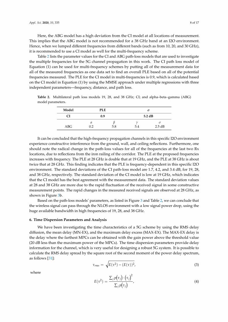
We have been investigating the time characteristics of a 5G scheme by using the RMS delaydiffusion, the mean delay (MN-EX), and the maximum delay excess (MAX-EX). The MAX-EX delay isthe delay where the farthest MPCs can be obtained with the gain power above the threshold value(20 dB less than the maximum power of the MPCs). The time dispersion parameters provide delayinformation for the channel, which is very useful for designing a robust 5G system. It is possible tocalculate the RMS delay spread by the square root of the second moment of the power delay spectrum,as follows [31]:

τrms =√

E(τ2) − (E(τ))2, (3)

where

E(τ2) =

∑j p

(τ j

)·

(τ j

)2∑j p

(τ j

) , (4)

Appl. Sci. 2020, 10, 335 9 of 17

and the MN-Ex is given as follows:

E(τ) =

∑j p

(τ j

)· τ j∑

j p(τ j

) , (5)

where p(τ j

)is the power of the multipath with delay τ j.

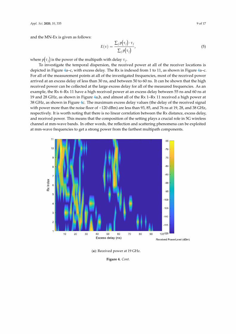
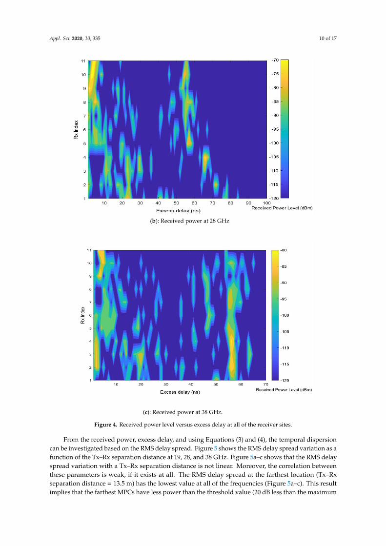
To investigate the temporal dispersion, the received power at all of the receiver locations isdepicted in Figure 4a–c, with excess delay. The Rx is indexed from 1 to 11, as shown in Figure 4a–c.For all of the measurement points at all of the investigated frequencies, most of the received powerarrived at an excess delay of less than 30 ns, and between 50 to 60 ns. It can be shown that the highreceived power can be collected at the large excess delay for all of the measured frequencies. As anexample, the Rx 6–Rx 11 have a high received power at an excess delay between 55 ns and 60 ns at19 and 28 GHz, as shown in Figure 4a,b, and almost all of the Rx 1–Rx 11 received a high power at38 GHz, as shown in Figure 4c. The maximum excess delay values (the delay of the received signalwith power more than the noise floor of −120 dBm) are less than 93, 85, and 76 ns at 19, 28, and 38 GHz,respectively. It is worth noting that there is no linear correlation between the Rx distance, excess delay,and received power. This means that the composition of the setting plays a crucial role in 5G wirelesschannel at mm-wave bands. In other words, the reflection and scattering phenomena can be exploitedat mm-wave frequencies to get a strong power from the farthest multipath components.

Appl. Sci. 2020, 10, x FOR PEER REVIEW 9 of 17

calculate the RMS delay spread by the square root of the second moment of the power delay

spectrum, as follows [31]:

2 2( ) ( ( ))rms E E , (3)

where

2

2( )j jj

jj

pE

p

, (4)

and the MN-Ex is given as follows:

( )

j jj

jj

pE

p

, (5)

where jp is the power of the multipath with delay j .

To investigate the temporal dispersion, the received power at all of the receiver locations is

depicted in Figure 4a–c, with excess delay. The Rx is indexed from 1 to 11, as shown in Figure 4a–c.

For all of the measurement points at all of the investigated frequencies, most of the received power

arrived at an excess delay of less than 30 ns, and between 50 to 60 ns. It can be shown that the high

received power can be collected at the large excess delay for all of the measured frequencies. As an

example, the Rx 6–Rx 11 have a high received power at an excess delay between 55 ns and 60 ns at 19

and 28 GHz, as shown in Figure 4a,b, and almost all of the Rx 1–Rx 11 received a high power at 38

GHz, as shown in Figure 4c. The maximum excess delay values (the delay of the received signal with

power more than the noise floor of −120 dBm) are less than 93, 85, and 76 ns at 19, 28, and 38 GHz,

respectively. It is worth noting that there is no linear correlation between the Rx distance, excess

delay, and received power. This means that the composition of the setting plays a crucial role in 5G

wireless channel at mm-wave bands. In other words, the reflection and scattering phenomena can be

exploited at mm-wave frequencies to get a strong power from the farthest multipath components.

(a): Received power at 19 GHz.

Figure 4. Cont.

Appl. Sci. 2020, 10, 335 10 of 17

Appl. Sci. 2020, 10, x FOR PEER REVIEW 10 of 17

(b): Received power at 28 GHz

(c): Received power at 38 GHz.

Figure 4. Received power level versus excess delay at all of the receiver sites.

From the received power, excess delay, and using Equations (3) and (4), the temporal dispersion

can be investigated based on the RMS delay spread. Figure 5 shows the RMS delay spread variation

as a function of the Tx–Rx separation distance at 19, 28, and 38 GHz. Figure 5a–c shows that the RMS

delay spread variation with a Tx–Rx separation distance is not linear. Moreover, the correlation

between these parameters is weak, if it exists at all. The RMS delay spread at the farthest location

(Tx–Rx separation distance = 13.5 m) has the lowest value at all of the frequencies (Figure 5a–c). This

result implies that the farthest MPCs have less power than the threshold value (20 dB less than the

Figure 4. Received power level versus excess delay at all of the receiver sites.

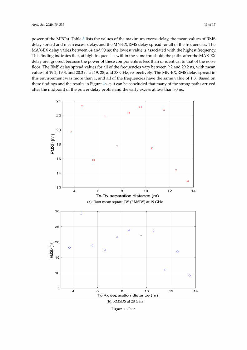
From the received power, excess delay, and using Equations (3) and (4), the temporal dispersioncan be investigated based on the RMS delay spread. Figure 5 shows the RMS delay spread variation as afunction of the Tx–Rx separation distance at 19, 28, and 38 GHz. Figure 5a–c shows that the RMS delayspread variation with a Tx–Rx separation distance is not linear. Moreover, the correlation betweenthese parameters is weak, if it exists at all. The RMS delay spread at the farthest location (Tx–Rxseparation distance = 13.5 m) has the lowest value at all of the frequencies (Figure 5a–c). This resultimplies that the farthest MPCs have less power than the threshold value (20 dB less than the maximum

Appl. Sci. 2020, 10, 335 11 of 17

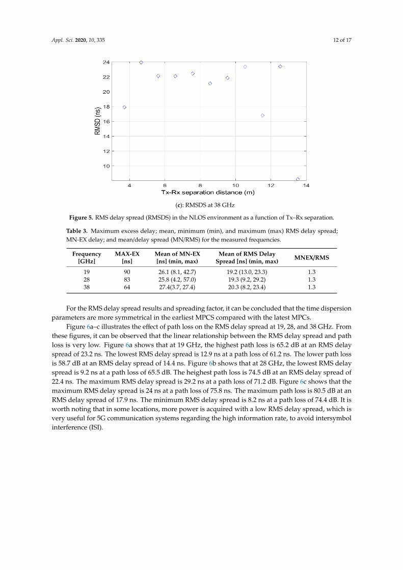
power of the MPCs). Table 3 lists the values of the maximum excess delay, the mean values of RMSdelay spread and mean excess delay, and the MN-EX/RMS delay spread for all of the frequencies. TheMAX-EX delay varies between 64 and 90 ns; the lowest value is associated with the highest frequency.This finding indicates that, at high frequencies within the same threshold, the paths after the MAX-EXdelay are ignored, because the power of these components is less than or identical to that of the noisefloor. The RMS delay spread values for all of the frequencies vary between 9.2 and 29.2 ns, with meanvalues of 19.2, 19.3, and 20.3 ns at 19, 28, and 38 GHz, respectively. The MN-EX/RMS delay spread inthis environment was more than 1, and all of the frequencies have the same value of 1.3. Based onthese findings and the results in Figure 4a–c, it can be concluded that many of the strong paths arrivedafter the midpoint of the power delay profile and the early excess at less than 30 ns.

Appl. Sci. 2020, 10, x FOR PEER REVIEW 11 of 17

maximum power of the MPCs). Table 3 lists the values of the maximum excess delay, the mean values

of RMS delay spread and mean excess delay, and the MN-EX/RMS delay spread for all of the

frequencies. The MAX-EX delay varies between 64 and 90 ns; the lowest value is associated with the

highest frequency. This finding indicates that, at high frequencies within the same threshold, the

paths after the MAX-EX delay are ignored, because the power of these components is less than or

identical to that of the noise floor. The RMS delay spread values for all of the frequencies vary

between 9.2 and 29.2 ns, with mean values of 19.2, 19.3, and 20.3 ns at 19, 28, and 38 GHz, respectively.

The MN-EX/RMS delay spread in this environment was more than 1, and all of the frequencies have

the same value of 1.3. Based on these findings and the results in Figure 4a–c, it can be concluded that

many of the strong paths arrived after the midpoint of the power delay profile and the early excess

at less than 30 ns.

(a): Root mean square DS (RMSDS) at 19 GHz

(b): RMSDS at 28 GHz

Figure 5. Cont.

Appl. Sci. 2020, 10, 335 12 of 17

Appl. Sci. 2020, 10, x FOR PEER REVIEW 12 of 17

(c): RMSDS at 38 GHz

Figure 5. RMS delay spread (RMSDS) in the NLOS environment as a function of Tx–Rx separation.

Table 3. Maximum excess delay; mean, minimum (min), and maximum (max) RMS delay spread;

MN-EX delay; and mean/delay spread (MN/RMS) for the measured frequencies.

Frequency

[GHz] MAX-EX [ns]

Mean of MN-EX [ns]

(min, max)

Mean of RMS Delay Spread

[ns] (min, max) MNEX/RMS

19 90 26.1 (8.1, 42.7) 19.2 (13.0, 23.3) 1.3

28 83 25.8 (4.2, 57.0) 19.3 (9.2, 29.2) 1.3

38 64 27.4(3.7, 27.4) 20.3 (8.2, 23.4) 1.3

For the RMS delay spread results and spreading factor, it can be concluded that the time

dispersion parameters are more symmetrical in the earliest MPCS compared with the latest MPCs.

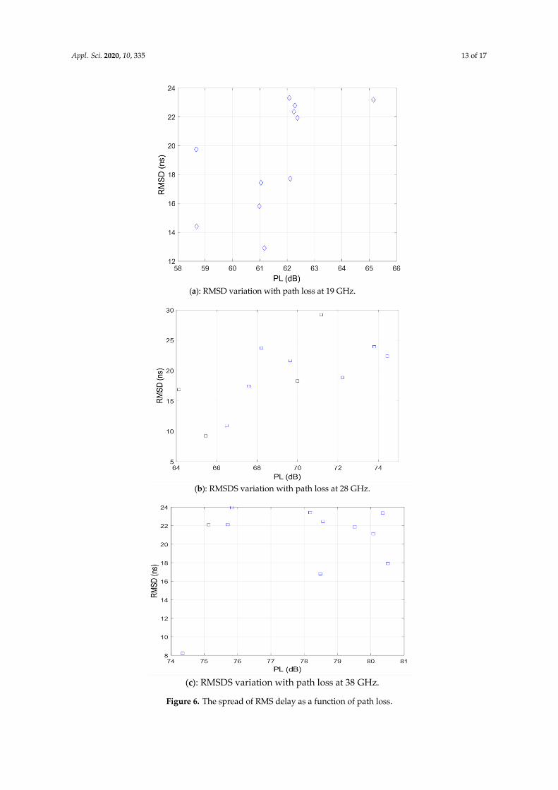
Figure 6a–c illustrates the effect of path loss on the RMS delay spread at 19, 28, and 38 GHz.

From these figures, it can be observed that the linear relationship between the RMS delay spread and

path loss is very low. Figure 6a shows that at 19 GHz, the highest path loss is 65.2 dB at an RMS delay

spread of 23.2 ns. The lowest RMS delay spread is 12.9 ns at a path loss of 61.2 ns. The lower path loss

is 58.7 dB at an RMS delay spread of 14.4 ns. Figure 6b shows that at 28 GHz, the lowest RMS delay

spread is 9.2 ns at a path loss of 65.5 dB. The heighest path loss is 74.5 dB at an RMS delay spread of

22.4 ns. The maximum RMS delay spread is 29.2 ns at a path loss of 71.2 dB. Figure 6c shows that the

maximum RMS delay spread is 24 ns at a path loss of 75.8 ns. The maximum path loss is 80.5 dB at

an RMS delay spread of 17.9 ns. The minimum RMS delay spread is 8.2 ns at a path loss of 74.4 dB. It

is worth noting that in some locations, more power is acquired with a low RMS delay spread, which

is very useful for 5G communication systems regarding the high information rate, to avoid

intersymbol interference (ISI).

Figure 5. RMS delay spread (RMSDS) in the NLOS environment as a function of Tx–Rx separation.

Table 3. Maximum excess delay; mean, minimum (min), and maximum (max) RMS delay spread;MN-EX delay; and mean/delay spread (MN/RMS) for the measured frequencies.

Frequency[GHz]

MAX-EX[ns]

Mean of MN-EX[ns] (min, max)

Mean of RMS DelaySpread [ns] (min, max) MNEX/RMS

19 90 26.1 (8.1, 42.7) 19.2 (13.0, 23.3) 1.328 83 25.8 (4.2, 57.0) 19.3 (9.2, 29.2) 1.338 64 27.4(3.7, 27.4) 20.3 (8.2, 23.4) 1.3

For the RMS delay spread results and spreading factor, it can be concluded that the time dispersionparameters are more symmetrical in the earliest MPCS compared with the latest MPCs.

Figure 6a–c illustrates the effect of path loss on the RMS delay spread at 19, 28, and 38 GHz. Fromthese figures, it can be observed that the linear relationship between the RMS delay spread and pathloss is very low. Figure 6a shows that at 19 GHz, the highest path loss is 65.2 dB at an RMS delayspread of 23.2 ns. The lowest RMS delay spread is 12.9 ns at a path loss of 61.2 ns. The lower path lossis 58.7 dB at an RMS delay spread of 14.4 ns. Figure 6b shows that at 28 GHz, the lowest RMS delayspread is 9.2 ns at a path loss of 65.5 dB. The heighest path loss is 74.5 dB at an RMS delay spread of22.4 ns. The maximum RMS delay spread is 29.2 ns at a path loss of 71.2 dB. Figure 6c shows that themaximum RMS delay spread is 24 ns at a path loss of 75.8 ns. The maximum path loss is 80.5 dB at anRMS delay spread of 17.9 ns. The minimum RMS delay spread is 8.2 ns at a path loss of 74.4 dB. It isworth noting that in some locations, more power is acquired with a low RMS delay spread, which isvery useful for 5G communication systems regarding the high information rate, to avoid intersymbolinterference (ISI).

Appl. Sci. 2020, 10, 335 13 of 17Appl. Sci. 2020, 10, x FOR PEER REVIEW 13 of 17

(a): RMSD variation with path loss at 19 GHz.

(b): RMSDS variation with path loss at 28 GHz.

(c): RMSDS variation with path loss at 38 GHz.

Figure 6. The spread of RMS delay as a function of path loss.

Figure 6. The spread of RMS delay as a function of path loss.

Appl. Sci. 2020, 10, 335 14 of 17

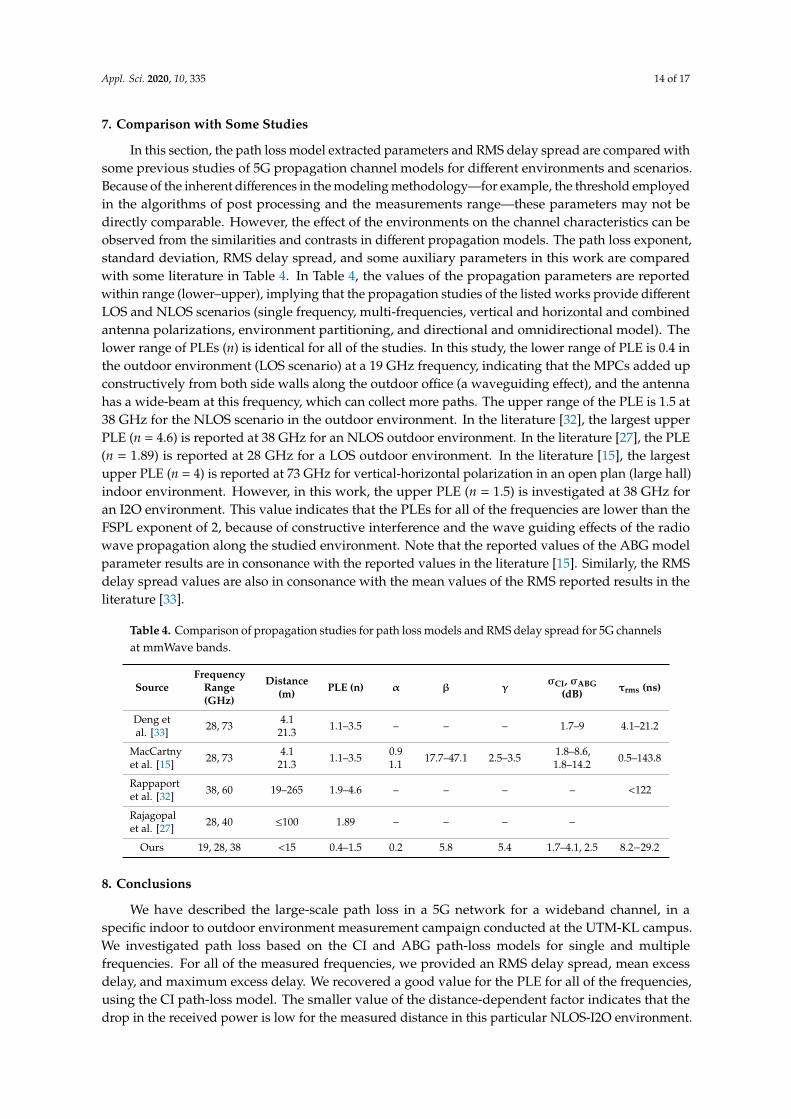
7. Comparison with Some Studies

In this section, the path loss model extracted parameters and RMS delay spread are compared withsome previous studies of 5G propagation channel models for different environments and scenarios.Because of the inherent differences in the modeling methodology—for example, the threshold employedin the algorithms of post processing and the measurements range—these parameters may not bedirectly comparable. However, the effect of the environments on the channel characteristics can beobserved from the similarities and contrasts in different propagation models. The path loss exponent,standard deviation, RMS delay spread, and some auxiliary parameters in this work are comparedwith some literature in Table 4. In Table 4, the values of the propagation parameters are reportedwithin range (lower–upper), implying that the propagation studies of the listed works provide differentLOS and NLOS scenarios (single frequency, multi-frequencies, vertical and horizontal and combinedantenna polarizations, environment partitioning, and directional and omnidirectional model). Thelower range of PLEs (n) is identical for all of the studies. In this study, the lower range of PLE is 0.4 inthe outdoor environment (LOS scenario) at a 19 GHz frequency, indicating that the MPCs added upconstructively from both side walls along the outdoor office (a waveguiding effect), and the antennahas a wide-beam at this frequency, which can collect more paths. The upper range of the PLE is 1.5 at38 GHz for the NLOS scenario in the outdoor environment. In the literature [32], the largest upperPLE (n = 4.6) is reported at 38 GHz for an NLOS outdoor environment. In the literature [27], the PLE(n = 1.89) is reported at 28 GHz for a LOS outdoor environment. In the literature [15], the largestupper PLE (n = 4) is reported at 73 GHz for vertical-horizontal polarization in an open plan (large hall)indoor environment. However, in this work, the upper PLE (n = 1.5) is investigated at 38 GHz foran I2O environment. This value indicates that the PLEs for all of the frequencies are lower than theFSPL exponent of 2, because of constructive interference and the wave guiding effects of the radiowave propagation along the studied environment. Note that the reported values of the ABG modelparameter results are in consonance with the reported values in the literature [15]. Similarly, the RMSdelay spread values are also in consonance with the mean values of the RMS reported results in theliterature [33].

Table 4. Comparison of propagation studies for path loss models and RMS delay spread for 5G channelsat mmWave bands.

SourceFrequency

Range(GHz)

Distance(m) PLE (n) α β γ

σCI, σABG(dB) τrms (ns)

Deng etal. [33] 28, 73 4.1

21.3 1.1–3.5 – – – 1.7–9 4.1–21.2

MacCartnyet al. [15] 28, 73 4.1

21.3 1.1–3.5 0.91.1 17.7–47.1 2.5–3.5 1.8–8.6,

1.8–14.2 0.5–143.8

Rappaportet al. [32] 38, 60 19–265 1.9–4.6 – – – – <122

Rajagopalet al. [27] 28, 40 ≤100 1.89 – – – –

Ours 19, 28, 38 <15 0.4–1.5 0.2 5.8 5.4 1.7–4.1, 2.5 8.2−29.2

8. Conclusions

We have described the large-scale path loss in a 5G network for a wideband channel, in aspecific indoor to outdoor environment measurement campaign conducted at the UTM-KL campus.We investigated path loss based on the CI and ABG path-loss models for single and multiplefrequencies. For all of the measured frequencies, we provided an RMS delay spread, mean excessdelay, and maximum excess delay. We recovered a good value for the PLE for all of the frequencies,using the CI path-loss model. The smaller value of the distance-dependent factor indicates that thedrop in the received power is low for the measured distance in this particular NLOS-I2O environment.

Appl. Sci. 2020, 10, 335 15 of 17

The PLE values are 0.4, 0.8, and 1.5 at measurement frequencies of 19, 28, and 38 GHz, respectively.The average RMS delay spread values are 19.2, 19.3, and 20.3 ns at 19, 28, and 38 GHz, respectively.The presented results showed that the path loss and RMS delay spread are not linearly dependent.The strong received signal can be detected at a low delay spread. Finally, our results from this study,together with other propagation studies in the literature, contributes to the development of a moreprecise and unified channel model framework for the studied mmWave bands of 19, 28, and 38 GHz.

Author Contributions: Conceptualization, A.M.A.-S., T.A.R., M.H.A. and T.A.-H.; methodology, A.M.A.-S., T.A.R.,M.H.A., T.A.-H., Y.F. and A.A.-M.; software, A.M.A.-S., T.A.R., M.H.A. and T.A.-H.; validation, A.M.A.-S., T.A.R.,M.H.A., T.A.-H., Y.F. and Y.A.A.-G.; formal analysis, A.M.A.-S., T.A.R. and T.A.-H.; investigation, A.M.A.-S., T.A.R.and T.A.-H.; resources A.M.A.-S., T.A.R. and T.A.-H.; data curation, A.M.A.-S., T.A.R., T.A.-H.; writing—originaldraft preparation, A.M.A.-S.; writing—review and editing, A.M.A.-S., T.A.R., M.H.A., T.A.-H., Y.F., Y.A.A.-G. andA.A.-M.; visualization, A.M.A.-S., T.A.R. and T.A.-H.; supervision, T.A.R.; project administration, A.M.A.-S., T.A.R.and T.A.-H.; funding acquisition, T.A.R. and T.A.-H. All authors have read and agreed to the published version ofthe manuscript.

Funding: This work was supported in part by H2020-MSCA-RISE-2015 under grant 690750. This research wasalso funded by the Research Management Centre (RMC), Universiti Teknologi Malaysia (UTM), under the WirelessCommunication Centre HICOE Grants. It was also supported by HICOE, Universiti Teknologi Malaysia (UTM)under Grant Q.J091300.23C9.00D96.

Conflicts of Interest: No conflict of interest is declared by the writers.

References

1. Pi, Z.; Khan, F. An introduction to millimeter-wave mobile broadband systems. IEEE Commun. Mag. 2011,49, 101–107. [CrossRef]

2. Rappaport, T.S.; MacCartney, G.R.; Samimi, M.K.; Sun, S. Wideband millimeter-wave propagationmeasurements and channel models for future wireless communication system design. IEEE Trans. Commun.2015, 63, 3029–3056. [CrossRef]

3. Smulders, P.F.M.; Wagemans, A.G. Wideband indoor radio propagation measurements at 58 GHz. Electron.Lett. 1992, 28, 1270. [CrossRef]

4. Geng, S.; Kivinen, J.; Zhao, X.; Vainikainen, P. Millimeter-wave propagation channel characterization forshort-range wireless communications. IEEE Trans. Veh. Technol. 2009, 58, 3–13. [CrossRef]

5. Ben-Dor, E.; Rappaport, T.S.; Qiao, Y.; Lauffenburger, S.J. Millimeter-wave 60 GHz outdoor and vehicle AOApropagation measurements using a broadband channel sounder. In Proceedings of the 2011 IEEE GlobalTelecommunications Conference—GLOBECOM 2011, Kathmandu, Nepal, 5–9 December 2011; pp. 1–6.

6. Shafi, M.; Molisch, A.F.; Smith, P.J.; Haustein, T.; Zhu, P.; De Silva, P.; Tufvesson, F.; Benjebbour, A.; Wunder, G.5G: A tutorial overview of standards, trials. IEEE J. Sel. Areas Commun. 2017, 35, 1201–1221. [CrossRef]

7. Al-Gumaei, Y.A.; Aslam, N.; Al-Samman, A.M.; Al-Hadhrami, T.; Noordin, K.; Fazea, Y. Non-cooperativepower control game in D2D underlying networks with variant system conditions. Electronics 2019, 8, 1113.[CrossRef]

8. ITU-R. World Radiocommunication Conference 2015—Provisional Final Acts. Available online: https://www.itu.int/dms_pub/itu-r/opb/act/R-ACT-WRC.11-2015-PDF-E.pdf (accessed on 29 November 2015).

9. Durgin, G.D.; Kukshya, V.; Rappaport, T.S. Wideband measurements of angle and delay dispersion foroutdoor and indoor peer-to-peer radio channels at 1920 MHz. IEEE Trans. Antennas Propag. 2003, 51, 936–944.[CrossRef]

10. Thomas, T.A.; Rybakowski, M.; Sun, S.; Rappaport, T.S.; Nguyen, H.; Kovács, I.Z. A prediction study ofpath loss models from 2–73.5 GHz in an urban-macro environment. In Proceedings of the 2016 IEEE 83rdVehicular Technology Conference (Spring VTC-2016), Nanjing, China, 15–18 May 2016.

11. MacCartney, G.R.; Rappaport, T.S. Rural macrocell path loss models for millimeter wave wirelesscommunications. IEEE J. Sel. Areas Commun. 2017, 35, 1663–1677. [CrossRef]

12. Sánchez, M.G.; Táboas, M.P.; Cid, E.L. Millimeter wave radio channel characterization for 5G vehicle-to-vehiclecommunications. Measurement 2017, 95, 223–229. [CrossRef]

13. Sun, S.; Rappaport, T.S.; Thomas, T.A.; Ghosh, A.; Nguyen, H.C.; Kovács, I.Z.; Rodriguez, I.; Koymen, O.;Partyka, A. Investigation of prediction accuracy, sensitivity, and parameter stability of large-scale propagationpath loss models for 5G wireless communications. IEEE Trans. Veh. Technol. 2016, 65, 2843–2860. [CrossRef]

Appl. Sci. 2020, 10, 335 16 of 17

14. Faruk, N.; Bello, O.W.; Sowande, O.A.; Onidare, S.O.; Muhammad, M.Y.; Ayeni, A.A. Large scale spectrumsurvey in rural and urban environments within the 50 MHz—6 GHz bands. Measurement 2016, 91, 228–238.[CrossRef]

15. Alvarez, A.; Valera, G.; Lobeira, M.; Torres, R.P.; Garcia, J.L. Ultra wideband channel model for indoorenvironments. J. Commun. Netw. 2003, 5, 309–318. [CrossRef]

16. Maccartney, G.R.; Rappaport, T.S.; Sun, S.; Deng, S. Indoor office wideband millimeter-wave propagationmeasurements and channel models at 28 and 73 GHz for ultra-dense 5G wireless networks. IEEE Access2015, 3, 2388–2424. [CrossRef]

17. Wang, Q.; Li, S.; Zhao, X.; Wang, M.; Sun, S. Wideband millimeter-wave channel characterization based onLOS measurements in an open office at 26GHz. In Proceedings of the 2016 IEEE 83rd Vehicular TechnologyConference (VTC Spring), Nanjing, China, 15–18 May 2016; pp. 1–5.

18. Hur, S.; Cho, Y.-J.; Lee, J.; Kang, No.; Park, J.; Benn, H. Synchronous channel sounder using horn antennaand indoor measurements on 28 GHz. In Proceedings of the 2014 IEEE International Black Sea Conferenceon Communications and Networking (BlackSeaCom), Odessa, Ukraine, 27–30 May 2014; pp. 83–87.

19. Al-Samman, A.M.; Rahman, T.A.; Azmi, M.H.; Hindia, M.N.; Khan, I.; Hanafi, E. Statistical modelling andcharacterization of experimental mm-wave indoor channels for future 5G wireless communication networks.PLoS ONE 2016, 11, e0163034. [CrossRef] [PubMed]

20. Azar, Y.; Wong, G.N.; Wang, K.; Mayzus, R.; Schulz, J.K.; Zhao, H.; Gutierrez, F.; Hwang, D.; Rappaport, T.S.28 GHz propagation measurements for outdoor cellular communications using steerable beam antennasin New York city. In Proceedings of the 2013 IEEE International Conference on Communications (ICC),Budapest, Hungary, 9–13 June 2013; pp. 5143–5147.

21. MacCartney, G.R.; Zhang, J.; Nie, S.; Rappaport, T.S. Path loss models for 5G millimeter wave propagationchannels in urban microcells. In Proceedings of the 2013 IEEE Global Communications Conference(GLOBECOM), Atlanta, GA, USA, 9–13 December 2013; pp. 3948–3953.

22. Sun, S.; MacCartney, G.R.; Rappaport, T.S. Millimeter-wave distance-dependent large-scale propagationmeasurements and path loss models for outdoor and indoor 5G systems. In Proceedings of the 2016 10thEuropean Conference Antennas Propagation (EuCAP 2016), Davos, Switzerland, 10–15 April 2016.

23. Kim, M.; Konishi, Y.; Chang, Y.; Takada, J.I. Large scale parameters and double-directional characterizationof indoor wideband radio multipath channels at 11 GHz. IEEE Trans. Antennas Propag. 2014, 62, 430–441.[CrossRef]

24. Kim, M.; Umeki, K.; Wangchuk, K.; Takada, J.; Sasaki, S. Polarimetric Mm-wave channel measurement andcharacterization in a small office. In Proceedings of the 2015 IEEE 26th Annual International Symposium onPersonal, Indoor, and Mobile Radio Communications (PIMRC), Hong Kong, China, 30 August–2 September2015; pp. 764–768.

25. Brochure, S. Keysight Technologies 5G Channel Sounding, Reference Solution. Available online: http://about.keysight.com/en/newsroom/pr/2015/30jul-em15109.shtml (accessed on 15 September 2015).

26. Oudin, H.; Wen, Z. mmWave MIMO channel sounding for 5G: Technical challenges and prototype system.In Proceedings of the 1st International Conference on 5G for Ubiquitous Connectivity, Levi, Finland,26–27 November 2014; pp. 192–197.

27. Rajagopal, S.; Abu-Surra, S.; Malmirchegini, M. Channel feasibility for outdoor non-line-of-sight mmWavemobile communication. In Proceedings of the 2012 IEEE Vehicular Technology Conference (VTC Fall),Quebec City, QC, Canada, 3–6 September 2012; pp. 1–6.

28. Yin, X.; He, Y.; Song, Z.; Kim, M.-D.; Chung, H.K. A sliding-correlator-based SAGE algorithm for Mm-wavewideband channel parameter estimation. In Proceedings of the 8th European Conference on Antennas andPropagation (EuCAP 2014), Hague, The Netherlands, 6–11 April 2014; pp. 625–629.

29. Fessler, J.A.; Hero, A.O. Space-alternating generalized expectation-maximization algorithm. IEEE Trans.Signal Process. 1994, 42, 2664–2677.

30. Piersanti, S.; Annoni, L.A.; Cassioli, D. Millimeter waves channel measurements and path loss models.In Proceedings of the 2012 IEEE International Conference on Communications (ICC), Ottawa, ON, Canada,10–15 June 2012; pp. 4552–4556.

31. Rappaport, T.S. Wireless Communications Principles and Practice, 2nd ed.; Prentice Hall: Upper Saddle River,NJ, USA, 2002.

Appl. Sci. 2020, 10, 335 17 of 17

32. Rappaport, T.S.; Ben-Dor, E.; Murdock, J.N.; Qiao, Y. 38 GHz and 60 GHz angle-dependent propagation forcellular & peer-to-peer wireless communications. In Proceedings of the IEEE International Conference onCommunications, Ottawa, ON, Canada, 10–15 June 2012; pp. 4568–4573.

33. Deng, S.; Samimi, M.K.; Rappaport, T.S. 28 GHz and 73 GHz millimeter-wave indoor propagationmeasurements and path loss models. In Proceedings of the 2015 IEEE International Conference onCommunication Workshop (ICCW), London, UK, 8–12 June 2015; pp. 1244–1250.

© 2020 by the authors. Licensee MDPI, Basel, Switzerland. This article is an open accessarticle distributed under the terms and conditions of the Creative Commons Attribution(CC BY) license (http://creativecommons.org/licenses/by/4.0/).