Date post: | 27-May-2018 |
Category: |
Documents |
Upload: | hoangquynh |
View: | 247 times |
Download: | 0 times |
UNIVERSITE DE MONTREAL
MIMO COMMUNICATION SYSTEMS WITH RECONFIGURABLE ANTENNAS
VIDA VAKILIAN
DEPARTEMENT DE GENIE ELECTRIQUE
ECOLE POLYTECHNIQUE DE MONTREAL
THESE PRESENTEE EN VUE DE L’OBTENTION
DU DIPLOME DE PHILOSOPHIÆ DOCTOR
(GENIE ELECTRIQUE)
JUIN 2014
c© Vida Vakilian, 2014.
UNIVERSITE DE MONTREAL
ECOLE POLYTECHNIQUE DE MONTREAL
Cette these intitulee :
MIMO COMMUNICATION SYSTEMS WITH RECONFIGURABLE ANTENNAS
presentee par : VAKILIAN Vida
en vue de l’obtention du diplome de : Philosophiæ Doctor
a ete dument acceptee par le jury d’examen constitue de :
M. WU Ke, Ph.D., president
M. FRIGON Jean-Francois, Ph.D., membre et directeur de recherche
M. ROY Sebastien, Ph.D., membre et codirecteur de recherche
M. CARDINAL Christian, Ph.D., membre
M. SHAYAN Yousef R., Ph.D., membre
iii
ACKNOWLEDGEMENTS
First and foremost, I would like to express my sincere gratitude to my advisor Prof. Jean-
Francois Frigon for his support, guidance and depth of knowledge. His insightful comments
and suggestions have helped me to advance my research and improve the quality of this
dissertation. I would also like to thank my co-adviser Prof. Sebastien Roy for his valuable
feedback and advice throughout this research. My sincere thanks goes to my supervisors at
Alcatel-Lucent, Dr. Thorsten Wild and Dr. Stephan Ten Brink who gave me an opportunity
to have my internship with their research group and work on diverse exciting projects. I
also thank Prof. Zhi Ding, my internship supervisor at University of California, Davis. I
especially thank Dr. Shahrokh Nayeb Nazar and Dr. Afshin Haghighat for their support,
guidance and supervision during my work at InterDigital Communications. I would also like
to express gratitude to the members of my dissertation committee, Prof. Ke Wu, Prof. Yousef
R. Shayan and Prof. Christian Cardinal for their valuable time and constructive feedback.
I have also learned from my interactions with some very talented friends, Diego Perea-
Vega, Arash Azarfar, Mohammad Torabi, Ali Torabi, Xingliang Li and Mohamed Jihed Gafsi.
I am also forever indebted to my parents for their love and support. They have given me eve-
rything they could, and they have been encouraging me to make my own decisions throughout
my life. Lastly, and most importantly, I would like to thank my husband and best friend,
Reza Abdolee. He was always there cheering me up and stood by me through the up’s and
down’s of my life.
Here, I acknowledge that this research would not have been possible without: a) research
assistantship from Prof. Jean-Francois Frigon via Fonds Quebecois de la Recherche sur la
Nature et les Technologies (FQRNT), b) Supplementary scholarships from Regroupement
Strategique en Microsysteme du Quebec (ReSMiQ) c) An internship award from Centre de
Recherche en Electronique Radiofrequence (CREER), and d) An international Research In-
ternship in Science and Engineering (RISE) award from German Academic Exchange Service
(DAAD). I would like to express my gratitude to all those individuals and agencies for their
support.
iv
RESUME
Les antennes reconfigurables sont capables d’ajuster dynamiquement les caracteristiques
de leur diagramme de rayonnement, par exemple, la forme, la direction et la polarisation,
en reponse aux conditions environnementales et exigences du systeme. Ces antennes peuvent
aussi etre utilisees en conjonction avec des systeme a entrees multiples sorties multiples
(MIMO) pour ameliorer davantage la capacite et la fiabilite des systemes sans fil. Cette these
etudie certains des problemes dans les systemes sans fil equipes d’antennes reconfigurables et
propose des solutions pour ameliorer la performance du systeme.
Dans les systemes sans fil utilisant des antennes reconfigurables, la performance attei-
gnable par le systeme depend fortement de la connaissance de la direction d’arrivee (DoA)
des signaux souhaites et des interferences. Dans la premiere partie de cette these, nous propo-
sons un nouvel algorithme d’estimation de la DoA pour les systeme a entree simple et sortie
simple (SISO) qui possedent un element d’antenne reconfigurable au niveau du recepteur.
Contrairement a un systeme utilisant un reseau d’antennes conventionnelles a diagramme de
rayonnement fixe, ou la DoA est estimee en utilisant les signaux recus par plusieurs elements,
dans le reseau d’antennes avec l’algorithme propose, la DoA est estimee en utilisant des si-
gnaux recus d’un element d’antenne unique pendant qu’il balai un ensemble de configurations
de diagramme de rayonnement. Nous etudions aussi l’impact des differentes caracteristiques
des diagrammes de rayonnement utilises, tels que la largeur du faisceau de l’antenne et le
nombre d’etapes de numerisation, sur l’exactitude de la DoA estimee.
Dans la deuxieme partie de cette these, nous proposons un systeme de MIMO faible com-
plexite employant des antennes reconfigurables sur les canaux selectifs en frequence pour
attenuer les effets de trajets multiples et donc eliminer l’interference entre symboles sans
utiliser la technique de modulation multiplexage orthogonale frequentiel (OFDM). Nous etu-
dions aussi l’impact de la propagation et de l’antenne angulaire largeur de faisceau sur la
performance du systeme propose et faire la comparaison avec la performance du systeme
MIMO-OFDM.
Dans la troisieme partie de cette these, nous fournissons des outils analytiques pour analy-
ser la performance des systemes sans fil MIMO equipes d’antennes reconfigurables au niveau
du recepteur. Nous derivons d’abord des expressions analytiques pour le calcul de la matrice
de covariance des coefficients des signaux recus empietant sur un reseau d’antennes reconfi-
gurables en tenant compte de plusieurs caracteristiques de l’antenne tels que la largeur du
faisceau, l’espacement d’antenne, l’angle de pointage ainsi que le gain de l’antenne. Dans cette
partie, nous considerons un recepteur MIMO reconfigurable ou le diagramme de rayonnement
v
de chaque element d’antenne dans le reseau peut avoir des caracteristiques differentes. Nous
etudions egalement la capacite d’un systeme MIMO reconfigurable en utilisant les expressions
analytiques derivees.
Dans la derniere partie de la these, nous proposons une nouvelle technique de codage du
bloc tri-dimensionelle pour les systemes reconfigurable MIMO-OFDM qui tirent partie des
caracteristiques de l’antenne reconfigurables pour ameliorer la diversite de systeme sans fil
et de la performance. Le code en bloc propose est capable d’extraire de multiple gains de
diversite, y compris spatiale, en frequence et de diagramme de rayonnement. Afin d’obte-
nir la diversite de diagramme de rayonnement, nous configurons chaque element d’antenne
d’emission pour basculer independamment son diagramme de rayonnement dans les direc-
tions selectionnees en fonction de differents criteres d’optimisation ; par exemple, la reduction
de la correlation entre les differents etats de rayonnement ou l’augmentation de la puissance
recue. Le code en bloc quasi orthogonale propose, qui est de taux unitaire et qui beneficie de
trois types de diversite, ameliore sensiblement les performances d’erreur binaire (BER) des
systemes MIMO.
vi
ABSTRACT
Reconfigurable antennas are able to dynamically adjust their radiation pattern charac-
teristics, e.g., shape, direction and polarization, in response to environmental conditions
and system requirements. These antennas can be used in conjunction with multiple-input
multiple-output (MIMO) systems to further enhance the capacity and reliability of wireless
networks. This dissertation studies some of the issues in wireless cellular systems equipped
with reconfigurable antennas and offer solutions to enhance their performance.
In wireless systems employing reconfigurable antennas, the attainable performance im-
provement highly depends on the knowledge of direction-of-arrival (DoA) of the desired
source signals and that of the interferences. In the first part of this dissertation, we pro-
pose a novel DoA estimation algorithm for single-input single-output (SISO) system with a
reconfigurable antenna element at the receiver. Unlike a conventional antenna array system
with fixed radiation pattern where the DoA is estimated using the signals received by mul-
tiple elements, in the proposed algorithm, we estimate the DoA using signals collected from
a set of radiation pattern states also called scanning steps. We, in addition, investigate the
impact of different radiation pattern characteristics such as antenna beamwidth and number
of scanning steps on the accuracy of the estimated DoA.
In the second part of this dissertation, we propose a low-complexity MIMO system em-
ploying reconfigurable antennas over the frequency-selective channels to mitigate multipath
effects and therefore remove inter symbol interference without using orthogonal frequency-
division multiplexing (OFDM) modulation. We study the impact of angular spread and
antenna beamwidth on the performance of the proposed system and make comparisons with
that of MIMO-OFDM system equipped with omnidirectional antennas.
In the third part of this dissertation, we provide an analytical tool to analyze the per-
formance of MIMO wireless systems equipped with reconfigurable antennas at the receiver.
We first derive analytical expressions for computing the covariance matrix coefficients of the
received signals impinging on a reconfigurable antenna array by taking into account several
antenna characteristics such as beamwidth, antenna spacing, antenna pointing angle, and
antenna gain. In this part, we consider a reconfigurable MIMO receiver where the radiation
pattern of each antenna element in the array can have different characteristics. We, addi-
tionally, study the capacity of a reconfigurable MIMO system using the derived analytical
expressions.
In the last part of the dissertation, we propose a novel three dimensional block coding tech-
nique for reconfigurable MIMO-OFDM systems which takes advantage of the reconfigurable
vii
antenna features to enhance the wireless system diversity and performance. The proposed
block code achieves multiple diversity gains, including, spatial, frequency, and state by trans-
mitting a block code over multiple transmit antennas, OFDM tones, and radiation states.
To obtain the state diversity, we configure each transmit antenna to independently switch
its radiation pattern to a direction that can be selected according to different optimization
criteria, e.g., minimization of the correlation among different radiation states. The proposed
code is full rate and benefits from three types of diversity, which substanttially improves the
bit-error-rate (BER) performance of the MIMO systems.
viii
TABLE OF CONTENTS
ACKNOWLEDGEMENTS . . . . . . . . . . . . . . . . . . . . . . . . . . . . . . . . . iii
RESUME . . . . . . . . . . . . . . . . . . . . . . . . . . . . . . . . . . . . . . . . . . . iv
ABSTRACT . . . . . . . . . . . . . . . . . . . . . . . . . . . . . . . . . . . . . . . . . vi
TABLE OF CONTENTS . . . . . . . . . . . . . . . . . . . . . . . . . . . . . . . . . . viii
LIST OF TABLES . . . . . . . . . . . . . . . . . . . . . . . . . . . . . . . . . . . . . . xi
LIST OF FIGURES . . . . . . . . . . . . . . . . . . . . . . . . . . . . . . . . . . . . . xii
LIST OF APPENDICES . . . . . . . . . . . . . . . . . . . . . . . . . . . . . . . . . . . xv
LIST OF ACRONYMS . . . . . . . . . . . . . . . . . . . . . . . . . . . . . . . . . . . xvi
NOTATIONS . . . . . . . . . . . . . . . . . . . . . . . . . . . . . . . . . . . . . . . . .xviii
CHAPTER 1 Introduction . . . . . . . . . . . . . . . . . . . . . . . . . . . . . . . . . 1
1.1 Objectives and Contributions . . . . . . . . . . . . . . . . . . . . . . . . . . . 1
1.2 Outline of the Dissertation . . . . . . . . . . . . . . . . . . . . . . . . . . . . . 4
CHAPTER 2 Literature review . . . . . . . . . . . . . . . . . . . . . . . . . . . . . . 6
2.1 Related Works . . . . . . . . . . . . . . . . . . . . . . . . . . . . . . . . . . . . 6
2.2 Background Study . . . . . . . . . . . . . . . . . . . . . . . . . . . . . . . . . 8
2.2.1 Fading . . . . . . . . . . . . . . . . . . . . . . . . . . . . . . . . . . . . 8
2.2.2 Diversity Gain . . . . . . . . . . . . . . . . . . . . . . . . . . . . . . . . 9
2.2.3 Coding Techniques for MIMO Systems . . . . . . . . . . . . . . . . . . 9
2.2.4 Reconfigurable MIMO Systems . . . . . . . . . . . . . . . . . . . . . . 11
2.2.5 Coding Techniques for Reconfigurable MIMO Systems . . . . . . . . . 11
CHAPTER 3 DoA Estimation for Reconfigurable Antenna Systems . . . . . . . . . . 14
3.1 Signal Model . . . . . . . . . . . . . . . . . . . . . . . . . . . . . . . . . . . . 15
3.2 DoA Algorithm for a Single Reconfigurable Antenna Element . . . . . . . . . . 17
3.2.1 Radiation Pattern Scan-MUSIC Algorithm . . . . . . . . . . . . . . . . 17
3.2.2 Power Pattern Cross-Correlation Approach . . . . . . . . . . . . . . . . 19
ix
3.2.3 Numerical Results . . . . . . . . . . . . . . . . . . . . . . . . . . . . . 20
3.3 Impact of DoA Estimation Errors on the BER Performance of Reconfigurable
SISO Systems . . . . . . . . . . . . . . . . . . . . . . . . . . . . . . . . . . . . 23
3.3.1 BER Analysis for a Reconfigurable SISO System . . . . . . . . . . . . . 24
3.3.2 BER Analysis for a Reconfigurable SISO System with DoA Estimation
Error . . . . . . . . . . . . . . . . . . . . . . . . . . . . . . . . . . . . . 26
3.3.3 Simulation Results . . . . . . . . . . . . . . . . . . . . . . . . . . . . . 27
3.4 Experimental Study of DoA Estimation Using Reconfigurable Antennas . . . . 30
3.4.1 Measurement Setup . . . . . . . . . . . . . . . . . . . . . . . . . . . . . 30
3.4.2 Experimental Results . . . . . . . . . . . . . . . . . . . . . . . . . . . . 32
3.5 Conclusion . . . . . . . . . . . . . . . . . . . . . . . . . . . . . . . . . . . . . . 34
CHAPTER 4 Performance Evaluation of Reconfigurable MIMO Systems in Spatially
Correlated Frequency-Selective Fading Channels . . . . . . . . . . . . . . . . . . . . 35
4.1 Spatial Channel Model . . . . . . . . . . . . . . . . . . . . . . . . . . . . . . . 36
4.2 Space-Time-State coded RE-MIMO System in Frequency-Selective Channels . 37
4.3 Space-Time Coded MIMO-OFDM System . . . . . . . . . . . . . . . . . . . . 41
4.4 Simulation Results . . . . . . . . . . . . . . . . . . . . . . . . . . . . . . . . . 43
4.5 Conclusion . . . . . . . . . . . . . . . . . . . . . . . . . . . . . . . . . . . . . . 45
CHAPTER 5 Covariance Matrix and Capacity Evaluation of Reconfigurable Antenna
Array Systems . . . . . . . . . . . . . . . . . . . . . . . . . . . . . . . . . . . . . . 46
5.1 Modeling and Problem Formulation . . . . . . . . . . . . . . . . . . . . . . . . 47
5.2 Closed-Form Expressions for Covariance Matrix Coefficients . . . . . . . . . . 49
5.2.1 Computer Experiments . . . . . . . . . . . . . . . . . . . . . . . . . . . 58
5.3 Reconfigurable MIMO Channel Capacity . . . . . . . . . . . . . . . . . . . . . 60
5.3.1 Computer Experiments . . . . . . . . . . . . . . . . . . . . . . . . . . . 62
5.4 Conclusion . . . . . . . . . . . . . . . . . . . . . . . . . . . . . . . . . . . . . . 65
CHAPTER 6 Full-Diversity Full-Rate Space-Frequency-State Block Codes for Reconfi-
gurable MIMO Systems . . . . . . . . . . . . . . . . . . . . . . . . . . . . . . . . . 67
6.1 System Model for Reconfigurable MIMO-OFDM Systems . . . . . . . . . . . . 68
6.2 Quasi-Orthogonal Space-Frequency Block Codes . . . . . . . . . . . . . . . . . 70
6.3 Quasi-Orthogonal Space-Frequency-State Block Codes . . . . . . . . . . . . . . 71
6.3.1 Code Structure . . . . . . . . . . . . . . . . . . . . . . . . . . . . . . . 72
6.4 Example of a Space-Frequency-State Block Code . . . . . . . . . . . . . . . . . 73
6.5 Error Rate Performance for Space-Frequency-State Block Codes . . . . . . . . 74
x
6.6 QOSFS Code Design Criteria . . . . . . . . . . . . . . . . . . . . . . . . . . . 75
6.6.1 Maximum Diversity Order . . . . . . . . . . . . . . . . . . . . . . . . . 75
6.6.2 Coding Gain . . . . . . . . . . . . . . . . . . . . . . . . . . . . . . . . . 78
6.7 Optimal Rotation Angles . . . . . . . . . . . . . . . . . . . . . . . . . . . . . . 78
6.8 Simulation Results . . . . . . . . . . . . . . . . . . . . . . . . . . . . . . . . . 84
6.8.1 2-Ray Channel Model . . . . . . . . . . . . . . . . . . . . . . . . . . . 85
6.8.2 Clustered Channel Model . . . . . . . . . . . . . . . . . . . . . . . . . 88
6.9 Conclusion . . . . . . . . . . . . . . . . . . . . . . . . . . . . . . . . . . . . . . 91
CHAPTER 7 Conclusion . . . . . . . . . . . . . . . . . . . . . . . . . . . . . . . . . . 93
7.1 Summary . . . . . . . . . . . . . . . . . . . . . . . . . . . . . . . . . . . . . . 93
7.2 Future Works . . . . . . . . . . . . . . . . . . . . . . . . . . . . . . . . . . . . 94
Bibliography . . . . . . . . . . . . . . . . . . . . . . . . . . . . . . . . . . . . . . . . . 96
Appendices . . . . . . . . . . . . . . . . . . . . . . . . . . . . . . . . . . . . . . . . . . 104
xi
LIST OF TABLES
Table 3.1 Experimental parameters . . . . . . . . . . . . . . . . . . . . . . . . . . 30
Table 3.2 Different cases for radiation states . . . . . . . . . . . . . . . . . . . . . . 31
Table 4.1 Simulation parameters for the proposed RE-MIMO and MIMO-OFDM
systems . . . . . . . . . . . . . . . . . . . . . . . . . . . . . . . . . . . 44
xii
LIST OF FIGURES
Figure 1.1 Flow of the main works of this dissertation . . . . . . . . . . . . . . . . 2
Figure 3.1 Single reconfigurable antenna with P radiation pattern states . . . . . 16
Figure 3.2 Radiation pattern of a reconfigurable antenna for four different radia-
tion state . . . . . . . . . . . . . . . . . . . . . . . . . . . . . . . . . . 18
Figure 3.3 RPS-MUSIC spectrum for two sources with θ1 = −25 and θ2 = 35. . 20
Figure 3.4 RMSE of RPS-MUSIC for different number of snapshots . . . . . . . . 21
Figure 3.5 RMSE of RPS-MUSIC versus different number of radiation states for
different number of snapshots . . . . . . . . . . . . . . . . . . . . . . . 21
Figure 3.6 RMSE of RPS-MUSIC for different number of radiation states and
same amount of information for all the states . . . . . . . . . . . . . . 22
Figure 3.7 Power spectrum for one sources with θ1 = 10 . . . . . . . . . . . . . . 23
Figure 3.8 System model for the RE-SISO system with a reconfigurable antenna
at the receiver . . . . . . . . . . . . . . . . . . . . . . . . . . . . . . . . 25
Figure 3.9 Effect of DoA estimation errors on the average bit error rate . . . . . . 27
Figure 3.10 Average bit error rate performance of the RE-SISO system versus an-
gular spread for different amounts of DoA estimation errors at SNR=
20dB . . . . . . . . . . . . . . . . . . . . . . . . . . . . . . . . . . . . . 28
Figure 3.11 Effect of DoA estimation errors on the average bit error rate for different
values of angular spread at SNR= 20dB (AS) . . . . . . . . . . . . . . 29
Figure 3.12 Effect of antenna beamwidth on the average bit error rate for different
amounts of DoA estimation errors . . . . . . . . . . . . . . . . . . . . . 29
Figure 3.13 The measurement setup for one-source DoA estimation in an anechoic
chamber. . . . . . . . . . . . . . . . . . . . . . . . . . . . . . . . . . . . 31
Figure 3.14 Power spectrum for DoA of 0 with P = 2
. . . . . . . . . . . . . . . . . . . . . . . . . . . . . . . . . . . . . . . . 32
Figure 3.15 Power spectrum for DoA of 30 with P = 2 . . . . . . . . . . . . . . . . . . . 33
Figure 3.16 Power spectrum for DoA of 30 with P = 4 . . . . . . . . . . . . . . . . . . . 33
Figure 4.1 RE-MIMO system with Mt = 2, Mr = 2 and L = 2 clusters. . . . . . . 38
Figure 4.2 MIMO-OFDM system with Mt = 2, Mr = 2 and L = 2 clusters. . . . . 41
Figure 4.3 Average BER vs. SNR for RE-MIMO and MIMO-OFDM systems with
Mt = 2, Mr = 2, L = 2, and angular spread of 10. . . . . . . . . . . . 44
Figure 4.4 Average BER vs. received angular spread for RE-MIMO and MIMO-
OFDM systems with Mt = 2, Mr = 2, and L = 2 clusters. . . . . . . . 45
xiii
Figure 5.1 PAS and the reconfigurable antenna radiation patterns . . . . . . . . . 49
Figure 5.2 Plot of Bessel function of the first kind, J2k(Dr) at the top for integer
orders k = 1, 2, 3, 4, 5, 6 and J2k+1 at the bottom for integer orders k
= 0, 1, 2, 3, 4, 5. . . . . . . . . . . . . . . . . . . . . . . . . . . . . . . 57
Figure 5.3 Convergence of correlation coefficient as a function of number of terms
in summation . . . . . . . . . . . . . . . . . . . . . . . . . . . . . . . . 57
Figure 5.4 Covariance coefficient with φ10 = 20 and ψ1 = ψ2 = φ1
0 as a function
of antenna spacing.
. . . . . . . . . . . . . . . . . . . . . . . . . . . . . . . . . . . . . . . . 59
Figure 5.5 Covariance coefficient with AS = 10 and ψ1 = φ10 = 0 as a function
of ψ2 and β2. . . . . . . . . . . . . . . . . . . . . . . . . . . . . . . . . 59
Figure 5.6 Covariance coefficient with φ10 = 0 as a function of ψ1 and ψ2. . . . . . 61
Figure 5.7 Covariance coefficient with ψ1 = φ10 = 0 and φ2
0 = 45 as a function of
ψ2. . . . . . . . . . . . . . . . . . . . . . . . . . . . . . . . . . . . . . . 61
Figure 5.8 Ergodic channel capacity of a 2× 2 RE-MIMO system versus antenna
beamwidth for different angular spread values. . . . . . . . . . . . . . . 63
Figure 5.9 Ergodic channel capacity of a 2 × 2 RE-MIMO system at low SNR
for a bi-modal truncated Laplacian PAS with φ10 = −40, φ2
0 = 40,
P1 = −1.7 dB, and P1 = −5 dB. . . . . . . . . . . . . . . . . . . . . . . 64
Figure 5.10 Ergodic channel capacity of a 2 × 2 RE-MIMO system at high SNR
for a bi-modal truncated Laplacian PAS with φ10 = −40, φ2
0 = 40,
P1 = −1.7 dB, and P1 = −5 dB. . . . . . . . . . . . . . . . . . . . . . . 64
Figure 5.11 Ergodic channel capacity of a 2 × 2 RE-MIMO system with 2 beam-
width antennas at SNR= 20dB for a channel model with φ10 = −152,
φ20 = −147, AS1 = 33, AS2 = 37, P1 = −1.7 dB, and P2 = −5 dB. . 65
Figure 6.1 Block diagram of a Reconfigurable MIMO-OFDM system employing reconfigurable
antennas at the transmitter. . . . . . . . . . . . . . . . . . . . . . . . . . . 69
Figure 6.2 Optimal rotation angle for BPSK constellation . . . . . . . . . . . . . . 83
Figure 6.3 Optimal rotation angle for QPSK constellation . . . . . . . . . . . . . . 83
Figure 6.4 Optimal rotation angle for 8PSK constellation . . . . . . . . . . . . . . 84
Figure 6.5 BER vs. SNR for a reconfigurable multi-antenna system with Mt = 2,
P = 2, Mr = 1 in a 2-ray channel with a delay spread of 5µs . . . . . . 86
Figure 6.6 BER vs. SNR for a reconfigurable multi-antenna system with Mt = 2,
P = 2, Mr = 1 in a 2-ray channel with a delay spread of 20µs . . . . . 86
xiv
Figure 6.7 BER vs. SNR for a reconfigurable multi-antenna system in a 2-ray
channel with delay spread of 20µs for different number of radiation
states . . . . . . . . . . . . . . . . . . . . . . . . . . . . . . . . . . . . 87
Figure 6.8 BER vs. number of radiaion states, P , for a reconfigurable multi-
antenna system with Mt = 2, Mr = 1 and SNR= 9dB in a 2-ray
channel with delay spreads of 5µs and 20µs . . . . . . . . . . . . . . . 87
Figure 6.9 BER vs. SNR for a reconfigurable multi-antenna system with Mt = 2,
P = 2, Mr = 1 in a clustered channel with a delay spread of 5µs. . . . 89
Figure 6.10 BER vs. SNR for a reconfigurable multi-antenna system with Mt = 2,
P = 2, Mr = 1 in a clustered channel with a delay spread of 5µs. . . . 90
Figure 6.11 BER vs. SNR for a reconfigurable multi-antenna system with Mt = 2,
P = 2, Mr = 1 in a clustered channel with a delay spread of 5µs. . . . 91
xv
LIST OF APPENDICES
Annexe A Computing Channel Variance . . . . . . . . . . . . . . . . . . . . . . . 104
Annexe B Computing Channel Variance with Imperfect DoA Estimation . . . . . 105
Annexe C Derivation of Equations (5.22)-(5.29) . . . . . . . . . . . . . . . . . . . 106
Annexe D Derivation of Equations (5.37)-(5.40) . . . . . . . . . . . . . . . . . . . 111
Annexe E Derivation of (6.28) . . . . . . . . . . . . . . . . . . . . . . . . . . . . . 112
xvi
LIST OF ACRONYMS
3GPP Third Generation Partnership Project
BER Bit-Error Rate
BS Base Station
AWGN Additive White Gaussian Noise
IDFT Inverse Discrete Fourier Transform
IFFT Inverse Fast Fourier Transform
i.i.d independent and identically distributed
CCI Co-Channel Interference
CoMP Coordinated Multi-Point
CSI Channel State Information
EVD Eigenvalue Decomposition
LTE Long Term Evolution
MIMO Multiple-Input Multiple-Output
MMSE Minimum Mean Square Error
RMSE Root-Mean-Square Error
MSE Mean Square Error
OFDM Orthogonal Frequency Division Multiplexing
QoS Quality-of-Service
RF Radio Frequency
SER Symbol-Error Rate
SINR Signal-to-Interference plus Noise Ratio
SISO Single-Input Single-Output
SNR Signal-to-Noise Ratio
SVD Singular Value Decomposition
WLAN Wireless Local Area Network
DoA Direction-of-Arrival
MEMS Microelectromechanical Systems
FET Field-Effect transistor
MVDL Minimum Variance Distortionless Look
MUSIC MUltiple Signal Classification
ESPAR Electronically Steerable Passive Array Radiator
ORIOL Octagonal Recongurable Isolated Orthogonal Element
CRLH-LWA Composite Right/Left Handed Leaky-Wave Antenna
xvii
ULA Uniform Linear Arrays
PAS Power Azimuth Spectrum
STS-BC Space-Time State Block Coding
OSTBC Orthogonal Space-Time Block Code
QOSTBC Quasi-Orthogonal Space Time Block Code
PDF Probability Density Function
w.l.o.g. without loss of generality
w.r.t. with respect to
xviii
NOTATIONS
(·)T Transpose
(·)∗ Conjugate
(·)H Conjugate transpose
det(·) Determinant operation
b·c Floor operation
IN Identity matrix of dimensions N
⊗ Kronecker product of two matrices
diagA1, · · · ,An The block diagonal matrix with diagonal blocks A1, · · · ,An
col· stacks up the matrices on top of each other
1
CHAPTER 1
Introduction
The next generation of wireless communication systems are expected to provide higher
data rates and better quality of services to a large number of users in response to their growing
demand for voice, data, and multimedia applications. To fulfill these demands, multiple-input
multiple-output (MIMO) antenna systems have been proposed, where multiple data streams
or codewords can be transmitted simultaneously. Although MIMO systems are capable of
providing the expected data rates theoretically, due to spatial correlation between antennas
this is not always achievable in practice. Over the past few years, studies have revealed
that reconfigurable antennas offer a promising solution to overcome this problem [1–11].
In a reconfigurable antenna system, the characteristics of each antenna radiation pattern
(e.g., shape, direction and polarization) can be changed by placing switching devices such
as microelectromechanical systems (MEMS), varactor diodes, or field-effect transistor (FET)
within the antenna structure [12–14]. As a result, a system employing reconfigurable antennas
is able to alter the propagation characteristics of the wireless channel into a form that leads
to signal decorrelation and hence the better system performance. Moreover, by designing a
proper coding technique, reconfigurable antenna systems are able to achieve an additional
diversity gain that can further improve the performance of wireless communication systems.
This type of antennas can have different applications in communication field, including mobile
and cellular systems, radar, and satellite communication. As an example, these antennas can
be used in the 802.11ad standard for 60 GHz wireless gigabit networks, where a directional
multi-gigabit beamforming protocol enables the transmitter and receiver to configure the
antenna radiation patterns in real-time [15]. In communication systems, an array of antenna
elements can be replaced by a single reconfigurable antenna for beamforming and beam
steering purposes. Thereby overall size, cost, and complexity of the system can be significantly
reduced.
1.1 Objectives and Contributions
The overall objective of this dissertation is to evaluate the performance of wireless sys-
tems equipped with reconfigurable antennas and propose new methods and algorithms to
improve their performance. To be more specific, in this dissertation, we first aim to develop
a DoA estimation algorithm that is able to estimate the DoA of the signals arriving at a
2
single reconfigurable antenna. We then use the estimated DoA to configure the antenna
radiation pattern and compute the covariance matrix coefficients of the impinging signals at
the reconfigurable antenna array for this configuration. Considering the computed received
covariance coefficients, we select the optimal configuration for the antenna elements in the
array at the receiver side in order to maximize the system capacity. Finally, we propose a
new space-frequency-state block codes that can extract the maximum diversity gain for a
system equipped with reconfigurable antennas in frequency selective fading channels. Fig.
1.1 shows the flow of the works in this dissertation and describe the connection between the
aforementioned objectives.
Chapter 3Developing a DoA estimation algorithm to estimate the DoA of the signals arrived at a
single reconfigurable antenna element
Chapter 51. Computing the covariance matrix
coefficients of the impinging signals at the reconfigurable antenna elements in the receiver
side for different antennas’ configuration by considering the estimated DoA
2. Selecting the optimal configuration for reconfigurable antenna elements in the array at
the receiver based on computed covariance coefficients that maximizes the system
performance
Chapter 6Proposing a new block coding scheme to
achieve maximum diversity gain available in reconfigurable multiple antenna systems
Figure 1.1 Flow of the main works of this dissertation
Below, we discuss the main contributions of this dissertation.
3
• DoA estimation algorithm for a single-element reconfigurable antenna sys-
tem:
We develop a DoA estimation algorithm that estimates the DoA using the signal sam-
ples collected at different scanning steps corresponding to different radiation angles.
We measure the performance of the developed algorithm using an actual reconfigurable
antenna called CRLH-LWA in an anechoic chamber. Moreover, we evaluate the perfor-
mance of the DoA estimation algorithm in a clustered channel model. We also study
the impact of DoA estimation error on the BER performance of reconfigurable SISO
systems. This contribution has appeard in [16–18].
• Performance evaluation of reconfigurable MIMO systems in spatially corre-
lated frequency-selective fading channels:
We propose to use reconfigurable antennas in MIMO systems over frequency-selective
channels in order to mitigate multipath effects and therefore remove inter symbol inter-
ference (ISI) without using OFDM modulation technique. In the reconfigurable MIMO
system, each element in the MIMO array is able to dynamically change its beam di-
rection in a continuous manner. By integrating of these elements into an array, we
can have a system in which the elements steer their beams toward the selected clusters
and mitigate the signals coming from the undesired ones. As a result, the ISI can be
effectively suppressed. This contribution has appeared in [11].
• Closed-form expressions of covariance matrix coefficients of the signals im-
pinged at a reconfigurable antenna array:
We derive analytical expressions of the covariance matrix coefficients by taking into
account several antenna characteristics such as beamwidth, antenna spacing, antenna
pointing angle, and antenna gain. Unlike computing intensive numerical integrations to
directly evaluate the covariance matrix coefficients, the derived analytical expressions
converge rapidly and can be used, for example, in real-time wireless system imple-
mentations to quickly choose the optimal configuration for each reconfigurable antenna
element in the array, leading to significant performance improvement. Using the derived
expressions for covariance coefficients, we analyze the capacity of reconfigurable MIMO
systems and discuss its relation with the antennas radiation pattern configuration and
channel power angular spectrum characteristics. This contribution has appeared in [19].
• Space-Frequency-State block coding scheme for reconfigurable MIMO-OFDM
communication systems.
We propose a novel coding scheme for reconfigurable MIMO-OFDM systems that
achieves multiple diversity gains, including, space, frequency, and state. We construct
our proposed code based on the fundamental concept of rotated quasi-orthogonal space-
4
time block codes (QOSTBC). By using the rotated QOSTBC, the proposed coding
structure provides rate-one transmission (i.e., one symbol per frequency subcarrier per
radiation state) and leads to a simpler maximum likelihood (ML) decoder. In order
to obtain state diversity, we configure each transmit antenna element to independently
switch its radiation pattern to a direction that can be selected according to different
optimization criteria, e.g., to minimize the correlation among different radiation states.
Moreover, we derive the maximum achievable level of diversity offered by reconfigurable
MIMO-OFDM systems with reconfigurable antennas at the transmitter. We also dis-
cuss about the optimal rotation angles for the proposed coding scheme that guarantee
full-diversity and maximum coding gain. This contribution has appeared in [20] and
a journal paper on this topic has been submitted to IEEE Transactions on Wireless
Communications.
1.2 Outline of the Dissertation
In the following, we introduces the basic organization of the dissertation.
In Chapter 2, we provide a synthesis review of the literature on the work related to
the thesis’s objectives. We also present some related background material that will be used
throughout this dissertation, including reconfigurable antennas, different diversity techniques,
reconfigurable channel model, space-time block coding, space-frequency coding for MIMO-
OFDM systems and space-switching schemes for transmitter-reconfigurable MIMO systems.
In Chapter 3, we introduce a direction-of-arrival (DoA) estimation algorithm for a single-
element reconfigurable antenna system. We also study the impact of DoA estimation error
on the error rate performance of reconfigurable antenna systems.
In Chapter 4, we propose to use reconfigurable antennas in MIMO systems over frequency-
selective fading channels in order to mitigate multipath effects and therefore remove inter
symbol interference without using OFDM modulation technique. We also compare the per-
formance of the reconfigurable MIMO system with conventional MIMO-OFDM system in the
spatial clustered channel model that takes into account the impact of the physical parameters
of wireless channels.
In Chapter 5, we derive closed-form expressions for computing covariance matrix coeffi-
cients of reconfigurable MIMO systems, which can be used in real-time wireless implementa-
tion to quickly choose the optimal configuration for each reconfigurable antenna element in
the MIMO array. Moreover, in Chapter 5, we analyze the capacity of reconfigurable MIMO
system using the derived close-form expressions.
In Chapter 6, we first present a system model for reconfigurable MIMO-OFDM systems in
5
frequency-selective wireless channels. Then, we introduce space-frequency-state block codes
for reconfigurable MIMO-OFDM systems that enables the system to transmit codewords
across three dimensions. We also derive the maximum diversity and coding gains offered by
the proposed codes in reconfigurable MIMO-OFDM systems. Finally, we compare the per-
formance of the proposed coding scheme with the existing space-frequency codes for MIMO-
OFDM systems.
6
CHAPTER 2
Literature review
In this chapter, we first provide a synthesis review of the work available in the literature
related to the thesis’s objectives. We then present some related background material that will
be used throughout this dissertation, including reconfigurable antennas, different diversity
techniques, coding techniques for MIMO systems, reconfigurable MIMO systems and coding
techniques for reconfigurable MIMO systems.
2.1 Related Works
One way to improve the system performance in a reconfigurable antenna system is to
steer the antennas’ radiation pattern toward the desired users and place nulls toward the
interferences. In such systems, the attainable performance improvement of the system highly
depends on the knowledge of the direction-of-arrival (DoA) of the desired source signal and
the interference signals. Therefore, DoA estimation plays a key role in wireless communication
systems equipped with reconfigurable antennas.
DoA estimation problem in conventional antenna array systems with fixed radiation pat-
tern has been extensively studied in the literature. One of the most well-known DoA esti-
mation technique is the multiple signal classification (MUSIC) algorithm that works based
on the eigenvalue decomposition of the signal covariance matrix [21]. The performance of
this algorithm is significantly impacted by different array characteristics, such as number of
elements, array geometry, and mutual coupling between the elements [22]. These issues can
be avoided if a single reconfigurable antenna element capable of beam-forming/steering is
employed instead of an array. Nevertheless, the classical MUSIC algorithm developed for
antenna array systems is not immediately applicable for this type of antenna. Several mod-
ified MUSIC DoA estimation algorithms have been proposed for reconfigurable antennas.
In [23], the reactance-domain MUSIC algorithm was proposed for the electronically steerable
passive array radiator (ESPAR) antenna which utilizes a single central radiator surrounded
with parasitic elements. A similar work for DoA estimation has been also reported in [24]
that uses a modified MUSIC algorithm for a two-port composite right/left handed (CRLH)
leaky-wave antenna (LWA) [25]. In the first part of this dissertation, we focus on developing
a DoA estimation algorithm for a single port reconfigurable antenna and investigating the
effect of different antenna parameters on the performance of the developed algorithm.
7
Similar to conventional MIMO wireless systems, the performance of reconfigurable MIMO
is affected by the correlation between the signals impinging on the antenna elements [26]. The
correlation coefficients depend on several factors, including the signal spatial distribution, the
antenna array topology and the radiation pattern characteristics of each element in the ar-
ray. In general, these coefficients are computed using two main approaches, namely, numerical
and analytical solutions. Works in the first category focus on finding the signal correlation
through numerical schemes (e.g., numerical integrations and Monte-Carlo simulations) which
are computationally intensive and need long processing time to obtain the solutions [27–32].
In contrast, analytical expressions are computationally more reliable and require shorter pro-
cessing time. The authors in [33] derived exact expressions to compute the spatial correlation
coefficients for uniform linear arrays (ULA) with different spatial distribution assumptions on
signal angles of arrival/departure. A similar work was conducted in [34], where the authors
proposed closed-form expressions of the spatial correlation matrix in clustered MIMO chan-
nels. These works have considered omni-directional antenna elements in their derivation and
consequently overlooked the antenna radiation pattern characteristics. In [35], the authors
derived an analytical correlation expression for directive antennas with a multimodal trun-
cated Laplacian power azimuth spectrum (PAS). In their analysis, however, they have only
considered identical fixed directive radiation patterns for all elements. In the second part
of this dissertation, we therefore derive analytical expressions for computing the covariance
matrix coefficients of the received signals impinging on a reconfigurable antenna array where
the radiation pattern of each antenna element in the array can have different characteristics.
We also use those results to analyze the performance of MIMO wireless systems equipped
with reconfigurable antennas.
There are several works in the literature on designing efficient codes for reconfigurable
MIMO systems in order to take advantage of the antenna reconfigurability. In [6], authors
have proposed a MIMO system equipped with reconfigurable antennas at the receiver that
can achieve a diversity order equal to the product of the number of transmit antennas, the
number of receive antennas and the number of reconfigurable states of the receive antennas.
They have shown that this diversity gain is achievable only under certain channel propagation
conditions and using an appropriate coding technique. Later on, in [36] the authors extended
the concept by using reconfigurable elements at both transmitter and receiver sides. In their
work, they have introduced a state-switching transmission scheme, called space-time-state
block coding (STS-BC), to further utilize the available diversity in the system over flat fading
wireless channels. However, their coding scheme does not exploit the frequency diversity
offered by the multipath propagation channels between each transmit and receive antenna
pair. To obtain frequency diversity in multipath environment, a space-frequency (SF) block
8
code was first proposed by the authors in [37], where they used the existing space-time (ST)
coding concept and constructed the code in frequency domain. Later works [38–43] also used
similar strategies to develop SF codes for MIMO-orthogonal frequency division multiplexing
(MIMO-OFDM) systems. However, the resulting SF codes achieved only spatial diversity,
and they were not able to obtain both spatial and frequency diversities. To address this
problem, a subcarrier grouping method has been proposed in [44] to further enhance the
diversity gain while reducing the receiver complexity. In [45], a repetition mapping technique
has been proposed that obtains full-diversity in frequency-selective fading channels. Although
their proposed technique achieves full-diversity order, it does not guarantee full coding rate.
Subsequently, a block coding technique that offers full-diversity and full coding rate was
derived [46,47]. However, the SF codes proposed in the above studies and other similar works
on the topic are not able to exploit the state diversity available in reconfigurable multiple
antenna systems. In the last part of the dissertation, we propose a novel three dimensional
block coding scheme for reconfigurable MIMO-OFDM systems which is full rate and benefits
from three types of diversity, including, spatial, frequency, and state.
2.2 Background Study
2.2.1 Fading
Multipath causes fading due to constructive and destructive interference of the transmit-
ted waves through different reflexions. In a fading channel, typical errors are mostly due to
the channel being in deep fade rather than the noise being large. If no line-of-sight (LOS)
component exists, the envelope of the received signal follows a Rayleigh distribution given
by [48]
fR(r) =r
σ2exp(−r2
2σ2
), r ≥ 0 (2.1)
On the other hand, if a LOS between the transmitter and the receiver exists, then the
distribution of the envelope is given by a Ricean distribution [49],
fR(r) =r
σ2exp(−(r2 +D2)
2σ2
)I0
(Drσ2
), r,D ≥ 0 (2.2)
where D is the amplitude of the dominant LOS component and I0 is the modified Bessel
function of the first kind of order zero.
9
2.2.2 Diversity Gain
In wireless communication systems, to combat the effects of fading and thereby improve
link reliability, various diversity techniques have been proposed [50–52]. Wireless commu-
nication channels offer various diversity resources such as: spatial diversity, time diversity,
frequency diversity, polarization diversity and pattern diversity.
– Spatial Diversity
Spatial diversity is the most widely implemented form of diversity technique which can
be used to mitigate the effects of fading by providing the receiver several replicas of the
transmitted signal received at different antenna positions experiencing different fading
conditions. Therefore, the probability that all paths will undergo the same amount of
fading, or even deep-fades, is reduced to a great extent.
– Time Diversity
In time diversity, multiple versions of the signal are transmitted at different time
instants which are experiencing different fading conditions. Time diversity can be
achieved by interleaving and coding over different time slots that are separated by the
coherence time of the channel.
– Frequency Diversity
Frequency diversity offered by the frequency selective multipath fading channel and can
be obtained by spreading the code symbols across multiple frequency carriers that are
separated by the coherence bandwidth of the channel.
– Polarization Diversity
Polarization diversity is achieved by receiving the signals on orthogonally polarized
waves. The benefits of polarization diversity include the ability to locate the antennas
in the same place, unlike spatial diversity.
– Pattern Diversity
Pattern diversity exploits the difference in radiation pattern between the array elements
to decorrelate the sub-channels of the communication link [53–55]. This technique helps
to achieve independent fading by transmitting/receiving over different signal paths
at each antenna depending on the selected radiation pattern. Pattern diversity is a
promising solution for systems such as laptops and handsets where the array size is a
constraint.
2.2.3 Coding Techniques for MIMO Systems
In this section, we give an overview of the various emerging coding techniques developed
for MIMO communication systems, including orthogonal and quasi-orthogonal space-time
10
block coding techniques.
Orthogonal Space-Time Block Codes
Space-time block code (STBC) is a technique used in wireless communications to trans-
mit a copy of a data stream in a number of antennas and over multiple time slots. STBC
was first introduced by Alamouti [50]. It provides rate-one and full-diversity and also has
a simple maximum-likelihood decoder structure, where the transmitted symbols can be de-
coded independently of one another. Thus, the decoding complexity increases linearly, not
exponentially, with the code size. The Alamouti structure for two transmit antennas is given
by
A(x1, x2
)=
x1 x2
−x∗2 x∗1
, (2.3)
where x1 and x2 are indeterminate variables representing the signals to transmit. The Alam-
outi code was generalized to orthogonal designs by Tarokh [56]. The orthogonal space-time
block codes (OSTBC) for more than two transmit antennas, can provide full-diversity trans-
mission with linear decoding complexity but are not able to provide rate-one coding due to
their orthogonal structure constraint.
Quasi-Orthogonal Space-Time Block Codes
For more than two transmit antennas, OSTBC can not provide rate-one transmission.
To achieve rate one transmission, a new class of STBC’s referred to as quasi-orthogonal
space-time block codes structures were first introduced in [57]. Quasi-orthogonal designs
provide rate-one codes and pairwise ML decoding but fail to achieve full-diversity. The full-
diversity gain can however be achieved through appropriate constellation rotation [58–60]. A
rotated QOSTBC provides both full diversity and rate-one transmission and performs better
compared to OSTBC. In [57], the following QOSTBC structure has been proposed for the
indeterminate variables x1 , x2 , x3 and x4
C4
(x1, x2, x3, x4
)=
A(x1, x2
)A(x3, x4
)−A∗
(x3, x4
)A∗(x1, x2
) , (2.4)
where A(xi, xj
)is given in (2.3). In a rotated QOSTBC, half the symbols are chosen from
a rotated constellation to provide full-diversity. The rotation angle is chosen such that the
coding gain is maximized. The optimal rotation angle for BPSK, QPSK, 8-PSK and QAM
are π/2, π/4, π/8 and π/4, respectively. In general, the ML decoding for rotated QOSTBC’s
11
is performed for two complex symbols (pair-wise ML decoding).
2.2.4 Reconfigurable MIMO Systems
MIMO communication systems can significantly improve the wireless communication per-
formance in rich scattering environments, however, in practice, placing multiple antennas in
handset or portable wireless devices may not be possible due to space and cost constraints.
To overcome this limitation, reconfigurable antennas can be a promising solution to improve
the performance of MIMO communication systems, especially in environments where it is
difficult to obtain enough signal decorrelation with conventional means (spatial separation
of antennas, polarization, etc.). Unlike conventional antenna elements in MIMO systems,
which have a fixed radiation characteristic, the reconfigurable antenna element in reconfig-
urable MIMO systems has the capability of changing its characteristics such as operating
frequency, polarization and radiation patterns. Therefore, using this type of antenna in wire-
less communication systems can enhance their performance by adding an additional degree
of freedom which can be obtained by changing the characteristics of the wireless propaga-
tion channels. Generally, reconfigurable antennas are divided into three categories including
frequency, polarization and radiation pattern reconfigurable antennas. Many innovative re-
configurable antennas have been proposed in recent years such as composite right/left-handed
leaky-wave antenna, electronically steerable parasitic array radiator [61], switchable MEMS
antennas such as PIXEL antenna [62], octagonal reconfigurable isolated orthogonal element
(ORIOL) antenna [63]. Reconfigurable antennas have been used to yield diversity gain in
SISO systems [64], [12] and also have been suggested for MIMO systems [1, 2, 4].
2.2.5 Coding Techniques for Reconfigurable MIMO Systems
In this section, we introduce a block coding technique proposed in [36] for reconfigurable
MIMO systems which is capable of achieving maximum spatial and state diversity gains by
coding across three dimensions: space, time and channel propagation state.
Space-Time-State Block Code
Consider a reconfigurable MIMO system with Mt transmit antennas and Mr receive an-
tennas. In this system, in each channel propagation state, the input bit stream is mapped
to the baseband modulation symbol matrices, Cp ∈ CT×Mt , where T denotes the duration
of each constellation matrix in time. The overall space-time-state (STS) codeword for all P
12
channel propagation states, C ∈ CPT×PMt , is given by
C =
C1 0 · · · 0
0 C2 · · · 0
......
. . ....
0 0 · · · CP
, (2.5)
where Cp ∈ CT×Mt is the codeword transmitted during the p-th channel propagation state.
Then, the received signal, Yp ∈ CT×Mr , during the p-th channel propagation states can be
written as
Yp = CpHp + Np, (2.6)
where Hp ∈ CMt×Mr is the channel matrix and Np ∈ CT×Mr is a zero-mean Gaussian noise
matrix during the p-th state. The received signal matrix, Y ∈ CPT×Mr , over all radiation
states is given by
Y = CH + N, (2.7)
where
Y =[YT
1 YT2 · · · YT
P
]T,
H =[HT
1 HT2 · · · HT
P
]T,
N =[NT
1 NT2 · · · NT
P
]T,
For Mt = 2, the STS codeword defined in 2.5 can be written as
C =1√2P
A(S1,S2
)0 · · · 0
0 A(S3,S4
)· · · 0
......
. . ....
0 0 · · · A(S2P−1,S2P
)
, (2.8)
13
where, A(S2p−1,S2p
)for p ∈ 1, 2, · · · , P is
A(x1, x2
)=
x1 x2
−x∗2 x∗1
, (2.9)
and [S1 S3 · · · S2P−1
]T= Θ
[s1 s3 · · · s2P−1
]T, (2.10)[
S2 S4 · · · S2P
]T= Θ
[s2 s4 · · · s2P
]T, (2.11)
where Θ = U × diag1, ejθ1 , . . . , ejθP−1 and U is a P × P Hadamard matrix. The θi’s are
the rotation angles which are chosen to maximize the coding gain.
Now, as an example, let us consider P = 2 radiation states and Mt = 2 transmit antennas.
Then, the codeword C can be written as
C =1
2
[C1 0
0 C2
],
where C1 and C2 are given by
C1 =1
2
s1 + s3 s2 + s4
−s∗2 − s∗4 s∗1 + s∗3
, (2.12)
C2 =1
2
s1 − s3 s2 − s4
−s∗2 + s∗4 s∗1 − s∗3
, (2.13)
and si = ejθ1si.
14
CHAPTER 3
DoA Estimation for Reconfigurable Antenna Systems 1
DoA estimation algorithms in general can be classified into two main categories, namely
the conventional algorithms and the subspace algorithms [65]. The conventional algorithms,
e.g. the delay-and-sum method and the minimum variance distortionless look (MVDL)
method, generally estimate the DoA based on the largest output power in the region of
interest. The subspace algorithms, e.g. the MUSIC, root-MUSIC, MIN-NORM (minimum-
norm), and ESPRIT (estimation of signal parameters via rotational invariance techniques)
algorithms, estimate the DoA based on the signal and noise subspace decomposition prin-
ciple. Technically, the subspace algorithms have superior performance in terms of precision
and resolution compared to conventional algorithms. Various subspace-based DoA estimation
techniques have been proposed over the years. One of the most well-known DoA estimation
technique is the MUSIC algorithm that works based on the eigenvalue decomposition of the
signal covariance matrix [21]. The performance of this algorithm is significantly impacted by
different array characteristics, such as number of elements, array geometry, and the mutual
coupling between the elements [22]. These issues can be avoided if a single reconfigurable
antenna element capable of beam-forming/steering is employed instead of an array. For ex-
ample, phase synchronization which is one of the most important factor in the accuracy of
the MUSIC algorithm in conventional arrays will not be an issue with a reconfigurable an-
tenna [23], [66]. Nevertheless, the classical MUSIC algorithm developed for antenna array
systems is not immediately applicable for this type of antenna.
Several modified MUSIC DoA estimation algorithms have been proposed for reconfig-
urable antennas. In [23], the reactance-domain MUSIC algorithm was proposed for the
ESPAR antenna which utilizes a single central radiator with surrounding parasitic elements.
1. Part of the work presented in this chapter was published in:• V. Vakilian, J.-F. Frigon, and S. Roy, ”Direction-of-Arrival Estimation in a Clustered Channel Model”,
Proc. IEEE Int. New Circuits and Systems Conf. (NEWCAS), Montreal, QC, Canada, June 2012.pp. 313–316.
• V. Vakilian, J.-F. Frigon, and S. Roy, ”Effects of Angle-of-Arrival Estimation Errors, Angular Spreadand Antenna Beamwidth on the Performance of Reconfigurable SISO Systems”, in Proc. IIEEE PacificRim Conf. on Commun., Computers and Signal Process. (PacRim), Victoria, B.C., Canada, Aug.2011. pp. 515–519.
• V. Vakilian, H.V. Nguyen, S. Abielmona, S. Roy, and J.-F. Frigon, ”Experimental Study of Direction-of-Arrival Estimation Using Reconfigurable Antennas”, Accepted for publication in proc. IEEE CanadianConf. on Elect. and Computer Eng. (CCECE), Toronto, ON, Canada, May 2014.
15
A similar work for DoA estimation has been also reported in [24] that uses a modified MUSIC
algorithm for a two-port CRLH-LWA [25]. However, no further evaluation was carried out
on how configuring the antenna radiation patterns for signal observations can impact the
algorithm performance. In this chapter, we address the problem of DoA estimation using a
single reconfigurable antenna element and present simulation results of the developed algo-
rithm for different cases. Moreover, we investigate the impact of DoA estimation errors on
the performance of reconfigurable SISO systems. We also study the effect of angular spread
and antenna beamwidth on the reconfigurable antenna system performance.
3.1 Signal Model
Consider a single reconfigurable antenna element that is capable of changing its radiation
pattern direction for P different cases, where each radiation pattern case is called a radiation
state as shown in Fig. 3.1. Let g(θ, ψ) denote the antenna gain at incoming signal direction
θ ∈ [−π, π) and pointing angle ψ ∈ [−π, π) (the pointing angle is a reconfigurable parameter).
Suppose that this antenna element receives signals from K uncorrelated narrowband sources
s1(t), s2(t), · · · , sK(t) with the directions θ1, · · · , θK . The received signal during the p-th
radiation state, for p ∈ 1, 2, ..., P, can be expressed as,
xp(t) =K∑k=1
g(θk, ψp)sk(t) + np(t), (3.1)
where g(θk, ψp) denotes the antenna gain at direction θk and pointing angle of the p-th
radiation state set to ψp, and np(t) is the zero-mean complex Gaussian noise at the receiver
with variance of σ2.
g(θk, ψp) depends on the structure of reconfigurable antennas. For ESPAR antenna, it
can be written as [23]
g(θk, ψp) = iTa(θk), (3.2)
where a(θk) = [1, ejπ2cos(θk−φ1), · · · , ej π2 cos(θk−φM )] is the steering vector for M parasitic ra-
diators elements, φm = (2π/M)(m − 1)(m = 1, · · · ,M) corresponds to the m-th element
position, and i is the RF current vector. For CRLH-LWA, g(θk, ψp) can be expressed as [67]
g(θk, ψp) =Nc∑n=1
I0e−α(n−1)d+j(n−1)kod[sin(θk)−sin(ψp)], (3.3)
where Nc is the number of cell in the CRLH-LWA structure which corresponds to the antenna
length, α is the leakage factor, d is the period of the structure, k0 is the free space wavenumber,
17
and ψp is the radiation angle of the unit cells. The radiation pattern of the CRLH-LWA for
four different radiation pattern states is shown in Fig. 3.2.
The received data vector over all possible P radiation pattern states x(t) ∈ CP×1 for a
single antenna element can be written as follows
x(t) = Gs(t) + n(t), (3.4)
where, s(t) ∈ CK×1 is the transmitted signal vector from the K sources, n(t) ∈ CP×1 is the
noise vector at the receiver for the P measurements, and G ∈ CP×K is the antenna gain
matrix which can be defined as
G =[g(θ1, ψ),g(θ2, ψ) · · · ,g(θK , ψ)
](3.5)
g(θk, ψ) =[g(θk, ψ1), g(θk, ψ2), · · · , g(θk, ψP )
]T, (3.6)
where g(θk, ψp) is the radiation pattern of the reconfigurable antenna. We assume that N
snapshots of data samples are collected at t = 1, 2, · · · , N . We also consider that s(t) and
n(t) are uncorrelated and n(t) is a Gaussian noise vector with zero mean and correlation
matrix σ2I.
3.2 DoA Algorithm for a Single Reconfigurable Antenna Element
In this section, we propose a radiation pattern scan-MUSIC (RPS-MUSIC) algorithm
which is able to estimate the DoAs of multiple signals impinging on a single reconfigurable
antenna element. In the proposed algorithm, the signals are received by the reconfigurable
antenna while it switches over a set of radiation pattern configurations. Then, the receive
covariance matrix is calculated as a function of antenna radiation patterns. Once the data
covariance matrix is formed, the eigenvalue decomposition (EVD) is performed to decompose
the matrix to the signal and noise subspaces. We find the DoAs by searching for the incident
angles where the noise and signal subspaces are orthogonal to each other. Moreover, we pro-
pose another DoA estimation technique based on the cross-correlation between the received
signal power and power radiation pattern proposed in [68].
3.2.1 Radiation Pattern Scan-MUSIC Algorithm
In general, DoA estimation algorithms utilize the received signal on each element of an
antenna array to create the required correlation matrix. This method of creating correlation
18
0° 15°30°
45°
60°
75°
90°
105°
120°
135°
150°165°±180°-165°
-150°
-135°
-120°
-105°
-90°
-75°
-60°
-45°
-30°-15°
0
-3-5
-10
-15
-20
Step1 at -40°Step2 at -13°Step3 at 13°Step4 at 40°
Figure 3.2 Radiation pattern of a reconfigurable antenna for four different radiation state
matrix is not applicable for a communication system with a single antenna element. To solve
this problem, the correlation can be created using the signal received by a single antenna
element from multiple radiation states. Fig. 3.2 shows the measured radiation pattern of a
reconfigurable antenna for four radiation states. Therefore, instead of observing signals from
different elements of an antenna array, signals are obtained from different antenna radiation
patterns. Hence, we are able to create a correlation matrix with only a single reconfigurable
antenna element. For the signal model in (3.4), the P × P covariance matrix can be written
in the following form
Rxx = E[x(t)xH(t)
]= E
[(Gs(t) + n(t))(Gs(t) + n(t))H
]= GE
[s(t)sH(t)
]GH + E
[n(t)nH(t)
]= GRssG
H + σ2I, (3.7)
where Rss = E[s(t)sH(t)] is the K ×K covariance matrix of input signals, and E[·] and (·)H
denote the statistical expectation and complex conjugate transpose, respectively. Both the
signal and noise subspaces can be obtained by EVD of (3.7), where the decomposed signal
and noise subspaces can be denoted as
Rxx = QDQH =[Qs Qn
] [Ds 0
0 σ2I
] [Qs Qn
]H. (3.8)
19
The matrix Q is partitioned into signal and noise subspaces denoted by Qs and Qn, respec-
tively. Qs is a P × K matrix whose columns are the K eigenvectors corresponding to the
signal subspace and Qn is a P × (P −K) matrix composed of the noise eigenvectors. The
matrix D is also partitioned into a K ×K diagonal matrix Ds whose diagonal elements are
the signal eigenvalues and a (P −K) × (P −K) scaled identity matrix σ2I whose diagonal
elements are the P ×K noise eigenvalues. After EVD of the received signal correlation ma-
trix, the RPS-MUSIC spectrum for a single reconfigurable antenna element can be computed
as follows,
PRPS−MUSIC(θ) =gH(θ, ψ)g(θ, ψ)
gH(θ, ψ)QnQnHg(θ, ψ)
. (3.9)
where gH(θ, ψ) is defined in (3.6). Note that the noise subspace is orthogonal to the antenna
gain vector g(θ) at the DoA’s of the received signals and the RPS-MUSIC algorithm employs
this property by searching over θ for these incident angles of orthogonality.
3.2.2 Power Pattern Cross-Correlation Approach
As proposed in [68], the DoAs of the signals can be estimated by computing the cross-
correlation between the received signal power and power radiation pattern and then finding
the largest cross-correlation coefficient as an estimated DoA. In this section, we generalize
this algorithm to any reconfigurable antenna. For given P radiation pattern configurations,
the cross-correlation coefficient can be define as [68]
Γ(θ) =
∑Pp=1 Pψp(θ)P
Rψp√∑P
p=1 Pψp(θ)2
√∑Pp=1(PR
ψp)2
, (3.10)
where Pψp(θ) is the power pattern of a reconfigurable antenna and PRψp
is the average received
signal power over N number of observations in the p radiation state and it can be expressed
as
PRψp =
1
N
N∑t=1
|xψp(t)|2. (3.11)
Then, the DoA can be estimated as follow
θ = arg maxθ
Γ(θ). (3.12)
20
Figure 3.3 RPS-MUSIC spectrum for two sources with θ1 = −25 and θ2 = 35.
3.2.3 Numerical Results
In this section, we perform several simulations to numerically evaluate the performance
of the proposed RPS-MUSIC and power pattern cross correlation algorithms. In all the
simulations, we consider a single reconfigurable antenna at the transmitter with four radiation
states, where the pointing angles of these states are set to ψ1 = −40, ψ2 = −13, ψ3 = 13,
and ψ4 = 40.
Fig. 3.3 shows the RPS-MUSIC spectrum and the values of the estimated DoAs for
incident signals at θ1 = −25 and θ2 = 35. The spectrum calculated by using equation (3.9)
was averaged for 100 independent trials at the signal to noise ratio (SNR) of 20 dB and 10
snapshots (N = 10). From Fig. 3.3, it can be seen that the RPS-MUSIC algorithm performs
reasonably well and it is observed that the proposed algorithm is capable of resolving the two
sources.
In Fig. 3.4, the RMSE of DoA estimation versus the SNR for different number of snapshots
N is plotted in which, for each SNR, 1000 Monte Carlo trials are conducted. The radiation
patterns of these four states is shown in Fig. 3.2. We can observe from Fig. 3.4 that,
as expected, as the SNR increases, the RMSE decreases and also the performance of the
estimator improves as the number of observation increases.
Fig. 3.5 shows the RMSE of the DoA estimation for different number of snapshots N as
a function of the number of radiation pattern states P . In this simulation, we investigate the
21
Figure 3.4 RMSE of RPS-MUSIC for different number of snapshots
Figure 3.5 RMSE of RPS-MUSIC versus different number of radiation states for differentnumber of snapshots
22
Figure 3.6 RMSE of RPS-MUSIC for different number of radiation states and same amountof information for all the states
DoA estimation performance versus the number of radiation states when the SNR is fixed at
10 dB and the antenna beamwidth is assumed to be 45. It can be noted that the RMSE
decreases with the increase in the number of radiation states. This is because increasing P for
the fixed number of snapshots, increases the total observing information used for estimating
the DoA.
Fig. 3.6 illustrates the RMSE of the DoA estimation versus the number of radiation states
P for different amount of measurements PN . In this simulation, the SNR is fixed at 10 dB
and the antenna beamwidth is assumed to be 45. Obviously, by increasing the amount of
information used for estimation, we can achieve better accuracy. However it is interesting to
observe that for a fixed total amount of measurements, it is better to increase the number of
radiation pattern states P than increasing the number of measurements done for a radiation
pattern state N . This comes from the added signal diversity obtained by using different
radiation patterns.
Fig. 3.7 illustrates the power spectrum of estimated DoA for a signal source at θ1 = 10
obtained using the power pattern cross correlation method. The spectrum calculated using
(3.12) at SNR = 10 dB with 10 samples. It can be observed that the spectrum is not as
sharp as the RPS-MUSIC. However, it’s measurement complexity is much lower since no
tight synchronization is required for power measurement.
23
-100 -80 -60 -40 -20 0 20 40 60 80 100-8
-6
-4
-2
0
2
4
6
8
10
Pow
er
Spectr
um
(dB
)
Angle (degree)
DoA = 10°
Figure 3.7 Power spectrum for one sources with θ1 = 10
3.3 Impact of DoA Estimation Errors on the BER Performance of Reconfig-
urable SISO Systems
In reconfigurable antenna systems, DoA estimation errors can significantly affect the
performance of the system. The impact of DoA estimation errors on the outage probability
of a wireless system has been investigated in [69]. In this reference, the authors have used
an antenna array beamformer to examine the impact of beamforming impairments, such
as DoA estimation errors, signal spatial spreads, antenna array perturbation, and mutual
coupling. It was then demonstrated that the outage probability increases due to the DoA
estimation errors. However, they considered the impact of DoA estimation errors on the
outage probability using a ULA.
In this section, we analyze the effect of DoA estimation errors on the BER performance
of systems, employing a single reconfigurable antenna at the receiver and an omni-directional
antenna at the transmitter. As a first step, we assume perfect knowledge of the direction-of-
arrival at the receiver. Then, we compute the average BER performance of the system based
on this information. Next, we investigate the BER of the system when the DoA is estimated
with an error. Moreover, we evaluate the effect of angular spread and antenna beamwidth
on the system performance. We use the practical clustered channel model, validated in [70],
which currently is being utilized in different wireless standards such as the IEEE 802.11n
24
Technical Group (TG) [71] and 3GPP Technical Specification Group (TSG) [72]. In this
model, groups of scatterers are modeled as clusters around transmit and receive antennas.
3.3.1 BER Analysis for a Reconfigurable SISO System
Consider a SISO system equipped with an omni-directional antenna at the transmitter,
and a reconfigurable antenna at the receiver as shown in Fig. 3.8. Let hn(t) be the channel
between transmitter and receiver for the n-th cluster where each cluster has M multipaths.
Then, the impulse response for the n-th cluster can be given by [73]
hn(t) =1√M
M∑m=1
√gr(θnm)αnm(t)δ(t− τn)
=M∑m=1
hnm(t)δ(t− τn), (3.13)
where hnm(t) = 1√M
√gr(θnm)αnm(t), M is the number of paths per cluster, αnm(t) is the complex
gain of the m-th multipath (the αnm(t) are zero mean unit variance independent identically-
distributed (i.i.d.) complex random variables), and gr(θnm) is the reconfigurable antenna gain
at the direction θnm = θnDoA+ϑnm where θnDoA is the mean direction-of-arrival of the nth cluster
and ϑnm is the deviation of the paths from mean DoA. The ϑnm are modeled as i.i.d. Gaussian
random variables, with zero mean and variance σ2DoA. Furthermore, the αnm(t) and ϑnm are
independent. For the analysis presented in this section, we approximate the radiation pattern
of reconfigurable antennas, gr(θ), by a parabolic function which can be expressed as [74]
gr(θ) =2π
B3dB
100.1A(θ), (3.14)
where A(θ) = −η(θ−θpB3dB
)2
in dB, η is a constant (set to 12 in [74]), B3dB is the 3dB recon-
figurable antenna beamwidth in radians, and θp is the antenna pointing angle. For the ideal
case considered in this section we have θp = θDoA.
The received signal can be written as
y = hx+ z
=1√M
M∑m=1
√gr(θm)αmx+ z
=M∑m=1
hmx+ z (3.15)
25
Cluster n
Multipath m
Omni-directional antenna
Reconfigurable antennaMean DoA of
the cluster
( )rg θRadiation pattern
pθ
Errθ
Mean DoD of the cluster
Figure 3.8 System model for the RE-SISO system with a reconfigurable antenna at the receiver
where y is the received signal, x is the transmitted signal, z is a zero mean complex AWGN
with unit variance, and hm = 1√M
√gr(θm)αm are i.i.d. complex random variables.
Since h =∑M
m=1 hm is a sum of independent random variables, based on the the central
limit theorem (CLT) for a large number of multipaths, h can reasonably be modeled as a
zero-mean Gaussian random variable with variance σ2h = Mvar[hm], where var[hm] can be
computed as follows
var[hm] =1
M(E[(
√gr(θm)αm)2]− E[
√gr(θm)αm]2)
=1
M(E[gr(θm)]) =
2π
MB3dB
√2cσ2 + 1
, (3.16)
where c = ln 10 is a constant and σ2 =0.1ησ2
DoA
B23dB
(see Appendix A). Using (3.16), the variance
of h can be defined as follows:
σ2h =
2π√0.2cησ2
DoA +B3dB
. (3.17)
Note that the variance of the channel coefficient is a function of the variance of the DoA and
the antenna beamwidth.
Now, let us define the average error probability for a BPSK modulation with respect to
the channel statistics as follows
pe = Eh[Q(√
2|h|2SNR)], (3.18)
26
where SNR is the average received signal-to-noise ratio, Q(x) denotes the Gaussian-Q func-
tion Q(x) = 1√2π
∫∞x
exp(−t2/2)dt and |h|2 is exponentially distributed. Therefore, direct
integration of (3.18) yields
pe =1
2
(1−
√σ2hSNR
1 + σ2hSNR
). (3.19)
3.3.2 BER Analysis for a Reconfigurable SISO System with DoA Estimation
Error
The received signal in (3.15) with taking DoA estimation errors into consideration becomes
as follows
y = hx+ z
=1√M
M∑m=1
√gr(θm)αmx+ z
=M∑m=1
hmx+ z, (3.20)
where h is the channel coefficient when the DoA is estimated with a fixed error of θErr and
gr(θ) is the antenna gain which can be written as
gr(θ) =2π
B3dB
10−0.1η
(θ−θpB3dB
)2
, (3.21)
where θp = θDoA + θErr. By expanding θp in the above expression, we get
gr(θ) =2π
B3dB
10−0.1η
(θ−(θDoA+θErr)
B3dB
)2= βgr(θ), (3.22)
where β = 10−0.1η
[(θErrB3dB
)2−2
(θ−θDoA)θErrB23dB
]. Therefore, the variance of hm can be computed as
follows,
var[hm] =1
M(E[(
√gr(θm)αm)2]− E[
√gr(θm)αm]2)
=1
M(E[gr(θm)])
=2π
MB3dB
√2cσ2 + 1
e(µ
σ2)2
4(ln 10+1/2σ2)− µ2
2σ2 , (3.23)
27
0 2 4 6 8 10 12 14 16 18 2010
-4
10-3
10-2
10-1
100
SNR, dB
Ave
rag
e B
it E
rro
r R
ate
Theory (Omni-Nt=1, Reconfig-Nr=1), θErr
= 0°
Theory (Omni-Nt=1, Reconfig-Nr=1), θErr
= 10°
Theory (Omni-Nt=1, Reconfig-Nr=1), θErr
= 15°
Theory (Omni-Nt=1, Reconfig-Nr=1), θErr
= 20°
Simulation (Omni-Nt=1, Reconfig-Nr=1), θErr
= 0°
Simulation (Omni-Nt=1, Reconfig-Nr=1), θErr
= 10°
Simulation (Omni-Nt=1, Reconfig-Nr=1), θErr
= 15°
Simulation (Omni-Nt=1, Reconfig-Nr=1), θErr
= 20°
Omni-Nt=1, Omni-Nr=1
Figure 3.9 Effect of DoA estimation errors on the average bit error rate
where µ = −√
0.1ηθErrB3dB
and σ2 =0.1ησ2
DoA
B23dB
. Therefore, the variance of h can be defined as
σ2h
= Mvar[hm]. (3.24)
Then, by using (3.19) the average BER for BPSK modulation is given by
pe =1
2
(1−
√σ2hSNR
1 + σ2hSNR
). (3.25)
3.3.3 Simulation Results
In this section, we perform several simulations to investigate the impact of DoA estimation
errors on the performance of reconfigurable SISO systems. We also study the effect of angular
spread and antenna beamwidth on the system performance.
Fig. 3.9 illustrates the BER versus signal to noise ratio (SNR). In this simulation, we set
the antenna beamwidth at B3dB = 20 and angular spread at σDoA = 5. From this figure,
we can observe that the theoretical results exactly match the Monte-Carlo simulations with
1000 trials per simulation, validating the analysis. It also can be observed that the BER
increases as the DoA estimation error increases. It is interesting to note that even though
28
4 6 8 10 12 1410
-4
10-3
10-2
Angular Spread, Degree
Ave
rag
e B
it E
rro
r R
ate
θErr
= 0° , B3dB
= 20°
θErr
= 10° , B3dB
= 20°
θErr
= 15° , B3dB
= 20°
θErr
= 20° , B3dB
= 20°
Figure 3.10 Average bit error rate performance of the RE-SISO system versus angular spreadfor different amounts of DoA estimation errors at SNR= 20dB
the DoA estimation error is as large as the half beamwidth of the radiation pattern, the BER
performance of the reconfigurable systems still outperforms a traditional system with a fixed
omni-directional antenna.
Fig. 3.10 depicts the BER performance of the reconfigurable SISO (RE-SISO) system
versus angular spread (AS) for different DoA errors and fixed antenna beamwidth. We
observe that in the case of perfect DoA estimation (θErr = 0), the average BER increases
as the angular spread increases. This is expected since as the angular spread increases we
are receiving fewer multipaths in the middle of the radiation pattern where the gain is the
largest. On the other hand, in the presence of a significant estimation error, the average
BER initially decreases as a function of the angular spread. This is due to the fact that the
number of multipaths impinging in the misaligned radiation pattern increases as a function
of the angular spread.
Fig. 3.11 also illustrates the impact of direction-of-arrival estimation error on the per-
formance of the reconfigurable antenna system. As shown in the figure, for all AS values,
the performance loss increases as the DoA errors increase. It can be observed that the BER
performance of the system with smaller AS is better than the BER of the system with greater
AS in the case of small DoA error. This is due to the fact that the antenna receives almost
all the multipaths from scatterers near to its maximum gain when the AS is small. However,
as the figure illustrates, the situation is reversed for large DoA error since most of the mul-
29
0 2 4 6 8 10 12 14 16 18 2010
-4
10-3
10-2
DoA Estimation Error, Degree
Avera
ge B
it E
rror
Rate
Angular spread = 4° , B3dB
= 20°
Angular spread = 8° , B3dB
= 20°
Angular spread = 12° , B3dB
= 20°
Figure 3.11 Effect of DoA estimation errors on the average bit error rate for different valuesof angular spread at SNR= 20dB (AS)
0 2 4 6 8 10 12 14 16 18 2010
-4
10-3
10-2
DoA Estimation Error, Degree
Avera
ge B
it E
rror
Rate
B3dB
= 20°
B3dB
= 30°
B3dB
= 40°
B3dB
= 50°
Figure 3.12 Effect of antenna beamwidth on the average bit error rate for different amountsof DoA estimation errors
30
tuipaths are tightly clustered and imping on the low gain sides of the misaligned radiation
pattern. Therefore, it is important to improve the direction-of-arrival estimation error for
channel with small angular spread.
The impact of antenna beamwidth is examined in Fig. 3.12 when the angular spread
is fixed at 5 and the DoA estimation error is varied from 0 to 20 degrees. As expected,
for small values of DoA estimation error, the most directive antenna yields the lowest BER,
profiting directly from the higher antenna gain. However, for large DoA error, the antenna
with wider beamwidth has a better BER performance due to the higher received signal energy
as compared to a narrow misaligned beam which will miss most of the energy. In fact it can
be observed that a system with a narrow beam is much more sensitive to estimation errors
than for a system with a large beamwidth antenna.
3.4 Experimental Study of DoA Estimation Using Reconfigurable Antennas
In this section, we present the DoA estimation experiment for the RPS-MUSIC algorithm
done in an anechoic chamber.
3.4.1 Measurement Setup
The measurement setup is illustrated in Fig. 3.13, where the antenna at the transmitter
is a horn antenna and at the receiver the antenna is a single element CRLH-LWA which
provides electronically controllable radiation patterns. Furthermore, we use a Lyrtech MIMO
advanced development system which is a baseband-to-RF solution and consists of several
signal processing platforms, such as the VHS-ADC for analog-to-digital conversion (ADC),
the VHS-DAC for digital-to-analog conversion (DAC), the SignalMaster Quad for baseband
signal processing, and the Quad Dual Band RF Transceiver for up and down conversion [75].
At the transmitter, the data is first generated using an Agilent signal generator, and then
the resulting baseband signal is split into in-phase (I) and quadrature (Q) components. These
components are then converted to analog using the Lyrtech VHS-DAC. Next, using the Quad
Table 3.1 Experimental parameters
Parameters Value
RF frequency 2.4 GHzModulation QAMTx antenna Horn antennaRx antenna CRLH-LW antenna
31
RF front-end
IQD/AD/A
SIGNAL GENERATOR
ControlUnit
RF front-end
I Q
A/D A/D
30
CRLH-LWAHorn Antenna
MUSIC Algorithm
Antenna output
Figure 3.13 The measurement setup for one-source DoA estimation in an anechoic chamber.
Table 3.2 Different cases for radiation states
Caseψp -50 -40 -20 -15 -5 +5 +15 +20 +40 +50
1 × ×2 × ×3 × × × ×4 × × × ×5 × × × ×6 × × × ×
32
−100 −80 −60 −40 −20 0 20 40 60 80 100−50
−45
−40
−35
−30
−25
−20
−15
−10
−5
0
Angle (degree)
Pow
er S
pect
rum
(dB
)
Case 1Case 2
Figure 3.14 Power spectrum for DoA of 0 with P = 2
Dual Band RF Transceiver which is a four-channel RF analog front-end, the analog signal is
upconverted to the carrier frequency of 2.4 GHz and transmitted over the air. At the receiver,
the signal is captured by the CRLH-LW antenna at different radiation states and sent to the
RF front-end to down-convert the RF signal to baseband. Then, the baseband analog signal
is sampled by the Lyrtech VHS-ADC. The resulting sampled streams are stored in real time
on memory boards and transferred offline to a PC for estimating the DoA. The experimental
parameters are shown in Table 3.1.
3.4.2 Experimental Results
To validate the performance of the introduced DoA estimation algorithm for the recon-
figurable antenna, we conducted several experiments in an anechoic chamber. Figs. 3.14 and
3.15 show the power spectrum for DoAs of 0, and 30, respectively. The results illustrated
in these figures are obtained using P = 2 radiation states which have been chosen from Table
3.2. The first column in this table shows cases 1 to 6, that correspond to different choices
for number of radiation states and their pointing angles. For each case, we estimates the
DoA using only the radiation states which are identified by cross-marks. Figs. 3.14 and 3.15
illustrate the results of the DoA estimation for case 1 and 2. From these figures, it can be
observed that the DoA can be estimated accurately if the two chosen radiation states are
33
−80 −60 −40 −20 0 20 40 60 80−70
−60
−50
−40
−30
−20
−10
0
Angle (degree)
Pow
er S
pect
rum
(dB
)
Case 1Case 2
Figure 3.15 Power spectrum for DoA of 30 with P = 2
−100 −80 −60 −40 −20 0 20 40 60 80 100−40
−35
−30
−25
−20
−15
−10
−5
0
Angle (degree)
Pow
er S
pect
rum
(dB
)
Case 3Case 4Case 5Case 6
Figure 3.16 Power spectrum for DoA of 30 with P = 4
34
sufficiently far apart. For case 1, the two radiation states are very close and there is a large
overlap in their radiation patterns. Consequently, the algorithm fails to estimate the DoA
properly and creates large fluctuations in the power spectrum. We also observe similar results
for other two-radiation state cases. The conclusion is that as the angular distance between
the radiation states increases, the estimation accuracy increases.
Fig. 3.16 depicts the power spectrum obtained using P = 4 radiation states. The DoA to
be estimated is 30. In this experiment, we consider two scenarios to investigate the impact of
antenna radiation states on the estimated DoA. In the first scenario, we fix the two radiation
states’ pointing angles at −15 and +15 and change the other two. In the second scenario,
we fix the two radiation states’ pointing angles at −20 and +20 and change the other two
radiation states. In terms of power fluctuation over the spectrum, the later scenario performs
better because the overlapping radiation patterns between the radiation states is smaller than
the first scenario.
3.5 Conclusion
In this chapter, we studied the DoA estimation problem in a single-element reconfigurable
antenna system and experimentally evaluated its performance using MUSIC algorithm. We
examined the effect of number of radiation states on the accuracy of the estimated DoA. We
particularly considered different choices of the radiation states for estimating the DoA. We
found out that as the angular distance between the radiation states increases, the estimation
accuracy increases. Furthermore, we analyzed the BER performance of a reconfigurable
SISO system employing an omnidirectional antenna at the transmitter and a reconfigurable
antenna at the receiver. The impact of different parameters, including the DoA estimation
error, angular spread and antenna beamwidth, on the BER of the reconfigurable SISO system
was examined. Simulation results showed that the BER of the reconfigurable SISO system
with fixed antenna beamwidth and angular spread increases due to error in DoA estimation.
Moreover, it was shown that with small DoA estimation error, the system with smaller
angular spread has a better performance than that with larger angular spread. However,
for large DoA estimation error, this relationship is reversed. We also examined the BER
performance of the system for different values of antenna beamwidth. While the BER of
the system with narrower beamwidth has a better performance with small DoA estimation
error, it is observed that with large DoA estimation error the system with wider beamwidth
outperforms the system with narrow beamwidth.
35
CHAPTER 4
Performance Evaluation of Reconfigurable MIMO Systems in Spatially
Correlated Frequency-Selective Fading Channels 1
In the reconfigurable MIMO system, antennas at the transmitter and/or receiver are
capable of changing their radiation properties such as frequency, polarization, and radia-
tion pattern. In [6], it has been shown that the maximum achievable diversity offered by
RE-MIMO systems employing reconfigurable antennas at the receiver only over flat fading
channels, is equal to the product of number of transmit antennas, number of receive anten-
nas and the number of states that the reconfigurable antennas can be configured. Moreover,
in [36], a novel transmission scheme called space-time-state block code was proposed to ex-
ploit maximum diversity gain offered by a RE-MIMO system. However, these previous works
have not addressed the frequency-selectivity problem of fading channels in a MIMO system
equipped with reconfigurable antennas.
One conventional solution to frequency-selectivity problem of the wireless channel in
MIMO systems is to use OFDM modulation which transforms the frequency-selective channel
into a set of flat-fading channels. However, OFDM modulation generally requires an accurate
synchronization, has high peak-to-average power ratio (PAPR), and demands high compu-
tational power due to multiple inverse fast Fourier transform and fast Fourier transform
operations.
In this chapter, we propose a lower complexity MIMO system employing reconfigurable
antennas at the receiver side with electronically controllable radiation patterns over the
frequency-selective channels to mitigate multipath effects and therefore remove inter sym-
bol interference without using OFDM modulation technique. In the proposed system, we
assume that each element in the MIMO array is able to dynamically change its beam direc-
tion in a continuous manner from backfire to endfire. As an example of such element, we
can refer to the CRLH-LWA which can provide electronically controllable dynamic radiation
patterns with high directivity [76]. By integration of these elements in an array, we can have
a system in which the elements steer their beams toward the selected clusters and attenuate
the signals coming from the undesired clusters. As a result, the ISI can be effectively sup-
1. Part of the work presented in this chapter was published in:• V. Vakilian, J.-F. Frigon, and S. Roy, ”Performance Evaluation of Reconfigurable MIMO Systems in
Spatially Correlated Frequency-Selective Fading Channels”, Proc. IEEE Veh. Technol. Conf., QuebecCity, QC, Canada, Sept. 2012. pp. 1–5.
36
pressed. Moreover, the STS-BC transmission scheme can be used in the RE-MIMO systems
to achieve the same diversity order as space-time block coded MIMO-OFDM systems. To
show the superiority of the proposed system, the bit-error rate performance of the coded
RE-MIMO is compared with the performance of STBC-MIMO-OFDM system in the spatial
clustered channel model that takes into account the impact of most of the physical parameters
of wireless channels.
4.1 Spatial Channel Model
In this chapter, we consider a spatial channel model (SCM) which is a statistical-based
model developed by 3GPP for evaluating MIMO system performance in urban micro-cell,
urban macro-cell and suburban macro-cell fading environments [74]. This model takes into
account the impact of several physical parameters of wireless channels such as direction-of-
arrival, direction-of-departure (DoD), path power, antenna radiation patterns, angular and
delay spread. The channel coefficient between transmitter antenna i and receiver antenna j
for the l-th cluster, l ∈ 1, 2, · · · , L, is given by
hi,j(l) =
√PlM
M∑m=1
αml
√gti(θ
ml )e k0dt(i−1) sin(θml )
×√grj (φ
ml )e k0dr(j−1) sin(φml ), (4.1)
where =√−1 is the imaginary unit, Pl is the power of the l-th cluster which is normal-
ized so that the total average power for all clusters is equal to one, M is the number of
unresolvable multipaths per cluster that have similar characteristics, k0 = 2π/λ is the free
space wavenumber, where λ is the free-space wavelength, dt and dr are the antenna spacing
between two elements at the transmitter and receiver side, respectively, αml is the complex
gain of the m-th multipath of the l-th path (the αml are zero mean unit variance independent
identically-distributed (i.i.d) complex random variables), gti(θml ) is the gains of i-th transmit
antenna, and grj (φml ) is the gain of j-th receive antenna. θml and φml are the DoD and DoA
for the m-th multipath of the l-th cluster, respectively, and can be given by
θml = θl,DoD + ϑml,DoD, (4.2)
φml = φl,DoA + ϑml,DoA, (4.3)
37
where θl,DoD and φl,DoA are the mean DoD and the mean DoA of the lth cluster, respectively.
The ϑml,DoD and ϑml,DoA are the deviation of the paths from mean DoD and DoA, respectively.
The ϑml,DoD and ϑml,DoA are modeled as i.i.d. Gaussian random variables, with zero mean and
variance σ2DoD and σ2
DoA, respectively.
The channel impulse response between transmit antenna i and receive antenna j can then
be modeled as
hi,j(τ) =L∑l=1
hi,j(l)δ(τ − τl), (4.4)
where τl is the l-th cluster delay, and hi,j(l) is the complex amplitude of the l-th cluster
defined in (4.1).
4.2 Space-Time-State coded RE-MIMO System in Frequency-Selective Chan-
nels
In this section, we consider a RE-MIMO system equipped with Mt omni-directional an-
tenna elements at the transmitter and Mr directive reconfigurable antenna elements with P
radiation pattern scan-step at the receiver. We assume that the mean DoA of the clusters
are known at the receiver and in each radiation pattern scan-step, the reconfigurable antenna
element steers toward a cluster as shown in Fig.4.1.
In the RE-MIMO system, the radiation pattern of received reconfigurable antenna at p-th
scan-step is approximated in this section by a parabolic function that can be expressed as [17]
grj (φml , ψ
pj ) =
2π
B3dB
100.1A(φml ,ψpj ), (4.5)
where A(φml , ψpj ) = −η
(φml −ψ
pj
B3dB
)2
in dB, η is a constant (set to 12 in [74]), B3dB is the 3dB
reconfigurable antenna beamwidth in radians, and ψpj is the j-th received antenna pointing
angle during p-th step. Therefore, the channel coefficient defined in (4.1) becomes a function
of the antenna pointing angle and can be rewritten as
hpi,j(l, ψpj ) =
√PlM
M∑m=1
αml
√gti(θ
ml )e k0dt(i−1) sin(θml )
×√grj (φ
ml , ψ
pj )e
k0dr(j−1) sin(φml ). (4.6)
We assume a block fading channel, where the fading coefficients are time-invariant over
each scan-step, and change independently from one scan-step to another. Each scan-step is
38
Mo
du
lato
r a
nd
Ma
pp
ing
Input
Bits
1
2
Output
Bits
De
Modula
tor
and
De
Ma
pp
ing
Ra
dia
tio
n
pa
tte
rn
co
ntr
ol
Ra
dia
tio
n
pa
ttern
co
ntr
ol
Sp
ace
-Tim
e E
nco
de
r
Sp
ace
-Tim
e D
eco
de
r
Reconfigurable
Antenna Array
Figure 4.1 RE-MIMO system with Mt = 2, Mr = 2 and L = 2 clusters.
composed of K blocks of T time slots. To have a fair comparison with MIMO-OFDM, we
consider K = Nc/T , where Nc is the number of OFDM subcarriers. At each scan-step p and
time slots t in the k-th data block, the transmit codeword vector for the Mt antennas can be
defined as,
cp(t, k) = [cp1(t, k), cp2(t, k), · · · , cpMt(t, k)] ∈ C1×Mt (4.7)
where, cpi (t, k), for i = 1, · · · ,Mt, is the transmitted symbol at the p-th scan-step from i-
th transmit antenna during t-th time slot of k-th block. At time t and scan-step p, the
received antenna j is pointing to the mean DoA of a cluster such that ψpj = φl′,DoA, where
l′ ∈ 1, 2, · · · , L. In this scenario, the received signal by antenna j within k-th block is given
by
ypj (t, k) =
mainlobe︷ ︸︸ ︷√Esc
p(t, k) hpj(l′, ψpj )
+∑l 6=l′
√Esc
p(t, k) hpj(l, ψpj )︸ ︷︷ ︸
sidelobe
+zpj (t, k), (4.8)
where Es is the average energy per symbol at each transmit antenna, zj(t, k) is a zero mean
complex AWGN at receive antenna j and time instant t with variance σ2n/2 per dimension.
39
In (4.8), hpj(l, ψpj ) ∈ CMt×1 is the channel vector given by
hpj(l, ψpj ) , [hp1,j(l, ψ
pj ), h
p2,j(l, ψ
pj ), · · · , h
pMt,j
(l, ψpj )]T . (4.9)
After T time slots, the overall received signal during p-th scan-step and k-th block can be
defined as T ×Mr matrix, as below
Yp(k) , [yp1(k),yp2(k), · · · ,ypMr(k)], (4.10)
where
ypj (k) , [ypj (1, k), ypj (2, k), · · · , ypj (T, k)]T . (4.11)
(4.10) can be computed as
Yp(k) =L∑l=1
√EsC
p(k) Hp(l,ψp) + Zp(k), (4.12)
where
Hp(l,ψp) , [hp1(l, ψp1),hp2(l, ψp2), · · · ,hpMr(l, ψpMr
)], (4.13)
ψp , [ψp1, ψp2, · · · , ψ
pMr
], (4.14)
Cp(k) , [c(1, k)T , c(2, k)T , · · · , c(T, k)T ]T , (4.15)
Zp(k) , [zp1(k), zp2(k), · · · , zpMr(k)]. (4.16)
The codeword transmitted over all P scan-steps can be expressed as
C , diagC1,C2, · · · ,CP, (4.17)
where Cp , [CpT (1),CpT (2), · · · ,CpT (K)]T is the transmitted codeword during one scan-
step. In this case, the received signal over over all P scan-steps Y ∈ CPKT×Mr is given
by
Y =L∑l=1
√EsC H(l,ψ) + Z, (4.18)
40
where
H(l,ψ) , [H1(l,ψ1)T ,H2(l,ψ2)T , · · · ,HP (l,ψP )T ]T , (4.19)
ψ , [ψ1,ψ2, · · · ,ψP ], (4.20)
Z , [Z1,Z2, · · · ,ZP ]. (4.21)
Now, as an example, consider a 2 × 2 RE-MIMO system in a two-cluster channel model
with STS-BC scheme at the transmitter and reconfigurable antennas with P = 2 scan-steps
at the receiver which is equal to the number of the clusters. In this scenario, in the first
scan-step, the pointing angle of the first and second reconfigurable antenna elements at the
receiver are ψ11 = φ1,DoA and ψ1
2 = φ2,DoA, respectively, and in the next step, they will be
ψ21 = φ2,DoA and ψ2
2 = φ1,DoA. In this case, we define a vector containing the received signals
at two consecutive scan-steps over the k-th block that can be expressed as Y1(k)
Y2(k)
=
C1(k) 0
0 C2(k)
H1(l,ψ1)
H2(l,ψ2)
+
Z1(k)
Z2(k)
, (4.22)
where Cp(k) is a quasi-orthogonal space-time-state block code given by [36] which can be
represented as
C1(k) =
sk1 + sk3 sk2 + sk4
−(sk2 + sk4
)∗ (sk1 + sk3
)∗ ,
C2(k) =
sk1 − sk3 sk2 − sk4−(sk2 − sk4
)∗ (sk1 − sk3
)∗ , (4.23)
where sk1 and sk2 belong to a constellation A and sk3 and sk4 belong to the rotated constellation
eθA, where θ is the optimal rotation angle and is equal to π/2 for BPSK. (4.22) can be
decoupled into received signals from mainlobe and sidelobe. If we have more than two
clusters and we to use the codeword built based on two scan-steps, then at the receiver, we
configure the antenna to receive the signal from the two strongest clusters.
At the receiver, due to the independence of different blocks of data corresponding to
different values of k, the ML decoding is reduced into independent ML decoding per block.
In this case, ML decoding is performed to estimate the transmitted symbol by solving the
following optimization problem
41
Modula
tor
and
Ma
pp
ing
Input
Bits
1
2
Output
Bits
De
Mo
du
lato
r a
nd
De
Ma
pp
ing
Sp
ace
-Tim
e E
nco
de
r
Sp
ace
-Tim
e D
eco
de
r
Omni-directional
Antenna Array
IFF
TIF
FT
CP
CP
FF
TF
FT
CP
Rem
oval
CP
Rem
oval
Figure 4.2 MIMO-OFDM system with Mt = 2, Mr = 2 and L = 2 clusters.
arg minP∑p=1
||Yp(k)−Cp(k)Hp(l,ψ)||2F , (4.24)
where ||.||F denotes the Frobenius norm.
4.3 Space-Time Coded MIMO-OFDM System
In this section, we consider the MIMO-OFDM system with Mt omni-directional transmit
antennas, Mr omni-directional receive antennas, and Nc subcarriers illustrated in Fig. 4.2.
The frequency response of the channel impulse response defined in (4.4), is given
Hi,j(e 2πNcn) =
L∑l=1
hi,j(l)e− 2π
Ncτln, n = 0, 1, · · · , Nc − 1 (4.25)
At the transmitter, we consider STBC scheme to encode information and produce the code-
word cb(n) , [cb1(n), cb2(n), · · · , cbMt(n)], where cbi(n) is the coded symbol transmitted from
the i-th antenna on the b-th OFDM symbols and n-th subchannel. At the receiver, after
the cyclic prefix removal and FFT, the frequency domain of the received signal at the j-th
receive antenna and n-th subcarrier, where n = 0, 1, · · · , Nc − 1 and b = 1, 2, · · · , B, can be
written as
42
ybj(n) =Mt∑i=1
√Esc
bi(n)Hb
i,j(e 2πNcn) + zbj(n), (4.26)
where zbj(n) is the additive white Gaussian noise at the n-th subcarrier and the b-th OFDM
symbol duration with variance σ2n/2 per dimension. We assume that the channel is quasi-
static and remains constant for B OFDM symbols Hb(n) = H(n) ∈ CMt×Mr . Therefore, the
received signal during b-th OFDM symbol duration Yb ∈ CNc×Mr can be given as
Yb =√EsC
bH + Zb, (4.27)
where
Cb , diagcb(0), cb(1), · · · , cb(Nc − 1), (4.28)
H , [HT (0),HT (1), · · · ,H(Nc − 1)]T . (4.29)
Using Alamouti code [50], the transmission codeword for Mt = 2 transmit antenna and
B = 2 OFDM symbols can be expressed as
C1 = diag
[s1, s2], · · · , [s2Nc−1, s2Nc ], (4.30)
C2 = diag
[−s∗2, s∗1], · · · , [−s∗2Nc , s∗2Nc−1]
. (4.31)
Now, let yj(n) , [y1
j (n) y2j (n)]T be the signal received by j-th antenna during two consec-
utive OFDM symbols over the n-th subcarrier. Also, assume perfect channel information
at the receiver. In this case, the ML decoding can be performed by solving the following
minimization problem
arg minMr∑j=1
|yj(n)− c(n)Hj(n)|2, (4.32)
where
c(n) =
s2n+1 s2n+2
−s∗2n+2 s∗2n+1
, (4.33)
43
is the transmitted codeword during two consecutive OFDM symbols over the n-th subcarrier
and Hj(n) is the j-th column of channel matrix H(n).
4.4 Simulation Results
In order to compare the performance of RE-MIMO with MIMO-OFDM systems, the
BER is computed by Monte Carlo simulations, while the same throughput and transmission
power are considered for both systems. For all simulations, BPSK modulation is applied and
the maximum likelihood decoding with perfect channel state information at the receiver is
implemented. Furthermore, a two-cluster channel model according to (4.1), is considered in
which each cluster is composed of M = 20 unresolvable multipaths. For RE-MIMO system,
we consider two reconfigurable antenna elements at the transmitter where each element has
two radiation pattern scan-steps and two omni-directional antennas at the receiver (Mt =
Mr = 2, P = 2). We also perform simulations using the STS-BC given by (4.22). For
MIMO-OFDM system, we consider two omni-directional antennas at the transmitter and
two omni-directional antennas at the receiver (Mt = Mr = 2) and Nc = 64 subcarriers.
Moreover, we use Alamouti coding scheme at the transmitter. For both RE-MIMO and
MIMO-OFDM system, the inter-element spacing at the receiver and transmitter, is equal to
λc/2, where λc = c/fc is the wavelength of the transmitted signal, fc is the carrier frequency,
and c is the light speed. The simulation parameters are listed in Table 4.1.
Fig. 4.3 shows the BER versus SNR for coded RE-MIMO and MIMO-OFDM system
for various value of received angular spread (σDoA) and reconfigurable antenna beamwidth
(B3dB). From this figure, it can be observed that the diversity order is preserved in RE-
MIMO system. Moreover, it is evident from the figure that for smaller angular spread at the
receiver, the RE-MIMO systems perform extremely well, specially for narrower beamwidth,
thanks to the power gain provided by directional reconfigurable antenna. However, for larger
angular spread, the performance of the RE-MIMO system degrades due to much stronger
contribution of undesired multipath components.
Fig. 4.4 depicts the bit error rate performance of coded RE-MIMO and MIMO-OFDM
systems with different received angle spread values. In this simulation, we set the reconfig-
urable antenna beamwidth at B3dB = 35 and SNR= 10 dB. From this figure, we observe that
the BER performance of RE-MIMO system highly depends on the angular spread. When the
angle spread is smaller than 18 degree, the RE-MIMO system outperforms the MIMO-OFDM
system.
44
Table 4.1 Simulation parameters for the proposed RE-MIMO and MIMO-OFDM systems
Simulation parametersCarrier frequency (fc) 3.484 GHzReconfigurable antenna Beamwidth (B3dB) 35&45
Number of Tx and Rx antennas (Nt,Nr) (2, 2)Number of scan-steps (P ) 2Number of subcarriers (Nc) 64Number of clusters (L) 2Number of multipaths per cluster (M) 20Cluster delay (τ1, τ2) (0.46, 0.89) µsCluster power (P1, P2) (0.53, 0.47)Cluster direction-of-departure (θ1,DoD, θ2,DoD) (6.6617,−3.4544)Cluster direction-of-arrival (φ1,DoA, φ2,DoA) (10, 45)
0 1 2 3 4 5 6 7 8 9 1010
-5
10-4
10-3
10-2
10-1
SNR (dB)
Avera
ge B
it E
rror
Rate
MIMO-OFDM
RE-MIMO σDoA
=15° , B
3dB=35
°
RE-MIMO σDoA
=10° , B
3dB=45
°
RE-MIMO σDoA
=10° , B
3dB=35
°
Figure 4.3 Average BER vs. SNR for RE-MIMO and MIMO-OFDM systems with Mt = 2,Mr = 2, L = 2, and angular spread of 10.
45
10 12 14 16 18 20 22 2410
-5
10-4
10-3
10-2
σDoA
(degree)
Bit E
rror
Rate
MIMO-OFDM
RE-MIMO B3dB
= 35°
Figure 4.4 Average BER vs. received angular spread for RE-MIMO and MIMO-OFDMsystems with Mt = 2, Mr = 2, and L = 2 clusters.
4.5 Conclusion
In this chapter, we evaluated the performance of the space-time-state block-coded RE-
MIMO system in the spatially correlated frequency-selective fading channels. We also stud-
ied the impact of angular spread and antenna beamwidth on the performance of the system.
Moreover, we compared the BER performance of the proposed system with that of MIMO-
OFDM system. Simulation results show that as the angular spread decreases, the RE-MIMO
system outperforms the MIMO-OFDM system. Furthermore, we observed the same conclu-
sion for the antenna beamwidth, i.e., the performance of the RE-MIMO system improves as
the antenna beamwidth decreases. Therefore, the proposed RE-MIMO represents a low com-
plexity alternative to a MIMO-OFDM system and can even outperform it in certain channel
environments and system configurations.
46
CHAPTER 5
Covariance Matrix and Capacity Evaluation of Reconfigurable Antenna Array
Systems 1
Over the past few years, studies have revealed that reconfigurable antennas can be used
in conjunction with MIMO technology to further enhance the system capacity and reduce
the deleterious effects of interference sources in wireless systems [1,3–11,77]. Unlike a phased
array antenna (PAA) where the reconfigurable radiation pattern is created by properly feeding
each element in the array, in a reconfigurable antenna array, each element can independently
adjust its radiation pattern characteristics [78]. A reconfigurable antenna array, for example,
can be used in the 802.11ad standard to replace the PAA for 60 GHz wireless gigabit networks,
where a directional multi-gigabit beamforming protocol enables the transmitter and receiver
to configure the antenna radiation patterns in real-time [15].
Similar to conventional MIMO wireless systems, the performance of a reconfigurable
MIMO wireless system is affected by the correlation between the signals impinging on the
antenna elements [26]. The correlation coefficients depend on several factors, including the
signal spatial distribution, the antenna array topology and the radiation pattern characteris-
tics of each element in the array. In general, these coefficients are computed using two main
approaches, namely, numerical and analytical solutions. Works in the first category focus
on finding the signal correlation through numerical schemes (e.g., numerical integrations and
Monte-Carlo simulations) which are computationally intensive and need long processing time
to obtain the solutions [27–32]. In contrast, analytical expressions are computationally more
reliable and require shorter processing time.
The authors in [33] derived exact expressions to compute the spatial correlation coefficients
for ULA with different spatial distribution assumptions on signal angles of arrival/departure.
A similar work was conducted in [34], where the authors proposed closed-form expressions
of the spatial correlation matrix in clustered MIMO channels. These works have considered
omni-directional antenna elements in their derivation and consequently overlooked the an-
tenna radiation pattern characteristics. In [35], the authors derived an analytical correlation
expression for directive antennas with a multimodal truncated Laplacian power azimuth spec-
trum (PAS). In their analysis, however, they have only considered identical fixed directive
1. Part of the work presented in this chapter was published in:• V. Vakilian, J.-F. Frigon, and S. Roy, ”Closed-Form Expressions for the Covariance Matrix of a Re-
configurable Antenna System”, IEEE Trans. Wireless Commun., vol. 13, pp. 3452-3463, June 2014.
47
radiation patterns for all elements.
In this chapter, we derive analytical expressions of the covariance matrix coefficients of
the received signals at the antenna array by taking into account several antenna character-
istics such as beamwidth, antenna spacing, antenna pointing angle, and antenna gain. In
particular, we consider the more realistic and practical scenario where the radiation pattern
of each antenna element in the array has different characteristics. This is in contrast with
previous works where all antenna elements have the same radiation patterns, which is not
applicable for advanced RE-MIMO systems employing independent reconfigurable antennas.
Part of the challenge in derivation of analytical expressions comes from the fact that due to
the continuous and independent beam steering feature of each antenna element, there are
numerous configurations for which the correlation coefficients need to be found. We derive
analytical expressions for computing these coefficients for all possible configurations. Un-
like computing intensive numerical integrations to directly evaluate the covariance matrix
coefficients, the analytical expressions derived in this chapter converge rapidly and can be
used, for example, in real-time RE-MIMO wireless system implementations to quickly choose
the optimal configuration for each reconfigurable antenna element in the array, leading to
the highest system performance. This is a significant gain for practical implementations of
communication systems using reconfigurable antenna arrays. We furthermore use the derived
analytical expressions to analyze the capacity of RE-MIMO systems equipped with recon-
figurable antennas and discuss its relation with the antennas radiation pattern configuration
and channel power angular spectrum characteristics.
5.1 Modeling and Problem Formulation
Consider a reconfigurable antenna array with Nr elements, where the radiation pattern
of the m-th element can be characterized using the following parabolic function [74]:
gm(φ,Θm) = max[Gme
−αm(φ−ψm)2 , gcm
]. (5.1)
In this model, Θm = [ψm, Gm, Bm] is a vector of parameters related to the antenna radiation
pattern, ψm denotes the pointing angle of the antenna (i.e., the azimuth angle with maximum
gain), Gm is the antenna gain, Bm is the 3-dB antenna beamwidth, φ ∈ [ψm − π, ψm + π)
represents the azimuth angle, αm = (η ln 10)/(10B2m) with η = 12, and gcm is the constant
gain of the antenna sidelobe. To simplify the notation, we use
gpm = Gme−αm(φ−ψm)2 (5.2)
48
to refer to the parabolic part of the antenna radiation pattern.
Let x(k, φ) denote the impinging signal that has a PAS defined as follows:
p(φ) = Ek|φ[|x(k, φ)|2
], (5.3)
where p(φ) is a multimodal truncated Laplacian PAS [79]. In the multimodal PAS, each
mode represents a resolvable multipath signal reflecting from a given cluster over the space.
We express the multimodal truncated Laplacian PAS with L modes as
p(φ) =L∑l=1
pl(φ), (5.4)
where pl(φ) is the truncated Laplacian distribution of the l-th mode, given by
pl(φ) =
bl√2σle−√
2|φ−φl0|/σl , for φ ∈ [φl0 −4l, φl0 +4l),
0, otherwise,(5.5)
in which φl0 is the DoA of the l-th mode, σl is the standard deviation of the PAS, 0 ≤ 4l ≤ π
is the truncation angle, and bl = Pl/(1− e−
√24l/σl
)is the PAS normalization factor. In this
representation, Pl is chosen such that∑L
l=1 Pl = 1.
Fig. 5.1 illustrates the geometry of a plane wave signal impinging on two reconfigurable
elements. The dashed and the solid parabolic curves represent the radiation pattern of the
m-th and n-th elements, respectively. The dotted-dashed line shows the PAS of the arriving
signal from the l-th mode. As illustrated in this figure, φci is the intersect angle, where the
parabolic part of the radiation pattern crosses the constant part and can be computed as
φci = Bi
√gci [dB]
η, (5.6)
where gci [dB] is the sidelobe gain in dB.
We assume that the signal received by the m-th antenna at time instant k is expressed
by
rm(k,Θm) = x(k, φ)√gm(φ,Θm)ejk0dr(m−1) sin(φ), (5.7)
where x(k, φ) is the impinging wave signal with multimodal truncated Laplacian distribution,
k0 = 2π/λ is the free-space wavenumber, λ is the free-space wavelength, and dr is the antenna
spacing at the receiver sides.
49
mψnψ0
lφ
2 lΔ
nn cψ φ+φ
nn cψ φ−mm cψ φ−mm cψ φ+
mcg ncg
Figure 5.1 PAS and the reconfigurable antenna radiation patterns
5.2 Closed-Form Expressions for Covariance Matrix Coefficients
In this section, we derive analytical expressions to compute the covariance matrix of the
signals received by the reconfigurable antenna array. Let us define Θ = [Θ1 . . .ΘNr ] as the
vector of reconfigurable parameters for all receive antennas. Then, the (m,n)-th coefficient
of Rr(Θ) ∈ CNr×Nr , for m 6= n, can be expressed as
[Rr]m,n(Θm,Θn) = Ek,φrm(k,Θm)r∗n(k,Θn)
− Ek,φ
rm(k,Θm)
Er∗n(k,Θn)
, (5.8)
where
Ek,φrm(k,Θm)r∗n(k,Θn)
= Ek,φ
|x(k, φ)|2
√gm(φ,Θm)
√gn(φ,Θn)ejk0(m−n)drsin(φ)
,
(5.9)
and
Ek,φri(k,Θi)
= Ek,φ
x(k, φ)
√gi(φ,Θi)e
jk0dr(i−1) sin(φ), i ∈ m,n. (5.10)
Since x(k, φ) is zero mean in any azimuth φ and independent of antenna characteristics,
e.g., beamwidth, gain and pointing angle, Ek,φri(k,Θi)
, for i ∈ m,n, becomes zero and
subsequently, (5.8) can be rewritten as
50
[Rr]m,n(Θm,Θn) = Ek,φrm(k,Θm)r∗n(k,Θn)
= Eφ
Ek|φ
[|x(k, φ)|2
]√gm(φ,Θm)
√gn(φ,Θn)ejk0(m−n)drsin(φ)
, (5.11)
=
∫ √gm(φ,Θm)
√gn(φ,Θn)ejk0dr(m−n) sin(φ)p(φ) dφ. (5.12)
By replacing (5.5) in the above equation, we can compute the covariance coefficient as follows:
[Rr]m,n(Θm,Θn) =L∑l=1
bl√2σl
∫ φl0+4l
φl0−4l
√gm(φ,Θm)
√gn(φ,Θn)ejk0dr(m−n) sin(φ)pl(φ) dφ,
=L∑l=1
bl√2σl
[Rlr]m,n(Θm,Θn). (5.13)
Considering the following identity [80],
ejDr sin(φ) = J0(Dr) + 2∞∑k=1
J2k(Dr) cos(2kφ) + 2j∞∑k=0
J2k+1(Dr) sin[(2k + 1)φ]. (5.14)
where Dr = k0dr(m − n) and Jm(·) is the Bessel function of the first kind of order m, the
expression in (5.13) can be rewritten as
[Rlr]m,n(Θm,Θn) = J0(Dr)Λ
l,ko (Θm,Θn)
+ 2∞∑k=1
J2k(Dr)Λl,kc (Θm,Θn)
+ 2j∞∑k=0
J2k+1(Dr)Λl,ks (Θm,Θn). (5.15)
In this expression, Λl,ko (Θm,Θn) (the index k is arbitrary and only included to conform with
the two other functions), Λl,kc (Θm,Θn) and Λl,k
s (Θm,Θn) are defined as:
Λl,ko (Θm,Θn) =
∫ φl0+4l
φl0−4l
√gm(φ, ψm)
√gn(φ, ψn)pl(φ)dφ, (5.16)
Λl,kc (Θm,Θn) =
∫ φl0+4l
φl0−4lcos[2kφ]
√gm(φ, ψm)
√gn(φ, ψn)pl(φ)dφ, (5.17)
Λl,ks (Θm,Θn) =
∫ φl0+4l
φl0−4lsin[(2k + 1)φ]
√gm(φ, ψm)
√gn(φ, ψn)pl(φ)dφ. (5.18)
51
The (m,m)-th element of Rr(Θ) can be computed as
[Rr]m,m(Θm,Θm) = E|x(k, φ)|2gm(φ,Θm)
=
∫gm(φ,Θm)p(φ) dφ (5.19)
=L∑l=1
bl√2σl
[Rlr]m,m(Θm,Θm), (5.20)
where [Rlr]m,m(Θm,Θm) is given by
[Rlr]m,m(Θm,Θm) =
∫ φl0+4l
φl0−4lgm(φ,Θm)pl(φ) dφ
= Ξl(Θm), (5.21)
To arrive at analytical expressions for the covariance coefficients, Λl,ki (Θm,Θn), i ∈ o, s, c
and Ξl(Θm) in (5.15) and (5.21), respectively, need to be analytically computed. As shown
in Fig. 5.1, the PAS and the radiation patterns are discontinuous functions. To evaluate
the functions Λl,ki (Θm,Θn) and Ξl(Θm), we therefore need to separate the different cases
depending on how the PAS and the radiation patterns overlap. We assume that the antennas
are ordered such that ψm < ψn and gci = β for all i ∈ 1, · · · , Nr. We also assume that
the radiation patterns of both reconfigurable antennas overlap (ψn − φc < ψm + φc). The
results that we present below could be readily extended to non-overlapping radiation patterns
using the same strategy. Due to the parabolic decrease in the radiation pattern gain and the
exponential PAS decrease, the tail-end effects on the covariance coefficients are neglected.
This approximation is justified by the close agreement between the analytical and numerical
evaluation results.
Remark 5.1: In this work, we compute the covariance matrix coefficients for the case where
only the receiver side is equipped with reconfigurable antennas. However, since the method
to compute the transmit and receive correlation matrix is the same [34], the results presented
in this chapter can also be used to compute the transmit-side covariance matrix by replacing
the arrival PAS with the departure PAS.
Let us first define fo(φ) = 1, fs(φ) = sin[(2k + 1)φ], fc(φ) = cos(2kφ), and the following
functions for i ∈ o, s, c:
figcmgcnpL(A,B) =
∫ B
A
fi(φ)βe−√2(φl0−φ)σl dφ (5.22)
52
figcmgcnpR(A,B) =
∫ B
A
fi(φ)βe−√2(φ−φl0)σl dφ (5.23)
figpmgcnpL(A,B) =
∫ B
A
fi(φ)√β√Gme−αm(φ−ψm)2
× e−√2(φl0−φ)σl dφ (5.24)
figpmgcnpR(A,B) =
∫ B
A
fi(φ)√β√Gme−αm(φ−ψm)2
× e−√2(φ−φl0)σl dφ (5.25)
figpmgpnpL(A,B) =
∫ B
A
fi(φ)√Gme−αm(φ−ψm)2
×√Gne−αn(φ−ψn)2e
−√2(φl0−φ)σl dφ (5.26)
figpmgpnpR(A,B) =
∫ B
A
fi(φ)√Gme−αm(φ−ψm)2
×√Gne−αn(φ−ψn)2e
−√2(φ−φl0)σl dφ (5.27)
figcmgpnpL(A,B) =
∫ B
A
fi(φ)√β√Gne−αn(φ−ψn)2
× e−√
2(φl0−φ)σl dφ (5.28)
figcmgpnpR(A,B) =
∫ B
A
fi(φ)√β√Gne−αn(φ−ψn)2
× e−√
2(φ−φl0)σl dφ. (5.29)
In Appendix C, we evaluate the above integrals for computing Λl,ki (Θm,Θn).
Depending on the angle of incidence, φ, and the pointing angle of each reconfigurable
antenna element, ψi, for i ∈ m,n, different integration areas emerge. Below, we evaluate
Λl,ki (Θm,Θn) for all possible cases.
1) φl0 +4l < ψm − φcAs illustrated in Fig. 5.1, in this case, the PAS is in the far left and completely out of the
scope of the parabolic part of the m-th reconfigurable antenna radiation pattern. We then
have:
Λl,ki (Θm,Θn) = figcmgcnpL(φl0 −4l, φ
l0) + figcmgcnpR(φl0, φ
l0 +4l). (5.30)
2) φl0 < ψm − φc < φl0 +4l
In this case, only half of the PAS is within the parabolic part of the radiation pattern of the
reconfigurable antenna m. The PAS may be covered with the radiation pattern of antenna
53
n. We then have:
Λl,ki (Θm,Θn) = figcmgcnpL
(φl0 −4l, φ
l0
)+ figcmgcnpR
(φl0, ψm − φc
)+ figpmgcnpR
(ψm − φc,min(φl0 +4l, ψn − φc)
)+ figpmgpnpR
(min(φl0 +4l, ψn − φc),min(φl0 +4l, ψm + φc)
)+ figcmgpnpR
(min(φl0 +4l, ψm + φc),min(φl0 +4l, ψn + φc)
)+ figcmgcnpR
(min(φl0 +4l, ψn + φc), φ
l0 +4l
). (5.31)
3) ψm − φc < φl0 < ψn − φcIn this case, both halves of the PAS are within the parabolic part of the radiation pattern of
the antenna m. Obviously, the PAS is also within the coverage of antenna n. We then have:
Λl,ki (Θm,Θn) = figcmgcnpL
(φl0 −4l,max(φl0 −4l, ψm − φc)
)+ figpmgcnpL
(max(φl0 −4l, ψm − φc), φl0
)+ figpmgcnpR
(φl0,min(φl0 +4l, ψn − φc)
)+ figpmgpnpR
(min(φl0 +4l, ψn − φc),min
(φl0 +4l,min(φl0 +4l, ψm + φc)
))+ figcmgpnpR
(min(φl0 +4l, ψm + φc),min(φl0 +4l, ψn + φc)
)+ figcmgcnpR
(min(φl0 +4l, ψn + φc), φ
l0 +4l
), (5.32)
4) ψn − φc < φl0 < ψm + φc
In this case, both halves of the PAS are within the parabolic part of the radiation pattern of
both antennas. We then have:
Λl,ki (Θm,Θn) = figcmgcnpL
(φl0 −4l,max(φl0 −4l, ψm − φc)
)+ figpmgcnpL
(max(φl0 −4l, ψm − φc),max(φl0 −4l, ψn − φc)
)+ figpmgpnpL
(max(φl0 −4l, ψn − φc), φl0
)+ figpmgpnpR
(φl0,min(φl0 +4l, ψn + φc)
)+ figcmgpnpR
(min(φl0 +4l, ψm + φc),min(φl0 +4l, ψn + φc)
)+ figcmgcnpR
(min(φl0 +4l, ψn + φc), φ
l0 +4l
), (5.33)
54
5) ψm + φc < φl0 < ψn + φc
In this case, both halves of the PAS are within the parabolic part of the radiation pattern of
the reconfigurable antenna n. The PAS may be covered with the radiation pattern of antenna
m. We then have:
Λl,ki (Θm,Θn) = figcmgcnpL
(φl0 −4l,max(φl0 −4l, ψm − φc)
)+ figpmgcnpL
(max(φl0 −4l, ψm − φc),max(φl0 −4l, ψn − φc)
)+ figpmgpnpL
(max(φl0 −4l, ψn − φc),max(φl0 −4l, ψm + φc)
)+ figcmgpnpL
(max(φl0 −4l, ψm + φc), φ
l0
)+ figcmgpnpR
(φl0,min(φl0 +4l, ψn + φc)
)+ figcmgcnpR
(min(φl0 +4l, ψn + φc), φ
l0 +4l
), (5.34)
6) φl0 −4l < ψn + φc < φl0
In this case, only half of the PAS is within the parabolic part of the radiation pattern of the
reconfigurable antenna with larger pointing angle. We then have:
Λl,ki (Θm,Θn) = figcmgcnpL
(φl0 −4l,max(φl0 −4l, ψm − φc)
)+ figpmgcnpL
(max(φl0 −4l, ψm − φc),max(φl0 −4l, ψn − φc)
)+ figpmgpnpL
(max(φl0 −4l, ψn − φc),max(φl0 −4l, ψm + φc)
)+ figcmgpnpL
(max(φl0 −4l, ψm + φc), ψn + φc
)+ figcmgcnpL
(ψn + φc, φ
l0
)+ figcmgcnpR
(φl0, φ
l0 +4l
), (5.35)
7) φl0 −4l > ψn + φc
In this case, the PAS is completely out of the scope of the parabolic part of the reconfigurable
antenna radiation pattern with larger pointing angle. We then have:
Λl,ki (Θm,Θn) = figcmgcnpL(φl0 −4l, φ
l0) + figcmgcnpR(φl0, φ
l0 +4l). (5.36)
As explained previously, the computation of Ξl(Θm) involves evaluating integrals that cor-
respond to PAS areas which are impacted with only one of the antenna radiation patterns.
55
Let us first define the following functions:
gcmgcmpL(A,B) =
∫ B
A
βe−√2(φl0−φ)σl dφ, (5.37)
gcmgcmpR(A,B) =
∫ B
A
βe−√2(φ−φl0)σl dφ, (5.38)
gpmgpmpL(A,B) =
∫ B
A
Gme−αm(φ−ψm)2e
−√2(φl0−φ)σl dφ, (5.39)
gpmgpmpR(A,B) =
∫ B
A
Gme−αm(φ−ψm)2e
−√2(φ−φl0)σl dφ. (5.40)
The analytical evaluation of these functions are given in Appendix D. Below, we evaluate
Ξl(Θm) for all possible cases depending on DoA and pointing angle of each reconfigurable
antenna element.
1) φl0 +4l < ψm − φcIn this case, the PAS is on the far left and completely out of the scope of the parabolic part
of the radiation pattern. We then have:
Ξl(Θm) = gcmgcmpL(φl0 −4l, φl0) + gcmgcmpR(φl0, φ
l0 +4l). (5.41)
2) φl0 < ψm − φc < φl0 +4l
In this case, only half of the PAS is within the parabolic part of the radiation pattern of the
reconfigurable antenna on the right-hand side. We then have:
Ξl(Θm) = gcmgcmpL
(φl0 −4l, φ
l0
)+ gcmgcmpR
(φl0, ψm − φc
)+ gpmgpmpR
(ψm − φc,min(φl0 +4l, ψm + φc)
)+ gcmgcmpR
(min(φl0 +4l, ψm + φc), φ
l0 +4l
). (5.42)
3) ψm − φc < φl0 < ψm + φc
In this case, both halves of the PAS are within the parabolic part of the radiation pattern of
56
the reconfigurable antenna. We then have:
Ξl(Θm) = gcmgcmpL
(φl0 −4l,max(φl0 −4l, ψm − φc)
)+ gpmgpmpL
(max(φl0 −4l, ψm − φc), φl0
)+ gpmgpmpR
(φl0,min(φl0 +4l, ψm + φc)
)+ gcmgcmpR
(min(φl0 +4l, ψm + φc), φ
l0 +4l
). (5.43)
4) φl0 −4l < ψm + φc < φl0
In this case, only half of the PAS is within the parabolic part of the radiation pattern of the
reconfigurable antenna on the right-hand side. We then have:
Ξl(Θm) = gcmgcmpL
(φl0 −4l,max(φl0 −4l, ψm − φc)
)+ gpmgpmpL
(max(φl0 −4l, ψm − φc), ψm + φc
)+ gcmgcmpL
(ψm + φc, φ
l0
)+ gcmgcmpR
(φl0, φ
l0 +4l
). (5.44)
5) φl0 −4l > ψm + φc
In this case, the PAS is completely out of the scope of the parabolic part of the radiation
pattern on the right-hand side. We then have:
Ξl(Θm)
= gcmgcmpL(φl0 −4l, φl0) + gcmgcmpR(φl0, φ
l0 +4l). (5.45)
Remark 5.2: In this work, we only considered steering the antennas in azimuth plane. How-
ever, (5.1) can be extended to consider both vertical and horizontal steering of the radiation
pattern. For this purpose, the channel model has to be extended to include the elevation
power angular spectrum. In the cases where a two-dimensional Laplacian or a general double
exponential functions can model the incoming signal distribution [81], a similar methodology
as the one presented in this section can then be followed to obtain series expressions for the
covariance matrix coefficients. However, the number of cases to be considered will increase
as there is an extra variable to consider.
57
!0.5
0
0.5
: 2: 4:3:0
!0.5
0
0.5
Dr
0 : 2: 4:3:
J1(Dr)
J3(Dr)
J5(Dr)
J7(Dr)
J9(Dr)
J11(Dr)
J2(Dr)
J4(Dr)
J6(Dr)
J8(Dr)
J10(Dr)
J12(Dr)
Figure 5.2 Plot of Bessel function of the first kind, J2k(Dr) at the top for integer orders k =1, 2, 3, 4, 5, 6 and J2k+1 at the bottom for integer orders k = 0, 1, 2, 3, 4, 5.
1 2 3 4 5 6 7 8 9 100.1
0.2
0.3
0.4
0.5
0.6
0.7
0.8
0.9
k
|[R
r] 1,2(Θ
1,Θ
2)|
AS = 5
AS = 10
AS = 20
Figure 5.3 Convergence of correlation coefficient as a function of number of terms in summa-tion
58
5.2.1 Computer Experiments
In this section, we evaluate the derived analytical expression for covariance matrix co-
efficient between two reconfigurable antenna elements. This expression is a function of the
antenna spacing, both antennas pointing angle, angular spread, and angle of arrival. The
analytical results obtained from the derived expression are validated by comparing with the
results computed from the numerical integration of (5.12) and (5.19). In Fig. 5.4, Fig. 5.6,
and Fig. 5.7, the unmarked lines correspond to the analytical results, while the marks corre-
spond to the numerical integration. Unless indicated otherwise, we assumed in this section
and Section 5.3 that dr = λ and that the radiation pattern of both antennas have similar
characteristics with gain G1 = G2 = 1 and a sidelobe level of gc1 [dB] = gc2 [dB] = −20 dB.
Moreover, the truncation angle 4l is set to be π.
Although the covariance matrix coefficient in (5.15) is defined as an infinite series, only
a limited number of terms k in the sum are required to adequately converge. This is due
to the fact that the Bessel function of order k for typical values of antenna spacing quickly
converges to zero as k increases. To show that the series converge for a finite number of
terms, we have plotted the Bessel function of the first kind versus Dr for different integer
orders, k, in Fig. 5.2. Note that the Bessel function Ji(Dr), for i ∈ 2k, 2k+ 1, is a function
of antenna spacing, dr, since:
Dr = k0(m− n)dr (5.46)
In practice, the distance between antenna elements is chosen to satisfy:
λ
4≤ dr ≤ 4λ, (5.47)
and therefore
1
2(m− n)π ≤ Dr ≤ 8(m− n)π. (5.48)
For antenna spacing dr = λ2, and two adjacent antenna elements, we obtain Dr = π. In
this scenario, as illustrated in Fig. 5.2, J2k(Dr) becomes negligible for k ≥ 4 and J2k+1(Dr)
becomes negligible for k ≥ 2. Therefore, only three and two terms of the sum are needed for
computing J2k(Dr) and J2k+1(Dr), respectively. The worse case scenario is when Dr takes
its largest value which corresponds to the distance between the first and the last antenna
elements in the array.
To illustrate the analytical expressions convergence properties, we plotted in Fig. 5.3, for
different angular spreads, the absolute value of the covariance coefficient versus the number
of terms used in the summation. The solid black line shows the computed values using
59
0 0.5 1 1.5 2 2.5 3 3.5 4 4.5 50
0.2
0.4
0.6
0.8
1
Normalized Spacing (wavelengths)
5°
10°
20°
40°
|[R
r] 1,2(Θ
1,Θ
2)|
AS = 5
AS = 5
AS = 10
AS = 10
AS = 20
AS = 20
AS = 40
AS = 40
Figure 5.4 Covariance coefficient with φ10 = 20 and ψ1 = ψ2 = φ1
0 as a function of antennaspacing.
Figure 5.5 Covariance coefficient with AS = 10 and ψ1 = φ10 = 0 as a function of ψ2 and
β2.
60
numerical integration. As can be observed, the number of summation terms required to
accurately compute the covariance is limited and decreases as the angular spread increases.
Fig. 5.4 shows the absolute value of the covariance coefficient versus the normalized
spacing between two antenna elements for different angular spreads. In this case, both
reconfigurable antennas steer their radiation patterns toward the mean DoA φ10 = 20, and
the beamwidth for both antennas is set to B1 = B2 = 70. As shown in this figure, the
results obtained from the analytical expression match with that of the numerical integration,
thus validating our derivation. It can be observed that the spatial covariance decreases as
angular spread or antenna spacing increases due to reduced covariance between the received
signals at different antenna elements.
Fig. 5.5 depicts the 3D plot of the absolute value of the covariance coefficient as a
function of the second antenna radiation pattern pointing angle, ψ2, and side lobe level, β2,
(the analytical results have also been validated with simulation results, but the later have
not been included in the figure for clarity). The first antenna steers its radiation pattern
toward the mean DoA of the cluster (ψ1 = φ10 = 0) and its side lobe level is fixed to β1 = -20
dB. It can be observed that, as expected, the spatial covariance is maximized when the two
antennas steer their patterns in the same direction. Furthermore, the covariance between the
antenna elements increases as the side lobe increases.
Fig. 5.6 shows the absolute value of the covariance when both pointing angles vary in
opposite directions with a mean DoA φ10 = 0 and for B1 = B2 = 45. At the left end of the
figure, both reconfigurable antenna elements steer toward the angle of incidence and then we
let the pointing angle steer away from the mean DoA in opposite directions such that the
overlap between the two radiation patterns decreases. The results validate our analysis for
the case where both antennas steer at different angles relative to the DoA.
In Fig. 5.7, the absolute value of the covariance is plotted versus the radiation pattern
pointing angles (ψ1, ψ2) for a bi-modal truncated Laplacian PAS with DoAs of φ10 = 0 and
φ20 = 45 for B1 = B2 = 70. One of the reconfigurable antenna elements steers its radiation
pattern toward the first cluster mode (ψ1 = φ10) and the other one changes its radiation
pattern direction (ψ2) from −60 to 60. As expected, the covariance value is at its lowest
when the second antenna is pointing toward the second cluster at 45.
5.3 Reconfigurable MIMO Channel Capacity
In this section, we show how the derived analytical expressions of the covariance matrix
coefficients can be used to study the capacity of a RE-MIMO wireless communication system
equipped with reconfigurable antennas at the receiver. This case study also demonstrates
61
(0,0) (10,−10) (20,−20) (30,−30) (40,−40) (50,−50) (60,−60) (70,−70)0.2
0.25
0.3
0.35
0.4
0.45
0.5
0.55
0.6
0.65
0.7
|[R
r] 1,2(Θ
1,Θ
2)|
Radiation Pattern State (ψ1,ψ2)
AS = 10
AS = 10
AS = 20
AS = 20
AS = 40
AS = 40
Figure 5.6 Covariance coefficient with φ10 = 0 as a function of ψ1 and ψ2.
(0,−90) (0,−70) (0,−50) (0,−30) (0,−10) (0,10) (0,30) (0,50) (0,70) (0,90)0.1
0.15
0.2
0.25
0.3
0.35
0.4
0.45
0.5
0.55
0.6
Radiation Pattern State (ψ1 ,ψ2)
|[R
r] 1,2(Θ
1,Θ
2)|
AS = 10
AS = 10
AS = 20
AS = 20
AS = 40
AS = 40
Figure 5.7 Covariance coefficient with ψ1 = φ10 = 0 and φ2
0 = 45 as a function of ψ2.
62
how, based on a PAS estimation obtained for example using the RPS-MUSIC DoA estimation
algorithm presented in Chapter 3, the receiver can optimize the antenna configuration to
maximize the link throughput. For the numerical results, we assume that the transmitter is
surrounded by uniformly distributed scatterers, meaning that the radiating signals from the
transmitter side are uncorrelated.
The ergodic channel capacity for the RE-MIMO system with no channel state information
at the transmitter is given by [82]
C = E
log2
[det(INr +
γ
Nt
H(Θ)H(Θ)H)]
, (5.49)
where γ is the average signal-to-noise-ratio (SNR), and H(Θ) is the channel matrix when
the array of receive antennas is configured according to Θ = [Θ1 . . .ΘNr ].
Let us define v as the vector of eigenvalues of the covariance matrix. Then, the closed-form
ergodic capacity can be expressed as [83],
C = Nr!HNr,Nt(v)Nr∑k=1
det
[(Nt − j)!v−(Nt−j+1)i
[eNt/(viγ)
ln 2
Nt−j∑p=0
1
p!
p∑l=0
(p
l
)(− Nt
viγ
)p−lΓ(l,Nt
viγ
)]σkj]Nr×Nr
(5.50)
where Nt is the number of antenna elements at the transmitter, Γ(s, x) is the incomplete
gamma function, σkj denotes the Kronecker delta function, and HNr,Nt(v) is
HNr,Nt(v) =
(det[(−1)Nr−jvNt−Nr+ji
])−1
n!πn(1−n)Γn(Nt)Γn(Nr)
[Nr−1∏
p=Nr−n
p!
]. (5.51)
In (5.51), Γm(a) is the complex multivariate gamma function given by
Γm(a) = π12m(m−1)
m∏i=1
Γ(a− i+ 1). (5.52)
where Γ(.) is the gamma function.
5.3.1 Computer Experiments
In order to calculate the system capacity, the correlation coefficients are computed using
both analytical expressions (5.13) and (5.15) and numerical integration (5.12). In the results
presented in this section, the unmarked lines correspond to the analytical results, while the
63
50 60 70 80 90 100 110 1206
6.2
6.4
6.6
6.8
7
7.2
7.4
7.6
Beamwidth (degree)
Ergodic
Capacity
AS = 20
AS = 20
AS = 40
AS = 40
AS = 50
AS = 50
AS = 60
AS = 60
Figure 5.8 Ergodic channel capacity of a 2× 2 RE-MIMO system versus antenna beamwidthfor different angular spread values.
marks correspond to the results obtained by numerical integration.
Fig. 5.8 shows the ergodic capacity of a RE-MIMO system versus antenna beamwidth
for different angular spreads and mean DoA φ10 = 10. For this scenario, we consider that
the antenna gain is inversely proportional to the beamwidth (i.e., Gi = 1/Bi) and that both
antennas point to the mean DoA (ψ1 = ψ2 = φ10). It can be observed that the RE-MIMO
capacity increases when the angular spread decreases. Although the covariance coefficient
increases as the angular spread decreases (see Fig 5.4), with a lower angular spread more
multipath energy gets focused in the angle where the antenna has a higher gain. The lat-
ter phenomenon compensates the MIMO capacity decrease due to the covariance increase,
which leads to the observed increase in capacity. Similarly, as the beamwidth decreases, the
covariance increases but the antenna gain also increases which leads to an improved average
SNR and thus a capacity increase.
Figs. 5.9 and 5.10 show the ergodic capacity in low and high SNR (γ = 5 and 20 dB),
respectively, for a bi-modal PAS scenario. We consider φ10 = −40, φ2
0 = 40, P1 = −1.7, and
P2 = −5 dB. It can be observed that at low SNR, the system achieves the highest capacity
when both reconfigurable antennas are approximatively pointing to the strongest path. A
second local optimum is observed when the second antenna points to the second path. On
the other hand, at high SNR, the maximum capacity is achieved when each antenna points
to a different path. This is due to the fact that at low SNR, the system is power limited and
64
(−40,−50) (−40,−30) (−40,−10) (−40,10) (−40,30) (−40,50)1.8
1.85
1.9
1.95
2
2.05
2.1
2.15
2.2
Ergodic
Capacity
Radiation Pattern State (ψ1,ψ2)
Analytical Result
Numerical Result
Figure 5.9 Ergodic channel capacity of a 2× 2 RE-MIMO system at low SNR for a bi-modaltruncated Laplacian PAS with φ1
0 = −40, φ20 = 40, P1 = −1.7 dB, and P1 = −5 dB.
(−40,−50) (−40,−30) (−40,−10) (−40,10) (−40,30) (−40,50)6.8
7
7.2
7.4
7.6
7.8
8
8.2
8.4
8.6
8.8
Erg
odic
Capacity
Radiation Pattern State (ψ1,ψ2)
Analytical Result
Numerical Result
Figure 5.10 Ergodic channel capacity of a 2×2 RE-MIMO system at high SNR for a bi-modaltruncated Laplacian PAS with φ1
0 = −40, φ20 = 40, P1 = −1.7 dB, and P1 = −5 dB.
65
(−135,−147)(−139,−147)(−143,−147)(−147,−147)(−151,−147)(−155,−147)(−160,−147)3.2
3.4
3.6
3.8
4
4.2
4.4
Radiation Pattern State (ψ1 ,ψ2)
Ergodic
Capacity
Analytical Result
Numerical Result
Figure 5.11 Ergodic channel capacity of a 2×2 RE-MIMO system with 2 beamwidth antennasat SNR= 20dB for a channel model with φ1
0 = −152, φ20 = −147, AS1 = 33, AS2 = 37,
P1 = −1.7 dB, and P2 = −5 dB.
therefore pointing both antennas at the strongest path provides the required power increase.
By contrast, at high SNR, it is better to improve the usage of the degrees of freedom which is
achieved by decreasing the covariance by pointing at the different paths (see Fig. 5.7). Note
that the highest capacity is not exactly achieved when the antenna points directly at the DoA
due to the compromise that exists between power increase and covariance decrease. Those
results clearly illustrate how the analytical results presented in this chapter can be used to
optimally configure in real-time the antenna parameters of a MIMO system as a function of
the estimated channel parameters.
In Fig. 5.11, we consider the capacity of a 2 × 2 RE-MIMO system for a channel model
with overlapping clusters with close DoA. This channel model is derived from the 60 GHz
channel models considered for 802.11ad test scenarios [84]. It is observed that a very narrow
beamwidth of about 2 is required to achieve some decorrelation between the two clusters
separated by 5.
5.4 Conclusion
In this chapter, we derived analytical expressions for computing the covariance matrix
coefficients of the received signals impinging on a reconfigurable antenna array. The derived
66
expressions were validated using a numerical integration method. We investigated the impact
of radiation pattern characteristics and array configurations on the covariance coefficients.
We also studied the capacity of a reconfigurable MIMO system using the derived analytical
expressions. We showed how the results presented in this chapter can be used to quickly
choose the optimal configuration for each reconfigurable antenna element in the array.
67
CHAPTER 6
Full-Diversity Full-Rate Space-Frequency-State Block Codes for Reconfigurable
MIMO Systems 1
An additional type of diversity known as multipath or frequency diversity is offered in
frequency-selective fading channels. To achieve spatial and frequency diversity, a space-
frequency code has been designed for a MIMO-OFDM system in [39]. In particular, SF
codes use the two dimensions of space (antenna) and frequency tones (subcarriers) to enhance
the system performance. It has been proved that a MIMO-OFDM system can achieve a
maximum diversity gain equal to the product of the number of its transmit antennas, the
number of its receive antennas and the number of multipaths present in the frequency selective
channel considering a full rank channel correlation matrix. The design criteria to achieve such
diversity gains are presented in [39, 40, 85]. Space-time coded OFDM was first introduced
in [37] by using space-time trellis codes over frequency tones. In [86], the authors introduced
a space-frequency-time coding method over MIMO-OFDM channels. They used trellis coding
to code over space and frequency and space-time block codes to code over OFDM blocks. The
authors used the Alamouti block code structure [50] for the case of two transmit antennas
and proposed to use Orthogonal Space-Time Block Code (OSTBC) structures introduced
in [56] for larger numbers of transmit antennas. It is worthwhile to mention that in the
case of more than two transmit antennas, OSTBC can provide at most a rate of 3/4 and
we are thus not able to have rate-one transmission with OSTBC. In [44], the authors point
out the analogy between antennas and frequency tones and based on capacity calculation,
propose a grouping method that reduces the complexity of code design for MIMO-OFDM
systems. The idea of subcarrier grouping is further pursued in [85] and [87] with precoding
and in [88] with bit interleaving. In [45], a repetition mapping technique has been proposed
that obtains full-diversity in frequency-selective fading channels. Although their proposed
technique achieves full-diversity order, it does not guarantee full coding rate. Subsequently,
a block coding technique that offers full-diversity and full coding rate was derived [46, 47].
1. Part of the work presented in this chapter was published in:• V. Vakilian, J.-F. Frigon, and S. Roy, ”Space-Frequency Block Code for MIMO-OFDM Communication
Systems with Reconfigurable Antennas”, Proc. IEEE Global Commun. Conf. (GLOBECOM), Atlanta,GA, USA, Dec. 2013.
• V. Vakilian, J.-F. Frigon, and S. Roy, ”Full-Diversity Full-Rate Space-Frequency-State Block Codesfor MIMO-OFDM Communication Systems with Reconfigurable Antennas”, Submitted for publicationin IEEE Trans. Wireless Commun.
68
However, the SF codes proposed in the above studies and other similar works on the topic are
not able to exploit the radiation pattern state diversity available in reconfigurable multiple
antenna systems.
In this chapter, we propose a coding scheme for reconfigurable MIMO-OFDM systems
that achieves multiple diversity gains, including, space, frequency, and radiation pattern state.
Basically, the proposed scheme consists of a code that is sent over transmit antennas, OFDM
tones, and radiation states. In order to obtain radiation state diversity, we configure each
transmit antenna element to independently switch its radiation pattern to a direction that
can be selected according to different optimization criteria, e.g., to minimize the correlation
among different radiation states or increase the received power. We construct our proposed
code based on the fundamental concept of rotated quasi-orthogonal space-time block codes
[58,60,89]. By using the rotated QOSTBC, the proposed coding structure provides rate-one
transmission (i.e., one symbol per frequency subcarrier per radiation state) and leads to a
simpler ML decoder. As the simulation results indicate, our proposed code outperforms the
existing space-frequency codes substantially.
6.1 System Model for Reconfigurable MIMO-OFDM Systems
Consider a MIMO-OFDM system with Mt reconfigurable elements at the transmitter
where each of these elements is capable of electronically changing its radiation pattern and
creating P different radiation states as shown in Fig. 6.1. In this system, we assume the
receiver antenna array consist of Mr omni-directional elements with fixed radiation patterns.
Moreover, we consider an Nc-tone OFDM modulation and frequency-selective fading channels
with L propagation paths between each pair of transmit and receiver antenna in each radiation
state. The channel gains are quasi-static over one OFDM symbol interval. The channel
impulse response between transmit antenna i and receive antenna j in the p-th radiation
state can be modelled as
hi,jp (τ) =L−1∑l=0
αi,jp (l)δ(τ − τl,p), (6.1)
where τl,p is the l-th path delay in the p-th radiation state, and αi,jp (l) is the complex amplitude
of the l-th path between the i-th reconfigurable transmit antenna and the j-th receive antenna
in the p-th radiation state. The average total received power is normalized to one.
The frequency response of the channel at the n-th subcarrier between transmit antenna i
69
QO
SFS
Enc
oder
ReconfigurableAntenna Array
Input Symbols
OFD
M M
odul
atio
n
MU
XRadiation Pattern
Control Signal
Reconfigurable Antenna Control Unit: Select radiation state from to
1C
2C
PC
P1
1pG
2pG
MpG
ct
NLM
M=
1
2
tM
2 1M PLts s s…
SubcarrierstLM
Figure 6.1 Block diagram of a Reconfigurable MIMO-OFDM system employing reconfigurable antennas atthe transmitter.
and receive antenna j in the p-th radiation state is given by
H i,jp (n) =
L−1∑l=0
αi,jp (l)e−2πn∆fτl,p , (6.2)
where ∆f = 1/Ts is the subcarrier frequency spacing and Ts is the OFDM symbol duration.
The space-frequency codeword transmitted during the p-th radiation state, Cp ∈ CMt×Nc , can
be expressed as
Cp =
c1p(0) c1
p(1) · · · c1p(Nc − 1)
c2p(0) c2
p(1) · · · c2p(Nc − 1)
......
. . ....
cMtp (0) cMt
p (1) · · · cMtp (Nc − 1)
, (6.3)
where cip(n) denotes the data symbol transmitted by transmit antenna i on the n-th subcarrier
during the p-th radiation state.
At the receiver, after cyclic prefix removal and FFT, the received frequency domain signal
of the n-th subcarrier and p-th radiation state at the j-th receive antenna can be written as
70
rjp(n) =
√EsMt
Hjp(n)cp(n) + zjp(n), (6.4)
where
Hjp(n) =
[H1,jp (n), H2,j
p (n), · · · , HMt,jp (n)
], (6.5)
and cp(n) is the n-th column of Cp matrix defined in (6.3), zjp(n) is the additive complex
Gaussian noise with zero mean and unit variance at the n-th subcarrier, and Es is the energy
normalization factor.
The received signal during the p-th radiation state rp = [rTp (0) rTp (1) · · · rTp (Nc − 1)]T
with rp(n) = [r1p(n) r2
p(n) · · · rMrp (n)]T , can be written as
rp =
√EsMt
Hpcp + zp, (6.6)
where
Hp =[H1T
p ,H2T
p , · · · ,HMTr
p
]T, (6.7)
Hjp = diagHj
p(0), Hjp(1), · · · , Hj
p(Nc − 1) (6.8)
is the channel matrix, cp = vec(Cp) is the transmitted codeword, and zp ∈ CNcMr×1 is the
noise vector during the p-th radiation state.
6.2 Quasi-Orthogonal Space-Frequency Block Codes
In [39], the authors showed that there is no guarantee to achieve the multipath diversity
gain of a frequency selective fading channel by applying the existing orthogonal space-time
block codes to frequency domain. In this section, we introduce a space-frequency block
coding technique based on quasi-orthogonal designs which is able to exploit any desired level
of multipath diversity.
Each QOSF codeword, CSF ∈ CMt×Nc , is a concatenation of some matrices Gm that can
be expressed as
CSF = [G1TG2T · · ·GMT
0TNc−MLMt], (6.9)
where M = b NcLMtc and 0N is the all-zeros N×N matrix. In this expression, 0N will disappear
if Nc is an integer multiple of LMt. In this work, for simplicity, we assume Nc = LMtq, for
71
some integer q. Each Gm matrix, m ∈ 1, 2, · · · ,M, takes the following form:
Gm = colX1, X2, · · · , XL ∈ CLMt×Mt , (6.10)
where Xl is the Mt × Mt block coding matrix which is equivalent to an Alamouti code
structure for Mt = 2. To maintain simplicity in our presentation, we design the code for
Mt = 2 transmit antennas, however, extension to Mt > 2 is possible by following the similar
procedure with a QOSTBC. In the case of having two transmit antennas, Xl = A(x1, x2
),
where
A(x1, x2
)=
x1 x2
−x∗2 x∗1
, (6.11)
is the Alamoutti OSTBC and therefore Gm can be expressed as
Gm =
A(Sm1 ,Sm2 )
A(Sm3 ,Sm4 )
...
A(Sm2L−1,Sm2L)
. (6.12)
where Smi is a set of combined symbols, defined as follows[Sm1 Sm3 · · · Sm2L−1
]T= Θ
[sm1 sm3 · · · sm2L−1
]T,[
Sm2 Sm4 · · · Sm2L]T
= Θ[sm2 sm4 · · · sm2L
]T, (6.13)
where sm1 , · · · , sm2L is a block of symbols belonging to a constellation A,
Θ = U× diag1, ejθ1 , . . . , ejθL−1,
and U is a L× L Hadamard matrix. The θi’s are the rotation angles.
6.3 Quasi-Orthogonal Space-Frequency-State Block Codes
In this section, we present our proposed quasi-orthogonal space-frequency-state (QOSFS)
coding scheme illustrated in Fig. 6.1 for a reconfigurable antenna system, where each antenna
elements can independently change its radiation pattern direction. In particular, we construct
the code based on the principle of a quasi-orthogonal coding structure for an arbitrary number
of transmit antennas and radiation pattern states.
72
6.3.1 Code Structure
The QOSFS codeword over all P radiation states can be represented as
C = diagC1, C2, · · · , CP
, (6.14)
where Cp is given in (6.3). The received signals over all radiation states is defined by r =
[rT1 rT2 · · · rTP ]T ∈ CPNcMr×1 and can be represented by
r =
√EsMt
Hc + z, (6.15)
where H = diagH1, H2, · · · , HP ∈ CPNcMr×PNcMt is the overall channel matrix, c =
dvec(C) ∈ CPNcMt×1, and z = [zT1 zT2 · · · zTP ]T ∈ CPNcMr×1 is the noise vector. 2 In each
radiation state, we consider a coding strategy where the Mt×Nc QOSFS codeword Cp given
in (6.3) is a concatenation of M = bNc/LMtc Gmp ∈ CLMt×Mt codewords as follows:
Cp = [G1T
p G2T
p · · ·GMT
p 0Mt×Nc−MLMt ], (6.16)
In the following, for simplicity and without loss of generality, we assume Nc = LMtq, for
some integer q. Each Gmp matrix, m ∈ 1, 2, · · · ,M, is a space-frequency codeword which
takes the following form:
Gmp = colGm
(p−1)L+1, Gm(p−1)L+2, · · · , Gm
(p−1)L+L, (6.17)
where Gmi is an Mt×Mt space block coding matrix which is equivalent to an Alamouti code
structure for Mt = 2. To maintain simplicity in our presentation, we design the code for
Mt = 2 transmit antennas, however, extension to Mt > 2 is possible by following a similar
procedure using rotated QOSTBC [58,60,89]. For the case ofMt = 2, we have Gmi = A(x1, x2)
is the Alamouti block code
A(x1, x2) =
x1 x2
−x∗2 x∗1
. (6.18)
and therefore Gmp can be expressed as
2. Suppose that A = diagA1,A2, · · · ,Ap
is a block diagonal matrix of size pm× pn. Then, dvec(A) =[(
vec(A1))T,(vec(A2)
)T, · · · ,
(vec(AN )
)T ]Twith size of pmn× 1.
73
Gmp =
A(Sm2(p−1)L+1,Sm2(p−1)L+2)
A(Sm2(p−1)L+3,Sm2(p−1)L+4)
...
A(Sm2pL−1,Sm2pL)
. (6.19)
In (6.19), Smi is a set of combined symbols, computed as[Sm1 Sm3 · · · Sm2PL−1
]T= Θ
[sm1 sm3 · · · sm2PL−1
]T,[
Sm2 Sm4 · · · Sm2PL]T
= Θ[sm2 sm4 · · · sm2PL
]T, (6.20)
where sm1 , · · · , sm2PL is a block of symbols belonging to a constellation A, Θ = U ×diag1, ejθ1 , . . . , ejθPL−1 and U is a PL × PL Hadamard matrix. The θi’s are the rotation
angles. Different optimization strategies can be used to find the optimal values of rotation
angles θi’s, such that they maximize the coding and diversity gains. The objective function in
this optimization is defined as the minimum Euclidean distance between constellation points.
6.4 Example of a Space-Frequency-State Block Code
As an example, consider a reconfigurable MIMO-OFDM system with Mt = 2 transmit
antennas, P = 2 radiation states, and L = 2 multipaths. In this scenario, the transmitted
codewords C1 and C2 are constructed according to (6.16) and given as:
C1 =1
4
S11 −S1∗
2 S13 −S1∗
4 · · · SM1 −SM∗2 SM3 −SM∗4
S12 S1∗
1 S14 S1∗
3 · · · SM2 SM∗1 SM4 SM∗3
(6.21)
C2 =1
4
S15 −S1∗
6 S17 −S1∗
8 · · · SM5 −SM∗6 SM7 −SM∗8
S16 S1∗
5 S18 S1∗
7 · · · SM6 SM∗5 SM8 SM∗7
(6.22)
74
The entries of Cp are computed using (6.20). As a result, we obtain CT1 as
s11 + s1
3 + s15 + s1
7 s12 + s1
4 + s16 + s1
8
−s1∗2 − s1∗
4 − s1∗6 − s1∗
8 s1∗1 + s1∗
3 + s1∗5 + s1∗
7
s11 − s1
3 + s15 − s1
7 s12 − s1
4 + s16 − s1
8
−s1∗2 + s1∗
4 − s1∗6 + s1∗
8 s1∗1 − s1∗
3 + s1∗5 − s1∗
7
......
sM1 + sM3 + sM5 + sM7 sM2 + sM4 + sM6 + sM8
−sM∗2 − sM∗4 − sM∗6 − sM∗8 sM∗
1 + sM∗
3 + sM∗
5 + sM∗
7
sM1 − sM3 + sM5 − sM7 sM2 − sM4 + sM6 − sM8−sM∗2 + sM
∗4 − sM∗6 + sM
∗8 sM
∗1 − sM∗3 + sM
∗5 − sM∗7
, (6.23)
and CT2 as
s11 + s1
3 − s15 − s1
7 s12 + s1
4 − s16 − s1
8
−s1∗2 − s1∗
4 + s1∗6 + s1∗
8 s1∗1 + s1∗
3 − s1∗5 − s1∗
7
s11 − s1
3 − s15 + s1
7 s12 − s1
4 − s16 + s1
8
−s1∗2 + s1∗
4 + s1∗6 − s1∗
8 s1∗1 − s1∗
3 − s1∗5 + s1∗
7
......
sM1 + sM3 − sM5 − sM7 sM2 + sM4 − sM6 − sM8−sM∗2 − sM∗4 + sM
∗6 + sM
∗8 sM
∗1 + sM
∗3 − sM∗5 − sM∗7
sM1 − sM3 − sM5 + sM7 sM2 − sM4 − sM6 + sM8
−sM∗2 + sM∗
4 + sM∗
6 − sM∗8 sM∗
1 − sM∗3 − sM∗5 + sM∗
7
, (6.24)
where si = ejθ1si, si = ejθ2si, and si = ejθ3si. Note that the above codeword provides rate-one
transmission (i.e., one symbol per OFDM tone per radiation state).
6.5 Error Rate Performance for Space-Frequency-State Block Codes
Consider two distinct SFS codewords C and C. The pairwise error probability (PEP) for
QOSFS codes can then be written as
P (C→ C|H) = Q(√ γ
2Mt
||H dvec(C− C)||2). (6.25)
75
By defining Y = H dvec(C− C) and using the Chernoff bound Q(x) ≤ e−x2/2, (6.25) can be
rewritten as
P (C→ C|H) ≤ e− γ
4Mt||Y||2
. (6.26)
By averaging (6.26) over all channel realizations, we then obtain [90]
P (C→ C) ≤(
2r − 1
r
)( r∏i=1
λi(CY)−1
)(γ
Mt
)−r, (6.27)
where r and λi(CY) are, respectively, the rank and the i-th eigenvalue of the covariance
matrix of Y defined as CY = EYYH
. The covariance matrix CY is a PNcMr × PNcMr
matrix that is given, as derived in Appendix E, by
CY =
L−1∑l=0
diagX1, · · · ,Xp
Rh(l)diag
X∗1, · · · ,X∗p
(6.28)
where
Xi =[IMr ⊗Ωτl,i(Ci − Ci)
T],
Ω = diagωkNc−1
k=0with ω = e−(2π/Nc)
Rh(l) = Eh(l)hH(l)
∈ PMtMr × PMtMr,
h(l) =[h1(l),h2(l), · · · ,hP (l)
]T,
hp(l) =[h1p(l),h
2p(l), · · · ,hMr
p (l)],
hjp(l) =[α1,jp (l), α2,j
p (l), · · · , αMt,jp (l)
]. (6.29)
6.6 QOSFS Code Design Criteria
In this section, we find the maximum achievable diversity order and coding gain of the
space-frequency-state coding technique proposed in section 6.3.
6.6.1 Maximum Diversity Order
Theorem 6.1 Having a full rank correlation matrix, the maximum diversity order achiev-
able by the QOSFS block code is LPMtMr.
Proof. As can be seen from the PEP expression (6.27), the maximum achievable diversity
order of the QOSFS block coding is determined by the minimum rank of the covariance
matrix CY over all codeword pairs C, C. To compute the rank of the covariance matrix
76
defined in (6.28) for a codeword pairs C, C, we rewrite it as [91]
CY = F(C, C)RhFH(C, C), (6.30)
where the PNcMr×LPMtMr F(C, C) matrix and the LPMtMr×LPMtMr Rh matrix, are
given by
F(C, C) =[(C− C)T ,
((IP ⊗Ω)(C− C)T
),
· · · , IMr ⊗(
(IP ⊗ΩL−1)(C− C)T)], (6.31)
Rh = diag
Rh(0),Rh(1), · · · ,Rh(L− 1). (6.32)
In (6.31), I(C, C) ∈ CPNc×LPMt is
I(C, C) = diagI(C1, C1), I(C2, C2), · · · , I(CP , CP )
, (6.33)
where
I(Cp, Cp) =[(Cp − Cp)
T , Ω(Cp − Cp)T , · · · ΩL−1(Cp − Cp)
T], (6.34)
with Ω defined in (6.29). As it is defined in (6.14), C and C are block diagonal matrices
with diagonal blocks Cp and Cp, respectively. And Cp and Cp are constructed using (6.16)
from matrices Gmp and Gm
p , respectively. For two distinct codewords C and C, there exists
at least one index m0 (1 ≤ m0 ≤ M) such that Gm0p 6= Gm0
p for all p, for a properly chosen
rotation matrix Θ. Without loss of generality, we assume that Gmp = Gm
p for any m 6= m0
since the rank of F(C, C) does not decreases if Gmp = Gm
p for some m 6= m0. Now, let us
define F(Gm0 , Gm0) ∈ CLPMtMr×LPMtMr as follows:
F(Gm0 , Gm0) = IMr ⊗ I(Gm0 , Gm0), (6.35)
where
I(Gm0 , Gm0) = diagI(Gm0
1 , Gm01 ), I(Gm0
2 , Gm02 ), · · · I(Gm0
P , Gm0P ), (6.36)
and
I(Gm0p , Gm0
p ) =[(Gm0
p − Gm0p ), Ω(Gm0
p − Gm0p ), · · · ΩL−1(Gm0
p − Gm0p )]. (6.37)
77
We also define
λi(F(Gm0 , Gm0)FH(Gm0 , Gm0)
),
as the i-th eigenvalue of(F(Gm0 , Gm0)FH(Gm0 , Gm0)
)and λi
(Rh
)as the i-th eigenvalue of
Rh, which are the eigenvalues arranged in increasing order. Applying Ostrowski’s Theorem 3
[92, p. 283], we then have that
λi
(F(Gm0 , Gm0)RhFH(Gm0 , Gm0)
)= ζiλi(Rh), (6.38)
where ζi is a nonnegative real number such that
λmin
(F(Gm0 , Gm0)FH(Gm0 , Gm0)
)≤ ζi ≤ λmax
(F(Gm0 , Gm0)FH(Gm0 , Gm0)
). (6.39)
Thus, the eigenvalues of CY have a relation with the eigenvalues of(F(Gm0 , Gm0)FH(Gm0 , Gm0)
),
which is a submatrix of CY obtained by deleting an equal number of its rows and columns.
We therefore have that [93]
λi(CY) ≥ λi
(F(Gm0 , Gm0)RhFH(Gm0 , Gm0)
). (6.40)
Replacing λi(F(Gm0 , Gm0)RhFH(Gm0 , Gm0)
)by (6.38), we get for any codeword pair
λi(CY) ≥ ζiλi(Rh
). (6.41)
Therefore, the rank of the covariance matrix for any codeword pairs is given by
r(CY) = r(Rh
), (6.42)
and the diversity order offered by the SFS code is
d = r(Rh
). (6.43)
The PEP computed in (6.27) can be rewritten as
P (C→ C) ≤ (γ
4Mt
)−r(Rh)
r(Rh)∏i=1
λ−1i
(Rh
). (6.44)
Therefore, the maximum diversity gain offered by the proposed QOSFS block code in the
3. Suppose that A and S be n× n matrices with A Hermitian and S nonsingular. Let the eigenvalues ofA and SSH be arranged in increasing order. For each i = 1, 2, · · ·n there exists a nonnegative real numberθi such that 0 < λ1(SSH) ≤ θi ≤ λi(SSH) and λi(SASH) = θiλi(A).
78
case of having a full rank equivalent channel matrix Rh is given by
max d = r(F(Gm0 , Gm0)RhFH(Gm0 , Gm0)
)= r(Rh) = LPMtMr. (6.45)
6.6.2 Coding Gain
The minimum coding gain can be defined as the product of the non-zero eigenvalues of
the matrix CY over all pairs of codewords, which can be written as
Gc =
r(Rh)∏i=1
λi(F(Gm0 , Gm0)RhFH(Gm0 , Gm0))
=
r(Rh)∏i=1
ζiλi(Rh
). (6.46)
6.7 Optimal Rotation Angles
In this section, we find the optimal rotation angles θi’s such that full-diversity and maxi-
mum coding gain can be achieved for the proposed QOSFS coding scheme. For simplicity, in
this section, we consider Mt = 2 for the development and provide the extension of the final
results for Mt > 2 at the end. Consider two QOSFS distinct codewords as follows,
C = diagC1,C2, · · · ,CP ∈ CPMt×PNc ,
C = diagC1, C2, · · · , CP ∈ CPMt×PNc , (6.47)
where Cp and Cp are constructed using (6.16) from matrices Gmp and Gm
p , respectively. As
defined in (6.19), Gmp and Gm
p are constructed from sets of combined symbols,
Sm2(p−1)L+1, · · · ,Sm2pL, (6.48)
Vm2(p−1)L+1, · · · ,Vm2pL, (6.49)
corresponding to two sets of distinct symbols respectively denoted by
sm1 , sm2 , · · · , sm2PL, (6.50)
vm1 , vm2 , · · · , vm2PL. (6.51)
79
As we discussed in Section 6.6.1, the diversity order of the QOSFS block code for these
two distinct codewords is determined by the minimum rank of covariance matrix CY ∈CPNcMr×PNcMr , defined in (6.30). With Rh = I, the minimum rank of CY is equal to the
minimum rank of F(C, C)FH(C, C), where its minimum rank can be determined by using
the minimum rank of I(C, C). To achieve the minimum rank of I(C, C), we assume that
there exists at least one index m0(1 ≤ m0 ≤ M) such that Gm0p 6= Gm0
p , ∀p ∈ 1, 2, · · · , P.Without loss of generality, we assume that Gm
p = Gmp for any m 6= m0 since the rank of
I(C, C) does not decreases if Gmp = Gm
p for some m 6= m0. Now, let us define for this case
the full-rank part of I(C, C) by I(Gm0 , Gm0) ∈ C2PL×2PL given as,
I(Gm0 , Gm0) = diagI(Gm0
1 , Gm01 ), I(Gm0
2 , Gm02 ), · · · I(Gm0
P , Gm0P ), (6.52)
where
I(Gm0p , Gm0
p ) =[(Gm0
p − Gm0p ), Ω(Gm0
p − Gm0p ), · · · ΩL−1(Gm0
p − Gm0p )]. (6.53)
I(Gm0p , Gm0
p ) ∈ C2L×2L can be written as,
Dm0
2(p−1)L+1 Dm0
2(p−1)L+2 · · · Dm0
2(p−1)L+1 Dm0
2(p−1)L+2
−Dm0∗2(p−1)L+2 Dm0∗
2(p−1)L+1 · · · −ωL−1Dm0∗2(p−1)L+2 ωL−1Dm0∗
2(p−1)L+1
Dm0
2(p−1)L+3 Dm0
2(p−1)L+4 · · · ω2(L−1)Dm0
2(p−1)L+3 ω2(L−1)Dm0
2(p−1)L+4
......
. . ....
...
Dm02pL−1 Dm0
2pL · · · ω2(L−1)(L−1)Dm02pL−1 ω2(L−1)(L−1)Dm0
2pL
−Dm0∗2pL Dm0∗
2pL−1 · · · −ω(L−1)(2L−1)Dm0∗2pL ω(L−1)(2L−1)Dm0∗
2pL−1
(6.54)
where Dm0i = Sm0
i − Vm0i which for i ∈ 1, 3, · · · , 2PL− 1 is given by,
Dm0i = ui+1/2,1d
m01 + ui+1/2,2e
jθ1dm03 + · · ·+ ui+1/2,PLe
jθPL−1dm02PL−1, (6.55)
and for i ∈ 2, 4, · · · , 2PL is given by,
Dm0i = ui/2,1d
m02 + ui/2,2e
jθ1dm04 + · · ·+ ui/2,PLe
jθPL−1dm02PL, (6.56)
80
where uk,l is the entry of Hadamard matrix U in the k-th row and l-th column and dm0i =
sm0i − v
m0i . For the QOSFS code, the coding gain can be computed as follows,
det
(Gm0−Gm0)H(Gm0 − Gm0)
=P∏p=1
det
(Gm0p − Gm0
p )H(Gm0p − Gm0
p )
=P∏p=1
2L∑l=1
|Sm0
2(p−1)L+l − Vm0
2(p−1)L+l|2
=P∏p=1
2L∑l=1
|Dm0
2(p−1)L+l|2, (6.57)
Note that the minimum non-zero coding gain is achieved when one of the sets below is zero:
Dm01 , Dm0
3 , · · · , Dm02PL−1,
Dm02 , Dm0
4 , · · · , Dm02PL.
As an example, for the QOSFS codewords shown in (6.23) and (6.24), we get
det
(Gm0−Gm0)H(Gm0 − Gm0)
=(|Dm0
1 |2 + |Dm02 |2 + |Dm0
3 |2 + |Dm04 |2
)2
×(|Dm0
5 |2 + |Dm06 |2 + |Dm0
7 |2 + |Dm08 |2
)2.
For this QOSFS code, the minimum coding gain is achieved when one of the Dm0i for i ∈
1, 2, 3, 4 and one of the Dm0j for j ∈ 5, 6, 7, 8 are non-zeros. As it can be observed from
(6.55), if Dm01 = 0 then Dm0
i = 0 for i ∈ 3, 5, 7. Also as it is given in (6.56), if Dm02 = 0 then
Dm0i = 0 for i ∈ 2, 4, 6. Moreover, if Dm0
1 6= 0 then Dm0i 6= 0 for i ∈ 3, 5, 7 and if Dm0
2 6= 0
then Dm0i 6= 0 for i ∈ 2, 4, 6. Therefore, the minimum coding gain is achieved when one of
the sets Dm01 , Dm0
3 , Dm05 , Dm0
7 or Dm02 , Dm0
4 , Dm06 , Dm0
8 is zero. Without loss of generality,
we assume Dm02 , Dm0
4 , · · · , Dm02PL = 0. Then, (6.54) can be rewritten as I(Gm0
p , Gm0p ) defined
81
as follows:
Dm0
2(p−1)L+1 0 · · · Dm0
2(p−1)L+1 0
0 Dm0∗2(p−1)L+1 · · · 0 ωL−1Dm0∗
2(p−1)L+1
Dm0
2(p−1)L+3 0 · · · ω2(L−1)Dm0
2(p−1)L+3 0
......
. . ....
...
Dm02pL−1 0 · · · ω2(L−1)(L−1)Dm0
2pL−1 0
0 Dm0∗2pL−1 · · · 0 ω(L−1)(2L−1)Dm0∗
2pL−1
. (6.58)
As it can be observed from (6.58), any even and odd columns of I(Gm0p , Gm0
p ) are independent.
This relation also holds for I(Gm0 , Gm0), which is given by,
I(Gm0 , Gm0) = diagI(Gm0
1 , Gm01 ), I(Gm0
2 , Gm02 ), · · · I(Gm0
P , Gm0P ). (6.59)
Therefore, we define two new matrices: one is constructed from the odd rows and odd columns
of I(Gm0 , Gm0), denoted IO(Gm0 , Gm0) ∈ CPL×PL, and the second one is constructed from
the even rows and even columns of I(Gm0 , Gm0), denoted IE(Gm0 , Gm0) ∈ CPL×PL. These
matrices are given below,
IO(Gm0 , Gm0) = diagDm01 , Dm0
3 , · · · , Dm02PL−1(Ip ⊗W), (6.60)
IE(Gm0 , Gm0) = diagDm0∗1 , Dm0∗
3 , · · · , Dm0∗2PL−1(Ip ⊗W). (6.61)
In (6.60) and (6.61), W is
1 1 1 · · · 1
1 ω2 ω4 · · · ω2(L−1)
1 ω4 ω8 · · · ω4(L−1)
......
.... . .
...
1 ω2(L− 1) ω4(L− 1) · · · ω2(L−1)(L−1)
. (6.62)
The determinant of I(Gm0 , Gm0) ∈ C2PL×2PL can be computed as,
det(I(Gm0 , Gm0)
)= det
(IO(Gm0 , Gm0)
)det(IE(Gm0 , Gm0)
)(6.63)
82
where
det(IO(Gm0 , Gm0)
)= Dm0
1 Dm03 · · ·Dm0
2PL−1detP (W) (6.64)
det(IE(Gm0 , Gm0)
)= Dm0∗
1 Dm0∗3 · · ·Dm0∗
2PL−1detP (W). (6.65)
Now, the optimal rotation angles has to be chosen such that the code provides full-diversity
and maximal coding gain. As it can be observed from (6.63), to achieve full-diversity of
2PL, both IO(Gm0 , Gm0) and IE(Gm0 , Gm0) matrices have to be full-rank. To meet this
requirement, the first and second terms in (6.64) and (6.65) need to be non-zero. The second
term in both equations is non-zero because of assuming N > 2L. In order to have a non-zero
first term, the rotation angles have to be chosen to satisfy the following condition:
|Dm0i | = |ui+1/2,1d
m01 + ui+1/2,2e
jθ1dm03 + · · ·+ ui+1/2,PLe
jθPL−1dm02PL−1| 6= 0,
i = 1, 3, · · · , 2PL− 1. (6.66)
Also, to maximize the coding gain, the following optimization problem needs to be solved,
maxθ1,··· ,θPL−1
mind1,d3,··· ,d2PL−1
|D1D3 · · ·D2PL−1|. (6.67)
The constraint in (6.66) and the optimization problem in (6.67) for choosing optimal rotation
angles can be generalized for Mt > 2 as,
|Dm0i | = |ui+1/2,1d
m01 + ui+1/2,2e
jθ1dm0Mt+1 + · · ·+ ui+1/2,PLe
jθPL−1dm0
MtPL−(Mt−1)| 6= 0,
i = 1,Mt + 1, · · · ,MtPL− (Mt − 1).
(6.68)
maxθ1,··· ,θPL−1
mind1,dMt+1··· ,dMtPL−(Mt−1)
|D1DMt+1 · · ·DMtPL−(Mt−1)|. (6.69)
Figs. 6.2-6.4 show the values for the minimum determinant versus the rotation angles
for P = 1 radiation state and for BPSK, QPSK, and 8PSK constellations. For example, for
8PSK constellation, the optimal rotation angle for the proposed SFS-BC is π/8.
83
0 0.5 1 1.5 2 2.5 30.5
1
1.5
2
2.5
3
3.5
4
4.5
Rotation Angle (radian)
Min
imum
Det
etm
inan
t
Figure 6.2 Optimal rotation angle for BPSK constellation
0 0.2 0.4 0.6 0.8 1 1.2 1.4 1.60.2
0.4
0.6
0.8
1
1.2
1.4
1.6
1.8
2
Rotation Angle (radian)
Min
imum
Det
etm
inan
t
Figure 6.3 Optimal rotation angle for QPSK constellation
84
0.2 0.4 0.60.2
0.25
0.3
0.35
0.4
0.45
Rotation Angle (radian)
Min
imum
Det
etm
inan
t
Figure 6.4 Optimal rotation angle for 8PSK constellation
6.8 Simulation Results
In this section, we provide simulation results for both conventional and reconfigurable
MIMO-OFDM systems in two different channel models: 2-ray equal power channel model
and clustered channel model. In the reconfigurable MIMO-OFDM system, we assume that at
the transmitter the antenna elements in the array are capable of dynamically changing their
radiation pattern directions. In contrast, the conventional MIMO-OFDM system uses omni-
directional antenna elements with fixed radiation pattern at both transmitter and receiver
ends. For both systems, we consider Mt = 2 antennas at the transmitter and Mr = 1 antenna
at the receiver and an OFDM modulation technique with Nc = 128 subcarriers as well as a
cyclic prefix equal to or longer than the maximum channel delay spread. In our simulations,
we consider that the receiver has perfect channel state information. We also assume that the
symbols are chosen from a BPSK constellation, leading to a spectral efficiency of 1 bit/sec/Hz
if the cyclic prefix overhead is ignored. The average symbol power per transmit antenna is
set to be Es = 1/Mt and the noise variance is σ2n = 1/γ. Furthermore, for a reconfigurable
antenna system, we assume the same delay spread for both radiation states (i.e., τl,1 = τl,2).
The powers of all paths in each radiation state are normalized such that∑L−1
l=0 σ2l,p = 1.
For our proposed QOSFS scheme, the rotation angles are chosen as θi = iπ/PL for BPSK
constellation.
85
6.8.1 2-Ray Channel Model
In this part, we present simulation results for a 2-ray equal power channel model. The
channel coefficients αi,jp (l) are zero-mean identically-distributed Gaussian random variables
with a variance of σ2l,p. We assumed that they are independent for each multipath, transmit
antenna and radiation state.
Fig. 6.5 shows BER performance of the proposed code for a delay spread of τ = 5µs. As
shown in this figure, the proposed code outperforms those of [46] and [47]. In particular, at
a bit error rate of 10−5, the performance improvement compared to [46] and [47] is nearly
7 and 6 dB, respectively. This performance improvement demonstrates the superiority of
our proposed scheme which is due to the extra radiation pattern diversity gain offered by
the use of reconfigurable antenna elements. Fig. 6.6 depicts the BER performance of the
proposed code for a delay spread of τ = 20µs. As shown in this figure, at a BER of 10−5,
our proposed coding scheme outperforms the codes presented in [46] and [47] by about 6 and
4 dB, respectively. It can be observed from the figure that the proposed scheme provides a
diversity gain of LPMtMr = 8 while QOSF code proposed in [47] is capable of achieving a
diversity of LMtMr = 4. Compared to the results in Fig. 6.5, it can be seen that as delay
spread increases, the BER performance improves. This is due to benefiting from lower corre-
lation between subcarriers, and therefore higher frequency diversity in multipath propagation
channels. Remark 6.1: In large delay spread, the frequency response of the channel may vary
rapidly and therefore adjacent subcarriers experience different fading with high probability,
whereas in small delay spread cases, the frequency response of the channel varies slowly and
adjacent subcarriers may experience similar fading. Therefore, a distributed subcarrier ap-
proach [94] will improve the system diversity when the delay spread in the system is small.
It follows that employing such approach will improve the BER value illustrated in Fig. 6.5,
such that the performance difference between Figs. 6.5 and 6.6 will be significantly reduced.
Fig. 6.7 shows the performance of the QOSFS block code for various number of radiation
states (P = 1, 2, 3 or 4). From this figure, we observe that higher diversity and coding
gains can be extracted as the number of radiation states increases. However, note that the
decoding complexity also increases with the number of radiation states.
In Fig. 6.8, the BER performance of the QOSFS block code has been plotted versus the
number of radiation pattern states for SNR = 9 dB and two different delay spread values.
By increasing the number of radiation pattern states, we are able to extract higher levels
of diversity and achieve higher coding gains. However, the decoding complexity increases
correspondingly. Therefore, we conclude that considering the complexity of the system, it
may not be worthwhile to increase the total number of radiation states beyond 5 states in a
rich scattering environment.
86
0 2 4 6 8 10 12 14 16 18 2010
−7
10−6
10−5
10−4
10−3
10−2
10−1
100
SNR
Bit
ErrorRate
SF Code Proposed in [19]
QOSF Code Proposed in [20]
Proposed QOSFS Code
Figure 6.5 BER vs. SNR for a reconfigurable multi-antenna system with Mt = 2, P = 2,Mr = 1 in a 2-ray channel with a delay spread of 5µs
0 2 4 6 8 10 12 14 16 18 2010
−7
10−6
10−5
10−4
10−3
10−2
10−1
100
SNR
Bit
ErrorRate
SF Code Proposed in [19]
QOSF Code Proposed in [20]
Proposed QOSFS Code
Figure 6.6 BER vs. SNR for a reconfigurable multi-antenna system with Mt = 2, P = 2,Mr = 1 in a 2-ray channel with a delay spread of 20µs
87
0 2 4 6 8 10 12 14 16 1810
−7
10−6
10−5
10−4
10−3
10−2
10−1
100
SNR
Bit
ErrorRate
P = 1 QOSFS Block Code
P = 2 QOSFS Block Code
P = 3 QOSFS Block Code
P = 4 QOSFS Block Code
Figure 6.7 BER vs. SNR for a reconfigurable multi-antenna system in a 2-ray channel withdelay spread of 20µs for different number of radiation states
1 2 3 4 510
-4
10-3
10-2
No of Radiation States
Bit
ErrorR
ate
= = 207s
= = 57s
Figure 6.8 BER vs. number of radiaion states, P , for a reconfigurable multi-antenna systemwith Mt = 2, Mr = 1 and SNR= 9dB in a 2-ray channel with delay spreads of 5µs and 20µs
88
6.8.2 Clustered Channel Model
In this part, we first recall the spatial channel model which is a statistical-based model
proposed for evaluating MIMO system performance in urban micro-cell, urban macro-cell
and suburban macro-cell fading environments [74]. Then, we evaluate the performance of the
QOSFS block code for this channel model.
The channel coefficient between transmitter antenna i and receiver antenna j for the l-th
cluster during the p-th radiation state, l ∈ 0, 1, · · · , L− 1, is given by
αi,jp (l) =
√PlM
M∑m=1
βlm
×√gti(φ
lm,Θ
pi,t)e
k0dt(i−1) sin(φlm)
×√grj (θ
lm,Θ
pj,t)e
k0dr(j−1) sin(θlm), (6.70)
where Pl is the power of the l-th cluster which is normalized so that the total average power
for all clusters is equal to one, M is the number of unresolvable multipaths per cluster that
have similar characteristics, βlm is the complex gain of the m-th multipath for the l-th path
(the βlm are zero-mean unit-variance i.i.d complex random variables), gti(φ,Θ) is the gain
of the i-th reconfigurable transmit antenna element with configuration parameters Θ at the
AoD φ, and grj (θ,Θ) is the gain of the j-th reconfigurable receive antenna element with
configuration parameters Θ at the AoA θ, Θpi,t = [ψpi , Gi, Bi] is a vector of reconfiguration
parameters related to the antenna radiation pattern, ψpi denotes the pointing angle of the
antenna at the p-th radiation state (i.e., the azimuth angle with maximum gain), Gi is the
antenna gain, Bi is the 3-dB antenna beamwidth, k0 = 2π/λ is the free space wavenumber,
where λ is the free-space wavelength, dt and dr are the antenna spacing between two elements
at the transmitter and receiver side, respectively. φlm and θlm are the AoD and AoA for the
m-th multipath of the l-th cluster, respectively, and can be given by
φlm = φl,AoD + ϑlm,AoD, (6.71)
θlm = θl,AoA + ϑlm,AoA, (6.72)
where φl,AoD and θl,AoA are the mean AoD and the mean AoA of the lth cluster, respectively.
The ϑlm,AoD and ϑlm,AoA are the deviation of the paths from mean AoD and AoA, respectively.
The ϑml,AoD and ϑml,AoA are modeled as i.i.d. Gaussian random variables, with zero mean and
variance σ2AoD and σ2
AoA, respectively.
In this work, we consider non-reconfigurable omnidirectional antenna elements at the
89
0 2 4 6 8 10 12 14 16 1810
-5
10-4
10-3
10-2
10-1
SNR
Bit
Err
orR
ate
QOSF Code Proposed in [20]
Proposed QOSFS Code, , B1 = B2 = 50/
Proposed QOSFS Code, B1 = B2 = 10/
Figure 6.9 BER vs. SNR for a reconfigurable multi-antenna system with Mt = 2, P = 2,Mr = 1 in a clustered channel with a delay spread of 5µs.
receiver side with grj (θ,Θ) = 1 and reconfigurable antenna elements at the transmitter with
gti(φml ,Θ
pi,t) that can be approximated by a parabolic function as [74]:
gti(φ,Θpi,t) = max
[Gie
−αi(φ−ψi)2 , gci
], (6.73)
where φ ∈ [ψm−π, ψm +π) represents the azimuth angle, αi = (η ln 10)/(10B2i ) with η = 12,
and gci is the constant gain of the antenna sidelobe.
Fig. 6.9 provides the BER performance of the proposed QOSFS code in a clustered
channel model with L = 2 clusters and a delay spread of τ = 5µs. Note that for the
QOSFS code, the channel is considered to be independent from one state to another. For the
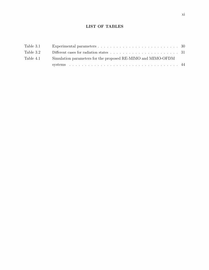
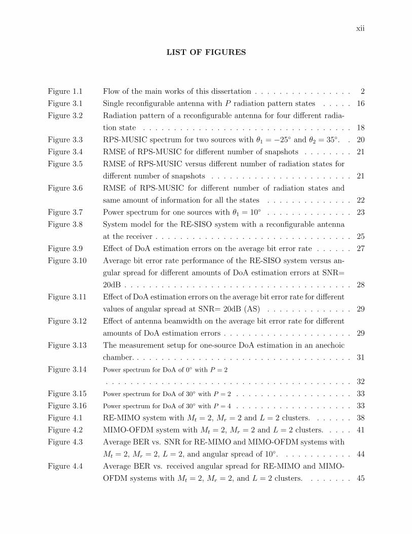
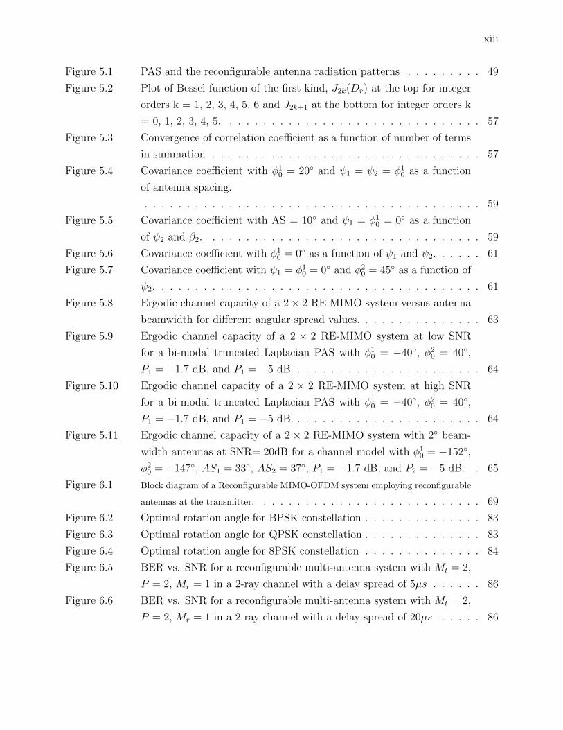
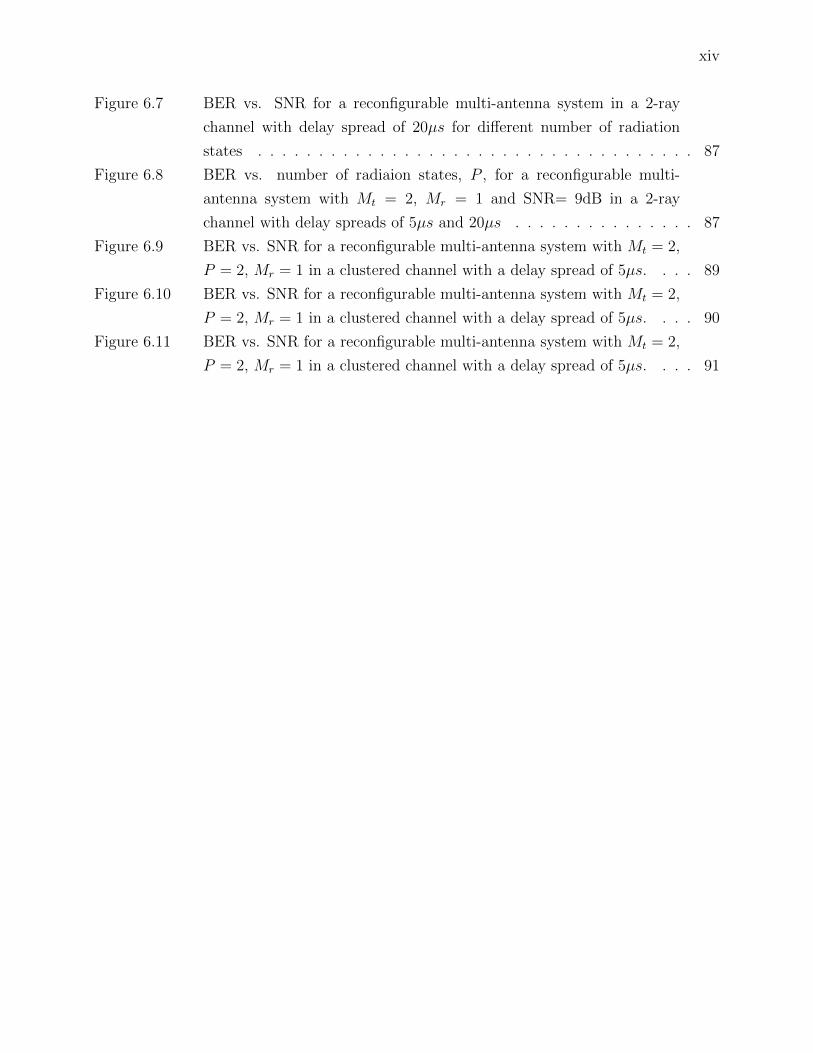
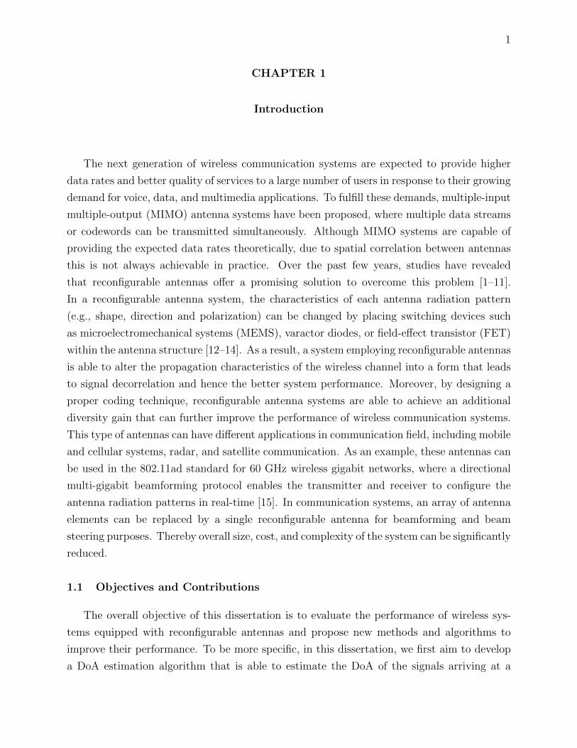
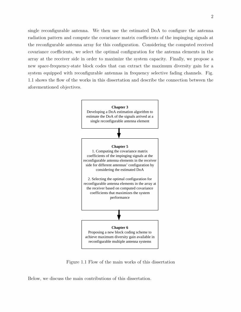
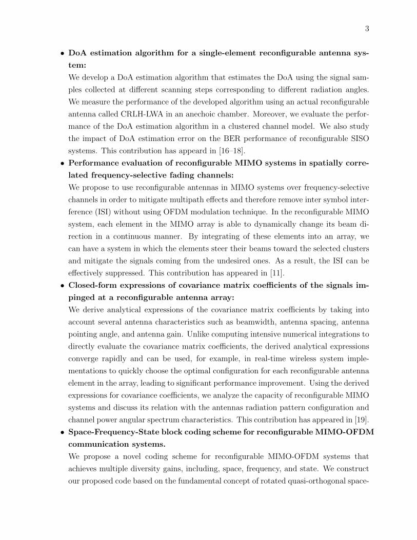
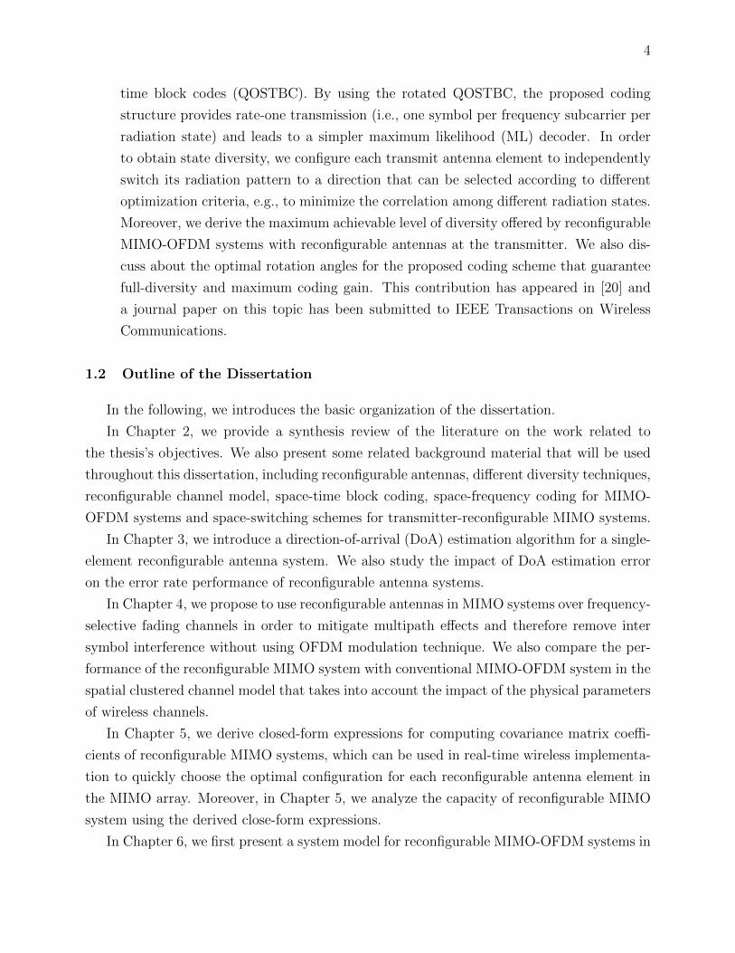
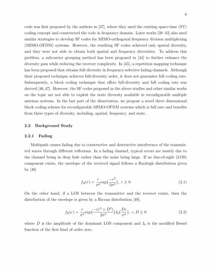
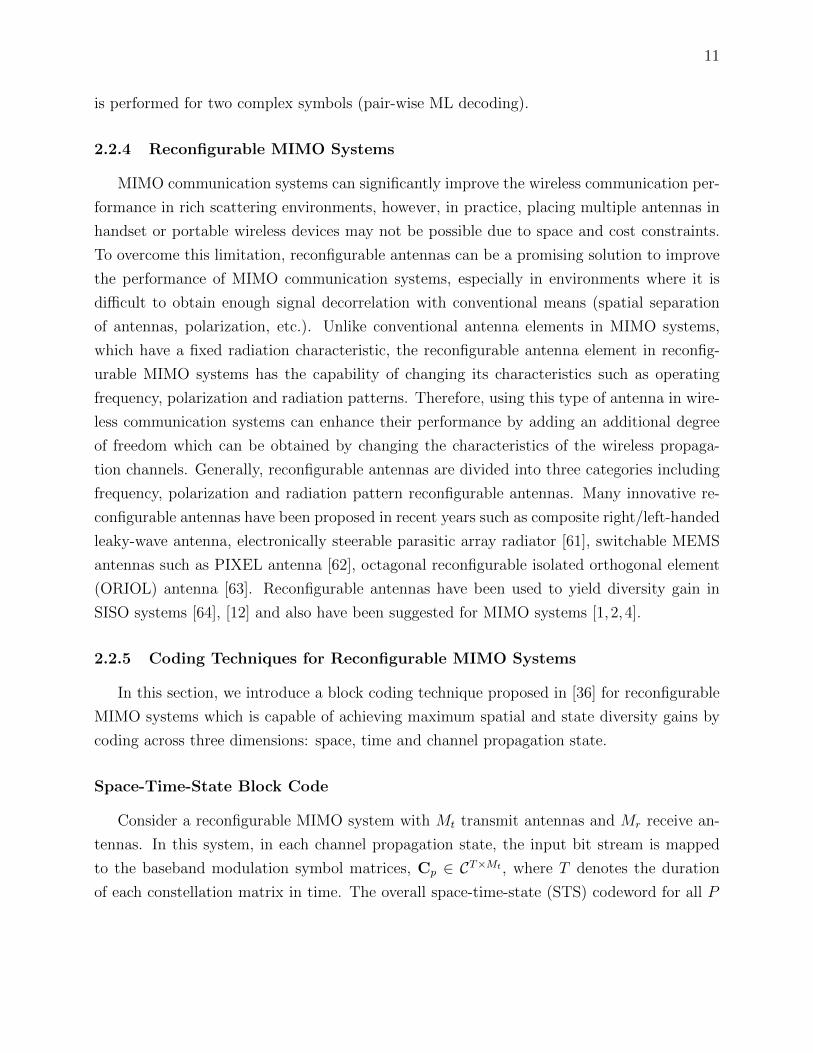
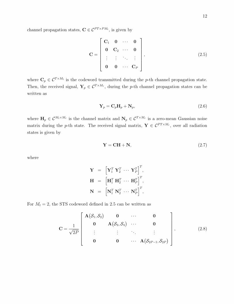
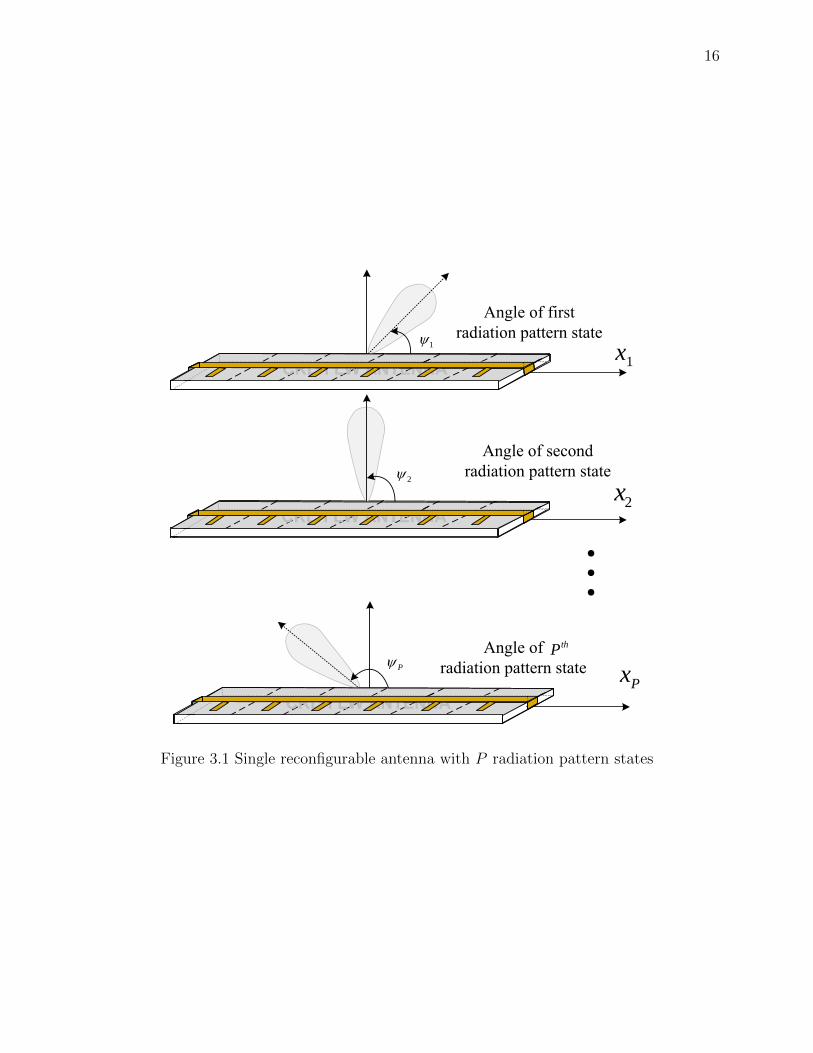
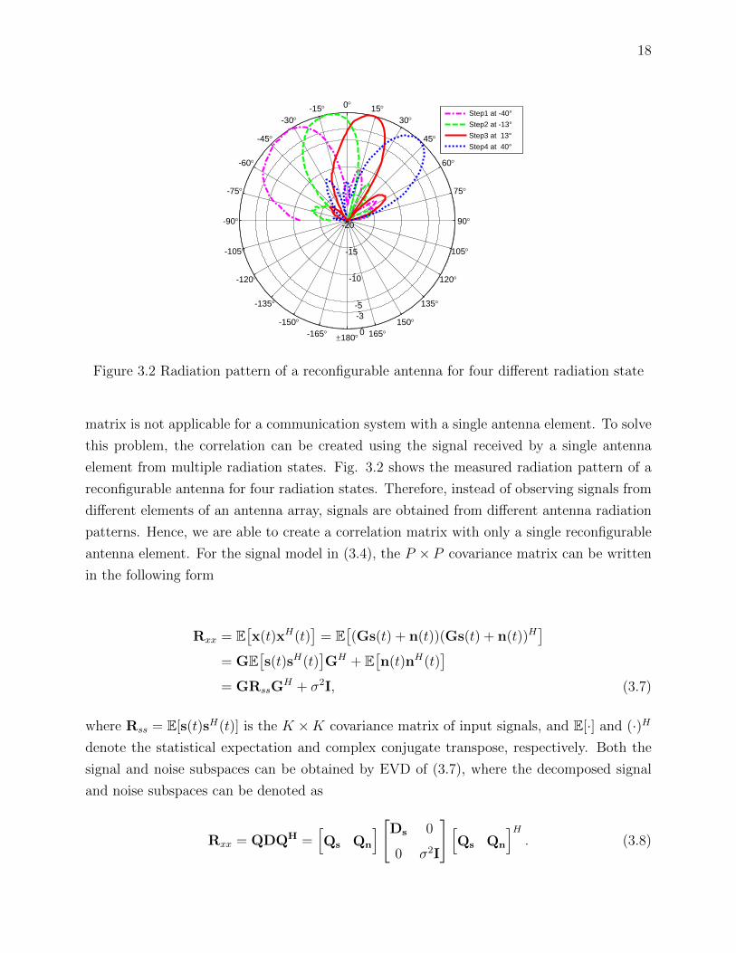
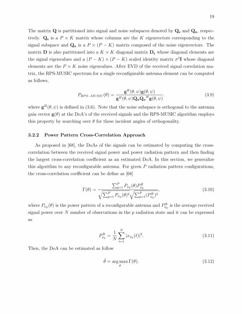
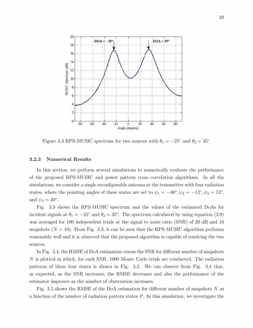
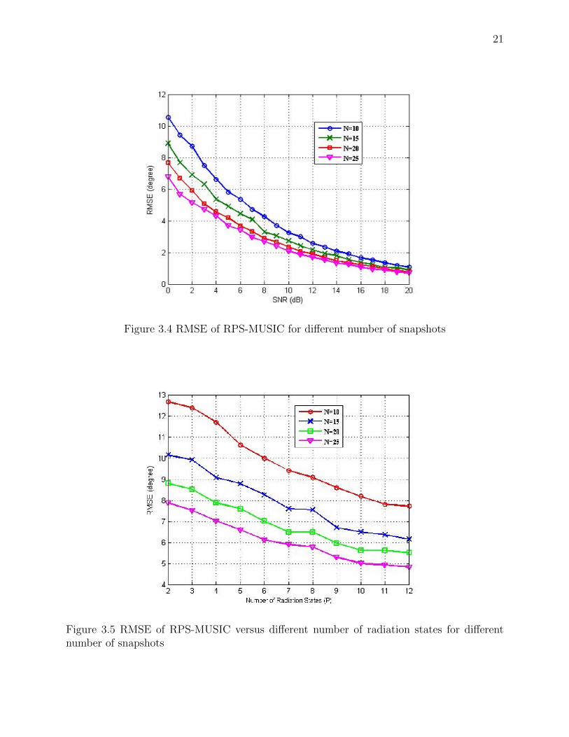
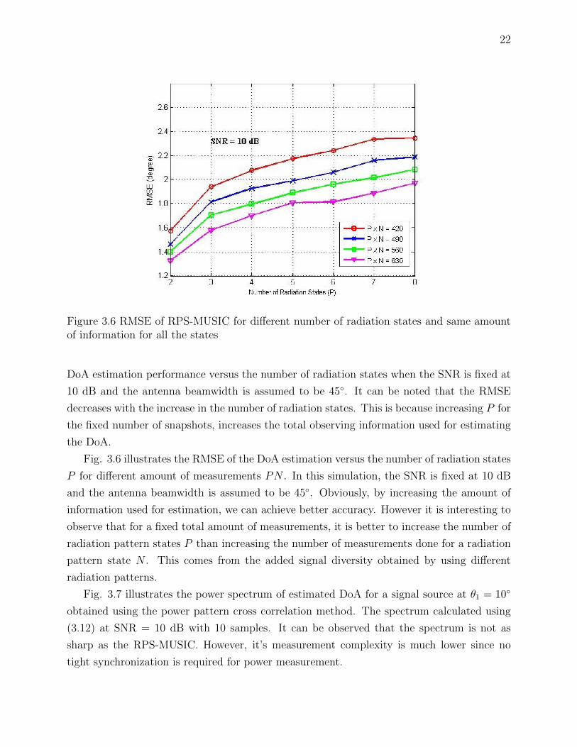
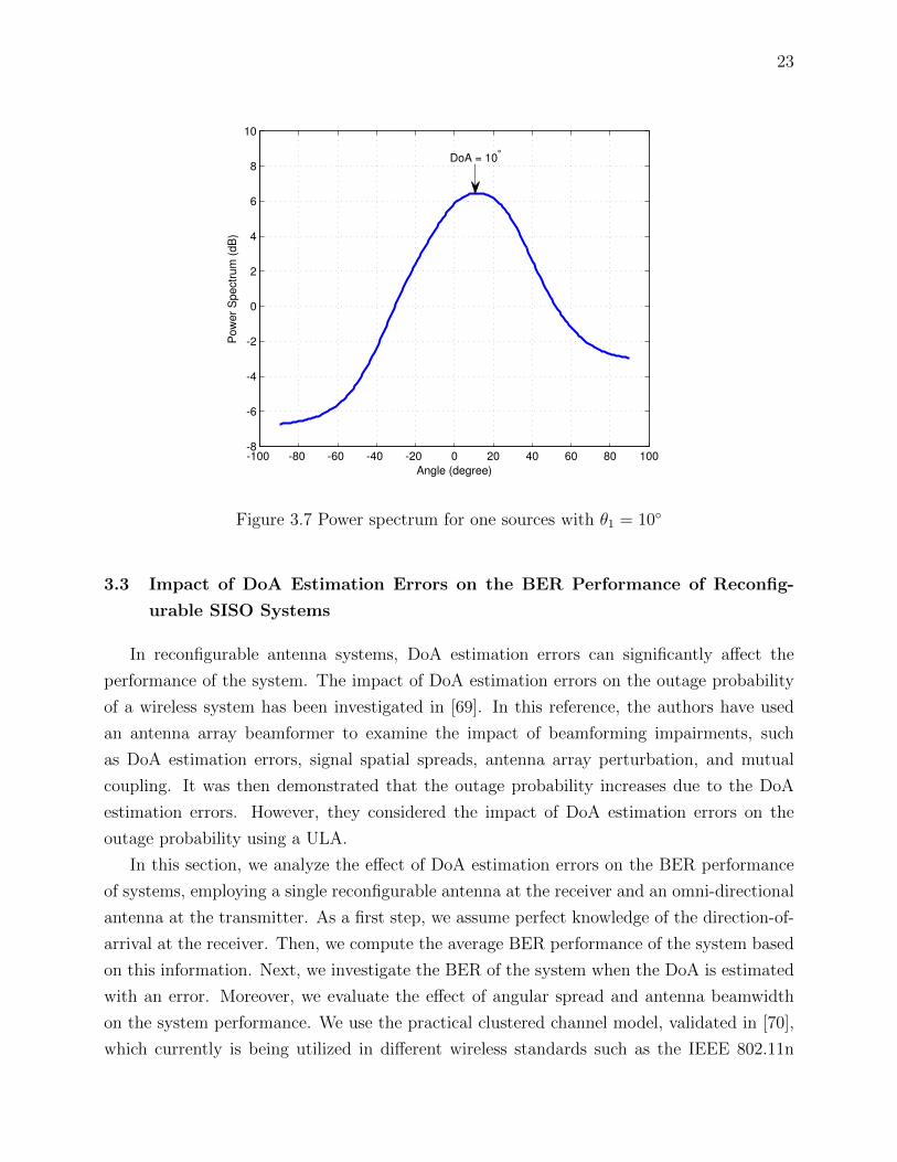
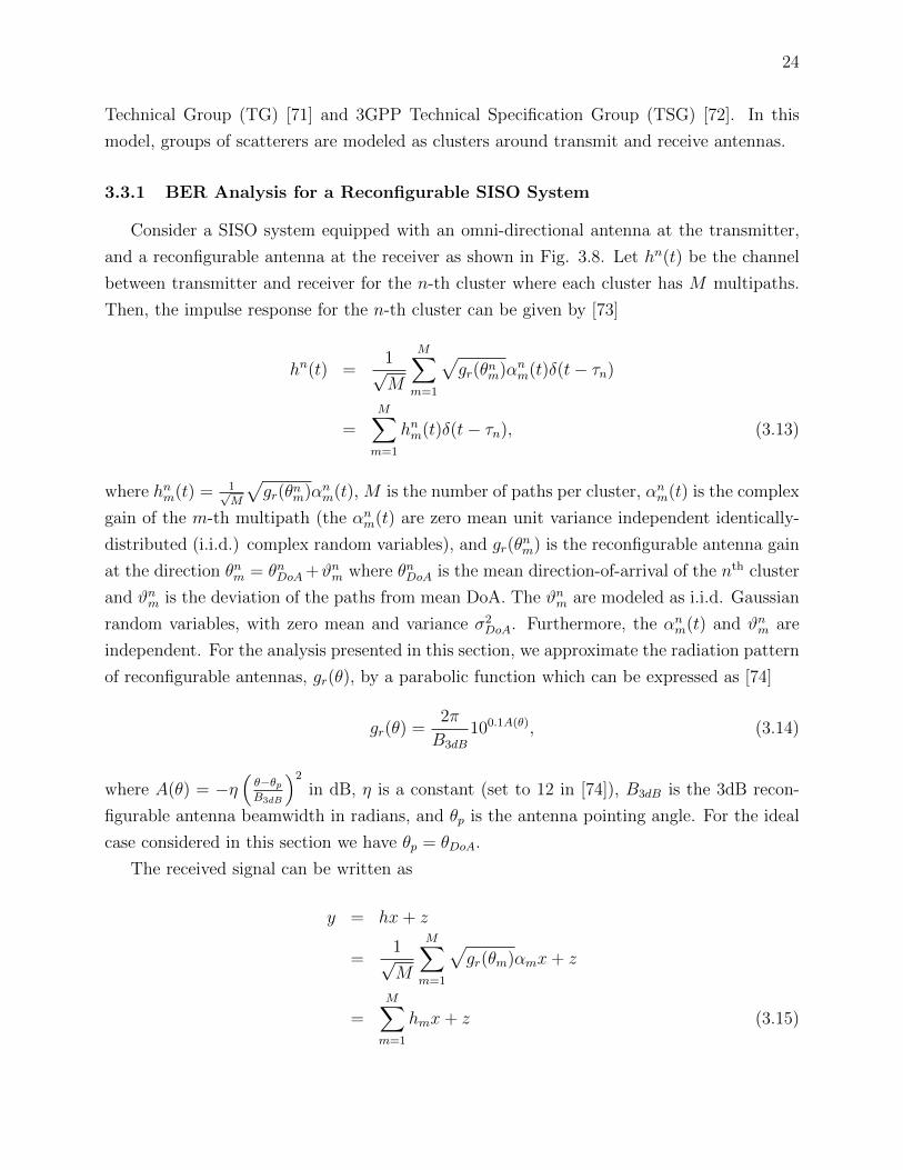
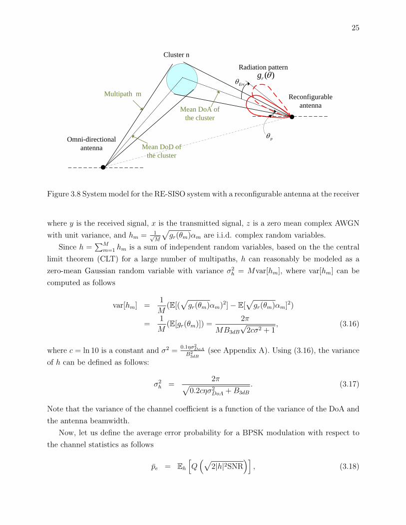
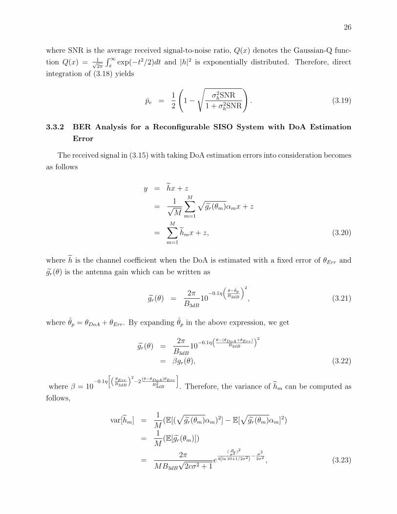
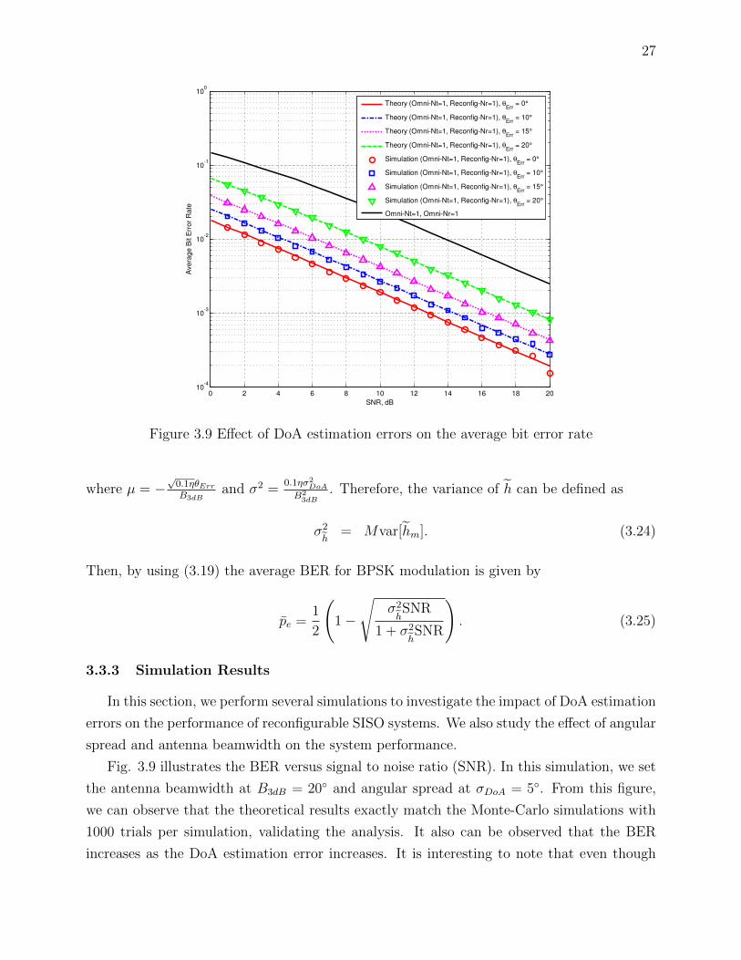
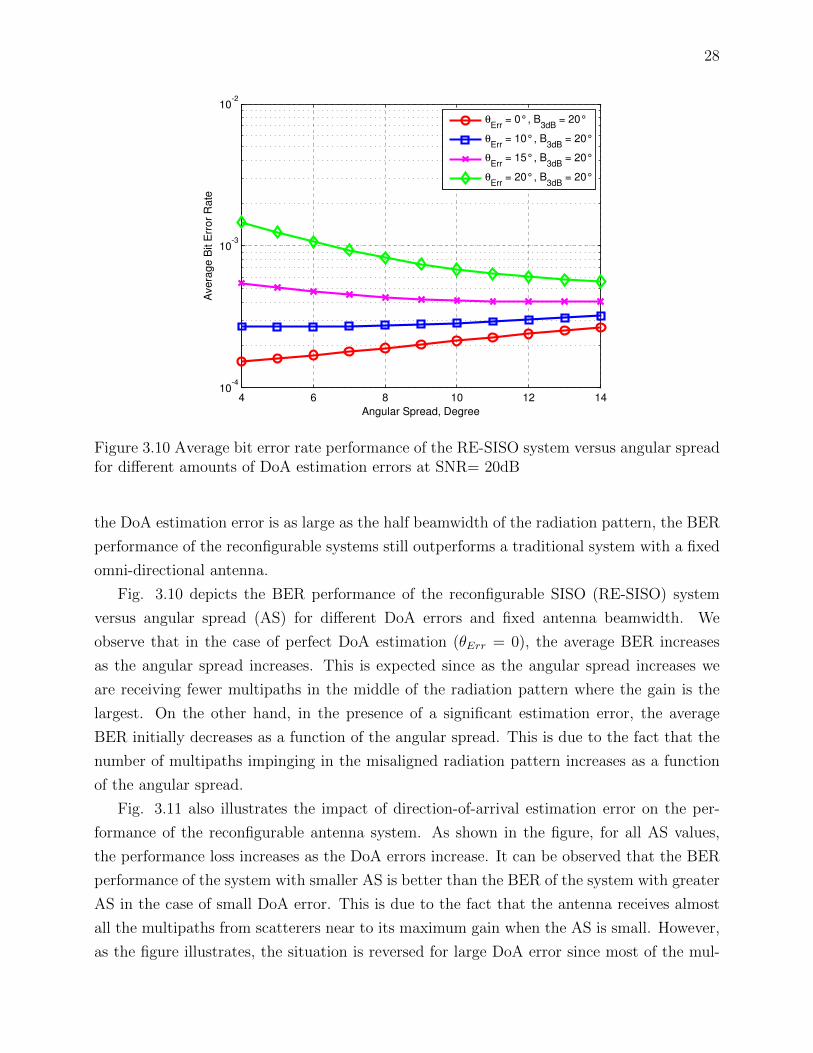
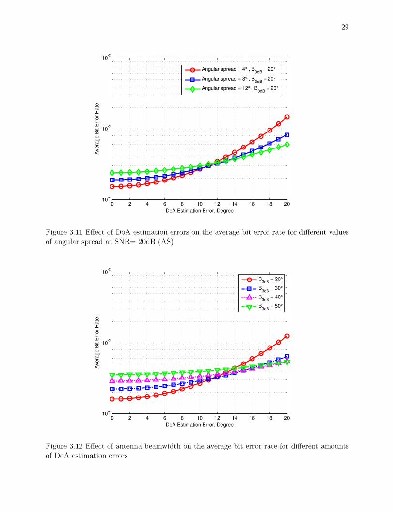
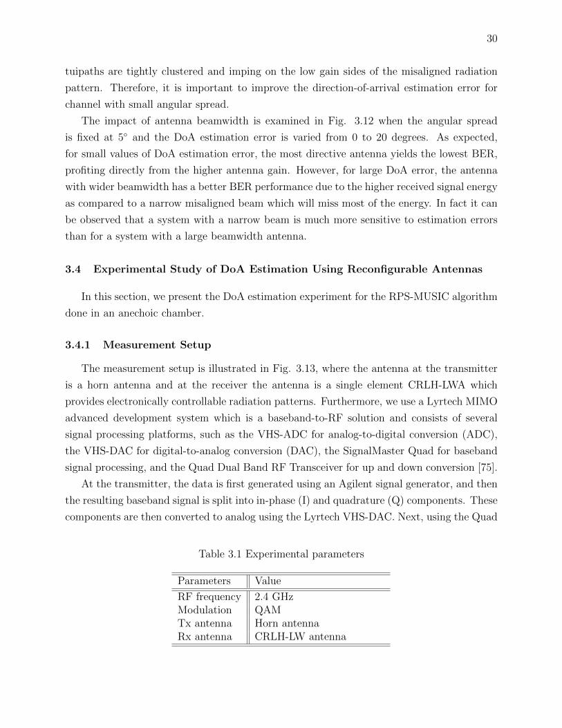
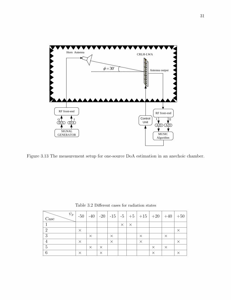
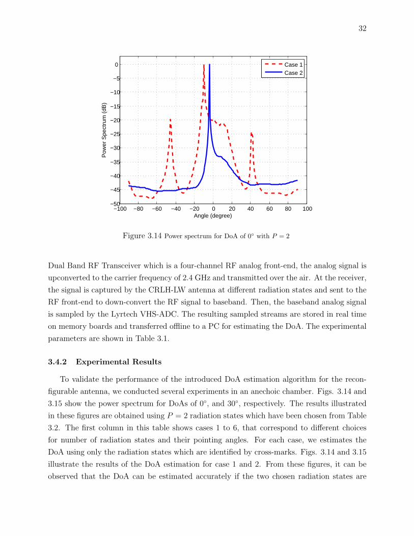
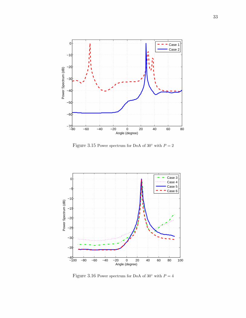
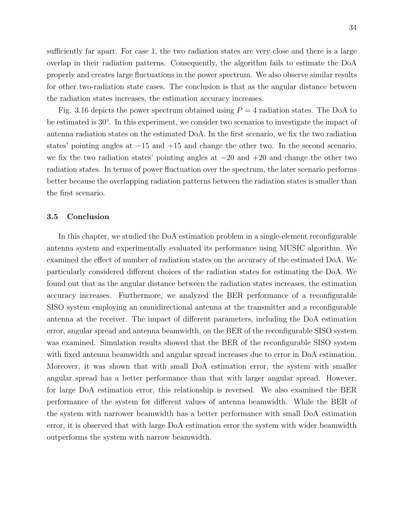
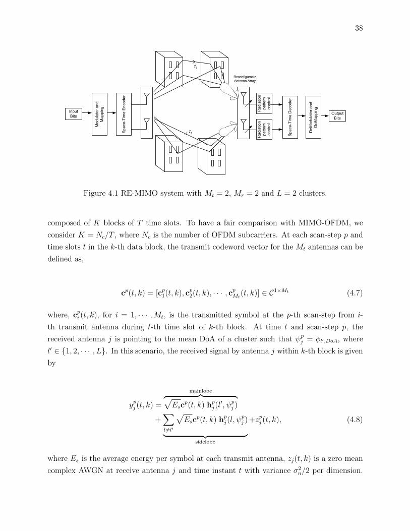
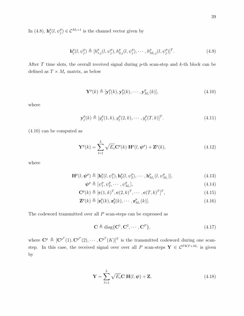
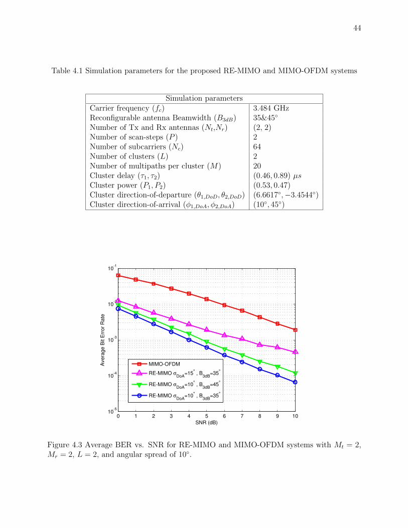
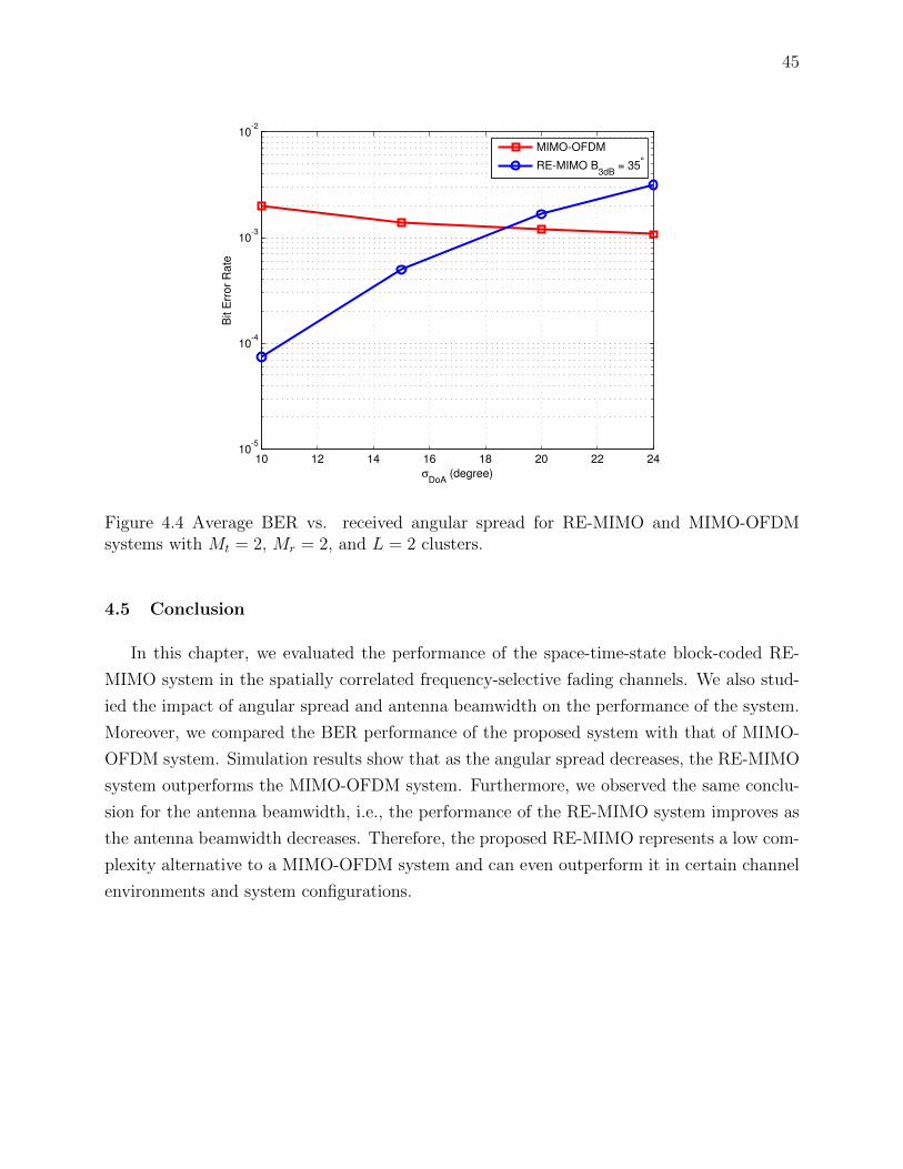
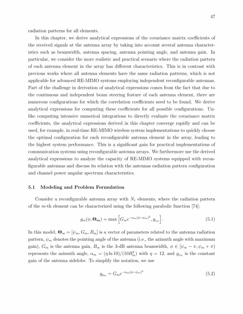
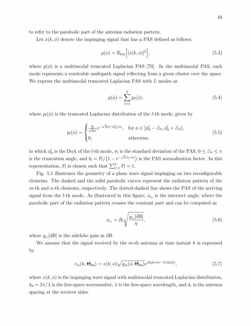
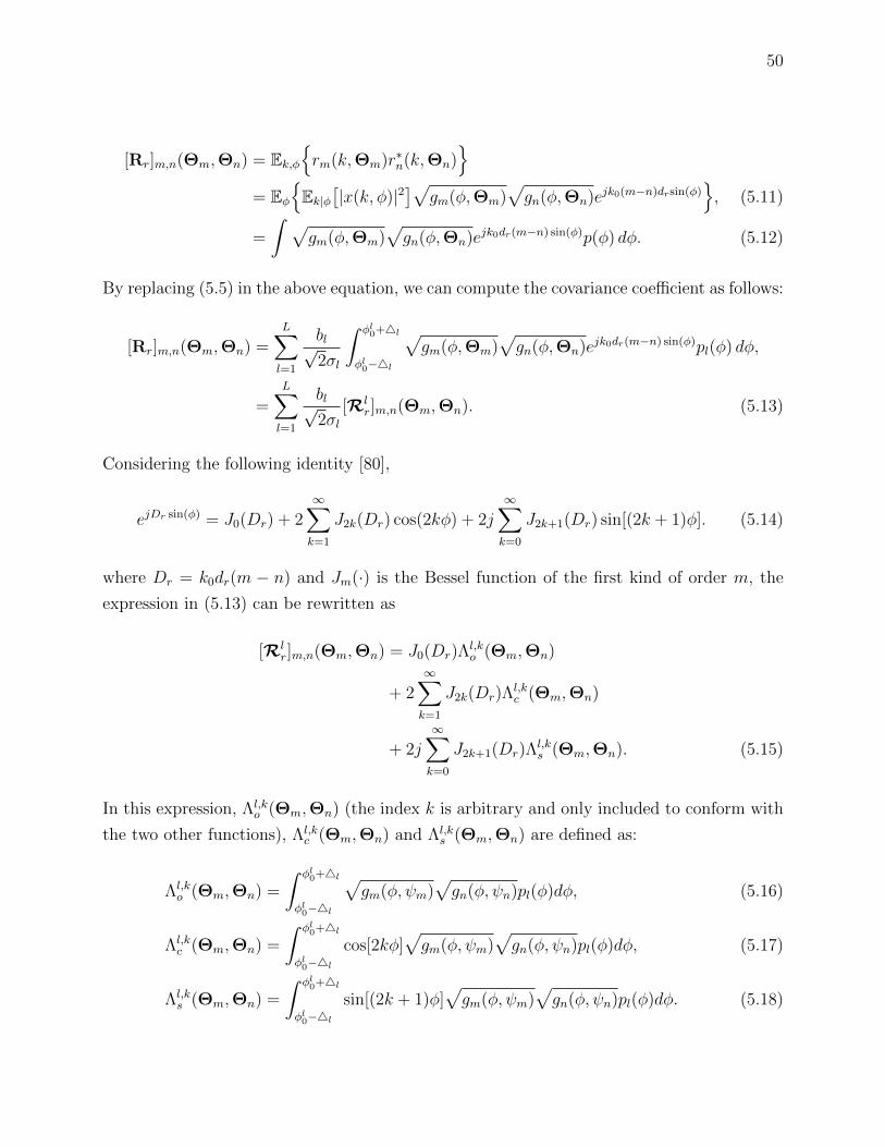
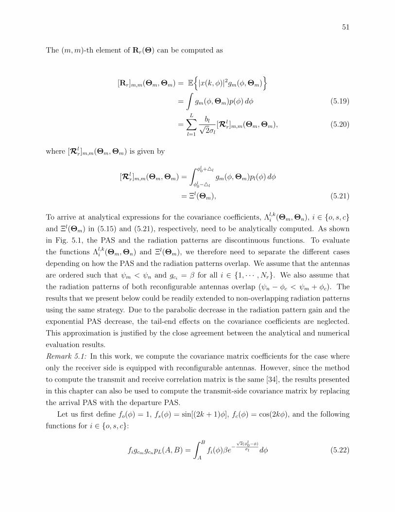
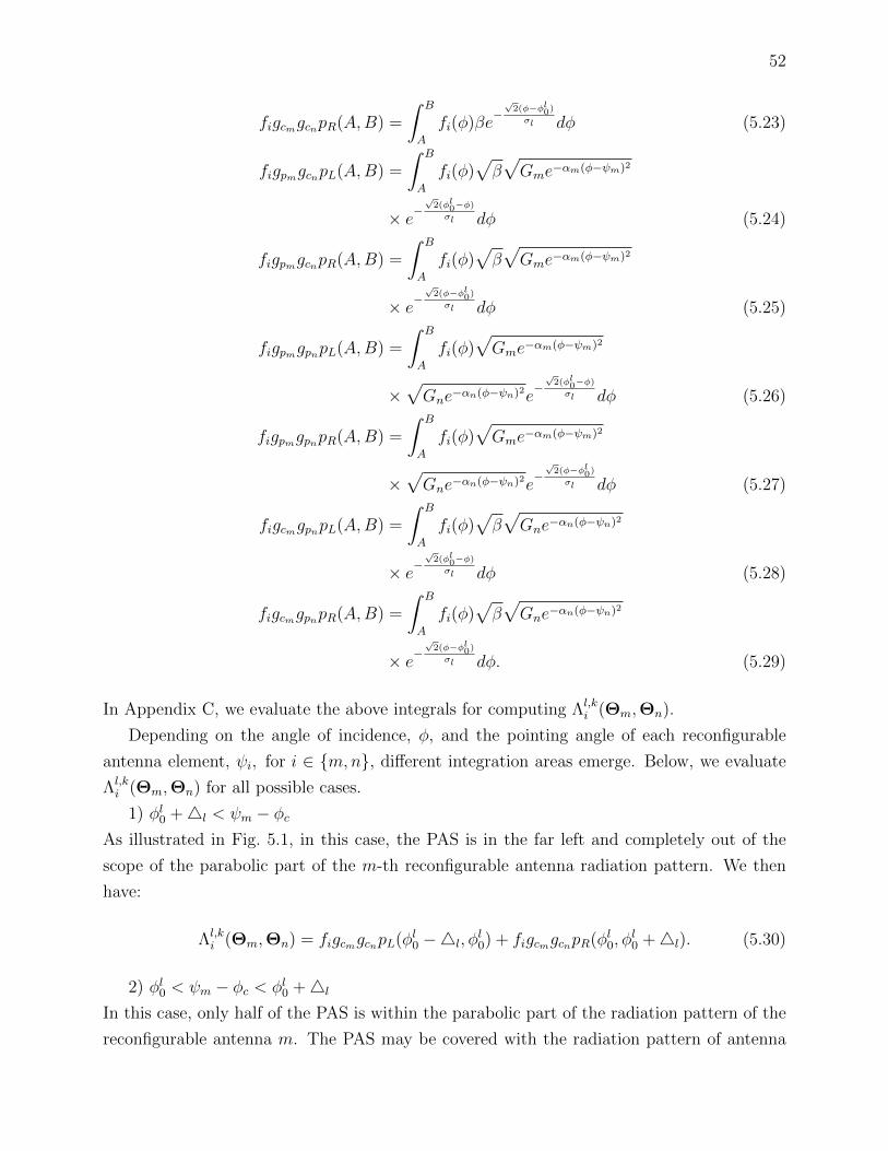
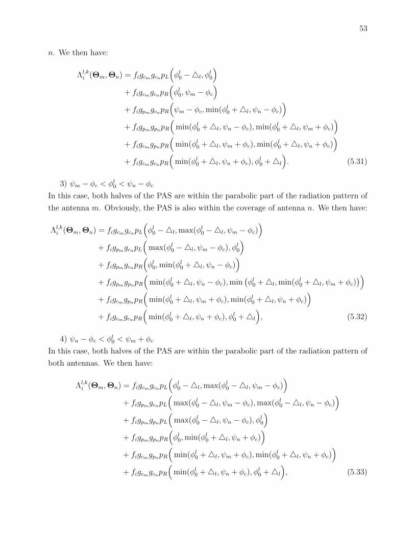
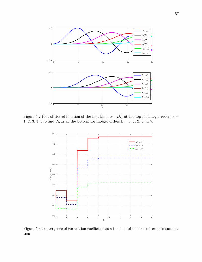
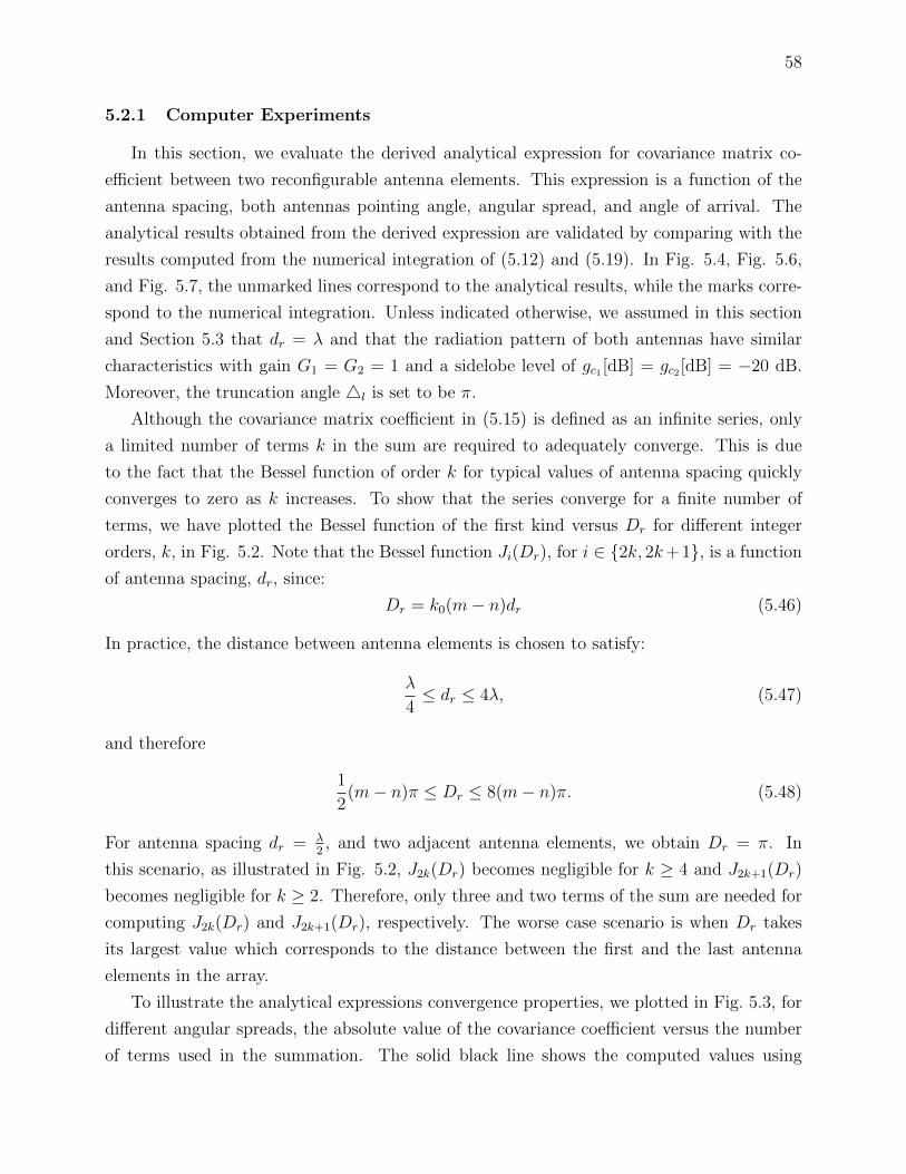
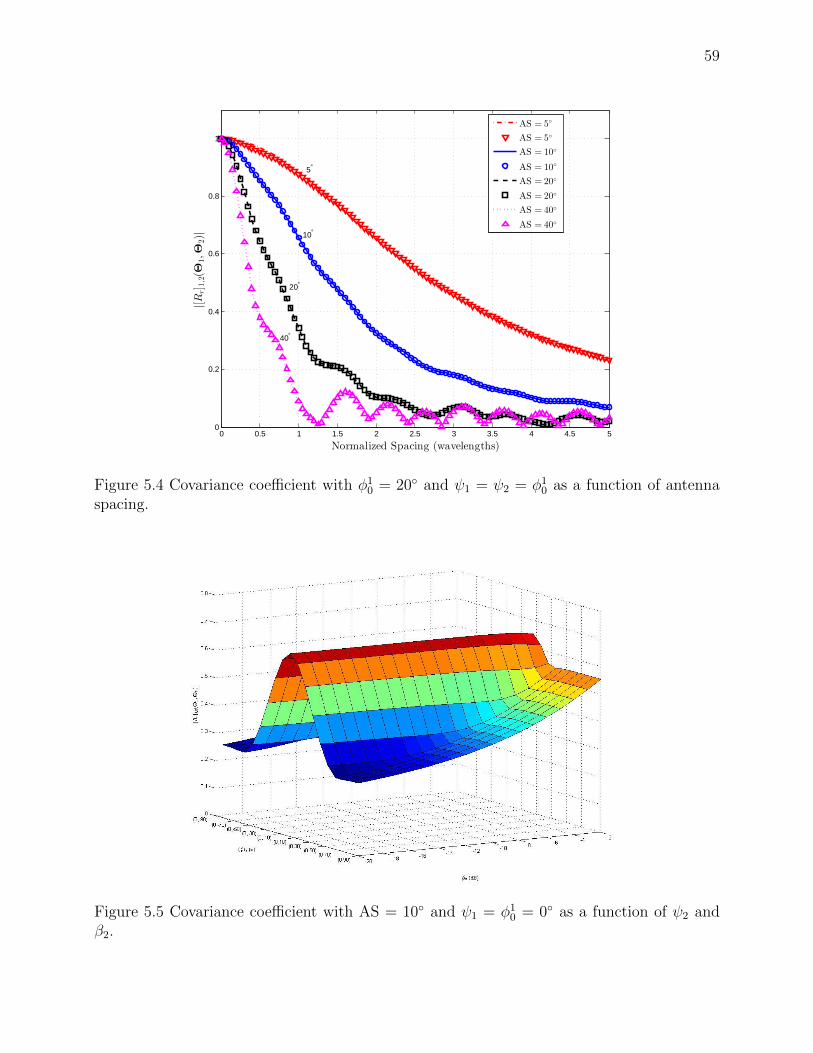
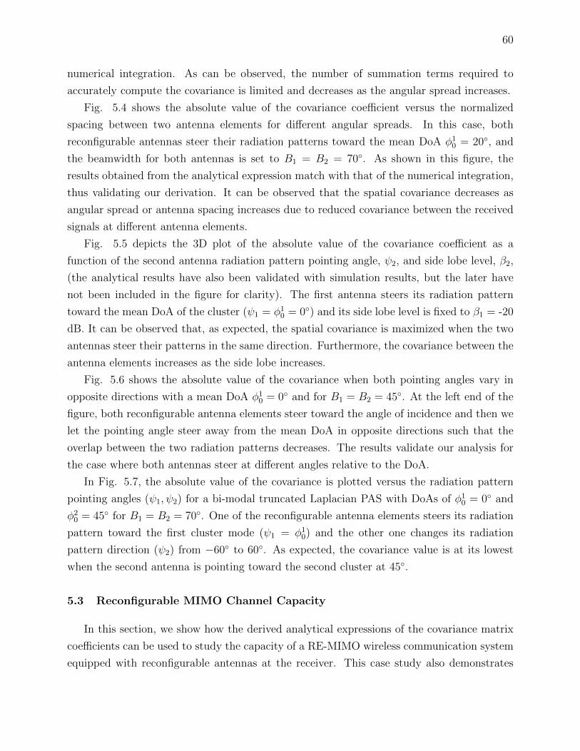
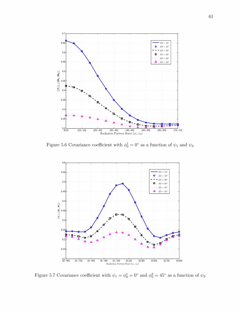
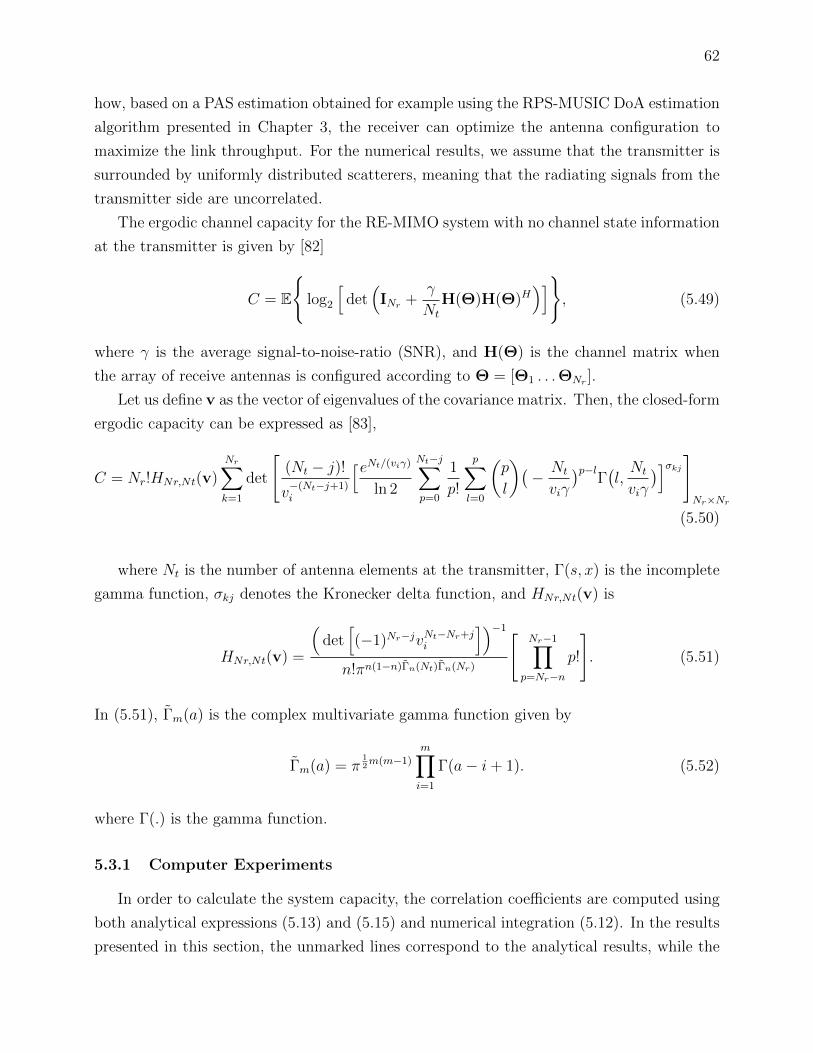
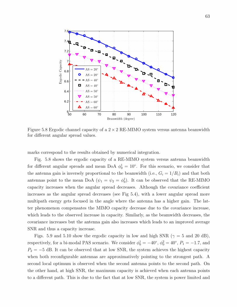
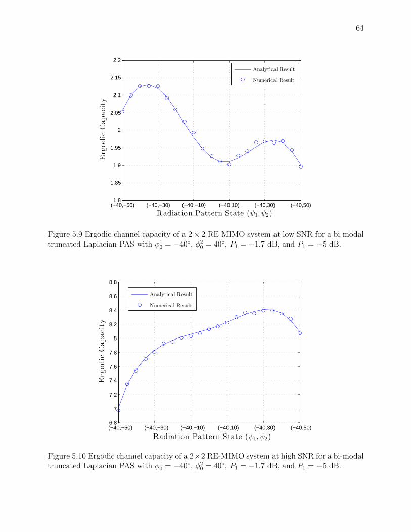
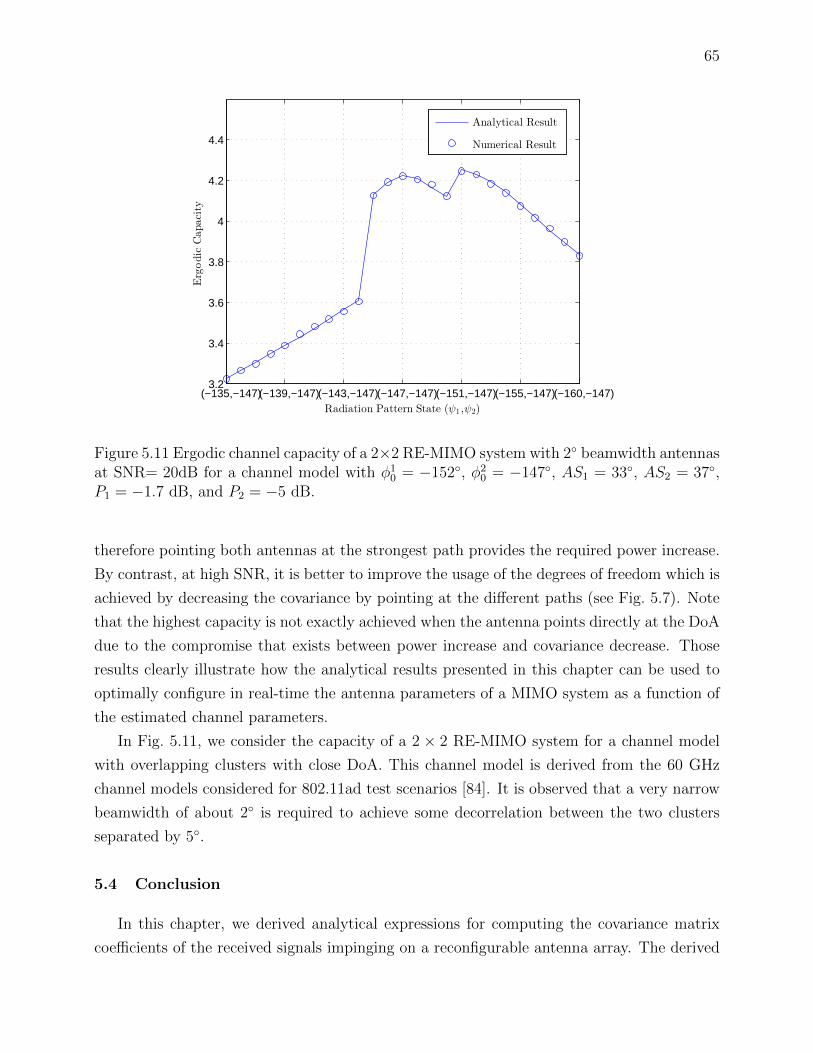
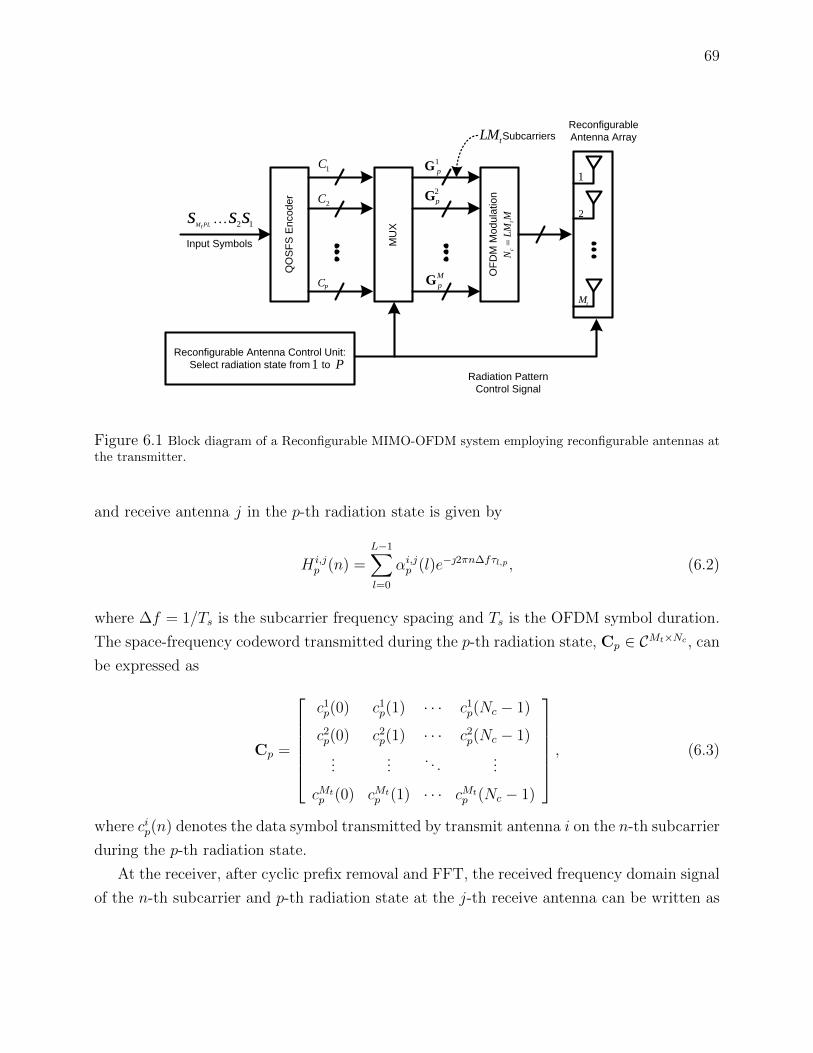
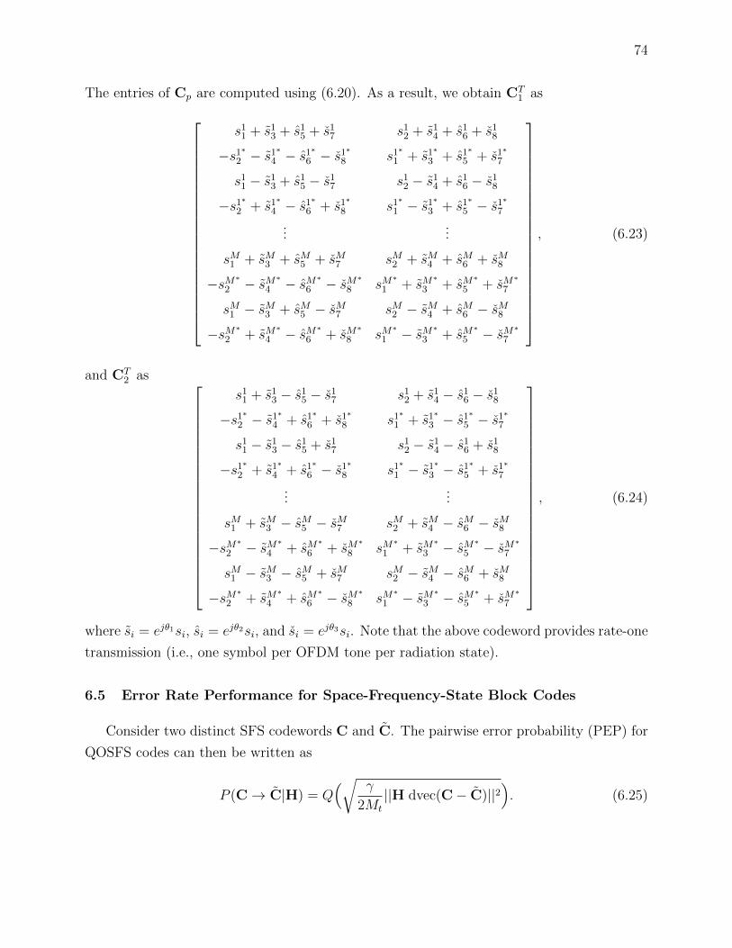
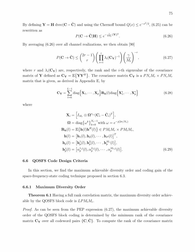
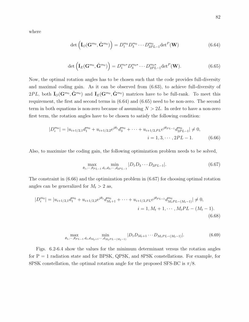
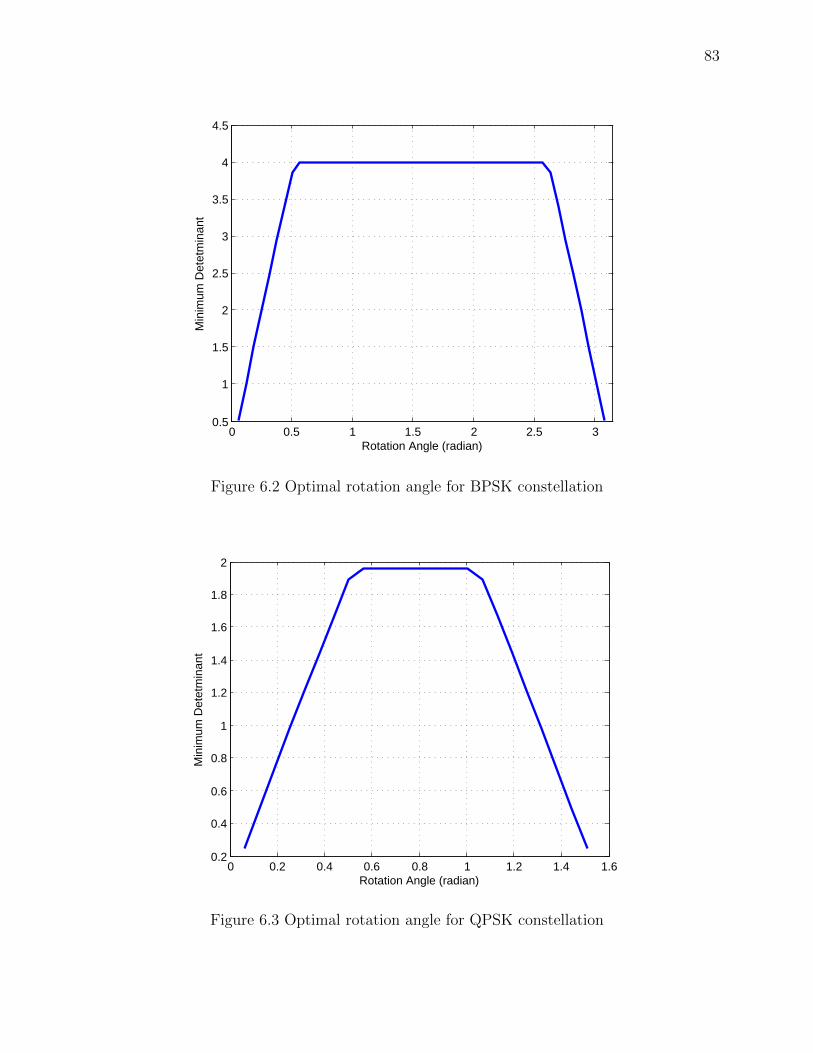
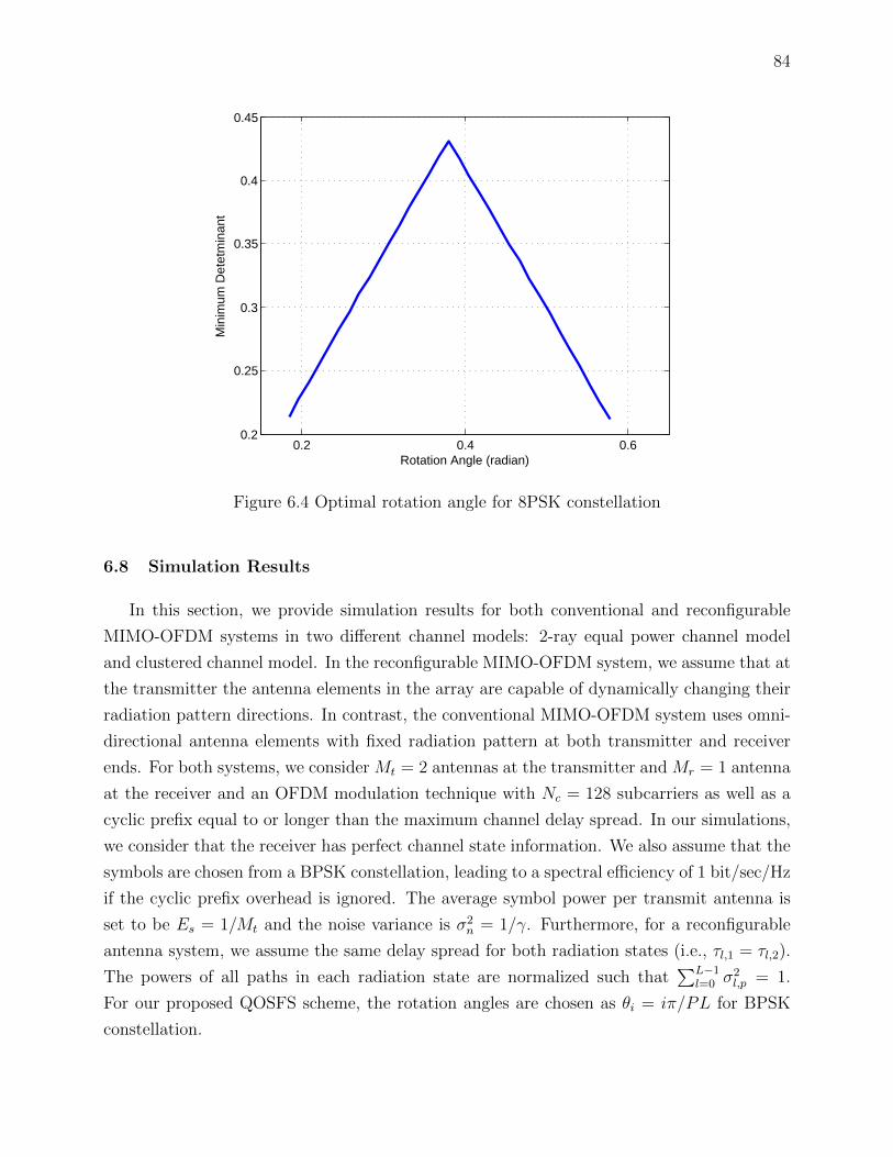
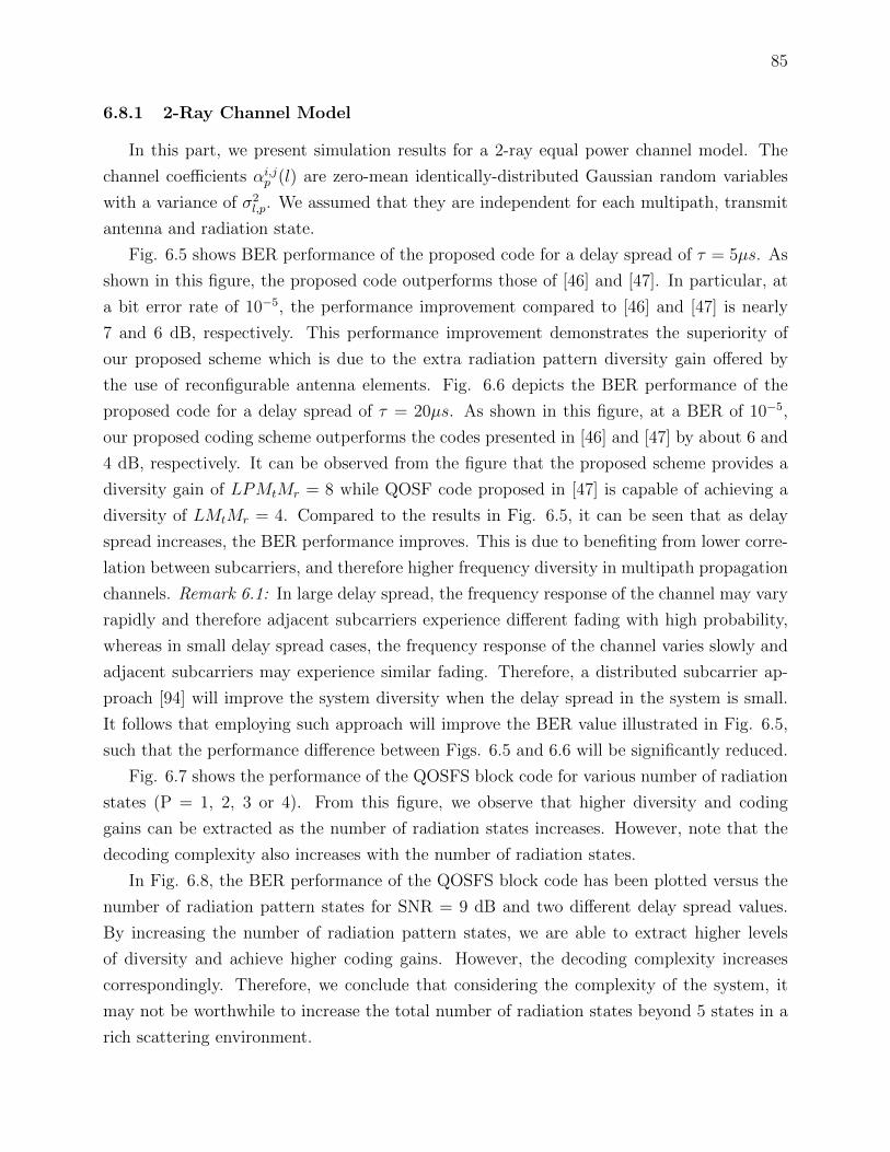
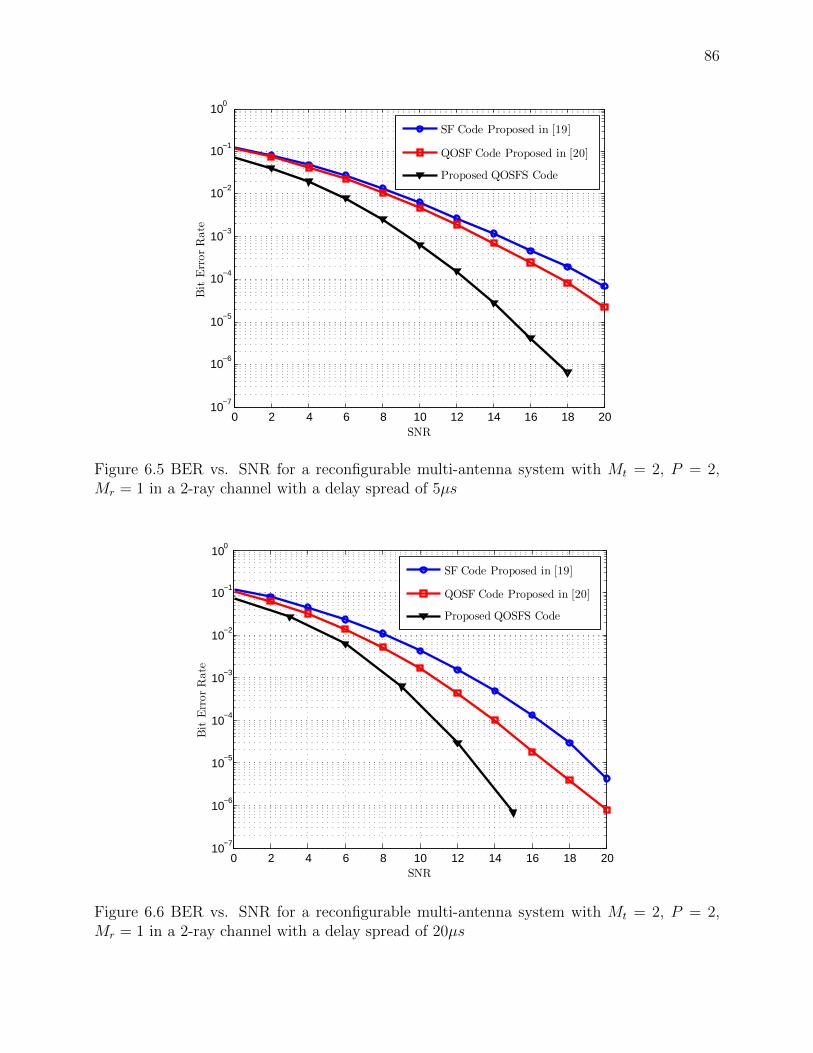
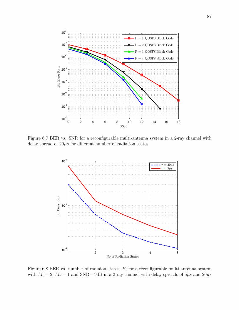
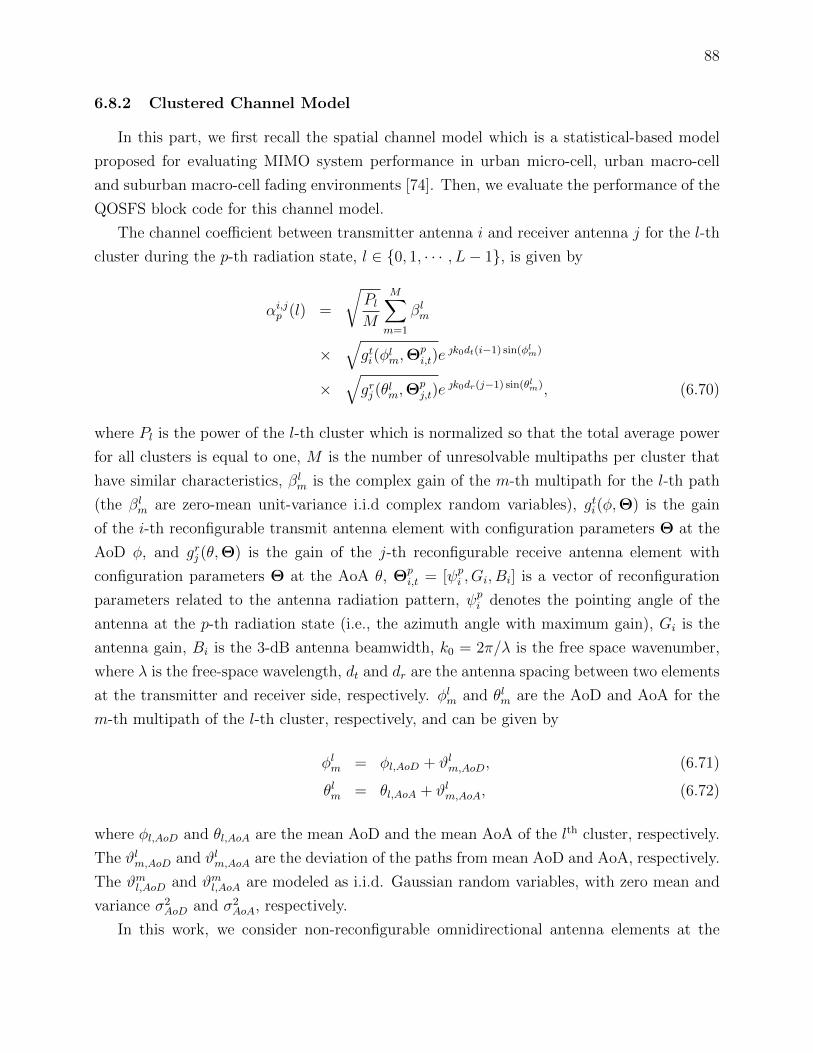
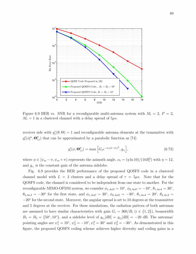
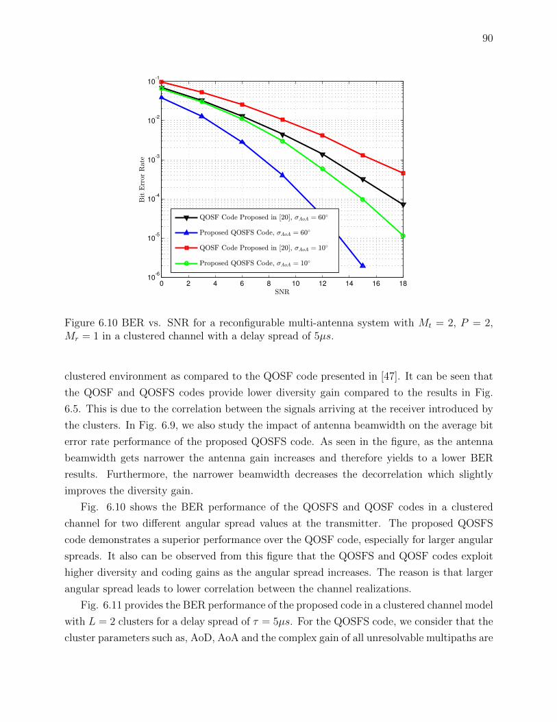
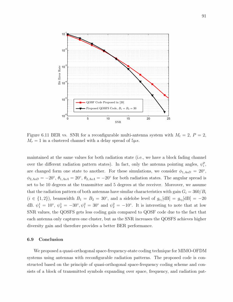
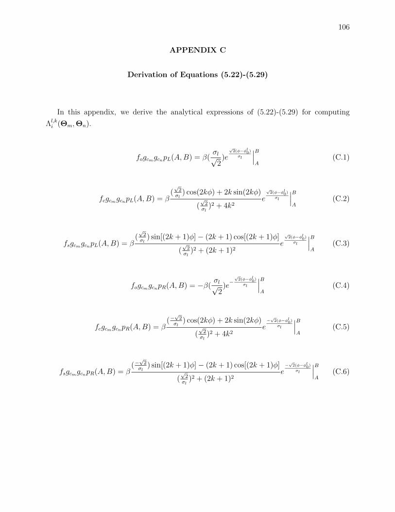
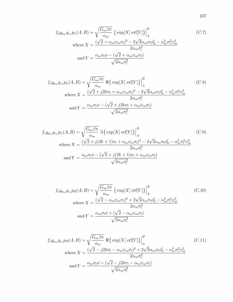
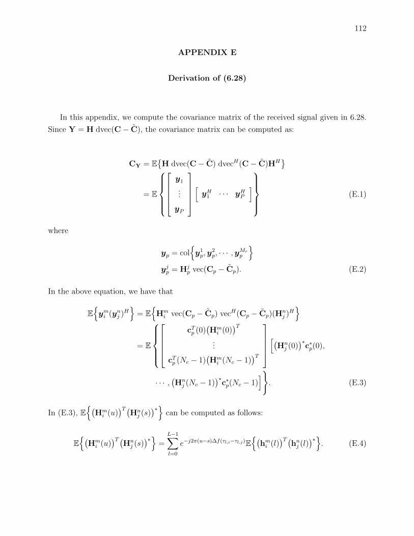
reconfigurable MIMO-OFDM system, we consider φ1,AoD = 10, φ2,AoD = −10, θ1,AoA = 30,
θ2,AoA = −30 for the first state, and φ1,AoD = 30, φ2,AoD = −30, θ1,AoA = 20, θ2,AoA =
−20 for the second state. Moreover, the angular spread is set to 10 degrees at the transmitter
and 5 degrees at the receiver. For these simulations, the radiation pattern of both antennas
are assumed to have similar characteristics with gain Gi = 360/Bi (i ∈ 1, 2), beamwidth
B1 = B2 = 50, 10, and a sidelobe level of gc1 [dB] = gc2 [dB] = −20 dB. The antennas’
pointing angles are ψ11 = 10, ψ1
2 = −10, ψ21 = 30 and ψ2
2 = −30. As demonstrated in this
figure, the proposed QOSFS coding scheme achieves higher diversity and coding gains in a
90
0 2 4 6 8 10 12 14 16 1810
-6
10-5
10-4
10-3
10-2
10-1
SNR
Bit
Err
orR
ate
QOSF Code Proposed in [20], <AoA = 60/
Proposed QOSFS Code, <AoA = 60/
QOSF Code Proposed in [20], <AoA = 10/
Proposed QOSFS Code, <AoA = 10/
Figure 6.10 BER vs. SNR for a reconfigurable multi-antenna system with Mt = 2, P = 2,Mr = 1 in a clustered channel with a delay spread of 5µs.
clustered environment as compared to the QOSF code presented in [47]. It can be seen that
the QOSF and QOSFS codes provide lower diversity gain compared to the results in Fig.
6.5. This is due to the correlation between the signals arriving at the receiver introduced by
the clusters. In Fig. 6.9, we also study the impact of antenna beamwidth on the average bit
error rate performance of the proposed QOSFS code. As seen in the figure, as the antenna
beamwidth gets narrower the antenna gain increases and therefore yields to a lower BER
results. Furthermore, the narrower beamwidth decreases the decorrelation which slightly
improves the diversity gain.
Fig. 6.10 shows the BER performance of the QOSFS and QOSF codes in a clustered
channel for two different angular spread values at the transmitter. The proposed QOSFS
code demonstrates a superior performance over the QOSF code, especially for larger angular
spreads. It also can be observed from this figure that the QOSFS and QOSF codes exploit
higher diversity and coding gains as the angular spread increases. The reason is that larger
angular spread leads to lower correlation between the channel realizations.
Fig. 6.11 provides the BER performance of the proposed code in a clustered channel model
with L = 2 clusters for a delay spread of τ = 5µs. For the QOSFS code, we consider that the
cluster parameters such as, AoD, AoA and the complex gain of all unresolvable multipaths are
91
0 5 10 15 20 2510
-6
10-5
10-4
10-3
10-2
10-1
SNR
Bit
Err
orR
ate
QOSF Code Proposed in [20]
Proposed QOSFS Code, B1 = B2 = 30
Figure 6.11 BER vs. SNR for a reconfigurable multi-antenna system with Mt = 2, P = 2,Mr = 1 in a clustered channel with a delay spread of 5µs.
maintained at the same values for both radiation state (i.e., we have a block fading channel
over the different radiation pattern states). In fact, only the antenna pointing angles, ψpi ,
are changed form one state to another. For these simulations, we consider φ1,AoD = 20,
φ2,AoD = −20, θ1,AoA = 20, θ2,AoA = −20 for both radiation states. The angular spread is
set to be 10 degrees at the transmitter and 5 degrees at the receiver. Moreover, we assume
that the radiation pattern of both antennas have similar characteristics with gainGi = 360/Bi
(i ∈ 1, 2), beamwidth B1 = B2 = 30, and a sidelobe level of gc1 [dB] = gc2 [dB] = −20
dB. ψ11 = 10, ψ1
2 = −30, ψ21 = 30 and ψ2
2 = −10. It is interesting to note that at low
SNR values, the QOSFS gets less coding gain compared to QOSF code due to the fact that
each antenna only captures one cluster, but as the SNR increases the QOSFS achieves higher
diversity gain and therefore provides a better BER performance.
6.9 Conclusion
We proposed a quasi-orthogonal space-frequency-state coding technique for MIMO-OFDM
systems using antennas with reconfigurable radiation patterns. The proposed code is con-
structed based on the principle of quasi-orthogonal space-frequency coding scheme and con-
sists of a block of transmitted symbols expanding over space, frequency, and radiation pat-
92
tern state dimensions. We evaluated the diversity and coding gains of the proposed code,
and provide the criteria to select the code rotation angles to optimize the code performance
and achieve maximum diversity. We provided simulation results to demonstrate the perfor-
mance of the proposed coding scheme and make comparisons with that of previous SF coding
schemes. In these experiments, it has been shown that the proposed code provides additional
diversity and coding gains compared to the previously designed SF codes in MIMO-OFDM
systems.
93
CHAPTER 7
Conclusion
We here summarize the work in this dissertation and discuss some of the foreseeable future
research directions that this research may lead to.
7.1 Summary
In this dissertation, we first introduced a DoA estimation algorithm for a single-element
reconfigurable antenna system. We then evaluated the performance of this algorithm in an
anechoic chamber using an actual reconfigurable antenna called CRLH-LWA. We examined
the effect of number of scanning steps on the accuracy of the estimated DoA. From the
results, we observed that the DoA can be estimated accurately if the two chosen scanning
steps are sufficiently far apart. In the case of having two scanning steps where they are
very close and there is a large overlap in their radiation patterns, the algorithm fails to
estimate the DoA properly and creates large fluctuations in the power spectrum. Moreover,
we examined the impact of the DoA estimation error on the BER of the reconfigurable SISO
system. Simulation results showed that the BER of the RE-SISO system with fixed antenna
beamwidth and angular spread increases due to error in DoA estimation. Furthermore, it
was shown that with small DoA estimation error, the system with smaller angular spread
has a better performance than that with larger angular spread. However, for large DoA
estimation error, this relationship is reversed. We also examined the BER performance of
the system for different values of antenna beamwidth. While the BER of the system with
narrower beamwidth has a better performance in small DoA estimation error, it is observed
that in large DoA estimation error the system with wider beamwidth outperforms the system
with narrower bandwidth.
In the following part of the dissertation, we proposed a low-complexity MIMO system
employing reconfigurable antennas with electronically controllable radiation patterns over
the frequency-selective channels to mitigate multipath effects and therefore remove inter
symbol interference without using OFDM modulation technique. We studied the impact of
angular spread and antenna beamwidth on its performance and make comparison with that
of MIMO-OFDM system. We observed that as the angular spread decreases, the proposed
RE-MIMO outperforms the MIMO-OFDM system. We also showed that the performance of
the RE-MIMO system improves as the antenna beamwidth decreases.
94
In the next part of this dissertation, we derived analytical expressions for computing
covariance matrix coefficients of the received signals impinging on a reconfigurable antenna
array. The derived expressions were validated using a numerical integration method. We
investigated the impact of radiation pattern characteristics and array configurations on the
covariance coefficients. We also studied the capacity of a reconfigurable MIMO system using
the derived analytical expressions. We showed how the presented results can be used to
quickly choose the optimal configuration for each reconfigurable antenna element in the array.
In the last part of this dissertation, we proposed a space-frequency coding technique for
MIMO-OFDM systems using antennas with reconfigurable radiation patterns. The proposed
code is constructed based on the principle of quasi-orthogonal coding scheme and consists
of a block of transmitted symbols expanding over space, frequency, and radiation state di-
mensions. We provided simulation results to demonstrate the performance of the proposed
coding scheme and make comparisons with that of the previous SF coding schemes. In these
experiments, it has been shown that the proposed code provides additional diversity and
coding gains compared to the previously designed SF codes in MIMO-OFDM systems.
The developed algorithms and schemes in this dissertation can be used in 5th genera-
tion (5G) of wireless communication systems. As an example, our proposed block coding
technique in Chapter 6 can be deployed in millimeter-wave wireless gigabit networks, where
directional beamforming with real-time radiation pattern configuration and OFDM modula-
tion are considered as key technologies to improve the BER performance of the system in an
open-loop mode. The analytical expressions derived in Chapter 5 can be adopted in 5G to
find the optimal radiation configuration at the receiver to enhance the system capacity. The
correlation coefficients information obtained using the derived expressions can also be shared
with the transmitter in a closed-loop system to find a superior transmission state, which can
be utilized for the proposed space-frequency-state block code in Chapter 6.
In summary, in this dissertation, we achieve our stated general objectives by evaluating the
performance of reconfigurable antenna systems and proposing new methods and algorithms
to improve the system performance.
7.2 Future Works
A number of possible extensions of the research presented in this dissertation are briefly
described below:
– In this dissertation, we derived the closed-form expressions for computing covariance
matrix coefficients of the received signals at a reconfigurable antenna array. Using these
expressions, we studied the capacity of a reconfigurable MIMO system for different ra-
95
diation pattern states. The future research direction in this area can be defined as to
develop an optimal selection algorithm to choose the optimal configuration for each
reconfigurable antenna element in the array that maximizes the system capacity based
on the computed correlation coefficients using derived close-form expressions.
– Throughout this dissertation, we considered in the theoretical analysis a parabolic func-
tion model for the radiation pattern of a reconfigurable antenna. In this model, the
antenna only steers in azimuth plane. Another extension of this work is to include
vertical cuts as well which is needed for millimeter wave communications standard as
beam steering will be required for both vertical and horizontal cuts. In this respect, the
channel model also needs to be extended to include elevation power angular spectrum.
In cases where a two-dimensional Laplacian or a general double exponential functions
can model the incoming signal distribution, a similar methodology as the one presented
in this dissertation can then be followed to obtain series expressions for the covariance
matrix coefficients. However, the number of cases to be considered will increase as there
is an extra variable to consider.
– In this dissertation, we focused on designing three dimensional block codes. One ex-
tension of this work is to consider the generalization of three dimensional block codes
to n dimensional block codes where n is greater than three. Assume n = 4 which adds
another orthogonal resource to the three dimensional channel model introduced in this
dissertation. A simple method of designing four dimensional block codes based on the
three dimensional block codes presented in this dissertation, is to apply a repetition
coding over the forth orthogonal dimension.
– Throughout this dissertation, we have incorporated coherent detection schemes which
require the knowledge of channel information at the receiver. However, due to the
presence of multiple propagation at both the transmitter and the receiver, the channel
estimation problem is more complicated and costly compared to a non-reconfigurable
MIMO system. Novel channel estimation methods and techniques are required to make
efficient channel estimation for reconfigurable MIMO systems possible.
96
Bibliography
[1] B. Cetiner, H. Jafarkhani, J. Qian, H. Yoo, A. Grau, and F. De Flaviis, “Multifunc-
tional reconfigurable MEMS integrated antennas for adaptive MIMO systems,” IEEE
Communications Magazine, vol. 42, pp. 62–70, Dec. 2004.
[2] B. Cetiner, J. Qian, G. Li, and F. De Flaviis, “A reconfigurable spiral antenna for adap-
tive MIMO systems,” EURASIP Journal on Wireless Communications and Networking,
vol. 2005, pp. 382–389, Mar. 2005.
[3] T. Roach, G. Huff, and J. Bernhard, “On the applications for a radiation reconfigurable
antenna,” in Proc. Second NASA/ESA Conference on Adaptive Hardware and Systems,
AHS, Edinburgh, UK, Aug. 2007, pp. 7–13.
[4] B. Cetiner, E. Akay, E. Sengul, and E. Ayanoglu, “A MIMO system with multifunctional
reconfigurable antennas,” IEEE Antennas and Wireless Propagation Letters, vol. 5, pp.
463–466, Jan. 2006.
[5] D. Piazza, N. Kirsch, A. Forenza, R. Heath, and K. Dandekar, “Design and evalua-
tion of a reconfigurable antenna array for MIMO systems,” IEEE Trans. Antennas and
Propagat., vol. 56, pp. 869–881, Mar. 2008.
[6] A. Grau, H. Jafarkhani, and F. De Flaviis, “A reconfigurable multiple-input multiple-
output communication system,” IEEE Trans. Wireless Commun., vol. 7, pp. 1719–1733,
May 2008.
[7] J. Frigon, C. Caloz, and Y. Zhao, “Dynamic radiation pattern diversity (DRPD) MIMO
using CRLH leaky-wave antennas,” in Proc. IEEE Radio and Wireless Symposium, Jan.
2008, pp. 635–638.
[8] A. Yokoi, T. Mitsui, B.-T. Yoon, and Y.-E. Kim, “Improvement of channel capacity on
MIMO antenna systems with antenna pattern selection,” in Proc. IEEE Int. Symp. on
Antennas and Propagat., Honolulu, HI, Jun. 2007, pp. 3249–3252.
[9] J. D. Boerman and J. T. Bernhard, “Performance study of pattern reconfigurable anten-
nas in MIMO communication systems,” IEEE Trans. Antennas and Propagat., vol. 56,
pp. 231–236, Jan. 2008.
[10] H. Eslami, C. P. Sukumar, D. Rodrigo, S. Mopidevi, A. M. Eltawil, L. Jofre, and B. A.
Cetiner, “Reduced overhead training for multi reconfigurable antennas with beam-tilting
capability,” IEEE Trans. Wireless Commun., vol. 9, pp. 3810–3821, Dec. 2010.
97
[11] V. Vakilian, J.-F. Frigon, and S. Roy, “Performance evaluation of reconfigurable MIMO
systems in spatially correlated frequency-selective fading channels,” in Proc. IEEE Veh.
Technol. Conf., Sept. 2012, pp. 1–5.
[12] W. Weedon, W. Payne, and G. Rebeiz, “MEMS-switched reconfigurable antennas,” in
Proc. IEEE Antennas and Propagation Society International Symposium, Jul. 2001, pp.
654–657.
[13] C. Caloz and T. Itoh, Electromagnetic Metamaterials: Transmission Line Theory and
Microwave Applications. Wiley-IEEE Press, 2005.
[14] C. won Jung, M.-j. Lee, G. Li, and F. De Flaviis, “Reconfigurable scan-beam single-
arm spiral antenna integrated with RF-MEMS switches,” IEEE Trans. Antennas and
Propagat., vol. 54, pp. 455–463, Feb. 2006.
[15] “IEEE standard for information technology–telecommunications and information ex-
change between systems–local and metropolitan area networks–specific requirements-
part 11: Wireless LAN medium access control (MAC) and physical layer (PHY) speci-
fications amendment 3: Enhancements for very high throughput in the 60 GHz band,”
IEEE Std 802.11ad-2012, pp. 1–628, Dec. 2012.
[16] V. Vakilian, J.-F. Frigon, and S. Roy, “Direction-of-arrival estimation in a clustered
channel model,” in Proc. IEEE 10th Int. New Circuits and Systems Conf. (NEWCAS),
June 2012, pp. 313–316.
[17] ——, “Effects of angle-of-arrival estimation errors, angular spread and antenna
beamwidth on the performance of reconfigurable SISO systems,” in Proc. IEEE Pa-
cific Rim Conf. on Commun., Computers and Signal Process. (PacRim), Aug. 2011, pp.
515–519.
[18] V. Vakilian, H. V. Nguyen, S. Abielmona, S. Roy, and J.-F. Frigon, “Experimental
study of direction-of-arrival estimation using reconfigurable antennas,” in Proc. IEEE
Canadian Conf. on Elect. and Comput. Eng. (CCECE).
[19] V. Vakilian, J.-F. Frigon, and S. Roy, “On the covariance matrix and capacity evaluation
of reconfigurable antenna array systems,” IEEE Trans. Wireless Commun., vol. 13, pp.
3452–3463, June 2014.
[20] ——, “Space-frequency block code for MIMO-OFDM communication systems with re-
configurable antennas,” in Proc. IEEE Global Commun. Conf., Dec. 2013.
[21] R. Schmidt, “Multiple emitter location and signal parameter estimation,” IEEE Trans.
Antennas and Propagat., vol. 34, pp. 276–280, Mar. 1986.
98
[22] A. Weiss and B. Friedlander, “Eigenstructure methods for direction finding with sensor
gain and phase uncertainties,” Circuits, Systems, and Signal Processing, vol. 9, pp. 271–
300, Mar. 1990.
[23] C. Plapous, J. Cheng, E. Taillefer, A. Hirata, and T. Ohira, “Reactance domain MUSIC
algorithm for electronically steerable parasitic array radiator,” IEEE Trans. Antennas
and Propagat., vol. 52, p. 3257, Dec. 2004.
[24] H. Paaso, A. Mammela, D. Patron, and K. R. Dandekar, “Modified music algorithm for
doa estimation using crlh leaky-wave antennas,” in Proc. International Conference on
Cognitive Radio Oriented Wireless Networks (CROWNCOM), 2013, pp. 166–171.
[25] C. Caloz and T. Itoh, “Electromagnetic Metamaterial,” Willey Interscience, 2006.
[26] X. Li and J. Frigon, “Capacity Analysis of MIMO Systems with Dynamic Radiation
Pattern Diversity,” in Proc. IEEE Veh. Technol. Conf., Apr. 2009, pp. 1–5.
[27] W. Lee, “Effects on correlation between two mobile radio base-station antennas,” IEEE
Trans. Commun., vol. 21, pp. 1214–1224, Nov. 1973.
[28] J. Salz and J. Winters, “Effect of fading correlation on adaptive arrays in digital mobile
radio,” IEEE Trans. Veh. Technol., vol. 43, pp. 1049–1057, Apr. 1994.
[29] J. Tsai, R. Buehrer, and B. Woerner, “Spatial fading correlation function of circular
antenna arrays with Laplacian energy distribution,” IEEE Commun. Lett., vol. 6, pp.
178–180, May 2002.
[30] P. Teal, T. Abhayapala, and R. Kennedy, “Spatial correlation for general distributions
of scatterers,” IEEE Signal Process. Lett., vol. 9, pp. 305–308, Oct. 2002.
[31] W. Tsen and H. Li, “Correlations and channel capacities for multi-polarized MIMO
systems,” in Proc. IEEE Int. Symp. on Pers. Indoor Mobile Radio Commun., Tokyo,
Japan, Sept. 2009, pp. 1069–1073.
[32] B. Sieskul, C. Kupferschmidt, and T. Kaiser, “Spatial fading correlation for local scat-
tering: A condition of angular distribution,” IEEE Trans. Veh. Technol., vol. 60, pp.
1271–1278, March 2011.
[33] L. Schumacher, K. I. Pedersen, and P. E. Mogensen, “From antenna spacings to theoret-
ical capacities-guidelines for simulating MIMO systems,” in Proc. IEEE Int. Symp. on
Pers. Indoor Mobile Radio Commun., vol. 2, Lisbon, Portugal, Sept. 2002, pp. 587–592.
[34] A. Forenza, D. J. Love, and R. W. Heath, “Simplified spatial correlation models for clus-
tered MIMO channels with different array configurations,” IEEE Trans. Veh. Commun.,
vol. 56, pp. 1924–1934, Apr. 2007.
99
[35] L. Schumacher and B. Raghothaman, “Closed-form expressions for the correlation coef-
ficient of directive antennas impinged by a multimodal truncated Laplacian PAS,” IEEE
Trans. Wireless Commun., vol. 4, pp. 1351–1359, Apr. 2005.
[36] F. Fazel, A. Grau, H. Jafarkhani, and F. Flaviis, “Space-time-state block coded mimo
communication systems using reconfigurable antennas,” IEEE Trans. Wireless Com-
mun., vol. 8, pp. 6019–6029, Aug. 2009.
[37] D. Agrawal, V. Tarokh, A. Naguib, and N. Seshadri, “Space-time coded OFDM for high
data-rate wireless communication over wideband channels,” in Proc. IEEE Veh. Technol.
Conf., vol. 3, 1998, pp. 2232–2236.
[38] K. F. Lee and D. B. Williams, “A space-time coded transmitter diversity technique
for frequency selective fading channels,” in Proc. IEEE Sensor Array and Multichannel
Signal Processing Workshop, Mar. 2000, pp. 149–152.
[39] H. Bolcskei and A. J. Paulraj, “Space-frequency coded broadband OFDM systems,” in
in Proc. IEEE WCNC, vol. 1, Sept. 2000, pp. 1–6.
[40] B. Lu and X. Wang, “Space-time code design in ofdm systems,” in Proc. IEEE Global
Commun. Conf., vol. 2, 2000, pp. 1000–1004.
[41] R. S. Blum, Y. G. Li, J. H. Winters, and Q. Yan,“Improved space-time coding for MIMO-
OFDM wireless communications,” IEEE Trans. Commun., vol. 49, pp. 1873–1878, Nov.
2001.
[42] Z. Hong and B. L. Hughes, “Robust space-time codes for broadband OFDM systems,”
in Proc. IEEE Wireless Commun. Networking Conf., vol. 1, 2002, pp. 105–108.
[43] K. F. Lee and D. B. Williams, “A space-frequency transmitter diversity technique for
OFDM systems,” in Proc. IEEE Global Commun. Conf., vol. 3, 2000, pp. 1473–1477.
[44] A. Molisch, M. Win, and J. Winters, “Space-time-frequency (STF) coding for MIMO-
OFDM systems,” IEEE Commun. Lett., vol. 6, pp. 370–372, Sept. 2002.
[45] W. Su, Z. Safar, M. Olfat, and K. R. Liu, “Obtaining full-diversity space-frequency
codes from space-time codes via mapping,” IEEE Trans. Signal Process., vol. 51, pp.
2905–2916, Nov. 2003.
[46] W. Su, Z. Safar, and K. R. Liu, “Full-rate full-diversity space-frequency codes with
optimum coding advantage,” IEEE Trans. Inf. Theory, vol. 51, pp. 229–249, Jan. 2005.
[47] F. Fazel and H. Jafarkhani, “Quasi-orthogonal space-frequency and space-time-frequency
block codes for MIMO OFDM channels,” IEEE Trans. Wireless Commun., vol. 7, pp.
184–192, Jan. 2008.
100
[48] A. Papoulis and S. U. Pillai, Probability, Random Variables, and Stochastic Processes.
Tata McGraw-Hill Education, 2002.
[49] T. S. Rappaport et al., Wireless Communications: Principles and Practice. Prentice
Hall PTR New Jersey, 1996, vol. 2.
[50] S. M. Alamouti, “A simple transmit diversity technique for wireless communications,”
IEEE Journal on Selected Areas in Communications, vol. 16, pp. 1451–1458, Aug.1998.
[51] V. Tarokh, N. Seshadri, and A. Calderbank,“Space-time codes for high data rate wireless
communication: Performance criterion and code construction,” IEEE transactions on
information theory, vol. 44, pp. 744–765, Feb. 1998.
[52] J. H. Winters, “The diversity gain of transmit diversity in wireless systems with rayleigh
fading,” IEEE Trans. Veh. Technol., vol. 47, pp. 119–123, Jan. 1998.
[53] L. Dong, H. Ling, and R. W. Heath, “Multiple-input multiple-output wireless commu-
nication systems using antenna pattern diversity,” in Proc. IEEE Global Telecommun.
Conf., vol. 1, Nov. 2002, pp. 997–1001.
[54] P. Mattheijssen, M. H. Herben, G. Dolmans, and L. Leyten, “Antenna-pattern diversity
versus space diversity for use at handhelds,” IEEE Trans. Veh. Technol., vol. 53, pp.
1035–1042, Apr. 2004.
[55] A. Forenza and R. Heath Jr, “Benefit of pattern diversity via two-element array of
circular patch antennas in indoor clustered MIMO channels,” IEEE Trans. Commun.,
vol. 54, pp. 943–954, May 2006.
[56] V. Tarokh, H. Jafarkhani, and A. R. Calderbank, “Space-time block codes from orthog-
onal designs,” IEEE Transactions on Information Theory, vol. 45, pp. 1456–1467, May
1999.
[57] H. Jafarkhani, “A quasi-orthogonal space-time block code,” IEEE Trans. Commun.,
vol. 49, pp. 1–4, Jan. 2001.
[58] O. Tirkkonen, “Optimizing space-time block codes by constellation rotations,” in Finnish
Wireless Commun. Workshop (FWWC), Oct. 2001, pp. 59–60.
[59] W. Su and X.-G. Xia, “Quasi-orthogonal space-time block codes with full diversity,” in
International Symposium on Optical Science and Technology, 2002, pp. 283–294.
[60] N. Sharma and C. B. Papadias, “Improved quasi-orthogonal codes through constellation
rotation,” IEEE Trans. Commun., vol. 51, pp. 332–335, March 2003.
[61] T. Ohira and K. Gyoda,“Electronically steerable passive array radiator antennas for low-
cost analog adaptive beamforming,” in Proc. IEEE International Conference on Phased
Array Systems and Technology, 2002, pp. 101–104.
101
[62] A. Grau, M. Lee, J. Romeu, H. Jafarkhani, L. Jofre, and F. De Flaviis,“A multifunctional
MEMS-reconfigurable pixel antenna for narrowband MIMO communications,” in Proc.
IEEE Antennas and Propagation Society International Symposium, Jun. 2007, pp. 489–
492.
[63] A. Grau, J. Romeu, L. Jofre, and F. De Flaviis, “On the polarization diversity gain
using the ORIOL antenna in fading indoor environments,” in Proc. IEEE Antennas and
Propagation Society International Symposium, Jul. 2005, pp. 14–17.
[64] G. Huff, J. Feng, S. Zhang, and J. Bernhard, “A novel radiation pattern and frequency
reconfigurable single turn square spiral microstrip antenna,” IEEE Microwave Wireless
Compon. Lett., vol. 13, pp. 57–59, Feb. 2003.
[65] C. Balanis and P. Ioannides, “Introduction to smart antennas,” Synthesis Lectures on
Antennas, vol. 2, pp. 1–175, Jan. 2007.
[66] E. Taillefer, C. Plapous, J. Cheng, K. Iigusa, and T. Ohira, “Reactance-domain MUSIC
for ESPAR antennas (experiment),” Mar. 2003, pp. 98–102.
[67] C. Caloz and T. Itoh, “Array factor approach of leaky-wave antennas and application to
1-D/2-D composite right/left-handed (CRLH) structures,” IEEE Microwave and wireless
components letters, vol. 14, pp. 274–276, Jun. 2004.
[68] E. Taillefer, A. Hirata, and T. Ohira, “Direction-of-arrival estimation using radiation
power pattern with an ESPAR antenna,” IEEE Trans. Antennas and Propagat., vol. 53,
pp. 678–684, Feb. 2005.
[69] H. Li, Y.-D. Yao, and J. Yu, “Outage probabilities of wireless systems with imperfect
beamforming,” IEEE Trans. Veh. Commun., vol. 55, pp. 1503–1515, May 2006.
[70] A. Saleh and R. Valenzuela, “A statistical model for indoor multipath propagation,”
IEEE Journal on Selected Areas in Communications, vol. 5, pp. 128–137, Feb. 1987.
[71] V. Erceg, “TGn channel models,” IEEE 802.11-03/940r4, May 2004.
[72] “3GPP Technical Specification Group Spatial channel model SCM-134 text V6.0,”Spatial
Channel Model AHG (Combined Ad-Hoc from 3GPP and 3GPP2), Apr. 2003.
[73] D. Tse, Fundamentals of Wireless Communication. Cambridge University Press, 2005.
[74] 3rd Generation Partnership Project (3GPP), “Spatial channel model for multiple input
multiple output (MIMO) simulations(3GPP tr 25.996 version 6.1.0 release 6),” ETSI,
Tech. Rep, 2003.
[75] Nutaq. [Online]. Available: http://www.nutaq.com/
102
[76] S. Lim, C. Caloz, and T. Itoh, “Metamaterial-based electronically controlled
transmission-line structure as a novel leaky-wave antenna with tunable radiation an-
gle and beamwidth,” IEEE Trans. Microw. Theory and Tech., vol. 52, pp. 2678–2690,
Dec. 2004.
[77] T. Roach, G. Huff, and J. Bernhard, “Enabling high performance wireless communica-
tion systems using reconfigurable antennas,” in Proc. IEEE Military Communications
Conference, MILCOM, Washington, DC, Oct. 2006, pp. 1–6.
[78] B. Cetiner, Z. Li, D. Rodrigo, and L. Jofre, “A new class of antenna array with a
reconfigurable element factor,” IEEE Trans. Antennas and Propagat., Apr. 2013.
[79] R. M. Buehrer, “The impact of angular energy distribution on spatial correlation,” in
Proc. IEEE Veh. Technol. Conf., vol. 2, Vancouver, Canada, Sept. 2002, pp. 1173–1177.
[80] M. E. Abramowitz et al., Handbook of Mathematical Functions: with Formulas, Graphs,
and Mathematical Tables. Courier Dover Publications, 1964, vol. 55.
[81] K. Kalliola, K. Sulonen, H. Laitinen, O. Kivekas, J. Krogerus, and P. Vainikainen,“Angu-
lar power distribution and mean effective gain of mobile antenna in different propagation
environments,” IEEE Trans. Veh. Technol., vol. 51, pp. 823–838, Sept. 2002.
[82] G. Foschini and M. Gans, “On limits of wireless communications in a fading environment
when using multiple antennas,” Wireless personal communications, vol. 6, pp. 311–335,
Mar. 1998.
[83] P. Marques and S. Abrantes, “On the derivation of the exact, closed-form capacity
formulas for receiver-sided correlated MIMO channels,” IEEE Trans. Inf. Theory, vol. 54,
pp. 1139–1161, March 2008.
[84] A. Maltsev et al., “Channel models for 60 GHz WLAN systems,” IEEE P802.11 Wireless
LANs, Tech. Rep., Mar. 2010, IEEE doc. 802.11-09/0334r8.
[85] Z. Liu, Y. Xin, and G. B. Giannakis, “Space-time-frequency coded OFDM over
frequency-selective fading channels,” IEEE Trans. Signal Process., vol. 50, pp. 2465–
2476, Oct. 2002.
[86] Y. Gong and K. B. Letaief, “Space-frequency-time coded OFDM for broadband wireless
communications,” in Proc. IEEE Global Commun. Conf., vol. 1, 2001, pp. 519–523.
[87] Y. Xin, Z. Wang, and G. B. Giannakis, “Space-time diversity systems based on linear
constellation precoding,” IEEE Trans. Wireless Commun., vol. 2, pp. 294–309, Feb.
2003.
[88] L. Wei and W. Siqi, “Space-time-frequency block coding over Rayleigh fading channels
for OFDM systems,” in Proc. International Conf. on Commun. Technol., vol. 2, Apr.
2003, pp. 1008–1012.
103
[89] W. Su and X.-G. Xia, “Signal constellations for quasi-orthogonal space-time block codes
with full diversity,” IEEE Trans. Inf. Theory, vol. 50, pp. 2331–2347, Oct. 2004.
[90] M. Fitz, J. Grimm, and S. Siwamogsatham, “A new view of performance analysis tech-
niques in correlated rayleigh fading,” in in Proc. IEEE WCNC, Sept. 1999, pp. 139–144.
[91] A. Sadek, W. Su, and K. Liu, “Maximum achievable diversity for MIMO-OFDM systems
with arbitrary spatial correlation,” in Proc. IEEE Global Telecommun. Conf., vol. 4,
2004, pp. 2664–2668.
[92] R. A. Horn and C. R. Johnson, Matrix Analysis. Cambridge University Press, 2012.
[93] R. Horn and C. Johnson, Topics in Matrix Analysis. Cambridge University Press, 1994.
[94] S. Sesia, I. Toufik, and M. Baker, LTE: The UMTS Long Term evolutionn: From Theory
to Practice. Wiley, Feb. 2009.
104
APPENDIX A
Computing Channel Variance
In this appendix, we compute the variance of hm in (3.16). Let us rewrite (3.14) as
gr(x) =2π
B3dB
10−0.1η( x
B3dB)2
(A.1)
where x ∼ N (0, σ2DoA). Then,
gr(y) =2π
B3dB
10−y2
(A.2)
where y ∼ N (0, σ2) where σ2 =0.1ησ2
DoA
B23dB
. Thus, the expected value of gr(y) can be written as
E[gr(y)] =
∫ ∞−∞
gr(y)pY (y)dy
=1√2πσ
∫ ∞−∞
2π
B3dB
10−y2
e−y2/2σ2
dy
=
√2π
B3dBσ
∫ ∞−∞
e−y2[(1/loge)+(1/2σ2)]dy
=2π
B3dBσ√
2/loge+ 1/σ2
=2π
B3dB
√2cσ2 + 1
(A.3)
105
APPENDIX B
Computing Channel Variance with Imperfect DoA Estimation
In this appendix, we compute the variance of hm in (3.23). Using (3.22), the antenna gain
under imperfect DoA estimation can be written as
gr(x) =2π
B3dB
10−0.1η(
x−θErrB3dB
)2(B.1)
where x ∼ N (0, σ2DoA). Then,
gr(y) =2π
B3dB
10−y2
(B.2)
where y ∼ N (µ, σ2). Thus, the expected value of gr(y) can be written as
E[gr(y)] =
∫ ∞−∞
gr(y)pY (y)dy
=1√2πσ
∫ ∞−∞
2π
B3dB
10−y2
e−(y−µ)2/2σ2
dy
=
√2π
B3dBσ
∫ ∞−∞
e−Ay2+By−Cdy (B.3)
where A = (1/loge+ 1/2σ2), B = µσ2 and C = µ2
2σ2 . Then,
E[gr(y)] =
√2π
B3dBσ
∫ ∞−∞
eA(y− B2A
)2+B2
4A−Cdy
=
√2π
B3dBσeB2
4A−C∫ ∞−∞
e−A(y− B2A
)2dy
=2π
B3dBσ√
2/loge+ 1/σ2eB2
4A−C
=2π
B3dB
√2cσ2 + 1
e(µ
σ2)2
4(1/loge+1/2σ2)− µ2
2σ2 (B.4)
where c = 1loge
is a constant.
106
APPENDIX C
Derivation of Equations (5.22)-(5.29)
In this appendix, we derive the analytical expressions of (5.22)-(5.29) for computing
Λl,ki (Θm,Θn).
fogcmgcnpL(A,B) = β(σl√
2)e
√2(φ−φl0)σl
∣∣∣BA
(C.1)
fcgcmgcnpL(A,B) = β(√
2σl
) cos(2kφ) + 2k sin(2kφ)
(√
2σl
)2 + 4k2e
√2(φ−φl0)σl
∣∣∣BA
(C.2)
fsgcmgcnpL(A,B) = β(√
2σl
) sin[(2k + 1)φ]− (2k + 1) cos[(2k + 1)φ]
(√
2σl
)2 + (2k + 1)2e
√2(φ−φl0)σl
∣∣∣BA
(C.3)
fogcmgcnpR(A,B) = −β(σl√
2)e−√2(φ−φl0)σl
∣∣∣BA
(C.4)
fcgcmgcnpR(A,B) = β(−√
2σl
) cos(2kφ) + 2k sin(2kφ)
(√
2σl
)2 + 4k2e−√2(φ−φl0)σl
∣∣∣BA
(C.5)
fsgcmgcnpR(A,B) = β(−√
2σl
) sin[(2k + 1)φ]− (2k + 1) cos[(2k + 1)φ]
(√
2σl
)2 + (2k + 1)2e−√2(φ−φl0)σl
∣∣∣BA
(C.6)
107
fogpmgcnpL(A,B) =
√Gmβπ
αm
exp[X] erf[Y ]
∣∣∣BA
(C.7)
whereX =(√
2 + αmψmσl)2 − 2
√2αmσlφ
l0 − α2
mσ2l ψ
2m
2αmσ2l
andY =αmσlφ− (
√2 + αmψmσl)√
2αmσ2l
fcgpmgcnpL(A,B) =
√Gmβπ
αm<
exp[X] erf[Y ]∣∣∣BA
(C.8)
whereX =(√
2 + j2kσl + αmψmσl)2 − 2
√2αmσlφ
l0 − α2
mσ2l ψ
2m
2αmσ2l
andY =αmσlφ− (
√2 + j2kσl + αmψmσl)√
2αmσ2l
fsgpmgcnpL(A,B) =
√Gmβπ
αm=
exp[X] erf[Y ]∣∣∣BA
(C.9)
whereX =(√
2 + j(2k + 1)σl + αmψmσl)2 − 2
√2αmσlφ
l0 − α2
mσ2l ψ
2m
2αmσ2l
andY =αmσlφ− (
√2 + j(2k + 1)σl + αmψmσl)√
2αmσ2l
fogpmgcnpR(A,B) =
√Gmβπ
αm
exp[X] erf[Y ]
∣∣∣BA
(C.10)
whereX =(√
2− αmψmσl)2 + 2√
2αmσlφl0 − α2
mσ2l ψ
2m
2αmσ2l
andY =αmσlφ+ (
√2− αmψmσl)√
2αmσ2l
fcgpmgcnpR(A,B) =
√Gmβπ
αm<
exp[X] erf[Y ]∣∣∣BA
(C.11)
whereX =(√
2− j2kσl − αmψmσl)2 + 2√
2αmσlφl0 − α2
mσ2l ψ
2m
2αmσ2l
andY =αmσlφ+ (
√2− j2kσl − αmψmσl)√
2αmσ2l
108
fsgpmgcnpR(A,B) =
√Gmβπ
αm=
exp[X] erf[Y ]∣∣∣BA
(C.12)
whereX =(√
2− j(2k + 1)σl − αmψmσl)2 + 2√
2αmσlφl0 − α2
mσ2l ψ
2m
2αmσ2l
andY =αmσlφ+ (
√2− j(2k + 1)σl − αmψmσl)√
2αmσ2l
fogpmgpnpL(A,B) =
√GmGnπ
2(αm + αn)
exp[X] erf[Y ]
∣∣∣BA
(C.13)
whereX =(√
2 + (αmψm + αnψn)σl)2 − 2
√2(αm + αn)σlφ
l0
2(αm + αn)σ2l
− (α2mψ
2m + α2
nψ2n + αmαn(ψ2
m + ψ2n))σ2
l
2(αm + αn)σ2l
andY =(αm + αn)σlφ− (
√2 + (αmψm + αnψn)σl)√
2(αm + αn)σ2l
fcgpmgpnpL(A,B) =
√GmGnπ
2(αm + αn)<
exp[X] erf[Y ]∣∣∣BA
(C.14)
whereX =(√
2 + j2kσl + (αmψm + αnψn)σl)2 − 2
√2(αm + αn)σlφ
l0
2(αm + αn)σ2l
− (α2mψ
2m + α2
nψ2n + αmαn(ψ2
m + ψ2n))σ2
l
2(αm + αn)σ2l
andY =(αm + αn)σlφ− (
√2 + j2kσl + (αmψm + αnψn)σl)√2(αm + αn)σ2
l
fsgpmgpnpL(A,B) =
√GmGnπ
2(αm + αn)=
exp[X] erf[Y ]∣∣∣BA
(C.15)
whereX =(√
2 + j(2k + 1)σl + (αmψm + αnψn)σl)2
2(αm + αn)σ2l
− 2√
2(αm + αn)σlφl0 − (α2
mψ2m + α2
nψ2n + αmαn(ψ2
m + ψ2n))σ2
l
2(αm + αn)σ2l
andY =(αm + αn)σlφ− (
√2 + j(2k + 1)σl + (αmψm + αnψn)σl)√
2(αm + αn)σ2l
109
fogpmgpnpR(A,B) =
√GmGnπ
2(αm + αn)
exp[X] erf[Y ]
∣∣∣BA
(C.16)
whereX =(√
2− (αmψm + αnψn)σl)2
2(αm + αn)σ2l
+2√
2(αm + αn)σlφl0 − (α2
mψ2m + α2
nψ2n + αmαn(ψ2
m + ψ2n))σ2
l
2(αm + αn)σ2l
andY =(αm + αn)σlφ+ (
√2− (αmψm + αnψn)σl)√
2(αm + αn)σ2l
fcgpmgpnpR(A,B) =
√GmGnπ
2(αm + αn)<
exp[X] erf[Y ]∣∣∣BA
(C.17)
whereX =(√
2− j2kσl − (αmψm + αnψn)σl)2
2(αm + αn)σ2l
+2√
2(αm + αn)σlφl0 − (α2
mψ2m + α2
nψ2n + αmαn(ψ2
m + ψ2n))σ2
l
2(αm + αn)σ2l
andY =(αm + αn)σlφ+ (
√2− j2kσl − (αmψm + αnψn)σl)√2(αm + αn)σ2
l
fsgpmgpnpR(A,B) =
√GmGnπ
2(αm + αn)=
exp[X] erf[Y ]∣∣∣BA
(C.18)
whereX =(√
2− j(2k + 1)σl − (αmψm + αnψn)σl)2
2(αm + αn)σ2l
+2√
2(αm + αn)σlφl0 − (α2
mψ2m + α2
nψ2n + αmαn(ψ2
m + ψ2n))σ2
l
2(αm + αn)σ2l
andY =(αm + αn)σlφ+ (
√2− j(2k + 1)σl − (αmψm + αnψn)σl)√
2(αm + αn)σ2l
fogcmgpnpL(A,B) =
√Gnβπ
αn
exp[X] erf[Y ]
∣∣∣BA
(C.19)
whereX =(√
2 + αnψnσl)2 − 2
√2αnσlφ
l0 − α2
nσ2l ψ
2n
2αnσ2l
andY =αnσlφ− (
√2 + αnψnσl)√
2αnσ2l
110
fcgcmgpnpL(A,B) =
√Gnβπ
αn<
exp[X] erf[Y ]∣∣∣BA
(C.20)
whereX =(√
2 + j2kσl + αnψnσl)2 − 2
√2αnσlφ
l0 − α2
nσ2l ψ
2n
2αnσ2l
andY =αnσlφ− (
√2 + j2kσl + αnψnσl)√
2αnσ2l
fsgcmgpnpL(A,B) =
√Gnβπ
αn=
exp[X] erf[Y ]∣∣∣BA
(C.21)
whereX =(√
2 + j(2k + 1)σl + αnψnσl)2 − 2
√2αnσlφ
l0 − α2
nσ2l ψ
2n
2αnσ2l
andY =αnσlφ− (
√2 + j(2k + 1)σl + αnψnσl)√
2αnσ2l
fogcmgpnpR(A,B) =
√Gnβπ
αn
exp[X] erf[Y ]
∣∣∣BA
(C.22)
whereX =(√
2− αnψnσl)2 + 2√
2αnσlφl0 − α2
nσ2l ψ
2n
2αnσ2l
andY =αnσlφ+ (
√2− αnψnσl)√
2αnσ2l
fcgcmgpnpR(A,B) =
√Gnβπ
αn<
exp[X] erf[Y ]∣∣∣BA
(C.23)
whereX =(√
2− j2kσl − αnψnσl)2 + 2√
2αnσlφl0 − α2
nσ2l ψ
2n
2αnσ2l
andY =αnσlφ+ (
√2− j2kσl − αnψnσl)√
2αnσ2l
fsgcmgpnpR(A,B) =
√Gnβπ
αn=
exp[X] erf[Y ]∣∣∣BA
(C.24)
whereX =(√
2− j(2k + 1)σl − αnψnσl)2 + 2√
2αnσlφl0 − α2
nσ2l ψ
2n
2αnσ2l
andY =αnσlφ+ (
√2− j(2k + 1)σl − αnψnσl)√
2αnσ2l
111
APPENDIX D
Derivation of Equations (5.37)-(5.40)
In this appendix, we derive the analytical expressions of (5.37)-(5.40) for computing
Ξl(Θm).
gpmgpmpL(A,B) =
√G2mπ
2αm
exp[X] erf[Y ]
∣∣∣BA
(D.1)
whereX =(√
2 + 2αmψmσl)2 − 4
√2αmσlφ
l0 − 4α2
mσ2l ψ
2m
4αmσ2l
andY =2αmσlφ− (
√2 + 2αmψmσl)√
4αmσ2l
gpmgpmpR(A,B) =
√G2mπ
2αm
exp[X] erf[Y ]
∣∣∣BA
(D.2)
whereX =(√
2− 2αmψmσl)2 + 4
√2αmσlφ
l0 − 4α2
mσ2l ψ
2m
4αmσ2l
andY =2αmσlφ+ (
√2− 2αmψmσl)√
4αmσ2l
gcmgcmpL(A,B) = β(σl√
2)e
√2(φ−φl0)σl
∣∣∣BA
(D.3)
gcmgcmpR(A,B) = −β(σl√
2)e−√2(φ−φl0)σl
∣∣∣BA
(D.4)
112
APPENDIX E
Derivation of (6.28)
In this appendix, we compute the covariance matrix of the received signal given in 6.28.
Since Y = H dvec(C− C), the covariance matrix can be computed as:
CY = EH dvec(C− C) dvecH(C− C)HH
= E
y1
...
yP
[ yH1 · · · yHP] (E.1)
where
yp = coly1p,y
2p, · · · ,yMr
p
yjp = Hj
p vec(Cp − Cp). (E.2)
In the above equation, we have that
Eymi (ynj )H
= E
Hmi vec(Cp − Cp) vecH(Cp − Cp)(H
nj )H
= E
cTp (0)(Hmi (0)
)T...
cTp (Nc − 1)(Hmi (Nc − 1)
)T[(Hn
j (0))∗
c∗p(0),
· · · ,(Hnj (Nc − 1)
)∗c∗p(Nc − 1)
]. (E.3)
In (E.3), E(
Hmi (u)
)T (Hnj (s)
)∗can be computed as follows:
E(
Hmi (u)
)T (Hnj (s)
)∗=
L−1∑l=0
e−j2π(u−s)∆f(τl,i−τl,j)E(
hmi (l))T (
hnj (l))∗
. (E.4)
113
By replacing (E.4) in (E.3), we get (E.5) as
Eymi (ynj )H
=
L−1∑l=0
E
cTp (0)(hmi (l)
)T...
ω(Nc−1)τl,icTp (Nc − 1)(hmi (l)
)T
[(hnj (l)
)∗c∗p(0), · · · ,
(hnj (l)
)∗c∗p(Nc − 1)ω−(Nc−1)τl,i
]=
L−1∑l=0
Ωτl,i(Ci − Ci)T E(
hmi (l))T (
hnj (l))∗
(Cj − Cj)∗(Ωτl,j)∗ (E.5)
where Ω is defined in (6.29).