Mining Text and Time Series Data with Applications in Finance Joe Staines Submitted in fulfilment of the requirements for the degree of Doctor of Philosophy in Computational Finance. July 2014 UK PhD Centre in Financial Computing & Analytics University College London 1
Transcript
Mining Text and Time Series Datawith Applications in Finance
Joe Staines
Submitted in fulfilment of the requirements for the degree ofDoctor of Philosophy in Computational Finance.
July 2014
UK PhD Centre in Financial Computing & Analytics
University College London
1
I, Joe Staines, confirm that the work presented in this thesis is my own. Whereinformation has been derived from other sources, I confirm that this has been indicatedin the thesis.
6 Constrained Matrix Factorization: A Discriminative Approach to theTopic Factor Modelling Problem 956.1 Framing the topic factor modelling problem as constrained matrix factor-
Appendix C Gradient Descent for Matrix Factorization 138
Acknowledgements 140
4
List of Figures
1.1 A schematic of the problem this thesis aims to solve. . . . . . . . . . . . . 131.2 A simple example of a Bayesian network. . . . . . . . . . . . . . . . . . . 161.3 The three variables types for graphical models. . . . . . . . . . . . . . . . 171.4 The same Bayesian network drawn with and without plate notation. . . . 17
2.1 An example of document-term matrix construction. . . . . . . . . . . . . . 222.2 An example of subspace fitting using equity data. . . . . . . . . . . . . . . 232.3 The decomposition of a data vector into mean, subspace reconstruction,
and noise. . . . . . . . . . . . . . . . . . . . . . . . . . . . . . . . . . . . . 242.4 A graphical depiction of the approximation of the data matrix by a product
of matrices, each with lower rank than the data matrix itself. . . . . . . . 252.5 The proportion of the variance in a rolling window of foreign exchange
returns explained by the set of top principal components. . . . . . . . . . 282.6 A comparison of ICA and PCA components. . . . . . . . . . . . . . . . . 322.7 An illustration of topic modelling using financial text. . . . . . . . . . . . 352.8 The Bayesian network for probabilistic latent semantic analysis. . . . . . . 362.9 The Bayesian network for latent Dirichlet allocation. . . . . . . . . . . . . 402.10 The Bayesian network of a topic model in the style of LDA with two
3.1 A graphical representation of the generative process for time series in TFM. 553.2 The Bayesian network for a topic factor model. . . . . . . . . . . . . . . . 573.3 The Bayesian network for the variational distribution for inference in TFM. 613.4 A depiction of the transition distribution for the Metropolis-Hastings step
4.1 Figures showing comparisons of TFM and sLDA in terms of the likelihoodof text and time series data held out of a synthetic corpus. . . . . . . . . . 72
4.2 A comparison of inference for a small corpus using TFM with MHWG andvariational inference. . . . . . . . . . . . . . . . . . . . . . . . . . . . . . . 75
4.3 A comparison of inference for a larger corpus using TFM with MHWGand variational inference. . . . . . . . . . . . . . . . . . . . . . . . . . . . 76
4.4 The converged log likelihood for MHWG in TFM with varying localizationparameter in the Metropolis-Hastings step. . . . . . . . . . . . . . . . . . 77
4.6 A comparison of inference with varying hyperparameters. . . . . . . . . . 81
5.1 Results for TFM and benchmark methods on the FTSE 100 corpus. . . . 87
5
5.2 An illustration of heavy tails in equity return data. . . . . . . . . . . . . . 895.3 A spanning tree based on the latent structure of the FTSE 100 corpus. . . 92
6.1 The graphical model for a generative process corresponding to matrixfactorization for relating text and time series data. . . . . . . . . . . . . . 97
6.2 Matrix factorization for relating text and time series data as a neuralnetwork. . . . . . . . . . . . . . . . . . . . . . . . . . . . . . . . . . . . . . 98
6.4 Two examples of predicted correlations using matrix factorization, usinga comparable company, and the realized correlations. . . . . . . . . . . . . 101
6.5 A comparison of the errors using predicted correlations from matrix fac-torization and from finding a comparable company within the corpus. . . 102
6.6 Heat map of the correlations between the 20 topic time series for TFMand matrix factorization on the FTSE 100 corpus. . . . . . . . . . . . . . 104
6.7 Labelled heat map of the correlations between the 5 topic time series forTFM and matrix factorization on the FTSE 100 corpus. . . . . . . . . . . 105
6.8 The relationship between a topic and an unseen economic variable. . . . . 106
7.1 A comparison of the performance of matrix factorization, topic modellingand benchmark methods on the foreign exchange corpus. . . . . . . . . . . 109
7.2 A maximal spanning tree of predicted currency correlations. . . . . . . . . 1117.3 The cumulative return on portfolios constructed using covariance esti-
mates from matrix factorization, shrinkage, and historical methods. . . . . 114
8.1 A proposed Bayesian network for a temporal topic factor model. . . . . . 120
6
List of Tables
0 Table of commonly used notation in the thesis. . . . . . . . . . . . . . . . 10
1.1 Samples from a distribution over binary random variables . . . . . . . . . 18
3.1 Some examples of word intrusion tests. . . . . . . . . . . . . . . . . . . . . 66
5.1 The log likelihood of held-out synthetic data from TFM. . . . . . . . . . . 855.2 A comparison of some topics inferred using TFM and LDA. . . . . . . . . 90
6.1 A comparison of the performance of various methods on the FTSE 100corpus. . . . . . . . . . . . . . . . . . . . . . . . . . . . . . . . . . . . . . . 103
7.1 The words with highest weight from matrix factorization on the foreignexchange corpus. . . . . . . . . . . . . . . . . . . . . . . . . . . . . . . . . 110
7.2 The results of constructing a carry trade portfolio with mean variance op-timal portfolios constructed using covariance estimates from matrix fac-torization, shrinkage, and historical methods. . . . . . . . . . . . . . . . . 115
7
Notation
The variable naming convention for this thesis are listed below. Only frequently used
variables are included. Where other variables are used they are defined as needed. In-
terpretations of the common variables are given as well as their domain.
Variable Description Variable
name domain
D The number of documents in a corpus of data N
d An index refering to a document within a corpus [1, . . . , D]
Nd The number of words in document d N
n An index refering to a word-position within a document [1, . . . , Nd]
T The number of intervals in a time series in the corpus N
t An index refering to an interval of a time series [1, . . . , T ]
M The number of words in a dictionary N
m An index refering to the position of a word in a dictio-
nary
[1, . . . ,M ]
K The number of factors in a factorization model N
k An index refering to a topic [1, . . . ,K]
P Weight matrix in a factorization model RD×K
~pd The weight vector for document d in a factorization
model, a row of P
RK
Q Factor matrix in a factorization model RK×T
~qk The factor vector for factor k in a factorization model,
a column of Q
RT
8
θ The document topic matrix in a topic model (see section
2.3)
[0, 1]D×K
~θd The distribution over topics for document d, a row of θ (k − 1)-simplex
β The topic term matrix in a topic model (see section 2.3) [0, 1]K×T
~βk The distribution over tokens for topic k, a column of β (m− 1)-simplex
z The set of tokens indicating the topic of a word position
in a document (note that this is not a matrix)
[1, . . . ,K]∑dNd
zd,n The topic token for word n in document d [1, . . . ,K]
w The set of words in a corpus in a document (note that
this is not a matrix)
[1, . . . ,M ]∑dNd
wd,n Word n in document d [1, . . . ,M ]
X A matrix of count data, most often the bag-of-words for
a corpus defined in equation 2.1
ND×M
xd,m The count of the occurences of token m in document d N
R A matrix of log returns with rows corresponding to doc-
uments and columns corresponding to time intervals
RD×T
~rd The column vector of R correspoding to document d RT
~rt The row vector of R correspoding to time t RD
rd,t The log return for document d at time t R
sd,t The price of asset d at time t R+
α The concentration hyperparameter for the priors over θ
in a topic model
R+
η The concentration hyperparameter for the priors over β
in a topic model
R+
ρ Time series balance parameter in TFM (see chapter 3) R+
φ Variational parameters for θ in a topic model R+D×K
γ Variational parameters for β in a topic model R+K×M
λ Variational parameters for z in a topic model [0, 1]∑dNd×M
ζ Regularization parameters R+
ε Independant Gaussian noise R
9
µ The mean of Gaussian distributions, such as the vara-
tional distribution over Q in TFM
R
σ The standard deviation of Gaussian distributions, such
as the varational distribution over Q in TFM
R+
C covariance matrices of multivariate Gaussian distribu-
tions
e.g. [0, 1]D2
Table 0: Table of commonly used notation in the thesis with
descriptions and domains. Interpretations for and richer de-
scriptions of the variables are given as they are introduced.
To aid comprehension, different parts of the same object are referred to using the
same symbol. The indices identify the portion referred to. d always indicate an index
over documents, k over topics, n over words in a document, m over words in a dictionary,
and t over periods in a time series. Thus χd,n would refer to the element of some object
χ corresponding to the n-th word in the d-th document. ~χd then refers to the vector of
elements χd,n.
10
Abstract
Finance is a field extremely rich in data, and has great need of methods for summa-
rizing and understanding these data. Existing methods of multivariate analysis allow
the discovery of structure in time series data but can be difficult to interpret. Often
there exists a wealth of text data directly related to the time series. In this thesis it is
shown that this text can be exploited to aid interpretation of, and even to improve, the
structure uncovered. To this end, two approaches are described and tested. Both serve
to uncover structure in the relationship between text and time series data, but do so in
very different ways.
The first model comes from the field of topic modelling. A novel topic model is
developed, closely related to an existing topic model for mixed data. Improved held-out
likelihood is demonstrated for this model on a corpus of UK equity market data and
the discovered structure is qualitatively examined. To the authors’ knowledge this is the
first attempt to combine text and time series data in a single generative topic model.
The second method is a simpler, discriminative method based on a low-rank decom-
position of time series data with constraints determined by word frequencies in the text
data. This is compared to topic modelling using both the equity data and a second
corpus comprising foreign exchange rates time series and text describing global macro-
economic sentiments, showing further improvements in held-out likelihood. One example
of an application for the inferred structure is also demonstrated: construction of carry
trade portfolios. The superior results using this second method serve as a reminder that
methodological complexity does not guarantee performance gains.
11
Chapter 1
Introduction
This chapter presents the problem that will be solved in the rest of the the-
sis, outlines the content of each chapter and describes how this work was
presented to the community. It also introduces some simple concepts on
which later chapters rely.
1.1 Problem statement
Commercial financial institutions, financial regulators, and the research community all
contribute to both the production of, and demand for, huge quantities of financial data.
Text data are produced by news services, academics and financial analysts. Time series
data also receive a great deal of attention, asset prices being the most obvious example.
Understanding these data is important for practitioners and researchers alike. The time
series data often exhibit high dimensionality and defy explanation of their causes (indeed,
they are often viewed simply as random walks). Quantitative analytical methods which
aid structure discovery and interpretation can be very useful in financial decision making,
and instructive to researchers seeking to understand the markets. With regards to text
data, analytical methods can help deal with the sheer volume by providing automated
summarization and organization.
One particular area of interest is the relationship between financial assets. Relation-
ships between currency pairs can reveal something of the structure of the global economy,
relationships between credit derivatives can help to measure and understand the risk of
systemic contagion between markets, and relationships between share prices can aid un-
derstanding of the equity markets. In time series data these relationships are represented
by the moments of the joint distribution of asset prices returns. In text relationships
12
Aberdeen Asset Management operates an investment management group, which manages unit trusts, investment trusts, and institutional funds for retail and institutional clients.
Aviva is an international insurance company that provides all classes of general and life assurance. The Company also supplies a variety of financial services, including unit trusts,
Barclays is a major global financial services provider engaged in personal banking, credit cards, corporate and investment banking and wealth and investment management.
Shared Latent
Structure
Figure 1.1: The aim of this thesis is to develop methods for finding thematic structureshared between text and time series data.
between assets can be seen in shared semantic content in text written about them. This
does not always imply shared words, since the same idea may be expressed in a number
of ways (the problem of polysemy).
This thesis deals with the shared thematic structure in corpora containing both text
and time series data. Specifically, it aims to address three questions:
• Can text and time series data be combined to uncover shared thematic structure?
• What new methods are required to achieve this?
• Might shared structure be used to add value to financial analysis in industry or
academia?
The existence of shared thematic structure would mean that the same themes which drive
similarities between time series should also be apparent in the relationships between text
documents. For instance, in the financial space, one might expect to be able to find shared
structure between financial reports on concerning companies, and the price time series of
the shares in those same companies. For instance, if the word “oil” appears repeatedly
in descriptions of two companies, one might be able to infer that they are both energy
companies and are therefore closely related. The price time series for these two companies
would thus be likely affected by many of the same events, and in turn would be more
strongly correlated compared to two unrelated companies. The information contained
in the text data in these cases could be used to strengthen confidence in any structure
found in the time series, and also to aid its interpretation. Likewise the relationships
between the time series could improve the discovery of thematic content in the text. This
idea, shown in figure 1.1, reflects a popular principle in quantitative finance: ideas are
13
more reliable if they are well supported by data but also have an interpretable, economic
explanation (in this case provided by the written text).
This thesis aims to contribute methods and applications for structure discovery in
corpora containing both text and time series data. It gives particular attention to cor-
relation structure of asset price time series and the use of text data to augment these.
The most obviously useful applications for this are in finance, hence data in this space
forms the focus of the examples and experiments in this thesis. In these cases the in-
puts to the process are price time series R for a set of assets, and a corpus of text w
describing these assets. Better understanding of the joint distribution of asset prices,
most often considered using correlation, is important since it provides opportunities to
improve risk measurement and management, portfolio construction and pricing of deriva-
tives. Some consideration is given in section 8.1 to other potential applications for the
methods described.
1.2 List of work presented
The work of this thesis was conducted between September 2012 and June 2014. The ini-
tial ideas were first shared in a poster at the 5th York Doctoral Symposium on Computer
Science in December 2012. A paper containing the work on FTSE 100 data from chap-
ter 5 was accepted for oral presentation at Business Analytics in Finance and Industry
in January 2014 [Staines and Barber, 2014] and is to appear a special issue of Intelli-
gent Data Analysis, due early 2015. A paper applying topic factor modelling to foreign
exchange data was accepted for poster presentation at the NIPS workshop, “Topic Mod-
els: Computation, Application, and Evaluation” in December 2013 [Staines and Barber,
2013].
1.3 Structure of the thesis
This chapter has introduced the problem addressed in this thesis and described how the
work has been shared with the academic community so far. Hereafter it also introduces
some important concepts used to describe models through the rest of the thesis. Chapter
2 introduces the ideas of bag-of-words data and data matrix factorization before describ-
ing some background literature of structure discovery in data. A particular focus is given
to topic modelling, the field into which the first contributed method of this thesis fits.
Chapter 3 introduces a topic modelling approach to structure discovery in text and
time series data, called topic factor modelling (TFM). This novel topic model is desribed
14
with reference to latent Dirichlet allocation, a full specification of which is provided in
the previous chapter and on which TFM is largely based. A description is given of how
inference can be performed, and how the latent parameterization can be interpreted.
Some space is also dedicated to evaluation of the model. Difficulties in evaluation are
sometimes identified as a weakness of topic modelling.
Chapter 4 shows evidence of the effectiveness of inference in TFM and helps to
motivate the choices of inference algorithm and hyperparameter settings. It achieves both
of these using experiments with synthetic data, which are important to the conclusions
since they provide a controlled example in which the ground truth is known (unlike
experiments on financial data).
Chapter 5 shows the effectiveness of TFM on real data: text describing FTSE 100
companies combined with the time series of the returns on their share prices. Better held-
out likelihood is seen using TFM than an existing topic model in figure 5.1. The output
from TFM is shown to be highly interpretable and even to be related to quantitative
economic data separate from the model in figure 6.8. A brief discussion is given of
possible applications of TFM to equity data.
Chapter 6 describes a second novel approach to structure discovery in text and time
series data, referred to as matrix factorization. This is simpler than topic modelling;
a discriminative method based on a low-rank decomposition of time series data with
constraints determined by word frequencies in the text data. It is compared to topic
modelling using the FTSE 100 data and is shown to improve again on TFM in terms of
the likelihood of held-out time series data. It cannot be compared in terms of held-out
text since it isn’t a generative model for text. Some similarity is found between the
output from TFM and matrix factorization. The value of all of the methods in the thesis
is highlighted in figure 6.8, where an interpretation of the data by a reader is shown to
be strongly related to a time series unseen by the model. This supports the idea that
uncovered structure is not reflective of spurious over-fitting, but can in fact give rise to
structure with real economic meaning.
Chapter 7 introduces a second corpus comprising foreign exchange rate time series
and text describing global macro-economic sentiments. Similar results are seen as for the
equity corpus, with matrix factorization giving rise to the greatest likelihood of held-out
time series data. It also demonstrates one example of an application for the inferred
structure: construction of carry trade portfolios. The use of matrix factorization for
correlation prediction is shown to have a similar effect to established robust methods in
terms of Sharpe ratio.
15
𝑥1 𝑥2
Figure 1.2: The simple Bayesian network whose corresponding distribution factorizes asin equation 1.1.
Chapter 8 describes some possible directions for future work, including new appli-
cations and extensions to the model. It also summarizes the conclusions of the thesis.
At the end of the thesis are given three appendices which include details of A, the up-
dates for variational inference in TFM; B, a Metropolis-Hastings within Gibbs procedure
for inference in TFM; and C, the gradient descent method for the matrix factorization
approach.
1.4 Graphical models
To aid the description of structured probabilistic models, graphical depictions of their
dependencies are used. Bayesian networks are chosen for their close correspondence to
the intuitive meaning of the models used in this thesis. While the description here should
permit full understanding of the models used in later chapters, a fuller introduction to
probabilistic graphical models can be found in, for instance Barber [2012].
A Bayesian network is a probabilistic graphical model for a set of random variables
X = {x1, x2, . . . , xN}. The joint distribution of these variables can be factorized into
p(X) =∏n
p(xn|parents(xn)
)(1.1)
where parents(xn) are a subset of X on which xn directly depends. A factorization
of this kind can be depicted graphically by representing each variable by a node and
then adding directed arcs pointing to each node from each of the parents of that node.
Figure 1.2 shows a trivial example, whose corresponding factorization is written p(X) =
p(x1)p(x2|x1). A directed acyclic graph of this kind uniquely specifies a factorization.
For full specification of a model, to this must be added the values of each conditional
probability table.
The models in this thesis are highly structured. They are thus best understood using
graphical representations. To aid understanding three types of variables are used. The
first, an observed variable, is represented in the graphical models by a filled circle. These
16
Figure 1.3: Here are shown the three variables types used in this thesis. From left toright these are: an observed variable, a latent variable, and a hyperparameter.
𝑥1 𝑥𝑛
y
N
…
𝑥3 𝑥2 𝑥𝑁
y
Figure 1.4: On the left is an extended representation of a Bayesian network correspondingto N variables xn all dependent only on the parent variable y. On the right, the samenetwork is far more compactly represented using plate notation. The repetition over nis represented by the plate.
are the data variables used as input when using the model for inference. When the model
is used generatively these are the variables that make up the synthetic corpora (such as
the ones used in chapter 4). The second type is a latent variable and is represented by
an empty circle. These are the unobserved, structural variables whose values are sought
in inference algorithms. True values of these variables are only available in the case of
synthetic corpora, and not for real data. The final variable type is a hyperparameter,
represented by a smaller, closed circle. These are never treated as stochastic variables
and take pre-set values which are chosen for reasons elaborated in section 4.3. Figure
1.3 shows the graphical depiction of each variable type.
Structured graphical models can contain a great number of variables, many of which
have may have identical dependencies. If this is the case the representation can be made
clearer and more compact using plate notation. This is the use of a box (the eponymous
“plate”) on the diagram to indicate that everything inside of the box should be repeated
a number of times indicated by a number shown in the bottom right of the box. Figure
1.4 shows an example of the use of plate notation. The variables xn are repeated for n
between 1 and N
17
1.4.1 Generative sampling
Sampling from a model is a process unrelated to any observed data. Sampling means to
draw a corpus from the distribution represented by a model. Taking the model shown in
figure 1.2 with binary variables, one possible distribution it could represent is given by
Table 1.1: Samples from a distribution over binary random variables, distributed asdescribed above.
Not all statistical models specify a probabilistic distribution over all variables. Those
that do are called generative models. The topic modelling approach introduced in chap-
ter 3 is an example of a generative model. Often it suffices to specify a conditional
distribution. Such statistical models are known as discriminative, and do not permit
generative sampling of corpora. The matrix factorization method introduced in chapter
6 is an example of a discriminative model, since the specified distribution only allows
generation of time series variables from given text variables and not sampling from a joint
distribution over both, as is possible using the topic models introduced in this thesis.
Sampling can be repeated very cheaply for most generative models, making it a useful
tool for finding properties of a model.
1.4.2 Inference in Bayesian networks
Bayesian inference is the process of finding a distribution over a subset of variables of a
known distribution, or some property of that distribution such as its mode (in this case
it is known as maximum likelihood estimation). One important use of this process is to
estimate hidden parameters for a model based on some other observed set of variables.
While sampling runs the model “forwards” to find corpora that might result from it,
inference runs the model “backwards” to find values for hidden variables (assuming that
a corpus had been generated by the model). This process relies on the use of Bayes’
rule, which relates the prior probability distribution p(Y ) of a hidden set of variables Y
to the posterior distribution of those variables p(Y |X) given the values of an observed
set of variables X.
p(Y |X) =p(X|Y )p(Y )
p(X)(1.2)
18
By way of example, take the model from figure 1.4 with binary random variables,
unseen y and observed values ~x = {1, 1, 0}. Assuming a prior over y of p(y = 1) = 0.5,
and probabilities p(xi = 1|y = 1) = 0.75 and p(xi = 1|y = 0) = 0.25 for all i, Bayes’ rule
can be used to infer a posterior distribution over y.
p(y = 1|~x) =p(y = 1,~x)
p(~x)
=
p(y = 1)∏i
p(xi|y = 1)∑y
p(y)∏i
p(xi|y)= 0.75 (1.3)
It can thus be inferred that the maximum a posteriori value for y is 1.
In contrast to sampling, inference is often very costly. Efficient methods are thus
important across a large number of disciplines. Throughout this thesis the models used
are of such complexity that inference would be impossible without the efficient methods
discussed in chapters 2 and 3.
19
Chapter 2
Background
The essential aim of this thesis is the discovery of structure in data. As back-
ground to the contributions made, this chapter details some of the existing
methods for structure discovery. It starts by explaining bag-of-words data
before reviewing methods for structure discovery based on the factorization
of a data matrix. Following that it introduces topic modelling, one approach
to the problem of structure discovery in discrete data. The focus is on latent
Dirichlet allocation (LDA), a prominent model for topic discovery which has
inspired a great deal of subsequent work in the topic modelling community.
LDA provides the basis for many newer and more elaborate topic models,
including the novel model presented in this thesis.
The final sections of this chapter address areas more directly connected to the
contributions of the thesis. Existing methods for topic modelling with mixed
data types are discussed and supervised latent Dirichlet allocation (sLDA,
which is later used as a benchmark method) is introduced. Existing work
is discussed which aims to uncover thematic structure in financial data and
finally those few papers which apply topic modelling to financial data are
described. This description of the limited existing literature in the area of
topic modelling with financial data highlights the potential for developments
and provides some motivation for the work that follows.
2.1 Bag-of-words data
Text data are crucial to the fields of natural language processing and information re-
trieval. An efficient representation of this text is needed to make use of it effectively in
20
algorithms. Often the data are collected into distinct documents. In this case the so-
called bag-of-words is one possible choice of representation. A document d is represented
as a set of words and a counter which describes how many times each word appears in
the document. In such a bag-of-words the context in which each word appears is ignored
despite being potentially helpful in resolving issues of polysemy (the phenomenon of
words with multiple meanings). One way to include context is to count the frequencies
of n-grams rather than individual words. An n-gram in this context is a series of n words.
For example, the 2-gram “government bond” helps disambiguate the word “bond” which
in isolation might mean a connection between things, rather than the intended meaning
of a financial security. The bag-of-words disregards this contextual information to obtain
a more succinct representation of the data. Models which treat text in this context-free
way are exchangeable with respect to word order.
The bag-of-words for a document can be constructed where the set of words includes
not only the words contained in the document but all words in a dictionary. The resultant
count vector is typically sparse since most documents are composed of only a small subset
of all words. For a series of documents these sparse versions can be combined to give
the document-term matrix. This is a matrix X ∈ ND×M where D is the number of
documents in a corpus and M is the size of the dictionary used. For a corpus in which
document d contains Nd words, the words wd,n are used to construct the elements of X:
xd,m =1
Nd
Nd∑n=1
I[wd,n = m] (2.1)
where I is an indicator function and m indexes each unique word’s position in the dictio-
nary. In this case the elements have been reweighted by dividing by the number of words
in the document so as to correct for document length. Figure 2.1 shows the construction
of a document-term matrix without reweighting for documents containing short descrip-
tions of three financial companies. It shows the original documents next to the matrix
itself, with each row corresponding to one word used in the documents, and each column
to a document. The documents can be processed to ensure that the document-term
matrix contains only relevant information. One way to achieve this is by excluding stop
words: common, short words which typically don’t add meaning to the data. Another
possibility is to apply stemming: counting related words, such as declensions and verb
conjugations, under the same dictionary entry.
21
Aberdeen Asset Management operates an investment management group, which manages unit trusts, investment trusts, and institutional funds for retail and institutional clients.
Barclays is a major global financial services provider engaged in personal banking, credit cards, corporate and investment banking and wealth and investment management.
Aviva is an international insurance company that provides all classes of general and life assurance. The Company also supplies a variety of financial services, including unit trusts, stockbroking, long-term savings, and fund management.
Figure 2.1: The construction of a document-term matrix (right) from three short doc-uments. Stop words are shown in orange in the documents and are excluded from thematrix. Simple stemming has been applied by, for example, taking “fund” in the Ab-erdeen document and “funds” in the Aviva document to be instances of the same term.
2.2 Data matrix factorization
Across all quantitative disciplines, data frequently take the form of a series of real valued
vectors each of equal dimension. In this thesis the d-th data vector is denoted ~rd and its
dimension N . The data matrix is constructed
R = [~r1,~r2, . . . ,~rD]T (2.2)
so that the rows of R are the set of D data vectors. The recognition of patterns in
data like this is one of the central problems in machine learning. The aim is to find a
22
Figure 2.2: A plot of daily returns (see equation 2.20) for three equity assets. Each datavector comprises the return on each asset on a given day. The plane is the two dimensionallinear manifold with minimal total perpendicular distance to the data vectors, foundusing principal component analysis (see section 2.2.1).
representation of the data in a way which reveals its essential structure. One way to go
about this is to learn manifolds on which the data approximately lie. In the simplest case
one might attempt to find linear manifolds from which the data deviate only slightly.
For continuous, real-valued data, a linear subspace is a set of vectors S in the space
of the data, closed under addition and scalar multiplication, and containing the zero
vector. A linear manifold is a set of vectors S +~r0 where ~r0 is an offset vector and S is
any linear subspace. Because of the closure property of the subspace, ~r0 can be replaced
by any point in the manifold.
Sometimes the real relationships between the data are relatively simple, and can be
explained using fewer dimensions than present in the data. The dimension of the data can
even be reduced by projecting onto the manifold. In doing this one might hope to capture
all the meaningful relationships between the full dimensions of the data. Such an attempt
treats the deviations of data from the projection onto the manifold as noise. Figure 2.2
shows the daily returns for three assets plotted with a two dimensional plane fitted to
them. In it, the data vectors all appear relatively near to the fitted plane, indicative of
some simpler underlying structure. The projections onto the plane can be interpreted as
23
ϵ 𝑑 𝑟 𝑑
𝑠
μ
Figure 2.3: A data vector decomposed into the sum of the centre of the data ~µ, recon-struction within the subspace ~rsd, and a noise vector ~εd.
reconstructions of each data vector, in which case the perpendicular distance represents
one possible choice of reconstruction error. The smaller these distances, the better the
reconstruction and the more appropriate the linear manifold.
Under a transformation of the original vector space ~r′ = ~r −~r0, a linear manifold of
dimension less than or equal to N forms a subspace whose dimension is the same as that
of the original manifold. The problem of learning a manifold can thus be broken down
into finding a subspace and finding the offset vector. It is possible to reduce this problem
to one of subspace learning by centring the data as a pre-processing step. This can be
motivated by finding the offset vector ~r0 which minimizes the total Euclidean distance
to all points.
~r0 = argmin~r′
D∑d=1
N∑n=1
(rd,n − r′n
)2=
1
D
D∑d=1
~rd (2.3)
The centred data are given by subtracting the transpose of this, the mean of the data
~r0 = ~µ, from each row of R. A data vector ~rd can be decomposed into contributions
from the mean of the data ~µ, from a linear combination of the basis vectors ~rsd, and
from additional noise ~εd. Figure 2.3 shows these three components for one data vector
superimposed on figure 2.2.
Given basis vectors ~qk of the subspace, where k ∈ [1, . . . ,K] and K is the dimension
of the subspace, the reconstruction ~rsd of a data vector is then a linear combination of
the basis vectors.
~rsd =
K∑k=1
pd,k~qk (2.4)
24
𝑅 𝑃
𝑄
≈ 𝐷 𝐷
𝑁 𝐾 𝑁
𝐾 x
Figure 2.4: A graphical depiction of the approximation of the data matrix by a productof matrices, each with lower rank than the data matrix itself.
Introducing matrices for the weights P whose elements are pd,k and for the basis vectors
Q = [~q1,~q2, . . . ,~qK ]T, this can be expressed as a matrix product. The aim of linear
subspace learning is to find a reconstructed data matrix as close to the original as possible,
sometimes with additional constraints. That is, to tighten the approximation
R ≈ PQ. (2.5)
Figure 2.4 shows this approximation for the case K < N < D. That is, where the
number of data vectors exceeds the dimension of the data. The product PQ is a low-
rank approximation of R so long as K < min{N,D} (assuming R is full row or column
rank). If K > min{N,D} then the maximum rank of the product PQ is given not
by K but by min{N,D}. The patterns in the data represented by the factorization
are in that case no simpler than the data itself, and there can exist multiple values of
P and Q for which the approximation is exact. Such factorizations are typically not
useful. Sometimes the aim is to find some structure in the new basis without dimension
reduction. In that case factorizations with K = min{N,D} are sought.
Methods for approximately decomposing a data matrix into a linear combination of
factors are widely used in natural and social sciences as well as engineering. Applications
for these matrices include feature extraction, the transformation of the data vector into
a lower dimensional feature vector to reduce computational cost and eliminate redun-
dancy in the data [Guyon and Elisseeff, 2003]; blind source separation, the separation of
mixtures of signals into their components [Comon and Jutten, 2010]; and data analysis
25
and summarization (see for example [Cichocki et al., 2009, chap. 8]). With such a wide
variety of fields using them, and such varied motivations, there exists a large number
of methods for finding approximate factorizations. Below, some of the most important
methods are summarized.
The similarities between these methods are well noted. There have been a number
of attempts to give a unified perspective on some subsets of the approximate matrix
factorization methods [Singh and Gordon, 2008; Yan et al., 2005; Borga, 1998]. Methods
are differentiated firstly by their objective L which may be, for example, some function
of the residual errors.
L = f(R− PQ) (2.6)
Other differences come from the constraints placed on P and Q and from the methods’
treatment of the data.
2.2.1 Principal component analysis and singular value decomposition
One established matrix factorization method is principal component analysis, or PCA
(see for example [Jolliffe, 2002]). PCA seeks to find the orthonormal basis of a K dimen-
sional subspace which minimizes the mean squared residual error.
minP,Q
1
DN
∑d,n
(rd,n −
K∑k=1
pd,kqk,n
)2
subject to ~qiT~qj = δi,j (2.7)
where δi,j is the Kronecker delta whose value is given by
δi,j =
{1, if i = j
0, otherwise.(2.8)
Using matrix notation the objective can also be written
minP,Q
||R− PQ||22 subject to QQT = I (2.9)
where I is the identity matrix and ||.||aa is the a-th power of the entrywise a-norm of a
matrix.
||M ||aa =∑i,j
|Mi,j |a (2.10)
26
Differentiating the objective in expression 2.9 with respect to the weight matrix P to
find a stationary point gives the weights in terms of the data matrix and the new basis.
∂
∂P||R− PQ||22 = −2 (R− PQ)QT (2.11)
Using the orthonormality of Q, at its stationary points, P is given by
P = RQT. (2.12)
Substituting this into expression 2.9 gives a new objective in terms of Q alone. This can
be expressed as a trace.
minQ
trace(
(R−RQTQ)T
(R−RQTQ))
subject to QQT = I (2.13)
Using the orthonormality of Q and the invariance of the trace to cyclic permutations this
can be simplified to
minQ
trace(RTR(I −QTQ)
)subject to QQT = I. (2.14)
Now applying the method of Lagrange multipliers gives the objective
minQ,Λ
trace(RTR(I −QTQ)
)− trace
(Λ(I −QQT)
)(2.15)
where Λ is the matrix of Lagrange multipliers. Setting the gradient of this with respect
to Q equal to zero gives
2QRTR− (Λ + ΛT)Q = 0. (2.16)
Solutions to the eigenvalue equation of the matrix RTR are also solutions to equation
2.16, and therefore also stationary points in the objective. In order to minimize expres-
sion 2.15, Λ should be chosen to be the diagonal matrix of the K largest eigenvalues
and the basis vectors ~qk should be the corresponding eigenvectors. For zero mean data
the matrix RTR is proportional to the empirical covariance. For this reason PCA can
be computed by finding the eigendecomposition of the covariance matrix. In practice,
however, it is preferable to compute the singular value decomposition.
The single value decomposition of the data matrix is a decomposition
R = UΣV T. (2.17)
27
2003 2005 2007 2009 2011 20130%
10%
20%
30%
40%
50%
60%
70%
80%
90%
100%
time
perc
enta
ge o
f var
ianc
e ex
plai
ned
Figure 2.5: A plot showing the proportion of the variance in a rolling window of foreignexchange returns explained by the set of top principal components. The lowest lineshows the percentage of variance explained by the first principal component, historicallyaround 50% of the variance. The second line shows the percentage explained by the firsttwo principal components and so forth.
where U and V are orthogonal matrices (i.e. V TV = I and UTU = I where I is the
identity matrix). These are respectively referred to as the left and right singular vectors
of R. Σ is a non-negative, diagonal matrix whose elements are known as the singular
values of R. The correspondence to the solution found above can be seen by expressing
RTR in terms of the single value decomposition.
RTR = V ΣTUTUΣV T
RTRV = V ΣTΣ (2.18)
This last equation is the eigenvalue equation of RTR, so it is possible to obtain the
eigendecomposition by finding the singular value decomposition. Thus the principal
components of R are given by its right singular vectors and the eigenvalues of its co-
variance matrix are given by the squared singular values. In terms of the value matrices
Λ = ΣTΣ.
The full-rank, singular value decomposition can be truncated to construct a low-rank
28
matrix factorization. The low-rank reconstruction is given by
R ≈ UKΣKVKT (2.19)
where UK , ΣK , and VK are the matrices of the K largest singular values and their corre-
sponding singular vectors. This can be related to the approximation 2.5 by recognising
the correspondence when P = UKΣK and factors Q = VKT.
Principal component analysis can help to explore the sources of covariance in financial
data. The logarithmic return on an asset d at time t is given by
rd,t = log(sd,t)− log(sd,t−1). (2.20)
The covariance between these returns for a set of assets is an important consideration
when constructing portfolios from those assets. The causes and structure of the co-
variance are thus of great interest to financial practitioners and researchers alike. For
example, Fenn et al. [2011] use the principal components to show that a small number of
factors explain a large proportion of the variance in foreign exchange returns. They also
relate changes in market structure to changes in the principal components. Figure 2.5
shows the percentage of variance in a rolling window of foreign exchange rates explained
by the principal components. The returns are daily log changes in the exchange rates
used in chapter 7. The variance (or standard deviation) of returns is commonly used as
a proxy for financial risk. The total variance of the data is defined to be the sum of the
variances in each exchange rate. For centred data this is proportional to trace(RTR).
The total variance of the PCA low-rank reconstruction of the data is the sum of the K
largest eigenvalues.
trace(VKΣK
2VKT)
= trace(VK
TVKΣK2)
=
K∑k=1
λk (2.21)
The total squared error is proportional to the difference of these two, the sum of the
neglected eigenvalues.
∑d,n
(Rd,n − [UKΣKVK
T]d,n
)= trace
((UΣV T − UKΣKVK
T)T
(UΣV T − UKΣKVKT))
= trace(V TV ΣTΣ− VKTV ΣTΣK − V TVKΣK
TΣ + VKTVKΣK
TΣK
)=
min{N,D}∑k=K+1
λk (2.22)
29
The explained variance is the ratio of the total variance of the reconstruction to the total
variance of the data. For accurate reconstructions it is nearer to one. It is clear from
figure 2.5 that for foreign exchange data, a small number of principal components can
explain a large proportion of the variation in the data. This has implications in terms of
diversification of currency portfolios. Note also the sudden increase in the concentration
of the variation into fewer principal components at the start of the 2008 financial crisis.
This is evidence of significant structural change in the market at that point.
2.2.2 Factor analysis
The descriptions of PCA in terms of squared error minimization and the eigendecomposi-
tion of the covariance matrix show the relationship between data matrix factorization and
covariance eigendecomposition. Factor analysis is another method with interpretations
in terms of both the data and covariance matrices.
In factor analysis the centred data are assumed to be generated by the sum
R = PQ+ ε (2.23)
where the weights in P are Gaussian distributed, with mean zero and covariance equal to
the identity matrix, and the Gaussian noise ε is uncorrelated with P and has mean zero
and diagonal covariance matrix Ψ. The generative marginal probability of ~rd is Gaussian
with mean zero and covariance given by
cov(rd,n, rd,n′) = E
[(∑k
pd,kqk,n + εd,n
)(∑k
pd,kqk,n′ + εd,n′
)]=∑k
qk,nqk,n′ + Ψn,n′ (2.24)
where E is the expectation operator. The factors Q and noise covariance Ψ can be
taken to be those values which maximize the likelihood of the data given the generative
covariance matrix QTQ+ Ψ.
Solutions for factor analysis are symmetric with respect to rotation of the factors.
Note that QTQ = QTMTMQ for any unitary matrix M so Q may be replaced by the
transformation MQ without altering the generative marginal distribution. The choices
of rotation can be made to improve the interpretability of the output.
Factor analysis is very widely used. In finance it can serve a similar purpose to
PCA. An example of this type of exploratory analysis can be found in [Hui, 2005].
Factor analysis allows a different noise variance for each variable, as opposed to PCA
30
which corresponds to isotropic noise covariance. This makes it especially appropriate
for data sets in which some variables have dramatically differing variance, for instance
unstandardized returns data where the assets include both stocks and bonds. When the
noise covariance is approximately isotropic, such as standardised returns data, factor
analysis behaves much like PCA.
2.2.3 Independent component analysis
Independent component analysis (or ICA, see for example [Comon, 1994]) aims to find
a factor matrix Q whose columns are maximally independent of each other. The as-
sumption of zero correlation, made by factor analysis, does not always correspond to
statistically independent factors because non-Gaussian data can be dependent without
being correlated. In ICA independence is maximized by, for example, maximizing the
kurtosis of the columns of Q. This can give rise to dramatically different factorizations
from PCA or factor analysis, particularly when the data are strongly non-Gaussian. This
is because ICA is able to better capture relationships in these cases. Figure 2.6 gives
an illustration of the difference between the principal directions according to these mod-
els. In this example the price of an Australian and New Zealand dollar in US dollars are
plotted against each other and the principal directions from PCA and ICA superimposed.
ICA typically assumes that the number of factors is equal to the dimension of the
data, so that the weight matrix is square. It is therefore not suitable for rank reduction
without modification. In the full-rank case it is often convenient to optimize over the so-
called “unmixing matrix”, the inverse of the weight matrix (P−1). One way to maximize
the independence of the components is to maximize their kurtosis.
maxP−1||P−1R||44 subject to ||P−1||22 = 1 (2.25)
Kurtosis is used as a proxy for non-Gaussianity. Alternatively, minimization of mutual
information between the components can be used to justify the minimization of entropy
with fixed covariance [Hyvarinen et al., 2001, chap. 10]. This objective is used to derive
the popular FastICA algorithm [Hyvarinen and Oja, 2000]. Another, related approach
begins from maximum likelihood estimation. Treating the factors as independent random
variables and the weights as fixed parameters, the likelihood of the observed data can be
factorized
p(R) = det(P−1
)∏t,k
p(qk,t). (2.26)
31
Figure 2.6: The prices of the Australian and New Zealand dollars against the UnitedStates dollar during 2012 with the principal directions from two matrix factorizationmethods. The directions from PCA are shown in black, and ICA in red. Factor analysisgives a result similar to PCA and, since the matrix factorization is not dimension reduced,any pair of linearly independent vectors in the positive quadrant give a solution to NMF.
Using a Gaussian prior on ~qt, this likelihood is proportional to an exponential function
which is invariant to orthogonal transformations of the unmixing matrix.
p(R) = det(P−1
)∏t,k
p([P−1~rt]k
)∝ det
(P−1
)∏t
exp(~rtTP−1TP−1~rt) (2.27)
Note the invariance of each factor to premultiplication of P−1 by some orthogonal ma-
trix M . For this reason the unmixing matrix, and hence the mixing matrix, cannot
be uniquely estimated for Gaussian priors. This underlines the importance of non-
Gaussianity to ICA.
2.2.4 Non-negative matrix factorization
Non-negative matrix factorization (or NMF, see for example [Seung and Lee, 1999]) aims
to minimize some loss function of the reconstruction, constraining the parameter matrices
to be non-negative. An example of NMF is the optimization problem
minP,Q
||R− PQ||22 subject to pd,k ≥ 0, qk,n ≥ 0 ∀ d, n, k. (2.28)
32
This can be advantageous in identifying explanatory factorizations when the factors
have non-negative interpretations. For instance the data might be thought to be positive
mixtures of the underlying factors. It can also be more appropriate for non-negative data
such as count data.
For an example with financial data see the work by Drakakis et al. [2008]. They use
NMF to find the factors driving heteroskedasticity in asset returns. Volatility is positive
by definition, and negative contributions to volatility are hard to interpret. Therefore
NMF is more appropriate than other methods for their application.
2.2.5 Discrete component analysis
For discrete data the same kind of approximate factorization can be used, but the inter-
pretation and methodology might be different. For instance, many methods employ the
Kullback-Leibler divergence between the data matrix and its reconstruction Rs as the
objective.
DKL(R||Rs) =∑d,n
rd,n log
(rd,nrsd,n
)(2.29)
This use of the Kullback-Leibler divergence on an unnormalized quantity is unfamiliar.
It is most often used as an asymmetric measure of the difference between distributions.
For continuous variables it is given by
DKL
(p(x)||q(x)
)=
∫xp(x) log
(p(x)
q(x)
). (2.30)
A number of applications for discrete data involve text and, more specifically, the
bag-of-words representation of a corpus. Buntine and Jakulin [2006] describe a way to
(LDA) with a number of other methods for structure discovery in text corpora. They
define discrete component analysis (DCA) to include any model in which the expectation
of the bag-of-words under a generative distribution is a product of two matrices.
E[X] = PQ (2.31)
This criterion can be easily satisfied by taking the bag-of-words to be equal to a product
of matrices plus some zero mean noise.
X = PQ+ ε (2.32)
33
Maximizing the likelihood can then be made to correspond to many matrix factorization
methods by choosing an appropriate noise model. DCA, however, also stipulates that
the generative model be discrete to match the bag-of-words data.
This description of DCA encompasses many possible methods. It can be fully Bayesian,
with prior distributions over P and Q so that the parameters must be found using pos-
terior inference. It is also possible to simply maximize a likelihood function with respect
to the parameters. The differences between the algorithms which fall under the umbrella
of DCA arise from choices of the distribution of X about the mean. For an example of
DCA, one could choose Poisson distributed word frequencies with no prior structure on
the parameters. The elements of the bag-of-words would then be distributed
xd,n ∼ Poisson
(∑k
pd,kqk,n
)(2.33)
whose expectation is equal to the matrix PQ as required.
2.3 Topic modelling
In recent years a need has emerged for automated identification of thematic structure
in discrete corpora such as text or digital images. This has been driven by the growth
in digitization and storage of data and the desire to navigate, organise and understand
large data sets. This need has been met in part by so-called topic models. These
are generative models which have latent topic variables upon which the observed data
are conditioned. The states of these latent variables are then linked to a greater or
lesser extent with certain values of the observed data, so that their posterior likelihood
reveals something of the thematic structure of the corpus. This structure takes the
form of relationships between the topics and the documents, and between the topics and
the observed data tokens, and is typically interpretable to a human reader. Figure 2.7
illustrates the generative process for topic modelling, using the example of a document
describing a company. Topic tokens are drawn from document topic distributions and
then based on these word are drawn from topic word distributions. In this thesis all
the topic models simultaneously learn both the word content of the topics and the topic
proportions in the documents. The titles identifying the documents are in that case not
given, but can be assigned by the user of the model. In this case a topic containing the
words {“banking”,“services”,“clients”,“management”,“savings”} has been assigned the
title “Banking”. It is this intuitive interpretation of the latent variables as a summary
34
Bloomberg profile for Aberdeen Asset
Management
Aberdeen Asset Management PLC
operates an investment management
group, which manages unit trusts,
investment trusts, and institutional funds
for retail and institutional clients. The
Group's funds under management are
mainly United Kingdom funds.
Banking
banking
services
clients
…
UK
British
London
England
…
Investment
markets
asset
invest
…
Insurance
policy
customers
home
…
Topics Documents
Topic proportions
and tokens
Figure 2.7: This figure illustrates the generative process behind topic modelling. On theleft are shown a set of topics and the words they contain. On the right is shown one ofthe documents from a corpus. The document has associated with it a histogram of topicproportions, from which the topic tokens (the coloured circles) are drawn. The wordsare drawn from the topics indicated by the topic tokens. The words, apart from stopwords, are coloured according to the topic with which they are most strongly associated.The topics, though inferred from a probabilistic model, are interpretable to the humanreader. In this case three of them appear to represent sub-categories of the financialsector and a fourth represents operations in the UK. These are the titles given to themat the top of each column.
of content of a document that gives topic modelling its name. As this thesis will go on
to show, these models can also be described in terms of data matrix factorization.
Early applications for topic modelling came from natural language processing and
information retrieval. In natural language processing a corpus comprising text documents
might be summarized in terms of the topics represented in each document and the words
represented in each topic. In information retrieval this description of a document in
terms of topics helps deal with vocabulary mismatch; the similarity between queries and
documents can be reflected in similar topic content even where the vocabulary used is
different. The text corpora to which topic modelling has been successfully applied include
scientific journals [Grifiths and Steyvers, 2004], news articles [Wang et al., 2008], and
emails [Joty et al., 2009]. Using efficient methods, truly huge corpora can be approached
with topic modelling. Some more ambitious projects have worked with corpora of 19th-
century literature [Jockers, 2013] and millions of Wikipedia articles [Hoffmann et al.,
2010].
One important precursor to topic modelling was latent semantic analysis, or LSA
[Deerwester et al., 1990]. This involves taking the singular value decomposition of the
document-term matrix (X, whose elements are given by equation 2.1). The left singular
vectors then give the relevance of a topic to a document and the right singular vectors
35
𝜃
𝑧𝑑,𝑛 𝑤𝑑,𝑛
𝑁𝑑
𝛽
𝐷
𝑑
Figure 2.8: The Bayesian network for probabilistic latent semantic analysis, with platesrepresenting repetition over the documents d and words n. zd,n are the latent variableswhich describe the topic to which each word wd,n is attributed. The shaded nodes are theobservable document index d and words wd,n. For an explanation of graphical modelssee section 1.4.
the relevance of a word to a topic. The singular values indicate the significance of the
topic within the corpus. Truncating the decomposition to K topics allows retention of
significant thematic structure while reducing noise.
X ≈ UKΣKVKT (2.34)
X might first be reweighted to mitigate the impact of non-thematically relevant fea-
tures. A popular choice is TF-IDF reweighting [Baeza-Yates and Ribeiro-Neto, 1999]
which helps to reduce the impact of common words. TF-IDF covers a number of weight-
ing schemes but all are some ratio wherein the numerator give some description of the
frequency of a word in a document (term frequency) and the denominator increases
with the frequency of a word in the corpus as a whole (inverse document frequency).
For example, the TF-IDF reweighted document term matrix element corresponding to
document d and word m can be given by
TF− IDF(d,m) = log
(xd,m + 1
1D
∑d I[xd,m 6= 0]
)(2.35)
where the document frequency is taken to be the log of the fraction of documents in
which word m occurs and the term frequency is simply log reweighted. The addition of
one to the numerator avoids undefined values when xd,m = 0. Under this definition, if
a word occurs often in a document but in few other documents at all it is taken to be
more discriminative and given a higher value in the TF-IDF reweighted matrix.
LSA contains the key assumptions that would motivate the later development of
topic modelling: that documents can be described in terms of their relationship to a
36
set of themes and that those themes are reflected in the occurrence of words in the
document. The use of the singular value decomposition, however, is suggestive of a
Gaussian generative model. This doesn’t match the discrete text data. Probabilistic
latent semantic analysis (pLSA) explicitly models the generative process for each word
as a mixture of categorical distributions [Hofmann, 1999].
p(wd,n = m) =
K∑k=1
θd,kβk,m ∀ n ∈ [1, . . . , Nd] (2.36)
This distribution can be thought of in terms of a latent topic token zd,n per word position.
That makes θd,k the probability of topic k being generated for each word position in
document d, p(zd,n|d). βk,m is then the probability of generating the word m given that
the topic token k has been generated, p(wd,n = m|zd,n = k). The generative process for
pLSA thus proceeds as follows, where θ and β are parameters of the distribution.
1. For each word position n ∈ [1, . . . , Nd] in each document d ∈ [1, . . . , D] draw a
token zd,n independently from the categorical distribution p(wd,n = m) = θd,m
2. For each word in each document draw the word wd,n independently for each word
position from the categorical distribution p(wd,n = m) = βzd,n,m
Imagine a corpus of news articles containing an article d whose subject is the economy.
The topic distribution~θd for that document might be concentrated on a topic k pertaining
to the economy whose word distribution ~βk would in turn be concentrated on words
pertaining to the economy. The most likely words for article d then would be related to
the economy. Typically the parameters are found using a corpus rather than specified.
When maximum likelihood methods are used there is no guarantee that the structure
represented by the parameters will correspond to semantic meaning, but they are often
highly interpretable.
The graphical model for this distribution is shown in figure 2.8. It is easy to show
that pLSA belongs to the category of discrete component analysis, as defined by Buntine
and Jakulin [2004].
E[xd,m] = E
[1
Nd
Nd∑n=1
I[wd,n = m]
]=∑k
θd,kβk,m (2.37)
The factor matrix is given by Q = β and the weight matrix by P = θ, neither with any
prior weighting. These parameters can be found using the expectation-maximization
algorithm [Dempster et al., 1977]. The objective is the log likelihood of a corpus given
37
the parameters.
L(w|θ, β) =D∑d=1
Nd∑n=1
log
(∑k
θd,kβk,wd,n
)(2.38)
Optimizing this directly is challenging because of the high combined dimensionality of
the latent variables z. Instead, the Kullback-Leibler divergence between a variational
distribution over the latent topics and their conditional probability gives a lower bound
on the objective.
DKL
(q(z)||p(z|w, θ, β)
)= Eq
[log(q(z)
)− log
(p(z|w, θ, β)
)]≥ 0
log(p(w|θ, β)
)≥ Eq
[log(p(w, z|θ, β)
)]− Eq
[log(q(z)
)](2.39)
This bound is tightened with respect to the variational distribution by setting it equal
to the conditional probability of the latent topics.
q(zd,n) = p(zd,n|wd,n, θ, β)
∝ p(wd,n, zd,n|θ, β) = θd,zd,nβzd,n,wd,n (2.40)
This is the expectation step. The maximization step is then to optimize the lower bound
2.39 with respect to θ and β for fixed q(z), adding appropriate Lagrange multipliers to
account for the normalization constraints on θ and β. This gives update equations
θd,k ∝Nd∑n=1
q(zd,n = k)
βk,m ∝D∑d=1
Nd∑n=1
q(zd,n = k)I[wd,n = m]. (2.41)
While pLSA is a full generative model for the corpus, it cannot be generalized to new
documents. Furthermore, great care must be taken to avoid overfitting. A generative
model for the document topic proportions was required to address these issues. This
gave rise to latent Dirichlet allocation (LDA), which is described fully below. As well as
its prior structure, another benefit of LDA is its modular nature. This makes it easy to
extend to build topic models with more complex structure. Indeed, this is how the new
models in the following chapter were conceived.
Latent semantic analysis, probabilistic latent semantic analysis, and latent Dirichlet
allocation all treat each document in a corpus as a bag-of-words, neglecting the context
of words. While this is adequate for many applications, it falls short of the best models
38
for natural language processing. Work has been done on integrating semantic features of
natural language models into topic modelling [Wallach, 2006]. N-gram topic modelling
is one example of what is possible. Such work highlights the flexibility of the modular
nature of topic models. Since the focus of this thesis does not lie in natural language
processing only bag-of-words models are considered.
2.3.1 Latent Dirichlet allocation
Latent Dirichlet allocation is arguably the prototypical topic model. Extensive descrip-
tions may be found in, among others, [Blei et al., 2003; Blei and Lafferty, 2009]. In LDA,
each topic is represented by a distribution over the dictionary and each document has a
corresponding distribution over topics representing its thematic content. LDA is thus a
type of mixed membership model Erosheva et al. [2004]. Each document belongs not to
a single cluster, but to a mixture of topics. The weights allocated to each topic have a
prior given by the Dirichlet distribution.
In the earliest work, the Dirichlet prior was used for only the document-topic matrix
θ and the topic-term matrix β was left as a parameter. This was later improved upon
by also applying a similar prior to the topic-term matrix. This allowed automated topic
discovery rather than merely attribution of documents to predetermined topics. It is this
version, sometimes called smoothed LDA, which is now described.
Topics and document distributions are drawn from Dirichlet priors, and each word
in a document is sampled by first drawing a topic and then drawing a word from that
topic. Each of these steps is independent of each other, each topic independent of each
other topic, each word independent of each other word (conditional on te topic). This
leads to a comparatively simple distribution over the bag-of-words. LDA is, in essence,
an extension of pLSA with priors on the parameters. It has been argued that this prior
structure regularizes the model and encourages sparsity in the output [Steyvers and
Griffiths, 2006], but it also complicates the parameter estimation algorithms required.
By using the conjugacy of the Dirichlet distribution with the categorical distribution,
LDA adds prior structure while also being easily scalable. This scalability has improved
steadily as new developments have been made in approximate methods for inference.
The generative process for LDA is now described in detail. The notation used is
drawn from the literature. For all later models in this thesis, variables are named for
consistency with this section. Consider a corpus with themes drawn from K different
topics. For each topic a categorical distribution over all M words in a dictionary is
39
𝜃 𝑑 𝑧𝑑,𝑛 𝑤𝑑,𝑛
𝑁𝑑
𝛽 𝑘
𝐾
𝐷
𝛼 η
Figure 2.9: The Bayesian network for latent Dirichlet allocation, with plates representingrepetition over the documents d, words n and topics k. The shaded node represents wordswd,n. zd,n are the latent variables which describe the topic to which each word wd,n is
attributed. ~θd are the topic distributions for document d and ~βk the word distributionsfor topic k. For an explanation of graphical models see section 1.4.
sampled from a symmetric Dirichlet distribution with concentration parameter η.
p(~βk|η) =Γ(Mη)
Γ(η)M
M∏m=1
βk,mη−1 (2.42)
The resulting vector ~βk defines the probability of picking a word from topic k. Indepen-
dent of this, for each of the D documents in the corpus a vector ~θd of dimension K is
sampled from a symmetric Dirichlet distribution with concentration parameter α.
p(~θd|α) =Γ(Kα)
Γ(α)K
K∏k=1
θd,kα−1 (2.43)
The vector ~θd defines the probability of drawing the token zd,n which determines the
topic from which the word wd,n will subsequently be drawn, exactly as in pLSA.
p(zd,n = k|θ) = θd,k (2.44)
p(wd,n = m|zd,n, β) = βzd,n,m (2.45)
The graphical model for LDA is shown in figure 2.9. Just like pLSA, LDA can be
viewed as a factorization of the distribution over words. The conditional expectation of
bag-of-words is proportional to the product of the two parameter matrices.
E[xd,m|θ, β] = E
[1
Nd
Nd∑n=1
I[wd,n = m]
∣∣∣∣θ, β]
=∑k
θd,kβk,m (2.46)
40
Using matrix notation this can be written as
E[X|θ, β] = θβ. (2.47)
In this way LDA may be and is included under the umbrella of discrete component anal-
ysis. The simplicity with which LDA can be understood (given the inherent complexity
of simultaneous learning of topics and document membership), and the efficient inference
methods which have allowed it to be applied to large corpora, have given it a central
importance within the topic modelling community.
2.3.2 Inference for LDA
The quantities of interest for LDA are the most likely posterior settings of the latent
variables for a given data set. The value of ~θd can be interpreted as a summary of the
thematic content of that document and ~βk can be interpreted as a description of the
theme of topic k. The posterior
p(θ, β, z|w) =p(θ, β, w, z)
p(w)(2.48)
is intractable because the denominator requires marginalization over all settings of z. A
number of efficient methods exist for finding approximate maximum a posteriori settings
for θ and β. These include mean field variational inference [Blei et al., 2003], collapsed
variational inference [Teh et al., 2007], expectation propagation [Minka and Lafferty,
2002], and Gibbs sampling [Grifiths and Steyvers, 2004]. Gibbs sampling and variational
inference for LDA are described below, taken from these references. The focus here is
on these two methods since they are the ones applied in the following chapter. For
smoothed LDA they are not necessarily the preferred methods. The optimal choice of
inference algorithm for topic modelling will depend on the application in question. The
quality of solution and speed of inference change for both different corpora and different
algorithms.
Mean field variational inference
Since finding maximum a posteriori settings is intractable, one possible approach is to
approximate the posterior p(θ, β, z|w) using a simpler, variational distribution q(θ, β, z).
The settings of θ, z and β which maximize q can then be taken as an approximation to
the maximum a posteriori settings. The variational distribution should be as close to
41
the true posterior as possible, by Kullback-Leibler divergence.
q∗(θ, β) = argminq
DKL
(q(θ, β, z)||p(θ, β, z|w)
)(2.49)
= argminq
Eq[log(q(θ, β, z)
)]− Eq
[log(p(θ, β, z|w)
)](2.50)
Then, using Bayes’ rule and the fact that p(w) is a constant, this becomes
q∗(θ, β) = argminq
Eq[log(q(θ, β, z)
)]− Eq
[log(p(θ, β, z, w)
)]. (2.51)
The simplifying assumption in mean field variational inference is to make all latent
variables independent.
q(θ, β, z) =∏d
q(~θd)∏d,n
q(zd,n)∏k
q(~βk) (2.52)
The variational factors should also be of the same form as the complete conditionals of
the true posterior. The appropriate choice for LDA is thus
~θdq∼ Dirichlet(~φd) ~βk
q∼ Dirichlet(~γk)
q(zd,n = k) = λd,n,k (2.53)
whereq∼ denotes the distribution of the given variable in q. The parameter vectors ~φd
and ~γk must be positive, and λ appropriately constrained.
λd,n,k ≥ 0 ∀ d, n, k∑k
λd,n,k = 1 (2.54)
Given this choice of distribution, the variational objective is tractable and differen-
tiable with respect to each of the variational parameters.
L ≡ DKL
(q(θ, β, z)||p(θ, β, z|w)
)= Eq
∑d
log q(~θd|~φd) +∑d,n
log q(zd,n|λ) +∑k
log q(~βk|~γk)
− Eq
∑d
log p(~θd) +∑d,n
(log p(zd,n|θ) + log p(wd,n|zd,n, β)
)∑k
log p(~βk)
+ constant (2.55)
42
Differentiating (using the method of Lagrange multipliers in the case of the constrained
λ) gives rise to closed form updates. The following updates can be repeated until con-
vergence to optimize L.
φd,k = α+∑n
λd,n,k γk,m = η +∑d,n
λd,n,kδwd,n,m
λd,n,k ∝ exp(ψk(~φd) + ψwd,n(~γk)
)(2.56)
~ψ, used in the update for λ, is the expectation of the log of a Dirichlet random vector.
Its elements can be expressed in terms of the digamma function Ψ and the parameter
vector ~α of the Dirichlet distribution.
ψi(~α) ≡ Ψ(αi)−Ψ
(∑j
αj
)(2.57)
The values of θ and β to output can be chosen in a number of ways. They can be taken
to be those values which maximize the optimized variational distribution. They can also
be taken to be the means of the variational distribution, that is
~θ∗d =~φd∑
k
φd,k
~β∗k =~γk∑
m
γk,m. (2.58)
Collapsed Gibbs sampling
Rather than explicitly approximating the posterior, Gibbs sampling forms a Markov
chain which has the posterior as a stationary distribution. This is achieved by resampling
each variable in turn, conditioned on the state of all other variables. After a sufficient
number of iterations this corresponds to sampling from the posterior. A significant
difficulty with this method is deciding the necessary length of the burn-in period before
the chain has converged.
Since under LDA one can marginalize over θ and β, it would be counterproductive to
resample these variables. A more efficient method is to resample each element of z from
the conditional with θ and β marginalized. This is known as collapsed Gibbs sampling.
It has improved convergence properties relative to full Gibbs sampling because it deals
with the conditional distribution over two sets of latent variables exactly rather than by
sampling. The resampling distribution for word n in document d is
where z\d,n are the settings of the z tokens excluding the one for the resampled word.
The marginal posterior p(zd,n, z\d,n|w) is thus stationary with respect to resampling a
single variable (and hence also to a series of such resamples). The individual updates
themselves are drawn from
p(zd,n|z\d,n, w) ∝(α+ #{d, k}
)(η + #{k,wd,n}
)Mη + #{k}
. (2.60)
The functions # refer to counts of the occurrence of certain combinations of states in
the set of all words in the corpus excluding the one corresponding to the token being
resampled. #{d, k} refers to occurrences of topic k in document d, #{k} to occurrences
of topic k in the whole corpus, and #{k,wd,n} to occurrences of topic k associated with
the word observed at position n in document d.
Once the burn-in period is complete (as mentioned it can be difficult to reliably
determine when this might be) one would normally take a number of samples and use
this empirical distribution as an estimate of the posterior. However, it is generally θ and
β which are of interest rather than the states of z. Since the maximum a posteriori states
of the other latent variables are not very sensitive to individual tokens in z, the last state
of z can be taken and the most likely settings of θ and β given that state calculated.
The parameters conditioned on z have a posterior distribution
p(θ, β|z, w) ∝ p(θ)p(β)p(z|θ)p(w|z, β)
∝∏d,k
θα−1d,k
∏k,m
βη−1k,m
∏d,n
θd,zd,nβzd,n,wd,n
∝∏d,k
θα−1+#{d,k}d,k
∏k,m
βη−1+#{k,m}k,m (2.61)
where the counts # are those present in the final sample of z. Applying the method of
Lagrange multipliers to constrain the parameters to the probability simplex and differ-
entiating gives rise to optimal parameter settings from Gibbs sampling:
θ∗d,k|z ∝ α− 1 + #{d, k}
β∗k,m|z ∝ η − 1 + #{k,m}. (2.62)
Alternatively, notice that the posterior is Dirichlet with parameter vector given by the
sum of the relevant symmetric parameter and the vector of the counts in z. The optimal
values can again be chosen to be, for example, the mean or mode of that distribution.
44
𝜃 𝑑
𝑧𝑑,𝑛 𝑤𝑑,𝑛
𝑁𝑑 𝛽 𝑘
𝐷
𝛼
𝜂
𝑦𝑑,𝑙 𝑣𝑑,𝑙 Ld
υ𝑘
𝐾
𝜁
Figure 2.10: The Bayesian network corresponding to a topic model in the style of LDAwith two discrete data types. In addition to a generative distribution identical to LDA, asecond observed variable vd,l is emitted with latent topic tokens yd,l in exactly the same
way. A topic consists of distributions over the dictionaries of the two data types ~βk and~υk. For an explanation of graphical models see section 1.4.
2.4 Topic modelling with mixed data
While early work focused on text data, there is no need to restrict topic modelling to
this domain. LDA and other topic models can be applied to other discrete data types
by direct analogy. LDA can also be easily extended to mixed data types. Two type,
discrete topic models could easily be constructed by simply having topics defined as a
pair of distributions over each data type, as in figure 2.10. In this figure two parallel
topic models share the same document topic distributions θ. One could alternatively use
a single distribution over both data types, but a more structured model better reflects
the data, aiding interpretability, and will increase the likelihood of data. For the same
reasons a number of further structures for topic modelling with mixed data have been
developed.
Topic models with additional data types are often motivated by corpora where doc-
uments are annotated by metadata. In this context metadata can refer to both the
relationships between documents in a corpus or to simpler additional information asso-
ciated with documents. The former can be modelled by so-called relational topic models
which use text and the hyperlinks between the documents, assuming that the probabil-
ity of a hyperlink between two documents depends on the similarity between their topic
45
proportions [Chang and Blei, 2009]. Das et al. [2011] compare various possible joint and
conditional models for text data with part-of-speech tags. The probability of a word in
this case typically depends on both the topic token and the part-of-speech tag associ-
ated with it and topics are a set of unigrams. Other metadata used include associated
locations [Wang et al., 2007] and the document authorship information [Rosen-Zvi et al.,
2004].
Another motivation comes from annotated data. This is in some sense the opposite
of the metadata in that text is treated as an annotation to the other data type rather
than the metadata annotating text. Blei and Jordan [2003] use a good example of this
type of corpus: images with captions. Their model is an example of a downstream topic
model. That is, the topic tokens of the text variable are ancestral to a response variable.
By comparison, an upstream model is one in which the second data type is ancestral
to the text. Figure 2.11 illustrates the difference in ancestral order between upstream
and downstream models. When the second data type is annotated by text, an upstream
topic model gives the intuitively appropriate dependence structure. One might expect
metadata inspired models to be upstream, with the metadata ancestral to the text. In
fact both upstream and downstream structures are used.
One prominent upstream model is Dirichlet-multinomial regression [Mimno and Mc-
Callum, 2008]. The generative model looks like LDA with the exception that the param-
eter vector of each document’s Dirichlet distribution is dependent on further variables.
Specifically, the Dirichlet parameter vector is constructed by exponentiating a linear
combination of features. Those features can take any form, making this a flexible model
suited to many of the tasks that have been addressed with bespoke models. However, it
does not generalize to new features. While it is easy to propose an appropriate generative
process for features (none is given in the original paper) calculating dependency structure
between features is difficult. Downstream models lead much more naturally to such a
generative structure. For this reason Dirichlet-multinomial regression is not considered
in this thesis, with supervised latent Dirichlet allocation preferred as a benchmark.
Supervised latent Dirichlet allocation
Supervised latent Dirichlet allocation is a general method for incorporating additional
data into topic modelling [Blei and McAuliffe, 2008]. This additional data takes the
form of a response variable distributed with a generalized linear model (or GLM, see for
example [McCullagh and Nelder, 1989]), dependent on the topic tokens from LDA. The
link functions used in the GLM are canonical so that the response variable is distributed
46
𝑦𝑑 𝜐, 𝜏
𝜃 𝑑
𝑧𝑑,𝑛 𝑤𝑑,𝑛
𝑁𝑑
𝛽 𝑘
𝐾
𝐷
𝛼
η
(a)
𝑦𝑑 𝜐
𝜁
𝜃 𝑑
𝑧𝑑,𝑛 𝑤𝑑,𝑛
𝑁𝑑
𝛽 𝑘
𝐾
𝐷
𝛼
η
(b)
Figure 2.11: Example Bayesian networks for (a) downstream and (b) upstream topicmodelling. Note the altered position of the text variables w in the ancestral order. Bothare based on LDA, with an additional observed variable yd per document. In the firstcase the additional observed data type is dependent on the latent topic tokens. In thesecond the tokens are dependent on the additional data. (a) corresponds to supervisedlatent Dirichlet allocation. For an explanation of graphical models see section 1.4.
with
p(yd|z,~υ, τ) = f(yd, τ) exp
(~υT~zdyd − g(~υT~zd)
τ
)(2.63)
where ~zd is the normalized vector of the frequencies of each topic in ~zd, τ is a disper-
sion parameter, and f and g are known functions. This form permits many common
distributions to be applied to a response variable. One can use a categorical response,
unconstrained real response or constrained real response. The generative model for the
documents is identical to LDA. The graphical model for sLDA is shown in figure 2.11(a).
Exact inference is impractical for the same reasons as for LDA. Both mean field
variational inference and collapsed Gibbs sampling can be applied to sLDA, though some
47
complications may arise depending on the choice of GLM. Blei and McAuliffe [2008] use
mean field variational inference for sLDA with a Gaussian response variable. In this case
the update to each variable’s variational distribution is tractable. In section 3.4.2 this
form of inference is set out in detail as well as collapsed Gibbs sampling for a specific
form of sLDA.
2.5 Exploring thematic structure in financial data
In finance, decomposition of time series into the key driving forces is commonplace. Most
commonly, returns are attributed to some set of economic variables by regression. The
resulting, ubiquitous, probabilistic models of returns are called factor models (see, for
example [Fama and French, 1996]). More recently, PCA and factor analysis have been
used to decompose price return time series into contributions from factors [Conlon et al.,
2009; Shen and Zheng, 2009]. These two approaches can even be combined; Driessen
et al. [2003] for example, correct for a reference rate of interest before fitting a factor
model to bond returns.
Factors inferred from data don’t necessarily correspond to financial fundamentals,
and may not be economically interpretable at all. This makes their practical value
somewhat limited; in a dynamic environment it is difficult to have confidence in the
continued existence of a pattern unless one can also explain why the pattern is there.
For instance if two stocks happen to have had a high correlation over the past year one
should be more confident that their relationship is not spurious if they come from the
same industry. Adding financial text to a model can help to incorporate this kind of
economic support to patterns found in financial time series.
Combining financial text and time series data
Though they both use text and time series data, the aim of this thesis is entirely distinct
from the wide literature on stock recommendation and stock return prediction (see for
example [Geva and Zahavi, 2014; Mittermayer, 2004; Gidofalvi and Elkan, 2003]). Similar
methods can often be applied, but the challenges and aims are very different. This thesis
thus contains no comment on any of these works, instead focussing on more relevant
literature that attempts discovery of shared structure.
The potential for uncovering shared thematic structure in both text and returns
data together is increasingly being recognised in a variety of academic communities.
Yogatama et al. [2014] use context variables from financial time series to inform a text
48
model. They leave the extension to topic modelling to future work, and consider the
online rather than batch learning context, but their work is in a very similar spirit to
that contained in this thesis. Figure 1 in [Yogatama et al., 2014] is closely related to
the temporal topic factor model proposed in figure 8.1 of this thesis (but with unigrams
rather than topic modelling, and using an upstream context variable).
Another example of combining text and time series data to find themes is given in
[Hisano et al., 2013]. They use the LASSO [Tibshirani, 1996] method to find the topics
(derived using LDA) whose prevalence in news flow best explains trading volume (that
is, the rate of transactions in dollars per unit time). These topics are then shown to
explain some of the contemporaneous normalized daily volume. The relational nature of
the structure discovered is quantified using a distance metric over topics, and visualized
using networks. While this work does explore the links between financial time series, it
makes no attempt to model them. Indeed the majority of the time series are ignored
in evaluation, since they assert that the highest 5% by transaction volume are the most
significant. Furthermore, there is no attempt to benchmark their efforts, so is unclear how
much can be gained over naive methods such as simple markets news volume. It should
also be noted that, while this work does tackle the problem of relational structure, trading
volume structure is a fundamentally easier problem than price correlation since its nature
includes only magnitude comovement in markets, and not directional comovement.
Similar, ad-hoc, connections of time series models to text models can be frequently
found. Lavrenko et al. [2000] use a great deal of domain specific knowledge and ad-hoc
choices to associate news stories with trends in price to enable prediction of future trends.
While impressive, this work is heavily reliant on the input of an analyst. For example,
they take the Yahoo recommended articles for a stock rather than using information
retrieval techniques to align stories with price surges (though they do claim that an
automated technique would be equally effective). A generative model of both text and
time series offers a chance to avoid many of the challenges in implementation encountered
by Lavrenko et al. [2000] and to exploit any benefits of combining text and time series.
Topic modelling appears to be an ideal tool for this.
Topic modelling with financial data
To the authors’ knowledge no attempt has previously been made to use topic modelling
with emission variables for both text and time series. There have, however, been attempts
to apply topic models to financial data. For example, Doyle and Elkan [2009a] discretize
returns data so LDA can be applied. In their case documents correspond to days and the
49
ticker symbol for a stock is added with a “+” appended once per 1% increase in the stock
price and with a “−” appended once per 1% fall in the price. For example the document
{ “ABC+”, “ABC+”, “ABC+”, “DEF−”, “DEF−”} describes a day where shares in
company ABC rose by 3% and those in DEF fell by 2%. The principal conclusion of
the work is that more specialized topic models are needed for financial data. They
highlight the need for improvements in terms of automatically finding an appropriate
number of topics, changing topic content through time, and handling burstiness in the
data. And indeed they then follow up with a bursty topic model in [Doyle and Elkan,
2009b]. Perhaps a more pressing concern is the awkward treatment of the data to fit
existing methods. Nonetheless their work demonstrates that there is interest in financial
topic modelling in the machine learning community.
One area of interest is finding topics which have some sort of causal relationship with
financial time series. In contrast to this thesis, which focuses on topics which determine
correlation between time series, Kim et al. [2013] attempt to find topics which cause
outright changes in individual time series. They extract topics, using pLSA, from news
items which have a time stamp, then aim to find those topics which have an impact on the
time series throughout the time covered by their data. They determine causality using
Granger tests [Granger, 1969]. The most likely causal topics are then used to reconstruct
the topics. These two steps are iterated. They call this iterative topic modelling with
time series feedback (ITMTF). The aim is to produce topics which have both internal
coherence and a causal relationship with the time series. This they apply to finding topics
which drive changes in the share price of two companies (American Airlines and Apple).
This work does relate time series and topic structure in text but gives no evidence of
performance out of sample. The authors note in their conclusion that a method truly
integrating text and time series would be beneficial. That is exactly what this thesis
achieves.
Shah and Smith [2010] discuss using a supervised topic model with financial data
to predict risk. In this they built on earlier work attempting the same thing using
regression [Kogan et al., 2009]. They collate text data from financial filings and take
for their response variable the volatility of the share price. In doing so they aim to
find topics which predict risk (by, for example, expressing the language of financial
distress). This has issues from both a modelling and financial point of view. One
problem with their model is the assumption that thematic similarities in text reflect
degrees of financial instability. Companies may actually express uncertainty in different
ways. For instance, an investment firm might talk about “high drawdowns” while a
50
high street retailer might mention “decreasing margins”. Similarities in language are
more likely to reflect similarities in the type of company than a similar level of financial
risk. A second issue comes arises from financial considerations. Contrary to Shah’s
introduction, volatility prediction is subject to market efficiency considerations because
volatility is implied by the fairly liquid options markets in any major company. In
contrast, correlation (while it is to some extent tradable in the prices of some more
exotic securities) is less reliably implied by the market. The pairing of the thematic
content of text with price comovement, the subject of this thesis, is therefore both more
pertinent to topic modelling and more likely to provide useful insight into the sources of
risk in financial assets.
2.6 Summary of the background and its relevance to the
thesis
In this chapter, a broad background was presented to the work that follows. Since the
aim of this thesis is to find structure in the relationship between text and time series
data it is important to first understand independent structure discovery in either text or
time series. Section 2.1 introduced a representation of text data often used in this type
of work and section 2.3 described the most relevant models of thematic structure in text.
Section 2.2 described some broader methods which can be applied to structure discovery
as well as examples of how some of them are applied to financial time series. The start
of the following chapter goes into greater detail about how financial time series can be
viewed in terms of matrix factorization.
The rest of the chapter dealt with work more closely related to that contained in
the rest of the thesis. Section 2.4 describes how the topic modelling community has
dealt with joint data. That work is a direct inspiration for the work of this thesis and
provides the competing methodologies (in particular sLDA). Finally in section 2.5, the
most similar prior work is detailed. The significant differences between this and the
work of this thesis, in both method and motivation, reveal an opportunity to develop
new methods as well as to highlight a useful application for structure discovery. This
thesis goes some way towards exploiting that opportunity.
51
Chapter 3
Topic Factor Models
A review of the literature reveals no previous attempt to apply topic mod-
elling with joint emission of text and time series variables. This chapter
describes one approach to achieve just that. Later chapters will demonstrate
the importance of the slight differences of this approach from pre-existing
topic models. After a definition of the model, its interpretation for financial
data is explained. Inference algorithms using mean field variational inference
and Gibbs sampling are then described. The chapter ends with a discussion
on evaluation techniques for topic modelling and the choices of evaluation
methods made in this thesis.
3.1 Factorizing matrices of financial returns data
One type of data set to which the matrix factorization methods of the previous chapter
can be applied is the matrix of financial returns. The log return of an asset is given by
rd,t = log(sd,t)− log(sd,t−1) (3.1)
where sd,t is the price at time t of the asset d. The matrix R ∈ RD×T , in that case,
contains the return on a set of D assets over the time periods [1, . . . , T ]. Factorizing this
is useful because it can help analysts to construct a simpler explanation for the returns
and perhaps to propose underlying causes. The log return is used over the simple return
(sd,t−sd,t−1
sd,t−1) because it more naturally reflects compounding of returns, though both may
be treated in much the same way.
The approximate factorization R ≈ PQ comprises the matrix of basis vectors Q ∈
52
RK×T and a matrix of weights P ∈ RD×K . It is most natural to interpret the returns for
a given asset as being composed of a linear combination of factor time series (see figure
3.1). The approximate reconstruction of a data vector is in that case given by
~rsd =K∑k=1
pd,k~qk. (3.2)
However, since the elements of the data matrix are approximated by
rd,t ≈K∑k=1
pd,kqk,t (3.3)
one can equally view each day’s returns as a linear combination of vectors of the as-
set weights. Vectors of the returns at a given time t are in that case approximately
reconstructed instead.
~rst =K∑k=1
qt,k~pk (3.4)
In essence, this switches the interpretations of the weights and factors. Or equally,
represents an approximate factorization of RT rather than R.
RT ≈ (PQ)T = QTPT (3.5)
Note the weight matrix in this factorization is now QT and the factor matrix PT. For con-
sistency, the data matrix factorization is denoted R = PQ, with R ∈ RD×T , throughout
this thesis.
The basis vectors~qk can be interpreted as the returns attributable to some underlying
risk factor at each time period in the data set. The weight pd,k then defines the exposure
of asset d to risk factor k. The vector ~pd is a summary of the risk exposure of asset d;
comparing two assets’ vectors gives some information about the sources of correlation
between those assets. Topic factor modelling is motivated by the idea that these sources
of correlation should also be reflected in qualitative analysis written about the assets. If
the same words appear frequently in documents describing two assets it may be because
they are similar businesses or are exposed to similar risk factors. For instance, if the
word “oil” appears repeatedly in descriptions of two companies, one might be able to
infer that they are both energy companies and will have higher correlation because of
their shared dependence on the price of oil. Topic modelling with text and time series
data should be able to uncover these types of relationships.
53
3.2 Topic factor modelling - adding structured,
continuous variables to LDA
This thesis aims to model the relationship between text and time series data. A topic
modelling approach requires emission of text and time series data. These data, namely
a corpus of text w and set of time series R, are inputs into the process. The aim is to
discover a topic description θ of the documents and corresponding descriptions of the
topics themselves. This is to be achieved using a generative model. Then using inference,
the latent structure (made up of θ, β, z and Q) can be found from the observed variables
w and R. The additional variables ρ, α and η are treated as hyperparameters and set as
required to give satisfactory output (see section 4.3). The size of the data (D, M and
Nd) is given by the corpus but the number of topics K is another fixed value which must
be chosen.
In order to construct a generative model of text and time series, this thesis proposes
adding a model of structured, continuous data to LDA Blei et al. [2003]. The generative
process for a corpus of mixed data then follows the sequence below.
1. Generate ~θd independently for each of D documents, ~θd ∼ Dirichlet(α)
2. Generate ~βk for each of K topics, ~βk ∼ Dirichlet(η), dependant of each other and
of θ
3. Draw the token zd,n independently for each word position from the categorical
distribution p(zd,n = k) = θd,k
4. Draw the word wd,n independently for each word position from the categorical
distribution p(wd,n = m) = βzd,n,m
5. Generate latent time series parameters independently for each topic at each time
series interval
6. Generate a time series ~rd for each document given the topic distribution ~θd and
the latent time series parameters
For the model of continuous time series data an approximate low-rank matrix factor-
ization is used
R ≈ PQ (3.6)
whose factors are associated with the topics in the text model. In terms of the data
vectors
rd,t ≈K∑k=1
pd,k(~θd)qk,t. (3.7)
54
... 𝑟𝑑,𝑖
𝑡
𝑖=1
𝑞𝐾,𝑖
𝑡
𝑖=1
𝑞2,𝑖
𝑡
𝑖=1
𝑞1,𝑖
𝑡
𝑖=1
...
𝜃 𝑑
Figure 3.1: This figure shows schematic of the generative process for time series datain TFM. The variable ~θd from LDA is reinterpreted as a weight vector for the linearcombination of topic factors to construct a document time series.
This is referred to as topic factor modelling, which indicates its relationships to both
topic modelling and matrix factorization. In topic factor modelling then, each topic
consists of not only a distribution over words but also a time series ~qk of length T . The
topic time series is chosen to be independent of the other topic time series and to have
a Gaussian prior distribution at each time interval t.
p(~qk) =∏t
1√2π
exp
(−qk,t2
2
)(3.8)
It should be noted that this generative model is exchangeable with respect to time series
interval ordering. What matters is merely that the corresponding time intervals for
each document occur concurrently. While this is not a sequentially causal structure, the
observed data used in this thesis are exclusively time series. For this reason this part of
the model is referred to as a time series.
The document time series are constructed by combining the time series of the topics
which make up the model’s description of that document. Figure 3.1 shows the com-
bination of the K topic time series to give each document time series. The cumulative
topic time series returns combined linearly (with weights given by ~θd) give rise to the
document time series. The dependence of both data variable types on θ allows inference
of latent structure from a joint data set. ~θd now plays the part of both the distribution
over topics in the text model and the parameter in a factor model for time series.
It is simplest to take a linear combination of the topic time series at each time interval
to construct time series returns for each document d. Adding a term εd,t ∼ N (0, 1)
specific to each document ensures that the latent structure can always fit to the data. The
significance of contributions from the topics and from this document specific component
55
is controlled by a parameter ρ. The returns are then given by
rd,t =ρ√v(α)
∑k
θd,kqk,t +√
1− ρ2 εd,t (3.9)
where the scale factor v is added so that the expectation of the variance of the returns
is one. Taking expectations with respect to the prior on Q and the Dirichlet prior on θ,
the mean of the observed returns will thus be zero and the variance given by
E[r2d,t] =
ρ2
v(α)E
[∑k
θ2d,k
∣∣∣∣α]
+ 1− ρ2. (3.10)
The concentration hyperparameter α from LDA has a critical impact on this: as the
expected concentration of θ increases so does the variance of the returns. In terms of
interpretation, the sources of price risk are less diversified. For the returns to have unit
variance then the scale factor must be equal to
v(α) =α+ 1
Kα+ 1. (3.11)
A generative model whose returns have unit variance is desirable so that standardized
time series data can be used. Otherwise it is necessary to simultaneously learn the
variance of each document so that inference isn’t biased towards documents with higher
variance time series. There are three reasons why treatment in this way is preferable to
fitting a variance in the model. The first is that it lowers the cost of inference; inference
is already time consuming without adding an additional variable. The second is that
future variance is implied by options markets, making correlation prediction the more
important application. Fitting historical variance is made less practically useful by the
ready availability of strong indicators of expectations of future variance.
This standardization of data involves look-ahead adjustments to the returns in a
corpus (i.e. the value rd,τ depends on information from t > τ). This is permissible here
because the entire corpus is analysed post-hoc without time labels on the text. Finally,
this treatment helps to keep the model comparatively simple. Standardization of returns
as a pre-processing step, though unusual in finance, is easier to understand and interpret
than adding additional variables to the model.
An alternative to this model is to take the square root of θ before the linear combi-
56
𝜃 𝑑
𝑧𝑑,𝑛
𝑞𝑘,𝑡
𝑤𝑑,𝑛
𝑟𝑑,𝑡
𝛽 𝑘
𝐾
𝑇
𝐷
𝛼
𝜂
𝜌
𝑁𝑑
Figure 3.2: The Bayesian network for a topic factor model. The shaded nodes arethe observed data: words wd,n and time series intervals rd,t. Each topic comprises a
distribution over words ~βk and a time series ~qk. The latent topic content of each documentis described by the vectors ~θd which determine how the topics are combined in thegenerative model of the data. For an explanation of graphical models see section 1.4.
nation. The t-th time series element for document d would then be:
rd,t = ρ∑k
√θd,k qk,t +
√1− ρ2 εd,t. (3.12)
This has unit variance without the need for a scale factor. The principal benefit to
generating time series intervals in this way is that the conditional variance is a constant
with respect to ~θd. The conditional variance of rd,t as generated using equation 3.9 is
given by
E[r2d,t
∣∣θ] =ρ2
v(α)
∑k
θd,k2 + 1− ρ2. (3.13)
As ~θd becomes more concentrated on a small number of topics, this variance increases,
which may not be desirable. Using the alternative generative process does, however, add
difficulty to the already costly inference problem. Empirically there turns out to be little
difference between the results for both models. No space is therefore dedicated to the
model in equation 3.12, other than to note that it is an acceptable alternative.
Putting together the model described above, the graphical model representing a TFM
57
is shown in Figure 3.2. This corresponds to a factorization
p(w,R, z, θ, β,Q) =∏d
(p(~θd)
∏n
(p(zd,n|~θd)p(wd,n|zd,n, β)
)∏t
p(rd,t|~θd, Q)
)
×∏k
(p(~βk)
∏t
p(qk,t)
). (3.14)
With empty text this looks similar to factor analysis with the weights constrained to be
non-negative and with Dirichlet priors. If the time series is empty it reduces to LDA.
The parameter ρ plays the role of tuning the significance of the time series in the model.
At ρ = 0 the time series has no dependence on θ and the model corresponds to LDA. In
contrast, for ρ near 1, the probability of the time series will be vanishingly small, and
fitting θ to the time series will overwhelm the influence of the text.
The choice of ρ can also help to address the issue of combining discrete and continuous
data. Since the generative model contains both types of variable, the likelihood function
is a product of both probability mass functions and probability density functions. The
value of a probability density function can be very large, if it is largely confined to a
small range of values, or very small, if it is more diffuse. A model combining this function
with a probability mass function can thus be biased toward fitting either the discrete or
continuous data. By choosing an appropriate value of ρ, the hope is that solutions which
merely find the best fit to one data type (which might easily be achieved with a simpler
model) can be avoided. In section 4.3 the impact of the choice of ρ on the empirical
success of inference is discussed. It would also be possible to have a different value of ρ
for each document. For instance, had the documents different length one might wish to
adjust ρ to counteract the differing relationships between the text and time series. For
simplicity as single, homogenous value of ρ is used throughout this thesis.
3.3 Interpreting topic factor modelling for financial data
A data corpus for TFM needs a set of text documents each with an associated time
series. The financial corpora proposed in this thesis contain text made up of corporate
material or analysis relevant to one asset per document. These could be equities, with
each document referring to one company and its share price. The time series should
be made up of the changes in the log price of the asset. If the returns are Gaussian
distributed, as in TFM, the resultant prices are log normal. This fits with a widely used
paradigm of stock prices. Log normal prices are popular because they are non-negative.
58
This is fitting for equities, which confer rights to cash flows with limited liability, but
may not always be appropriate. Furthermore, because returns on financial assets are
well known to be heavy-tailed (see figure 5.2), the tail risk implied by a log normal price
model is understated.
Each topic then contributes to each asset’s price according to the weight allocated
to it. ~θd thus has a dual interpretation: it is the topic distribution for the text written
about an asset and it is the topic factor exposure of the price. In the case of equity data,
the text could for example pertain to the likely determinants of success for the company
(for example if it discusses the sectors and geographies that the company operates in,
the strategy it employs, or the principal sources of expense and risk). In theory then,
the two interpretations of θ should be closely related for real data. This being the case,
topics could be interpreted as the risk factors affecting the corpus. qk,t should then
be interpreted as the price pressure of a risk factor corresponding to topic k at time
t. Of course the real number of risk factors with price impact is in general far greater
than the number of assets, whereas the aim in TFM is to produce a dimension reduced
description of the space. εd,t refers to the contribution to the change in price from an
asset’s idiosyncratic risk (the portion of the price risk unique to that asset).
The topics identified are not guaranteed to correspond to real economic variables.
Non-economic topics might result from, for example, inhomogeneity in the vocabulary
used in the corpus. In topic modelling there can also exist “junk topics” which do not
make up a large part of any document. TFM provides a description of the space of equity
price time series which should be richer than that gleaned from simply using correlation
data, since it uses human analysis as a further input. It is a numerical realization of the
adage of quantitative finance that patterns in data are more trustworthy if there is an
economic explanation for them. In this case, one might expect that equities which have
correlated in the past are more likely to continue to do so if text written about them has
more language in common.
3.4 Inference with topic factor models
The quantity of interest under this model is the posterior of the latent variables given a
corpus. The posterior
p(θ, β, z,Q|w,R) =p(θ, β, w,R, z,Q)
p(w,R)(3.15)
59
is intractable because of the high dimensionality of z and Q. In the case of vanilla
LDA, a number of efficient methods exist for finding approximate maximum a posteriori
settings for θ and β, including mean field variational inference [Blei et al., 2003], collapsed
variational inference [Teh et al., 2007], and Gibbs sampling [Grifiths and Steyvers, 2004].
Collapsed Gibbs sampling relies on being able to marginalize out θ to calculate the
complete conditional distribution for each zd,n (from which Gibbs samples would then be
taken). In the case of TFM there is no closed form solution for the complete conditional
so the efficient inference can be done either by finding another way to sample from the
conditional or by using variational inference.
3.4.1 Variational inference
Since finding maximum a posteriori settings is intractable, one possible approach is
to approximate the posterior p(θ, β, z,Q|w,R) using a simpler, variational distribution
q(θ, β, z,Q). The settings of θ, β, z and Q which maximize q can then be interpreted
as an approximation to the maximum a posteriori settings. The optimal variational
distribution q∗(θ, β, z,Q) should be as close to the true posterior as possible, by KL
divergence:
argminq
DKL
(q(θ, β, z,Q)||p(θ, β, z,Q|w,R)
)= argmin
qEq[log(q(θ, β, z,Q)
)]− Eq
[log(p(θ, β, z,Q|w,R)
)]. (3.16)
Then using Bayes’ rule and the fact that p(w,R) is a constant
q∗(θ, β, z,Q) = argminq
Eq[log(q(θ, β, z,Q)
)]− Eq
[log(p(θ, β, z,Q,w,R)
)]. (3.17)
In the case of LDA one would then take the variational factors for each component
to be of the same (exponential family) form as the corresponding complete conditional
in the true posterior. Update rules tighten the bound with respect to each variational
parameter in turn. This yields an iterative algorithm to find local optima of the posterior
distribution of parameters θ and β. Unfortunately this approach cannot be followed in
the case of TFM because of the form of the complete conditional in~θd. p(θ|z,Q,R) is still
exponential family, but the required expectations for update rules cannot be expressed
in closed form.
It is possible, however, to choose a simpler variational distribution such that the
objective L = Eq[log(q(θ, β, z,Q)
)]− Eq
[log(p(θ, β, z,Q,w,R)
)]and its gradients are
60
𝜃 𝑑 𝑧𝑑,𝑛
𝑁𝑑
𝐷
𝜙𝑑 λ𝑑,𝑛
𝑇
𝐾
𝛾 𝑘 𝜇𝑘,𝑡
𝑞𝑘,𝑡 𝛽 𝑘
𝜎𝑘,𝑡
Figure 3.3: The Bayesian network for the variational distribution to approximate theposterior on the latent variables. Variational parameters φ, λ, γ, µ, and σ describe adistribution over the latent variables in TFM.
tractable. In that case, gradient descent can be applied in the variational parame-
ter space. The variational distributions of ~θd and ~βd should be taken to be Dirich-
let distributions with parameter vectors ~φd and ~γd respectively, zd,n to be categorical
q(zd,n = k|λ) = λd,n,k, and qk,t to be independently Gaussian distributed with mean µk,t
and standard deviation σk,t. The complete variational distribution is shown in figure 3.3
and can be written:
q(θ, β, z,Q) =∏d
(q(~θd|~φd)
∏n
q(zd,n|λ)
)
×∏k
(q(~βk|~γk)
∏t
q(qk,t|µk,t, σk,t)
). (3.18)
Then the gradients of the objective with respect to each parameter can be calculated. For
λ, γ and {µ, σ}, update rules allow us to find the minima with respect to each parameter
explicitly. These updates can be found in appendix A. In the case of φ however, no such
simple update exists, and a gradient following method is needed.
One might think that a sensible start point for inference would be a uniform vari-
ational distribution. However, since both the model and variational distributions are
symmetric with respect to topic order, the gradients for each topic are identical when
the topic parameters are the same. It is thus extremely important to break this symme-
try before conducting updates. This is achieved by adding a small noise component to
the uniform parameters.
61
3.4.2 Inference for sLDA and TFM using Gibbs sampling
The reason that Gibbs sampling is so compelling for LDA (and indeed for sLDA) is that
so-called collapsed Gibbs sampling is possible. For sLDA or TFM this requires that,
given a set of work topic tokens z, the optimal settings of all other latent variables can
be found analytically. This means that all other variables can be marginalized out and
the inference algorithm reduces to resampling z iteratively until convergence.
Before describing a Gibbs sampling method for sLDA, the exact form it should take
to generate text and time series in the same way as TFM is given. The response variable
for document d, ~rd, is drawn from the same distribution as used for TFM, replacing θ in
the probability density function with z where
zd,k =1
Nd
Nd∑n=1
zd,n,k. (3.19)
The time series elements are then given by
rd,t =ρ√v(α)
∑k
zd,kqk,t +√
1− ρ2 εd,t. (3.20)
Collapsed Gibbs sampling (see page 43) for sLDA requires resampling from the com-
plete conditional of a single zd,n. If z\d,n represents z excluding the word being resampled,
the distribution from which zd,n is resampled is given by
p(zd,n = k | z\d,n, w, r
)∝ p
(zd,n = k, z\d,n, w, r
)∝(α+ #{d, k}
)(η + #{k,wd,n}
)Mη + #{k}
∫Qp(R|z,Q)p(Q)
∝(α+ #{d, k}
)(η + #{k,wd,n}
)Mη + #{k}
×exp
(−1
4~bk
T(Ak)
−1~bk
)√
det(Ak)(3.21)
where #{d, k} refers to occurrences in z\d,n of topic k in document d, #{k,wd,n} to
occurrences in z\d,n of topic k associated with the word wd,n, and where the matrices Ak
and vectors ~bk for each k are given by the expression below.
Ak =1
2
(I +
ρ2 ~zd(k)~zd(k)T
v(1− ρ2)
)(3.22)
~bk =ρ~zd(k)
2√v(1− ρ2)
∑t
rj,t (3.23)
62
Increasing localization given by higher value of ℎ
Figure 3.4: A toy example of changing h to localize the transition distribution. The 3-dimensional simplex is mapped onto an equilateral triangle, and the transition probabilitydensity function from expression 3.27 plotted for 3 values of h. Higher h gives rise to aconcentration of probability mass near the current value of θ.
~zd(k) is the vector of topic frequencies in document d if the token zd,n = k. It has
elements
[~zd(k)]k′ =1
Nd
∑n′ 6=n
zd,n′,k′ + δk,k′
. (3.24)
The method described above requires matrix inversion for each possible k at each word
position and so has time complexity ofO(∑
dNdK4). This can be reduced toO
(∑dNdK
3)
by noting that the matrices Ak can be efficiently computed from Ak−1 using the Sher-
man–Morrison formula.
(A\k)−1 = (Ak−1)−1 +
(Ak−1)−1~zd(k − 1)~zd(k − 1)T(Ak−1)−1
ρ2
v(1−ρ2)+ ~zd(k − 1)T(Ak−1)−1~zd(k − 1)
(3.25)
(Ak)−1 = (A\k)
−1 −(A\k)
−1~zd(k)~zd(k)T(A\k)−1
ρ2
v(1−ρ2)− ~zd(k)T(A\k)−1~zd(k)
(3.26)
z can thus be iteratively resampled relatively efficiently. After a sufficient number of
iterations, the settings of z can be found in one of two ways. Either the settings of z for
a single iteration can be taken as a point estimate, and the optimal settings of the other
parameters computed, or a series of samples of z can be used to approximate the marginal
posterior and corresponding posterior estimates for other parameters computed.
For TFM the complete conditional p(zd,n = k | z\d,n, w,R
)is not tractable (since the
time series factors in that case interfere with the integral over θ). It is possible, however,
to collapse β when resampling z, and to sample from the complete conditional over Q.
The key challenge to Gibbs sampling for TFM is then resampling θ. Rejection sampling
is intractable because the probability density changes very quickly with respect to θ so
63
samples drawn from distributions other that the true conditional are rejected with very
high probability. It is thus necessary to use a Metropolis-Hastings sampling method.
The effectiveness of this is dependent on being able to tune the variance of the transition
density. This is achieved using a Dirichlet transition density with parameters given by a
linear combination of the LDA conditional density and the previous sample for θ. The
resampled variable is distributed
~θ′d ∼ Dirichlet(~vd) (3.27)
where the vector ~vd has elements
[~vd]k = α+ #{d, k}+ h θd,k. (3.28)
Figure 3.4 shows the effect of changing the concentration parameter h on this transition
density. In section 4.2 it is shown that for an appropriately chosen value of h this
Metropolis-Hastings sampling method can traverse the probability simplex quickly by
maintaining a relatively high acceptance rate.
Inference using a Gibbs method thus comprises resampling first z, collapsed on β,
then approximately resampling θ using a Metropolis-Hastings step, and alternating until
convergence. The net result is a partially collapsed Metropolis-Hastings within Gibbs
inference algorithm which is referred to in this thesis as MHWG. Full details of this
resampling procedure are presented in appendix B.
3.5 Evaluating topic models
A common criticism of topic models is the difficulty of assessing the effectiveness of an
inferred parameterization. Once a set of parameters are found which are locally optimal,
there is no way of efficiently determining how good a solution has been found. One way
to measure success is to hold out a portion of the corpus and find the probability of
generating it with latent parameters inferred from the rest of the data. The Bayesian
nature of topic modelling gives a choice of two measures of success depending on the
context of the work. Most simply, inference can be used to find a point estimate of
the parameters and the model evaluated on the basis of the likelihood of held-out data
given this estimate. Alternatively, one can compute the expectation of this likelihood
with respect to the posterior distribution over the parameters inferred from the in-sample
data. In intractable cases the expectation can be approximated by drawing samples from
64
the posterior.
The held-out portion of the corpus can be a whole document, in which case the
likelihood assesses only the quality of the topics (and not the quality of the document-
topic distributions) in the inferred solution. To test the document-topic distributions
one would have to use so-called document completion methods, where the held-out data
are individual words from each document. Success measurement based on held-out data
requires inference to be performed repeatedly (once for each held-out portion of data)
which is obviously extremely costly. For most applications it will be necessary to apply
efficient methods.
For held-out documents the problem of repeated inference is not the only issue. Find-
ing the probability of a document∏n p(wd,n|β, α) given only the topic-word distributions
β requires marginalizing over the topic assignments zd,n at each word position. This is
intractable so must be approximated. A number of methods exist for estimating this
probability:
• importance sampling using the prior on z or some more sophisticated proposal
distribution (as in Li and McCallum [2006])
• annealed importance sampling
• the harmonic mean method, which uses the fact that the harmonic mean of∏n p(wd,n|z, β)
where z are sampled from p(z|w) is an unbiased estimator of the document likeli-
hood [Grifiths and Steyvers, 2004]
• an estimator based on Chib’s approximation [Chib, 1995]
• the left-to-right algorithm as introduced in Wallach [2008, p.65].
All of the above methods are described and compared in terms of likelihood, sensitivity
to parameters and computation cost in Wallach et al. [2009a].
Document completion is an alternative where the probability of only a held-out por-
tion of a document is used as the evaluation measure p(wd,1:n|wd,n:N , β, α). Since the
training data contains a number of words in document d, ~θd can be estimated. This
gives the very simple option of using the estimated theta to find the probability of the
held-out document. It was, however, shown by Wallach et al. [2009a] that this gives rise
to a lower likelihood on held-out data than either annealed importance sampling or the
left-to-right method.
Assessment using only held-out log likelihood is often criticised as contrary to the
reasons for using topic modelling in the first place. That is, it ignores the coherency and
65
interpretability of topics. Indeed, Chang et al. [2009] found negative correlation between
likelihood and topic coherency as measured by human interpreters as the number of
topics is increased. This is likely to be true for topic factor models in just the same
way. Topic coherency measures are based on setting tasks to humans. In so-called word
intrusion tests, an impostor word is added to words sampled from a topic to see if a
human interpreter can identify the odd one out (see table 3.1). Alternatively in topic
intrusion, an extract from a document is presented alongside a representation of topics
sampled from the document’s topic distribution and an impostor topic. The success rates
of users identifying the impostors in these tests can provide excellent evidence for claims
that a topic model is producing semantically meaningful structure.
home steel aerospace customers
retail bank systems management
medicine banking defence businesses
brand security mining investment
stores services aircraft department
Table 3.1: A series of examples of word intrusion tests with words sampled from the mostlikely topic in a document and the intruder word sampled from another topic chosen atrandom. Intruder words are highlighted. Note that in the final test it is not clear whichword is intruding. Human subjects will likely misidentify it and thus this topic will havea low score for semantic coherency from the word intrusion test.
Finally, relative performance with respect to a benchmark method can be assessed
by using human judgement of coherency. The top words for a topic from each model can
be placed side by side to allow human evaluation of their relative merit. The topic which
receives the most votes should be considered to have superior thematic coherency. This
was used to argue the superiority of pachinko allocation over latent Dirichlet allocation
by Li and McCallum [2006].
3.6 Evaluating topic factor models
While semantic validity is the sole focus of most topic model applications, in topic factor
modelling with financial data the inferred structure has a more nuanced meaning. The
aim is to reflect underlying economic structure. For that reason tests in terms of semantic
divisions wouldn’t be satisfactory. Moreover, the structure in question is (at least in
part) only familiar to experts, making recruiting test subjects difficult. Then there is the
issue of subjectivity and competing interpretations of economic reality. Because of these
issues this thesis focuses on likelihood based evaluation measures despite their known
66
drawbacks. This is also more appropriate for modelling the time series portion of the
data, which gives rise to the most interesting applications of topic factor models.
Typically in topic modelling, the measure of success is perplexity, the exponentiated
negative cross entropy of the model distribution (given latent parameters) and empirical
distribution of observed data. Log likelihood is preferred in this thesis, since it gives
rise to the same ordering of parameterizations but has a clearer interpretation. The log
likelihood per word
Pword(θ, β, w) =1∑
d
Nd
∑d,Nd
log(p(wd,n|θ, β)
)(3.29)
and log likelihood per time interval
Ptime(θ,Q,R) =1
T
∑d,t
log(p(rd,t|θ,Q)
)(3.30)
are compared to evaluate models.
For out-of-sample testing of text, the estimated theta method described above (and
in Wallach et al. [2009a]) is used. This is directly applicable to TFM. Because of the
cost of repeated inference it is sometimes necessary to sample a set of words to exclude
uniformly, rather than leave out each in turn. If v is a set of Nv held-out words vd,n taken
from any number of documents, denoting the inferred parameters without the excluded
set by {θ\v, β\v} the log likelihood of held-out text is given by
Pword(v) =1
Nv
∑ν
log(p(vd,n|β\v, θ\v)
). (3.31)
The likelihood of held-out time series intervals is more challenging. In all applications,
time series intervals for assets arrive simultaneously. The appropriate portion of data
to hold out then seems to be the time series intervals for each asset at a given time. In
that case there is no posterior over qk,t to give the conditional log likelihood. This is
a problem because it will later become apparent that there is a great deal of positive
correlation between the factors underlying real data (the mean correlation of µ typically
exceeds 0.2 for an equity corpus). Ignoring correlation in Q thus underestimates the
correlation of the observed series. To combat this, the likelihood of held-out returns
with marginalizing over the prior
p(R|θ) =
∫Qp(R|θ,Q)p(Q) (3.32)
67
is not used. Rather, the likelihood of held out data is taken to be the log likelihood of
a Gaussian with covariance given by the expectation, under the variational posterior, of
the covariance of the training data. That covariance matrix V has elements given by
[V ]d,d′ = Eq[ρ2
v(α)~θ Td
(1
TQQT
)~θd′
]+ (1− ρ2)δdd′
=ρ2~φ T
d C~φd′
v(α)ΦdΦ′d
+
(−ρ2~φ T
d C~φd
v(α)Φ2d(Φd + 1)
+ρ2∑
k φd,kCkkv(α)Φd(Φd + 1)
+ 1− ρ2
)δdd′ (3.33)
where Φd =∑
k φd,k and C is given by
Cj,k =1
T
∑t
(µj,tµk,t + σ2
k,tδjk). (3.34)
The measure of success for a held-out vector of time series data, ~rτ = [r1,τ , r2,τ , . . . , rD,τ ]T,
is then the log probability of the held-out data given this covariance. Note that the re-
turns for the whole corpus are standardized before the held-out portion is removed.
Ptime(rτ |φ, µ, σ) = −D2
log(2π det(V )
)− ~rTτ V −1~rτ (3.35)
This is referred to throughout this thesis as the log likelihood of held-out time series
data. Holding out whole intervals of the time series also helps to highlight that it is
the shape of the joint distributions of the asset returns p(rd,t, rd′,t|θd, θ′d) which are most
important. Typically when working on supervised topic models one would focus on
conditional distributions of individual response variables.
In the next chapter, rather than an empirical corpus, data from known generative
models are considered. In this case it is tempting to propose some sort of distance
measure from the true parameters. A major problem with this stems from the symmetry
of parameterization under permutations of topics. The distance from ~θd′ to ~θd will
change when two non-identical topics are permuted, while of course the order in which
topics are presented has no impact on their semantic validity or explanatory power
over the corpus. The document word distribution doesn’t change with permutations of
topics. One valid choice of evaluation measure for generative experiments would be the
Kullback-Leibler divergence between the inferred and generative distributions. In the
next chapter, the log likelihood of the data given the true generative parameters (θg, βg,
and Qg) is chosen instead to provide a point of reference for the held-out log likelihood
68
in empirical experiments. The log likelihood per word is given by
P gword(θ, β, w) =1∑
d
Nd
∑d,Nd
log(p(wd,n|βg, θg)
)(3.36)
and the log likelihood per time interval by
P gtime(θ,Q,R) =1
T
∑d,t
log(p(rd,t|θg, Qg)
). (3.37)
3.7 Summary of topic factor models
This section described the use of topic modelling for text and time series data. No
previous attempt has been made by the topic modelling community to model both text
and time series data. The community has, however, produced a model capable of being
used for that purpose. In section 3.4.2 the required generative form of the response
variable was described. This was chosen to correspond to the closely related topic model
which constituted the main contribution of this chapter. TFM, the first contributed
model of this thesis, was described in full in section 3.2. The chapter also described how
topic models for financial text and time series data can be interpreted and evaluated.
These models represent one of the two approaches to mining text and time series
data provided in this thesis. They are evaluated using synthetic data in chapter 4 and
using a corpus of equity data in chapter 5. The second, simpler approach is described
and contrasted to this topic modelling approach in chapter 6.
69
Chapter 4
Validating Topic Factor Modelling
with Synthetic Data
In this chapter synthetic data are used to validate the methods later used
for analysis of financial data. Data corpora are constructed using the gener-
ative models described earlier. These artificial corpora are then used to test
the importance of model specification, to compare the qualities of inference
methods, and to examine the impact of changing the hyperparameters on the
model. The results indicate the sensitivity of modelling to small changes in
specification. They also show relative robustness to hyperparameter settings.
Variational methods appear superior to Gibbs sampling based methods for
both TFM and sLDA, in contrast to typical findings for LDA [Welling et al.,
2008].
4.1 Comparing generative models
In order to justify the use of TFM in place of sLDA it is necessary to show that the small
difference between the two models does result in material difference in inference. The
features of the corpora generated by the two models are also important. It is possible to
argue that the flexibility of TFM to allocate mass to topics for the time series without
then generating text from that topic is critical and of particular importance in the case of
financial data. This section seeks to validate that by comparing the parameters inferred
from a synthetic corpus by the two models.
A corpus of 50 documents is generated using TFM as described in section 3.2 with 5
topics, a dictionary of 500 words, 200 time series intervals, and the number of words per
70
document Poisson distributed with intensity 100. Inference was performed on corpora,
holding out each time interval (for all documents at once) and subsequently holding out
one word at a time from each document (sampled without replacement). Using these
corpora the values of the latent parameters are inferred for both TFM and sLDA, using
variational inference methods for both. The results presented are the mean log likelihood
of these held-out data given parameters inferred from the rest of the corpus. A fuller
discussion of the evaluation method is given in section 3.6. Results are divided into
held-out text and held-out time series intervals.
Figure 4.1(a) shows TFM outperforming sLDA in terms of the likelihood of time series
data held-out from a synthetic corpus. Using sLDA on the joint corpus gives superior
performance to training probabilistic PCA on only the time series data. However, sLDA
proves to be not much better than using TFM with empty text data. Given that sLDA
has the extra information of the text data it would outperform the time series only model
if it were well specified (as indeed TFM does). This is a clear indication of the issue of
model misspecification. When the model used for inference is different to the structure
underlying the data, adding a second data type is no help in improving the parameter
estimates versus using the first data type in isolation. This experiment represents a
sanity check on the inference process, demonstrating in a controlled case that everything
works as expected. When data are generated using TFM then, as expected, TFM is the
best model with which to uncover the generative structure. It remains to be shown for
any given application that TFM is more appropriate than sLDA.
Figure 4.1(b) shows the log likelihood of held-out text data. This case is different
from the time series results. While TFM does outperform sLDA the difference is much
smaller. The improvement over LDA (i.e. using just text) is marginal. It seems that it
is easier to improve inference of time series parameters using text than to improve the
text model using the time series.
Differences in time taken to perform inference under the two models are also impor-
tant. Using similar, mean field, variational inference methods, sLDA is faster since it has
closed form updates for each variable. On the above corpus, inferring 5 topics takes 89
seconds on average for TFM versus just 0.14 seconds for sLDA. The scaling properties in
time are similar for both methods. The time complexity of a single variational update for
each variable for sLDA is O(K2 (K + T +
∑dNd) +DKT
). For TFM the same com-
plexity is O(K(K2 +KT +KD +
∑dNd
)+DT
). These are both linear with respect
to number of documents and number of time series intervals and cubic with respect to
number of topics. The large timing differences can be attributed not to the complexity
71
1 2 3 4 5 6 7 8 9
−65
−64.5
−64
−63.5
−63
−62.5
−62
Number of topics
Log
likel
ihoo
d of
hel
d ou
ttim
e se
ries
inte
rval
s
TFMTFM (with empty text)sLDApPCA
(a)
1 2 3 4 5 6 7 8 9
−3.9
−3.85
−3.8
−3.75
Number of topics
Log
likel
ihoo
d pe
r w
ord
TFM
LDA
sLDA
(b)
Figure 4.1: Figures showing comparisons of TFM and sLDA on a synthetic corpus interms of held-out text likelihood and held-out time series likelihood. Each is shown withan appropriate benchmark using only one data type.
of the updates but to the number of updates required for convergence. In particular,
since the update for the document topic distribution is gradient following in TFM, it
takes many updates to converge with all other variational distributions held equal.
Memory scaling is a problem for TFM inference unless limited memory methods
are employed for the update in φ (see appendix A.5). For some applications with par-
ticularly large corpora the time cost for TFM might be unacceptable and any model
72
misspecification would be a necessary sacrifice to perform inference in reasonable time.
4.2 Comparing inference methods
The choice of inference method can be very important both in terms of speed and avoid-
ing local optima. In section 3.4 two methods are outlined for inference in topic factor
modelling. For LDA collapsed Gibbs sampling generally proves to be the fastest method,
and is also often able to find superior solutions [Teh et al., 2007; Welling et al., 2008]. To
compare these methods in this section representative problems are generated and each
method applied to them.
With the use of synthetic data, one has access to the true settings of the latent
variables in the generative model. Because of this, it is tempting to measure the success
of inference by some distance measure between the inferred variable values and the
actual values generated. However, TFM is (like many other topic models) symmetric
with respect to permutations of topic order. That is, the distribution of the observed
variables is unchanged by permutations of the rows of θ so long as they are matched by
permutations of the columns of β and Q. As a result for any value of the generative
parameters there are K! values for the inferred parameters all having equal quality, only
one of which has minimum distance between itself and the generative parameters.
Thus comparisons are made between inference methods by assessing the log likelihood
of the training data given a point estimate of the parameters from each inference method
alongside the time taken to reach that point estimate. These log likelihoods are rescaled
so that the figure for the generative parameters occurs at −1 (or 1 for positive generative
log likelihood; note that there are continuous variables so the likelihood function may be
greater than 1). This rescaled measure of success is given by the ratio
log p(r, w, θ, β,Q)
| log p(r, w, θg, βg, Qg)∣∣ (4.1)
where θg, βg and Qg are the generated instances of the latent variables.
First, to demonstrate the performance of the two approaches on a smaller model a
set of ten corpora are generated using the following set of parameters.
• α = 0.5, the parameter for the Dirichlet prior over document topic distributions
• η = 0.1, the parameter for the Dirichlet prior over topic word distributions
• ρ = 0.7, the TFM parameter
• D = 10, the numbers of documents
• Nd ∼ Poisson(200), the number of words in document d
73
• K = 3, the number of topics
• M = 2000, the size of the dictionary
• T = 250, the number of time periods
Figure 4.2(a) shows the performance of variational inference and the partially collapsed
Metropolis-Hastings within Gibbs method (MHWG) described in section 3.4.2. The plots
shown demonstrate effective convergence of both methods in a matter of seconds for this
small problem. It also shows that both methods fail to reach a log likelihood comparable
to that of the generative parameters. That variational methods should be stuck in local
optima is not surprising, since they directly optimize a non-convex function. This work
shows that MHWG is prone to getting stuck in local optima too in this case, and at
similar likelihood levels. Since it is not clear from figure 4.2(a) which plots relate to
which test corpus the differences between the log likelihood of point estimates from the
variational method and MHWG are also plotted for each corpus. This more clearly shows
that variational inference gives superior results in the majority of cases.
The next important quality is the scaling of the method with respect to problem
size. There are a wide variety of variables which impact the size of the problem. For
the variational method, optimization over θ consumes the vast majority of the time
taken. D and K are therefore the most important considerations in computational cost.
Within MHWG, each sample is made quicker by using a Metropolis-Hastings step. The
computational bottleneck is then the matrix inversion required to resample Q, giving the
complexity cubic dependence on K.
By way of an empirical comparison of scaling, results are now shown for a larger
experiment generated in the same way as the previous one.
• α = 0.5, the parameter for the Dirichlet prior over document topic distributions
• η = 0.1, the parameter for the Dirichlet prior over topic word distributions
• ρ = 0.7, the TFM parameter
• D = 100, the numbers of documents
• Nd ∼ Poisson(200), the number of words in document d
• K = 10, the number of topics
• M = 2500, the size of the dictionary
• T = 250, the number of time periods
Figure 4.3(a) demonstrates that both MHWG and variational inference scale relatively
well; inference is still relatively quick even for this more realistic corpus size. The con-
vergence rate for MHWG is more significantly impacted by the change in problem size.
It also appears that in larger problems MHWG suffers slightly more from issues of local
74
0 5 10 15 20 25 30 35
−0.04
−0.02
0
0.02
0.04
0.06
0.08
0.1
Time/seconds
log
likel
ihoo
d, r
esca
led
such
that
the
gene
rativ
e lik
elih
ood
is e
qual
to o
ne
Metropolis−Hastings within GibbsVariational inference
(a)
0 5 10 15 20 25 30
−0.07
−0.06
−0.05
−0.04
−0.03
−0.02
−0.01
0
0.01
0.02
Time/seconds
diffe
renc
e in
log
likel
ihoo
d
(b)
Figure 4.2: (a) Rescaled likelihood of generated training corpora given a point estimateof the parameters from the two inference methods. (b) The difference between the twomethods for each sampled corpus. The plots begin after one iteration; the likelihood ofthe randomized start point of the algorithms is significantly lower.
optima, as shown by the lower rescaled converged log likelihood. Figure 4.3(b) shows
MHWG underperforming in log likelihood for every one of these larger corpora.
The above experiment is now repeated, varying the transition density parameter
h to check that it is not the value of this parameter which causes the difference in
performance. The results in figure 4.4 show this not to be the case (indeed they show
75
0 50 100 150 200 250 300
−0.45
−0.4
−0.35
−0.3
−0.25
−0.2
Time/seconds
log
likel
ihoo
d, r
esca
led
such
that
the
gene
rativ
e lik
elih
ood
is e
qual
to o
ne
Metropolis−Hastings within Gibbs
Variational inference
(a)
0 50 100 150 200 250 300
−0.25
−0.2
−0.15
−0.1
−0.05
0
0.05
Time/seconds
diffe
renc
e in
log
likel
ihoo
d
(b)
Figure 4.3: (a) Rescaled likelihood of the larger generated training corpora given apoint estimate of the parameters from the two inference methods. The three changes inproblem size are in number of documents D = 100, size of dictionary M = 2500 andnumber of topics K = 10. (b) The difference between the two methods for each sampledcorpus. The plots begin after one iteration; the likelihood of the randomized start pointof the algorithms is significantly lower.
that for a wide variety of choices of distribution the MHWG approach is approximately
equally effective). For reasons of both scalability and better optimization performance,
variational inference is therefore used for all experiments on real corpora.
76
−1 0 1 2 3 4
−0.23
−0.22
−0.21
−0.2
−0.19
−0.18
log(h)
log
likel
ihoo
d at
con
verg
ence
, res
cale
d su
ch th
at th
ege
nera
tive
likel
ihoo
d is
equ
al to
one
Metropolis−Hastings within GibbsVariational Inference
Figure 4.4: A comparison of the log likelihood of a corpus at convergence for varyingvalues of the parameter h in the Metropolis-Hastings step. No value of h gives as stronga performance as that achieved using variational inference.
4.2.1 Comparing inference methods for sLDA
Part of the aim of this thesis is to compare TFM to sLDA. It is therefore equally impor-
tant to determine the effectiveness of inference algorithms for sLDA. Variational inference
is easier in sLDA than TFM because it is possible to apply analytic updates for every
variable. Gibbs sampling in sLDA can be fully collapsed, but the resampling procedure
for the topic tokens z proves to be costly. On page 63 the complexity of resampling z is
found to be O(∑
dNdK3). To test the effectiveness of collapsed Gibbs sampling against
variational inference ten corpora are generated using the comparable sLDA model (see
section 3.4.2), with the following parameters.
• α = 0.5, the parameter for the Dirichlet prior over document topic distributions
• η = 0.1, the parameter for the Dirichlet prior over topic word distributions
• ρ = 0.7, the TFM parameter
• D = 100, the numbers of documents
• Nd ∼ Poisson(200), the number of words in document d
• K = 10, the number of topics
• M = 2500, the size of the dictionary
• T = 250, the number of time periods
77
0 500 1000 1500−10
−8
−6
−4
−2
0x 10
−5
time/seconds
log
likel
ihoo
d, r
esca
led
such
that
the
gene
rativ
e lik
elih
ood
is e
qual
to o
ne
(a)
0 5 10 15−20
−15
−10
−5
0
5x 10
−5
time/seconds
log
likel
ihoo
d, r
esca
led
such
that
the
gene
rativ
e lik
elih
ood
is e
qual
to o
ne
(b)
Figure 4.5: Figures showing the convergence of (a) collapsed Gibbs sampling and (b)variational inference for sLDA on a number of sampled corpora. These are plotted onseparate axes because of the dramatic difference in convergence times. Note the initialdecrease in likelihood in some of the series in (b). This is because the likelihood is givenfor a point estimate of parameters. Variational optimization tightens its bound on theposterior by decreasing the expression in equation 3.17 rather than the likelihood.
The convergence of the models is compared by finding the log likelihood of the corpus
given a point estimate of the latent parameters at each iteration and recording the time
taken to reach that iteration.
Figure 4.5 shows variational inference converging not only to better optima but also
with a convergence time orders of magnitude shorter than collapsed Gibbs sampling.
The difference between these methods is far greater than in the case of TFM, though it
78
is important to note that the MHWG algorithm used for TFM has significant differences
from the collapsed Gibbs method for sLDA. The difference is down to the resampling
process for z. In TFM this is no harder than in Gibbs sampling for LDA, while in sLDA
it requires matrix inversion for each word position, giving complexity of O(∑
dNdK3).
TFM also requires matrix inversion (in its resampling process for Q, see appendix B.2)
but only once per iteration, giving complexity of O(K3).
4.3 Choosing hyperparameters for topic factor modelling
In the case of real data, the hyperparameter settings are not known. There are a number
of options available for setting them. The prior can be symmetric or asymmetric with
respect to permutations of topics and/or words. The parameter for a symmetric Dirichlet
prior is a single constant while asymmetric priors have instead a vector of parameters.
In this case cross validation would become significantly more challenging because there
are a great variety of possible priors to choose from. In some applications hand chosen
priors could be a way to incorporate domain specific knowledge.
A Bayesian treatment of the priors could be used, by placing a distribution over the
parameter vector itself. Wallach et al. [2009b] found an advantage in using asymmetric
priors for LDA, in particular asymmetric priors on the document-topic distribution. They
did this by placing a Dirichlet prior on the base measure for the generative Dirichlet itself.
The advantage gained seems to be both relatively small and corpus dependent. The idea
of a prior on the hyperparameter is redolent of Bayesian non-parametrics. Indeed non-
parametric topic modelling has been attempted [Teh et al., 2006]. Given the additional
challenges involved in inference in the non-parametric case and the small benefits over a
parametric approach with effective parameter selection, this thesis uses only a parametric
approach.
There are two factors motivating the choice of hyperparameters. Firstly, hyperpa-
rameter settings should give rise to high likelihood on held-out data, which is addressed
in the rest of this section. Secondly, the inferred parameters should also represent an
interpretable description of the corpus. Interpretability in β and θ relies on their dis-
tribution of probability mass being neither to concentrated nor too diffuse. For θ, the
distribution for each document should be sufficiently concentrated that each document
has significant contributions from only a small number of topics but not so concentrated
that mixing of topics within a single document is unlikely. And similarly for β, the distri-
bution for each topic should be concentrated on relatively few representative words but
79
not so few that they cannot richly describe some recognizable topic. The set {customer,
financial, insurance, investment} is more meaningful than {customer, financial}. The
hyperparameter ρ determines the significance of the topic content of a document in its
time series. Interpretability in this case requires only that ρ be larger than zero so that
the topic content does contribute to the explanation of the times series.
To test the impact on inference of varying symmetric hyperparameter settings ten
corpora are generated using hyper-parameters αg = 1, ηg = 0.1, and ρg = 0.7 and with
the problem dimensions as follows.
• D = 100, the number of documents
• K = 10, the number of topics
• Nd ∼ Poisson(200), the number of words in document d
The latent variables θg, βg, and Qg are stored to find the generative log likelihood against
which the inferred parameters can be benchmarked.
These benchmark figures are compared with the log likelihood of the inferred param-
eter set along with the log likelihood for held-out data (see section 3.5). For each corpus
data are selected to hold out in two ways: text by sampling a single word per document
to leave out (without replacement), and time series data by leaving out a randomly se-
lected time interval. The model is trained for the whole corpus with each sample in turn
excluded. The measure of success is the average of the log likelihood per held-out item
as described in section 3.6. This sampling method is used rather than a systematic leave-
one-out scheme for reasons of efficiency (training time for a single corpus is of the order
of minutes). Sampling of the held-out portion is repeated 50 times to give reasonable
coverage of the corpus. This measure on held-out data is presented to show results free
from overfitting.
The results in figure 4.6 demonstrate that the inference algorithm is able to find solu-
tions of comparable quality to the true generative parameters. Moreover, by changing the
parameters it can be seen that the effect of inaccurate parameters is not that significant.
Indeed, setting α, the parameter for the prior over document topic distributions, higher
or lower than αg by as much as a factor of ten doesn’t prevent an effective latent param-
eterization from being found. The same can be said for changes in the TFM parameter
ρ of as much as 0.1. Setting ρ or α too high causes overfitting to the time series data
and a corresponding drop in out-of-sample performance in the likelihood of time series
and text respectively. Note that the change in likelihood when ρ is changed can in part
be attributed to the change in the variance of the idiosyncratic component√
1− ρ2 εd,t
rather than to finding a better inferred model of thematic structure per se. With lower
80
−8
−7.5
−7
−6.5
ρ =0.6 α =0.1 ρ =0.7 α =0.1 ρ =0.8 α =0.1
−2.5
−2
−1.5
−1
−8
−7.5
−7
−6.5
ρ =0.6 α =1
Pw
ord
ρ =0.7 α =1 ρ =0.8 α =1
−2.5
−2
−1.5
−1
P
Generative Held Out Training
−8
−7.5
−7
−6.5
ρ =0.6 α =10
Generative Held Out Training Generative Held Out Training
ρ =0.7 α =10
Generative Held Out Training Generative Held Out Training
ρ =0.8 α =10
Generative Held Out Training
−2.5
−2
−1.5
−1
Figure 4.6: Log likelihood results for training and held-out data with inference conductedusing varying hyperparameters. The likelihood of the true generative parameters of theten different corpora are given alongside. The black series represent the average loglikelihood of the text data and the red series the log likelihood of the time series intervals.
ρ the variance of this part is larger and the likelihood is more forgiving towards outliers.
Another point of interest is that an inaccurate value of α doesn’t significantly impact
the likelihood of time series entries. And likewise the impact of the choice of ρ on the
likelihood of held-out time series is minimal.
In contrast to the overestimated parameters, wherever the parameters are under-
estimated an improvement in out-of-sample performance is seen. Lower values of the
hyperparameters seem to afford a degree of regularization to the inference process. As
such, when dealing with real data one should tend towards underestimating ρ and α.
Given the low sensitivity of the method to the choice of hyperparameters and the bene-
fits of underestimating, a more sophisticated parameter selection method is not necessary.
Similar results can be seen for the choice of η, the parameter for the prior over topic
term distributions. However, for reasons of interpretability this decision can be simpli-
fied. Values of η significantly deviating from 0.1 do not give rise to models with realistic
ratios of word frequencies. That is, if η is too high the topics are too concentrated on
single words to be meaningful, and if too low they allocate the probability mass to more
words than might reasonably be attributed to a single topic.
81
4.4 Summary of results from synthetic experiments
This chapter detailed the experiments conducted using corpora generated from the topic
models themselves. These serve as evidence that the inference process works as intended,
and give a point of comparison for inference on empirical data in chapter 5. The most
important experimental result was the apparent superiority of solutions found using
variational inference. This motivates the use of variational, rather than Gibbs based,
methods in the experiments on equity data in chapter 5 and on foreign exchange data in
chapter 7. The experiments also provide the basis for decisions of hyperparameter set-
tings for real data. However, as described at the beginning of this chapter, the relevance
of experiments on synthetic corpora is conditional on the the model being appropriately
specified for real data. The next chapter provides evidence of the effectiveness of TFM
for equity data.
82
Chapter 5
Experiments with FTSE 100 Data
This section describes experiments based on equity data. The text was drawn
from publically available resources concerning companies which made up the
FTSE 100 index on 1st October 2012 and the time series are constructed from
the prices of those companies during the years 2010 and 2011. The results
show some value in using topic factor modelling as opposed to independent
modelling of text and time series. To the authors’ knowledge this is the first
time a joint topic model has been used to analyse financial text and time se-
ries data. The results from this chapter were presented at Business Analytics
in Finance and Industry [Staines and Barber, 2014]. This chapter also con-
tains a comparison of topic factor modelling to the equivalent formulation of
supervised latent Dirichlet allocation. The improvement on sLDA motivates
the use of TFM in its place, despite the complications in inference.
5.1 Real world data: the FTSE 100
The FTSE 100 index comprises 100 large cap stocks listed in the UK. The constituents
are the companies with highest market capitalization having a full listing on the London
Stock Exchange, as well as fulfilling some other eligibility criteria (for details see [FTSE
Group]). The set of stocks for the experiments in this thesis are the constituents of
the FTSE 100 index, as of 1st October 2012, which existed without significant change
in corporate structure for every trading day in the years 2010-2011. That is, excluding
International Consolidated Airlines, Glencore, and Polymetal International. Prices were
taken (adjusted for stock dividends and splits) from Yahoo Finance [Yahoo.com].
The text data was taken from Bloomberg company profiles and the investor relations
83
portion of corporate websites. This hand selection of data may introduce some bias to
the process. Many corporations have an “at a glance” section from which text could
simply be copied, but often this was too short or presented in a multimedia format. The
data set used is thus not as homogeneous as would be preferable. The ideal text corpus
for this section would be analyst reports on each company in some set, written by the
same analyst so that all differences in themes presented are attributable to economic
features rather than the style of presentation. Unfortunately such analysis is expensive
and providers of such data are in general unwilling to share even old reports. Out of
necessity then, the corpus used here was constructed by hand for this thesis. These data
have been made available online [Staines, 2014].
5.2 Pre-processing steps
Reducing the size of the data can help to speed up inference and find more relevant
structure. Written text contains content which has little relevance to the thematic con-
tent of the documents. The text data are sanitized by first removing all non-alphabet
characters. A set of common stop words are also removed. These are function words
such as “the”, “at” or “is” which don’t help to identify themes in a document. Stem-
ming, the process of aggregating instances of words from the same root, can also help
to reduce the size of the document-term matrix. Stemming techniques are not employed
because of the tendency to over- or under-stem. A more drastic option is filtering with
respect to TF-IDF [Baeza-Yates and Ribeiro-Neto, 1999]. The discriminative words are
likely to have higher TF-IDF, that is they appear frequently in relevant documents (high
term frequency) but are relatively rare in the corpus as a whole (high inverse document
frequency). In the case of the FTSE 100 corpus the size of the vocabulary is not pro-
hibitive, but in the case of larger corpora a TF-IDF filter could be used to cut the size of
the problem while excluding only minimal discriminative information. After removing
stop words the vocabulary size for the corpus used is 2654 words.
The historical price is taken for each day in 2010, adjusted for dividends and splits.
The adjustments are made by adding back the dividend per share every time the stock
goes ex-dividend, and by multiplying by the ratio after the date of any stock split. This
removal of discontinuities in share price gives a return figure which represents the true
economic rate of return from all sources (dividends and capital gains). The log return
is then computed as given in equation 2.20. The log returns are centred and normalized
because the modelling aim pertains to the correlation, rather than variance or mean
84
of the returns. This standardization, with look-ahead adjustments to the returns, is
permissible here because what is presented is a post-hoc analysis without time labels on
the text. This is discussed further in section 3.2.
5.3 Assessing the inferred model
Where the true parameterization is not available (i.e. any real data sets) there is no
obvious target likelihood. One can only hope to find a local optimum in the likelihood of
the training corpus. It would also be reassuring to find average log likelihood on held-out
data comparable to those found when inferring parameters with a synthetic corpus. The
table below is an attempt to provide a reference point for assessing the results on real
data. It gives the mean likelihood of held-out data, averaged over the held-out data and
over 20 different start points. The corpus used is the same size as the FTSE 100 corpus
and is generated from K = 10 topics. The generative parameters are the same as those
used for inference: α = 1, η = 0.1, and ρ = 0.7.
per word per time series interval
mean log likelihood (K = 1) -7.752 -66.19
(standard deviation in the mean) (0.008) (0.07)
mean log likelihood (K = 5) -7.860 -65.48
(standard deviation in the mean) (0.006) (0.06)
mean log likelihood (K = 10) -7.786 -64.84
(standard deviation in the mean) (0.004) (0.08)
mean log likelihood (K = 25) -7.742 -63.95
(standard deviation in the mean) (0.002) (0.05)
mean log likelihood (K = 50) -7.731 -63.25
(standard deviation in the mean) (0.003) (0.06)
Table 5.1: A table showing log likelihood of held-out synthetic data for reference. Thestandard deviation in the mean is with respect to new (stochastic) initializations.
Restarting from different initial values might give more confidence that a good op-
timum has been found. However, in the case of TFM it appears that the dynamics of
inference don’t allow for gains to be made in this way. In table 5.1 the parameterizations
found tend to have the same likelihood regardless of the stochastic start point as seen
by the small standard deviations relative to the mean values.
Another point of reference is the likelihood from competing models. In this case there
has historically been no attempt to jointly model the two portions of the corpus, but
85
comparisons can be made to independent models of each data type. For this purpose
LDA is most suitable for comparative, independent modelling of the text. The same
hyperparameters are used for LDA as for TFM. As an independent model of the time
series portion of the corpus, probabilistic PCA [Tipping and Bishop, 1999] is used. Fi-
nally, a Gaussian with mean zero and covariance given by the empirical covariance of
the training data is used as a naive benchmark.
For comparison to a joint model sLDA is applied with the time series being generated
by the response variable. The generative model is identical to TFM with the exception
that r is dependent on the mean word label zd,k = 1Nd
∑Ndn=1 zd,n,k rather than the topic
weights. More detail are given in section 3.4.2. The log likelihood for sLDA is calculated
in the same way as for TFM: using the log likelihood of a Gaussian with covariance given
by the expectation, under the variational posterior, of the covariance of the training data.
The same parameters are used for both sLDA and TFM:
• α = 1, the parameter of the prior over document topic distributions
• η = 1, the parameter of the prior over topic term distributions
• K = 10, the number of topics
• ρ = 0.7, the text/time series balance parameter.
5.4 Results
To test the success of these competing models for a range of values of K each model is
trained on the corpus first excluding one randomly sampled word per document (sampled
without replacement) then excluding one whole time period. 100 words are sampled per
document, and each of the 252 days in the corpus is held out in turn. Figure 5.1 shows
the average log likelihood of held-out data for both data types.
Figure 5.1(a) shows that the likelihood of held-out text increases for all three topic
models as the number of topics is increased, up to around 25 topics. Most importantly,
sLDA suffers relative to LDA while TFM does not. That neither model is able to
outperform LDA is somewhat surprising. Fitting to the time series data affects sLDA
in a way to which TFM is more robust. This could be a result of the freedom to
allocate weight to topics unused for modelling text. Under TFM, a topic can influence
the distribution of returns without being heavily represented in the text tokens. Under
sLDA the influence of a topic in the returns data can only be increased by allocating
elements of z in the text to that topic. This is important because the text written about
companies might not mention all of the relevant factors in correlation of equity prices.
86
0 5 10 15 20 25 30 35 40 45 50
−7.4
−7.3
−7.2
−7.1
−7
−6.9
−6.8
Number of factors
Log
likel
ihoo
d pe
r he
ld o
ut w
ord
LDATFMsLDA
(a)
0 5 10 15 20 25 30 35 40 45 50−126
−124
−122
−120
−118
−116
−114
Number of factors
Log
likel
ihoo
d of
hel
d ou
t ret
urns
BenchmarkpPCATFMsLDA
(b)
Figure 5.1: A figure showing (a) the mean log likelihood of held-out text and (b) themean log likelihood of the returns on a held-out day. The benefit of using the jointmodel is shown in the strong performance of both the TFM and sLDA on held-outreturns when large numbers of factors are used. However, sLDA is seen to underperformin text likelihood. This supports the idea that TFM is a more appropriate model for thedata.
87
For example it may not be apparent in the text whether a stock is aggressive or defensive.
Other relevant factors might not be mentioned either because they are assumed by the
authors to be obvious, or because they have not been considered by the authors of the
corpus.
In figure 5.1(a), for LDA, sLDA and TFM, the log likelihood of held-out text is higher
than for the synthetic data in figure 4.1(b) across all values of K. That these values are
slightly higher reflects the fact that the structure in real text is more predictable than
that categorical data sampled from LDA.
Figure 5.1(b) shows that for time series likelihood sLDA was approximately as suc-
cessful as TFM. The best likelihood of held-out time series data is achieved by TFM with
50 factors. This was, however, not dramatically better than using pPCA with a small
number of components. To some extent, this can be attributed to poor data quality in
terms of homogeneity and extent of the corpus. With superior text data, TFM could be
hoped to outperform pPCA. Notably, the joint models both improve when more factors
are permitted. They appear to be uncovering more of the complex thematic structure
in the data. By comparison, pPCA peaks in likelihood for small numbers of topics, with
the likelihood of held-out data decreasing as the model complexity increases. It does
not have the same protection from overfitting that topic modelling with Dirichlet priors
offers. All three methods are dramatically better than the benchmark (a zero mean
Gaussian with covariance given by the historical covariance), reflecting the importance
of robust estimation for financial data.
The likelihood of held-out real data is significantly lower than was found for the
synthetic data in table 5.1. This is because of the well-known long tails in financial data,
illustrated for this corpus by figure 5.2. Extreme events have small log likelihood in a
Gaussian model so drag down the average log likelihood for real data. Artificial data
from Gaussian generative models are highly unlikely to include returns many standard
deviations away from zero.
It is important to recognise that the behaviour of trained models is highly dependent
on the corpus when time series data is used. Because the returns are heavy tailed fitting
to extreme events can skew the output significantly. For instance, if the corpus included
a day in which two companies happened to both announce excellent results their stocks
would be more likely to be identified as closely related. The problem lies in the nature
of financial time series: the signal-to-noise ratio is low and non-stationarity means that
the number of data points is never sufficient to satisfactorily model a high dimensional
space. The Gaussian model isn’t sufficiently tuneable to fit arbitrary distributions over
88
2 4 6 8 10 12 140
5
10
15
20
25
30
35
Absolute value of the most extreme 10% of returns
Fre
quen
cy
Figure 5.2: A figure showing the heavy tails in the returns data. The data are standard-ized. An extreme event of over 13 standard deviations in 24,444 entries demonstrateshighly non-Gaussian behaviour.
the space. By comparison, a categorical distribution over a discrete variable, as used for
the text variable, can be tuned to fit any possible distribution.
5.5 Qualitative analysis of topic content
Estimating parameters for a 20 factor TFM gives rise to a highly interpretable topic
breakdown of the data set. In table 5.2 summaries are given of four topics found by the
inference process, along with topics from LDA (run with identical parameters) which
appear to correspond. It is important to note that there is nothing concrete connecting
these topics to the corresponding topic from the other model. They are merely contribu-
tions to the two models which appear to have a semantic connection to a human reader.
Where a theme is highly prevalent in the set of stocks examined, as is the financial sector
in the FTSE 100, the prevalence of the vocabulary of that theme is sufficient to allow
LDA to identify it effectively. This is clearly the case for the financial sector in the FTSE
100 corpus. Note also that the use of more cautious and humble language (not normally
the realm of corporate publicity materials!) by financial companies in light of the events
of recent years makes it easy for a topic model to identify this theme using only text.
Another strong presence in the FTSE 100 is mining. It is natural then that both
models generate topics relating to mining. However, TFM does a better job of identifying
this theme. The presence of intruder companies in the LDA column of 5.2 gives evidence
of this. For instance GKN and AstraZeneca appear in the top 5 associated stocks but
89
LDA TFM
Topic 1
(Energy)
Most probable
words
gas, oil, growth,
deliver, market,
production,
strong,
distribution
gas, market,
power,
engineering,
product, global,
service, oil
Associated
companies
Tullow Oil
Bunzl
Capita
BG Group
BP
Weir Group
Compass Group
Shell
Smiths Group
Meggitt
Topic 2
(Consumer)
Most probable
words
product, service,
brand, leading,
Tinto, Rio,
quality,
building
product, brand,
market, tobacco,
food, care,
home, portfolio
Associated
companies
CRH
Admiral
SAB Miller
Tesco
Aviva
Reckitt Benckiser
Imperial Tobacco
RSA
Admiral
Tate and Lyle
Topic 3
(Mining)
Most probable
words
copper, mining,
development,
coal, world,
resource,
operation, gold
mining, coal,
copper, Africa,
ore, largest,
operation,
iron
Associated
companies
Randgold
Eurasian
Anglo American
GKN
AstraZeneca
Anglo American
Randgold
Kazakhmys
Xstrata
Tate and Lyle
Topic 4
(Financial)
Most probable
words
service, UK,
customer,
banking, financial,
management,
insurance, investment
management,
customer, financial,
insurance,
investment, UK,
business, banking
Associated
companies
HSBC
RBS
Standard Life
Barclays
Old Mutual
Prudential
Aviva
Schroders
Legal and General
Standard Life
Table 5.2: A comparison of some topics inferred using TFM and LDA. The topics arematched and given labels by hand. For each topic, the eight most probable words (thosew for which the inferred βk,w is greatest) and the five stocks (with greatest θd,k) areincluded.
90
have nothing to do with mining. The text alone doesn’t give sufficient identity to the
topic. Under TFM a much higher weight is allocated to this topic by the mining stock
distributions. The weight of Tate and Lyle allocated to this topic under TFM is not as
incongruous as it might appear; Tate and Lyle is a commodities business (agricultural
products and food ingredients, the refined sugar brand having been sold in 2010).
The financial and mining topics are in some sense the easiest, since the prevalence
of companies and the similarities of language between companies makes them easy to
identify. In more challenging cases, such as the consumer products/insurance topic in
table 5.2, TFM seems to be producing more coherent groupings of words and companies
(note for example the name of Rio Tinto, a mining company, appearing in the LDA list
of probable words). There are of course a number of nonsense topics whose weight is
low for all but a few of the companies in the data set. These are more prominent in
the LDA output; two LDA topics have θd,k > 0.1 for all but one company. In that case
the topic simply approximates the content of that company’s associated text, giving no
insight into the thematic structure of the corpus.
5.6 Applying TFM to data summarization and covariance
estimation
The parameters inferred from a corpus provide a representation of the thematic content
of each company in the corpus. They provide a way to visualize, navigate or summarize
the information that the corpus represents. In practice this might be useful as a primer
for analysts in financial institutions who aren’t familiar with the companies in the corpus
(particularly when the number of companies is large). The summaries of themes could
be used by economists to aid their explanatory models of past events.
One way to leverage the representation is to use it to compare companies. The
thematic structure is in essence a description of the relationships between companies.
This can be formalized by constructing a distance metric on the document topic content
~θd. For example,
d(~θd,~θd′) =
√∑k
(θd,k − θd′,k
)2(5.1)
gives a measure of the difference between company d and company d′. A matrix of these
distances can be used for clustering. For example, it could be used to find sector clusters
or to identify singleton companies which could be allocated extra weight in a portfolio in
the hope that their greater degree of independence would deliver greater diversification
91
Fig
ure
5.3
:T
he
min
imum
span
nin
gtr
eeof
the
con
stit
uen
tsof
the
FT
SE
100
usi
ng
adis
tance
mat
rix
con
stru
cted
from
θ.S
ome
obvio
us
ind
ust
rycl
ust
ers
incl
ud
eu
tili
ties
,m
inin
g,an
dfi
nan
cial
com
pan
ies.
92
benefit. Figure 5.3 shows the spanning tree over all companies with minimum total
distance between connected nodes. This provides an alternative to the spanning tree
and associated hierarchical clustering methods using metric distances based only on
historical correlation [Bonanno et al., 2001]. It is worth recognising at this point that
these methods can poorly summarize correlation structure, ignoring significant links
because of the tree constraint. This is the reason for the more recent work using less
drastic filtering of the links, such as finding the optimal filter constraining the remaining
graph to be embedded on a given surface [Tumminello et al., 2005]. For either embedded
graphs or trees the relationships summarized can be enriched by using TFM to associate
the nature of the captured relationships with interpretable topics. One might annotate
a graph with the topic most strongly shared between two companies (which could be
defined by, for example, maxk min{θd,k, θd′,k}). This could reinforce the quantitative
method by allowing better human interpretation.
Perhaps most significantly, a trained TFM can be used to construct a forecast for
future covariance. TFM as presented generates standardized data with unit variance. It
can therefore be used to find only the correlation. The covariance estimate must be con-
structed from this by multiplying the correlation prediction by the standard deviations
σd of the assets.
cov(d, d′) = corr(d, d′)× σdσd′ (5.2)
TFM was designed not to learn these standard deviations because they are implied by
the prices available in options markets. Observation of the so called “volatility smile”
most likely gives a better range for the future volatility than any that could be estimated
from historical data. Option implied correlations are far harder to extract and have been
shown not to give the same benefits given by option implied volatility [DeMiguel et al.,
2013].
While the model above generates independent rk,t the inferred parameters show an
average correlation of 0.262. This is not surprising, since equities show positive corre-
lation with very few exceptions. A significant contribution in correlation comes from
this factor correlation, so this should be included in the forward prediction rather than
directly taking the generative covariance of the model. A covariance forecast of the form
given in equation 3.33 is required. This is indeed the motivation for the form of the
covariance prediction for held-out data.
This predictor gives a better estimate of the correlation in the following year than
simply taking the empirical covariance to be the prediction. The KL-divergence between
93
the forecast density and the empirical distribution for the following year is only 25.40
while for the historical covariance matrix it is 47.11. Far more evidence would be re-
quired to justify this predictor reliably, but robustification by removing components not
associated with textual similarity (and as a result assumed to be noise) is attractive and
deserves attention. It may be useful as a shrinkage target if not a forecast in its own
right.
5.7 Summary of equity results
The key findings of this chapter were that TFM outperforms sLDA on both text and time
series data, making it the best extant topic model for this corpus. It failed, however, to
significantly outperform the best methods for independent modelling of the two portions
of the corpus. While this can in part be blamed on data quality, it is disappointing in light
of the performance gains found in modelling the joint corpus using matrix factorization
methods in chapter 6. As well as the numerical results, qualitative assessment of the
inferred output provided compelling justification for this type of joint modelling. This
chapter marks the end of development of the topic modelling approach to mining text
and time series data in favour of the second approach developed in this thesis: matrix
factorization.
94
Chapter 6
Constrained Matrix Factorization:
A Discriminative Approach to the
Topic Factor Modelling Problem
For the most interesting problems in topic factor modelling a full generative
model is not necessary. This chapter describes a novel, discriminate method
which attempts to capture some of the same information which makes TFM
successful. This method, which is referred to as matrix factorization in this
thesis, focuses on modelling p (R | w) while ignoring the generative process
for text. It is in essence a supervised analogue of the matrix factorization
methods discussed in section 2.2. This simplicity allows it to achieve superior
performance while reducing the time costs of training dramatically.
6.1 Framing the topic factor modelling problem as
constrained matrix factorization
LDA can be thought of as an attempt to find an approximate factorization of the
document-term matrix into two lower rank matrices: the document-topic matrix θ and
the topic-term matrix β. Topic factor modelling has to find this same factorization while
also decomposing the time series returns into a document-topic matrix, that same θ from
the text model, and a topic-return matrix Q. This joint factorization was chosen to give
rise to a full generative model with its resultant flexibility. If an application doesn’t
require the power of a generative model, or doesn’t concern itself with decomposing the
thematic structure of text or generalizing to new text, then a simpler model might be
preferable.
95
The aim is still to find a low-rank factorization of the return data. As before, some
latent structure made up of θ and Q must be found from the observed variables w and
R. The size of the data (D, M and Nd) is given by the corpus but the number of topics
K is another fixed value which must be chosen. As a start point, take the approximation
of a data matrix by a matrix product (see approximation 2.5). Since their interpretation
is related to the latent variables in TFM, the matrix of factors is denoted Q and the
weights θ.
~rd ≈∑k
θd,k~qk (6.1)
The difference between this simple factorization and TFM originates chiefly from the
dependence of the topic document matrix θ on the text for that document. This depen-
dence could be built into a model in a far simpler way by making the document topic
matrix a deterministic function of the text data. Recall the bag-of-words representation
X with elements
xd,m =1
Nd
Nd∑n=1
I[wd,n = m]. (6.2)
Then θ should be some function of X. The document-term matrix X is renormalized
so that the rows sum to one (to eliminate the impact of varying document size) and
θ constructed using the softmax of the product of X and a parameter matrix β with
dimension K by M . The parameter matrix is again named for its correspondence to
variables in TFM.
θd,k =
exp
(∑m
xd,mβk,m
)∑j
exp
(∑m
xd,mβj,m
) (6.3)
The empirical correspondence between the two variables is shown in section 6.4.
The approximation of R by θQ can be tightened from a randomly chosen start point
by minimizing the total squared error.
D∑d=1
T∑t=1
(rd,t −
∑k
θd,kqk,t
)2
(6.4)
The gradients of this objective can be computed analytically and are given in appendix
C. An efficient gradient following method, such as L-BFGS [Nocedal, 1980] can be used
directly on the joint parameter space. Note that the start point needs to be randomized
to give asymmetry, just as for LDA.
An alternative choice of summary function is simply the product of the two matrices.
θRRMRd,k (W ) =
∑m
xd,mβk,m (6.5)
96
𝑞𝑘,𝑡 𝑥 𝑑 𝑟𝑑,𝑡
𝐾
𝑇
𝐷
𝛽
𝜃 𝑑
Figure 6.1: The graphical model for a generative process corresponding to the con-strained matrix factorization described in this chapter. The shaded nodes are the ob-served reweighted vector of word frequencies in document d, ~xd, and the correspondingreturns at time t, rd,t. The returns are dependent on the factor returns qk,t and the
weight vectors ~θd constructed using the word frequencies and the parameter matrix β.The structure of the model is significantly simpler than the TFM but does not generalizeto new text. For an explanation of graphical models see section 1.4.
This reduces the problem to reduced-rank multivariate regression (RRMR, see for exam-
ple [Izenman, 1975]). In RMRR multivariate regression is performed with the restriction
that the regression parameter matrix has rank smaller than that of either the regres-
sor matrix or the dependant variable matrix. RRMR is closely related to the matrix
factorization method described here, but permits negative weights. This can be harder
to interpret. Essentially RRMR allows additional freedom but is less structured. In
common with the methods in section 2.2, both of the matrix factorization method and
RMRR break the data matrix into a factors and weights. The difference is simply that
the weights are dependent on the text data.
Minimizing the squared error is equivalent to maximum likelihood for a Gaussian
model with isotropic noise. This suggests a conditional probability distribution for R of
rd,t | Q ∼ N
(∑k
θd,kqk,t, σ2CMFI
). (6.6)
The maximum likelihood setting of σ2CMF for a given factorization is simply the variance
of the residuals. To generalize to new text there must also be a generative process for
R. Here, drawing Rt>T from a multivariate Gaussian with mean zero and variance taken
from the inferred values of R1:T is proposed. The probability of a new time series interval
is then given by
~rt>T ∼ N(~0, θ(X,β)Tcov (Q) θ(X,β)
)(6.7)
where ~0 is the vector of zeros. This likelihood is related to the one used to measure the
success of TFM (see equation 3.33).
This matrix factorization approach can also be thought of as a feed-forward neural
97
𝑥𝑑,1
…
… …
𝛽 𝑄
𝑥𝑑,𝑀
𝑥𝑑,3
𝑥𝑑,2
𝜃𝑑,𝐾
𝜃𝑑,2
𝜃𝑑,1
𝑟𝑑,1
𝑟𝑑,𝑇
𝑟𝑑,3
𝑟𝑑,2
Figure 6.2: Matrix factorization as a neural network. The learning algorithm seeks toexplain the relationship between text and time series data using least squares regression.
network (for more detail on neural networks see, for example, [Bishop, 1995]). Figure 6.2
shows a graphical representation of this. The hidden layer is constructed deterministically
from inputs X using the function θ, parameterized by β. The output layer R is stochastic
with distribution given by 6.6.
Regularization
Since the size of the parameters in this model is large compared to typical data sizes
it is important to guard against overfitting to prevent the solution being dominated by
noisy text. This can easily be achieved by adding a regularizing term to the objective.
A regularized objective is proposed:
∑d,t
(rd,t −
∑k
θd,kqk,t
)2
+ ζ1
∑k,m
β2k,m + ζ2
∑k,t
q2k,t (6.8)
where ζ are regularizing parameters to be chosen by cross validating to optimize mean
held-out likelihood. The best choice for these parameters will change with the corpus
and the chosen number of topics. Because of the two independent parameters, cross
validation is very costly. This is mitigated to some extent by the speed of optimization.
One shouldn’t expect every word to be discriminative for every topic. For instance,
the word “management” might not give either positive or negative information about
the weight allocated to an energy related topic. For this reason a sparsity encouraging
form of regularization on β might be appropriate. Then the topic-word weights would
only be non-zero on some pertinent subset of the dictionary. The first regularization
98
term is in that case replaced with ζ1∑
k,m |βk,m|. This is referred to in this thesis as
sparse matrix factorization. The regularization parameter is again to be determined by
cross validation, which must be performed a second time in its entirety since the second
parameter ζ2 may have different optimal values to the non-sparse case.
6.2 Results using the FTSE 100 corpus
As a first test of the effectiveness of this new approach to the problem the experiment
from section 5.4 is repeated, testing TFM, sLDA and pPCA against both standard and
sparse matrix factorization using the likelihood of held out returns. It is clear from
figure 6.3 that matrix factorization represents an improvement on the model used in
TFM. The non-sparse version indeed shows material outperformance versus pPCA for a
number of factors ranging between 3 and 50. While TFM demonstrated that text data
could inform a time series prediction, an appropriate model is also necessary to capture
this benefit. Matrix factorization seems to offer that. It is interesting to note that,
while a topic modelling approach has highest likelihood for held-out data with larger
numbers of topics, matrix factorization peaks at 10 factors, approximately the same as
the 7 factors which proved the optimum for pPCA . The non-sparse version of matrix
factorization has strong performance for higher factor numbers. The sparse version, by
comparison, gives a likelihood that falls off greatly at higher factor numbers and is beaten
by the non-sparse likelihood for any number of factors greater than 3.
6.3 Generalizing to new companies
One of the key strengths of linking text and time series by matrix factorization is that the
model can easily generalize to new documents. This allows calculation of ~θd′ for a new
company d′ whose stock price time series is not included in the corpus. It is thus possible
to predict likely correlation of companies for which time series data are not available.
This could be hugely useful for determining the risk properties of investments in private
equity, or opportunities arising from IPOs or spinoffs.
To demonstrate this application the parameters of the model are inferred using 2010
time series and text, excluding one company from the corpus and using K = 20 topics
and setting the regression parameter by cross-validation. The 2011 correlation is then
predicted using expression 6.7. An alternative method using human input might chose
a comparable company, taking the historical correlation of that company with the rest
of the corpus as a prediction of the future correlation for the new company. In this case
comparable companies are identified by finding another FTSE 100 constituent labelled
with the same sub-sector in their Bloomberg profile. Both correlation predictions are
Figure 6.3: The log likelihood of matrix factorization with two kinds of regularization.Probabilistic PCA is included for comparison, as well as a benchmark based on theempirical covariance of the training data.
plotted against the values that were realized in 2011 in figure 6.4 for two examples. It
should first be noted that correlation within the FTSE 100 rose between 2010 and 2011
so any prediction based on recent historical data will be an underestimate. The matrix
factorization predictor for Anglo American in factor 6.4(a) is similar to the comparable
company based method because of the similarity in their text. Predictions from both
methods demonstrate an ability to identify, in a relative sense, the companies which will
have higher and lower correlation with a held-out company. Figure 6.4(a) shows the po-
tential value of a more sophisticated method than drawing on the historical correlation
for a single comparable company. Wood Group, used as a comparable for Amec, had
low correlation with all of the companies in the corpus in 2010. The matrix factoriza-
tion predictor is able to avoid this large underestimation by using information from the
broader corpus. An analyst producing an estimate of the likely future correlation would
of course be able to construct a better predictor than the single company comparable in
this case (perhaps noting the historically low correlations for Wood Group), but matrix
factorization is already robust to this type of issue without human input.
In figure 6.5 the results are shown for a larger group of companies. The squared
error in correlation prediction is relatively large because of the increase in correlation
across all equities which is mentioned above. Matrix factorization gives a predictor with
error similar to the historical comparable method in all cases, and significantly better
in the case of Amec. Using a comparable company is contingent on analyst input to
100
0
0.1
0.2
0.3
0.4
0.5
0.6
0.7
0.8
0.9
1
FTSE 100 companies
Cor
rela
tion
Predicted correlations with AngloAmericanRealized correlation in 2011Historical correlations with comparable (Vedanta)
(a)
0
0.1
0.2
0.3
0.4
0.5
0.6
0.7
0.8
0.9
1
FTSE 100 companies
Cor
rela
tion
Predicted correlation for AmecRealized correlation in 2011Historical correlation for comparable (Wood Group)
(b)
Figure 6.4: The predicted correlations and subsequent realized correlation of (a) AngloAmerican, and (b) Amec with the rest of the FTSE 100. The companies are sorted inorder of predicted correlation from matrix factorization. The red lines are the historicalcorrelations of a comparable company (Wood Group and BHP Billiton respectively) witheach other company. The historical correlation of these comparables could also be usedas a predictor of the correlation. The green points show the empirical correlation in thefollowing year. (b) highlights the risk of relying on historical data; Wood Group hadunusually low correlation with the rest of the FTSE 100 in 2010.
101
0
0.1
0.2
0.3
0.4
0.5S
quar
ed e
rror
in c
orre
latio
n
Abe
rdee
n(S
chro
ders
)
Am
ec(W
ood
Gro
up)
Ang
lo A
mer
ican
(BH
P B
illito
n)
Ant
ofag
asta
(Ved
anta
Res
ourc
es)
Ass
ocia
ted
Brit
ish
Foo
ds(T
ate
and
Lyle
)
Ast
raZ
enec
a(G
laxo
Sm
ithK
line)
Avi
va(R
SA
)
BP
(Roy
al D
utch
She
ll)
Brit
ish
Am
eric
an T
obac
co(I
mpe
rial T
obac
co)
Bar
clay
s(H
SB
C)
Prediction from matrix factorizationPrediction from comparable company (in parenthesis)
Figure 6.5: Box plots of the squared error in correlation predictions for the 95 compa-nies in the corpus (excluding the new company and the comparable) based on matrixfactorization (in blue) and the historical correlation for a comparable company (in red).The boxes show the quartiles of the error, and the whiskers the maximum and minimumerror. The comparable companies used are noted in parenthesis next to their respectivebox plots.
identify appropriate comparables (on the data available on Bloomberg in this case) and
on the existence of a suitable comparable. In many cases a new company may not have
a direct comparable (note that only half of the first 20 companies in the FTSE 100 have
direct comparables also in the index). In that case it might be necessary for an analyst
to construct a time series from financial reports or some weighted combination of share
prices. While matrix factorization can only reflect relationships present in the text data
for new companies, this appears to be a highly effective and quick method for estimating
correlation in the absence of historical price data.
102
6.4 Comparison to topic factor modelling
This matrix factorization approach is far simpler than the topic modelling used in the rest
of this thesis, as shown by the graphical model in figure 6.1. The parameters, though, are
closely related to the parameters in TFM and can be used for many of the same topic
modelling type applications. The document time series are approximated by a linear
combination of K time series which correspond to the topic time series from TFM. The
parameters βm,k show the strength of relationship between each word and topic. They
should thus be related to their namesake in TFM, which is made up of distributions over
the dictionary for each topic. The aggregation of the document content ~θd defines the
contribution from each of the K time series, functions exactly like the ~θd in TFM.
Just as with TFM, the output of matrix factorization can be summarized by iden-
tifying the most relevant words or documents to a factor. The most relevant words are
those with maximum weight in ~βk and the most relevant documents those with maximum
weight in ~θk. For the FTSE 100 corpus these factors seem to be just as interpretable as
topics arising from topic modelling. This in itself is telling, since this simple model has
no sense of semantic relationships other than the impact they have on the correlation of
Table 6.1: The highest weighted words in each factor, for matrix factorization applied tothe FTSE 100 corpus using 20 factors. The factors are hand labelled with their apparentidentities.
It appears that the economic interpretation of the factors is clearer than the topics
from TFM. This could be because they are driven by prices rather than semantic content
in the documents, making their meaning more coherent from the perspective of price
impact. Table 6.1 shows a selection of columns from matrix factorization run with 20
Figure 6.6: Heat map of the correlations between the 20 topic time series for TFMand matrix factorization on the FTSE 100 corpus. The matrix factorization columnsare sorted by the TFM topic number of the highest correlation (i.e. such that thediagonal elements would be one if the two methods gave identical output). Note thehigh correlations near the diagonal and the repeated rows where matrix factorizationgives rise to near identical factors.
factors. Notice that their meaning is more specific than the topics in TFM. For example,
there is a topic wholly dedicated to tobacco companies. Unsurprisingly, this factor has
highest weight θd,k for British American Tobacco and Imperial Tobacco. In TFM this
theme is represented as a part of a broader consumer products topic (see table 5.2).
Another feature in matrix factorization is repeated thematic content. Factor 6 in
table 6.1 actually appears almost identically four times. This is an artefact of quadratic
regularization. If a topic has strong explanatory power (as is the case with the mining
theme in the FTSE 100) then repeating it can contribute the same explanatory power
while suffering a smaller regularization penalty. Using TFM or matrix factorization with
weaker regularization gives rise to nonsense topics which do not contribute strongly to
any time series. It is not obvious whether nonsensical or repeated features are preferable.
In section 6.1 it is mentioned that the time series are built up using a linear combi-
nation of factor time series and so are related to the topic time series from TFM. This
104
0
0.1
0.2
0.3
0.4
0.5
0.6
0.7
zinc, resources, gold, engineering, operate
leader, control, mining, based, sugar
businesses, financial, life, investment, uk
property, hotels,stores, brands, services
insurance, security, support, hsbc, water
products, itv,range, global,uk
ore, operations,largest, africa,copper
financial, insurance,investment, uk,banking
tobacco, clients,leading, food,products
stores, service,value, home,products
Figure 6.7: Heat map of topic correlations for 5 topics inferred by TFM and matrixfactorization including labels of the top 5 words from each.
relationship is tested by running both methods on the FTSE 100 corpus and checking
the correlations between topic time series. A heat map of the correlations for K = 20
is shown in figure 6.6. This shows strong links (correlation as high as 90%) between
some topics. One can see in this comparison the repeated topic versus nonsense topic
behaviour that was identified qualitatively in the top words for topics. In particular,
rows 11-13 represent content from matrix factorization that is almost identical. Some of
the factors do not correlate strongly with any of the TFM topics because they describe
very specific subsets of the corpus (even a single stock) while the TFM topics tend to be
more general.
As the number of topics is reduced this behaviour becomes easier to see. Figure
6.7 shows strong correspondence between the thematic structures found, including some
correspondence between the top words. Note the diagonal of very high correlation,
showing almost one to one correspondence of topics. Some correspondence in the text
(for example between the first topic and first column) occurs deeper in θ than the top
5 words. This is natural given that the thematic structure is necessarily vague in an
example with K so small. The themes contained in the first row and column relate
to retail and manufacturing industries. Those in the second row and column to service
105
1,100 1,150 1,200 1,250 1,300 1,350 1,400−0.5
0
0.5
1
1.5
2
2.5
3
Price of gold, USD per troy ounce
Cum
ulat
ive
sum
of t
opic
6 r
etur
ns
Figure 6.8: Plotting the cumulative returns alongside other financial data from outsidethe corpus can be suggestive of interpretations for the topics.
industries such as hospitality and entertainment. It is only the final column and row that
fail to show semantic similarity. This disconnect is borne out by their low correlation.
The interpretation of topic time series can be bolstered by comparison with financial
data not included in the original corpus. In figure 6.8 the cumulative sum of the topic
returns for topic 6 from table 6.1 is plotted against the price of gold for the same time
period. This is strongly supportive of the identity assigned to it using the words with
greatest weight. It also shows that the themes identified by factorizing the returns matrix
can have real economic relevance.
6.5 Summary of matrix factorization results
This chapter described and tested a simpler method for uncovering the thematic structure
of the relationship between text and time series, using reduced-rank matrix factorization.
This method is closely related to the historically popular matrix factorization methods
set out in chapter 2. While simpler than the topic modelling approach to which the first
portion of this thesis is dedicated, matrix factorization gave better results on held-out
data and was interpretable to a similar degree. As such, in the next chapter the focus is
on using matrix factorization for the applications in portfolio construction.
106
Chapter 7
Experiments with Foreign
Exchange Data and a Case Study
in Applications to Portfolio
Management
This chapter contains experiments conducted using time series constructed
from foreign exchange rates. The text data is made up of global macro
summaries written by economists at Citi. The first results concern only the
2013 data, and show the value of matrix factorization in this context. They
also seem to indicate that the foreign exchange data present a less obvious
thematic structure than do equity data. The results from applying TFM
to foreign exchange data at the topic modelling workshop were presented
at Neural Information Processing Systems 2013 [Staines and Barber, 2013].
The second set of experiments demonstrates the application of matrix fac-
torization to portfolio construction. There is some evidence that gains in
risk adjusted return might be achieved by incorporating text into covariance
prediction for portfolio construction.
7.1 Foreign exchange data
The foreign exchange rate XYZABCt refers to the price of the base currency XYZ in units
of the quoted currency ABC at time t. In the foreign exchange market each transaction
107
crosses one of these currency pairs. Complete time series data would thus comprise
D(D−1) time series where D is number of currencies. It is possible to reduce the size of
a data set in this space by considering only the prices of the currencies against a single
base currency, giving D − 1 time series. One can then find any cross currency pair,
i.e. any pair not including the base currency, by assuming non-existence of triangular
arbitrage. That is, assuming that one may never profit by instantaneous transaction free
conversion of currency. This proves to be relatively robust [Fenn et al., 2009] and trading
in many currencies is predicated on this assumption in any case, with pairs being cross
traded through a more common currency (typically the US dollar).
In this chapter corpora are constructed by combining foreign exchange rate time
series with text describing the outlook for the global economy. This is a less obvious
relationship than the link between company descriptions and share price time series used
in chapter 5, but the premise of exploring the joint corpus is the same. The themes
described in analysis of a company should be related to the themes driving the value of
that country’s currency.
The time series are constructed from the exchange rates for a set of 14 currencies
Figure 7.1: A comparison of the performance of matrix factorization, topic modellingand benchmark methods on the foreign exchange corpus. This can be compared to theresults in figure 5.1 for the equity corpus, where the ratio of number of days to numberof assets was far lower.
7.2 Results using a corpus of foreign exchange data
The foreign exchange corpus has far fewer documents per day, and a more complex
correlation structure with some negative correlations. It is therefore important to verify
that the same gains observed with equity data can be replicated. This is tested using a
corpus comprising the text and time series from 2013. The latent parameters for both
matrix factorization methods, TFM, sLDA and pPCA are found with the returns for
each day held out in turn. The average likelihood of the held out day are compared
to a benchmark of a Gaussian with covariance given by the empirical covariance of the
corpus excluding the held-out day. A fuller discussion of the evaluation method is given
in section 3.6. Figure 7.1 shows these results for a variety of values of K. This replicates
the results shown in figure 5.1 for the new corpus.
Figure 7.1 shows results for methods incorporating text are not as successful as in
the case of the equity data. Indeed, topic modelling barely outperforms the benchmark
based purely on the covariance of the training data. This could be explained by the
smaller ratio of the dimension of the data to the number of training points. With
relatively more training data in this case, the empirical distribution could be a better
109
reflection of the structure, and the gains to be made from robust methods smaller. It
is also possible that the weaker link between the text and time series in this case limits
the value of incorporating text. Nonetheless matrix factorization appears to show some
benefit, outperforming pPCA in the range of 3-5 topics.
Topic 3 GDP, forecast, annual, down, public, revision, result
Topic 4 rate, expected, recent, monetary, inflation, data, high
Topic 5 growth, view, continue, demand, negative, year, house
Table 7.1: The words with highest weight in each column of the topic-term matrix forthe foreign exchange 2013 corpus. The topics are far less interpretable than for the FTSE100 corpus.
Table 7.1 shows the top words for matrix factorization with 5 topics. The thematic
structure is harder to interpret than in the case of equity data. This could be because
the real structure is more subtle and less semantically coherent. It could also be another
feature of the slight disconnect between text and time series in this case. It is possible
to read some meaning into most of the word groupings however. One interesting feature
of the highest weight words is their negativity, particularly topic 1. This is a feature of
the wider text (words with the root “weak” appear 25% more frequently than those with
the root “strong”) reflecting Citi’s cautious view at the beginning of 2013.
Topic 1 seems to be focused on financial distress, and is heavily weighted on the euro,
British pound and South African rand. The words in topic 2 seem to relate to exports.
Topic 3 is heavily weighted by only the Brazilian real and Mexican peso. The top word
is GDP, and the rest seem consistent with a focus on GDP, a major driver of exchange
rates for emerging market currencies. Topic 4 is heavily weighted by the euro, British
pound, and Australian and New Zealand dollars. The top words suggest a topic relating
to rates. The final topic is not heavily weighted by any currency, and its top words don’t
strongly suggest any meaningful theme.
Overall, the semantic meaning of the topics is slightly disappointing compared to
the clear themes when using the equity corpus. However, the factorization found clearly
does represent meaningful economic relationships, and perhaps with expert examination
could be better interpreted. A correlation forecast can be constructed and examined in
just the same way as before. The maximum spanning tree of the predicted correlation in
figure 7.2 contains a number of links corresponding to close geographical (and therefore
110
CAD
MXN
BRL
ZAR
INR
GBP
EUR
CHF
SEK
HKD
JPY
SGD
AUD
NZD
Figure 7.2: This figure shows the maximal spanning tree of predicted currency covariancefor 2013. Note the resemblance to geographic proximity and the apparent clustering ofemerging market currencies.
in some senses economic) proximity.
7.3 Practical application to portfolio optimization
In this section the output from matrix factorization is used to construct a covariance
forecast, combining the correlation output with the historical standard deviation using
equation 5.2. This is subsequently used to construct mean-variance optimal portfolios
of investments. These are the portfolios with highest level of return for a each level
of risk (as measured by variance). Assuming Gaussian returns, such portfolios can be
constructed from estimates of mean return and covariance, and represent the full set of
portfolios that a rational, risk averse investor would hold.
This type of assessment of inferred structure, while less rigorous than the likelihood
based evaluation of previous chapters, serves to demonstrate how one might apply the
methods of this thesis in a practical context. The availability of relatively long history
allows full assessment for foreign exchange data. Similar historical corpora are harder to
obtain for equities. The results from matrix factorization are compared to a number of
other approaches. Alternative covariance forecasts are used from the historical sample
covariance and a robust estimate by shrinkage [Ledoit and Wolf, 2001]. Finally, since
it has been shown that gains from mean-variance optimization are typically offset by
estimation error losses [DeMiguel et al., 2009], these are also compared to the naive 1/N
portfolio.
The strategy to be tested is a funded carry trade portfolio as seen from the perspective
111
of a US investor. A carry trade in foreign exchange markets is a strategy which involves
borrowing a low interest currency and exchanging it for a higher interest currency to
lend at a higher rate before unwinding the trade, hopefully having sustained losses due to
currency movements smaller than the gains given by the positive carry. This can be made
into a funded carry trade by backing it with a cash amount (which may even be in the low
interest currency so that the short leg simply involves selling this backing currency rather
than borrowing). The carry trade thus enhances the cash portfolio, resulting in a greater
wealth than could have been achieved by lending in the first currency. The profitability
of such trades violates uncovered interest rate parity, so was identified by economists
as an anomaly. More recent work proposes that the excess returns are compensation
for negative skew in the return profile or poor performance in times of financial stress
[Burnside et al., 2011].
The portfolio tested is made up of dollar funded carry trades. It is constructed by
either lending or borrowing in each of the currencies available. A long trade in a generic
foreign currency XYZ starting on day t and lasting for τ days proceeds as follows.
1. The international currency is purchased at a rate USDXYZt
2. Interest is earned on the international currency balance while it is held, accruing
to a final value of USDXYZt(1+IXY Z)τ
365 where IXYZ is the prevailing annual rate
of interest in the international currency.
3. Dollars are repurchased at the new exchange rate, giving a final dollar balance of
USDXYZtUSDXYZt+τ
(1 + IXYZ)τ
365
The short trade follows a similar procedure, but the international currency is borrowed
and converted into dollars so that interest is both accrued on the dollar position and
paid on the international currency borrowing. The absolute daily profit or loss per
dollar notional on a long trade on day t is thus given by
Profit =USDXYZt
USDXYZt+1× (1 + IXYZ)
1365 − 1. (7.1)
And the equivalent figure for a short trade (assuming the funded dollar position is also
held) by
Profit = 2(1 + IUSD)1
365 − USDXYZtUSDXYZt+1
× (1 + IXYZ)1
365 − 1. (7.2)
Higher international interest rates increase the profit on long positions, and reduce
the profit on short positions. A rising dollar against the foreign currency increases the
112
profit on short trades and decreases the profit on long trade. Unless exchange rates
move significantly, both trades earn from the differential in exchange rates: the “carry”.
Therefore long trades are placed in currencies with higher interest rates and short trades
in currencies with lower interest rates than the dollar. If a portfolio is rebalanced only
once a year the relevant interest rates to examine are the spot 12 month rates in the
two currencies at the start of the year. BBA LIBOR [British Banking Association] is
used for the spot rates in all currencies for which it is available. Where no LIBOR rate
is available, an applicable consensus reported rate is used in its place [Banco Central
do Brasil; Hong Kong Association of Banks; National Stock Exchange of India Limited;
Banco de Mexico; Sveriges Riksbank; Association of Banks in Singapore; South African
Reserve Bank]. The rates are taken from the first available day of each year.
To construct the portfolios then, at the beginning of each year either a long or short
trade can be placed in each of the international currencies. On the last day of the year
all trades are unwound. All lending and borrowing is assumed to be free from credit risk
and transactions are assumed costless. Furthermore, it is necessary to assume that all
quoted historical rates are tradable, and that lending and borrowing were available at
the same rate. For these reasons the returns quoted will always be overstated. This is
not a significant problem since the aim is to demonstrate the impact of different covari-
ance forecasts on a portfolio, rather than to demonstrate the profitability of currency
portfolios.
Mean variance optimal portfolios are constructed for each year with a target portfolio
return of 5%. That is, assuming known mean annual return for asset d of µd and
covariance matrix Σ, the combination of portfolio weights per dollar ad in asset d which
has minimal variance with an expected portfolio return of 5%. This can be found by the
method of Lagrange multipliers where the objective is the variance of the portfolio value
v.
Var(v) =∑d,d′
adΣdd′ad′ (7.3)
The constraints are the funding constraint
∑d
ad = 1 (7.4)
and the target return
E[v] = 1 +∑d
adµd = 1.05. (7.5)
For mean returns the available 12 month rate is taken in each currency. In other words
113
2003 2005 2007 2009 2011 2013
Cum
ulat
ive
port
folio
val
ue
1
1.2
1.4
1.6
1.8
2
2.2
2.4
Matrix factorization mean varianceShrinkage mean varianceHistorical mean varianceNaive 1/NUSD 12m libor
Figure 7.3: The cumulative value of mean variance optimal portfolios constructed usingcovariance estimates from matrix factorization, shrinkage, and historical methods. Thecumulative return on a deposit earning LIBOR and a naively diversified portfolio areincluded for reference. Note the similarity of the returns on all of the mean varianceoptimal portfolios.
the distribution over the exchange rate at the end of the year is assumed to have a mean
equal to the current exchange rate. The daily covariance is forecast in one of three ways:
the correlation from matrix factorization shown in expression 6.7 multiplied by historical
variances to give a covariance matrix; the sample covariance for the past 12 months; and
the historical covariance matrix shrunk towards a one-factor model as recommended by
Ledoit and Wolf [2001]. The matrix factorization model is applied using 5 topics and
with regularization parameters set by cross validation as before. Each daily covariance
matrix is then annualized, assuming independent daily returns.
Results
The cumulative value of these portfolios are given in figure 7.3, where the foreign deposits
are assumed to accrue interest linearly over the 12 month deposit period. The same values
are plotted for a portfolio with equal proportions allocated to each currency. Finally, a
portfolio invested directly in dollar instruments yielding LIBOR is also included. This
has no currency risk and provides a point of reference for the rate of return on the carry
trade portfolios.
114
Portfolio Annualized Annualized Sharpe Daily Max
construction return s.d. ratio VaR 95% drawdown %
Matrix 7.64 % 5.14 % 1.03 0.55 % 10.8 %
factorization
Shrinkage 7.60 % 5.04 % 1.04 0.54 % 8.64 %
Historical 7.45 % 5.12 % 1.00 0.56 % 9.89 %
1/N 5.48 % 3.05 % 1.02 0.34% 4.25 %
USD 12m 2.34 % - - - -
LIBOR
Table 7.2: Table of statistics describing the results of constructing a carry trade portfoliowith a mean variance optimal portfolios constructed using covariance estimates frommatrix factorization, shrinkage, and historical methods. The results for a naive 1/Nportfolio and the annualized return on a LIBOR deposit are also included. The datacover the years 2003-2013. The value-at-risk (VaR) is the amount lost on the worst dayin the 95th percentile of historical daily returns. The max drawdown is the minimum,over the whole back test, of the portfolio value as a fraction of the previous maximumportfolio value (i.e. the biggest peak to trough loss).
The similarity of the value of mean variance portfolios through time makes clear that
the differences between the portfolio weights are small. Shrinkage in particular proves
only slightly different from using the historical covariance. All three appear to outperform
the 1/N portfolio in terms of return but underperform it in terms of all risk measures.
They rely on return estimation which is extremely challenging (and beyond the scope of
this thesis. Table 7.2 shows some key features of the results. Shrinkage gives rise to the
best risk/return results according to Sharpe ratio, but matrix factorization is only slightly
behind. Intuitively matrix factorization and shrinkage attempt to make the covariance
forecast more robust in the same way: by identifying an explanation of the covariance
with rank less than the covariance matrix. The added benefit of matrix factorization
is that by using text data this reduced rank model has semantically meaningful labels.
The explanation is not merely a numerical construction but can also be interpreted in
human terms.
The risk numbers for the methods differ somewhat. This means that the differences
in return could be attributed to increased realized volatility rather than to superior
performance. In practice one might wish to try to adjust for this. Some better impression
of performance can be taken from risk adjusted return statistics, such as the quoted
115
Sharpe ratio. It is worth noting that all mean variance portfolios exceeded the target
returns used to derive the portfolio weights. This is a result of the simplistic estimate of
mean returns. A more elaborate method of expectations could easily be applied. Another
way to improve the matrix factorization method would be to construct the covariance
forecast using implied volatilities from derivative markets, rather than historical variance.
The daily variances of the mean variance portfolios are all around 0.3%, making the
value-at-risk at the 95% level super-Gaussian. This is evidence of the negative skew used
to explain the apparent excess returns from carry trade portfolios. It is worth reiterating
that the returns are overstated in this experiment, making this simple carry trade look
more attractive than it might be in practice. The method of portfolio construction has
also benefited from the devaluation of the dollar during the ten years studied . More
typically the Sharpe ratio of carry trade portfolios is found to be around 0.9 [Burnside
et al., 2011; Handley, 2008].
7.4 Summary of foreign exchange results
This chapter showed the results of applying both the topic modelling and matrix factor-
ization approaches to mining text and time series data taken from the foreign exchange
market. The link between the text and time series was not as obvious, so one would
expect this to be in some sense a more challenging application than the equity case. The
majority of the conclusions found using the equity corpus in chapter 5 also held true
for the foreign exchange corpus. Most significantly, matrix factorization again proved
superior to TFM in terms of held-out data. The latter part of the chapter provided
an example of applying thematic structure discovery to a financial problem: portfolio
construction. This helps to show the motivation for development of these methods. A
portfolio built using the covariance estimate from matrix factorization showed the same
improvement in Sharpe ratio as using a shrinkage estimator for the covariance, a popular
method in the financial industry.
116
Chapter 8
Conclusions and Further Work
This chapter contains some elaboration on opportunities to improve on the
models for finding structure in joint corpora of text and time series data
developed throughout this thesis. It also describes extensions to more diverse
data sources and applications. The final section summarizes the contribution
made by this thesis, and highlights some strengths of the work.
8.1 Opportunities for further work
This thesis describes topic factor modelling largely from the perspective of financial
analytics. The combination of text and time series data might easily have applications
in other areas. The first obvious opportunity for further work is then to build and explore
joint corpora in these new domains. Below are given a selection of joint corpora which
might yield interesting results.
• Traffic to a website and the website contents - One might expect that the
traffic to a website through time would be determined by the popularity of its the-
matic content. Relationships between websites might thus be effectively explored
using topic factor models. This might be of value in information retrieval.
• Book sales and textual content - Like the web traffic, the sales of a book are
likely to covary highly with books on similar topics. Analysis of literary corpora
could thus be enriched by adding the information of their changing popularity
through time.
• Time series of medical observations and self-reported symptoms - Strate-
gies for coping with chronic illness might be improved by better understanding the
117
differences between patients. Topic factor modelling could provide a way to use all
available data to determine the relationships between patient experiences.
• Infection rates and reports on public health - Trends might be easier to
identify by enriching numerical statistics with expert opinion.
As well as applications, there is great scope for methodological improvements in the
simultaneous analysis of text and time series data. Topic models are highly modular in
nature and it is easy to imagine improvements to the generative process of extensions
to more structured problems. In particular, Bayesian nonparametrics has added greatly
to the possibilities of topic modelling [Blei et al., 2004; Teh et al., 2006; Roy et al.,
2007]. It allows increased flexibility in models and can find averages over models to
help protect from misspecification. A nonparametric approach to topic factor modelling
might permit direct inference of hierarchical structure and would resolve the problem
of choosing a number of topics. Even without nonparametrics, more structured models
are both achievable and potentially useful. Below are described two particular areas of
interest.
8.1.1 Alternative correlation structures
One weakness of topic factor modelling is that negative correlation in the document time
series can only be introduced by negative correlation between topic time series. This
weakness is also shared by the constrained matrix factorization method. Since negative
correlations between assets are possible, even with this restriction, it is not immediately
clear why it is a weakness. The issue is with interpretation. Effective representation
of the thematic structure of a corpus may require two assets to have a relationship of
opposite sign to the same topic. Imagine a topic k1 representing the price of oil. A
producer of oil d1 has a share price with positive correlation with this topic (θd1,k1 > 0);
as oil prices rise their reserves increase in value. A freight company d2 who cannot pass
on costs to their customers has a share price with negative correlation with the same
topic (θd2,k1 < 0). Positively constraining θ means that the same relationship can only
be represented by two topics, an “oil” topic and a “negative oil” topic.
Since equities are overwhelmingly positively correlated, this situation has relatively
low relevance for the FTSE 100 data set. For smaller capitalization stocks, or for corpora
outside the equity space, however, a modified model might be needed. For TFM, this
could be achieved, for example, by allowing negative θ with Gaussian priors and drawing
118
zd,n from a categorical distribution with
p(zd,n = j) ∝ exp(θd,j). (8.1)
Adjusting the matrix factorization approach would require simply a change in the func-
tion used to construct θ. For instance, using reduced-rank multivariate regression might
prove valuable. Even when the data set doesn’t suggest negative correlation between
equities there may be benefits to allowing topics which have a negative impact on corre-
lation.
Another possible improvement might be a model with non-diagonal correlation ma-
trix for R. It would also be possible to introduce correlation between topics as in the
correlated topic model [Blei and Lafferty, 2006a] to uncover relationships between the
co-occurrence of risk factors. An improvement to the text model could be to implement
a background distribution over words, or a set of factors, which don’t contribute to the
time series. This would allow isolation of themes from the text data which don’t have
economic impact (vocabulary attributable to differing authors or sources of text data for
instance).
8.1.2 More realistic marginal distributions
As discussed in section 3.3, a Gaussian generative model misstates the risk associated
with changes in asset price movements. Both the topic modelling and matrix factorization
approaches developed in this thesis are predicated on Gaussian generative models of time
series. In either case this can be resolved by replacing the Gaussian model with something
more realistic for financial data. This would help to make the models more robust to
extreme events. For matrix factorization the change in generative model corresponds
to optimizing some other loss function than the squared error, dependant on the non-
Gaussian distribution chosen. In the case of TFM the impact on the complexity of
inference would likely be prohibitive. This highlights another benefit of simpler models.
They leave more flexibility, in terms of time and memory costs, to extend the model.
This is shown in practice by the sparse matrix factorization model in this thesis, which
is easy implementable.
8.1.3 Temporal topic factor modelling
In all the work in this thesis, all text has been taken to be equally relevant at each time
point. Of course in finance and many other applications text is most relevant to a certain
119
𝑧𝑑,𝑛,𝑡−1
𝑁𝑑,𝑡−1
𝐾
𝐷
𝐾
𝐷
𝐾
𝐷
𝜃 𝑑,𝑡−1 𝜃 𝑑,𝑡 𝜃 𝑑,𝑡+1
𝑞𝑘,𝑡−1
𝛽
𝑞𝑘,𝑡 𝑞𝑘,𝑡+1
𝑟𝑑,𝑡−1 𝑟𝑑,𝑡 𝑟𝑑,𝑡+1
𝑧𝑑,𝑛,𝑡 𝑧𝑑,𝑛,𝑡+1
𝑁𝑑,𝑡 𝑁𝑑,𝑡+1
𝑤𝑑,𝑛,𝑡+1 𝑤𝑑,𝑛,𝑡 𝑤𝑑,𝑛,𝑡−1
Figure 8.1: A proposed Bayesian network for a temporal topic factor model. The ob-served data arriving at each time interval are the shaded nodes. The text content of thetopics β are constant through time, but the weights of the documents ~θd,t are allowed todrift.
point in time. Indeed, text may be created in a timely manner so that it is not available
until mid-way through data collection. To use a single period text model (including
all models presented in this thesis) would represent look ahead bias in the time series
modelling if any of the text was not available from the start. Further, particular text
may be most relevant for a short time. Imagine text drawn from news articles. The
thematic structure driving prices and news stories in the financial news media should be
expected to change through time. To capture these temporal dynamics a temporal topic
model should be used.
Temporal elements in topic modelling are widely used to track trends in corpora with
changing thematic structure [Blei and Lafferty, 2006b; Wang and McCallum, 2006]. A
similar process would naturally be possible in the case of the topic factor model thanks
to the modular nature of topic models. A graphical model for just such a temporal topic
factor model is proposed in figure 8.1. The benefits of this in terms of the applications in
finance are clear: timely knowledge of changes in the structure of relationships between
assets would be of great value in assessing risk in real time. The challenge in this case
would be in increased complexity of inference. Both Blei and Lafferty [2006b] and Wang
and McCallum [2006] use approximate variational inference using the Kalman Filter,
120
which might be applicable in this case too.
8.2 Summary of contribution and conclusions
This thesis contains descriptions of two methods for data mining using a combined data
set of text and time series, as well as results on two real, financial corpora. The idea of
shared thematic structure between text and time series is itself novel, as is the application
to financial data. Recent literature has begun to explore shared structure between text
and time series, but not yet shared correlations from thematic similarities. The method-
ology of TFM represents a contribution to the topic modelling literature, highlighting
the challenges of finding shared structure between discrete and continuous variables and
demonstrating the importance of correct model specification. The matrix factorization
method also differs from other models already in existence. The applications to equity
and foreign exchange data both show significant improvement in held-out likelihood of
returns relative to independent models. This justifies further investigation into the use
of text data to inform time series models in finance, supporting the conclusions of re-
cent work which has succeeded in finding shared structure in time series and text [Shah
and Smith, 2010; Kim et al., 2013]. The ability of such techniques to reflect economic
reality outside of the corpus used, as demonstrated by figure 6.8, supports the idea that
the structure discovered in this way may be of practical interest and not simply as an
exercise in data mining (interdisciplinary researchers in this area should take note that
the term “data mining” is frequently used as a pejorative in the financial community).
The inspiration for this thesis comes from the topic modelling community. Topic
modelling, and in particular work on joint corpora of text and images, provided the
conceptual revelation that it would be possible to find shared structure in text and time
series. That a far simpler discriminative method ultimately proves better able to achieve
many of the aims of the initial experiments in topic modelling is a lesson in parsimony.
That is not to deny the value of more complex models with a more natural intuition.
As well as quantitative measures of success, the understanding which researchers and
practitioners have of models is a part of their value, and it is in that respect that topic
modelling proves most useful in this work.
121
References
Association of Banks in Singapore, SIBOR, http://www.abs.org.sg/, accessed: 2nd Jan
2014.
R. Baeza-Yates and B. Ribeiro-Neto, Modern Information Retrieval. Addison-Wesley,
1999.
Banco Central do Brasil, BRAZIBOR, https://www.bcb.gov.br/, accessed: 2nd Jan
2014.
Banco de Mexico, 28 day TIIE, http://www.banxico.org.mx/, accessed: 2nd Jan 2014.
D. Barber, Bayesian Reasoning and Machine Learning. Cambridge University Press,
2012.
C. Bishop, Neural Networks for Pattern Recognition. Clarendon Press, 1995.
D. Blei and M. Jordan, Modeling annotated data, in Proceedings of the 26th annual
international ACM SIGIR conference on Research and development in information
retrieval, pp. 127–134, 2003.
D. Blei and J. Lafferty, Correlated topic models, in Advances in Neural Information
Processing Systems, vol. 18, pp. 147–154, 2006.
D. Blei and J. Lafferty, Topic models, in Text Mining: Classification, Clustering, and
Applications, A. Srivastava and M. Sahami, Eds., pp. 71–94. Chapman & Hall, 2009.
D. Blei and J. Lafferty, Dynamic topic models, in Proceedings of the 23rd International
Conference on Machine Learning, pp. 113–120, 2006.
D. Blei and J. McAuliffe, Supervised topic models, in Advances in Neural Information
Processing Systems, vol. 20, pp. 121–128, 2008.
D. Blei, A. Ng, and M. Jordan, Latent Dirichlet allocation, Journal of Machine Learning


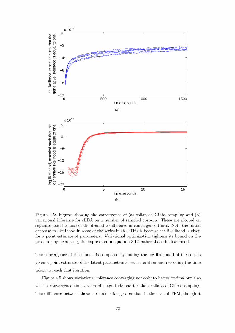


![A Survey of Text Mining Techniques and Applications · Text mining [1] is similar to data mining, except that data mining tools [2] are designed to handle structured data from databases](https://static.documents.pub/doc/80x56/5f53bcf4618636597671add2/a-survey-of-text-mining-techniques-and-text-mining-1-is-similar-to-data-mining.jpg)


