64


Mixed Finite Element Methods for Addressing Multi-Species
Diffusion Using the Stefan-Maxwell Equations
Mike McLeod
Thesis submitted to the Faculty of Graduate and Postdoctoral Studies
in partial fulfillment of the requirements for the degree of Master of Science in
Mathematics 1
Department of Mathematics and Statistics
Faculty of Science
University of Ottawa
c⃝ Mike McLeod, Ottawa, Canada, 2013
1The M.Sc. program is a joint program with Carleton University, administered by the Ottawa-Carleton Institute of Mathematics and Statistics
Abstract
The Stefan-Maxwell equations are a system of nonlinear partial differential equations
that describe the diffusion of multiple chemical species in a container. These equations
are of particular interest for their applications to biology and chemical engineering.
The nonlinearity and coupled nature of the equations involving many variables make
finding solutions difficult, so numerical methods are often used. In the engineering
literature the system is inverted to write fluxes as functions of the species gradient
before any numerical method is applied. In this thesis it is shown that employing a
mixed finite element method makes the inversion unnecessary, allowing the numerical
solution of Stefan-Maxwell equations in their primitive form. The plan of the thesis is
as follows, first a mixed variational formulation will be derived for the Stefan-Maxwell
equations. The nonlinearity will be dealt with through a linearization. Conditions for
well-posedness of the linearized formulation are then determined. Next, the linearized
variational formulation is approximated using mixed finite element methods. The
finite element methods will then be shown to converge to an approximate solution. A
priori error estimates are obtained between the solution to the approximate problem
and the exact solution. The convergence order is then verified through an analytic
test case and compared to standard methods. Finally, the solution is computed
for another test case involving the diffusion of three species and compared to other
methods.
ii

Acknowledgements
I would like to thank my supervisor Professor Yves Bourgault for his guidance through-
out the entire project. It has been immensely helpful in making me a better mathe-
matician.
I want to thank my mom for supporting me throughout my education and for con-
stantly talking science with me.
And I want to thank Katie for her constant love and support. You’re awesome and I
love you.
To everyone else who made this possible, thank you.
iii
Contents
1 Introduction 1
1.1 Stefan-Maxwell Equations . . . . . . . . . . . . . . . . . . . . . . 1
1.2 Mixed Variational Formulations . . . . . . . . . . . . . . . . . . 3
1.3 Literature Review . . . . . . . . . . . . . . . . . . . . . . . . . . 5
1.4 Outline of the Thesis . . . . . . . . . . . . . . . . . . . . . . . . 7
2 Mixed Variational Formulation of Stefan-Maxwell Equations 8
2.1 Variational Formulation . . . . . . . . . . . . . . . . . . . . . . . 8
2.2 Existence and Uniqueness for the Linearized Ternary Stefan-
Maxwell Equations . . . . . . . . . . . . . . . . . . . . . . . . . . 13
3 Numerical Analysis 25
3.1 Discretization of Stefan-Maxwell Equation . . . . . . . . . . . . . 25
3.2 Finite Element Spaces . . . . . . . . . . . . . . . . . . . . . . . . 27
3.3 Stability and Convergence of the Finite Element Method . . . . . 30
3.4 Standard Finite Element Methods . . . . . . . . . . . . . . . . . 32
4 Numerical Results 35
4.1 Implementation of the Mixed Finite Element Method . . . . . . 35
4.2 Analytic Test Case . . . . . . . . . . . . . . . . . . . . . . . . . . 36
4.3 Mazumder Test Case . . . . . . . . . . . . . . . . . . . . . . . . 45
iv
CONTENTS v
5 Conclusion 53
5.1 Contribution of this Thesis . . . . . . . . . . . . . . . . . . . . . 53
5.2 Future Work . . . . . . . . . . . . . . . . . . . . . . . . . . . . . 55
Bibliography 58
Chapter 1
Introduction
1.1 Stefan-Maxwell Equations
The Stefan-Maxwell equations describe the process of diffusion in a mixture of mul-
tiple chemical species. They were developed independently by Maxwell and Stefan
and serve as a generalization of other diffusion laws. Simpler diffusion models such
as Fick’s Law [15] have been shown by Duncan and Toor to give inaccurate results
in ternary mixtures [11]. Therefore the Stefan-Maxwell equations are preferred. The
Stefan-Maxwell equations have applications to biology and chemical engineering. A
simple derivation of the equations is presented here. A more detailed discussion of
the physics behind the Stefan-Maxwell equations can be found in [15] or [22].
Physically the system represents a mixture of n ideal gases, where each species i
has a mole fraction of ξi, in moles per unit volume, and a flux of Ji, in moles per unit
area per unit of time. If the mixture reaches steady state, the divergence of the flux
will be equal to some reaction rate ri. This leads to the following: For i = 1, 2, ..., n:
∇ · Ji = ri.
The motion of the gases will cause the particles of one species to be dragged by
the particles of the other species in the mixture. This drag force is balanced by the
1
1. Introduction 2
partial pressure gradients of the species in the mixture. This leads to the following
expression for i = 1, 2, ..., n:
−∇ξi =1
ctot
n∑j=1
ξjJi − ξiJjDij
,
where Dij is the binary diffusion coefficient between species i and species j, and
ctot > 0 is the total concentration of the mixture. The coefficients Dij and Dji are
taken to be equal [15].
Consider a domain Ω ⊂ Rd, such that the boundary of Ω ,Γ, is divided into two
components, ΓD and ΓN . These components satisfy: ΓD
∩ΓN = ∅. On the boundary
ΓD, the molar fraction ξi is taken to be fi. On ΓN , with outward unit normal vector
ν, the normal flux of species i, Ji ·ν, is taken to be gi. Since the variable ξi represents
mole fractions, at any point in the domain the following condition holds:
n∑i=1
ξi = 1.
To define the full system we will make use of the following fact in [3, 16]:
n∑i=1
Ji = 0.
We will use the following definitions:
ξ = (ξ1, ξ2, ..., ξn),
J = (J1, J2, ..., Jn).
The Stefan Maxwell problem for steady n-ary diffusion becomes: Find (J, ξ) such
that the following equations are satisfied in Ω for i = 1, 2, ..., n:
−∇ξi =1
ctot
n∑j=1
ξjJi − ξiJjDij
, (1.1.1)
1. Introduction 3
∇ · Ji = ri, (1.1.2)n∑
i=1
ξi = 1, (1.1.3)
n∑i=1
Ji = 0, (1.1.4)
with the following boundary conditions on Γ:
ξi = fi on ΓD, (1.1.5)
Ji · ν = gi on ΓN . (1.1.6)
Remark: If all of the binary diffusion coefficients are taken to be equal to a
value D, then the Stefan-Maxwell equations become:
Ji = −D∇ξi, for i = 1, 2, ..., n. (1.1.7)
This equation is referred to as Fick’s Law[15, 22].
The nonlinearity and the coupling terms in the Stefan-Maxwell equations make
finding analytic solutions difficult or impossible, therefore numerical methods are
necessary. In this thesis numerical solutions are found using mixed finite element
methods. To set up the numerical method we need to establish a mixed variational
formulation for the Stefan-Maxwell equations.
1.2 Mixed Variational Formulations
In this section mixed variational formulations are introduced by their application
to the Poisson problem. The difference between a mixed variational formulation
and a standard formulation, is that the mixed formulation solves for two variables
simultaneously. A detailed look at mixed formulations can be found in [7, 20].
1. Introduction 4
The Poisson problem is as follows: Find a function u in the domain Ω ⊂ Rn such
that:
− u = r on Ω,
u = f on Γ.
where Γ is the boundary of Ω.
To obtain the mixed formulation we make the following definition:
p = ∇u.
We can now rewrite the Poisson equation as follows:
p−∇u = 0 in Ω,
∇ · p = −r in Ω.
To find weak solutions of the above system, we multiply the first equation by
a vectorial test function q, and the second equation by a scalar test function v. We
then integrate both equations over the domain Ω. Finding weak solutions of the
above differential equations is now a matter of solving the following problem: Find
(p, u) ∈ Q× V satisfying:
∫Ω
(p · q + u∇ · q) dx =
∫Γ
fq · ν ds,∫Ω
v∇ · p dx = −∫Ω
rv dx,
where ν is the outward unit normal vector to the boundary Γ.
To complete the mixed variational formulation we need to identify the spaces Q
and V. In order for the above integrals to be defined, we require that the divergence
of the functions p and q are in L2(Ω). Therefore the space Q will be defined as:
1. Introduction 5
H(div; Ω) = q ∈ (L2(Ω))n| ∇ · q ∈ L2(Ω), (1.2.1)
and V will be taken to be L2(Ω). Take r ∈ L2(Ω) so that the integral in the right-
hand side of the second equation is well-defined. The function f will be taken to be
in H1/2(Ω) so the boundary integral in the first equation is understood as the duality
product of q · ν ∈ H−1/2(Γ) with f ∈ H1/2(Γ), see [23, p. 9]:
∫Γ
fq · νds :=< q · ν, f >H−1/2(Γ)×H1/2(Γ) .
This and related operators will be defined below.
The formulation above is now our mixed formulation for the Poisson equation.
It allows us to solve simultaneously for both u and its gradient p.
The Stefan-Maxwell equations naturally lead to a mixed variational formulation
where u stands for molar fractions and p represents the fluxes. Surprisingly enough,
such a formulation and related mixed finite element methods have not yet been pro-
posed for the Stefan-Maxwell equations, at least not that we know of.
1.3 Literature Review
The Stefan-Maxwell equations can be found in applications throughout the chemical
engineering literature. The usual method for finding a numerical solution is to invert
the system and apply the finite element method. In [1] a model for bone tissue
growth using coupled Navier-Stokes and Stefan-Maxwell equations is described. The
authors invert the Stefan-Maxwell equations to express the fluxes in terms of mass
fractions before applying a finite element method using the finite element software
Femlab. In [4] a benchmark for diffusion and fluid flow is introduced. The model
used relies on an inversion of the Stefan-Maxwell equations before applying a finite
element method to find the solution. A model of water transport in a fuel cell is
1. Introduction 6
described in [14] using Stefan-Maxwell and concentrated solution theory. The flux of
water at the membrane is determined using concentrated solution theory. The fluxes
are expressed in terms of the mass fractions before applying a finite element method,
except on the boundary where normal fluxes are used as boundary conditions. The
stability of the finite element scheme for Stefan-Maxwell equations is considered in
[17]. The system is inverted so that the flux is written explicitly in terms of the mass
fractions before any finite element scheme is applied. A finite volume approach is
applied in [18] where the flux is written in a discretized form using what the authors
refer to as a “coupled exponential scheme”.
Less often a finite difference scheme is used to numerically solve the Stefan-
Maxwell equations. In [9] a finite difference scheme for the mole fractions and veloc-
ities is used to approximate the gradients of the mole fractions. The molar flux is
expressed in terms of the velocities and mole fractions and solutions are found using
a 4th order Runge-Kutta scheme. A 1D problem is considered in [16] to study the
phenomena of uphill diffusion. The Stefan-Maxwell equations are solved using a finite
difference discretization, and the numerical method is shown to be second order and
a condition for L∞-stability is found.
Recently work has been done looking at the mathematical properties of Stefan-
Maxwell equations [3, 16]. In [16] conditions are imposed which show that if the initial
functions ξini are nonnegative functions in L∞(Ω) then the Stefan-Maxwell equations
admit unique smooth solutions for all time, moreover ξi remains nonnegative. It has
been shown in [3] that the time dependent homogenous system is well-posed for a
solution that is local in time. Additionally the same paper has shown that the mole
fractions ξi are non-negative for the inhomogenous case, under certain conditions on
the reaction rates. A main piece of the argument in both proofs is that the system is
invertible for each Ji as a function of ∇ξj.
There has been, until now, no work done on the Stefan-Maxwell equations in the
context of mixed finite element methods. The system of equations naturally leads to
1. Introduction 7
a mixed formulation. In this thesis, mixed finite element methods will be developed
and applied to the Stefan-Maxwell equations and compared to previous work done.
1.4 Outline of the Thesis
The thesis is orgranized in the following way. In the second chapter a mixed varia-
tional formulation of the Stefan-Maxwell equations is found and conditions for well-
posedness are determined in the case of ternary diffusion. In the third chapter the
ternary mixed variational formulation is discretized using mixed finite element meth-
ods. The method is then shown to converge to a solution of the Stefan-Maxwell
problem and error estimates between the approximate finite element solution and the
exact solution are found. In the fourth chapter, numerical test cases are presented.
The first test case is used to verify the error estimates found in chapter three and
to be used for comparison to standard methods. Numerical solutions are then found
using mixed finite element methods for two other test cases and are compared to
solutions obtained with other methods.
Chapter 2
Mixed Variational Formulation of
Stefan-Maxwell Equations
In this chapter a mixed variational formulation will be proposed to obtain a weak
solution to the Stefan-Maxwell equations. After the problem is set up, the existence
of a solution for a linearized problem will be analyzed using standard theory for
abstract saddle point problems.
2.1 Variational Formulation
We first establish a mixed variational formulation of the Stefan Maxwell equations
given in equations (1.1.1)-(1.1.6).
By looking at the equations we can see that the Stefan-Maxwell equations form
a degenerate system. The degeneracy can be removed if equations (1.1.3) and (1.1.4)
are used to reduce the system to n− 1 species. For i = 1, 2, ..., n− 1, we can do the
reduction as follows:
−∇ξi =1
ctot
n−1∑j=1
(ξjJi − ξiJj
Dij
)+ξnJi − ξiJnctotDin
8
2. Mixed Variational Formulation of Stefan-Maxwell Equations 9
=n−1∑j=1
(ξjJi − ξiJjctotDij
)+
(1− ξ1 − ξ2 − ...− ξn−1) Ji + ξi (J1 + J2 + ...+ Jn−1)
ctotDin
=Ji
ctotDin
+1
ctot
n−1∑j=1
(1
Dij
− 1
Din
)(ξjJi − ξiJj)
Define the following coefficients for i, j = 1, 2, ..., n− 1:
αij =1
Din
− 1
Dij
. (2.1.1)
The above equation can be stated as:
−∇ξi =Ji
ctotDin
+1
ctot
n−1∑j=1
αij (ξiJj − ξjJi) (2.1.2)
The molar fraction variable, now defined as ξ = (ξ1, ..., ξn−1), is taken to be in
(L2(Ω))n−1. For the rest of the thesis we will use the following definition:
V := (L2(Ω))n−1. (2.1.3)
Before we derive the weak formulation, some preliminary spaces will be defined.
To enforce the boundary condition on ΓN , we need to ensure that it is possible to
define an operator which outputs the normal component of a vectorial function on
the boundary. This will allow us to embed the boundary condition into the functional
space to which J belongs.
To start, we define the trace operator:
Theorem 2.1.1. ([20],page 10) Let Ω be an open bounded set of RN with Lipschitz
continuous boundary Γ, and let s > 1/2. There exists a unique linear continuous map
γ, called the trace operator:
γ : Hs(Ω) → Hs−1/2(Ω),
such that,
γ(q) := q|Γ ∀q ∈ Hs(Ω) ∩ C0(Ω).
2. Mixed Variational Formulation of Stefan-Maxwell Equations 10
We shall use this trace operator to define a normal trace operator.
Theorem 2.1.2. ([20], page 10) Let Ω be an open bounded set with a Lipschitz bound-
ary Γ. Then there exists a linear continuous operator γν ∈ L(H(div; Ω), H−1/2(Γ)
)such that
γν(q) := q · ν|Γ ∀q ∈ C∞(Ω). (2.1.4)
Definition 2.1.3. Let Ω be Lipschitz domain with boundary Γ and ΓN ⊂ Γ. Then
the restriction γν,ΓN(q) of γν(q) to ΓN is defined as follows:
< γν,ΓN(q), γ(Φ) >H−1/2(ΓN )×H1/2(ΓN )=< γν(q), γ(Φ) >H−1/2(Γ)×H1/2(Γ), (2.1.5)
for all Φ ∈ H1(Ω) with Φ = 0 on Γ/ΓN .
From (2.1.4) we have:
γν,ΓN(q) = q · ν|ΓN
∀q ∈ C∞(Ω). (2.1.6)
So the flux variable will be taken in the following space:
Q = q ∈ (L2(Ω))n−1|∇ · qi ∈ L2(Ω). (2.1.7)
If we enforce boundary conditions on the normal flux we will use the following
functional space for J :
Qg = q ∈ (L2(Ω))n−1|∇ · qi ∈ L2(Ω); γν,ΓN(qi) = gi on ΓN, (2.1.8)
where gi ∈ H−1/2(ΓN) are given for i = 1, ..., n− 1. We define Q0 in a similar fashion
where γν,ΓN(qi) = 0.
To simplify our notation we write:
< q · ν,Φ >ΓN:=< γν,ΓN
(q), γ(Φ) >H−1/2(ΓN )×H1/2(ΓN ), (2.1.9)
2. Mixed Variational Formulation of Stefan-Maxwell Equations 11
and similarly on Γ and ΓD.
To put these equations into a variational form, we multiply (2.1.2) by a test
function qi, where q = (q1, ..., qn−1) ∈ Q0, and multiply the reaction equation (1.1.2)
by a test function vi where v = (v1, ..., vn−1) ∈ V , then integrate both equations over
the domain Ω. For i = 1, 2, ...n− 1 we get:
∫Ω
−∇ξi · qi dx =
∫Ω
1
ctot
(Ji · qiDin
+n−1∑j=1
αij (ξiJj · qi − ξjJi · qi)
)dx,∫
Ω
vi∇ · Ji dx =
∫Ω
rivi dx.
By applying integration by parts, the gradient term on each ξi can be removed
at the cost of a term on the boundary:
− < qi · ν, ξi >Γ +
∫Ω
ξi∇ · qi dx =
∫Ω
1
ctot
(Ji · qiDin
+n−1∑j=1
αij (ξiJj · qi − ξjJi · qi)
)dx.
Since the test function qi is in the space Q0 the boundary term vanishes on ΓN .
This leaves the following equations for i = 1, 2, ..., n− 1:
− < qi ·ν, ξi >ΓD+
∫Ω
ξi∇· qi dx =
∫Ω
1
ctot
(Ji · qiDin
+n−1∑j=1
αij (ξiJj · qi − ξjJi · qi)
)dx.
To enforce the condition on ΓD we substitute ξi with fi in the boundary term.
To ensure the duality product is well defined, fi will be taken in H1/2(ΓD). We
are left with the following mixed variational formulation: Given fi ∈ H1/2(ΓD) and
ri ∈ L2(Ω) find (J, ξ) ∈ Qg × V such that:
∫Ω
(Ji · qictotDin
+n−1∑j=1
αij
ctot(ξiJj · qi − ξjJi · qi) − ξi∇ · qi
)dx = − < qi · ν, fi >ΓD
,
(2.1.10)
2. Mixed Variational Formulation of Stefan-Maxwell Equations 12
∫Ω
vi∇ · Ji dx =
∫Ω
rivi dx, (2.1.11)
for i = 1, 2, ..., n− 1 and ∀q = (q1, q2, ..., qn−1) ∈ Q0, ∀ v = (v1, v2, ..., vn−1) ∈ V .
It will be useful to know what conditions ensure that a solution to the variational
formulation is also a solution to the Stefan-Maxwell equations. We will make use of
D(Ω), the space of infinitely differentiable functions with compact support on Ω.
Now let (J, ξ) ∈ Qg×V be a solution to the above mixed variational formulation. By
rearranging (2.1.11) in the formulation we get the following equality for all vi ∈ L2(Ω):
∫Ω
(∇ · Ji − ri)vi dx = 0.
Since Ji ∈ H(div; Ω), we know that ∇ · Ji is an L2-function. By taking vi ∈
D(Ω) ⊂ L2(Ω) we recover ∇·Ji = ri in the sense of distributions and since both sides
of this equality are in L2(Ω), the equation is true almost everywhere on Ω.
To recover the rest of the Stefan-Maxwell problem we consider:∫Ω
(Ji · qictotDin
+n−1∑j=1
αij
ctot(ξiJj · qi − ξjJi · qi) − ξi∇ · qi
)dx+ < qi · ν, fi >ΓD
= 0.
If we assume that ξi ∈ H1(Ω) then we can apply integration by parts to the ξi∇ · qiterm and get:
0 =
∫Ω
(Ji · qictotDin
+n−1∑j=1
αij
ctot(ξiJj · qi − ξjJi · qi) +∇ξi · qi
)dx
− < qi · ν, ξi >Γ + < qi · ν, fi >ΓD
=
∫Ω
(Ji
ctotDin
+n−1∑j=1
αij
ctot(ξiJj − ξjJi) +∇ξi
)· qi dx
− < qi · ν, ξi >ΓN+ < qi · ν, fi − ξi >ΓD
The above equation is true for all qi ∈ H(div; Ω), so take qi ∈ (D(Ω))d ⊂
H(div; Ω). Since qi vanishes on Γ we recover equation (2.1.2) in the sense of distribu-
tions. To recover the boundary conditions, take qi equal to zero on ΓN . This choice
2. Mixed Variational Formulation of Stefan-Maxwell Equations 13
of qi is possible due to the surjectivity of the γν,ΓNoperator. For this choice of qi we
obtain that:
< qi · ν, fi − ξi >ΓD= 0 ∀q · ν ∈ H−1/2(ΓD),
which implies that fi = ξi in H1/2(ΓD). Since H
1/2(ΓD) ⊂ L2(ΓD), we get that fi = ξi
almost everywhere on ΓD. The boundary condition on the normal flux of J is satisfied
in H−1/2(ΓN) since it belongs to Qg.
So a solution to the mixed variational formulation with ξ ∈ (H1(Ω))2 and Ji ∈
H(div; Ω), will also be a solution to the Stefan-Maxwell problem.
2.2 Existence and Uniqueness for the Linearized
Ternary Stefan-Maxwell Equations
In this section the Stefan-Maxwell problem is analyzed using the theory for mixed
variational formulations, often referred to as abstract saddle point problems. This
theory will be briefly reviewed here, and is based on [7, Ch. II] . Following this review,
the general theory will be applied to the case of ternary diffusion.
Take V and Q to be Hilbert spaces with inner products (·, ·)V and (·, ·)Q, respec-
tively, and their associated norms defined as || · ||V and || · ||Q. Define two bounded
bilinear forms a(·, ·) : Q×Q→ R and b(·, ·) : Q× V → R. The abstract saddle point
problem is stated as follows: Given f ∈ Q∗ and r ∈ V ∗ find (J, ξ) ∈ Q×V such that:
a(J, q) + b(q, ξ) =< f, q >Q∗×Q ∀q in Q, (2.2.1)
b(J, v) = < r, v >V ∗×V , ∀v in V, (2.2.2)
where V ∗ and Q∗ are taken to be the dual spaces of V and Q with < ·, · > denoting the
duality product between the subscripted spaces. The saddle point formulation can be
2. Mixed Variational Formulation of Stefan-Maxwell Equations 14
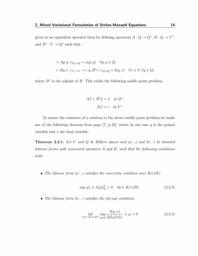
given in an equivalent operator form by defining operators A : Q→ Q∗, B : Q→ V ∗,
and B∗ : V → Q∗ such that :
< Ap, q >Q∗×Q = a(p, q) ∀p, q ∈ Q,
< Bq, v >V ∗×V =< q,B∗v >Q×Q∗= b(q, v) ∀v ∈ V, ∀q ∈ Q,
where B∗ is the adjoint of B. This yields the following saddle point problem:
AJ +B∗ξ = f in Q∗,
BJ = r in V ∗.
To ensure the existence of a solution to the above saddle point problem we make
use of the following theorem from page [7, p.42]; where in our case q is the primal
variable and v the dual variable:
Theorem 2.2.1. Let V and Q be Hilbert spaces and a(·, ·) and b(·, ·) be bounded
bilinear forms with associated operators A and B, such that the following conditions
hold:
• The bilinear form a(·, ·) satisfies the coercivity condition over Ker(B):
a(p, p) ≥ λ||p||2Q > 0 ∀p ∈ Ker(B). (2.2.3)
• The bilinear form b(·, ·) satisfies the inf-sup condition:
infv∈V \Ker(B∗)
supq∈Q
b(q, v)
∥q∥Q∥v∥V≥ µ > 0 (2.2.4)
2. Mixed Variational Formulation of Stefan-Maxwell Equations 15
Then for any f ∈ V ∗ and r ∈ Im(B), the saddle point problem equations (2.2.1)-
(2.2.2) admits a solution (J, ξ) ∈ Q × V where J ∈ Q is uniquely determined and
ξ ∈ V is unique up to an element of Ker(B∗).
Proof: For a proof see [7, Ch.II].
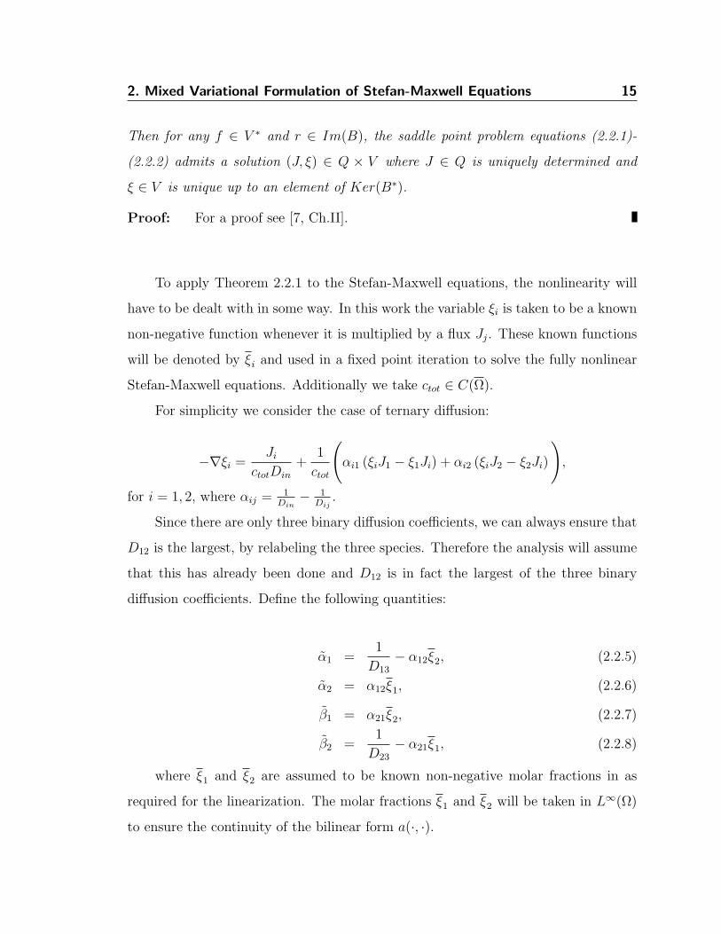
To apply Theorem 2.2.1 to the Stefan-Maxwell equations, the nonlinearity will
have to be dealt with in some way. In this work the variable ξi is taken to be a known
non-negative function whenever it is multiplied by a flux Jj. These known functions
will be denoted by ξi and used in a fixed point iteration to solve the fully nonlinear
Stefan-Maxwell equations. Additionally we take ctot ∈ C(Ω).
For simplicity we consider the case of ternary diffusion:
−∇ξi =Ji
ctotDin
+1
ctot
(αi1 (ξiJ1 − ξ1Ji) + αi2 (ξiJ2 − ξ2Ji)
),
for i = 1, 2, where αij =1
Din− 1
Dij.
Since there are only three binary diffusion coefficients, we can always ensure that
D12 is the largest, by relabeling the three species. Therefore the analysis will assume
that this has already been done and D12 is in fact the largest of the three binary
diffusion coefficients. Define the following quantities:
α1 =1
D13
− α12ξ2, (2.2.5)
α2 = α12ξ1, (2.2.6)
β1 = α21ξ2, (2.2.7)
β2 =1
D23
− α21ξ1, (2.2.8)
where ξ1 and ξ2 are assumed to be known non-negative molar fractions in as
required for the linearization. The molar fractions ξ1 and ξ2 will be taken in L∞(Ω)
to ensure the continuity of the bilinear form a(·, ·).
2. Mixed Variational Formulation of Stefan-Maxwell Equations 16
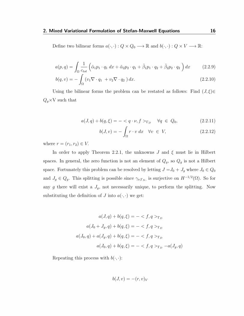
Define two bilinear forms a(·, ·) : Q×Q0 −→ R and b(·, ·) : Q× V −→ R:
a(p, q) =
∫Ω
1
ctot
(α1p1 · q1 dx+ α2p2 · q1 + β1p1 · q2 + β2p2 · q2
)dx (2.2.9)
b(q, v) = −∫Ω
(v1∇ · q1 + v2∇ · q2 ) dx. (2.2.10)
Using the bilinear forms the problem can be restated as follows: Find (J, ξ)∈
Qg×V such that
a(J, q) + b(q, ξ) = − < q · ν, f >ΓD∀q ∈ Q0, (2.2.11)
b(J, v) = −∫Ω
r · v dx ∀v ∈ V, (2.2.12)
where r = (r1, r2) ∈ V.
In order to apply Theorem 2.2.1, the unknowns J and ξ must lie in Hilbert
spaces. In general, the zero function is not an element of Qg, so Qg is not a Hilbert
space. Fortunately this problem can be resolved by letting J =J0 + Jg where J0 ∈ Q0
and Jg ∈ Qg. This splitting is possible since γν,ΓN , is surjective on H−1/2(Ω). So for
any g there will exist a Jg, not necessarily unique, to perform the splitting. Now
substituting the definition of J into a(·, ·) we get:
a(J, q) + b(q, ξ) = − < f, q >ΓD
a(J0 + Jg, q) + b(q, ξ) = − < f, q >ΓD
a(J0, q) + a(Jg, q) + b(q, ξ) = − < f, q >ΓD
a(J0, q) + b(q, ξ) = − < f, q >ΓD−a(Jg, q)
Repeating this process with b(·, ·):
b(J, v) = −(r, v)V
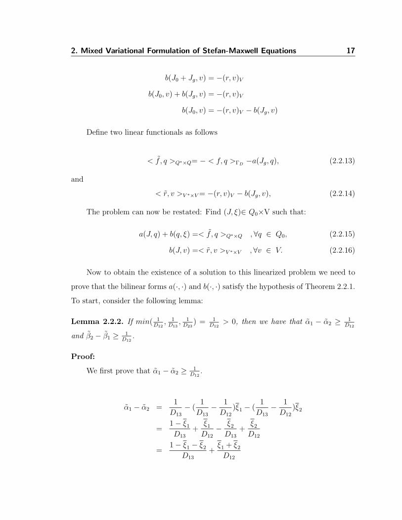
2. Mixed Variational Formulation of Stefan-Maxwell Equations 17
b(J0 + Jg, v) = −(r, v)V
b(J0, v) + b(Jg, v) = −(r, v)V
b(J0, v) = −(r, v)V − b(Jg, v)
Define two linear functionals as follows
< f, q >Q∗×Q= − < f, q >ΓD−a(Jg, q), (2.2.13)
and
< r, v >V ∗×V= −(r, v)V − b(Jg, v), (2.2.14)
The problem can now be restated: Find (J, ξ)∈ Q0×V such that:
a(J, q) + b(q, ξ) =< f, q >Q∗×Q , ∀q ∈ Q0, (2.2.15)
b(J, v) =< r, v >V ∗×V , ∀v ∈ V. (2.2.16)
Now to obtain the existence of a solution to this linearized problem we need to
prove that the bilinear forms a(·, ·) and b(·, ·) satisfy the hypothesis of Theorem 2.2.1.
To start, consider the following lemma:
Lemma 2.2.2. If min( 1D12
, 1D13
, 1D23
) = 1D12
> 0, then we have that α1 − α2 ≥ 1D12
and β2 − β1 ≥ 1D12
.
Proof:
We first prove that α1 − α2 ≥ 1D12
.
α1 − α2 =1
D13
− (1
D13
− 1
D12
)ξ1 − (1
D13
− 1
D12
)ξ2
=1− ξ1D13
+ξ1D12
− ξ2D13
+ξ2D12
=1− ξ1 − ξ2
D13
+ξ1 + ξ2D12
2. Mixed Variational Formulation of Stefan-Maxwell Equations 18
≥ 1− ξ1 − ξ2D12
+ξ1 + ξ2D12
=1
D12
Now to prove the other inequality, we proceed in much the same way:
β2 − β1 =1
D23
− (1
D23
− 1
D12
)ξ2 − (1
D23
− 1
D12
)ξ1
=1− ξ2D23
+ξ2D12
− ξ1D23
+ξ1D12
=1− ξ1 − ξ2
D23
+ξ1 + ξ2D12
≥ 1− ξ1 − ξ2D12
+ξ1 + ξ2D12
=1
D12
We have used the fact that the ξi’s add up to one and that the binary diffusion
coefficient D12 is the largest.
We now consider the continuity and coercivity of a(·, ·) with the following propo-
sition:
Proposition 2.2.3. If the binary diffusion coefficients satisfy 3D23 > D12 and 3D13 >
D12, then the bilinear form a(·, ·) is coercive and continuous.
Proof: We rewrite the bilinear form in the following way:
a(p, q) =
∫Ω
1
ctot
2∑i=1
(qi1, q
i2
) α1 α2
β1 β2
pi1
pi2
dx
Since ctot > 0 in Ω, there exist values cmin and cmax such that 0 < cmin ≤ ctot ≤
cmax everywhere in Ω. So when bounding the bilinear form from above or below, we
can use cmin or cmax and ignore ctot.
2. Mixed Variational Formulation of Stefan-Maxwell Equations 19
To start we consider the coercivity of a(·, ·). The bilinear form is coercive if
and only if the symmetric part of the matrix is positive definite with the smallest
eigenvalue uniformly bounded away from 0 for all ξi. So to prove the coercivity we
will consider:
Asym =
α1α2+β1
2
α2+β1
2β2
.
Positive definiteness of the matrix will be established by showing that the matrix
has strictly positive eigenvalues. To do this we apply the Gershgorin circle theorem
to find lower bounds on the eigenvalues of Asym.
We now consider the Gershgorin circle for the first row:
2α1 − (α2 + β1) ≥ 2α1 − (α1 −1
D12
+ β1)
=1
D13
− α12ξ2 − α21ξ2 +1
D12
=1
D13
−(
1
D13
− 1
D12
)ξ2 −
(1
D23
− 1
D12
)ξ2 +
1
D12
=1− ξ2D13
+ 2ξ2D12
− ξ2D23
+1
D12
where the inequality comes from applying Lemma 2.2.2.
This last line is a linear equation in ξ2, so for ξ2 ∈ [0, 1] the minimum value will
be achieved at one of the interval end points. Therefore we get:
2α1 − (α2 + β1) ≥ min 1
D13
+1
D12
,3
D12
− 1
D23
> 0,
where the positivity comes from the assumption that 3D23 > D12.
Now consider the other Gershgorin circle:
2β2 − (α2 + β1) ≥ 2β2 − (α2 + β2 −1
D12
)
2. Mixed Variational Formulation of Stefan-Maxwell Equations 20
=1
D23
− α21ξ1 − α12ξ1 +1
D12
=1
D23
−(
1
D23
− 1
D12
)ξ1 −
(1
D13
− 1
D12
)ξ1 +
1
D12
=1− ξ1D23
+ 2ξ1D12
− ξ1D13
+1
D12
.
As before the last line is a linear equation in ξ1. So we get:
2β2 − (α2 + β1) ≥ min 1
D23
+1
D12
,3
D12
− 1
D13
> 0,
here the positivity comes from the assumption that 3D13 > D12.
By the Gershgorin theorem the matrix has positive eigenvalues, so we can con-
clude that it is in fact positive definite.
To prove the continuity of a(·, ·) we only need to show that the operator A is
bounded [2, pg. 334]. Therefore we need to show that ||Av||V ∗ ≤ C||v||V ∗. By
showing that the matrix Asym has uniformly bounded coefficients, we obtain that the
constant C in this inequality is finite. Since ξi ∈ [0, 1] the functions αi and βi are
bounded above by 1D13
and 1D23
respectively. By taking C = max 1D13
, 1D23
we get
that ||Av||V ∗ ≤ C||v||V ∗. Therefore we can conclude that a(p, q) is continuous.
To prove the inf-sup condition for b(·, ·) we will make use of the following lemma
from [20]:
Lemma 2.2.4. For any v ∈ L2(Ω) there exists p ∈ H(div; Ω) such that ∇ · p = −v
and that satisfies the following inequality:
||p||H(div;Ω) ≤(√
1 + C2Ω
)||v||L2(Ω),
where CΩ is the constant in the Poincare inequality for the domain Ω.
2. Mixed Variational Formulation of Stefan-Maxwell Equations 21
Proof: For a given v ∈ L2(Ω) consider the following variational problem: Find
ϕ ∈ H10 (Ω) such that:
∫Ω
∇ϕ · ∇ψ dx =
∫Ω
vψ dx ∀ψ ∈ H10 (Ω).
By the Lax-Milgram theorem for any v ∈ L2(Ω) there exists a unique ϕ ∈ H10 (Ω)
which satisfies the above variational equation. By taking the test function ψ equal to
ϕ, we get:
||∇ϕ||2L2(Ω) =
∫Ω
|∇ϕ|2 dx
=
∫Ω
vϕ dx
≤ ||v||L2(Ω)||ϕ||L2(Ω)
≤ CΩ||v||L2(Ω)||∇ϕ||L2(Ω)
=⇒ ||∇ϕ||L2(Ω) ≤ CΩ||v||L2(Ω)
Setting p = ∇ϕ and integrating by parts:
∫Ω
vψ dx =
∫Ω
p · ∇ψ dx
=< p · ν, ψ >Γ −∫Ω
ψ∇ · p dx
= −∫Ω
ψ∇ · p dx,
where the boundary term vanishes because ψ = 0 on Γ. Take ψ ∈ D(Ω) ⊂ H10 (Ω),
we get that ∇ · p = −v in D′(Ω). Combining the above results we get the following:
||p||2H(div;Ω) = ||p||2L2(Ω) + ||∇ · p||2L2(Ω)
≤ ||∇ϕ||2L2(Ω) + ||∇ · p||2L2(Ω)
2. Mixed Variational Formulation of Stefan-Maxwell Equations 22
= C2Ω||v||2L2(Ω) + ||v||2L2(Ω),
which immediately implies the desired result.
We can now prove the following proposition:
Proposition 2.2.5. The bilinear form b(·, ·) for the Stefan-Maxwell problem, satisfies
the following inf-sup condition:
infv∈V
supp∈Q
b(p, v)
||v||V ||p||Q≥ µ,
for some µ > 0.
Proof:
Let v1 and v2 be L2(Ω) functions such that ∇ · pi = vi, i = 1, 2, as in Lemma
2.2.4. Then we have:
b(p, v) =
∫Ω−v1∇ · p1 − v2∇ · p2 dx
||[v1, v2]||V
=||v1||2L2(Ω) + ||v2||2L2(Ω)√||v1||2L2(Ω) + ||v2||2L2(Ω)
=√
||v1||2L2(Ω) + ||v2||2L2(Ω)
≥
√(||p1||2H(div;Ω) + ||p2||2H(div;Ω)
) 1
1 + C2Ω
=1√
1 + C2Ω
||p||Q,
where the inequality comes from Lemma 2.2.4. This leads to the following:
supp∈Q
b(p, v)
||p||Q≥
∫Ω−v1∇ · p1 − v2∇ · p2 dx
||p||Q
2. Mixed Variational Formulation of Stefan-Maxwell Equations 23
≥ 1√1 + C2
Ω
||v||V
The above is equivalent to the proposition since 1√1+C2
Ω
> 0.
We can use the results in this section to prove the following theorem:
Theorem 2.2.6. There exists a unique solution (J, ξ) ∈ Qg×V to the mixed formula-
tion of the linearized Stefan-Maxwell equations, when the binary diffusion coefficients
satisfy 3D23 > D12 and 3D13 > D12.
Proof: By the application of Theorem 2.2.1 we have that there exists a solution
(J, ξ) ∈ Qg × V to the Stefan-Maxwell problem. Furthermore if J = J0 + Jg, then
J0 will be defined uniquely for a given Jg. Now consider two solutions to the Stefan-
Maxwell problem, (J1, ξ1) and (J2, ξ2). Let J = J1 − J2 and ξ = ξ1 − ξ2. We have
that J ∈ Q0 since J1 · ν = J2 · ν on ΓN and ξ = 0 on ΓD. So (J , ξ) ∈ Q0 × V is a
solution to:
a(J , q) + b(q, ξ) = 0 ,∀q ∈ Q0,
b(J , v) = 0 ,∀v ∈ V.
By taking q = J and v = ξ we can combine the above equations to get:
a(J , J) = 0.
The coerciveness of a(·, ·) implies that J = 0. The system is therefore equivalent
to:
b(q, ξ) = 0 , ∀q ∈ Q0.
Set qi ∈ (D(Ω))d ⊂ H(div; Ω). Then we have
0 =
∫Ω
ξi∇ · qi dx = − < ∇ξi, qi >D′(Ω)×D(Ω) .
2. Mixed Variational Formulation of Stefan-Maxwell Equations 24
Therefore we have that ∇ξi = 0 in D′(Ω). Since ξi is L2(Ω) we have that ξi
coincides almost everywhere with a constant function [5, Corollary 2.1, p.9]. Since ξ
is a constant function we have that ξi ∈ H1(Ω). Now for qi ∈ Q0 we get:
0 =
∫Ω
ξi∇ · qi dx
= −∫Ω
∇ξi · qi dx+ < qi · ν, ξi >Γ
=< qi · ν, ξi >ΓD,
for all q · ν ∈ H−1/2(ΓD). This implies that ξi = 0 in H1/2(ΓD), and since ξi is
constant, we obtain that ξi is zero everywhere on Ω.
Since J and ξ are zero we obtain the uniqueness of solutions to the linearized
Stefan-Maxwell problem.
Remark: In order to consider the fully nonlinear Stefan-Maxwell equations we
would need to consider a fixed point mapping from ξi to ξi and show that it converges
in some space. This was attempted using Sobolev embeddings, in particular the
Rellich-Kondrachov Theorem. However we were unable to make any progress as the
fixed point mapping was continuous but not compact.
Chapter 3
Numerical Analysis
The theory of mixed finite element methods is summarized here with an emphasis
on results that will be used to approximate the Stefan-Maxwell problem. In the first
section the general mixed finite element problem is stated as well as the main theorem
for solution existence. In the second section the finite element spaces that approxi-
mate the functional spaces of the continuous problem are stated. The final section
investigates the stability and the order of convergence for different finite element
spaces.
3.1 Discretization of Stefan-Maxwell Equation
The finite dimensional approximation of the Stefan-Maxwell problem (2.2.15)-(2.2.16)
is as follows: Find (Jh, ξh) ∈ Qh × Vh that satisfy the following:
a(Jh, qh) + b(qh, ξh) =< f, qh >Q∗,Q ∀qh ∈ Qh, (3.1.1)
b(Jh, vh) =< r, vh >V ∗,V ∀vh ∈ Vh, (3.1.2)
where Vh and Qh are finite dimensional subspaces of V and Q, respectively. The
bilinear forms above define two operators, Ah : Qh → Q∗h and Bh : Qh → V ∗
h . The
25
3. Numerical Analysis 26
operator Bh has a kernel defined as Ker(Bh) = qh ∈ Qh| Bhqh = 0 = qh ∈
Qh| b(qh, vh) = 0, ∀vh ∈ Vh.
The existence of a solution for the continuous problem does not imply the exis-
tence of a solution to the discrete problem. This is because, in general, the operator
Bh is not the restriction of B to Qh.
The existence of a solution for the mixed finite element method is established by
the following theorem from [7, p.60]:
Theorem 3.1.1. Let V and Q be Hilbert spaces and let a(·, ·) : Q × Q → R and
b(·, ·) : Q × V → R be bounded linear forms with associated operators A : Q 7→ Q∗
and B : Q 7→ V ∗.
Moreover let Vh ⊂ V and Qh ⊂ Q be finite dimensional subspaces and Ah : Qh →
Q∗h and Bh : Qh → V ∗
h the operators associated to the restriction of a(·, ·) and b(·, ·)
to their respective finite dimensional subspaces.
Now assume the following are satisfied for two constants λh and µh :
(i) The bilinear form a(·, ·)|Vh×Vhsatisfies the following coercivity condition on
Ker(Bh):
a(ph, ph) ≥ λh||ph||2Q > 0 ∀ph ∈ Ker(Bh). (3.1.3)
(ii) The bilinear form b(·, ·)|Vh×Qhsatisfies the following inf-sup condition:
infvh∈Vh\Ker(B∗
h)sup
qh∈Qh
b(qh, vh)
∥qh∥Q∥vh∥V≥ µh > 0. (3.1.4)
Then for any f ∈ Q∗ and r ∈ Im(B) the finite dimensional saddle point problem
has a solution (Jh, ξh) ∈ Qh × Vh, where Jh is uniquely determined and ξh is unique
up to an element of Ker(B∗h).
Proof:
Full proof can be found in [7, section 2.2].
3. Numerical Analysis 27
If the mixed finite element method converges and the constants λh = λ and
µh = µ are independent of h, then we have the following a priori error estimates:
||J − Jh||Q ≤ (1 +||a||λ
)(1 +||b||µ
) infqh∈Qh
||J − qh||Q +||b||λ
infvh∈Vh
||ξ − vh||V , (3.1.5)
||ξ − ξh||V ≤ (1 +||b||µ
) infvh∈Vh
||ξ − vh||V +||a||µ
infqh∈Qh
||J − qh||Q. (3.1.6)
Remark If Ker(Bh) ⊂ Ker(B), then we have the following error estimate:
||J − Jh||Q ≤ (1 +||a||λ
)(1 +||b||µ
) infqh∈Qh
||J − qh||Q. (3.1.7)
A proof of these error estimates and others can be found in [7, Sec 2.2].
3.2 Finite Element Spaces
In order to determine if a specific mixed finite element method satisfies the hypothesis
of Theorem 3.1.1, two finite dimensional approximations of the spaces V and Q need
to be specified on any mesh Th. For this paper the mesh Th will always be a regular
triangular mesh. This means that the domain Ω will be tesselated by triangles, such
that if any two triangles share an edge, then they share the entire edge. Individual
triangles in the mesh will be denoted by K. Let h = maxK∈Thhk, where hk is the
size of the element K.
The space V will be approximated with the finite dimensional space P kdc of piece-
wise polynomials of degree k, which are discontinuous on element boundaries. If
Pk(K) is taken to be the space of k-th degree polynomials on any element K, then
P kdc is defined as follows:
P kdc = vh ∈ (L2(Ω))2|vh|K ∈ (Pk(K))2 ∀K ∈ Th (3.2.1)
3. Numerical Analysis 28
For k > 0, if we enforce continuity across elements K of Th then we get the following
space:
P k = vh ∈ (C0(Ω))2 | vh|K ∈ (P(k))2 ∀K ∈ Th (3.2.2)
There exists an interpolation operator onto the space P kdc with the following
property from [20, p.90]:
Proposition 3.2.1. Let k be a nonnegative integer. The interpolation operator Πh :
V → P kdc satisfies the following error estimate for k ≥ 0:
∥v − Πhv∥2V ≤ chk+1|v|k+1,Ω ∀v ∈ (Hk+1(Ω))2, (3.2.3)
where |v|k+1,Ω is the Hk+1(Ω) seminorm.
The space Q will be approximated using the k-th order Raviart-Thomas finite
element, RT k. To construct the space we need the following definition:
Definition 3.2.2. A homogeneous polynomial is one where all non zero terms have
the same degree. The space of homogeneous polynomials of degree k will be denoted
by Pk.
Using homogeneous polynomials we will define the following space on an element
K:
RT k(K) = (Pk(K))2 +
x
y
Pk(K).
The degrees of freedom for RT k are chosen such that the normal component qh ·ν
is continuous across element edges. This is done in such a way as to ensure that the
element is a subspace of H(div; Ω). For k = 0, the degrees of freedom for q · ν are
taken at the mid-edges. For k ≥ 0, see [7] for details on how this is done. We can
3. Numerical Analysis 29
now define the Raviart-Thomas finite element space over the entire domain Ω. For
k ≥ 0:
RT k = qh ∈ (H(div; Ω))2| qh,i|K ∈ RT k(K), i = 1, 2, ∀K ∈ Th. (3.2.4)
The space H(div; Ω) can also be approximated with the Brezzi-Douglas-Marini
elements of order k + 1 [6]. The space BDMk+1 defined by:
BDMk+1 = qh ∈ (H(div; Ω))2| qh,i|K ∈ (P kdc(K))2, i = 1, 2, ∀K ∈ Th. (3.2.5)
The degrees of freedom for BDMk+1 finite element functions are chosen such that the
functions are in H(div; Ω). For triangular elements we have that RT 0 ⊂ BDM1 ⊂
RT 1 ⊂ BDM2 and so on.
The space RT k has an interpolation operator, τh, with the following property:
Proposition 3.2.3. Let v ∈ P kdc. There exists an interpolator τh : (H(div; Ω))2 →
RT k that satisfies the following properties:
(i)
∫Ω
vi∇ · (qi − τh(qi)) = 0, (3.2.6)
(ii) ||τh(q)||Q ≤ C∗||q||Q, (3.2.7)
for a constant C∗ independent of h.
The interpolator also satisfies the following error estimate for q ∈ (Hk+1(Ω))2 :
∥τh(q)− q∥Q ≤ Chk+1(|q|k+1,Ω +2∑
i=1
|div(qi)|k+1,Ω) (3.2.8)
Proof: See Sec 3.4.2 and 7.2.2 in [20].
These finite element spaces and their associated properties will be essential in
proving that the method converges. The properties of the interpolators will be nec-
essary for investigating the convergence order of the method.
3. Numerical Analysis 30
3.3 Stability and Convergence of the Finite Ele-
ment Method
To analyze the stability and convergence of mixed finite element methods, suitable
finite element space combinations must be chosen such that the coercivity and the
inf-sup conditions are satisfied. For this, we choose the RT k/P kdc or the BDM
k+1/P kdc
combinations for discretizing J and ξ, respectively. This choice of spaces has the
property that div(RT k) = div(BDMk+1)= P kdc. This means that the operator Bh is
just the restriction of B to the subspace RT k or BDMk+1. So the coercivity condition
on a(·, ·) over Ker(Bh) is implied by the coercivity condition over Ker(B). For the
rest of the convergence analysis, only the Raviart-Thomas space will be considered,
although the BDMk+1 analysis is very similar.
Lemma 3.3.1. Assume there exists a µ > 0 such that ∀v ∈ L2(Ω), ∃q ∈ Q, q = 0,
that satisfies the continuous inf-sup condition, equation (2.2.4). Now assume there
exists an operator τh : Q→ RT k such that:
(1)
∫Ω
vh∇ · (qi − τh(qi)) = 0 i = 1, 2, (3.3.1)
(2) ∥τh(q)∥Q ≤ C∗||q||Q, (3.3.2)
then the inf-sup condition for the discrete problem (3.1.4) is satisfied for a constant
independent of h.
Proof: See [7, Prop. 2.8, p. 58] or [20, Lemma 7.2.1, p. 235].
We can now prove the following proposition:
Proposition 3.3.2. If qi ∈ H(div; Ω)2, then the inf-sup condition for the discrete
problem (3.1.4) is satisfied for Qh = RT k and Vh = P kdc.
3. Numerical Analysis 31
Proof: By Theorem 2.2.1 there exists a µ such that ∀v ∈ V, ∃q ∈ Q, q = 0 that
satisfies the continuous inf-sup condition, equation (2.2.4). Since qi ∈ H(div; Ω)2,
by Proposition 3.2.3 there exists an operator τh : H(div; Ω)2 → RT k that satisfies
(3.2.5) and (3.2.6). Now we can apply Lemma 3.3.1 and conclude that the inf-sup
condition for the discrete problem (3.1.5) is satisfied for a constant independent of h.
We will conclude this section with the following theorem:
Theorem 3.3.3. Assume the binary diffusion coefficients satisfy 3D23 > D12 and
3D13 > D12. The mixed finite element method for the linearized Stefan-Maxwell
problem defined by (3.1.1)-(3.1.2) has a solution (Jh, ξh) ∈ RT k × P kdc, where Jh and
ξh are unique. Provided the solution (ξ, J) ∈ (Hk+1(Ω))2 × (Hk+1(Ω)2)2, then the
following error estimates are satisfied:
||ξ − ξh||V ≤ Chk+1(|ξ|k+1,Ω + |J |k+1,Ω + |div(J)|k+1,Ω), (3.3.3)
||J − Jh||V ≤ Chk+1(|J |k+1,Ω + |div(J)|k+1,Ω), (3.3.4)
where | · |k+1,Ω denotes the Hk+1 semi-norm over Ω.
Proof: By proposition 3.3.2 the discrete inf-sup condition is satisfied, and the
coercivity of the bilinear form a(·, ·) over RT k is established by the coercivity over
(H(div; Ω))2. Therefore by Theorem 3.1.1 we have the existence of a solution (Jh, ξh) ∈
RT k × P kdc.
Since Ker(Bh) ⊂ Ker(B) we have the following error estimates from (3.1.6) and
(3.1.7):
||ξ − ξh||V ≤ c1 infvh∈Pk
dc
||ξ − vh||V + c2 infqh∈RTk
||J − qh||Q,
||J − Jh||V ≤ c3 infqh∈RTk
||J − qh||Q,
where c1 = (1 + ||b||µ), c2 =
||a||µ, and c3 = (1 + ||a||
λ)(1 + ||b||
µ).
3. Numerical Analysis 32
We use the interpolation operator’s error estimate, (3.2.3), to get an error esti-
mate for ξ in terms of semi-norms.
infvh∈Pk
dc
||ξ − vh||V ≤ ||ξ − Πhξ||V
≤ chk+1|ξ|k+1,Ω ∀ξ ∈ (Hk+1(Ω))2,
with a constant c independant from h and ξ.
We proceed in the same way using the interpolator (3.2.7) to get an error estimate
for J in terms of the Hk+1 seminorm.
infqh∈RTk
||J − qh||Q ≤ ||J − τhJ ||Q
≤ Chk+1(|J |k+1,Ω + |div(J)|k+1,Ω),
where this holds for all ∀J ∈ (Hk+1(Ω))2)2. We can now substitute the estimates for
the infimums of the norms into the error estimates above to get equations (3.3.3) and
(3.3.4).
3.4 Standard Finite Element Methods
For the sake of completeness standard finite element methods are presented here. For
this, we make use of the following definition:
A =
α1 α2
β1 β2
where the terms in the matrix are defined by equations (2.2.5)-(2.2.8).
3. Numerical Analysis 33
By taking equation (1.1.1) and using equations (1.1.3) and (1.1.4), the three
species system is reduced to the following two species system:
−∇ξi =2∑
j=1
AijJj,
for i = 1, 2.
The fluxes can be expressed in terms of the mole fractions and their gradients
by inverting the equation above to give:
Ji = −2∑
j=1
A−1ij ∇ξj, (3.4.1)
for i = 1, 2.
By taking the divergence on both sides and applying equation (1.1.2), we obtain
the following for i = 1, 2:
−∇ · (2∑
j=1
A−1ij ∇ξj) = ri.
The variational formulation is obtained by multiplying the above by a test func-
tion ϕi and integrating by parts to remove the divergence term. For a Dirichlet
problem this yields the following variational formulation: Find ξ ∈ (H1(Ω))2 where
ξi = fi on Γ such that:
∫Ω
(2∑
j=1
A−1ij ∇ξj) · ∇ϕi dx =
∫Ω
riϕi dx, (3.4.2)
for all ϕi ∈ H10 (Ω) and i = 1, 2. Just like in the case of the mixed finite element
method, this problem is solved multiple times where the nonlinearity is resolved using
the fixed point ξh,i := σξh,i+(1−σ)ξh,i. The finite element space approximation will
use the continuous P k spaces for k ≥ 1. These finite element methods will be referred
to as “Standard P k”.
For these “Standard P k” methods the flux will be recovered by solving (3.4.2)
for ξ and using equation (3.4.1) to strongly recover the flux J. The flux component

3. Numerical Analysis 34
Ji will be approximated by the space P 2k ×P 2k for i = 1, 2 as this yielded the lowest
L2 error in the numerical tests described in the next chapter.
Chapter 4
Numerical Results
In this chapter the mixed finite element method is used to compute approximate
solutions to the Stefan-Maxwell equations. We first discuss the implementation of the
mixed finite element method using FreeFem++[13]. Three test cases are considered.
The first test case has a known analytic solution which is compared to the mixed finite
element solution and used to verify the error estimates from the previous section.
The second test case was initially proposed by Mazumder in [17], and its solution is
computed using the numerical scheme. The third case, proposed by Bottcher in [4],
is a variation of the Mazumder test case.
4.1 Implementation of the Mixed Finite Element
Method
The mixed finite element methods were implemented using the open source software
FreeFem++[13]. Computations were done using the 64-bit version of Ubuntu 12.10
on a computer with 9GBs of RAM and an Intel Core i7 processor.
The software was used to construct the meshes, to build the finite element func-
tions, and for plotting the solutions.
35
4. Numerical Results 36
A fixed point iteration was used to resolve the nonlinearity of the Stefan-Maxwell
equations. The ξi were initially taken to be zero everywhere in the domain, then the
linearized Stefan Maxwell problem was solved numerically using the direct solver,
UMFPACK. The solution ξh was compared to the initial guess ξh through a com-
putation of ||ξh − ξh||V . If the norm was greater than 10−10, the functions ξh,i were
updated using the following equation:
ξh,i = σξh,i + (1− σ)ξh,i, (4.1.1)
where σ ∈ [0, 1]. A σ value less than one represents an under-relaxation of the fixed
point and may be necessary to achieve convergence. The procedure is then repeated
using the new values for the ξi functions until the norm ||ξh− ξh||V is less than 10−10.
The fixed point iterations were then stopped and the solution (J, ξ) was plotted using
FreeFEM++’s built in plot function.
4.2 Analytic Test Case
A test case was constructed on a domain Ω with boundary conditions and reac-
tion rates such that the solution to the Stefan-Maxwell problem was known exactly.
The L2-error between the exact solution and the numerical approximation was then
computed for varying mesh sizes. This was then used to determine the order of
convergence of the mixed finite element methods.
We consider the domain Ω = [0, 1] × [0, 1] and proceed with the method of
manufactured solution where an analytical solution is provided and the data (right-
hand side and boundary condition) are adjusted so the Stefan-Maxwell problem is
satisfied. Define two functions f1 and f2 as follows:
4. Numerical Results 37
f1 =
sinh(π
2)sin(πx
2)
π2 x ∈ [0, 1], y = 1sinh(πy
2)
π2 x = 1, y ∈ [0, 1]
0 Otherwise
f2 =
cosh(π2)cos(πx
2)
π2 x ∈ [0, 1], y = 1cos(πx
2)
π2 x ∈ [0, 1], y = 0cosh(πy
2)
π2 x = 0, y ∈ [0, 1]
0 Otherwise
For this benchmark, Dirichlet boundary conditions are used on all Γ, i.e. ΓD = Γ.
The reaction rates are defined by two functions r1 and r2 in the domain Ω as follows:
r1 =
(α21
χ− α21β2D12χ2
+α2α12
D23χ2
)(sin(πx/2) + sinh(πy/2)
4π2
)(4.2.1)
r2 =
(α12
χ− α12α1
D23χ2+β1α21
D13χ2
)(sin(πx/2) + sinh(πy/2)
4π2
), (4.2.2)
where the χ in the above equations is defined as follows:
χ =1
D13D23
− α12ξ1D23
− α21ξ2D13
. (4.2.3)
The exact solution of the Stefan-Maxwell equations for this data is given by:
ξ1 =sin(πx/2)sinh(πy/2)
π2, (4.2.4)
ξ2 =cos(πx/2)cosh(πy/2)
π2, (4.2.5)
J1 =−β2χ
∇ξ1 +α2
χ∇ξ2, (4.2.6)
J2 =β1χ∇ξ1 −
α1
χ∇ξ2. (4.2.7)
The problem was then solved using the mixed finite element problem described
in the previous section with a uniform triangular mesh, seen in Figure 4.1. The binary
4. Numerical Results 38
diffusion coefficients were taken to be as follows: D12 = 15, D13 = 10, and D23 = 5.
The concentration was taken to be uniform everywhere, ctot = 1. The L2-errors for
the mole fractions (Eξ) and for the fluxes (EJ) were computed with varying mesh
sizes using the three different mixed finite element methods. Using σ = 1 the fixed
point method usually converges in about 6 iterations for this test case. The errors
were defined as follows:
Eξ =
(∫Ω
|ξ1 − (ξ1)h|2 + |ξ2 − (ξ2)h|2dx)1/2
, (4.2.8)
EJ =
(∫Ω
|J1 − (J1)h|2 + |J2 − (J2)h|2dx)1/2
. (4.2.9)
The mixed finite element space combinations are RT 0/P 0dc , RT
1/P 1, RT 1/P 1dc,
and BDM1/P 0dc where the first element refers to the flux space (Qh) and the second
refers to the molar fraction space (Vh). Note that the space RT 1/P 1 does not fall
under the hypothesis of Theorem 3.3.3, hence it is not clear what the expected con-
vergence rate should be in this case. The problem was also solved using standard
finite element methods with the finite element spaces P 1 and P 2.
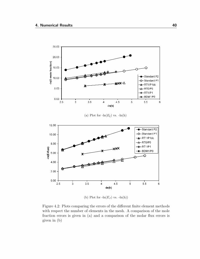
Figure 4.2 shows plots of -ln(E) as a function of -ln(h) for all methods. A linear
best fit was found using the least squares method, so that the slope of the lines could
be used to determine the order of convergence for each method. The L2 errors and
order of convergence for all these methods are summarized in Figure 4.2 and Table
4.1.
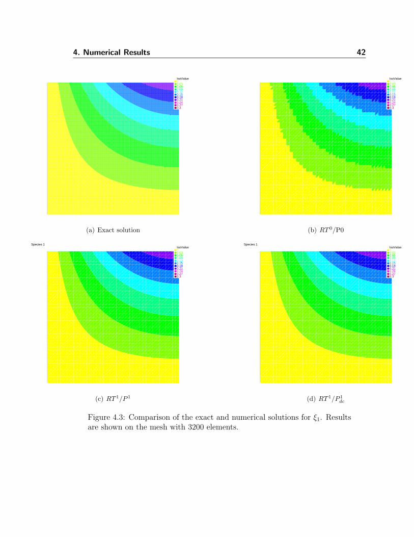
A comparison of the exact functions with some of the mixed finite element ap-
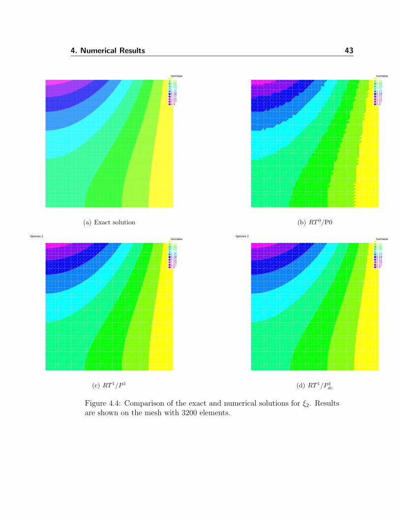
proximations can be seen in Figures 4.3 and 4.4. In all cases, the finite element so-
lutions for the concentrations look very similar to the exact solutions. The RT 0/P 0dc
solution shows small wiggles in the mole fraction isolines due to the piecewise constant
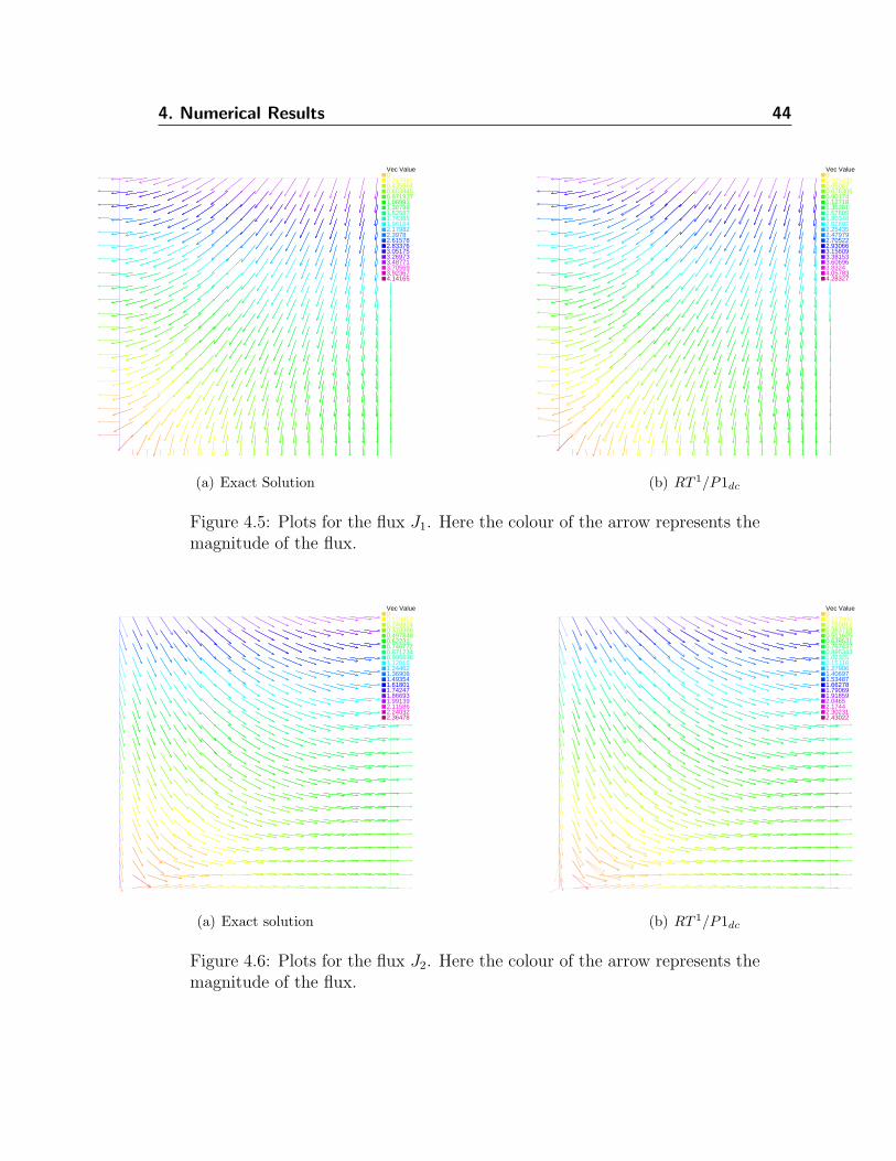
approximation of this variable. On Figures 4.5 and 4.6 , the fluxes computed by the
RT 1/P 1dc mixed finite element method look similar to the exact fluxes. We only show
4. Numerical Results 39
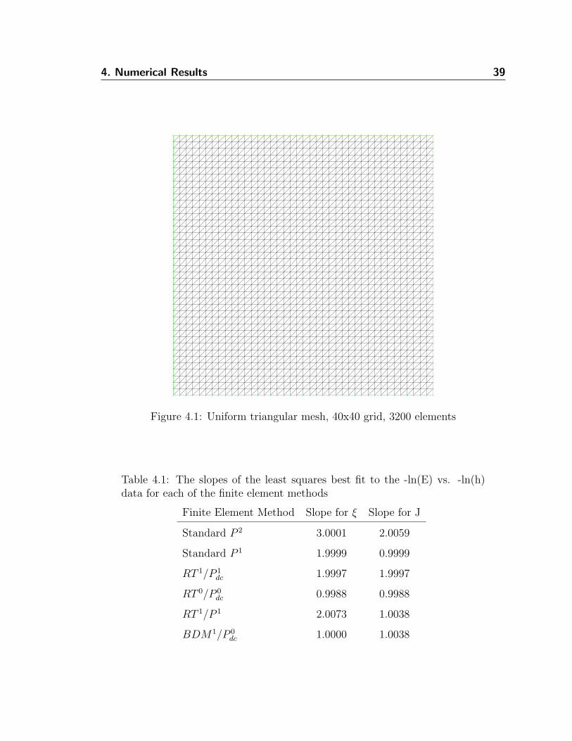
Figure 4.1: Uniform triangular mesh, 40x40 grid, 3200 elements
Table 4.1: The slopes of the least squares best fit to the -ln(E) vs. -ln(h)data for each of the finite element methods
Finite Element Method Slope for ξ Slope for J
Standard P 2 3.0001 2.0059
Standard P 1 1.9999 0.9999
RT 1/P 1dc 1.9997 1.9997
RT 0/P 0dc 0.9988 0.9988
RT 1/P 1 2.0073 1.0038
BDM1/P 0dc 1.0000 1.0038
4. Numerical Results 40
(a) Plot for -ln(Eξ) vs. -ln(h)
(b) Plot for -ln(EJ ) vs. -ln(h))
Figure 4.2: Plots comparing the errors of the different finite element methodswith respect the number of elements in the mesh. A comparison of the molefraction errors is given in (a) and a comparison of the molar flux errors isgiven in (b)
4. Numerical Results 41
the flux calculated using the RT 1/P 1dc method since the other methods yield identical
results.
For RT 0/P 0dc and BDM1/P 0
dc it can be seen that both the mole fractions and
the fluxes have a first order convergence rate. Similarly RT 1/P 1dc has a second order
convergence rate in both variables. The standard P k methods have the same k + 1
order convergence in the concentration variable that the RT k/P kdc method has. How-
ever, when we attempt to recover the flux from the standard finite element solution
we lose an order of accuracy.
4. Numerical Results 42
IsoValue00.030.060.090.120.150.180.210.240.270.3
(a) Exact solution
IsoValue00.030.060.090.120.150.180.210.240.270.3
(b) RT 0/P0
IsoValue00.030.060.090.120.150.180.210.240.270.3
Species 1
(c) RT 1/P 1
IsoValue00.030.060.090.120.150.180.210.240.270.3
Species 1
(d) RT 1/P 1dc
Figure 4.3: Comparison of the exact and numerical solutions for ξ1. Resultsare shown on the mesh with 3200 elements.
4. Numerical Results 43
IsoValue00.030.060.090.120.150.180.210.240.270.3
(a) Exact solution
IsoValue00.030.060.090.120.150.180.210.240.270.3
(b) RT 0/P0
IsoValue00.030.060.090.120.150.180.210.240.270.3
Species 2
(c) RT 1/P 1
IsoValue00.030.060.090.120.150.180.210.240.270.3
Species 2
(d) RT 1/P 1dc
Figure 4.4: Comparison of the exact and numerical solutions for ξ2. Resultsare shown on the mesh with 3200 elements.
4. Numerical Results 44
Vec Value00.2179820.4359640.6539450.8719271.089911.307891.525871.743851.961842.179822.39782.615782.833763.051753.269733.487713.705693.923674.14165
(a) Exact Solution
Vec Value00.2254350.450870.6763050.901741.127181.352611.578051.803482.028922.254352.479792.705222.930663.156093.381533.606963.83244.057834.28327
(b) RT 1/P1dc
Figure 4.5: Plots for the flux J1. Here the colour of the arrow represents themagnitude of the flux.
Vec Value00.1244620.2489240.3733860.4978480.622310.7467720.8712340.9956961.120161.244621.369081.493541.618011.742471.866931.991392.115862.240322.36478
(a) Exact solution
Vec Value00.1279060.2558120.3837180.5116250.6395310.7674370.8953431.023251.151161.279061.406971.534871.662781.790691.918592.04652.17442.302312.43022
(b) RT 1/P1dc
Figure 4.6: Plots for the flux J2. Here the colour of the arrow represents themagnitude of the flux.
4. Numerical Results 45
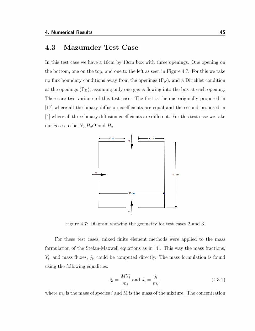
4.3 Mazumder Test Case
In this test case we have a 10cm by 10cm box with three openings. One opening on
the bottom, one on the top, and one to the left as seen in Figure 4.7. For this we take
no flux boundary conditions away from the openings (ΓN), and a Dirichlet condition
at the openings (ΓD), assuming only one gas is flowing into the box at each opening.
There are two variants of this test case. The first is the one originally proposed in
[17] where all the binary diffusion coefficients are equal and the second proposed in
[4] where all three binary diffusion coefficients are different. For this test case we take
our gases to be N2,H2O and H2.
Figure 4.7: Diagram showing the geometry for test cases 2 and 3.
For these test cases, mixed finite element methods were applied to the mass
formulation of the Stefan-Maxwell equations as in [4]. This way the mass fractions,
Yi, and mass fluxes, ji, could be computed directly. The mass formulation is found
using the following equalities:
ξi =MYimi
and Ji =jimi
, (4.3.1)
where mi is the mass of species i and M is the mass of the mixture. The concentration
4. Numerical Results 46
term ctot was also replaced with ρ/M , where ρ is the density of the mixture. The
mass formulation of the Stefan-Maxwell equations is:
−∇MYimi
=M2
ρ
n∑j=1
Yjji − YijjmimjDij
, (4.3.2)
∇ · jimi
= ri, (4.3.3)
n∑i=1
Yi = 1, (4.3.4)
n∑i=1
ji = 0. (4.3.5)
We can proceed to put the mass formulation into a mixed variational formulation
as we did with the mole formulation. When this is done we arrive at the following
bilinear form a(·, ·) for ternary diffusion:
a(j, q) =
∫Ω
M2
ρ
((1
m1m3D13
− Y2α
)j1 + Y1αj2
)· q1 dx (4.3.6)
+
∫Ω
M2
ρ
(Y2βj1 +
(1
m2m3D23
− Y1β
)j2
)· q2 dx, (4.3.7)
where α = 1m1m3D13
− 1m1m2D12
and β = 1m2m3D23
− 1m1m2D12
. For the total mass and
density we have the following:
ρ = Y1m1 + Y2m2 + Y3m3, (4.3.8)
M =1
Y1
m1+ Y2
m2+ Y3
m3
. (4.3.9)
The other parts of the mixed formulation are found just by substituting in 4.3.1.
With this formulation we can now proceed with the next two test cases.
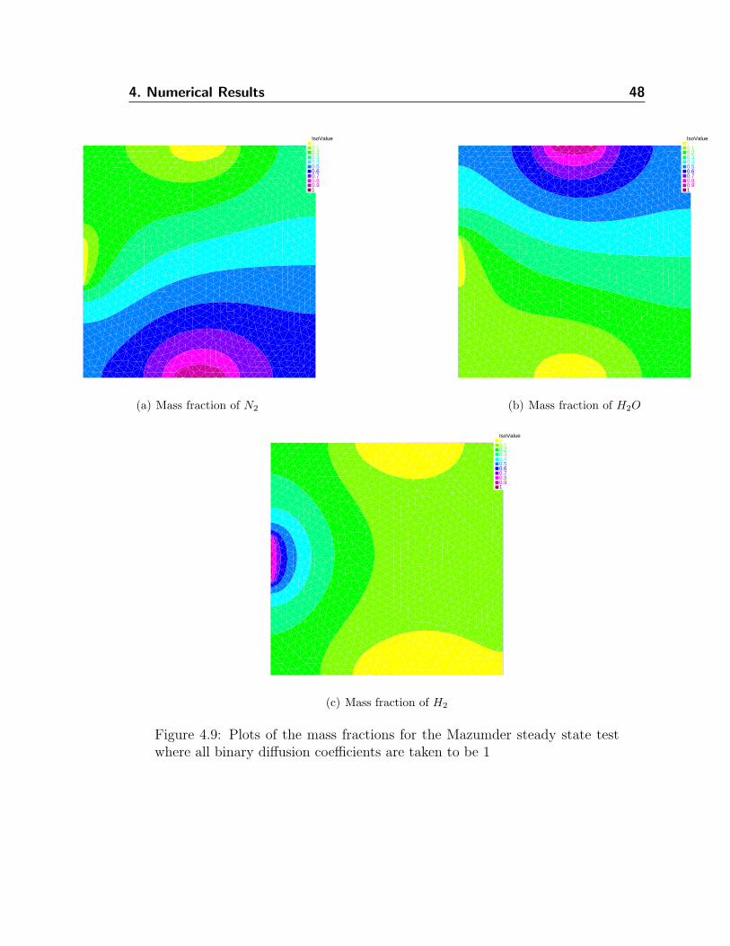
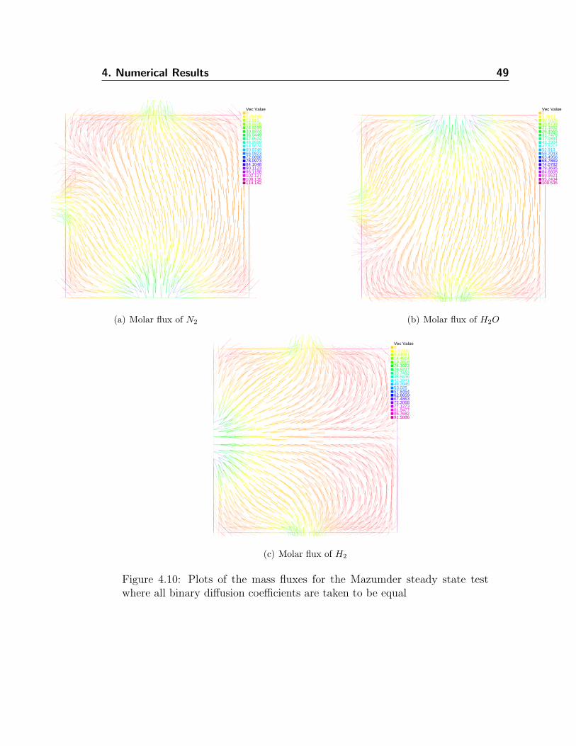
For the Mazumber test case all the binary diffusion coefficients are taken to be
equal to 10 cm2/s. The value of the coefficient will not change the solution for the
mass fractions [4], it will however change the flux. A non-uniform mesh was created
using FreeFEM++’s “buildmesh” function. The mesh can be seen in Figure 4.8.
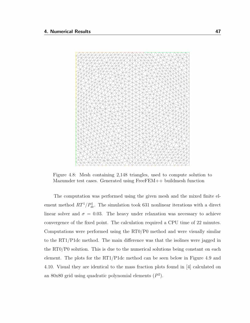
4. Numerical Results 47
Figure 4.8: Mesh containing 2,148 triangles, used to compute solution toMazumder test cases. Generated using FreeFEM++ buildmesh function
The computation was performed using the given mesh and the mixed finite el-
ement method RT 1/P 1dc. The simulation took 631 nonlinear iterations with a direct
linear solver and σ = 0.03. The heavy under relaxation was necessary to achieve
convergence of the fixed point. The calculation required a CPU time of 22 minutes.
Computations were performed using the RT0/P0 method and were visually similar
to the RT1/P1dc method. The main difference was that the isolines were jagged in
the RT0/P0 solution. This is due to the numerical solutions being constant on each
element. The plots for the RT1/P1dc method can be seen below in Figure 4.9 and
4.10. Visual they are identical to the mass fraction plots found in [4] calculated on
an 80x80 grid using quadratic polynomial elements (P 2).
4. Numerical Results 48
IsoValue00.10.20.30.40.50.60.70.80.91
(a) Mass fraction of N2
IsoValue00.10.20.30.40.50.60.70.80.91
(b) Mass fraction of H2O
IsoValue00.10.20.30.40.50.60.70.80.91
(c) Mass fraction of H2
Figure 4.9: Plots of the mass fractions for the Mazumder steady state testwhere all binary diffusion coefficients are taken to be 1
4. Numerical Results 49
Vec Value06.0074912.01518.022524.029930.037436.044942.052448.059954.067460.074966.082372.089878.097384.104890.112396.1198102.127108.135114.142
(a) Molar flux of N2
Vec Value05.291310.582615.873921.165226.456531.747837.039142.330447.621752.91358.204363.495668.786974.078279.369584.660889.952195.2434100.535
(b) Molar flux of H2O
Vec Value04.820459.6409114.461419.281824.102328.922733.743238.563643.384148.204553.02557.845462.665967.486372.306877.127381.947786.768291.5886
(c) Molar flux of H2
Figure 4.10: Plots of the mass fluxes for the Mazumder steady state testwhere all binary diffusion coefficients are taken to be equal
4. Numerical Results 50
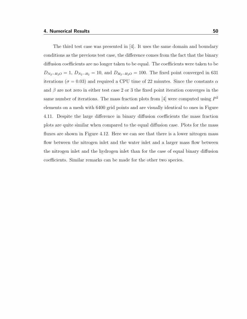
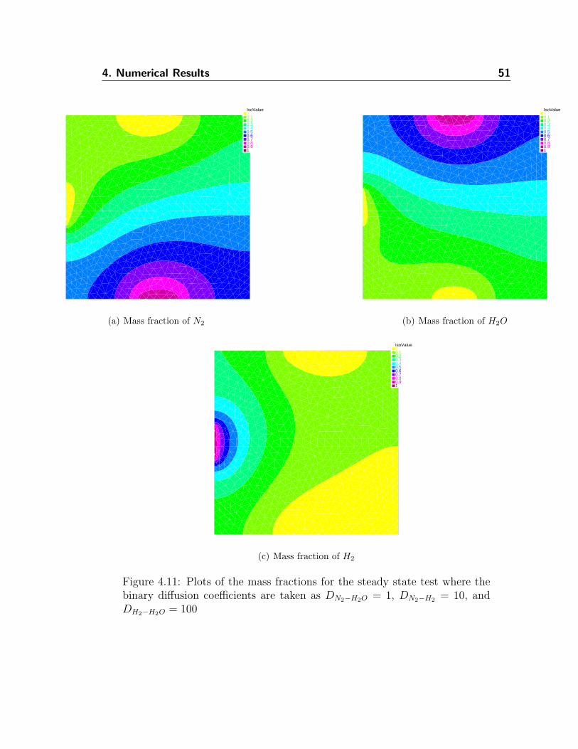
The third test case was presented in [4]. It uses the same domain and boundary
conditions as the previous test case, the difference comes from the fact that the binary
diffusion coefficients are no longer taken to be equal. The coefficients were taken to be
DN2−H2O = 1, DN2−H2 = 10, and DH2−H2O = 100. The fixed point converged in 631
iterations (σ = 0.03) and required a CPU time of 22 minutes. Since the constants α
and β are not zero in either test case 2 or 3 the fixed point iteration converges in the
same number of iterations. The mass fraction plots from [4] were computed using P 2
elements on a mesh with 6400 grid points and are visually identical to ones in Figure
4.11. Despite the large difference in binary diffusion coefficients the mass fraction
plots are quite similar when compared to the equal diffusion case. Plots for the mass
fluxes are shown in Figure 4.12. Here we can see that there is a lower nitrogen mass
flow between the nitrogen inlet and the water inlet and a larger mass flow between
the nitrogen inlet and the hydrogen inlet than for the case of equal binary diffusion
coefficients. Similar remarks can be made for the other two species.
4. Numerical Results 51
IsoValue00.10.20.30.40.50.60.70.80.91
(a) Mass fraction of N2
IsoValue00.10.20.30.40.50.60.70.80.91
(b) Mass fraction of H2O
IsoValue00.10.20.30.40.50.60.70.80.91
(c) Mass fraction of H2
Figure 4.11: Plots of the mass fractions for the steady state test where thebinary diffusion coefficients are taken as DN2−H2O = 1, DN2−H2 = 10, andDH2−H2O = 100
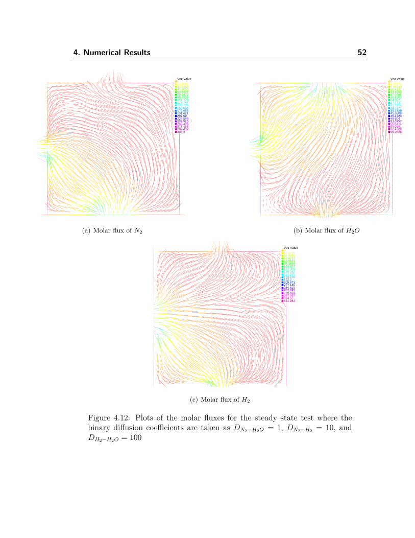
4. Numerical Results 52
Vec Value015.968431.936947.905363.873779.842295.8106111.779127.747143.716159.684175.653191.621207.59223.558239.526255.495271.463287.432303.4
(a) Molar flux of N2
Vec Value03.471716.9434310.415113.886917.358620.830324.30227.773731.245434.717138.188941.660645.132348.60452.075755.547459.019162.490865.9626
(b) Molar flux of H2O
Vec Value017.472834.945552.418369.891187.3639104.837122.309139.782157.255174.728192.2209.673227.146244.619262.092279.564297.037314.51331.983
(c) Molar flux of H2
Figure 4.12: Plots of the molar fluxes for the steady state test where thebinary diffusion coefficients are taken as DN2−H2O = 1, DN2−H2 = 10, andDH2−H2O = 100

Chapter 5
Conclusion
The contributions of the thesis are now summarized and future work is considered.
5.1 Contribution of this Thesis
In this thesis the Stefan-Maxwell equations for the diffusion of n species were con-
sidered in the context of abstract saddle point problems. Such a setting was never
investigated for these equations. A main benefit is the ability to solve for both the
fluxes and the molar fractions without rewriting the Stefan-Maxwell equations. The
difficulty in the application of the mixed finite element theory to the Stefan-Maxwell
equations is the presence of several primal and dual variables, all linked together
through a degenerate system of partial differential equations. To remove this degen-
eracy, we had to express one variable from the others and find a strategy to have a
generic substitution technique that applies to n-ary diffusion. While we could pro-
pose a variational formulation for n-ary diffusion, the analysis of the well-posedness
of the problem stands only in the ternary case, and only after a linearization of the
system. In the case of quaternary diffusion and above, using the Gershgorin circle
theorem to obtain lower bounds on the eigenvalues of the quadratic form becomes
53
5. Conclusion 54
very cumbersome and alternate technique would be recommended.
In chapter 2, a mixed variational formulation was derived for a linearized version
of the n-ary Stefan-Maxwell equations. Then the case of ternary diffusion was ana-
lyzed and shown to be well-posed when the binary diffusion coefficients were within
a certain range of each other. In much of the literature the well-posedness of the
Stefan-Maxwell equations is not considered. While the considerations of chapter 2
were for a linearized version of the Stefan-Maxwell equations, investigation of the
fixed point could extend the work of chapter 2 to conditions for the well-posedness of
the fully nonlinear Stefan-Maxwell equations.
In chapter 3, the linearized mixed variational formulation was discretized using
a mixed finite element approach. Applying standard theory for mixed finite element
methods showed that whenever the linearized Stefan-Maxwell equations were well-
posed, then properly chosen mixed finite element methods converge. An investigation
into the fixed point could also extend the theoretical results of the numerical method
to the nonlinear case.
The method was tested explicitly in chapter 4 on a manufactured problem. Here
the error estimates from chapter 3 were explicitly confirmed through numerical tests.
It was also shown that an order of convergence is lost when calculating the flux using
standard methods. Two other numerical test cases were considered and compared
to other solutions attempted in the literature. A main contribution of this chapter
is that it shows that the mixed finite element method can be used to get species
concentration solutions similar to the literature, while also getting infomation about
species flux. Furthermore, the mesh size needed for solution convergence was smaller
than in previous work.
5. Conclusion 55
5.2 Future Work
Some areas for future work:
1. Expand on the conditions for when the method is well-posed. One of the
tests performed in this paper went way outside the conditions for proven well-
posedness. Additionally, the condition of coerciveness of the bilinear form a(·, ·)
is stronger than necessary, a weaker pair of inf-sup conditions are all that is nec-
essary for well-posedness of the saddle point problem.
2. Investigate the fixed point method used to determine conditions for when it
converges and when it does not.
3. Apply the mixed finite element to more applied engineering problems e.g. in
fuel cells or biology, perhaps involving time dependent phenomena.
Bibliography
[1] N.S. Abdullah and D.B. Das. Modelling nutrient transport in hollow fibre mem-
brane bioreactor for growing bone tissue with consideration of multi-component
interactions. Chemical Engineering Science, 62(21):5821–5839, 2007.
[2] K.E. Atkinson and W. Han. Theoretical Numerical Analysis: A Functional Anal-
ysis Framework. Mathematics and Statistics. Springer-Verlag New York, 2009.
[3] D. Bothe. On the Maxwell-Stefan Approach to Multicomponent Diffusion.
In Joachim Escher, Patrick Guidotti, Matthias Hieber, Piotr Mucha, Jan W.
Pruss, Yoshihiro Shibata, Gieri Simonett, Christoph Walker, and Wojciech Za-
jaczkowski, editors, Parabolic Problems, volume 80 of Progress in Nonlinear Dif-
ferential Equations and Their Applications, pages 81–93. Springer Basel, 2011.
[4] K. Bottcher. Numerical solution of a multi-component species transport prob-
lem combining diffusion and fluid flow as engineering benchmark. International
Journal of Heat and Mass Transfer, 53(2):231–240, 2010.
[5] A. Bressan. Lecture Notes on Sobolev Spaces. http://www.math.psu.edu/
bressan/PSPDF/sobolev-notes.pdf, 2013.
[6] F. Brezzi, J. Douglas, and L.D. Marini. Two families of mixed finite elements for
second order elliptic problems. Numerische Mathematik, 47(2):217–235, 1985.
56
BIBLIOGRAPHY 57
[7] F. Brezzi and M. Fortin. Mixed and hybrid finite elements methods. Springer
series in computational mathematics. Springer-Verlag, 1991.
[8] B. Carnes and G. F. Carey. Local boundary value problems for the error in
FE approximation of non-linear diffusion systems. International Journal for
Numerical Methods in Engineering, 73(5):665–684, 2008.
[9] Y.P. de Diego, F.E. Wubbolts, and P.J. Jansens. Modelling mass transfer in the
PCA process using the Maxwell-Stefan approach. The Journal of Supercritical
Fluids, 37(1):53–62, 2006.
[10] V.V. Dilman. Combined method for studying and calculating the multicom-
ponent diffusion in a mixture with an inert gas. Theoretical Foundations of
Chemical Engineering, 42:166–170, 2008.
[11] J.B. Duncan and H.L. Toor. An experimental study of three component gas
diffusion , 8(1):38–41, 1962. AIChE Journal, 8(1):38–41, 1962.
[12] J. Gopalakrishnan and W. Qiu. Partial expansion of a Lipschitz domain and
some applications. Frontiers of Mathematics in China, 7:249–272, 2012.
[13] F. Hecht. FreeFEM++. http://www.freefem.org/ff++/ftp/freefem++doc.
pdf, 2013.
[14] I. Hsing and P. Futerko. Two-dimensional simulation of water transport in poly-
mer electrolyte fuel cells. Chemical Engineering Science, 55(19):4209–4218, 2000.
[15] R. Krishna and J.A. Wesselingh. The Maxwell-Stefan approach to mass transfer.
Chemical Engineering Science, 52(6):861–911, 1997.
[16] B. Grec L. Boudin and F. Salvarani. A Mathematical and Numerical Analysis
of the Maxwell-Stefan Diffusion Equations. Discrete Contin. Dyn. Syst, Ser. B
17(5)(3):1427–1440, 2012.
BIBLIOGRAPHY 58
[17] S. Mazumder. Critical assessment of the stability and convergence of the
equations of multi-component diffusion. Journal of Computational Physics,
212(1):383–392, 2006.
[18] K.S.C. Peerenboom, J. van Dijk, J.H.M. ten Thije Boonkkamp, L. Liu, W.J.
Goedheer, and J.J.A.M. van der Mullen. Mass conservative finite volume dis-
cretization of the continuity equations in multi-component mixtures. Journal of
Computational Physics, 230(9):3525–3537, 2011.
[19] G. Psofogiannakis, Y. Bourgault, B.E. Conway, and M. Ternan. Mathematical
model for a direct propane phosphoric acid fuel cell. Journal of Applied Electro-
chemistry, 36(1):115–130, 2006.
[20] A. Quarteroni and A. Valli. Numerical Approximation of Partial Differential
Equations. Springer Series in Computational Mathematics. Springer, 2008.
[21] P.A. Raviart and J.M. Thomas. A mixed finite element method for 2-nd order
elliptic problems. In Ilio Galligani and Enrico Magenes, editors, Mathematical
Aspects of Finite Element Methods, volume 606 of Lecture Notes in Mathematics,
pages 292–315. Springer Berlin Heidelberg, 1977.
[22] R. Taylor and R. Krishna. Multicomponent Mass Transfer. Wiley Series in
Chemical Engineering. Wiley, 1993.
[23] R. Temam. Navier-Stokes Equations: Theory and Numerical Analysis. In Navier-
Stokes Equations: Theory and Numerical Analysis, volume 2 of Studies in Math-
ematics and Its Applications, pages iv–. Elsevier, 1976.


![Eigenanalysis of Electromagnetic Structures Based on the ...the aid of numerical techniques and particular the Finite Element Method (FEM), e.g. [1]. Addressing the first steps of](https://static.documents.pub/doc/80x56/5f498cecfb8c3f4f28364fe5/eigenanalysis-of-electromagnetic-structures-based-on-the-the-aid-of-numerical.jpg)
