Mixed Initial-Boundary Value Problems for Scalar Conservation Laws

Mixed Initial-Boundary Value Problems forScalar Conservation Laws: Application to the

Modeling of Transportation Networks

Issam S. Strub and Alexandre M. Bayen

Civil Systems, Department of Civil and Environmental Engineering,University of California, Berkeley, CA, 94720-1710

[email protected] Systems, Department of Civil and Environmental Engineering,

University of California, Berkeley, CA, [email protected]

Tel.: (510)-642-2468; Fax:(510)-643-5264

Abstract. This article proves the existence and uniqueness of a weaksolution to a scalar conservation law on a bounded domain. A weak for-mulation of hybrid boundary conditions is needed for the problem to bewell posed. The boundary conditions are represented by a hybrid au-tomaton with switches between the modes determined by the directionof characteristics of the system at the boundary. The existence of thesolution results from the convergence of a Godunov scheme derived inthis article. This weak formulation is written explicitly in the context ofa strictly concave flux function (relevant for highway traffic). The nu-merical scheme is then applied to a highway scenario with data from theI210 highway obtained from the California PeMS system. Finally, the ex-istence of a minimizer of travel time is obtained, with the correspondingoptimal boundary control.

Keywords: Weak solution of scalar conservation laws, Weak hybridboundary conditions, LWR PDE, Highway traffic modeling, Boundarycontrol.

1 Introduction

This article is motivated by recent research efforts which investigate the problemof controlling highway networks with metering strategies that can be appliedat the on-ramps of the highway (see in particular [46] and references therein).The seminal models of highway traffic go back to the 1950’s with the workof Lighthill-Whitham [36] and Richards [43] who tried to use fluid dynamicsequations to model traffic flow. The resulting theory, called Lighthill-Whitham-Richards (LWR) theory relies on a scalar hyperbolic conservation law, with aconcave flux function. Very few approaches have tackled the problem of boundarycontrol of scalar conservation laws in bounded domains in an explicit mannerdirectly applicable for engineering. Unlike the viscous Burgers equation, whichhas been is focus of numerous ongoing studies, very few results exist for the

J Hespanha and A. Tiwari (Eds.): HSCC 2006, LNCS 3927, pp. 552–567, 2006.c© Springer-Verlag Berlin Heidelberg 2006.

Mixed Initial-Boundary Value Problems for Scalar Conservation Laws 553

inviscid Burgers equation, which is traditionally used as a model problem forhyperbolic conservation laws. Differential flatness [42] and Lyapunov theory [30]have been explored and appear as promising directions to investigate.

The proper notion of weak solution for the LWR partial differential equation(PDE), called entropy solution was first defined by Oleinik [39] in 1957. Eventhough this work was known to the traffic community, it does not (as far as weknow) appear explicitly in the transportation literature before the 1990’s withthe work of Ansorge [4]. The entropy solution has been since acknowledged asthe proper weak solution to the LWR PDE [18] for traffic models. Unfortunatelythe work of Oleinik in its initial form [39] does not hold for bounded domains,i.e. it would only work for infinitely long highways with no on-ramps or off-ramps. Bounded domains, i.e. highways of finite length (required to model onand off-ramps) imply the use of boundary conditions, for which the existenceand uniqueness of a weak solution is not straightforward.

The first result of existence and uniqueness of a weak solution of the LWRPDE in the presence of boundary conditions follows from the work of Bardos,Leroux and Nedelec [8], in the more general context of a first order quasilinearPDE on a bounded open set of R

n. In particular, they introduce a weak formu-lation of the boundary conditions for which the initial-boundary value problemis well-posed.

We begin this article by explaining that in general, one cannot expect theboundary conditions to be fulfilled pointwise a.e. and we provide several exam-ples to illustrate this fact. We then turn to the specific case of highway trafficflow, for which we are able to state a simplified weak hybrid formulation of theboundary conditions, and prove the existence and uniqueness of a weak solutionto the LWR PDE, the former resulting from the convergence of the associatedGodunov scheme to the entropy solution of the PDE. This represents a majorimprovement from the existing traffic engineering literature, where boundaryconditions are expected to be fulfilled pointwise and therefore existence of asolution and convergence of the numerical schemes to this solution are not guar-anteed. We illustrate the applicability of the method and the numerical schemedeveloped in this work with a highway scenario, using data for the I210 high-way, obtained from the California PeMS system. In particular, we show that themodel is able to reproduce flow variations on the highway with a good accuracyover a period of five hours. The last part of the article is devoted to the boundarycontrol of the LWR PDE and its application to a highway optimization problem,in which boundary control is used to minimize travel time on a given stretch ofthe highway.

2 The Need for a Weak Formulation of Hybrid BoundaryConditions

This section shows three examples of the sort of trouble one runs into whenprescribing the boundary conditions in the strong sense. Numerous articles solvea discrete version of this type of problems. Regardless of the numerical schemes

554 I.S. Strub and A.M. Bayen

used (Godunov [22], Jameson-Schmidt-Turkel [25, 26], Daganzo [17, 18]), thesemethods suffer from the same difficulties: the authors solve a discrete problemwith strong boundary conditions which entails that the corresponding continuousproblem is usually ill-posed, i.e. does not have a solution. While the numericalschemes listed above might still yield a numerical output, this numerical datawould be meaningless since the initial boundary-value problem does not have asolution in the first place. The object of this work is not to make an endless listof engineering articles which exhibit such shortcomings: we will just mention aprevious paper from one of the authors [9] and let the reader discover that thisis far from being an exception... To sum up, boundary conditions may only beprescribed on the part of the boundary where the characteristics are incoming,that is entering the domain.

Example 1: Advection equation. We start by considering the simple examplewhere the propagation speed is a constant c,

∂ρ

∂t+ c

∂ρ

∂x= 0 for (x, t) ∈ (a, b) × (0, T ).

In that case, one can clearly see that the boundary condition is either prescribedon the left (x = a) if the speed c is positive or the right (x = b) if the speed isnegative. While finding the sign of the speed is quite simple in the linear case,it becomes more subtle when dealing with a nonlinear conservation law such asthe LWR PDE as this sign is no longer constant.

Example 2: LWR PDE, shock wave back-propagation due to a bottleneck. For thisexample, we consider the LWR PDE with a Greenshields flux function [24]:

∂ρ

∂t+ v

(1 − 2ρ

ρ∗

)∂ρ

∂x= 0 (1)

where ρ = ρ(x, t) is the vehicle density on the highway, ρ∗ is the jam density andv is the free flow density (see [17, 18] for more explanations on the interpretationof these parameters). We consider a road of length L = 30, ρ∗ = 4 and v = 1(dummy values), and an initial density profile given by ρ0(x) � ρ(x, 0) = 2 ifx ∈ [0, 10], ρ0(x) � ρ(x, 0) = 4 if x ∈ (10, 20], ρ0(x) � ρ(x, 0) = 1 if x > 20. Thehighway might be bounded or unbounded on the right at x = L = 30 (it does notmatter for our problem). We assume free flow conditions at x = L, that we cancontrol the inflow at x = 0, and we try to prescribe it pointwise, i.e. ρ(0, t) = 2for all t (this corresponds to sending the maximum flow onto the highway). Thesolution to this problem can easily be computed by hand (for example by themethod of characteristics, see Figure 1, left). The solution to this problem reads��

ρ(x, t) = 2 if t ≤ 2(10 − x) AC: shockρ(x, t) = 4 if 2(10 − x) ≤ t ≤ 20 − x BC: left edge of exp. waveρ(x, t) = 2(1 − (x − 20)/t) if t ≥ max{20 − x, 2(x − 20)} CBD is an expansion waveρ(x, t) = 1 if t ≤ 2(x − 20) BD: right edge of exp.wave

As can be seen, limx→0+ ρ(x, t) = 2 for t ≤ 20 and limx→0+ ρ(x, t) = 2(1 + 20/t)for t > 20. Thus, the boundary condition ρ(0, t) = 2 is no longer verified as soon


Fig. 1. Left: Characteristics for the solution of the LWR PDE for Example 2. Right:corresponding value of the solution at successive times. The arrow represents the valueof the input at x = 0, which becomes irrelevant for t ≥ 20.

as t ≥ 20. This phenomenon is crucial in traffic flow models: it represents theback-propagation of congestion (i.e. upstream). If the location x = 0 was the endof a link merging into the highway (that we could potentially control), the casewhen ρ(0+, t) > ρ∗ is congested would correspond to a situation in which theupstream flow (x = 0−) is imposed by the downstream flow (x = 0+), i.e. theboundary condition on the left becomes irrelevant. When ρ(0+, t) < ρ∗ is notcongested, the boundary condition is relevant and can be imposed pointwise.

Example 3: Burgers equation. We now consider the inviscid Burgers equation on(0, 1) × (0, T ). If we try to prescribe strong boundary conditions at both ends,the problem becomes ill-posed. Burgers equation reads:

∂u

∂t+ u

∂u

∂x= 0 (2)

The initial value is u(x, 0) = 1, and the boundary conditions u(0, t) = u(1, t) = 0on [0, 1]. The solution of (2) with these boundary conditions is for t < 1 :{

u(x, t) = xt if x < t self similar expansion wave

u(x, t) = 1 if x > t convection to the right with speed 1

We notice that the boundary condition is not satisfied at x = 1. Since the datapropagates at speed u, they are leaving [0, 1] at x = 1 while they stay in [0, 1] asa rarefaction wave at x = 0.

3 Traffic Flow Equation with Hybrid BoundaryConditions

We consider a mixed initial-boundary value problem for a scalar conservationlaw on (a, b) × (0, T ).

∂ρ

∂t+

∂q(ρ)∂x

= 0 (3)

with the initial condition


ρ(x, 0) = ρ0(x) on (a, b)

and the boundary conditions

ρ(a, t) = ρa(t) and ρ(b, t) = ρb(t) on (0, T ).

As usual with nonlinear conservation laws, in general there are no smooth solu-tions to this equation and we have to consider weak solutions (see for example[10], [19], [45]). In this article we use the space BV of functions of bounded vari-ation which appears very often when dealing with conservation laws. A functionof bounded variation is a function in L1 such that its weak derivative is uniformlybounded. We refer the intrigued readers to the book from Ambrosio, Fusco andPallara [1] for many more properties and applications of BV functions. Othervaluable references on BV functions include the article by Vol’pert [48] and thebook from Evans and Gariepy [20].

In our problem, we make the assumption that the flux q is continuous andthat the initial and boundary conditions ρ0, ρa, ρb are functions of boundedvariation. When the flux q models the flux of cars in terms of the car densityρ we obtain the LWR PDE. As explained earlier on, boundary conditions maynot be fulfilled pointwise a.e., thus following [8], we shall require that an entropysolution of (3) satisfy a weak formulation of the boundary conditions:

L(ρ(a, t), ρa(t)) = 0 and R(ρ(b, t), ρb(t)) = 0

whereL(x, y) = sup

k∈I(x,y)(sg(x − y)(q(x) − q(k)) and

R(x, y) = infk∈I(x,y)

(sg(x − y)(q(x) − q(k)) for x, y ∈ R

and I(x, y) = [inf(x, y), sup(x, y)] with sg denoting the sign function. In thecase of a strictly concave flux (such as the Greenshields [24] and Greenberg [23]models used in traffic flow modeling), the boundary conditions can be writtenas (Le Floch gives analogous conditions in the case of a strictly convex flux in[33]): ⎧⎪⎨

⎪⎩ρ(a, t) = ρa(t) orq′(ρ(a, t)) � 0 and q′(ρa(t)) � 0 orq′(ρ(a, t)) � 0 and q′(ρa(t)) � 0 and q(ρ(a, t)) � q(ρa(t))

(4)

Similarly, the boundary condition at b is:⎧⎪⎨⎪⎩

ρ(b, t) = ρb(t) orq′(ρ(b, t)) � 0 and q′(ρb(t)) � 0 orq′(ρ(b, t)) � 0 and q′(ρb(t)) � 0 and q(ρ(b, t)) � q(ρb(t))

(5)

As noticed in [33], we can always assume the boundary data are entering thedomain at both ends. Indeed, if for example q′(ρa(t)) < 0 on a subset I of R+of positive measure, the boundary data:


ρa(t) =

{q′−1(0) if t ∈ I

ρa(t) otherwise(6)

will yield the same solution. With this assumption the boundary conditions canbe written as:

{ρ(a, t) = ρa(t) orq′(ρ(a, t)) � 0 and q(ρ(a, t)) � q(ρa(t))

(7)

and {ρ(b, t) = ρb(t) orq′(ρ(b, t)) � 0 and q(ρ(b, t)) � q(ρb(t))

(8)

We can now define an notion of entropy solution for a scalar conservation law(3) with initial and boundary conditions.

Interpretation of the hybrid automaton for concave flux functions. Figure 2(left) shows the three-mode automaton corresponding to (4). The first mode,ρ(a, t) = ρa(t) corresponds to the situation in which the boundary conditionρa(t) is effectively applied (as in the strong sense). The second mode q′(ρ(a, t)) �0 and q′(ρa(t)) � 0 corresponds to a situation in which the characteristics exitthe domain at x = a for both the solution ρ(a, t) and the prescribed boundarycondition ρa(t) (therefore the boundary condition does not ‘affect’ the solution).The third mode corresponds to a supercritical ρ(a, t), i.e. ρ(a, t) ≥ ρc (see Fig-ure 3 and [17, 18]), a subcritical ρa(t), i.e. i.e. ρa(t) ≤ ρc, and a prescribed inflowq(ρa(t)) greater than the actual flow q(ρ(a, t)) at x = a. This corresponds to ashock moving to the left (to see this, plug the previous quantities in the Rankine-Hugoniot conditions), which means that the prescribed boundary condition does

Fig. 2. Left: Hybrid automaton encoding the boundary conditions at x = a, corre-sponding to (4). A similar automaton can be constructed for (5). Right: Simplificationof the automaton corresponding to the transformation of (4) into (7). A similar au-tomaton can be constructed for (8) from (5).


not ‘affect’ the solution. The guards for this hybrid systems are thus determinedby the sign of the flux derivative q′(·) and the values of the flux q(·) at x = a.

Definition: A solution of the mixed initial-boundary value problem for the PDE(3) is a function ρ ∈ L∞((a, b)×(0, T )) such that for every k ∈ R, ϕ ∈ C1

c ((0, T )),the space of C1 functions with compact support, and ψ ∈ C1

c ((a, b)×(0, T )) withϕ and ψ nonnegative:

∫ b

a

∫ T

0(|ρ − k|∂ψ

∂t+ sg(ρ − k)(q(ρ) − q(k))

∂ψ

∂x)dxdt � 0

and there exist E0, EL, ER three sets of measure zero such that :

limt→0,t/∈E0

∫ b

a

|ρ(x, t) − ρ0(x)|dx = 0

limx→a,x/∈EL

∫ T

0L(ρ(x, t), ρa(t))ϕ(t)dt = 0

limx→b,x/∈ER

∫ T

0R(ρ(x, t), ρb(t))ϕ(t)dt = 0

With this definition, we now establish the uniqueness by proving anL1- semigroup property following the method introduced by Kruzkov [31] (seealso the articles from Keyfitz [28] and Schonbek [44]).

Let ρ, σ be two solutions of (3), ϕ and ψ two test functions in C1c ((0, T )) and

C1c ((a, b)) respectively and nonnegative; the aforementioned definition yields:

b

a

T

0(|ρ(x, t)−σ(x, t)|ψ(x)ϕ′(t)+sg(ρ(x, t)−σ(x, t))(q(ρ(x, t))−q(σ(x, t)))ϕ(t)ψ′(x)))dxdt � 0

For ψ approximating χ |[a,b], the characteristic function of the interval [a, b], wehave:

� b

a

� T

0|ρ(x, t)−σ(x, t)|ϕ′(t)dt� lim inf

x→b

� T

0sg(ρ(x, t)−σ(x, t))(q(ρ(x, t)−q(σ(x, t)))ϕ(t)dt

− lim supx→a

� T

0sg(ρ(x, t) − σ(x, t))(q(ρ(x, t)) − q(σ(x, t)))ϕ(t)dt.

For a fixed x /∈ EL and t ∈ (0, T ), we can always define k(x, t) ∈ I(σ(x, t), ρa(t))∩I(ρ(x, t), ρa(t)) such that:

sg(ρ(x, t)−σ(x, t))(q(ρ(x, t))−q(σ(x, t))) = sg(ρ(x, t)−ρa(t))(q(ρ(x, t))−q(k(x, t)))

+sg(σ(x, t)−ρa(t))(q(σ(x, t))−q(k(x, t))) � L(ρ(x, t), ρa(x, t))+L(σ(x, t), ρa(x, t)).

The situation is similar in a neighborhood of b which eventually yields:∫ b

a

∫ T

0|ρ(x, t) − σ(x, t)|ϕ′(t)dtdx � 0.


Therefore, for 0 < t0 < t1 < T ,∫ b

a

|ρ(x, t1) − σ(x, t1)|dx �∫ b

a

|ρ(x, t0) − σ(x, t0)|dx

which proves the L1-semigroup property from which the uniqueness follows.

4 Numerical Methods for the Initial-Boundary ValueProblem

In this section, we prove the existence of a solution to equation (3) through theconvergence of the Godunov scheme. Let h = b−a

M and Ii = [a + h(i − 12 ), a +

h(i + 12 )) for i ∈ {0, ..., M}. For r > 0, let Jn = [(n − 1

2 )rh, (n + 12 )rh) with

n ∈ {0, 1, ..., N = E(1 + Trh )}. We approximate the solution ρ by ρn

i on each cellIi ×Jn, with ρh the resulting function on [a, b]× [0, T ]. The initial and boundaryconditions can be written as:{

ρ0i = 1

h

∫Ii

ρ0(x)dx , 0 � i � M

ρn0 = 1

rh

∫Jn

ρa(t)dt and ρnM = 1

rh

∫Jn

ρb(t)dt , 0 � n � N

According to the Godunov scheme [22], ρn+1i is computed from ρn

i by thefollowing algorithm:{

ρni+ 1

2is an element k of I(ρn

i , ρni+1) such that sg(ρn

i+1 − ρni )q(k) is minimal

ρn+1i = ρn

i − r(q(ρni+ 1

2) − q(ρn

i− 12))

Let M0 = max(‖ρ0‖∞, ‖ρa‖∞, ‖ρb‖∞); if the CFL (Courant-Friedrichs-Lewy)condition ([35])

r sup|k|<M0

|q′(k)| � 1

is verified, ρh converges in L1((a, b)×(0, T )) to a solution ρ ∈ BV ((a, b)×(0, T )).The CFL condition yields the following estimates:

|ρn+1i | � (1 + C0h) sup(|ρn

i− 12|, |ρn

i |, |ρni+ 1

2|) + C1h for every i ∈ Z

∑1�i�M

|ρn+1i+1 − ρn+1

i | � (1 + C2h)∑

|i|�M+1

|ρni+1 − ρn

i | + C3Mh2 for every M ∈ N

∑|i|�M

|ρn+1i − ρn

i | �∑

|i|�M+1

|ρni+1 − ρn

i | + C4Mh(1 + supi∈Z

|ρni |) for every M ∈ N

from which we can deduce that a subsequence ρhn converges strongly to a func-

tion ρ ∈ L∞((a, b)× (0, T )) of bounded variation and verifying the initial condi-tion. We also have for k of I(ρn

i , ρni+1)

|ρn+1i −k| � |ρn

i −k|−r(sg(ρni+ 1

2−k)(q(ρn

i+ 12)−q(k))−sg(ρn

i− 12−k)(q(ρn

i− 12)−q(k)))


which shows that ρ is a weak solution of (3). If ϕn = 1rh

∫In

ϕ(t)dt for ϕ ∈C1

c ((0, T )), non negative, we have:�0�n�N

sg(ρni+ 1

2− k)(q(ρn

i+ 12) − q(k))ϕnrh �

�0�n�N

sg(ρn12

− k)(q(ρn12) − q(k))ϕnrh+

+ih‖ϕ′‖∞T (M0 + |k|).Let λ(t) be the weak * limit in L∞((0, T )) of a subsequence of q(ρi

12); the

following inequality holds:� T

0sg(ρ(x, t) − k)(q(ρ(x, t)) − q(k))ϕ(t)dt �

� T

0sg(ρa(t) − k)(λ(t) − q(k))ϕ(t)dt+

+|x − a|‖ϕ′‖∞T (M0 + |k|),

using that sg(ρn12

− k)(q(ρ 12) − q(k)) � sg(ρn

0 − k)(q(ρ 12) − q(k)).

ρ(x, .) is of bounded variation, therefore it converges strongly in L1 sense toa limit α ∈ L∞((0, T )) and it verifies:

sg(α(t) − k)(q(α(t)) − q(k)) � sg(ρa(t) − k)(λ(t) − q(k))

for every k ∈ R and a.e. t ∈ (0, T ). This inequality shows that λ = q(α) a.e.and L(α(t), ρa(t)) � 0 and ρ verifies the weak boundary condition at x = a.Similarly, ρ verifies the corresponding condition at x = b and the existence isproved.

5 Implementation and Simulations for I201W

We now turn to the practical implementation of the Godunov scheme for theLWR PDE. The scheme is written as follows:

ρn+1i = ρn

i − r(qG(ρni , ρn

i+1) − qG(ρni−1, ρ

ni ))

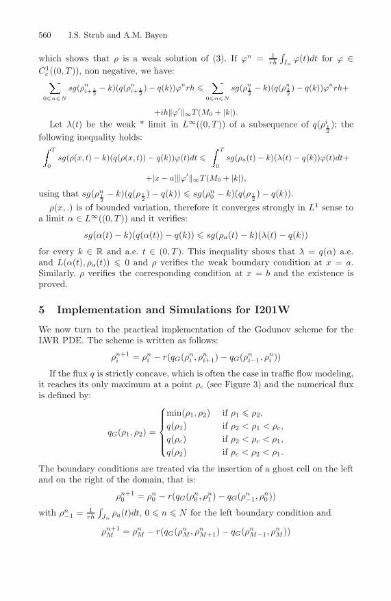
If the flux q is strictly concave, which is often the case in traffic flow modeling,it reaches its only maximum at a point ρc (see Figure 3) and the numerical fluxis defined by:

qG(ρ1, ρ2) =

⎧⎪⎪⎪⎨⎪⎪⎪⎩

min(ρ1, ρ2) if ρ1 � ρ2,

q(ρ1) if ρ2 < ρ1 < ρc,

q(ρc) if ρ2 < ρc < ρ1,

q(ρ2) if ρc < ρ2 < ρ1.

The boundary conditions are treated via the insertion of a ghost cell on the leftand on the right of the domain, that is:

ρn+10 = ρn

0 − r(qG(ρn0 , ρn

1 ) − qG(ρn−1, ρ

n0 ))

with ρn−1 = 1rh

∫Jn

ρa(t)dt, 0 � n � N for the left boundary condition and

ρn+1M = ρn

M − r(qG(ρnM , ρn

M+1) − qG(ρnM−1, ρ

nM ))


Fig. 3. Left: Illustration of the empirical data obtained from the PeMS system. Thehorizontal axis represents the normalized density ρ (i.e. occupancy, see [41, 38] for moredetails). The vertical axis represents the flux q(·). Each track corresponds to a loopdetector measurement. This data can easily be modelled with a strictly concave fluxfunction (solid fit), for which we display the critical density ρc and the jam density, ρ∗.Right: Location of the loop detectors used for measurement and validation purposes.

with ρnM+1 = 1

rh

∫Jn

ρb(t)dt, 0 � n � N on the right of the domain. We illustratean application of this Godunov scheme to the simulation of highway traffic. Acomparison of the density obtained numerically with the corresponding experi-mental density measured by the loop detectors is performed. We consider I210West in Los Angeles and focus on a stretch going from the Santa Anita on-ramp1 to the Baldwin on-ramp 2 in free-flow conditions between midnight and 05:00a.m. The data measured by the loop detectors is accessible through the PeMSsystem (Performance Measurement System [41]); in our case the two detectorsID are 764669 and 717664.

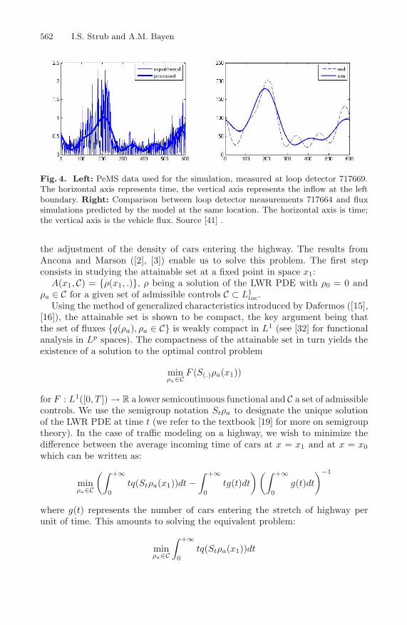
We measure the flow at the loop detector 764669 (left subfigure in Figure 4).The need for signal processing is quite visible; for this example, it was done usingFast Fourier Transform methods. Noise levels are a very important issue withPeMS measurements, that has been covered extensively in the literature and isout of the scope of this work. The comparison with the actual measurementsis performed at the next downstream loop detector (detector 717664), see rightsubfigure in Figure 4. The results shown in this figure illustrate the fact that themethod is able to reproduce traffic flow patterns over an extended period of time(5 hours in the present case). The numerical simulation was done with Fortran

codes from the Clawpack software developed by LeVeque and available at [12],implemented on a Sun Blade workstation. Further model refinements would beneeded to obtain an enhanced matching of the two curves. This is also out ofthe scope of this article (the reader is referred to [38] for more on this topic).

6 Optimization of Travel Time Via Boundary Control

Our next endeavor is directed towards the minimization of the mean time spentby cars traveling through a stretch of highway between x = x0 and x = x1 via


Fig. 4. Left: PeMS data used for the simulation, measured at loop detector 717669.The horizontal axis represents time, the vertical axis represents the inflow at the leftboundary. Right: Comparison between loop detector measurements 717664 and fluxsimulations predicted by the model at the same location. The horizontal axis is time;the vertical axis is the vehicle flux. Source [41] .

the adjustment of the density of cars entering the highway. The results fromAncona and Marson ([2], [3]) enable us to solve this problem. The first stepconsists in studying the attainable set at a fixed point in space x1:

A(x1, C) = {ρ(x1, .)}, ρ being a solution of the LWR PDE with ρ0 = 0 andρa ∈ C for a given set of admissible controls C ⊂ L1

loc.Using the method of generalized characteristics introduced by Dafermos ([15],

[16]), the attainable set is shown to be compact, the key argument being thatthe set of fluxes {q(ρa), ρa ∈ C} is weakly compact in L1 (see [32] for functionalanalysis in Lp spaces). The compactness of the attainable set in turn yields theexistence of a solution to the optimal control problem

minρa∈C

F (S(.)ρa(x1))

for F : L1([0, T ]) → R a lower semicontinuous functional and C a set of admissiblecontrols. We use the semigroup notation Stρa to designate the unique solutionof the LWR PDE at time t (we refer to the textbook [19] for more on semigrouptheory). In the case of traffic modeling on a highway, we wish to minimize thedifference between the average incoming time of cars at x = x1 and at x = x0which can be written as:

minρa∈C

(∫ +∞

0tq(Stρa(x1))dt −

∫ +∞

0tg(t)dt

) (∫ +∞

0g(t)dt

)−1

where g(t) represents the number of cars entering the stretch of highway perunit of time. This amounts to solving the equivalent problem:

minρa∈C

∫ +∞

0tq(Stρa(x1))dt


For this particular problem, we make the following additional assumptions:

– the net flux of cars entering the highway is equal to the total number of carsarriving at the entry: ∫ +∞

0q(ρa(s))ds =

∫ +∞

0g(s)ds

– for every time t > 0 the total number of cars which have entered the highwayis smaller than or equal to the total number of cars that have arrived at theentry from time 0 to t: ∫ t

0q(ρa(s))ds �

∫ t

0g(s)ds

– the number of cars entering the highway is at most equal to the maximumdensity of cars on the highway:

ρa(t) ∈ [0, ρm]

– after a given time T no cars enter the highway:

ρa(t) = 0 for t > T.

The map F : ρ →∫ T

0 q(ρ(t))dt is obviously a continuous functional on L1loc

([0, T ]), hence the existence of a solution of an optimal control ρa.Furthermore, a comparison principle for solutions of scalar nonlinear con-

servation laws with boundary conditions established by Terracina in [47] willallow us to find an explicit expression of the optimal control. Indeed if ρ(x, t)is a weak solution of the LWR PDE, u(x, t) = −

∫ +∞x ρ(y, t)dy is the viscosity

solution ([14]) of the Hamilton-Jacobi equation

∂u

∂t+ q(

∂u

∂x) = q(0).

Since viscosity solutions verify a comparison property [13], so will the solutionof the LWR PDE.

Since∫ T

0 tq(Stρa(x1))dt = T∫ T

0 q(Stρa(x1))dt −∫ T

0

∫ t

0 q(Ssρa(x1))dsdt, theboundary control problem can be rewritten as:

maxρa∈C

∫ T

0

∫ t

0q(Ssρa(x1))dsdt.

As we can assume that the boundary data is always incoming, the comparisonprinciple shows that the optimal control ρ should verify:∫ t

0q(ρ(s))ds �

∫ t

0q(ρa(s))ds, for every t > 0 and ρa ∈ C.

Eventually we obtain the following expression of the optimal control ρ:

ρ(t)=

{q−1(ρm) if g(t) � q(ρm) and

∫ t

0 q(ρ(s))ds <∫ t

0 g(s)ds or g(t) > q(ρm)q−1(g(t)) if g(t) � q(ρm) and

∫ t

0 q(ρ(s))ds =∫ t

0 g(s)ds


7 Conclusion

We have proved the existence and uniqueness of a weak solution to a scalarconservation law on a bounded domain. The proof relies on the weak formu-lation of the hybrid boundary conditions which is necessary for the problemto be well posed. For strictly concave flux functions, the simplified expressionof the weak formulation of the hybrid boundary conditions was written ex-plicitly. The corresponding Godunov scheme was developed and applied on ahighway traffic flow application, using PeMS data for the I210W highway inPasadena. The numerical scheme and the parameters identified for this highwaywere validated experimentally against measured data. Finally, the existence ofa minimizer of travel time was obtained, with corresponding optimal boundarycontrol.

The hybridness of the boundary conditions is closely linked to the one-dimensional nature of the problem (i.e. to the direction of the characteristicsand the corresponding values of the fluxes). The switches between the modes oc-cur based on the value of the solution, which itself acts as a guard. The boundaryconditions derived in this article should thus be viewed as an instantiation ofthe more general weak boundary conditions given in [8], for which a clear hybridstructure appears in the one dimensional case, through a modal behavior.

This article should be viewed as a first step towards building sound meteringcontrol strategies for highway networks: it defines the mathematical solution,and appropriate hybrid boundary conditions to apply in order to pose and solvethe optimal control problem properly. Not using the framework developed herewhile computing numerical solutions of the LWR PDE would lead to ill-posedproblems and therefore the data obtained through a numerical scheme would bemeaningless.

Our result is crucial for highway performance optimization, since by nature, inmost highways, traffic flow control is achieved by on-ramp metering, i.e. bound-ary control. However, results are still lacking in order to generalize our approachto a real highway network. For such a network, PDEs are coupled through bound-ary conditions, which makes the problem harder to pose. Furthermore, optimiza-tion problems arising in transportation networks often cannot be solved as theproblem derived in the last section of this article. In fact, several approacheshave to rely on the computation of the gradient of the optimization functional,which for example could be achieved using adjoint-based techniques. Obtainingthe proper formulation of the adjoint problem, and the corresponding proofsof existence and uniqueness of the resulting solutions represents a challenge forwhich the present result is a building block.

Acknowledgements. We are grateful to Antoine Bonnet and Remy Nolletfor their help with the PeMS data. We acknowledge fruitful discussions withProfessor Roberto Horowitz on highway traffic control problems. I. Strub wishesto thank Professor F. Rezakhanlou for his helpful remarks and bibliographicalreferences.


References

1. L. Ambrosio, N. Fusco, D. Pallara. Functions of bounded variation and freediscontinuity problems. Oxford Mathematical Monographs. The Clarendon Press,Oxford University Press, New York, 2000.

2. F. Ancona, A. Marson. On the attainable set for scalar nonlinear conservationlaws with boundary control. SIAM J. Control Optim., 36(1):290–312, 1998.

3. F. Ancona, A. Marson. Scalar non-linear conservation laws with integrableboundary data. Nonlinear Analysis, 35:687–710, 1999.

4. R. Ansorge. What does the entropy condition mean in traffic flow theory? Trans-portation Research, 24B(2):133–143, 1990.

5. J. A. Atwell, J. T. Borggaard, B. B. King. Reduced order controllers for Burg-ers’ equation with a nonlinear observer. Applied Mathematics and ComputationalScience, 11(6):1311–1330, 2001.

6. J. Baker, A. Armaou, P. D. Christofides. Nonlinear control of incompress-ible fluid flow: Application to burgers’ equation and 2d channel flow. Journal ofMathematical Analysis and Applications, 252:230–255, 2000.

7. A. Balogh, M. Krstic. Burgers’ equation with nonlinear boundary feedback: H1

stability, well posedness, and simulation. Mathematical Problems in Engineering,6:189–200, 2000.

8. C. Bardos, A. Y. Leroux, J. C. Nedelec. First order quasilinear equations withboundary conditions. Comm. Part. Diff. Eqns, 4(9):1017–1034, 1979.

9. A. M. Bayen, R. L. Raffard, C. J. Tomlin. Network congestion alleviation usingadjoint hybrid control: application to highways. In R. Alur and G. J. Pappas,editors, Hybrid Systems: Computation and Control, Lecture Notes in ComputerScience 2993, pages 95–110. Springer-Verlag, 2004.

10. A. Bressan. Hyperbolic systems of conservation laws: the one dimensional Cauchyproblem. Oxford Lecture Series in Mathematics and its Applications, 20. OxfordUniversity Press, 2000.

11. C. I. Byrnes, D. S. Gilliam, V. I. Shubov. Semiglobal stabilization of a boundarycontrolled viscous burgers’ equation. In Proceedings of the 38th IEEE Conferenceon Decision and Control, pages 680–681, Phoenix, AZ, Dec. 1999.

12. Clawpack 4.2, http://www.amath.washington.edu/˜ claw/13. M. G. Crandall. Viscosity solutions: a primer. In Viscosity solutions and appli-

cations, Lecture Notes in Mathematics 1660, pages 1–43. Springer, Berlin, 1997.14. M. G. Crandall, L. C. Evans, P.-L. Lions. Some properties of viscosity solutions

of Hamilton-Jacobi equations. Trans. Amer. Math. Soc., 282:487–502, 1984.15. C. Dafermos Generalized characteristics and the structure of solutions of hyper-

bolic conservation laws. Indiana Math. J., 26:1097–1119, 1977.16. C. Dafermos Hyberbolic conservation laws in continuum physics. Grundlehren

der Mathematischen Wissenchaften, 325. Springer-Verlag, 2000.17. C. Daganzo. The cell transmission model: a dynamic representation of high-

way traffic consistent with the hydrodynamic theory. Transportation Research,28B(4):269–287, 1994.

18. C. Daganzo. The cell transmission model, part II: network traffic. TransportationResearch, 29B(2):79–93, 1995.

19. L. C. Evans. Partial differential equations. Graduate studies in Mathematics, 19.A.M.S. 2002.

20. L. C. Evans, R. F. Gariepy. Measure theory and fine properties of functions.CRC Press, 1991.


21. D. C. Gazis. Traffic theory. International series in Operations Research andManagement Science, Boston, Kluwer Academic, 2002.

22. S. K. Godunov. A difference method for numerical calculation of discontinuoussolutions of the equations of hydrodynamics. Math. Sbornik, 47:271–306, 1959.

23. H. Greenberg. An analysis of traffic flow. Operation Res., 7(1):79–85, 1959.24. B. D. Greenshields A study of traffic capacity. Proc. Highway Res. Board,

14:448–477, 1935.25. A. Jameson. Analysis and design of numerical schemes for gas dynamics 1: Arti-

ficial diffusion, upwind biasing, limiters and their effect on accuracy and multigridconvergence. International Journal of Computational Fluid Dynamics, 4:171–218,1995.

26. A. Jameson. Analysis and design of numerical schemes for gas dynamics 2: Artifi-cial diffusion and discrete shock structure. International Journal of ComputationalFluid Dynamics, 4:1–38, 1995.

27. K. T. Joseph, G. D. Veerappa Gowda. Explicit formula for the solution ofconvex conservation laws with boundary condition. Duke Math. J., 62(2):401–416,1991.

28. B. L. Keyfitz. Solutions with shocks. Comm. Pure and Appl. Math., 24:125–132,1971.

29. T. Kobayashi. Adaptive regulator design of a viscous Burgers’ system by boundarycontrol. IMA Journal of Mathematical Control and Information, 18(3):427–437,2001.

30. M. Krstic. On global stabilization of Burgers’ equation by boundary control.Systems and Control Letters, 37:123–142, March 1999.

31. S. N. Kruzkov. First order quasilinear equations in several independent variables.Math. USSR Sbornik, 10:217–243, 1970.

32. P. D. Lax. Functional analysis. Wiley-Interscience, 2002.33. P. Le Floch. Explicit formula for scalar non-linear conservation laws with boudary

condition. Math. Meth. Appl. Sci., 10:265–287, 1988.34. A. Y. Leroux. Vanishing viscosity method for a quasilinear first order equation

with boundary conditions. Conference on the Numerical Analysis of Singular Per-turbation Problems, Nijnegen, Academic Press, 1978.

35. R. J. LeVeque. Finite volume methods for hyperbolic problems. Cambridge Uni-versity Press, Cambridge, 2002.

36. M. J. Lighthill, G. B. Whitham. On kinematic waves. II. A theory of traffic flowon long crowded roads. Proceedings of the Royal Society of London, 229(1178):317–345, 1956.

37. H. Ly, K. D. Mease, E. S. Titi. Distributed and boundary control of the vis-cous burgers’ equation. Numerical Functional Analysis and Optimization, 18(1-2):143–188, 1997.

38. R. Nollet. Technical report, July 2005.39. O. A. Oleinik. On discontinuous solutions of nonlinear differential equations.

Uspekhi Mat. Nauk., 12:3–73, 1957. English translation: American MathematicalSociety, Ser. 2 No. 26 pp. 95–172, 1963.

40. M. Onder, E. Ozbay. Low dimensional modelling and dirichlet boundary con-troller design for burgers equation. International Journal of Control, 77(10):895–906, 2004.

41. Freeway performance measurement system, http://pems.eecs.berkeley.edu42. N. Petit. Systemes a retard. Platitude en genie des procedes et controle de cer-

taines equations des ondes. PhD thesis, Ecole Nationale Superieure des Mines deParis, 2000.


43. P. I. Richards. Shock waves on the highway. Operations Research, 4(1):42–51,1956.

44. M. E. Schonbek. Existence of solutions to singular conservation laws. J. Math.Anal., 15(6):1125–1139, 1984.

45. D. Serre. Systems of conservation laws. Volume 1: Hyperbolicity, entropies, shockwaves. Cambridge University Press, Cambridge, 1999.

46. X. Sun and R. Horowitz. Localized switching ramp-metering controller withqueue length regulator for congested freeways. In 2005 American Control Confer-ence, pages 2141–2146, Portland, OR, June 2005.

47. A. Terracina. Comparison properties for scalar conservation laws with boundaryconditions. Nonlinear Anal. Theory Meth. Appl., 28:633–653, 1997.

48. A. I. Vol’pert. The spaces BV and quasilinear equations. Math. USSR Sbornik,2:225–267, 1967.

Date post:	12-Feb-2022
Category:	Documents
Upload:	others
View:	4 times
Download:	0 times

Mixed Initial-Boundary Value Problems for Scalar Conservation Laws

Documents