59
Vol. 4, 1, 3{61 (1997)Archives of ComputationalMethods in Engineering
State of the art reviews
Finite Element Analysis of Shell Structures
M.L. Bucalem
Laborat�orio de Mecanica Computacional
Departamento de Engenharia de Estruturas e Funda�c~oes
Escola Polit�ecnica da Universidade de S~ao Paulo
05508-900 S~ao Paulo, SP, Brasil
K.J. Bathe
Department of Mechanical Engineering
Massachusetts Institute of Technology
Cambridge, MA 02139, USA
Summary
A survey of e�ective �nite element formulations for the analysis of shell structures is presented. First, thebasic requirements for shell elements are discussed, in which it is emphasized that generality and reliability aremost important items. A general displacement-based formulation is then brie y reviewed. This formulation isnot e�ective, but it is used as a starting point for developing a general and e�ective approach using the mixedinterpolation of the tensorial components. The formulation of various MITC elements (that is, elements basedon Mixed Interpolation of Tensorial Components) are presented. Theoretical results (applicable to plateanalysis) and various numerical results of analyses of plates and shells are summarized. These illustrate somecurrent capabilities and the potential for further �nite element developments.
1. INTRODUCTION
There is no need to discuss the importance of shell structures. Their eÆcient load{carryingcapabilities have rendered their use widespread in a variety of engineering applications [1].The continuous development of new structural materials leads to ever increasingly complexstructural designs that require careful analysis.
Although analytical techniques are very important, the use of numerical methods to solveshell mathematical models of complex structures has become an essential ingredient in thedesign process. The �nite element method has been the fundamental numerical procedurefor the analysis of shells.
Ideally, the structural designer or analyst should be able to concentrate on the mechanicalbehavior of the structure and pay close attention to the underlying design issues. The �niteelement procedure should be used merely as a tool to obtain the solution of the mathematicalmodel chosen to describe the structure. Unfortunately, this is not what usually happensin shell �nite element analysis. Frequently, the analyst is required to be an expert in shellelement technology to use con�dently his/her �nite element results. This is mainly due tothe proliferation of elements that do not always work i.e., are not reliable. It is our viewthat the use of reliable �nite elements should always be a requirement. Although this mayseem a very basic condition, the literature gives many elements that perform e�ectively insome cases but fail severely in others. Nevertheless, their use with \care" is recommended.
An important consideration discussed in [2] is that shell �nite elements are nowadaysbeing integrated in CAD (Computer Aided Design) systems, exposing design engineers thatare relatively inexperienced with the details of shell element technology to the use of suchelements. In this setting, the recommendation that a particular element should be used withcare is meaningless, and the reliability of the elements is a strict requirement. Also, in suchan environment, shell elements that are only adequate for a certain class of problems i.e.,
c 1997 by CIMNE, Barcelona (Spain). ISSN: 1134{3060 Received: September 1995
4 M.L. Bucalem and K.J. Bathe
for thin shell situations or for speci�c shell geometries and/or loading conditions are not assuitable as general shell elements.
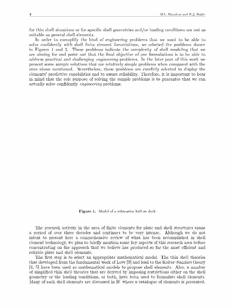
In order to exemplify the kind of engineering problems that we want to be able tosolve con�dently with shell �nite element formulations, we selected the problems shownin Figures 1 and 2. These problems indicate the complexity of shell modeling that weare aiming for and point out that the �nal objective of our formulations is to be able toaddress practical and challenging engineering problems. In the later part of this work wepresent some sample solutions that are relatively simple problems when compared with theones above mentioned. Nevertheless, those problems are carefully selected to display theelements' predictive capabilities and to assure reliability. Therefore, it is important to bearin mind that the sole purpose of solving the sample problems is to guarantee that we canactually solve con�dently engineering problems.
Figure 1. Model of a submarine hull on dock
The research activity in the area of �nite elements for plate and shell structures spansa period of over three decades and continues to be very intense. Although we do notintent to present here a comprehensive review of what has been accomplished in shellelement technology, we plan to brie y mention some key aspects of this research area beforeconcentrating on the approach that we believe has produced so far the most eÆcient andreliable plate and shell elements.
The �rst step is to select an appropriate mathematical model. The thin shell theoriesthat developed from the fundamental work of Love [3] and lead to the Koiter{Sanders theory[4, 5] have been used as mathematical models to propose shell elements. Also, a numberof simpli�ed thin shell theories that are derived by imposing restrictions either on the shellgeometry or the loading conditions, or both, have been used to formulate shell elements.Many of such shell elements are discussed in [6] where a catalogue of elements is presented.

Finite Element Analysis of Shell Structures 5

6 M.L. Bucalem and K.J. Bathe
The approach of degenerating the shell from a solid is a very attractive alternative to theuse of a thin shell theory. In this approach the shell behavior is described by imposing judi-ciously chosen kinematic and mechanical assumptions on the three{dimensional continuummechanics conditions. The resulting theory corresponds for plate bending situations to theReissner{Mindlin plate theory. This approach has been �rst presented, in the context of ashell element formulation by Ahmad et. al. [7] and has some key features that make it verysuitable for shell �nite element constructions, namely:
� The formulation is applicable to any shell geometry.� The formulation is adequate for thin and thick situations.� The formulation leads to C0 conforming displacement-based elements.� The formulation uses only engineering nodal point degrees of freedom such as displace-ments and rotations.
Shell elements based on this approach have been formulated for general nonlinear analysis(material and geometric nonlinear) by Ramm [8] and Bathe and Bolourchi [9].
Although the pure displacement-based formulation of these elements has all the abovementioned appealing features, which are very desirable if the elements are to be used inengineering practice, they do su�er from the serious de�ciency of membrane and shearlocking. The locking e�ects are devastating for lower{order elements, and even for higher{order elements they severely reduce the potential predictive capability of the elements.
A number of approaches and techniques have been proposed to overcome these diÆcul-ties. The simplest one, however unsuccessful, is the use of uniform and selective reducedintegration. In general the URI (uniform reduced integrated) elements possess spurious zeroenergy modes, and although in some cases they may provide accurate solutions, in othercases a global mechanism may form due to the collective action of the spurious zero energymodes causing rank de�ciency (or almost rank de�ciency) of the global sti�ness matrix.Even if a global mechanism does not arise, a near{mechanism might be activated whichleads to unacceptable answers. The recommendation of disregarding solutions that havebeen a�ected by spurious energy modes is almost impossible to observe since, when thesolution of the problem is not known, the judgment of whether a solution is \good" or notis very diÆcult to make. The SRI (selective reduced integrated) elements, although to asmaller degree, su�er from the same de�ciencies as the URI elements and in some casesshow very low convergence rates. Both types of elements are quite sensitive to geometricdistortions. The above considerations make clear that the use of reduced integration is anunreliable technique to deal with locking e�ects. Nevertheless, the literature is rich in uni-form and selective reduced integrated elements for plates and shells. We refer here just tothe early works on reduced integration [10, 11, 12]. We note that in some cases it is possibleto show a total equivalence between the use of reduced integration and a mixed formulation[13, 14]. In such an event reduced integration may be an eÆcient way of implementing amixed method but the analysis of whether the formulation is a good formulation or not hasto be made in the context of mixed methods.
Belytschko and co-workers developed the concept of spurious mode control [15, 16] in anattempt to use reduced integration and avoid the possibility of having spurious zero energymodes. Although successful in suppressing the spurious modes, their formulation is nottransparent, requiring the use of some numerically adjusted factors.
It is our view that the development of shell �nite elements should be guided by thefollowing requirements:
1. The elements should be reliable2. The elements should be computationally e�ective3. The element formulation should be general i.e., the elements should be applicable to:

Finite Element Analysis of Shell Structures 7
{ nonlinear analysis (geometric and material non-linear solutions),{ thick and thin plate/shell situations,{ any shell geometry
4. The formulation of the elements should be mechanistically clear and suÆciently simpleto render the elements suitable for engineering analysis.
The continuum-based degenerated shell elements satisfy requirements 3 and 4, but thelower-order elements do not satisfy requirements 1 and 2, and the higher{order 16-nodeelement does not suÆciently satisfy requirement 2, due to the e�ects of membrane andshear locking.
Ideally, considering requirements 1 and 2, the element formulation would lead to �niteelement discretizations that could be shown mathematically to be stable, convergent and tohave optimal error bounds. In plate analysis much progress has been made in this regard.Especially, the MITC family of Reissner-Mindlin plate bending elements has been developedby Bathe et.al. and has a strong mathematical foundation that assures the convergence ofthe discretizations with optimal error bounds for the displacement variables. The theoreticalfoundations of the elements can be found in [17, 18, 19, 20] and additional theoretical andnumerical results are presented in [21, 22, 23, 24, 25].
In general shell analysis, as stated in requirement 3, the situation is quite di�erent. Amathematical analysis of the type just mentioned is not available. However, a very valuablecontribution in this direction, although restricted in its applicability, has been published byPitk�aranta [26].
Since a complete mathematical theory is lacking, the following conditions should bestrictly enforced to satisfy requirement 1:
a) The elements should not have any spurious zero energy mode.b) The elements should not membrane or shear lock, when used in reasonably distorted
meshes1.c) The predictive capability of the elements should be high and relatively insensitive to
geometric distortions.
The conditions a) to c) represent a major diÆculty in arriving at reliable shell elements.The conditions regarding locking and spurious energy modes are further discussed in Section3.3. It is also well known that many shell elements perform well when of regular (sayrectangular) shape but their predictive capabilities deteriorate rapidly as the elements aregeometrically distorted. Since (in order to model a complex shell geometry) distortedelements are invariably employed in engineering practice, it is important to assure thatelement distortions do not lead to a signi�cative loss in solution accuracy.
Of course, insight into element behavior and the use of numerical experiments areimportant in the design of elements that satisfy the above conditions. It is our view that anelement which fails any one of these conditions should not be used in engineering practice.
The Mixed Interpolation of the Tensorial Components (MITC) approach has been usedsuccessfully to propose shell elements that satisfy the above conditions and requirement 2.Also, the formulation of the MITC elements preserves the essential and appealing character-istics of the continuum-based degenerated shell elements, therefore satisfying requirements3 and 4.
The approach of mixed interpolation of tensorial components for shell elements �nds itsroots in the work of Dvorkin and Bathe [21], who developed a 4-node general shell element,called the MITC4 element. This element degenerates to the MITC4 plate bending element
1 We shall in the following say that an element does not membrane or shear lock if such phenomena arenot observed as long as the element is not severely distorted.

8 M.L. Bucalem and K.J. Bathe
when the geometry is at, the analysis is linear and the plate is subjected to transverseloading only, and then is closely related to the elements proposed by Hughes and Tezduyar[27] and MacNeal [28]. However, the MITC4 element was originally proposed for shellanalysis and this is where assumed covariant strain component �elds were �rst introduced.The subsequent developments undertaken with the MITC approach for general shell analysisare discussed in sections 3.3 and 4.
In the following sections we �rst discuss the continuum mechanics formulation of thedisplacement-based shell elements for general nonlinear analysis. This formulation is ob-tained in Section 2 by a consistent linearization of the principle of virtual work whichcontains the kinematic and stress assumptions of the three-dimensional large deformationbehavior of a general shell. The resulting element formulation presented on Section 3 con-siders large displacements and rotations.
Since the pure displacement formulation even for higher-order elements do not fullysatis�es the requirements that were outlined earlier, the formulation is extended in Section4 to a mixed interpolation of strains and displacements to arrive at e�ective elements. Insection 4.2 we summarize the mathematical theory of the MITC plate bending elements.This mathematical analysis besides providing a framework to construct optimally convergentplate bending elements, gives much insight into the shear locking phenomenon aiding, ofcourse, the construction of new shear locking free shell elements. In any case, the linearplate bending problem is per se an important mathematical model for practical applicationsand deserves a special treatment. In Section 5, we discuss the speci�cation of the boundaryconditions, where we give speci�c attention to the di�erences that arise due to boundarylayer e�ects when imposing di�erent constraints for simply supported or clamped conditions.However, to investigate the behavior of the elements in the analysis of general shells andwhen used in geometrically distorted forms, recourse is necessary to numerical studies.Therefore, we present in Section 6 a selection of numerical results that give insight into thepredictive capabilities of the elements discussed in this work.
2. CONTINUUM MECHANICS FORMULATION OF DISPLACEMENT-
BASED ELEMENTS
The formulation of the shell elements is based on the use of the general principle of virtualwork for 3-D continua modi�ed for the stress-strain and kinematic assumptions of shellbehavior. In the following discussion we therefore present �rst the use of the general principleof virtual work in 3-D large deformation analysis and then discuss the speci�c modi�cationsused for shell analysis.
2.1 Principle of Virtual Work
The large deformation analysis requires in general a step-by-step incremental solution. Thebasic continuum mechanics equation used in this solution is the linearized incremental formof the principle of virtual work [29].
To establish the governing equations, we make the fundamental assumption that theresponse of the continuum can be described by the incremental potential,
dt0W =t
0~Sijdt
0~�ij (1)
where the t0~Sij are the contravariant components of the 2nd Piola-Kirchho� stress tensor
and the t0~�ij are the covariant components of the Green-Lagrange strain tensor, both at time
t and referred to the original con�guration (that corresponds to time 0). The variable t0W
represents the energy per unit of original volume.
Finite Element Analysis of Shell Structures 9
The description postulated in (1) holds, of course, for elastic materials and also for in-elastic materials widely considered in engineering practice (for example, von Mises plasticityand creep).
A consequence of the assumption in (1) is that
t
0~Sij =
@t0W
@t0~�ij(2)
The principle of virtual work is given as [29]Z0V
t
0~Sij Æt
0~�ij d
0V = tR (3)
where tR is the total external virtual work due to surface and body forces.Using (2) we can write (3) as
Æ
Z0V
t0W d 0V = tR (4)
and it follows that the linearization of the principle of virtual work expression (for theincremental solution) will for deformation-independent loading lead to symmetric tangentsti�ness matrices.
If the loading is deformation-dependent (i.e., tR depends on the deformations from time0 to time t) a non-symmetric contribution to the sti�ness matrix may be obtained whenlinearizing (4).
In fact, Schweizerhof and Ramm [30] have studied the case of pressure loading, thatusually leads to a displacement dependent loading. In such cases the pressure is modeledas a follower loading i.e., the direction of the pressure loading is considered to be alwaysnormal to the deformed surface on which the pressure is acting. In order to brie y outlinehow a follower pressure loading is introduced in the formulation, consider that part of thetotal external virtual work tR is due to the displacement dependent pressure loading, anddenote it by tRp. Then we can write
tRp =
ZtSp
tpi Æui dtSp (5)
where tSp is the surface area at time \t" on which the pressure is acting and tpi is the ith
component of the pressure which can be de�ned as
tpi =t� lf tni (6)
Here t� is the load multiplier for proportional loading, lf = lf (lx1;l x2;
l x3) representsthe spatial loading distribution and tni is the ith component of the unit normal vector tothe surface at time t. Regarding lf two cases can be identi�ed. For l = t i.e., tf =t f (tx1;
t x2;t x3), the pressure loading at time \t" at a particular point depends on the
spatial position occupied by the point at time \t". This case is referred to as space attachedload. For l = 0 i.e., 0f = 0f (0x1;
0 x2;0 x3), the pressure loading at a particular point
depends on the position occupied by the point in the initial con�guration. This case isreferred to as body attached loading.
Due to the displacement dependency of tRp as given in Eqs. (5) and (6) its incrementalloading term will have the usual type of load vector plus a contribution to the tangentsti�ness as detailed in [30]. This contribution is in general non{symmetric characterizinga non-conservative type of loading (in some cases, e.g., for particular boundary conditions,this matrix contribution may be symmetric). The purpose of these remarks regarding
10 M.L. Bucalem and K.J. Bathe
displacement dependent pressure loading was merely to hint how deformation-dependentloading may lead to non-symmetric contributions to the tangent sti�ness matrix.
In practice, it may, however, be more eÆcient to neglect the non-symmetric sti�nessmatrix contribution and simply include the deformation dependency of the loading in theiteration vectors.
The incremental form of the principle of virtual work for the stress solution at time t+�tis obtained by performing a Taylor series expansion in terms of the displacements about thestate at time t. Then substituting the interpolations for the displacement components assummarized in Section 2.2 yields the equations of motion of a �nite element
tK u = t+�tR �tF (7)
where u stores the incremental nodal point displacements ( and nodal point rotations in thecase of a shell element) and tK is the tangent sti�ness matrix; the vector t+�tR is the loadvector corresponding to time t+�t , and tF is the vector of nodal point forces correspondingto the element stresses at time t. Here
tFi =@
@ui
�Z0V
t
0W d 0V
�(8)
tKij =@tFi
@uj(9)
and using chain di�erentiation
tFi =
Z0V
t
0~Skl
@t0~�kl
@uid 0V (10)
tKij =
Z0V
0Cklrs
@t0~�kl
@ui
@t0~�rs
@ujd 0V +
Z0V
t
0~Skl @
2 t0~�kl
@ui @ujd 0V (11)
In the analysis of continua using isoparametric �nite elements the displacements are inter-polated in a �xed Cartesian coordinate system as
tui = hLtuLi (12)
where tuLi is the nodal point displacement in the coordinate direction i at node L and timet. Also
t0~�kl =
1
2
�t0xb;k
t
0xb;l � Ækl
�(13)
where t0xb;l =
@txb
@0xland Ækl is the Kronecker delta . Hence
@ t0~�kl
@uLi=
1
2
�t
0xi;k 0hL;l + t
0xi;l 0hL;k
�(14)
and@2 t
0~�kl
@uLi @uMj
=1
2(0hL;k 0hM;l + 0hL;l 0hM;k) Æij (15)
where the uLi ; uMi are the incremental nodal point displacements identi�ed earlier as ui.
In the analysis of shells we use
t
0~�kl =
1
2
�tg
k�
tgl�
0gk
�0g
l
�(16)
Finite Element Analysis of Shell Structures 11
wheretg
i=
@tx
@ri; 0g
i=
@0x
@ri(17)
and r1 � r; r2 � s and r3 � t where (r; s; t) are the usual isoparametric coordinates . Inthis case the ui correspond to translational and rotational degrees of freedom; hence thedi�erentiations required in (10) and (11) are more diÆcult to evaluate and depend on thespeci�c rotational degrees of freedom used.
2.2 Shell Assumptions
The assumptions used for the shell kinematic and stress conditions are a generalization ofthe Reissner-Mindlin plate theory [29].
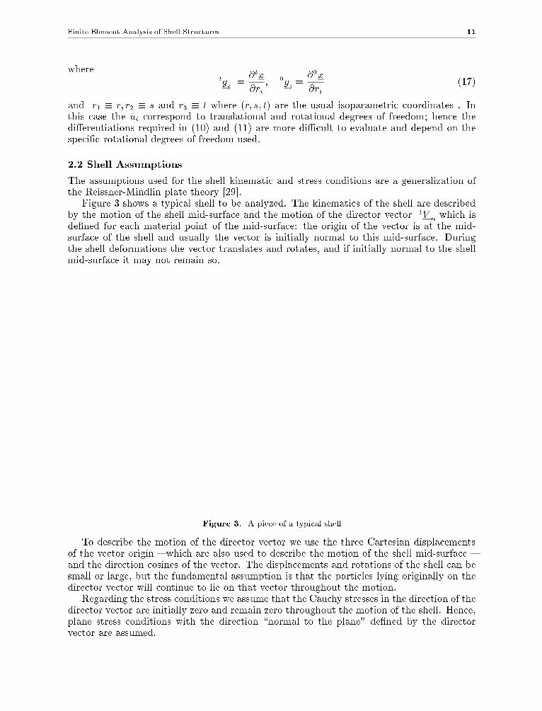
Figure 3 shows a typical shell to be analyzed. The kinematics of the shell are describedby the motion of the shell mid-surface and the motion of the director vector tV
n which isde�ned for each material point of the mid-surface: the origin of the vector is at the mid-surface of the shell and usually the vector is initially normal to this mid-surface. Duringthe shell deformations the vector translates and rotates, and if initially normal to the shellmid-surface it may not remain so.
Figure 3. A piece of a typical shell
To describe the motion of the director vector we use the three Cartesian displacementsof the vector origin { which are also used to describe the motion of the shell mid-surface {and the direction cosines of the vector. The displacements and rotations of the shell can besmall or large, but the fundamental assumption is that the particles lying originally on thedirector vector will continue to lie on that vector throughout the motion.
Regarding the stress conditions we assume that the Cauchy stresses in the direction of thedirector vector are initially zero and remain zero throughout the motion of the shell. Hence,plane stress conditions with the direction \normal to the plane" de�ned by the directorvector are assumed.

12 M.L. Bucalem and K.J. Bathe
3. DISPLACEMENT{BASED SHELL ELEMENTS
The formulation of the displacement-based shell elements is based on the principle of virtualwork with the kinematic and stress assumptions summarized above, and on the interpolationof the coordinates of the material particles of the shell.
3.1 Interpolation of Coordinates and Displacements
Figure 4 shows a typical shell element. The coordinates of any material particle at time tare [29]
txi = hktxki +
t
2ak hk
tV k
ni (18)
where the hk are the usual 2-D isoparametric interpolation functions in (r; s), ak is thethickness of the element at node k measured along the direction of the director vector, thetxki are the coordinates of the nodal point k and the tV k
ni are the direction cosines of the
director vector tV k
n at the nodal point k. We note that the material particle coordinates,the nodal point coordinates and the directions of the director vectors are all measured inthe stationary coordinate system, xi; i = 1; 2; 3. For the element in Figure 4 the number ofnodes is sixteen and hence in Eq. (18) k = 1; : : : ; 16:
Figure 4. Typical shell element. The direction of the isoparametric coordinate t is given bythe director vector t
V n(r; s)
Equation (18) and Figure 4 show that the shell element geometry is interpolated using theintrinsic coordinate variables r; s and t. We note that the variable t;�1 � t � 1; is measured
Finite Element Analysis of Shell Structures 13
in the direction of the director vector tV n and the variables r and s;�1 � r; s � +1, aremeasured in the mid-surface of the shell element.
For the de�nition of the stress-strain law, the direction of \zero normal stress" is takento be the t-direction and the stress-strain law at any material particle is established in the(r; s; t) system, where unit vectors in these directions are
er = (es � et) = k es � et k2 (19)
es = et � er (20)
and er, es, et are the unit vectors in the r, s and t directions.It is clear that with the coordinate interpolation for any time t given by Eq. (18), the
displacements at any time can directly be evaluated; for example,
tui =txi �
0xi (21)
= hktuki +
t
2akhk
�tV k
ni �0V k
ni
�(22)
In the �nite element formulation we linearize the response about the con�guration attime t (see Eqs. (10) and (11) ) and want to use nodal point displacements and rotations.
Hence, we need to relate the change in tV k
n to rotations at the nodal point k. This is
achieved by introducing two auxiliary axes tV k
1and tV k
2which together with tV k
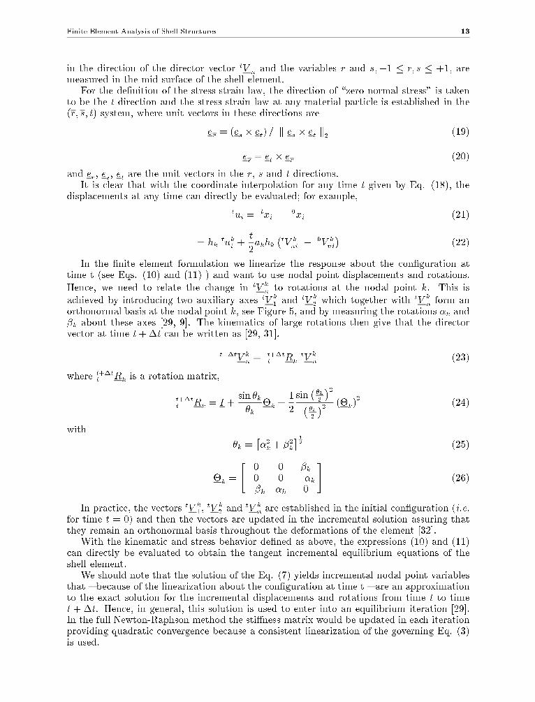
n form anorthonormal basis at the nodal point k, see Figure 5, and by measuring the rotations �k and�k about these axes [29, 9]. The kinematics of large rotations then give that the directorvector at time t+�t can be written as [29, 31].
t+�tV k
n =t+�t
t Rk
tV k
n (23)
where t+�tt Rk is a rotation matrix,
t+�t
t Rk = I +sin �k
�k�k +
1
2
sin��k2
�2��k
2
�2 (�k)2
(24)
with
�k =��2k + �2k
� 12 (25)
�k =
"0 0 �k0 0 ��k
��k �k 0
#(26)
In practice, the vectors tV k
1, tV k
2and tV k
n are established in the initial con�guration (i.e.for time t = 0) and then the vectors are updated in the incremental solution assuring thatthey remain an orthonormal basis throughout the deformations of the element [32].
With the kinematic and stress behavior de�ned as above, the expressions (10) and (11)can directly be evaluated to obtain the tangent incremental equilibrium equations of theshell element.
We should note that the solution of the Eq. (7) yields incremental nodal point variablesthat { because of the linearization about the con�guration at time t { are an approximationto the exact solution for the incremental displacements and rotations from time t to timet + �t. Hence, in general, this solution is used to enter into an equilibrium iteration [29].In the full Newton-Raphson method the sti�ness matrix would be updated in each iterationproviding quadratic convergence because a consistent linearization of the governing Eq. (3)is used.
14 M.L. Bucalem and K.J. Bathe
Figure 5. De�nition of rotational degrees of freedom �k and �k
3.2 Nodal Point Variables
The nodal point variables in the solution are the incremental displacements into the Carte-
sian coordinate directions and the rotations �k and �k about the currenttV k
1and tV k
2axes.
We note that these axes change direction during the large displacement motion.There are hence �ve natural nodal point variables at each shell node. However, some
special considerations are necessary at shell nodes,
(i) that are shared by two or more shell elements,(ii) that connect also to other kinds of �nite elements, or(iii) at which rotational boundary conditions (rotations or moments ) are prescribed.
Namely, at these nodes it may be more convenient to use six degrees of freedom.Consider case (i). If a single director vector is used at the shell node shared by two
or more shell elements, only �ve degrees of freedom describe the kinematic behavior (since
no sti�ness is calculated for the rotation about the director vector tV k
n). In practice, theuser would prescribe that only �ve degrees of freedom shall be used at such a node andthe program would automatically assign only a single director vector (as the average ofthe vectors normal to the mid-surfaces of the shell elements at that node). If a smoothshell surface is modeled, the assumption of a single director vector at the node is quiteappropriate (see Figure 6a). However, at a node of a corner or edge of shell surfaces, asingle director vector may not represent the desired model (see Figure 6b) and here theanalysis could employ di�erent director vectors for each element. This requires the use ofsix degrees of freedom at the node (see Figure 6c). In practice, the user would assign sixdegrees of freedom at a corner or edge node if the model of Figure 6.c is to be used, andthe program would then establish automatically di�erent director vectors for each elementat that node.

Finite Element Analysis of Shell Structures 15
(a) Single director vector at a node shared by two elements modeling a smooth shell surface
(b) Single director vector at a node shared by two elements modeling a shell intersection
(c) Element individual director vectors at a node shared by two shell elements modeling ashell intersection
Figure 6. Director vector at nodes shared by elements
Considering cases (ii) and (iii) the use of six degrees of freedom at the shell node maybe necessary because in (ii) the other �nite elements (e.g., beam elements) may carryrotational degrees of freedom in three global (or skew) coordinate directions and in (iii)speci�c rotational boundary conditions in global (or skew) coordinate directions may need
16 M.L. Bucalem and K.J. Bathe
to be imposed (for example, to enforce symmetry conditions). In each of these cases it ishowever important when building the model to keep in mind that the shell element has only
rotational sti�ness about its tV k
1and tV k
2axes.
Another convenient way to model shell intersections, such as the intersection schemat-ically displayed in Figure 6b, is to use transition elements. These elements [29, 33] areformulated with shell mid-surface nodes and top and bottom surface nodes. The shell mid-surface nodes carry the usual shell degrees of freedom whereas the top and bottom surfacenodes carry only translational degrees of freedom. Solutions with these transition elementscan also yield more accurate results [33].
3.3 Element Performance
The above displacement formulation is applicable to elements with a varying number ofnodes. However, in practice, only the cubic 16-node quadrilateral element, referred to asthe 16-node displacement-based element, or higher order elements, can be used for generalshell analysis, because the lower-order elements \lock" due to spurious shear and membranestrains. Even the 16-node displacement-based element can show a locking behavior. The 16-node displacement-based element when distorted and/or curved can display a poor predictivecapability for coarse meshes. This is due largely to the e�ects of membrane and shear lockingthat are increasingly important as the element is curved and distorted.
Shear locking is due to the inability of the elements (with the �nite element interpolationused) to represent the condition of zero transverse shear strains and still preserve enoughelement degrees of freedom to permit a good approximation.This condition of zero transverseshear strains is progressively enforced in the �nite element solutions as the thickness of theplate/shell becomes smaller, being totally enforced in the limit. When the only �nite elementsolution that satis�es the zero shear strain condition corresponds to zero nodal displacementseverywhere the oversti�ening of the solutions can be very large even for �nite thicknesses.A classical example of this situation is the case when lower-order elements are subjected toa bending moment only.
Even in the cases where zero shear strains can be represented with non-zero nodaldisplacement, convergence may become very slow since the restricted �nite element spacethat leads to zero shear stresses may be much smaller than the original �nite element space.
Membrane locking appears in curved structures due to the inability of the elements torepresent zero membrane states. Membrane locking will be an issue in cases when the limitsolution(thickness tending to zero) corresponds to zero membrane strains.
As already mentioned, membrane locking occurs, of course, only in curved elements.However, in geometrically nonlinear analysis, elements which are initially at may becomesigni�cantly curved during the incremental solution and may therefore only membrane lockas the deformations increase.
In the above discussion we assumed that the element sti�ness matrices are evaluated with\full" numerical integration: this order of numerical integration is such that for geometricallyundistorted elements the exact sti�ness matrices are calculated. If this same integrationorder is used to evaluate the sti�ness matrices of geometrically distorted elements, theerror in the numerical evaluation is not very signi�cant as long as the element distortionsare reasonable. To relieve the \locking" behavior of the low-order displacement-based shellelements, relatively simple schemes of reduced and selective numerical integration have beenproposed [10, 12]. Such approaches lead to computational eÆciency in the evaluation of theelement sti�ness matrix and also to overall solution e�ectiveness in the analysis of certainproblems. However, if, as already mentioned in the Introduction, an element sti�ness matrixcontains a spurious zero energy mode (such as reported in [34]) the element is interestingfor research purposes but unacceptable for practical analysis because it is not reliable.
To suppress the spurious zero energy modes, Belytschko and co-workers proposed anumerical control that can lead to eÆcient solutions and that has also been related to

Finite Element Analysis of Shell Structures 17
a variational basis [15, 16]. A shortcoming of these elements is that numerical controlparameters have to be selected and that their performance is quite sensitive to elementgeometric distortions.
An e�ective approach to formulate reliable and quite eÆcient lower-order shell elementsis to use a mixed interpolation on strains and displacements. This approach is closelyrelated to mixed and hybrid formulations but it is computationally much more e�ective.To construct general elements, Bathe and Dvorkin introduced a mixed interpolation on thetensorial components of displacements and strains [21, 2] and arrived at a 4-node and a8-node element that do not shear or membrane lock, that do not contain spurious zeroenergy modes and that display good accuracy characteristics in general analysis. Similarformulative approaches were then also used for example by Huang and Hinton [35], Parkand Stanley [36] and Jang and Pinsky [37] to propose nine node shell elements. Huangand Hinton used a local Cartesian system to separate bending and membrane strains andmixed-interpolated only the membrane part. The transverse shear strains were evaluatedand mixed-interpolated in the natural co-ordinate system. Park and Stanley used assumedphysical strain component �elds that were derived from special assumptions on the strainsalong selected coordinate lines. Jang and Pinsky assumed covariant strain components innatural coordinates for both the in-layer and transverse shear strains. These approaches offormulation are similar to the approach used in [16] and also in this work, but the actualdetailed assumptions employed results, of course, in quite di�erent elements.
Recently, Bucalem and Bathe [38] proposed two additional elements based on the mixedinterpolation of the tensorial components, a 9-node element and a 16-node element, thatdisplay the numerical eÆciency and reliability of the 4-node and 8-node elements mentionedabove.
4. MIXTED INTERPOLATION
4.1 Mixed Interpolated General Shell Elements
We stated in Section 3 that the governing equations of the displacement-based shell ele-ments are obtained by introducing the kinematic shell behavior through the �nite elementinterpolations assumptions, both for the geometry and for the displacement variables in theevaluation of the covariant strain components t
0~�ij: The tangent sti�ness matrix tKij may
then be readily obtained using Eq. (11). However, as has already been pointed out, theresulting element formulations display membrane and shear locking behavior.
The key step of the mixed interpolation of the tensorial components approach is to de�neassumed strain component �elds that are linked with the displacement variables and thatlead to element formulations that are free from membrane and shear locking diÆculties.
In order to make precise the mixed formulation let us denote by t0~�DIij the strain compo-
nents obtained from the �nite element interpolation assumptions both for the geometry anddisplacement variables. The superscript DI stand for \direct" interpolation using the ge-ometry and displacement �nite element interpolation assumptions. The mixed interpolatedelements are constructed using t
0~�ASij in place of t
0~�DIij , where the superscript AS indicates that
assumed strain �elds are used.The de�nition of how the assumed strain �elds relate to the directly interpolated strain
�elds actually characterizes a particular element formulation. The success or failure ofan element formulation in avoiding membrane and shear locking is entirely related to thede�nition of the assumed strain �elds and how they relate to the usual strain �elds.
For the plate bending problem a mathematical theory guides the selection of appropriateassumed strain �elds. The discussion of these mathematical ideas will be developed tosome extent in Section 4.2. Besides guiding the construction of optimally convergent platebending elements this mathematical theory provides much understanding and insight intothe shear locking phenomenon.
18 M.L. Bucalem and K.J. Bathe
The mixed interpolated shell �nite elements that will be presented here have beendeveloped based on insight into element behavior and the use of numerical experimentation.
Let us consider the construction of the assumed strain �elds for speci�c elements. Weomit temporarily, merely for ease of notation, the subscripts and superscripts relating totimes (0; t) in the strain expressions.
We use the convected coordinate system that is de�ned element-wise by the elementisoparametric coordinates r; s and t as shown in Figure 3 with the following convention forindicial notation: r1 � r; r2 � s and r3 � t:
Considering the kinematical shell assumptions implicitly de�ned in Eq. (18), the straintensor can be written as
�DI = ~�DIrr g
rgr + ~�DIss g
sgs + ~�DIrs
�grgs + gsgr
�+
+ ~�DI
rt
�grgt + gtgr
�+ ~�DI
st
�gsgt + gtgs
� (27)
or
�DI = �DI
IL + �DI
RT + �DI
ST (28)
where �DIIL is the in-layer part of the strain tensor and �DI
RT and �DIST the transverse shear
strain parts, with the following de�nitions:
�DI
IL = ~�DI
rr grgr + ~�DI
ss gsgs + ~�DI
rs
�grgs + gsgr
�(29)
�DI
RT = ~�DI
rt
�grgt + gtgr
�(30)
�DI
ST = ~�DI
st
�gsgt + gtgs
�(31)
One way of de�ning a mixed interpolation of the strains is to use the previous decompo-sition and write �AS, the assumed strain tensor as,
�AS = �ASIL + �ASRT + �ASST (32)
where �ASIL is the assumed in-layer strain part and �ASRT and �ASST are the assumed transverseshear strain parts.
Each assumed strain part is obtained by evaluating the corresponding directly interpo-lated strain part at some selected points, called tying points, and interpolating from thesevalues to de�ne the assumed strain tensor part for any point in the element domain.
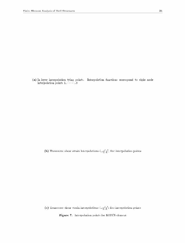
The MITC8 element is formulated with this approach and the details of this formulationwill shortly become apparent when we present the element.
Of course, to arrive at the sti�ness matrix using Eq. (11) each particular assumedcovariant strain component can be evaluated using
~�ASij = gi� �AS � g
j(33)
Another approach that has been used to formulate mixed interpolated shell elements isto de�ne assumed strain �elds for each covariant strain component. In fact, for each straincomponent ~"ij we de�ne a set of points, k = 1; : : : ; nij, by specifying for each point k itsnatural coordinates r = rk, s = sk and t. These points are also called tying points.
Now the assumed covariant strain component ~"ASij is de�ned as
~"ASij (r; s; t) =
nijXk=1
hijk (r; s)~"DI
ij (rk; sk; t) (34)

Finite Element Analysis of Shell Structures 19
where hijk(r; s) are interpolation functions (polynomials in r and s) associated with the strain
component ~"ij such that
hijk jl := hijk (rl; sl) = Ækl; l = 1; : : : ; nij (35)
and denoting
~"DI
ij jk := ~"DI
ij (rk; sk; t) and ~"ASij jk := ~"ASij (rk; sk; t) (36)
it follows
~"ASij jk = ~"DI
ij jk; k = 1; : : : ; nij (37)
Of course, this selection is the reason why the nij points are called tying points.
4.1.14.1.1 The MITC8 elementThe MITC8 element
The MITC8 element construction follows the �rst approach, outlined in the previous section,i.e., assumed strain �elds are de�ned considering the interpolation of the in-layer andtransverse shear strain parts.
The assumed in-layer strain �elds are de�ned by
�ASIL =
8Xk=1
hILk �DI
IL jk (38)
where the hILk are the usual 8-node element interpolation functions corresponding to thepoints k = 1; :::; 8 identi�ed in Figure 7a and for k = 1; : : : ; 4
�DI
IL jk= ~�DI
rr grgr jk +~�DI
ss gsgs jk +~�DI
rs
�grgs + gsgr
�jk
For k = 5 and 7
�DI
IL j5 = ~�DI
ss gsg s j5 +
�gr�
�1
2
��DI
j1 +�DI
j2��� g
r
�g rg r j5
+
�gr�
�1
2
��DI
j1 +�DI
j2��� g
s
��g rg s + g sg r
�j5
(39)
�DI
IL j7 = ~�DI
ss gsg s j7 +
�gr�
�1
2
��DI
j3 +�DI
j4��� g
r
�g rg r j7
+
�gr�
�1
2
��DI
j3 +�DI
j4��� g
s
��g rg s + g sg r
�j7
(40)
where
gs� g
s; g
t� g
t(41)
gr= g
r� �g
s; � =
grs
gss(42)
20 M.L. Bucalem and K.J. Bathe
and for i = 6 and 8
�DI
IL j6 = ~�DI
rr grg rj6 +
�gs�
�1
2
��DI
j2 + �DI
j3��� g
s
�g sg sj6+
+
�gr�
�1
2
��DI
j2 + �DI
j3��� g
s
��g rg s + g sg r
�j6
(43)
�DI
IL j8 = ~�DI
rr grg r j8 +
�gs�
�1
2
��DI
j1 +�DI
j4��� g
s
�g sg s j8 +
+
�gr�
�1
2
��DI
j1 +�DI
j4��� g
s
��g rg s + g sg r
�j8
(44)
wheregr� g
r; g
t� g
t(45)
gs= g
s� �g
r; � =
grs
grr(46)
This interpolation avoids membrane locking and does not introduce spurious zero energymodes.
The assumed shear strains are de�ned by
~�ASrt grgt =
4Xk=1
hRTk ~�DI
rt grgtjk + hRT5
�1
2
�~�DI
rt jRA + ~�DI
rt jRB��
grgtj5 (47)
and
~�ASst gsgt =
4Xk=1
hSTk ~�DI
st gsgtjk + hST5
�1
2
�~�DI
st jSA + ~�DI
st jSB��
gsgtj5 (48)
with the interpolation functions hRTk and hSTk corresponding to the points in Figure 7.Note that in (47) and (48) the mean values of the covariant strain components sampledat points RA and RB , and SA and SB , are used for the �fth interpolation functions.This corresponds to some degree to the theoretical prediction that for high-order elementsweighted integrals of the transverse shear strain components should be e�ective in tying thestrain interpolations to the nodal point variables (see Section 4.2).
The above shear strain interpolation prevents shear locking and also does not result intospurious zero energy modes. The element sti�ness matrix is evaluated using 3 � 3 Gaussintegration corresponding to the r- and s- directions.
4.1.24.1.2 The MITC4, MITC9 and MITC16 elementsThe MITC4, MITC9 and MITC16 elements
In the formulation of the MITC4, MITC9 and MITC16 elements the assumed strain �elds arede�ned as in Eq. (34). Therefore, each covariant strain component has its own interpolationand tying scheme.
For the MITC4 element, only the transverse shear strains are mixed interpolated and thetying points are shown in Figure 8. We note that the selection of the tying points completely
de�nes the assumed interpolation scheme, since the hijk (r; s) functions are products ofLagrange polynomials with the property given in (35). The MITC4 element formulationfully �ts the framework of element construction described in this section in which eachindividual covariant strain component is interpolated because, regarding the interpolationof the in-layer strains, we could formally say that the assumed strain �elds for the in-layerstrains are identical to the directly interpolated strain �elds.
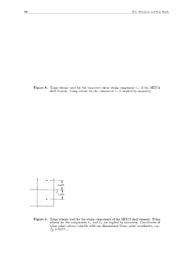
The choice of tying points for the 9-node element is given in Figure 9 and the choice forthe 16-node element is presented in Figure 10.
Finite Element Analysis of Shell Structures 21
(a) In-layer interpolation tying points. Interpolation functions correspond to eight nodeinterpolation points 1; � � � � � � ; 8
(b) Transverse shear strain interpolations ~�rtgrgt; �ve interpolation points
(c) Transverse shear strain interpolations ~�stgsgt; �ve interpolation points
Figure 7. Interpolation points for MITC8 element
22 M.L. Bucalem and K.J. Bathe
Figure 8. Tying scheme used for the transverse shear strain component ~�rt of the MITC4shell element. Tying scheme for the component ~�st is implied by symmetry
Figure 9. Tying scheme used for the strain components of the MITC9 shell element. Tyingscheme for the components ~�ss and ~�st are implied by symmetry. Coordinates oftying points always coincide with one-dimensional Gauss point coordinates, e.g.,1p3= 0:577 : : :
Finite Element Analysis of Shell Structures 23
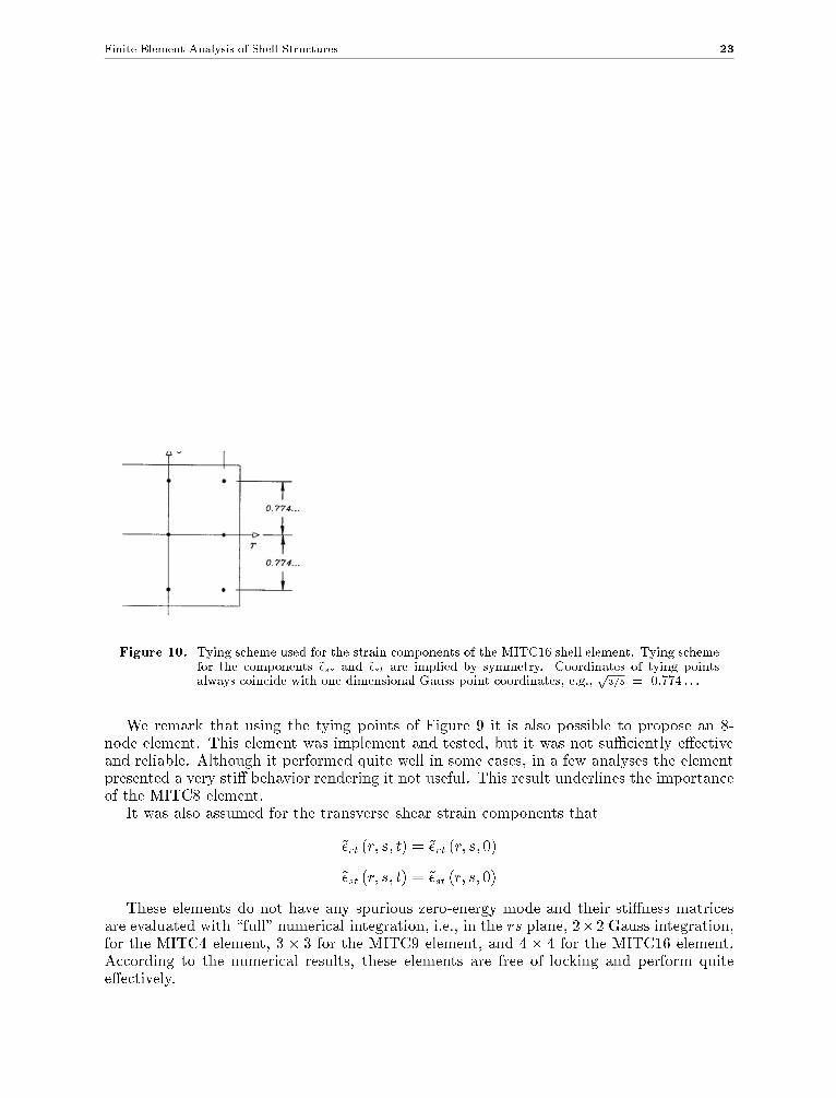
Figure 10. Tying scheme used for the strain components of the MITC16 shell element. Tying schemefor the components ~�ss and ~�st are implied by symmetry. Coordinates of tying pointsalways coincide with one-dimensional Gauss point coordinates, e.g.,
p3=5 = 0:774 : : :
We remark that using the tying points of Figure 9 it is also possible to propose an 8-node element. This element was implement and tested, but it was not suÆciently e�ectiveand reliable. Although it performed quite well in some cases, in a few analyses the elementpresented a very sti� behavior rendering it not useful. This result underlines the importanceof the MITC8 element.
It was also assumed for the transverse shear strain components that
~�rt (r; s; t) = ~�rt (r; s; 0)
~�st (r; s; t) = ~�st (r; s; 0)
These elements do not have any spurious zero-energy mode and their sti�ness matricesare evaluated with \full" numerical integration, i.e., in the rs plane, 2�2 Gauss integration,for the MITC4 element, 3� 3 for the MITC9 element, and 4� 4 for the MITC16 element.According to the numerical results, these elements are free of locking and perform quitee�ectively.

24 M.L. Bucalem and K.J. Bathe
4.2 Additional MITC Elements. The Mixed Interpolated Plate Bending Ele-
ments
The MITC4 and MITC8 elements have been constructed by insight into the predictivebehaviors to reach 4- and 8-node shell elements that are reliable and have good predictivecapabilities. The convergence behavior of the elements was originally tested by consideringpatch tests and selected plate and shell analyses.
The development of the MITC9 and MITC16 shell elements, that followed, was guidedto some extent by the previous developments of the MITC9 and MITC16 plate bendingelements. The construction of the MITC plate bending elements involves the de�nition ofassumed transverse shear strain �elds and also of tying schemes that relate the assumed anddirectly interpolated shear strains.
When developing general mixed interpolated shell elements it is also necessary to de�neassumed transverse shear strain �elds and tying conditions. These constructions can beguided by the analogous constructions for the plate bending elements. However, twocomments are in order
(i) The plate bending elements were designed to take into account the known nature of theReissner-Mindlin plate bending mathematical model. When considering general curvedshells the mathematical model is quite di�erent and it is not clear whether the optimalchoice of assumed transverse shear strain �elds is the same as for the plate model.
(ii) As will be reviewed shortly the MITC plate bending element constructions for the higher-order elements require the use of di�erent sets of degrees of freedom for the nodal pointdisplacements and the nodal point section rotations. These constructions, if followedstrictly when formulating shell elements, would lead to shell elements that are diÆcultto use in practical engineering applications. Also, for the MITC plate bending elementsnot only point-tying conditions are used but also integral-tying conditions. Integral-tying conditions are expensive, in terms of the computational e�ort, in particular ifimplemented for shell analysis.
Therefore it is justi�ed that the assumed shear strain �elds for the MITC plate andshell elements are not exactly the same. However, it is apparent that the study of thetransverse shear strain �elds for the plate elements provides valuable insight for developingthe corresponding strain �elds for shell elements.
Of course, the construction of assumed in-layer strain interpolations can not be aided bythe consideration of plate bending analysis. In order to arrive at the assumed in-layer straininterpolations for the MITC9 and MITC16 shell elements insight into element behavior andnumerical experimentation were used.
In the remaining part of this section we summarize the fundamental ideas of the math-ematical analysis of the Reissner-Mindlin linear elastic plate bending problem. We alsopresent, brie y, the MITC plate elements that have been developed. Some numerical re-sults obtained with these elements are shown as well to indicate the predictive capabilitiesof these elements.
The mathematical analysis proceeds by considering the minimization of the total poten-tial corresponding to bending of a Reissner- Mindlin plate
inf
�t3
2a��; �
�+�t
2
� �rw 20� t3 (f;w)
�(49)
� 2 B; w 2W
where B is the space of plate section rotations and W is the space of the plate transversedisplacement, t is the thickness of the plate and t3f is the transverse applied loading.The �rst term in (49) is the bending strain energy and the second term corresponds to
Finite Element Analysis of Shell Structures 25
the transverse shear strain energy. If we look for a solution in the �nite element subspacesBh � B and Wh �W; we know that in general shear locking occurs.
To avoid shear locking we need to reduce the in uence of the shear strain energy, and thisis achieved by using a space of assumed transverse shear strains �h and a projection operatorR that relates the shear strains given by �
h�rwh to the assumed strains R(�
h�rwh) in
�h: We assume further that this operator R satis�es
R rwh = rwh for all wh 2Wh (50)
and then solve instead of the discrete version of (49) the following minimization problem
inf
�t3
2a��h; �
h
�+�t
2
R�h�rwh
20
� t3 (f;wh)
�(51)
�h2 Bh; wh 2Wh
Let us consider the sequence of problems Pt each associated with a particular thicknesst, given by
Pt : inf
�1
2a��; �
�+�t�2
2
� �rw 20� (f;w)
�(52)
� 2 B; w 2W
and analogously the sequence corresponding to (51)
Pth : inf
�1
2a��h; �
h
�+�t�2
2
R�h�rwh
20
� (f;wh)
�(53)
�h2 Bh; wh 2Wh
Of course, we now have to select Bh;Wh;�hand the operator R such that (53) yields �niteelement solutions that are convergent to the solution of the continuous problem governedby (52).
Although we would like to consider the convergence of the solution of (53) to (52) for arange of values t physically possible, in order to choose the variables Bh;Wh;�h and R itis expedient to consider the limit case of t = 0. The convergence analysis is then, of course,not complete but it does yield important information on what �nite element spaces andoperators R will be e�ective.
Therefore, for the limit problem, (52) becomes
inf�=rw
�1
2a��; �
�� (f;w)
�(54)
and (53) becomes
infR�
h=rwh
�1
2a��h; �
h
�� (f;wh)
�(55)
Considering the construction of the discrete spaces Bh;Wh;�h we recognize that given apair �,w of smooth fuctions such that
� = rw (56)
26 M.L. Bucalem and K.J. Bathe
we want to �nd a corresponding pair �h2 Bh,wh 2Wh such that
R(�h�rwh) = R �
h�rwh = 0 (57)
or
R �h= rwh (58)
with �h,wh \close" to �,w (i.e., �
h,wh approximate �,w with optimal error bounds). If this
holds true and if R is \close" to the identity operator, then the solution of (55) will be agood approximation of the solution of (54).
We note that (56) implies
rot���= 0 (59)
and analogously (58) implies
rot�R�
h
�= 0 (60)
The condition (59) is much like the condition div u = 0 to be satis�ed in the analysisof incompressible media(where u is the displacement vector), except that in (59) the rotoperator is used [39].
Taking advantage of the incompressible analysis problem it can be established thatgiven a continuous �eld � such that rot � = 0 we can �nd �
h2 Bh which is a \good"
approximation for � and that Z
rot(�h) qhd = 0 8qh 2 Qh (61)
where Bh; Qh are a \good" pair of displacement-pressure spaces for the approximation of
the incompressible medium problem.If R and �
h are chosen such thatZ
rot(�) qhd =
Z
rot(R�) qhd (62)
8� 2 Bh; 8qh 2 Qh
and if
rot�h � Qh (63)
then Eq. (61) implies the desired (60).Considering Eqs.(50) and (58) we realize that there is not much choice left to de�ne Wh.
In fact it is necessary that
rWh =�' 2 �hsuch that rot' = 0
(64)
This condition together with (50) characterizes Wh:We note that (64) together with (60) implies the existence of wh 2 Wh such that (58)
holds and since R is to be chosen as a good approximation of the identity operator
rwh = R �h' �
h' � = rw
Finite Element Analysis of Shell Structures 27
meaning that wh will be a good approximation of w.Therefore the choice of the �nite element spaces is guided by the following steps:
StepStep 11: choose Bh; Qh such that it corresponds to a \good"displacement-pressure pair forthe analysis of incompressible media. These pairs can be easily found in the literature (seefor example [49]).
StepStep 22: choose �hand R such that Eqs. (62) and (63) are satis�ed.
StepStep 33: choose Wh according to Eq. (64).
It has been established [19] that the above element construction leads to mixed inter-polated plate bending elements that have optimal convergence characteristics and thereforedo not lock.
We note that the tying, i.e., the link between the assumed strain �elds given by �h and
the directly interpolated strain �elds is given by Eq. (62).The mathematical analysis summarized above has evolved from the analysis of the
MITC4 element, that has originally been proposed for shell analysis, when used in platebending conditions. The elements that have been developed according to the mathematicalframework outlined above and that have also been numerically tested are: the MITC9 andthe MITC16 elements (quadrilateral 9- and 16-node elements); the MITC7 and MITC12elements (triangular 7- and 12-node elements). These elements are described in Figures 11,12, 13, 14 and 15. As we may observe, for the higher-order, MITC7, MITC9, MITC12and MITC16 elements, di�erent sets of degrees of freedom for transverse displacements andsection rotations are used and also integral tying conditions are present. We have alreadypointed out this fact when discussing the possible di�erences between MITC plate bendingand shell elements and the reasons why they were actually constructed in this way. Whenthe MITC9 and MITC16 shell elements are used under plate bending conditions they do notdegenerate to the MITC9 and MITC16 plate bending elements. Of course, we do not expectthat the MITC9 and MITC16 shell elements perform as well as the MITC9 and MITC16plate elements when used for plate bending problems. However, the shell elements shouldstill behave quite e�ectively in plate bending situations and, of course, not shear lock.
We present below two plate bending problems that have been modeled with the MITCplate elements. A third problem is studied where we compare the behavior of the MITCplate and shell elements in the analysis of a plate bending problem.
4.2.14.2.1 Analysis of a simply-supported square plateAnalysis of a simply-supported square plate
We consider the transverse shear stress predictions in the analysis of a square plate subjectedto uniform pressure. In this problem the transverse shear stresses display a strong boundarylayer [40]. Therefore this is an adequate test problem to assess the predictive capability ofthe elements regarding transverse shear stresses for engineering problems in which thesestresses vary rapidly.
Only a quarter of the plate needs to be discretized and we obtained a reference solutionusing graded meshes of 16{node displacement based elements (in undistorted form). The10�10 graded mesh is shown in Figure 16 and the 20�20 mesh was obtained by subdividingeach element of the 10�10 mesh into four new elements. The solutions obtained with thesemeshes showed negligible di�erences.
In Figures 17 and 18 we show the predictions, along the edge of the plate from the corner,obtained with the MITC4 and MITC9 elements and the reference solution. The stresses areevaluated at the corner of the elements using the �h spaces. The MITC element predictionsshow a good convergence to the reference solution. We note that at a suÆcient distancefrom the corner the solution corresponds to the Kirchho� solution. We also remark that foran accurate solution grading in the meshes should be used for this type of analysis [29].

28 M.L. Bucalem and K.J. Bathe
Figure 11. MITC4 plate element
4.2.24.2.2 Convergence in the analysis of an \Ad-hoc problem"Convergence in the analysis of an \Ad-hoc problem"
We consider the problem of a square Reissner-Mindlin plate of side lengths two units, seeFigure 19. The interior loading is p=0 and the imposed boundary displacement and sectionrotations correspond to:
w = sin kxeky + sin ke�k (65)
�x = k cos kxeky (66)
�y = k sin kxeky (67)
with k = 5. We note that the above equations satisfy the Reissner-Mindlin plate equationsfor any value of the thickness t, and hence represent the complete (boundary and interior)solution. There is no boundary layer [40,41], and indeed the transverse shear strains arezero.
Hence this problem is a valuable test problem in that the numerically calculated conver-gence rates should be close to the theoretically predicted rates.

Finite Element Analysis of Shell Structures 29
Figure 12. MITC9 plate element

30 M.L. Bucalem and K.J. Bathe
Figure 13. MITC16 plate element

Finite Element Analysis of Shell Structures 31
Figure 14. MITC7 plate element
32 M.L. Bucalem and K.J. Bathe
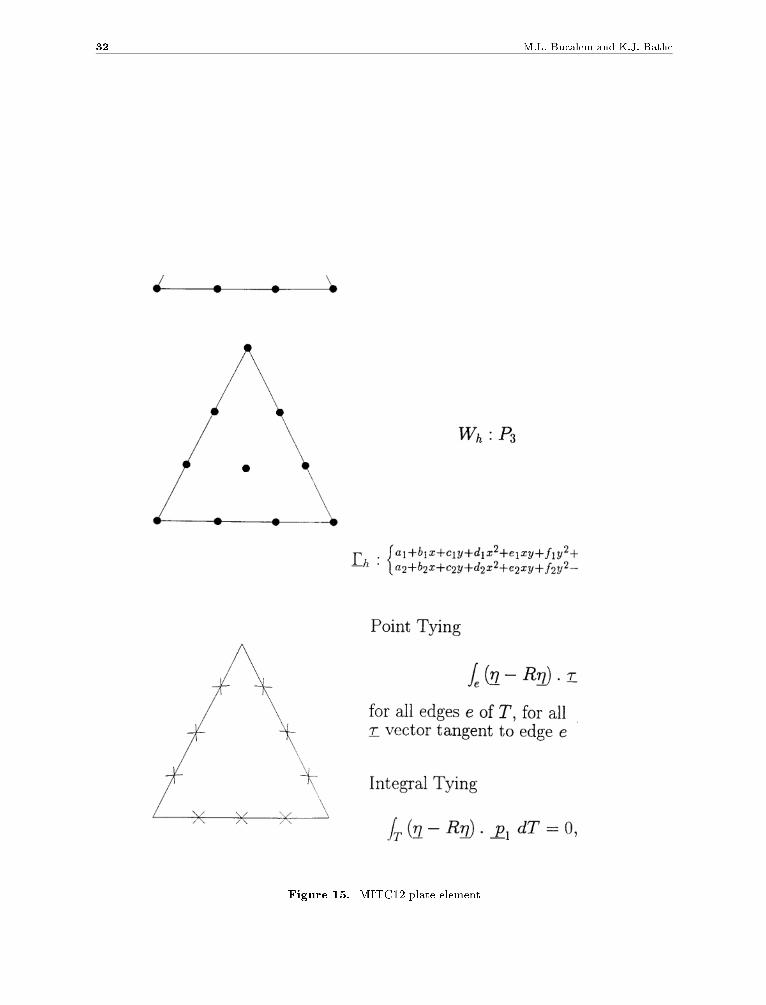
Figure 15. MITC12 plate element
Finite Element Analysis of Shell Structures 33
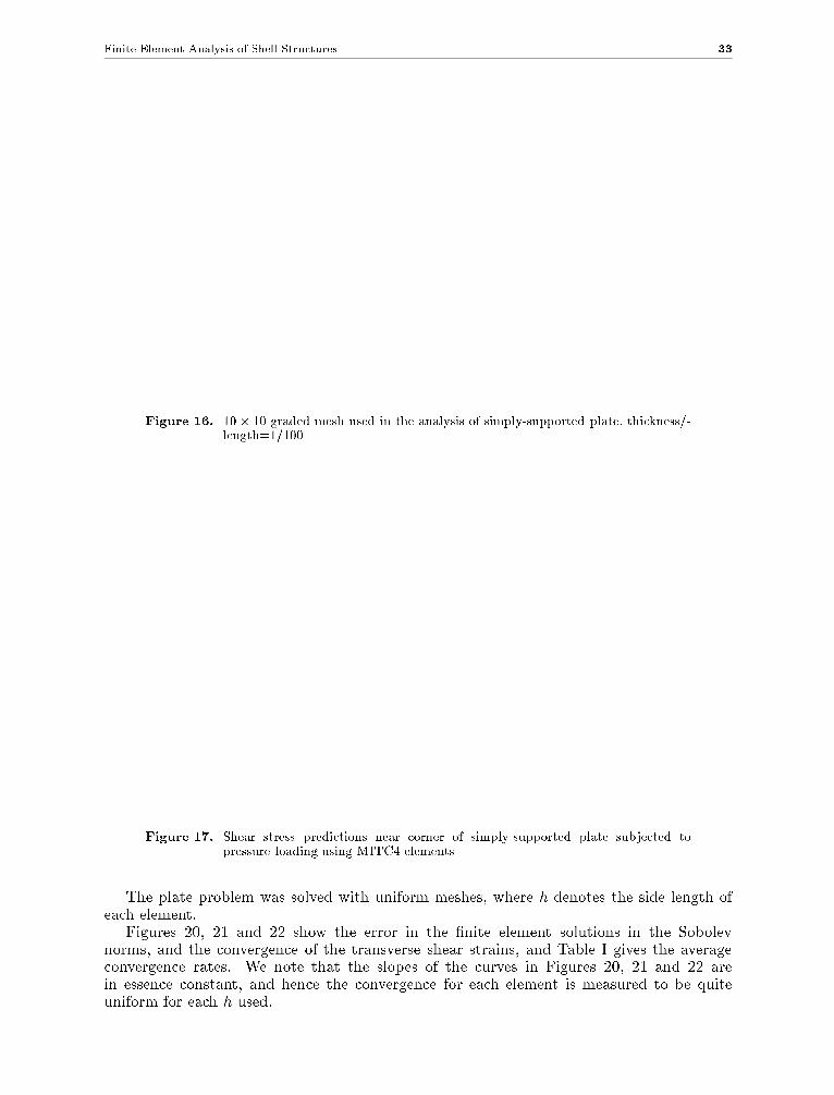
Figure 16. 10 � 10 graded mesh used in the analysis of simply-supported plate, thickness/-length=1=100
Figure 17. Shear stress predictions near corner of simply-supported plate subjected topressure loading using MITC4 elements
The plate problem was solved with uniform meshes, where h denotes the side length ofeach element.
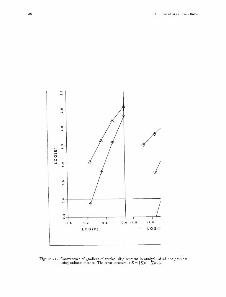
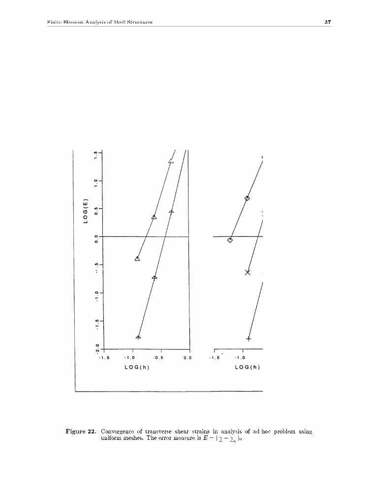
Figures 20, 21 and 22 show the error in the �nite element solutions in the Sobolevnorms, and the convergence of the transverse shear strains, and Table I gives the averageconvergence rates. We note that the slopes of the curves in Figures 20, 21 and 22 arein essence constant, and hence the convergence for each element is measured to be quiteuniform for each h used.

34 M.L. Bucalem and K.J. Bathe
Figure 18. Shear stress predictions near corner of simply-supported plate subjected topressure loading using MITC9 elements
Figure 19. Square plate used in the analysis of ad-hoc problem. The dashed line indicatethe subdivision used for triangular elements
Table 1 shows that the numerically obtained convergence rates are quite close to thetheoretical rates, and that the convergence of the transverse shear strain components issurprisingly good. The same study was performed with meshes that have been deliberateddistorted [25].
The distorted meshes resulted generally into a decrease of the convergence rates, but thisdecrease was not drastic when considering that rather highly distorted meshes were used,and when taking into account that each mesh contained rather large and small elements.

Finite Element Analysis of Shell Structures 35
Figure 20. Convergence of section rotations in analysis of ad-hoc problem using uniformmeshes. The error measure is E = k� � �
hk1
36 M.L. Bucalem and K.J. Bathe
Figure 21. Convergence of gradient of vertical displacement in analysis of ad-hoc problemusing uniform meshes. The error measure is E = krw �rwhk0
Finite Element Analysis of Shell Structures 37
Figure 22. Convergence of transverse shear strains in analysis of ad-hoc problem usinguniform meshes. The error measure is E = k �
hk0

38 M.L. Bucalem and K.J. Bathe
ELEMENT k� � �hk1 k� � �hk0 krw �rwhk0 kw � whk0 k � hk0
Theory Numerical Theory Numerical
MITC4 1.0 1.0 2.0 1.0 1.0 2.1 2.4
MITC9 2.0 1.8 2.7 2.0 2.0 3.0 3.2
MITC7 2.0 1.7 2.7 2.0 1.7 2.9 2.8
MITC12 3.0 2.7 3.7 3.0 2.7 3.8 3.9
MITC16 3.0 2.8 3.7 3.0 3.2 4.2 4.1
Table 1. Convergence rates obtained in analysis of ad-hoc problem using uniform meshes
Figure 23. Meshes used in analysis of circular plate, Young's modulus E = 2:1 � 106,Poisson's ratio � = 0:3, pressure p = 0:03072, diameter D = 20:0
4.2.34.2.3 Convergence in the analysis of a circular plateConvergence in the analysis of a circular plate
In this solution we consider a circular plate of thickness t and diameter D. The plate isloaded by a uniform pressure and is simply-supported or clamped along its edge.
Figure 23 gives the data of the problem considered and shows the �nite element meshesused. Note that the elements are geometrically distorted in a natural way in order to modelthe plate.

Finite Element Analysis of Shell Structures 39
Of particular interest in this analysis is the prediction of the transverse shear stresses.The analytical solution is rather simple (Figure 24) and there is no boundary layer. Figure 24shows the calculated stresses as obtained for the simply-supported plate using mesh A forthe MITC16 plate and shell elements and the usual 16-node displacement-based element.In this �gure we show the stresses calculated at those nodal points along line PO where twoelements meet. The stresses for an element at a nodal point have been calculated using forthat element
� = C bB u (68)
where � is the vector of the stresses, C is the stress-strain matrix, bB is the strain-displacement matrix of the element at the nodal point considered and u is the nodal pointdisplacement vector.
Figure 24. Mesh A shear stress predictions for analysis of simply supported circular plate,diameter/thickness = 100. The results not shown for the 16-node displacementbased shell element are actually outside the �gure
Hence there is no stress smoothing and at each nodal point where elements meet twovalues for each shear stress component are obtained.We note that the solution is veryaccurate using the MITC16 plate element with only three elements. On the other hand,the displacement-based element does not give an accurate transverse shear stress predictionunless a very �ne mesh is employed [25]. The MITC16 shell element is not as accurate asthe MITC16 plate element, as expected, but it provides good stress predictions consideringthat the mesh used is quite coarse.
Figure 25 presents the same type of shear stress results using the mesh B shown in Figure23 and the MITC9 plate and shell elements. A similar behavior as noted for the 16{nodeelements is encountered.
5. THE SPECIFICATION OF BOUNDARY CONDITIONS
The analysis of a structure requires the imposition of displacement/section rotation bound-ary conditions and force/moment boundary conditions (also referred to as essential andnatural boundary conditions, respectively [29]).

40 M.L. Bucalem and K.J. Bathe
Figure 25. Mesh B shear stress predictions for analysis of clamped circular plate, diame-ter/thickness = 100
As discussed in Section 3.2, the shell elements presented in this work have �ve natu-ral sti�ness degrees of freedom at a shell node, although when element assemblages areconsidered the use of six degrees of freedom at a shell node may be appropriate.
The objective in this section is to brie y discuss the imposition of plate and shellgeometric boundary conditions. Namely, there are some special considerations that needto be kept in mind when imposing the boundary conditions on the displacement-basedor mixed-interpolated elements, and we discuss these in the following by considering theanalysis of plates [29, 40, 41].
Consider the skew plate of side lengths L shown in Figure 26. The angle � is a variableso that with � = �
2we have a square plate. The thickness of the plate is h. The sides of
the plate can be �xed, simply-supported or free of support and the question we ask is howto impose these geometric boundary conditions.
The free support condition means, of course, that the displacement w and the rotations�n and �s are free along the edge.
The conditions of �xed and simply-supported edges, however, need special considerations.In Kirchho� plate theory, a simply-supported edge is modeled by the condition w = 0
and this means implicitly that also �s = 0. Namely, since @w
@s= �s, we have that if w = 0
along the edge, �s must be zero also. However, in the Reissner-Mindlin plate theory w and�s are independent variables and the usual \simple" support is appropriately modeled usingonly the condition w = 0. With this geometric condition, the transverse displacement iszero along the edge, but the section rotations corresponding to �s are not necessarily zero.
Therefore, in the �nite element solutions of plates using Reissner-Mindlin theory basedelements, the nodal transverse displacements should be set equal to zero at simply-supportededges, but the section rotations should usually be left free. These boundary conditions arereferred to as \soft-support" boundary conditions. Of course, it would be appropriate to alsoset the nodal rotations corresponding to �s equal to zero if the speci�c physical situation ofthe simple support is in this way more adequately modeled. This corresponds to the \hard-support" condition, and then restraining moments Mns are generated and the boundaryshear stresses are quite di�erent from those calculated when the soft-support condition isassumed.

Finite Element Analysis of Shell Structures 41
Figure 26. Plane view of plate; Tn is the shearing force
A most interesting phenomenon is that with the soft-support condition the boundaryshear stresses approach the Kirchho� solution through the development of a boundary layeras the thickness of the plate decreases.
Similar observations hold when a �xed edge is considered. Again, the choice of whetherto restrain the nodal rotations corresponding to �s must be decided depending on the actualphysical support to be modeled.
Figure 27 shows the analysis results reported in [40] for the solution of a simply-supportedsquare plate subjected to a uniform pressure, p. The plate was modeled using the 16-nodedisplacement-based element with the mesh given in Figure 27a. Figures 27b and 27c showresults obtained when the normal rotation �s is set to zero. We observe that the predictedshearing force is equal to the shearing force calculated by the Kirchho� plate theory whenthe twisting moment contribution is neglected. This twisting moment is resisted by themoment reaction Mns, for which the calculated values are close to the Kirchho� solution.We note that there is no boundary layer in the solution. Also, the corner reaction forces arezero and hence in this physical situation the plate does not have the tendency to rise at thecorner.
6. SAMPLE SOLUTIONS AND EVALUATION OF ELEMENTS
The analyses presented in this section have been chosen to illustrate the predictive capabili-ties of the MITC4, MITC8, MITC9 and MITC16 elements. As previously mentioned, theseelements are believed to be very e�ective general purpose shell elements.
Of course, these elements do not contain any spurious zero energy modes. The analyseswere conducted using the ADINA program, version 6.0 [42], modi�ed by the implementationof the MITC9 and MITC16 elements.

42 M.L. Bucalem and K.J. Bathe
(a) Finite element idealizations using 16-node displacement-based elements
(b) Shearing force distribution along AB assuming �s = 0
(c) Twisting moment distribution along AB assuming �s = 0
Figure 27. Analysis of simply-supported plate. \Hard" boundary conditions
Finite Element Analysis of Shell Structures 43
6.1 Patch Test
The patch test has been widely used as a test for element convergence, despite its limitationsfor mixed formulations. We use the test here to assess the sensitivity of our elements togeometric distortions.
The test we use has been reported earlier (e.g., [21]); namely a patch of elements (with notall of the elements of rectangular shape) is subjected to the minimum displacement/rotationboundary conditions to restrain the structure from rigid body motion. The boundary of thepatch is subjected to the tractions that correspond to the constant stress states.
The behavior of the elements is considered satisfactory if the constant stress state isrepresented by the �nite element model.
The above patch test is a standard procedure to test for constant stress states. Ofcourse, we may also test whether higher-order stress variations can be properly representedby the patch. This is achieved by subjecting the patch of elements to the body forces andboundary tractions that correspond (in the plate theory solution) to the stress variations tobe predicted by the patch. Then the �nite element stress predictions can be compared withthe desired higher-order stress variations.
The MITC4, MITC8, MITC9 and MITC16 elements can represent the constant stressstates as long as the element sides are straight.
6.2 Analysis of a Clamped Square Plate
Figure 28 shows the square plate considered in this analysis. Note that the thickness tolength ratio is 1000. Hence, we consider a thin plate and models with elements that shearlock would give highly inaccurate results.
Figure 28 also shows a typical 2 � 2 mesh used and in Figure 29 two distorted elementmesh layouts are shown. The meshes distort-1 and distort-2 would of course hardly be usedin practice, but have merely been selected here to test the predictive capabilities of theelements.
Tables 2 and 3 list the results obtained in the plate analyses using the di�erent elements.The results in particular indicate the high predictive capability of the MITC8 element.
6.3 Analysis of a Skew Plate
The Morley skew plate problem has also been used as a test problem for plate/shell elements.The data of the problem is presented in Figure 30. Generally, the results reported refer tothe vertical displacement at the center of the plate i.e., at point E, and these are presentedfor the MITC plate and shell elements in [38]. Here we show selected results of a modalanalysis. In Figures 31 and 32 we show the \Sussman-Bathe" band plots [44] for the verticaldisplacement component of the eigenvector and for the average in-plane modal stresses at thetop surface of the plate. The results are shown for mode 2 and for the MITC4 and MITC8elements. A uniform mesh of (16 � 16) MITC4 elements and a uniform mesh of (8 � 8)MITC8 elements are used. We observe that the displacement results obtained are quitesimilar for both types of elements. However, the accuracy of the modal stress predictionsare quite di�erent for the elements used. Considering the MITC8 element results we canidentify clearly continuous stress bands across element boundaries indicating the adequacyof this mesh for these modal stress predictions whereas in the MITC4 element results wecannot identify a distinguishable stress band pattern. These sample results show once morethe importance of using higher-order elements when a stress response is sought.

44 M.L. Bucalem and K.J. Bathe
Figure 28. Analysis of a clamped thin square plate. A 2� 2 mesh model
(a) Distort{1
(b) Distort{2
Figure 29. Arti�cially distorted meshes in the analysis of a clamped plate. One quarter ofthe mesh shown

Finite Element Analysis of Shell Structures 45
Table 2. Performance of the elements in analysis of plate. Uniform pressure loading
Table 3. Performance of the elements in analysis of plate. Concentrated load
6.4 Analysis of a Curve Cantilever
We consider the curved cantilever problem described in Figure 33. In Table 4 we showthe results obtained for various meshes using the 16-node displacement-based element andthe MITC16 element. The ratio between the �nite element and the analytical predictionsfor the tip rotation, at point A, are shown for several values of thickness. We notice thatthe predictions are excellent for most discretizations even for extremely thin situations(h=R = 1=105). However, for the two element model when the side that is common to the

46 M.L. Bucalem and K.J. Bathe
Figure 30. Morley skew plate problem
Figure 31. Modal results for the Morley skew plate using a (16 � 16) uniform mesh ofMITC4 elements. The symbol AVG stands for the average in plane stress givenby (�xx + �yy)=2 and ZEIGEN for the Z component of the mode eigenvector

Finite Element Analysis of Shell Structures 47
Figure 32. Modal results for the Morley skew plate using a (8� 8) uniform mesh of MITC8elements. The symbol AVG stands for the average in plane stress given by(�xx + �yy)=2 and ZEIGEN for the Z component of the mode eigenvector
two elements, and is parallel to the axis of the cylindrical surface that describes the curvedcantilever, is skewed the results signi�cantly deteriorate for the 16-node displacement-basedelement displaying a locking behavior. This type of behavior was theoretically predicted byPitk�aranta [26].
In Table 5 we show analogous results for the MITC8 and the MITC9 elements. Using theMITC8 element, which is a good element in general, the results also deteriore signi�cantlyfor the above case. We notice that the MITC9 element does not display such a behavior.
In the results presented we used � = 0:0 but the the same kind of solution accuracy isdisplayed when � = 0:3.

48 M.L. Bucalem and K.J. Bathe
Figure 33. Analysis of a curved cantilever
Table 4. Summary of results for the curved cantilever problem using 16-node elements. PointA always coincides with an element node

Finite Element Analysis of Shell Structures 49
Table 5. Summary of results for the curved cantilever problem using 8- and 9-node mixed-interpolated elements. Point A always coincides with an element node
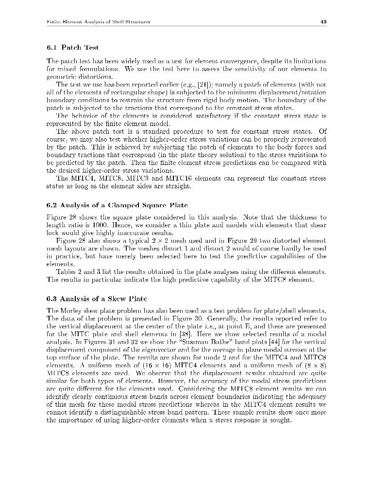
6.5 Analysis of a Pinched Cylinder
The pinched-cylinder problem has been widely used to test shell elements. The physicalproblem is presented in Figure 34. Due to symmetry conditions only one octant of thecylinder needs to be considered.
Figure 35 shows a typical mesh used in this solution (for 1/8th of the cylinder). This�gure also shows that 6 nodal degrees of freedom have been speci�ed at the symmetry linesand otherwise 5 nodal degrees of freedom have been employed. This allocation of nodal pointdegrees of freedom is eÆcient because then symmetry conditions can be easily imposed (Asimilar nodal degree of freedom allocation was used for the analyses discussed below). Noattempt was made to identify for the analysis an optimal mesh, but a graded mesh is usedbecause the stresses vary rapidly as the concentrated load is approached.
Table 6 gives the solution results. Note that because of the stress singularity under theconcentrated load, this load should be thought of as being distributed over a \small" areaif a very �ne mesh were to be used [29].
We also performed a study using uniform meshes and the results are shown in Figure 36.The performance of the MITC elements of various orders and also the performance ofelements that have been proposed by other authors are shown. In the comparison weused as the index of mesh re�nement the number of nodes per side of the region discretized.We notice the excellent performance of the higher{order MITC elements. The results arenormalized with respect to the analytical solution for this problem reported by Lindberg et.
al. [43].
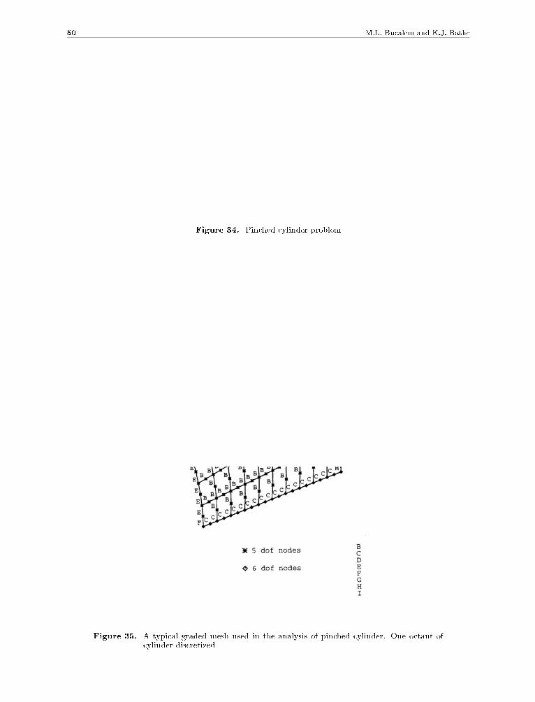
50 M.L. Bucalem and K.J. Bathe
Figure 34. Pinched cylinder problem
Figure 35. A typical graded mesh used in the analysis of pinched cylinder. One octant ofcylinder discretized
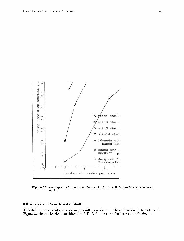
Finite Element Analysis of Shell Structures 51
Figure 36. Convergence of various shell elements in pinched cylinder problem using uniformmeshes
6.6 Analysis of Scordelis-Lo Shell
This shell problem is also a problem generally considered in the evaluation of shell elements.Figure 37 shows the shell considered and Table 7 lists the solution results obtained.

52 M.L. Bucalem and K.J. Bathe
Table 6. Performance of elements in analysis of pinched cylinder
Figure 37. Scordelis-Lo problem
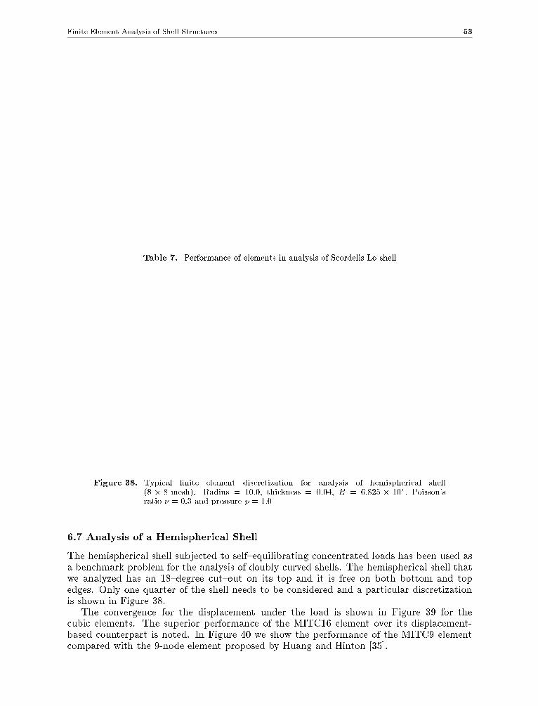
Finite Element Analysis of Shell Structures 53
Table 7. Performance of elements in analysis of Scordelis-Lo shell
Figure 38. Typical �nite element discretization for analysis of hemispherical shell(8 � 8 mesh). Radius = 10:0, thickness = 0:04, E = 6:825 � 107, Poisson'sratio � = 0:3 and pressure p = 1:0
6.7 Analysis of a Hemispherical Shell
The hemispherical shell subjected to self{equilibrating concentrated loads has been used asa benchmark problem for the analysis of doubly curved shells. The hemispherical shell thatwe analyzed has an 18{degree cut{out on its top and it is free on both bottom and topedges. Only one quarter of the shell needs to be considered and a particular discretizationis shown in Figure 38.
The convergence for the displacement under the load is shown in Figure 39 for thecubic elements. The superior performance of the MITC16 element over its displacement-based counterpart is noted. In Figure 40 we show the performance of the MITC9 elementcompared with the 9-node element proposed by Huang and Hinton [35].

54 M.L. Bucalem and K.J. Bathe
Figure 39. Convergence in analysis of hemispherical shell, cubic elements

Finite Element Analysis of Shell Structures 55
Figure 40. Convergence in analysis of hemispherical shell, 9-node elements
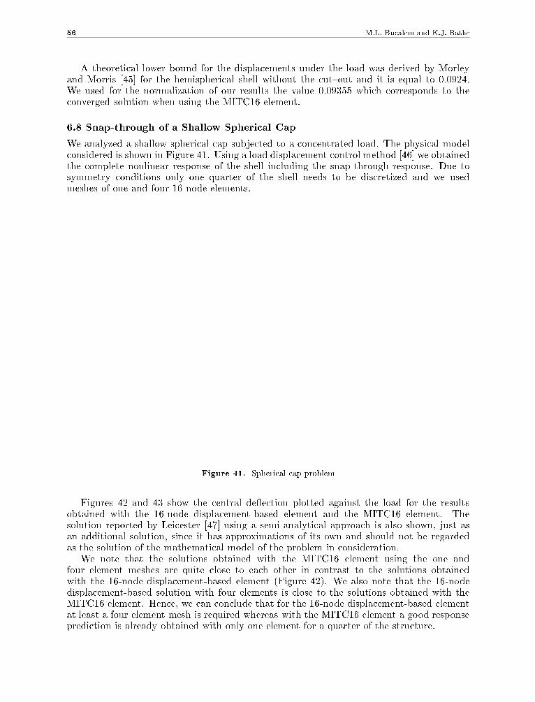
56 M.L. Bucalem and K.J. Bathe
A theoretical lower bound for the displacements under the load was derived by Morleyand Morris [45] for the hemispherical shell without the cut{out and it is equal to 0.0924.We used for the normalization of our results the value 0.09355 which corresponds to theconverged solution when using the MITC16 element.
6.8 Snap-through of a Shallow Spherical Cap
We analyzed a shallow spherical cap subjected to a concentrated load. The physical modelconsidered is shown in Figure 41. Using a load displacement control method [46] we obtainedthe complete nonlinear response of the shell including the snap-through response. Due tosymmetry conditions only one quarter of the shell needs to be discretized and we usedmeshes of one and four 16-node elements.
Figure 41. Spherical cap problem
Figures 42 and 43 show the central de ection plotted against the load for the resultsobtained with the 16-node displacement-based element and the MITC16 element. Thesolution reported by Leicester [47] using a semi-analytical approach is also shown, just asan additional solution, since it has approximations of its own and should not be regardedas the solution of the mathematical model of the problem in consideration.
We note that the solutions obtained with the MITC16 element using the one andfour element meshes are quite close to each other in contrast to the solutions obtainedwith the 16-node displacement-based element (Figure 42). We also note that the 16-nodedisplacement-based solution with four elements is close to the solutions obtained with theMITC16 element. Hence, we can conclude that for the 16-node displacement-based elementat least a four element mesh is required whereas with the MITC16 element a good responseprediction is already obtained with only one element for a quarter of the structure.
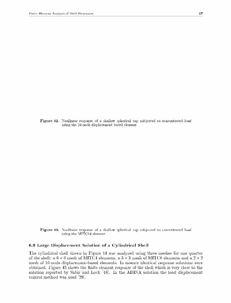
Finite Element Analysis of Shell Structures 57
Figure 42. Nonlinear response of a shallow spherical cap subjected to concentrated loadusing the 16-node displacement based element
Figure 43. Nonlinear response of a shallow spherical cap subjected to concentrated loadusing the MITC16 element
6.9 Large Displacement Solution of a Cylindrical Shell
The cylindrical shell shown in Figure 44 was analyzed using three meshes for one quarterof the shell: a 6� 6 mesh of MITC4 elements, a 3� 3 mesh of MITC8 elements and a 2� 2mesh of 16-node displacement-based elements. In essence identical response solutions wereobtained. Figure 45 shows the �nite element response of the shell which is very close to thesolution reported by Sabir and Lock [48]. In the ADINA solution the load displacementcontrol method was used [29].

58 M.L. Bucalem and K.J. Bathe
Figure 44. Large displacement analysis of shallow cylindrical shell
Figure 45. Finite element displacement solutions in analysis of cylindrical shell
7. CONCLUDING REMARKS
The objective in this paper was to summarize some state-of-the-art capabilities for shellstructural analysis. The formulation of recommended shell elements and numerical experi-ences were presented.
The shell analysis capabilities currently available are general and e�ective and generalproblems can be solved with con�dence. As for future developments, the use of the mixedinterpolation for element formulations has signi�cant further potential and is expected toyield additional valuable elements.

Finite Element Analysis of Shell Structures 59
REFERENCES
1 Noor, A. et al. (eds.) (1989), \Analytical and Computational Models of Shells", ASME Special
Publication, CED{3.
2 Bathe, K.J. and Dvorkin, E. (1986), \A Formulation of General Shell Elements | the Use ofMixed Interpolation of Tensorial Components", International Journal for Numerical Methods in
Engineering, 22, pp. 697{722.
3 Love, A.E.H. (1888), \The Small Free Vibrations and Deformation of a Thin Elastic Shells", Phil.Trans. Roy. Soc. London, (Ser. A 179), pp. 491{546.
4 Koiter, W.T. (1959), \A Consistent First Approximation in General Theory of Thin ElasticShells", In Proc. IUTAM Symposium on the Theory of Thin Elastic Shells, Delft, pp. 12{33.
5 Sanders, J.L. Jr. (1959), \An Improved First Approximation Theory for Thin Shells", Tech.Report R-24, NASA.
6 Kardestuncer, H. (ed.) (1987), \Finite Element Handbook", MacGraw-Hill.
7 Ahmad, S., Irons, B.M. and Zienkiewicz, O.C. (1970), \Analysis of Thick and Thin Shell Struc-tures by Curved Finite Elements", International Journal for Numerical Methods in Engineering,2, pp. 419{451.
8 Ramm. E. (1977), \A Plate/Shell Element for Large De ections and Rotations", In Bathe, K.J.(ed.), Formulations and Computational Algorithms in Finite Element Analysis, M.I.T. Press.
9 Bathe, K.J. and Bolourchi, S. (1979), \A Geometric and Material Nonlinear Plate and ShellElement", Computers & Structures, 11, 23{48.
10 Zienkiewicz, O.C., Taylor, R.L. and Too, J.M. (1971), \Reduced Integration Techniques in Gen-eral Analysis of Plates and Shells", International Journal for Numerical Methods in Engineering,3, pp. 275{290.
11 O~nate, E., Hinton, E. and Glover, N. (1978), \Techniques for Improving the Performance ofthe Ahmad Shell Elements", Proc. Int. Conf. on Applied Numerical Modelling, Pentech Press,Madrid, pp. 30{53.
12 Hughes, T.J.R., Cohen, M. and Haroun, M. (1978), \Reduced and Selective Integration Tech-niques in the Finite Element Analysis of Plates", Nuclear Engineering Design, 46, pp. 203{222.
13 Malkus, D.S. and Hughes, T.J.R. (1978), \ Mixed Finite Element Methods-Reduced and SelectiveIntegration Techniques: A Uni�cation of Concepts", Computer Methods in Applied Mechanics
and Engineering, 15, pp. 63{81.
14 Bercovier, M. (1978), \Perturbation of a Mixed Variational Problems, Applications to MixedFinite Element Methods", R.A.I.R.O. Anal. Numer., 12, pp. 211{236.
15 Belytschko, T., Liu, W.K., Ong, S.J. and Lam, D. (1985), \Implementation and Application ofa 9-node Lagrange Shell Element with Spurious Mode Control", Computers & Structures, 20,(1-3), pp. 121{128.
16 Belytschko, T., Ong, S.J. and Liu, W.K. (1985), \A Consistent Control of Spurious SingularModes in the 9{Node Lagrangian Element for the Laplace and Mindlin Plate Equations" Com-
puter Methods in Applied Mechanics and Engineering, 44, pp. 269{295.
17 Bathe, K.J. and Brezzi, F. (1985), \On the Convergence of a Four-Node Plate Bending ElementBased on Mindlin/Reissner Plate Theory and a Mixed Interpolation", In Whiteman, J.R. (ed.),Proceedings of the Conference on Mathematics of Finite Elements and Applications V, AcademicPress, pp. 491{503.
60 M.L. Bucalem and K.J. Bathe
18 Bathe, K.J. and Brezzi, F. (1987), \A Simpli�ed Analysis of Two{Plate Bending Elements {the MITC4 and MITC9 Elements", In Pande, G.N. and Middleton, J. (eds.), Proceedings of
the International Conference on Numerical Methods in Engineering (NUMETA 87), UniversityCollege of Swansea, Wales, p. D46.
19 Brezzi, F., Bathe, K.J. and Fortin, M. (1989), \Mixed-Interpolated Elements for Reissner-MindlinPlates", International Journal for Numerical Methods in Engineering, 28, pp. 1787{1801.
20 Brezzi, F., Fortin, M. and Stenberg, R. (1991), \Error Analysis of Mixed{Interpolated Elementsfor Reissner{Mindlin Plates", Mathematical Models and Methods in Applied Sciences, 1, pp.125{151.
21 Dvorkin, E. and Bathe, K.J. (1984), \A Continuum Mechanics Based Four-Node Shell Elementfor General Nonlinear Analysis", Engineering Computations, 1, pp. 77{88.
22 Bathe, K.J. and Dvorkin, E. (1985), \A Four-Node Plate Bending Element Based on Mindlin{Reissner Plate Theory and a Mixed Interpolation", International Journal for Numerical Methods
in Engineering, 21, pp. 367{383.
23 Bathe, K.J., Cho, S.W., Bucalem, M.L. and Brezzi, F. (1989), \On Our MITC Plate Bend-ing/Shell Elements", In Noor, A. et al. (eds.), Analytical and Computational Models of Shells,CED{3, ASME Special Publication, pp. 261{278.
24 Bathe, K.J., Brezzi, F. and Cho, S.W. (1989), \The MITC7 and MITC9 Plate Bending Elements",Computers & Structures, 32, (3/4), pp. 797{814.
25 Bathe, K.J., Bucalem, M.L. and Brezzi, F. (1990), \Displacement and Stress Convergence of OurMITC Plate Bending Elements", Engineering Computations, 7, 4, pp. 291{302.
26 Pitk�aranta, J. (1991), \The Problem of Membrane Locking in Finite Element Analysis of Cylin-drical Shells", Report, Helsinki University of Technology, Otakaari 1, SF-02150 Espoo, Finland.
27 Hughes, T.J.R. and Tezduyar, T.E. (1981), \Finite Elements Based upon Mindlin Plate Theorywith Particular Reference to the Four-Node Bilinear Isoparametric Element", Journal of AppliedMechanics, Transactions of ASME, 48, pp. 587{596.
28 MacNeal, R.H., (1982), \Derivation of Element Sti�ness Matrices by Assumed Strain Distribu-tions", Nuclear Engineering Design, 70, pp. 3{12.
29 Bathe, K.J. (1996), \Finite Element Procedures", Prentice Hall, Inc., Englewood Cli�s.
30 Schweizerhof, K. and Ramm, E. (1984), \Displacement Dependent Pressure Loads in NonlinearFinite Element Analysis", Computers & Structures, 28, pp. 1099-1114.
31 Argyris, J. (1982), \An Excursion with Large Rotations", Computer Methods in Applied Mechan-
ics and Engineering, 32, pp. 85-155.
32 Bathe, K.J. (1986), \Finite Elements in CAD and ADINA", Journal of Nuclear Engineering andDesign, 98, pp. 57{67.
33 Bathe, K.J. and Ho, L. (1981), \Finite Elements in CAD and ADINA", Nonlinear Finite ElementAnalysis in Structural Mechanics, Wunderlich, W. et al. (eds.), Springer Verlag, Berlin.
34 Hughes, T.J.R., Taylor, R.L. and Kanoknukulchai (1977), \A Simple and EÆcient Finite Elementfor Plate Bending", International Journal for Numerical Methods in Engineering, 11, pp. 1529-1543.
35 Huang, H.C. and Hinton, E. (1986), \A New Nine{Node Degenerated Shell Element with En-hanced Membrane and Shear Interpolation", International Journal for Numerical Methods in
Engineering, 22, pp. 73{92.
Finite Element Analysis of Shell Structures 61
36 Park, K.C. and Stanley, G.M. (1986), \A curved C0 Shell Element Based on Assumed Natural-Coordinate Strains", Journal of Applied Mechanics, Transactions of ASME, 53, pp. 278{290.
37 Jang, J. and Pinsky, P.M. (1987), \An Assumed Covariant Strain Based 9-Node Shell Element",International Journal for Numerical Methods in Engineering, 24, pp. 2389{2411.
38 Bucalem, M.L. and Bathe, K.J. (1993), \Higher-Order MITC General Shell Elements", Interna-tional Journal for Numerical Methods in Engineering, 36, pp. 3729{3754.
39 Sussman, T. and Bathe, K.J. (1987), \A Finite Element Formulation for Nonlinear IncompressibleElastic and Inelastic Analysis", Computers & Structures, 26, pp. 357{409.
40 H�aggblad, B. and Bathe, K.J. (1990), \Speci�cations of Boundary Conditions for Reissner{Mindlin Plate Bending Finite Elements", International Journal for Numerical Methods in Engi-
neering, 30, pp. 981{1011.
41 Arnold, D.N. and Falk, R.S. (1989), \Edge E�ects in Reissner{Mindlin Plate Theory", In Noor, A.et al., (eds.) Analytical and Computational Models of Shells, CED{3, ASME Special Publication.
42 ADINA R&D (1990), \ADINA{A Finite Element Program for Automatic Dynamic IncrementalNonlinear Analysis", Report 90{1, ADINA R&D, Watertown, MA.
43 Lindberg, G.M., Olson, M.D. and Cowper, E.R. (1969), \New Developments in the Finite ElementAnalysis of Shells", National Research Council of Canada, Quarterly Bulletin of the Division of
Mechanical Engineering and the National Aeronautical Establishment, 4, pp. 1{38.
44 Sussman, T. and Bathe, K.J. (1986), \Studies of Finite Element Procedures. Stress Band Plotsand the Evaluation of Finite Element Meshes", Engineering Computations, 3, pp. 178{191.
45 Morley, L.S.D. and Morris, A.J. (1978), \Con ict Between Finite Elements and Shell Theory",Technical report, Royal Aicraft Establishment Report, London.
46 Bathe, K.J. and Dvorkin, E.N. (1983), \On the Automatic Solution of Nonlinear Finite ElementEquations", Computers & Structures, 17, 5-6, pp. 871{879.
47 Leicester, R.H. (1968), \Finite Deformations of Shallow Shells", In Proceedings of American
Society of Civil Engineers, 94, (EM6), pp. 1409{1423.
48 Sabir, A.B. and Lock, A.C. (1973), \The Application of Finite Elements in the Large De ectionGeometrically Nonlinear Behavior of Cylindrical Shells", In Brebbia, A. and Totteham, H. (eds.),Variational Methods in Engineering, pp. 7/66{67/75, Southampton University Press.
49 Chapelle, D. and Bathe, K.J. (1993), \The Inf-Sup Test", Computer and Structures, 47, pp.537{545.
Please address your comments or questions on this paper to:
International Center for Numerical Methods in EngineeringEdi�cio C-1, Campus Norte UPCGran Capit�an s/n08034 Barcelona, SpainPhone: 34-3-4016035; Fax: 34-3-4016517


