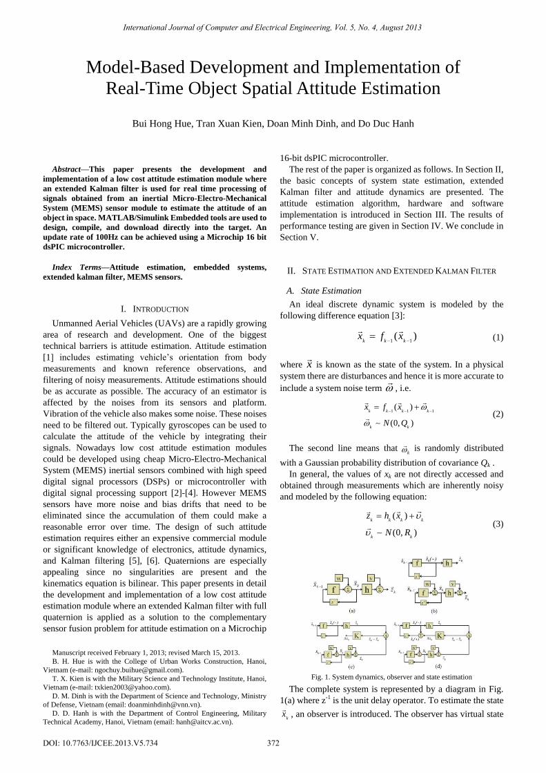
Abstract—This paper presents the development and

implementation of a low cost attitude estimation module where

an extended Kalman filter is used for real time processing of

signals obtained from an inertial Micro-Electro-Mechanical

System (MEMS) sensor module to estimate the attitude of an

object in space. MATLAB/Simulink Embedded tools are used to

design, compile, and download directly into the target. An

update rate of 100Hz can be achieved using a Microchip 16 bit

dsPIC microcontroller.

Index Terms—Attitude estimation, embedded systems,

extended kalman filter, MEMS sensors.

I. INTRODUCTION

Unmanned Aerial Vehicles (UAVs) are a rapidly growing

area of research and development. One of the biggest

technical barriers is attitude estimation. Attitude estimation

[1] includes estimating vehicle’s orientation from body

measurements and known reference observations, and

filtering of noisy measurements. Attitude estimations should

be as accurate as possible. The accuracy of an estimator is

affected by the noises from its sensors and platform.

Vibration of the vehicle also makes some noise. These noises

need to be filtered out. Typically gyroscopes can be used to

calculate the attitude of the vehicle by integrating their

signals. Nowadays low cost attitude estimation modules

could be developed using cheap Micro-Electro-Mechanical

System (MEMS) inertial sensors combined with high speed

digital signal processors (DSPs) or microcontroller with

digital signal processing support [2]-[4]. However MEMS

sensors have more noise and bias drifts that need to be

eliminated since the accumulation of them could make a

reasonable error over time. The design of such attitude

estimation requires either an expensive commercial module

or significant knowledge of electronics, attitude dynamics,

and Kalman filtering [5], [6]. Quaternions are especially

appealing since no singularities are present and the

kinematics equation is bilinear. This paper presents in detail

the development and implementation of a low cost attitude

estimation module where an extended Kalman filter with full

quaternion is applied as a solution to the complementary

sensor fusion problem for attitude estimation on a Microchip

Manuscript received February 1, 2013; revised March 15, 2013.

B. H. Hue is with the College of Urban Works Construction, Hanoi,

Vietnam (e-mail: ngochuy.buihue@gmail.com).

T. X. Kien is with the Military Science and Technology Institute, Hanoi,

Vietnam (e-mail: txkien2003@yahoo.com).

D. M. Dinh is with the Department of Science and Technology, Ministry

of Defense, Vietnam (email: doanminhdinh@vnn.vn).

D. D. Hanh is with the Department of Control Engineering, Military

Technical Academy, Hanoi, Vietnam (email: hanh@aitcv.ac.vn).

16-bit dsPIC microcontroller.

The rest of the paper is organized as follows. In Section II,

the basic concepts of system state estimation, extended

Kalman filter and attitude dynamics are presented. The

attitude estimation algorithm, hardware and software

implementation is introduced in Section III. The results of

performance testing are given in Section IV. We conclude in

Section V.

II. STATE ESTIMATION AND EXTENDED KALMAN FILTER

A. State Estimation

An ideal discrete dynamic system is modeled by the

following difference equation [3]:

1 1( )

k k kx f x

(1)

where x

is known as the state of the system. In a physical

system there are disturbances and hence it is more accurate to

include a system noise term

, i.e.

1 1 1( )

(0, )

k k k k

k k

x f x

N Q

(2)

The second line means that k

is randomly distributed

with a Gaussian probability distribution of covariance Qk .

In general, the values of xk are not directly accessed and

obtained through measurements which are inherently noisy

and modeled by the following equation:

( )

(0, )

k k k k

k k

z h x

N R

(3)

Fig. 1. System dynamics, observer and state estimation

The complete system is represented by a diagram in Fig.

1(a) where z-1 is the unit delay operator. To estimate the state

kx

, an observer is introduced. The observer has virtual state

Model-Based Development and Implementation of

Real-Time Object Spatial Attitude Estimation

Bui Hong Hue, Tran Xuan Kien, Doan Minh Dinh, and Do Duc Hanh

372

International Journal of Computer and Electrical Engineering, Vol. 5, No. 4, August 2013

DOI: 10.7763/IJCEE.2013.V5.734

ˆk

x , virtual measurements ˆkz , and obeys the same equations

as the real system but without noises, i.e.

1 1ˆ ˆ( )

ˆˆ ( )

k k k

k k k

x f x

z h x

(4)

The observer is assumed to run in parallel with the real

system (see Fig. 1(b)). Because of the system noise

, the a

priori propagated state ˆ ( )kx differs from the true state kx

and virtual measurement ˆkz does not agree with the actual

measurement kz

. Feedback gain Kk is introduced to estimate

the state error ˆ ˆk k kx x x

based on the measurement error

ˆk kz z

(see Fig. 1(c)). Finally, this error is used to correct

the observer's state, forming the a posteriori corrected state

ˆ ( )kx (see Fig. 1(d)).

B. Extended Kalman Filter

The expectation value of the state error ˆkx is known as

the covariance of the states expressed by the following

equation:

ˆ ˆ([ ][ ] )T

k k k k kP x x x x

(5)

An optimal feedback gain Kk can be derived by minimizing

Pk. For linear systems this is known as the Kalman filter and

was first presented in 1960 by Kalman [6]. The estimated

state and covariance are propagated at every time step, but in

many systems measurements are only sporadically available.

In this case the state covariance grows for many time steps as

the estimated state diverges from the true state. When a

measurement becomes available, the feedback gain K is

calculated, the state is corrected, and the state covariance is

updated (reduced) accordingly.

The Kalman filter has been applied to nonlinear systems in

many different ways. One of the most straightforward

techniques is to linearize the system dynamics and the

measurement function around the expected state ( )kx

, and

then apply the Kalman filter as normal. This is known as

extended Kalman filtering and the implementation equations

(borrowed from [5]) are presented in Table 1.

TABLE I: EXTENDED KALMAN FILTER IMPLEMENTATION EQUATIONS

System

dynamics

1 1 1( )k k k kx f x

(6.1)

(0, )k kN Q

(6.2)

Measurement ( )k k k kz h x v

(6.3)

(0, )k kv N R

(6.4)

Covariance ˆ ˆ([ ][ ] )T

k k k k kP x x x x

(6.5)

State

propagation

1 1ˆ ˆ( ) ( ( ))k k kx x (6.6)

Dynamics

linearization

1

11

ˆ ( )k

kk

x x

f

x

(6.7)

Predicted

measurement ˆ ( )k k kz h x

(6.8)

Measurement

linearization

ˆ ( )k

kk

x x

hH

x

(6.9)

State covariance

propagation

1 1 1 1( ) ( ) T

k k k k kP P Q (6.10)

Feedback gain ( ) ( )T T

k k k k k k kK P H H P H R (6.11)

State update ˆ ˆ ˆ( ) ( ) ( )k k k k kx x K z z (6.12)

State covariance

update ( ) (1 ) ( )k k k kP K H P (6.13)

Extended Kalman filter allows to dynamically estimate

attitude and drifting gyro biases, as long as they are modeled

as states in our dynamical system. Next the three-dimensional

attitude dynamics and measurement equations will be

derived.

C. Attitude Dynamics

Suppose there is a rigid body with the body coordinate

system OXYZ and let O0X0Y0Z0 be a reference (e.g. earth)

coordinate system (Fig. 2). Translate the origin of the

reference coordinate system to the origin of the body

coordinate system (keeping the directions of the axes O0X0,

O0Y0 and O0Z0 unchanged). The angles representing the

relationship between these two coordinate systems are called

orientation angles (attitude Euler angles) including yaw angle

ψ, pitch angle θ and roll angle φ.

Fig. 2. Rigid body coordinate system and reference coordinate system. 1 –

The horizontal plane; 2 – The object symetry plane; 3 – The vertical plane

containing the longitudinal axis; 4 - The vertical plane containing OZ axis.

From orientation angles, direction cosine matrix (DCM)

between two coordinate systems is calculated as follows [3]:

( , , )

sin sin

sin sin sin sin sin cos sin

sin sin sin s sin sin sin sin cos

b e

b e

b e

u u

v T v

w w

cos cos cos

T cos cos cos cos cos

cos co cos cos

(7)

where (ue; ve;we) is a vector in the reference frame, (ub; vb;wb)

is the vector in the rigid body frame (X;Y; Z).

It turns out that the Euler angle dynamics can be derived by

inspection alone. Because the body rotation rates

x y z are defined as instantaneous rotation rates

about the OX, OY, and OZ axes respectively, it can be

observed that is a rotation about the OX axis. θ is a rotation

about an intermediate axis, so to project onto the body

frame it must be rotated using the rotation. Likewise,

373

International Journal of Computer and Electrical Engineering, Vol. 5, No. 4, August 2013

must be rotated about first θ, and then , i.e.

0 0

0 0

0 0

x

y

z

T T T

(8)

From (8) and (7) we obtain:

1 sin( ) tan( ) cos( ) tan( )

0 cos( ) sin( )

0 sin( )sec( ) cos( )sec( )

x

y

z

(9)

Quaternions are hyper-complex numbers of rank 4. A

quaternion q can be expressed as:

0 1 2 3q q iq jq kq

Then the DCM is a function of q:

2 2

0 1 1 2 0 3 1 3 0 2

2 2

1 2 0 3 0 2 2 3 0 1

2 2

1 3 0 2 2 3 0 1 0 3

( )

2 2 1 2 2 2 2

2 2 2 2 1 2 2

2 2 2 2 2 2 1

b e

b e

b e

u u

v T q v

w w

q q q q q q q q q q

T q q q q q q q q q q

q q q q q q q q q q

(10)

III. IMPLEMENTATION

A. Implementation Equations

The attitude estimation module is developed using an

extended Kalman filter with the full quaternion [q0 q1 q2

q3]T. The state is 0 1 2 3 1 2 3 1 2 3

Tx q q q q b b b

, where bi are

the gyro biases. The implementation follows equations

summarized in Table 1 and it is necessary to derive the state

transfer functions f and Ф, the measurement functions h and

H, and the noise covariances Q and R.

1) State transfer functions

Rotation angular velocities and drifts of the gyro are

assumed to be stochastic processes, i.e.

1 , 1

1 , 1

k k k

k k b kb b

(11)

State transfer function f is derived from the above equation

and equation 6.1. From equation 6.7, Φ is obtained by taking

partial derivatives of f.

The state 1kx

is represented as follows:

31 2

31 2

32

. . . .cos sin sin sin

2 2 2 2

. . . .sin cos sin sin

2 2 2 2

. . .sin sin cos

2 2 2

t t t t

t t t t

t t t1

3 2 1

.sin

2

. . . .sin sin sin cos

2 2 2 2

t

t t t t

2) Measurement functions

Measurement of gravity and inertial acceleration in the

body frame is expressed by:

accel

x

z T y

z g

(12)

Most efficient computation is with aacurate tracking

estimation, i.e. q q

, and then subtracting the inertial

accelerations measured by GPS we obtain:

ˆ

0

0accel q q q

x x

z T y T y T

z g z g

(13)

After coordinate transformation we obtain:

2 21 3 0 20 1 1 2 0 3 1 3 0 2

2 2

1 2 0 3 0 2 2 3 0 1 2 3 0 1

2 2 2 21 3 0 2 2 3 0 1 0 3 0 3

2 ( )2 2 1 2 2 2 2 0

2 2 2 2 1 2 2 0 2 ( )

2 2 2 2 2 2 1 (2 2 1)

aceel

g q q q qq q q q q q q q q q

z q q q q q q q q q q g q q q q

q q q q q q q q q q g g q q

(14)

Local (Earth) magnetic field is measured, given as

2 2

0 1 1 2 0 3 1 3 0 2

2 2

1 2 0 3 0 2 2 3 0 1

2 2

1 3 0 2 2 3 0 1 0 3

2 2 1 2 2 2 2

2 2 2 2 1 2 2

2 2 2 2 2 2 1

x

mag y

z

q q q q q q q q q q B

z q q q q q q q q q q B

q q q q q q q q q q B

(15)

Measured body’s angular velocities including drifts are

given by:

1 1

2 2

3 3

b

z b

b

(16)

Combining equations (14), (15), and (16), the full

measurement function h is derived (by 6.8). From equation

6.9, the linearized measurement function H is obtained by

taking partial derivatives of h, given as

2 3 0

1 0 3

0

0 2 3 1 2 3 0 1

0 1 3 0 2 0 1 3

0 1 2 0 2 0 3

0 3

2 2 2

2 2 2

4 0 0

4 2 2 4 2 2 2 2

4 2 2 2 2 4 2 2

4 2 2 2 2 2 2

0 2 2 0

0 0 0

0 0 0

x z y x y z z y

y z x z x y z x

z y x z x x y

y x

gq gq gq

gq gq gq

gq

B q B q B q B q B q B q B q B q

B q B q B q B q B q B q B q B qH

B q B q B q B q B q B q B q

B q B q

374

International Journal of Computer and Electrical Engineering, Vol. 5, No. 4, August 2013

0 , 1 0 ,

1 , 1 1 ,

2 , 1 2 ,

3 , 1 3 ,

1 , 1 1 ,

2 , 1 2 ,

3 , 1 3 ,

1 , 1 1 ,

2 , 1 2 ,

3 , 1 3 ,

ω ωω ω

ω ω

+

+

+

+

+

+

+

+

+

+

⎛ ⎞⎛ ⎞ ⎛ ⎞⎜ ⎟⎜ ⎟ ⎜ ⎟⎜ ⎟⎜ ⎟ ⎜ ⎟

Π⎜ ⎟⎜ ⎟ ⎜ ⎟⎜ ⎟⎜ ⎟ ⎜ ⎟⎜ ⎟⎜ ⎟ ⎜ ⎟

⎝ ⎠⎜ ⎟⎜ ⎟⎜ ⎟⎜ ⎟

= ⎜ ⎟⎜ ⎟⎜ ⎟⎜ ⎟⎜ ⎟⎜ ⎟⎜ ⎟⎜ ⎟⎜ ⎟⎜ ⎟⎜ ⎟⎜ ⎟⎜ ⎟⎜ ⎟⎜ ⎟⎜ ⎟ ⎜ ⎟⎝ ⎠ ⎝ ⎠

k k

k k

k k

k k

k k

k k

k k

k k

k k

k k

q qq qq qq q

b bb bb b

1

2

3

0 1

0 2

0 1 3

2 0 0 0 0 0 0

2 0 0 0 0 0 0

4 0 0 0 0 0 0

2 2 0 0 0 0 0 0

2 2 0 0 0 0 0 0

4 2 2 0 0 0 0 0 0

0 1 0 0 1 0 0

0 0 1 0 0 1 0

0 0 0 1 0 0 1

y z

x z

y z x

gq

gq

gq

B q B q

B q B q

B q B q B q

(17)

3) System and measurement noise covariances

The system noise covariance is assumed to be:

2

2

2

2

2

2

2

2

2

2

0 0 0 0 0 0 0 0 0

0 0 0 0 0 0 0 0 0

0 0 0 0 0 0 0 0 0

0 0 0 0 0 0 0 0 0

0 0 0 0 0 0 0 0 0

0 0 0 0 0 0 0 0 0

0 0 0 0 0 0 0 0 0

0 0 0 0 0 0 0 0 0

0 0 0 0 0 0 0 0 0

0 0 0 0 0 0 0 0 0

q

q

q

q

b

b

b

Q

(18)

where σq is the expected quaternion system noise, σω is the

random walk on the body rates, and σb is the random walk on

the gyro biases.

The sensor or measurement noise covariance is given as:

2

2

2

2

2

2

2

2

2

0 0 0 0 0 0 0 0

0 0 0 0 0 0 0 0

0 0 0 0 0 0 0 0

0 0 0 0 0 0 0 0

0 0 0 0 0 0 0 0

0 0 0 0 0 0 0 0

0 0 0 0 0 0 0 0

0 0 0 0 0 0 0 0

0 0 0 0 0 0 0 0

a

a

a

mag

mag

mag

R

(19)

where, a , mag and are the standard deviations of the

expected noises of the accelerometers, magnetometers, and

rate gyros respectively.

This implementation is computationally simpler than an

Euler angle implementation, but it is still too intensive to run

in floating point on a 16-bit microcontroller at a reasonable

update rate.

B. Hardware Design

The attitude estimation module contains a dsPIC33f-based

board, auxiliary blocks including power supply, blocks for

communication and interface with MEMS sensors (using I2C

standard), GPS (COM1) and data transmission of data to PC

(COM2). The MEMS sensor block (of GY85 type) has

sensors for angular velocity, acceleration and magnetic field

(magnetometer). The GPS block is of u-blox5S type.

u1u2u3

ymyMux

u1u2u3

ymyMux

u1u2u3

ymyMux

C function callUpdate: gpsInit

gpsParser Init

UART 2 ConfigBaud: 115200 (-1.34%)

Bytes / Step: 11.4

UART Configuration1

TX_Labview_MATLAB

0

1

2

3

4

5

TX Output Multiplexedfor Matlab / Labview

To PC

C function callUpdate: getGpsMainData

y

Produce the GPS MainData and update the AP State

(lat lon hei cog sog)[gps.c]

dsPIC MASTER33fJ256MC710

40.01 MIPS

Master

Accel_sens

PQR_sens

Lat

Mags

SOG

COG

baro_alt

Lon(deg)

H(m)2

Euler_hat

PQR_hat

Position_hat

Vned_hat

a_bias

g_bias

unfiltered_euler

alive_log

valid_log

qout

KALMAN FILTER BLOCK

accer X1

accer Y1

accer Z1

gyro X1

gyro Y1

gyro Z1

hmc X1

hmc Y1

hmc Z1

IN_ PUT FROM 9DOF

Compile for dsPIC(double-click)

Generate Code

int16

double

double

double

int16

int16

int16

double

int16

int16

0

Constant1

Configure Model fordsPIC Target(double-click)

Configure Model for dsPIC

Fig. 3. Simulink implementation of the designed attitude estimation.

C. Software Design

Development and implementation of algorithm for attitude

estimation on a high speed dsPIC microcontroller are done

using compile chain tools from Mathworks and Microchip

instead of procedural (C/C++) programming. These tools

allow convenient and fast design of computation and

processing models with graphical design, drag and drop of

blocks from Simulink built-in libraries, corresponding blocks

for dsPIC available in MATLAB/Simulink and MATLAB

functions (m. file, s-function). Simulink modules for

simulation and generation of embedded application programs

can be compiled and then downloaded directly into the dsPIC

microcontroller target. Modules for attitude estimation, gyro

drift (biases), quaternions are designed as shown in Fig. 3.

The main module contains a sub-module for reading data

from MEMS sensors through I2C interface, function for

reading GPS data from COM1, sub-module for Kalman filter,

sub-module for sending output data to PC through COM2.

After compiling with Real-time Workshop Embedded

Coder the code is downloaded into the target using a

Microchip Development Programmer/Debugger PICKit 2.

IV. PERFORMANCE TESTING

To test the implemented attitude estimation module for

performance, the module is mounted on a 1573 Series

Automatic Positioning and Rate Table System (the Test

Table System) from the Ideal Aerosmith as shown in Fig. 4.

The Test Table System is designed to provide precise and

reliable position, rate and acceleration motion control for the

development and/or production testing of inertial packages

and their components.

The Test Table System can be operated from the AERO

375

International Journal of Computer and Electrical Engineering, Vol. 5, No. 4, August 2013

832 Controller front panel for local control or through a

computer interface for remote control and is programmed

with the Ideal Aerosmith Table Language (ATL) for remote

operation.

Fig. 4. 1573 Series multi-axis precision positioning and rate Table System

The Test Table System can provide position, rate and

acceleration motion with position accuracy of ±20 arc sec,

rate accuracy of 0.005%, and simulate trapezoidal velocity

profiles with programmable velocity and acceleration,

sinusoidal motion profiles with programmable amplitude and

frequency and complex motion profiles.

Fig. 5 shows the graph of estimation angles and angular

velocities about Y axis when the module is mounted in the

Test Table System that rotates about Y axis from 00 to 600

with angular velocity of 100/s (as shown in Line 1). Lines 2

and 3 show estimation angles and angular velocities about Y

axis respectively.

Fig. 5. Experiment results when rotating the object in space; 1- Rotation

angle of the Test Table System about Y axis; 2 – estimation angles about Y

axis; 3 – estimation angular velocities about Y axis.

The graph in Fig. 6 shows estimation angles (dashed line

2) and angular velocities (dashed line 3) obtained from the

implemented module when the Test Table System rotates

(with sinusoidal motion profile) about Z axis from 0 to 1800

with rate of 2400/s (solid line 1).

0 2,5 5 7,5 10 12.5 15 17.5 20 22.5 25-250

-200

-150

-100

-50

0

50

100

150

200

250

-180

Time (s)

An

gle

(d

eg

.),

An

gu

lar s

pe

ed

(d

eg

./s

)

1

2

Fig. 6. Estimation angle and angular velocity graphs when the Test Table

System rotates (with sinusoidal motion profile) about Z axis from 0 to 1800

with rate of 2400/s.

Experiment results in Fig. 7 show estimation angles and

angular velocities when the module (not mounted in the Test

Table System) is rotating 900 clockwise and then

counter-clockwise about X axis in 4th and 12th seconds

respectively.

Fig. 7. Experiment results when rotating the object in space; 1 – estimation

angles about X axis; 2 – estimation angular velocities about X axis.

After several experiments, the estimation angle static

accuracy is statistically to be about 0.1 degrees. The update

rate of 100Hz can be achieved.

V. CONCLUSIONS

The experiment results show that the designed extended

Kalman filter implementing in the dsPIC microcontroller

guarantees real-time computation, the Kalman algorithm

produces accurate angular estimation eliminating angular

velocity drifts. A high speed DSP can be used to increase the

update rate. The designed module is low cost and suitable for

object attitude estimation in practical embedded applications.

REFERENCES

[1] J. L. Crassidis, F. L. Markley, and Y. Cheng, "Survey of nonlinear

attitude estimation methods," Journal of Guidance Control and

Dynamics, 2007.

[2] P. Batista, C. Silvestre, P. Oliveira, and B. Cardeira., “Low-cost

attitude and heading reference system: Filter design and experimental

evaluation,” in Proc. IEEE International Conference on Robotics and

Automation, May 2010, pp. 2624-2629.

[3] D. Gebre-Egziabher and G. Elkaim, “Mav attitude determination by

vector matching,” IEEE Transactions on Aerospace and Electronic

Systems, vol. 44, no. 3, pp. 1012-1028, July 2008.

[4] H. Chao, C. Coopmans, L. Di, and Y. Q. Chen, “A comparative

evaluation of low-cost IMUs for unmanned autonomous systems,” in

Proc. IEEE Conference on Multisensor Fusion and Integration for

Intelligent System, University of Utah, Salt Lake City, Utah, USA,

September 2010, pp. 211–216.

[5] M. S. Grewal and A. P. Andrews, Kalman Filtering: Theory and

Practice Using MATLAB. Wiley-Interscience, January 2001.

[6] R. E. Kalman, “A new approach to linear Filtering and prediction

problems,” Transactions of the ASME Journal of Basic Engineering,

no. 82, pp. 35-45, 1960.

Bui Hong Hue received the Master of Engineering

degree from the Military Technical Academy, Hanoi,

Vietnam in 2006. He is presently the director of the

College of Urban Works Construction, Hanoi, Vietnam.

His current research interests include measurement and

automatic control, embedded systems, DSP. In these

areas, he has published 2 papers and 1 monograph.

X

Y

Z X

YZ

X

Y

ZX

Y

ZX

YZ

376

International Journal of Computer and Electrical Engineering, Vol. 5, No. 4, August 2013

Tran Xuan Kien received the Ph.D. degree from the

Saint Peterburg State Electrotechnical University, Russia

in 2006. He is presently a researcher in the Military

Science and Technology Institute, Hanoi, Vietnam. His

current research interests include measurement and

automatic control, embedded systems, DSP. In these

areas, he has published more than 20 papers and 2

monographs and been awarded several research grants

since 2006.

Doan Minh Dinh received the Master of Engineering

degree in Telecommunications from the Asian Institute

of Technology in 2000 and the Ph.D. degree from the

Military Technical Academy, Hanoi, Vietnam in 2005.

He is presently the head of the Deparment of Science

and Technology, Ministry of Defense, Vietnam. His

current research interests include automatic control,

wireless communications, embedded systems.

Do Duc Hanh received the Master of Engineering

degree in Electronic Engineering from the Military

Technical Academy, Hanoi, Vietnam in 1992, the Master

of Engineering and Ph.D. degrees in Computer Science

from the Asian Institute of Technology in 1995 and 2010

respectively.

He is presently a lecturer of the Military Technical

Academy, Hanoi, Vietnam. His current research interests

include logic programming, augmentation, multiagent

systems, automatic control, embedded systems, robotics and DSP.

377

International Journal of Computer and Electrical Engineering, Vol. 5, No. 4, August 2013