117
Model Order Reduction Based on Semidefinite Programming

Model Order Reduction
Based on Semidefinite Programming


Model Order ReductionBased on Semidefinite Programming
Aivar Sootla
Department of Automatic Control
Lund University
Lund, January 2012

Department of Automatic ControlLund UniversityBox 118SE-221 00 LUNDSweden
ISSN 0280–5316ISRN LUTFD2/TFRT--1089--SE
c© 2012 by Aivar Sootla. All rights reserved.Printed in Sweden.Lund 2012

Abstract
The main topic of this PhD thesis is complexity reduction of linear time-invariant models. The complexity in such systems is measured by the num-ber of differential equations forming the dynamical system. This numberis called the order of the system. Order reduction is typically used as atool to model complex systems, the simulation of which takes considerabletime and/or has overwhelming memory requirements. Any model reflectsan approximation of a real world system. Therefore, it is reasonable to sac-rifice some model accuracy in order to obtain a simpler representation.Once a low-order model is obtained, the simulation becomes computation-ally cheaper, which saves time and resources. A low-order model still hasto be “similar” to the full order one in some sense. There are many ways ofmeasuring “similarity” and, typically, such a measure is chosen dependingon the application.Three different settings of model order reduction were investigated in
the thesis. The first one is H∞ model order reduction, i.e., the distancebetween two models is measured by the H∞ norm. Although, the problemhas been tackled by many researchers, all the optimal solutions are yet tobe found. However, there are a large number of methods, which solve sub-optimal problems and deliver accurate approximations. Recently, researchcommunity has devoted more attention to large-scale systems and com-putationally scalable extensions of existing model reduction techniques.The algorithm developed in the thesis is based on the frequency responsesamples matching. For a large class of systems the computation of thefrequency response samples can be done very efficiently. Therefore, thedeveloped algorithm is relatively computationally cheap. The proposed al-gorithm can be seen as a computationally scalable extension to the well-known Hankel model reduction, which is known to deliver very accuratesolutions. One of the reasons for such an assessment is that the relax-ation employed in the proposed algorithm is tightly related to the oneused in Hankel model reduction. Numerical simulations also show thatthe accuracy of the method is comparable to the Hankel model reductionone.The second part of the thesis is devoted to parameterized model or-
der reduction. A parameterized model is essentially a family of modelswhich depend on certain design parameters. The model reduction goal inthis setting is to approximate the whole family of models for all valuesof parameters. The main motivation for such a model reduction settingis design of a model with an appropriate set of parameters. In order tomake a good choice of parameters, the models need to be simulated for alarge set of parameters. After inspecting the simulation results a modelcan be picked with suitable frequency or step responses. Parameterized
5
model reduction significantly simplifies this procedure. The proposed al-gorithm for parameterized model reduction is a straightforward extensionof the one described above. The proposed algorithm is applicable to linearparameter-varying systems modeling as well.Finally, the third topic is modeling interconnections of systems. In this
thesis an interconnection is a collection of systems (or subsystems) con-nected in a typical block-diagram. In order to avoid confusion, throughoutthe thesis the entire model is called a supersystem, as opposed to sub-systems, which a supersystem consists of. One of the specific cases ofstructured model reduction is controller reduction. In this problem thereare two subsystems: the plant and the controller. Two directions of modelreduction of interconnected systems are considered: model reduction inthe nu-gap metric and structured model reduction. To some extent, usingthe nu-gap metric makes it possible to model subsystems without consid-ering the supersystem at all. This property can be exploited for extremelylarge supersystems for which some forms of analysis (evaluating stability,computing step response, etc.) are intractable. However, a more systematicway of modeling is structured model reduction. There, the objective is toapproximate certain subsystems in such a way that crucial characteristicsof the given supersystem, such as stability, structure of interconnections,frequency response, are preserved. In structured model reduction all sub-systems are taken into account, not only the approximated ones. In orderto address structured model reduction, the supersystem is represented ina coprime factor form, where its structure also appears in coprime factors.Using this representation the problem is reduced to H∞ model reduction,which is addressed by the presented framework.All the presented methods are validated on academic or known bench-
mark problems. Since all the methods are based on semidefinite program-ming, adding new constraints is a matter of formulating a constraintas a semidefinite one. A number of extensions are presented, which il-lustrate the power of the approach. Properties of the methods are dis-cussed throughout the thesis while some remaining problems concludethe manuscript.
6

Acknowledgment
First of all, I would like to thank my thesis advisor Anders Rantzer forgiving me the wonderful opportunity of working at the Department ofAutomatic Control. Without his help on many levels, this work wouldsimply be impossible. Not only did he suggest great research directions,but also provided me with two excellent office-mates Georgios Kotsalisand Kin Cheong Sou. Their insight into model reduction problems waspriceless. Both Georgios and Kin supported me during their stay in thedepartment and tried to steer my effort in the right direction. I am alsothankful to Georgios and Kin for the work we have done together and forco-authoring papers. I would like also to thank Karl Johan Åström, PerHagander, Andrey Ghulchak, Alexandru Aleman and Johan Åkesson, whomade very valuable comments during different phases of my PhD project.The biggest highlight of my stay at the department were the LCCC
theme semesters, organized within our department. It was a great ex-perience, where I could learn a lot and meet other great researchers be-sides our staff members. Conversations with Tryphon Gerogiou, AlexandreMegretski, Caroline Beck, Jacquelien Scherpen, Mihailo Jovanovic, Hen-rik Sandberg and many others were very helpful and provided inspirationfor many articles. I could not thank all people involved in the organizationof these workshops enough.The greatest thing about our department is that many people know-
ingly or not helped me with the thesis. Olof Garpinger, Daria Madjidian,Maria Karlsson and Pontus Giselsson provided interesting applicationsto my work, that showed some advantages, and more importantly somedrawbacks. The computer support of Leif Andersson, Anders Blomdelland Rolf Braun was on the highest level and allowed my computer simu-lations run smoothly. Administrative stuff Agneta Tuszynski, Ingrid Nils-son, Eva Westin, Britt-Marie Mårtensson and Eva Schildt solved manyreal-life problems and more importantly created a wonderful atmosphereat the department. Also I want to thank my office-mates Per-Ola Lars-son, Olof Garpinger, Daria Madjidian, Erik Johannesson, Fredrik Ståhl,Karl Mårtensson, Anders Widd and Oskar Nilsson, for a good workingatmosphere.Finally, I would like to thank the organizations that provided funding
for my research: Estonian Ministry of Education and Research, ToyotaMotor Corporation and Swedish Research Council through Linneaus LundCenter for Control of Complex Engineering Systems.
7

8
Contents
Preface . . . . . . . . . . . . . . . . . . . . . . . . . . . . . . . . . . 11
Nomenclature . . . . . . . . . . . . . . . . . . . . . . . . . . . . . . 15
1. Introduction and Background . . . . . . . . . . . . . . . . . 171.1 Systems Theory Background . . . . . . . . . . . . . . . . 191.2 Basic Model Order Reduction Techniques . . . . . . . . . 241.3 Transfer Function Factorizations . . . . . . . . . . . . . 281.4 Convex Optimization . . . . . . . . . . . . . . . . . . . . . 311.5 Quasi-Convex Optimization Approach to Model Reduction 35
2. Semidefinite Hankel-type Model Order Reduction . . . . 382.1 Hankel-type Formulation of Model Reduction Problem . 402.2 Semidefinite Hankel-type Model Reduction . . . . . . . 422.3 Iterative Approach to Hankel-type Formulation . . . . . 482.4 Model Reduction Extensions . . . . . . . . . . . . . . . . 492.5 Examples . . . . . . . . . . . . . . . . . . . . . . . . . . . 562.6 Conclusion and Discussion . . . . . . . . . . . . . . . . . 60
3. Parameterized Model Order Reduction . . . . . . . . . . . 623.1 Preliminaries and Problem Formulation . . . . . . . . . 633.2 Parameterized Semidefinite Hankel-type Model Reduc-
tion . . . . . . . . . . . . . . . . . . . . . . . . . . . . . . 653.3 Computation of Explicit Parameter Dependent Models 693.4 Implementation and Examples . . . . . . . . . . . . . . 723.5 Conclusion and Discussion . . . . . . . . . . . . . . . . . 77
4. Model Order Reduction in the ν -gap metric . . . . . . . . 794.1 Preliminaries . . . . . . . . . . . . . . . . . . . . . . . . . 804.2 Model Reduction in the ν -gap Metric . . . . . . . . . . . 824.3 Examples . . . . . . . . . . . . . . . . . . . . . . . . . . . 884.4 Conclusion and Discussion . . . . . . . . . . . . . . . . . 90
5. Structured Model Order Reduction . . . . . . . . . . . . . 91
9

Contents
5.1 Model Reduction in an LFT loop . . . . . . . . . . . . . 935.2 Generalization to Multiple Subsystems . . . . . . . . . . 995.3 Examples . . . . . . . . . . . . . . . . . . . . . . . . . . . 1035.4 Conclusion and Discussion . . . . . . . . . . . . . . . . . 106
6. Conclusion and Discussion . . . . . . . . . . . . . . . . . . . 1076.1 Summary of Thesis . . . . . . . . . . . . . . . . . . . . . 1076.2 Discussion on Future Work . . . . . . . . . . . . . . . . . 108
7. Bibliography . . . . . . . . . . . . . . . . . . . . . . . . . . . . 110
10

Preface
Coming with a quite theoretical background to an engineering depart-ment was a big challenge. Therefore, I thought of doing more theoreticalresearch and was somewhat hesitant to take on a more applied project.At the same time, I wanted to try something totally new. My PhD super-visor, Anders Rantzer, found the perfect trade-off project for us to workon: model order reduction. While the topic can be very theoretical, thereare always applications to pick from. In my research project, I met witha vast variety of practical issues, which did not make sense at first, butlater proved to be very important. Finding new questions to ask in modelreduction was quite exciting, which will hopefully translate to the readers.
Outline
The outline of the thesis is as follows: the list of notations and frequentlyused acronyms is provided on pages 15 and 16. Chapter 1 is dedicatedto introduction to this thesis. This chapter also provides the backgroundessential for reading the thesis. In Chapter 2 the H∞ model reduction isinvestigated and two algorithms are presented. These algorithms are thebasis of the entire work, therefore the reader is recommended to familiar-ize with the contents of Chapter 2. Chapter 3 is devoted to parameterizedmodel order reduction. Chapters 4 and 5 both deal with the approxima-tion of interconnected models. In Chapter 4, ν -gap model reduction ispresented, while in Chapter 5, the so called structured model reductionis investigated. The conclusion and future work directions are outlined inChapter 6.The contributions of the thesis are listed below with a technical de-
scription and publication references.
Chapter 2
This chapter is dedicated to model order reduction of linear time-invariantsystems. Specifically, H∞ model order reduction is investigated. One of the
11

Preface
early goals of this PhD project was to develop a scalable algorithm, whichcan efficiently compute a stable reduced order model of a reasonable qual-ity in the H∞ norm. Therefore, the main contribution of this chapter isa derivation of two scalable model reduction algorithms. Both algorithmsprovide a stable reduced order model. The algorithms perform a curve fit-ting procedure in the frequency domain using semidefinite programmingmethods. The input data to the algorithms are samples of the frequencyresponse of a model, computation of which can be done efficiently evenfor large scale models. Both algorithms are obtained from a reformulationof the model reduction problem. One proposes a semidefinite relaxation,while the other is an iterative semidefinite approach. The relaxation ap-proach is similar to the Hankel model reduction, which is a well-knownand established method in the control literature. Due to this resemblance,the accuracy of approximation is also similar to the one of the Hankelmodel reduction.An appealing quality of the proposed algorithms is ability to easily
perform extensions, e.g., frequency-weighted, positive-real, bounded-realmodel reduction methods, which are also sketched in this chapter. Advan-tages of the approach are also illustrated on numerical examples.
Relevant publications are:
Aivar Sootla (2010): “Hankel-type Model Reduction Based on FrequencyResponse Matching” In Proceedings of the Conference on Decision andControl. Atlanta, GA, USA, pp. 5372–5377, Dec. 2010.
Aivar Sootla (2011): “Semidefinite Hankel-type Model Reduction Basedon Frequency Response Matching” accepted for publication in IEEETransactions on Automatic Control.
Chapter 3
In this chapter, a parameterized model order reduction framework is inves-tigated. A parameterized model describes a linear time invariant systemwhich also depends on a constant design parameter in addition to thefrequency variable. This parameter defines a family of models. The modelreduction goal in this setting is to approximate the whole family of models.The presented reduction framework is an extension of the methods devel-oped in Chapter 2 to parameterized models. Therefore, it is also based onfrequency response matching with a reasonable performance both in com-putational time and accuracy. Stability in this setting is guaranteed forevery value of a parameter. Further investigation allowed the applicationof the framework to related problems, such as linear-parameter varying(LPV) system modeling. The theoretical result regarding the quality ofapproximation (a relaxation gap) is also obtained.
12

Relevant publications are:
with K. Sou (2010): “Frequency Domain Model Reduction Method forParameter-Dependent Systems.” In Proceedings of the American Con-trol Conference, Baltimore, MD, USA, pp. 3082–3087, July 2010.
with K. Sou and A. Rantzer (2011): “Parameterized Model Order Reduc-tion Based on the Semidefinite Programming.” submitted to Automat-ica
Chapter 4
This chapter is concerned with a model reduction algorithm in the nu-gap metric. The metric was originally developed to evaluate robustnessof a controller for a given plant. Actually, the nu-gap metric induces theweakest topology in the space of controllers, in which stability is a ro-bust property. All in all, the nu-gap metric is perhaps the best metricto evaluate the distance between two systems in an arbitrary closed loopsetup. In distributed control, if the approximation of subsystems is con-sidered, such a metric can be vital for modeling purposes. The presentedalgorithm of the nu-gap model reduction is based on semidefinite pro-gramming methods and exploits the frequency domain representation ofsystems. Therefore, it may be easily extended to incorporate constraintson a frequency region of interest or the closed loop performance bound.The method is an application of the framework developed in Chapter 2 tothe nu-gap model reduction problem.
Relevant publications are:
Aivar Sootla (2011): “Nu-gap Model Reduction in the Frequency Domain.”In Proceedings of the American Control Conference. San Francisco,CA, USA, pp. 5025–5030, June 2011.
Aivar Sootla (2011): “Nu-gap Model Reduction in the Frequency Domain.”submitted to IEEE Transactions on Automatic Control
Chapter 5
This chapter deals with modeling of structured systems. A structured sys-tem in this thesis refers to an interconnection of subsystems in a typicalblock-diagram. To deal with this problem, a structured model is rewrittenin terms of coprime factors of subsystems, while introducing auxiliary in-puts and outputs. These signals ensure that the obtained representationhas a meaning of coprime factorization of the structured system. Afterthe representation is obtained, the reduction problem is recast as an H∞
13
Preface
model reduction one, which is addressed using the framework developedin Chapter 2.
Relevant publications are:
with A. Rantzer (2011): “Model Reduction of Spatially Distributed Sys-tems Using Coprime Factors and Semidefinite Programming.” In Pro-ceedings of the IFAC Wold Congress. Milan, Italy, pp. 6663–6668, Aug.2011.
with A. Rantzer (2012): “Convenient Representations of Structured Sys-tems for Model Order Reduction.” submitted to American Control Con-ference 2012. Montreal, Canada.
Other Publications:
with A. Rantzer and G. Kotsalis (2009): “Multivariable Optimization-Based Model Reduction ” IEEE Transactions on Automatic Control,54:10, pp. 2477–2480, Oct. 2009.
with A. Rantzer (2009): “Extensions to an Optimization-Based Multivari-able Reduction Method” In Proceedings of the European Control Con-ference, Budapest, Hungary, pp. 1023–1028, Aug. 2009.
Aivar Sootla (2009): “Model Reduction Using Semidefinite Programming”Licentiate Thesis ISRN LUTFD2/TFRT–3247–SE, Department of Au-tomatic Control, Lund University, Sweden, Nov. 2009.
14

Nomenclature
Notation Description
Vector spaces
complex identity
X T transpose of a matrix X
X ∗ Hermitian transpose of a complex-valued matrix X
σ (X ) maximum singular value of a matrix X
Rn real vector space
C space of complex numbers
D unit disc z∣∣∣pzp < 1 for z ∈ C
D unit circle z∣∣∣pzp = 1 for z ∈ C
L2(A) space of square integrable functions on a set A
L∞(A) space of essentially bounded, measurable functions on A
H2 subspace of L2(D) analytic outside the unit disc D
functions
H∞ subspace of L∞(D) analytic outside the unit disc D (forthe discrete time) functions
or subspace of L∞(Re (s) ≥ 0) analytic in the right halfplane Re (s) > 0 (for the continuous time) functions
Hm1$m2∞ space of stable m1 bym2 matrix valued transfer functions
Rm1$m2 subspace of rational transfer matrices of the spaceHm1$m2∞
15
Nomenclature
Notation Description
Transfer functions
η(G) number of poles of G outside the unit circle
G∼ G∼(z) = GT (1/z) for discrete time functions
or G∼(s) = GT (−s) for continuous time functions
[G, K ] [G, K ] =(G
I
)(I − KG)−1 (−K I )
F l (N,G) Lower fractional transformation between systems N andG
Norms
q ⋅ q∞ L∞ norm of a function (see, Section 1.1 on page 19)
q ⋅ qH∞ H∞ norm of a function (see, Section 1.1 on page 19)
q ⋅ qH Hankel norm of a function (see, page 23)
q ⋅ qF Frobenius norm qX q2F =n∑i, j=1
pxi j p2, where xi j are the el-
ements of the matrix X
q ⋅ q2 Euclidean norm of a vector
Acronyms
LTI linear time-invariant (system)
LPV linear parameter-varying (system)
LMI linear matrix inequality
KYP Kalman-Yakubovitch-Popov lemma (see, Lemma 1.3 onpage 34)
SISO single-input-single-output (transfer function)
MIMO multiple-inputs-multiple-outputs (transfer function)
LFT lower fractional transformation
NCF normalized coprime factorization (see, Section 1.3)
MOR model order reduction
PMOR parameterized model order reduction
QCO quasi-convex optimization (approach) to model reduction
Algorithm 4 on page 37
SHMR Semidefinite Hankel-type model reduction (method)
Algorithm 5 on page 44
16

1
Introduction and
Background
Typically, the physical models account for various settings and modes,even those which can be hardly seen in experiments. Therefore, the phys-ical models posses some degree of redundancy. The complexity reduction ofa model can facilitate analysis and simulation, while preserving accuracyof a model. This thesis deals with linear-time invariant (LTI) models.These have an explicit complexity measure - the number of differentialequations in the model or the order of the model. The accuracy can bemeasured by the H∞ norm, which is one of the typical measures used inmodel order reduction. Therefore, the model reduction in this setting iscalled H∞ model order reduction, which is one of the main topics of thisthesis. All the discussed problems can be reduced to or generalized fromthe H∞ reduction problem.Most of the existing H∞ model order reduction methods fall into two
categories: singular value decomposition (SVD) based and Krylov basedmethods. The SVD based methods include balanced truncation and Han-kel model reduction. Balanced truncation ([Moore, 1981]) proposes a sim-ple, yet, very powerful algorithm with a stability guarantee for the re-duced model and the approximation error bounds. Hankel model reduc-tion ([Glover, 1984]) is more complicated than balanced truncation, butit has tighter error bounds. Both methods rely on solutions to Lyapunovequations to calculate the approximation, which makes them numericallyheavy and thus non-applicable to large-scale models. The Krylov-basedmethods ([Antoulas et al., 2001; Freund, 2003; Antoulas, 2009]) rely onmoment matching techniques. These methods match the derivatives of thetransfer functions at pre-defined frequencies, without their explicit com-putation. They provide much cheaper solutions, however, without expliciterror bounds. Both SVD and Krylov methods compute the approximationfrom state-space representations of full order models. As an alternative,
17
Chapter 1. Introduction and Background
one can use the frequency domain data, i.e., the frequency response sam-ples, to obtain an approximation. Computing the frequency response forparticular applications (e.g., modeling of electro-magnetic structures) canbe even cheaper, than inverting the state-space matrix A, as shown in [Ka-mon et al., 1997; Zhu et al., 2003; Moselhy et al., 2007]. One of the maintools for such an approximation is the interpolation techniques in Hardyspaces ([Anderson and Antoulas, 1986; Fulcheri and Olivi, 1998; Karlssonand Lindquist, 2008; Lefteriu and Antoulas, 2010]).A different approach based on frequency response matching was intro-
duced in [Sou et al., 2008] and was called the Quasi-Convex Optimization(QCO) approach. It is not an interpolation technique and the frequencysampled data does not necessarily match, however, the objective is to min-imize the distance between the frequency response samples of the full andreduced order models. Therefore, there is a bigger degree of flexibility incomparison to interpolation techniques. The method has many advantagesin comparison to existing approaches namely:
1. The stability is preserved for a reasonably low computational cost.
2. The method exploits a Hankel type relaxation, for which the relax-ation gap (ratio between upper and lower bounds on the solution) isestimated in [Megretski, 2006].
3. The method is based on semidefinite programing, which makes theextensions straightforward as long as new constraints can be ex-pressed in a convex manner. Such extensions, as passive, bounded-real model reduction, are achieved without adding extra computa-tional cost.
This chapter is organized as follows. In Section 1.1 system theory back-ground is covered, which is relevant to the model reduction problems.Main topics such as energy functions, Gramians, Hankel operators arerequired to motivate the SVD methods. In Section 1.2 the SVD basedmethods, such as balanced truncation and Hankel model reduction, aredescribed. A description of balanced truncation is given for a better under-standing of generic mechanisms behind the model reduction algorithms.On the other hand, Hankel model reduction is tightly related to the frame-work presented in the thesis. The results described in Sections 1.3 and 1.4will be used throughout the thesis. In Section 1.3 solutions to coprime andspectral factorization problems are presented, while the most common con-vex optimization techniques are sketched in Section 1.4. The algorithmsin Chapter 2 are modifications of the quasi-convex optimization approach.Therefore, this approach is outlined in Section 1.5.
18
1.1 Systems Theory Background
1.1 Systems Theory Background
Only the most relevant system theory concepts are sketched in this sec-tion. Most of the concepts are presented in the continuous time setting tosimplify the presentation. Nevertheless, the same concepts are valid forthe discrete time setting. If a statement or a definition is different in anyway in the discrete time, it will be explicitly stated. For further readingsee [Zhou et al., 1996] and [Khalil, 2002].A model in engineering is commonly represented by a system of differ-
ential equations. In this thesis, a simple but an important class of modelsis considered, which can be expressed by a system of linear differentialequations with constant coefficients. In control engineering, besides thevariables of the equations x (which are called the state-space variables)two additional ones are considered input (control) signals u and output(measurement) signals y. A linear time-invariant (LTI) dynamical systemadmits a following mathematical model
x = Ax + Bu
y = Cx + Du
where x ∈ Rn, u ∈ Rm, y ∈ Rm1 , A ∈ Rn$n, B ∈ Rn$m, C ∈ Rm1$n, D ∈Rm1$m. The matrices A, B, C and D are called a state-space representationof a model. In control engineering, signals u are typically designed basedon the measurements y. Therefore, from the control theory perspectivethis dynamical system represents a mapping Gt from the space of controlsignals u into the space of output signals y and y(t) = Gtu(t). The Laplacetransformation of Gt with a complex variable s can be computed as:
G(s) = C(sI − A)−1B + D
To shorten the notation, we write G = (A, B,C, D), if the matrix D isequal to zero it is omitted in this notation. Sometimes the following nota-tion will be also used:
G =
[A B
C D
]
Typically, the function G is evaluated on the imaginary axis, i.e., s ∈ Ror simply by replacing s with ω where ω ∈ R . The variable ω is called afrequency and the function G(s) - the frequency domain representation of amodel. For every frequency domain representation G there exist infinitelymany state-space representations. These representations can be obtainedby a state-space transformation x = Tx. The McMillan degree (or theorder) of the function G is the minimal dimension of the state-space vector
19

Chapter 1. Introduction and Background
x of all state-space realizations (A, B,C, D) of the transfer function G.The McMillan degree is denoted as deg(G) and a realization (A, B,C, D)with the dimension of the state-space vector x equal to deg(G) is calledminimal.In order reduction, the model is usually assumed to be asymptotically
stable. For linear time-invariant systems, asymptotic stability is its abilityto converge to the origin with a zero input from any point x0 at zero time.An equivalent definition of asymptotic stability involves evaluating theeigenvalues of the Amatrix. A system is called asymptotically stable if theeigenvalues of A lie in the left half of the complex plane, i.e., Re (λ i(A)) < 0for all i. In the frequency domain, a corresponding stability criterion isthat “the poles of G lie in the left half-plane”. A system is called anti-stable if all the poles of G (or the eigenvalues of A) lie in the right halfof the complex plane, i.e., all the poles are unstable.For LTI systems, an important property is positive realness. A square
transfer matrix G will be called strictly positive real if it is stable andG + G∼ is positive definite on the imaginary axis. The notation G∼ isdefined as G∼(s) = GT (−s). Note if G is asymptotically stable, then G∼
is anti-stable. A positive real function has an interpretation of a passivesystem, that is, a system which does not generate energy (see [Khalil,2002]).In order to compare dynamical systems a metric or a norm should be
introduced. One such norm comes from the frequency domain interpreta-tion, which is called the H∞ norm:
qGqH∞ = supω∈[0,+∞],G is stable
σ (G(ω ))
where σ denotes a maximum singular value of a matrix. Note that ω doesnot take negative values, since for linear systems σ (G(ω )) = σ (G(−ω ))and arg(G(ω )) = − arg(G(−ω )). Therefore, the norm is computed onlyfor non-negative frequencies ω . The H∞ norm also has a time-domaininterpretation, it is an induced L2 norm
qGqH∞ = supu(⋅)
qy(t)qL2(−∞,+∞)
qu(t)qL2(−∞,+∞)
∣∣∣ y(t) = Gtu(t)
The value qu(t)qL2(−∞,+∞) measures the amount of energy received by thesystem G, and the value qy(t)qL2(−∞,+∞) measures the amount of energyproduced by G, given the received energy qu(t)qL2(−∞,+∞). This norm pro-vides an estimate of how much energy can be produced by a system foran arbitrary input signal u. Note if G is unstable then the maximum pro-duced energy is infinite and, therefore, the H∞ norm is equal to infinity.
20

1.1 Systems Theory Background
In order to compare unstable systems as well, the L∞ norm is introduced.
qGq∞ = supω∈[0,+∞]
σ (G(ω ))
To define dynamics in the discrete time instead of differential equations,difference equations are used. A dynamical system admits a similar rep-resentation:
x(t+ ∆t) = Ax(t) + Bu(t)
y(t) = Cx(t) + Du(t)
where x ∈ Rn, u ∈ R
m2 , y ∈ Rm1 , A ∈ R
n$n, B ∈ Rn$m2 , C ∈ R
m1$n,D ∈ Rm1$m2 . A discrete-time dynamical system can be obtained from thecontinuous-time one by approximating the derivative as
dx
dt=x(t+ ∆t) − x(t)
∆t
and computing the corresponding matrices A, B, C and D.The transfer function G now is obtained using the Z-transformation
G(z) = C(zI − A)−1B + D. In the frequency domain discretization isperformed as
s = µz− 1z+ 1
where µ depends on the sampling ∆t. Such a mapping is one-to-one and
it acts from the left half-plane onto the unit disc D = z∣∣∣pzp < 1. The
frequencies are now computed on the unit circle, i.e., for z = eω . Thefrequency ω is confined to an interval [0,π ], since a similar argumentabout negative frequencies can be applied as in the continuous time case.A very common object in the discrete time analysis is a finite impulse
response (FIR) filter, which is defined as:
F(z) = F0 + F1z−1 + ⋅ ⋅ ⋅+ Fkz
−k
The stability criterion is changed to pλ i(A)p < 1 for all i. The conditionin the frequency domain is changed as well, now all the poles of a asymp-totically stable G lie inside the unit disc D. The definition of the positivereal functions and the H∞ norm are introduced by replacing G(ω ) withG(eω ). That is
qGqH∞ = supω∈[0,π ],G is stable
σ (G(eω ))
and the function is strictly positive real if it is asymptotically stable andG(eω ) + GT(e−ω ) is positive definite for all the frequencies ω in [0,π ].
21
Chapter 1. Introduction and Background
Energy Functions, Gramians and Hankel operator
A central concept in balanced truncation and Hankel model reduction isa Gramian. It is tightly related to the observability and controllabilityenergy functions defined below.
Lo =
∫ ∞
0y(t)T y(t)dt x(0) = x0, u(⋅) = 0
Lc = minu(⋅)
∫ 0
−∞
u(t)Tu(t)dt x(−∞) = 0, x(0) = x0
Lo describes the energy induced only by an initial state x0 to the outputsignal y and Lc describes the minimal energy required to reach a state x0at the zero time. The energy functions can be computed as:
Lo = ⟨x0,Qx0⟩Rn Lc = ⟨x0, P−1x0⟩Rn ,
where
Q =
∫ ∞
0eAT tCTCeAtdt P =
∫ ∞
0eAtBBT eA
T tdt
The matrices P and Q also satisfy the equations:
ATQ + QA+ CTC = 0 AP+ PAT + BBT = 0
The matrices P and Q are called the controllability and the observabilityGramians respectively. The described equations are called the Lyapunovequations. If all the eigenvalues of A have negative real parts then P, Qare positive semidefinite.A related object to the energy functions is the Hankel operator ΓG ,
which is defined as follows.
ΓG : L(−∞, 0) → L(0,∞)
ΓGu(t) =
∫ 0
−∞
CeA(t−τ )Bu(τ )dτ , for t ≥ 0
and ΓGu has an interpretation of an output:
y(t) = ΓGu(t) t ≥ 0
The operator maps past inputs into future outputs. Consider the oper-ator Γ∗
GΓG . It can be verified that its non-zero eigenvalues are equal to thesingular values of PQ. These are called the Hankel singular values. TheHankel norm of a transfer function is defined as the norm of its Hankeloperator and computed as
qGqH = qΓGq =√maxλ(PQ)
The relationship between the Hankel and the L∞ norms is described bythe well-known Nehari’s theorem:
22
1.1 Systems Theory Background
THEOREM 1.1—NEHARISuppose G ∈ H∞, then
inf∆−∈H∞
qG − ∆∼−q∞ = qΓGq = qGqH
and the infimum is achieved.
The famous Adamyam-Arov-Krein (AAK) theorem may be considered asa generalization of Nehari’s theorem. Only a simplified formulation ispresented here.
THEOREM 1.2—ADAMYAN-AROV-KREINLet G(s) be an asymptotically stable, matrix-valued function bounded onthe imaginary axis. Let σ 1 ≥ ⋅ ⋅ ⋅ ≥ σm ≥ 0 be m largest singular valuesof ΓG . Then σm is the minimum of qG − GqH over the set of all stablesystems G of order less than m.
As a consequence of the AAK theorem one can rewrite the transfer func-tion G as:
G(s) = D +σ 1E1(s) + ⋅ ⋅ ⋅+σ nEn(s)
where Ei(s) are all-pass dilations, i.e., for all i the functions Ei(ω )Ei∼(ω )
are equal to the identity matrix. This representation gives a bound on theH∞ norm through the Hankel singular values:
qGqH∞ ≤ 2(σ 1 + ⋅ ⋅ ⋅+σ n)
A tighter bound is given by the next lemma:
LEMMA 1.1Suppose G ∈ H∞, and σ 1 ≥ ⋅ ⋅ ⋅ ≥ σ n are the Hankel singular values of G,then there exists a constant real-valued matrix D0 such that:
qG − D0qH∞ ≤ σ 1 + ⋅ ⋅ ⋅+σ n ≤ nσ 1 = nqGqH
In the discrete time setting, a natural replacement for an integral is asum, providing the definition of the energy functions.
Lo =∞∑
t=0
y(t)T y(t) x(0) = x0, u(⋅) = 0
Lc = minu(⋅)
0∑
t=−∞
u(t)Tu(t) x(−∞) = 0, x(0) = x0
23
Chapter 1. Introduction and Background
The functions can be computed in a similar manner, i.e.,
Lo = ⟨x0,Qx0⟩Rn Lc = ⟨x0, P−1x0⟩Rn
where positive definite P and Q satisfy the Lyapunov equations:
ATQA− Q + CTC = 0 APAT − P+ BBT = 0
The unique solutions to these equations exist if the eigenvalues of A lieinside the unit disc D.The Nehari and AAK theorems, as well as Lemma 1.1, are also valid
for the discrete-time case.
1.2 Basic Model Order Reduction Techniques
Basic model reduction techniques, that is, Hankel model reduction andbalanced truncation, are presented only in continuous time. However, themethods were also developed for discrete-time systems. Since they usesimilar ideas, they are skipped. The main goal of this section is providinga general insight into model reduction mechanisms and not reviewing theexisting methods. An interested reader may find a detailed review of themodel reduction methods in [Antoulas, 2005] or [Obinata and Anderson,2001].The order reduction problem is set to find a low-order approximation
G = (A, B, C, D) of the full order one G. The matrix A ∈ Rk$k and thedimensions of the rest of the matrices are changed, correspondingly. Itmeans that the order for the reduced order model is less or equal to k, i.e.,deg(G) ≤ k. Suppose deg(G) = n and n is much larger than k. Formally,one may write the problem as a minimization one:
mindeg(G)≤k
qG − GqH∞
Balanced Truncation [Moore, 1981]
The intuition behind H∞ model reduction is quite simple: reduce thestates, which induce a small amount energy into the output, and at thesame time the states, which require a large amount of energy to con-trol. Another interpretation of this intuition is reduction of near pole-zerocancellations. In order to explore the energy intuition, recall the energyinterpretation of the H∞ norm:
qGqH∞ = supu(⋅)
qy(t)qL2(−∞,+∞)
qu(t)qL2(−∞,+∞)
∣∣∣ y(t) = Gtu(t)
24

1.2 Basic Model Order Reduction Techniques
To some extent the amount of received and induced energy can be mea-sured by the energy functions Lc and Lo. These functions can be computedusing the Gramians:
Lc = ⟨x, P−1x⟩ Lo = ⟨x,Qx⟩
Let P and Q be equal diagonal matrices, where Pii = Qii = σ i, then
Lc =
n∑
i=1
σ−1i x
2i Lo =
n∑
i=1
σ ix2i
where xi is the i-th entry of x. If σ−1i is large, then a state xi requires a
large amount of energy to control. Similarly, small σ i correspond to a smallamount of energy induced into the output. In summary, if σ i is small, thenby sending a large amount of energy to the state xi, the amount of energyinduced into the output will be very small. This way, the Gramians maybe used to determine which states to truncate, if the matrices P and Qare diagonal. Simultaneous diagonalization may be performed as:
Q = T−TQT−1 = Σ P = TPTT = Σ where
T = Σ1/2U ∗P−1/2 and P1/2QP1/2 = UΣ2U ∗
The state-space representation (TAT−1,TB,CT−1) is called a balancedrealization of G which gave the name to the method. Since a similaritytransformation does not effect G, the input-output relationship is still thesame. The Hankel singular values σ 1 ≥ ⋅ ⋅ ⋅ ≥ σ n appear on the diagonalof balanced Gramians:
P = Q = Σ =
σ 1 0. . .
0 σ n
Algorithm 1 concludes the derivation. Properties of the reduced model areformulated in, for example, [Antoulas, 2005]:
THEOREM 1.3Assume G is obtained by balanced truncation of an asymptotically stableG. Then G is asymptotically stable and
qG − GqH∞ ≤ 2n∑
i=k+1
σ i
where σ ini=k+1 are the truncated Hankel singular values of G.
25
Chapter 1. Introduction and Background
Algorithm 1 Balanced Truncation
• Let G = (A, B,C) be an asymptotically stable system with A ∈ Rn$n,and B and C have corresponding sizes
• Solve Lyapunov equations for P and Q:
ATQ + QA+ CTC = 0 AP+ PAT + BBT = 0
• Calculate an invertible matrix T ∈ Rn$n which is a state-spacetransformation, such that
TPTT = T−TQT−1 = Σ = diag σ 1, . . . ,σ n
• Let W = T−T ( Ik 0k$n−k ) V = T ( Ik 0k$n−k ) and obtain thereduced model (A, B, C) = (WTAV ,WTB,CV ), where A ∈ Rk$k andB and C have corresponding sizes
Hankel Model Reduction [Glover, 1984]
Even though balanced truncation provided an excellent intuition for re-ducing the states, Hankel model reduction provides an approximation withtighter error bounds. The model reduction problem here is formulated inthe Hankel norm:
mindeg(G)≤k, G∈H∞
qG − GqH
Using Nehari theorem it can be shown that this optimization problem isequivalent to:
mindeg(G)≤k, G,∆−∈H∞
qG − G − ∆∼−q∞ (1.1)
Note ∆∼− is an anti-stable transfer matrix (all the poles are unstable). Asthe reader may recall, any transfer function can be written as:
G(s) = D +σ 1E1(s) + ⋅ ⋅ ⋅+σ nEn(s)
using all-pass dilations Ei(s), for which EiEi∼ = I on the imaginary axis,
and Hankel singular values σ i. The idea of the Hankel model reductionboils down to calculating Ei(s) and D0 such that:
G(s) = D + D0 +σ 1E1(s) + ⋅ ⋅ ⋅+σ kEk(s)
D0 is required for a tighter error bound, obtained using Lemma 1.1. Adetailed description of the algorithm is omitted, due to its technicalityand insignificant relevancy to this thesis.
26

1.2 Basic Model Order Reduction Techniques
Algorithm 2 Hankel model reduction coupled with optimization
• Solve the optimal Hankel model reduction problem and obtain G =(A, B, C, D)
• Fix A, B and solve the following optimization problem:
minC,D
qG − C(sI − A)−1 B − DqH∞
The properties of the reduced model obtained by Hankel norm mini-mization are formalized in a statement:
THEOREM 1.4Suppose G is an asymptotically stable transfer function, G is obtained byHankel norm minimization. Then G is asymptotically stable and
σ k+1 = qG − GqH ≤ qG − GqH∞ ≤n∑
i=k+1
σ i
where σ ini=k+1 are the truncated Hankel singular values of G.
Assume that the obtained G with a state-space representation (A, B, C, D)is an optimal solution in the Hankel norm. However, in the H∞ norm abetter one can be found using the already obtained data. Consider Algo-rithm 2, the constraint on matrices C, D is convex and the minimizationcan be solved using semidefinite or second order cone programming. Asimilar technique is used to obtain the reduced model in this thesis. Notethat one can also fix the matrix C instead of B and optimize then over Band D.
Numerical Complexity
The balanced truncation algorithm typically requires O(n3) floating pointoperations (flops) to compute the reduced order models. Here, n is theorder of the full order model. There are methods that can significantlylower the cost of Lyapunov equation solution under certain assumptions([Reis and Stykel, 2010]). In this case, the cost of the balanced truncationis lowered to O(n2).The Hankel model reduction involves solving Lyapunov equations as
well, therefore, the cost is also O(n3). Although it is important to remark,that the cost is higher than in balanced truncation.
27

Chapter 1. Introduction and Background
1.3 Transfer Function Factorizations
There are many ways of factorizing a transfer function. Only two are usedin this thesis: coprime and spectral factorizations. In this section, all thedefinitions are introduced for the discrete time case. The principles behindcoprime and spectral factorization are described in [Zhou et al., 1996].However, the presented algorithms were found more convenient to use forthe problems arising in the thesis.
Coprime Factorization (e.g., [Bongers and Heuberger, 1990])
Consider a system G with a minimal state-space representation
x(t+ ∆t) = Ax(t) + Bu(t)
y(t) = Cx(t) + Du(t)
In order to investigate unstable G for controller design, it is factorizedinto stable transfer matrices M and N. If such matrices can be found,then the transfer matrix G is equal to M−1N. The transfer matrices Mand N should not have common zeros, which can be cancelled out whilecomputing G. This concept is formalized as left coprimeness. A pair oftransfer matrices M and N is called left coprime over H∞ if there existrational transfer matrices X l and Yl in H∞ such that
[M N ]
[X l
Yl
]= I
In this case, a state-space representation of coprime factorization can becomputed as:
[M N ] =
[A+ LC L B + LD
C I D
]
where L is used to stabilize A. Such a factorization exists if there exists L,which can stabilize A. Note also if M and N is a left coprime factorizationof G, then so is RM and RN for an invertible, real matrix R.The norm of the coprime factors may significantly vary depending on
the matrix L. Therefore, a normalized coprime factorization is introduced,i.e., such left coprime factors M and N that
M∼M + N∼N = I
With such a constraint, a state-space representation of normalized co-prime factors is computed as:
[M N ] =
[A+ LC L B + LD
RC R RD
]
28
1.3 Transfer Function Factorizations
where R is the upper triangular Cholesky factor of (I+ DDT +CPCT)−1,L = −(APCT + BDT)RRT and the positive semidefinite P is the solutionof the Riccati equation:
APAT − P− (APCT + BDT)RRT (APCT + BDT)T + BBT = 0
Similarly, a right coprime factorization G = N M−1 can be introduced,by repeating the derivations for GT . Then G = NTM−T , M = MT andN = NT .
Symmetric Spectral Factorization (e.g., [Kucera, 1991])
Consider a square transfer matrix:
Q(z) = Qkz−k + Qk−1z
−k+1 + ⋅ ⋅ ⋅+ Q1z−1 + Q0
for a fixed k. Assume G = Q + Q∼ is positive definite on the unit cir-cle. It implies that the spectrum (the zeros) of the transfer matrix G issymmetrically divided with respect to the unit circle. This means that forevery zero p inside the unit circle D, there exist a zero 1/p outside theunit circle. The goal of the spectral factorization is to find such a transfermatrix
M(z) = Mkz−k + ⋅ ⋅ ⋅+ M1z
−1 + M0
that all the zeros of M lie inside the unit circle and G = Q+Q∼ = MM∼.Let Q have the state-space representation:
Q =
[A B
C D
]
Then the spectral factor M is computed as:
M =
[A B
F R
]
where R = (BTPB+D+DT)1/2, F = R−1(BTPA+C) and P is the positivesemidefinite solution to the Riccati equation
ATPA− X − ATPB(BTPB + D + DT)−1(ATPB)T = 0
A factorization G = N∼N may be also computed, where N has zerosinside the unit circle. In this case, a function GT can be factorized usingthe algorithm above and the stable spectral factor is N = MT .
29

Chapter 1. Introduction and Background
Non-Symmetric Spectral Factorization ([Fairman et al., 1992])
If a square matrix-valued polynomial is not positive semidefinite on theunit circle, but there is no zeros on the unit circle and the number of zerosinside is equal to the number of zeros outside the unit circle, this matrixcan be still factorized. In the non-symmetric case, a Riccati equation issolved as well. Consider a transfer matrix:
G(z) =
i=k∑i=−k
Qizi+k
d(z)
where d(z) is a scalar valued polynomial of degree 2k with no zeros onthe unit circle, Qi are square real matrices and Qk is invertible. Sincethe pseudo-polynomial Q has the same number of stable and unstablezeros, d(z) should also have the same property. In the thesis, the choiced(z) = zk(z− 2)k provided satisfactory results.The goal is to find Ms and Mu such that G = MsMu, where poles
and zeros of Ms lie inside the unit circle, while poles and zeros of Mu lieoutside the unit circle. First, the transfer function is decoupled into stableand anti-stable parts:
G(z) = Qs(z) + Qu(s) =
[As Bs
Cs Ds
]+
[Au Bu
Cu Du
]
where Qs contains only stable modes (all the eigenvalues of As are smallerthan 1) and Qu only unstable ones (all the eigenvalues of Au are biggerthan 1). Then the following Riccati equation is solved:
(As − BsD−1Cs)P− P(Au − BuD
−1Cu) + P(BuD−1Cs)P− BsD
−1Cu = 0
where D = Ds + Du. Note that the solution P will not be symmetric.Finally, introduce Js and Ju such that JsJu = Ds+Du and spectral factorsare computed as:
Ms =
[As (Bs − PBu)J
−1u
Cs Js
]Mu =
[Au Bu
J−1s (CsP+ Cu) Ju
]
The factorization G = NuNs, where Ns has only stable poles and zeros,and Nu has only unstable ones, can be performed similarly to the previouscases. That is, factorize GT into MsMu, and define Ns = MTs , Nu = M
Tu .
30
1.4 Convex Optimization
1.4 Convex Optimization
Only the main concepts are sketched here. For further reading, see [Boydand Vandenberghe, 2004].One of the central concepts in optimization theory is convexity. A set
A is called convex if
∀x, y ∈ A, ∀θ ∈ [0, 1] : θ x + (1− θ)y ∈ A
Convex sets are extremely convenient, since it is easy to perform a linesearch over them. If a point belongs to the border of a convex set, thenthere is no need to extend the line farther. The points beyond the borderwill not belong to the set, otherwise the set is not convex. The line searchis the easiest form of optimization. Consider a more general optimizationprogram - minimization:
minimize f0(x)
subject to fi(x) ≤ 0 i = 1, . . . ,N1fi(x) = 0 i = N1 + 1, . . . ,N2 + N1
The minimization problem is called convex if for all i = 0, . . . ,N1+N2 thefunctions fi are convex, which means that they satisfy the inequality:
fi(α x + β y) ≤ α fi(x) + β fi(y) ∀i = 0, . . . ,N1 + N2∀α , β ∈ R
+ : α + β = 1
and x, y lie in the domain of fi. If the functions fi are convex then thedecision variables x are confined to an intersection of convex sets. Mini-mization over convex functions with convex constraints is guaranteed tohave a unique global minimum.An important concept in optimization theory is a relaxation. A relax-
ation is removing some constraints from the problem, which creates aneasier problem to solve. Typically, the removed constraints are non-convex.Consider a simple example:
γ n = minimizex,y cT x
subject to bT x + aT y≤ 0
xi = 0 or xi = 1
The binary constraint on x (the entries xi are equal to 0 or 1) is notconvex. It can be relaxed by replacing it with the constraint “x lies inthe closed interval [0, 1]”. Such a replacement can be seen as removing
31

Chapter 1. Introduction and Background
the constraint xi does not belong to the open interval (0, 1). The convexminimization problem is now as follows.
γ r = minimizex,y cT x
subject to bT x + aT y≤ 0
xi ∈ [0, 1]
Note that γ r ≤ γ n, since the relaxed problem has fewer constraints. It istypically required to estimate an upper bound on γ n based on γ r, i.e., esti-mate κ such that γ n ≤ κγ r. The constant κ is usually called a relaxationgap. If κ is infinite, then this relaxation is not meaningful, since the pro-grams are essentially different and the solutions are not close at all. Inorder to have solutions close as well, κ should be as close to 1 as possible.
Quasi-Convex and Solvability Programming
Some functions are not convex, yet, it is possible to include them intoa convex program. These functions are called quasi-convex. Their mainproperty is convexity of sub-level sets. A sub-level set of f0 for a scalar γis defined as
Aγ = x p f0(x) ≤ γ
Let the function f0 be quasi-convex and the other functions fi be convex.A convex program may be obtained by introducing an extra constraintf0(x) ≤ γ and minimizing γ instead. Specifically, if f0 is a rational functionf0 = 0/h0. If h0 is positive for all x, the following program is obtained:
minimize γ
subject to 0(x) ≤ γ h0(x)
fi(x) ≤ 0 i = 1, . . . ,N1fi(x) = 0 i = 1+ N1, . . . ,N2 + N1
One of the ways of solving the quasi-convex program is bisection, whichis outlined in Algorithm 3. The program (1.2) can be replaced with asolvability one, i.e., set s = 0 and the objective is to find x satisfying thesame constraints. However, in the optimization problems occurring in thisthesis, solving a minimization problem is more numerically robust.
Semidefinite Programming and Relaxations
A semidefinite program is formulated as follows:
minimize bT x
subject to x1A1 + ⋅ ⋅ ⋅+ xnAn + C ≤ 0
Ax = b
32

1.4 Convex Optimization
Algorithm 3 Bisection algorithm applied to a quasi-convex programSpecify an upper bound γ u, a lower bound γ l and a tolerance level εrepeat
Set γ = (γ u − γ l)/2 and solve the following convex problem:
minimize s (1.2)
subject to 0(x) ≤ γ h0(x) + s
fi(x) ≤ 0 i = 1, . . . ,N1fi(x) = 0 i = 1+ N1, . . . ,N2 + N1
if s > 0 thenSet γ l = γ
else
Set γ u = γend if
until γ u − γ l ≤ ε
where A1, . . . , An,C, b - constant matrices of suitable sizes. Any matrixinequality with matrix variable X constitutes a semidefinite program aswell. A semidefinite program has a unique minimum and the solution canbe obtained in polynomial time. Moreover, there are commercial and open-source solvers to compute the solution such as SPDT3 ([Tütüncü et al.,1999]) and SEDUMI ([Sturm, 1999]).A useful result used in semidefinite programming is the following
lemma. It is commonly used to obtain a semidefinite program from whatappears to be a non-convex constraint.
LEMMA 1.2—SCHUR’S COMPLEMENT
Given a complex-valued matrix(A B
C D
)with positive definite D, the
matrix A− BD−1C is positive (semi)definite if and only if and(A B
C D
)
is positive (semi)definite.
Positivity and Sum-of-Squares Constraints
Some constraints used in this thesis require a special treatment. Theseare concerned with the positive polynomials over specific domains. Fromthe systems theory perspective, it is a positivity of transfer functions forall the frequencies ω in the interval [0,π ]. The major result in this area isthe Kalman-Yakubovitch-Popov (KYP) lemma (e.g. [Khalil, 2002; Willems,
33

Chapter 1. Introduction and Background
1971]). This lemma allows to express the positivity as an algebraic condi-tion instead of the frequency-dependent one. The following formulation isgoing to be used in the thesis:
LEMMA 1.3Given A, B, M with det(eω I − A) ,= 0 for ω ∈ [0,π ] and (A, B) control-lable, the following two statements are equivalent:
(i) [(eω I − A)−1B
I
]∼M
[(eω I − A)−1B
I
]≤ 0 ∀ω ∈ [0,π ]
(ii) There exist a symmetric matrix P such that
M +
[ATPA− P ATPB
BTPA BTPB
]≤ 0
The corresponding equivalence for strict inequalities holds even if (A, B)is not controllable.
Unfortunately, a corresponding result for parameter-dependent transferfunctions G(eω ,θ) is not available in such a general formulation. There-fore, another approach is needed. Consider a trigonometric polynomial,which depends on two variables, i.e.:
a(ω ,θ) =n0∑
i=−n0
n1∑
k=−n1
aike−iω e−kθ
Both variables ω and θ are in [0,π ]. Instead of expressing the constrainta ≥ 0, it is replaced with a is a sum-of-squares. It is common techniquein such problems and is called a sum-of-squares relaxation.
THEOREM 1.5This theorem is based on the results from [Dumitrescu, 2007].The condition a is a sum-of-squares can be replaced by the following al-gebraic conditions
Q is a positive semidefinite matrix
aik = trace ((Θn0i ⊗ Θn1k )Q) ∀(i, k) ∈ I
where Θni is an n by n elementary Toeplitz matrix, with ones on the i-thdiagonal and Θni = (Θ
n−i)T . The index set I describes an asymmetric half-
plane. It means that if i > 0, then k is arbitrary, and if i = 0, then k ≥ 0.Moreover, a can be expressed as:
34

1.5 Quasi-Convex Optimization Approach to Model Reduction
a =n0∑i=−n0
n1∑k=−n1
trace ((Θn0i ⊗ Θn1k)Q)e−iω e−kω
The result is extended to a larger number of parameters and matrix-valued pseudo-polynomials in [Dumitrescu, 2007]. Note that for non-para-meterized problems, this approach is similar to the KYP lemma above.
1.5 Quasi-Convex Optimization Approach to ModelReduction
In [Sou et al., 2005], it was suggested by Sou, Megretski and Daniel tosolve directly the frequency domain problem
mindeg(G)≤k
qG − GqH∞
where k is lower than deg(G) of the full order model G. The methodwas proposed for discrete-time SISO models, i.e., G(z) is a scalar-valued,asymptotically stable, transfer function. An optimal solution of this non-smooth optimization is not practically computable. However, authors pro-posed a great suboptimal solution. Introduce a notation:
G =p
qwhere p(z) =
k∑
i=0
piz−i q(z) =
k∑
i=0
qiz−i
and all the zeros of q are inside the unit circle D, i.e., it is a stabilityconstraint on G. Matching is performed on the unit circle z = eω , with pi,qi being the decision variables. Consider now only the norm constraint,later it will be shown that using the proposed technique it is possible toreconstruct a stable reduced order model. The infinity norm is reformu-lated as a minimization with an infinite number of constraints (for everyfrequency ω in [0,π ]):
minγ>0, pi, qi
γ subject to∣∣∣∣G(e
ω ) −p(eω )
q(eω )
∣∣∣∣ < γ ∀ω ∈ [0,π ]
Multiplication of both sides of the inequality with pq(eω )p2 = q(eω )q∼(eω )yields:
minγ>0, pi, qi
γ subject to∣∣G(eω )pq(eω )p2 − p(eω )q∼(eω )
∣∣ < γ pq(eω )p2 ∀ω ∈ [0,π ]
35
Chapter 1. Introduction and Background
These inequalities can be rewritten in a matrix form as follows:
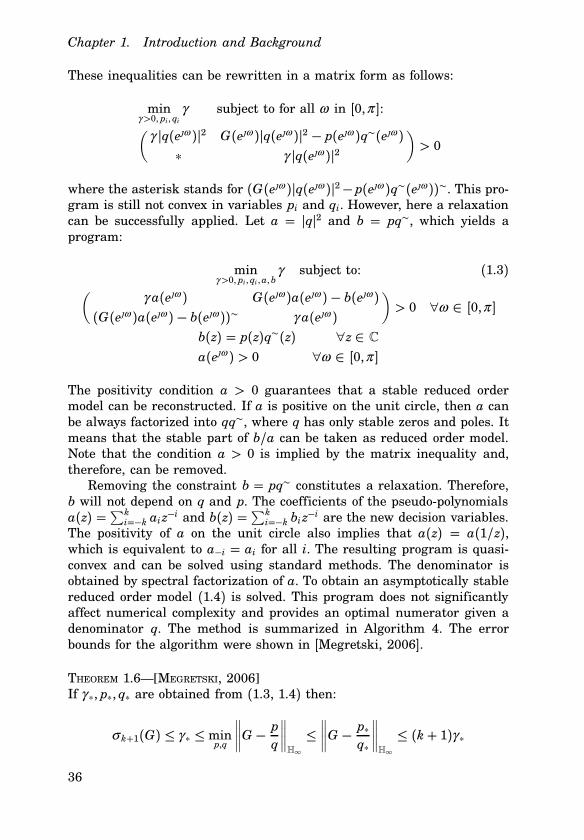
minγ>0, pi, qi
γ subject to for all ω in [0,π ]:(
γ pq(eω )p2 G(eω )pq(eω )p2 − p(eω )q∼(eω )
∗ γ pq(eω )p2
)> 0
where the asterisk stands for (G(eω )pq(eω )p2− p(eω )q∼(eω ))∼. This pro-gram is still not convex in variables pi and qi. However, here a relaxationcan be successfully applied. Let a = pqp2 and b = pq∼, which yields aprogram:
minγ>0, pi, qi,a,b
γ subject to: (1.3)(
γ a(eω ) G(eω )a(eω ) − b(eω )
(G(eω )a(eω ) − b(eω ))∼ γ a(eω )
)> 0 ∀ω ∈ [0,π ]
b(z) = p(z)q∼(z) ∀z ∈ C
a(eω ) > 0 ∀ω ∈ [0,π ]
The positivity condition a > 0 guarantees that a stable reduced ordermodel can be reconstructed. If a is positive on the unit circle, then a canbe always factorized into qq∼, where q has only stable zeros and poles. Itmeans that the stable part of b/a can be taken as reduced order model.Note that the condition a > 0 is implied by the matrix inequality and,therefore, can be removed.Removing the constraint b = pq∼ constitutes a relaxation. Therefore,
b will not depend on q and p. The coefficients of the pseudo-polynomialsa(z) =
∑ki=−k aiz
−i and b(z) =∑ki=−k biz
−i are the new decision variables.The positivity of a on the unit circle also implies that a(z) = a(1/z),which is equivalent to a−i = ai for all i. The resulting program is quasi-convex and can be solved using standard methods. The denominator isobtained by spectral factorization of a. To obtain an asymptotically stablereduced order model (1.4) is solved. This program does not significantlyaffect numerical complexity and provides an optimal numerator given adenominator q. The method is summarized in Algorithm 4. The errorbounds for the algorithm were shown in [Megretski, 2006].
THEOREM 1.6—[MEGRETSKI, 2006]If γ ∗, p∗, q∗ are obtained from (1.3, 1.4) then:
σ k+1(G) ≤ γ ∗ ≤ minp,q
∥∥∥∥G −p
q
∥∥∥∥H∞
≤
∥∥∥∥G −p∗
q∗
∥∥∥∥H∞
≤ (k+ 1)γ ∗
36

1.5 Quasi-Convex Optimization Approach to Model Reduction
Algorithm 4 Quasi-Convex Optimization (QCO) Approach to Model Re-duction
• Introduce new variables a =k∑i=−k
aiz−i b =
k∑i=−k
biz−i
• Solve the quasi-convex program
minγ>0,ai, bi
γ subject to for all ω in [0,π ]:(
γ a(eω ) G(eω )a(eω ) − b(eω )
(G(eω )a(eω ) − b(eω ))∼ γ a(eω )
)> 0
• Given a solution a∗, solve the spectral factorization problem a∗ =q∗q
∼∗
• Then given q∗, the numerator p∗ is computed as:
minp
∥∥∥∥G −p
q∗
∥∥∥∥∞
(1.4)
• The reduced order model is computed as G = p∗/q∗
Here minp,q
∥∥∥G − pq
∥∥∥H∞
is the optimal error of reduction, and σ k+1(G) is
the k+ 1-th largest Hankel singular value of G.
To obtain a numerically efficient program, the norm constraints are en-forced only on a finite frequency grid. To ensure stability the constrainta > 0 should be enforced for all the frequencies ω in [0,π ]. This can be doneefficiently using the Kalman-Yakubovitch-Popov lemma (see, Lemma 1.3).The approach was also extended to the parameterized model reduction
([Sou et al., 2005]) and frequency-weighted model reduction([Sandbergand Murray, 2007]).The approach presented in Chapter 2 is a relaxation of the QCO algo-
rithm. Therefore, a more detailed discussion on properties and interpre-tations of the method is presented not here, but in the upcoming chapters.
37

2
Semidefinite Hankel-type
Model Order Reduction
This chapter deals with a problem of scalable model reduction in the H∞norm. Two algorithms are proposed to address the problem. The algo-rithms perform matching of frequency response samples of a transfer func-tion. They result from a reformulation of the single-input-single-outputmodel reduction problem, which will be called a Hankel-type formulation.This formulation is obtained by introducing an auxiliary variable into theobjective function. In this formulation, two variables parameterize thedenominator of the reduced order model to some extent. One of thesevariables has only unstable modes. This is similar to Hankel model re-duction, in which a stable and an anti-stable functions are the decisionvariables (see, page 26 for the definition). Having this auxiliary variableallows two possibilities to obtain a convex problem: a relaxation and aniterative approach.The employed relaxation is related to both quasi-convex optimization
approach (QCO, in [Sou et al., 2008]) and Hankel model reduction ([Glover,1984]). The QCO is discussed in detail in this thesis (Algorithm 4 onpage 37) and Hankel model reduction is sketched in Section 1.2. In thesealgorithms, optimization is performed over stable and anti-stable transferfunctions. The stable one can be taken as a reduced order model. It canbe also shown that Hankel model reduction and the presented approachare relaxations themselves of the QCO algorithm.The proposed iterative algorithm solves a semidefinite program on ev-
ery iteration. It also converges given any feasible starting point. How-ever, given two different starting points, the converged solutions can bedifferent. A starting point can be computed from an asymptotically sta-ble low-order approximation of the full order model. Hence, the methodis able to potentially improve the quality of any model order reductionmethod. Given such initial point the stability constraint is expressed as
38

a positive real constraint, i.e., a non-convex constraint is replaced by asemidefinite one. Similar idea to express stability is employed in [Rantzerand Megretski, 1994] and [Henrion et al., 2003].It can not be claimed that the proposed relaxation always provides a
better model match than QCO Algorithm 4. Nevertheless, the proposedframework has a number of advantages:
• The quality of approximations obtained with QCO or the presentedrelaxation is comparable to the one of Hankel model reduction, whichis known to deliver very accurate solutions. However, the computa-tional cost of approximation may be significantly lower in comparisonto the one of Hankel model reduction.
• The proposed approach is a relaxation of the QCO algorithm, whichresults in a few advantages in comparison to the QCO algorithm.Firstly, a better numerical robustness, which is illustrated in de-tail in Example 2.1. Secondly, results of the parameterized modelreduction extension show a considerable improvement in the qual-ity of approximation. The parameterized model order reduction isinvestigated in Chapter 3.
• The presented iterative approach is a powerful tool when systemswith a structure are considered, i.e., decentralized structure, plant-controller systems, etc. The method is extended to such problems inChapters 4 and 5.
• For particular models, it is possible that the actual approximationerror of the proposed method is larger than the one of the QCOalgorithm. Nonetheless, the presented iterative approach is able tosignificantly reduce the loss of approximation quality, if it occursdue to the looser relaxation.
A direct generalization of the Hankel-type formulation to the multi-input-multi-output (MIMO) model reduction appears to be impossible.Therefore, the MIMO extensions of the proposed approaches are, in fact,slightly different algorithms. These are obtained using optimization tech-niques employed in [Sootla and Sou, 2010] and [Tobenkin et al., 2010].The chapter is organized as follows: the Hankel-type formulation of
model order reduction problem is presented in Section 2.1. Section 2.2describes the proposed relaxation for the single-input-single-output case.Different subsections are devoted to a system theoretic interpretation,a discussion on relationship to the QCO algorithm, implementation de-tails and different properties of the method. The iterative approach isbriefly discussed in Section 2.3. Section 2.4 describes a MIMO, frequency-weighted, positive real extensions to model order reduction. Numericalexamples are found in Section 2.5.
39
Chapter 2. Semidefinite Hankel-type Model Reduction
2.1 Hankel-type Formulation of Model Reduction Problem
The main focus of this chapter is reduction of discrete time models. Nev-ertheless, the algorithms can be extended to the continuous time case,as discussed in Section 2.5. Throughout the chapter, the assumptions arestandard, i.e., the full order model G is an asymptotically stable, causal,rational transfer function. In this section, it is also assumed that G is ascalar-valued transfer function. The reduction problem for such models isformulated as:
minp, q
qG − p/qqH∞
where p and q are FIR filters (i.e., p(z) =∑ki=0 piz
−i, q(z) =∑ki=0 qiz
−i)q has a stable inverse and p/q is a sought-for approximation. It is alsoassumed that the order of the full order model G is much larger than k.Minimizing the H∞ norm is usually rewritten as a minimization of an
approximation level γ subject to the norm constraints enforced only on
the unit circle D =z
∣∣∣pzp = 1and the stability constraint. Therefore, z
often will be substituted by eω . The resulting program reads as:
γmor = minp,q
γ subject to (2.1)
pG(eω )q(eω ) − p(eω )p < γ pq(eω )p ∀ω ∈ [0,π ]
q(z) has a stable inverse
The goal of this section is to show that the following formulation is equiv-alent to (2.1):
γ htf = minγ>0, p, q,ϕ
γ subject to (2.2)
pG(eω )q(eω )ϕ∼(eω ) − p(eω )ϕ∼(eω )p < γ Re (q(eω )ϕ∼(eω )) ∀ω ∈ [0,π ]
ϕ(z) has a stable inverse
where ϕ∼(z) is equal to ϕT (1/z). The program (2.2) is called a Hankel-type formulation of model order reduction. The name of the formulation isexplained in detail in Section 2.2. The main benefit of this formulation isthe absence of the absolute value function on the right hand side, whichgives two possibilities to obtain convex programs: a relaxation and aniterative approach, where ϕ is iterated over.The Hankel-type formulation is derived in a few simple steps. First,
consider a new variable ϕ , which is also an FIR filter of order k and
40

2.1 Hankel-type Formulation of Model Reduction Problem
it is non-zero on the unit circle. Introduce ϕ in (2.1) by replacing theconstraints
pG(eω )q(eω ) − p(eω )p < γ pq(eω )p ∀ω ∈ [0,π ]
with the equivalent ones:
pG(eω )q(eω )ϕ∼(eω ) − p(eω )ϕ∼(eω )p < γ pq(eω )ϕ∼(eω )p ∀ω ∈ [0,π ]
The resulting minimum will not change since ϕ can be always canceledout. Now replace pqϕ∼p with Re (qϕ∼).
minγ>0, p, q,ϕ
γ subject to (2.3)
pG(eω )q(eω )ϕ∼(eω ) − p(eω )ϕ∼(eω )p < γ Re (q(eω )ϕ∼(eω )) ∀ω ∈ [0,π ]
q(z) has a stable inverse and ϕ ,= 0 on [0,π ]
Note that the left-hand side of the inequality is non-negative and, there-fore, Re (qϕ∼) ≥ 0. Since ϕ and q are not equal to zero, as an artifacta positivity constraint Re (qϕ∼) > 0 for all the frequencies ω in [0,π ] isobtained. For further use, a simple lemma is required.
LEMMA 2.1Suppose q and ϕ are FIR filters of the same order. Assume also thatRe (qϕ∼) is positive for all the frequencies ω in [0,π ]. Then q has a stableinverse if and only if ϕ has a stable inverse.
Proof. It is straightforward to show that the inequality Re (qϕ∼) > 0implies that Re (qϕ−1) > 0 and Re (ϕq−1) > 0. If q−1 is stable, then thetransfer function ϕq−1 is positive real and, therefore, it has a stable in-verse. Hence, ϕ has a stable inverse. Similarly, the converse is shown.
LEMMA 2.2The optimal values γmor and γ htf are equal.
Proof. Due to Lemma 2.1 the program (2.3) is equivalent to (2.2). SinceRe (qϕ∼) ≤ pqϕ∼p for all q, ϕ and the frequencies ω in [0,π ], we have:
γ htf ≥ minγ>0, p, q,ϕ
γ subject to
pG(eω )q(eω )ϕ∼(eω ) − p(eω )ϕ∼(eω )p < γ pq(eω )ϕ∼(eω )p ∀ω ∈ [0,π ]
q(z) has a stable inverse and ϕ ,= 0 on [0,π ]
Now, we can divide both sides of the norm constraint with ϕ , and theminimization program reduces to (2.1). Therefore we have γmor ≤ γ htf.
41

Chapter 2. Semidefinite Hankel-type Model Reduction
To prove the converse, assume p∗q−1∗ is an optimal solution to the model
reduction problem (2.1) with the optimal approximation level γ ∗ = γmor.If we choose ϕ∗ = q∗, it is easy to verify that p∗, q∗, γ ∗, ϕ∗ satisfy theconstraints of (2.2). Thus γmor ≥ γ htf.Lemma 2.2 also provides an optimal choice of the auxiliary variable ϕ ,
which is simply equal to q. On the other hand, the variable pqp is replacedwith
Re(q ⋅
ϕ∼
pϕ p
)
This fact implies that the complex vector q is rotated in a way such thatRe (qϕ∼) becomes positive. The value ϕ∼/pϕ p defines the angle of such arotation. In the optimality, this angle is equal to − arg(q), which leavesonly a positive part in expression qϕ∼.
2.2 Semidefinite Hankel-type Model Reduction
First, a more systematic approach to convexification of the Hankel-type for-mulation (2.2) is employed, that is a relaxation. Introduce new variablesa :, qϕ∼ and b :, pϕ∼. Since p, q, and ϕ are FIR filter of order k, the newvariables are parameterized as a =
∑ki=−k aie
−iω and b =∑ki=−k bie
−iω .It is a standard technique in semidefinite programming and it yields aquasi-convex program:
γ cshmr = minγ>0, a,b
γ subject to (2.4)
pG(eω )a(eω ) − b(eω )p < γ Re (a(eω )) ∀ω ∈ [0,π ]
The non-convex conditions q and ϕ have only stable zeros, which corre-sponds to a (or qϕ∼) has exactly k stable zeros, is very hard to parame-terize in a convex manner in a and b. However, this constraint is actuallyimplied by positivity of the function Re (a).
LEMMA 2.3
Consider a function a =k∑
i=−k
aiz−i, the unit disc D and the unit circle D.
If Re (a(D)) > 0 then the pseudo-polynomial a has at most k zeros in D
and no zeros on D.
Proof. The function a(z) does not have zeros or poles on the unit circle(since Re (a(D)) > 0). It is also analytic in D except for a set of isolatedpoints. Thus by Cauchy’s argument principle Nz − Np = No where Nz isthe number of zeros in D, Np is the number of poles in D and No is a
42

2.2 Semidefinite Hankel-type Model Reduction
winding number of a(D) (number of times a(D) encircles the origin).Since Re (a(D)) > 0 for all the frequencies ω in [0,π ], the curve a(D)lies only in the right half plane and thus No = 0 and Nz = Np. Since Npis at most k, so is Nz.
REMARK 2.1If a is obtained using semidefinite programming, then the number of zerosin D is equal to k almost surely. The pseudo-polynomials with ak = 0(which would correspond to the case with Np ≤ k − 1 and Nz ≤ k − 1)constitute a measure zero subspace of the pseudo-polynomials with ak ,= 0.Therefore solutions of a semidefinite optimization procedure will haveak ,= 0 almost surely.
After solving (2.4), the denominator q is obtained by solving the equation:
a = qϕ∼ (2.5)
where ϕ , q have only stable zeroes and are the solutions to the non-symmetric spectral factorization problem (see, Section 1.3). Thus, the de-nominator q∗ is computed. The numerator is obtained from:
p∗ = argminp
qG − p/q∗qH∞ (2.6)
and the reduced order model is simply p∗/q∗. Finally, the semidefiniteHankel-type model reduction reads as solving (2.4,2.5,2.6) consecutively.
Tractable Algorithm and its Computational Complexity
The programs (2.4) and (2.6) have an infinite number of constraints, onefor each frequency ω in [0,π ]. Therefore, these are not tractable problems.However, given that G is a rational transfer function, the frequency re-sponse can not change too fast. It means that it may be sufficient to imposesome of the constraints of a finite number of frequencies ω iNi=1 ∈ [0,π ].The norm constraints (2.8) clearly can be relaxed this way. This is out-lined in SHMR Algorithm 5. The frequency griding is also a relaxation. Ifω iNi=1 is an N element subset of some countable set ω i
∞i=1, then by con-
struction γ Nshmr ≤ γ ∞shmr for any positive integer N. Moreover, if ω i∞i=1 is
dense in [0,π ] then γ ∞shmr = γ cshmr (γcshmr is the solution to (2.4)). In essence,
with a large enough N the theoretical value γ cshmr can be approximatedby γ Nshmr.To avoid over-fit, the number of points in the grid N should be at
least O(k2), where k is the order of the reduced model. This gridingapproach may create unstable approximations, therefore the positivityconstraint (2.9) is enforced for all the frequencies ω in [0,π ] using the
43
Chapter 2. Semidefinite Hankel-type Model Reduction
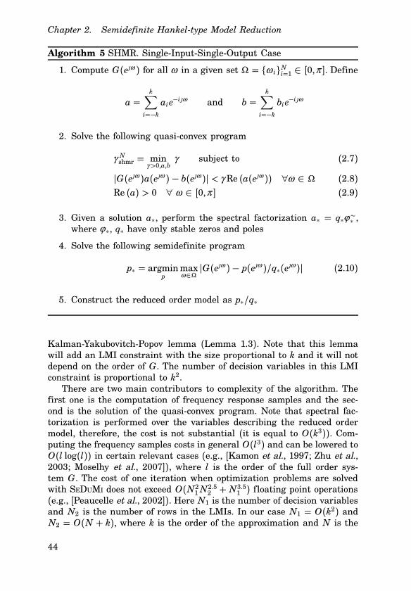
Algorithm 5 SHMR. Single-Input-Single-Output Case
1. Compute G(eω ) for all ω in a given set Ω = ω iNi=1 ∈ [0,π ]. Define
a =k∑
i=−k
aie−iω and b =
k∑
i=−k
bie−iω
2. Solve the following quasi-convex program
γ Nshmr = minγ>0,a,b
γ subject to (2.7)
pG(eω )a(eω ) − b(eω )p < γ Re (a(eω )) ∀ω ∈ Ω (2.8)
Re (a) > 0 ∀ ω ∈ [0,π ] (2.9)
3. Given a solution a∗, perform the spectral factorization a∗ = q∗ϕ∼∗ ,
where ϕ∗, q∗ have only stable zeros and poles
4. Solve the following semidefinite program
p∗ = argminp
maxω∈Ω
pG(eω ) − p(eω )/q∗(eω )p (2.10)
5. Construct the reduced order model as p∗/q∗
Kalman-Yakubovitch-Popov lemma (Lemma 1.3). Note that this lemmawill add an LMI constraint with the size proportional to k and it will notdepend on the order of G. The number of decision variables in this LMIconstraint is proportional to k2.There are two main contributors to complexity of the algorithm. The
first one is the computation of frequency response samples and the sec-ond is the solution of the quasi-convex program. Note that spectral fac-torization is performed over the variables describing the reduced ordermodel, therefore, the cost is not substantial (it is equal to O(k3)). Com-puting the frequency samples costs in general O(l3) and can be lowered toO(l log(l)) in certain relevant cases (e.g., [Kamon et al., 1997; Zhu et al.,2003; Moselhy et al., 2007]), where l is the order of the full order sys-tem G. The cost of one iteration when optimization problems are solvedwith SEDUMI does not exceed O(N21N
2.52 + N3.51 ) floating point operations
(e.g., [Peaucelle et al., 2002]). Here N1 is the number of decision variablesand N2 is the number of rows in the LMIs. In our case N1 = O(k2) andN2 = O(N + k), where k is the order of the approximation and N is the
44
2.2 Semidefinite Hankel-type Model Reduction
number of computed frequency samples. The overall cost is computed as
O(Nl log(l)) + O(k4N2.5 + N3.5)
Based on numerical simulations, the computationally heaviest part forlarge-scale systems (l > 10000) is the computation of frequency responsesamples of G.
Error Bounds and System Theory Interpretation of the Relaxation
SHMR Algorithm 5 is interesting due to its connection to Hankel modelreduction, which will be discussed in detail here. Rewriting the constraintsin (2.4) with a norm constraint yields:
minRe (a)>0, b
∥∥∥∥(G −
b
a
)a
Re (a)
∥∥∥∥∞
where a and b are pseudo-polynomials in z with degrees spanning from−k to k. Note that the weight a/Re (a) has the infinity norm bigger orequal to 1 since pap ≥ pRe (a)p for all the frequencies ω and thus:
minRe (a)>0, b
∥∥∥∥(G −
b
a
)a
Re (a)
∥∥∥∥∞
≥ minRe (a)>0, b
∥∥∥∥G −b
a
∥∥∥∥∞
Any pseudo-polynomial a with a positive real part can be decomposed intoq and ϕ as a = qϕ∼ using the spectral factorization. The FIR filters q andϕ have stable inverse, therefore q and ϕ∼ are coprime. It implies thatthe pseudo-polynomial b can be also decomposed using the Diophantineequation for some p and r:
b(z) = p(z)ϕ∼(z) + zk−1q(z)r(z)
where p, q, ϕ are FIR filters of order k, and r is an FIR filter of orderk − 1. Such a factorization has a unique solution in variables p and r.Hence, a following decomposition is available
b
a=p
q+zk−1r
ϕ∼
Going back to the optimization problems, the following inequality can beobtained by removing the positive real constraint.
minRe (a)>0, b
∥∥∥∥G −b
a
∥∥∥∥∞
≥ minq−1 , ϕ−1∈H∞
∥∥∥∥G −p
q−zk−1r
ϕ∼
∥∥∥∥∞
45

Chapter 2. Semidefinite Hankel-type Model Reduction
Since the optimization problem on the right hand side of the inequality isthe definition of Hankel model order reduction we have:
minRe (a)>0, b
∥∥∥∥(G −
b
a
)a
Re (a)
∥∥∥∥∞
≥ minp
q∈H∞
∥∥∥∥G −p
q
∥∥∥∥H
Thus, SHMR is Hankel model reduction with an extra weight in the ob-jective function (a/Re (a)) and an extra constraint on the denominator(Re (a) is positive for all the frequencies ω in [0,π ]). However, the distinc-tive part of the Hankel norm optimization, i.e., optimization over an extraanti-stable transfer function, is preserved in SHMR. Now we are ready toformulate the main theorem of the section.
THEOREM 2.1Assume (2.4), (2.5), (2.6) were consecutively solved providing as a solutionγ cshmr, a∗, b∗, p∗, q∗. Let γmor also be the optimal approximation level from(2.1). Then the following error bounds hold:
σ k+1(G) ≤ γ cshmr ≤ γmor ≤ qG − p∗/q∗q∞ (2.11)
qG − p∗/q∗q∞ ≤ (k+ 1)γcshmr (2.12)
where σ k+1(G) is k+ 1-st Hankel singular value of G.
Proof. The idea of the proof is taken from [Megretski, 2006].First, consider the lower bounds (2.11). The inequality γmor ≤ qG −
p∗/q∗q∞ follows from the fact that γmor is a solution of (2.1) and thereforeγmor is a minimum value for all possible p and q.The inequality γ cshmr ≤ γmor is satisfied by construction. Recall that (2.1)
is general and (2.2) is Hankel-type formulations of model reduction. TheHankel-type formulation (2.2) has the optimal approximation level γ htf.Furthermore, γmor = γ htf by Lemma 2.2. Since the proposed method (2.4)is a relaxation of the Hankel-type formulation (2.2), then γ cshmr ≤ γ htf andthe inequality follows.Finally, the inequality σ k+1(G) ≤ γ cshmr follows from the fact that
σ k+1(G) is a lower bound on Hankel model reduction and as discussedabove is a lower bound on SHMR.Now, prove the upper bound (2.12). Note that
qG − b∗/a∗q∞ ≤ γ cshmr
a∗ and b∗ can be uniquely decomposed as mentioned above:
b∗
a∗
=p
q∗
+zk−1r
ϕ∼
46

2.2 Semidefinite Hankel-type Model Reduction
where p and r are FIR filters of order k and k − 1 respectively. The in-equality ∥∥G − p/q∗ − z
k−1r/ϕ∼∥∥∞≤ γ cshmr
implies that ∥∥zk−1r/ϕ∼∥∥H≤ γ cshmr
by the famous Adamian-Arov-Krein theorem (see, for example [Zhou et al.,1996]). A consequence to the theorem states that there exist such D that
∥∥zk−1r/ϕ∼ + D∥∥∞≤ kγ cshmr
Combining this bound with the triangle inequality yields:∥∥∥∥G −
p+ Dq∗
q∗
∥∥∥∥∞
≤ (k+ 1)γ cshmr
Since the numerator p∗ is obtained by means of optimization (2.6), theupper bound follows.
REMARK 2.2The obtained upper bounds are conservative, since no information aboutthe full order model G is used. However, an upper bound is required asa guarantee, that the employed relaxation will not create unreasonableapproximations. The quality of a relaxation is estimated on numericalexamples.
The difference between QCO Algorithm 4 and SHMR is a symmetry con-straint a(z) = a(1/z). It is straightforward to show that if a(z) = a(1/z),then the imaginary part of a(z) on the unit circle is equal to zero. There-fore the real part of a on the unit circle is equal a. Therefore, if thissymmetry constraint is added to the SHMR algorithm, the QCO algo-rithm will be obtained. Therefore, the following chain of inequalities isavailable:
γmor ≥ γ cqco = mina>0,b
∥∥∥∥G −b
a
∥∥∥∥∞
≥ γ cshmr = minRe (a)>0,b
∥∥∥∥(G −
b
a
)a
Re (a)
∥∥∥∥∞
≥
≥ σ k+1(G) = minp/q∈H∞
∥∥∥∥G −p
q
∥∥∥∥H
It is also possible to compare the upper bounds, given a specific way tocompute the reduced order model. For example, if the reduced order mod-els are obtained as in (2.6) then:
(k+ 1)γ cqco ≥ (k+ 1)γcshmr ≥ γmor ≥ γ cqco ≥ γ cshmr
47
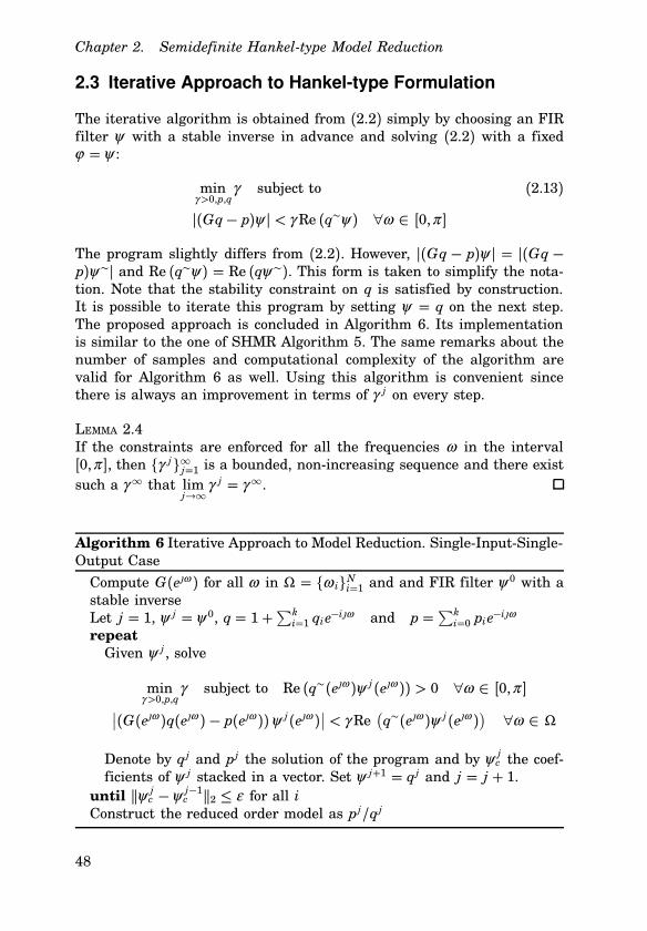
Chapter 2. Semidefinite Hankel-type Model Reduction
2.3 Iterative Approach to Hankel-type Formulation
The iterative algorithm is obtained from (2.2) simply by choosing an FIRfilter ψ with a stable inverse in advance and solving (2.2) with a fixedϕ =ψ :
minγ>0,p,q
γ subject to (2.13)
p(Gq− p)ψ p < γ Re (q∼ψ ) ∀ω ∈ [0,π ]
The program slightly differs from (2.2). However, p(Gq− p)ψ p = p(Gq −p)ψ ∼p and Re (q∼ψ ) = Re (qψ ∼). This form is taken to simplify the nota-tion. Note that the stability constraint on q is satisfied by construction.It is possible to iterate this program by setting ψ = q on the next step.The proposed approach is concluded in Algorithm 6. Its implementationis similar to the one of SHMR Algorithm 5. The same remarks about thenumber of samples and computational complexity of the algorithm arevalid for Algorithm 6 as well. Using this algorithm is convenient sincethere is always an improvement in terms of γ j on every step.
LEMMA 2.4If the constraints are enforced for all the frequencies ω in the interval[0,π ], then γ j∞j=1 is a bounded, non-increasing sequence and there existsuch a γ ∞ that lim
j→∞γ j = γ ∞.
Algorithm 6 Iterative Approach to Model Reduction. Single-Input-Single-Output Case
Compute G(eω ) for all ω in Ω = ω iNi=1 and and FIR filter ψ 0 with astable inverseLet j = 1, ψ j =ψ 0, q= 1+
∑ki=1 qie
−iω and p =∑ki=0 pie
−iω
repeat
Given ψ j , solve
minγ>0,p,q
γ subject to Re (q∼(eω )ψ j(eω )) > 0 ∀ω ∈ [0,π ]∣∣(G(eω )q(eω ) − p(eω ))ψ j(eω )
∣∣ < γ Re(q∼(eω )ψ j(eω )
)∀ω ∈ Ω
Denote by qj and pj the solution of the program and by ψ jc the coef-
ficients of ψ j stacked in a vector. Set ψ j+1 = qj and j = j + 1.until qψ j
c −ψ j−1c q2 ≤ ε for all i
Construct the reduced order model as pj/qj
48

2.4 Model Reduction Extensions
Proof. First, prove that γ j∞j=1 is a bounded and non-increasing sequenceof real numbers. It is actually sufficient to prove for an arbitrary j thatγ j ≥ γ j+1. Let ψ j+1 = qj , choose qj+1 = qj and pj+1 = pj , then
p(Gqj − pj)qj p ≤ γ j+1Re ((qj)∼qj) = γ j+1pqj p2 ∀ω ∈ [0,π ]
are the constraints of the program at ( j + 1)-th step. By construction ofthe j-th step:
pGqj − pj p ≤ γ j pqj p
we can always choose γ j+1 such that γ j ≥ γ j+1. Since any γ j is a positivenumber, the sequence γ j∞j=1 is bounded.Finally since γ j∞j=1 is bounded and non-increasing, then there exist
a limit point γ ∞.The choice of the stopping criterion is guided by the following argu-
ment. If ψ j = ψ j−1 for some j, then it means that γ j = γ j+1 due to thedefinition of ψ j . It also implies, that γ j = γ ∞. On the other hand, if con-vergence is checked only with respect to γ j , that is, checking if γ j = γ j+1,then it can not be guaranteed that γ j = γ ∞.The properties of the limit function p∞/q∞ is an intriguing topic, how-
ever, such analysis is difficult since the behaviour of the limit is highlydependent on the initial point. If minimized over ψ as well, the pro-gram (2.13) is non-convex, non-smooth optimization and can have nu-merous local minima. Any iterative approach to solve the problem doesnot, generally, converge to globally optimal solution. Therefore, in orderto evaluate if a solution is globally optimal, it is required to evaluate theproperties of the H∞ optimal solution. These are unknown, to the au-thor’s best knowledge. It can be only claimed that p∞/q∞ is an order kstable transfer function. Due to these reasons, the approach is coupledwith SHMR Algorithm 5, where a starting point is located close in H∞ toa decent suboptimal solution.
2.4 Model Reduction Extensions
Many details are simply sketched in this section due to resemblance to theother cases. The derivation of the iterative algorithms for positive-real andfrequency-weighted extension is not presented for the same reason.
Multi-Variable Extensions
As mentioned above, the multi-input-multi-output (MIMO) extension isdifferent in some aspects from its SISO counterpart. However, the mainattribute is preserved: optimization over anti-stable transfer functions.
49

Chapter 2. Semidefinite Hankel-type Model Reduction
Assume G ∈ Hv$m∞ , where v is the number of outputs and m is the numberof inputs, and the problem is formulated as:
minP,Q
∥∥G − PQ−1∥∥H∞
where P =∑ki=0 Piz
−i ∈ Hv$m∞ , Q =∑ki=0 Qiz
−i ∈ Hm$m∞ , and Q−1 isa stable transfer function. In this case, the degree of the reduced ordertransfer function PQ−1 can not be set freely. It may be shown that theorder of PQ−1 is generally equal to the degree of det(Q), which is equal tokm ([Kailath, 1980]). Therefore, the order can be set only to a multiple ofm. Moreover, the parameterization PQ−1 does not describe all the stablemodels of order km, and it can happen that the “best” reduced ordermodels can not be parameterized in this manner.We start similarly to the SISO case and introduce into the program a
new frequency dependent function Φ =∑ki=0 Φiz
−i ∈ Hm$m∞ , which has astable inverse, as:
minγ>0, P,Q,Φ
γ subject to
Φ(GQ − P)∼(GQ − P)Φ∼ < γ 2ΦQ∼QΦ∼ ∀ω ∈ [0,π ]
Q−1, Φ−1 are stable
This program is equivalent to the original one, since it is possible to cancelout Φ from both sides of inequalities and eliminate Φ from the program.In the SISO case the next step was replacing pqϕ∼p with Re (qϕ∼). Thisreplacement had an interpretation of a rotation of the vector q such thatthe phase of qwould be cancelled byϕ . The concept of phase is not uniquelydefined for the MIMO case and such replacement appears to be impossible.Therefore, first, the relaxation is performed and after that a tractableprogram is obtained. Introduce new variables A :, QΦ∼ and B :, PΦ∼
and obtain:
γmr = minγ>0, A, B
γ subject to
(GA− B)∼(GA− B) < γ 2A∼A ∀ω ∈ [0,π ]
A has km stable and km unstable zeros
To address the quadratic constraint the following relation is used (e.g.,[Sootla and Sou, 2010], [Tobenkin et al., 2010]), which is valid for arbitrarymatrices X and Y:
X ∼Y + Y∼X − Y∼Y ≤ X ∼X (2.14)
50

2.4 Model Reduction Extensions
It is obtained from (X − Y)∼(X − Y) ≥ 0. Using this inequality meansthat yet another variable R is introduced, which is an initial guess on A:
γmb = minγ>0, A, B,R
γ subject to
(GA− B)∼(GA− B) < γ 2 (R∼A+ A∼R − R∼R) ∀ω ∈ [0,π ]
A have km stable and km unstable zeros
The relaxed programs are equivalent, i.e., γmb = γmr. It is also comforting,that if G, A, B are all scalar valued and R = (A + A∼)/2 then γmb isequal to γ cshmr from (2.4). Unlike the SISO case, the MIMO programs arenon-convex, and finding the global minimum is not guaranteed. In orderto obtain a tractable program, let R = rI, where r is a positive, scalar-valued function. In this case, the program is quasi-convex and the LMIformulation can be obtained using the Schur complement as follows.
γmimo = minγ>0, A, B, r
γ subject to (2.15)(
γ 2rI GA− B
(GA− B)∼ A+ A∼ − rI
)> 0 ∀ω ∈ [0,π ]
where the constraint r > 0 is now implied in the LMI. The program (2.15)is the MIMO version of (2.4). To guarantee the condition on zeros of A,a general version of Lemma 2.3 can be formulated, where Cauchy’s argu-ment principle is applied to the determinant of A.
LEMMA 2.5
Consider an m by m transfer function A =k∑i=−k
aizi, a unit disc D and a
unit circle D. If Re (det(A(D))) > 0 then the pseudo-polynomial A hasat most km zeros in D and no zeros on D.
A setting with matrix-valued R can be tackled in the same manner. In thiscase, the condition R∼A+ A∼R > 0 implies that A has km stable zeros, ifR has km stable zeros. An iterative procedure can be also applied to therelaxed problem by setting R = A on the next iteration step. However, itseems more reasonable to iterate not in the space of the relaxed variables,but in the space of the actual variables using the iterative approach. TheMIMO approach is summarized in Algorithm 7.Regarding the error bound the results for the MIMO case are not as
impressive as for the SISO case. Since a restriction is applied to obtaina quasi-convex program, it can not be stated that the obtained approxi-mation level γmimo is equal to γmb and it is a lower bound on the modelreduction problem.
51
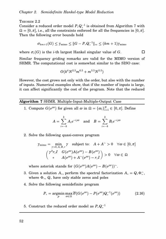
Chapter 2. Semidefinite Hankel-type Model Reduction
THEOREM 2.2Consider a reduced order model P∗Q
−1∗ is obtained from Algorithm 7 with
Ω = [0,π ], i.e., all the constraints enforced for all the frequencies in [0,π ].Then the following error bounds hold
σ km+1(G) ≤ γmimo ≤ qG − P∗Q−1∗ q∞ ≤ (km + 1)γmimo
where σ i(G) is the i-th largest Hankel singular value of G.
Similar frequency griding remarks are valid for the MIMO version ofSHMR. The computational cost is somewhat similar to the SISO case:
O(k4N2.5m6.5 +m3.5N3.5)
However, the cost grows not only with the order, but also with the numberof inputs. Numerical examples show, that if the number of inputs is large,it can affect significantly the cost of the program. Note that the reduced
Algorithm 7 SHMR. Multiple-Input-Multiple-Output Case
1. Compute G(eω ) for given all ω in Ω = ω iNi=1 ∈ [0,π ]. Define
A =k∑
i=−k
Aie−iω and B =
k∑
i=−k
Bie−iω
2. Solve the following quasi-convex program
γmimo = minγ>0, A,B, r
γ subject to: A+ A∼ > 0 ∀ω ∈ [0,π ](
γ 2ri I G(eω )A(eω ) − B(eω )
∗ A(eω ) + A∼(eω ) − ri I
)> 0 ∀ω ∈ Ω
where asterisk stands for (G(eω )A(eω ) − B(eω ))∼.
3. Given a solution A∗, perform the spectral factorization A∗ = Q∗Φ∼∗ ,
where Φ∗, Q∗ have only stable zeros and poles
4. Solve the following semidefinite program
P∗ = argminP
maxω∈Ω
σ (G(eω ) − P(eω )Q−1∗ (eω )) (2.16)
5. Construct the reduced order model as P∗Q−1∗
52

2.4 Model Reduction Extensions
model can be parameterized as G = Q−1P and a similar algorithm may bederived as well. In this case, m is the number of outputs in the complexityestimate.To derive the iterative algorithm for multi-variable models similar to
Algorithm 6, it is required to approach the problem from a different sideas well. The general formulation of model reduction problem reads as:
minγ>0,P,Q
γ subject to: Q−1 is stable
(GQ − P)∼(GQ − P) < γ 2Q∼Q ∀ω ∈ [0,π ]
And it is required only to tackle the quadratic constraint, which is doneagain using (2.14), i.e., using the inequality
R∼Q + Q∼R − R∼R ≤ Q∼Q
The MIMO version of the iterative Algorithm 6 is obtained by pre-com-puting R and fixing it in the optimization program as in Algorithm 8.The condition Q∼R + (Q∼R)∼ > 0 is equivalent to QR−1 + (QR−1)∼ > 0.Therefore, if R−1 is fixed and it is stable, then QR−1 is strictly positivereal and Q−1 is stable. Similar convergence analysis may be applied toMIMO models as in SISO iterative Algorithm 6.
REMARK 2.3The presented algorithms may be applied to the SISO models as well.
Algorithm 8 Iterative Approach to Model Reduction. Multiple-Input-Multiple-Output Case
Compute G(eω ) for all ω in Ω = ω iNi=1 and R0 with a stable inverse
Let j = 1, R j = R0, Q =∑ki=0 Qie
−iω and P =∑ki=0 Pie
−iω
repeat
Given R j , solve
minγ>0,P,Q
γ subject to: Q∼R j + (Q∼R j)∼ > 0 ∀ω ∈ [0,π ]
(GQ − P)∼(GQ − P) < γ 2((R j)∼Q + Q∼R j − (R j)∼R j
)∀ω ∈ Ω
Denote by Q j and P j the solution of the program and by R jc thecoefficients of R j stacked in matrix. Set R j+1 = Q j and j = j + 1
until qR jc − Rj−1c qF ≤ ε for all i
Construct the reduced order model as P j(Q j)−1
53
Chapter 2. Semidefinite Hankel-type Model Reduction
Indeed, in the case when Algorithm 8 applied to a SISO model:
minγ>0,q,p
γ subject to:
pGq− pp2 < γ 2 (2Re (ψ ∼q) −ψ ∼ψ ) ∀ω ∈ [0,π ]
In order to make the notation consistent, R is replaced withψ . To comparethe right-hand side to the SISO program (2.13), it is required to multiplywith pψ p2 from both sides. Now, it becomes straightforward to verify that
pψ p2(2Re (ψ ∼q) −ψ ∼ψ ) ≤ (Re (ψ ∼q))2
for any ψ . The last inequality is equivalent to
(Re (ψ ∼q))2 − 2Re (ψ ∼q)pψ p2 + pψ p4 = (Re (ψ ∼q) − pψ p2)2 ≥ 0
The MIMO techniques are more restrictive than the SISO ones. However,a generalization of the SISO method directly to the MIMO case appearsto be impossible.
Frequency-Weighted Model Order Reduction
The frequency-weighted model reduction is formulated as:
minp,q
∥∥∥∥w(G −
p
q
)∥∥∥∥H∞
where p =∑ki=0 piz
−i, q =∑ki=0 qiz
−i and q and w are stable with stableinverses. The conditions on the weight w are not restrictive. If a transferfunction y−1 has an unstable pole, then the required w can be obtainedby the spectral factorization yy∼, which does not affect the H∞ norm. Thederivation of the algorithm in the SISO case is very similar to the originalone and results in a program:
minγ>0,a,b
γ subject to (2.17)
pw(eω ) (G(eω )a(eω ) − b(eω ))p ≤ γ Re (a(eω )) ∀ω ∈ [0,π ]
In the multiple-input-multiple-output case, one sided weights are handledthe same way. Therefore, consider the two sided case:
minp,q
∥∥Wo(G − PQ−1
)Wi
∥∥H∞
54
2.4 Model Reduction Extensions
The weights Wi and Wo are asymptotically stable with asymptotically sta-ble inverses W−1
i and W−1o . First, rewrite the constraints in a more useful
form using a series of equivalent transformations:
(Wo(GQ − P)Q−1Wi)
∼Wo(GQ − P)Q−1Wi ≤ γ 2 I
(Wo(GQ − P))∼Wo(GQ − P) ≤ γ 2Q∼W−∼
i W−1i Q
multiply from the right with Φ∼ and from the left with Φ both sides ofthe inequality:
(Wo(GQ − P)Φ∼)∼Wo(GQ − P)Φ
∼ ≤ γ 2ΦQ∼W−∼i W
−1i QΦ∼
Now employing the relaxation yields:
(Wo(GA− B))∼Wo(GA− B) ≤ γ 2A∼W−∼
i W−1i A
Apply a similar series of inequalities as in the unweighted MIMO case,namely:
(X − Y)∼Z(X − Y) ≥ 0\ X ∼ZX ≥ Y∼ZX + X ∼ZY − Y∼ZY
In our case Z is equal to WiW∼i , and X is equal to A. Let Y be a positive
scalar-valued frequency dependent variable r, and obtain a program:
minγ>0,A,B,r
γ subject to for all ω in [0,π ]:
(Wo(GA− B)Wi)∼Wo(GA− B)Wi ≤ γ 2(r(W−1
i AWi +W∼i A
∼W−∼i ) − r2 I)
The quasi-convex program is obtained using the Schur’s complement. Theiterative approach can be obtained using the same techniques. Theoreti-cal results similar to ones proposed in [Sandberg and Murray, 2007] and[Sootla and Rantzer, 2009], where the frequency-weighted versions of theQCO algorithms were reported, can be shown in the same manner.
Positive Real Constraint
In order to enforce positive-realness, a well-known relationship will beused, i.e., a transfer function G is strictly positive real if and only if (G −I)(I+G)−1 has the H∞ norm less than one. Substituting p/q for G yields:
Re(p(eω )
q(eω )
)> 0 ∀ω ∈ [0,π ] Z[
∥∥∥∥p− q
p+ q
∥∥∥∥H∞
< 1
55

Chapter 2. Semidefinite Hankel-type Model Reduction
In the presented framework, the second condition is easier to modelby introducing an FIR filter ϕ with a stable inverse as follows:
∣∣∣∣(p− q)ϕ∼
(p+ q)ϕ∼
∣∣∣∣ < 1 ∀ω ∈ [0,π ]
For any such ϕ , such that Re ((p + q)ϕ∼) is positive for all the fre-quencies in [0,π ], the constraint presented below will ensure the positiverealness of p/q :
p(p− q)ϕ∼p < Re ((p+ q)ϕ∼) ∀ω ∈ [0,π ]
Using the relaxation as in the previous sections yields a positive-real im-posing condition:
pa− bp < Re (a+ b) ∀ω ∈ [0,π ] (2.18)
In the multiple-input-multiple-output case similar ideas are used. An-other scalar frequency-dependent variable r is introduced as:
(rI A− B
∗ A+ B + (A+ B)∼ − rI
)> 0 ∀ω ∈ [0,π ]
2.5 Examples
These examples are set to estimate the actual relaxation gap in the Hankel-type approximation and a possible improvement by the iterative approachto any reduction procedure. The Hankel model reduction is implementedby a MATLABTM routine HANKELMR. The SISO version of SHMR Algorithm 5and QCO Algorithm 4 are implemented using a cutting plane algorithm(for more details, see [Sou, 2008]), the MIMO and positive-real versions ofSHMR are implemented using the interior point solver SEDUMI [Sturm,1999] and the parser YALMIP [Löfberg, 2004].
Data Pre-Processing and Frequency Griding
If a continuous-time model is approximated, it should be first discretizedin order to apply the proposed approaches (as well as the QCO method).The discretization is performed, while warping around a particular fre-quency ω 0 in the process, using the formula:
s = µz− 1z+ 1
, where µ =ω 0
tan(ω 0Ts/2)
56
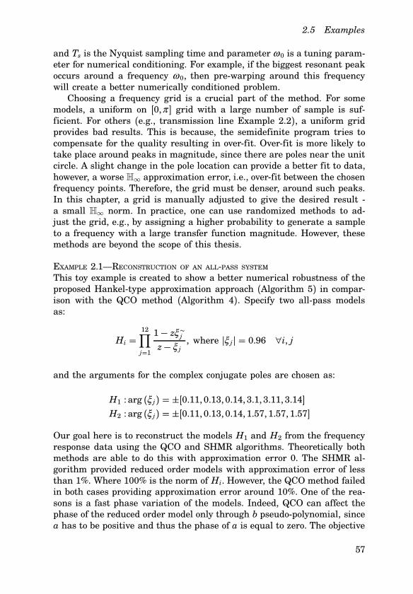
2.5 Examples
and Ts is the Nyquist sampling time and parameter ω 0 is a tuning param-eter for numerical conditioning. For example, if the biggest resonant peakoccurs around a frequency ω 0, then pre-warping around this frequencywill create a better numerically conditioned problem.Choosing a frequency grid is a crucial part of the method. For some
models, a uniform on [0,π ] grid with a large number of sample is suf-ficient. For others (e.g., transmission line Example 2.2), a uniform gridprovides bad results. This is because, the semidefinite program tries tocompensate for the quality resulting in over-fit. Over-fit is more likely totake place around peaks in magnitude, since there are poles near the unitcircle. A slight change in the pole location can provide a better fit to data,however, a worse H∞ approximation error, i.e., over-fit between the chosenfrequency points. Therefore, the grid must be denser, around such peaks.In this chapter, a grid is manually adjusted to give the desired result -a small H∞ norm. In practice, one can use randomized methods to ad-just the grid, e.g., by assigning a higher probability to generate a sampleto a frequency with a large transfer function magnitude. However, thesemethods are beyond the scope of this thesis.
EXAMPLE 2.1—RECONSTRUCTION OF AN ALL-PASS SYSTEMThis toy example is created to show a better numerical robustness of theproposed Hankel-type approximation approach (Algorithm 5) in compar-ison with the QCO method (Algorithm 4). Specify two all-pass modelsas:
Hi =
12∏
j=1
1− zξ∼jz− ξ j
, where pξ j p = 0.96 ∀i, j
and the arguments for the complex conjugate poles are chosen as:
H1 : arg (ξ j) = ±[0.11, 0.13, 0.14, 3.1, 3.11, 3.14]
H2 : arg (ξ j) = ±[0.11, 0.13, 0.14, 1.57, 1.57, 1.57]
Our goal here is to reconstruct the models H1 and H2 from the frequencyresponse data using the QCO and SHMR algorithms. Theoretically bothmethods are able to do this with approximation error 0. The SHMR al-gorithm provided reduced order models with approximation error of lessthan 1%. Where 100% is the norm of Hi. However, the QCO method failedin both cases providing approximation error around 10%. One of the rea-sons is a fast phase variation of the models. Indeed, QCO can affect thephase of the reduced order model only through b pseudo-polynomial, sincea has to be positive and thus the phase of a is equal to zero. The objective
57

Chapter 2. Semidefinite Hankel-type Model Reduction
of a variable is to match the magnitude of b, since Hi are all-pass, i.e.,qHiq∞ " 1. It results in ratio between maximal and minimal coefficientsof a larger than 104. The SHMR approach does not restrict a to be positiveand phase can be affected both from b and a variables.Another way to see how SHMR can avoid numerical problems is the
ability to choose ϕ freely in relationship a = qϕ∼, the QCO approach isobliged to preserve the symmetry of a. Therefore in case of large ratio ofcoefficients of q, the SHMR method does not necessarily square this ratioin comparison to the QCO.
EXAMPLE 2.2—TRANSMISSION LINE MODELINGThis example is described in [Chahlaoui and Dooren, 2002] and the refer-ences therein. A transmission line is a 2-input-2-output model, which isdescribed by the following system of differential equations:
Ex = Ax + Bu
y = Cx
where matrix E is invertible, but badly conditioned. The order of theoriginal model is 256. The comparison is performed in percent relative tothe H∞ norm of the full order model G.Scalar-valued Model Reduction. In this example, only the 2, 2-entry
of the transfer function is being reduced. The H∞ norms of the approxima-tion errors are given in Table 2.1. Here, HMR stands for Hankel model re-duction. The quality of Hankel approximations is generally worse than thequality of optimization approaches. However, applying Algorithms 2 and 6reduces this conservatism. Recall, that in Algorithm 2 the denominatoris fixed and is obtained from the Hankel approximation, in Algorithm 6,
Table 2.1 Approximation errors in percent in Example 2.2
Reduction order k 8 13 16 18
σ k+1(G) 10.83% 3.16% 0.43% 0.31%
lower bound of QCO Alg. 4 10.87% 3.32% 0.90% 0.41%
HMR 21.70% 6.35% 0.95% 0.65%
HMR+Algorithm 2 15.70% 4.02% 0.71% 0.47%
HMR+Algorithm 6 13.70% 3.95% 0.69% 0.43%
QCO Algorithm 4 11.61% 3.92% 1.16% 0.43%
SHMR Algorithm 5 11.27% 3.47% 0.55% 0.42%
58
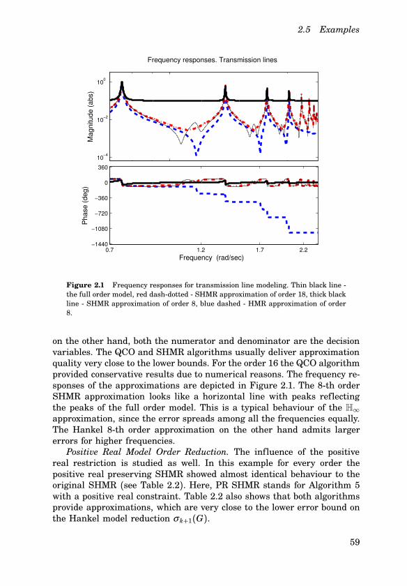
2.5 Examples
10−4
10−2
100
Ma
gn
itu
de
(a
bs)
0.7 1.2 1.7 2.2−1440
−1080
−720
−360
0
360
Ph
ase
(d
eg
)
Frequency responses. Transmission lines
Frequency (rad/sec)
Figure 2.1 Frequency responses for transmission line modeling. Thin black line -the full order model, red dash-dotted - SHMR approximation of order 18, thick blackline - SHMR approximation of order 8, blue dashed - HMR approximation of order8.
on the other hand, both the numerator and denominator are the decisionvariables. The QCO and SHMR algorithms usually deliver approximationquality very close to the lower bounds. For the order 16 the QCO algorithmprovided conservative results due to numerical reasons. The frequency re-sponses of the approximations are depicted in Figure 2.1. The 8-th orderSHMR approximation looks like a horizontal line with peaks reflectingthe peaks of the full order model. This is a typical behaviour of the H∞
approximation, since the error spreads among all the frequencies equally.The Hankel 8-th order approximation on the other hand admits largererrors for higher frequencies.Positive Real Model Order Reduction. The influence of the positive
real restriction is studied as well. In this example for every order thepositive real preserving SHMR showed almost identical behaviour to theoriginal SHMR (see Table 2.2). Here, PR SHMR stands for Algorithm 5with a positive real constraint. Table 2.2 also shows that both algorithmsprovide approximations, which are very close to the lower error bound onthe Hankel model reduction σ k+1(G).
59

Chapter 2. Semidefinite Hankel-type Model Reduction
Table 2.2 Approximation errors in percent in Example 2.2. Positive Real ModelReduction
Reduction order k 1 2 3 4 5
σ k+1(G) 51.19% 33.50% 33.50% 21.16% 21.16%
SHMR Alg. 5 51.20% 33.51% 33.51% 21.18% 21.18%
PR SHMR 51.20% 33.51% 33.52% 21.18% 22.02%
Table 2.3 Approximation errors in percent in Example 2.2. Multi-Variable ModelReduction
Reduction order km 2 4 6 8 10
σ km+1(G) 33.50% 21.17% 16.78% 10.84% 7.29%
MIMO SHMR Alg. 7 51.19% 33.50% 33.50% 21.16% 21.16%
MIMO SHMR+Alg. 8 51.17% 33.50% 21.17% 16.91% 14.55%
HMR 65.45% 41.35% 32.80% 21.18% 14.65%
Multi-Variable Model Reduction. Here, the entire two-input-two-outputmodel of transmission lines is considered. The numerical computationsshow that the iterative approach considerably improves the quality of theinitial SHMR methods quality (see Table 2.3). Here, HMR stands for Han-kel model reduction. In this example, at most 15 iterations of Algorithm 8were used. MIMO SHMR Algorithm 7 presents conservatism for orders 6to 10. Algorithm 8 is able to reduce this conservatism for higher orders.The quality of the iterative Algorithm 8 applied to the SHMR method ismore consistent with Hankel model reduction quality. However, none ofthe methods are able to reach the lower bound σ km+1(G).
2.6 Conclusion and Discussion
In this chapter, an approach to model reduction of linear time invariantsystems has been presented. The method requires only the frequency re-sponse samples to obtain an approximation and guarantees stability inthe H∞ sense. The minimization is performed in a Hankel-type norm andthe accuracy of the algorithm is expected to be close to the optimal Hankelone. The computational complexity of the algorithm is lower than the oneof optimal Hankel approximation method for certain applications. There-fore, by sacrificing some quality, efficiency is gained.
60

2.6 Conclusion and Discussion
Although the presented method is different from its predecessor, QCO,and provides a better guarantee on approximation quality (the upperbound on the error), there is no guarantee that the actual approxima-tion quality is better. In fact, in many examples considered in preparationof this manuscript the approximation errors match or there is only anepsilon improvement. Nevertheless, aforementioned advantages outweighpossible drawbacks.Although the lack of symmetry in the denominator seems to be a minor
advantage, it provides a better numerical robustness. Moreover, in para-meterized extension, this relaxation delivers significant improvement. Adetailed discussion about the parameterized model reduction is availablein Chapter 3.The convergence properties of the iterative approach have to be eval-
uated as well. The method does not generally converge to the global min-imum, since the model reduction is a non-convex problem. Therefore, anestimate of approximation quality improvement would be a decent result,especially given SHMR as an initial point. These qualities are also im-portant since the iterative approach can be easily extended to the modelswith a structure as shown in Chapter 5.
61

3
Parameterized Model Order
Reduction
Parameterized model reduction is arguably a more important tool in mod-eling and design than H∞ model reduction. Parameterized model reduc-tion deals with linear time-invariant models, which depend on certaindesign parameters. Since parameters of the models are subject to changeor fine-tuning over time, it is often required to obtain a family of mod-els which describe a particular system in various settings. The models inthis family should preferably have the same orders, therefore, parameter-ized model reduction is used to model such families in a more convenientway. Extensive research using the Krylov techniques was performed forvarious applications, such as micro-electro-mechanical systems or MEMS([Rudnyi et al., 2006]), radio-frequency (RF) inductors ([Daniel and White,2003]), interconnects ([Daniel et al., 2002; Daniel et al., 2004; Li et al.,2005b; Li et al., 2005a]), general linear systems ([Farle et al., 2008; Fenget al., 2009; Li et al., 2007]) and non-linear systems ([Bond and Daniel,2005]). Another interesting approach is being developed in [Lefteriu et al.,2010; Lefteriu and Mohring, 2010]. In this approach, reduced models areobtained by interpolating the frequency response, which is calculated (oridentified from a real system) for a finite number of frequencies.The main focus of this chapter is extension to parameterized LTI sys-
tems of the algorithms from Chapter 2. Therein, the original model reduc-tion problem was reformulated by adding an extra frequency-dependentvariable ϕ . Performing a semidefinite relaxation to the problem yieldedthe semidefinite Hankel-type model reduction (SHMR Algorithm 5 onpage 44). Whereas, applying an iterative approach to the new formula-tion formed Algorithm 6 on page 48. Note that when an extra constraintto SHMR Algorithm 5 is added, then a method from [Sou et al., 2008] isobtained. The approach from [Sou et al., 2008] is sketched in the thesisas QCO Algorithm 4 on page 37.
62

3.1 Preliminaries and Problem Formulation
The extension to parameterized model order reduction itself is not theonly result of this chapter. A theoretical statement regarding the approx-imation quality of reduced order models with respect to parameters isalso derived. The error bounds are also valid for the parameterized QCOmethod, although such bounds were not shown in the original work [Souet al., 2008].Numerical simulations show that the restriction, which separates the
SHMR and QCO algorithms, results in a worse approximation quality ofthe parameterized QCO method. Performance improvement of such mag-nitude was not expected since non-parameterized LTI model reduction didnot exhibit similar results.Each of the methods in the framework has its benefits and drawbacks.
For example, both parameterized QCO and parameterized SHMR deliverbounds on approximation quality, but can not provide explicit parameter-dependent models. Whereas, the parameterized extension of iterative Al-gorithm 6 can provide such models. However, the quality of approximationmay be worse than SHMR and QCO have.The chapter is organized as follows: the problem is formulated and the
non-parameterized method from Chapter 2 is revised in Section 3.1. Theparameterized extension is described in Section 3.2, where the main the-oretical result shown as well. In Section 3.3 the problem of reconstructingexplicit parameter dependent models is discussed. The most promising ap-proach in this direction is the iterative approach to parameterized modelreduction, which is also presented. The relationship between QCO, SHMRand the iterative approach is outlined therein, which explains why a cer-tain method can provide a better match for certain models. The frameworkis illustrated on numerical examples in Section 3.4.
3.1 Preliminaries and Problem Formulation
Given a family of linear time-invariant (LTI) models G(z,θ), which areassociated with a parameter θ , the following assumptions are made:
• The parameter θ is constant over time
• The parameter θ is a real scalar and belongs to the interval [0,π ]
• The coefficients of the transfer function G depend smoothly on θ
• For every fixed θ the model G(z,θ) is an asymptotically stable ra-tional transfer function with a frequency variable z
• The transfer function G is scalar-valued
63

Chapter 3. Parameterized Model Order Reduction
The framework is still valid for a vector-valued θ . The restriction to theinterval [0,π ] can always be achieved by a linear variable change if θbelongs to any other bounded interval. The extension to matrix-valuedfunctions in the parameterized case is achieved in the same way as inChapter 2 once the framework for the scalar-valued functions is obtained.The conservatism of the matrix-valued extension in Chapter 2 manifestsitself in the same way for the parameterized case.Given a family of models G(z,θ), our main goal is to find another
family G(z,θ) that is close to G for all possible θ . Such a family can befound using a min-max criterion:
minG is stable
maxθ∈[0,π ]
qG(z,θ) − G(z,θ)q∞
The L∞ norm is a maximization itself with respect to the frequency ωin the interval [0,π ]. Therefore, this formulation is similar to the non-parameterized case.
γ pmor = minpi j ,qi j
maxω ,θ∈[0,π ]
pG(eω ,θ) − p(ω ,θ)/q(ω ,θ)p (3.1)
where p/q is stable
For parameterized models, stability is defined as stability for every pa-rameter θ . The functions p and q are expressed as follows:
p(ω ,θ) =k0∑
i=0
k1∑
j=0
pi jFi(ω )H j(θ)
q(ω ,θ) =k0∑
i=0
k1∑
j=0
qi jFi(ω )H j(θ)
The basis functions Fn describe the dependence on the frequency variableω . Therefore it is reasonable to choose Fn = e−nω . Still, if required, it ispossible to choose a different basis. If extra information about a system isknown, then a few possibilities are described in [Heuberger et al., 2005].The basis functions Hn describe the dependence on the parameter θ . Inthe thesis Hn = cos(nθ) was chosen to use. However, in this case as well,different choices are possible. For example, one can set Hn = θ n.To avoid any confusion in terminology in the various fields of engineer-
ing, the term “multi-variate pseudo-polynomial” will refer to a pseudo-polynomial of two or more variables (i.e. ω 1, ω 2 and so forth). The term“multi-variable” will be used for matrix-valued transfer functions G(⋅).
64

3.2 Parameterized SHMR
Hankel-type Model Reduction
The methods from Chapter 2 are the foundation of the entire framework.Therefore, to simplify the presentation of the parameterized extension,they are revised. A non-parameterized formulation of (3.1) is as follows:
γmor = minγ>0,p,q
γ subject to (3.2)
pG(eω )q(eω ) − p(eω )p < γ pq(eω )p ∀ω ∈ [0,π ]
p(eω ) =
k∑
i=0
pie−iω q(eω ) =
k∑
i=0
qie−iω
where q(z) has a stable inverse. In Chapter 2 it was shown that the latterprogram is equivalent to:
γ htf = minp,q,ϕ
γ subject to (3.3)
pG(eω )q(eω )ϕ∼(eω ) − p(eω )ϕ∼(eω )p < γ Re (q(eω )ϕ∼(eω )) ∀ω ∈ [0,π ]
where ϕ−1(z) is a stable transfer function, ϕ∼(z) = ϕ(1/z) and
ϕ =k∑
i=0
ϕ ie−iω p =
k∑
i=0
pie−iω q =
k∑
i=0
qie−iω
The equivalence is understood as γmor = γ htf. Moreover, for every solu-tion (pmor, qmor, γmor) of the problem (3.2), there exists ϕ such that thequadruple (pmor, qmor, γmor, ϕ) satisfies the conditions of (3.3). And if thequadruple (γ htf, phtf, qhtf, ϕhtf) is an optimal solution to (3.3), then thetriple (γ htf, phtf, qhtf) is an optimal solution to (3.2). And finally, it may beshown that if ϕ has a stable inverse then so does q due to the positivityof Re (qϕ∼) for all the frequencies in [0,π ].The iterative approach is obtained by setting the variable ϕ equal to
1 in the optimization. On the next iteration ϕ is set equal to the solutionon the current iteration q until the solution q becomes equal to ϕ . Therelaxation (the SHMR algorithm) is obtained by introducing new vari-ables a :, qϕ∼ and b :, pϕ∼. The SHMR approach is summarized inAlgorithm 9.
3.2 Parameterized Semidefinite Hankel-type ModelReduction
Introduce the notation ω = ω ,θ ∈ [0,π ]2, where θ is a parameter, ω is
65

Chapter 3. Parameterized Model Order Reduction
Algorithm 9 Semidefinite Hankel-type Model Reduction
1. Compute the frequency response G(eω ) for every ω in Ω = ω iNi=1
2. Solve the relaxed problem:
mina,b
γ subject to Re (a) > 0 ∀ω ∈ [0,π ] (3.4)
pG(eω )a(eω ) − b(eω )p < γ Re (a(eω )) ∀ω ∈ Ω
3. Compute the denominator q from the spectral factorization a = qϕ∼
4. For a given q, solve
minpmaxω∈Ω
pG(eω ) − p(eω )/q(eω )p
5. Set the reduced order model G = p/q
a frequency domain variable. Introduce the pseudo-polynomials
a(ω ) =
k0∑
i=−k0
k1∑
j=0
ai j e−iω cos( jθ) b(ω ) =
k0∑
i=−k0
k1∑
j=0
bi j e−iω cos( jθ)
and substitute them into (3.4) which results in:
mina,b
γ subject to Re (a) ≥ µ ∀ω ∈ [0,π ]2 (3.5)
pG(ω )a(ω ) − b(ω )p < γ Re (a(ω )) ∀ω ∈ Ω (3.6)
where µ is a positive pre-defined scalar and needed as a technical re-quirement, Ω = ω i
Ni=1 is a pre-defined finite grid and with a slight
abuse of notation G(ω ) stands for G(eω ,θ). The non-negative constraintRe (a)−µ ≥ 0 is convex, but not tractable for a multi-variate a. Therefore,a semidefinite Sum-Of-Squares (SOS) constraint will be used instead, i.e.,Re (a) − µ is an SOS. It is a standard way to approach the problem andis called an “SOS relaxation” (see, Theorem 1.5 for the actual algebraicconstraints). As before, the positivity constraint Re (a) > 0 has the in-terpretation of a stability ensuring constraint. It can be shown that ifRe (a) > 0, then for every fixed θ the pseudo-polynomial a has k stablezeros and k unstable ones. Given a, a stable model can be reconstructed.In the non-parameterized case, the next step after solving (3.5-3.6)
would be the non-symmetric spectral factorization of a. However, if there
66

3.2 Parameterized SHMR
Algorithm 10 Parameterized SHMR
1. Compute the frequency response G(ω ) for every ω = ω ,θ in Ω =ω i
Ni=1
2. Solveγ Npshmr = min
a,bγ subject to
Re (a) ≥ µ ∀ω ∈ [0,π ]2
pG(ω )a(ω ) − b(ω )p < γ Re (a(ω )) ∀ω ∈ Ω
3. For a particular θ , compute the denominator qθ from aθ = qθϕ∼θ(e.g., [Fairman et al., 1992])
4. For a particular θ , compute the numerator pθ from
pθ = argminp
maxω∈Ω
pbθa−1θ − pq−1θ p
where p is parameterized as p = p0 + p1e−ω + ⋅ ⋅ ⋅+ pke−k0ω
are two or more variables, even the symmetric spectral factorization hasmuch stricter conditions. For a general case, such conditions are describedin [Dritschel and Woerdeman, 2005] and for the two dimensional case(one parameter in our notation), refer to [Geronimo and Lai, 2006]. Theconditions are not convex in the chosen variables (the coefficients of a) andare equivalent to a rank constraint. Given such a complexity, obtaininga reasonable relaxation seems to impossible. An approximate solution tothe multi-variate symmetric spectral factorization may be found in, forexample, [Ekstrom and Woods, 1976]. In this section, the multi-variatespectral factorization problem is avoided. For a fixed θ , let aθ = a(⋅,θ)and bθ = b(⋅,θ) and the method can be summarized in Algorithm 10.As the output of the algorithm, two mappings are obtained. In realiza-
tion mappings pθ , qθ can be stored as look-up tables for required values ofθ . Or one can store pseudo-polynomials a and b, and obtain the requiredpθ , qθ when needed. The latter approach is tractable, since a and b havelow order and the factorization can be done cheaply. The final optimiza-tion problem is a second order cone program and is also much cheaperthan the relaxed program.
Error Bounds
If in Algorithm 10 all the constraints are enforced for all the frequenciesω ∈ [0,π ]2, then γ Npshmr is denoted as γ cpshmr. The main theoretical result
67
Chapter 3. Parameterized Model Order Reduction
of this chapter is outlined in the next statement:
THEOREM 3.1Consider Algorithm 10 with the full sampling (the constraints are enforcedfor all the frequencies ω ∈ [0,π ]2) with the solution γ cpshmr, bθ , aθ and pθ ,qθ . The following inequalities hold:
1. maxθ∈[0,π ]
σ k0+1(G(⋅,θ)) ≤ γ cpshmr
2. γ cpshmr ≤ maxθ∈[0,π ]
qG − pθ/qθq∞
3. maxθ∈[0,π ]
qG − pθ/qθq∞ ≤ (k0 + 1)γ cpshmr
where σ k0+1(G(⋅,θ)) is the (k0 + 1)-th largest Hankel singular value ofG(⋅,θ), k0 is the order of pseudo-polynomials pθ , qθ with respect to z.
Proof.
1. For every θ , Algorithm 10 is essentially Hankel model reduction withextra restrictions, as it was shown for the non-parameterized case in Chap-ter 2. Therefore, for every θ , the inequality σ k0+1(G(⋅,θ)) ≤ γ cpshmr is sat-isfied. By taking the maximum over all θ , the result is achieved.
2. Consider two optimization programs:
minbmax
θ∈[0,π ]qG − b/aθq∞ min
pmax
θ∈[0,π ]qG − p/qθq∞
where qθ and aθ are defined as above. Since aθ = qθϕ∼θ the variable bcan be chosen such that, the stable part of b/aθ is equal to p/qθ and theanti-stable part equal to zero. Clearly, the left-most problem has morefreedom and its solution is equal to γ cpshmr. The right-most program hasthe solution equal to max
θ∈[0,π ]qG− pθ/qθq∞. Thus the inequality is obtained.
3. Let the anti-stable part of bθ/aθ be G−. Since qG(⋅,θ) − bθ/aθq∞ ≤γ cpshmr, by the celebrated AAK theorem, there exists a matrix K (θ) suchthat the following bound is satisfied.
qG−qH ≤ γ cpshmr [ qG− + Kq∞ ≤ k0γcpshmr
By the triangular inequality we have:
qG(⋅,θ) − pθ/qθq∞ ≤ qG(⋅,θ) − bθ/aθq∞+
+ qbθ/aθ − pθ/qθq∞ ≤ (k0 + 1)γ cpshmr
68

3.3 Computation of Explicit Parameter Dependent Models
and since it is always possible to pick pθ such that
qbθ/aθ − pθ/qθq∞ ≤ qG− + Kq∞ ≤ k0γcpshmr
After taking the maximum over θ the result follows.It is a direct generalization of the non-parameterized error bounds.
However, in the parameterized case, it is not clear if γ cpshmr is smallerthan γ pmor from (3.1). An SOS relaxation is employed, i.e., Re (a)−µ is anSOS and rather than Re (a) − µ is non-negative. Despite the name, theSOS relaxation is actually a restriction on decision variables compared tothe non-negative condition. Hence, as opposed to Algorithm 9, it can notbe guaranteed that γ cpshmr is a lower error bound on the parameterizedmodel reduction program (3.1).
REMARK 3.1The extension to the multi-variable (MIMO) systems is done by employingthe techniques from Chapter 2 to obtain a tractable algorithm. The errorbounds are essentially the same
1. maxθ∈[0,π ]
σ k+1(G(⋅,θ)) ≤ γ cpshmr
2. γ cpshmr ≤ maxθ∈[0,π ]
qG − pθ q−1θ q∞
3. maxθ∈[0,π ]
qG − pθ q−1θ q∞ ≤ (k+ 1)γ
cpshmr
However, now pθ and qθ are matrix valued functions and k is the order ofpθ q
−1θ , not the order of pθ and qθ with respect to z. If the order of pθ and
qθ with respect to z is set to k0 and qi j ∈ Rm$m, then the order k of pθ q−1θ
is generally equal to k0m.
REMARK 3.2The Quasi-Convex Optimization (QCO) approach by [Sou et al., 2008] is aspecific case of the algorithm described in the this section. It requires anadditional constraint on a, namely a∼(z) = a(z), or aT(1/z) = a(z), thenIm (a) = 0, and Re (a) = a. All the theoretical results of SHMR approachare still valid for the QCO method.
3.3 Computation of Explicit Parameter Dependent Models
The output of SHMR Algorithm 10 is a model b/a, where a and b arepseudo-polynomials. For every value of the parameter θ , the model b/a
69
Chapter 3. Parameterized Model Order Reduction
Algorithm 11 Dominant part heuristic
1. For every parameter θ compute the dominant part of G(⋅,θ)
2. Build a transfer function Gd(z,θ) by interpolation of dominant partwith respect to θ
3. Solve the following approximation problem using one of the pre-sented algorithms:
minp,qqG − Gdp/qq∞
REMARK. At the final step, one can solve instead:
minp,qqGG−1d − p/qq∞
The choice of the program is left to the designer
contains stable and unstable poles. The actual approximations p/q are, infact, obtained for every given θ , which is not the desired output. The de-sired output would be a model p/q, where p and q are pseudo-polynomialsin both ω and θ . Such models significantly simplify the analysis and speedup the simulations as well. Moreover, in some applications it may be re-quired to compute such models. In this section, a few techniques arepresented, which can produce parameter dependent models with explicitdependence on the parameter.
Dominant Part Heuristics
Extraction of the dominant poles is a simple, but an important heuristicin the parameterized reduction. By itself, it does not provide an explicitparameter-dependent model, however, coupled with the iterative approachpresented in the sequel it delivers very competitive solutions. This ap-proach can considerably speed up the computation of SHMR solutions aswell. The dominant poles are usually defined as the poles near the unitcircle which contribute to the Bode magnitude plot in the form of peaks.The dominant part is a collection of such poles. The approach is outlinedin Algorithm 11.An argument can be made that after computation of the dominant
part most of the work (if not all of it) has been done. However, in theparameterized case the dependence of the rest of the model (without thedominant part) may be complicated as well due to the parameter vari-ations. Therefore, a simple interpolation may not give a good result interms of accuracy on the validation stage.
70

3.3 Computation of Explicit Parameter Dependent Models
Algorithm 12 Parameterized Iterative Approach to Model ReductionCompute the frequency response samples G(ω ) for every ω = ω ,θ inΩ = ω i
Ni=1
Given an initial point ϕ 0, set j = 1, ϕ j = ϕ 0
repeat
Solve
γ Nprd = minp,q
γ subject to
Re (q∼ϕ j) ≥ µ ∀ω ∈ [0,π ]2
p(G(ω )q(ω ) − p(ω ))ϕ j(ω )p < γ Re (q∼(ω )ϕ j(ω )) ∀ω ∈ Ω
Denote ϕ jc all the coefficients of ϕ j stacked in a vector. Set j = j + 1and ϕ j = q
until qϕ jc −ϕ j−1c q2 ≤ εConstruct the reduced order model as p/q
Iterative Approach to Parameterized Model Reduction
In the non-parameterized framework, the iterative approach is obtainedby fixing ϕ in (3.3). Similarly, Algorithm 12 is derived. If it is possible toestimate ϕ(ω ) in advance, then an explicit parameter-dependent modelp/q can be computed.In order to enforce the condition Re (qϕ∼) ≥ µ for all the frequencies
in [0,π ]2, an explicit parameter dependence of ϕ is also required. In theparameterized case, the SHMR algorithm can not be used for these pur-poses, since it does not provide this type of solution. The obvious choiceis iterating, while starting with ϕ equal to one. However, it can be verycostly if the number of iterations is large.The main conservatism of setting ϕ " 1 is inability of tracking the
dominant poles, which corresponds to fast phase variations (this case isdiscussed in [Sootla and Sou, 2010]). If Re (q) is positive, then the phaseis confined to the interval between [−π/2,π/2]. Note, by extracting thedominant part, the phase variations are reduced. Therefore, the dominantpart heuristic described above can be used to significantly reduce suchconservatism, and thus reduce the number of iterations.Besides delivering explicit parameter-dependent functions, there is an-
other advantage of the iterative approach in comparison to QCO. It is amore efficient parameterization, which may result in a lower computa-tional cost. Indeed, consider a transfer function G, the numerator and thedenominator of which depend as (trigonometric) polynomials of order r ona parameter. To approximate it with the QCO approach, it is required to
71

Chapter 3. Parameterized Model Order Reduction
create pseudo-polynomials a and b of order 2r in parameter dependence,since a = qq∼. The iterative approach, on the other hand, requires polyno-mials of order r to parameterize the reduced order model. If ϕ " 1, thenthe SOS constraints for the iterative method will be much smaller thanthe ones for QCO method. Then again, there is no extra advantage, interms of accuracy, of the iterative method in comparison to the SHMR. Itoccurs due to the fact that SHMR is a relaxation of the iterative approach.Therefore, the SHMR algorithm will always deliver the most accurate ap-proximation among all the methods in the framework.
Interpolation of an SHMR solution
After SHMR Algorithm 10 is solved, transfer functions pθ (z,θ i)/qθ (z,θ i)for some i are obtained. If a transfer function with an explicit depen-dence on θ is required, it can be obtained by interpolation of coefficientsof pθ (z,θ i)/qθ (z,θ i). However, in this case, stability for every value of θ ican not be guaranteed. Such an approach is less accurate than the dom-inant part heuristic. In the dominant part heuristic only the dominantpart is interpolated. The rest of the model is computed with stability andnorm constraints. It can be done with iterative Algorithm 12, which alsocounteracts possibly occurring interpolation errors. Although, the inter-polation of the SHMR solution is still a valid approach, it is not consideredin the current thesis due to stability problems.
3.4 Implementation and Examples
The methods were implemented using YALMIP ([Löfberg, 2004]) and SE-DUMI ([Sturm, 1999]). Recall that the described method addresses thereduction of discrete-time systems, therefore in order to reduce a contin-uous time model it is discretized using a bi-linear transformation (as inChapter 2). Regarding the positivity constraint a few options are describedin [Dumitrescu, 2007, Chapter 3].
Computational Complexity
There are two main contributors to the complexity of the methods. Thefirst one is computing the frequency samples which is O(l3) for each fre-quency point, with l being the order of the original model. In many cases,it can be lowered to O(l log(l)) even for dense models (for example, us-ing [Kamon et al., 1997; Moselhy et al., 2007; Zhu et al., 2003]). Thesecond one is the cost of the optimization algorithm. It does not exceedO(N21N
2.52 + N3.52 ) with N1 being the number of decision variables and
N2 the number of rows in the LMI constraints, when the method is im-plemented with SEDUMI (see [Peaucelle et al., 2002]). In parameterized
72

3.4 Implementation and Examples
reduction, N1 will be O((k0 + 1) ⋅ ⋅ ⋅ (kn + 1))2, if the parameter θ is in Rn
and N2 = O(N + (k0 + 1) ⋅ ⋅ ⋅ (kn + 1)). The reduced model orders ki ≪ land N is the number of points in the grid. Note that number of frequencysamples N generally does not depend on the order of the system. Typi-cally, the larger number N is required, when some poles are close to theunit circle. The total cost will be
O(l log(l)N) + O(((k0 + 1) ⋅ ⋅ ⋅ (kn + 1))4N2.52 + N3.52 )
Based on the numerical simulations, the semidefinite program now ismuch more costly than in the non-parameterized case. The main reasonfor such a cost is the positivity constraint, which can create intractableprograms for a large number of the parameters and large orders of thepseudo-polynomials. The quadratic term ((k0+1) ⋅ ⋅ ⋅ (kn+1))2 comes fromthe positivity constraint enforced for all the frequencies in [0,π ]2. If an-other strategy is used, for example enforcing the positivity constraint ona parameter grid, then N1 = O((k0 + 1) ⋅ ⋅ ⋅ (kn + 1) + (k0 + 1)2) andN2 = O(N + k0). Which significantly reduces the cost, however, for someparameter values an unstable model can be obtained.
Possible Applications
Consider a linear parameter-varying (LPV) model, which depends on aparameter θ . For these models it is typically assumed that θ is a timedependent function. A very simple example of a linear parameter-varyingmodel is a time-varying one, with time t as a parameter. Modeling ofsuch systems can be approached by assuming the parameter is constant.After that, the proposed model reduction framework can be used. Thisapproach is typically called a local approach to linear parameter-varyingsystem modeling (see, [Petersson and Löfberg, 2009; Tóth et al., 2009] andthe references therein for other approaches). The positivity condition inthe method is equivalent to stability of the function G(⋅,θ) ∈ H∞ for anyfixed θ , which is a necessary condition for the global LPV stability.It is also quite tempting to apply the presented approach to n-D sys-
tem modeling (see [Beck et al., 1995; Wu and Lam, 2008] for existingapproaches). In this case, the basis functions should be modified. Nowboth variables are varying on the unit circle
Fs = e−sω Hs = e
−sθ
The basis can be analytically extended to the complex plane (z1, z2), wherez1 corresponds to eω and z2 corresponds to eθ . At the same time, thepositivity constraint Re (a) > 0 guarantees that the zeros of a lie in
D = (z1, z2)∣∣pz1p ≤ 1, pz2p = 1 ∪ (z1, z2)
∣∣ z1 = 0, pz2p ≤ 1
73

Chapter 3. Parameterized Model Order Reduction
which is a stability domain for the 2-D transfer functions ([Jury, 1978]).Using the iterative approach, it is possible to obtain explicit dependenceon variables ω and θ , and thus z1 and z2. In the case, for 2-D transferfunctions the order of a state-space realization of the system may be higherthan r1 + r2, where r1 is the number of basis functions Fs and r2 is thenumber of basis function Hs. Furthermore, obtaining a general minimalrealization is still an open question in the theory. However, it is shownthat there are systems that do not have a real valued realization of orderr1 + r2. A counter example may be found in [Kung et al., 1977]. Where analgorithm to obtain a state-space realization of order min(2r1+r2, r1+2r2)is described.Both applications are merely possibilities of the further developments
of the framework. In both cases, there are some difficulties, which areunavoidable at the moment.
EXAMPLE 3.1—EFFICIENCY OF PARAMETERIZATIONTo illustrate the parameterization issues, consider this toy example. Con-sider a transfer function:
G(z,θ) =ω 21
s2 + 2ζ 1ω 1s+ω 21
ω 22s2 + 2ζ 2ω 2s+ω 22
where ω 1 = 1, ω 2 = 3, ζ 1 = 0.1+0.9θ , ζ 1 = 0.1+0.9(1−θ) and θ ∈ [0, 1].If a state-space modeling approach is used, for example [Petersson andLöfberg, 2009], then the required parameterization is a linear one withA(θ) = A0 + A1θ and B,C, D matrices constant. Using the describedframework, the required parameterization is of order 2 for iterative Algo-rithm 12 and SHMR Algorithm 10, while the QCO method requires pa-rameterization of order 4. However, [Petersson and Löfberg, 2009] is nota semidefinite approach, which means that the computational efficiencyis lower than in the presented framework. The approximation errors aregiven in Table 3.1. The notation (4, 1) means that the frequency compo-nent e−ω has the order 4 and parameter θ has a basis of order 1.
EXAMPLE 3.2—DEFORMABLE MIRROR MODELINGThe following model was studied in [Giselsson, 2006] and obtained bymeans of a finite element modeling approach that resulted in a system ofsecond-order differential equations:
I x +α Λ2 x + Λ = Fu
y = FT x
where a model has 420 sensors and actuators, 2000 states, and the frictioncoefficient α is chosen as a modeling parameter. The comparison of the
74

3.4 Implementation and Examples
0 0.5 1 1.5 2 2.5 3
1
2
3
4
Frequency (rad/sec)
Ma
gn
itu
de
(a
bs)
Figure 3.1 Frequency response of models in Example 3.1 for different values ofparameters. The curves are solid blue for θ < 0.5 and dotted green for θ > 0.5
approximation error is performed in percent, where 100% is the maximumH∞ norm of the models on the training grid.A single entry of the corresponding transfer matrix is considered. The
objective is to obtain a family of low-order models that depend on α whichbelongs to the interval [0.01, 0.06]. The models are trained (computed) onthe parameter α = 0.01, 0.02, 0.03, 0.04, 0.05, 0.06 (the training grid).The validation is performed on another grid α = 0.015, 0.025, 0.035, 0.045,0.055. For every value of the parameter, 300 frequency response samplesare computed. For iterative Algorithm 12, only one iteration is computedwith ϕ " 1.The results of reduction for different orders is found in Tables 3.2
and 3.3. The QCO reduced order models had almost the same approxi-mation quality for orders (10, 1), (13, 1) and (16, 1). At the same time,significantly improving if the order of the parameter is raised to 2. Thisbehaviour signals that the order equal 1 for the parameter is not suf-ficiently large in this example. On the other hand, using Algorithm 12
Table 3.1 Approximation errors in Example 3.1
Identification orders (4, 1) (4, 2) (4, 4)
[Petersson and Löfberg, 2009] (error in H2) ( 0 ( 0 ( 0
QCO (error in H∞) 0.441 0.025 ( 0
Iter. Alg. 12 (error in H∞) 0.0557 ( 0 ( 0
SHMR Alg. 10 (error in H∞) 0.0337 ( 0 ( 0
75

Chapter 3. Parameterized Model Order Reduction
1.4 1.6 1.8 2 2.2 2.4 2.60
0.05
0.1
0.15
0.2
0.25
0.3
0.35
0.4
Reduced Order Models on the Validation Grid
Frequency (rad/sec)
Ma
gn
itu
de
(a
bs)
Figure 3.2 Frequency responses for α = 0.025, 0.045 (values belong to the val-idation grid) of the SHMR reduced order (thick green lines), the reduced ordermodel obtained with iterative Algorithm 12 (blue solid lines), the QCO reducedorder (dashed thin blue lines) and the full order (black crosses) models. Order ofreduction is set to (16,1).
(with ϕ " 1) it is possible to achieve a decent quality if the order is setto (16, 1), but the approximations are very conservative with lower ordersof frequency variable z. The SHMR method is consistently better thaniterative Algorithm 12 and the QCO, both on the training and the vali-dation grids. Except for the order (10, 2) where the approximation errorof SHMR is larger than the one of QCO on the validation grid. In fact,even (10, 1) SHMR approximation is better than (10, 2) SHMR approxi-mation. It means that over-fit has occurred and there is not sufficientlymany constraints for this order. Over-fit can be cured in this case by set-
Table 3.2 Approximation errors on the training grid (in %) in Example 3.2.
Orders (10, 1) (10, 2) (13, 1) (13, 2) (16, 1) (16, 2)
SHMR Alg. 10 0.99 1.24 1.11 0.93 0.99 1.03
QCO 11.19 3.81 8.46 1.23 9.75 1.11
Iter. Alg. 12 14.74 14.70 12.41 12.39 1.42 1.07
76
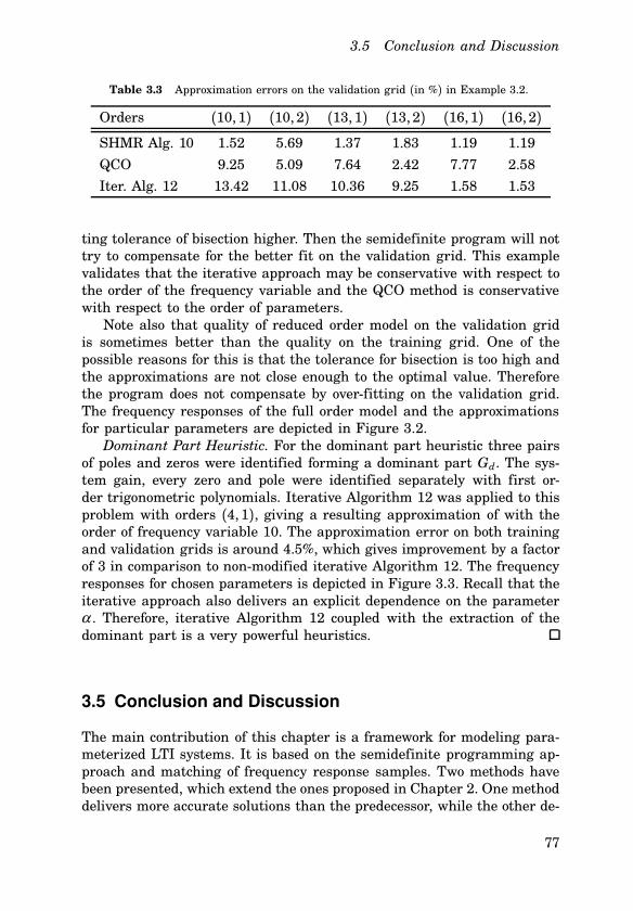
3.5 Conclusion and Discussion
Table 3.3 Approximation errors on the validation grid (in %) in Example 3.2.
Orders (10, 1) (10, 2) (13, 1) (13, 2) (16, 1) (16, 2)
SHMR Alg. 10 1.52 5.69 1.37 1.83 1.19 1.19
QCO 9.25 5.09 7.64 2.42 7.77 2.58
Iter. Alg. 12 13.42 11.08 10.36 9.25 1.58 1.53
ting tolerance of bisection higher. Then the semidefinite program will nottry to compensate for the better fit on the validation grid. This examplevalidates that the iterative approach may be conservative with respect tothe order of the frequency variable and the QCO method is conservativewith respect to the order of parameters.Note also that quality of reduced order model on the validation grid
is sometimes better than the quality on the training grid. One of thepossible reasons for this is that the tolerance for bisection is too high andthe approximations are not close enough to the optimal value. Thereforethe program does not compensate by over-fitting on the validation grid.The frequency responses of the full order model and the approximationsfor particular parameters are depicted in Figure 3.2.Dominant Part Heuristic. For the dominant part heuristic three pairs
of poles and zeros were identified forming a dominant part Gd. The sys-tem gain, every zero and pole were identified separately with first or-der trigonometric polynomials. Iterative Algorithm 12 was applied to thisproblem with orders (4, 1), giving a resulting approximation of with theorder of frequency variable 10. The approximation error on both trainingand validation grids is around 4.5%, which gives improvement by a factorof 3 in comparison to non-modified iterative Algorithm 12. The frequencyresponses for chosen parameters is depicted in Figure 3.3. Recall that theiterative approach also delivers an explicit dependence on the parameterα . Therefore, iterative Algorithm 12 coupled with the extraction of thedominant part is a very powerful heuristics.
3.5 Conclusion and Discussion
The main contribution of this chapter is a framework for modeling para-meterized LTI systems. It is based on the semidefinite programming ap-proach and matching of frequency response samples. Two methods havebeen presented, which extend the ones proposed in Chapter 2. One methoddelivers more accurate solutions than the predecessor, while the other de-
77

Chapter 3. Parameterized Model Order Reduction
1.2 1.4 1.6 1.8 2 2.2
0.1
0.2
0.3
0.4
0.5
0.6
Reduced Order Models on the Validation Grid
Frequency (rad/sec)
Ma
gn
itu
de
(a
bs)
Figure 3.3 Frequency responses for α = 0.015, 0.025, 0.035 and 0.045 (valuesbelong to the validation grid) of the full order (thick green lines) and the reducedorder models obtained using Algorithm 12 (blue solid lines). Order of reduction isset to (4,1) with a dominant part which had three pairs of poles and zeros.
livers explicit parameter-dependent models.A few applications of the framework can be proposed. The most in-
triguing one is linear parameter-varying system modeling. In order toapply the framework, it is required to assume that parameters are con-stant with respect to time. The question, which should be asked is: ”isit possible to relax this assumption?”. If it is possible, for example withfrequency and parameter dependent weights, then what are the mecha-nisms to determine such weights? The stability condition at the moment isnecessary, but not sufficient. To ensure sufficiency, the parameter depen-dence on time should be taken into account. If the parameter variationsare known, how does one incorporate such information into the semidefi-nite program? At the moment, the author does not see a straightforwardanswer to these questions, making them are topics of future research.
78
4
Model Order Reduction in
the ν-gap metric
All the standard model reduction methods measure the approximationerror in H∞ or H2 spaces, meaning that the models are open loop stable.These norms are measures on the distance in the open loop setting. Anopen loop stable model can create instabilities in a closed loop settings.Therefore in the closed loop setting, these norms do not, generally, reflectthe distance adequately. An early attempt to create a more reliable metricin the closed loop setup was the introduction of the gap metric in [Zamesand El Sakkary, 1980], followed by many papers including [Vidyasagar,1984] and [Vinnicombe, 1993b; Vinnicombe, 1993a]. In the last referencethe ν -gap metric was introduced and it is the only metric for which “...any plant at a distance less than β from the nominal will be stabilizedby any compensator stabilizing the nominal with a stability margin β .Furthermore, any plant at a distance greater than β from the nominal willbe destabilized by some compensator that stabilizes the nominal with a
stability margin of at least β ” ([Vinnicombe, 1993a]). Therein the stabilitymargin is defined. Moreover, the ν -gap induces the weakest topology inthe space of controllers in which closed loop stability is a robust property.To some extent, the stability of a closed loop can be evaluated withoutconsidering the other plants in this loop. Therefore, the ν -gap metric maybe a crucial tool in distributed system modeling, where the evaluation ofthe entire system can be computationally overwhelming.Early work in ν -gap model reduction includes [Cantoni, 2001] and
[Buskes and Cantoni, 2007]. However, only in [Buskes and Cantoni, 2008]was a tractable algorithm obtained, which uses a state-space representa-tion of a system. The solution is computed step-wise in their algorithm. Ifthe order of the full order model is n, then, first, an optimal in the ν -gapmetric n − 1-st order approximation is obtained. After that an optimaln−2-nd order approximation to n−1-st order model is calculated, and so
79
Chapter 4. ν -gap Model Reduction
on down to the required reduction order.As opposed to [Buskes and Cantoni, 2008], the algorithm presented in
this chapter uses the frequency domain data to obtain a reduced model.The method employs semidefinite programming as a tool and coprimefactors of the original system. The algorithm was also extended to accountfor the overall performance in controller-plant loops, which is presentedin Section 4.3. Although the algorithm was initially derived for scalarvalued transfer functions, with extra restrictions, it is extended to matrixvalued transfer functions using the techniques described in [Sootla andSou, 2010; Tobenkin et al., 2010].
4.1 Preliminaries
First, it may be useful to illustrate why and in which situations the ν -gapmetric is employable. Consider the following toy example:
EXAMPLE 4.1—[ÅSTRÖM AND MURRAY, 2008, PP. 349-350]Given the systems below, their step responses are investigated in Fig-ure 4.1.
P1 =100s+ 1
P2 =100
(s+ 1)(0.0025s+ 1)2P3 =
100s− 1
Two settings are considered: open loop and closed loop. The last one isa simple negative feedback with the closed loop transfer functions Pi(1−Pi)
−1.The distance in the open loop setting (the H∞ norm) between the plants
P1 and P2 is small. Since the plant P3 is open loop unstable, its open loopdistance (in the H∞ norm) to P1 and P3 is infinite. The upper plots inFigure 4.1 confirm this discussion.On the other hand, the ν -gap metric between the plants P1 and P3 is
small. The step responses of P1(1 − P1)−1 and P3(1 − P3)−1 are similaras well. Since the function P2(1− P2)−1 is unstable, the distance in ν -gapbetween P2 and P3, P2 and P1 is very large.To summarize, the step responses in Figure 4.1 confirm that ν -gap is
a better measure on the distance in this particular closed loop setting,than the H∞ norm.
There are several equivalent definitions of the metric, but the chosen oneis more convenient for our goal. Let b, a be a left normalized coprimefactorization (NCF) of G1, that is, G1 = a−1b. Let also p, q be a rightcoprime factorization, not necessarily normalized, of G2 = pq−1.
80
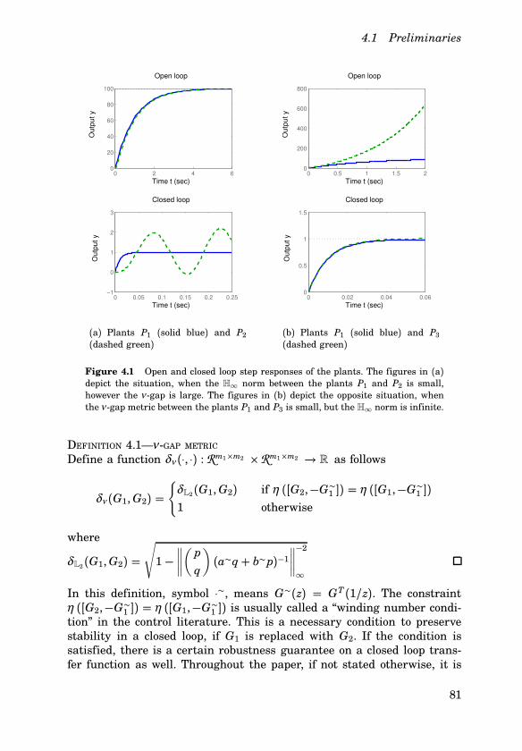
4.1 Preliminaries
0 2 4 60
20
40
60
80
100
Open loop
Time t (sec)
Outp
ut y
0 0.05 0.1 0.15 0.2 0.25−1
0
1
2
3
Closed loop
Time t (sec)
Outp
ut y
(a) Plants P1 (solid blue) and P2(dashed green)
0 0.5 1 1.5 20
200
400
600
800
Open loop
Time t (sec)
Outp
ut y
0 0.02 0.04 0.060
0.5
1
1.5
Closed loop
Time t (sec)
Outp
ut y
(b) Plants P1 (solid blue) and P3(dashed green)
Figure 4.1 Open and closed loop step responses of the plants. The figures in (a)depict the situation, when the H∞ norm between the plants P1 and P2 is small,however the ν -gap is large. The figures in (b) depict the opposite situation, whenthe ν -gap metric between the plants P1 and P3 is small, but the H∞ norm is infinite.
DEFINITION 4.1—ν -GAP METRICDefine a function δν (⋅, ⋅) : Rm1$m2 $Rm1$m2 → R as follows
δν (G1,G2) =
δL2(G1,G2) if η ([G2,−G∼1 ]) = η ([G1,−G∼1 ])
1 otherwise
where
δL2(G1,G2) =
√1−
∥∥∥∥(p
q
)(a∼q+ b∼p)−1
∥∥∥∥−2
∞
In this definition, symbol ⋅∼, means G∼(z) = GT(1/z). The constraintη ([G2,−G∼1 ]) = η ([G1,−G∼1 ]) is usually called a “winding number condi-tion” in the control literature. This is a necessary condition to preservestability in a closed loop, if G1 is replaced with G2. If the condition issatisfied, there is a certain robustness guarantee on a closed loop trans-fer function as well. Throughout the paper, if not stated otherwise, it is
81

Chapter 4. ν -gap Model Reduction
assumed that G1 and G2 are scalar, not necessarily stable, transfer func-tions. Therefore, a, b, p and q are scalar transfer functions as well.Finally, we are ready to formulate the ν -gap model reduction problem
as an optimization one. Given asymptotically stable a and b, such thatb∼b+ a∼a = 1 and b/a is not necessarily stable, solve
γ opt = minγ>0, p, q
γ (4.1)
∥∥∥∥(p
q
)(a∼q+ b∼p)−1
∥∥∥∥∞
≤ γ (4.2)
η
([p
q,−b∼
a∼
])= η
([b
a,−b∼
a∼
])(4.3)
deg(p/q) = k
Note that δν (b/a, p/q) ≤√1− 1/γ 2opt by construction. In this formulation,
b/a is a full order model, and p/q parameterizes its k-th order approxi-mation. However, the obtained program is not generally convex even forthe scalar-valued functions due to the winding number condition and thecomputation of L∞ norm. Therefore, a convexification is required.
4.2 Model Reduction in the ν -gap Metric
The program is addressed only for the discrete-time transfer functions.The continuous-time transfer functions can be discretized as in Chapter 2.There are two contributors of non-convexity in the presented formula-
tion. The first one is the L∞ norm optimization with a degree constraint,which creates a non-smooth optimization problem. Nevertheless, an effi-cient and accurate suboptimal solution may be derived using a methodfrom Chapter 2, i.e., iterative Algorithm 6 (page 48). The second one isthe winding number condition, which is much harder to address. Luckily,the techniques from Chapter 2 address the stability condition in a man-ner that can be exploited here. Therefore, only the norm constraint willbe addressed first. Then it will be shown that all the solutions of such aproblem satisfy the winding number condition.The usual approach to L∞ minimization is rewriting the constraint
(4.2) as infinite number of constraints for every frequency ω in [0,π ]:
γ 1 = minγ>0, pi, qi
γ (4.4)
∀ ω ∈ [0,π ] :
∥∥∥∥(p
q
)∥∥∥∥2
< γ pqa∼ + pb∼p
82

4.2 Model Reduction in the ν -gap Metric
where p=k∑i=0pie
−i⋅ω , q=k∑i=0qie
−i⋅ω , and qi, pi are the actual decision vari-
ables. Introduce a new variable φ into the program as:
γ 2 = minγ>0, pi, qi,φ
γ (4.5)
∀ ω ∈ [0,π ] :
∥∥∥∥(p
q
)φ∼
∥∥∥∥2
< γ Re ((qa∼ + pb∼)φ∼)
The programs (4.4) and (4.5) are equivalent, meaning that γ 1 = γ 2. Theproof of this fact is identical to the one of Lemma 2.2. It can be also shownthat an optimal choice of φ is qa∼ + pb∼. Introducing an extra variable φdoes not solve all the problems. However, by computing φ in advance andfixing it in the minimization, the program becomes quasi-convex. Given aninitial point p0 and q0, the algorithm can be iterated, with φ = q0a∼+p0b∼.The choice of the initial point is described in the sequel.Is the described set big enough to provide any improvement at all?
This question was studied in [Henrion et al., 2003] and [Yang et al., 2007],besides this thesis. The results for low orders as 2 and 3 are colorfully il-lustrated in [Henrion et al., 2003]. Given two polynomials θ and ξ thiscondition describes all positive real transfer functions with a fixed de-nominator θ . The set of all possible ξ is shown in numerical examples tobe significantly big in comparison to the set of all stable ξ . However, notheoretical results were provided in any work.By convexifying (4.2) the constraint (4.3) was incorporated into the
program. A proof of this fact is summarized in the following lemma.
LEMMA 4.1Assume that p0 and q0 are FIR filters of the same order, and b and aare asymptotically stable functions with identical poles. Assume also thatp0/q0 satisfies the winding number condition for b/a. Suppose p and q arecoprime FIR filters of the same order as p0 and q0. Let φ = q0a∼+p0b∼. IfRe ((qa∼+ pb∼)φ∼) > 0 for all the frequencies ω in [0,π ] then the windingnumber condition η ([p/q,−b∼/a∼]) = η ([b/a,−b∼/a∼]) is satisfied.
Proof. The proof is based on the proof of Lemma 2.3.Since p0/q0 satisfies the winding number condition, it is only requiredto show that η
([p0/q0,−b∼/a∼
])= η ([p/q,−b∼/a∼]). This is shown in a
straightforward manner from the condition Re ((qa∼ + pb∼)φ∼) > 0. Letc = qa∼+ pb∼, the inequality Re (cφ∼) > 0 on the unit circle is equivalentto Re (c/φ) > 0 on the unit circle. Note that the number of zeros of cand φ is equal (since the order of p, q, p0 and q0 is the same), and thepoles of c and φ are identical. Furthermore, if Re (c/φ) is positive on theunit circle, then the function c(eω )/φ(eω ) does not encircle the origin.
83

Chapter 4. ν -gap Model Reduction
Therefore, by Cauchy’s argument principle, the number of zeros and polesof c/φ inside the unit circle is equal. Since the number of zeros of c andφ is the same, it also implies that c has the same number of unstablezeros as φ . Therefore, qa∼ + pb∼ has the same number of unstable polesas q0a∼ + p0b∼, and thus η
([p0/q0,−b∼/a∼
])= η ([p/q,−b∼/a∼]) can be
verified. Finally, η ([p/q,−b∼/a∼]) = η ([b/a,−b∼/a∼]).
REMARK 4.1It is assumed that the order of q, p, q0 and p0 is the same and it is equalto k in (4.5). It is theoretically possible that the order of the obtained pand q is less than k. On the other hand in semidefinite programming,obtaining coefficients qk and pk equal to zero (which corresponds to orderk − 1) is equivalent to obtaining a matrix which is rank-deficient. Theset of rank-deficient matrices is a null measure subset of the space offull rank matrices. Therefore, it is almost improbable to obtain a rank-deficient matrix in semidefinite programming. With a similar reasoning,it can be stated that p and q are, in fact, coprime.
Finally, a quasi-convex semidefinite program for a given φ may be deduced:
γ cν = minpi, qi
γ subject to (4.6)
∀ ω ∈ [0,π ] :∥∥∥∥(p(eω )
q(eω )
)φ∼(eω )
∥∥∥∥2
< γ Re ((q(eω )a∼(eω ) + p(eω )b∼(eω ))φ∼(eω ))
THEOREM 4.1Consider the program (4.6) with a full sampling, i.e., the constraints areenforced for all the frequencies ω in [0,π ], where γ cν , p, and q is the outputof the algorithm. Then δν(G, p/q) ≤
√1− (1/γ cν )2.
Proof. Shown by construction using Lemma 4.1.
Tractable Algorithm and Implementation
The choice of the starting point is the most important part of the al-gorithm. A reasonable guideline to choose the initial point is to use anapproximation of the right NCF stacked in a vector (or the normalizedright graph symbol). A known result is used to justify such an action:
LEMMA 4.2— [VINNICOMBE, 2000]Given a plant P0 of order n
σ k ≤ infP1∈P(k)
δν (P0, P1)
84
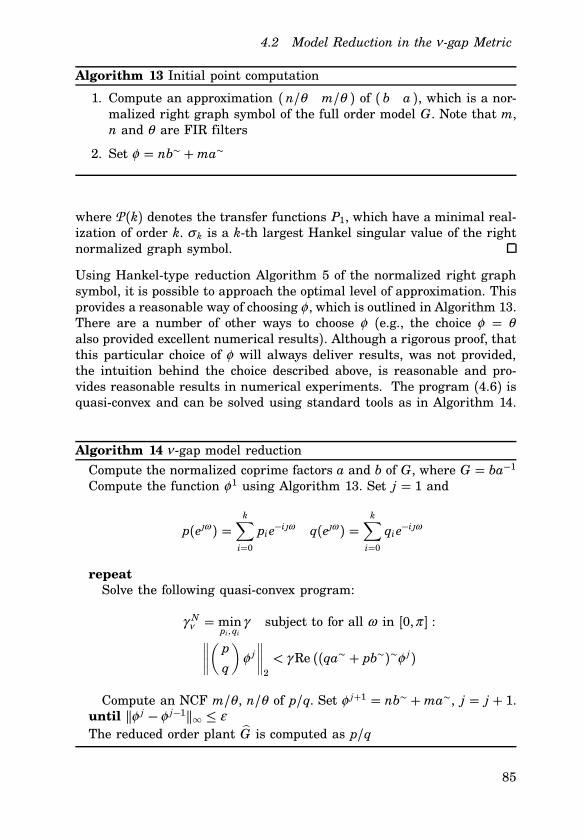
4.2 Model Reduction in the ν -gap Metric
Algorithm 13 Initial point computation
1. Compute an approximation ( n/θ m/θ ) of ( b a ), which is a nor-malized right graph symbol of the full order model G. Note that m,n and θ are FIR filters
2. Set φ = nb∼ +ma∼
where P(k) denotes the transfer functions P1, which have a minimal real-ization of order k. σ k is a k-th largest Hankel singular value of the rightnormalized graph symbol.
Using Hankel-type reduction Algorithm 5 of the normalized right graphsymbol, it is possible to approach the optimal level of approximation. Thisprovides a reasonable way of choosing φ , which is outlined in Algorithm 13.There are a number of other ways to choose φ (e.g., the choice φ = θalso provided excellent numerical results). Although a rigorous proof, thatthis particular choice of φ will always deliver results, was not provided,the intuition behind the choice described above, is reasonable and pro-vides reasonable results in numerical experiments. The program (4.6) isquasi-convex and can be solved using standard tools as in Algorithm 14.
Algorithm 14 ν -gap model reduction
Compute the normalized coprime factors a and b of G, where G = ba−1
Compute the function φ1 using Algorithm 13. Set j = 1 and
p(eω ) =
k∑
i=0
pie−iω q(eω ) =
k∑
i=0
qie−iω
repeat
Solve the following quasi-convex program:
γ Nν = minpi, qi
γ subject to for all ω in [0,π ] :∥∥∥∥(p
q
)φ j
∥∥∥∥2
< γ Re ((qa∼ + pb∼)∼φ j)
Compute an NCF m/θ , n/θ of p/q. Set φ j+1 = nb∼ +ma∼, j = j + 1.until qφ j − φ j−1q∞ ≤ ε
The reduced order plant G is computed as p/q
85
Chapter 4. ν -gap Model Reduction
The second order cone constraint can be easily transformed into a lin-ear matrix inequality (LMI) using the Schur complement, providing asemidefinite constraint instead. A frequency dependent semidefinite con-straint may be imposed for all the frequencies in [0,π ] at ones using theKalman-Yakubovitch-Popov lemma (see, Lemma 1.3). To provide a compu-tationally cheaper program the constraints may be enforced on a frequencygrid ω iNi=1, where N is big enough to avoid over-fit. The algorithm isimplemented using the interior-point solvers SEDUMI ([Sturm, 1999]) andSDPT3 ([Tütüncü et al., 1999]) and the parser YALMIP ([Löfberg, 2004])
Computational Complexity
There are two main contributors to computational complexity: computa-tion of normalized coprime factors and the optimization problem. Compu-tation of NCFs is done using Riccati equations and, therefore, complexityis O(l3) floating point operations (flops), where l is the order of the equa-tion (of the full order model G).The optimization cost of a semidefinite program differs depending on
the tolerance level, the number of decision variables and if the constraintsare enforced for all the frequencies or just on a grid. The total cost whensolved with SEDUMI does not exceed O(N21N
2.52 + N3.52 ) flops, where N1
is the number of decision variables and N2 the number of rows in theLMI constraints ([Peaucelle et al., 2002]). If constraints are enforced on afrequency grid ω iNi=1, then N1 = O(k) and N2 = N. Here, k is the orderof the approximation. In general, computing the frequency samples costsO(l3) and can be lowered to O(l log(l)) in certain cases ([Moselhy et al.,2007; Zhu et al., 2003]). If constraints are enforced using the KYP lemmafor all the frequencies in [0,π ], then N1 = O(l2) and N2 = O(l).Since the program is quasi-convex, it is solved using bisection. The tol-
erance of bisection should be higher than in the similar model reductionmethods. Low values of δν correspond to values of γ very close to 1, forinstance if δν = 0.05 then γ = 1.00125. Therefore, the tolerance of ap-proximation has to be modified accordingly depending on an application.
Multi-input-multi-output (MIMO) case
In the SISO case, a second order cone program was used, which sim-ply does not exist for matrix constraints. Therefore, another techniqueis employed. Suppose a plant with left NCF G = A−1B ∈ Rm1$m2 withA ∈ Rm1$m1 and B ∈ Rm1$m2 . Assume P, Q are the decision variablesand matrix-valued FIR filters of degree k, such that Q ∈ Rm2$m2 andP ∈ Rm1$m2 . Again, G is a full order model, and PQ−1 is a reduced orderone.
γ opt = minγ>0, Pi,Qi
γ (4.7)
86

4.2 Model Reduction in the ν -gap Metric
∥∥∥∥(P
Q
)(A∼Q + B∼P)−1
∥∥∥∥∞
≤ γ (4.8)
η([PQ−1,−A−∼B∼
])= η
([A−1B,−A−∼B∼
])(4.9)
Similarly, the condition (4.9) comes essentially for free. However, the LMI,which is obtained by enforcing the constraint for all the frequencies in[0,π ], is now more involved
P∼P+ Q∼Q ≤ γ 2(A∼Q + B∼P)∼(A∼Q + B∼P)
To address the problem, a technique introduced in [Sootla and Sou, 2010;Tobenkin et al., 2010] is used. Consider a matrix inequality (X −Y)∼(X −Y) ≥ 0, where X and Y are complex valued matrices. From this inequalityit is easy to obtain
X ∼Y + Y∼X − Y∼Y ≤ X ∼X
which is valid for arbitrary X and Y. By introducing Y - an estimate on X- the quadratic function is bounded from below and linearized. Applyingthis inequality yields the constraint
P∼P+ Q∼Q ≤ γ 2((A∼Q + B∼P)∼R+ R∼(A∼Q + B∼P) − R∼R)
which is convex and a semidefinite one is obtained using the Schur’s com-plement. In our notation, a variable R is an estimate on A∼Q + B∼P,which allows a similar iteration as in the SISO case.The winding number condition is satisfied by the same argument.
Given an appropriate frequency dependent R we have:
γ 2((A∼Q + B∼P)∼R + R∼(A∼Q + B∼P) − R∼R) ≥ P∼P+ Q∼Q ≥ 0
and thus (A∼Q + B∼P)∼R + R∼(A∼Q + B∼P) ≥ 0 for all the frequenciesω in [0,π ]. Now, a similar statement to Lemma 4.1 can be formulated andproved for Re (det(A∼Q + B∼P)∼R).To compute the initial point R0 in the MIMO case, it is required to
factorize the initial approximation G0 = P0Q−10 , where P0 and Q0 arematrix-valued FIR filters of the required order and dimensions. However,such a factorization is not always possible, to the author’s best knowl-edge. As a remedy, one can use directly the method from Chapter 2 toapproximate the normalized left graph symbol, and P0 and Q0 will beparameterized as required by default.
87
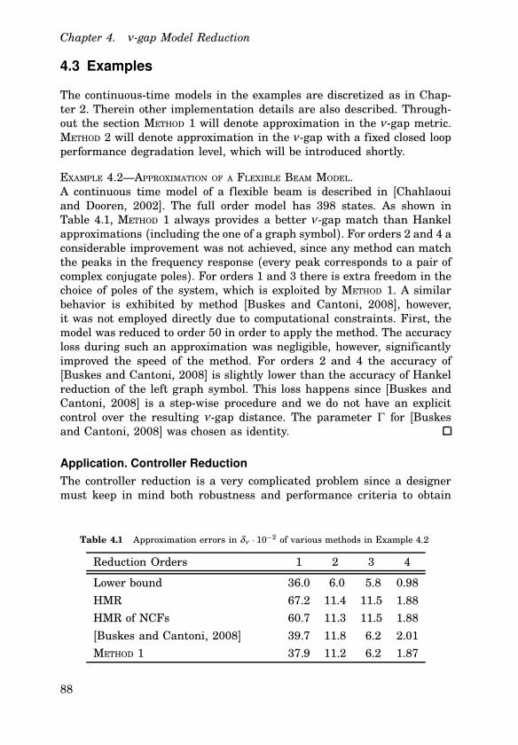
Chapter 4. ν -gap Model Reduction
4.3 Examples
The continuous-time models in the examples are discretized as in Chap-ter 2. Therein other implementation details are also described. Through-out the section METHOD 1 will denote approximation in the ν -gap metric.METHOD 2 will denote approximation in the ν -gap with a fixed closed loopperformance degradation level, which will be introduced shortly.
EXAMPLE 4.2—APPROXIMATION OF A FLEXIBLE BEAM MODEL.A continuous time model of a flexible beam is described in [Chahlaouiand Dooren, 2002]. The full order model has 398 states. As shown inTable 4.1, METHOD 1 always provides a better ν -gap match than Hankelapproximations (including the one of a graph symbol). For orders 2 and 4 aconsiderable improvement was not achieved, since any method can matchthe peaks in the frequency response (every peak corresponds to a pair ofcomplex conjugate poles). For orders 1 and 3 there is extra freedom in thechoice of poles of the system, which is exploited by METHOD 1. A similarbehavior is exhibited by method [Buskes and Cantoni, 2008], however,it was not employed directly due to computational constraints. First, themodel was reduced to order 50 in order to apply the method. The accuracyloss during such an approximation was negligible, however, significantlyimproved the speed of the method. For orders 2 and 4 the accuracy of[Buskes and Cantoni, 2008] is slightly lower than the accuracy of Hankelreduction of the left graph symbol. This loss happens since [Buskes andCantoni, 2008] is a step-wise procedure and we do not have an explicitcontrol over the resulting ν -gap distance. The parameter Γ for [Buskesand Cantoni, 2008] was chosen as identity.
Application. Controller Reduction
The controller reduction is a very complicated problem since a designermust keep in mind both robustness and performance criteria to obtain
Table 4.1 Approximation errors in δν ⋅ 10−2 of various methods in Example 4.2
Reduction Orders 1 2 3 4
Lower bound 36.0 6.0 5.8 0.98
HMR 67.2 11.4 11.5 1.88
HMR of NCFs 60.7 11.3 11.5 1.88
[Buskes and Cantoni, 2008] 39.7 11.8 6.2 2.01
METHOD 1 37.9 11.2 6.2 1.87
88
4.3 Examples
a reasonable controller. Good surveys of methods using coprime factor-ization and frequency weighted approaches, which tackle both criteriaare given in [Zhou et al., 1996] and [Obinata and Anderson, 2001]. Eventhough the performance is a robust property in the ν -gap, the metric doesnot account explicitly for the performance of the closed loop system. There-fore, it may be desirable to include the constraints on the performancelevel into the optimization problem. Using the semidefinite program as atool makes it possible. As a basis the same idea as for the ν -gap metricoptimization is employed. As an example, consider a closed loop transferfunction H(G, K ) where G is a plant and K is a controller and H is a socalled gang-of-four:
H(G, K ) =
G
1+ GK−KG
1+ GK1
1+ GK−K
1+ GK
Let b/a be an NCF of K and c/d be an NCF of G.
minγ r>0, pi, qi
γ r subject to for all ω in [0,π ]:
σ
((H(qd+ pc) −
(qc −pc
qd −pd
))ψ ∼
)< γ pRe ((qd + pc)ψ ∼)
∥∥∥∥(p
q
)φ∼
∥∥∥∥2
< γ rRe ((qa∼ + pb∼)φ∼)
where γ p is a pre-determined performance degradation level and φ is aninitial guess on qa∼ + pb∼, and ψ is an initial guess on qd+ pc. Alterna-tively, one can include a constraint on the ν -gap metric while minimizingthe performance level in the same manner.
EXAMPLE 4.3—APPROXIMATING A YOULA CONTROLLER.Consider gang-of-four H(G, K ), where the plant G is controlled in a robustmanner by a controller K . The 152-nd order controller K was obtainedin [Garpinger, 2009] using Youla parameterization. The controller itself isstable and so is the third order plant G. For every order, the level γ p willbe fixed to 75% of the performance obtained by METHOD 1. The results arepresented in Table 4.3. The parameter Γ for [Buskes and Cantoni, 2008]was chosen as identity. The method from [Buskes and Cantoni, 2008] per-forms slightly better than METHOD 1 for some orders and worse for others.However, a further extension of the approach is not easily obtainable. Butusing the presented approach it is simply a matter of adding a correspond-ing constraint.
89

Chapter 4. ν -gap Model Reduction
Table 4.2 Approximation errors of various methods in the ν -gap metric and effecton the closed loop performance in Example 4.3
Distance between K and K in the ν -gap metric (⋅10−2)
Reduction Orders 2 3 4 5 6
HMR 72.9 83.14 24.58 18.88 12.67
HMR of NCF 67.01 70.48 13.47 4.96 6.29
Lower bound 33.80 6.82 2.99 2.95 1.15
[Buskes and Cantoni, 2008] 36.68 11.54 4.69 3.25 1.70
METHOD 1 37.93 7.49 3.35 3.23 3.20
METHOD 2 44.56 7.84 4.63 4.05 4.27
Distance between H(G, K ) and H(G, K ) in H∞
Reduction Orders 2 3 4 5 6
HMR 3.64 26.02 1.09 0.84 0.35
HMR of NCF 2.37 2.34 0.92 0.34 0.38
[Buskes and Cantoni, 2008] 6.94 1.31 0.48 0.26 0.08
METHOD 1 1.92 0.58 0.27 0.26 0.26
METHOD 2 1.53 0.43 0.21 0.19 0.19
4.4 Conclusion and Discussion
A linear system approximation method in the ν -gap metric was presentedin this chapter. Such a method may be very useful for modeling of struc-tured or multi-agent systems. Approximation is obtained using semidefi-nite programming and a normalized coprime factorization of the originalmodel. This method can be applied to controller reduction by taking intoaccount the performance of a closed loop.The current algorithm has some advantages in comparison to [Buskes
and Cantoni, 2008]. Incorporating extra constraints, adding frequency-depended weights and/or restricting the objective to a specific frequencyinterval is straightforward using the frequency domain representation.However, using [Buskes and Cantoni, 2008] such extensions are not easyto obtain.
90
5
Structured Model Order
Reduction
One of the first steps to incorporate a structure into the model reductionproblem was made by [Enns, 1984]. The method extended the establishedbalanced truncation algorithm ([Moore, 1981]) to a frequency-weightedproblem. Essentially, a cascade interconnection of three systems was ap-proximated. A number of approaches to address this problem have beenproposed (e.g., [Zhou, 1995], [Sandberg and Murray, 2007]). A method re-ported by [Sandberg and Murray, 2008] can be also seen as a generalizedversion of frequency-weighted model reduction problems. An importantsubclass of systems with a structure is a controller-plant interconnection.A number of methods address the controller reduction problem includ-ing those described in [Zhou et al., 1996; Li and Paganini, 2005; Yanget al., 2007; Burke et al., 2006] and recently proposed by [Sou and Rantzer,2010b; Sou and Rantzer, 2010a].In this chapter, the focus is on an interconnection of “subsystems” in
a typical block diagram. In order to avoid any confusion the intercon-nected system will be named a “supersystem”, as opposed to subsystems.Interactions of subsystems define a certain topology of interconnectionsor a “structure” in a supersystem. Clearly, a modeling procedure shouldaccount for such a structure. Therefore, the goal of model order reduc-tion in this setting is to reduce certain subsystems, while preserving theoverall structure of the supersystem. This concept can be formalized ina concrete example. Consider two subsystems N and G interacting in alinear fractional transformation (or LFT) loop (see, [Zhou et al., 1996]).The supersystem F l (N,G) is depicted in Figure 5.1. Assume N shouldbe preserved in the reduction procedure and G should be approximatedby some G. It is also required that the resulting LFT is similar to theoriginal one, which entails that the error qF l (N,G) −F l (N, G)qH∞ hasto be minimized. However, to author’s best knowledge, there is no such
91

Chapter 5. Structured Model Order Reduction
Figure 5.1 An LFT loop with two subsystems G and N.
method, that can guarantee finding a solution for an arbitrary order ofG. Therefore, in order to simplify this problem, auxiliary input and out-put signals are introduced. By adding these signals, the transfer functionF l (N,G) will be replaced by an extended one Se(N,G), which will be, infact, reduced in the optimization problem. The extended supersystem Sedepicts the input-output mapping in Figure 5.2. Finally, the structuredmodel reduction problem is cast as a minimization one.
minlow-order G
qSe(N,G) − Se(N, G)qH∞ (5.1)
This minimization problem is approached by rewriting the system Se(N, G)in a coprime factor form. These coprime factors will also represent thestructure of interconnections. The optimization is addressed using a two-step procedure employed in different fixed order controller design methods(see, [Apkarian and Noll, 2006; Arzelier et al., 2010] and the referencestherein). In such a procedure, first a stabilizing plant is obtained andthen the performance is minimized. The LFT case is discussed in detailin Section 5.1.In Section 5.2, the reduction of multiple subsystems is discussed. An
LFT loop is replaced by an arbitrary block diagram, with multiple sub-systems interacting with each other. Finally, numerical examples are pre-sented in Section 5.3.
y
z1
z2
= Se(N,G)
u
w1
w2
Figure 5.2 An extended supersystem Se with two subsystems G and N.
92

5.1 Model Reduction in an LFT loop
5.1 Model Reduction in an LFT loop
Consider an LFT loop in Figure 5.2 and the minimization criterion (5.1).The biggest advantage of introducing the auxiliary signals wi and zi isthe ability to create a convenient coprime factor representation. This rep-resentation is computed by a direct calculation using the coprime factor-ization of N and G. Indeed, the extended system Se can be described bythe following set of equations:
[y
z1
]=
[N11 N12
N21 N22
] [u
z2 +w1
]
z2 = G(w2 + z1)
Factorize N and G using a left coprime factorization, i.e.:[N11 N12
N21 N22
]=
[QN11 QN12
QN21 QN22
]−1 [PN11 PN12
PN21 PN22
]
G = Q−1G PG
and substitute them into the equations above:[QN11 QN12
QN21 QN22
] [y
z1
]=
[PN11 PN12
PN21 PN22
] [u
z2 +w1
]
QG z2 = PG(w2 + z1)
Since z1 and z2 are treated as outputs, they are moved to the left handside of the equations
[QN11 QN12 −PN12
QN21 QN22 −PN22
]y
z1
z2
=
[PN11 PN12
PN21 PN22
] [u
w1
]
−PG z1 + QG z2 = PGw2
Both equations can be united into the following matrix equationQN11 QN12 −PN12
QN21 QN22 −PN22
0 −PG QG
y
z1
z2
=
PN11 PN12 0
PN21 PN22 0
0 0 PG
u
w1
w2
Finally, define the transfer matrices P and Q as follows.
P =
PN11 PN12 0
PN21 PN22 0
0 0 PG
Q =
QN11 QN12 −PN12
QN21 QN22 −PN22
0 −PG QG
93
Chapter 5. Structured Model Order Reduction
LEMMA 5.1The transfer matrices P and Q are left coprime over H∞.
Proof. To show coprimeness, the definition from [Zhou et al., 1996] isused: transfer matrices P and Q are left coprime in H∞ if there existrational transfer matrices X and Y in H∞ such that
P ⋅ X +Q ⋅ Y = I
Due to coprimeness of PN and QN , there exist such XNii and YNii that
(PN11 PN12
PN21 PN22
)(XN11 XN12
XN21 XN22
)+
(QN11 QN12
QN21 QN22
)(YN11 YN12
YN21 YN22
)= I
similarly XG and YG are defined trough PG and QG
PGXG + QGYG = I
To prove coprimeness of P and Q , the transfer matrices X and Y can bechosen as
X =
XN11 XN12 0
XN21 XN22 YG
YN21 YN22 XG
Y =
YN11 YN12 0
YN21 YN22 0
0 0 YG
Finally, the relation PX +QY = I is verified by direct computation.Now examine the transfer matrices P andQ closely. Every block-row of
each transfer matrix depends either on a coprime factor of N, either on acoprime factor of G. It can not be called a “sparsity structure”, since someentries are repeated in P and Q , however, this kind of structure can beexploited by iterative Algorithm 6 on page 48. Note also that Se is stableif and only if Q has a stable inverse.
REMARK 5.1The state-space representation also manifests the structure in a conve-nient manner. Assume the space-space representations of N and G aregiven as follows.
N =
AN BN1 BN2
CN1 DN11 DN21
CN2 DN21 DN22
G =
[AG BG
CG DG
](5.2)
94

5.1 Model Reduction in an LFT loop
where DG is set to 0, which is a common assumption in control theory. Toshorten the notation, additionally define
BN = [ BN1 BN2 ] DN =
[DN11 DN12
DN21 DN22
]CN =
[CN1
CN2
]
A state space representation can be derived for P and Q
[P Q ] =
AN + LNCN 0 BN + LNDN 0 LN −BN2
0 AG + LGCG 0 BG [ 0 −BG ] LG
CN 0 DN 0 I 0
0 CG 0 0 0 I
where LN and LG are free parameters, which are used to stabilize thecoprime factors. The dynamics of the subsystems N and G are completelydecoupled. The structure manifests itself only in the input and output ma-trices. If model reduction in the time domain is considered, the transferfunction [P Q ] can be approximated using a structured Gramian frame-work from [Sandberg and Murray, 2008]. However, stability of Se(N, G)is achieved if the reduced order Q has a stable inverse. This propertyis generally hard to accommodate. Also in the presented examples, thisapproach reduces to known coprime factor reduction techniques. Due tothese reasons, this approach is not currently investigated.
Analysis of the Problem Formulation
Above, instead of solving
argminlow-order G
qF l (N,G) −F l (N, G)qH∞ (5.3)
it is proposed to address the following optimization problem
argminlow-order G
qSe(N,G) − Se(N, G)qH∞ (5.4)
The major feature in (5.4) is the ability of tracking signals wi and zi. Itmeans that not only the behaviour of F l is approximated as in (5.3), butalso the interaction between N and G.
95
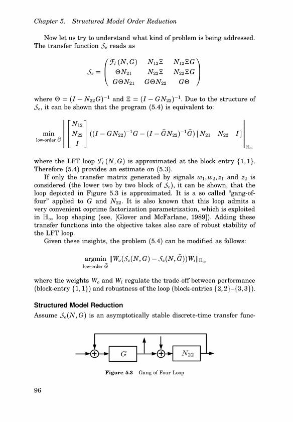
Chapter 5. Structured Model Order Reduction
Now let us try to understand what kind of problem is being addressed.The transfer function Se reads as
Se =
F l (N,G) N12Ξ N12ΞG
ΘN21 N22Ξ N22ΞG
GΘN21 GΘN22 GΘ
where Θ = (I − N22G)−1 and Ξ = (I − GN22)
−1. Due to the structure ofSe, it can be shown that the program (5.4) is equivalent to:
minlow-order G
∥∥∥∥∥∥∥
N12
N22
I
((I − GN22)−1G − (I − GN22)−1G) [ N21 N22 I ]
∥∥∥∥∥∥∥H∞
where the LFT loop F l (N,G) is approximated at the block entry 1, 1.Therefore (5.4) provides an estimate on (5.3).If only the transfer matrix generated by signals w1,w2, z1 and z2 is
considered (the lower two by two block of Se), it can be shown, that theloop depicted in Figure 5.3 is approximated. It is a so called “gang-of-four” applied to G and N22. It is also known that this loop admits avery convenient coprime factorization parametrization, which is exploitedin H∞ loop shaping (see, [Glover and McFarlane, 1989]). Adding thesetransfer functions into the objective takes also care of robust stability ofthe LFT loop.Given these insights, the problem (5.4) can be modified as follows:
argminlow-order G
qWo(Se(N,G) − Se(N, G))WiqH∞
where the weights Wo and Wi regulate the trade-off between performance(block-entry 1, 1) and robustness of the loop (block-entries 2, 2–3, 3).
Structured Model Reduction
Assume Se(N,G) is an asymptotically stable discrete-time transfer func-
Figure 5.3 Gang of Four Loop
96
5.1 Model Reduction in an LFT loop
tion. The H∞ optimization problem being addressed reads as
minP ,Q
qSe(N,G) −Q−1PqH∞
subject to: Q has a stable inverse(5.5)
where Q and P correspond to the left coprime factorization of Se(N, G) =Q−1P and G is a low order approximation of G. The reduction procedurewill be decoupled into two problems: finding a stability preserving low-order approximation of G by some G0 without considering the quality ofthe loop Se(N, G0). There are quite a few reduction techniques of struc-tured models which guarantee stability under certain conditions. However,none of those can guarantee finding a solution, if one exists. Given thisinitial point G0, the approximation quality of (5.5) is minimized.Let us return to the problem at hand: (5.5). The transfer matrices Q
and P admit the following structure:
P =
PN11 PN12 0
PN21 PN22 0
0 0 Y
Q =
QN11 QN12 −PN12
QN21 QN22 −PN22
0 −Y X
where
N =
[N11 N12
N21 N22
]=
[QN11 QN12
QN21 QN22
]−1 [PN11 PN12
PN21 PN22
]
and unknown functions are parameterized as
X =
r∑
i=0
X iz−i Y =
r∑
i=0
Yiz−i
with the real matrices X i,Yi being the decision variables. The transfermatrices X and Y constitute a left coprime factorization of G = X −1Y.To address this problem, rewrite it with an infinite number of con-
straints as in Chapter 2. For brevity, let Se = Se(N,G), and assume thatQ and P are our decision variables.
minQ,P ,γ
γ 2 subject to: Q has a stable inverse
(Se −Q−1P)(Se −Q
−1P)∼ ≤ γ 2 I ∀ω ∈ [0,π ]
where Q∼(z) = QT(1/z). For the moment, consider only the norm con-straint, which using algebraic manipulations yields:
(QSe −P)(QSe −P)∼ ≤ γ 2QQ∼ ∀ω ∈ [0,π ]
97
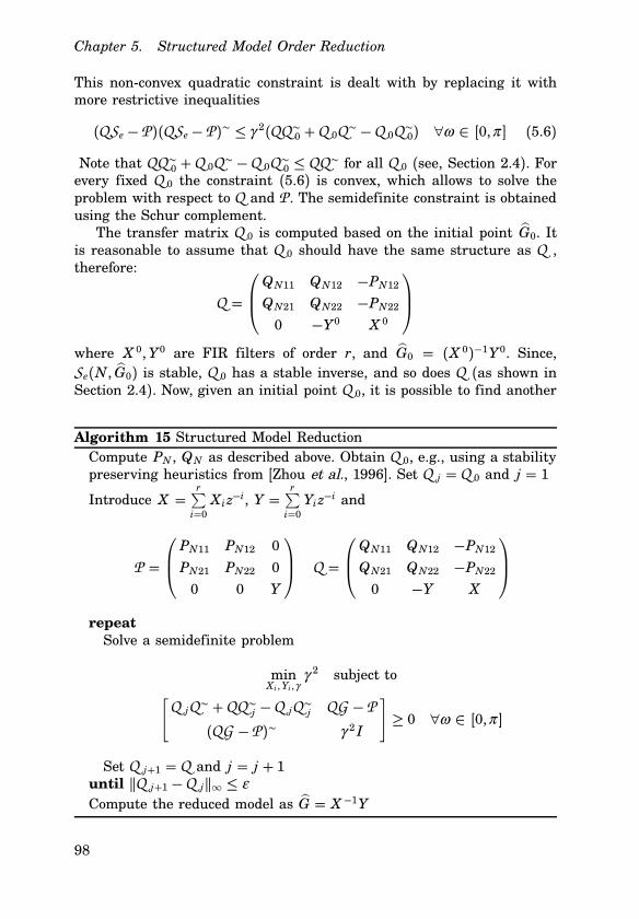
Chapter 5. Structured Model Order Reduction
This non-convex quadratic constraint is dealt with by replacing it withmore restrictive inequalities
(QSe −P)(QSe −P)∼ ≤ γ 2(QQ∼0 +Q 0Q
∼ −Q 0Q∼0) ∀ω ∈ [0,π ] (5.6)
Note that QQ∼0 +Q 0Q∼ −Q 0Q∼0 ≤ QQ
∼ for all Q 0 (see, Section 2.4). Forevery fixed Q 0 the constraint (5.6) is convex, which allows to solve theproblem with respect to Q and P . The semidefinite constraint is obtainedusing the Schur complement.The transfer matrix Q 0 is computed based on the initial point G0. It
is reasonable to assume that Q 0 should have the same structure as Q ,therefore:
Q =
QN11 QN12 −PN12
QN21 QN22 −PN22
0 −Y0 X 0
where X 0,Y0 are FIR filters of order r, and G0 = (X 0)−1Y0. Since,Se(N, G0) is stable, Q 0 has a stable inverse, and so does Q (as shown inSection 2.4). Now, given an initial point Q 0, it is possible to find another
Algorithm 15 Structured Model ReductionCompute PN , QN as described above. Obtain Q 0, e.g., using a stabilitypreserving heuristics from [Zhou et al., 1996]. Set Q j =Q 0 and j = 1
Introduce X =r∑i=0X iz
−i, Y =r∑i=0Yiz
−i and
P =
PN11 PN12 0
PN21 PN22 0
0 0 Y
Q =
QN11 QN12 −PN12
QN21 QN22 −PN22
0 −Y X
repeat
Solve a semidefinite problem
minX i,Yi,γ
γ 2 subject to[Q jQ∼ +QQ∼j −Q jQ
∼j QG −P
(QG −P)∼ γ 2 I
]≥ 0 ∀ω ∈ [0,π ]
Set Q j+1 = Q and j = j + 1until qQ j+1 −Q jq∞ ≤ ε
Compute the reduced model as G = X −1Y
98
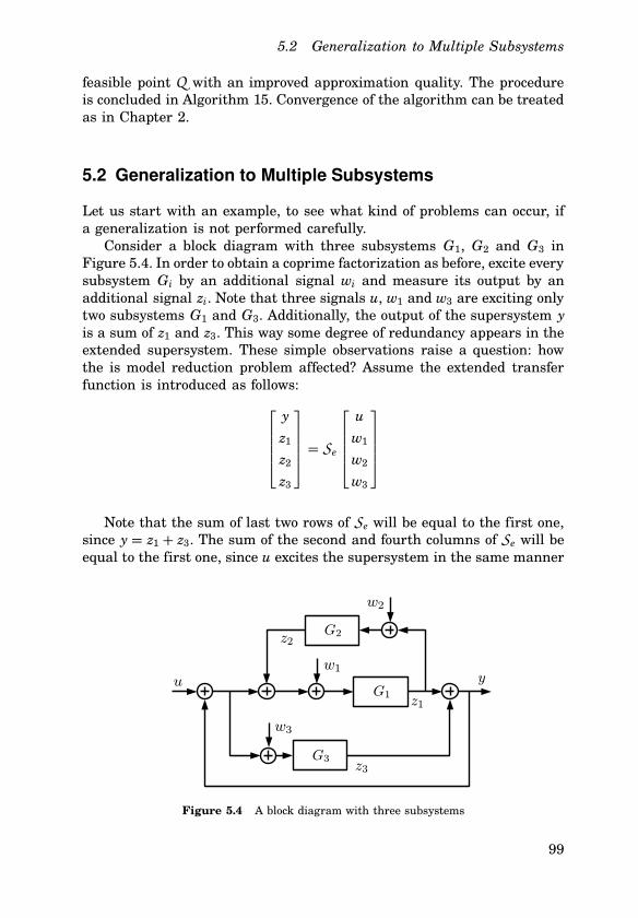
5.2 Generalization to Multiple Subsystems
feasible point Q with an improved approximation quality. The procedureis concluded in Algorithm 15. Convergence of the algorithm can be treatedas in Chapter 2.
5.2 Generalization to Multiple Subsystems
Let us start with an example, to see what kind of problems can occur, ifa generalization is not performed carefully.Consider a block diagram with three subsystems G1, G2 and G3 in
Figure 5.4. In order to obtain a coprime factorization as before, excite everysubsystem Gi by an additional signal wi and measure its output by anadditional signal zi. Note that three signals u, w1 and w3 are exciting onlytwo subsystems G1 and G3. Additionally, the output of the supersystem yis a sum of z1 and z3. This way some degree of redundancy appears in theextended supersystem. These simple observations raise a question: howthe is model reduction problem affected? Assume the extended transferfunction is introduced as follows:
y
z1
z2
z3
= Se
u
w1
w2
w3
Note that the sum of last two rows of Se will be equal to the first one,since y = z1 + z3. The sum of the second and fourth columns of Se will beequal to the first one, since u excites the supersystem in the same manner
Figure 5.4 A block diagram with three subsystems
99

Chapter 5. Structured Model Order Reduction
as the sum of w1 and w3. Thus, the transfer matrix Se will have at leastone zero singular value for all the frequencies ω in [0,π ]. Solving a modelreduction problem in this setting is problematic, since a rank-deficientmatrix is approximated. On the other hand, all zero singular values canbe eliminated while designing the extended supersystem. Therefore, somesignals should be eliminated to provide a full rank Se for all the frequen-cies. Here, signals z1 and w3 were chosen to be eliminated, providing theequations:
y = z3 + G1(u+ y+w1 + z2)
z2 = G2(w2 + y− z3)
z3 = G3(u+ y)
Factorize the subsystems Gi using left coprime factorizations Q−1i Pi. Sub-stitute them into the equations above, while multiplying both sides withQi. Also, separate the outputs and inputs on the different sides of theequations:
(Q1 − P1)y+ P1z2 − Q1z3 = P1(u+w1)
−P2y+ Q2z2 + P2z3 = P2w2
−P3y+ Q3z3 = P3u
The relationship between the signals can be computed as:
Q1 − P1 P1 −Q1
−P2 Q2 P2
−P3 0 Q3
y
z2
z3
=
P1 0 P1
0 P2 0
0 0 P3
w1
w2
u
This representation is left coprime, to show this let:
P =
P1 0 P1
0 P2 0
0 0 P3
Q =
Q1 − P1 −P2 −Q1
−P2 Q2 P2
−P3 0 Q3
PG =
P1 0 0
0 P2 0
0 0 P3
Q G =
Q1 0 0
0 Q2 0
0 0 Q3
Given the notations, it can be computed that
[P Q ] = [PG Q G ]T
where the transformation T is invertible. Note that PG and Q G are leftcoprime, since they are block diagonal with left coprime factors of the
100
5.2 Generalization to Multiple Subsystems
Algorithm 16 Coprime factorization of an arbitrary block diagram
• Given a block diagram with interconnected subsystems G1, G2, . . . ,Gn, introduce signals wi, zi. Every wi excites the subsystem Gi, andevery zi measures its output
• If u excites the system Se the same way as a linear combination ofwj , then one of the signals wj is set to zero
• If a signal zj is a linear combination of other output signals it iseliminated by zj = y−
∑nj ,=i γ j zj , where γ j are zeros or ones
• Write down the equations describing dependence of zi on the signalswj , u, y and zj , while replacing Gi by its left coprime factorizationQ−1i Pi
• Compute the left coprime factors P and Q
block diagonal and there exist XG and YG such that:
[PG Q G ]
[XG
YG
]= I
Thus, there exist stable X and Y such that:
[P Q ]
[X
Y
]= I where
[X
Y
]= T−1
[XG
YG
]
This proves that P and Q are left coprime if and only if PG and Q G areleft coprime.Inspired by this simple example, Algorithm 16 is formulated. The algo-
rithm is constructive, however, it has to be shown that it always producesa left coprime factorization.
LEMMA 5.2The transfer matrices P and Q obtained in Algorithm 16 are left coprime.
Proof. The proof is a generalization of the technique described for theblock diagram investigated above. Introduce PG and Q G :
PG =
P1 0
. . .
0 Pn
QG =
Q1 0. . .
0 Qn
101

Chapter 5. Structured Model Order Reduction
where Qi and Pi are left coprime and Gi = Q−1i Pi. The equations describ-ing the relationships between the signals read as:
Qizi = Pi(αi0u +α iwi + β i0y+
n∑
j=1
β ij zj) or
Qi(y−
n∑
j ,=i
γ j zj) = Pi(αi0u+α iwi + β i0y+
n∑
j=1
β ij zj)
where α i0,α i, β ij and γ j are equal to zero or one, depending on a particularblock diagram. The lower case appears when a signal zi is a linear combi-nation of other outputs, i.e., zi = y−
∑nj ,=i γ j zj , and it is eliminated. Note
that P will not depend onQ G since none of the signals u, wi are multipliedwith Qi. The static transformation between the transfer matrices PG , Q Gand P , Q are given as follows.
[P Q ] = [PG Q G ]
[T11 T12
0 T22
]
Since the transformation is block triangular, it remains to show that T11and T22 are invertible. For most of the signals, we have
Qizi = Pi(αi0u +α iwi + β i0y+
n∑
j=1
β ij zj)
The transfer matrix Q GT22 will be affected only by the summands con-taining multiplication of Qi and the outputs y or zi. Therefore, most ofthe block rows of Q GT22 will have only one non-zero entry Qi and it willappear on the block diagonal. For a single equation we have:
Qi(y−
n∑
j ,=i
γ j zj) = Pi(αi0u+α iwi + β i0y+
n∑
j=2i
β ij zj)
and therefore one block row ofQ GT22 consists of multiple Qi with differentsigns. Without loss of generality, we can assume that zi with i = 1 iseliminated, therefore T22 is a block-triangular matrix with the identitymatrices on the block diagonal. Only the first block row has non-zero offdiagonal entries. Given these facts T22 is invertible.It can be similarly shown that T11 is an invertible block-triangular
matrix, where only one block-column has non-zero entries except for theblock-diagonal elements. Since T11 and T22 are invertible so is the whole
102
5.3 Examples
transformation. Due to coprimeness of PG and Q G , there exist XG andYG such that:
[PG Q G ]
[XG
YG
]= I
Finally, there exist stable X and Y such that
[P Q ]
[X
Y
]= I where
[X
Y
]=
[T11 T12
0 T22
]−1 [XG
YG
]
Therefore P and Q are left coprime if and only if PG and Q G are leftcoprime, which is satisfied by construction.The statement of this lemma is not unexpected. If there is just one
subsystem with one input and one output, then the coprime factors P ,Q should have one input and one output. It stands to reason that theextended supersystem Se should have n inputs and n outputs, if there isn subsystems in Se with one input and one output each. Stability of thesupersystem is equivalent to Q and Q−1 being stable, since the transfermatrices P and Q constitute a coprime factorization of Se.Addressing the model reduction problem can be done similarly as was
done before. Assume without loss of generality, that subsystems Gk+1, . . . ,Gnhave to be preserved during the approximation procedure and G1, . . . ,Gkare being reduced. All the subsystems Gk+1, . . . ,Gn are treated as onesubsystem N and the problem is cast a minimization one as follows.
minlow order G1 ,...,Gk
qSe(N,G1, . . . ,Gk) − Se(N, G1, . . . , Gk)qH∞
After that, Algorithm 6 can be modified in a straightforward manner inorder to address this problem.
5.3 Examples
All the algorithms are implemented using SEDUMI ([Sturm, 1999]) andYALMIP ([Löfberg, 2004]). The first example depicts a continuous timeclosed loop. Therefore, the model is discretized as in Chapter 2.
EXAMPLE 5.1—CONTROLLER REDUCTION IN THE LFT STRUCTUREConsider an LFT structure F l (G, K ) as in Figure 5.5 with G being aplant and K a controller, which is desirable to reduce. The structured leftcoprime factorization is computed as follows.
P =
PG11 PG12 0
PG21 PG22 0
0 0 PK
Q =
QG11 QG12 −PG12QG21 QG22 −PG220 −PK QK
103

Chapter 5. Structured Model Order Reduction
Figure 5.5 LFT structure
Table 5.1 Approximation errors qFl(G, K ) −Fl(G, K )qH∞ in Example 5.1
Reduction Orders 2 3 4 5 6 7
SWA SHMR 2.75 0.69 0.42 0.34 0.19 0.22
ALG 15 0.98 0.68 0.34 0.31 0.17 0.14
The reduction techniques were tested on the famous example by Enns,which was a model reduction case study in [Zhou et al., 1996]. The initialpoint computation is performed by using SWA method (see, [Zhou et al.,1996]), which can be formulated as follows:
minK
∥∥∥Wa(K − K )∥∥∥H∞
where Wa = (I − G22K )−1G22
The problem was addressed by frequency-weighted semidefinite Hankel-type model reduction (see, Chapter 2). ALG 15 will denote Algorithm 15with the result of SWA SHMR as a starting point.Table 5.1 shows that the improvement in the approximation error be-
tween the original and the reduced models is noticeable almost for everyorder. Table 5.2 shows that the performance of ALG 15 is near the originalone qF l(G, K )qH∞ = 1.2 for orders 4− 7. For order 2 ALG 15 outperformedSWA considerably. In fact, even performance oriented methods PWRCFand PWA by [Zhou et al., 1996] can not achieve such performance levels.
EXAMPLE 5.2—MIXED SENSITIVITY CONTROL LOOPConsider a structure as in Figure 5.6, where K is a controller and G is aplant. Notice that in this example there is no need to add extra inputs andoutputs. The left coprime factorization of this supersystem is as follows:
P =
[PG 0
0 PK
]Q =
[QG −PG
−PK QK
]
104

5.3 Examples
Table 5.2 Performance of the reduced closed loop qFl(G, K )qH∞ in Example 5.1
Reduction Orders 2 3 4 5 6 7
SWA SHMR 3.44 1.65 1.34 1.29 1.23 1.23
PWRCF H/O 1.98 2.03 1.19 1.19 1.19 1.19
PWA H/O 1.94 2.73 1.19 1.19 1.19 1.19
ALG 15 1.34 1.34 1.21 1.23 1.20 1.20
Table 5.3 Approximation errors qSe(G, K ) − Se(G, K )qH∞ in Example 5.2
Reduction Orders 2 3 4 5 6 7 8
SWA SHMR 0.91 0.39 0.13 0.14 0.04 0.04 0.04
ALG 15 0.63 0.07 0.06 0.04 0.01 0.01 0.01
where K = Q−1K PK and G = Q−1G PG . In this subsection a similar notation
and methods will be used. However, the weight in SWA is changed to:
Wa =
[G
I
](I + KG)−1
ALG 15 will denote Algorithm 15 with a starting point from SWA SHMR.The controller was designed by [Garpinger, 2009]. The plant is asymp-
totically stable with poles near the imaginary axis. This makes the sta-bilization almost redundant, requiring only the performance level to beoptimized.As seen from Table 5.3 the approximation errors are significantly
improved by the proposed approach in comparison to SWA. However, itshould be noted that, since the plant is stable, the problem for the fixed-order controller design is much easier than in Example 5.1, for instance.Table 5.4 shows, that the performance levels of ALG 15 is always within10% of the nominal value qSe(G, K )qH∞ = 1. The improvement in approx-imation error is quite remarkable when comparing ALG 15 to SWA.
Figure 5.6 Mixed Sensitivity Control loop
105

Chapter 5. Structured Model Order Reduction
Table 5.4 Performance of the closed loop qSe(G, K )qH∞ in Example 5.2
Reduction Orders 2 3 4 5 6 7 8
SWA SHMR 1.38 1.15 0.87 0.87 0.99 0.98 0.98
ALG 15 1.11 0.93 0.94 0.95 1.00 1.01 1.01
5.4 Conclusion and Discussion
A few generalizations of known results are described in this chapter. Forinstance, a coprime factorization of structured systems is introduced, aknown two-step procedure is generalized to an arbitrary supersystem andessentially any number of subsystems. There are a few issues which arestill not addressed in this thesis and require further research.
• Is it possible to generalize the normalized coprime factorizations tothe structured case? In the current setting it is not clear how thisgeneralization may occur. Perhaps instead of a direct generalizationto supersystems, one can normalize the factors of subsystems.
• The problem of computing an initial point is crucial for this ap-proach. However, to the author’s best knowledge, it is a commonproblem in all the methods unless a special type of system is be-ing reduced, such as a positive, positive-real system. Nevertheless,a number of methods can obtain an initial point in a heuristic man-ner and using the presented framework it is possible to considerablyimprove the quality of approximation.
• There are similar two-step procedures, which can be used to addressthe model reduction problem. One such method addresses the non-smooth optimization problem directly ([Apkarian and Noll, 2006]).The comparison of the proposed approach to [Apkarian and Noll,2006] is a topic of future research.
106

6
Conclusion and Discussion
6.1 Summary of Thesis
The main contribution of this thesis is the development of two modelreduction methods. Both methods are based on matching of the frequencyresponse samples of the full and reduced order models. This approach iscomputationally cheap for a certain class of models. Both methods alsoguarantee stability. If required, a number of extensions can be performedas well, such as frequency-weighting, enforcing passivity and so on.The first method is based on a relaxation approach, which results in
semidefinite Hankel-type model reduction (SHMR). Due to significant re-semblance to optimal Hankel model reduction, the accuracy of SHMR isvery similar to the Hankel model reduction one. It can be argued thatSHMR is a numerically scalable approach to Hankel model reduction.The SHMR algorithm can be applied to H∞ model reduction and para-meterized model reduction problems, which are described in chapters 2and 3. However, in the second case, explicit parameter-dependent modelsare not easily obtainable. In both H∞ and parameterized model reductionproblems the relaxation gap is estimated, which acts as lower and uppererror bounds on the approximation error. Although the upper bounds arevery conservative, estimation of a relaxation gap is required to motivatethe relaxation.The second method constitutes an iterative approach, where on every
iteration a semidefinite program has to be solved. This method can beapplied to all the problems described in the thesis: H∞ model reduction,parameterized model reduction, ν -gap model reduction and, finally, struc-tured model reduction. The major issue of the method is the computationof the initial point of the algorithm. In H∞ model reduction computation ofinitial point is rather straightforward. One can also be computed based on
107
Chapter 6. Conclusion and Discussion
the approximation computed by another model reduction method. There-fore, the iterative approach can potentially improve the quality of anymodel reduction method. In parameterized and ν -gap model reductionthe computation of an initial point is more involved, but always feasible.A few guidelines is provided for a reasonable computation of the initialpoint. However, in structured model reduction computation of the initialpoint is an open question. In this thesis, such computation was not theforemost goal and a few known heuristics were listed, which address thisproblem.The iterative approach is, essentially, addressing a non-smooth, non-
convex optimization problem. Therefore, it is hard to theoretically predictthe properties of the resulting solution. Nonetheless, the numerical sim-ulations show promising results with respect to accuracy of the iterativeapproach.
6.2 Discussion on Future Work
There are a few open questions concerning the presented framework. Someof the questions are well known in the control literature. For example,computation of the initial point in structured model reduction is relatedto fixed order controller design and static output feedback problem. Theseproblems are known to be hard and all the solutions are yet to be found.Other questions arose with the development of the methods in this thesis.These are discussed in detail.
Properties of the Iterative Approach
The iterative approach is a powerful tool to address the model reduc-tion problem. It was shown that the limit point always exists, however,the properties of this limit point seem hard to investigate. Due to non-convexity of the objective function, it is certainly possible to obtain a limitpoint, which is not equal to the global minimizer. The relaxation approach(the SHMR method) guarantees a certain sub-optimality and a solutionthat is relatively close to the global minimum in terms of the objectivefunction. However, there is no guarantee that minimizer of the relaxedproblem is also close to the global minimizer. The main obstacle in evalu-ation of the obtained minimizer is lack of properties of a globally optimalsolution. To author’s best knowledge, there is no known results concern-ing the optimal solutions in H∞ model reduction, which is a non-smoothoptimization problem.A certain analogue to the iterative method can be obtained for the
H2 model reduction problem for which conditions for local optimality are
108

6.2 Discussion on Future Work
known. Therefore, one of the future work directions will be evaluation ofsuch a method. Such an evaluation can shed light on H∞ problem as well.
Applications of Parameterized Model Order Reduction Framework
The presented parameterized model order reduction method performs ex-tremely well when the parameters in the model are constant. When theLPV systems are considered, the picture is not as clear. One problem isstability, since only a necessary condition is guaranteed.Even if stability can be addressed, a problem occurs in accuracy of ap-
proximation. Consider the variables ω and θ used in the presented algo-rithms. Here ω is a frequency variable, and θ is a parameter. Throughoutthe derivation of the algorithms, it is assumed that ω and θ are inde-pendent. However, in practice, the parameter θ does depend on time andstates and, therefore, it depends on ω . It means that inactive modes ofθ are kept, which creates conservatism. One possibility to reduce conser-vatism, is using frequency weights in order to get a better match alongsome frequencies. However, it is not clear at this point how determinethese weights and if this approach is valid at all.
109

7
Bibliography
Anderson, B. and A. C. Antoulas (1986): “On the scalar rational interpo-lation problem.” In Hinrichsen and Willems, Eds., IMA J. of Math-ematical Control and Information, Special Issue on Parametrizationproblems, vol. 3, pp. pp. 61–88. Oxford University Press.
Antoulas, A. (2009): “An overview of model reduction methods and a newresult.” In Proceedings of 48th Conference on Decision and Control,pp. 5357–5362. Shanghai, PRC.
Antoulas, A. C. (2005): Approximation of Large-Scale Dynamical Systems(Advances in Design and Control). Society for Industrial and AppliedMathematics, Philadelphia, PA, USA.
Antoulas, A. C., D. C. Sorensen, and S. Gugercin (2001): “A surveyof model reduction methods for large-scale systems.” ContemporaryMathematics, 280, pp. 193–219.
Apkarian, P. and D. Noll (2006): “Nonsmooth H-infinity synthesis.”Automatic Control, IEEE Transactions on, 51:1, pp. 71 – 86.
Arzelier, D., E. N. Gryazina, D. Peaucelle, and B. T. Polyak (2010): “Mixedlmi/randomized methods for static output feedback control design.” InAmerican Control Conference (ACC), 2010, pp. 4683 –4688.
Åström, K. J. and R. M. Murray (2008): Feedback Systems: An Introduc-tion for Scientists and Engineers. Princeton University Press, Prince-ton, NJ, USA.
Beck, C., J. Doyle, and K. Glover (1995): “Model reduction of multi-dimensional and uncertain systems.” IEEE Transactions on AutomaticControl, 41, pp. 1466–1477.
Bond, B. and L. Daniel (2005): “Parameterized model order reductionof nonlinear dynamical systems.” In ICCAD ’05: Proceedings of the
110

2005 IEEE/ACM International conference on Computer-aided design,pp. 487–494. IEEE Computer Society, Washington, DC, USA.
Bongers, P. and P. Heuberger (1990): “Discrete normalized coprime factor-ization.” In Bensoussan and Lions, Eds., Analysis and Optimization ofSystes, vol. 144 of Lecture Notes in Control and Information Sciences,pp. 307–313. Springer Berlin / Heidelberg.
Boyd, S. and L. Vandenberghe (2004): Convex Optimization. CambridgeUniversity Press.
Burke, J. V., D. Henrion, A. S. Lewis, and M. L. Overton (2006): “HIFOO- a MATLAB package for fixed-order controller design and H-infinityoptimization.” In IFAC Symposium on Robust Control Design Toulouse.France.
Buskes, G. and M. Cantoni (2007): “Reduced order approximation in theν -gap metric.” In Decision and Control, 2007 46th IEEE Conferenceon, pp. 4367 –4372.
Buskes, G. and M. Cantoni (2008): “A step-wise procedure for reducedorder approximation in the ν -gap metric.” In Decision and Control,2008. CDC 2008. 47th IEEE Conference on, pp. 4855 –4860.
Cantoni, M. (2001): “On model reduction in the ν -gap metric.” In Decisionand Control, 2001. Proceedings of the 40th IEEE Conference on, vol. 4,pp. 3665 –3670 vol.4.
Chahlaoui, Y. and P. V. Dooren (2002): “A collection of benchmarkexamples for model reduction of linear time invariant dynamicalsystems.” SLICOT Working Note 2002-2. Univesité Catholique deLouvain.
Daniel, L., C. S. Ong, S. C. Low, K. H. Lee, and J. White (2002): “Geometri-cally parameterized interconnect performance models for interconnectsynthesis.” In ISPD ’02: Proceedings of the 2002 international sympo-sium on Physical design, pp. 202–207. ACM, New York, NY, USA.
Daniel, L., O. Siong, L. Chay, K. Lee, and J. White (2004): “Multiparam-eter moment matching model reduction approach for generating geo-metrically parameterized interconnect performance models.” Trans. onComputer Aided Design of Integrated Circuits, 23:5, pp. 678–93.
Daniel, L. and J. White (2003): “Automatic generation of geometrically pa-rameterized reduced order models for integrated spiral RF-inductors.”In International Workshop on Behavioral Modeling and Simulation,pp. 18–23. IEEE.
111

Chapter 7. Bibliography
Dritschel, M. A. and H. J. Woerdeman (2005): “Outer factorizations in oneand several variables.” Transactions of the American MathematicalSociety, 357:11.
Dumitrescu, B. (2007): Positive Trigonometric Polynomials and SignalProcessing Applications. Dordrecht, The Netherlands:Springer-Verlag.
Ekstrom, M. and J. Woods (1976): “Two-dimensional spectral factorizationwith applications in recursive digital filtering.” Acoustics, Speech andSignal Processing, IEEE Transactions on, 24:2, pp. 115–128.
Enns, D. F. (1984): “Model reduction with balanced realizations: An errorbound and a frequency weighted generalization.” Decision and Control,1984. The 23rd IEEE Conference on, 23, Dec., pp. 127–132.
Fairman, F., G. Danylchuk, J. Louie, and C. Zarowski (1992): “A state-space approach to discrete-time spectral factorization.” Circuits andSystems II: Analog and Digital Signal Processing, IEEE Transactionson, 39:3, pp. 161 –170.
Farle, O., V. Hill, P. Ingelstrom, and R. Dyczij-Edlinger (2008): “Multi-parameter polynomial order reduction of linear finite element models.”Mathematical and Computer Modelling of Dynamical Systems, 14:5,pp. 421–434.
Feng, L., P. Benner, and J. Korvink (2009): “Parametric model orderreduction accelerated by subspace recycling.” In Decision and ControlConference 2009 held jointly with the 2009 28th Chinese ControlConference, pp. 4328 –4333.
Freund, R. W. (2003): “Model reduction methods based on Krylov sub-spaces.” Acta Numerica, 12, january, pp. 267–319.
Fulcheri, P. and M. Olivi (1998): “Matrix rational H2 approximation: Agradient algorithm based on schur analysis.” SIAM J. Control Optim.,36:6, pp. 2103–2127.
Garpinger, O. (2009): “Design of robust PID controllers with constrainedcontrol signal activity.” Licentiate Thesis LUTFD2/TFRT--3245--SE.Department of Automatic Control, Lund University, Sweden.
Geronimo, J. S. and M.-J. Lai (2006): “Factorization of multivariatepositive Laurent polynomials.” J. Approx. Theory, 139:1, pp. 327–345.
Giselsson, P. (2006): “Modeling and control of a 1.45 m deformable mirror.”Master’s Thesis LUTFD2/TFRT--5775--SE. Department of AutomaticControl, Lund University, Sweden.
112
Glover, K. (1984): “All optimal Hankel-norm approximations of linear mul-tivariable systems and their L∞-error bounds.” Control, InternationalJournal, 39, pp. 1115–1193.
Glover, K. and D. C. McFarlane (1989): Robust Controller Design UsingNormalized Coprime Factor Plant Descriptions. Springer-Verlag NewYork, Inc., Secaucus, NJ, USA.
Henrion, D., M. Šebek, and V. Kučera (2003): “Positive polynomials androbust stabilization with fixed-order controllers.” Automatic Control,IEEE Transactions on, 48:7, pp. 1178 – 1186.
Heuberger, P., B. Wahlberg, and P. V. den Hof (2005): Modelling andIdentification with Rational Orthogonal Basis Functions. SpringerVerlag.
Jury, E. (1978): “Stability of multidimensional scalar and matrix polyno-mials.” Proceedings of the IEEE, 66:9, pp. 1018 – 1047.
Kailath, T. (1980): Linear Systems. Prentice-Hall: Englewood Cliffs, NJ.
Kamon, M., N. Marques, and J. White (1997): “FastPep: a fast parasiticextraction program for complex three-dimensional geometries.” ICCAD’97: Proceedings of the 1997 IEEE/ACM international conference onComputer-aided design, pp. 456–460.
Karlsson, J. and A. Lindquist (2008): “Stability-preserving rational ap-proximation subject to interpolation constraints.” Automatic Control,IEEE Transactions on, 53:7, pp. 1724 –1730.
Khalil, H. K. (2002): Nonlinear systems, Third edition. Prentice Hall.
Kung, S.-Y., B. Levy, M. Morf, and T. Kailath (1977): “New results in 2-Dsystems theory, part II: 2-D state-space models — realization and thenotions of controllability, observability, and minimality.” Proceedingsof the IEEE, 65:6, pp. 945 – 961.
Kučera, V. (1991): “Factorization of rational spectral matrices: a surveyof methods.” International Conference on Control 1991, 2, march,pp. 1074–1078.
Lefteriu, S., A. Antoulas, and A. Ionita (2010): “Parametric model orderreduction from measurements.” In Electrical Performance of ElectronicPackaging and Systems (EPEPS), 2010 IEEE 19th Conference on,pp. 193 –196.
Lefteriu, S. and A. C. Antoulas (2010): “A new approach to modeling mul-tiport systems from frequency-domain data.” Computer-Aided Designof Integrated Circuits and Systems, IEEE Transactions on, 29:1, pp. 14–27.
113

Chapter 7. Bibliography
Lefteriu, S. and J. Mohring (2010): “Generating parametric modelsfrom tabulated data.” In Proceedings of the 47th Design AutomationConference, DAC ’10, pp. 679–682. ACM, New York, NY, USA.
Li, L. and F. Paganini (2005): “Structured coprime factor model reductionbased on lmis.” Automatica, 41:1, pp. 145 – 151.
Li, P., F. Liu, X. Li, L. T. Pileggi, and S. R. Nassif (2005a): “Modeling inter-connect variability using efficient parametric model order reduction.”In In Design, Automation and Test Conference in Europe, pp. 958–963.
Li, X., P. Li, and L. T. Pileggi (2005b): “Parameterized interconnectorder reduction with explicit-and-implicit multi-parameter momentmatching for inter/intra-die variations.” In ICCAD ’05: Proceedingsof the 2005 IEEE/ACM International conference on Computer-aideddesign, pp. 806–812. IEEE Computer Society, Washington, DC, USA.
Li, Y.-T., Z. Bai, Y. Su, and X. Zeng (2007): “Parameterized modelorder reduction via a two-directional arnoldi process.” In ICCAD’07: Proceedings of the 2007 IEEE/ACM international conference onComputer-aided design, pp. 868–873. IEEE Press, Piscataway, NJ,USA.
Löfberg, J. (2004): “Yalmip : A toolbox for modeling and optimization inMATLAB.” In Proceedings of the CACSD Conference, pp. 284–289.Taipei, Taiwan.
Megretski, A. (2006): “H-infinity model reduction with guaranteed subop-timality bound.” American Control Conference, 2006, June, pp. 448–453.
Moore, B. (1981): “Principal component analysis in linear systems: Con-trollability, observability, and model reduction.” Automatic Control,IEEE Transactions on, 26:1, pp. 17 – 32.
Moselhy, T., X. Hu, and L. Daniel (2007): “pFFT in FastMaxwell: afast impedance extraction solver for 3D conductor structures oversubstrate.” In DATE ’07: Proceedings of the conference on Design,automation and test in Europe, pp. 1194–1199. EDA Consortium, SanJose, CA, USA.
Obinata, G. and B. Anderson (2001): Model Reduction for Control SystemDesign. London,UK:Springer-Verlag.
Peaucelle, D., D. Henrion, Y. Labit, and K. Taitz (2002): “User’s guide forSEDUMI interface 1.04.” Technical Report. LAAS - CNRS.
114
Petersson, D. and J. Löfberg (2009): “Optimization based LPV-approximation of multi-model systems.” In Proceedings of the Eu-ropean Control Conference 2009, pp. 3172–3177. Budapest, Hungary.
Rantzer, A. and A. Megretski (1994): “A convex parameterization of ro-bustly stabilizing controllers.” Automatic Control, IEEE Transactionson, 39:9, pp. 1802 –1808.
Reis, T. and T. Stykel (2010): “Pabtec: Passivity-preserving balanced trun-cation for electrical circuits.” Computer-Aided Design of Integrated Cir-cuits and Systems, IEEE Transactions on, 29:9, pp. 1354 –1367.
Rudnyi, E. B., C. Moosmann, A. Greiner, T. Bechtold, and J. G. Korvink(2006): “Parameter preserving model reduction for mems system-levelsimulation and design.” In Fifth MATHMOD Proceedings.
Sandberg, H. and R. M. Murray (2007): “Frequency-weighted modelreduction with applications to structured models.” American ControlConference, 2007. ACC ’07, July, pp. 941–946.
Sandberg, H. and R. M. Murray (2008): “Model reduction of intercon-nected linear systems using structured gramians.” In Proceedings ofthe 17th IFAC World Congress (IFAC’08), pp. 8725–8730. Seoul, Korea.
Sootla, A. and A. Rantzer (2009): “Extensions to a multivariableoptimization-based model reduction method.” In Proceedings of the 10-th European Control Conference, pp. 1023–1028.
Sootla, A. and K. C. Sou (2010): “Frequency domain model reductionmethod for parameter-dependent systems.” In Proceedings of theAmerican Control Conference, pp. 3082–3087.
Sou, K. C. (2008): Convex optimization methods for model reduction.PhD thesis, Massachusetts Institute of Technology. Dept. of ElectricalEngineering and Computer Science.
Sou, K. C., A. Megretski, and L. Daniel (2005): “A quasi-convex optimiza-tion approach to parameterized model order reduction.” In Design Au-tomation Conference, 2005. Proceedings. 42nd, pp. 933–938.
Sou, K. C., A. Megretski, and L. Daniel (2008): “A quasi-convex optimiza-tion approach to parameterized model order reduction.” Computer-Aided Design of Integrated Circuits and Systems, IEEE Transactionson, 27:3, pp. 456–469.
Sou, K. C. and A. Rantzer (2010a): “Controller reduction with closed loopperformance guarantee.” In Decision and Control (CDC), 2010 49thIEEE Conference on, pp. 6207 –6212.
115

Chapter 7. Bibliography
Sou, K. C. and A. Rantzer (2010b): “A singular value decompositionbased closed loop stability preserving controller reduction method.” InAmerican Control Conference (ACC), 2010, pp. 1079 –1084.
Sturm, J. F. (1999): “Using SeDuMi 1.02, a MATLAB toolbox for opti-mization over symmetric cones.” Optimization Methods and Software,11–12, pp. 625–653.
Tobenkin, M., I. Manchester, J. Wang, A. Megretski, and R. Tedrake(2010): “Convex optimization in identification of stable non-linearstate space models.” In Decision and Control (CDC), 2010 49th IEEEConference on, pp. 7232 –7237.
Tóth, R., P. S. Heuberger, and P. M. Van den Hof (2009): “Asymptoticallyoptimal orthonormal basis functions for LPV system identification.”Automatica, 45:6, pp. 1359 – 1370.
Tütüncü, R. H., K. C. Toh, and M. J. Todd (1999): “SDPT3 - a MATLABsoftware package for semidefinite-quadratic-linear programming, ver-sion 3.0.” Optimization Methods and Software, 11, pp. 545–581.
Vidyasagar, M. (1984): “The graph metric for unstable plants androbustness estimates for feedback stability.” Automatic Control, IEEETransactions on, 29:5, pp. 403 – 418.
Vinnicombe, G. (1993a): “Frequency domain uncertainty and the graphtopology.” Automatic Control, IEEE Transactions on, 38:9, pp. 1371–1383.
Vinnicombe, G. (1993b):Measuring Robustness of Feedback Systems. PhDthesis, University of Cambridge, Dept. of Engineering.
Vinnicombe, G. (2000): Uncertainty and Feedback, H∞ Loop-Shaping andthe ν -Gap Metric. World Scientific Publishing Company.
Willems, J. (1971): “Least squares stationary optimal control and thealgebraic riccati equation.” Automatic Control, IEEE Transactions on,16:6, pp. 621 – 634.
Wu, L. and J. Lam (2008): “Hankel-type model reduction for linearrepetitive processes: differential and discrete cases.” MultidimensionalSystems and Signal Processing, 19:1, pp. 41–78.
Yang, F., M. Gani, and D. Henrion (2007): “Fixed-order robust H∞controller design with regional pole assignment.” Automatic Control,IEEE Transactions on, 52:10, pp. 1959 –1963.
Zames, G. and A. K. El Sakkary (1980): “Unstable systems and feedback:The gap metric.” In Proc. Allerton Conf, pp. 380–385.
116

Zhou, K. (1995): “Frequency-weighted L∞ norm and optimal Hankel normmodel reduction.” Automatic Control, IEEE Transactions on, 40:10,pp. 1687–1699.
Zhou, K., J. C. Doyle, and K. Glover (1996): Robust and optimal control.Prentice-Hall, Inc., Upper Saddle River, NJ, USA.
Zhu, Z., B. Song, and J. White (2003): “Algorithms in FastImp: a fastand wideband impedance extraction program for complicated 3-Dgeometries.” In Proceedings of the 40th annual Design AutomationConference, pp. 712–717. ACM, New York, NY, USA.
117


