38
The Geometry of Semidefinite Programming Bernd Sturmfels UC Berkeley

The Geometry of
Semidefinite Programming
Bernd SturmfelsUC Berkeley
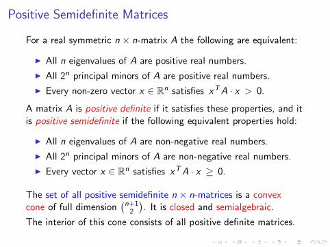
Positive Semidefinite Matrices
For a real symmetric n × n-matrix A the following are equivalent:
◮ All n eigenvalues of A are positive real numbers.
◮ All 2n principal minors of A are positive real numbers.
◮ Every non-zero vector x ∈ Rn satisfies xTA · x > 0.
A matrix A is positive definite if it satisfies these properties, and itis positive semidefinite if the following equivalent properties hold:
◮ All n eigenvalues of A are non-negative real numbers.
◮ All 2n principal minors of A are non-negative real numbers.
◮ Every vector x ∈ Rn satisfies xT A · x ≥ 0.
The set of all positive semidefinite n × n-matrices is a convexcone of full dimension
(
n+1
2
)
. It is closed and semialgebraic.
The interior of this cone consists of all positive definite matrices.

Semidefinite Programming
A spectrahedron is the intersection of the cone of positivesemidefinite matrices with an affine-linear space. Its algebraicrepresentation is a linear combination of symmetric matrices
A0 + x1A1 + x2A2 + · · · + xmAm � 0 (∗)
Engineers call this is a linear matrix inequality.

Semidefinite Programming
A spectrahedron is the intersection of the cone of positivesemidefinite matrices with an affine-linear space. Its algebraicrepresentation is a linear combination of symmetric matrices
A0 + x1A1 + x2A2 + · · · + xmAm � 0 (∗)
Engineers call this is a linear matrix inequality.
Semidefinite programming is the computational problemof maximizing a linear function over a spectrahedron:
Maximize c1x1 + c2x2 + · · · + cmxm subject to (∗)
Example: The smallest eigenvalue of a symmetric matrix A is
the solution of the SDP Maximize x subject to A − x · Id � 0.
Convex PolyhedraLinear programming is semidefinite programming for diagonalmatrices. If A0,A1, . . . ,Am are diagonal n×n-matrices then
A0 + x1A1 + x2A2 + · · · + xmAm � 0
translates into a system of n linear inequalities in the m unknowns.
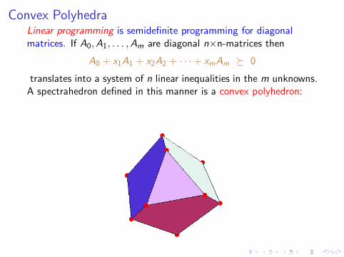
Convex PolyhedraLinear programming is semidefinite programming for diagonalmatrices. If A0,A1, . . . ,Am are diagonal n×n-matrices then
A0 + x1A1 + x2A2 + · · · + xmAm � 0
translates into a system of n linear inequalities in the m unknowns.A spectrahedron defined in this manner is a convex polyhedron:

Pictures in Dimension TwoHere is a picture of a spectrahedron for m = 2 and n = 3:

Pictures in Dimension TwoHere is a picture of a spectrahedron for m = 2 and n = 3:
Duality is important in convex optimization:

Example: Multifocal Ellipses
Given m points (u1, v1), . . . , (um, vm) in the plane R2, and
a radius d > 0, their m-ellipse is the convex algebraic curve
{
(x , y) ∈ R2 :
m∑
k=1
√
(x−uk)2 + (y−vk)2 = d
}
.
The 1-ellipse and the 2-ellipse are algebraic curves of degree 2.

Example: Multifocal Ellipses
Given m points (u1, v1), . . . , (um, vm) in the plane R2, and
a radius d > 0, their m-ellipse is the convex algebraic curve
{
(x , y) ∈ R2 :
m∑
k=1
√
(x−uk)2 + (y−vk)2 = d
}
.
The 1-ellipse and the 2-ellipse are algebraic curves of degree 2.
The 3-ellipse is an algebraic curve of degree 8:

2, 2, 8, 10, 32, ...The 4-ellipse is an algebraic curve of degree 10:
The 5-ellipse is an algebraic curve of degree 32:

Concentric Ellipses
What is the algebraic degree of the m-ellipse?How to write its equation?
What is the smallest radius d for which the m-ellipse isnon-empty? How to compute the Fermat-Weber point?

3D View
C =
{
(x , y , d) ∈ R3 :
m∑
k=1
√
(x−uk)2 + (y−vk)2 ≤ d
}
.

Ellipses are SpectrahedraThe 3-ellipse with foci (0, 0), (1, 0), (0, 1) has the representation
2
6
6
6
6
6
6
6
6
6
4
d + 3x − 1 y − 1 y 0 y 0 0 0
y − 1 d + x − 1 0 y 0 y 0 0
y 0 d + x + 1 y − 1 0 0 y 0
0 y y − 1 d − x + 1 0 0 0 y
y 0 0 0 d + x − 1 y − 1 y 0
0 y 0 0 y − 1 d − x − 1 0 y
0 0 y 0 y 0 d − x + 1 y − 1
0 0 0 y 0 y y − 1 d − 3x + 1
3
7
7
7
7
7
7
7
7
7
5
The ellipse consists of all points (x , y) where this symmetric8×8-matrix is positive semidefinite. Its boundary is a curveof degree eight:
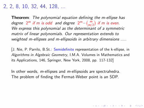
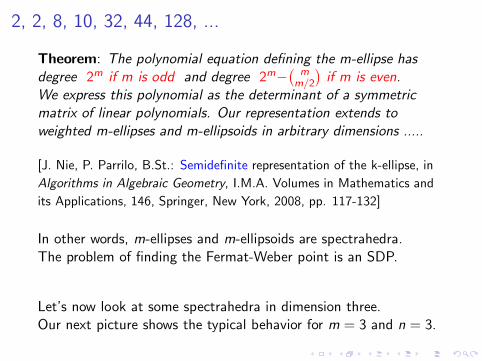
2, 2, 8, 10, 32, 44, 128, ...
Theorem: The polynomial equation defining the m-ellipse has
degree 2m if m is odd and degree 2m−(
mm/2
)
if m is even.
We express this polynomial as the determinant of a symmetric
matrix of linear polynomials. Our representation extends to
weighted m-ellipses and m-ellipsoids in arbitrary dimensions .....
[J. Nie, P. Parrilo, B.St.: Semidefinite representation of the k-ellipse, in
Algorithms in Algebraic Geometry, I.M.A. Volumes in Mathematics and
its Applications, 146, Springer, New York, 2008, pp. 117-132]
In other words, m-ellipses and m-ellipsoids are spectrahedra.The problem of finding the Fermat-Weber point is an SDP.
Let’s now look at some spectrahedra in dimension three.Our next picture shows the typical behavior for m = 3 and n = 3.
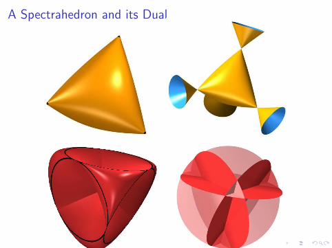
A Spectrahedron and its Dual

Non-Linear Convex Hull Computation
Input :{
(t, t2, t3) ∈ R3 : −1 ≤ t ≤ 1
}
−1
−0.5
0
0.5
1
0
0.5
1−1
−0.8
−0.6
−0.4
−0.2
0
0.2
0.4
0.6
0.8
1
y1y
2
y 3
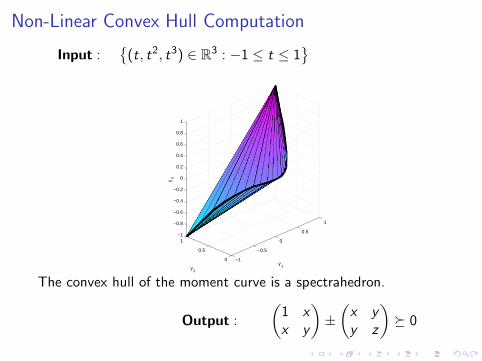
Non-Linear Convex Hull Computation
Input :{
(t, t2, t3) ∈ R3 : −1 ≤ t ≤ 1
}
−1
−0.5
0
0.5
1
0
0.5
1−1
−0.8
−0.6
−0.4
−0.2
0
0.2
0.4
0.6
0.8
1
y1y
2
y 3
The convex hull of the moment curve is a spectrahedron.
Output :
(
1 x
x y
)
±(
x y
y z
)
� 0
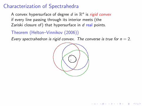
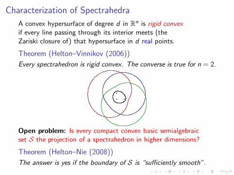
Characterization of Spectrahedra
A convex hypersurface of degree d in Rn is rigid convex
if every line passing through its interior meets (theZariski closure of) that hypersurface in d real points.
Theorem (Helton–Vinnikov (2006))
Every spectrahedron is rigid convex. The converse is true for n = 2.
Characterization of Spectrahedra
A convex hypersurface of degree d in Rn is rigid convex
if every line passing through its interior meets (theZariski closure of) that hypersurface in d real points.
Theorem (Helton–Vinnikov (2006))
Every spectrahedron is rigid convex. The converse is true for n = 2.
Open problem: Is every compact convex basic semialgebraicset S the projection of a spectrahedron in higher dimensions?
Theorem (Helton–Nie (2008))
The answer is yes if the boundary of S is “sufficiently smooth”.

Questions about 3-Dimensional Spectrahedra
What are the edge graphs of spectrahedra in R3?
How can one define their combinatorial types?
Is there an analogue to Steinitz’ Theorem for polytopes in R3?
Consider 3-dimensional spectrahedra whose boundary is anirreducible surface of degree n. Can such a spectrahedron have(
n+1
3
)
isolated singularities in its boundary? How about n = 4?
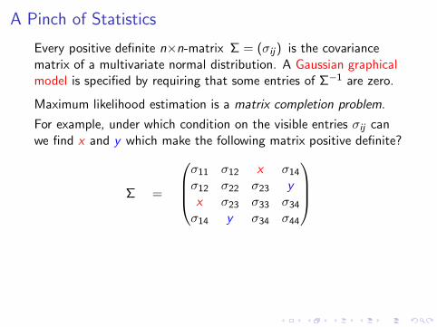
A Pinch of Statistics
Every positive definite n×n-matrix Σ = (σij) is the covariancematrix of a multivariate normal distribution. A Gaussian graphicalmodel is specified by requiring that some entries of Σ−1 are zero.
Maximum likelihood estimation is a matrix completion problem.
For example, under which condition on the visible entries σij canwe find x and y which make the following matrix positive definite?
Σ =
σ11 σ12 x σ14
σ12 σ22 σ23 y
x σ23 σ33 σ34
σ14 y σ34 σ44
The MLE is the point (x , y) which maximizes the determinant.In optimization, this is the analytic center of the spectrahedron.
[C. Uhler, B.St.: Multivariate Gaussians, Semidefinite
Matrix Completion and Convex Algebraic Geometry, 2009]

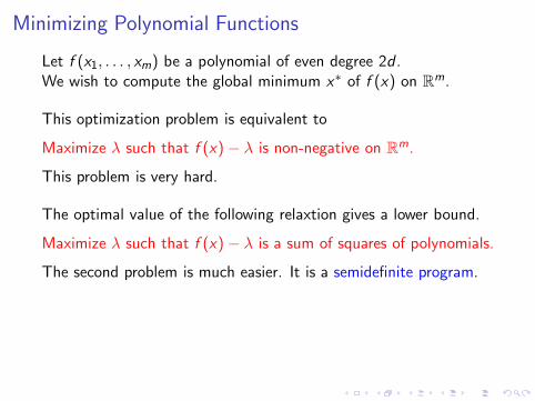
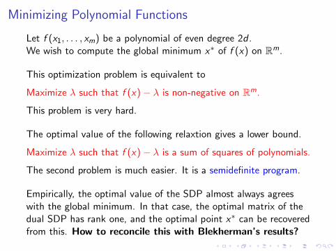
Minimizing Polynomial Functions
Let f (x1, . . . , xm) be a polynomial of even degree 2d .We wish to compute the global minimum x∗ of f (x) on R
m.
This optimization problem is equivalent to
Maximize λ such that f (x) − λ is non-negative on Rm.
This problem is very hard.
Minimizing Polynomial Functions
Let f (x1, . . . , xm) be a polynomial of even degree 2d .We wish to compute the global minimum x∗ of f (x) on R
m.
This optimization problem is equivalent to
Maximize λ such that f (x) − λ is non-negative on Rm.
This problem is very hard.
The optimal value of the following relaxtion gives a lower bound.
Maximize λ such that f (x) − λ is a sum of squares of polynomials.
The second problem is much easier. It is a semidefinite program.
Empirically, the optimal value of the SDP almost always agreeswith the global minimum. In that case, the optimal matrix of thedual SDP has rank one, and the optimal point x∗ can be recoveredfrom this. How to reconcile this with Blekherman’s results?

SOS Programming: A Univariate Example
Let m = 1, d = 2 and f (x) = 3x4 + 4x3 − 12x2. Then
f (x) − λ =(
x2 x 1)
3 2 µ − 62 −2µ 0
µ − 6 0 −λ
x2
x
1
Our problem is to find (λ, µ) such that the 3×3-matrix is positivesemidefinite and λ is maximal. The optimal solution of this SDP is
(λ∗, µ∗) = (−32,−2).
Cholesky factorization reveals the SOS representation
f (x) − λ∗ =(
(√
3 x − 4√3) · (x + 2)
)2+
8
3
(
x + 2)2
.
We see that the global minimum is x∗ = −2.This approach works for many polynomial optimization problems.

Hankel Matrices
Consider the intersection of the cone of 6×6 PSD matrices withthe 15-dimensional linear space consisting of all Hankel matrices
H =
λ400 λ220 λ202 λ310 λ301 λ211
λ220 λ040 λ022 λ130 λ121 λ031
λ202 λ022 λ004 λ112 λ103 λ013
λ310 λ130 λ112 λ220 λ211 λ121
λ301 λ121 λ103 λ211 λ202 λ112
λ211 λ031 λ013 λ121 λ112 λ022
.
Dual to this intersection is the projection
Sym2(Sym2(R3)) → Sym4(R
3)
taking a 6×6-matrix to the ternary quartic it represents. Its imageis a cone whose algebraic boundary is a discriminant of degree 27.
Problem: Determine the variety of all Bezout matrices H−1.

Orbitopes
An orbitope is the convex hull of an orbit under a real algebraicrepresentation of a compact Lie group. Primary examples arethe groups SO(n) and their products. Orbitopes for their adjointrepresentations are continuous analogues of permutohedra.
Many of these special orbitopes are projections of spectrahedra.
A forthcoming paper with Raman Sanyal and Frank Sottiledevelops the basic theory of orbitopes and has many examples.
Example: Consider the orbitope of (x+y+z)4 under theSO(3)-action on the space Sym4(R
3) of ternary quartics.
Quiz: Is this orbitope a spectrahedron?
Answer: Yes, it is the set of psd Hankel matrices H that satisfy
λ400 + λ040 + λ004 + 2λ220 + 2λ202 + 2λ022 = 9.
Problem. Classify all SO(n)-orbitopes that are spectrahedra.
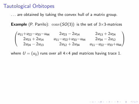
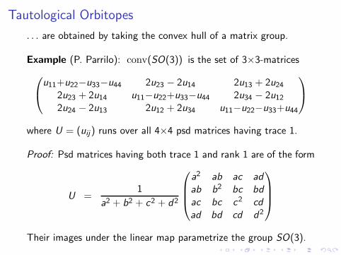
Tautological Orbitopes
. . . are obtained by taking the convex hull of a matrix group.
Example (P. Parrilo): conv(SO(3)) is the set of 3×3-matrices
u11+u22−u33−u44 2u23 − 2u14 2u13 + 2u24
2u23 + 2u14 u11−u22+u33−u44 2u34 − 2u12
2u24 − 2u13 2u12 + 2u34 u11−u22−u33+u44
where U = (uij) runs over all 4×4 psd matrices having trace 1.
Proof: Psd matrices having both trace 1 and rank 1 are of the form
U =1
a2 + b2 + c2 + d2
a2 ab ac ad
ab b2 bc bd
ac bc c2 cd
ad bd cd d2
Their images under the linear map parametrize the group SO(3).

Barvinok-Novik OrbitopesConsider the SO(2)×SO(2)-orbitope BN4 determined by the curve
θ 7→(
cos(θ), sin(θ), cos(3θ), sin(3θ))
∈ R4.
This is the projection of a 6-dimensional Hermitian spectrahedron:
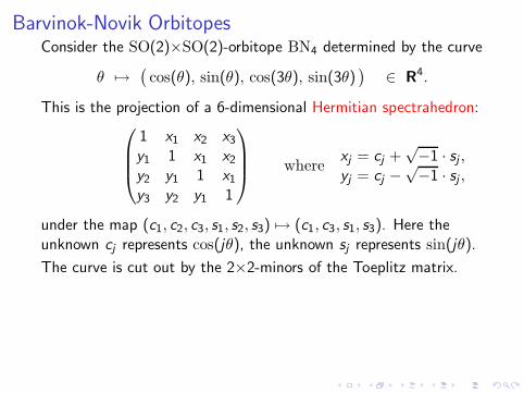
Barvinok-Novik OrbitopesConsider the SO(2)×SO(2)-orbitope BN4 determined by the curve
θ 7→(
cos(θ), sin(θ), cos(3θ), sin(3θ))
∈ R4.
This is the projection of a 6-dimensional Hermitian spectrahedron:
1 x1 x2 x3
y1 1 x1 x2
y2 y1 1 x1
y3 y2 y1 1
wherexj = cj +
√−1 · sj ,
yj = cj −√−1 · sj ,
under the map (c1, c2, c3, s1, s2, s3) 7→ (c1, c3, s1, s3). Here theunknown cj represents cos(jθ), the unknown sj represents sin(jθ).
The curve is cut out by the 2×2-minors of the Toeplitz matrix.
The faces of BN4 are certain edges and triangles. Its algebraicboundary is the threefold defined by the degree 8 polynomial
x23 y6
1 − 2x31 x3y
31 y3 + x6
1 y23 + 4x3
1 y31 − 6x1x3y
41 − 6x4
1 y1y3 + 12x21 x3y
21 y3
− 2x23 y3
1 y3 − 2x31 x3y
23 − 3x2
1 y21 + 4x3y
31 + 4x3
1 y3 − 6x1x3y1y3 + x23y2
3 .

Conclusion
Spectrahedra and orbitopes deserve to be studied in their ownright, independently of their important uses in applications.
A true understanding of these convex bodies will requirethe integration of three different areas of mathematics:
◮ Classical Convexity
◮ Algebraic Geometry
◮ Optimization Theory


