1

Semidefinite Programming Approach to GaussianSequential Rate-Distortion Trade-offs

Takashi Tanaka, Kwang-Ki K. Kim, Pablo A. Parrilo, and Sanjoy K. Mitter

Abstract—Sequential rate-distortion (SRD) theory provides aframework for studying the fundamental trade-off between data-rate and data-quality in real-time communication systems. In thispaper, we consider the SRD problem for multi-dimensional time-varying Gauss-Markov processes under mean-square distortioncriteria. We first revisit the sensor-estimator separation principle,which asserts that considered SRD problem is equivalent to ajoint sensor and estimator design problem in which data-rate ofthe sensor output is minimized while the estimator’s performancesatisfies the distortion criteria. We then show that the optimaljoint design can be performed by semidefinite programming. Asemidefinite representation of the corresponding SRD functionis obtained. Implications of the obtained result in the context ofzero-delay source coding theory and applications to networkedcontrol theory are also discussed.

Index Terms—Control over communications; LMIs; Optimiza-tion algorithms; Stochastic optimal control; Kalman filtering

I. INTRODUCTION

In this paper, we study a fundamental performance limita-tion of zero-delay communication systems using the sequentialrate-distortion (SRD) theory. Suppose that xt is an Rn-valueddiscrete time random process with known statistical properties.At every time step, the encoder observes a realization of thesource xt and generates a binary sequence bt ∈ 0, 1lt oflength lt, which is transmitted to the decoder. The decoderproduces an estimation zt of xt based on the messages bt

received up to time t. Both encoder and decoder have infinitememories of the past. A zero-delay communication system isdetermined by a selected encoder-decoder pair, whose perfor-mance is analyzed in the trade-off between the rate (viz. theaverage number of bits that must be transmitted per time step)and the distortion (viz. the discrepancy between the sourcesignal xt and the reproduced signal zt). The region in the rate-distortion plane achievable by a zero-delay communicationsystem is referred to as the zero-delay rate-distortion region.1

The standard rate-distortion region identified by Shannononly provides a conservative outer bound of the zero-delayrate-distortion region. This is because, in general, achievingthe standard rate-distortion region requires the use of antic-ipative (non-causal) codes (e.g., [1, Theorem 10.2.1]). It iswell known that the standard rate-distortion region can be

T. Tanaka is with ACCESS Linnaeus Center, KTH Royal Institute ofTechnology, Stockholm, 10044 Sweden.

P. A. Parrilo, and S. K. Mitter are with the Laboratory for Information andDecision Systems, Massachusetts Institute of Technology, Cambridge, MA,02139 USA.

K.-K. K. Kim is with the Electronic Control Development Team of HyundaiMotor Company (HMC) Research & Development Division in South Korea.

1Formal definition of the zero-delay rate-distortion region is given inSection VI-A.

expressed by the rate-distortion function2 for general sources.In contrast, description of the zero-delay rate-distortion regionrequires more case-dependent knowledge of the optimal sourcecoding schemes. For scalar memoryless sources, it is shownthat the optimal performance of zero-delay codes is achievableby a scalar quantizer [2]. Witsenhausen [3] showed that forthe k-th order Markov sources, there exists an optimal zero-delay quantizer with memory structure of order k. Neuhoffand Gilbert considered entropy-coded quantizers within theclass of causal source codes [4], and showed that for memo-ryless sources, the optimal performance is achievable by time-sharing memoryless codes. This result is extended to sourceswith memory in [5]. An optimal memory structure of zero-delay quantizers for partially observable Markov processes onabstract (Polish) spaces is identified in [6]. The rate of finite-delay source codes for general sources and general distortionmeasures is analyzed in [7]. Zero-delay or finite-delay jointsource-channel coding problems have also been studied in theliterature; [8]–[11] to name a few.

In [12], [13], Tatikonda et al. studied the zero-delay rate-distortion region using a quantity called sequential rate-distortion function,3 which is defined as the infimum of theMassey’s directed information [18] from the source process tothe reproduction process subject to the distortion constraint.Although the SRD function does not coincide with the bound-ary of the zero-delay rate-distortion region in general, it isrecently shown that the SRD function provides a tight outerbound of the zero-delay rate-distortion region achievable byuniquely decodable codes [16], [19]. This observation showsan intimate connection between the SRD function and the fun-damental performance limitations of real-time communicationsystems. For this reason, we consider the SRD function as themain object of interest in this paper.

Closely related quantity to the SRD function was studiedby Gorbunov and Pinsker [14] in the early 1970’s. Bucy [15]derived the SRD function for Gauss-Markov processes in asimple case. In his approach, the problem of deriving theSRD function for Gauss-Markov processes under mean-squaredistortion criteria (which henceforth will be simply referred toas the Gaussian SRD problem) is viewed as a sensor-estimatorjoint design problem to minimize the estimation error subject

2This quantity is defined by the infimum of the mutual information betweenthe source and the reproduction subject to the distortion constraint [1, Theorem10.2.1].

3Closely related or apparently equivalent notions to the sequential rate-distortion function have been given various names in the literature, in-cluding nonanticipatory ε-entropy [14], constrained distortion rate function[15], causal rate-distortion function [16], and nonanticipative rate-distortionfunction [17].

arX

iv:1

411.

7632

v3 [

mat

h.O

C]

9 A

ug 2

016

2

to the data-rate constraint. This approach is justified by the“sensor-estimator separation principle,” which asserts that anoptimal solution (i.e., the optimal stochastic kernel, to bemade precise in the sequel) to the Gaussian SRD problem isrealizable by a two-stage mechanism with a linear-Gaussianmemoryless sensor and the Kalman filter. Although this fact isimplicitly shown in [12], [13], for completeness, we reproducea proof in this paper based on a technique used in [12], [13].

The sensor-estimator separation principle gives us a struc-tural understanding of the Gaussian SRD problem. In partic-ular, based on this principle, we show that the Gaussian SRDproblem can be formulated as a semidefinite programmingproblem (Theorem 1), which is the main contribution of thispaper. We derive a computationally accessible form (namelya semidefinite representation4 [20]) of the SRD function, andprovide an efficient algorithm to solve Gaussian SRD problemsnumerically.

The semidefinite representation of the SRD function may becompared with an alternative analytical approach via Duncan’stheorem, which states that “twice the mutual information ismerely the integration of the trace of the optimal mean squarefiltering error” [21]. Duncan’s result was significantly gener-alized as the “I-MMSE” relationships in non-causal [22] andcausal [23] estimation problems. Our SDP-based approachesare applicable to the cases with multi-dimensional and time-varying Gauss-Markov sources to which the existing I-MMSEformulas cannot be applied straightforwardly. Although wefocus on the Gaussian SRD problems in this paper, wenote that the standard RD and SRD problems for generalsources and distortion measures in abstract (Polish) spaces arediscussed in [24] and [17], respectively.

This paper is organized as follows. In Section II, weformally introduce the Gaussian SRD problem, which is themain problem considered in this paper. In Section III, weshow that the Gaussian SRD problem is equivalent to whatwe call the linear-Gaussian sensor design problem, whichformally establishes the sensor-estimator separation principle.Then, in Section IV, we show that the linear-Gaussian sensordesign problem can be reduced to an SDP problem, whichthus provides us an SDP-based solution synthesis procedurefor Gaussian SRD problems. Extensions to stationary andinfinite horizon problems are given in Section V. In Sec-tion VI, we consider applications of SRD theory to real-time communication systems and networked control systems.Simple simulation results will be presented in Section VII. Weconclude in Section VIII.

Notation: Let X be an Euclidean space, and BX be theBorel σ-algebra on X . Let (Ω,F ,P) be a probability space,and x : (Ω,F)→ (X ,BX ) be a random variable. Throughoutthe paper, we use lower case boldface symbols such as x todenote random variables, while x ∈ X is a realization of x.We denote by qx the probability measure of x defined byqx(A) = P(ω : x(ω) ∈ A) for every A ∈ BX . Whenno confusion occurs, this measure will be also denoted byqx(x) or q(x). For a Borel measurable function f : X → R,

4To be precise, we show that the exponentiated SRD function for multidi-mensional Gauss-Markov source is semidefinite representable by (27).

we write Ef(x) ,∫f(x)qx(dx). For a random vector, we

write xt , (x0, · · · ,xt) or xt , (x1, · · · ,xt) depending onthe initial index, and xts , (xs, · · · ,xt). Let Θ be a realsymmetric matrix of size n×n. Notations Θ 0 or Θ ∈ Sn++

(resp. Θ 0 or Θ ∈ Sn+) mean that Θ is a positive definite(resp. positive semidefinite) matrix. For a positive semidefinitematrix Θ, we write ‖x‖Θ ,

√x>Θx.

II. PROBLEM FORMULATION

We begin our discussion with an estimation-theoretic inter-pretation of a simple rate-distortion trade-off problem. Recallthat a rate-distortion problem for a scalar Gaussian randomvariable x ∼ N (0, 1) with the mean square distortion con-straint is an optimization problem of the following form:

min I(x; z) (1)

s.t. E(x− z)2 ≤ D.

Here, z is a reproduction of the source x, and I(x; z) denotesthe mutual information between x and z. The minimizationis over the space of reproduction policies, i.e., stochastickernels q(dz|x). The optimal value of (1) is known as therate-distortion function, R(D), and can be explicitly obtained[1] as

R(D) = max

0,

1

2log

(1

D

).

It is also possible to write the optimal reproduction policyq(dz|x) explicitly. To this end, consider a linear sensor

y = cx + v (2)

where v ∼ N (0, σ2) is a Gaussian noise independent of x.Also, let

z = E(x|y) (3)

be the least mean square error estimator of x given y. Noticethat the right hand side of (3) is given by c

c2+σ2y. Then, itcan be shown that an optimal solution q(dz|x) to (1) is acomposition of (2) and (3), provided that the signal-to-noiseratio of the sensor (2) is chosen to be

SNR ,c2

σ2= max

0,

1

D− 1

. (4)

This gives us the following notable observations:• Fact 1: A “sensor-estimator separation principle” holds for

the Gaussian rate-distortion problem (1), in the sense thatan optimal reproduction policy q(dz|x) can be written as atwo-stage mechanism with a linear sensor mechanism (2)and a least mean square error estimator (3).

• Fact 2: The original infinite dimensional optimizationproblem (1) with respect to q(dz|x) is reduced to a simpleoptimization problem in terms of a scalar parameter SNR.Moreover, for a given D > 0, the optimal choice of SNRis given by a closed-form expression (4).

These facts can be significantly generalized, and serve as aguideline to develop a solution synthesis for Gaussian SRDproblems in this paper.

3

A. Gaussian SRD problem

The Gaussian SRD problem can be viewed as a generaliza-tion of (1). Let xt be an Rnt -valued Gauss-Markov process

xt+1 = Atxt + wt, t = 0, 1, · · · , T − 1 (5)

where x0 ∼ N (0, P0), P0 0 and wt ∼ N (0,Wt),Wt 0for t = 0, 1, · · · , T − 1 are mutually independet Gaussianrandom variables. The Gaussian SRD problem is formulatedas

(P-SRD): minγ∈Γ

I(xT → zT ) (6a)

s.t. E‖xt − zt‖2Θt≤ Dt (6b)

where (6b) is imposed for every t = 1, · · · , T . Here, zt isan Rnt -valued reproduction of xt. The minimization (6a)is over the space Γ of zero-delay reproduction policies of ztgiven xt and zt−1, i.e., the sequences of causal stochastickernels5 γ = ⊗Tt=1q(dzt|xt, zt−1). The term I(xT → zT )is known as directed information, introduced by Massey [18]following Marko’s earlier work [25], and is defined by

I(xT → zT ) ,T∑t=1

I(xt; zt|zt−1). (7)

The Gaussian SRD problem is visualized in Fig. 1.Remark 1: Directed information measures the amount of

information flow from xt to zt and is not symmetric, i.e.,I(xT → zT ) 6= I(zT → xT ) in general. However, when theprocess zt is causally dependent on xt and xt is notaffected by zt, it can be shown [26] that I(xT → zT ) =I(xT ; zT ). By definition of our source process (5), there is noinformation feedback from zt to xt, and thus I(xT →zT ) = I(xT ; zT ) holds in our setup. Hence, I(xT ; zT ) canbe equivalently used as an objective in (P-SRD). However, wechoose to use I(xT → zT ) for the future considerations (e.g.,[27]) in which xt is a controlled stochastic process and isdependent on zt. In such cases, I(xT ; zT ) and I(xT → zT )are not equal, and the latter is a more meaningful quantity inmany applications.

Since (P-SRD) is an infinite dimensional optimization prob-lem, it is difficult to apply numerical methods directly. Hence,we first need to develop a structural understanding of itssolution. It turns out that the sensor-estimator separationprinciple still holds for (P-SRD), and this observation playsan important role in the subsequent sections. We are goingto establish the following facts:• Fact 1’: A sensor-estimator separation principle holds for

the Gaussian SRD problem. That is, an optimal policy⊗Tt=1q(dzt|xt, zt−1) for (P-SRD) can be realized as acomposition of a sensor mechanism

yt = Ctxt + vt, t = 1, 2, · · · , T (8)

where vt ∼ N (0, Vt), Vt 0 are mutually independentGaussian random variables, and the least mean square errorestimator (Kalman filter)

zt = E(xt|yt), t = 1, 2, · · · , T. (9)

5See Appendix A for a formal description of causal stochastic kernels.

Gauss-Markov Process

Linear-Gaussian Sensor

(To be designed) 𝑦𝑡 = 𝐶𝑡𝑥𝑡+𝑣𝑡

Kalman Filter 𝑧𝑡 = 𝔼 𝑥𝑡|𝑦

𝑡

𝑧𝑡 𝑦𝑡 𝑥𝑡

min 𝐼 𝑥𝑡; 𝑦𝑡|𝑦𝑡−1𝑇

𝑡=1 s.t. 𝔼 𝑥𝑡 − 𝑧𝑡2 ≤ 𝐷𝑡

Gauss-Markov Process

Causal Stochastic Kernel (To be designed) 𝑞 𝑑𝑧𝑡|𝑥

𝑡, 𝑧𝑡−1

𝑧𝑡 𝑥𝑡

min 𝐼 𝑥𝑡; 𝑧𝑡|𝑧𝑡−1𝑇

𝑡=1 s.t. 𝔼 𝑥𝑡 − 𝑧𝑡2 ≤ 𝐷𝑡

Fig. 1. The Gaussian sequential rate-distortion problem (P-SRD).

Gauss-Markov Process

Linear-Gaussian Sensor

(To be designed) 𝑦𝑡 = 𝐶𝑡𝑥𝑡+𝑣𝑡

Kalman Filter 𝑧𝑡 = 𝔼 𝑥𝑡|𝑦

𝑡

𝑧𝑡 𝑦𝑡 𝑥𝑡

min 𝐼 𝑥𝑡; 𝑦𝑡|𝑦𝑡−1𝑇

𝑡=1 s.t. 𝔼 𝑥𝑡 − 𝑧𝑡2 ≤ 𝐷𝑡

Gauss-Markov Process

Causal Stochastic Kernel (To be designed) 𝑞 𝑧𝑡|𝑥

𝑡, 𝑧𝑡−1

𝑧𝑡 𝑥𝑡

min 𝐼 𝑥𝑡; 𝑧𝑡|𝑧𝑡−1𝑇

𝑡=1 s.t. 𝔼 𝑥𝑡 − 𝑧𝑡2 ≤ 𝐷𝑡

Fig. 2. The linear-Gaussian sensor design problem (P-LGS).

• Fact 2’: The original optimization problem (P-SRD) overan infinite-dimensional space Γ is reduced to an optimiza-tion problem over a finite-dimensional space of matrix-valued signal-to-noise ratios of the sensor (8), defined by

SNRt , C>t V−1t Ct 0, t = 1, 2, · · · , T. (10)

Moreover, the optimal SNRtTt=1, which depends on Dt >0, t = 1, · · · , T , can be obtained by SDP.

Unlike (4), an analytical expression of the optimal SNRtTt=1

may not be available. Nevertheless, we will show that they canbe easily obtained by SDP.

B. Linear-Gaussian sensor design problem

In Section III, we establish the sensor-estimator separationprinciple. To this end, we show that (P-SRD) is equivalent towhat we call the linear-Gaussian sensor design problem (P-LGS) visualized in Fig. 2. Formally, (P-LGS) is formulated as

(P-LGS): minγ∈ΓLGS

T∑t=1

I(xt;yt|yt−1) (11a)

s.t. E‖xt − zt‖2Θt≤ Dt (11b)

where (11b) is imposed for every t = 1, · · · , T . We assumethat yt is produced by a linear-Gaussian sensor (8), andzt is produced by the Kalman filter (9). In other words,the optimization domain ΓLGS ⊂ Γ is the space of causalstochastic kernels with a separation structure (8) and (9),which is parameterized by a sequence of matrices Ct, VtTt=1.Intuitively, I(xt;yt|yt−1) in (11a) can be understood as theamount of information acquired by the sensor (8) at time t. Wecall this problem a “sensor design problem” because our focusis on choosing an optimal sensing gain Ct in (8) and the noisecovariance Vt. Notice that perfect observation with Ct = I andVt = 0 is trivially the best to minimize the estimation errorin (11b) (in fact, E‖xt− zt‖2Θt

= 0 is achieved), but it incurssignificant information cost (i.e., I(xt;yt|yt−1) = +∞), andhence it is not an optimal solution to (P-LGS).

4

Remark 2: In (P-LGS), we search for the optimal Ct ∈Rrt×n and Vt ∈ Srt++. However, the sensor dimension rt isnot given a priori, and choosing it optimally is part of theproblem. In particular, if making no observation is the optimalsensing at some specific time instance t, we should be able torecover rt = 0 as an optimal solution.

Although the objective functions (6a) and (11a) appeardifferently, it will be shown in Section III that they coincidein the domain ΓLGS. Moreover, in the same section it willbe shown that an optimal solution to (P-SRD) can alwaysbe found in the domain ΓLGS. These observations imply thatone can obtain an optimal solution to (P-SRD) by solving (P-LGS).

C. Stationary casesWe will also consider a time-invariant system

xt+1 = Axt + wt, t = 0, 1, 2, · · · (12)

where xt is an Rn-valued random variable with x0 ∼N (0, P0), and wt ∼ N (0,W ) is a stationary white Gaussiannoise. We assume P0 0 and W 0. Stationary and infinitehorizon version of the Gaussian SRD problem is formulatedas

min lim supT→∞

1

TI(xT → zT ) (13a)

s.t. lim supT→∞

1

T

T∑t=1

E‖xt − zt‖2Θ ≤ D. (13b)

This is an optimization over the sequence of stochastic kernels⊗t∈N q(dzt|xt, zt−1). The optimal value of (13) as a functionof the average distortion D is referred to as the sequentialrate-distortion function, and is denoted by RSRD(D).

Similarly, a stationary and infinite horizon version of thelinear-Gaussian sensor design problem is formulated as

min lim supT→∞

1

T

T∑t=1

I(xt;yt|yt−1) (14a)

s.t. lim supt→∞

1

T

T∑t=1

E‖xt − zt‖2Θ ≤ D. (14b)

Here, we assume yt = Ctxt+vt where vt ∼ N (0, Vt), Vt 0is a mutually independent Gaussian stochastic process andzt = E(xt|yt). Design variables in (14) are Ct, Vtt∈N.Again, determining their dimensions is part of the problem.

D. Soft- vs. hard-constrained problemsIntroducing Lagrange multipliers αt > 0, one can also

consider a soft-constrained version of (P-SRD):

min I(xT → zT ) +αt2E‖xt − zt‖2Θt

(15)

Similarly to the Lagrange multiplier theorem (e.g., Proposition3.1.1 in [28]), it is possible to show that there exists a setof multipliers such that an optimal solution to (15) is alsoan optimal solution to (P-SRD). We will prove this fact inSection IV after we establish that both (P-SRD) and (15)can be transformed as finite dimensional convex optimizationproblems. For this reason, we refer to both (P-SRD) and (15)as Gaussian SRD problems.

III. SENSOR-ESTIMATOR SEPARATION PRINCIPLE

Let f∗SRD and f∗LGS be the optimal values of (P-SRD) and(P-LGS) respectively. In this section, we show that f∗SRD =f∗LGS, and an optimal solution γ ∈ ΓLGS to (P-LGS) is also anoptimal solution to (P-SRD). This result establishes the sensor-estimator separation principle (Fact 1’). We introduce anotheroptimization problem (P-1), which serves as an intermediatestep to establish this fact.

(P-1): minγ∈Γ1

T∑t=1

I(xt; zt|zt−1)

s.t. E‖xt − zt‖2Θt≤ Dt.

The optimization is over the space Γ1 of linear-Gaussianstochastic kernels γ = ⊗Tt=1 q(dzt|xt, zt−1), where eachstochastic kernel q(dzt|xt, zt−1) is of the form

zt = Etxt + Ft,t−1zt−1 + · · ·+ Ft,1z1 + gt (16)

where Et, Ft,t−1, · · · , Ft,1 are some matrices with appropri-ate dimensions, and gt is a zero-mean, possibly degenerateGaussian random variable that is independent of x0,w

t,gt−1.Notice that ΓLGS ⊂ Γ1 ⊂ Γ. The underlying Gauss-Markovprocess xt is defined by (5). Let f∗1 be the optimal valueof (P-1). The next lemma claims the equivalence between (P-SRD) and (P-1).

Lemma 1:(i) If there exists γ ∈ Γ attaining a value fSRD < +∞ of the

objective function in (P-SRD), then there exists γ1 ∈ Γ1

attaining a value f1 ≤ fSRD of the objective function in(P-1).

(ii) Every γ1 ∈ Γ1(⊂ Γ) attaining f1 < +∞ in (P-1) alsoattains fSRD = f1 in (P-SRD).

Lemma 1 is the most significant result in this section, whichessentially guarantees the linearity of an optimal solution to theGaussian SRD problems. The proof of Lemma 1 can be foundin Appendix B. The basic idea of proof relies on the well-known fact that Gaussian distribution maximizes entropy whencovariance is fixed. This proposition appears as Lemma 4.3 in[13], but we modified the proof using the Radon-Nikodymderivatives so that the proof does not require the existence ofprobability density functions. The next lemma establishes theequivalence between (P-1) and (P-LGS).

Lemma 2:(i) If there exists γ1 ∈ Γ1 attaining a value f1 < +∞ of the

objective function in (P-1), then there exists γLGS ∈ ΓLGSattaining a value fLGS ≤ f1 of the objective function in(P-LGS).

(ii) Every γLGS ∈ ΓLGS(⊂ Γ1) attaining fLGS < +∞ in(P-LGS) also attains f1 ≤ fLGS in (P-1).

Proof of Lemma 2 is in Appendix C. Combining the abovetwo lemmas, we obtain the following consequence, which isthe main proposition in this section. It guarantees that we canalternatively solve (P-LGS) in order to solve (P-SRD).

Proposition 1: Suppose f∗SRD < +∞. Then there exists anoptimal solution γLGS ∈ ΓLGS(⊂ Γ) to (P-LGS). Moreover,an optimal solution to (P-LGS) is also an optimal solution to(P-SRD), and f∗SRD = f∗LGS.

5

IV. SDP-BASED SYNTHESIS

In this section, we develop an efficient numerical algorithmto solve (P-LGS). Due to the preceding discussion, this isequivalent to developing an algorithm to solve (P-SRD). Let(5) be given. Assume temporarily that (8) is also fixed. TheKalman filtering formula for computing zt = E(xt|yt) is

zt = zt|t−1+Pt|t−1C>t (CtPt|t−1C

>t +Vt)

−1(yt−Ctzt|t−1)

zt|t−1 = At−1zt−1

where Pt|t−1 is the covariance matrix of xt − E(xt|yt−1),which can be recursively computed as

Pt|t−1 = At−1Pt−1|t−1A>t−1 +Wt−1 (17a)

Pt|t = (P−1t|t−1 + SNRt)

−1 (17b)

for t = 1, · · · , T with P0|0 = P0. The variable SNRt is definedby (10). Using these quantities, mutual information terms in(11a) can be explicitly written as

I(xt;yt|yt−1)

= h(xt|yt−1)− h(xt|yt)

=1

2log det(At−1Pt−1|t−1A

>t−1+Wt−1)− 1

2log detPt|t.

Note that Wt 0 and Vt 0 guarantee that both differentialentropy terms are finite. Hence, (P-LGS) is equivalent tothe following optimization problem in terms of the variablesSNRt, Pt|tTt=1:

min

T∑t=1

1

2log det(At−1Pt−1|t−1A

>t−1 +Wt−1)

− 1

2log detPt|t (18a)

s.t. P−1t|t =(At−1Pt−1|t−1A

>t−1+Wt−1)−1+SNRt (18b)

SNRt 0,Tr(ΘtPt|t) ≤ Dt. (18c)

Equality (18b) is obtained by eliminating Pt|t−1 from (17).At this point, one may note that (18) can be viewed as anoptimal control problem with state Pt|t and control inputSNRt. Naturally, dynamic programming approach has beenproposed in the literature in similar contexts [10]–[12], [15].Alternatively, we next propose a method to transform (18)into an SDP problem. This allows us to solve (P-SRD) usingstandard SDP solvers, which is now a mature technology.

A. SRD optimization as max-det problem

Now we show that (18) can be converted to a determinantmaximization problem [29] subject to linear matrix inequalityconstraints. The first step is to transform (18) into an optimiza-tion problem in terms of Pt|tTt=1 only. This is possible bysimply replacing the nonlinear equality constraint (18b) witha linear inequality constraint

0 ≺ Pt|t At−1Pt−1|t−1A>t−1 +Wt−1.

This replacement eliminates SNRt from (18) giving us:

min

T∑t=1

1

2log det(At−1Pt−1|t−1A

>t−1 +Wt−1)

− 1

2log detPt|t (19a)

s.t. 0 ≺ Pt|t At−1Pt−1|t−1A>t−1 +Wt−1 (19b)

Tr(ΘtPt|t) ≤ Dt. (19c)

Note that (18) and (19) are mathematically equivalent, sinceeliminated SNR variables can be easily constructed fromPt|tTt=1 through

SNRt = P−1t|t − (At−1Pt−1|t−1A

>t−1 +Wt−1)−1. (20)

The second step is to rewrite the objective function (19a).Regrouping terms, (19a) can be written as a summation ofthe initial cost 1

2 log det(A0P0|0A>0 + W0), the final cost

− 12 log detPT |T , and stage-wise costs

1

2log det(AtPt|tA

>t +Wt)−

1

2log detPt|t (21)

for t = 1, · · · , T −1. Applying the matrix determinant lemma(e.g., Theorem 18.1.1 in [30]), (21) can be rewritten as

1

2log detWt −

1

2log det(P−1

t|t +A>t W−1t At)

−1. (22)

Due to the monotonicity of the determinant function, (22) isequal to the optimal value of

min1

2log detWt −

1

2log det Πt (23a)

s.t. 0 ≺ Πt (P−1t|t +A>t W

−1t At)

−1. (23b)

Applying the matrix inversion lemma, (23b) is equivalent to0 ≺ Πt Pt|t − Pt|tA>t (Wt + AtPt|tA

>t )−1AtPt|t, which is

further equivalent to[Pt|t −Πt Pt|tA

>t

AtPt|t Wt +AtPt|tA>t

] 0, Πt 0. (24)

Note that (24) is a linear matrix inequality (LMI) condition.The above discussion leads to the following conclusion.

Theorem 1: An optimal solution to (P-LGS) can be con-structed by solving the following determinant maximizationproblem with decision variables Pt|t,ΠtTt=1:

min −T∑t=1

1

2log det Πt + c (25a)

s.t. Πt 0, t = 1, ..., T (25b)

Pt+1|t+1 AtPt|tA>t +Wt, t = 0, ..., T − 1 (25c)[Pt|t−Πt Pt|tA

>t

AtPt|t Wt+AtPt|tA>t

]0, t=1, ..., T−1 (25d)

Tr(ΘtPt|t) ≤ Dt, t=1, ..., T (25e)PT |T = ΠT , (25f)

where c = 12 log det(A0P0|0A

>0 +W0) +

∑T−1t=1

12 log detWt

is a constant. The optimal sequence SNRtTt=1 can be re-constructed from (20), from which Ct, VtTt=1 satisfying (10)can be reconstructed via the singular value decomposition. Anoptimal solution to (P-LGS) is obtained as a composition of(8) and (9).

6

Remark 3: Under the assumption that Wt 0, Dt > 0for every t = 1, · · · , T , the max-det problem (25) is alwaysstrictly feasible and there exists an optimal solution.6 InvokingProposition 1, we have thus shown by construction that therealways exists an optimal solution to (P-SRD) under thisassumption.

Remark 4: As we mentioned in Remark 2, choosing anappropriate dimension rt of the sensor output (8) is part of (P-LGS). It can be easily seen from Theorem 1 that the minimumsensor dimension to achieve the optimality in (P-LGS) is givenby rt = rank(SNRt).

Using the same technique, the soft-constrained version ofthe problem (15) can be formulated as:

min

T∑t=1

(αt2

Tr(ΘtPt|t)−1

2log det Πt

)+ c (26a)

s.t. Πt 0, t = 1, ..., T (26b)

Pt+1|t+1 AtPt|tA>t +Wt, t = 0, ..., T − 1 (26c)[Pt|t−Πt Pt|tA

>t

AtPt|t Wt+AtPt|tA>t

]0, t=1, ..., T−1 (26d)

PT |T = ΠT (26e)

The next proposition claims that (25) and (26) admit thesame optimal solution provided Lagrange multipliers αt, t =1, · · · , T , are chosen correctly. This further implies that, withthe same choice of αt, two versions of the Gaussian SRDproblems (P-SRD) and (15) are equivalent.

Proposition 2: Suppose Wt 0, Dt > 0 for t = 1, · · · , T .Then, there exist αt, t = 1, · · · , T such that an optimalsolution to (25) is also an optimal solution to (26).Proof: Both (26) and (25) are strictly feasible. The resultfollows using the fact that the Slater’s constraint qualificationis satisfied for this problem, which guarantees that strongduality holds and the dual optimum is attained [31].

B. Max-det problem as SDP

Strictly speaking, optimization problems (25) and (26) arein the class of determinant maximization problems [29], butnot in the standard form of the SDP.7 However, they canbe considered as SDPs in a broader sense for the followingreasons. First, the hard constrained version (25) can be indeedtransformed into a standard SDP problem. This conversionis possible by following the discussion in Chapter 4 of [32].Second, sophisticated and efficient algorithms based on theinterior-point method for SDP can almost directly be appliedto max-det problems as well. In fact, off-the-shelf SDP solverssuch as SDPT3 [33] have built-in functions to handle log-determinant terms directly.

Recall that (P-LGS) and (P-SRD) have a common optimalsolution. Hence, Proposition 1 shows that both (P-LGS) and

6To see the strict feasibility, consider Pt|t = δI for t = 1, · · · , T − 1 andΠt = δ2I for t = 1, · · · , T with sufficiently small δ > 0. The constraintset defined by (25b)-(25f) can be made compact by replacing (25b) withΠt εI without altering the result. Thus the existence of an optimal solutionis guaranteed by the Weierstrass theorem.

7In the standard form, SDP is an optimization problem of the formmin 〈C,X〉 s.t. A(X) = B,X 0.

𝑝1(𝛼)

𝑝2(𝛼)

𝑝3(𝛼)

𝜎12

𝜎22

𝜎32

𝑥1 𝑥2 𝑥3 𝑥4 𝑥5 𝑥6 𝑥7 𝑥8

𝑝4(𝛼) 𝑝5(𝛼)

𝑝6(𝛼) 𝑝7(𝛼)

𝑝8(𝛼)

𝜎42

𝜎52

𝜎62

𝜎72

𝜎82

1/𝛼

Fig. 3. Reverse water-filling solution to the Gaussian rate-distortion problem.

(P-SRD) are essentially solvable via SDP, which is muchstronger than merely saying that they are convex problems.Note that convexity alone does not guarantee the existence ofan efficient optimization algorithm.

C. Complexity analysis

In this section, we briefly consider the arithmetic complexity(i.e., the worst case number of arithmetic operations neededto obtain an ε-optimal solution) of problem (25), and how itgrows as the horizon length T grows when the dimensionsof the Gauss-Markov process (5) are fixed to nt = n ∀t =1, · · · , T . For a preliminary analysis, it would be natural forus to resort to the existing interior-point method literature(e.g., [32], [34]). Interior-point methods for the determinantmaximization problem are already considered in [29], [35],[36]. The most computationally expensive step in the interior-point method is the Cholesky factorization involved in theNewton steps, which requires O(T 3) operations in general.However, it is possible to exploit the sparsity of coefficientmatrices in the SDPs to reduce operation counts [37]–[39].By exploiting the structure of our SDP formulation (25), it istheoretically expected that there exists a specialized interior-point method algorithm for (25) whose arithmetic complexityis O(T log(1/ε)). However, more careful study and computa-tional experiments are needed to verify this conjecture.

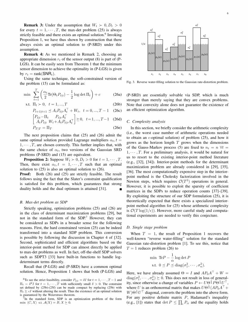
D. Single stage problem

When T = 1, the result of Proposition 1 recovers thewell-known “reverse water-filling” solution for the standardGaussian rate-distortion problem [1]. To see this, notice thatT = 1 reduces problem (26) to

min TrP − 1

αlog detP

s.t. 0 P diag(σ21 , · · · , σ2

n).

Here, we have already assumed Θ = I and AP0A> + W =

diag(σ21 , · · · , σ2

n) 0. This does not result in loss of general-ity, since otherwise a change of variables P ← UΘ

12PΘ

12U>,

where U is an orthonormal matrix that makes UΘ12 (AP0A

>+W )Θ

12U> diagonal, converts the problem into the above form.

For any positive definite matrix P , Hadamard’s inequality(e.g., [1]) states that detP ≤

∏i Pii and the equality holds

7

0 200 400 600 800 10000

5

10

15

20

Rank (

Num

ber

of sin

gula

r valu

es o

f

CTV

−1C

gre

ate

r th

an 1

0−

5)

(a) rank(CTV

−1C) and R

SRD

0 200 400 600 800 10000

20

40

60

80

Rate

, R

SR

D [bit/s

am

ple

]

Distortion, D

0 5 10 15 200

20

40

D=

1

(b) Singular values of CTV

−1C

0 5 10 15 200

0.02

0.04

D=

500

0 5 10 15 200

0.005

0.01

D=

1000

Rank

Rate, RSRD

Fig. 4. Numerical experiments on rank monotonicity. 20 dimensional Gaus-sian process is randomly generated and SNR = C>V −1C is constructedfor various D. Observe rank(SNR) tends to decrease as D increase.

if and only if the matrix is diagonal. Hence, if diagonalelements of P are fixed, detP is maximized by setting alloff-diagonal entries zero. Thus, the optimal solution to theabove problem is diagonal. Writing P = diag(p1, · · · , pn),the problem is decomposed as n independent optimizationproblems, each of which minimizes pi − 1

α log pi subject to0 ≤ pi ≤ σ2

i . It is easy to see that the optimal solution ispi = min(1/α, σ2

i ). This is the closed-form solution to (P-LGS) with T = 1, and its pictorial interpretation is shown inFig. 3. This solution also indicates the optimal sensing formulais given by y = Cx+v,v ∼ N (0, V ), where C and V satisfy

C>V −1C = P−1 − (AP0A> +W )−1

= diag1≤i≤n

(max

0, α− 1

σ2i

).

In particular, we have dim(y) = rank(C>V −1C) = cardi :σ2i >

1α, indicating that the optimal dimension of y monoton-

ically decreases as the “price of information” 1/α increases.

V. STATIONARY PROBLEMS

A. Sequential rate-distortion function

We are often interested in infinite-horizon Gaussian SRDproblems (13). Assuming that (A,Θ) is a detectable pair, itcan be shown that (13) is equivalent to the infinite-horizonlinear-Gaussian sensor design problem (14) [40]. Moreover,[40] shows that (13) and (14) admit an optimal solution thatcan be realized as a composition of a time-invariant sensormechanism yt = Cxt + vt with i.i.d. process vt ∼ N (0, V )and a time-invariant Kalman filter. Hence, it is enough tominimize the average cost per stage, which leads to thefollowing simpler problem.

RSRD(D) = min − 1

2log det Π +

1

2log detW (27a)

s.t. Π 0 (27b)

P APA> +W (27c)Tr(ΘP ) ≤ D (27d)[P −Π PA>

AP APA> +W

] 0. (27e)

To confirm (27) is compatible with the existing result, considera scalar system with A = a,W = w,P = p and Θ = 1. In

this case, a closed-form expression of the SRD function isknown in the literature [12] [16], which is given by

RSRD(D) = min

0,

1

2log(a2 +

w

D)

. (28)

For a scalar system, (27) further simplifies to

min log(a2 +w

p) (29a)

s.t. 0 < p ≤ a2p+ w, p ≤ D. (29b)

It is elementary to verify that the optimal value of (29) islog(a2 + w

D ) if 1− wD ≤ a

2, while it is 0 if 0 ≤ a2 < 1− wD .

Hence, it can be compactly written as min0, 12 log(a2 + w

D ),and the result recovers (28). Alternative representations of theSRD function (27) for stationary multi-dimensional Gauss-Markov processes when Θ = I are reported in [13, SectionIV-B] and [17, Section VI].

B. Rank monotonicity

Using an optimal solution to (27) the optimal sensingmatrices C and V are recovered from C>V −1C = P−1 −(APA> + W )−1. In particular, dim(y) = rank(C>V −1C)determines the optimal dimension of the measurement vector.Similarly to the case of single stage problems, this rank hasa tendency to decrease as D increases. A typical numericalbehavior is shown in Figure 4. We do not attempt to prove therank monotonicity here.

VI. APPLICATIONS AND RELATED WORKS

A. Zero-delay source coding

SRD theory plays an important role in the rate analysis ofzero-delay source coding schemes. For each t = 1, 2, · · · , let

Bt ⊂ 0, 1, 00, 01, 10, 11, 000, · · ·

be a set of variable-length uniquely decodable codewords.Assume that bt ∈ Bt for t = 1, 2, · · · , and let lt be the lengthof bt. A zero-delay binary coder is a pair of a sequence ofencoders et(dbt|xt, bt−1), i.e., stochastic kernels on Bt givenX t × Bt−1, and a sequence of decoders dt(dzt|bt, zt−1), i.e.,stochastic kernels on Zt given Bt × Zt−1. The zero-delayrate-distortion region for the Gauss-Markov process (12) isthe epigraph of the function

RopSRD(D) = inf

Bt,et,dt∞t=1

lim supT→∞

1

T

T∑t=1

E(lt)

s.t. lim supT→∞

1

T

T∑t=1

E‖xt − zt‖2Θ ≤ D.

The SRD function is a lower bound of the achievable rate.Indeed, RSRD(D) ≤ Rop

SRD(D) ∀D > 0 can be shown

8

straightforwardly as

I(xT → zT ) = I(xT ; zT ) (30a)

≤ I(xT ;bT ) (30b)

= H(bT )−H(bT |xT ) (30c)

≤ H(bT ) (30d)

≤∑T

t=1H(bt) (30e)

≤∑T

t=1E(lt) (30f)

where (30a) holds since there is no feedback from the pro-cess zt to xt (Remark 1), (30b) follows from the dataprocessing inequality, (30d) holds since conditional entropy isnon-negative, and (30e) is due to the chain rule for entropy.The final inequality (30f) holds since the expected length of auniquely decodable code is lower bounded by its entropy [1,Theorem 5.3,1].

In general, RSRD(D) and RopSRD(D) do not coincide. Never-

theless, by constructing an appropriate entropy-coded ditheredquantizer (ECDQ), it is shown in [16] that Rop

SRD(D) does notexceed RSRD(D) more than a constant due to the “space-fillingloss” of the lattice quantizer and the loss of entropy coding.

B. Networked control theory

Zero-delay source/channel coding technologies are crucialin networked control systems [41]–[44]. Gaussian SRD theoryplays an important role in the LQG control problems withinformation theoretic constraints [13]. It is shown in [19] thatan LQG control problem in which observed data must betransmitted to the controller over a noiseless binary channelis closely related to the LQG control problem with directedinformation constraints. The latter problem is addressed in[27] using the SDP-based algorithm presented in this paper. In[27], the problem is viewed as a sensor-controller joint designproblem in which directed information from the state processto the control input is minimized.8

C. Experimental design/Sensor scheduling

In this subsection, we compare the linear-Gaussian sensordesign problem (P-LGS) with different types of sensor de-sign/selection problems considered in the literature.

A problem of selecting the best subset of sensors to observea random variable in order to minimize the estimation errorand its convex relaxations are considered in [29]. A sensorselection problem for a linear dynamical system is consid-ered in [47], where submodularity of the objective functionis exploited. Dynamic sensor scheduling problems are alsoconsidered in the literature. In [48], an efficient algorithmto explore branches of the scheduling tree is proposed. In[49], a stochastic sensor selection strategy that minimizes theexpected error covariance is considered.

The linear-Gaussian sensor design problem (P-LGS) isdifferent from these sensor selection/scheduling problems inthat it is essentially a continuous optimization problem (since

8The problem considered in [27] is different from the sensor-controller jointdesign problems considered in [45] and [46].

10−3

10−2

10−1

100

0

0.2

0.4

0.6

0.8

1

Distortion, D

Rate

, R

SR

D (

D)

[b

its/s

am

ple

]

D=0.002R=0.3829

D=0.03R=0.0802

D=0.3R=0.0089

Fig. 5. Sequential rate-distortion function for the noisy double pendulum.

0 500 1000−0.5

0

0.5D=0.002 ( 0.3829 bits/sample )

θ1

0 500 1000−1

−0.5

0

0.5

1

θ2

0 500 1000−0.5

0

0.5D=0.03 ( 0.0802 bits/sample )

0 500 1000−1

−0.5

0

0.5

1

0 500 1000−0.5

0

0.5D=0.3 ( 0.0089 bits/sample )

0 500 1000−1

−0.5

0

0.5

1

State Estimated state

Fig. 6. Tracking performance of the Kalman filter under different distortionconstraints. (Tested on the same sample path of the noisy double pendulum.)

matrices Ct, VtTt=1 can be freely chosen), and the objectiveis to minimize an information-theoretic cost (11a).

VII. NUMERICAL SIMULATIONS

In this section, we consider two numerical examples todemonstrate how the SDP-based formulation of the GaussianSRD problem can be used to calculate the minimal commu-nication bandwidth required for the real-time estimation withdesired accuracy.

A. Optimal sensor design for double pendulumA linearized equation of motion of a double pendulum with

friction and disturbance is given bydθ1

dθ2

dω1

dω2

=

0 0 1 00 0 0 1

− (m1+m2)gm1l1

m2gm1l1

−c1 0(m1+m2)gm1l2

− (m1+m2)gm1l2

0 −c2

θ1

θ2

ω1

ω2

dt+dbwhere b is a Brownian motion. We consider a discrete timemodel of the above equation of motion obtained through theTustin transformation. We are interested in designing a sensingmodel yt = Cxt+vt,vt ∼ N (0, V ) that optimally trades-offinformation cost and distortion level.9 We solve the stationary

9In practice, it is often the case that xt is partially observable through agiven sensor mechanism. In such cases, the framework discussed in this paperis not appropriate. Instead, one can formulate an SRD problem for partiallyobservable Gauss-Markov processes. See [50] for details.

9

optimization problem (27) for this example with various valuesof D. The result is the sequential rate-distortion functionshown in Figure 5. Finally, for every point on the trade-offcurve, the optimal sensing matrices C and V are reconstructed,and the Kalman filter is designed base on them. Figure6 shows the trade-off between the distortion level and thetracking performance of the Kalman filter. When the distortionconstraint is strict (D = 0.002), the optimally designed sensorgenerates high rate information (0.3829 bits/sample) and theKalman filter built on it tracks true state very well. When Dis large (D = 0.3), the optimal sensing strategy chooses “notto observe much”, and the resulting Kalman filter shows poortracking performance.

B. Minimum down-link bandwidth for satellite attitude deter-mination

The equation of motion of the angular velocity vector of aspin-stabilized satellite linearized around the nominal angularvelocity vector (ω0, 0, 0) is dω1

dω2

dω3

=

1 0 00 1 I3−I1

I2ω0

0 I1−I2I3

ω0 1

ω1

ω2

ω3

dt+ db

where b is a disturbance. Again, the equation of motion isconverted to a discrete time model in the simulation. Supposethat the satellite has on-board sensors that can accuratelymeasure angular velocities, and the ground station needs toestimate them with some required accuracy (distortion) basedon the transmitted data from the satellite. Our interest isto determine the minimum down-link bit-rate that makes itpossible, and identify what information needs to be transmittedto achieve this. Assume that the distortion constraints Dt aretime varying, but given a priori. (For instance, it must be keptsmall only when the satellite is in a mission.) The discussionso far indicates that the data to be transmitted is in the formof yt = Ctxt + vt in order to minimize communication costmeasured by

∑Tt=1 I(xt,yt|yt−1). In Figure 7, a result of the

SDP (26) is plotted, when the scheduling horizon is T = 120and a particular distortion constraint profile Dt is given (shownin red in (a)). The optimal down-link schedule shown in (b)requires no communication at all when the distortion constraintis met. As by-products of the SDP (26), the optimal schedulingof sensing matrices Ct and noise covariances Vt of vt can bealso explicitly obtained.

VIII. CONCLUSION

In this paper, we revisited the “sensor-estimator separationprinciple” and showed that an optimal solution to the GaussianSRD problem can be found by considering a related linear-Gaussian sensor design problem, which can be formulated asa determinant maximization problem with LMI constraints.The implication is that Gaussian SRD problems are efficientlysolvable using standard SDP solvers. We have also consideredseveral potential applications of the Gaussian SRD problemand its relationship to real-time communication theory, net-worked control theory, and sensor scheduling problems.

0 20 40 60 80 100 1200

0.5

1

x 10−3 (a) Distortion constraint ( D t ) and optimal covariance scheduling ( Trace P t | t )

0 20 40 60 80 100 1200

2

4

6(b) Optimal information rate, I ( x t ; y t | y

t−1 )

Time [ min ]

D t Trace P t | t

Fig. 7. Satellite attitude determination with time-varying distortion con-straints.

APPENDIX AMATHEMATICAL PRELIMINARIES

A. Stochastic kernels

Let X ,Y be Euclidean spaces. A (Borel-measurable)stochastic kernel on Y given X is a map qy|x : BY×X → [0, 1]such that qy|x(·|x) is a probability measure on (Y,BY) forevery x ∈ X , and qy|x(A|·) is a Borel measurable functionfor every A ∈ BY . For simplicity, a stochastic kernel on Ygiven X will be denoted by q(dy|x). The following resultscan be found in Propositions 7.27 and 7.28 in [51].

Lemma 3: Let X ,Y be Euclidean spaces.

(a) Let r be a probability measure on (X ,BX ), and q(dy|x)be a Borel measurable stochastic kernel on Y given X .Then, there exists a unique probability measure p on(X × Y,BX×Y) such that

p(BX×BY )=

∫BX

q(BY |x)r(dx) ∀BX ∈BX , BY ∈BY .(31)

(b) Let p be a probability measure on (X × Y,BX×Y). Thenthere exists a Borel-measurable stochastic kernel q(dy|x) onY given X such that (31) holds, where r is the marginal ofp on X .

Lemma 3 (a) guarantees the function p defined on the algebraof measurable rectangles by (31) has a unique extension to theσ-algebra BX×Y . For simplicity, the joint probability measuredefined this way is denoted by

p(dx, dy) = q(dy|x)r(dx). (32)

Conversely, if the left hand side of (32) is given, Lemma 3(b) guarantees the existence of the decomposition on the righthand side.

Definition 1: A stochastic kernel q(dzT |xT ) on ZT givenX T is said to be zero-delay if it admits a factorizationq(dzT |xT ) =

∏Tt=1 q(dzt|zt−1, xt).

Once a zero-delay stochastic kernel is specified, successive ap-plications of Lemma 3 (a) uniquely determine a joint probabil-ity measure by q(dxT , dzT ) = q(dxT )

∏Tt=1 q(dzt|zt−1, xt).

The mutual information and the expectation in (P-SRD) isunderstood with respect to this joint probability measure.

10

Let p and q be probability measures on X = Rn. Wheneverp is absolutely continuous with respect to q (denoted by pq), dpdq denotes the Radon-Nikodym derivative.

Lemma 4: Let X and Y be Polish spaces.(a) If p, q, r are probability measures on X such that r q

and q p, then r p and drdp = dr

dqdqdp p− a.e.. If q p

and p q, then dpdq

dqdp = 1 a.e..

(b) Let px,y be a joint probability measure on X×Y , and px, pybe its marginals. Let px|y be a Borel-measurable stochastickernel such that

px,y(BX ×BY ) =

∫BY

px|y(BX |y)py(dy) (33)

for every BX ∈ BX , BY ∈ BY . If px,y px × py, then

dpx,yd(px × py)

=dpx|y

dpxpy − a.e.. (34)

Proof: For (a), see Proposition 3.9 in [52]. To prove (b), letf(x, y) =

dpx,y

d(px×py) . By definition,

px,y(BX ×BY ) =

∫BX×BY

f(x, y)(px × py)(dx, dy)

=

∫BY

(∫BX

f(x, y)px(dx)

)py(dy)

Since clearly f ∈ L1(px × py), the Fubini’s theorem [52] isapplicable in the second line. Substituting this expression into(33), we have

∫BX

f(x, y)px(dx) = px|y(BX |y) py − a.e..

Thus f(x, y) =dpx|ydpx

py − a.e..

B. Information theoretic quantities

The relative entropy, also known as the Kullback–Leiblerdivergence, from p to q is defined by

DKL(p‖q) =

∫log dp

dqdq if p q

+∞ otherwise.

Relative entropy is always nonnegative. Given two stochastickernels px|y(dx|y) and qx|y(dx|y) on X given Y , and aprobability measure ry(dy), the conditional relative entropyis defined by

DKL(px|y‖qx|y|ry)=

∫YDKL(px|y(dx|y)‖qx|y(dx|y))ry(dy).

Suppose X ,Y,Z are Euclidean spaces, and qx,y is a jointprobability measure on X × Y . Let qx, qy be its marginals,and qx × qy be the product measure. The mutual informationbetween x and y is defined by I(x;y) = DKL(qx,y||qx×qy).Given a joint probability measure q(dx, dy, dz), the condi-tional mutual information is defined by

I(x;y|z) = DKL(qx,y|z‖qx|y × qy|z|qz).

Suppose X = Rn, and x is a (X ,BX )-valued random variablewith probability measure qx. Let λ be the Lebesgue measureon X restricted to BX . The differential entropy of x is definedby

h(x) =

−∫

log dqxdλ dqx if qx λ

−∞ otherwise.

APPENDIX BPROOF OF LEMMA 1

(i): Given a sequence of stochastic kernels γ =⊗Tt=1q(dzt|xt, zt−1) ∈ Γ attaining cost fSRD < +∞ in(P-SRD), we are going to construct a sequence of linear-Gaussian stochastic kernels of the form (16) that incurs nogreater cost than fSRD in (P-1). Let q(dxT , dzT ) be the jointprobability measure generated by γ and the underlying Gauss-Markov process (5). Without loss of generality, we can assumeq(dxT , dzT ) has zero-mean. Otherwise, it is possible to choosean alternative feasible policy γ ∈ Γ by linearly shifting γ sothat the resulting probability measure q(dxT , dzT ) has zero-mean. This operation does not increase the mutual informationterms in the objective function.

Let r(dxT , dzT ) be a zero-mean, jointly Gaussian proba-bility measure with the same covariance as q(dxT , dzT ). LetEtxt+Ft,t−1zt−1+· · ·+Ft,1z1 be the least mean square errorestimate of zt given xt, z

t−1 in r(dxT , dzT ), and let Γt be thecovariance matrix of the corresponding estimation error. Letgt be a sequence of Gaussian random vectors such that gtis independent of x0,w

t,gt−1 and gt ∼ N (0,Γt). For everyt = 1, · · · , T , define a stochastic kernel s(dzt|xt, zt−1) by

zt = Etxt + Ft,t−1zt−1 + · · ·+ Ft,1z1 + gt.

We set γ1 = ⊗Tt=1s(dzt|xt, zt−1) ∈ Γ1 as a candidate solutionto (P-1). By construction of s(dzt|xt, zt−1), the followingrelation holds for every t = 1, · · · , T :

r(dxt, dzt) = s(dzt|xt, zt−1)r(dxt, dz

t−1). (35)

Let s(dxT , dzT ) be a jointly Gaussian measure defined bys(dzt|xt, zt−1)Tt=1 and the process (5). That is, it is a jointmeasure recursively defined by

s(dxt, dzt−1) = q(dxt|xt−1)s(dxt−1, dzt−1) (36a)

s(dxt, dzt) = s(dzt|xt, zt−1)s(dxt, dzt−1). (36b)

where q(dxt|xt−1) is a stochastic kernel defined by (5).Notice the following fact about r(dxT , dzT ).Proposition 3: For t = 2, · · · , T , let r(dxt−1, dz

t−1)and r(dxt−1, dxt, dz

t−1) be marginals of r(dxT , dzT ). Thenr(dxt−1, dxt, dz

t−1) = q(dxt|xt−1)r(dxt−1, dzt−1).

Proof: Since zt−1 – xt−1 – xt forms a Markov chainin the measure q(dxT , dzT ), by Lemma 3.2 of [53], zt−1

– xt−1 – xt forms a Markov chain under r(dxT , dzT )as well. Hence under r, xt is independent of zt−1 givenxt−1, or r(dxt|xt−1, z

t−1) = r(dxt|xt−1). Moreover, sinceq(dxt, dxt−1) is a Gaussian distribution, and since r is de-fined to be a Gaussian distribution with the same covari-ance as q, r(dxt, dxt−1) and q(dxt, dxt−1) have the samejoint distribution. Hence, q(dxt|xt−1) = r(dxt|xt−1). Thus,r(dxt|xt−1, z

t−1) = q(dxt|xt−1), proving the claim.

In general, r(dxT , dzT ) and s(dxT , dzT ) are different jointprobability measures. However, we have the following result.

Proposition 4: For every t = 1, · · · , T , let r(dxt, dzt)and s(dxt, dzt) be marginals of r(dxT , dzT ) and s(dxT , dzT )respectively. Then r(dxt, dzt) = s(dxt, dz

t).

11

Proof: By definitions,

r(dx1, dz1) = s(dz1|x1)r(dx1)

s(dx1, dz1) = s(dz1|x1)q(dx1).

Since r(dx1) = q(dx1), r(dx1, dz1) = s(dx1, dz1) holds. Soassume that the claim holds for t = k − 1. Then

s(dxk, dzk)

= s(dzk|xk, zk−1)s(dxk, dzk−1) (37a)

= s(dzk|xk, zk−1)

∫Xk−1

s(dxk−1, dxk, dzk−1)

= s(dzk|xk, zk−1)

∫Xk−1

q(dxk|xk−1)s(dxk−1, dzk−1) (37b)

= s(dzk|xk, zk−1)

∫Xk−1

q(dxk|xk−1)r(dxk−1, dzk−1) (37c)

= s(dzk|xk, zk−1)

∫Xk−1

r(dxk−1, dxk, dzk−1) (37d)

= s(dzk|xk, zk−1)r(dxk, dzk−1)

= r(dxk, dzk). (37e)

The first step (37a) follows from the definition (36b). Step(37b) also follows from the definition (36a). In (37c), theinduction assumption s(dxk−1, dz

k−1) = r(dxk−1, dzk−1)

was used. The result of Proposition 3 was used in (37d). Thefinal step (37e) is due to (35).

To prove that γ1 = ⊗Tt=1s(dzt|xt, zt−1) incurs no greatercost than fSRD in (P-1), notice that replacing q(dzt|xt, zt−1)with s(dzt|xt, zt−1) will not change the distortion:

Eq‖xt − zt‖2Θt=

∫‖xt − zt‖2Θt

q(dxt, dzt)

=

∫‖xt − zt‖2Θt

r(dxt, dzt) (38)

=

∫‖xt − zt‖2Θt

s(dxt, dzt) (39)

= Es‖xt − zt‖2Θt.

Equality (38) holds since q and r have the same second orderproperties. The result of Proposition 4 was used in step (39).

Next, we show that the mutual information never increasesby this replacement.

Proposition 5: If Iq(xT ; zT ) < +∞, then Ir(xT ; zT ) ≤

Iq(xT ; zT ).

Proof: This can be directly verified as

Iq(xT ; zT )− Ir(xT ; zT )

=

∫log

dq(xT |zT )

dq(xT )q(dxT , dzT ) (40)

−∫

logdr(xT |zT )

dr(xT )r(dxT , dzT ) (41)

=

∫log

dq(xT |zT )

dq(xT )q(dxT , dzT )

−∫

logdr(xT |zT )

dr(xT )q(dxT , dzT ) (42)

=

∫log

(dq(xT |zT )

dq(xT )· dr(xT )

dr(xT |zT )

)q(dxT , dzT )

=

∫log

(dq(xT |zT )

dr(xT |zT )

)q(dxT , dzT ) (43)

=

∫ (∫log

(dq(xT |zT )

dr(xT |zT )

)q(dxT |zT )

)q(dzT )

=

∫DKL

(q(xT |zT )||r(xT |zT )

)q(dzT ) ≥ 0.

(40) is by definition of mutual information and Lemma 4(b). Since q(dxT ) is a non-degenerate Gaussian probabilitymeasure, Iq(xT ; zT ) < +∞ implies that q(dxT |zT ) ad-mits a density q(dzT ) − a.e.. This further requires that aGaussian measure r(dxT |zT ) admits a density everywherein supp(r(dzT )), i.e., the support of the probability measurer(dzT ). Thus, the Radon-Nikodym derivative in (41) existseverywhere in supp(r(dzT )). Since r is a Gaussian probabilitymeasure, log dr(xT |zT )

dr(xT )is a quadratic function of xT and zT

everywhere in supp(r(dxT , dzT )). Since it can be shown thatsupp(q(dxT , dzT )) ⊆ supp(r(dxT , dzT )), this allows us toreplace r(dxT , dzT ) with q(dxT , dzT ) in (42) since they havethe same second order moments. Lemma 33 (a) is applicablein (43) since r(dxT ) = q(dxT ).

Finally,

∑T

t=1Iq(x

t; zt|zt−1) = Iq(xT ; zT ) (44)

≥ Ir(xT ; zT ) (45)

=∑T

t=1Ir(x

T ; zt|zt−1)

≥∑T

t=1Ir(xt; zt|zt−1)

=∑T

t=1Is(xt; zt|zt−1) (46)

See Remark 1 for the equality (44). The result of Proposition 5was used in (45). Equality (46) follows from Proposition 4.Thus, using γ = ⊗Tt=1q(dzt|xt, zt−1) ∈ Γ attaining cost fSRDin (P-SRD), we have constructed γ1 = ⊗Tt=1s(dzt|xt, zt−1) ∈Γ1 incurring smaller cost in (P-1) than fSRD.

(ii): Let γ1 = ⊗Tt=1q(dzt|xt, zt−1) ∈ Γ1 be a sequenceof linear-Gaussian stochastic kernels attaining f1 < +∞in (P-1), and q(dxT , dzT ) be the resulting joint probabilitymeasure. Since zt – (xt, z

t−1) – xt−1 forms a Markov chain

12

in q(dxT , dzT ), we have

I(xt; zt|zt−1) = I(xt; zt|zt−1) + I(xt−1; zt|xt, zt−1)

= I(xt; zt|zt−1). (47)

Hence the mutual information terms in (P-1) can be replacedwith the ones in (P-SRD) without increasing cost.

APPENDIX CPROOF OF LEMMA 2

(i): Suppose

zt=Etxt+Ft,t−1zt−1+· · ·+Ft,1z1+gt, t=1, · · ·, T (48)

is a linear-Gaussian stochastic kernel that attains f1 < +∞ in(P-1). It is sufficient for us to show that there exist nonnegativeintegers r1, · · · , rT and matrices Ct ∈ Rrt×nt , Vt ∈ Srt++, t =1, · · · , T such that Ct, VtTt=1 attains a smaller cost than f1

in (P-LGS). Let[U1 U2

] [ Σ1 00 0

] [U>1U>2

]= Egtg>t

with an orthonormal matrix U =[U1 U2

]be a singular

value decomposition of the covariance matrix of gt. If gt isnondegenerate, we understand that U = U1, while if gt is apoint mass at zero, then U = U2. Clearly gt = U>1 gt is a zero-mean, nondegenerate Gaussian random vector and U>2 gt = 0.Define[

ztzt

]=

[U>1U>2

]zt,

[EtEt

]=

[U>1U>2

]Et,

[Ft,sFt,s

]=

[U>1U>2

]Ft,s

for s = 1, · · · , t− 1. Then multiplying (48) by U> from theleft yields[

ztzt

]=

[EtEt

]xt+

[Ft,t−1

Ft,t−1

]zt−1+· · ·+

[Ft,1Ft,1

]z1+

[gt0

]. (49)

Proposition 6: Et = 0 ∀t = 1, · · · , T is necessary forf1 < +∞.Proof: Focus on the mutual information terms in (P-1).

I(xt; zt|zt−1)

= I(xt; zt, zt|zt−1)

≥ I(xt; zt|zt−1)

= I(xt; Etxt + Ft,t−1zt−1 + · · ·+ Ft,1z1|zt−1)

= I(xt; Etxt|zt−1)

= I(xt; Etxt, zt−1)− I(xt; z

t−1)

≥ I(xt; Etxt)− I(xt; zt−1)

Recall that xt is defined by (5) and is a nondegenerateGaussian random vector. If Etxt is a non-zero linear functionof xt, then I(xt; Etxt) = +∞, while I(xt; z

t−1) is bounded.Therefore, Et = 0 is necessary for I(xt; zt|zt−1) to bebounded.

Proposition 6, together with (49), implies that zt is a lin-ear function of zt−1. Hence, there exist some matrices

Ht,1, · · · , Ht,t−1 such that the first row of (49) can berewritten as

zt = Etxt +Ht,t−1zt−1 + · · ·+Ht,1z1 + gt. (50)

It is also easy to see that zt can be fully reconstructed if zt isgiven. In particular, this implies that the σ-algebras generatedby zt and zt are the same.

σ(zt) = σ(zt). (51)

Proposition 7: I(xt; zt|zt−1) = I(xt; zt|zt−1) ∀t =1, · · · , T .Proof: This can be directly verified as follows.

I(xt; zt|zt−1) = I(xt; zt, zt|zt−1)

= I(xt; zt|zt−1) (52)

= I(xt; zt|zt−1, zt−1, zt−2)

= I(xt; zt|zt−1, zt−2) (53)

= I(xt; zt|zt−1, zt−2, zt−3)

...

= I(xt; zt|zt−1)

Equality (52) holds since zt is a linear function of zt−1.Similarly, (53) holds because zt−1 is a linear function of zt−2.The remaining equalities can be shown by repeating the sameargument.

Now, for every t = 1, · · · , T , set Ct = Et and vt = gt. Then,by construction, vt is a zero-mean, nondegenerate Gaussianrandom vector that is independent of x0,w

t,vt−1. Henceyt = Ctxt+vt is an admissible sensor equation for (P-LGS).

Proposition 8: I(xt;yt|yt−1) = I(xt; zt|zt−1) ∀t =1, · · · , T .Proof: By concatenating (50), it can be easily seen that anidentity Htzt = yt holds for every t = 1, · · · , T , where Htis an invertible matrix defined by

Ht =

I 0 · · · 0

−H2,1 I. . .

......

. . . . . . 0−Ht,1 · · · −Ht,t−1 I

.Hence,

I(xt;yt|yt−1) = I(xt;yt|zt−1)

=I(xt; zt−Ht,t−1zt−1−· · ·−Ht,1z1|zt−1)

=I(xt; zt|zt−1).

Thus, starting from a sequence of linear-Gaussian stochastickernels (48), we have constructed a sequence of sensor equa-tions of the form yt = Ctxt + vt such that I(xt;yt|yt−1) =I(xt; zt|zt−1). The last equality is a consequence of Proposi-tions 7 and 8. To complete the proof of the first statement ofLemma 2, it is left to show that

E‖xt − z′t‖2Θt≤ E‖xt − zt‖2Θt

∀t = 1, · · · , T (54)

13

where z′t = E(xt|yt). (Here, we refer to the variable “zt” in(P-LGS) as z′t in order to distinguish it from the variable ztin (P-1).) The inequality (54) can be verified by the followingobservation. Since Htzt = yt, we have σ(yt) = σ(zt).Moreover, it follows from (51) that σ(yt) = σ(zt). Thus,zt is σ(yt)-measurable. However, since z′t = E(xt|yt), z′tminimizes the mean square estimation error among all σ(yt)-measurable functions. Thus (54) must hold.

(ii): Let Ct, VtTt=1 be a sequence of matrices that attainsfLGS < +∞ in (P-LGS). Let yt be defined by (8), and z′t =E(xt|yt) be the least mean square error estimate of xt givenyt obtained by the Kalman filter. From the Kalman filteringformula, we have

z′t=At−1z′t−1+Pt|t−1C

>t (CtPt|t−1C

>t +Vt)

−1(yt−CtAt−1z′t−1)

=Etxt + Ft,t−1z′t−1 + · · ·+ Ft,1z

′1 + gt

where Et, Ft,t−1, · · · , Ft,1 are some matrices (in fact, allFt,t−2, · · · , Ft,1 are zero matrices) and gt is a zero-meanGaussian random vector that is independent of x0,w

t andgt−1. Hence, by constructing a linear-Gaussian stochastickernel for (P-1) by

zt = Etxt + Ft,t−1zt−1 + · · ·+ Ft,1z1 + gt

using the same Et, Ft,t−1, · · · , Ft,1 and gt, (xT , zT ) and(xT , z′T ) have the same joint distribution. Thus E‖xt −z′t‖2Θt

= E‖xt − zt‖2Θt∀t = 1, · · · , T . Hence, it remains

to prove that

I(xt;yt|yt−1) ≥ I(xt; zt|zt−1) ∀t = 1, · · · , T.

Notice that I(xt;yt|zt−1) ≥ I(xt; zt|zt−1) is immediatefrom the data-processing inequality. Moreover, an equalityI(xt;yt|yt−1) = I(xt;yt|zt−1) holds since the input se-quence yt−1 and the output sequence zt−1 of the Kalmanfilter contain statistically equivalent information. Formally, thiscan be shown by proving that the Kalman filter is causallyinvertible [54], and thus one can construct yt−1 from zt−1

and vice versa.

ACKNOWLEDGMENT

The authors would like to thank Prof. Sekhar Tatikonda forvaluable discussions.

REFERENCES

[1] T. M. Cover and J. A. Thomas, Elements of Information Theory. NewYork, NY, USA: Wiley-Interscience, 1991.

[2] N. T. Gaarder and D. Slepian, “On optimal finite-state digital transmis-sion systems,” IEEE Transactions on Information Theory, vol. 28, no. 2,pp. 167–186, 1982.

[3] H. Witsenhausen, “On the structure of real-time source coders,” BellSystem Technical Journal, The, vol. 58, no. 6, pp. 1437–1451, 1979.

[4] D. L. Neuhoff and R. K. Gilbert, “Causal source codes,” IEEE Trans-actions on Information Theory, vol. 28, no. 5, pp. 701–713, 1982.

[5] T. Linder and R. Zamir, “Causal coding of stationary sources andindividual sequences with high resolution,” IEEE Transactions on In-formation Theory, vol. 52, no. 2, pp. 662–680, 2006.

[6] S. Yuksel, “On optimal causal coding of partially observed markovsources in single and multiterminal settings,” IEEE Transactions onInformation Theory, vol. 59, no. 1, pp. 424–437, 2013.

[7] V. Kostina and S. Verdu, “Fixed-length lossy compression in the finiteblocklength regime,” Information Theory, IEEE Transactions on, vol. 58,no. 6, pp. 3309–3338, 2012.

[8] J. C. Walrand and P. Varaiya, “Optimal causal coding-decoding prob-lems,” IEEE Transactions on Information Theory, vol. 29, no. 6, pp.814–820, 1983.

[9] D. Teneketzis, “On the structure of optimal real-time encoders anddecoders in noisy communication,” IEEE Transactions on InformationTheory, vol. 52, no. 9, pp. 4017–4035, 2006.

[10] A. Mahajan and D. Teneketzis, “Optimal design of sequential real-timecommunication systems,” IEEE Transactions on Information Theory,vol. 55, no. 11, pp. 5317–5338, 2009.

[11] S. K. Gorantla and T. P. Coleman, “Information-theoretic viewpoints onoptimal causal coding-decoding problems,” CoRR, vol. abs/1102.0250,2011.

[12] S. Tatikonda, “Control under communication constraints,” PhD thesis,Massachusetts Institute of Technology, 2000.

[13] S. Tatikonda, A. Sahai, and S. Mitter, “Stochastic linear control overa communication channel,” IEEE Transactions on Automatic Control,vol. 49, no. 9, pp. 1549–1561, 2004.

[14] A. Gorbunov and M. Pinsker, “Nonanticipatory and prognostic epsilonentropies and message generation rates,” Problemy Peredachi Informat-sii, vol. 9, no. 3, pp. 12–21, 1973.

[15] R. Bucy, “Distortion-rate theory and filtering,” in Advances in Commu-nications. Springer, 1980, pp. 11–15.

[16] M. S. Derpich and J. Ostergaard, “Improved upper bounds to the causalquadratic rate-distortion function for Gaussian stationary sources,” IEEETransactions on Information Theory, vol. 58, no. 5, pp. 3131–3152,2012.

[17] C. D. Charalambous, P. Stavrou, N. U. Ahmed et al., “Nonanticipativerate distortion function and relations to filtering theory,” IEEE Transac-tions on Automatic Control, vol. 59, no. 4, pp. 937–952, 2014.

[18] J. Massey, “Causality, feedback and directed information,” InternationalSymposium on Information Theory and Its Applications (ISITA), pp.303–305, 1990.

[19] E. I. Silva, M. S. Derpich, and J. Ostergaard, “A framework for con-trol system design subject to average data-rate constraints,” AutomaticControl, IEEE Transactions on, vol. 56, no. 8, pp. 1886–1899, 2011.

[20] G. Blekherman, P. Parrilo, and R. Thomas, Semidefinite Optimizationand Convex Algebraic Geometry, ser. MOS-SIAM Series on Optimiza-tion. Society for Industrial and Applied Mathematics, 2013.

[21] T. E. Duncan, “On the calculation of mutual information,” SIAM Journalon Applied Mathematics, vol. 19, no. 1, pp. 215–220, 1970.

[22] D. Guo, S. Shamai, and S. Verdu, “Mutual information and minimummean-square error in Gaussian channels,” IEEE Transactions on Infor-mation Theory, vol. 51, no. 4, pp. 1261–1282, 2005.

[23] T. Weissman, Y.-H. Kim, and H. H. Permuter, “Directed information,causal estimation, and communication in continuous time,” IEEE Trans-actions on Information Theory, vol. 59, no. 3, pp. 1271–1287, 2013.

[24] F. Rezaei, N. Ahmed, and C. D. Charalambous, “Rate distortion theoryfor general sources with potential application to image compression,”International Journal of Applied Mathematical Sciences, vol. 3, no. 2,pp. 141–165, 2006.

[25] H. Marko, “The bidirectional communication theory–a generalization ofinformation theory,” IEEE Transactions on Communications, vol. 21,no. 12, pp. 1345–1351, 1973.

[26] J. L. Massey and P. C. Massey, “Conservation of mutual and directedinformation,” in Proceedings. International Symposium on InformationTheory, 2005. IEEE, 2005, pp. 157–158.

[27] T. Tanaka and H. Sandberg, “SDP-based joint sensor and controllerdesign for information-regularized optimal LQG control,” 54th IEEEConference on Decision and Control (CDC), 2015.

[28] D. P. Bertsekas, Nonlinear Programming. Athena Scientific, 1995.[29] L. Vandenberghe, S. Boyd, and S.-P. Wu, “Determinant maximization

with linear matrix inequality constraints,” SIAM journal on matrixanalysis and applications, vol. 19, no. 2, pp. 499–533, 1998.

[30] D. A. Harville, Matrix algebra from a statistician’s perspective.Springer, 1997, vol. 1.

[31] S. Boyd and L. Vandenberghe, Convex Optimization. New York, NY,USA: Cambridge University Press, 2004.

[32] A. Ben-Tal and A. Nemirovski, Lectures on modern convex optimization:Analysis, algorithms, and engineering applications. Philadelphia, PA,USA: SIAM, 2001, vol. 2.

[33] R. H. Tutuncu, K. C. Toh, and M. J. Todd, “Solving semidefinite-quadratic-linear programs using SDPT3,” Mathematical programming,vol. 95, no. 2, pp. 189–217, 2003.

[34] J. Renegar, A mathematical view of interior-point methods in convexoptimization. Philadelphia, PA, USA: SIAM, 2001, vol. 3.

14

[35] K.-C. Toh, “Primal-dual path-following algorithms for determinantmaximization problems with linear matrix inequalities,” ComputationalOptimization and Applications, vol. 14, no. 3, pp. 309–330, 1999.

[36] T. Tsuchiya and Y. Xia, “An extension of the standard polynomial-time primal-dual path-following algorithm to the weighted determinantmaximization problem with semidefinite constraints,” Pacific Journal ofOptimization, vol. 3, no. 1, pp. 165–182, 2007.

[37] M. Fukuda, M. Kojima, K. Murota, and K. Nakata, “Exploiting sparsityin semidefinite programming via matrix completion I: General frame-work,” SIAM Journal on Optimization, vol. 11, no. 3, pp. 647–674,2001.

[38] K. Nakata, K. Fujisawa, M. Fukuda, M. Kojima, and K. Murota,“Exploiting sparsity in semidefinite programming via matrix completionII: Implementation and numerical results,” Mathematical Programming,vol. 95, no. 2, pp. 303–327, 2003.

[39] L. Vandenberghe and M. Andersen, Chordal Graphs and SemidefiniteOptimization. Now Publishers Incorporated, 2015.

[40] T. Tanaka, “Semidefinite representation of sequential rate-distortionfunction for stationary Gauss-Markov processes,” IEEE Multi-Conference on Systems and Control (MSC), 2015.

[41] G. N. Nair, F. Fagnani, S. Zampieri, and R. J. Evans, “Feedback controlunder data rate constraints: An overview,” Proceedings of the IEEE,vol. 95, no. 1, pp. 108–137, 2007.

[42] J. Baillieul and P. J. Antsaklis, “Control and communication challengesin networked real-time systems,” Proceedings of the IEEE, vol. 95, no. 1,pp. 9–28, 2007.

[43] J. P. Hespanha, P. Naghshtabrizi, and Y. Xu, “A survey of recent resultsin networked control systems,” Proceedings of the IEEE, vol. 95, no. 1,p. 138, 2007.

[44] S. Yuksel and T. Basar, Stochastic networked control systems, ser.Systems & Control Foundations & Applications. New York, NY:Springer, 2013, vol. 10.

[45] R. Bansal and T. Basar, “Simultaneous design of measurement andcontrol strategies for stochastic systems with feedback,” Automatica,vol. 25, no. 5, pp. 679–694, 1989.

[46] B. M. Miller and W. J. Runggaldier, “Optimization of observations: astochastic control approach,” SIAM journal on control and optimization,vol. 35, no. 3, pp. 1030–1052, 1997.

[47] T. Summers, F. Cortesi, and J. Lygeros, “On submodularity and control-lability in complex dynamical networks,” IEEE Transactions on Controlof Network Systems, vol. PP, no. 99, 2015.

[48] M. P. Vitus, W. Zhang, A. Abate, J. Hu, and C. J. Tomlin, “On efficientsensor scheduling for linear dynamical systems,” Automatica, vol. 48,no. 10, pp. 2482–2493, 2012.

[49] V. Gupta, T. H. Chung, B. Hassibi, and R. M. Murray, “On a stochasticsensor selection algorithm with applications in sensor scheduling andsensor coverage,” Automatica, vol. 42, no. 2, pp. 251–260, 2006.

[50] T. Tanaka, “Zero-delay rate-distortion optimization for partially observ-able gauss-markov processes,” 54th IEEE Conference on Decision andControl (CDC), 2015.

[51] D. P. Bertsekas and S. E. Shreve, Stochastic optimal control: The discretetime case. Academic Press New York, 1978, vol. 139.

[52] G. Folland, Real analysis: Modern techniques and their applications.Hoboken, NJ, USA: John Wiley & Sons, 1999.

[53] Y.-H. Kim, “Feedback capacity of stationary Gaussian channels,” IEEETransactions on Information Theory, vol. 56, no. 1, pp. 57–85, 2010.

[54] T. Kailath, “An innovations approach to least-squares estimation – Part I:Linear filtering in additive white noise,” IEEE Transactions on AutomaticControl, vol. 13, no. 6, pp. 646–655, 1968.