Model predictive control without terminal constraints: stability and performance Lars Gr¨ une Mathematisches Institut, Universit¨ at Bayreuth in collaboration with Anders Rantzer (Lund), Nils Altm¨ uller (Bayreuth), Thomas Jahn (Bayreuth), J¨ urgen Pannek (Perth), Karl Worthmann (Bayreuth) supported by DFG priority research program 1305 and Marie-Curie ITN SADCO SontagFest’11, DIMACS, Rutgers, May 23–25, 2011
Transcript
Model predictive control without terminal
constraints: stability and performance
Lars Grune
Mathematisches Institut, Universitat Bayreuth
in collaboration with
Anders Rantzer (Lund), Nils Altmuller (Bayreuth), Thomas Jahn (Bayreuth),Jurgen Pannek (Perth), Karl Worthmann (Bayreuth)
supported by DFG priority research program 1305 and Marie-Curie ITN SADCO
SontagFest’11, DIMACS, Rutgers, May 23–25, 2011
Happy 60th Birthday Eduardo!
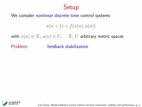
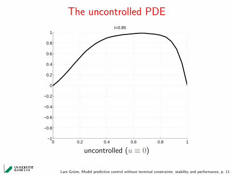
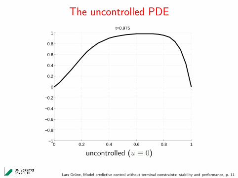
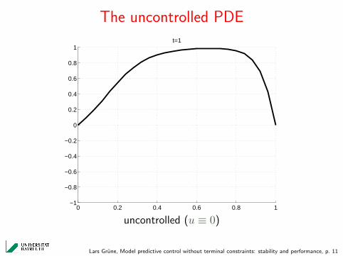
SetupWe consider nonlinear discrete time control systems
x(n+ 1) = f(x(n), u(n))
with x(n) ∈ X, u(n) ∈ U , X, U arbitrary metric spaces
Problem: Optimal feedback stabilization via infinite horizonoptimal control:
For a running cost ` : X × U → R+0 penalizing the distance to
the desired equilibrium solve
minimize J∞(x, u) =∞∑
n=0
`(x(n), u(n)) with u(n) = F (x(n)),
subject to state/control constraints x ∈ X, u ∈ U
Lars Grune, Model predictive control without terminal constraints: stability and performance, p. 2
SetupWe consider nonlinear discrete time control systems
x(n+ 1) = f(x(n), u(n))
with x(n) ∈ X, u(n) ∈ U , X, U arbitrary metric spaces
Problem:
Optimal
feedback stabilization
via infinite horizonoptimal control:
For a running cost ` : X × U → R+0 penalizing the distance to
the desired equilibrium solve
minimize J∞(x, u) =∞∑
n=0
`(x(n), u(n)) with u(n) = F (x(n)),
subject to state/control constraints x ∈ X, u ∈ U
Lars Grune, Model predictive control without terminal constraints: stability and performance, p. 2
SetupWe consider nonlinear discrete time control systems
x(n+ 1) = f(x(n), u(n))
with x(n) ∈ X, u(n) ∈ U , X, U arbitrary metric spaces
Problem: Optimal feedback stabilization via infinite horizonoptimal control:
For a running cost ` : X × U → R+0 penalizing the distance to
the desired equilibrium solve
minimize J∞(x, u) =∞∑
n=0
`(x(n), u(n)) with u(n) = F (x(n))
,
subject to state/control constraints x ∈ X, u ∈ U
Lars Grune, Model predictive control without terminal constraints: stability and performance, p. 2
SetupWe consider nonlinear discrete time control systems
x(n+ 1) = f(x(n), u(n))
with x(n) ∈ X, u(n) ∈ U , X, U arbitrary metric spaces
Problem: Optimal feedback stabilization via infinite horizonoptimal control:
For a running cost ` : X × U → R+0 penalizing the distance to
the desired equilibrium solve
minimize J∞(x, u) =∞∑
n=0
`(x(n), u(n)) with u(n) = F (x(n)),
subject to state/control constraints x ∈ X, u ∈ U
Lars Grune, Model predictive control without terminal constraints: stability and performance, p. 2
Model predictive controlDirect solution of the problem is numerically hard
Alternative method: model predictive control (MPC)
Idea: replace the original problem
minimize J∞(x, u) =∞∑
n=0
`(x(n), u(n))
by the iterative (online) solution of finite horizon problems
minimize JN(x, u) =N−1∑k=0
`(xu(k), u(k))
with xu(k) ∈ X, u(k) ∈ U
We obtain a feedback law FN by a moving horizon technique
Lars Grune, Model predictive control without terminal constraints: stability and performance, p. 3
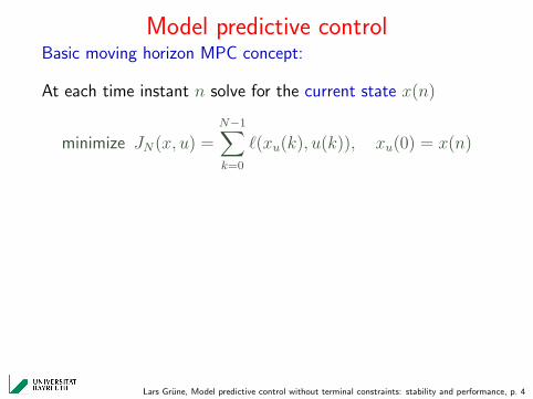
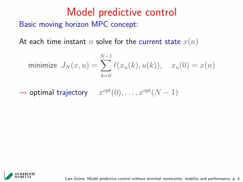
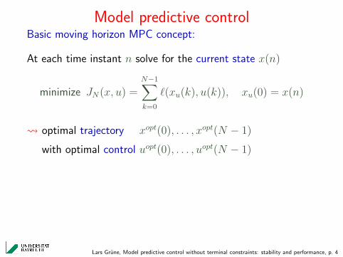
Model predictive controlBasic moving horizon MPC concept:
At each time instant n solve for the current state x(n)
Lars Grune, Model predictive control without terminal constraints: stability and performance, p. 4
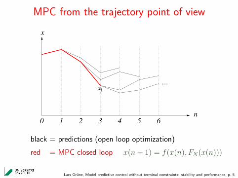
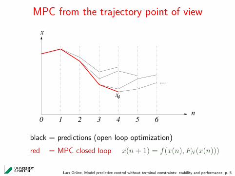
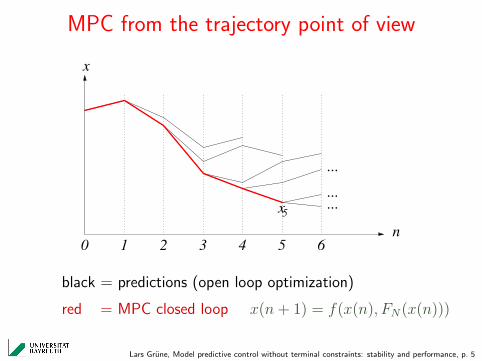
MPC from the trajectory point of view
0
n
x
0 1 2 3 4 5 6
x
black = predictions (open loop optimization)
red = MPC closed loop x(n+ 1) = f(x(n), FN(x(n)))
Lars Grune, Model predictive control without terminal constraints: stability and performance, p. 5
MPC from the trajectory point of view
0
n
x
0 1 2 3 4 5 6
x
black = predictions (open loop optimization)
red = MPC closed loop x(n+ 1) = f(x(n), FN(x(n)))
Lars Grune, Model predictive control without terminal constraints: stability and performance, p. 5
MPC from the trajectory point of view
1
n
x
0 1 2 3 4 5 6
x
black = predictions (open loop optimization)
red = MPC closed loop x(n+ 1) = f(x(n), FN(x(n)))
Lars Grune, Model predictive control without terminal constraints: stability and performance, p. 5
MPC from the trajectory point of view
1
n
x
0 1 2 3 4 5 6
x
black = predictions (open loop optimization)
red = MPC closed loop x(n+ 1) = f(x(n), FN(x(n)))
Lars Grune, Model predictive control without terminal constraints: stability and performance, p. 5
MPC from the trajectory point of view
2
n
x
0 1 2 3 4 5 6
x
black = predictions (open loop optimization)
red = MPC closed loop x(n+ 1) = f(x(n), FN(x(n)))
Lars Grune, Model predictive control without terminal constraints: stability and performance, p. 5
MPC from the trajectory point of view
2
n
x
0 1 2 3 4 5 6
x
black = predictions (open loop optimization)
red = MPC closed loop x(n+ 1) = f(x(n), FN(x(n)))
Lars Grune, Model predictive control without terminal constraints: stability and performance, p. 5
MPC from the trajectory point of view
3
n
x
0 1 2 3 4 5 6
x
black = predictions (open loop optimization)
red = MPC closed loop x(n+ 1) = f(x(n), FN(x(n)))
Lars Grune, Model predictive control without terminal constraints: stability and performance, p. 5
MPC from the trajectory point of view
3
n
x
0 1 2 3 4 5 6
...x
black = predictions (open loop optimization)
red = MPC closed loop x(n+ 1) = f(x(n), FN(x(n)))
Lars Grune, Model predictive control without terminal constraints: stability and performance, p. 5
MPC from the trajectory point of view
4
n
x
0 1 2 3 4 5 6
...
x
black = predictions (open loop optimization)
red = MPC closed loop x(n+ 1) = f(x(n), FN(x(n)))
Lars Grune, Model predictive control without terminal constraints: stability and performance, p. 5
MPC from the trajectory point of view
4
n
x
0 1 2 3 4 5 6
...
...x
black = predictions (open loop optimization)
red = MPC closed loop x(n+ 1) = f(x(n), FN(x(n)))
Lars Grune, Model predictive control without terminal constraints: stability and performance, p. 5
MPC from the trajectory point of view
5
n
x
0 1 2 3 4 5 6
...
...
x
black = predictions (open loop optimization)
red = MPC closed loop x(n+ 1) = f(x(n), FN(x(n)))
Lars Grune, Model predictive control without terminal constraints: stability and performance, p. 5
MPC from the trajectory point of view
5
n
x
0 1 2 3 4 5 6
...
...
...x
black = predictions (open loop optimization)
red = MPC closed loop x(n+ 1) = f(x(n), FN(x(n)))
Lars Grune, Model predictive control without terminal constraints: stability and performance, p. 5
MPC from the trajectory point of view
6
n
x
0 1 2 3 4 5 6
...
...
...x
black = predictions (open loop optimization)
red = MPC closed loop x(n+ 1) = f(x(n), FN(x(n)))
Lars Grune, Model predictive control without terminal constraints: stability and performance, p. 5
MPC: QuestionsQuestions in this talk:
When does MPC stabilize the system?
How good is the MPC feedback law compared to theinfinite horizon optimal solution?
Part 1: stabilizing MPC — survey on recent results
Part 2: economic MPC — some very recent results
In stabilizing MPC, stability can be ensured by includingadditional “stabilizing” terminal constraints in the finitehorizon problem. Here we consider problems without suchstabilizing constraints.
Main motivation: even for small optimization horizons N wecan — in principle — obtain large feasible sets, i.e., sets ofinitial values for which the finite horizon problem is well defined
Lars Grune, Model predictive control without terminal constraints: stability and performance, p. 6
MPC: QuestionsQuestions in this talk:
When does MPC stabilize the system?
How good is the MPC feedback law compared to theinfinite horizon optimal solution?
Part 1: stabilizing MPC
— survey on recent results
Part 2: economic MPC
— some very recent results
In stabilizing MPC, stability can be ensured by includingadditional “stabilizing” terminal constraints in the finitehorizon problem. Here we consider problems without suchstabilizing constraints.
Main motivation: even for small optimization horizons N wecan — in principle — obtain large feasible sets, i.e., sets ofinitial values for which the finite horizon problem is well defined
Lars Grune, Model predictive control without terminal constraints: stability and performance, p. 6
MPC: QuestionsQuestions in this talk:
When does MPC stabilize the system?
How good is the MPC feedback law compared to theinfinite horizon optimal solution?
Part 1: stabilizing MPC — survey on recent results
Part 2: economic MPC — some very recent results
In stabilizing MPC, stability can be ensured by includingadditional “stabilizing” terminal constraints in the finitehorizon problem. Here we consider problems without suchstabilizing constraints.
Main motivation: even for small optimization horizons N wecan — in principle — obtain large feasible sets, i.e., sets ofinitial values for which the finite horizon problem is well defined
Lars Grune, Model predictive control without terminal constraints: stability and performance, p. 6
MPC: QuestionsQuestions in this talk:
When does MPC stabilize the system?
How good is the MPC feedback law compared to theinfinite horizon optimal solution?
Part 1: stabilizing MPC — survey on recent results
Part 2: economic MPC — some very recent results
In stabilizing MPC, stability can be ensured by includingadditional “stabilizing” terminal constraints in the finitehorizon problem. Here we consider problems without suchstabilizing constraints.
Main motivation: even for small optimization horizons N wecan — in principle — obtain large feasible sets, i.e., sets ofinitial values for which the finite horizon problem is well defined
Lars Grune, Model predictive control without terminal constraints: stability and performance, p. 6
Stability without stabilizing terminal constraintsWithout stabilizing constraints, stability is known to hold for“sufficiently large optimization horizon N” [Alamir/Bornard ’95,
For obtaining a quantitative estimate we need quantitativeinformation.
A suitable condition is “exponential controllability through ` ”:
there exist constants C > 0, σ ∈ (0, 1) such that for eachxu(0) ∈ X there is u(·) with xu(k) ∈ X, u(k) ∈ U and
`(xu(k), u(k)) ≤ Cσk`∗(xu(0))
with `∗(x) = minu∈U
`(x, u)
Lars Grune, Model predictive control without terminal constraints: stability and performance, p. 7
Stability without stabilizing terminal constraintsWithout stabilizing constraints, stability is known to hold for“sufficiently large optimization horizon N” [Alamir/Bornard ’95,
Rawlings ’11] consider MPC for the infinite horizon averagedperformance criterion
J∞(x, u) = lim supK→∞
1
K
K−1∑k=0
`(xu(k, x), u(k))
Here ` reflects an “economic” cost (like, e.g., energyconsumption) rather than penalizing the distance to somedesired equilibrium
Lars Grune, Model predictive control without terminal constraints: stability and performance, p. 17
Economic MPC with terminal constraintsTypical result: Let x∗ ∈ X be an equilibrium for some u∗ ∈ U,i.e., f(x∗, u∗) = x∗. Consider an MPC scheme where in eachstep we minimize
JN(x, u) =1
N
N−1∑k=0
`(xu(k), u(k))
subject to the terminal constraint xu(N) = x∗.
Then for anyfeasible initial condition x ∈ X we get the inequality
J∞(x, FN) ≤ `(x∗, u∗)
Question: Does this also work without the terminal constraintxu(N) = x∗, i.e., is MPC able to find a good equilibrium x∗
“automatically”?
Lars Grune, Model predictive control without terminal constraints: stability and performance, p. 18
Economic MPC with terminal constraintsTypical result: Let x∗ ∈ X be an equilibrium for some u∗ ∈ U,i.e., f(x∗, u∗) = x∗. Consider an MPC scheme where in eachstep we minimize
JN(x, u) =1
N
N−1∑k=0
`(xu(k), u(k))
subject to the terminal constraint xu(N) = x∗. Then for anyfeasible initial condition x ∈ X we get the inequality
J∞(x, FN) ≤ `(x∗, u∗)
Question: Does this also work without the terminal constraintxu(N) = x∗, i.e., is MPC able to find a good equilibrium x∗
“automatically”?
Lars Grune, Model predictive control without terminal constraints: stability and performance, p. 18
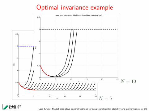
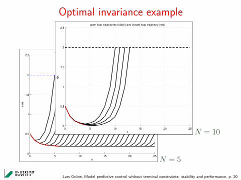
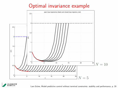
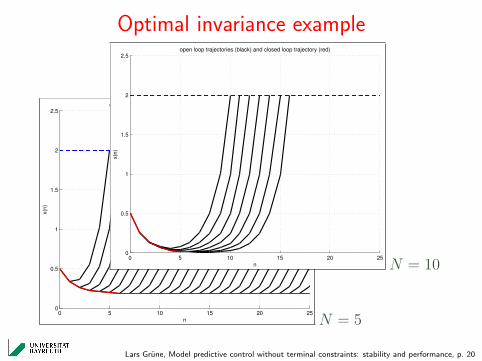
Economic MPC without terminal constraintsWe investigate this question for the following optimalinvariance problem:
Keep the state of the system inside an admissible set X withminimal infinite horizon averaged cost
J∞(x, u) = lim supK→∞
1
K
K−1∑k=0
`(xu(k, x), u(k))
Example: x(k + 1) = 2x(k) + u(k)
with X = [−2, 2], U = [−2, 2] and `(x, u) = u2
For this example, it is optimal to control the system to x∗ = 0and keep it there with u∗ = 0 inf
u∈U∞J∞(x, u) = 0
Lars Grune, Model predictive control without terminal constraints: stability and performance, p. 19
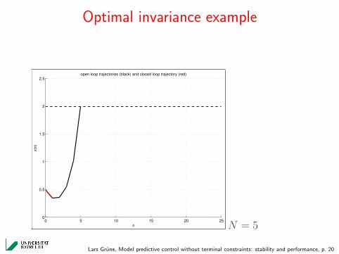
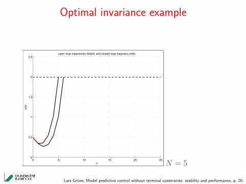
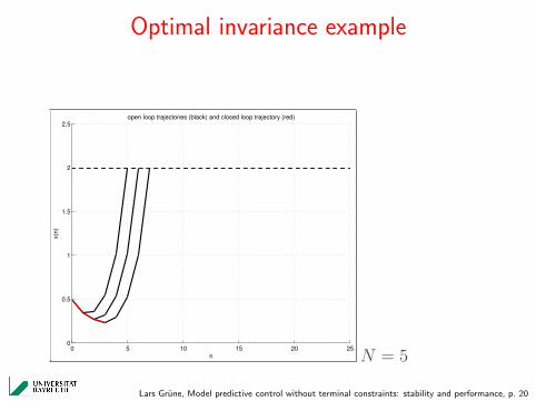
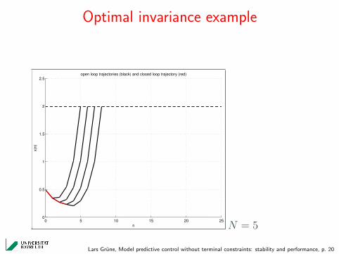
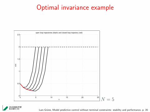
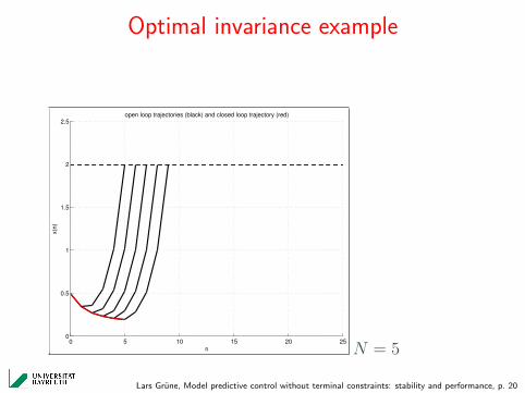
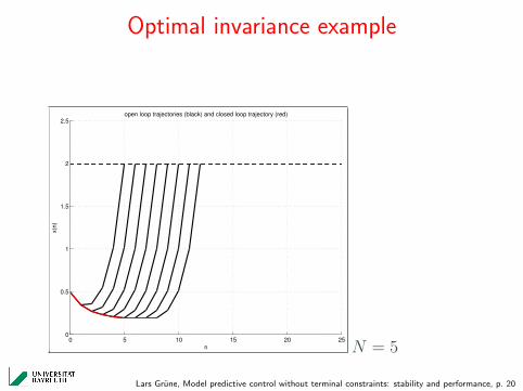
Optimal invariance example
0 5 10 15 20 250
0.5
1
1.5
2
2.5open loop trajectories (black) and closed loop trajectory (red)
n
x(n
)
N = 5
Lars Grune, Model predictive control without terminal constraints: stability and performance, p. 20
Optimal invariance example
0 5 10 15 20 250
0.5
1
1.5
2
2.5open loop trajectories (black) and closed loop trajectory (red)
n
x(n
)
N = 5
Lars Grune, Model predictive control without terminal constraints: stability and performance, p. 20
Optimal invariance example
0 5 10 15 20 250
0.5
1
1.5
2
2.5open loop trajectories (black) and closed loop trajectory (red)
n
x(n
)
N = 5
Lars Grune, Model predictive control without terminal constraints: stability and performance, p. 20
Optimal invariance example
0 5 10 15 20 250
0.5
1
1.5
2
2.5open loop trajectories (black) and closed loop trajectory (red)
n
x(n
)
N = 5
Lars Grune, Model predictive control without terminal constraints: stability and performance, p. 20
Optimal invariance example
0 5 10 15 20 250
0.5
1
1.5
2
2.5open loop trajectories (black) and closed loop trajectory (red)
n
x(n
)
N = 5
Lars Grune, Model predictive control without terminal constraints: stability and performance, p. 20
Optimal invariance example
0 5 10 15 20 250
0.5
1
1.5
2
2.5open loop trajectories (black) and closed loop trajectory (red)
n
x(n
)
N = 5
Lars Grune, Model predictive control without terminal constraints: stability and performance, p. 20
Optimal invariance example
0 5 10 15 20 250
0.5
1
1.5
2
2.5open loop trajectories (black) and closed loop trajectory (red)
n
x(n
)
N = 5
Lars Grune, Model predictive control without terminal constraints: stability and performance, p. 20
Optimal invariance example
0 5 10 15 20 250
0.5
1
1.5
2
2.5open loop trajectories (black) and closed loop trajectory (red)
n
x(n
)
N = 5
Lars Grune, Model predictive control without terminal constraints: stability and performance, p. 20
Optimal invariance example
0 5 10 15 20 250
0.5
1
1.5
2
2.5open loop trajectories (black) and closed loop trajectory (red)
n
x(n
)
N = 5
Lars Grune, Model predictive control without terminal constraints: stability and performance, p. 20
Optimal invariance example
0 5 10 15 20 250
0.5
1
1.5
2
2.5open loop trajectories (black) and closed loop trajectory (red)
n
x(n
)
N = 5
Lars Grune, Model predictive control without terminal constraints: stability and performance, p. 20
Optimal invariance example
0 5 10 15 20 250
0.5
1
1.5
2
2.5open loop trajectories (black) and closed loop trajectory (red)
n
x(n
)
N = 5
Lars Grune, Model predictive control without terminal constraints: stability and performance, p. 20
Optimal invariance example
0 5 10 15 20 250
0.5
1
1.5
2
2.5open loop trajectories (black) and closed loop trajectory (red)
n
x(n
)
N = 5
Lars Grune, Model predictive control without terminal constraints: stability and performance, p. 20
Optimal invariance example
0 5 10 15 20 250
0.5
1
1.5
2
2.5open loop trajectories (black) and closed loop trajectory (red)
n
x(n
)
N = 5
Lars Grune, Model predictive control without terminal constraints: stability and performance, p. 20
Optimal invariance example
0 5 10 15 20 250
0.5
1
1.5
2
2.5open loop trajectories (black) and closed loop trajectory (red)
n
x(n
)
N = 5
Lars Grune, Model predictive control without terminal constraints: stability and performance, p. 20
Optimal invariance example
0 5 10 15 20 250
0.5
1
1.5
2
2.5open loop trajectories (black) and closed loop trajectory (red)
n
x(n
)
N = 5
Lars Grune, Model predictive control without terminal constraints: stability and performance, p. 20
Optimal invariance example
0 5 10 15 20 250
0.5
1
1.5
2
2.5open loop trajectories (black) and closed loop trajectory (red)
n
x(n
)
N = 5
Lars Grune, Model predictive control without terminal constraints: stability and performance, p. 20
Optimal invariance example
0 5 10 15 20 250
0.5
1
1.5
2
2.5open loop trajectories (black) and closed loop trajectory (red)
n
x(n
)
N = 5
Lars Grune, Model predictive control without terminal constraints: stability and performance, p. 20
Optimal invariance example
0 5 10 15 20 250
0.5
1
1.5
2
2.5open loop trajectories (black) and closed loop trajectory (red)
n
x(n
)
N = 5
Lars Grune, Model predictive control without terminal constraints: stability and performance, p. 20
Optimal invariance example
0 5 10 15 20 250
0.5
1
1.5
2
2.5open loop trajectories (black) and closed loop trajectory (red)
n
x(n
)
N = 5
Lars Grune, Model predictive control without terminal constraints: stability and performance, p. 20
Optimal invariance example
0 5 10 15 20 250
0.5
1
1.5
2
2.5open loop trajectories (black) and closed loop trajectory (red)
n
x(n
)
N = 5
Lars Grune, Model predictive control without terminal constraints: stability and performance, p. 20
Optimal invariance example
0 5 10 15 20 250
0.5
1
1.5
2
2.5open loop trajectories (black) and closed loop trajectory (red)
n
x(n
)
N = 5
0 5 10 15 20 250
0.5
1
1.5
2
2.5open loop trajectories (black) and closed loop trajectory (red)
n
x(n
)
N = 10
Lars Grune, Model predictive control without terminal constraints: stability and performance, p. 20
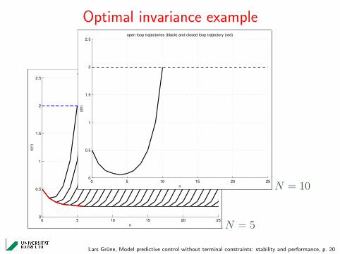
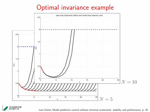
Optimal invariance: observations
0 5 10 15 20 250
0.5
1
1.5
2
2.5open loop trajectories (black) and closed loop trajectory (red)
n
x(n
)
N = 5 0 5 10 15 20 250
0.5
1
1.5
2
2.5open loop trajectories (black) and closed loop trajectory (red)
n
x(n
)
N = 10
optimal open loop trajectories first approach the optimalequilibrium and then tend to the boundary of X = [−2, 2]
closed loop trajectories follow the “good part” of theopen loop trajectories
the larger N , the “better” the closed loop trajectories.This is also reflected in the average closed loop costs
Lars Grune, Model predictive control without terminal constraints: stability and performance, p. 21
Optimal invariance: observations
0 5 10 15 20 250
0.5
1
1.5
2
2.5open loop trajectories (black) and closed loop trajectory (red)
n
x(n
)
N = 5 0 5 10 15 20 250
0.5
1
1.5
2
2.5open loop trajectories (black) and closed loop trajectory (red)
n
x(n
)
N = 10
optimal open loop trajectories first approach the optimalequilibrium and then tend to the boundary of X = [−2, 2]
closed loop trajectories follow the “good part” of theopen loop trajectories
the larger N , the “better” the closed loop trajectories.
This is also reflected in the average closed loop costs
Lars Grune, Model predictive control without terminal constraints: stability and performance, p. 21
Optimal invariance: observations
0 5 10 15 20 250
0.5
1
1.5
2
2.5open loop trajectories (black) and closed loop trajectory (red)
n
x(n
)
N = 5 0 5 10 15 20 250
0.5
1
1.5
2
2.5open loop trajectories (black) and closed loop trajectory (red)
n
x(n
)
N = 10
optimal open loop trajectories first approach the optimalequilibrium and then tend to the boundary of X = [−2, 2]
closed loop trajectories follow the “good part” of theopen loop trajectories
the larger N , the “better” the closed loop trajectories.This is also reflected in the average closed loop costs
Lars Grune, Model predictive control without terminal constraints: stability and performance, p. 21
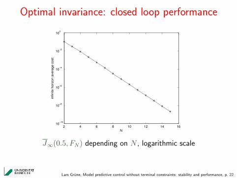
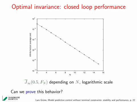
Optimal invariance: closed loop performance
2 4 6 8 10 12 14 1610
−10
10−8
10−6
10−4
10−2
100
N
infin
ite
ho
rizo
n a
ve
rag
e c
ost
J∞(0.5, FN) depending on N , logarithmic scale
Can we prove this behavior?
Lars Grune, Model predictive control without terminal constraints: stability and performance, p. 22
Optimal invariance resultTheorem [Gr. 11] Assume that there are N0 ≥ 0, `0 ∈ R andδ1, δ2 ∈ L such that for each x ∈ X and N ≥ N0 there existsa control sequence uN,x ∈ UN+1 satisfying
• xuN,x(k, x) ∈ X, k = 0, . . . , N + 1 admissibility
• JN(x, uN,x) ≤ infu∈U∞
JN(x, u) + δ1(N)/N near optimality
• `(xuN,x(N, x), uN,x(N)) ≤ `0 + δ2(N) small terminal value
Then J∞(x, FN(x)) ≤ `0 + δ1(N − 1) + δ2(N − 1) followsfor all x ∈ X.
These assumptions can be ensured by suitable controllabilityconditions plus bounds on the performance of certaintrajectories. For our invariance example, this allows torigorously prove J∞(x, FN)→ 0 as N →∞
Lars Grune, Model predictive control without terminal constraints: stability and performance, p. 23
Optimal invariance resultTheorem [Gr. 11] Assume that there are N0 ≥ 0, `0 ∈ R andδ1, δ2 ∈ L such that for each x ∈ X and N ≥ N0 there existsa control sequence uN,x ∈ UN+1 satisfying
• xuN,x(k, x) ∈ X, k = 0, . . . , N + 1 admissibility
• JN(x, uN,x) ≤ infu∈U∞
JN(x, u) + δ1(N)/N near optimality
• `(xuN,x(N, x), uN,x(N)) ≤ `0 + δ2(N) small terminal value
Then J∞(x, FN(x)) ≤ `0 + δ1(N − 1) + δ2(N − 1) followsfor all x ∈ X.
These assumptions can be ensured by suitable controllabilityconditions plus bounds on the performance of certaintrajectories.
For our invariance example, this allows torigorously prove J∞(x, FN)→ 0 as N →∞
Lars Grune, Model predictive control without terminal constraints: stability and performance, p. 23
Optimal invariance resultTheorem [Gr. 11] Assume that there are N0 ≥ 0, `0 ∈ R andδ1, δ2 ∈ L such that for each x ∈ X and N ≥ N0 there existsa control sequence uN,x ∈ UN+1 satisfying
• xuN,x(k, x) ∈ X, k = 0, . . . , N + 1 admissibility
• JN(x, uN,x) ≤ infu∈U∞
JN(x, u) + δ1(N)/N near optimality
• `(xuN,x(N, x), uN,x(N)) ≤ `0 + δ2(N) small terminal value
Then J∞(x, FN(x)) ≤ `0 + δ1(N − 1) + δ2(N − 1) followsfor all x ∈ X.
These assumptions can be ensured by suitable controllabilityconditions plus bounds on the performance of certaintrajectories. For our invariance example, this allows torigorously prove J∞(x, FN)→ 0 as N →∞
Lars Grune, Model predictive control without terminal constraints: stability and performance, p. 23
Summary and outlookMPC without terminal constraints shows excellent resultsboth for stabilizing and for economic problems
for stabilizing MPC, a controllability based analysis helpsto identify and design stage costs ` for obtaining stabilitywith small control horizons
for economic MPC, under suitable conditions an averageperformance close to that of an optimal equilibriumwithout a priori knowledge of this equilibrium can beachieved
Future work:
I extension of economic MPC results to more generalproblem classes and optimal periodic orbits
I (practical) asymptotic stability analysis of economicMPC without terminal constraints
Lars Grune, Model predictive control without terminal constraints: stability and performance, p. 24
Happy Birthday Eduardo!
Lars Grune, Model predictive control without terminal constraints: stability and performance, p. 25


![Concurrent Learning Adaptive Model Predictive Controlwith constraints is model predictive control (see e.g. [4, 30, 20]). While this tech-nique has been heavily studied and implemented](https://static.documents.pub/doc/80x56/5f088c4d7e708231d4228e15/concurrent-learning-adaptive-model-predictive-control-with-constraints-is-model.jpg)


