Modeling and Control of a Quadrotor UAV with Tilting Propellers

Markus Ryll, Heinrich H. Bulthoff, and Paolo Robuffo Giordano

Abstract— Standard quadrotor UAVs possess a limited mo-bility because of their inherent underactuation, i.e., availabilityof 4 independent control inputs (the 4 propeller spinningvelocities) vs. the 6 dofs parameterizing the quadrotor posi-tion/orientation in space. As a consequence, the quadrotor posecannot track an arbitrary trajectory over time (e.g., it can hoveron the spot only when horizontal). In this paper, we propose anovel actuation concept in which the quadrotor propellers areallowed to tilt about their axes w.r.t. the main quadrotor body.This introduces an additional set of 4 control inputs whichprovides full actuation to the quadrotor position/orientation.After deriving the dynamical model of the proposed quadrotor,we formally discuss its controllability properties and propose anonlinear trajectory tracking controller based on dynamic feed-back linearization techniques. The soundness of our approachis validated by means of simulation results.

I. INTRODUCTION

Unmanned aerial vehicles (UAVs) are a popular researchfield as attested by the increasing attention received over thelast years, see, e.g., [1], [2], [3], [4], [5]. The possibilityof using UAVs in various tasks such as data collection,search and rescue missions, or exploration and surveillanceof unaccessible disaster areas are fascinating both from ascientific viewpoint and from the potential beneficial impacton our society. Recent advances in this field have also beenpossible thanks to the progress, over the last decade, inmicroelectromechanical systems and sensors (MEMS) and inthe computational power of microcontrollers, which allowedto realize new micro UAVs with affordable costs.

While the small size of such UAVs is especially suit-able for surveillance tasks and/or indoor navigation, severalgroups are also starting to address the interesting possibilityto allow for an actual interaction with the environment, eitherin the form of direct contact [6], [7] or by consideringsimple grasping/manipulation tasks [8], [9]. This researchis motivated by the need of transitioning from the classicaltopic of “autonomous flying vehicles” into the more robotic-oriented “autonomous flying service robots”, that is flyingrobots able to accomplish typical manipulation tasks [10].However, major advancements in the complexity of the tasksenvisioned for future UAVs should also be followed byinnovative breakthroughs on the mechanical and actuationsides. In this respect, several possibilities have been proposedin the past literature spanning different concepts: ducted-fan

M. Ryll and P. Robuffo Giordano are with the Max Planck Institutefor Biological Cybernetics, Spemannstraße 38, 72076 Tubingen, Germany{markus.ryll,prg}@tuebingen.mpg.de.

H. H. Bulthoff is with the Max Planck Institute for Biological Cy-bernetics, Spemannstraße 38, 72076 Tubingen, Germany, and with theDepartment of Brain and Cognitive Engineering, Korea University, Anam-dong, Seongbuk-gu, Seoul, 136-713 Korea hhb@tuebingen.mpg.de.

designs [11], tilt-wing mechanisms [12], [13], or tilt-rotoractuations [14], [15].

Taking inspiration from these latter works, in this paperwe propose a novel actuation concept for a quadrotor UAVin which the (usually fixed) propellers are allowed to tiltabout the axes connecting them to the main body frame,thus realizing a ‘quad(tilt-)rotor UAV’. Indeed, one of thelimitations of the classical quadrotor design lies in its inher-ent underactuation: presence of only 4 independent controlinputs (the 4 propeller spinning velocities) does not allowto independently control the position and orientation of thequadrotor at the same time. For instance, in quasi-hoverconditions, an horizontal translation necessarily implies achange in the attitude or, symmetrically, a quadrotor canhover in place only when being horizontal w.r.t. the groundplane. On the other hand, in this paper we will show thatby means of these additional 4 actuated dofs it is possibleto gain full controllability over the quadrotor position andorientation, thus rendering it, as a matter of fact, a fullyactuated flying rigid body. Apart from the novel challengesthat this design represents from a control point of view, webelieve that endowing UAVs with full 6 dofs mobility willrepresent an important feature in many future applications,especially those involving interaction/manipulation in clut-tered environments where precise force/motion control willbe a mandatory need.

Goals of this paper are then: (i) to derive the dynamicalmodel of the proposed quadrotor with tilting propellers(Sect. II), (ii) to formally analyze its controllability prop-erties and to devise a closed-loop controller able to asymp-totically track an arbitrary desired trajectory for the quadrotorposition/orientation in space (Sect. III), and (iii) to presentsimulation results assessing the effectiveness and robustnessof this control strategy. Finally, Sect. V will conclude thepaper and discuss future perspectives.

II. QUADROTOR DYNAMIC MODEL

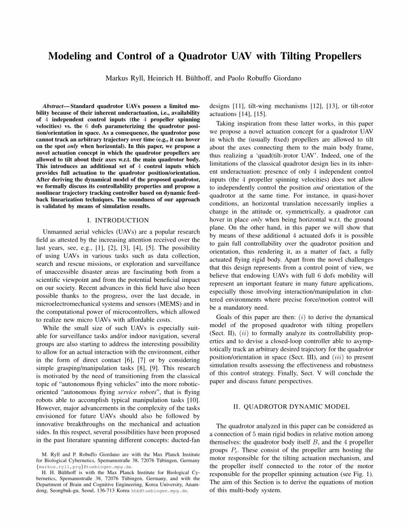
The quadrotor analyzed in this paper can be considered asa connection of 5 main rigid bodies in relative motion amongthemselves: the quadrotor body itself B, and the 4 propellergroups Pi. These consist of the propeller arm hosting themotor responsible for the tilting actuation mechanism, andthe propeller itself connected to the rotor of the motorresponsible for the propeller spinning actuation (see Fig. 1).The aim of this Section is to derive the equations of motionof this multi-body system.

Fig. 1: CAD model of the quadrotor with tilting propellers. Themodel is based on a quadrotor from mikrokopter.de, and is com-posed of: (1) Micro controller, (2) Brushless controller, (3) Lander,(4) Propeller motor, (5) Tilting actuator, (6) Battery.

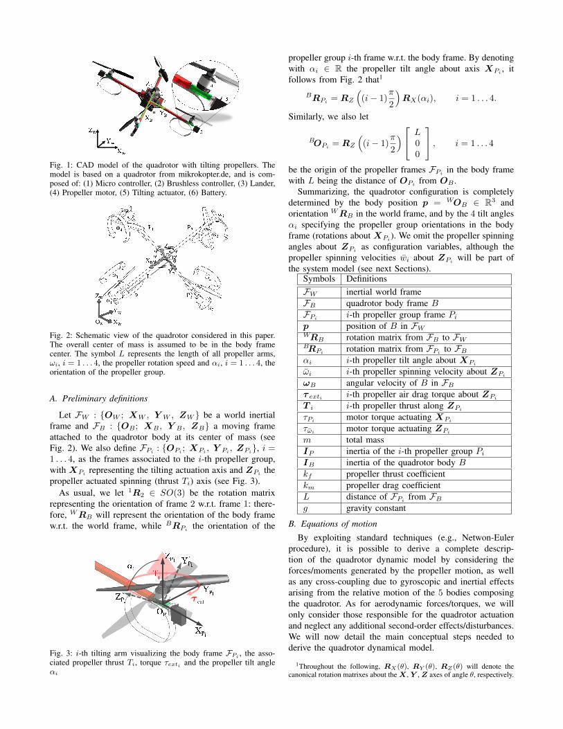
Fig. 2: Schematic view of the quadrotor considered in this paper.The overall center of mass is assumed to be in the body framecenter. The symbol L represents the length of all propeller arms,ωi, i = 1 . . . 4, the propeller rotation speed and αi, i = 1 . . . 4, theorientation of the propeller group.

A. Preliminary definitions

Let FW : {OW ; XW , Y W , ZW } be a world inertialframe and FB : {OB ; XB , Y B , ZB} a moving frameattached to the quadrotor body at its center of mass (seeFig. 2). We also define FPi

: {OPi; XPi

, Y Pi, ZPi

}, i =1 . . . 4, as the frames associated to the i-th propeller group,with XPi

representing the tilting actuation axis and ZPithe

propeller actuated spinning (thrust Ti) axis (see Fig. 3).As usual, we let 1R2 ∈ SO(3) be the rotation matrix

representing the orientation of frame 2 w.r.t. frame 1: there-fore, WRB will represent the orientation of the body framew.r.t. the world frame, while BRPi

the orientation of the

t

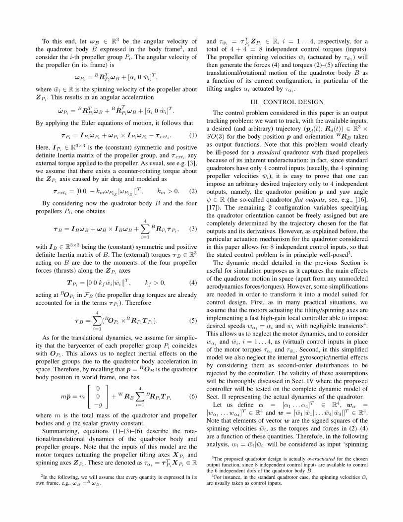
Fig. 3: i-th tilting arm visualizing the body frame FPi , the asso-ciated propeller thrust Ti, torque τexti and the propeller tilt angleαi

propeller group i-th frame w.r.t. the body frame. By denotingwith αi ∈ R the propeller tilt angle about axis XPi

, itfollows from Fig. 2 that1

BRPi= RZ

((i− 1)

π

2

)RX(αi), i = 1 . . . 4.

Similarly, we also let

BOPi= RZ

((i− 1)

π

2

) L00

, i = 1 . . . 4

be the origin of the propeller frames FPi in the body framewith L being the distance of OPi

from OB .Summarizing, the quadrotor configuration is completely

determined by the body position p = WOB ∈ R3 andorientation WRB in the world frame, and by the 4 tilt anglesαi specifying the propeller group orientations in the bodyframe (rotations about XPi

). We omit the propeller spinningangles about ZPi

as configuration variables, although thepropeller spinning velocities wi about ZPi will be part ofthe system model (see next Sections).

Symbols DefinitionsFW inertial world frameFB quadrotor body frame BFPi

i-th propeller group frame Pip position of B in FWWRB rotation matrix from FB to FWBRPi

rotation matrix from FPito FB

αi i-th propeller tilt angle about XPi

ωi i-th propeller spinning velocity about ZPi

ωB angular velocity of B in FBτ exti i-th propeller air drag torque about ZPi

T i i-th propeller thrust along ZPi

τPimotor torque actuating XPi

τωi motor torque actuating ZPi

m total massIP inertia of the i-th propeller group PiIB inertia of the quadrotor body Bkf propeller thrust coefficientkm propeller drag coefficientL distance of FPi from FBg gravity constant

B. Equations of motion

By exploiting standard techniques (e.g., Netwon-Eulerprocedure), it is possible to derive a complete descrip-tion of the quadrotor dynamic model by considering theforces/moments generated by the propeller motion, as wellas any cross-coupling due to gyroscopic and inertial effectsarising from the relative motion of the 5 bodies composingthe quadrotor. As for aerodynamic forces/torques, we willonly consider those responsible for the quadrotor actuationand neglect any additional second-order effects/disturbances.We will now detail the main conceptual steps needed toderive the quadrotor dynamical model.

1Throughout the following, RX(θ), RY (θ), RZ(θ) will denote thecanonical rotation matrixes about theX , Y ,Z axes of angle θ, respectively.

To this end, let ωB ∈ R3 be the angular velocity ofthe quadrotor body B expressed in the body frame2, andconsider the i-th propeller group Pi. The angular velocity ofthe propeller (in its frame) is

ωPi = BRTPiωB + [αi 0 wi]

T ,

where wi ∈ R is the spinning velocity of the propeller aboutZPi

. This results in an angular acceleration

ωPi= BRT

PiωB + BR

T

PiωB + [αi 0 ˙wi]

T .

By applying the Euler equations of motion, it follows that

τPi= IPi

ωPi+ ωPi

× IPiωPi− τ exti . (1)

Here, IPi∈ R3×3 is the (constant) symmetric and positive

definite Inertia matrix of the propeller group, and τ exti anyexternal torque applied to the propeller. As usual, see e.g. [3],we assume that there exists a counter-rotating torque aboutthe ZPi

axis caused by air drag and modeled as

τ exti = [0 0 − kmωPiZ|ωPiZ

|]T , km > 0. (2)

By considering now the quadrotor body B and the fourpropellers Pi, one obtains

τB = IBωB + ωB × IBωB +

4∑i=1

BRPiτPi

, (3)

with IB ∈ R3×3 being the (constant) symmetric and positivedefinite Inertia matrix of B. The (external) torques τB ∈ R3

acting on B are due to the moments of the four propellerforces (thrusts) along the ZPi

axes

T Pi= [0 0 kf wi|wi|]T , kf > 0, (4)

acting at BOPiin FB (the propeller drag torques are already

accounted for in the terms τPi ). Therefore

τB =

4∑i=1

(BOPi×BRPi

T Pi). (5)

As for the translational dynamics, we assume for simplic-ity that the barycenter of each propeller group Pi coincideswith OPi . This allows us to neglect inertial effects on thepropeller groups due to the quadrotor body acceleration inspace. Therefore, by recalling that p = WOB is the quadrotorbody position in world frame, one has

mp = m

00−g

+ WRB

4∑i=1

BRPiT Pi

(6)

where m is the total mass of the quadrotor and propellerbodies and g the scalar gravity constant.

Summarizing, equations (1)–(3)–(6) describe the rota-tional/translational dynamics of the quadrotor body andpropeller groups. Note that the inputs of this model are themotor torques actuating the propeller tilting axes XPi

andspinning axes ZPi

. These are denoted as ταi= τTPi

XPi∈ R

2In the following, we will assume that every quantity is expressed in itsown frame, e.g., ωB =BωB .

and τwi = τTPiZPi ∈ R, i = 1 . . . 4, respectively, for a

total of 4 + 4 = 8 independent control torques (inputs).The propeller spinning velocities wi (actuated by τwi

) willthen generate the forces (4) and torques (2)–(5) affecting thetranslational/rotational motion of the quadrotor body B asa function of its current configuration, in particular of thetilting angles αi actuated by ταi .

III. CONTROL DESIGN

The control problem considered in this paper is an outputtracking problem: we want to track, with the available inputs,a desired (and arbitrary) trajectory (pd(t), Rd(t)) ∈ R3 ×SO(3) for the body position p and orientation WRB takenas output functions. Note that this problem would clearlybe ill-posed for a standard quadrotor with fixed propellersbecause of its inherent underactuation: in fact, since standardquadrotors have only 4 control inputs (usually, the 4 spinningpropeller velocities wi), it is easy to prove that one canimpose an arbitrary desired trajectory only to 4 independentoutputs, namely, the quadrotor position p and yaw angleψ ∈ R (the so-called quadrotor flat outputs, see, e.g., [16],[17]). The remaining 2 configuration variables specifyingthe quadrotor orientation cannot be freely assigned but arecompletely determined by the trajectory chosen for the flatoutputs and its derivatives. However, as explained before, theparticular actuation mechanism for the quadrotor consideredin this paper allows for 8 independent control inputs, so thatthe stated control problem is in principle well-posed3.

The dynamic model detailed in the previous Section isuseful for simulation purposes as it captures the main effectsof the quadrotor motion in space (apart from any unmodeledaerodynamics forces/torques). However, some simplificationsare needed in order to transform it into a model suited forcontrol design. First, as in many practical situations, weassume that the motors actuating the tilting/spinning axes areimplementing a fast high-gain local controller able to imposedesired speeds wαi

= αi and wi with negligible transients4.This allows us to neglect the motor dynamics, and to considerwαi

and wi, i = 1 . . . 4, as (virtual) control inputs in placeof the motor torques ταi

and τwi. Second, in this simplified

model we also neglect the internal gyroscopic/inertial effectsby considering them as second-order disturbances to berejected by the controller. The validity of these assumptionswill be thoroughly discussed in Sect. IV where the proposedcontroller will be tested on the complete dynamic model ofSect. II representing the actual dynamics of the quadrotor.

Let us define α = [α1 . . . α4]T ∈ R4, wα =[wα1

. . . wα4]T ∈ R4 and w = [w1|w1| . . . w4|w4|]T ∈ R4.

Note that elements of vector w are the signed squares of thespinning velocities wi, as the torques and forces in (2)–(4)are a function of these quantities. Therefore, in the followinganalysis, wi = wi|wi| will be considered as input ‘spinning

3The proposed quadrotor design is actually overactuated for the chosenoutput function, since 8 independent control inputs are available to controlthe 6 independent dofs of the quadrotor body B.

4For instance, in the standard quadrotor case, the spinning velocities wiare usually taken as control inputs.

velocity’ of the i-th propeller, with the understanding that onecan always recover the actual speed wi = sign(wi)

√|wi|.

Under the stated assumptions, the quadrotor dynamicmodel can be simplified into

p =

00−g

+1

mWRBF (α)w

ωB = I−1B τ (α)w

α = wα

WRB = WRB [ωB ]∧

(7)

with [·]∧ being the usual map from R3 to so(3), and

F (α) =

0 −kfs2 0 kfs4−kfs1 0 kfs3 0kfc1 −kfc2 kfc3 −kfc4

,τ (α) =

0 −Lkf c2 − kms2 0−Lkf c1 + kms1 0 Lkf c3 − kms3−Lkfs1 − kmc1 Lkfs2 − kmc2 −Lkfs3 − kmc3Lkf c4 + kms4

0Lkfs4 − kmc4

(8)

the 3 × 4 input coupling matrixes (si = sin(αi) and ci =cos(αi)). Note that inputs w appear linearly in (7), asexpected. As in many output tracking problems, a conve-nient solution is to resort to output feedback linearizationtechniques (either static or dynamic), see [18] for a detailedtreatment. To this end, we rewrite the first two rows of (7)as

[p

ωB

]=

0

0−g

0

+

1

mWRB 0

0 I−1B

[F (α) 0

τ (α) 0

][w

wα

]

=f + JR[Jα(α) 0

] [ wwα

]= f + JRJα(α)

[w

wα

]

=f + J(α)

[w

wα

], (9)

where f ∈ R6 is a constant drift vector, J(α) ∈ R6×4,JR ∈ R6×6, and the 6×8 matrix J(α) will be referred to asthe output Jacobian. Assuming the map (9) is invertible, thatis ρJ = rank(J(α)) = 6, it is always possible to staticallyfeedback linearize (9) by means of the law[

w

wα

]= K(α)

(−f +

[pr

ωr

])(10)

where K(α) is a generalized inverse of J(α), e.g., thepseudoinverse J†(α), and [pTr ωTr ]T ∈ R6 an arbitraryreference linear/angular acceleration vector to be imposedto the output dynamics in (7).

However, this solution is not immediately viable in ourcase: in fact, ρJ = rank(J) = rank(JRJα) = rank(Jα)since JR is a nonsingular square matrix. Furthermore, ρJ =rank(Jα) = rank(Jα) ≤ 4 < 6 because of the structural

null matrix 0 ∈ R6×4 in matrix Jα(α) weighting the inputswα. Presence of this null matrix is due to the fact that inputswα affect the output dynamics at a higher differential levelcompared to inputs w. Therefore, a direct inversion at theacceleration level is bound to exploit only inputs w resultingin a loss of controllability for the system. Intuitively, theinstantaneous linear/angular acceleration of the quadrotorbody is directly affected by the propeller speedsw and tiltingconfiguration α (thanks to the dependance in Jα(α)), butnot by the tilting velocities α = wα. It is interesting to notethat this inhomogeneity in the differential levels at whichinputs are affecting the output dynamics is not a specificityof the system at hand. As an example, the same structuralproperty is also present in other robotic structures such asmobile manipulators with steering wheels [19] where the roleof wα is played by the wheel steering velocities.

A possible way to circumvent these difficulties and re-gain controllability is to exploit the null space of J (ofdimension ≥ 4) in order to optimize some ‘task feasibility’measure which, by acting on inputs wα, will orient the ρJ -dimensional range space of J(α) (ρJ ≤ 4) so as to spanthe desired 6-dimensional (task) vector (−f + [pTr ω

Tr ]T )

in (10). Alternatively, a somehow more systematic procedureis to resort to a dynamic output linearization scheme and seekto invert the input-output map at a higher differential levelwhere inputs wα will explicitly appear. Throughout the restof the Section we will focus on this latter approach.

By expanding the term Jα(α)w in (9) as

Jα(α)w =

4∑i=1

ji(α)wi,

and noting that

dJα(α)w

dt= Jα(α)w +

4∑i=1

∂ji(α)

∂αwαwi,

differentiation of (9) w.r.t. time yields[ ...p

ωB

]= JRJα(α)w + JR

4∑i=1

∂ji(α)

∂αwαwi + JRJα(α)w

= JR

[Jα(α)

∑4i=1

∂ji(α)

∂αwi

] [w

wα

]+ (11)[

WRBmF (α)w

0

]

= JRJ′α(α, w)

[w

wα

]+ b(α, w, ωB)

= A(α,w)

[w

wα

]+ b(α, w, ωB) (12)

where the new input w is the dynamic extension of theformer (and actual) input w obtained by adding 4 integratorson its channel5. Note that the new 6× 8 input-output decou-pling matrix A(α, w) is made of two column blocks: whilethe first block JRJα(α) is exactly the first block of the

5By means of this dynamic extensions, vector w becomes an internalstate of the controller.

former Jacobian J(α), the second block is not a null matrixas in the previous case. Rather, a new set of 4 columns,weighting inputs wα, are now present and contributing tothe rank of matrix A. It is particularly worth noting thatA(α, 0) = J(α): when the propellers are not spinning(w = 0), matrix A collapses back into the previous Jacobianmatrix J . Therefore, it will be mandatory for the controllerto ensure w 6= 0 at all times in order to keep the secondblock of A away from vanishing.

Assuming for now that matrix A has full row rank ρA =rank(A) = 6, it is then possible to invert (11) by means ofthe law[

w

wα

]= A†

([ ...pr

ωR

]− b)

+ (I8 −A†A)z, (13)

with IN being the identity matrix of dimension N , in orderto achieve full input-output linearization[ ...

p

ωB

]=

[ ...pr

ωR

]. (14)

The vector z ∈ R8 in (14) is an additional free quantityprojected onto the (2-dimensional) null space of A whoseuse will be detailed later on. We are now in position forsolving the control problem stated at the beginning of theSection, i.e., asymptotic tracking of a desired trajectory(pd(t), Rd(t)). Assuming pd(t) ∈ C3, it is sufficient to set...pr =

...pd+Kp1(pd−p)+Kp2(pd−p)+Kp3(pd−p) (15)

for obtaining exponential and decoupled convergence of theposition error to 0 as long as the (diagonal) positive definitegain matrixes Kp1 , Kp2 , Kp3 define Hurwitz polynomials.

As for the stabilization of the orientation tracking error,several choices are possible depending on the particular pa-rameterization chosen for the rotation matrix WRB . Besidesthe usual Euler angles (with their inherent singularity issues),an interesting possibility is to resort to an orientation errorterm directly defined on SO(3), as shown in [20], [17].Assume, as before, that Rd(t) ∈ C3 and let ωd = [RT

d Rd]∨,where [·]∨ represents the inverse map from so(3) to R3. Bydefining the orientation error as

eR =1

2[WRT

BRd −RTdWRB ]∨ (16)

the choice

ωr = ωd+Kω1(ωd−ωB)+Kω2

(ωd−ωB)+Kω3eR (17)

yields an exponential convergence for the orientation trackingerror to 0 as desired, provided that the (diagonal) gainmatrixes Kω1

, Kω2, Kω3

define a Hurwitz polynomial.Note that, although the body linear/angular accelerations

p and ωB appear as feedback terms in (15)–(17), a di-rect, and possibly noisy, acceleration measurement is notstrictly needed. In fact, these quantities can also be evaluatedin terms of sole velocity measurements (vector w) since,from (9), it follows that[

p

ωB

]= f + JRJα(α)w.

0 100 200 300 400 500 600 7000

50

100

150

200

250

300

350

400

450

500

hi(w

i)

|wi| [rad/s]

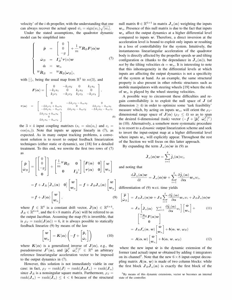
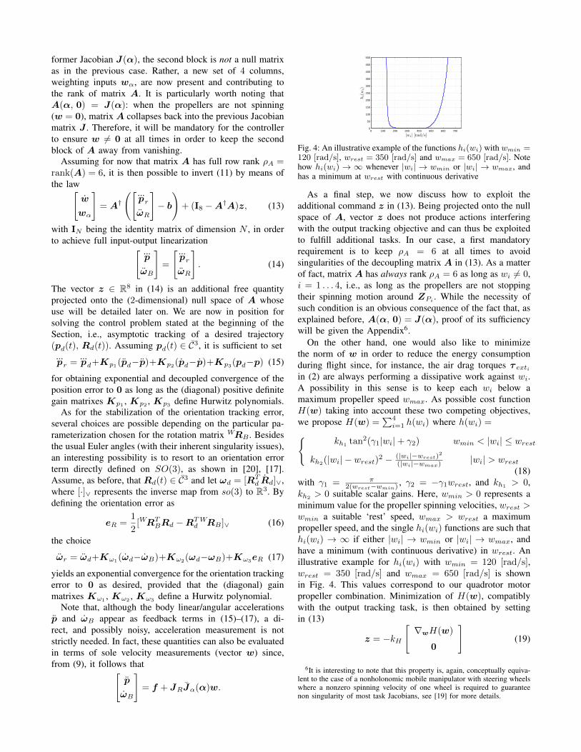
Fig. 4: An illustrative example of the functions hi(wi) with wmin =120 [rad/s], wrest = 350 [rad/s] and wmax = 650 [rad/s]. Notehow hi(wi) → ∞ whenever |wi| → wmin or |wi| → wmax, andhas a minimum at wrest with continuous derivative

As a final step, we now discuss how to exploit theadditional command z in (13). Being projected onto the nullspace of A, vector z does not produce actions interferingwith the output tracking objective and can thus be exploitedto fulfill additional tasks. In our case, a first mandatoryrequirement is to keep ρA = 6 at all times to avoidsingularities of the decoupling matrix A in (13). As a matterof fact, matrix A has always rank ρA = 6 as long as wi 6= 0,i = 1 . . . 4, i.e., as long as the propellers are not stoppingtheir spinning motion around ZPi

. While the necessity ofsuch condition is an obvious consequence of the fact that, asexplained before, A(α, 0) = J(α), proof of its sufficiencywill be given the Appendix6.

On the other hand, one would also like to minimizethe norm of w in order to reduce the energy consumptionduring flight since, for instance, the air drag torques τ extiin (2) are always performing a dissipative work against wi.A possibility in this sense is to keep each wi below amaximum propeller speed wmax. As possible cost functionH(w) taking into account these two competing objectives,we propose H(w) =

∑4i=1 h(wi) where h(wi) ={

kh1tan2(γ1|wi|+ γ2) wmin < |wi| ≤ wrest

kh2(|wi| − wrest)2 − (|wi|−wrest)

2

(|wi|−wmax) |wi| > wrest(18)

with γ1 = π2(wrest−wmin) , γ2 = −γ1wrest, and kh1

> 0,kh2

> 0 suitable scalar gains. Here, wmin > 0 represents aminimum value for the propeller spinning velocities, wrest >wmin a suitable ‘rest’ speed, wmax > wrest a maximumpropeller speed, and the single hi(wi) functions are such thathi(wi) → ∞ if either |wi| → wmin or |wi| → wmax, andhave a minimum (with continuous derivative) in wrest. Anillustrative example for hi(wi) with wmin = 120 [rad/s],wrest = 350 [rad/s] and wmax = 650 [rad/s] is shownin Fig. 4. This values correspond to our quadrotor motorpropeller combination. Minimization of H(w), compatiblywith the output tracking task, is then obtained by settingin (13)

z = −kH[∇wH(w)

0

](19)

6It is interesting to note that this property is, again, conceptually equiva-lent to the case of a nonholonomic mobile manipulator with steering wheelswhere a nonzero spinning velocity of one wheel is required to guaranteenon singularity of most task Jacobians, see [19] for more details.

0 5 10 150

0.5

1

1.5

2

2.5

3

θ(t)

[rad]

time [s]

Fig. 5: Profile of θ(t) for the first simulation

with kH > 0 being a suitable stepsize. Note that, as abyproduct, this choice will also result in a beneficial ‘velocitydamping’-like action on the states w as, e.g., describedin [21].

IV. SIMULATIONS

In the following, we will present two simulations per-formed by applying the controller presented in the previousSection on the dynamic model described in Sect. II. The aimis twofold: on one side, we want to highlight the trackingcapabilities of the proposed controller and the beneficialaction of the null-space term (19) in avoiding singularitiesfor matrix A. On the other side, we also want to test therobustness of the controller against all the inertial/gyroscopiceffects neglected at the control design stage but included inthe quadrotor dynamic model (1)–(3)–(6).

A. First simulation

In this first simulation, we tested a simple trajectoryinvolving a rotation of 0.94π [rad] on the spot along theXB

axis (this motion would be clearly unfeasible for a standardquadrotor). The initial conditions were set to p(t0) = 0,p(t0) = 0, WRB(t0) = I3, ωB(t0) = 0, α(t0) = 0,α(t0) = 0, and w(t0) = wrest. The desired trajectory waschosen as pd(t) ≡ 0 and Rd(t) = RX(θ(t)) with θ(t)following the smooth profile shown in Fig. 5 with maximumvelocity θmax = 1 [rad/s] and maximum accelerationθmax = 0.5 [rad/s2]. The trajectory was executed twiceby (i) including and (ii) not including the null-space termz (19) into (13) (kH = 1 or kH = 0). The gains in (15)–(17)were set to Kp1 = Kω1

= 7.5 I3, Kp2 = Kω2= 18.75 I3,

Kp3 = Kω3= 15.62 I3, and kh1

= 1, kh2= 10 in (18).

Figures 6(a–f) show the results of the simulation in thesetwo cases. In particular, Fig. 6(a) shows the superimpositionof H(w) when including z (red dashed line, case (i)) and notincluding z (blue solid line, case (ii)). It is clear that, in thelatter case, H(w) attains a lower value over time thanks tothe optimization action in (19). As a consequence, this resultsin a lower value for ‖w‖ over time as depicted in Fig. 6(b)(same color pattern), showing that the given task (rotationon the spot) can be realized in a more ‘energy-efficient’way when properly shaping the cost function H(w). Notethat, as a byproduct, the better performance of case (i)comes at the expense of a more complex reorientation ofthe propeller groups during the motion. This is shown inFigs. 6(c–d) which report the behavior of the 4 tilt angles

0 5 10 150

0.5

1

1.5

2

2.5

3

3.5

4

4.5

5x 10

7

H(w

)

time [s]

(a)

0 5 10 15800

850

900

950

1000

1050

1100

‖w‖[rad/s2]

time [s]

(b)

0 5 10 15−200

−150

−100

−50

0

50

100

150

200

α[rad]

time [s]

(c)

0 5 10 15−200

−150

−100

−50

0

50

100

150

200

α[rad]

time [s]

(d)

0 5 10 15−0.025

−0.02

−0.015

−0.01

−0.005

0

0.005

0.01

0.015

0.02

e p[m

]

time [s]

(e)

0 5 10 15−0.4

−0.3

−0.2

−0.1

0

0.1

0.2

0.3

e R[rad]

time [s]

(f)

Fig. 6: Results of the first simulation with (i) and without (ii)exploiting the null-space term (19). 6(a): behavior of H(w) forcases (i) (red dashed line) and (ii) (blue solid line). 6(b): behaviorof ‖w‖ for cases (i) (red dashed line) and (ii) (blue solid line).6(c–d): behavior of the tilt angles α for cases (i) (left) and (ii)(right). 6(e–f): behavior of the position/orientation tracking errors(ep, eR) for case (ii).

αi in cases (i) (left) and (ii) (right): compared to Fig. 6(d),note the rotation of two propellers starting from t ≈ 4 [s]in Fig. 6(c). Finally, Figs. 6(e–f) show the position trackingerror ep(t) = pd(t) − p(t) and orientation tracking erroreR(t) (16) only for case (i). Despite the fast reorientationof two propellers highlighted in Fig. 6(d), the tracking errorsstay small (note the scales) and eventually converge to zeroas the desired trajectory comes to a full stop. This providesa first confirmation of the validity of our assumptions inSect. III, that is, robustness of the controller w.r.t. any gy-roscopic/inertial effect due to the internal relative motion ofthe different bodies composing the quadrotor. This point willalso be addressed more thoroughly by the next simulation.

For the reader’s convenience, we also report in Figs. 7(a–b) a series of snapshots illustrating the quadrotor motion inthese two cases.

B. Second simulation

In the second simulation, we addressed the case of a morecomplex trajectory following a square path with vertexes{V1, V2, V3, V4, V5}. Each vertex was associated with the

(a) (b)Fig. 7: Results of the first simulation. Left column: quadrotormotion during case (i). Right column: quadrotor motion duringcase (ii). Note the large reorientation of the propeller groups inthis latter case thanks to the action of the optimization term (19)

following desired positions and orientations7

• V 1: pd = [0 0 0]T , ηd = [0 0 0]T

• V 2: pd = [0 3 1]T , ηd = [0 − π/2 0]T

• V 3: pd = [2 3 1]T , ηd = [−π/4 0 − π/4]T

• V 4: pd = [2 0 0]T , ηd = [−1.41 − 1.08 0.25]T

• V 5: pd = [0 0 0]T , ηd = [0.31 − 1.08 0.25]T

which were traveled along with rest-to-rest motions withmaximum linear/angular velocities of 1 [m/s] and 1 [rad/s],and maximum linear/angular accelerations of 1 [m/s2] and0.2 [rad/s2]. Figure 8 shows a series of snapshots illus-trating the overall motion, while Figs. 9(a–d) show thedesired trajectory (pd(t), ηd(t)), and the tracking errors(ep(t), eR(t)). Note again how the tracking errors keeplimited as before despite the more complex motion involv-ing several reorientations of the propellers. This confirmsagain the validity of the controller proposed in the previousSection. The interested reader can also refer to the videoattached to the paper for a more exhaustive illustration ofthe quadrotor motion capabilities.

V. CONCLUSIONS AND FUTURE WORKS

In this paper, we have addressed the modeling and controlissues for a quadrotor UAV with a novel actuation conceptwhich allows the 4 propellers to actively rotate (tilt) aboutthe axes connecting them to the quadrotor main body. The

7Here, for the sake of clarity, we represent orientations by means of theclassical roll/pitch/yaw Euler set η ∈ R3.

Fig. 8: Trajectory (red line) with SQC visualized in accordingorientations during the maneuver

0 2 4 6 8 10 12 14 16 180

0.5

1

1.5

2

2.5

3

3.5

p d[m

]time [s]

(a)

0 2 4 6 8 10 12 14 16 18−90

−80

−70

−60

−50

−40

−30

−20

−10

0

10

η d[rad]

time [s]

(b)

0 2 4 6 8 10 12 14 16 18−0.08

−0.06

−0.04

−0.02

0

0.02

0.04

0.06

0.08

e p[m

]

time [s]

(c)

0 2 4 6 8 10 12 14 16 18−0.08

−0.06

−0.04

−0.02

0

0.02

0.04

0.06

0.08

0.1

e R[rad

]

time [s]

(d)

Fig. 9: Fig. 9-a: Desired position pd in x, y and z; Fig. 9-b: Desiredorientation η in roll, pitch and yaw; Fig. 9-c: Position tracking errorep; Fig. 9-c: Orientation tracking error eR;

addition of this new set of 4 control inputs makes it possibleto (i) gain full controllability over the 6-dof quadrotorpose, and (ii) exploit the resulting actuation redundancy (oforder 2) so as to optimize suitable energy-efficiency criteria.After carefully analyzing the controllability properties of thesystem, we proposed a trajectory tracking controller basedon dynamic feedback linearization techniques, and provideda validation by means of extensive simulations on a numberof reference trajectories.

Our next steps are aimed at, on one side, devising andcomparing additional control designs based on differenttechniques (e.g., backstepping, sliding mode), and, on theother side, at realizing a first prototype of the proposedquadrotor in order to work towards an actual implementationof the ideas discussed in this paper.

APPENDIXPropositon 1: If wi 6= 0, i = 1 . . . 4, then ρA =

rank(A) = 6.Proof: From (11), note that rank(A) =

rank(JRJ′α) = rank(J ′α) since JR is a square nonsingular

matrix. We now look for suitable nonsingular matrixesM ∈ R6×6 and N ∈ R8×8 such that MJ ′αN is in rowcanonical form, that is

MJ ′αN =[I6 ∗

]. (20)

If this manipulation is possible, then rank(A) =rank(J ′α) = rank(MJ ′αN) = 6. By inspection of J ′α,and after some (tedious) manipulations, a suitable M canbe found as

M =

M11 M12 M13 M14 M15 M16

M21 0 0 M24 0 0M31 M32 M33 M34 M35 M36

M41 M42 M43 M44 M45 M46

M51 0 0 M54 0 0M61 M62 M63 M64 M65 M66

with

M11 = −kmkfLs1 + (2k2m + k2fL

2)c1

2L2k3fw1

, M12 = −Lkf c1 − kms1

2Lk2fw1

,

M13 = −Lkfs1 + kmc1

2Lk2fw1

, M14 =Lkfs1 + 2kmc1

2L2k2fw1

,

M15 =s1

2Lkfw1

, M16 = −c1

2Lkfw1

,

M21 = −Lkf c2 + kms2

Lk2fw2

, M24 =s2

Lkfw2

,

M31 = −−Lkmkf c3 + (2k2m + L2k2f )s3

2L2k3f, M32 =

Lkfs3 + kmc3

2Lk2f,

M33 =Lkf c3 − kms3

2Lk2f, M34 = −

Lkf c3 − 2kms3

2L2k2f,

M35 =c3

2Lkf, M36 = −

s3

2Lkf,

M41 = −−Lkmkf c1 + (2k2m + L2k2f )s1

2L2k3f, M42 = −

Lkfs1 + kmc1

2Lk2f,

M43 =Lkf c1 − kms1

2Lk2f, M44 = −

Lkf c1 − 2kms1

2L2k2f,

M45 = −c1

2Lkf, M46 = −

s1

2Lkf,

M51 = −Lkfs2 − kmc2

Lk2f, M54 = −

c2

Lkf,

M61 = −Lkfkms3 + (2k2m + L2k2f )c3

2L2k3fw3

, M62 =Lkf c3 − kms3

2Lk2fw3

,

M63 = −Lkfs3 + kmc3

2Lk2fw3

, M64 =Lkfs3 + 2kmc3

2L2k2fw3

,

M65 = −s3

2Lkfw3

, M66 = −c1

2Lk2fw3

,

and det(M) = − 1

4L3k6fw1w2w3

. As for N , it is just a

column permutation matrix

N =

1 0 0 0 0 0 0 00 1 0 0 0 0 0 00 0 1 0 0 0 0 00 0 0 0 0 0 1 00 0 0 1 0 0 0 00 0 0 0 1 0 0 00 0 0 0 0 1 0 00 0 0 0 0 0 0 1

.

It is then easy to see that, if w1 6= 0, w2 6= 0 and w3 6= 0,matrix M is always well-defined and (20) always holds,proving that ρA = rank(A) = 6. Note that in this case,because of the particular choice made for M , no conditionis present on w4 (w4 could vanish). This is coherent withthe intuition that three actuated propellers can be sufficientto provide full mobility to the quadrotor body (6 inputs for6 rigid body dofs). However, presence of a fourth activepropeller (w4 6= 0 in this case) guarantees the neededactuation redundancy exploited in Sect. III.

ACKNOWLEDGEMENTS

This research was partly supported by WCU (World ClassUniversity) program funded by the Ministry of Education,Science and Technology through the National ResearchFoundation of Korea (R31-10008).

REFERENCES

[1] D. Gurdan, J. STumpf, M. Achtelik, K.-M. Dorh, G. Hirzinger,and D. Rus, “Energy-efficient autonomous four-rotor flying robotcontrolled at 1 kHz,” in 2007 IEEE Int. Conf. on Robotics andAutomation, 2007, pp. 361–366.

[2] S. Bouabdallah, M. Becker, and R. Siegwart, “Autonomous miniatureflying robots: Coming soon!” IEEE Robotics and Automation Maga-zine, vol. 13, no. 3, pp. 88–98, 2007.

[3] K. P. Valavanis, Ed., Advances in Unmanned Aerial Vehicles: State ofthe Art and the Road to Autonomy. Springer, 2007.

[4] D. Mellinger, N. Michael, and V. Kumar, “Trajectory generation andcontrol for precise aggressive maneuvers with quadrotors,” in Proc. ofthe 2010 Int. Symposium on Experimental Robotics, 2010.

[5] P. Pounds, R. Mahony, and P. Corke, “Modelling and control of alarge quadrotor robot,” Control Engineering Practice, vol. 18, no. 7,pp. 691–699, 2010.

[6] L. Gentili, R. Naldi, and L. Marconi, “Modelling and control ofVTOL UAVs interacting with the environment,” in 2008 IEEE Conf.on Decision and Control, 2008, pp. 1231–1236.

[7] R. Naldi and L. Marconi, “Modeling and control of the interactionbetween flying robots and the environment,” in Proc. of the 2010 IFACNOLCOS, 2010.

[8] P. E. I. Pound, D. R. Bersak, and A. M. Dollar, “Grasping from theair: Hovering capture and load stability,” in 2011 IEEE Int. Conf. onRobotics and Automation, 2011, pp. 2491–2498.

[9] Q. Lindsey, D. Mellinger, and V. Kumar, “Construction of cubicstructures with quadrotor teams,” in Robotics: Science and Systems,2011.

[10] EU Collaborative Project ICT-248669 AIRobots, “www.airobots.eu.”[11] R. Naldi, L. Gentili, L. Marconi, and A. Sala, “Design and experi-

mental validation of a nonlinear control law for a ducted-fan miniatureaerial vehicle,” Control Engineering Practice, vol. 18, no. 7, pp. 747–760, 2010.

[12] K. T. Oner, E. Cetinsoy, M. Unel, M. F. Aksit, I. Kandemir, andK. Gulez, “Dynamic model and control of a new quadrotor unmannedaerial vehicle with tilt-wing mechanism,” in Proc. of the 2008 WorldAcademy of Science, Engineering and Technology, 2008, pp. 58–63.

[13] K. T. Oner, E. Cetinsoy, E. Sirimoglu, C. Hancer, T. Ayken, andM. Unel, “LQR and SMC stabilization of a new unmanned aerialvehicle,” in Proc. of the 2009 World Academy of Science, Engineeringand Technology, 2009, pp. 554–559.

[14] F. Kendoul, I. Fantoni, and R. Lozano, “Modeling and control of asmall autonomous aircraft having two tilting rotors,” IEEE Trans. onRobotics, vol. 22, no. 6, pp. 1297–1302, 2006.

[15] A. Sanchez, J. Escareno, O. Garcia, and R. Lozano, “Autonomoushovering of a noncyclic tiltrotor UAV: Modeling, control and imple-mentation,” in Proc. of the 17th IFAC Wold Congress, 2008, pp. 803–808.

[16] V. Mistler, A. Benallegue, and N. K. M’Sirdi, “Exact linearization andnoninteracting control of a 4 rotors helicopter via dynamic feedback,”in Proc. of the 10th IEEE International Workshop on Robot andHuman Interactive Communication, 2001, pp. 586–593.

[17] D. Mellinger and V. Kumar, “Minimum snap trajectory generationand control for quadrotors,” in 2011 IEEE Int. Conf. on Robotics andAutomation, 2011, pp. 2520–2525.

[18] A. Isidori, Nonlinear Control Systems, 3rd ed. Springer, 1995.[19] A. De Luca, G. Oriolo, and P. Robuffo Giordano, “Kinematic control

of nonholonomic mobile manipulators in the presence of steeringwheels,” in 2010 IEEE Int. Conf. on Robotics and Automation, 2010,pp. 1792–1798.

[20] T. Lee, M. Leok, and N. H. McClamroch, “Geometric tracking controlof a quadrotor UAV on SE(3),” in 2010 IEEE Conf. on Decision andControl, 2010, pp. 5420–5425.

[21] A. De Luca, G. Oriolo, and B. Siciliano, “Robot redundancy resolutionat the acceleration level,” Robotica, vol. 4, no. 2, pp. 97–106, 1992.