ALMA MATER STUDIORUM - UNIVERSIT ` A DI BOLOGNA SEDE DI CESENA SECONDA FACOLT ` A DI INGEGNERIA CON SEDE A CESENA CORSO DI LAUREA MAGISTRALE IN INGEGNERIA BIOMEDICA TITOLO DELLA TESI MODELING AND SIMULATION OF A SYNTHETIC GENETIC CIRCUIT THAT IMPLEMENTS A MULTICELLED BEHAVIOR IN A GROWING MICROCOLONY OF E. COLI Tesi in: Bioingegneria Molecolare e Cellulare LM Relatore Prof. Ing. Stefano Severi Correlatori Presentata da Prof. Emanuele Domenico Giordano Andrea Samor´ e Ing. Seunghee Shelly Jang Prof. Ing. Eric Klavins Sessione III Anno Accademico 2011/2012
Transcript
ALMA MATER STUDIORUM - UNIVERSITA DI BOLOGNASEDE DI CESENA
SECONDA FACOLTA DI INGEGNERIA CON SEDE A CESENACORSO DI LAUREA MAGISTRALE IN INGEGNERIA
3.1.1 Promoter regulated by a repressor . . . . . . . . . . . . 313.1.2 Promoter regulated by an activator . . . . . . . . . . . 333.1.3 Binding of an inducer to a transcription factor . . . . . 333.1.4 Hybrid promoter regulated by a repressor and an acti-
3.1 Input function of a gene regulated by a repressor with kd = 10 333.2 Input function of a gene regulated by an activator with kd = 10 343.3 Input function of an hybrid promoter with kdA = kdR = 10
4.1 Simulation of stochastic production and degradation of redfluorescent protein (RFP). The cells are genetically identicalbut the amount of protein differs slightly between individuals,note the different red intensity . . . . . . . . . . . . . . . . . . 44
4.2 Example of sensitivity plot. The parameter βLuxI is variedover about two orders of magnitude around its nominal value,depicted as a yellow square. . . . . . . . . . . . . . . . . . . . 48
4.3 Fitting of the cost function . . . . . . . . . . . . . . . . . . . . 484.4 Structure of the scatter plot used to rank the parameters. On
the left, the information that has been used to place the βLuxIdot in the right-hand graph. . . . . . . . . . . . . . . . . . . . 49
4.5 The four zones of the scatter plot used to rank the parameters 504.6 Scatter plots when the goal is set to a majority of followers. . 52
4
4.7 The goal is set to a majority of followers. Left-hand column:cost function of the four most promising parameters. Right-hand column: the corresponding fraction of leaders, followersand undecided cells are depicted in green, red and black. . . . 54
4.8 Scatter plot when the goal is to obtain a population in whichthere are about as many leaders as followers. . . . . . . . . . . 55
4.9 The goal is set to a colony split in half between leaders andfollowers. Left-hand column: cost function of the four mostpromising parameters. Right-hand column: the correspondingfraction of leaders, followers and undecided cells are depictedin green, red and black. . . . . . . . . . . . . . . . . . . . . . . 56
4.10 Scatter plot when the goal is set to a majority of leaders. . . . 584.11 The goal is set to a majority of leaders. Left-hand column:
cost function of the four most promising parameters. Right-hand column: the corresponding fraction of leaders, followersand undecided cells are depicted in green, red and black. . . . 59
4.12 Example of pattern created by a Ben-Jacob’s bacterial strain.The image of P. vortex colony was created at Prof. Ben-Jacob’s lab, at Tel-Aviv University, Israel . . . . . . . . . . . . 62
4.13 Simulation of the spots-forming finite state machine . . . . . . 654.14 Simulation of the rings-forming finite state machine . . . . . . 67
La Biologia Sintetica e una disciplina relativamente nuova, nata nei primianni duemila, che porta il tipico approccio ingegneristico al campo delle bio-tecnologie: astrazione, modularita e standardizzazione vengono utilizzati pertentare di domare l’estrema complessita dei componenti e costruire sistemibiologici artificiali con una funzione definita. Questi sistemi, tipicamente cir-cuiti genetici sintetici, vengono perlopiu implementati in batteri e sempliciorganismi eucariotici come ad esempio i lieviti. La cellula diventa quindiuna macchina programmabile ed il suo linguaggio macchina e costituito dasequenze nucleotidiche.
Il lavoro di tesi e stato svolto in collaborazione con ricercatori del De-partment of Electrical Engineering dell’Universita di Washington a Seattlee con una studentessa del Corso di Laurea in Ingegneria Biomedica dell’U-niversita di Bologna: Marilisa Cortesi. Nell’ambito della collaborazione hocontribuito ad un progetto di Biologia Sintetica gia avviato nel Klavins Lab,in particolare mi sono occupato della modellazione matematica e simulazionedi un circuito genetico sintetico pensato per implementare un comportamentomulticellulare in una microcolonia batterica.
Nel Primo Capitolo sono introdotte le basi della biologia molecolare, inparticolare si accenna alla struttura degli acidi nucleici e vengono illustrati iprocessi di trascrizione e traduzione che danno luogo all’espressione genica.Sono inoltre enunciati i principali meccanismi di regolazione dell’espressio-ne genica sia al livello trascrizionale che traduzionale. Un’introduzione allabiologia sintetica completa la sezione.
Nel Secondo capitolo e descritto il circuito genetico sintetico pensato perfar emergere spontaneamente due gruppi di cellule differenti, detti leaders efollowers, a partire da una colonia isogenica. Il circuito si basa sull’intrinsecastocasticita dell’espressione genica e sulla comunicazione intercellulare permezzo di una piccola molecola segnale per rompere la simmetria nel fenotipodella microcolonia. Sono illustrati inoltre i quattro moduli di cui il circuitosi compone (coin flipper, sender, receiver e follower) e le loro interazioni.
Nel Terzo Capitolo viene esposta la derivazione del modello matematico
6
dei singoli componenti del circuito genetico sintetico. Vengono poi esplici-tate le varie assunzioni semplificative che si sono rivelate necessarie al finedi ridurne la complessita e quindi permetterne la simulazione. Trascrizionee traduzione sono modellate in un unico passo e l’espressione dei vari genidipende dalla concentrazione intracellulare dei fattori di trascrizione che agi-scono sui promotori utilizzati. Sono infine elencati i valori dei vari parametrie le fonti da cui sono stati ricavati.
Nel Quarto Capitolo sono dapprima descritte le caratteristiche principa-li dell’ambiente di simulazione, gro, sviluppato dal Self Organizing SystemsLaboratory dell’Universita di Washington. Viene poi dettagliata l’analisi disensitivita svolta per individuare quali caratteristiche dei diversi componentigenetici sono desiderabili per il funzionamento del circuito. In particolare, edefinita una funzione costo basata sia sul numero di cellule che si trovano inognuno dei vari stati possibili al termine della simulazione che sul risultatovoluto. In base alla funzione costo e tramite un tipo particolare di scatterplot, viene stilata una classifica di parametri. A partire da una condizioneiniziale in cui i parametri assumono valori in un ordine di grandezza compa-tibile con le informazioni attualmente disponibili nella letteratura scientifica,questa classifica suggerisce quale componente genetico conviene regolare alfine di ottenere il risultato voluto. Il comportamento per cui il circuito estato ideato, ottenere una colonia in cui la quasi totalita di cellule siano nellostato follower e solo qualcuna nello stato leader, sembra essere il piu difficileda raggiungere. Poche cellule leader non riescono a produrre abbastanza se-gnale per far passare il resto della colonia nello stato follower. Per ottenereuna colonia in cui la maggioranza di cellule sia nello stato follower e necessa-rio aumentare il piu possible la produzione dell’enzima che genera il segnale.Ottenere una colonia in cui meta delle cellule sia nello stato leader e l’altrameta nello stato follower e piu semplice. La strategia piu promettente sem-bra essere aumentare leggermente la produzione di enzima. Per ottenere unamaggioranza di cellule leader, invece, e consigliabile aumentare l’espressionebasale dei geni nel modulo coin flipper. Al termine del capitolo, una possibileapplicazione futura del circuito genetico sintetico, la formazione spontaneadi pattern spaziali in una microcolonia, e modellata ad un alto livello diastrazione tramite il formalismo degli automi a stati finiti. La simulazionein gro fornisce indicazioni sui componenti genetici non ancora disponibili eche e quindi necessario sviluppare al fine di ottenere questo comportamento.In particolare, dato che entrambi gli esempi di pattern proposti si basanosu una versione locale di Leader Election, e essenziale utilizzare un metododi comunicazione intercellulare a corto raggio. Risulta inoltre fondamentalesviluppare componenti genetici che permettano di rallentare la crescita dispecifiche cellule senza alterarne la capacita di espressione genica.
7
L’Appendice, infine, contiene il codice utilizzato per simulare il modello ingro, il listato di uno script Python utile per parallelizzare l’analisi di sensi-tivita su un cluster Linux ed il codice Matlab con cui sono stati elaborati idati provenienti dall’analisi di sensitivita.
8
Abstract
Synthetic Biology is a relatively new discipline, born at the beginning ofthe New Millennium, that brings the typical engineering approach (abstrac-tion, modularity and standardization) to biotechnology. These principlesaim to tame the extreme complexity of the various components and aid theconstruction of artificial biological systems with specific functions, usually bymeans of synthetic genetic circuits implemented in bacteria or simple eukary-otes like yeast. The cell becomes a programmable machine and its low-levelprogramming language is made of strings of DNA.
This work was performed in collaboration with researchers of the Depart-ment of Electrical Engineering of the University of Washington in Seattle andalso with a student of the Corso di Laurea Magistrale in Ingegneria Biomed-ica at the University of Bologna: Marilisa Cortesi. During the collaborationI contributed to a Synthetic Biology project already started in the KlavinsLaboratory. In particular, I modeled and subsequently simulated a syntheticgenetic circuit that was ideated for the implementation of a multicelled be-havior in a growing bacterial microcolony.
In the first chapter the foundations of molecular biology are introduced:structure of the nucleic acids, transcription, translation and methods to reg-ulate gene expression. An introduction to Synthetic Biology completes thesection.
In the second chapter is described the synthetic genetic circuit that wasconceived to make spontaneously emerge, from an isogenic microcolony ofbacteria, two different groups of cells, termed leaders and followers. Thecircuit exploits the intrinsic stochasticity of gene expression and intercellularcommunication via small molecules to break the symmetry in the phenotypeof the microcolony. The four modules of the circuit (coin flipper, sender,receiver and follower) and their interactions are then illustrated.
In the third chapter is derived the mathematical representation of thevarious components of the circuit and the several simplifying assumptionsare made explicit. Transcription and translation are modeled as a singlestep and gene expression is function of the intracellular concentration of the
9
various transcription factors that act on the different promoters of the circuit.A list of the various parameters and a justification for their value closes thechapter.
In the fourth chapter are described the main characteristics of the grosimulation environment, developed by the Self Organizing Systems Labora-tory of the University of Washington. Then, a sensitivity analysis performedto pinpoint the desirable characteristics of the various genetic components isdetailed. The sensitivity analysis makes use of a cost function that is basedon the fraction of cells in each one of the different possible states at the endof the simulation and the wanted outcome. Thanks to a particular kind ofscatter plot, the parameters are ranked. Starting from an initial conditionin which all the parameters assume their nominal value, the ranking suggestwhich parameter to tune in order to reach the goal. Obtaining a microcolonyin which almost all the cells are in the follower state and only a few in theleader state seems to be the most difficult task. A small number of leadercells struggle to produce enough signal to turn the rest of the microcolonyin the follower state. It is possible to obtain a microcolony in which the ma-jority of cells are followers by increasing as much as possible the productionof signal. Reaching the goal of a microcolony that is split in half betweenleaders and followers is comparatively easy. The best strategy seems to beincreasing slightly the production of the enzyme. To end up with a majorityof leaders, instead, it is advisable to increase the basal expression of the coinflipper module. At the end of the chapter, a possible future application ofthe leader election circuit, the spontaneous formation of spatial patterns ina microcolony, is modeled with the finite state machine formalism. The grosimulations provide insights into the genetic components that are needed toimplement the behavior. In particular, since both the examples of patternformation rely on a local version of Leader Election, a short-range commu-nication system is essential. Moreover, new synthetic components that allowto reliably downregulate the growth rate in specific cells without side effectsneed to be developed.
In the appendix are listed the gro code utilized to simulate the model ofthe circuit, a script in the Python programming language that was used tosplit the simulations on a Linux cluster and the Matlab code developed toanalyze the data.
10
Ringraziamenti
Desidero qui ringraziare in primo luogo la mia famiglia, per tutto il supportofornitomi da sempre ma in particolare in questi anni di studio universitario,senza il loro appoggio sarebbe stato tutto piu difficile.
Un ringraziamento speciale va a Marilisa per il continuo incoraggiamento,le discussioni, le risate, il tempo passato insieme. Senza di lei questa tesi nonsarebbe stata possibile.
Un grazie enorme al Prof. Stefano Severi, che con la sua infinita disponi-bilita ha reso realta il sogno di un periodo di studio all’estero. Grazie milleanche al Prof. Emanuele Giordano e alla Dottoressa Francesca Ceroni per ivari consigli ed il loro entusiasmo. Grazie a Shelly Jang ed Eric Klavins peravermi gentilmente accolto nel loro gruppo di ricerca per un periodo di diver-si mesi, durante i quali ho imparato molto ed appreso un approccio diversoai problemi.
Grazie a Yaoyu Yang per la cena in un ristorante giapponese in cui mi hafatto scoprire il sake! Grazie a William e Kristin, per tutto il tempo passatoinsieme a Seattle, le chiaccherate (meta in italiano e meta in inglese) sulledifferenze fra Stati Uniti ed Italia, le birre, la casa stregata e la caccia aglizombies!
Grazie a Gianluca Selvaggio, che dal Portogallo ha sempre diffuso buonumore attraverso Skype e lo stesso ha fatto Claudio Silvani, pero dall’Ita-lia. Grazie infine a tutti gli amici che sono entrati nella mia vita ed hannocontribuito a rendermi quello che sono.
11
Chapter 1
Molecular and SyntheticBiology
1.1 Nucleic Acids
Nucleic Acids are linear macromolecules obtained by assembling, throughcovalent bond, simple building blocks named nucleotides. Each nucleotide iscomposed of three fundamental units: a pentose sugar, ribose o deoxiribose,a nitrogenous base in position 1’, and a phosphoric acid esterified to thealcoholic group of the sugar in position 5’ (Figure 1.1). Depending on thesugar utilized, the nucleotides are classified in deoxiribonucleotides and ri-bonucleotides. A molecule composed of the pentose sugar and a nitrogenousbase, bound in position 1’, is called nucleoside.
Figure 1.1: Nucleotides [1]
The DNA is formed of deoxyribonucleotides, while the RNA is composedof ribonucleotides. There are five nitrogenous bases that are most commonly
12
used in the construction of nucleic acids: adenine (A), guanine (G), cytosine(C) and thymine (T) in the DNA, adenine (A), guanine (G), cytosine (C)and uracil (U) in the RNA, where the uracil substitutes the thymine.
1.2 DNA
The deoxyribonucleic acid (DNA) is the genetic material of the cell, it con-tains all the information necessary for protein synthesis and for the regulationof the cell’s functions. The structure of the DNA of prokaryotic cells is verysimple, it is indeed formed of a single circular chromosome free in the cytosolthat is not associated with any protein nor organized in complex structures,unlike the eukaryotic ones. The DNA has a fundamental role because itallows to describe the entire cell:
• codes all the information necessary to the life of the cell;
• its structure allows for a simple and elegant transmission of all theinformation needed to build an organism from a generation to the next;
• directs and controls the entire vital cycle of the cell;
• can rarely mutate, change its description, in order to modify the infor-mation that it codifies and thus, generate an evolution of the functions.
The DNA is composed of two filaments with complementary orientation:for every G in a filament there’s a C in the corresponding position in thecomplementary filament, and vice-versa. Every A of a filament is associatedto a T and the other way around. The interaction between A and T andbetween C and G is specific and stable: the nitrogenous base guanine, withits double-ringed structure, is too big to fit in the space between the twofilaments of the DNA, if coupled with the double ring of the adenine or withanother guanine. Likewise, the nitrogenous base thymine, with its single-ringed structure, is too small to pair with another single-ringed base likecytosine or another thymine. Only the nitrogenous bases C and G, A and Thave the appropriate spatial conformation and chemical interaction neededto form a stable base pairing (hydrogen bonds). Three hydrogen bonds formbetween C and G, and only two between A and T. The two DNA filamentsare not just complementary but even antiparallel (Figure 1.2).
Triplets of nitrogen bases (codons) code for the twenty different aminoacids that compose proteins. Most of the amino acids are coded by morethan one triplet (43 = 64), three triplets don’t represent any amino acid and
13
Figure 1.2: DNA chemical structure [2]
14
are used as a stop signal for translation. This redundant code makes thegenetic information robust with respect to single nucleotide mutations.
Except for the mitochondrial DNA and the one of a small number ofprokaryotes, the genetic material is universal, meaning that it follows thesame rules in every living organism and virus.
1.3 RNA
The RNA has a structure that is very similar to that of DNA, in fact thegenetic code of some viruses is entirely composed of RNA. However, it hasassumed a totally different role in more complex organisms and so cells whosechromosomes are made of RNA do not exist.
There are three main differences between ribonucleic acid and deoxyri-bonucleic acid, in particular, the RNA:
• doesn’t usually assume the three dimensional double helix structuretypical of the DNA;
• contains ribose and not deoxyribose;
• contains the base uracil in place of thymine.
All the RNA present in the cell is synthesized from a DNA mold byparticular enzymes, RNA polymerases, while its degradation is performedby another group of enzymes, the ribonucleases.
In a prokaryotic cell there are, in different quantities, three types of RNA:messenger RNA, ribosomal RNA and transfer RNA. Each kind of RNA hasdifferent functions:
• the messenger RNA (mRNA) provides to the protein synthesis appara-tus a copy of the message codified in a gene of the DNA. The mRNArepresent only a small fraction of the RNA present in the cell, evenbecause a single RNA molecule can be used as a mold for many copiesof the protein that it codifies;
• the ribosomal RNA (rRNA) is the type of RNA that has the highestconcentration in the cell as it is part of the ribosomes, organelles thatdecode RNA and synthesize proteins. The ribosomes that are foundin prokaryotic cells contain three different rRNAs named, after theirsedimentation coefficient, 23S, 16S and 5S.
15
• the transfer RNA (tRNA) is composed of small molecules of ribonucleicacid that bind specifically and activate the single amino acids, whilebringing them to the mRNA-ribosome complex, to become part of theforming polypeptidic chain. For every amino acid involved in proteinsynthesis there’s, at least, a specific tRNA.
1.4 Transcription
The RNA is synthesized from molds of DNA through the activity of theRNA polymerase. The RNA polymerase that can be found in E. coli cellsis a protein complex formed by four subunits, named α2, β, β
′ and σ. Thecomplex α2ββ
′ contains the catalytic site and the sites responsible to bind theDNA. The σ subunit, instead, is involved in the first steps of transcription:it is able to recognize the beginning of transcription due to the presence of aDNA region named promoter, and helps the opening of the double helix. Theσ subunit is released when the RNA synthesis begins, while the remainderof the complex continues the synthesis.
In order to fulfill its function, the RNA polymerase needs triphosphatenucleotides, the DNA sequence to be copied and bivalent ions (Mg2+,Mn2+).The RNA polymerase scans the DNA sequence, looking for a specific sequencethat marks the beginning of the region to transcribe. The σ subunit of theRNA polymerase recognizes the consensus sequences of the promoter, placed35 and 10 nucleotides upstream of the beginning of transcription.
The higher the affinity between a particular promoter sequence and theσ subunit of the RNA polymerase, the higher will be the frequency of tran-scription of that gene. There are seven different σ subunits in the E. coli celland the possibility of building RNA polymerases with significantly differentσ factors allows the cell to activate or deactivate entire systems of genes withsimilar promoters.
The proteins produced by some genes are useful only in combinationwith other proteins. For this reason some groups of prokaryotic genes areunder the control of the same promoter, this structure is called operon. Atypical example is the lactose operon that contains three genes involved inthe metabolism of this sugar. The transcription of an operon produces a longmRNA molecule that will be used by the ribosomes to synthesize the variousproteins.
Some regulatory proteins, transcription factors, can precisely modulatetranscription in response to external stimuli. The lactose operon, for exam-ple, has a promoter recognized by the σ70 RNA polymerase but its expressionis maximized when the environment is rich in lactose and devoid of glucose.
16
When the levels of lactose are low, the protein LacI binds to a specific se-quence in the lac promoter just downstream of the -10 box, termed operatorsite. When LacI is bound to the operator, the steric bulk prevents the RNApolymerase from transcribing the downstream sequence, therefore it acts asa negative regulator (repressor). LacI is even able to bind allolactose, a lac-tose metabolite. When that happens the affinity of LacI for the operator sitedrastically diminishes thus increasing the probability of transcription of thegenes of the operon. The consensus sequences of the promoter driving thelactose operon are not very similar to the ones better recognized by the RNApolymerase, so the lactose operon isn’t expressed at high levels even whenLacI is not bound to the promoter. The receptor protein for the cyclic AMP(CRP) that, when the levels of glucose are low, is able to bind a sequence inthe lac promoter, increases the transcription rate and thus acts as a positiveregulator (activator).
1.5 Translation
The translation process, that leads to protein synthesis, can be subdividedin three steps: initiation, elongation and termination. In the initial phasethe ribosome finds the point at which translation starts by recognizing aparticular sequence of nucleotides in the mRNA, named ribosome bindingsite (RBS), to which it binds. The elongation phase consist of a sequence ofiterated reactions:
• combination of aminoacyl-tRNA, ribosome subunits, other proteic fac-tors and the codon in the mRNA;
• formation of the peptide bond between the α-amminic group, of theamino acid bound to the tRNA, and the α-carboxylic one of the lastamino acid of the polypeptidic chain forming on the ribosome. Thiscauses the release of the tRNA bound to the second to last amino acidadded to the chain;
• sliding of the ribosome on the mRNA till the next codon;
The termination phase, that begins when the ribosome reads one of thestop codons, causes the release of the polypeptidic chain. The correct imple-mentation of these phases rely on the contribution of both proteic and nonproteic factors.
17
1.6 Synthetic Biology
Synthetic biology is a relatively new discipline, founded at the beginning ofthe 2000s with the realization of the Repressilator [5] and the Toggle Switch[6]. It aims to engineer biology: the goal is to create a systematic engineeringscience, founded on the standardization of cellular chassis, the types of partsavailable, their manufacture, their characterization and protocols for theirinterconnection, analogous to those that underlie and enable the scalabilityof mechanical, electrical and civil engineering [7]. In order to do that, theengineers involved in this new field have started to apply some of the clas-sical principles of engineering to biology: standardization, decoupling andabstraction.
The most used organism in synthetic biology applications is Escherichiacoli (Figure 1.3), a gram negative bacteria often found in the intestine ofwarm blooded organisms. Most E. coli strains are not pathogens, but someof them are cause of acute food poisoning.
Figure 1.3: Scanning electron micrograph of Escherichia coli [3]
This bacterium plays a very important role in biotechnology and syntheticbiology because it is quite easy to handle and it has been very widely used aslaboratory organism. The work of Stanley Norman Cohen and Herbert Boyer,in which plasmids and restriction enzymes are used to build recombinantDNA in E. coli, is one of the foundations of biotechnology.
18
After being studied for over sixty years, E. coli is the organism betterunderstood at molecular level and most of what is known about molecularprocesses can be ascribed to fundamental discoveries made in E. coli. Tamedstrains, like K12, are well adapted to the laboratory environment and, unlikethe wild type strains, have lost their capability to proliferate in the intestineand form biofilms.
The aim of a synthetic biology project is usually to build a synthetic ge-netic circuit that implements a particular function inside the cell. Regulationof gene expression at both the transcription and translation level is the chiefway to make a group of genes solve a defined task.
1.6.1 Gene Expression Regulation
The necessity to tune gene expression and adapt it to the changes in theenvironment, has pushed the cell to develop mechanisms to change the rateof production of the different proteins. Synthetic biology exploits the reg-ulatory elements of the cell to achieve a specific objective. It is importantto remember that all the tuning methods that are described in the followingsections can be combined in order to obtain the desired expression rate.
Regulation of Transcription
Regulation of transcription is needed to tune the amount of mRNA thatis produced by the molecular machinery in a defined amount of time. Itis mainly accomplished by modifying the promoter region of the consideredgene or group of genes. The typical structure of a promoter is representedin Figure 1.4, the regions identified with -35 and -10 are the fundamentalcomponents of every promoter, since they are the sequences recognized bythe σ subunit of the RNA polymerase. Their activity can be modulated bysubstituting single bases of the standard sequences for these elements, or bychanging their relative distance.
A modification of the sequence of these regions usually diminishes theaffinity between the RNA polymerase and the promoter, this decreases therate of transcription and, as a consequence, the amount of mRNA availablefor translation. Indirectly, the concentration of the protein inside the cellwill diminish. The variation in gene expression due to a different length ofthe core sequence is more difficult to predict. Intuitively there will be anoptimal spacing, defined by the distance between the DNA-bounding regionsof the RNA-polymerase, and any significant variation from that value willreduce the transcriptional strength of that promoter. If the promoter is
19
Figure 1.4: Structure of a bacterial promoter
constitutive, modifying these regions is the main way to tune gene expressionat the transcriptional level.
A regulated promoter is a promoter whose action is modulated by one ormore transcription factors. A transcription factor is a molecule that gener-ally conveys an important information about an event, like a change in theenvironment in which the cell resides. This class of promoters is fundamentalbecause it allows the cell to adapt the protein production to a necessity thatchanges in time.
The structure of a regulated promoter is the same as the one reported inFigure 1.4, the -10 and -35 boxes still have the same function and they can beused to control gene expression in the same way. In this case, though, thereis an additional layer of regulation: the promoter contains even consensussequences for the transcription factor, called operator sites. The transcriptionfactor can bind to these sequences that are usually placed in one, or more,of the other regions of the promoter (Figure 1.4). Some consensus sequencesare even found far from the promoter, both upstream and downstream, butthey usually are functional only if coupled with another operator site inthe promoter region. Due to the secondary importance of these sites, andthe difficulty of defining clearly their activity, they are used very rarely forsynthetic applications.
A transcription factor can be either an activator or a repressor, this meansthat there are transcription factors that promote the transcription of a gene,increasing the rate of transcription upon binding, and others that, whenbound, reduce the production of mRNA, usually by preventing the RNApolymerase-promoter complex formation.
The region of the promoter in which an operator site is placed has afundamental effect on its functionality. Repressors usually work by physicallyhampering the polymerase, thus preventing it from transcribing the DNA, sothey will be maximally effective in the proximal or core regions. Activators,on the other hand, increase the transcription by favoring the binding betweenthe RNA-polymerase and the promoter, so they are usually placed in distal,
20
where they can carry out their function without unintentionally obstruct thepromoter.
This kind of regulation is incredibly specific, most promoters can respondto at most two transcription factors and the sensitivity and the strength ofthe modulation can be tuned by changing the consensus sequence and/or itslocation. In order to utilize a particular regulated promoter in a syntheticcircuit and avoid unwanted interactions, it is necessary to understand itsfunctioning in the bacterial environment. The activity of several transcrip-tion factors can be modulated by the interaction with a number of smallmolecules, named inducers. Several examples of this class of regulatory ele-ments will be described in the following chapter.
Regulation of Translation
Regulation of translation can be mainly achieved by acting on the Shine-Dalgarno region, also named ribosome binding site (RBS) after its function.The interaction between the ribosome and the RNA is quite well understood,computational models allow to predict the translational efficiency of a par-ticular RBS and to design new ones with defined strength. The possibility totune the level of protein produced is extremely important in most syntheticbiology applications, and this technique is often more accurate than the onesthat act at transcriptional level, since it affects directly the translation pro-cess. Modifying the RBS region can be really effective to place the proteinproduction in the desired order of magnitude, but its action is too coarse totune it finely.
Another technique to regulate gene expression at the translational levelthat has been recently devised consists in modifying the length of the spacerbetween the RBS and the first codon of the sequence of the protein [8]. Byincreasing the span of this region it is possible to down-regulate the rateof translational initiation, since the relative positions of the Shine-Dalgarnoregion and the first codon will not be optimal. This method has been testedin E. coli using simple sequence repeats (SSR) to alter the spacer. The useof simple sequence repeats couples the translational regulation of gene ex-pression with an increase of the mutation rate of the spacer region, becauserepeated sequences have a strong bias for insertions/deletions. This secondaspect of the tuning technique allows to take advantage of evolution to opti-mize the length of the spacer region.
The SSR used to implement this kind of regulation are composed of therepetition of one or two nucleotides and, from the characterization performedin [8], it is clear the possibility to tune gene expression over several orders of
21
magnitude. In the same paper it is even described how the nucleotidic com-position of the SSR can influence the decrease of the translational initiationrate. In particular, a SSR composed of only adenines will have the steep-est decline, while a poly-thymines sequence should grant the most gradualdecline.
Sequence repeats seem ideal to tune gene expression because the relationbetween the length of the sequence and its effect on translation is very welldefined. Besides, the regulatory range achievable by coupling this methodwith other techniques, like promoter engineering, is very large. The choice ofusing repetitions of nucleotides makes it really easy to experimentally samplethe expression space, through combinatorial modifications the SSR region.
A third way to regulate gene expression at the translational level utilizessmall antisense RNAs that target specific mRNAs in the cell. The antisenseRNA is usually a short ribonucleotidic sequence that binds to a transcribedmRNA. The steric bulk interferes with translation while double strandedRNA is targeted for degradation. This kind of regulation is faster than tran-scriptional regulation mediated by transcription factors because it removesfrom the cytoplasm genes that have been already transcribed.
1.6.2 Modeling
The application of the previously mentioned engineering principles is greatlylimited by various factors [9]:
• inability to avoid or manage biological complexity;
• tedious and unreliable construction and characterization of syntheticbiological systems;
• evolution.
As a consequence, even simple modules can take a significant amountof time and resources to construct from devices, often requiring multiplerevisions to optimize the behavior. Modeling greatly aids in overcomingmodule design problems [10].
An accurate computational representation of the system can help de-vise reliable synthetic genetic circuits by determining, for example, whicharchitecture is the most robust or the one that better adapts to a certainapplication. A mathematical model might even be fundamental for the char-acterization of the system, since it might be able to identify the most critical
22
components and provide useful suggestions about the assays necessary tocompletely analyze the behavior of the circuit.
Simulations have two fundamental advantages over the wet laboratory:they are usually much cheaper and also quicker than experiments. Whilea certain minimum amount of experiments will be required for a particularstudy, models can help reduce their number by scanning a wide spectrum ofpossible components of the circuit or different experimental conditions, andallow to select only the most promising options to test in vivo. Shrinkingthe number of experiments means reducing the cost of the endeavor both intime and money required.
Another nice feature of the computational representation of the circuitis the possibility of having complete control over the virtual experiment andbeing able to extract values of quantities not actually measurable with labo-ratory techniques. This ability extend the usefulness of the model even to thetroubleshooting phase of the construction of a genetic component. Havingdirect access to every intracellular part and process can be really helpful toidentify the source of unexpected or undesired behavior.
In order to be useful, the model needs to faithfully represent the biologi-cal system, at least in the aspects that need to be investigated. This mightmean that it is going to be necessary to build more than one model for thesame circuit, to accurately capture each phenomenon. The same biologicalsystem can be described with different mathematical formalisms, but evenwith different parameters’ sets, that define the regime in which the systemoperates. In order to find the better composition of mathematical represen-tation and values for the parameters it is necessary to couple the realizationof the model to the biological system. Direct or indirect measures of somecharacteristics of the genetic components can be used to define the system’sworking point in the parameter’s space or, at least, define the physiologicalranges of the quantities involved. Even if this phase might be very challeng-ing, especially when it is necessary to combine data from different sources,it is clear that computational modeling is becoming a fundamental tool insynthetic biology projects.
23
Chapter 2
Leader Election Project
2.1 Introduction
The Leader Election project aims to engineer a multicellular behavior in agrowing microcolony of E. coli, a unicellular prokaryote. The objective isthe spontaneous emergence of two different groups of cells from a colony ofgenetically identical individuals.
Ideally, starting from a single cell in a undecided state that grows anddivides, at a certain point we want a cell to switch to a different state,named leader. Then, a leader cell must be able to turn the rest of themicrocolony to the follower state (Figure 2.1). The leader and followerstates are characterized by the expression of particular genes.
Figure 2.1: Example of the wanted behavior. Leader cells are green, followersare red and undecided are grey.
The construction of this system would provide an essential tool for therealization of cooperative behaviors in bacteria. The ability of a populationof prokaryotes to work together toward a common goal by solving differentaspects of a single task will make it possible to realize very complex func-
24
tionalities, without risking to make the metabolic burden unsustainable forthe cells.
2.2 Genetic Circuit
The genetic circuit that was conceived to elect a group of leaders in a growingmicrocolony of E. coli is illustrated in Figure 2.2.
Figure 2.2: Proposed genetic circuit of the Leader Election project [4]
It can be subdivided in 4 different modules: coin flipper, sender, receiverand follower. Its modular structure was devised to allow the realization andtesting of each component before the final assembly in the complete circuit.This exploits the decoupling principle, allowing to solve the issues of eachmodule almost independently from the others.
The coin flipper module is composed of an hybrid promoter with operatorsites for both the repressor TetR and another transcription factor namedAraC. The hybrid promoter regulates the expression of an operon containingthe coding sequences for two transcription factors: AraC and LacI.
The sender module is composed of a promoter, regulated by AraC, thatcontrols the expression of LuxI, an enzyme that converts a couple of sub-strates into the messenger molecule AHL.
The receiver module is composed of a promoter, regulated by the re-pressor LacI, that drives the expression of LuxR. When LuxR binds AHL it
25
becomes an activator for the hybrid promoter of the last module, the followerone, downstream of which there is a coding sequence for the repressor TetRand another copy of the LuxI gene.
AraC acts as a repressor when the environment doesn’t contain arabinose,and becomes an activator in presence of that sugar. Before induction witharabinose, each cell of the microcolony is in the undecided state, in whichthere is negligible production of all the genes of the system, except LuxR, dueto the basal expression of the various promoters. Leakiness is crucial for thepBAD/Tet promoter of the coin flipper module. With time, the stochasticleaky transcription and translation of AraC will give rise to a distribution ofAraC concentration in the cells of the colony. Upon induction with arabinose,only the cells in which the concentration of AraC is above a certain thresholdwill be able to activate the positive feedback that leads to the substantialproduction of AraC and LacI that defines the leader state. Once the posi-tive feedback is on, LacI deactivates the receiver module and AraC activatesthe sender module. Leaders start producing LuxI, the enzyme catalyzes theformation of a chemical signal that diffuses in the extracellular environmentand causes the nearby cells to activate the follower module. This last modulerepresses the coin flipper with a negative feedback mediated by TetR. Thesecond copy of the LuxI gene in the follower module is needed to relay thesignal. With this second copy, cells that switch to the follower state startproducing both TetR and signal, so that the information that a leader isalready present in the colony, and for this reason the remaining cells shouldstop flipping coins, is spread quickly.
All the individuals of the colony contain the same construct, but not allthe modules are ”on” in every cell. The coin flipper and sender modules areactive in leaders, the receiver and follower ones are expressed in followers,while in undecided cells the only operating module is the receiver one.
2.3 Genetic components
In the following, a brief review of the natural function of the various molecularcomponents of the circuit is presented.
26
AraC
In Nature, AraC is part of a complex system that allows the bacteria toexploit, as a source of carbon and energy, the pentose L-arabinose (Figure2.3).
Figure 2.3: L-Arabinose
The wild type ara system is composed of various genes and promoters[11], [12]:
• araE is a gene that is needed for arabinose uptake and is controlled bythe pE promoter;
• araF, araG and araH are also needed for arabinose uptake and are inan operon controlled by the pFGH promoter;
• araC encodes for a transcription factor and is under the control of thepC promoter;
• araB, araA and araD are a ribulokinase, an isomerase and an epimeraserespectively and are under the control of the pBAD promoter.
AraC is a dimer that can interact with different operator sites: I1 and I2are placed in the pBAD promoter and another one, O2, is about 200 basepairs upstream the other two. In absence of arabinose AraC binds to I1 andO2 and forms a loop in the DNA. In this conformation it is a repressor forboth pBAD and pC. When arabinose is added to the environment, AraCbinds to it and assumes a different 3D conformation that allows it to bindthe I1 and I2 operator sites and act as an activator for the pBAD promoter.
27
LacI
LacI is part of another natural system involved in the utilization of a partic-ular sugar, lactose, as carbon source. Even this module is composed of manydifferent parts:
• lacI is a repressor for the pLac promoter, it is constitutively transcribedand prevents the expression of the other three genes;
• lacZ codes for an enzyme, named β-galactosidase, that cleaves the dis-accharide lactose into glucose and galactose, prime carbon sources forE.coli;
• lacY is a gene that codes for a transport protein, β-galactoside per-mease, that anchors to the cell’s membrane and facilitates the lactoseintake;
• lacA is the third gene of the operon controlled by pLac, it producesanother enzyme, β-galactoside transacetylase, whose function is stillunclear.
A LacI tetramer can bind the wild type pLac promoter in two points,the O1 operator site is the main one and is placed between the promoterand the beginning of LacZ. The other two sequences that LacI can bind inaddition to O1 are O2 and O3, they can be found in positions +400 and-80 with respect to the beginning of translation. When the Lac repressorbinds two operators sites at the same time, it causes the DNA to form a loopthat makes the promoter virtually unaccessible by the RNA polymerase.The availability of lactose in the environment causes the removal of thisblock. The few molecules of sugar that cross the cell membrane are degradedby the small number of enzymes produced despite the repression. A sideproduct of the metabolism of lactose, allolactose, binds to LacI, modifyingits structure and making it unable to continue its repressive action. Anotherlevel of regulation of the lac operon is realized by the cAMP-CRP proteincomplex, the production of cAMP is catalyzed by the absence of glucose inthe environment. This molecule activates the CRP protein, that is able tobind a specific site upstream of the pLac promoter and increases the affinityof the RNA polymerase for this element [13].
When only one operator site is present, like in many synthetic applica-tions, LacI still manages to repress transcription, despite less tightly thanwhen all the operator sites are in the right place. LacI is easily induciblewith Isopropyl β-D-1-thiogalactopyranoside (IPTG), an analog of allolactosethat cannot be metabolized.
28
LuxI and LuxR
LuxI and LuxR are part of the luciferase enzyme complex. This system,initially identified in the marine bacteria Vibrio fischeri, controls the quorumsensing regulated luminescence production. These bacteria can establish asymbiotic relation with some marine animals that exploit the light producedby them to hunt at night or hide from predators. The light production istriggered by the increase of the cell concentration over a certain thresholdthat is not achievable when the bacteria are free in the ocean.
The natural luciferase enzyme complex is composed of many genes [14]
• luxI is the enzyme that produces acyl homoserine lactone (AHL), asignaling molecule (Figure 2.4), it is constitutively transcribed;
• luxR is the signal receptor, it resides in the cytoplasm and is producedcontinuously in Vibrio fischeri;
• luxC, luxD and luxE code for components of acid reductase that con-verts the long-chain fatty acid tetradecanoic acid into fatty-aldehydesubstrate (tetradecanal) for the light-producing enzyme luciferase;
• luxA, luxB encode the α and β subunits of luciferase enzyme;
• luxG has still a non-identified function.
LuxI produces the AHL signal at a low rate starting from S-adenosylmethionine(SAM) and an acylated acyl carrier protein (ACP) from the fatty acid biosyn-thesis pathway. Apparently, the fatty acid substrate for LuxI is acquired fromthe pool of acyl-ACPs generated during fatty acid biosynthesis rather thanfrom products of fatty acid degradation. This would allow for a continuoussupply of the fatty acid substrate regardless of the growth conditions [15].
All the genes of this system, except LuxI and LuxR, are part of an operonregulated by the protein LuxR activated by AHL.
Figure 2.4: General structure of N-Acyl Homoserine Lactone (AHL)
29
The signal produced by the cells diffuses across their membranes andaccumulates in the environment. AHL binds to the LuxR protein. Theconsequent conformational change seems to cause the complex LuxR-AHLto dimerize. The dimer activates the genes responsible for the production ofluminous signal.
Parts of this system have been imported in E. coli and conveniently pro-vide a means of intercellular communication.
TetR
TetR is a dimer that is part of the most abundant resistance mechanismagainst the antibiotic tetracycline in gram-negative bacteria [16]. In Nature,this protein binds to the operator sites TetO1 and TetO2 and represses itsown production and that of TetA, a protein that is responsible for the exportof the tetracycline-magnesium complex. The presence of the tetracycline-magnesium complex in the environment inactivates TetR, thus the exporteris produced and the intracellular concentration of antibiotic diminishes.
Since TetR is easily induced with anhydrotetracycline (ATc), a tetracy-cline analog, it is often employed in synthetic genetic circuits.
30
Chapter 3
Mathematical Model
The classical modeling strategy in biology and engineering makes use of or-dinary differential equations (ODE). Starting from a structural model of theinteractions, like the one described in the previous chapter, it is possible tomap the reaction network into a system of coupled ODEs. These equationscan then be solved numerically in order to track the effects over time of thesimultaneously occurring reactions [17].
3.1 Input functions
Most of the information used to construct the models of the various inputfunctions comes from [18].
3.1.1 Promoter regulated by a repressor
As previously stated, a repressor is a protein that, upon interaction withDNA at a promoter site, decreases the probability of transcription of thedownstream genes.
Considering a repressor R that binds to a promoter P, the resulting com-plex is R-P. If multiple repressors are needed in order to achieve repression, itis possible to consider the simultaneous binding of more repressor moleculeswith the parameter n. The RNA polymerase manages to transcribe thecoding sequences downstream the promoter only when the repressor is notbound.
The binding of the transcription factor to the promoter can be describedby mass-action kinetics:
d[nR− P ]
dt= k1 · [R]n · [P ]− k−1 · [nR− P ] (3.1)
31
Considering the equation at steady state:
0 = k1 · [R]n · [P ]− k−1 · [nR− P ] (3.2)
k−1k1· [nR− P ] = [R]n · [P ] (3.3)
kdn · [nR− P ] = [R]n · [P ] (3.4)
Where the dissociation constant kdn [M] has been introduced. The lower kd,
the higher the strength of interaction between the transcription factor andthe promoter.
It is now possible to write an equation that expresses the conservation ofDNA binding sites P:
[P ] + [nR− P ] = [Ptot] (3.5)
Where [Ptot] is the total concentration of DNA binding sites in the cell.Combining (3.4) with (3.5) it is now easy to express the fraction of free
promoter sites as an Hill function:
[P ]
[Ptot]=
kdn
kdn + [R]n
=1
1 + [R]n
kdn
(3.6)
Figure 3.1 shows the monotonically decreasing input function of a pro-moter regulated by a repressor for different Hill coefficients n.
When the concentration of repressor equals the dissociation constant, halfof the promoters are inactivated. As the Hill coefficient rises, the functiontends to approximate a step and the slope of the region where the concen-tration of repressor is about kd increases.
32
0 5 10 15 20 25 30 35 40 45 500
0.1
0.2
0.3
0.4
0.5
0.6
0.7
0.8
0.9
1
[repressor]
Ge
ne
Exp
ressio
n
n = 1
n = 2
n = 3
n = 4
Figure 3.1: Input function of a gene regulated by a repressor with kd = 10
3.1.2 Promoter regulated by an activator
If a transcriptional activator A is considered, it is possible to describe thefraction of bound promoter sites as:
[P ]
[Ptot]= 1− kd
n
kdn + [A]n
=kdn + [A]n − kdn
kdn + [A]n
=[A]n
kdn + [A]n
(3.7)
Figure 3.2 shows the monotonically increasing input function of a pro-moter regulated by an activator for different Hill coefficients n. Even in thiscase half of the promoters are inactivated (and half activated) in presence ofa concentration of transcription factor that equals kd.
3.1.3 Binding of an inducer to a transcription factor
Some transcription factors, TF, can bind small molecules named inducers,I, that alter their affinity for the DNA binding site. It is possible to describethis condition with mass-action kinetics:
d[TF − I]
dt= k1 · [TF ] · [I]− k−1 · [TF − I] (3.8)
33
0 5 10 15 20 25 30 35 40 45 500
0.1
0.2
0.3
0.4
0.5
0.6
0.7
0.8
0.9
1
[activator]
Ge
ne
Exp
ressio
n
n = 1
n = 2
n = 3
n = 4
Figure 3.2: Input function of a gene regulated by an activator with kd = 10
34
With the conservation equations:
[TF ]tot = [TF ] + [TF − I] (3.9)
[I]tot = [I] + [TF − I] (3.10)
At steady state equation (3.8) becomes:
0 = k1 · [TF ] · [I]− k−1 · [TF − I] (3.11)
k−1k1· [TF − I] = [TF ] · [I] (3.12)
ks · [TF − I] = [TF ] · [I] (3.13)
Combining (3.13) with the two conservation equations (3.9) and (3.10)we get:
Solving the second order equation and discarding the solution that is notphysically grounded, we get:
[TF−I] =(ks + [TFtot] + [Itot])−
√(ks + [TFtot] + [Itot])2 − 4 · [TFtot] · [Itot]
2(3.17)
Equation (3.17) gives the concentration of the complex.
3.1.4 Hybrid promoter regulated by a repressor andan activator
An hybrid promoter is a promoter that can bind different transcription fac-tors. Let’s consider the case of a promoter regulated by an activator and arepressor. By multiplying the fraction of operator sites that don’t bind the
35
repressor with the fraction of operator sites that bind the activator we getequation (3.19), that constitutes a three-dimensional input function for thepromoter (Figure 3.3).
[Pactive]
[Ptot]= (
[A]n
kdAn + [A]n
· 1
1 + [R]n
kdRn
) (3.18)
=
[A]n
kdAn
1 + [A]n
kdAn + [R]n
kdRn + [A]n·[R]n
kdAn·kdRn
(3.19)
0
5
10
15
20
25
300
5
10
15
20
25
30
0
0.2
0.4
0.6
0.8
1
[repressor]
[activator]
Gene E
xpre
ssio
n
Figure 3.3: Input function of an hybrid promoter with kdA = kdR = 10 andn = 2
The hybrid promoter input function shows that gene expression is highonly when there is no repressor and a lot of activator. As with the previoustwo-dimensional hill functions, it can be shown that the behavior becomesmore switch-like when n increases.
3.2 Enzyme Kinetics
Let’s consider the case of an enzyme E that needs two different substratesS1 and S2 in order to catalyze the reaction that leads to a product P. The
36
enzyme first binds one of the two substrates and forms a complex, C1 (3.20).This complex is now able to bind a second substrate to form the complex C2.At this point, the enzyme catalyzes the reaction between the two substratesand a molecule of the product is produced (3.21).
E + S1 �k1k−1
C1 (3.20)
C1 + S2 �k2k−2
C2 →k3 P + E (3.21)
The differential equations that describe this process are (3.22) to (3.27)
With the conservation equations (3.28), (3.29) and (3.30).
E = E0 − C1 − C2 (3.28)
S1 = S10 − C1 − C2 − P (3.29)
S2 = S20 − C2 − P (3.30)
Where E0, S10 and S20 are the total concentrations of enzyme, first sub-strate and second substrate, respectively.
If the enzyme has a low turnover like LuxI [15], it is possible to consider(3.23) and (3.24) at steady state. In this condition it can be shown that (3.27)reduces to (3.31) and the production of P is proportional to the amount ofenzyme.
dP
dt= K · E0 (3.31)
Where K is a constant.
37
3.3 Model of the Leader Election Circuit
The model is at a medium level of abstraction, transcription and translationare considered in a single step. The transcription and translation rate at agiven time depends on the concentration of active transcription factor thatis present inside the cell.
3.3.1 Assumptions
A number of assumptions were made in order to simplify the model andreduce simulation time:
• a saturating concentration of arabinose is present at all times, so thatall AraC molecules inside the cell are bound with arabinose and thusact as transcriptional activators;
• the basal expression rate of hybrid promoters and promoters regulatedby an activator only is very low;
• both the substrates that LuxI needs to produce AHL are present insaturating concentrations;
• given the high diffusion constant of AHL of about 5.5 · 10−6[ cm2
s] [19],
the small simulation volume of 160 · 103µm3, and the fact that AHLcan freely diffuse across cell membranes [20], the concentration of AHLis considered uniform;
• interactions between transcription factors and inducers or between tran-scription factors and DNA are at steady state.
3.3.2 Terms of the model
It is possible to separate the contribution of three different components whenthe variation of the concentration of a protein in time is considered (3.32).
d[P ]
dt= BE + PR−DGR (3.32)
Where [P] indicates protein concentration, BE stands for basal expression,PR is the production term and finally DGR takes into account proteindegradation. In the following, the basal expression of the coin flipper modulewill be termed leakiness and the basal expression of all the other promotersleakiness2.
38
In this model, production terms depend on the promoter input function.Since for each operator site used in the circuit at least a dimer of the cor-responding transcription factor is needed to achieve activation or repression,the Hill coefficients are set to 2. The various terms for each module of thecircuit are detailed in the following.
Coin flipper production term
The coin flipper module is composed of an hybrid promoter that drives theexpression of two genes in an operon. The hybrid promoter contains operatorsites that can bind two different transcription factors: AraC and TetR. Whenthe sugar arabinose is present in the environment, AraC acts as a transcrip-tional activator. TetR, instead, always acts as a transcriptional repressor.
The first gene of the operon encodes for AraC, while second one is acoding sequence for the transcription factor LacI.
PR =βAraC · ( [AraC]
KdAraC)2
1 + ( [AraC]KdAraC
)2 + ( [TetR]KdTetR
)2 + ( [AraC]·[TetR]KdAraC ·KdTetR
)2(3.33)
Where βAraC is a factor that defines the maximal transcription and trans-lation rate of the genes that are under the control of this hybrid promoterwhen it is fully activated by AraC and not repressed by TetR.
Sender production term
The sender module consists of a promoter regulated by the activator AraCthat controls the expression of a coding sequence for the enzyme LuxI. LuxIis an enzyme that converts two different substrates in a signaling molecule,AHL.
PR =βLuxI · [AraC]2
[AraC]2 +Kd2AraC(3.34)
Where βLuxI is a factor that defines the maximal transcription and trans-lation rate of the LuxI gene in this module when the promoter is fully acti-vated by AraC.
Receiver production term
The receiver module is composed of a promoter regulated by the repressorLacI. The gene downstream the promoter encodes for the protein LuxR, thatacts as a signal receptor.
39
PR =βLuxR
1 + ( [LacI]KdLacI
)2(3.35)
Where βLuxR is the maximal transcription and translation rate of theLuxR gene when the promoter is not repressed by LacI.
Follower production term
The follower module contains another hybrid promoter that drives the ex-pression of an operon. The two genes in the operon are coding sequences forthe repressor TetR and the enzyme LuxI. LuxI is present even in the followermodule so that cells that activate this part of the circuit start producingsignal and relay the information that somewhere a leader is already present.
PR =βTetR · ( [AHL−LuxR]
KdAHL−LuxR)2
1 + ( [AHL−LuxR]KdAHL−LuxR
)2 + ( [LacI]KdLacI
)2 + ( [AHL−LuxR]·[LacI]KdAHL−LuxR·KdLacI
)2(3.36)
Where [AHL − LuxR] is calculated with (3.17) and βTetR is a factorthat defines the maximal transcription and translation rate of the genes thatconstitute the operon when the hybrid promoter is fully activated by AHL-LuxR and not repressed by LacI.
Protein degradation
The degradation terms are protein-specific and can be modeled with equa-tion (3.37) for each protein i of the circuit, when appropriate degradationconstants are considered.
DGRi = KdgrPi · [Pi] (3.37)
Where Pi is the considered protein.
Signal production and degradation
LuxI is an enzyme that in presence of two different substrates, SAM andhexanoyl-ACP, produces a small signaling molecule named AHL. The twosubstrates of the enzyme are assumed to be present in saturating concentra-tions, so that the contribution of each cell to the production term is propor-tional to the intracellular concentration of the enzyme.
d[AHL]
dt=
Nc∑i=1
(vmax · [LuxI]i)−KdgrAHL · [AHL] (3.38)
40
Where [LuxI]i is the concentration of enzyme in the simulation volumedue to cell i, Nc is the number of cells in the microcolony and [AHL] is theconcentration of signaling molecule in the volume of simulation.
3.3.3 Parameters
The circuit is assumed to be assembled on a low copy number plasmid, andthe parameters that describe this condition are reported in Table 3.1.
Converting the concentration of the various molecules in their copy num-bers is straightforward: considering that the volume of an E. coli cell isabout 2µm3 it follows that if the cell contains only 1 molecule of a specificsubstance, then its concentration is 1molecule
The growth rate of 0.02 corresponds to a doubling time of 50 minutes,this value is not much higher than 20 minutes, that is widely considered the
41
bottom limit [21]. It is possible to vary the doubling time by changing thegrowth medium or the temperature of the local environment.Since the substrate of LuxI is assumed to be present in saturating concen-trations, the enzyme produces AHL at the rate of about 1.1 AHL moleculeper LuxI molecule each minute [15].The values assigned to the betas are in a realistic range according to [22],where the maximal production rate of LacI and GFP was set to about20 proteins
gene·min .βAraC has a lower value than the others because preliminary simulationsmade it clear that, with the actual dissociation constants, the productionof 40 proteins per minute of AraC and LacI would have biased the systemtoward the leader state. This low rate of protein synthesis can be achieved bytuning gene expression, for example by varying the RBS spacer sequence [8].Even the degradation constants of AHL, LacI, LuxR-AHL and AraC wereobtained from literature [23], [24], [25], while the TetR one was assumed tobe in the same order of magnitude as that of the other proteins.KsAHL−LuxR is in the same order of magnitude as in [26], moreover the acti-vation threshold is consistent with [20]. The value for KdLacI was obtainedconsidering that a single operator site in the promoter can reduce the proteinproduction about 20 fold [27], in presence of about 40 monomers of LacI [28].In these conditions, using equation (3.6) it is possible to estimate a KdLacIbetween 10−8 and 10−9. The same reasoning led to the choice of KdAraC ,because 40 monomers are enough to activate gene expression in rapidly grow-ing cells [12]. The in vivo affinity between TetR and its operator site tetO isassumed to be in the same order of magnitude of the one between LacI andO1. That explains the similar value of KdTetR and KdLacI .From in vitro experiments, it was shown that the binding constant betweenLuxR and its operator site is about twice the one between TetR and tetO[29], [30].
42
Chapter 4
Simulations and Results
4.1 gro environment
gro is a specification and simulation language developed by the Klavins Lab-oratory at the University of Washington. This section describes the mainfeatures of the simulation environment and its peculiar characteristics [31].
With gro, it is possible to simulate a mathematical model of a syntheticgenetic circuit at different levels of abstraction in each cell, and observe theemergent behavior of the growing microcolony. gro combines a distributedsystems and parallel computing approach. With gro it is possible to simulatethe growth of a microcolony in a monolayer, visualize it as would be viewedwith a fluorescence microscope (Figure 4.1) and export data like the copynumber of each molecule in each cell.
gro models growth, division, contact forces between cells and small moleculediffusion. Cells are assumed to be approximately cylindrical, with radiusr = 0.5µm and initial length of l = 2µm. The time resolution of each sub-process of the simulation is controlled by the time step parameter dt thatcan be adjusted to reduce numerical errors.
The initial volume of the cell is V = πr2 · l ≈ 1.57fL and the growth ofeach cell is modeled according to the differential equation dV
dt= k · V where
the growth rate k can be varied. Each cell grows until it has approximatelydoubled in size, at which point it divides approximately in two. The meanand variance of the division size are also parameters that can be set in gro.Although the volume of the microcolony grows smoothly, the number of cellsincreases according to a discrete stochastic process.
The cells are constrained in a single layer so the contact forces can bemodeled using a simple two-dimensional physics engine, the one that is im-plemented in gro was originally developed to simulate physics in computer
43
Figure 4.1: Simulation of stochastic production and degradation of red fluo-rescent protein (RFP). The cells are genetically identical but the amount ofprotein differs slightly between individuals, note the different red intensity
44
games. The effect is intended to be only qualitatively similar to the actualprocess.
Cell to cell communication via small molecules is simulated using thefinite difference method with a 2D grid of square elements, the resolutionof which can be specified when a model is implemented. The dynamicsare simulated using Euler integration. When a new signaling molecule isdeclared, its diffusion and degradation rates can be specified. Cells emit,sense and absorb small molecules.
Each cell in the simulation runs a program written in the gro programminglanguage. It is possible to specify the behavior at the most appropriate levelof abstraction for the current design phase. For example, it is equally possibleto specify the production of a particular molecule at a particular rate or modelin detail the processes of transcription and translation.
gro is a strongly typed, interpreted programming language. To modelparallelism, gro programs consist of sets of unordered guarded commands ofthe form g:c where g, the guard, is a boolean expression and c, the command,is a list of statements that can be either assignments or function calls. In eachstep of the simulation, each guard is evaluated: if it evaluates to true, then theassociated command is evaluated. Each guarded command specifies a distinctprocess in the cell and all such processes occur effectively simultaneously.Following a standard approach in modeling parallelism, guarded commandsare executed in an unspecified order despite being listed in a particular orderin the code.
To model stochastic events in the cell, gro provides a special function,rate(), that takes one argument and returns true or false randomly. In par-ticular, rate(r) returns true upon a given evaluation with probability r · dtand false the rest of the time, where dt is the simulation time step. Therate function allows gro to approximate the Master Equation with Eulerintegration.
4.2 Sensitivity Analysis
To take into account the stochasticity of gene expression, the differentialequations that constitute the mathematical model of the Leader Electioncircuit, described in the previous chapter, were approximated by using therate() function of the gro language.
Starting from a condition in which the parameters of the model havetheir nominal value, reported in Table 3.1, a sensitivity analysis by varyingone factor at a time around that central point in the parameters’ space wasperformed.
45
Nine parameters were varied in a range that spans two orders of magni-tude: the four betas, the four Kds and the leakiness of the coin flippermodule.
The parameters to be varied were chosen on the base of their relation tothe genetic components of the circuit and the possibility to physically tunethem:
• The betas define the maximal protein production per minute, they canbe tuned by modifying the RBS sequence, by choosing an appropriateRBS spacer or by modifying the promoter region;
• The Kds are related to the binding affinity of the transcription factorto the promoter, thus it should be possible to tune them by varyingthe sequence of the operator site in the promoter region;
• The leakiness of the coin flipper is the basal transcription and transla-tion rate of the hybrid promoter when no transcription factor is actingon it, it can be tuned by modifying the sequence of the promoter region;
The size of the range of variation was chosen to be of about two ordersof magnitude because it is deemed to be an achievable range in the physicaltuning of the different genetic parts.
A simulation starts with a single cell that grows and divides and stopswhen there are more than 50 cells in the simulation volume. The thresholdof 50 cells was chosen because, by the time that the colony reaches that pop-ulation size with the nominal set of parameters, almost all the cells manageto end up in either the leader or the follower state.
A cell is classified as a leader if its intracellular concentration of AraCis above 20 [molecules
fl] and its intracellular concentration of TetR is below 20
[moleculesfl
]; it is considered a follower if its intracellular concentration of AraC
is below 20 [moleculesfl
] and the one of TetR is above 20 [moleculesfl
]; otherwisethe cell is undecided. Given the previous criterion, a cell can be undecidedfor two different reasons: both AraC and TetR above the threshold or bothbelow it.
In each simulation there are various sources of stochasticity: protein pro-duction, the size at which a cell divides and even the order of the variousreactions. Since the outcome critically depends on an initial stochastic eventthat makes leader cells emerge, one hundred repetitions of the simulationswere performed in order to obtain a meaningful statistic and draw conclu-sions. Each simulation is independent from the others, so it is possible to
46
speed up the sampling of the parameter’s space by running multiple instancesat the same time. To this end, a Python script to send simulations to thenodes of a Linux cluster via ssh was developed. The script is described inthe appendix.
4.2.1 Cost Function
To grade the outcome of each simulation, a cost function based on the differ-ence between the fraction of cells in each of the three states and the wantedoutcome was defined (4.1).
Cost =
∣∣∣∣∣∣∣∣∣∣∣∣ %Leaders−%Leadersopt
%Followers−%Followersopt%Undecided−%Undecidedopt
∣∣∣∣∣∣∣∣∣∣∣∣2
(4.1)
Where ||·||2 is the 2 norm and the square brackets indicate a columnvector. The cost function reaches the value zero when the outcome of thesimulation is exactly the wanted one all the time, it gets to
√2 ≈ 1.4 when
the outcome is the furthest from the goal.The sensitivity analysis consists of a series of plots, one for each parameter
that is varied, where on the x axis is present the value of the parameter whileon the y axis is represented the corresponding value of the cost function. Sinceeach simulation is stochastic, dots represent the mean of the cost functionover all repetitions and bars represent the standard deviation (Figure 4.2).
With the sensitivity plot, it is possible to calculate the average slope thatseparates the central value of the considered parameter and the value wherethe cost function is minimized. A linear fitting in semilogaritmic space wascomputed using the least squares method and the result is the red line inFigure 4.3.
The higher the slope of the red line, the quicker it will be possible to reachthe optimal value of the parameter. An high slope also means that even asmall variation in the physical characteristics of the genetic component thatcorrespond to the considered parameter, will improve the outcome by a greatextent.
47
100
101
102
103
0
0.2
0.4
0.6
0.8
1
1.2
1.4
Co
st
betaLuxI
0.1 Leaders, 0.9 Followers, 0 Undecided
Figure 4.2: Example of sensitivity plot. The parameter βLuxI is varied overabout two orders of magnitude around its nominal value, depicted as a yellowsquare.
100
101
102
103
0
0.2
0.4
0.6
0.8
1
1.2
1.4
Co
st
betaLuxI
0.1 Leaders, 0.9 Followers, 0 Undecided
Figure 4.3: Fitting of the cost function
48
4.2.2 Ranking
To rank the parameters on the base of both the previously mentioned slope,and the minimum of the cost function that it is possible to obtain by varyingeach parameter in the considered range, a special version of scatter plot wasideated. The structure of the plot is illustrated in Figure 4.4.
100 101 102 1030
0.2
0.4
0.6
0.8
1
1.2
1.4
Cos
t
betaLuxI
0.1 Leaders, 0.9 Followers, 0 Undecided
0 0.1 0.2 0.3 0.4 0.5 0.6 0.7 0.80
0.1
0.2
0.3
0.4
0.5
0.6
0.7
0.8
betaLuxR
KdAHLLuxR KdLacI
betaLuxI
betaTetR
KdTetR
min(cost function)
slop
e
0.1 Leaders, 0.9 Followers, 0 Undecided
Figure 4.4: Structure of the scatter plot used to rank the parameters. Onthe left, the information that has been used to place the βLuxI dot in theright-hand graph.
On the x axis is indicated the minimum of the cost function that is pos-sible to reach by varying the considered parameter, while on the y axis isindicated the absolute value of the average slope between the central valueand the one that minimizes the cost function. The various parameters areindicated as color-coded dots in the graph. If the dot is red, then the slopeof the fitting is negative and the analysis suggest to increase the value of theparameter in order to approach the goal, see the case of βLuxI in Figure 4.4as an example. Otherwise, if the dot is blue, that means that the averageslope is positive, thus the parameter needs to be decreased in order to getclose to the desired behavior.
The scatter plot can be divided in the four different zones of Figure 4.5.In the top-left corner (red), the slope is high while it is also possible to
49
Figure 4.5: The four zones of the scatter plot used to rank the parameters
reach a low value of the cost function, there the most important parametersreside, because, by varying one of them, it is possible to improve quickly theoutcome and get very close to the goal. The bottom-left corner (orange) isan important zone too, because by tuning one of the parameters in thereit is possible to obtain the wanted behavior. The low slope tells that theoptimal outcome is not very far from that of the circuit with the nominalcomponents.
The right-hand half of the graph encompasses a region in which the costfunction is high, varying a parameter that is in that zone will push the systemtoward the goal but it will not be possible to reach it. The top-right corner(yellow) is just slightly more important than the bottom-right one (grey)because, on top, the slope of the cost function is high and at least the costcan be lowered quickly.
Parameters that minimize the cost function when their value is the centralone are not shown in the scatter plots because modifying them would makethe system perform worse than before.
It is important to note that, since the sensitivity analysis was performedby varying one factor at a time, what happens when more than one parameteris varied at the same time cannot be predicted.
50
4.3 Results
By setting different combinations of optimal values in the definition of thecost function, it is possible to explore a number of behaviors that the cir-cuit can implement just by modifying the quantitative characteristics of itscomponents (e.g. level of affinity between transcription factors and opera-tor sites) and not their qualitative nature, that defines the structure of thecircuit.
In fact, modifying the optimum makes the shape of the sensitivity plotschange. This reflects itself in a different ranking of the various parametersin function of the behavior that is set as the optimal one.
In the following, three different optimal outcomes are considered.
Goal 1: Majority of followers and minority of leaders
The top scatter plot in Figure 4.6 considers as a target a colony with 90% ofcells in the follower state, 10% of cells in the leader state and none undecided.This is the goal the circuit was ideated for.
As we can see, all the parameters fall in the grey region, so it is notpossible to reduce significantly the cost. Anyway, as it is evident from thebottom plot in Figure 4.6, it seems to be possible to obtain a microcolony inwhich the majority of cells is in the follower state.
To reach this condition, the parameters that the analysis suggest to tuneare either KdAHLLuxR, that is related to the affinity of the LuxR-AHL com-plex to the lux operator site in the promoter of the follower module, orβLuxI that is the maximal transcription and translation rate of the promoterthat drives the production of enzyme in the sender module of the circuit.KdAHLLuxR would need to be decreased, that means that, in order to getmore followers than leaders, the promoter of the follower module needs tobe very sensitive to the activator. The less activator is needed to promotetranscription, the better. Since the relation between operator sequences andaffinity for transcription factors is still not well understood, it might be betterto focus on increasing the transcription and translation rate of the enzymeand thus increasing βLuxI .
Figure 4.7 shows a series of plots: in the left-hand column is displayedthe cost function of the top-4 parameters, ranked from top to bottom inincreasing order on the base of the minimum that is possible to reach byvarying them. The right-hand column contains the fraction of leaders, fol-lowers and undecided cells at the end of the simulation in function of theparameter’s value, for the same parameters of the left-hand column. In the
51
0 0.1 0.2 0.3 0.4 0.5 0.6 0.7 0.80
0.1
0.2
0.3
0.4
0.5
0.6
0.7
0.8
betaLuxR
KdAHLLuxRKd
LacI
betaLuxI
betaTetR
KdTetR
min(cost function)
slo
pe
0.1 Leaders, 0.9 Followers, 0 Undecided
0 0.1 0.2 0.3 0.4 0.5 0.6 0.7 0.80
0.1
0.2
0.3
0.4
0.5
0.6
0.7
0.8
betaLuxR
KdAHLLuxR
KdLacI
betaLuxI
betaTetR
KdTetR
min(cost function)
slo
pe
0.25 Leaders, 0.75 Followers, 0 Undecided
Figure 4.6: Scatter plots when the goal is set to a majority of followers.
52
right-hand plots, dots represent the average fraction of cells in each state, overone hundred repetitions of the simulations, and bars represent two standarddeviations in total.
It is easy to see that, to obtain the best outcome, the parameter thatshould be varied is one of the two described before. By varying either βLuxIor KdAHLLuxR it is possible to reach most of the time a majority of followersin the microcolony, while tuning the third or fourth best candidate leads toa mix of followers and undecided cells in one case and an equal fraction ofleaders and followers in the other.
53
10−1
100
101
102
103
0
0.2
0.4
0.6
0.8
1
1.2
1.4
Cost
KdAHLLuxR
0.1 Leaders, 0.9 Followers, 0 Undecided
100
101
102
103
0
0.2
0.4
0.6
0.8
1
1.2
1.4
Cost
betaLuxI
0.1 Leaders, 0.9 Followers, 0 Undecided
10−1
100
101
102
0
0.2
0.4
0.6
0.8
1
1.2
1.4
Cost
KdLacI
0.1 Leaders, 0.9 Followers, 0 Undecided
100
101
102
103
0
0.2
0.4
0.6
0.8
1
1.2
1.4
Cost
betaTetR
0.1 Leaders, 0.9 Followers, 0 Undecided
10−1
100
101
102
103
−0.2
0
0.2
0.4
0.6
0.8
1
1.2
%L,F
,U
KdAHLLuxR
100
101
102
103
−0.2
0
0.2
0.4
0.6
0.8
1
1.2
%L,F
,U
betaLuxI
10−1
100
101
102
−0.2
0
0.2
0.4
0.6
0.8
1
1.2
%L,F
,U
KdLacI
100
101
102
103
−0.2
0
0.2
0.4
0.6
0.8
1
1.2
%L,F
,U
betaTetR
Figure 4.7: The goal is set to a majority of followers. Left-hand column: costfunction of the four most promising parameters. Right-hand column: thecorresponding fraction of leaders, followers and undecided cells are depictedin green, red and black.
54
Goal 2: Balanced population of leaders and followers
Considering the case in which the aim is to obtain a microcolony that is splitin half between leaders and followers, all the parameters fall in the orangeregion of the scatter plot (Figure 4.8). This means that reaching this goal isrelatively easy, because the variation of almost every parameter in the rightdirection can be effective.
0 0.1 0.2 0.3 0.4 0.5 0.6 0.7 0.80
0.1
0.2
0.3
0.4
0.5
0.6
0.7
0.8
betaLuxR
KdAHLLuxRKd
LacI
betaLuxI
betaTetRKd
TetR
min(cost function)
slo
pe
0.5 Leaders, 0.5 Followers, 0 Undecided
Figure 4.8: Scatter plot when the goal is to obtain a population in whichthere are about as many leaders as followers.
As before, the four parameters that can can push the system closer to theoptimum than the others are ranked in Figure 4.9, where the plot has thesame structure as the previous one. Note that in the first and fourth row, theoptimum that the cost function suggests is not the one that is easily guessedby looking at the corresponding plot on the right. This happens because themean value of the cost function is calculated by averaging each cost of theone hundred simulations. Since the cost is calculated via a 2-norm, outliersweigh a lot.
Even if either one the first three parameters analyzed in Figure 4.9 ap-pears to be a good choice, when the suggested direction is taken into accountthe easiest to tune in the laboratory are the betas. Between them, the bestone seems to be βLuxI , because it needs a smaller increase than βTetR and also
55
100
101
102
103
0
0.2
0.4
0.6
0.8
1
1.2
1.4
Co
st
betaLuxI
0.5 Leaders, 0.5 Followers, 0 Undecided
100
101
102
103
0
0.2
0.4
0.6
0.8
1
1.2
1.4
Co
st
betaTetR
0.5 Leaders, 0.5 Followers, 0 Undecided
10−1
100
101
102
103
0
0.2
0.4
0.6
0.8
1
1.2
1.4
Co
st
KdAHLLuxR
0.5 Leaders, 0.5 Followers, 0 Undecided
10−1
100
101
102
0
0.2
0.4
0.6
0.8
1
1.2
1.4
Co
st
KdLacI
0.5 Leaders, 0.5 Followers, 0 Undecided
100
101
102
103
−0.2
0
0.2
0.4
0.6
0.8
1
1.2
%L
,F,U
betaLuxI
100
101
102
103
−0.2
0
0.2
0.4
0.6
0.8
1
1.2
%L
,F,U
betaTetR
10−1
100
101
102
103
−0.2
0
0.2
0.4
0.6
0.8
1
1.2
%L
,F,U
KdAHLLuxR
10−1
100
101
102
−0.2
0
0.2
0.4
0.6
0.8
1
1.2
%L
,F,U
KdLacI
Figure 4.9: The goal is set to a colony split in half between leaders and follow-ers. Left-hand column: cost function of the four most promising parameters.Right-hand column: the corresponding fraction of leaders, followers and un-decided cells are depicted in green, red and black.
56
the standard deviation of undecided cells looks smaller when the maximalproduction rate of the enzyme is high.
Goal 3: Majority of leaders and minority of followers
The third and last objective analyzed is sort of the complementary of thefirst one: a microcolony in which the number of leaders dominate that of thefollowers. In the top scatter plot of Figure 4.10, the target is set to threequarters of leaders and one quarter of followers. All the parameters reside inthe left-hand half of the graph, this indicates that it is quite easy to obtainthis behavior. Considering the bottom scatter plot of Figure 4.10 it seems tobe relatively easy even to get a microcolony composed of almost all leadersand a few followers. In both plots the four most important parameters arethe leakiness, KdAraC , βAraC and KdTetR.
As in the previous cases, Figure 4.11 ranks them in increasing order onthe base of the minimum that is possible to reach by varying them one ata time. In this case the goal is set to 90% leaders, 10% followers and noneundecided.
Considering that increasing the affinity of AraC to its operator site mightprove to be difficult in the laboratory, the two parameters that can easilybias the system towards a majority of leaders are the leakiness of the coinflipper module and βAraC , the maximal transcription and translation rate ofthe genes of the same module. In fact, while even increasing KdTetR makesthe number of leaders dominate the one of the followers, the high standarddeviations of all the three different states indicates that the outcome wouldbe quite unpredictable.
57
0 0.1 0.2 0.3 0.4 0.5 0.6 0.7 0.80
0.1
0.2
0.3
0.4
0.5
0.6
0.7
0.8
betaLuxR
KdAHLLuxR
betaAraC
KdAraC
KdLacI
KdTetR
leakiness
min(cost function)
slo
pe
0.75 Leaders, 0.25 Followers, 0 Undecided
0 0.1 0.2 0.3 0.4 0.5 0.6 0.7 0.80
0.1
0.2
0.3
0.4
0.5
0.6
0.7
0.8
betaLuxR
KdAHLLuxR
betaAraC
KdAraC
KdLacIbeta
LuxIbeta
TetR
KdTetR
leakiness
min(cost function)
slo
pe
0.9 Leaders, 0.1 Followers, 0 Undecided
Figure 4.10: Scatter plot when the goal is set to a majority of leaders.
58
10−4
10−3
10−2
10−1
100
0
0.2
0.4
0.6
0.8
1
1.2
1.4
Co
st
leakiness
0.9 Leaders, 0.1 Followers, 0 Undecided
10−1
100
101
102
0
0.2
0.4
0.6
0.8
1
1.2
1.4
Co
st
KdAraC
0.9 Leaders, 0.1 Followers, 0 Undecided
10−1
100
101
102
0
0.2
0.4
0.6
0.8
1
1.2
1.4
Co
st
betaAraC
0.9 Leaders, 0.1 Followers, 0 Undecided
10−1
100
101
102
0
0.2
0.4
0.6
0.8
1
1.2
1.4
Co
st
KdTetR
0.9 Leaders, 0.1 Followers, 0 Undecided
10−4
10−3
10−2
10−1
100
−0.2
0
0.2
0.4
0.6
0.8
1
1.2
%L
,F,U
leakiness
10−1
100
101
102
−0.2
0
0.2
0.4
0.6
0.8
1
1.2
%L
,F,U
KdAraC
10−1
100
101
102
−0.2
0
0.2
0.4
0.6
0.8
1
1.2
%L
,F,U
betaAraC
10−1
100
101
102
−0.2
0
0.2
0.4
0.6
0.8
1
1.2
%L
,F,U
KdTetR
Figure 4.11: The goal is set to a majority of leaders. Left-hand column: costfunction of the four most promising parameters. Right-hand column: thecorresponding fraction of leaders, followers and undecided cells are depictedin green, red and black.
59
4.4 Conclusions
The Leader Election circuit is a complex structure of non-linearly interactinggenetic components. Modeling and simulation provide a quick and inexpen-sive mean to analyze the relation between parts and determine the requiredcharacteristics for a correct behavior of the system.
The analysis of the different goals shows that obtaining a majority offollower cells in a microcolony is the most difficult task. Since the analysissuggests to increase the production of enzyme or increase the sensitivity ofthe promoter in the follower module, the limiting factor seems to be theamount of signal in the environment. A small number of leader cells in amicrocolony struggle to produce quickly the volume of signal that is neededto turn the rest of the colony in the follower state. As time passes, theprobability that new leader cells will emerge increases. When the productionof enzyme is quick enough, and thus more signal is produced early in thesimulation, the outcome is most of the time a microcolony that contains amajority of cells in the follower state.
Achieving a microcolony in which the cells are equally split between theleader and follower state is comparatively easy. The best strategy to reachthis goal is to slightly increase the transcription and translation rate of theenzyme in the sender module. Alternative approaches consist in increasingeither the affinity of the promoter in the folower module for the complexAHL-LuxR or increasing the transcription and translation rate of the genesin the same module.
Finally, it is possible to attain reliably a majority of leader cells in anumber of different ways. The first approach, increasing the basal expressionrate of the coin flipper module, can push the system to the extreme conditionin which all the colony switches to the leader state. A smaller increment,instead, leaves a few followers at the end of the simulation. The secondstrategy, instead, involves either the increase of the expression of the genes inthe coin flipper module or the increase in affinity between the activator AraC-Arabinose and its corresponding operator sequence. Both the modificationsmake the number of leaders dominate that of followers and also minimize thenumber of undecided cells.
60
4.5 Future application: pattern formation
Pattern formation is a common phenomenon in the natural world and its bestexemplification is morphogenesis. The ability to produce artificially spatialpatterns in a microcolony of growing cells might have implications in thefields of tissue engineering and biomaterials production. In future, the tech-nology might allow the growth of complex structures in response to externalstimuli or the biological fabrication of valuable products only in defined re-gions of space.
The seminal paper about modeling the emergence of a spatial pattern ina system of reacting and diffusing substances was published in the 1950s byAlan Turing [32]. In order to develop a definite, stationary pattern, the twochemicals need to be able to diffuse and interact non-linearly. [33].
In the early 1990s, it was discovered that particular strains of bacteria,collectively called Ben-Jacob’s bacteria, are able to grow in a macroscopiccolony that displays a definite pattern of cell concentration like the one inFigure 4.12 [34].
In the recent past, synthetic genetic circuits that form macroscopicalpatterns in Petri dishes have been devised. In [24] the authors were ableto realize a concentration bandpass filter by placing a disk of sender cellsin the center of a Petri dish on which two different strains of receiver cellswere uniformly spread. The sender cells were engineered to emit a signalthat, diffusing into the extracellular environment, developed a concentrationgradient. After a number of hours of incubation, it was possible to visualizethe bull’s eye pattern formed by the receiver cells. The two strains were sen-sitive to different concentrations of the signal and so, if the concentration inthat region of the dish was in their detecting range, a fluorescent protein wasproduced. More complex patterns were obtained by accurately positioningdisks of sender cells in the experimental environment.
This system is a very important step toward the engineering of a syntheticpattern formation system in vivo, but it is just a proof of principle: differentgroups of cells receive and send the signal and the sender cells are artificiallyplaced in the most convenient position. Furthermore, some natural organ-isms form pattern at a smaller spatial scale than the one considered in thisapplication.
The Leader Election circuit is a perfect example of symmetry breaking,since, starting from an uniform population of bacteria that developed froma single cell, it aims to obtain two distinct classes of cells that display phe-notypically different characteristics. This behavior can be exploited for the
61
Figure 4.12: Example of pattern created by a Ben-Jacob’s bacterial strain.The image of P. vortex colony was created at Prof. Ben-Jacob’s lab, atTel-Aviv University, Israel
62
generation of patterns because it allows to make a structure emerge in a pre-dictable way, without manually positioning the different components. Forthis reason, the realization of spatial patterns was analyzed, using the fi-nite state machines formalism, as a future application of the Leader Electionsystem.
A finite state machine is a computational model that describes a par-ticular system or problem. Each machine has a defined number of statesconnected through arcs, each state represent a configuration of the system,while the arcs define the allowed transitions between the states. A transitionis triggered by an external event or a particular condition. This representa-tion is particularly convenient to reason on a system without worrying aboutthe details of the physical realization.
With gro, it is easy to implement a finite state machine in cells. Incontrast to the deterministic ODE models proposed in the past, each cell isgenetically identical, the environment is uniform and the symmetry is brokendue to the presence of stochasticity in the process of switching states, thatin a more detailed model would be due to stochastic gene expression.
4.5.1 Spots
In the following, a finite state machine that gives rise to a spotty patternis illustrated. It can be described by three states, two different signals andtwo thresholds. The thresholds define the conditions that must be satisfiedin order to move from one state to the other.
A single cell starts in the undecided state U, it grows and divides. Ifthe signal s1 is below a certain threshold, a cell in the undecided state Ucan switch, with a certain probability, to the transmitter state T in which itremains trapped.
Once in the transmitter state, the cell decreases its growth rate, producesa green fluorescent protein (GFP) and emits two different signals: s1 is a longrange signal (cyan in Figure 4.13) while s2 is a short range signal (purple inFigure 4.13).
Cells that didn’t switch to the transmitter state T and detect that theamount of s2 is above a certain threshold switch to the R state and producea red fluorescent protein (RFP). A cell in the R state can switch back to theundecided state if s2 goes below the previous threshold.
63
Ustart
R
T
s2 > ths2
(s1 < ths1)∧Prob
-
s2 > ths2
s2 < ths2
Since new transmitter cells can emerge only where s1 is not present, thedistance between these cells is characterized by a lower bound.
64
Figure 4.13: Simulation of the spots-forming finite state machine
65
4.5.2 Rings
A slightly different finite state machine, composed of three states, one signaland three thresholds, implements a pattern of rings. A single cell startsin the undecided state U then grows and divides. If the signal is below acertain threshold, a cell in the undecided state U can switch with a certainprobability to the transmitter state T.
A cell in the transmitter state T decreases its growth rate, produces GFPand emits the signal. Cells in the undecided state U can detect the signaland, if it is in a specified range of concentrations, respond by switching tothe R state and produce RFP.
Ustart
R
T
signal ∈ [thL,thH]
(signal < thLL)∧Prob
-
signal ∈ [thL,thH]
signal 3 [thL,thH]
The result of the simulation is a microcolony in which rings of RFP-producing cells emerge (Figure 4.14).
66
Figure 4.14: Simulation of the rings-forming finite state machine
67
4.5.3 Considerations
Both patterns rely on a short-range form of intercellular communication. Atpresent, the available well characterized genetic components that implementa communication system in bacteria rely on the diffusion of small moleculeslike AHL. These signals are not adequate because their diffusion coefficientis usually high, this makes it very difficult to generate a steep enough signalgradient around the transmitter cell. A possible solution might come fromthe use of nitric oxide as a signaling molecule because it was shown that itsrange of action can be very short [35]. E. coli cells can sense and producenitric oxide [36], but its use in a synthetic circuit will require a thoroughcharacterization of the various components involved.
Another key requirement for the emergence of the spatial pattern in theprevious examples is that transmitter cells need to decrease their growth ratewithout hampering protein production. Known toxin-antitoxin systems canregulate the rate of cellular division but usually they also affect the amountof protein that the cell can produce in a given amount of time [37]. Furtherresearch is needed to invent a satisfactory mechanism to precisely tune thegrowth rate of single baterial cells with minimal side effects.
68
Chapter 5
Appendix
5.1 Python script to split simulations on a
Linux cluster
In a sensitivity analysis, the parameters’ space is sampled. Since each simu-lation of this study is independent, it is possible to speed up the computationby running a lot of different instances at the same time.
The Department of Electrical Engineering at the University of Washing-ton has a cluster that can be accessed remotely by researchers and students.The cluster is composed of 30 nodes, located in a server room, that runthe Red Hat Enterprise distribution of the Linux operating system. Takentogether, the machines total 88 processors and more than 90 GB of RAM.
To take advantage of that commodity, a Python script to split the varioussimulations on the cluster and retrieve the results was developed.
The client on which the script runs, that can also be one of the nodes ofthe cluster, needs to be a Unix system (like Linux, BSD, Mac OSX, etc..)with Python 3 installed. Client and cluster communicate via secure shell(ssh). Passwordless access to the various nodes is needed and easily set up.
The script takes as inputs:
• the name of the gro file containing the model that needs to be simulated;
• a parameter’s text file in which it is defined the central point in theparameters’ space and the range of variation of each parameter for thesensitivity analysis;
• the number of times that each point needs to be sampled to obtain astatistic.
69
Each point in the parameters’ space has to be sampled more than once be-cause gro simulations embed various sources of stochasticity.
A gro model that needs to be simulated on the cluster by means of thepython script must accept the values of the parameters that are varied fromcommand line and return the result of the simulation to the standard outputvia the print() function. To avoid problems, a stop condition that terminatesthe simulation with the exit() function when a certain event happens (e.g.simulation time above a threshold or number of cells above a limit) must beplaced in the gro code.
The parameters’ file is a simple text file that must start with a line con-taining either the word ”sum” or ”mult” and must end with an empty line.This file can have one of two alternative structures that are useful for differentkinds of sensitivity analyses.
The first one is handy for a local sensitivity analysis: each parameter isvaried from a lower value to an upper value by iteratively adding a step.The structure is illustrated in Table 5.1, where each row represent a differentparameter and the columns contain, in order: lower value, upper value, stepand central point of the considered parameter.
Parameter From To Step Central
P1 0.01 2 0.02 1P2 2 40 1 18P3 0.5 50 0.25 30...
......
......
Table 5.1: Example of the first structure of the parameters’ file.
To sample broadly the parameters’ space, it is better to use the secondstructure. Each parameter is varied by multiplying the central value to aseries of factors. The structure is illustrated in Table 5.2, where the lastcolumn contains the central point of the analysis and the others consist ofthe various factors by which the central point is multiplied, while the rowshave the same meaning as before.
This script is general and not model-specific, so it can be used to simulateevery gro model as long as it satisfies the requisites stated before.
Upon launch, the script requests some information to the user, then readsthe parameters’ file and generates a list of simulations (Figure 5.1). Afterthat, the instances are sent to the nodes. Each node receives a number ofinstances that equals the number of cores on that machine. Once all the
Table 5.2: Example of the second structure of the parameters’ file
simulations of the first repetition are sent, the script waits for all the nodesto complete the computation. Then, the results of the first repetition arecompressed, sent to the client and removed from the cluster’s filesystem.The cycle repeats itself until all the repetitions have been simulated.
71
Figure 5.1: Python script diagram
72
#!/ usr / l o c a l / bin /python3
# Coded by Andrea Samore ’
5 import osimport timeimport subproces s
### Get i n f o from the user ###10 username = input ( ’User name: ’ )
# Name o f the gro program on the c l u s t e rg r oF i l e = input ( ’gro program name: ’ )# Name o f the parameters f i l e on the c l i e n t , i t must be in the same f o l d e r
where t h i s s c r i p t i sparFileName = input ( ’Parameters file: ’ )
15 pa rF i l e = open ( ’./’+parFileName , ’r’ )
# Number o f t imes that each s imu la t i on needs to be repeated in order toobta in a s t a t i s t i c
r epea t s = in t ( input ( ’Repeats: ’ ) )### Read the parameters f i l e and s e t the number o f works tat i ons ###
20 l i n e s = parF i l e . r e a d l i n e s ( )numPar = len ( l i n e s )−1 # The f i r s t l i n e d e f i n e s how to vary the parametersnumWorkstations = 31 # There are 31 nodes in the UW EE se rv e r room
pr in t ( ’Your model has ’ + s t r (numPar) + ’ parameters!’ )25
### Parameters are var i ed in a ” l i n e a r ” way ###i f s t r ( l i n e s [ 0 ] ) == ’sum\n’ :
# This l i s t w i l l conta in the lowest va lue f o r each parameter30 f romList = [ ]
# This l i s t w i l conta in the h i ghe s t va lue f o r each parametert oL i s t = [ ]# This l i s t w i l l conta in the s tep by which each parameter i s var i eds t e pL i s t = [ ]
35 # This l i s t conta in s the nominal va lue o f a l l the parameters (I n i t i a lGu e s s L i s t )
IGList = [ ]
# Extract the in fo rmat ion from the parameters ’ f i l e and f i l l theprev ious 4 l i s t s
f o r i in range (numPar) :40 l i n e a = l i n e s [ i +1]
p r i n t ( l i n e a )lun = len ( l i n e a )l i s t a = [ ]l a s t Index = −1
45 f o r j in range ( lun ) :i f ( l i n e a [ j ] == ’,’ ) | ( l i n e a [ j ] == ’\n’ ) :
l i s t a . append ( l i n e a [ ( l a s t Index+1) : j ] )l a s t Index = j
p r i n t ( l i s t a )50 f romList . append ( f l o a t ( l i s t a [ 0 ] ) )
t oL i s t . append ( f l o a t ( l i s t a [ 1 ] ) )s t e pL i s t . append ( f l o a t ( l i s t a [ 2 ] ) )IGList . append ( f l o a t ( l i s t a [ 3 ] ) )
55 pr in t ( f romList )p r i n t ( t oL i s t )p r i n t ( s t e pL i s t )p r i n t ( IGList )
73
60 # Build a big l i s t with each s e t o f parameters that needs to bes imulated and c a l c u l a t e the number o f s imu la t i on s needed
b i gL i s t = [ ]c u r r en tL i s t = [ ]# Let ’ s s t a r t in the nominal cond i t i oncu r r en tL i s t [ : ] = IGList [ : ] ;
65 nSim = 0
# For each parameter . .f o r i in range (numPar) :
i f ( i>=1) :70 cu r r en tL i s t [ i −1] = IGList [ i −1]
# Sta r t i ng from the lowest value , i n c r e a s e i t by the stepand add the s e t o f parameters to the big l i s tconta in ing a l l s e t s that need to be s imulated
cu r r en tL i s t [ i ] = fromList [ i ]i f ( s t e pL i s t [ i ] != 0) :
simPar = in t ( round ( ( t oL i s t [ i ] − f romList [ i ] ) /s t e pL i s t [ i ] , 3 ) )
75 pr in t ( ’simPar: ’ + s t r ( simPar ) )f o r j in range ( simPar+1) :
b i gL i s t . append ( cu r r en tL i s t [ : ] )nSim = nSim +1cu r r en tL i s t [ i ] = round ( cu r r en tL i s t [ i ] + s t epL i s t [ i
] , 5 )80
### Parameters are var i ed by mu l t i p l i c a t i o n with cons tant s ###e l i f s t r ( l i n e s [ 0 ] ) == ’mult\n’ :
# This l i s t w i l l conta in a l l the f a c t o r s that w i l l mul t ip ly thecons ide r ed parameters
85 f a c t o r L i s t = [ ]# This l i s t conta in s the nominal va lue o f a l l the parameters (
I n i t i a lGu e s s L i s t )IGList = [ ]
simPar = [ ]90
# For each parameter . .f o r i in range (numPar) :
l i n e a = l i n e s [ i +1]p r i n t ( l i n e a )
95 lun = len ( l i n e a )l i s t a = [ ]l a s t Index = −1f o r j in range ( lun ) :
i f ( l i n e a [ j ] == ’,’ ) | ( l i n e a [ j ] == ’\n’ ) :100 l i s t a . append ( l i n e a [ ( l a s t Index+1) : j ] )
l a s t Index = jp r i n t ( l i s t a )L l i s t a = len ( l i s t a )simPar . append ( i n t ( L l i s t a −1) )
105 pr in t ( L l i s t a )f o r k in range ( L l i s t a −1) :
f a c t o r L i s t . append ( f l o a t ( l i s t a [ k ] ) )IGList . append ( f l o a t ( l i s t a [ L l i s t a −1]) )
110 pr in t ( f a c t o r L i s t )p r i n t ( l en ( f a c t o r L i s t ) )p r i n t ( IGList )p r i n t ( simPar )
74
115 b i gL i s t = [ ] ;c u r r en tL i s t = [ ] ;c u r r en tL i s t [ : ] = IGList [ : ] ;nSim = 0 ;
120 numPar = len ( IGList )
f o r i in range (numPar) :i f ( i>=1) :
cu r r en tL i s t [ i −1] = IGList [ i −1]125 f o r j in range ( simPar [ i ] ) :
c u r r en tL i s t [ i ] = round ( f a c t o r L i s t [ nSim ]∗ IGList [ i ] , 5 )nSim = nSim +1pr in t ( cu r r en tL i s t )
130 b i gL i s t . append ( cu r r en tL i s t [ : ] )p r i n t ( s t r (nSim) + ’ simulations!’ )p r i n t ( b i gL i s t )
# Build a l i s t conta in ing the number o f c o r e s o f each o f the 31 works tat i ons135 CW = [ ]
f o r n in range ( numWorkstations ) :# Find the number o f co r e s o f the cons ide r ed workstat ioncommandCores = ’ssh -l ’+username+’ -q linux ’+s t r (n+12)+’.ee.
numCores = in t ( subproces s . check output ( [ commandCores ] , s h e l l=True ,un i v e r s a l n ew l i n e s=True ) )
140 CW. append ( i n t ( numCores ) )
p r i n t ( ’CoreList: ’+s t r (CW) )
145 f o r umm in range ( r epea t s ) :
# Make a new f o l d e r f o r each repeatr e s u l t sFo l d e r = ’results ’+s t r (umm)subproces s . c a l l ( [ ’ssh -l ’+username+’ -q linux13.ee.washington.edu "
cd grong && mkdir ’+re s u l t sFo l d e r+’ && exit"’ ] , s h e l l=True )150
# Sp l i t the s imu la t i on s on the 31 works ta t i ons that are in thes e r v e r room
ind i c eB i gL i s t = 0sma l lL i s t = [ ]
155 stop = Falsewhi l e stop == False :
f o r k in range ( numWorkstations ) :i f s top == True :
break160 # Send to each workstat ion a number o f s imu la t i on s
that equa l s the number o f c o r e sf o r nc in range ( i n t (CW[ k ] ) ) :
comando = ’ssh -l ’+username+’ -q linux ’+s t r(k+12)+’.ee.washington.edu "cd grong ;
’
pr in t ( s t r ( i nd i c eB i gL i s t ) )sma l lL i s t [ : ] = b i gL i s t [ i nd i c eB i gL i s t ] [ : ]
165 comando = comando + ’./grong ./’+groF i l ef o r i in range (numPar) :
comando = comando +’ ’+s t r ( sma l lL i s t[ i ] )
75
comando = comando + ’ > ’+re s u l t sFo l d e r+’/’
f o r i in range (numPar) :170 i f i == 0 :
comando = comando + s t r ( "{0:.3f}" . format (sma l lL i s t [ i ] ) )
e l s e :comando = comando +’_’+s t r ( "
{0:.3f}" . format (sma l lL i s t [ i ] ) )
comando = comando + ’.txt && ’
175 i n d i c eB i gL i s t = i nd i c eB i gL i s t+1i f i nd i c eB i gL i s t == nSim :
comando = comando + ’ exit" &’
subproces s . c a l l ( [ comando ] , s h e l l=True)
stop = True180 e l s e :
comando = comando + ’ exit" &’
subproces s . c a l l ( [ comando ] , s h e l l=True)
time . s l e e p (1 )p r i n t ( ’stop:’ +s t r ( stop ) )
185 i f s top == True :break
### Po l l i n g . . . Once the re i s no in s t ance o f gro running I can compress ther e s u l t s f o l d e r , send i t back l o c a l l y and remove the f o l d e r and thecompressed f o l d e r from the c l u s t e r ###
190 stopCond = Falsewhi l e stopCond == False :
act iveGro = 0pr in t ( ’Polling ..’ )# Check i f the re i s any in s t anc e o f grong running on the
c l u s t e r195 f o r i in range ( numWorkstations ) :
commandProcess = ’ssh -l ’+username+’ -q linux ’+s t r( i +12)+’.ee.washington.edu "ps -f -C grong |
grep ’+username+’ | wc -l ; exit"’
act iveGro = act iveGro + in t ( subproces s . check output( [ commandProcess ] , s h e l l=True ,un i v e r s a l n ew l i n e s=True ) )
time . s l e e p (1 )i f act iveGro == 0 :
200 stopCond = True# Compress the cur rent r e s u l t s and remove the
cor re spond ing f o l d e r from the c l u s t e rp r i n t ( ’Compressing ..’ )zipCommand = ’ssh -l ’+username+’ -q linux14.ee.
washington.edu "cd grong && tar -cjf ’+re s u l t sFo l d e r+’.tar.bz2 ’+re s u l t sFo l d e r+’ &&
rm -rf ’+re s u l t sFo l d e r+’ && exit"’
subproces s . c a l l ( [ zipCommand ] , s h e l l=True )205 # Copy the compressed f i l e that conta in s the cur rent
r e s u l t f o l d e r l o c a l l ycopyCommand = ’scp ’+username+’@linux14.ee.
washington.edu:grong/’+re s u l t sFo l d e r+’.tar.bz2
./’
subproces s . c a l l ( [ copyCommand ] , s h e l l=True )# Remove the cur rent r e s u l t from the c l u s t e rremoveCommand = ’ssh -l ’+username+’ -q linux14.ee.
76
washington.edu "cd grong && rm ’+re s u l t sFo l d e r+’.tar.bz2 && exit"’
210 subproces s . c a l l ( [ removeCommand ] , s h e l l=True )break
e l s e :p r i n t ( ’activeGro: ’+ s t r ( act iveGro ) )time . s l e e p (5 )
77
5.2 gro Models
This section contains the gro code that has been used to simulate the pre-viously described models. For more information on the syntax of the code,consult [38]
5.2.1 Leader Election// Coded by Andrea Samore
include gro
srand(-3);
// Set time step and growth rate
set ("dt",0.0025);
set ( "ecoli_growth_rate", 0.02 );
// Global variables
numCells := 1;
t := 0;
s := 0;
leaders := 0;
followers := 0;
undecided := 1;
// The signal has a constant concentration due to the fast diffusion of AHL
// I am supposing that the bacteria are in a box with sides 400µm x 400µm// and height 1 µm.globalSignal := 0;
// Input functions of the various promoters and binding of AHL to LuxR
fun repressor beta X Kd . beta / (1+ (X/Kd)^2);
fun activator beta X Kd . (beta * X^2) / (X^2 + Kd^2);
fun michment S Xt Ks . ((Ks + Xt + S) - sqrt((Ks + Xt + S)^2 - 4*(Xt*S)))/2;
fun actrepr beta X Y Kx Ky . (beta*(X/Kx)^2) / (1 + (X/Kx)^2 + (Y/Ky)^2 + ((X*Y)/(Kx*Ky))^2 );
// Parameters
// Maximal transcription and translation rate of the sender module
betaLuxR := atof(ARGV[2]);
// LuxR protein degradation constant
KdgrLuxR := 0.02;
// Equilibrium constant of AHL-LuxR binding
KsAhlLuxR := 100;
// Equilibrium constant of AHL-LuxR binding the promoter
KdAhlLuxR := atof(ARGV[3]);
// Maximal transcription and translation rate of the operon in the coin-flipper module
betaAraC := atof(ARGV[4]);
// Equilibrium constant of AraC-Arabinose binding the promoter
KdAraC := atof(ARGV[5]);
// AraC protein degradation rate
KdgrAraC := 0.01;
78
// Equilibrium constant of LacI binding the promoter
KdLacI := atof(ARGV[6]);
// LacI protein degradation rate
KdgrLacI := 0.02;
// Maximal transcription and translation rate of the sender module
betaLuxI := atof(ARGV[7]);
// LuxI protein degradation constant
KdgrLuxI := 0.01;
// Maximal transcription and translation rate of the follower module
betaTetR := atof(ARGV[8]);
// Equilibrium constant of TetR binding the promoter
KdTetR := atof(ARGV[9]);
// TetR protein degradation constant
KdgrTetR := 0.01;
// Basal expression of the coin-flipper module
leakiness := atof(ARGV[10]);
// Basal expression of all the other modules
leakiness2 := 0.01;
// Degradation constant of the signal
KdgrAHL := 0.0018;
program le(leakiness,leakiness2,betaLuxR,KdLacI,KdgrLuxR,betaLuxI,KdAraC,KdgrLuxI, ...
20 %Extract from t a r b a l lf p r i n t f ( ’%d results to extract !\n’ , b ) ;
f o r i = 0 : ( b−1)f p r i n t f ( ’Extracting result %d of %d\n’ , i +1,b) ;
25 name = s p r i n t f ( ’./ results%d.tar.bz2’ , i ) ;system ( s p r i n t f ( ’tar -jxf %s’ ,name) ) ;
end
f p r i n t f ( ’\nDone !\n’ )30
% Centra l po int in the parameters space .c en t r a lPo in t = [40 10 5 5 6 40 40 5 0 . 0 1 ] ;
% Factors by which the parameters are mu l t i p l i e d . This s c r i p t works only i f35 % the number o f f a c t o r s i s the same f o r a l l the parameters .
f a c t o r L i s t = [ 0 . 0 5 0 .1 0 .25 0 .5 1 2 .5 5 1 0 ] ;
% Big Matrix conta in ing a l l the combinat ions o f parameters ( f i l l e d in thef o l l ow i n g c y c l e s )
85
bigM = [ ] ;40
% Al l va lue s f o r the cons ide r ed parameterp a r l i s t = [ ] ;
i n d i c e = 1 ;45 f o r j = 1 : numPar
f o r gg = 1 : l ength ( f a c t o r L i s t )p a r l i s t ( gg ) = f a c t o r L i s t ( gg ) ∗ c en t r a lPo in t ( j ) ;
end50
f o r i = 1 : l ength ( p a r l i s t )
bigM( ind i c e , : ) = cen t r a lPo in t ;bigM( ind i c e , j ) = p a r l i s t ( i ) ;
55
% For each repeatf o r k = 0 : ( b−1)
% Print what you want to openf p r i n t f ( ’./ results%d/%.5f_%.5f_%.5f_%.5f_%.5f_%.5f_%.5f_%.5f_%.5
f.txt\n’ , k , bigM( ind i c e , 1 ) , bigM( ind i c e , 2 ) , bigM( ind i c e , 3 ) ,bigM( ind i c e , 4 ) , bigM( ind i c e , 5 ) , bigM( ind i c e , 6 ) , bigM( ind i c e, 7 ) , bigM( ind i c e , 8 ) , bigM( ind i c e , 9 ) ) ;
60 % Then open i t and put i t in a matrixpart = csvread ( s p r i n t f ( ’./ results%d/%.5f_%.5f_%.5f_%.5f_%.5f_%.5
f_%.5f_%.5f_%.5f.txt’ , k , bigM( ind i c e , 1 ) , bigM( ind i c e , 2 ) , bigM( ind i c e , 3 ) , bigM( ind i c e , 4 ) , bigM( ind i c e , 5 ) , bigM( ind i c e , 6 ) ,bigM( ind i c e , 7 ) , bigM( ind i c e , 8 ) , bigM( ind i c e , 9 ) ) ) ;
% Ca lcu la te the f r a c t i o n o f l eade r s , f o l l ow e r s and undecided% and i f everyth ing goes smoothly put them in a c e l l% array
65 i f ˜ i snan ( part ( end , 3 : end ) . / sum( part ( end , 3 : end ) ) )% j : number o f parameters ;% i : number o f s t ep s o f the cons ide r ed parameter ;% k : number o f r epea t s − 1% Consider only the f r a c t i o n o f c e l l s in the var i ous s t a t e s
70 % of the l a s t s tep o f the s imu la t i on .r e s { j , i }( k+1 , : ) = part ( end , 3 : end ) . / sum( part ( end , 3 : end ) ) ;
endc l e a r part
end75 i n d i c e = i nd i c e + 1 ;
end
end
80 % a : number o f parameters ;% l : maximum number o f s t ep s .
[ a l ] = s i z e ( r e s ) ;
85 f o r i = 1 : af o r j = 1 : l
i f ˜ isempty ( r e s { i , j })MS{ i }( j , 1 : 3 ) = mean( r e s { i , j }) ;MS{ i }( j , 4 : 6 ) = std ( r e s { i , j }) ;
90 endend
end
86
95 % matrix o f ”x axes ”matr ice = ze ro s ( l ength ( c en t r a lPo in t ) , l ength ( f a c t o r L i s t ) ) ;
f o r w = 1 : l ength ( c en t ra lPo in t )f o r y = 1 : l ength ( f a c t o r L i s t )
100 matr ice (w, y ) = f a c t o r L i s t ( y ) ∗ c en t ra lPo in t (w) ;end
end
105 %% Plot raw r e s u l t s
c l o s e a l l
f o r i = 1 : a110 h = f i g u r e ( i ) ;
hold onnameFig = s p r i n t f ( ’./ figsDots/fig%d.eps’ , i ) ;i n d i c e = 8 ;f o r k = 1 : i nd i c e
115 p lo t ( f a c t o r L i s t ( k ) ∗ c en t ra lPo in t ( i ) , r e s { i , k } ( : , 1 ) , ’gx’ ) ;p l o t ( f a c t o r L i s t ( k ) ∗ c en t ra lPo in t ( i ) , r e s { i , k } ( : , 2 ) , ’r*’ ) ;p l o t ( f a c t o r L i s t ( k ) ∗ c en t ra lPo in t ( i ) , r e s { i , k } ( : , 3 ) , ’ko’ ) ;
end120 y l ab e l ( ’%L,F,U’ ) ;
x l ab e l ( s p r i n t f ( ’%s’ , namePar{ i , : } ) ) ;s e t ( gca , ’xscale ’ , ’log’ )g r i dp r i n t (h , ’-depsc2 ’ , nameFig ) ;
125 end
%% Plot o f the mean and standard dev i a t i on o f the f r a c t i o n s over a l l r epea t s.
c l o s e a l l130
f o r i = 1 : ah = f i g u r e ( i ) ;hold onnameFig = s p r i n t f ( ’./ figsMean/fig%d.eps’ , i ) ;
135 e r r o rba r ( matr ice ( i , : ) ,MS{ i } ( : , 1 ) ,MS{ i } ( : , 4 ) , ’g--’ )e r r o rba r ( matr ice ( i , : ) ,MS{ i } ( : , 1 ) ,MS{ i } ( : , 4 ) , ’*g’ )e r r o rba r ( matr ice ( i , : ) ,MS{ i } ( : , 2 ) ,MS{ i } ( : , 5 ) , ’r--’ )e r r o rba r ( matr ice ( i , : ) ,MS{ i } ( : , 2 ) ,MS{ i } ( : , 5 ) , ’*r’ )e r r o rba r ( matr ice ( i , : ) ,MS{ i } ( : , 3 ) ,MS{ i } ( : , 6 ) , ’k--’ )
140 e r r o rba r ( matr ice ( i , : ) ,MS{ i } ( : , 3 ) ,MS{ i } ( : , 6 ) , ’*k’ )y l ab e l ( ’%L,F,U’ ) ;x l ab e l ( s p r i n t f ( ’%s’ , namePar{ i , : } ) ) ;s e t ( gca , ’xscale ’ , ’log’ )g r i d
145 pr in t (h , ’-depsc2 ’ , nameFig ) ;end
%% Al l Costs
150 c l o s e a l l% Optimal f r a c t i o n o f l eade r s , f o l l ow e r s and undecidedopt = [ 0 . 1 0 .9 0 ] ;%opt = [ 0 . 5 0 .5 0 ] ;%opt = [ 0 . 9 0 .1 0 ] ;
155
87
% Calcu la te mean and ds o f the co s t func t i on
f o r i = 1 : af o r j = 1 : l
160 f o r k = 1 : l ength ( r e s { i , j } ( : , 1 ) )i f ˜ isempty ( r e s { i , j })
a l lCo s t s { i , j }(k , 1 ) = norm ( [ r e s { i , j }(k , 1 )−opt (1 ) , r e s { i , j }(k, 2 )−opt (2 ) , r e s { i , j }(k , 3 )−opt (3 ) ] , 2 ) ;
endend
165 co s t { i }( j , 1 ) = mean( a l lCo s t s { i , j } ( : , 1 ) ) ;c o s t { i }( j , 2 ) = std ( a l lCo s t s { i , j } ( : , 1 ) ) ;
endend
170 f o r i = 1 : ah = f i g u r e ( i ) ;hold one r r o rba r ( matr ice ( i , : ) , c o s t { i } ( : , 1 ) , c o s t { i } ( : , 2 ) , ’k--’ )e r r o rba r ( matr ice ( i , : ) , c o s t { i } ( : , 1 ) , c o s t { i } ( : , 2 ) , ’*k’ )
175 [ minCost , Ind ]= min ( co s t { i } ( : , 1 ) ) ;i f Ind < 5
f i t t i n g ( i , : ) = p o l y f i t ( log10 ( matr ice ( i , Ind : 5 ) ) , c o s t { i }( Ind : 5 , 1 ) ’ , 1 ) ;l i n e = po lyva l ( f i t t i n g ( i , : ) , l og10 ( matr ice ( i , Ind : 5 ) ) ) ;p l o t ( matr ice ( i , Ind : 5 ) , l i n e , ’r’ )
180 endi f Ind > 5
f i t t i n g ( i , : ) = p o l y f i t ( log10 ( matr ice ( i , 5 : Ind ) ) , c o s t { i } ( 5 : Ind , 1 ) ’ , 1 ) ;l i n e = po lyva l ( f i t t i n g ( i , : ) , l og10 ( matr ice ( i , 5 : Ind ) ) ) ;p l o t ( matr ice ( i , 5 : Ind ) , l i n e , ’r’ )
185 endi f Ind == 5
f i t t i n g ( i , : ) = p o l y f i t ( log10 ( matr ice ( i , : ) ) , c o s t { i } ( : , 1 ) ’ , 1 ) ;l i n e = po lyva l ( f i t t i n g ( i , : ) , l og10 ( matr ice ( i , : ) ) ) ;p l o t ( matr ice ( i , : ) , l i n e , ’r’ )
190 endnameFig = s p r i n t f ( ’./ figsCost/fig%d.eps’ , i ) ;y l ab e l ( ’Cost’ ) ;x l ab e l ( s p r i n t f ( ’%s’ , namePar{ i , : } ) ) ;yl im ( [ 0 sq r t (2 ) ] )
195 p lo t ( c en t r a lPo in t ( i ) , c o s t { i } (5 , 1 ) , ’s’ , ’MarkerEdgeColor ’ , ’k’ , ’MarkerFaceColor ’ , ’y’ , ’MarkerSize ’ , 10)
s e t ( gca , ’xscale ’ , ’log’ )s e t ( gca , ’xscale ’ , ’log’ )t i t l e ( s p r i n t f ( ’%g Leaders , %g Followers , %g Undecided ’ , opt (1 ) , opt (2 ) , opt
(3 ) ) )g r id
200 pr in t (h , ’-depsc2 ’ , nameFig ) ;end
%% subplot 0 .1L 0 .9F 0U
205 c l o s e a l l
% Optimal f r a c t i o n o f l eade r s , f o l l ow e r s and undecidedopt = [ 0 . 1 0 .9 0 ] ;
210 % Calcu la te mean and ds o f the co s t func t i onf o r i = 1 : a
f o r j = 1 : lf o r k = 1 : l ength ( r e s { i , j } ( : , 1 ) )
i f ˜ isempty ( r e s { i , j })
88
215 a l lCo s t s { i , j }(k , 1 ) = norm ( [ r e s { i , j }(k , 1 )−opt (1 ) , r e s { i , j }(k, 2 )−opt (2 ) , r e s { i , j }(k , 3 )−opt (3 ) ] , 2 ) ;
endendco s t { i }( j , 1 ) = mean( a l lCo s t s { i , j } ( : , 1 ) ) ;c o s t { i }( j , 2 ) = std ( a l lCo s t s { i , j } ( : , 1 ) ) ;
220 endend
i n d i c e p l o t = 1 ;f o r i = [ 2 6 5 7 ]
225 subp lot (4 , 2 , i n d i c e p l o t )e r r o rba r ( matr ice ( i , : ) , c o s t { i } ( : , 1 ) , c o s t { i } ( : , 2 ) , ’k--’ )hold one r r o rba r ( matr ice ( i , : ) , c o s t { i } ( : , 1 ) , c o s t { i } ( : , 2 ) , ’*k’ )[ minCost , Ind ]= min ( co s t { i } ( : , 1 ) ) ;
230 i f Ind < 5f i t t i n g ( i , : ) = p o l y f i t ( log10 ( matr ice ( i , Ind : 5 ) ) , c o s t { i }( Ind : 5 , 1 ) ’ , 1 ) ;l i n e = po lyva l ( f i t t i n g ( i , : ) , l og10 ( matr ice ( i , Ind : 5 ) ) ) ;p l o t ( matr ice ( i , Ind : 5 ) , l i n e , ’r’ )
end235 i f Ind > 5
f i t t i n g ( i , : ) = p o l y f i t ( log10 ( matr ice ( i , 5 : Ind ) ) , c o s t { i } ( 5 : Ind , 1 ) ’ , 1 ) ;l i n e = po lyva l ( f i t t i n g ( i , : ) , l og10 ( matr ice ( i , 5 : Ind ) ) ) ;p l o t ( matr ice ( i , 5 : Ind ) , l i n e , ’r’ )
end240 i f Ind == 5
f i t t i n g ( i , : ) = p o l y f i t ( log10 ( matr ice ( i , : ) ) , c o s t { i } ( : , 1 ) ’ , 1 ) ;l i n e = po lyva l ( f i t t i n g ( i , : ) , l og10 ( matr ice ( i , : ) ) ) ;p l o t ( matr ice ( i , : ) , l i n e , ’r’ )
end245 y l ab e l ( ’Cost’ ) ;
x l ab e l ( s p r i n t f ( ’%s’ , namePar{ i , : } ) ) ;yl im ( [ 0 sq r t (2 ) ] )p l o t ( c en t r a lPo in t ( i ) , c o s t { i } (5 , 1 ) , ’s’ , ’MarkerEdgeColor ’ , ’k’ , ’
MarkerFaceColor ’ , ’y’ , ’MarkerSize ’ , 10)s e t ( gca , ’xscale ’ , ’log’ )
250 t i t l e ( s p r i n t f ( ’%g Leaders , %g Followers , %g Undecided ’ , opt (1 ) , opt (2 ) , opt(3 ) ) )
g r idi n d i c e p l o t = i nd i c e p l o t +2;
end
255 i n d i c e p l o t = 2 ;f o r i = [ 2 6 5 7 ]
subp lot (4 , 2 , i n d i c e p l o t )hold one r r o rba r ( matr ice ( i , : ) ,MS{ i } ( : , 1 ) ,MS{ i } ( : , 4 ) , ’g--’ )
260 e r r o rba r ( matr ice ( i , : ) ,MS{ i } ( : , 1 ) ,MS{ i } ( : , 4 ) , ’*g’ )e r r o rba r ( matr ice ( i , : ) ,MS{ i } ( : , 2 ) ,MS{ i } ( : , 5 ) , ’r--’ )e r r o rba r ( matr ice ( i , : ) ,MS{ i } ( : , 2 ) ,MS{ i } ( : , 5 ) , ’*r’ )e r r o rba r ( matr ice ( i , : ) ,MS{ i } ( : , 3 ) ,MS{ i } ( : , 6 ) , ’k--’ )e r r o rba r ( matr ice ( i , : ) ,MS{ i } ( : , 3 ) ,MS{ i } ( : , 6 ) , ’*k’ )
265 y l ab e l ( ’%L,F,U’ ) ;x l ab e l ( s p r i n t f ( ’%s’ , namePar{ i , : } ) ) ;s e t ( gca , ’xscale ’ , ’log’ )g r i di n d i c e p l o t = i nd i c e p l o t + 2 ;
270 end
%% subplot 0 .5L 0 .5F 0Uc l o s e a l l
89
275 % Optimal f r a c t i o n o f l eade r s , f o l l ow e r s and undecidedopt = [ 0 . 5 0 .5 0 ] ;
% Ca lcu la te mean and ds o f the co s t func t i on
280 f o r i = 1 : af o r j = 1 : l
f o r k = 1 : l ength ( r e s { i , j } ( : , 1 ) )i f ˜ isempty ( r e s { i , j })
a l lCo s t s { i , j }(k , 1 ) = norm ( [ r e s { i , j }(k , 1 )−opt (1 ) , r e s { i , j }(k, 2 )−opt (2 ) , r e s { i , j }(k , 3 )−opt (3 ) ] , 2 ) ;
285 endendco s t { i }( j , 1 ) = mean( a l lCo s t s { i , j } ( : , 1 ) ) ;c o s t { i }( j , 2 ) = std ( a l lCo s t s { i , j } ( : , 1 ) ) ;
end290 end
i n d i c e p l o t = 1 ;f o r i = [ 6 7 2 5 ]
subp lot (4 , 2 , i n d i c e p l o t )295 e r r o rba r ( matr ice ( i , : ) , c o s t { i } ( : , 1 ) , c o s t { i } ( : , 2 ) , ’k--’ )
hold one r r o rba r ( matr ice ( i , : ) , c o s t { i } ( : , 1 ) , c o s t { i } ( : , 2 ) , ’*k’ )[ minCost , Ind ]= min ( co s t { i } ( : , 1 ) ) ;i f Ind < 5
300 f i t t i n g ( i , : ) = p o l y f i t ( log10 ( matr ice ( i , Ind : 5 ) ) , c o s t { i }( Ind : 5 , 1 ) ’ , 1 ) ;l i n e = po lyva l ( f i t t i n g ( i , : ) , l og10 ( matr ice ( i , Ind : 5 ) ) ) ;p l o t ( matr ice ( i , Ind : 5 ) , l i n e , ’r’ )
endi f Ind > 5
305 f i t t i n g ( i , : ) = p o l y f i t ( log10 ( matr ice ( i , 5 : Ind ) ) , c o s t { i } ( 5 : Ind , 1 ) ’ , 1 ) ;l i n e = po lyva l ( f i t t i n g ( i , : ) , l og10 ( matr ice ( i , 5 : Ind ) ) ) ;p l o t ( matr ice ( i , 5 : Ind ) , l i n e , ’r’ )
endi f Ind == 5
310 f i t t i n g ( i , : ) = p o l y f i t ( log10 ( matr ice ( i , : ) ) , c o s t { i } ( : , 1 ) ’ , 1 ) ;l i n e = po lyva l ( f i t t i n g ( i , : ) , l og10 ( matr ice ( i , : ) ) ) ;p l o t ( matr ice ( i , : ) , l i n e , ’r’ )
endy l ab e l ( ’Cost’ ) ;
315 x l ab e l ( s p r i n t f ( ’%s’ , namePar{ i , : } ) ) ;yl im ( [ 0 sq r t (2 ) ] )p l o t ( c en t r a lPo in t ( i ) , c o s t { i } (5 , 1 ) , ’s’ , ’MarkerEdgeColor ’ , ’k’ , ’
MarkerFaceColor ’ , ’y’ , ’MarkerSize ’ , 10)s e t ( gca , ’xscale ’ , ’log’ )t i t l e ( s p r i n t f ( ’%g Leaders , %g Followers , %g Undecided ’ , opt (1 ) , opt (2 ) , opt
(3 ) ) )320 g r id
i n d i c e p l o t = i nd i c e p l o t +2;end
i n d i c e p l o t = 2 ;325 f o r i = [ 6 7 2 5 ]
subp lot (4 , 2 , i n d i c e p l o t )hold one r r o rba r ( matr ice ( i , : ) ,MS{ i } ( : , 1 ) ,MS{ i } ( : , 4 ) , ’g--’ )e r r o rba r ( matr ice ( i , : ) ,MS{ i } ( : , 1 ) ,MS{ i } ( : , 4 ) , ’*g’ )
330 e r r o rba r ( matr ice ( i , : ) ,MS{ i } ( : , 2 ) ,MS{ i } ( : , 5 ) , ’r--’ )e r r o rba r ( matr ice ( i , : ) ,MS{ i } ( : , 2 ) ,MS{ i } ( : , 5 ) , ’*r’ )e r r o rba r ( matr ice ( i , : ) ,MS{ i } ( : , 3 ) ,MS{ i } ( : , 6 ) , ’k--’ )
90
e r r o rba r ( matr ice ( i , : ) ,MS{ i } ( : , 3 ) ,MS{ i } ( : , 6 ) , ’*k’ )y l ab e l ( ’%L,F,U’ ) ;
335 x l ab e l ( s p r i n t f ( ’%s’ , namePar{ i , : } ) ) ;s e t ( gca , ’xscale ’ , ’log’ )g r i di n d i c e p l o t = i nd i c e p l o t + 2 ;
end340
%% subplot 0 .9L 0 .1F 0U
c l o s e a l l
345 % Optimal f r a c t i o n o f l eade r s , f o l l ow e r s and undecidedopt = [ 0 . 9 0 .1 0 ] ;
% Ca lcu la te mean and ds o f the co s t func t i on
350 f o r i = 1 : af o r j = 1 : l
f o r k = 1 : l ength ( r e s { i , j } ( : , 1 ) )i f ˜ isempty ( r e s { i , j })
a l lCo s t s { i , j }(k , 1 ) = norm ( [ r e s { i , j }(k , 1 )−opt (1 ) , r e s { i , j }(k, 2 )−opt (2 ) , r e s { i , j }(k , 3 )−opt (3 ) ] , 2 ) ;
355 endendco s t { i }( j , 1 ) = mean( a l lCo s t s { i , j } ( : , 1 ) ) ;c o s t { i }( j , 2 ) = std ( a l lCo s t s { i , j } ( : , 1 ) ) ;
end360 end
i n d i c e p l o t = 1 ;f o r i = [ 9 4 3 8 ]
subp lot (4 , 2 , i n d i c e p l o t )365 e r r o rba r ( matr ice ( i , : ) , c o s t { i } ( : , 1 ) , c o s t { i } ( : , 2 ) , ’k--’ )
hold one r r o rba r ( matr ice ( i , : ) , c o s t { i } ( : , 1 ) , c o s t { i } ( : , 2 ) , ’*k’ )[ minCost , Ind ]= min ( co s t { i } ( : , 1 ) ) ;i f Ind < 5
370 f i t t i n g ( i , : ) = p o l y f i t ( log10 ( matr ice ( i , Ind : 5 ) ) , c o s t { i }( Ind : 5 , 1 ) ’ , 1 ) ;l i n e = po lyva l ( f i t t i n g ( i , : ) , l og10 ( matr ice ( i , Ind : 5 ) ) ) ;p l o t ( matr ice ( i , Ind : 5 ) , l i n e , ’r’ )
endi f Ind > 5
375 f i t t i n g ( i , : ) = p o l y f i t ( log10 ( matr ice ( i , 5 : Ind ) ) , c o s t { i } ( 5 : Ind , 1 ) ’ , 1 ) ;l i n e = po lyva l ( f i t t i n g ( i , : ) , l og10 ( matr ice ( i , 5 : Ind ) ) ) ;p l o t ( matr ice ( i , 5 : Ind ) , l i n e , ’r’ )
endi f Ind == 5
380 f i t t i n g ( i , : ) = p o l y f i t ( log10 ( matr ice ( i , : ) ) , c o s t { i } ( : , 1 ) ’ , 1 ) ;l i n e = po lyva l ( f i t t i n g ( i , : ) , l og10 ( matr ice ( i , : ) ) ) ;p l o t ( matr ice ( i , : ) , l i n e , ’r’ )
endy l ab e l ( ’Cost’ ) ;
385 x l ab e l ( s p r i n t f ( ’%s’ , namePar{ i , : } ) ) ;yl im ( [ 0 sq r t (2 ) ] )p l o t ( c en t r a lPo in t ( i ) , c o s t { i } (5 , 1 ) , ’s’ , ’MarkerEdgeColor ’ , ’k’ , ’
MarkerFaceColor ’ , ’y’ , ’MarkerSize ’ , 10)s e t ( gca , ’xscale ’ , ’log’ )t i t l e ( s p r i n t f ( ’%g Leaders , %g Followers , %g Undecided ’ , opt (1 ) , opt (2 ) , opt
(3 ) ) )390 g r id
i n d i c e p l o t = i nd i c e p l o t +2;
91
end
i n d i c e p l o t = 2 ;395 f o r i = [ 9 4 3 8 ]
subplot (4 , 2 , i n d i c e p l o t )hold one r r o rba r ( matr ice ( i , : ) ,MS{ i } ( : , 1 ) ,MS{ i } ( : , 4 ) , ’g--’ )e r r o rba r ( matr ice ( i , : ) ,MS{ i } ( : , 1 ) ,MS{ i } ( : , 4 ) , ’*g’ )
400 e r r o rba r ( matr ice ( i , : ) ,MS{ i } ( : , 2 ) ,MS{ i } ( : , 5 ) , ’r--’ )e r r o rba r ( matr ice ( i , : ) ,MS{ i } ( : , 2 ) ,MS{ i } ( : , 5 ) , ’*r’ )e r r o rba r ( matr ice ( i , : ) ,MS{ i } ( : , 3 ) ,MS{ i } ( : , 6 ) , ’k--’ )e r r o rba r ( matr ice ( i , : ) ,MS{ i } ( : , 3 ) ,MS{ i } ( : , 6 ) , ’*k’ )y l ab e l ( ’%L,F,U’ ) ;
405 x l ab e l ( s p r i n t f ( ’%s’ , namePar{ i , : } ) ) ;s e t ( gca , ’xscale ’ , ’log’ )g r i di n d i c e p l o t = i nd i c e p l o t + 2 ;
end410
%% Scat t e r p l o t s : dCost/d( l og ( parameter ) )
c l o s e a l l
415 % Matrix o f optimal va lue sopt = [ 0 . 9 0 .1 0 ; 0 . 7 5 0 .25 0 ; 0 . 5 0 .5 0 ; 0 . 2 5 0 .75 0 ; 0 . 1 0 . 9 0 ] ;c o l o r = [ ’b’ , ’g’ , ’r’ , ’c’ ] ;
% Ca lcu la te mean and ds o f the co s t func t i on420 f o r ndi = 1 : l ength ( opt ( : , 1 ) )
f o r i = 1 : af o r j = 1 : l
f o r k = 1 : l ength ( r e s { i , j } ( : , 1 ) )i f ˜ isempty ( r e s { i , j })
425 a l lCo s t s { i , j }(k , 1 ) = norm ( [ r e s { i , j }(k , 1 )−opt ( ndi , 1 ) , r e s {i , j }(k , 2 )−opt ( ndi , 2 ) , r e s { i , j }(k , 3 )−opt ( ndi , 3 ) ] , 2 ) ;
endendco s t { i }( j , 1 ) = mean( a l lCo s t s { i , j } ( : , 1 ) ) ;c o s t { i }( j , 2 ) = std ( a l lCo s t s { i , j } ( : , 1 ) ) ;
430 endend
h = f i g u r e ( ndi ) ;hold on
435 nameFig = s p r i n t f ( ’./ figsSamo/fig%d.eps’ , ndi ) ;
f o r i = 1 : a[ minCost2 ( ndi , i ) , Ind ]= min ( co s t { i } ( : , 1 ) ) ;i f Ind < 5
440 f i t t i n g ( i , : ) = p o l y f i t ( log10 ( matr ice ( i , Ind : 5 ) ) , c o s t { i }( Ind : 5 , 1 )’ , 1 ) ;
endi f Ind > 5
f i t t i n g ( i , : ) = p o l y f i t ( log10 ( matr ice ( i , 5 : Ind ) ) , c o s t { i } ( 5 : Ind , 1 )’ , 1 ) ;
end445 i f Ind == 5
f i t t i n g ( i , : ) = p o l y f i t ( log10 ( matr ice ( i , : ) ) , c o s t { i } ( : , 1 ) ’ , 1 ) ;endi f Ind ˜= 5
i f f i t t i n g ( i , 1 )>0450 p lo t (minCost2 ( ndi , i ) , abs ( f i t t i n g ( i , 1 ) ) , ’b*’ )
92
t ex t (minCost2 ( ndi , i ) , abs ( f i t t i n g ( i , 1 ) ) , namePar ( i ) , ’VerticalAlignment ’ , ’bottom ’ ) ;
endi f f i t t i n g ( i , 1 )<0
p l o t (minCost2 ( ndi , i ) , abs ( f i t t i n g ( i , 1 ) ) , ’r*’ )455 t ex t (minCost2 ( ndi , i ) , abs ( f i t t i n g ( i , 1 ) ) , namePar ( i ) , ’
VerticalAlignment ’ , ’bottom ’ ) ;end
endend
460 p lo t ( [ 0 . 8 ] , [ 0 . 4 0 . 4 ] , ’k--’ )p l o t ( [ 0 . 4 0 . 4 ] , [ 0 . 8 ] , ’k--’ )xlim ( [ 0 . 8 ] )ylim ( [ 0 . 8 ] )x l ab e l ( ’min(cost function)’ )
465 y l ab e l ( ’slope’ )t i t l e ( s p r i n t f ( ’%g Leaders , %g Followers , %g Undecided ’ , opt ( ndi , 1 ) , opt (
ndi , 2 ) , opt ( ndi , 3 ) ) )g r i dp r i n t (h , ’-depsc2 ’ , nameFig ) ;
[4] S. Jang and E. Klavins. Manuscript in preparation. 2013.
[5] M.B Elowitz and S Leibler. A synthetic oscillatory network of transcrip-tional regulators. Nature, 403(6767):335–338, 2000.
[6] T.S Gardner, C.R Cantor, and J.J Collins. Construction of a genetictoggle switch in escherichia coli supplementary information.
[7] Adam P Arkin and Daniel A Fletcher. somewhat in control. GenomeBiol, 7(8):114, Jan 2006.
[8] R Egbert and E Klavins. Fine-tuning gene networks using simple se-quence repeats. Proceedings of the National Academy of Sciences, Jan2012.
[9] Drew Endy. Foundations for engineering biology. Nature, 438(7067):449–453, Nov 2005.
[10] Ernesto Andrianantoandro, Subhayu Basu, David K Karig, and RonWeiss. Synthetic biology: new engineering rules for an emerging disci-pline. Molecular Systems Biology, 2:1–14, May 2006.
[11] R Schleif. Regulation of the-arabinose operon of escherichia coli. Trendsin Genetics, 16(12):559–565, 2000.
[12] R Schleif. Arac protein, regulation of the l-arabinose operon in es-cherichia coli, and the light switch mechanism of arac action. FEMSmicrobiology reviews, 34(5):779–796, 2010.
94
[13] O Dıaz-Hernandez and M Santillan. Bistable behavior of the lac operonin e. coli when induced with a mixture of lactose and tmg. Frontiers inPhysiology, 1, 2010.
[14] C Fuqua and E Greenberg. Listening in on bacteria: acyl-homoserinelactone signalling. Nature Reviews: Molecular . . . , Jan 2002.
[15] A.L Schaefer, D.L Val, B.L Hanzelka, J.E Cronan Jr, and EP Greenberg.Generation of cell-to-cell signals in quorum sensing: acyl homoserinelactone synthase activity of a purified vibrio fischeri luxi protein. Pro-ceedings of the National Academy of Sciences, 93(18):9505–9509, 1996.
[16] P Orth, D Schnappinger, W Hillen, W Saenger, and W Hinrichs. Struc-tural basis of gene regulation by the tetracycline inducible tet repressor-operator system. Nature structural biology, 7(3):215–219, 2000.
[17] Z Szallasi, J Stelling, and V Periwal. System Modeling in Cell Biology:From Concepts to Nuts and Bolts. Jan 2006.
[18] Uri Alon. An Introduction to Systems Biology: Design Principles ofBiological Circuits. 2006.
[19] G Dilanji, J Langebrake, P Deleenheer, and S.J Hagen. Quorum acti-vation at a distance: spatiotemporal patterns of gene regulation fromdiffusion of an autoinducer signal. Bulletin of the American PhysicalSociety, 57, 2012.
[20] H.B Kaplan and EP Greenberg. Diffusion of autoinducer is involvedin regulation of the vibrio fischeri luminescence system. J Bacteriol,163(3):1210–1214, 1985.
[22] Francesca Ceroni, Simone Furini, Emanuele Giordano, and Silvio Caval-canti. Rational design of modular circuits for gene transcription: A testof the bottom-up approach. Journal of Biological Engineering, 4(1):14,Nov 2010.
[23] Yu Tanouchi, Dennis Tu, Jungsang Kim, and Lingchong You. Noisereduction by diffusional dissipation in a minimal quorum sensing motif.PLoS computational biology, 4(8):e1000167, Aug 2008.
95
[24] S Basu, Y Gerchman, C.H Collins, F.H Arnold, and R Weiss. A syn-thetic multicellular system for programmed pattern formation. Nature,434(7037):1130–1134, 2005.
[25] D Kolodrubetz and R Schleif. Identification of arac protein on two-dimensional gels, its¡ i¿ in vivo¡/i¿ instability and normal level. Journalof Molecular Biology, 149(1):133–139, 1981.
[26] ML Urbanowski, CP Lostroh, and EP Greenberg. Reversible acyl-homoserine lactone binding to purified vibrio fischeri luxr protein. JBacteriol, 186(3):631–637, 2004.
[27] S Oehler, E.R Eismann, H Kramer, and B Muller-Hill. The three op-erators of the lac operon cooperate in repression. The EMBO journal,9(4):973, 1990.
[28] J Elf, G.-W Li, and X. S Xie. Probing transcription factor dynamics atthe single-molecule level in a living cell. Science, 316(5828):1191–1194,May 2007.
[29] N Qin, S. M Callahan, P. V Dunlap, and A. M Stevens. Analysis ofluxr regulon gene expression during quorum sensing in vibrio fischeri. JBacteriol, 189(11):4127–4134, Jun 2007.
[30] A Kamionka. Two mutations in the tetracycline repressor change theinducer anhydrotetracycline to a corepressor. Nucleic Acids Research,32(2):842–847, Jan 2004.
[31] S Jang, K Oishi, R Egbert, and E Klavins. Specification and simulationof synthetic multi-celled behaviors. ACS Synthetic Biology, Jan 2012.
[32] A.M Turing. The chemical basis of morphogenesis. Philosophical Trans-actions of the Royal Society of London. Series B, Biological Sciences,237(641):37–72, 1952.
[33] AJ Koch and H Meinhardt. Biological pattern formation: from ba-sic mechanisms to complex structures. Reviews of Modern Physics,66(4):1481–1507, 1994.
[34] E Ben-Jacob. Bacterial self–organization: co–enhancement of com-plexification and adaptability in a dynamic environment. PhilosophicalTransactions of the Royal Society of London. Series A: Mathematical,Physical and Engineering Sciences, 361(1807):1283–1312, 2003.
96
[35] Wright WW Vanderkooi JM and Erecinska M. Nitric oxide diffusioncoefficients in solutions, proteins and membranes determined by phos-phorescence. Biochimica et biophysica acta, 1994.
[36] S Spiro. Nitric oxide-sensing mechanisms in escherichia coli. BiochemicalSociety Transactions, 34:200–202, 2006.
[37] Yoshihiro Yamaguchi and Masayori Inouye. Regulation of growth anddeath in escherichia coli by toxin–antitoxin systems. Nature ReviewsMicrobiology, 9(11):779–790, Sep 2011.
[38] Eric Klavins. http://depts.washington.edu/soslab/gro/.


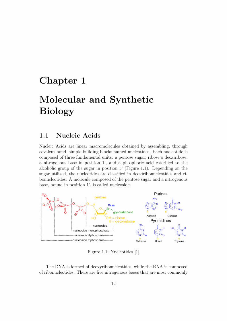

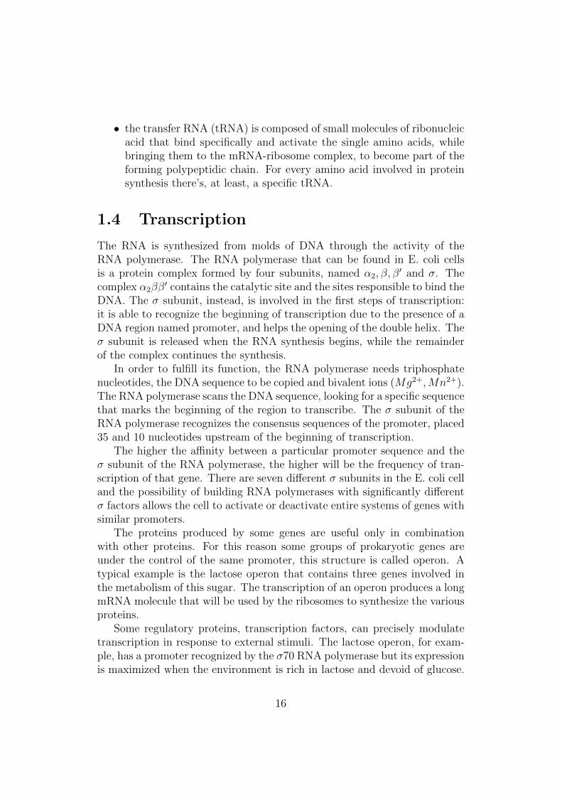
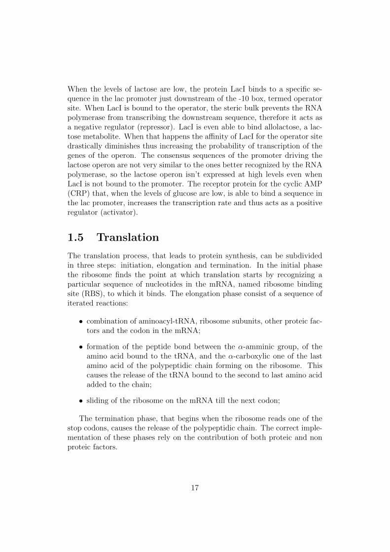
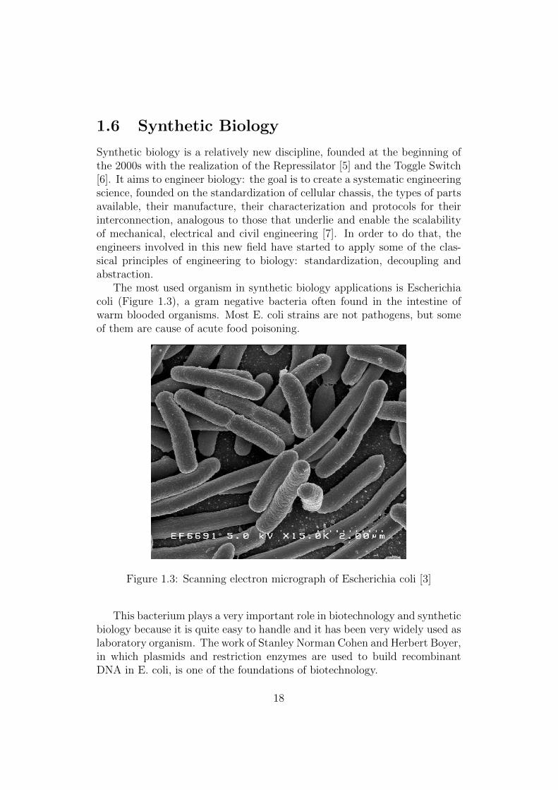
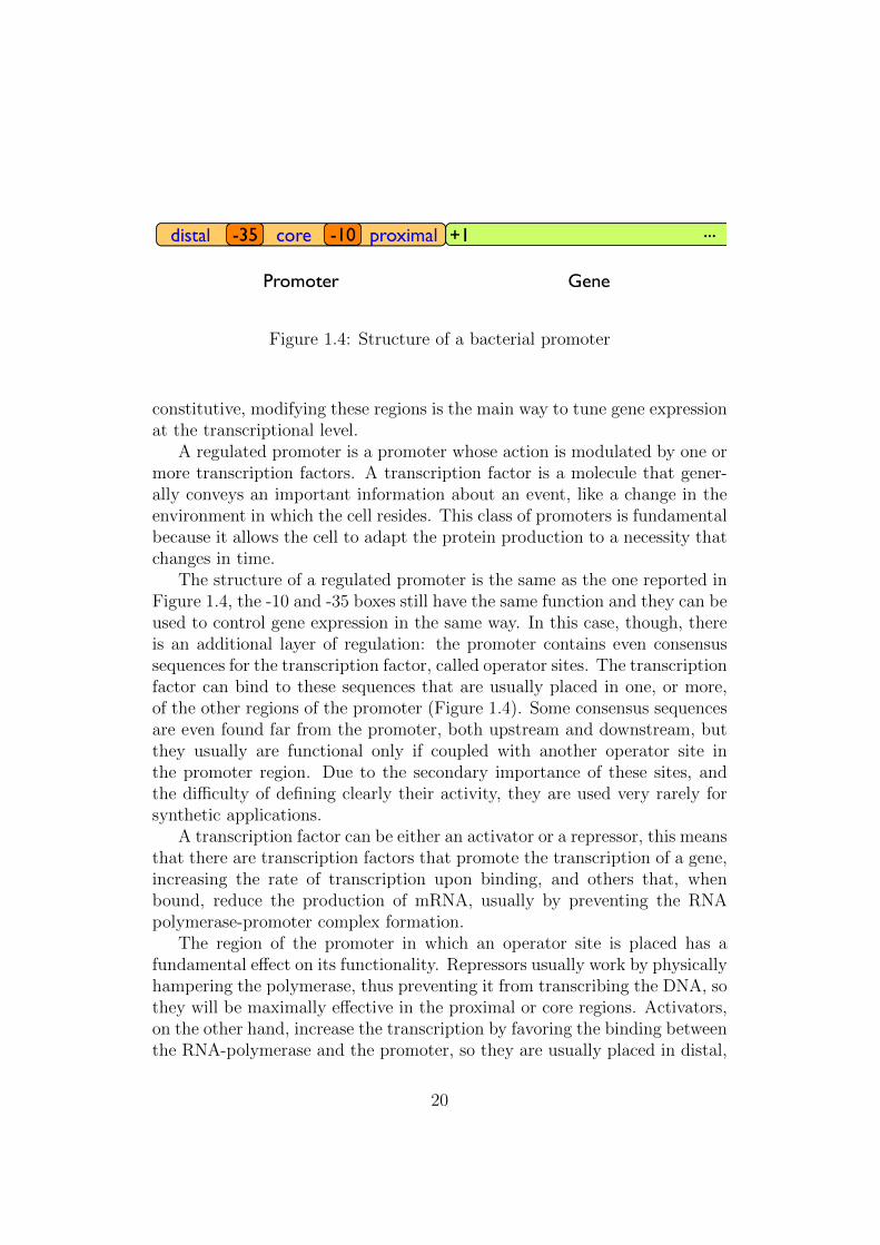
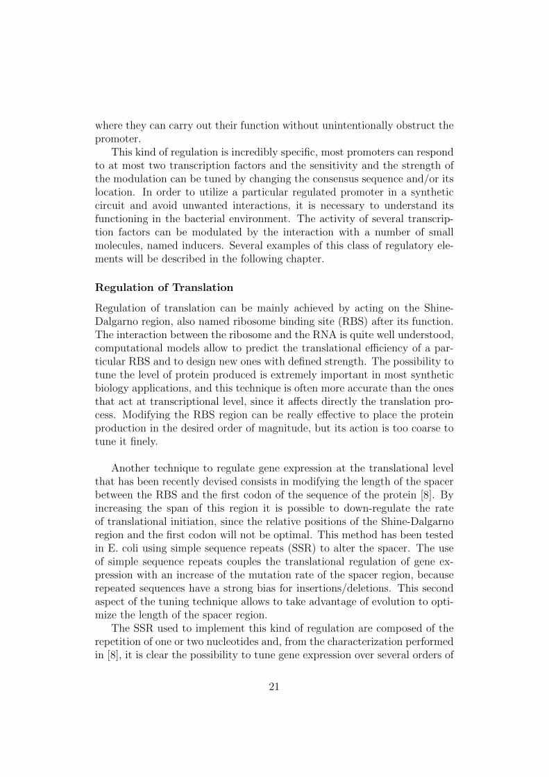
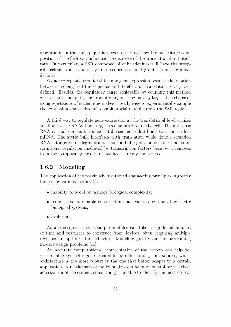
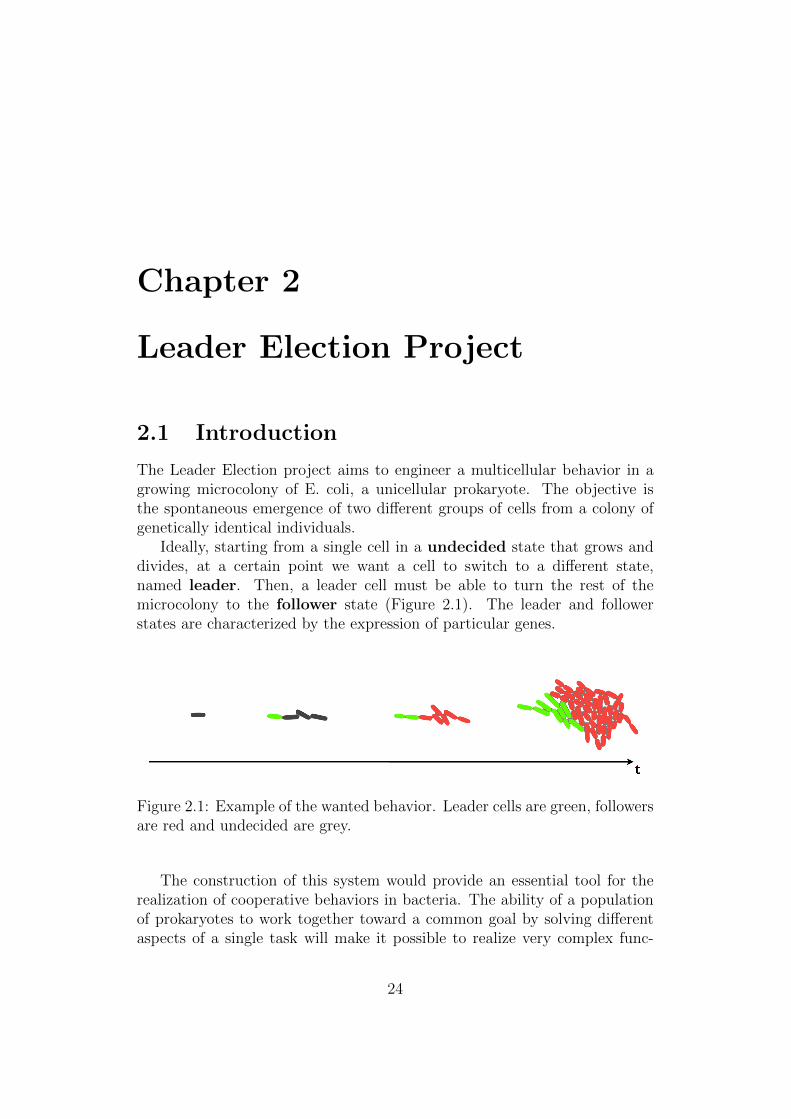


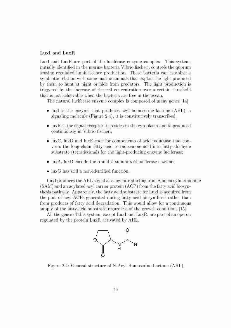
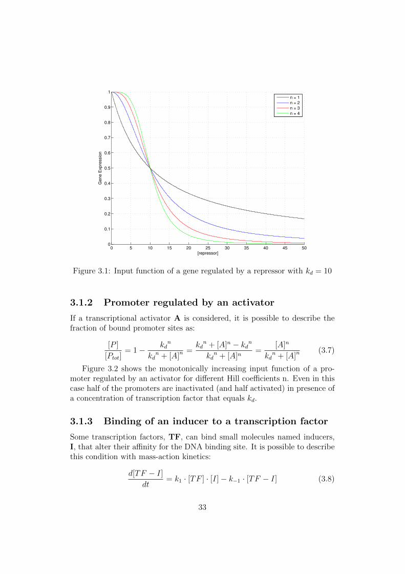
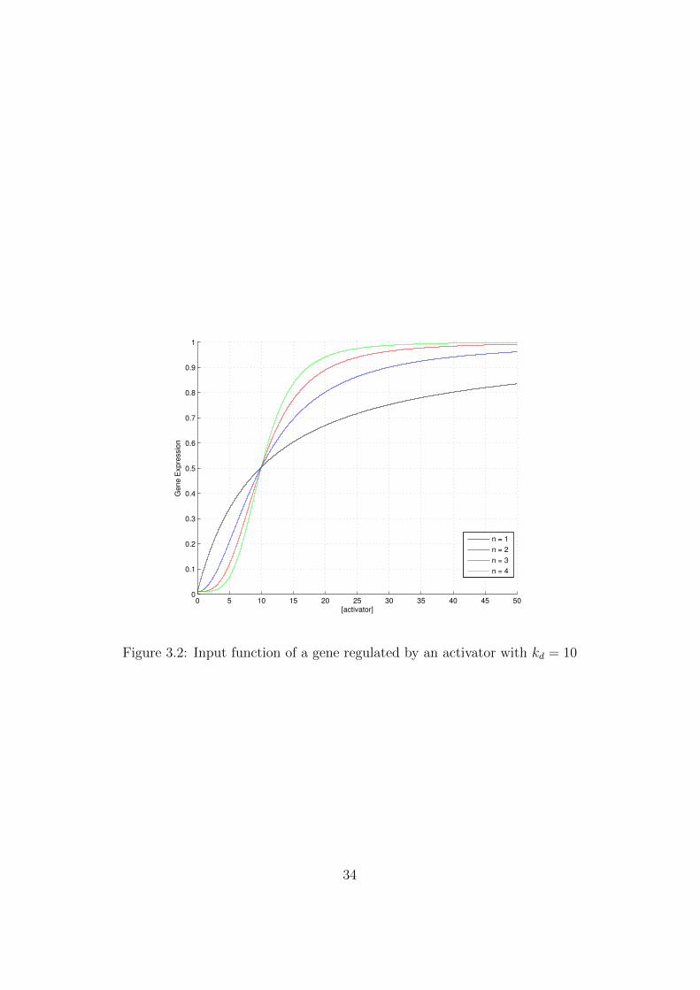

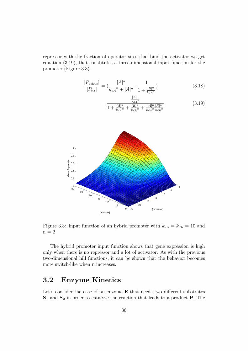
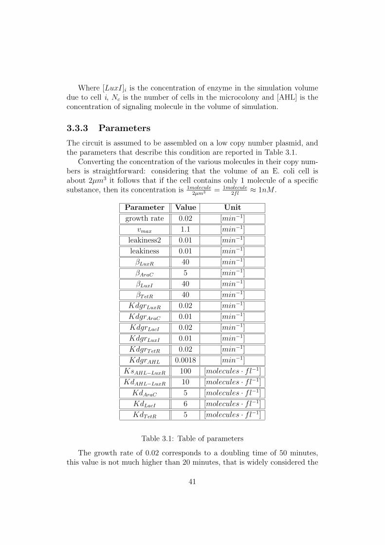

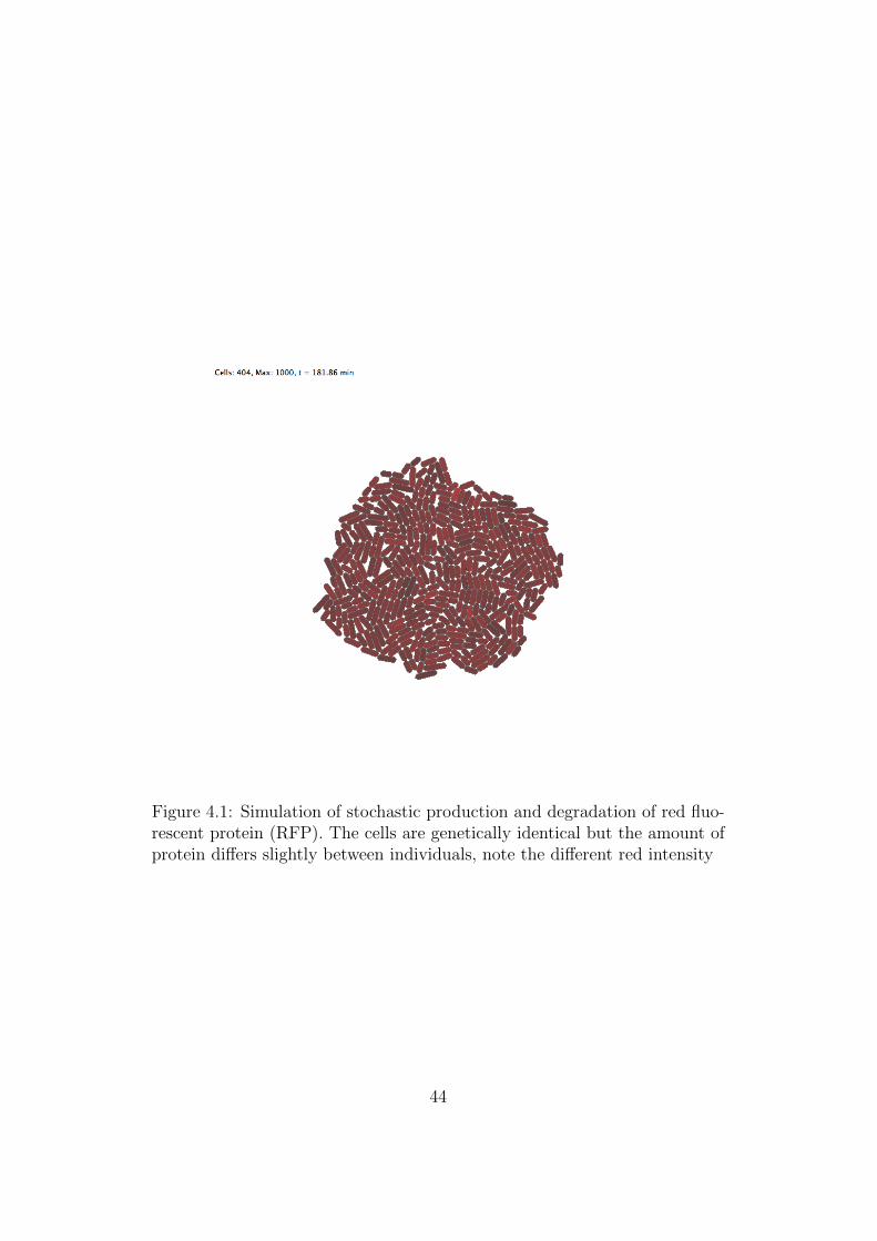
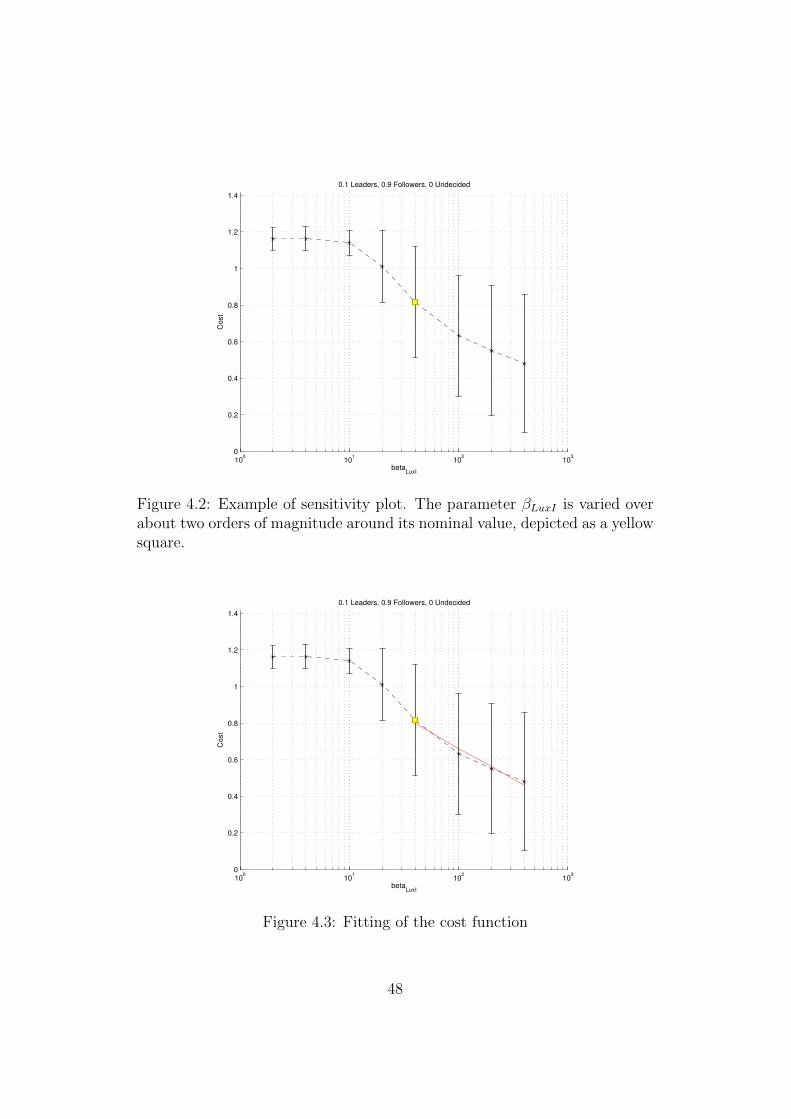
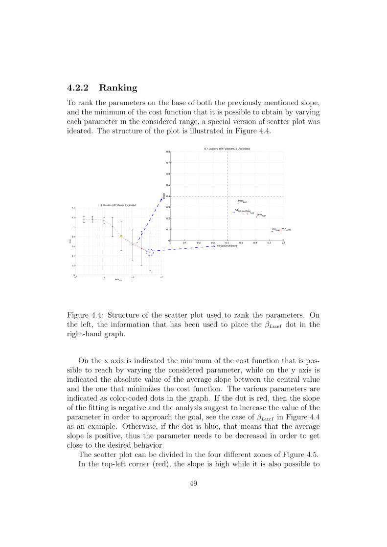
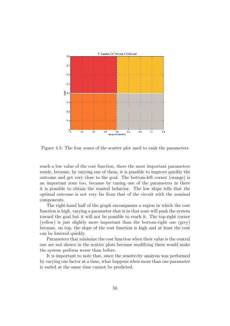
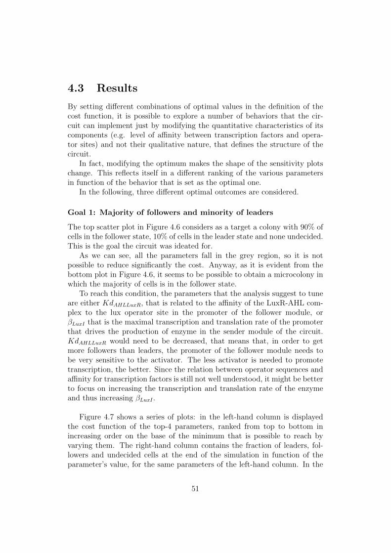
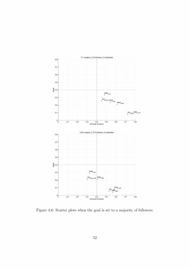

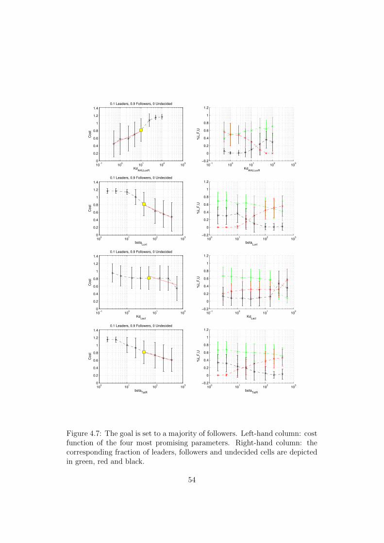
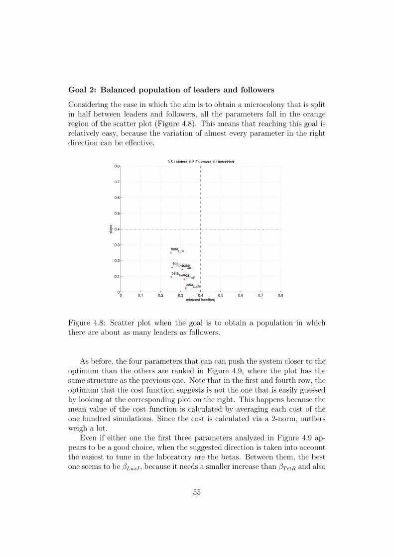
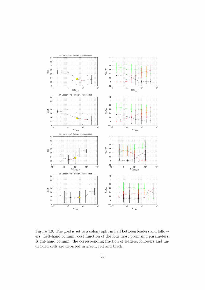
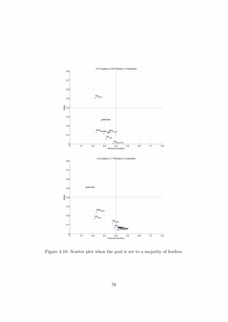
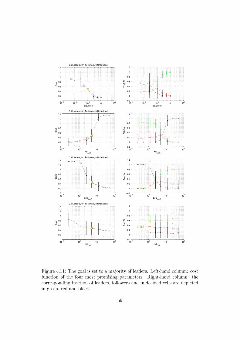
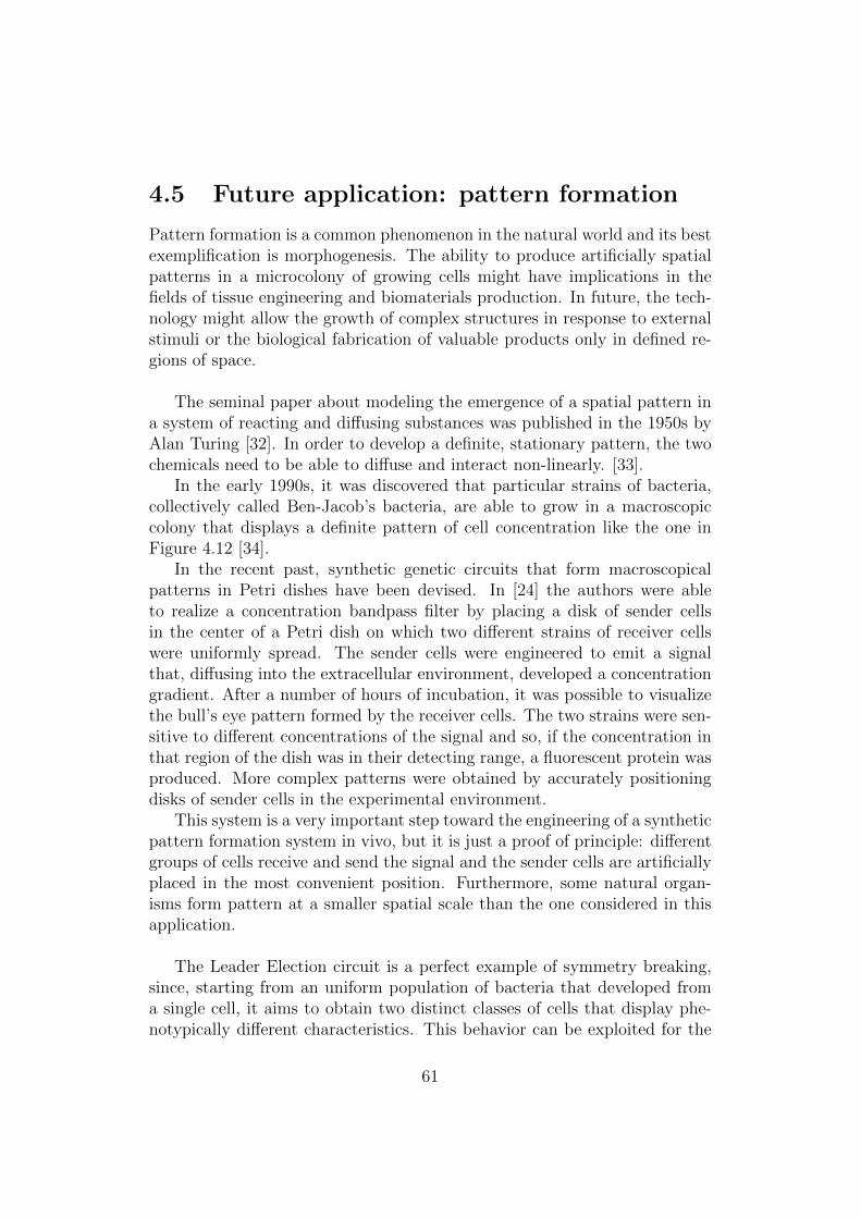
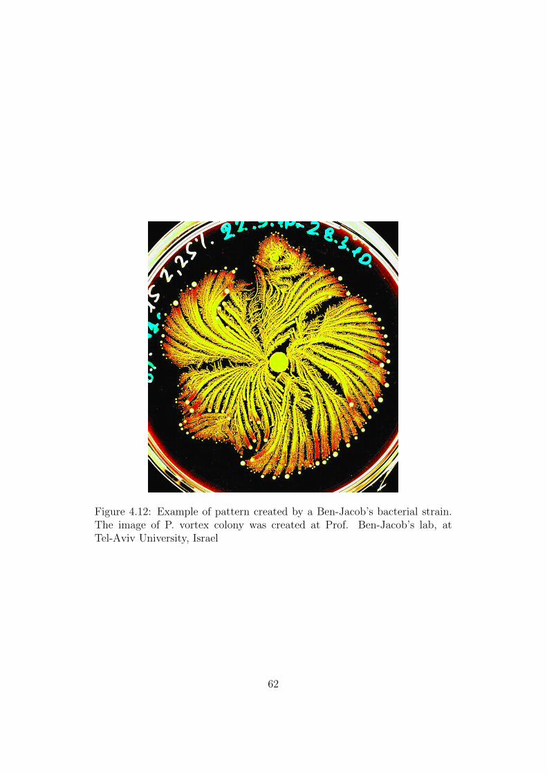

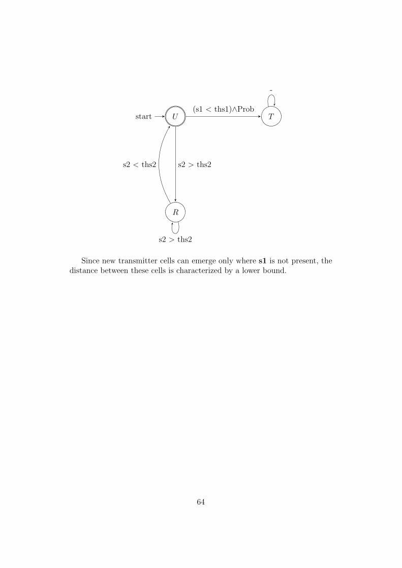
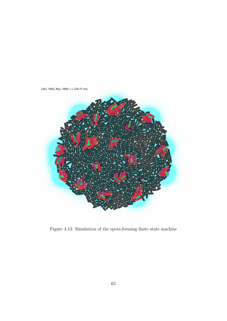
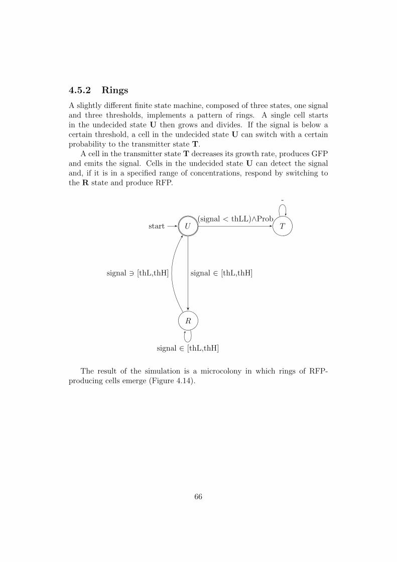
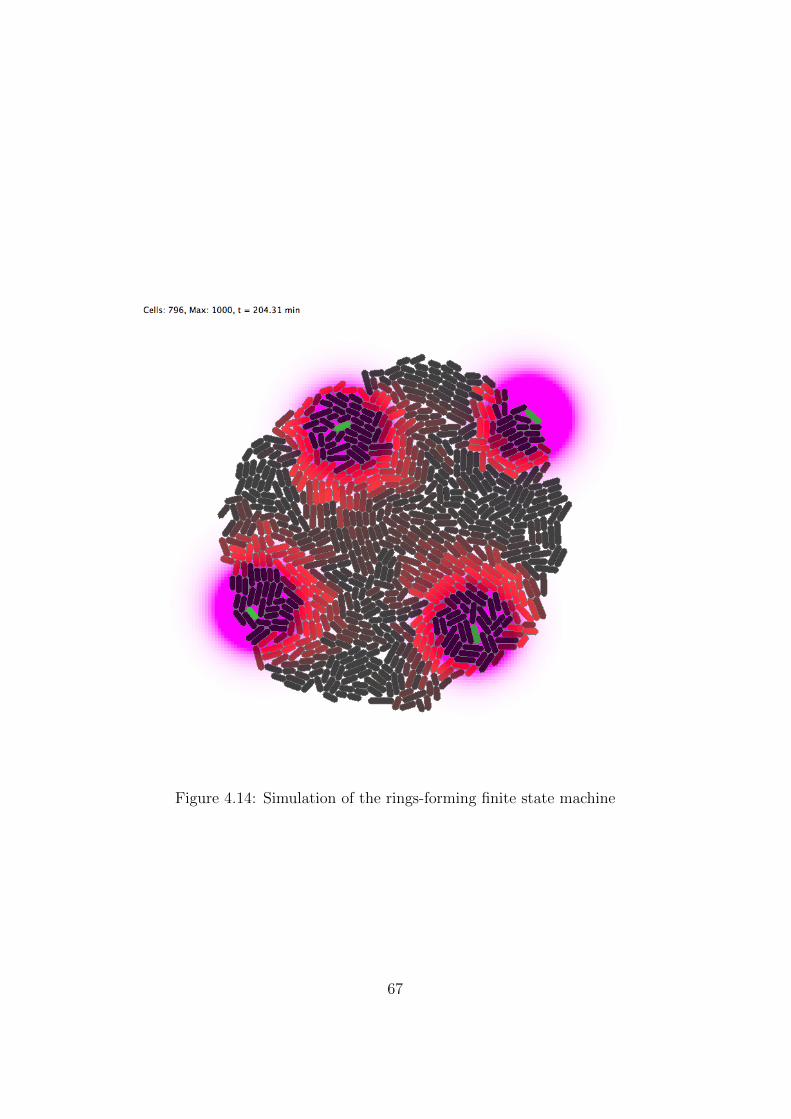
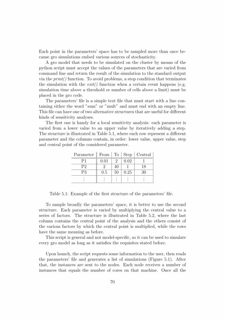
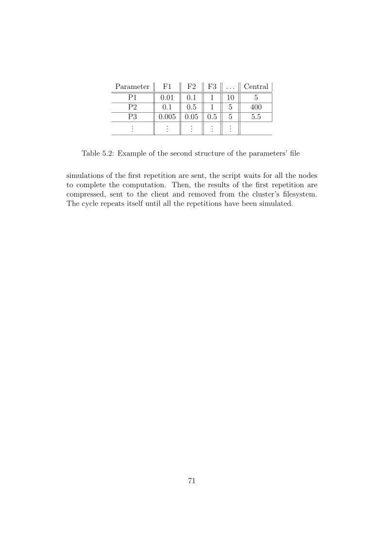
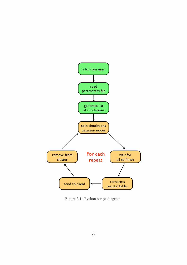
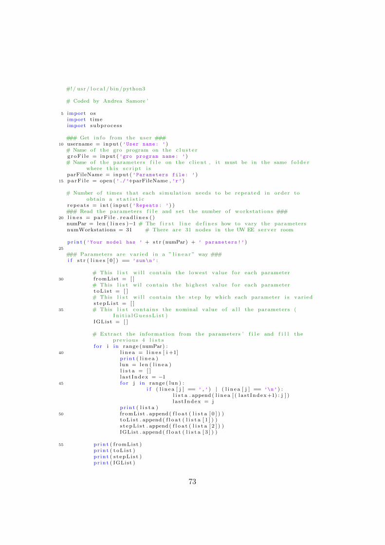

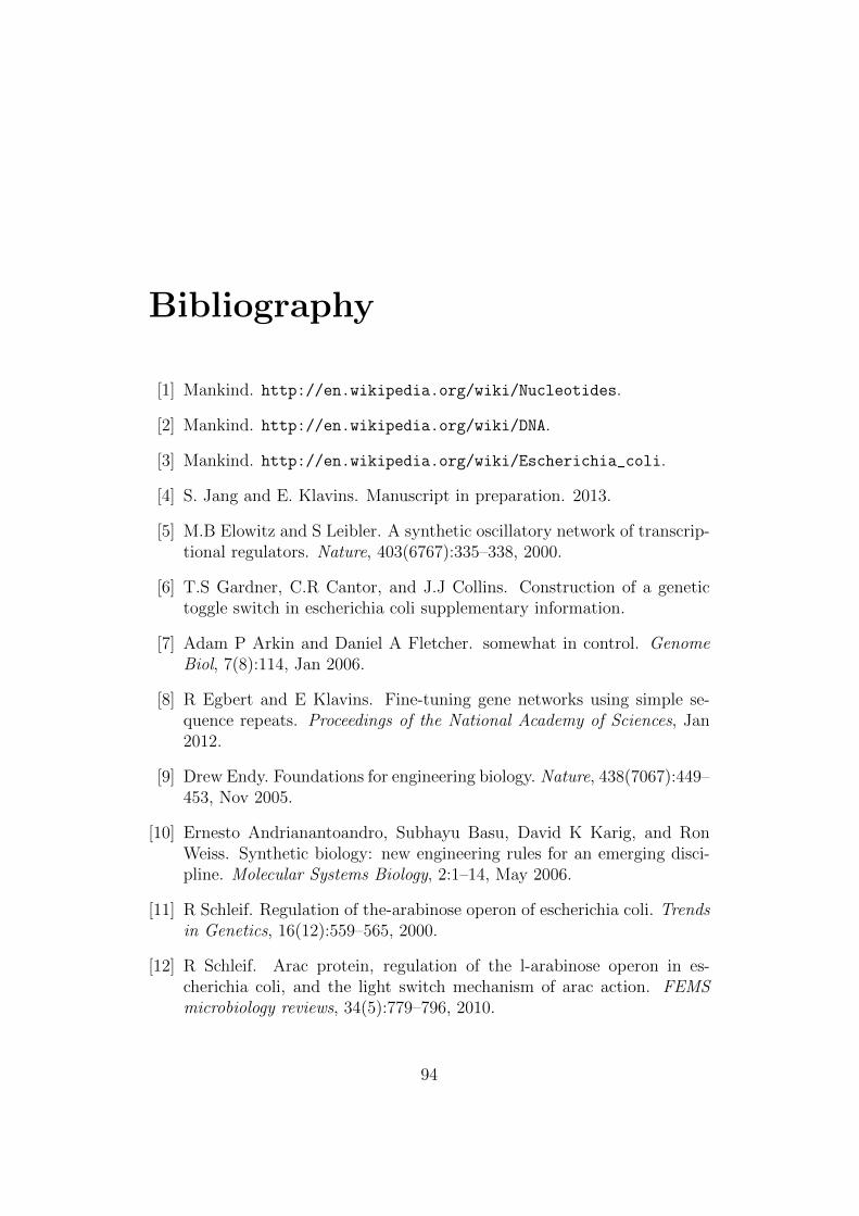


![ro STAT.] CONCURRENT RESOLUTIONS-JULY 7, 1966 … · ro STAT.] CONCURRENT RESOLUTIONS-JULY 7, 1966 B36 A-6334725, ... Jeanne also known as Chiu Kung-Chen. A-7863017, Klavins, Arvids](https://static.documents.pub/doc/80x56/5ae1fdeb7f8b9ae74a8bde3b/ro-stat-concurrent-resolutions-july-7-1966-stat-concurrent-resolutions-july.jpg)


